Design of an iterative auto-tuning algorithm for a fuzzy PID controller

This content has been downloaded from IOPscience. Please scroll down to see the full text.

Download details:

IP Address: 184.73.78.58

This content was downloaded on 20/10/2016 at 12:10

Please note that terms and conditions apply.

You may also be interested in:

Fuzzy control with amplitude/pulse-width modulation of nerve electrical stimulation for muscle

force control

C-C K Lin, W-C Liu, C-C Chan et al.

Force control of a tri-layer conducting polymer actuator using optimized fuzzy logic control

Mehmet Itik, Mohammadreza Sabetghadam and Gursel Alici

Firing rate control of a neuron using a linear PI controller

O Miranda-Domínguez, J Gonia and T I Netoff

Solar power plant performance evaluation: simulation and experimental validation

E M Natsheh and A Albarbar

Active control of flexible structures using a fuzzy logicalgorithm

Kelly Cohen, Tanchum Weller and Joseph

Z Ben-AsherFuzzy model reference learning control: a new control paradigm for smart structures

P Mayhan and G Washington

Artificial Intelligent Control for a Novel Advanced Microwave Biodiesel Reactor

W A Wali, K H Hassan, J D Cullen et al.

Design of an iterative auto-tuning algorithm for a fuzzy PID controller

View the table of contents for this issue, or go to the journal homepage for more

2012 J. Phys.: Conf. Ser. 364 012052

(http://iopscience.iop.org/1742-6596/364/1/012052)

Home Search Collections Journals About Contact us My IOPscience

http://iopscience.iop.org/page/terms

http://iopscience.iop.org/article/10.1088/1741-2560/9/2/026026








http://iopscience.iop.org/1742-6596/364/1

http://iopscience.iop.org/1742-6596

http://iopscience.iop.org/

http://iopscience.iop.org/search

http://iopscience.iop.org/collections

http://iopscience.iop.org/journals

http://iopscience.iop.org/page/aboutioppublishing

http://iopscience.iop.org/contact

http://iopscience.iop.org/myiopscience

Design of an iterative auto-tuning algorithm for a fuzzy PID

controller

Bakhtiar I Saeed and B Mehrdadi

School of Computing and Engineering,

University of Huddersfield

Queensgate, Huddersfield HD1 3DH, UK

[email protected], [email protected]

Abstract. Since the first application of fuzzy logic in the field of control engineering, it has

been extensively employed in controlling a wide range of applications. The human knowledge

on controlling complex and non-linear processes can be incorporated into a controller in the

form of linguistic terms. However, with the lack of analytical design study it is becoming more

difficult to auto-tune controller parameters. Fuzzy logic controller has several parameters that

can be adjusted, such as: membership functions, rule-base and scaling gains. Furthermore, it is

not always easy to find the relation between the type of membership functions or rule-base and

the controller performance. This study proposes a new systematic auto-tuning algorithm to fine

tune fuzzy logic controller gains. A fuzzy PID controller is proposed and applied to several

second order systems. The relationship between the closed-loop response and the controller

parameters is analysed to devise an auto-tuning method. The results show that the proposed

method is highly effective and produces zero overshoot with enhanced transient response. In

addition, the robustness of the controller is investigated in the case of parameter changes and

the results show a satisfactory performance.

1. Introduction

Since the first application of the fuzzy logic [1] in the field of control engineering field [2], an ever

increasing employment of fuzzy logic controllers have been reported [3, 4]. They have been

successfully applied in industrial processes and in some cases outperform conventional proportional-

integral-derivative (PID) controllers [5, 6], in particular when the controlled system is complex or non-

linear, as this is the case in many process control systems [7-9].

However the lack of a systematic method to design and tune these controllers may curtail their

applications [10-12]. In general, the design of fuzzy logic controller involves three stages [12-14].

Firstly, the rule-base is constructed by translating the experience of a skilled human operator on

controlling a plant into linguistic terms. Secondly, appropriate membership functions are selected. In

final stage, the scaling gains of the controller are determined. To achieve better performance the rule-

base, membership function parameters or the scaling gains are adjusted via trail-error-method or using

optimization tool techniques such as: Genetic Algorithms (GA) [15], Ant Colony Optimization

algorithm (ACO) [16], Shuffled Frog Leaping Algorithm (SFLA) [17] and Bees Algorithm (BA) [18].

The trial–and-error method is very simple and straightforward, but it is a tedious and a time-

consuming task [19], particularly when it is carried out on-line. Therefore, the technique is not always

practical. In the second method, although these tools are powerful and their successes have been

proved, they are computationally expensive [20]. Because they are population-based algorithms, a

25th International Congress on Condition Monitoring and Diagnostic Engineering IOP PublishingJournal of Physics: Conference Series 364 (2012) 012052 doi:10.1088/1742-6596/364/1/012052

Published under licence by IOP Publishing Ltd 1

mailto:[email protected]

mailto:[email protected]

considerable number of solutions are generated; individuals of these generations are needed to be

tested for their fitness functions. Additionally, some individuals cannot be tested in real-time and

safety-critical applications; therefore, they are best suited for simulation based designs, where the

plant transfer function is available.

Furthermore, there are other reasons that make the tuning process of fuzzy logic controllers more

complex. It is difficult to find the relation between selecting membership function type or rule base,

and the controller performance such as better rise time or less overshoot. In addition, unlike

conventional controllers, fuzzy logic controllers have several parameters that can be adjusted [21],

such as membership function shape, rules and scaling gains. Furthermore, there is no general rule of

tuning these parameters. However, some techniques applied in tuning conventional controllers can still

be utilised to some extent [12].

As in conventional PID controllers, there are various structures such as: fuzzy-proportional (FP),

fuzzy-proportional-derivative (FPD), fuzzy-proportional-integral (FPI) or fuzzy-incremental (FInc)

and fuzzy-proportional-integral-derivative (FPID) [13, 22-24]. Even for FPID controller, different

structures have been proposed. A normal FPID with three inputs (error, change in error and integral

error) has been proposed and implemented [24]. Although the controller has a simple structure, the

construction of a three-dimensional rule-base becomes more difficult as the number of rules increases

with the increasing number of inputs [13, 25]. Furthermore, constructing rules based on integral of

error is rather difficult [13].

To overcome these limitations parallel structure (FPI+FPD) [25] and FPD+I [13] have been

proposed. A Parallel structure which is a combination of FPI and FPD controllers has two inputs,

resulting in a two-dimensional rule-base. Additionally, it has the basic properties of a general PID

controller, but at the same time more computational time is required to compute the controller output

as there are two fuzzy logic controllers in the structure. The FPD+I is constructed by combining a

crisp integral action with FPD controller, hence the rule-base is two-dimensional and the controller has

the merits of a general PID controller. Further configurations have been found in the literature such as:

FPID with incremental output [26], rule coupled FPI+FPD [26], rule de-coupled FPID [26], FP+I+D

[23], and FPI+D [23] controllers.

In this paper, an auto-tuning algorithm is designed to tune a fuzzy PID controller. The controller is

applied to different second order systems. Initially, the controller gains are fixed and then

automatically tuned to achieve the best possible performance. The results show that the proposed

method is highly effective and produces zero overshoot with enhanced transient response. In addition,

the robustness of the controller is investigated in the case of system parameter changes and the results

show a satisfactory performance.

The remainder of this paper is organised as follows: section 2 presents an overview of the fuzzy

logic controller structure and the fuzzy PID simulation design model. The auto-tuning algorithm is

illustrated in section 3. Evaluation and simulation results are shown in section 4. Finally, some

conclusions are drawn in section 5.

2. Controller design structure

In this section, detailed structure of the fuzzy logic controller and the simulation model are given.

2.1. Fuzzy PD+I controller structure

The Fuzzy PD+I controller reported in [13] is shown in figure 1. It was adopted as the controller in

this paper; therefore its structure is illustrated in some details.


2

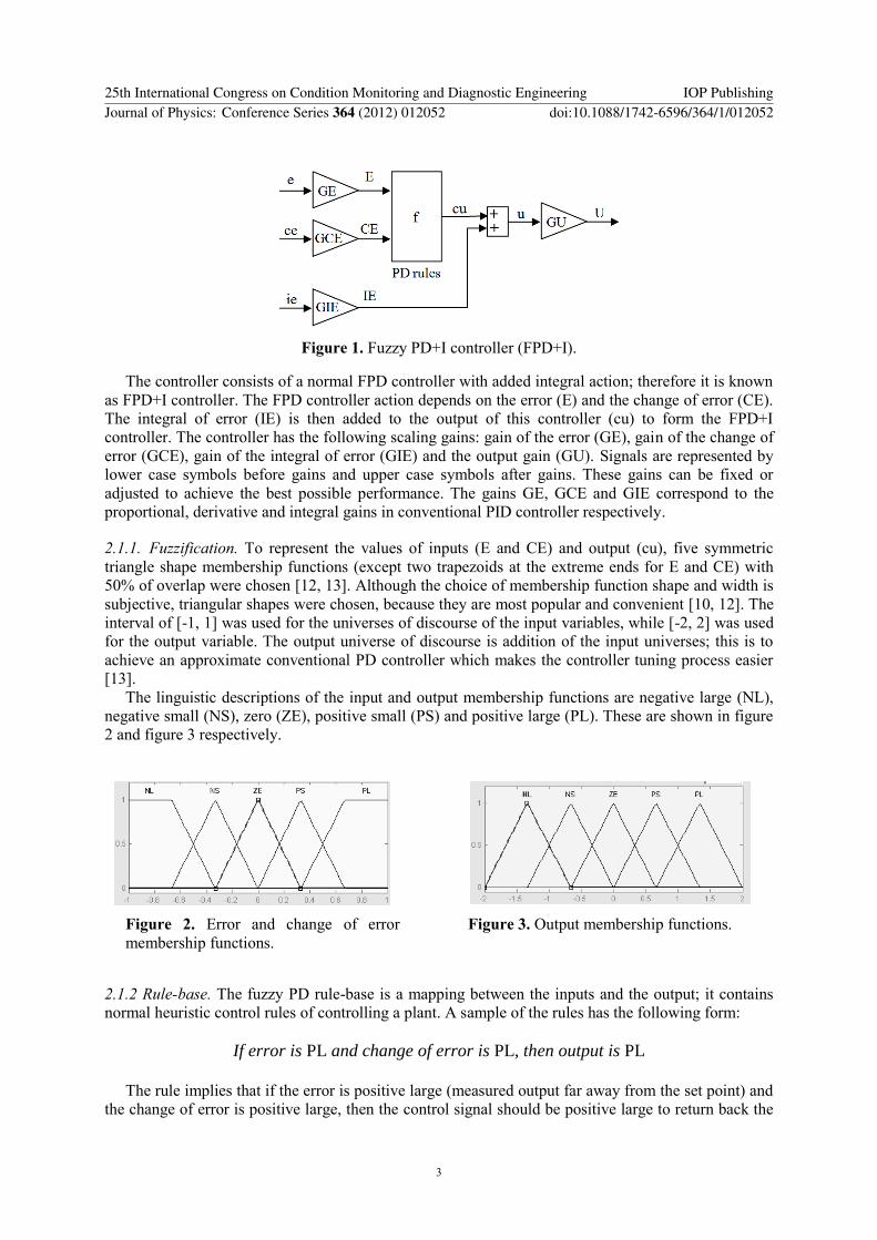
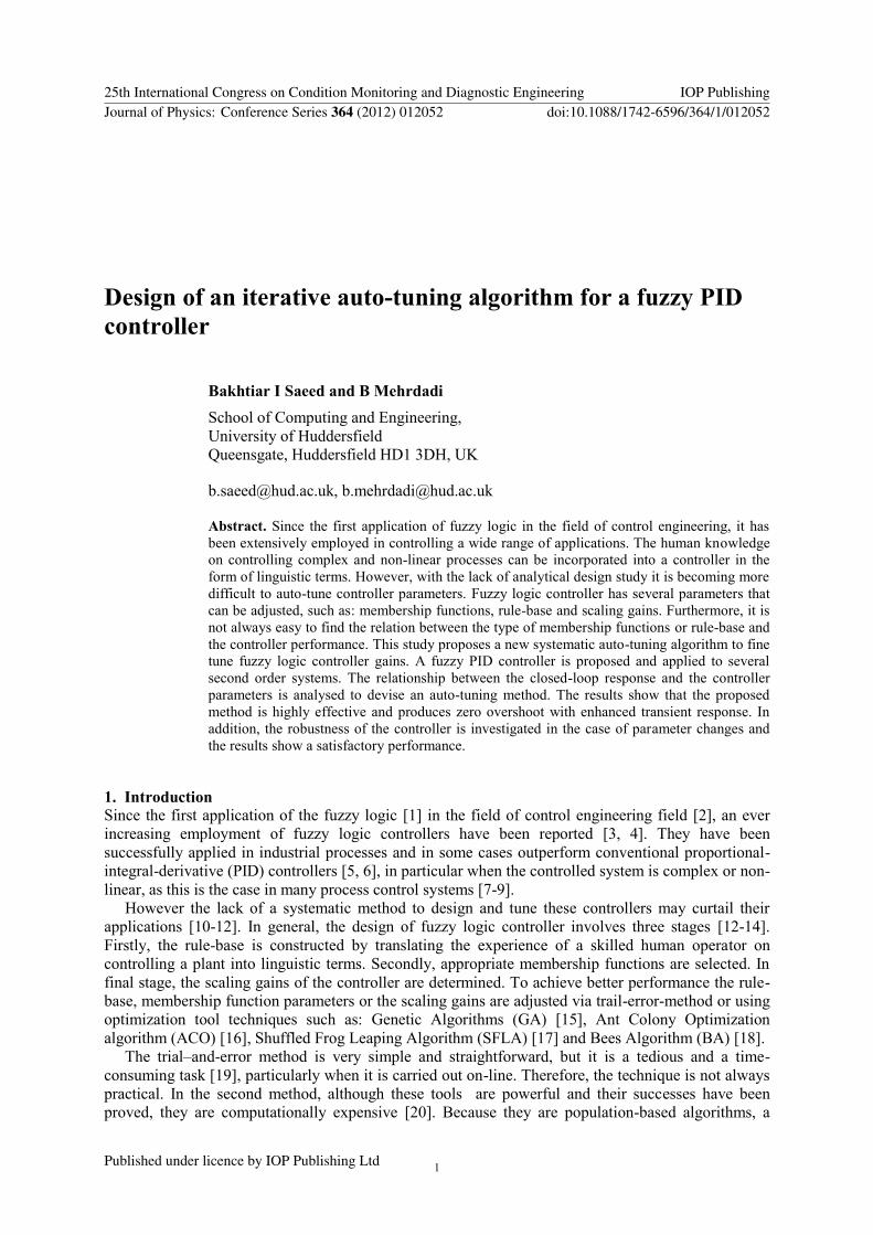
Figure 1. Fuzzy PD+I controller (FPD+I).

The controller consists of a normal FPD controller with added integral action; therefore it is known

as FPD+I controller. The FPD controller action depends on the error (E) and the change of error (CE).

The integral of error (IE) is then added to the output of this controller (cu) to form the FPD+I

controller. The controller has the following scaling gains: gain of the error (GE), gain of the change of

error (GCE), gain of the integral of error (GIE) and the output gain (GU). Signals are represented by

lower case symbols before gains and upper case symbols after gains. These gains can be fixed or

adjusted to achieve the best possible performance. The gains GE, GCE and GIE correspond to the

proportional, derivative and integral gains in conventional PID controller respectively.

2.1.1. Fuzzification. To represent the values of inputs (E and CE) and output (cu), five symmetric

triangle shape membership functions (except two trapezoids at the extreme ends for E and CE) with

50% of overlap were chosen [12, 13]. Although the choice of membership function shape and width is

subjective, triangular shapes were chosen, because they are most popular and convenient [10, 12]. The

interval of [-1, 1] was used for the universes of discourse of the input variables, while [-2, 2] was used

for the output variable. The output universe of discourse is addition of the input universes; this is to

achieve an approximate conventional PD controller which makes the controller tuning process easier

[13].

The linguistic descriptions of the input and output membership functions are negative large (NL),

negative small (NS), zero (ZE), positive small (PS) and positive large (PL). These are shown in figure

2 and figure 3 respectively.

Figure 2. Error and change of error

membership functions.

Figure 3. Output membership functions.

2.1.2 Rule-base. The fuzzy PD rule-base is a mapping between the inputs and the output; it contains

normal heuristic control rules of controlling a plant. A sample of the rules has the following form:

If error is PL and change of error is PL, then output is PL

The rule implies that if the error is positive large (measured output far away from the set point) and

the change of error is positive large, then the control signal should be positive large to return back the


3

output near the setpoint. As there are 5 linguistic variables for each input, 25 rules were created, table

1 shows the rules.

Table 1. Fuzzy PD+I controller (FPD+I).

Controller

Output (cu)

Change of error (CE)

NL NS ZE PS PL

Error

(E)

NL NL NL NS NS ZE

NS NL NS NS ZE PS

ZE NS NS ZE PS PS

PS NS ZE PS PS PL

PL ZE PS PS PL PL

2.1.3 Defuzzification. The minimum (Min) operator was selected as an implication method, and the

most popular and standard method of defuzzification process known as centre of gravity (CoG) was

selected.

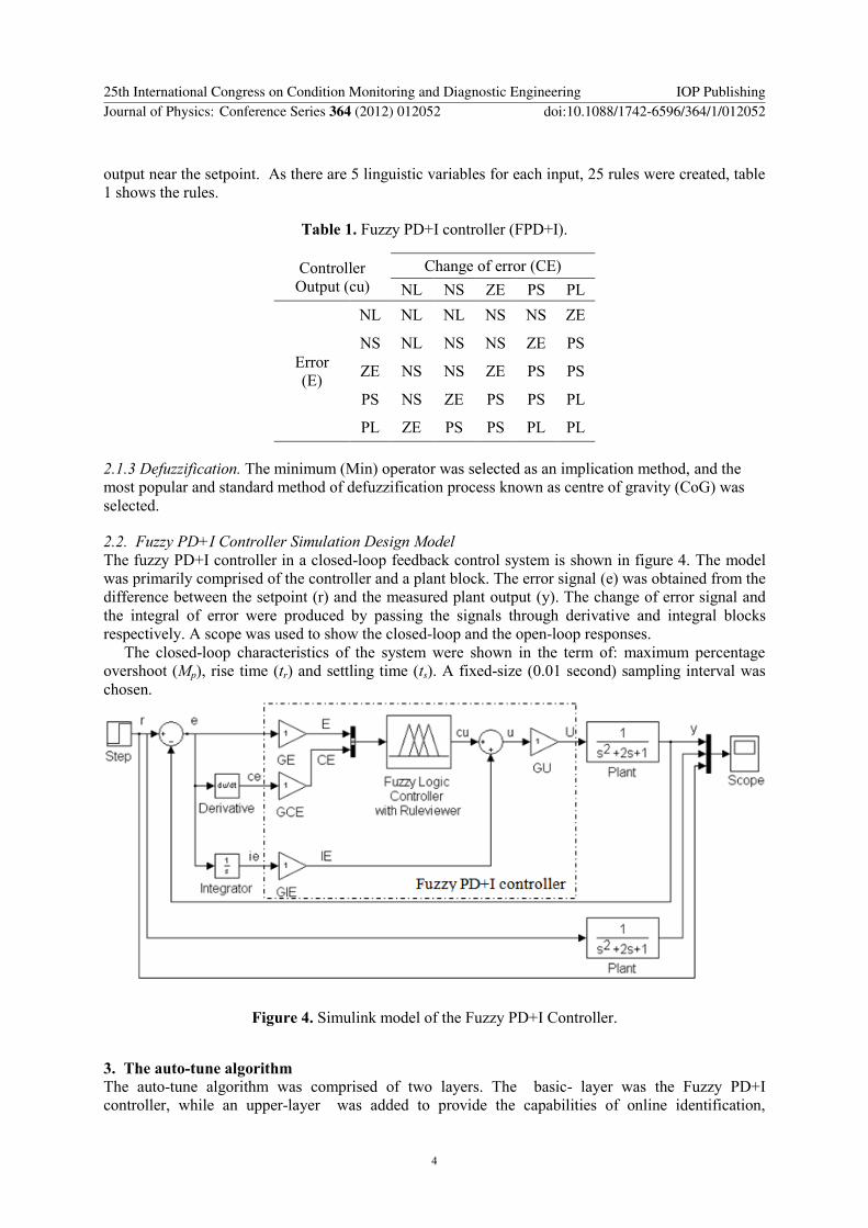
2.2. Fuzzy PD+I Controller Simulation Design Model

The fuzzy PD+I controller in a closed-loop feedback control system is shown in figure 4. The model

was primarily comprised of the controller and a plant block. The error signal (e) was obtained from the

difference between the setpoint (r) and the measured plant output (y). The change of error signal and

the integral of error were produced by passing the signals through derivative and integral blocks

respectively. A scope was used to show the closed-loop and the open-loop responses.

The closed-loop characteristics of the system were shown in the term of: maximum percentage

overshoot (Mp), rise time (tr) and settling time (ts). A fixed-size (0.01 second) sampling interval was

chosen.

Figure 4. Simulink model of the Fuzzy PD+I Controller.

3. The auto-tune algorithm

The auto-tune algorithm was comprised of two layers. The basic- layer was the Fuzzy PD+I

controller, while an upper-layer was added to provide the capabilities of online identification,


4

adaptation and auto-tuning to the basic-layer controller by determining appropriate values of the

controller gains based on the evaluation of the system performance. Additionally, it has the ability to

monitor the performance of the system and to guarantee the stability.

The details of the algorithm can be summarised as follows. First, a closed-loop test on the system is

performed by applying the fuzzy PD+I controller. The controller gains are set to their default values

(one). The output is bounded and the overshoot is not allowed to exceed 100%, where the system

becomes unstable. Secondly, if the response exhibits an overshoot with amplitude higher than 1%, the

overshoot is measured and the values of GU and GIE are calculated as follows:

GU = Mp (1)

GIE = 1 / (2 * Mp) (2)

Where Mp is the maximum percentage overshoot. This significantly reduces the overshoot. The

gains are kept unchanged when the overshoot is less than 1%. Then, to improve the rise-time, the

value of GCE is decreased. Finally, if the system performance is not satisfactory the value of GIE is

increased. The last two steps are performed in an iterative base and the integrated square error (ISE)

and the maximum percentage overshoot (Mp) were chosen to measure the performance of the

controller.

The black diagram and the flowchart of the auto-tune algorithm are shown in figure 5 and figure 6

respectively.

Figure 5. The block diagram of the auto-tune algorithm.


5

Figure 6. The flowchart of the auto-tune algorithm.

4. Evaluation of the auto-tuning algorithm

4.1. Transfer Function Model

In order to evaluate the algorithm and to cover a wide range of systems, several standard second order

systems with different characteristics were simulated.

Many real-time applications exhibit oscillation and overshoot in their step responses, these

characteristics can be modelled using a second order system [27, 28]. Furthermore, this will help

understand the response of higher order systems. Consider the standard second order transfer function

[29, 30] in equation (3).

(3)

Yes

No

Yes

Yes

No

No

A closed-loop test is performed by applying the Fuzzy PD+I controller with fixed gains.

Start

Is Mp > 1%

Is tr

satisfactory? Decrease GCE

Is system

performance

satisfactory?

End

Measure the overshoot (Mp) and set the gains

as follows: GU = Mp, GIE = 1 / (2 * Mp)

Increase GIE


6

Where is the gain, (zeta) is the damping ratio and n is the natural frequency. The system has

different responses depending on the location of poles. The poles of equation (3) are the roots of the

denominator and can be determined as:

p1, p2-n ± √ ²n (4)

The value of determines whether the poles are real or complex conjugate. From equation (3)

suppose = 1 and n = 1, depending on the value of there are five distinct cases as following:

If ≥ 1, the poles are real:

= 1, critically damped system, denoted as case 1.

>1, overdamped system, denoted as case 2.

If 0 ≤ 1, the poles are complex conjugate:

= 0, undamped (marginally stable), denoted as case 4.

=0.5, underdamped system, denoted as case 3.

If 0, unstable system, denoted as case 5.

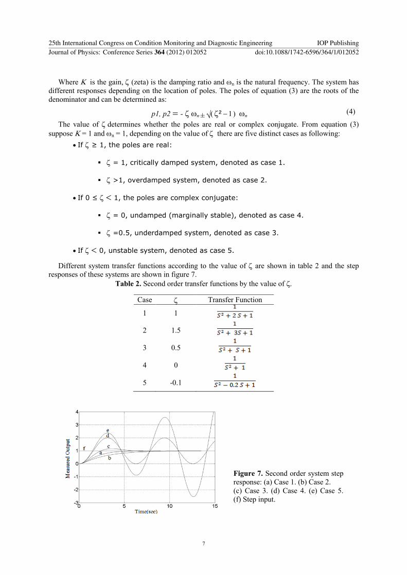
Different system transfer functions according to the value of are shown in table 2 and the step

responses of these systems are shown in figure 7.

Table 2. Second order transfer functions by the value of

Case Transfer Function

1 1

2 1.5

3 0.5

4 0

5 -0.1

Figure 7. Second order system step

response: (a) Case 1. (b) Case 2.

(c) Case 3. (d) Case 4. (e) Case 5.

(f) Step input.


7

4.2. Auto-tune algorithm results

The controller with the auto-tune algorithm was applied to all the second order cases mentioned in the

previous section. Due to the limited space of the paper only the step responses of the case 3 and case 5

which represent underdamped and unstable systems are shown in figure 8 - figure 13. The auto-tuned

gains, open-loop and close-loop performance measures are shown in table 3.

Figure 8. Step response of case 3, iteration 1 - iteration 5.




8





9

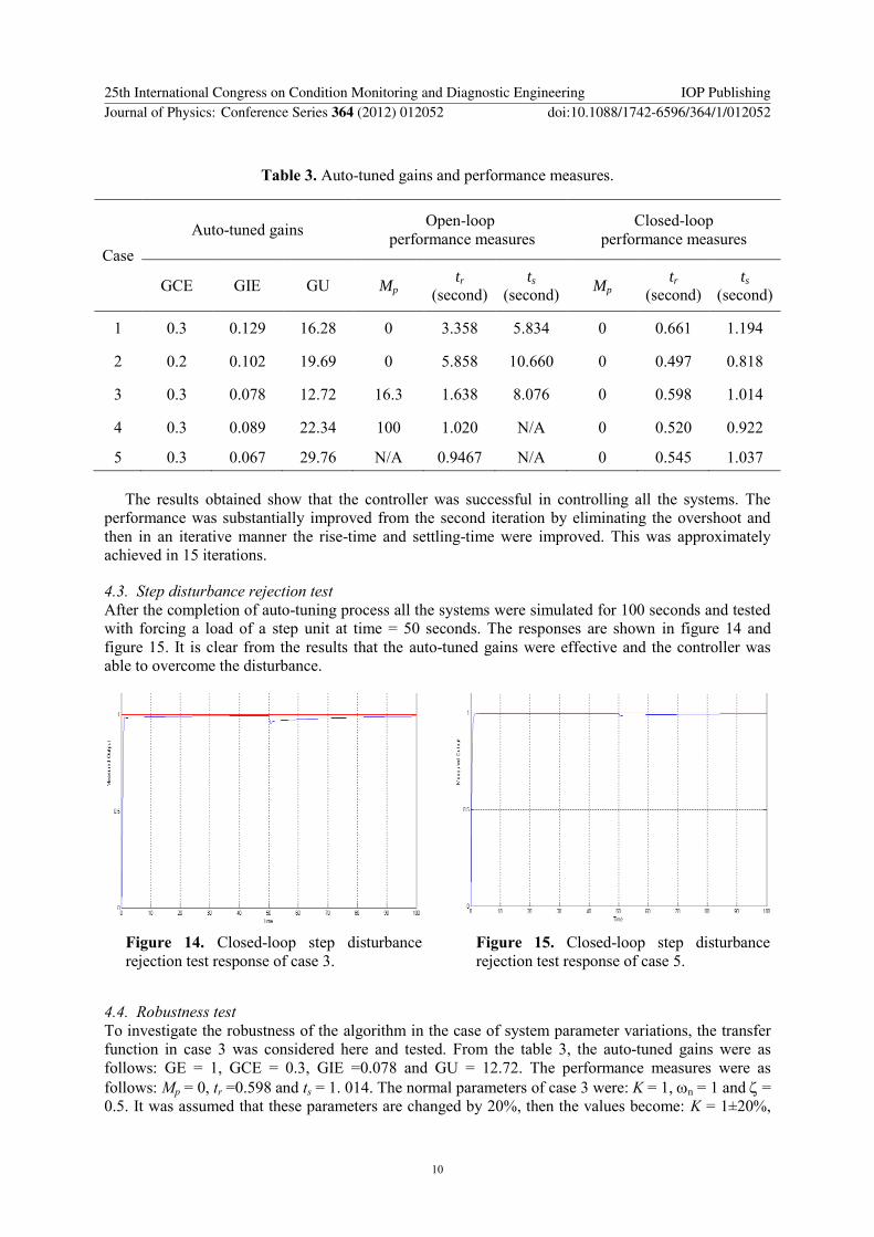
Table 3. Auto-tuned gains and performance measures.

Case

Auto-tuned gains Open-loop

performance measures

Closed-loop

performance measures

GCE GIE GU Mp

tr

(second)

ts

(second) Mp

tr

(second)

ts

(second)

1 0.3 0.129 16.28 0 3.358 5.834 0 0.661 1.194

2 0.2 0.102 19.69 0 5.858 10.660 0 0.497 0.818

3 0.3 0.078 12.72 16.3 1.638 8.076 0 0.598 1.014

4 0.3 0.089 22.34 100 1.020 N/A 0 0.520 0.922

5 0.3 0.067 29.76 N/A 0.9467 N/A 0 0.545 1.037

The results obtained show that the controller was successful in controlling all the systems. The

performance was substantially improved from the second iteration by eliminating the overshoot and

then in an iterative manner the rise-time and settling-time were improved. This was approximately

achieved in 15 iterations.

4.3. Step disturbance rejection test

After the completion of auto-tuning process all the systems were simulated for 100 seconds and tested

with forcing a load of a step unit at time = 50 seconds. The responses are shown in figure 14 and

figure 15. It is clear from the results that the auto-tuned gains were effective and the controller was

able to overcome the disturbance.

Figure 14. Closed-loop step disturbance

rejection test response of case 3.

Figure 15. Closed-loop step disturbance

rejection test response of case 5.

4.4. Robustness test

To investigate the robustness of the algorithm in the case of system parameter variations, the transfer

function in case 3 was considered here and tested. From the table 3, the auto-tuned gains were as

follows: GE = 1, GCE = 0.3, GIE =0.078 and GU = 12.72. The performance measures were as

follows: Mp = 0, tr =0.598 and ts = 1. 014. The normal parameters of case 3 were: K = 1, n = 1 and =

0.5. It was assumed that these parameters are changed by 20%, then the values become: K = 1±20%,


10

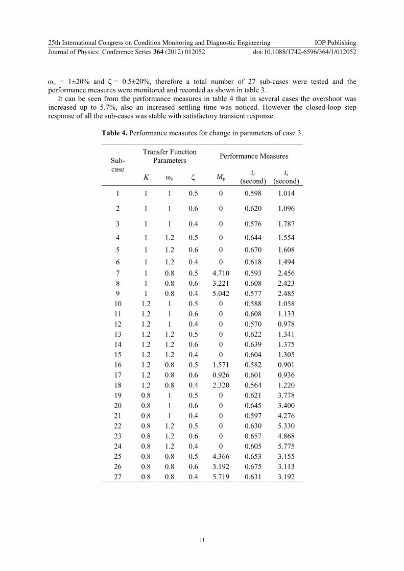
n = 1±20% and = 0.5±20%, therefore a total number of 27 sub-cases were tested and the

performance measures were monitored and recorded as shown in table 3.

It can be seen from the performance measures in table 4 that in several cases the overshoot was

increased up to 5.7%, also an increased settling time was noticed. However the closed-loop step

response of all the sub-cases was stable with satisfactory transient response.

Table 4. Performance measures for change in parameters of case 3.

Sub-

case

Transfer Function

Parameters Performance Measures

n Mp

tr

(second)

ts

(second)

1 1 1 0.5 0 0.598 1.014

2 1 1 0.6 0 0.620 1.096

3 1 1 0.4 0 0.576 1.787

4 1 1.2 0.5 0 0.644 1.554

5 1 1.2 0.6 0 0.670 1.608

6 1 1.2 0.4 0 0.618 1.494

7 1 0.8 0.5 4.710 0.593 2.456

8 1 0.8 0.6 3.221 0.608 2.423

9 1 0.8 0.4 5.042 0.577 2.485

10 1.2 1 0.5 0 0.588 1.058

11 1.2 1 0.6 0 0.608 1.133

12 1.2 1 0.4 0 0.570 0.978

13 1.2 1.2 0.5 0 0.622 1.341

14 1.2 1.2 0.6 0 0.639 1.375

15 1.2 1.2 0.4 0 0.604 1.305

16 1.2 0.8 0.5 1.571 0.582 0.901

17 1.2 0.8 0.6 0.926 0.601 0.936

18 1.2 0.8 0.4 2.320 0.564 1.220

19 0.8 1 0.5 0 0.621 3.778

20 0.8 1 0.6 0 0.645 3.400

21 0.8 1 0.4 0 0.597 4.276

22 0.8 1.2 0.5 0 0.630 5.330

23 0.8 1.2 0.6 0 0.657 4.868

24 0.8 1.2 0.4 0 0.605 5.775

25 0.8 0.8 0.5 4.366 0.653 3.155

26 0.8 0.8 0.6 3.192 0.675 3.113

27 0.8 0.8 0.4 5.719 0.631 3.192


11

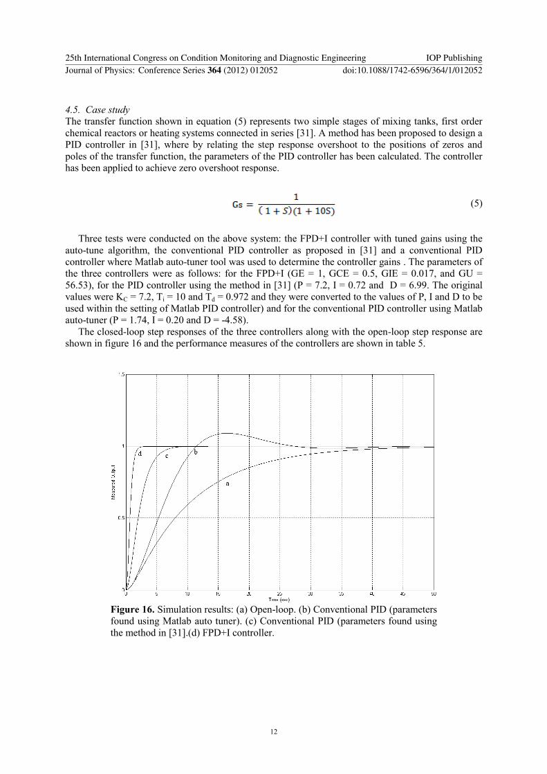
4.5. Case study

The transfer function shown in equation (5) represents two simple stages of mixing tanks, first order

chemical reactors or heating systems connected in series [31]. A method has been proposed to design a

PID controller in [31], where by relating the step response overshoot to the positions of zeros and

poles of the transfer function, the parameters of the PID controller has been calculated. The controller

has been applied to achieve zero overshoot response.

(5)

Three tests were conducted on the above system: the FPD+I controller with tuned gains using the

auto-tune algorithm, the conventional PID controller as proposed in [31] and a conventional PID

controller where Matlab auto-tuner tool was used to determine the controller gains . The parameters of

the three controllers were as follows: for the FPD+I (GE = 1, GCE = 0.5, GIE = 0.017, and GU =

56.53), for the PID controller using the method in [31] (P = 7.2, I = 0.72 and D = 6.99. The original

values were KC = 7.2, Ti = 10 and Td = 0.972 and they were converted to the values of P, I and D to be

used within the setting of Matlab PID controller) and for the conventional PID controller using Matlab

auto-tuner (P = 1.74, I = 0.20 and D = -4.58).

The closed-loop step responses of the three controllers along with the open-loop step response are

shown in figure 16 and the performance measures of the controllers are shown in table 5.

Figure 16. Simulation results: (a) Open-loop. (b) Conventional PID (parameters

found using Matlab auto tuner). (c) Conventional PID (parameters found using

the method in [31].(d) FPD+I controller.


12

Table 5. The performance measures of each controller.

Close-loop step response

Performance

Measures Open-loop

Conventional PID

(parameters found

using Matlab auto-

tuner)

Conventional PID

(parameters found

using the method in

[31])

Fuzzy FPD+I

(parameters found

using the auto-tune

algorithm)

Mp 0 8.9 0 0

tr (second) 22.15 7.855 3.96 1.086

ts (second) 40.17 24.530 6.9 1.908

It is evident from the results that the auto-tune algorithm was highly effective and response of the

FPD+I controller has achieved zero overshoot with faster rise time and shorter settling time compared

to other PID controllers.

5. Conclusions

An auto-tune algorithm for a fuzzy PID controller has been designed and applied to several second

order systems. The results have been encouraging and indicate the validity of the technique where the

performance of the system response progressively improves as the system is subjected to new step

inputs. The results also showed that the algorithm was highly effective in achieving zero overshoot

and produced a faster transient response. In addition, the robustness of the algorithm was investigated

in the case of system parameter changes and the results showed a satisfactory performance.

A case study result showed that the auto-tuning algorithm outperformed the conventional PID

controller in terms of achieving zero overshoot and faster transient response.

References

[1] Zadeh L 1965 Fuzzy sets Information and Control 8 338-53

[2] Mamdani E and Assilian S 1975 An experiment in linguistic synthesis with a fuzzy logic

controller Int. J. of Man-Machine Studies 7 1-13

[3] Kumar V and B Naapm 2011 A review on classical and fuzzy pid controllers Int. J. of

Intelligent control and sys. 16-3 170-81

[4] Shen Q 2088 Special issue on UK fuzzy systems research Int. J. of Computational Intelligence

Res. 4 297–9

[5] Vaishnav S and Khan Z 2007 Design and performance of pid and fuzzy logic controller with

smaller rule set for higher order system Proc. of the World Congress on Engineering and

Computer Sci. (San Francisco, USA) (Citeseer) p 24-6

[6] Saeed B and Mehrdadi B 2011 Zero overshoot and fast transient response using a fuzzy logic

controller 17th Int. Conf. on Automation and Computing (ICAC) (Huddersfield, UK) (IEEE)

p 116-20

[7] Antsaklis P 1997 Encyclopedia of Electrical and Electronics Engineering (John Wiley & Sons)

[8] Babuska R and Mamdani E 2008 Fuzzy Control

[9] Ponce-Cruz P and Ramírez-Figueroa F 2010 Intelligent Control Systems with LabVIEW

(London, Springer)

[10] Altas I and Sharaf A 2077 A generalized direct approach for designing fuzzy logic controllers in

Matlab/Simulink GUI environment Int. J. of Information Technology and Intelligent

Computing 1-4

[11] Gao Z, Trautzsch T and Dawson J 2002 A stable self-tuning fuzzy logic control system for


13

industrial temperature regulation IEEE Transactions on Industry Applications 38-2 414-24

[12] Passino K and Yurkovich S 1998 Fuzzy Control (Menlo Park, California, Addison-Wesley)

[13] Jantzen J 2007 Foundations of Fuzzy Control (Chichester, Wiley)

[14] Woo Z, Chung H and Lin J 2000 A pid type fuzzy controller with self-tuning scaling factors

Fuzzy Sets and Systems 115-2 321-6

[15] Tang W and Wu Q 2009 Biologically inspired optimization: a review Transactions of the

Institute of Measurement and Control 31-6 495-515

[16] Juang C and Chang P 2010 Designing fuzzy-rule-based systems using continuous ant-colony

optimization IEEE Transactions on Fuzzy Systems 18-1 138-49

[17] Nguyen D and Huynh T 2008 A sfla-based fuzzy controller for balancing a ball and beam

system 10th Int. Conf. on Control, Automation, Robotics and Vision (ICARCV) (IEEE) p

948-53

[18] Pham D, Darwish A, Eldukhr E and Otri S 2007 Using the bees algorithm to tune a fuzzy logic

controller for a robot gimnasta Innovative Production Machines and Systems Virtual

Conference (Cardiff, UK)

[19] Murad M, Cheok K and Das M 2009 Methodology to simplify the tuning process of self-

organizing fuzzy logic controllers Int. Conf. on Intelligent Engineering Systems (Barbados)

(IEEE) p 57-60

[20] Chopra S, Mitra R and Kumar V 2008 Auto tuning of fuzzy pi type controller using fuzzy logic

Int. J. of Computational Intelligent 6-1 p 12-8

[21] Mohan B and Sinha A 2006 The simplest fuzzy pid controllers: mathematical models and

stability analysis Soft Computing 10-10 p 961-75

[22] Li H 1997 A comparative design and tuning for conventional fuzzy control IEEE Transactions

on Systems, Man, and Cybernetics (Part B: Cybernetrics) 27-5 p 884-9

[23] Pivonka P 2002 Comparative analysis of fuzzy pi/pd/pid controller based on classical pid

controller approach Proc. of the 2002 IEEE Int. Conf. on Fuzzy Systems (Honolulu, HI,

USA) (IEEE) p 541-6

[24] Shin Y and Xu C 2009 Intelligent Systems: Modeling, Optimization, and Control (Boca Raton,

FL, USA, CRC Press. Taylor & Francis Group)

[25] Subudhi B, Reddy B and Monangi S 2010 Parallel structure of fuzzy pid controller under

different paradigms Int. Conf. on Industrial Electronics, Control and Robotics (IECR)

(Orisa, India) (IEEE) p 114-21

[26] Mann G, Hu B and Gosine R 2001 Two-level tuning of fuzzy pid controllers IEEE Transactions

on Systems, Man, and Cybernetics (Part B: Cybernetics) 31-2 p 263-9

[27] Rowell D 2004 Review of First- and Second-Order System Response (Massachusetts Institute of

Technology, USA)

[28] Haugen F 2009 Second Order Systems (Telemark University College, Porsgrunn, Norway)

[29] Dorf R and Bishop R 2001 Modern Control Systems (Upper Saddle River, NJ, USA, Prentice

Hall)

[30] Shen J and Chiang H 2004 PID tuning rules for second order systems 5th Asian Control

Conference (Taiwan) (IEEE) 1 p 472-7

[31] Rachid A and Scali C 1999 Control of overshoot in the step response of chemical processes

Computers and Chemical Engineering 23-1 1003-6


14

Design of an iterative auto-tuning algorithm for a fuzzy PID controller

Documents

Transcript of Design of an iterative auto-tuning algorithm for a fuzzy PID controller