PID Control - TDX (Tesis Doctorals en Xarxa)
133
PhD Thesis PID Control Servo/regulation performance and robustness issues Orlando Arrieta Orozco Advisor Dr. Ramon Vilanova Arb´os Submitted in partial fulfillment of the requirements for the degree of Doctor Engineer at Universitat Aut` onoma de Barcelona September, 2010
-
Upload
khangminh22 -
Category
Documents
-
view
1 -
download
0
Transcript of PID Control - TDX (Tesis Doctorals en Xarxa)

PhD Thesis
PID ControlServo/regulation performance
and robustness issues
Orlando Arrieta Orozco
AdvisorDr. Ramon Vilanova Arbos
Submitted in partial fulfillment
of the requirements for the degree of
Doctor Engineer
at Universitat Autonoma de Barcelona
September, 2010


Dr. Ramon Vilanova i Arbos, professor at Universitat Autonoma de Barcelona,
CERTIFIES:
That the thesis entitled: “PID Control: Servo/regulation perfor-mance and robustness issues”, by Orlando Arrieta Orozco, presented inpartial fulfillment of the requirements for the degree of Doctor Engineer, hasbeen developed and written under his supervision.
Dr. Ramon Vilanova i Arbos
Bellaterra, September 2010


About PID Control1
“There’s an apocryphal story you might have heard. A brilliant graduatestudent was working at a prestigious institution under a famous professor ofcontrol theory. This ingenious student managed to solve several of the deep-est longstanding problems of control theory, developing a nonlinear, adaptivecontrol algorithm that was guaranteed to converge globally, under extremelygeneral conditions of noise and modeling uncertainty, to a controller that rep-resented the best possible trade-offs among stability, robustness, and perfor-mance, both transient and steady state. All that remained to be done wasthe computer implementation. Unfortunately, the computational burden wasimmense, and years passed before a sufficiently powerful computer could beharnessed to perform the massive computations. Finally, the algorithm wasimplemented, and a group of distinguished researchers, all experts in the mostadvanced methods and theories of control, waited expectantly for the ultimatecontroller. When the computations were finished, the answer appeared: PID.”
1Taken from: Dennis S. Bernstein, IEEE Control System Magazine, Vol.26, No.1, Febru-
ary 2006, p.8.
v

vi

Acknowledgments
This work has received financial support from the Universitat Autonoma deBarcelona and the Spanish CICYT program under grant DPI2007-63356.
Also, the financial support from the University of Costa Rica and fromthe MICIT and CONICIT of the Government of the Republic of Costa Ricais greatly appreciated.
vii
viii
Esta tesis representa la culminacion de una etapa que inicie algunos anos atras
y que ha estado marcada por todo tipo de experiencias, que me han ayudado a
crecer y madurar como persona.
Mi gratitud a Dios, a mis padres y a mi hermana, ya que sin ellos esta aventura
hubiese sido imposible. Su esfuerzo, apoyo y carino, hacen que les deba todo lo
que hoy dıa soy y por eso, a ellos esta dedicada esta tesis.
Agradezco a mis amigos y demas personas conocidas en Costa Rica, quienes
desde la distancia me han expresado siempre su apoyo.
Com a homenatge, vull expressar unes paraules en la llengua de la terra que
m’ha acollit durant tots aquests anys de doctorat, Catalunya.
Voldria mostrar el meu reconeixement a molts companys i companyes de la
Universitat Autonoma de Barcelona, amb els que he compartit moltıssimes coses
i que m’han donat el seu suport i, en alguns casos, una inoblidable amistat.
A en Ramon, el meu “Jefe”, vull agrair-li especialment la seva ajuda, dedi-
cacio, paciencia i confianca, que el fan ser el millor tutor que qualsevol podria
trobar-se per a fer un doctorat.
Finalmente, mi reconocimiento a todas aquellas personas que de una u otra
forma han marcado mi vida, algunas de ellas ya no estan en este mundo, pero sus
recuerdos permaneceran conmigo para siempre.
Orlando
Barcelona, Septiembre de 2010

Abstract
The great evolution that control systems have had in the last years, hasbrought the need to make a more precise control, taking into account allpossible situations that can be presented. Within these possibilities, the con-trol system’s performance - as well as - the robustness must be considered asimportant attributes that every control-loop has to consider.
From the performance side, considering the two possible modes of oper-ation for the system, the requirements have to include good disturbance re-jection (regulation-control) and set-point tracking (servo-control), what rep-resents by itself a trade-off between these both considerations.
Moreover, if we look from the system’s robustness point of view, due theprocess variations, it is an important aspect that should be included explic-itly in the design stage. However, the accomplishment of the correspondingrobustness specification is not always verified, therefore affecting the trade-offbetween performance and robustness.
This thesis presents an approach that faces with a problem that takes intoaccount the above considerations. The aim is to provide solutions to improvethe general behavior of a control system, with a One-Degree-of-Freedom (1-DoF) Proportional-Integral-Derivative (PID) controller structure.
The proposal is focused from two points of view. In the first part, theanalysis is conducted from the perspective of the operating mode (either servoor regulation mode) of the control-loop and tuning mode of the controller.When the operating mode is different from the one selected for tuning, theperformance of the optimal tuning settings can be degraded. Obviously bothsituations can be present in any control system and in this context, a generalapproach for servo/regulation control is provided to improve the performanceon both operation modes. This is formulated from the optimal controller
ix

x Abstract
parameters for set-point and regulation tuning methods, and looking for anintermediate tuning between these settings.
Considering the importance of robustness, in the second part the purpose isto design a control strategy that does not depends of the extreme tunings (forservo and regulation), and also that includes robustness considerations, in anexplicit way. Therefore, it is formulated a combined servo/regulation index, toevaluate the system’s performance, and incorporating a robustness constraint.The accomplishment of the claimed robustness is checked and then, the PIDcontroller gives a good performance with also a precise and certain robustnessdegree.
The results conducted to several PID tunings, that use the robustness orthe degradation of the performance, as the design parameter. In both casesthe aim is to meet the resulting selected value for the design, providing asmuch as possible the best value for the other characteristic (robustness orperformance, depending of the case).
As a main contribution, it is also presented a balanced performance/robustnessPID tuning for the best trade-off, between the robustness increase and the con-sequent loss in the optimality degree of the performance.

Contents
1 Introduction 1
1.1 A short glimpse on PID control . . . . . . . . . . . . . . . . . . 1
1.2 Objective and background . . . . . . . . . . . . . . . . . . . . . 2
1.3 Thesis outline . . . . . . . . . . . . . . . . . . . . . . . . . . . . 4
1.4 List of publications . . . . . . . . . . . . . . . . . . . . . . . . . 6
I Combined servo/regulation operation for PID controllers 9
2 Materials and methods 11
2.1 Control system configuration . . . . . . . . . . . . . . . . . . . 11
2.2 Servo and regulation operation modes . . . . . . . . . . . . . . 13
2.3 Set-point and load-disturbance tuning modes . . . . . . . . . . 14
2.3.1 Motivation example . . . . . . . . . . . . . . . . . . . . 15
2.4 Problem statement . . . . . . . . . . . . . . . . . . . . . . . . . 16
3 General approach for servo/regulation operation 19
3.1 Performance Degradation of the control system . . . . . . . . . 19
3.2 Controller’s search space . . . . . . . . . . . . . . . . . . . . . . 20
3.2.1 Parametric stability analysis . . . . . . . . . . . . . . . 23
3.3 Overall Performance Degradation . . . . . . . . . . . . . . . . . 30
3.4 Weighted Performance Degradation . . . . . . . . . . . . . . . . 31
3.5 Optimization procedure . . . . . . . . . . . . . . . . . . . . . . 32
xi

xii CONTENTS
3.6 Intermediate tuning for balanced servo/regulation operation . . 33
3.6.1 Autotuning rules . . . . . . . . . . . . . . . . . . . . . . 34
3.7 Examples . . . . . . . . . . . . . . . . . . . . . . . . . . . . . . 35
3.7.1 Example 1 . . . . . . . . . . . . . . . . . . . . . . . . . . 35
3.7.2 Example 2 . . . . . . . . . . . . . . . . . . . . . . . . . . 37
3.8 Summary . . . . . . . . . . . . . . . . . . . . . . . . . . . . . . 43
4 Application to unstable and integrating processes 47
4.1 Considerations . . . . . . . . . . . . . . . . . . . . . . . . . . . 47
4.2 General framework . . . . . . . . . . . . . . . . . . . . . . . . . 48
4.3 Tuning rules for unstable processes . . . . . . . . . . . . . . . . 49
4.3.1 Illustrative example . . . . . . . . . . . . . . . . . . . . 50
4.4 Tuning rules for integrating processes . . . . . . . . . . . . . . 51
4.4.1 Illustrative example . . . . . . . . . . . . . . . . . . . . 54
4.5 Comparative Study . . . . . . . . . . . . . . . . . . . . . . . . . 55
4.5.1 Unstable process example . . . . . . . . . . . . . . . . . 55
4.5.2 Integrating process example . . . . . . . . . . . . . . . . 57
4.6 Summary . . . . . . . . . . . . . . . . . . . . . . . . . . . . . . 59
IIRobustness and performance trade-off for PID controllers 61
5 Robust based PID control design 63
5.1 Motivation and framework . . . . . . . . . . . . . . . . . . . . . 63
5.1.1 Performance . . . . . . . . . . . . . . . . . . . . . . . . 64
5.1.2 Robustness . . . . . . . . . . . . . . . . . . . . . . . . . 65
5.2 Optimization problem formulation . . . . . . . . . . . . . . . . 66
5.2.1 Servo/Regulation trade-off . . . . . . . . . . . . . . . . . 66
5.2.2 Robustness constraint criterion . . . . . . . . . . . . . . 68
5.3 Servo/regulation PID tunings with robustness consideration . . 69
5.3.1 PID tuning for specified robustness levels . . . . . . . . 69
5.3.2 PID tuning for an arbitrary specific robustness value . . 72
5.4 Comparative examples . . . . . . . . . . . . . . . . . . . . . . . 74
CONTENTS xiii
5.4.1 Complete tuning case . . . . . . . . . . . . . . . . . . . 75
5.4.2 Particular process case . . . . . . . . . . . . . . . . . . . 78
5.5 Summary . . . . . . . . . . . . . . . . . . . . . . . . . . . . . . 80
6 Optimality based PID control design 83
6.1 General aspects . . . . . . . . . . . . . . . . . . . . . . . . . . . 83
6.2 PID tunings with performance optimality degree . . . . . . . . 86
6.2.1 PID tuning for fixed performance degradation levels . . 87
6.2.2 PID tuning for an arbitrary performance degradation . 90
6.2.3 Evaluation example . . . . . . . . . . . . . . . . . . . . 93
6.3 Summary . . . . . . . . . . . . . . . . . . . . . . . . . . . . . . 95
7 Balanced performance/robustness PID design 97
7.1 Robustness increase measure . . . . . . . . . . . . . . . . . . . 97
7.2 Robustness/Performance balance . . . . . . . . . . . . . . . . . 98
7.3 Balanced PID tuning . . . . . . . . . . . . . . . . . . . . . . . . 99
7.4 Tuning evaluation . . . . . . . . . . . . . . . . . . . . . . . . . 101
7.5 Comparison example . . . . . . . . . . . . . . . . . . . . . . . . 103
7.6 Summary . . . . . . . . . . . . . . . . . . . . . . . . . . . . . . 105
III Concluding remarks 107
8 Conclusions and future work 109
8.1 Conclusions and contributions . . . . . . . . . . . . . . . . . . . 109
8.2 Future work and research . . . . . . . . . . . . . . . . . . . . . 111
References 113


Chapter 1
Introduction
1.1 A short glimpse on PID control
Since their introduction in 1940 (Babb, 1990; Bennett, 2000) commercial Pro-portional - Integrative - Derivative (PID) controllers have been with no doubtthe most extensive option that can be found on industrial control applica-tions (Astrom and Hagglund, 2001). Their success is mainly due to its simplestructure and to the physical meaning of the corresponding three parameters(therefore making manual tuning possible). This fact makes PID control eas-ier to understand by the control engineers than other most advanced controltechniques. In addition, the PID controller provides satisfactory performancein a wide range of practical situations.
With regard to the design and tuning of PID controllers, there are manymethods that can be found in the literature over the last sixty years. Specialattention is made of the IFAC workshop PID’00 - Past, Present and Futureof PID Control, held in Terrassa, Spain, in April 2000, where a glimpse ofthe state-of-the-art on PID control was provided. Moreover, because of thewidespread use of PID controllers, it is interesting to have simple but efficientmethods for tuning the controller.
Recently, tuning methods based on optimization approaches with the aimof ensuring robust stability have received attention in the literature (Ge etal., 2002; Toscano, 2005). Also, great advances on optimal methods basedon stabilizing PID solutions have been achieved (Silva et al., 2002; Pedret etal., 2002; Ho and Lin, 2003). However these methods, although effective, use
1

2 Introduction
to rely on somewhat complex numerical optimization procedures and do notprovide autotuning rules. Instead, the tuning of the controller is defined asthe solution of the optimization problem.
In fact, since the initial work of Ziegler and Nichols (Ziegler and Nichols,1942), an intensive research has been done, developing autotuning methodsto determine the PID controller parameters (Skogestad, 2003; Astrom andHagglund, 2004; Kristiansson and Lennartson, 2006). It can be seen thatmost of them are concerned with feedback controllers which are tuned eitherwith a view to the rejection of disturbances (Cohen and Coon, 1953; Lopez etal., 1967) or for a well-damped fast response to a step change in the controllerset-point (Rovira et al., 1969; Martin et al., 1975; Rivera et al., 1986).
Moreover, in some cases the methods considered only the system perfor-mance (Ho et al., 1999), or its robustness (Astrom and Hagglund, 1984; Hoet al., 1995; Fung et al., 1998). However, the most interesting cases are theones that combine performance and robustness, because they face with all sys-tem’s requirements (Ho et al., 1999; Ingimundarson et al., (n.d.); Yaniv andNagurka, 2004; Vilanova, 2008).
O’Dwyer (O’Dwyer, 2003) presents a complete collection of tuning rulesfor PID controllers, which show their abundance.
The previous cited methods study the performance and robustness jointlyin the control design. However, no one treats specifically the performance/robustnesstrade-off problem, nor consider in the formulation the servo/regulation trade-off or the interacting between all of these variables. Therefore, it can be statedas the major novel feature in this research work.
1.2 Objective and background
Taking into account that in industrial process control applications, it is re-quired a good load-disturbance rejection (usually known as regulatory-control),as well as, a good transient response to set-point changes (known as servo-control operation), the controller design should consider both possibilities ofoperation.
Moreover, it is important that every control system provides a certaindegree of robustness, in order to preserve the closed-loop dynamics, to possiblevariations in the process. Therefore, the robustness issue should be included

1.2 Objective and background 3
within the multiple trade-offs presented in the control design and it must besolved on a balanced way.
With respect to performance, the Two-Degree-of-Freedom (2-DoF) for-mulation is aimed at trying to met both objectives. Two closed-loop trans-fer functions can be adjusted independently and the design is usually statefor optimal regulation operation and suboptimal for servo-control (Araki andTaguchi, 2003). This suboptimal behavior is achieved using a set-point weight-ing factor, as an extra tuning parameter, that gives the second Degree-of-Freedom to improve the tracking action (Araki and Taguchi, 1998; Taguchiand Araki, 2000).
Many tuning methods for this kind of PID controllers have been formu-lated over the last years (Astrom and Hagglund, 2004; Leva and Bascetta,2007; Bascetta and Leva, 2008; Alfaro et al., 2009), and also some partic-ular applications of the 2-DoF formulation based on advanced optimizationalgorithms have been developed (Kim, 2002; Kim, 2004; Zhang et al., 2002).
Despite the above, the servo and regulation demands cannot be simulta-neously satisfied with a One-Degree-of-Freedom (1-DoF) controller, becausethe resulting dynamic for each operation mode is different and it is possibleto choose just one for an optimal solution.
Considering the previous statement, the studies have focused only in fulfill-ing one of the two requirements, providing tuning methods that are optimalto servo-control or to regulation-control. However, it is well known that ifwe optimize the closed-loop transfer function for a step-response specification,the performance with respect to load-disturbance attenuation can be verypoor and vice-versa (Arrieta et al., 2010). Therefore, it is desirable to get acompromise design, between servo/regulation, by using 1-DoF controller.
The proposed methods consider 1-DoF PID controllers as an alternativewhen explicit Two-Degree-of-Freedom (2-DoF) PID controllers are not avail-able. Therefore, it could be stated that the proposed tunings can be usedwhen both operation modes may happen and it could be seen as an implicit2-DoF approach (because the design takes into account both objectives, servoand regulation modes).
With respect to the robustness issue, during the last years, there has beena perspective change of how to include the robustness considerations. In thissense, there is variation from the classical Gain and Phase Margin measures to
4 Introduction
a single and more general quantification of robustness, such as the Maximumof the Sensitivity function magnitude.
Taking also into account the importance of the explicit inclusion of robust-ness into the design, the aim is to look for an optimal tuning for a combinedservo/regulation index, that also guarantees a robustness value, specified as adesirable Maximum Sensitivity requirement.
The research line of this thesis, follows the above idea and some previouswork can be found as background in (Arrieta, 2007; Arrieta and Vilanova,2007a; Arrieta and Vilanova, 2007b; Arrieta and Vilanova, 2007c; Arrieta andVilanova, 2007d).
1.3 Thesis outline
In this thesis, the contents are restricted to include only the main contributionsand ideas, shown as highlights. This manuscript is by no means intended tobe self contained, however reviews and bibliographical references are providedfor sake of clarity and to help the understanding of this work. Evidently, toread and follow this document, some knowledge of control systems’ theory isneeded.
The thesis is divided in three parts and the contents are organized asfollows:
Part I: Combined servo/regulation operation for PID controllers
In this first part, the aim is to look for an intermediate tuning that combiningexisting optimal settings for set-point and load-disturbance tuning modes,improves the overall operation of the system, therefore taking into accountboth servo and regulation operation modes.
Chapter 2. This chapter introduces all the general framework to formulatethe proposed problem statement. Important concepts and aspects likethe control system configuration or tuning and operation modes areshown. Also, a motivation example is provided.
Chapter 3. In this chapter, the Performance Degradation concept is intro-duced and then, a general description of the followed procedure to find
1.3 Thesis outline 5
an intermediate tuning for balanced servo/regulation operation is pre-sented, in order to improve the overall performance of the system (alsousing weighting factors). The advantages of the proposal are shown bysome simulation examples.
Chapter 4. As an extension of the general approach for servo/regulation con-trol operation, the idea is applied for unstable and integrating processes,achieving simple tunings that allow to improve the system’s behavior.
Part II: Robustness and performance trade-off for PID controllers
In the second part of this thesis, the idea is still to provide a good servo/regula-tion performance for the system. However, in this case, the proposed methodis formulated from the beginning as an optimization problem for combinedperformance (not from the extreme existing tunings), including also the ro-bustness property as a constraint.
Chapter 5. This chapter begins with the main aspects and framework for theapproach, stating the used performance and robustness considerationsand the optimization problem setup. The proposed robust based PIDcontrol design is shown and tested against other tuning methods.
Chapter 6. It is proposed a PID design based on the optimality degree ofthe system’s performance. The resulting tuning looks for the robustnessincrease, selecting an allowed degradation value for the performance.This approach is different but complementary to the one presented inchapter 5.
Chapter 7. This chapter concludes the second part providing a balancedperformance/robustness PID design. The formulation looks for the bestcompromise between the robustness increase and the consequent loss inthe optimality degree of the performance.
Part III: Concluding remarks
This final part presents a summary of the main results and conclusions of thethesis, as well as, some future work and research to be conducted.
6 Introduction
Chapter 8. Finally, the conclusion remarks and main contributions are pointed,jointly with the proposals for future research.
1.4 List of publications
The thesis has generated the following journal papers:
• O. Arrieta, R. Vilanova. Performance Degradation Analysis of TuningModes: Application to an Optimal PID Tuning. International Journalof Innovative Computing, Information and Control, Vol.6, No.10, 2010,pp. 4719-4729.
• O. Arrieta, A. Visioli, R. Vilanova. PID autotuning for weighted servo/regulation control operation. Journal of Process Control, Vol. 20 (4),2010, pp. 472-480.
• O. Arrieta, R. Vilanova, A. Visioli. PID tuning for servo/regulationcontrol operation for unstable and integrating processes. Journal of In-dustrial & Engineering Chemistry Research, 2010. (Submitted)
• O. Arrieta, R. Vilanova. PID tuning rules for servo/regulation perfor-mance and robustness issues. ISA Transactions Journal, 2010. (Submit-ted)
Also, these are the main papers presented in international conferences:
• O. Arrieta, A. Visioli, R. Vilanova. Improved PID Autotuning for bal-anced control operation. ETFA09, 14th IEEE International Conferenceon Emerging Technologies and Factory Automation, Mallorca - Spain,September 22-26, 2009.
• O. Arrieta, A. Ibeas and R. Vilanova. Stability Analysis for the Interme-diate Servo/Regulation PID Tuning. ETFA09, 14th IEEE InternationalConference on Emerging Technologies and Factory Automation, Mal-lorca - Spain, September 22-26, 2009.
• R. Vilanova, V.M. Alfaro, O. Arrieta, C. Pedret. Analysis of the claimedrobustness for PI/PID Robust Tuning Rules. MED10, 18th IEEE Mediter-ranean Conference on Control and Automation, Marrakech - Morocco,June 23-25, 2010, pp. 658-662.

1.4 List of publications 7
• O. Arrieta, R. Vilanova. Arbitrary robustness achievement for PID tun-ing. 18th IFAC World Congress, Milan - Italy, August 28-September 2,2011. (Submitted)
• O. Arrieta, R. Vilanova. Optimality and robustness analysis, a simplebalanced PID tuning. 18th IFAC World Congress, Milan - Italy, August28-September 2, 2011. (Submitted)

8 Introduction

Part I
Combined servo/regulationoperation for PID controllers
9

Chapter 2
Materials and methods
Within the wide range of approaches to autotuning, optimal methods havereceived special interest. These methods provide, given a simple model processdescription -such as a First-Order-Plus-Dead-Time (FOPDT) model- settingsfor optimal closed-loop responses (Zhuang and Atherton, 1993).
For One-Degree-of-Freedom (1-DoF) controllers, it is usual to relate thetuning method to the expected operation mode for the control system, knownas servo or regulation.
Therefore, controller settings can be found for optimal set-point or load-disturbance responses. This fact allows better performance of the controllerwhen the control system operates on the selected tuned mode but, a degrada-tion in the performance is expected when the tuning and operation modes aredifferent. Obviously there is always the need to choose one of the two possibleways to tune the controller, for set-point tracking or load-disturbances rejec-tion. In the case of 1-DoF PID, tuning can be optimal just for one of the twooperation modes.
2.1 Control system configuration
We consider the unity-feedback system shown in Fig. 2.1, where P is theprocess and C is the (1-DoF PID) controller.
The variables of interest can be described as follows:
• y is the process output (controlled variable).
11

12 Materials and methods
C P u
d
y e
r + +
+
-
Figure 2.1: The considered feedback control system.
• u is the controller output signal.
• r is the set-point for the process output.
• d is the load-disturbance of the system.
• e is the control error e = r − y.
Also, the process P is assumed to be modelled by a FOPDT transferfunction of the form
P (s) =K
1 + Tse−Ls (2.1)
where K is the process gain, T is the time constant and L is the dead-time.This model is commonly used in process control because is simple and de-scribes the dynamics of many industrial processes approximately (Astrom andHagglund, 2006).
The availability of FOPDT models in the process industry is a well knownfact. The generation of such model just needs for a very simple step-test ex-periment to be applied to the process. This can be considered as an advantagewith respect to other methods that need a more plant demanding experimentsuch as methods based on more complex models or even data-driven methodswhere a sufficiently rich input needs to be applied to the plant. From thispoint of view, to maintain the need for plant experimentation to a minimumis a key point when considering industrial application of a technique.
In this context, a common characterization of the process parameters isdone in terms of the normalized dead-time τ = L/T (Visioli, 2006). Onthe other hand, the ideal 1-DoF PID controller with derivative time filter isconsidered
2.2 Servo and regulation operation modes 13
C(s) = Kp
(
1 +1
Tis+
Tds
1 + (Td/N)s
)
(2.2)
where Kp is the proportional gain, Ti is the integral time constant and Td
is the derivative time constant. The derivative time noise filter constant Nusually takes values within the range 5-33 (Astrom and Hagglund, 2006; Vi-sioli, 2006). Without loss of generality, here we will consider N = 10 (Zhuangand Atherton, 1993).
2.2 Servo and regulation operation modes
Considering the closed-loop system of Fig. 2.1 the process output is given by
y(s) =C(s)P (s)
1 + C(s)P (s)r(s)
︸ ︷︷ ︸
servo−control
+P (s)
1 + C(s)P (s)d(s)
︸ ︷︷ ︸
regulatory−control
(2.3)
The process output y depends of its two input signals, r and d and fromthat, the system can operate in two different modes, known as servo-control orregulatory-control. In the first case, the control objective is to provide a goodtracking of the signal reference r, whereas in the second case is to maintainthe output variable at the desired value, despite possible disturbances in d.
For the design of the control system, both operation modes must be con-sidered, however depending on the controller structure (e.g. 1-DoF PID), it isnot always possible to specify different performance behaviors for changes inthe set-point and load-disturbances.
For the servo operation mode, disturbances are not considered (d(s) = 0),then (2.3) takes the form
ysp(s).=
C(s)P (s)
1 + C(s)P (s)r(s) (2.4)
For regulation operation mode, no changes in the set-point reference aresupposed (e.g. r(s) = 0), then, process output would be
yld(s).=
P (s)
1 + C(s)P (s)d(s) (2.5)

14 Materials and methods
2.3 Set-point and load-disturbance tuning modes
Controller tuning is one of the most important aspects in control systems. Forthe selection of this, it is necessary to take into account some aspects like: thecontroller structure, the information that is available for the process and thespecifications that the output has to fulfill.
The analysis presented in this work is focused on the Integral Square Er-ror (ISE) criteria, which is one of the most well known and most often used(Astrom and Hagglund, 1995), however, the general analysis could be de-veloped in terms of any other performance criterion. A formulation of theperformance index is
J =
∫∞
0e(t)2dt (2.6)
The optimization of (2.6) is considered, subject to the control system con-figuration shown in Fig. 2.1 where the controller C(s) takes the explicit formof a 1-DoF PID controller (2.2).
When the settings for optimal set-point (servo-control) response are con-sidered, the controller parameters are adjusted according to the following for-mulae (Zhuang and Atherton, 1993)
Kp =a1
Kτ b1
Ti =T
a2 + b2τ(2.7)
Td = a3Tτ b3
and for the optimal load-disturbance (regulatory-control) response
Kp =a1
Kτ b1
1
Ti=
a2
Tτ b2 (2.8)
Td = a3Tτ b3
2.3 Set-point and load-disturbance tuning modes 15
where the corresponding values of ai and bi are given in Table 2.1 (Zhuangand Atherton, 1993).
Note that due to the fitting procedure, the tuning expressions do not in-clude the whole range of τ , therefore split in two, resulting in different con-stants for each parameter.
Table 2.1: Optimal PID settings for set-point (sp) and load-disturbance (ld)τ range 0.1 - 1.0 1.1 - 2.0
Tuning SP LD SP LD
a1 1.048 1.473 1.154 1.524b1 -0.897 -0.970 -0.567 -0.735a2 1.195 1.115 1.047 1.130b2 -0.368 -0.753 -0.220 -0.641a3 0.489 0.550 0.490 0.552b3 0.888 0.948 0.708 0.851
2.3.1 Motivation example
In order to show the performance of the previously presented settings and howthis can degrade when the controller is not operating according to the tunedmode, an example is provided. This motivates the analysis to be presented inthe next sections.
Consider the following plant transfer function, taken from (Zhuang andAtherton, 1993), and the corresponding FOPDT approximation
P1(s) =e−0.5s
(s + 1)2≈
e−0.99s
1 + 1.65s(2.9)
The application of the ISE tuning formulae for optimal set-point and load-disturbance responses provides the PID parameters shown in Table 2.2.
Fig. 2.2 shows the performance of both settings when the control sys-tem is operating in both, servo and regulation mode. It can be appreciatedthat the load-disturbance response of the set-point tuning is closer to the op-timal regulation one than the load-disturbance tuning to the optimal servotuning. Therefore the observed Performance Degradation is larger for the

16 Materials and methods
Table 2.2: Motivation example - PID controller parameters for P1
tuning Kp Ti Td
set − point(sp) 1.657 1.694 0.513load − disturbance(ld) 2.418 1.007 0.559
load-disturbance tuning. From a global point of view, it will seem better tochoose the set-point settings.
0 10 20 30 40 50
70
75
80
85
90
95
100
time
Pro
cess
Out
put
sp − tuningld − tuning
Figure 2.2: Motivation example - Process responses for servo and regulationfor system P1.
2.4 Problem statement
If the control-loop has always to operate on one of the two possible operationmodes (servo or regulator) the tuning choice will be clear. However, when

2.4 Problem statement 17
both situations are likely to occur, it may not be so evident which are themost appropriate controller settings.
The analysis to answer the problem concentrates on the Performance Degra-dation index which provides a quantitative evaluation of the controller settingswith respect to the operation mode and the main objective is to reduce it.
Here, the question “How to improve the performance when the system op-erates also in a different mode that it was tuned for?” is treated by searchingan intermediate tuning for the controller, between both optimal parameterssettings for set-point and load-disturbance, in order to reduce the global Per-formance Degradation index.
Also, the selection of the servo/regulation trade-off tuning can be madeto achieve a balanced performance behavior between the operation modes.

18 Materials and methods

Chapter 3
General approach forservo/regulation operation
3.1 Performance Degradation of the control system
The performance of the control system is measured in terms of a performanceindex that takes into account the possibility of an operation mode differentfrom the selected one. This motivates the redefinition of the performanceindex (2.6) as
Jx(z) =
∫∞
0e(t, x, z)2dt (3.1)
where x denotes the operating mode of the control system and z the selectedoperating mode for tuning, i.e., the tuning mode. Thus, we have x ∈ {sp, ld}and z ∈ {sp, ld}, where sp states for set-point (servo) tuning and ld for load-disturbance (regulator) tuning. Obviously, for one specific process it has to beverified that:
Jsp(sp) ≤ Jsp(ld)
Jld(ld) ≤ Jld(sp)
Performance will not be optimal for both situations. The PerformanceDegradation measure helps in the evaluation of the loss of performance with
19

20 General approach for servo/regulation operation
respect to their optimal value (Arrieta and Vilanova, 2007a). PerformanceDegradation, PDx(z), will be associated to the tuning mode - z - and testedon the, opposite, operating mode - x -. According to this, the PerformanceDegradation of the load-disturbance tuning, PDsp(ld), will be defined as
PDsp(ld).=
∣∣∣∣
Jsp(ld) − Jsp(sp)
Jsp(sp)
∣∣∣∣
(3.2)
whereas the Performance Degradation associated to the set-point tuning, PDld(sp),will be
PDld(sp).=
∣∣∣∣
Jld(sp) − Jld(ld)
Jld(ld)
∣∣∣∣. (3.3)
Note that, because the controller settings expressed through (2.7) and(2.8) have explicit dependence on the process normalized dead-time τ , it isworth taking into account that, for the PID application, the PerformanceDegradation will also depend on τ .
Fig. 3.1 shows the performance analysis for the normalized dead-timeranges where PID controller settings (set-point and load-disturbance) are pro-vided by (Zhuang and Atherton, 1993).
Note also that Performance Degradation is a decreasing function of thenormalized dead-time, taking very high values for processes with small nor-malized dead-time.
The final decision for the choice of the appropriate tuning mode will de-pend on the importance for the system operation as servo or regulation modes.However, if both situations are likely to occur, Fig. 3.1 suggests a set-pointbased tuning is to be preferred, because it provides less Performance Degra-dation than load-disturbance tuning.
3.2 Controller’s search space
The tuning approaches presented in Section 2.3 can be considered extremalsituations. The controller settings are obtained by considering exclusively onemode of operation. This may generate, as it has been shown in the previoussection, quite poor performance if the non-considered situation happens. Thisfact suggests to analyze if, by loosing some degree of optimality with respect
3.2 Controller’s search space 21
0.1 0.2 0.3 0.4 0.5 0.6 0.7 0.8 0.9 10
2
4
6
L/T
Per
form
ance
Deg
rada
tion
PDld
(sp)
PDsp
(ld)
1.1 1.2 1.3 1.4 1.5 1.6 1.7 1.8 1.9 20
0.1
0.2
0.3
0.4
0.5
L/T
Per
form
ance
Deg
rada
tion
PDld
(sp)
PDsp
(ld)
Figure 3.1: Performance Degradation of set-point (sp) and load-disturbance(ld) tunings for ISE criteria with respect to the normalized dead-time τ .
to the tuning mode, the Performance Degradation can be reduced when theoperation is different to the selected one for tuning.
Based on this observation we suggest to look for an intermediate controller.In order to define this exploration, we need to define the search-space and theoverall Performance Degradation index to be minimized (Arrieta and Vilanova,2010). Obviously the solution will depend on how this factors are defined.
The search of the controller settings that provide a trade-off performancefor both operating modes could be stated in terms of a completely new op-timization procedure. However, we would like to take advantage of existingautotuning formulae (like (2.7) and (2.8)), in order to keep the procedure, aswell as the resulting controller expression, in similar simple terms. Therefore,

22 General approach for servo/regulation operation
the resulting controller settings could be considered as an extension of the op-timal ones. On this basis we define a controller settings family parameterizedin terms of a vector as
γ = [γ1, γ2, γ3] (3.4)
where γi is a variable for each controller parameter (Kp, Ti, Td) that allowssearching for the intermediate tuning. The values for this factor are restrictedto γi ∈ [0, 1] i = 1, 2, 3. Also, the set-point tuning will correspond to acontour constraint for each γi = 0, whereas the load-disturbance tuning corre-sponds to γi = 1. Fig. 3.2 shows graphically the procedure and the applicationfor the 1-DoF PID controller tuning.
Figure 3.2: γ− tuning procedure for the search of the intermediate controller.
The controller settings family [Kp(γ1), Ti(γ2), Td(γ3)], can be expressed, ina more general form, as
Kp(γ1) = fKp(γ1; K
ldp , Ksp
p )
Ti(γ2) = fTi(γ2; T
ldi , T sp
i ) (3.5)
Td(γ3) = fTd(γ3; T
ldd , T sp
d )
where γi ∈ [0, 1] i = 1, 2, 3 and [Kspp , T sp
i , T spd ] and [K ld
p , T ldi , T ld
d ] stand forthe set-point and load-disturbance settings for [Kp, Ti, Td] respectively. Also,every γ transition has to satisfy the contour constraints with the form

3.2 Controller’s search space 23
Kspp = fKp
(0; K ldp , Ksp
p )
K ldp = fKp
(1; K ldp , Ksp
p )
T spi = fTi
(0; T ldi , T sp
i ) (3.6)
T ldi = fTi
(1; T ldi , T sp
i )
T spd = fTd
(0; T ldd , T sp
d )
T ldd = fTd
(1; T ldd , T sp
d )
Taking (3.5) as the general formulation, the controller parameters can begenerated by a linear evolution between the settings from the set-point tuningto the load-disturbance one and the other way around. Therefore,
Kp(γ1) = γ1Kldp + (1 − γ1)K
spp
Ti(γ2) = γ2Tldi + (1 − γ2)T
spi (3.7)
Td(γ3) = γ3Tldd + (1 − γ3)T
spd
3.2.1 Parametric stability analysis
Here, the objective is to introduce the stability analysis of the closed-loopgenerated by the controller defined by (3.7) in terms of the vector γ (Arrietaet al., 2009a).
Stabilizing region for a PID controller
Here, the main relevant results obtained by Silva et. al. in (Silva et al., 2002)are reproduced in order to have a clear idea of the applied methodology.
First, consider that the PID controller is expressed with its three gains as
Kc = Kp, Ki = Kp/Ti, Kd = KpTd (3.8)
Then, we can cite the following theorem.

24 General approach for servo/regulation operation
Theorem 3.2.1 (Silva et al., 2002): The range of Kc values for which a givenopen-loop stable plant, with a transfer function as (2.1), can be stabilized usinga PID controller in the structure depicted in Fig. 2.1 is given by
−1
K< Kc <
1
K
[T
Lα1 sin(α1) − cos(α1)
]
(3.9)
where α1 is the solution of the equation:
tan(α) = −T
T + Lα (3.10)
in the interval (0, π). For Kc values outside this range, there are no stabilizingPID controllers. The complete stabilizing region is given by (see Fig. 3.3):
1. For each Kc ∈ (−(1/K), 1/K), the cross-section of the stabilizing regionin the (Ki, Kd) space is the trapezoid T.
2. For Kc = 1/K, the cross-section of the stabilizing region in the (Ki, Kd)space is the triangle ∆.
3. For each Kc ∈ (1/K, Ku := 1/K[(T/L)α1 sin(α1) − cos(α1)]), the cross-section of the stabilizing region in the (Ki, Kd) space is the quadrilateralQ.�
The parameters mj , bj , wj , j = 1, 2 necessary for determining the bound-aries of T, ∆ and Q can be determined using the following equations
mj.= m(zj) (3.11)
bj.= b(zj) (3.12)
m(z).= L2
z2 (3.13)
b(z).= − L
Kz
[sin(z) + T
Lz cos(z)
](3.14)
where zj , j = 1, 2, . . . are the positive-real solutions of
KKc + cos(z) −T
Lz sin(z) = 0 (3.15)
arranged in ascending order of magnitude.

3.2 Controller’s search space 25
Figure 3.3: The stabilizing regions of (Ki, Kd) for: (a)−(1/K) < Kc < 1/K,(b)Kc = 1/K and (c)1/K < Kc < Ku.
Stabilizing region for the intermediate PID controller’s family
Our stability analysis is based on the demonstration that for each frozen valueof γ the so defined intermediate PID controller gains lie within the corre-sponding stability polyhedral described in Section 3.2.1 by Theorem 3.2.1. Tosimplify the proof, the following procedure is proposed.
Step 1 Firstly, verify that for all frozen value of γ1 ∈ [0, 1], the proportionalgain Kc(γ1) guarantees the existence of a stabilizing PID controller. Oth-erwise, there would be an intermediate controller parametrization thatwould make the unstable the closed-loop.
Step 2 Since Step 1 guarantees the existence of a PID controller that ensuresthe stability of the closed-loop, for each value of γ1 ∈ [0, 1] the corre-sponding stability region described by Theorem 3.2.1 and denoted by

26 General approach for servo/regulation operation
Rγ1can be considered.
Step 3 In this step, the intersection of all the stabilizing regions is calculatedand checked to be non-empty, R =
⋂
γ1∈[0,1]
Rγ16= ∅.
Step 4 In the last step, the values of remaining controller parameters gainsKi(γ2), Kd(γ3) are plotted for a mesh of (γ2, γ3) generated on [0, 1] ×[0, 1]. The resulting graph is verified to completely lie within the stabilityregion R guaranteeing then the stability for each frozen value of vectorγ. Finally, for a sufficiently small value of 1/N , the closed-loop systemis interpreted as a singularly perturbed system for which the Tikhonov’sTheorem guarantees the preservation of stability.
In this way, following the above steps, the subsequent theorem can beproved:
Theorem 3.2.2 The intermediate controller given by (2.2) and (3.7) asymp-totically stabilizes the system (2.1) provided that the border values are givenby (2.7), (2.8) and Table 2.1, 1/N is sufficiently small and γi ∈ [0, 1] fori = 1, 2, 3.
Proof: Following the steps introduced above, we will show that the pro-posed border values for Kc, namely Kc1, Kc2, satisfy equation (3.9), guaran-teeing then the existence of a stabilizing PID controller. Equation (3.10) canbe rewritten as
tan(α) = −1
1 + τα (3.16)
For each value of τ ∈ [0.1, 1.0] ∪ [1.1, 2.0], Fig. 3.4 shows the maximumallowed proportional gain, given by the right hand side of (3.9) and the othergains given by the tuning equations (2.7) and (2.8) for the border parameters.
Since the controller values are obtained from a convex linear combinationof the border values, it can be directly deduced from Fig. 3.4 that equation(3.9) is satisfied for all admissible normalized dead-time. In conclusion, therealways exists a stabilizing PID controller.

3.2 Controller’s search space 27
0 0.5 1 1.5 20
2
4
6
8
10
12
14
16
18
20
τ
KKcmax
KKc1
KKc2
Figure 3.4: Maximum allowable proportional gain and values obtained by thetuning method.
Hence, from Theorem 3.2.1, there exist non-empty regions describing theset of stabilizing PID controllers. In particular, Table 3.1 shows the type ofregions for each value of the normalized dead-time and from this, we can saythat
• For the τ ∈ [0.1, 1.0] there is not change in the stabilizing region, beingthe type Q for the whole range.
• For the τ ∈ [1.1, 2.0] the stabilizing regions between the two possible ex-tremes could change, what means that a new region from the intersectionof them has to be obtained.
Furthermore, the intersection of such stabilizing regions is non-empty. Toverify this, denote by {Tk}
n1
k=1, {∆k}n2
k=1, {Qk}n3
k=1, the sets of potential sta-bilizing regions.

28 General approach for servo/regulation operation
Table 3.1: Stabilizing regions for set-point(sp) and load-disturbance(ld)
τ range 0.1 - 1.0
Tuning set-point load-disturbance
Stabilizing Q, ∀τ ∈ [0.1, 1.0] Q ∀τ ∈ [0.1, 1.0]Region
τ range 1.1 - 2.0
Tuning set-point load-disturbance
Stabilizing Q, ∀τ ∈ [1.1, 1.29[ Q, ∀τ ∈ [1.1, 1.77[Region ∆, τ = 1.29 ∆, τ = 1.77
T, ∀τ ∈]1.29, 2.0] T, ∀τ ∈]1.77, 2.0]
Every element of the set {Tk}n1
k=1 share the left-hand border while theright hand one is defined by the straight line Kd = m1Ki + b1. For everyadmissible normalized dead-time and any allowable KKc product, the solutionto equation (3.15) is finite which implies that the slope of the above border lineis finite. Hence, its maximum value can attained and is finite which impliesthat there always exists a common point in all the sets and ∩{Tk}
n1
k=1 6= ∅.
Similar arguments show that ∩{∆k}n2
k=1 6= ∅ and ∩{Qk}n3
k=1 6= ∅. Finally,the intersection of all set is non-empty since from Fig. 2.1, Q ⊂ ∆ ⊂ Timplying that ∩{Qk}
n3
k=1 ⊂ ∩{∆k}n2
k=1 ⊂ ∩{Tk}n1
k=1 and therefore, ∩{Qk}n3
k=1∩{∆k}
n2
k=1 ∩ {Tk}n1
k=1 6= ∅.
The proof is completed depicting the remaining controller parameter vari-ation and verifying that the plotted polygon lies within the intersection. Thisstep will be illustrated by an example.
Thus, the theorem is proved for the ideal PID controller. Finally, fora sufficiently small 1/N > 0 the closed-loop is still stable by applying theTikhonov’s Theorem (Khalil, 2002) to the resulting singularly perturbed sys-tem, hence concluding the proof of the Theorem. �
Example
We consider the controlled process (2.9) shown before as a motivation example.Table 2.2 shows the PID controller parameters for the system using the ISE

3.2 Controller’s search space 29
tuning formulae (Zhuang and Atherton, 1993) for optimal set-point and load-disturbance.
From the PID parameters, the whole controller family parameters (3.7),as well as, the equivalent expressions (3.8) can be obtained. From Table 3.1,it can be seen that for system (2.9) the shape region is Q, see Fig. 3.3 (step1).
Then, applying equations (3.11) to (3.15) we can look for the set of allRγ1
stabilizing regions (step 2) and from this, the intersection for the set, thatresults in the most restricted region (step 3).
Fig. 3.5 shows the resulting stabilizing region R and the variation of Ki
and Kd parameters for all γ set between 0 and 1 (step 4).
−1 0 1 2 3 4 5−1
−0.5
0
0.5
1
1.5
2
2.5
Ki = Kp/Ti
Kd
=K
pT
d
−1 0 1 2 3 4 5−1
−0.5
0
0.5
1
1.5
2
2.5
Ki = Kp/Ti
Kd
=K
pT
d
−1 0 1 2 3 4 5−1
−0.5
0
0.5
1
1.5
2
2.5
Ki = Kp/Ti
Kd
=K
pT
d
b1
b2
T/K
m1maxKi + b1max
m2minKi + b2min
γ variation
Figure 3.5: The stabilizing region for the system (2.9) and the defined polygonfor the γ variation.
We can say that the closed-loop system would be stable for all the param-eters (3.7), because the resulting polygon for γ variation is into the stabilizingregion R.
30 General approach for servo/regulation operation
3.3 Overall Performance Degradation
Now, in order to define a global Performance Degradation (PD) index, thepreviously defined terms (3.2) and (3.3) need to be extended. Note that thePerformance Degradation was associated to the tuning mode, therefore testedagainst the opposite operating mode. Now, for every combination of γ thePerformance Degradation needs to be measured with respect to both operatingmodes (because the corresponding γ−tuning does not necessarily correspondsto an operating mode). Hence,
• PDsp(γ) will represent the Performance Degradation of the γ − tuningon servo operating mode.
PDsp(γ) =
∣∣∣∣
Jsp(γ) − Jsp(sp)
Jsp(sp)
∣∣∣∣
(3.17)
• PDld(γ) will represent the Performance Degradation of the γ − tuningon regulation operating mode.
PDld(γ) =
∣∣∣∣
Jld(γ) − Jld(ld)
Jld(ld)
∣∣∣∣
(3.18)
From the above Performance Degradation definitions, the overall Perfor-mance Degradation is introduced and interpreted as a function of γ. Theremay be different ways to define the PD(γ) function, depending on the impor-tance associated to every operating mode (e.g. applying weighting factors toeach component). However, every definition must satisfy the following contourconstraints
PD(γ) =
{PDld(sp) for γ = [0, 0, 0]PDsp(ld) for γ = [1, 1, 1]
The most immediate definition would be
PD(γ) = PDld(γ) + PDsp(γ) (3.19)
This expression represents a compromise, or a balance, between both lossesof performance (Arrieta and Vilanova, 2007b; Arrieta et al., 2009b).

3.4 Weighted Performance Degradation 31
3.4 Weighted Performance Degradation
As it has been mentioned before, the greatest loss of performance occurs whenthe load-disturbance tuning operates on servo mode. Therefore, PDsp(γ) willbe the largest component of the global expression of PD(γ) and in the oppo-site side PDld(γ) the smallest one. This causes that the percentage reductionof PD that can be obtained from the PDld side is smaller than the one for thePDsp part. A balanced reduction of PD(γ) from both Performance Degrada-tions is possible by introducing weighting factors associated to each operatingmode (Arrieta et al., 2010). This idea can be applied rewriting (3.19) as
WPD(γ; α).= αPDld(γ) + (1 − α)PDsp(γ) (3.20)
that we call Weighted Performance Degradation (WPD) index, where α ∈[0, 1] is the weight factor and indicates which one of the two possible operationmodes is preferred or more important.
One way to express the importance between both operation modes, couldbe the total time that the system operates in each one of them. For example,a system that operates the 75% of the time as a regulator (or viceversa 25% asa servo), α = 0.75. However, the α parameter allows to make a more generalchoice for the preference of the system operation (not only taking into accountthe time for each operation mode).
Note also that (3.20) with α = 0.50, represents an equivalent expressionto the one obtained previously in (3.19) that gives the same significance forboth operation modes.
The intermediate tuning will be determined by proper selection of γ =[γ1, γ2, γ3]. This choice will correspond to the solution of the following opti-mization problem,
γop.= [γ1op, γ2op, γ3op] = arg
[
minγ
WPD(γ; α)
]
(3.21)
It is obvious that α = 0 means
WPD(γ; 0) = PDsp(γ) (3.22)

32 General approach for servo/regulation operation
and of course the γop that minimizes the Performance Degradation for servooperation mode (3.22), is the one that corresponds to the set-point tuning(γ = [0, 0, 0]). On the other side, α = 1 is equivalent to
WPD(γ; 1) = PDld(γ) (3.23)
and the tuning that minimizes the Performance Degradation for regulationoperation (3.23) is the load-disturbance tuning that equals to γ = [1, 1, 1].
The optimal values (3.21) jointly with (3.7), give a tuning formula thatprovides a worse performance than the optimal settings operating in the sameway but also a lower degradation in the performance when the operating modeis different from the tuning mode.
Remark: It is important to note that the presented procedure has justconsidered the performance with respect to the proposed Performance Degra-dation index. Other closed-loop characteristics such as stability robustness,tolerance to parameter variation, etc. are not taken into account. How to con-sider additional closed-loop characteristics is a subject that will be presentedlater in Part II of this thesis. However, it is clear that in order to include suchcharacteristics into consideration, they need to be part of the original extremetunings (Arrieta and Vilanova, 2007c).
3.5 Optimization procedure
To provide the possibility to specify any possible combination between bothoperation modes, the index (3.20), with an appropriated weight factor α andsubjected to the optimization (3.21), gives the suitable γi values that providethe PID tuning according to (3.7).
However, from a more practical point of view it is unusual and very difficultto say for example, that the regulation mode, in a control system, has the 63%of the importance (that means the 37% for the servo). With this respect, wecan establish a categorization in order to make the analysis simpler and alsoto help the choice of the weight factor. Therefore, depending on the operationfor the control system, we can identify the following general cases:
• Operation only as a servo that means α = 0.
• Operation only as a regulator that means α = 1.
3.6 Intermediate tuning for balanced servo/regulation operation 33
• Same importance for both system operation modes, servo and regulation,that is equivalent to α = 0.50.
• More importance for the servo than the regulation operation, that canbe expressed by α = 0.25.
• More importance for regulator than servo, that can be indicated as α =0.75.
This broad classification allows for a qualitative specification of the controlsystem operation.
Here, the optimization was performed using genetic algorithms (Mitchell,1998), taking problem (3.21) as the fitness function. The implementation wasperformed using MATLAB 7.6.0(R2008a) R© for a population size of 20 and amaximum number of generations of 50.
The optimal solution was found for α = {0.25, 0.50, 0.75}. As we saidbefore for α = {0, 1}, as extreme situations, the optimal tunings are the onesrelated to set-point and load-disturbance presented previously in Section 2.3.
It is worth to say that at first the optimization was performed by consid-ering an enlarged search space for the γ vector, however, for the rare cases inwhich the optimal γi parameters were outside the interval [0, 1], the value ofthe objective function was practically the same and, therefore, it is preferredto constraint the search space in order to provide a bounded controller’s familythat is easier to understand as are presented of an intermediate controller.
3.6 Intermediate tuning for balanced servo/regulation
operation
What is provided in this section is a procedure about how to find an inter-mediate tuning for the controller that improves the overall performance ofthe system, considered as a trade-off between servo and regulation operationmodes. The settings are determined from the combination of the optimal onesfor set-point and load-disturbance, presented in (Zhuang and Atherton, 1993),and taking into account the balance between the importance of each one ofthe operation modes for the control system (servo or regulation).
34 General approach for servo/regulation operation
3.6.1 Autotuning rules
Tuning relations (3.7) allow to select γi values on the basis of trade-off per-formance for both operating modes. However, it would be desirable an auto-matic methodology to choose this set of parameters without the need to runthe whole Weighted Performance Degradation analysis.
In order to pursue the previous idea, by repeating the problem optimizationposed in (3.21) for the three weighting factors and different values of thenormalized dead-time τ , we can find an optimal set for each γi parameter. Foreach one of these groups, it is possible to approximate a function to determinea general procedure that allows to find the suitable values for the γi’s, thatprovide the best intermediate tuning. Results are adjusted to the generalexpression as
γi(τ) = a + bτ + cτ2 τ ∈ [0.1, 1.0] ∪ [1.1, 2.0] (3.24)
where a, b and c are given in Table 3.2, according to the weighting factor α andfor each γi and τ range. Fig. 3.6 shows the followed procedure for α = 0.50and the γ1 case. Note that, the range of τ is split in two because it is part ofthe formulation for the original extreme tunings.
Table 3.2: γα − autotuning settingsτ range 0.1 - 1.0 1.1 - 2.0constant a b c a b c
γ1 0.082 0.074 0.138 0.021 0.040 -0.006α = 0.25 γ2 0.896 -1.238 0.854 0.097 -0.723 0.173
γ3 0.332 -0.592 0.508 0.323 -0.183 0.033
γ1 0.093 0.547 -0.106 1.162 -1.258 0.406α = 0.50 γ2 0.920 -0.540 0.206 2.222 -2.184 0.639
γ3 0.831 -1.197 0.548 -0.436 0.941 -0.334
γ1 0.108 0.566 0.067 2.197 -2.529 0.774α = 0.75 γ2 0.869 -0.271 0.129 1.312 -1.021 0.296
γ3 0.211 0.701 -0.683 -0.987 1.791 -0.579
Equation (3.24) for each γi along with the settings (3.7) provide what wecall here γα −autotuning for weighted servo/regulation operation, that is one

3.7 Examples 35
0 0.5 1 1.5 20
0.1
0.2
0.3
0.4
0.5
0.6
0.7
L/T
γ 1
γ1 optimal values
γ1 function approximation
Figure 3.6: Optimal set for γ1 parameter and the corresponding approximatedfunction for α = 0.50
of the contributions of this work.
3.7 Examples
This section presents several examples to illustrate how the implementationof the γα − autotuning improves the performance of the closed-loop systemrespect to the both operation modes.
In all the examples it is supposed that the process output can vary inthe 0 to 100% normalized range and that in the normal operation point, thecontrolled variable has a value close to 70%.
3.7.1 Example 1
Let us to consider the system (2.9), shown before as a Motivation Example.
36 General approach for servo/regulation operation
Table 3.3 shows the PID controller parameters for the system (2.9) usingthe (Zhuang and Atherton, 1993) method and the proposed γα − autotuningwith α = {0.25, 0.50, 0.75}. Moreover, the corresponding system outputs re-sponses to a 20% set-point change followed by a -20% load-disturbance change,are shown in Fig. 3.7 for the following tuning methods: set-point, load-disturbance and γα−autotuning with its three possible scenarios. The controlsignal is not shown for the sake of brevity, however it can be easily guessedthat it would be smoother when the value of α is lower (see Example 3).
Table 3.3: Example 1 - PID controller parameters for P1
tuning Kp Ti Td
set − point(sp) 1.657 1.694 0.513load − disturbance(ld) 2.418 1.007 0.559
γα=0.25 − autotuning 1.791 1.378 0.520γα=0.50 − autotuning 1.949 1.234 0.527γα=0.75 − autotuning 2.016 1.177 0.531
It can be seen that the proposed γα − autotuning gives lower performancethan the optimum settings when the system operates in the same way asit was tuned. However, higher performance can be obtained for the wholesystem operation (regulatory-control and servo-control), when an intermediatecontroller is used.
Table 3.4 shows the Performance Degradation values calculated from (3.17)and (3.18) and also the WPD index (3.20) for each tuning. The below side ofthe table presents the improvement in percentage that can be achieved witheach one of the γα−autotuning respect to the extreme tunings (set-point andload-disturbance).
All the values confirm the fact that, in global terms, when both operatingmodes could appear and taking into account the importance that the control-loop is operating as servo or regulation mode, the proposed γα − autotuningis the best choice to tune the PID controller in order to get less PerformanceDegradations.

3.7 Examples 37
0 10 20 30 40 50
70
75
80
85
90
95
100
time
Pro
cess
Out
put
sp − tuningld − tuningγα=0.25 − autotuningγα=0.50 − autotuningγα=0.75 − autotuning
Figure 3.7: Example 1 - Process responses for servo and regulation for systemP1.
3.7.2 Example 2
In order to add completeness to the comparison, a case-study example is pro-vided. We consider the isothermal Continuous Stirred Tank Reactor (CSTR),as the one in Fig. 3.8, where the isothermal series/parallel Van de Vusse reac-tion (Van de Vusse, 1964; Kravaris and Daoutidis, 1990) is taking place. Thereaction can be described by the following scheme
Ak1−→ B
k2−→ C (3.25)
2Ak3−→ D
Doing a mass balance, the system can be described by the following model
38 General approach for servo/regulation operation
Table 3.4: Example 1 - PD and WPD values for the system P1 and theimprovement obtained with γα − autotuning
tuning PDsp PDld WPDα=0.25 WPDα=0.50 WPDα=0.75
set − point(sp) - 0.3951 0.0988 0.1976 0.2964load − disturbance(ld) 0.9496 - 0.7123 0.4748 0.2374γα=0.25 − autotuning 0.0336 0.1662 0.0668 - -γα=0.50 − autotuning 0.1088 0.0376 - 0.0732 -γα=0.75 − autotuning 0.1578 0.0009 - - 0.0401
improvement in % of
γα=0.25 − autotuning 96.46%(ld) 57.93%(sp) 32.39%(sp) - -90.62%(ld) - -
γα=0.50 − autotuning 88.54%(ld) 90.49%(sp) - 62.95%(sp) -- 85.58%(ld) -
γα=0.75 − autotuning 83.38%(ld) 99.77%(sp) - - 86.47%(sp)- - 83.11%(ld)
(respect to)
dCA(t)
dt=
Fr(t)
V[CAi − CA(t)] − k1CA(t) − k3C
2A(t)
dCB(t)
dt= −
Fr(t)
VCB(t) + k1CA(t) − k2CB(t) (3.26)
where Fr is the feed flow rate of product A, V is the reactor volume which iskept constant during the operation, CA and CB are the reactant concentrationsin the reactor, and ki (i = 1, 2, 3) are the reaction rate constants for the threereactions.
In this case, the variables of interest are: the concentration of B in thereactor (CB as the controlled variable), the flow through the reactor (Fr as themanipulated variable), and the concentration CAi of A in the feed flow (whosevariation can be considered as the disturbance). The kinetic parameters arechosen to be k1 = 5/6 min−1, k2 = 5/3 min−1, and k3 = 1/6 l mol−1 min−1.Also, is assumed that the nominal concentration of A in the feed (CAi) is10 mol l−1 and the volume V = 700 l.
Using (3.26) and the parameters values, the characterization of the steady-state for the process can be obtained as it is shown in Fig.3.9, for three con-centrations of CAi, where is easy to see the non-linearity of the system.

3.7 Examples 39
Figure 3.8: Example 2 - CSTR System
Initially, the system is at the steady-state (therefore the operational point)with CAo = 2.9175 mol l−1 and CBo = 1.10 mol l−1. From this, the measure-ment range for CB can be selected from 0 to 1.5714 mol/l and the capacityfor the control valve with a maximum flow of 634.1719 l/min (variation rangeof the flow from 0 to 634.1719 l/min) (Arrieta et al., 2008). The signals (y,u, r) will be in percentage (0 to 100%).
The sensor-transmitter element takes the form
y(t)% =
(100
1.5714
)
CB(t) (3.27)
and the control valve with a linear flow characteristic,
Fr(t) =
(634.1719
100
)
u(t)% (3.28)

40 General approach for servo/regulation operation
0 100 200 300 400 500 600 700 800 900 10000
1
2
3
4
5
6C
A
CSTR − Steady State plots
0 100 200 300 400 500 600 700 800 900 10000
0.5
1
1.5
F, l/min
CB
C
Ai=8 mol/l
CAi
=10 mol/l
CAi
=12 mol/l
Figure 3.9: Example 2 - Steady-State characterization for the reactor (3.26)
Fig. 3.10 shows the steady-state characterization, taking into accountelements represented by (3.27) and (3.28). This is called set actuator-process-sensor and from this, it is clear the choice for the operational point as, ro =70% and uo = 60%.
It is assumed that changes in the set-point would be not larger than 10%and the possible disturbance in CAi, can variate around ±10%. In Fig. 3.11the process output can be seen (including the sensor and the control valve)and also the FOPDT model for a step change in the process input (yu(t)).
Using the identification method (Alfaro, 2006), the determined FOPDTmodel is
P3(s) ≈0.3199e−0.5289s
0.6238s + 1(3.29)
From (3.29), the application of the ISE tuning formulae for optimal set-point and load-disturbance responses and also the intermediate γα−autotuning

3.7 Examples 41
0 10 20 30 40 50 60 70 80 90 1000
10
20
30
40
50
60
70
80
90
100
u [%]
y [%
]
Steady−State for set actuator − process − sensor
CAi
= 9.0 mol/l
CAi
= 10 mol/l
CAi
= 11 mol/l
Linear ValveOperational point
Figure 3.10: Example 2 - Steady-State characterization for the set actuator-process-sensor
provide the parameters for the PID controller that are shown in Table 3.5.
Table 3.5: Example 2 - PID controller parameters for P3
tuning Kp Ti Td
set − point(sp) 3.799 0.707 0.264load − disturbance(ld) 5.404 0.494 0.293
γα=0.25 − autotuning 4.190 0.609 0.269γα=0.50 − autotuning 4.570 0.577 0.270γα=0.75 − autotuning 4.820 0.551 0.273
Process outputs of the closed-loop system are shown in Fig. 3.12, first for aset-point step change of -10%, follows by a disturbance of +10% and finally anew change in the set-point of +5%, all these situations using the three tuningmodes (set-point, load-disturbance and γα − autotuning). Also, the controlsignal (u(t)) can be seen. It appears that, as expected, the control signal is

42 General approach for servo/regulation operation
0 1 2 3 4 5 6−0.1
−0.05
0
0.05
0.1
0.15
0.2
0.25
0.3
0.35
time(min)
y u(t)
ProcessModel
Figure 3.11: Example 2 - Reaction curve for process (3.26) and FOPDT model3.29.
smoother for lower values of α.
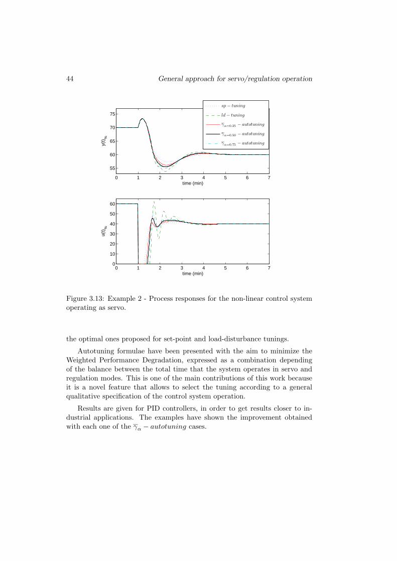
A more comprehensive picture of the process outputs, for the set-pointchange, is shown in Fig. 3.13. In this case, it can be seen that, as expected,the set-point tuning gives the better performance for servo operation mode.Furthermore, the γα − autotuning provides a lower degradation, respect tothe optimal, than the load-disturbance tuning.
The detail of load-disturbance attenuation is in Fig. 3.14. Similarly tothe previous case, the load-disturbance tuning is the one that gives betterperformance for regulation operation and the performance degradation of theset-point tuning is greater than the three cases for γα − autotuning.
In general terms, it can be confirmed that the γα − autotuning gives abetter overall performance when the system operates in both servo and regu-lation modes. Also, the control signal for the intermediate tuning seems to besmoother than that provided by the optimal regulation settings.
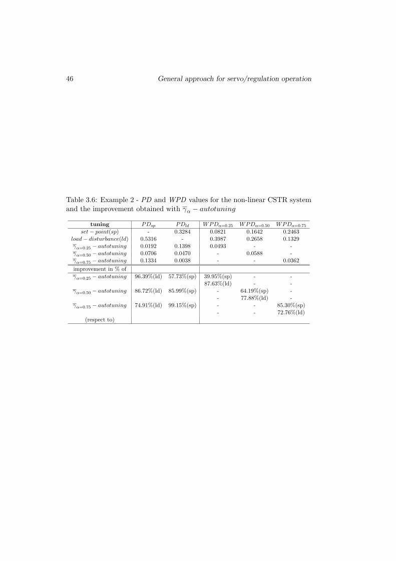
Table 3.6 shows the PD and WPD indices and the improvement that canbe achieve for each case of the γα − autotuning.
3.8 Summary 43
0 5 10 15 20 25 30
55
60
65
70
75
time (min)
y(t)
%
0 5 10 15 20 25 300
20
40
60
80
100
time (min)
u(t)
%
sp − tuning
ld − tuning
γα=0.25 − autotuning
γα=0.50 − autotuning
γα=0.75 − autotuning
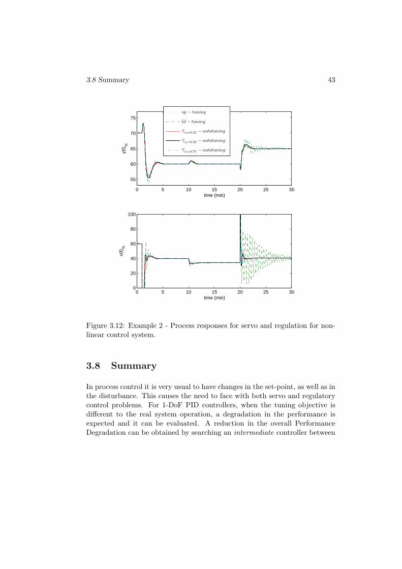
Figure 3.12: Example 2 - Process responses for servo and regulation for non-linear control system.
3.8 Summary
In process control it is very usual to have changes in the set-point, as well as inthe disturbance. This causes the need to face with both servo and regulatorycontrol problems. For 1-DoF PID controllers, when the tuning objective isdifferent to the real system operation, a degradation in the performance isexpected and it can be evaluated. A reduction in the overall PerformanceDegradation can be obtained by searching an intermediate controller between
44 General approach for servo/regulation operation
0 1 2 3 4 5 6 7
55
60
65
70
75
time (min)
y(t)
%
0 1 2 3 4 5 6 70
10
20
30
40
50
60
time (min)
u(t)
%sp − tuning
ld − tuning
γα=0.25 − autotuning
γα=0.50 − autotuning
γα=0.75 − autotuning
Figure 3.13: Example 2 - Process responses for the non-linear control systemoperating as servo.
the optimal ones proposed for set-point and load-disturbance tunings.
Autotuning formulae have been presented with the aim to minimize theWeighted Performance Degradation, expressed as a combination dependingof the balance between the total time that the system operates in servo andregulation modes. This is one of the main contributions of this work becauseit is a novel feature that allows to select the tuning according to a generalqualitative specification of the control system operation.
Results are given for PID controllers, in order to get results closer to in-dustrial applications. The examples have shown the improvement obtainedwith each one of the γα − autotuning cases.

3.8 Summary 45
9 10 11 12 13 14 1559.8
60
60.2
60.4
60.6
60.8
61
time (min)
y(t)
%
9 10 11 12 13 14 15
30
32
34
36
38
40
time (min)
u(t)
%
sp − tuning
ld − tuning
γα=0.25 − autotuning
γα=0.50 − autotuning
γα=0.75 − autotuning
Figure 3.14: Example 2 - Process responses for the non-linear control systemoperating as regulator
Even if the results were presented and exemplified using the ISE perfor-mance criteria, it could be possible to reproduce a similar methodology forother PID controller tuning, like the one that uses derivative action just ap-plied to the process output, or to other PID tunings with different performanceobjectives.
46 General approach for servo/regulation operation
Table 3.6: Example 2 - PD and WPD values for the non-linear CSTR systemand the improvement obtained with γα − autotuning
tuning PDsp PDld WPDα=0.25 WPDα=0.50 WPDα=0.75
set − point(sp) - 0.3284 0.0821 0.1642 0.2463load − disturbance(ld) 0.5316 - 0.3987 0.2658 0.1329γα=0.25 − autotuning 0.0192 0.1398 0.0493 - -γα=0.50 − autotuning 0.0706 0.0470 - 0.0588 -γα=0.75 − autotuning 0.1334 0.0038 - - 0.0362
improvement in % of
γα=0.25 − autotuning 96.39%(ld) 57.73%(sp) 39.95%(sp) - -87.63%(ld) - -
γα=0.50 − autotuning 86.72%(ld) 85.99%(sp) - 64.19%(sp) -- 77.88%(ld) -
γα=0.75 − autotuning 74.91%(ld) 99.15%(sp) - - 85.30%(sp)- - 72.76%(ld)
(respect to)

Chapter 4
Application to unstable andintegrating processes
4.1 Considerations
Much of the effort in control systems has been concentrated on the applicationto stable systems, while quite a few of the important chemical processing unitsin industrial and chemical practices are open-loop unstable processes that areknown to be difficult to control, especially when there exists a time delay,such as in the case of continuous stirred tank reactors, polymerization reactorsand bio-reactors which are inherently open-loop unstable by design (Sree andChidambaram, 2006).
Clearly, the tuning of controllers to stabilize these processes and to achieveadequate disturbance rejection is critical. Moreover, integrating processes arevery frequently encountered in process industries and many researchers havesuggested that for the purpose of designing a controller, a large number ofchemical processes could be modelled using an integrating process with timedelay. Consequently, there has been much interest in the literature in thetuning of industrially standard PID controllers for open-loop unstable systemsas well as for integrating processes.
In fact, several papers can be found in the literature that deals with thetuning of unstable (Lee et al., 2000; Visioli, 2001; Sree et al., 2004; Vivekand Chidambaram, 2005; Panda, 2009) and integrating processes (Lee et al.,
47
48 Application to unstable and integrating processes
2000; Visioli, 2001; Chen and Seborg, 2002; Chidambaram and Sree, 2003; Aliand Majhi, 2010). There is, however, a common problem with the tuningof PI/PID controllers for such systems: the tunings are usually devoted tothe servo or regulation operation and may exhibit a significant performancedegradation when operating on the tuning mode they were not designed for.This is also observed when operating with stable systems, but becomes re-ally a problem for unstable and integrating processes. A simple look at theexisting literature shows that the performance is highly dependent of usingthe appropriate tuning mode. (O’Dwyer, 2003) presents a collection of tuningrules for PID controllers for stable, unstable and integrating processes.
Based on this observation, in this chapter the purpose is to provide analternative way of addressing the tuning of unstable and integral processes inorder to alleviate the aforementioned situation and to provide a better overallperformance. The approach constitutes and extension of the method presentedin section 3.6 for stable systems (Arrieta et al., 2010). The idea is to find anintermediate tuning for the controller that improves the overall performance ofthe system, considered as a trade-off between servo and regulation operationmodes. The settings are determined from the combination of the optimal onesfor set-point and load-disturbance, presented in (Visioli, 2001), and takinginto account the balance between the importance of each one of the operationmodes for the control system (servo or regulation).
4.2 General framework
We consider again the unity-feedback system shown in Fig. 2.1, where P isan unstable system assumed to be modelled by
P (s) =K
Ts − 1e−Ls (4.1)
or if we have an integrating process, the model will be
P (s) =K
se−Ls (4.2)
In both cases, K is the process gain and L is the dead-time. For unsta-ble system (4.1), T is the time constant. These models are commonly used
4.3 Tuning rules for unstable processes 49
because are capable of satisfactorily modelling the dynamics of unstable andintegrating processes.
Let us consider for controller C, the ideal One-Degree-of-Freedom (1-DoF)PID controller, that is considered as
C(s) = Kp
(
1 +1
Tis+ Tds
)
(4.3)
where Kp is the proportional gain and Ti and Td are the integral and derivativetime constants, respectively.
The analysis presented here, is an extension of the Performance Degrada-tion idea, adapting all the aspects and considerations to the cases of unsta-ble an integrating systems. We rely once more on the Integral Square Error(ISE) criteria (2.6). In this case the settings are determined from a combi-nation of the optimal ones for set-point and load-disturbance, presented in(Visioli, 2001), and taking into account the balance between the preference ofeach one of the operation modes for the control system.
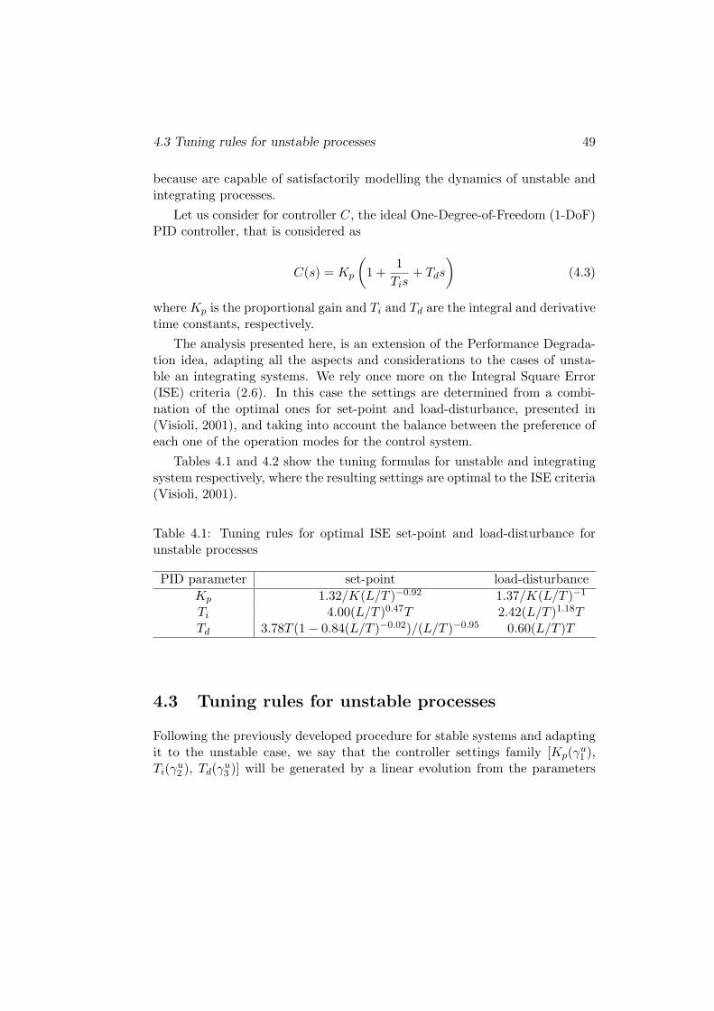
Tables 4.1 and 4.2 show the tuning formulas for unstable and integratingsystem respectively, where the resulting settings are optimal to the ISE criteria(Visioli, 2001).
Table 4.1: Tuning rules for optimal ISE set-point and load-disturbance forunstable processes
PID parameter set-point load-disturbance
Kp 1.32/K(L/T )−0.92 1.37/K(L/T )−1
Ti 4.00(L/T )0.47T 2.42(L/T )1.18TTd 3.78T (1 − 0.84(L/T )−0.02)/(L/T )−0.95 0.60(L/T )T
4.3 Tuning rules for unstable processes
Following the previously developed procedure for stable systems and adaptingit to the unstable case, we say that the controller settings family [Kp(γ
u1 ),
Ti(γu2 ), Td(γ
u3 )] will be generated by a linear evolution from the parameters

50 Application to unstable and integrating processes
Table 4.2: Tuning rules for optimal ISE set-point and load-disturbance forintegrating processes
PID parameter set-point load-disturbance
Kp 1.03/KL 1.37/KLTi - 1.49LTd 0.49L 0.29L
for the set-point tuning to the load-disturbance one and the other way around(as relations (3.7)). Therefore,
Kp(γu1 ) = γu
1 K ldp + (1 − γu
1 )Kspp
Ti(γu2 ) = γu
2 T ldi + (1 − γu
2 )T spi (4.4)
Td(γu3 ) = γu
3 T ldd + (1 − γu
3 )T spd
Once again, repeating the problem optimization posed in (3.21) for thethree weighting factors and different values of the normalized dead-time τ =L/T , we can find an optimal set for each γu
i parameter. For each one ofthese groups, it is possible to approximate a function to determine a generalprocedure that allows to find the suitable values for the γu
i ’s, that provide thebest intermediate tuning. Results are adjusted according to
γui (τ) = au + buτ + cuτ2 (4.5)
where au, bu and cu are given in Table 4.3, according to the weighting factorα and for each γu
i .
Equation (4.5) for each γui along with the settings (4.4) provide what we call
here γuα − tuning for unstable processes offering a weighted servo/regulation
operation.
4.3.1 Illustrative example
Consider the following unstable system represented by
P4(s) =1
s − 1e−0.2s (4.6)

4.4 Tuning rules for integrating processes 51
Table 4.3: γuα-tuning settings for unstable systems
α = 0.25 α = 0.50 α = 0.75
constant au bu cu au bu cu au bu cu
γu1 0.544 -1.631 2.194 0.629 -0.801 1.009 0.711 0.061 -0.324
γu2 0.807 0.100 -1.491 0.787 1.026 -2.513 0.687 2.173 -4.026
γu3 0.660 -0.019 0.293 0.718 0.268 -0.580 0.547 1.265 -2.116
The application of the ISE tuning formulae of (Visioli, 2001), as well as,the γu
α − tuning, provides the PID parameters shown in Table 4.4. Fig. 4.1shows the control system performance for the two possible operation modesfor the above tuning methods.
Table 4.4: Unstable process - PID controller parameters for P4
tuning Kp Ti Td
set − point(sp) 5.803 1.877 0.109load − disturbance(ld) 6.850 0.362 0.120
γuα=0.25 − tuning 6.123 0.715 0.116
γuα=0.50 − tuning 6.336 0.526 0.117
γuα=0.75 − tuning 6.547 0.442 0.117
It can be seen that the proposed γuα − tuning gives lower performance
than the optimum settings when the system operates in the same way as itwas tuned. However, higher performance can be obtained for the whole sys-tem operation (regulatory-control and servo-control), when the intermediatecontroller is used.
Table 4.5 shows the PD and WPD indices and the improvement, in per-centage, that can be achieve for each case of the γu
α − tuning respect to theextreme tunings (set-point and load-disturbance).
4.4 Tuning rules for integrating processes
Now, we analyze the case for integrating systems represented as (4.2). For thiscase, it must be taken into account that the method presented in (Visioli, 2001)

52 Application to unstable and integrating processes
0 2 4 6 80
0.5
1
1.5
2
2.5
time
Pro
cess
Out
put
servo
sp − tuningld − tuningγu
α=0.25 − tuningγu
α=0.50 − tuningγu
α=0.75 − tuning
0 2 4 6 8−0.1
−0.05
0
0.05
0.1
0.15
0.2
0.25
0.3
time
Pro
cess
Out
put
regulation
sp − tuningld − tuningγu
α=0.25 − tuningγu
α=0.50 − tuningγu
α=0.75 − tuning
Figure 4.1: Unstable process - Servo and regulation control responses for sys-tem P4.
Table 4.5: Unstable process - PD and WPD values for the system P4 and theimprovement obtained with γu
α − tuning.
tuning PDsp PDld WPDα=0.25 WPDα=0.50 WPDα=0.75
set − point(sp) - 1.8829 0.4707 0.9414 1.4122load − disturbance(ld) 0.6788 - 0.5091 0.3394 0.1697
γuα=0.25 − tuning 0.1207 0.3190 0.1703 - -
γuα=0.50 − tuning 0.2524 0.0993 - 0.1759 -
γuα=0.75 − tuning 0.4201 0.0088 - - 0.1116
improvement in % of
γuα=0.25 − tuning 82.21%(ld) 83.06%(sp) 63.82%(sp) - -
66.55%(ld) - -γu
α=0.50 − tuning 62.81%(ld) 94.73%(sp) - 81.32%(sp) -- 48.18%(ld) -
γuα=0.75 − tuning 38.10%(ld) 99.54%(sp) - - 92.10%(sp)
- - 34.23%(ld)(respect to)
uses a PD (Proportional-Derivative) controller, when the expected operationfor the system is servo-control. This kind of controller could be seen as a PIDcontroller with the integral part disabled, that is equivalent to Ti → ∞.
Regarding to the above consideration, the generation of the controller’sparameters family like (4.4), has the difficulty to make a transition in the
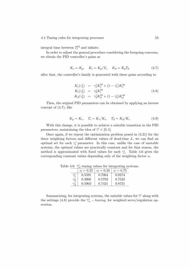
4.4 Tuning rules for integrating processes 53
integral time between T ldi and infinite.
In order to adjust the general procedure considering the foregoing concerns,we obtain the PID controller’s gains as
Kc = Kp, Ki = Kp/Ti, Kd = KpTd (4.7)
after that, the controller’s family is generated with these gains according to
Kc(γi1) = γi
1Kldc + (1 − γi
1)Kspc
Ki(γi2) = γi
2Kldi (4.8)
Kd(γi3) = γi
3Kldd + (1 − γi
3)Kspd
Then, the original PID parameters can be obtained by applying an inverseconcept of (4.7), like
Kp = Kc, Ti = Kc/Ki, Td = Kd/Kc (4.9)
With this change, it is possible to achieve a suitable transition in the PIDparameters, maintaining the idea of γi ∈ [0, 1].
Once again, if we repeat the optimization problem posed in (3.21) for thethree weighting factors and different values of dead-time L, we can find anoptimal set for each γi
i parameter. In this case, unlike the case of unstablesystems, the optimal values are practically constant and for that reason, themethod is approximated with fixed values for each γi
i . Table 4.6 gives thecorresponding constant values depending only of the weighting factor α.
Table 4.6: γiα-tuning values for integrating systems.α = 0.25 α = 0.50 α = 0.75
γi1 0.5591 0.7064 0.8274
γi2 0.3906 0.5702 0.7532
γi3 0.5903 0.7421 0.8731
Summarizing, for integrating systems, the suitable values for γi along withthe settings (4.8) provide the γi
α − tuning, for weighted servo/regulation op-eration.

54 Application to unstable and integrating processes
0 50 100 1500
0.5
1
1.5
2
2.5
time
Pro
cess
Out
put
servo
sp − tuningld − tuningγi
α=0.25 − tuning
γiα=0.50 − tuning
γiα=0.75 − tuning
0 50 100 150−0.1
−0.05
0
0.05
0.1
0.15
0.2
0.25
0.3
0.35
time
Pro
cess
Out
put
regulation
sp − tuningld − tuningγi
α=0.25 − tuningγi
α=0.50 − tuning
γiα=0.75 − tuning
Figure 4.2: Integrating process - Servo and regulation control responses forsystem P5.
4.4.1 Illustrative example
Consider the following integrating process represented by
P5(s) =0.0506
se−6s (4.10)
Table 4.7 shows the PID controller parameters for the system (4.10) us-ing the (Visioli, 2001) method and the proposed γi
α − tuning with α ={0.25, 0.50, 0.75}. Fig. 4.1 shows the control system output for the servoand regulation operation modes.
Table 4.7: Integrating process - PID controller parameters for P5
tuning Kp Ti Td
set − point(sp) 3.393 - 2.940load − disturbance(ld) 4.513 8.940 3.540
γiα=0.25 − tuning 4.019 20.384 3.363
γiα=0.50 − tuning 4.184 14.536 3.448
γiα=0.75 − tuning 4.319 11.361 3.552

4.5 Comparative Study 55
It can be confirmed that the γiα − tuning gives a better performance when
the system operates in both servo and regulation modes. Special attention hasto be put to the set-point tuning operating in regulation mode because beingthe controller PD type (without integral action), a static error is expected andconsequently the Performance Degradation is infinite.
Table 4.8 shows the PD and WPD indices and the improvement, that canbe achieve for each case of the γi
α − tuning.
Table 4.8: Integrating process - PD and WPD values for the system P5 andthe improvement obtained with γi
α − tuning.
tuning PDsp PDld WPDα=0.25 WPDα=0.50 WPDα=0.75
set − point(sp) - ∞ ∞ ∞ ∞load − disturbance(ld) 0.9742 - 0.7307 0.4871 0.2436
γiα=0.25 − tuning 0.2810 0.4611 0.3260 - -
γiα=0.50 − tuning 0.4443 0.1682 - 0.3063 -
γiα=0.75 − tuning 0.6393 0.0468 - - 0.1950
improvement in % of
γiα=0.25 − tuning 71.16%(ld) ∞(sp) ∞(sp) - -
55.38%(ld) - -γi
α=0.50 − tuning 54.39%(ld) ∞(sp) - ∞(sp) -- 37.12%(ld) -
γiα=0.75 − tuning 34.38%(ld) ∞(sp) - - ∞(sp)
- - 19.95%(ld)(respect to)
4.5 Comparative Study
In this section the proposed γα − tuning method with α = 0.50 (balancedservo and regulation operation) is compared with other well known PID tuningmethods for unstable and integrating systems.
4.5.1 Unstable process example
Let us consider the First-Order-Delayed-Unstable-Process (FODUP) with thefollowing transfer function

56 Application to unstable and integrating processes
0 15 30 45 600
0.5
1
1.5
2
2.5
3
time
Pro
cess
Out
put
servo
γu
α=0.50 − tuningPanda (2009)Sree et al. (2004)Lee et al. (2000)
0 15 30 45 60−1
−0.5
0
0.5
1
1.5
2
2.5
3
3.5
4
timeP
roce
ss O
utpu
t
regulation
γu
α=0.50 − tuningPanda (2009)Sree et al. (2004)Lee et al. (2000)
Figure 4.3: Unstable process - Servo and regulation control responses for sys-tem P6.
P6(s) =4
4s − 1e−2s (4.11)
Table 4.9 shows the PID parameters obtained with different tuning meth-ods for system (4.11). Also in Fig. 4.3 it is possible to see the process outputsfor the servo and regulation cases.
Table 4.9: Unstable process - PID controller parameters for P6
tuning Kp Ti Td
γuα=0.50 − tuning 0.654 6.662 1.188(Panda, 2009) 0.653 10.420 0.908
(Sree et al., 2004) 0.571 11.122 1.025(Lee et al., 2000)(λ = L) 0.606 11.732 0.840
Table 4.10 gives the performance criteria (3.1) for servo (Jsp) and regula-tion (Jld) operation modes, as well as, the associated Performance Degradationindices ((3.17) to (3.20)) for each tuning.
All the values confirm the fact that, in global terms, when both operatingmodes could appear and taking into account the importance that the control-

4.5 Comparative Study 57
Table 4.10: Unstable process - Performance and Performance Degradationindices for system P6.
tuning Jsp Jld PDsp1 PDld
2 WPDα=0.50
γuα=0.50 − tuning 8.9776 26.3352 0.0837 0.0728 0.0783(Panda, 2009) 9.2178 34.3572 0.1127 0.3997 0.2562
(Sree et al., 2004) 9.4747 46.7897 0.1437 0.9061 0.5249(Lee et al., 2000)(λ = L) 9.9005 44.4132 0.1951 0.8093 0.5022
1 Calculated using equation (3.17) with Jsp(sp) = 8.2839.2 Calculated using equation (3.18) with Jld(ld) = 24.5470.
loop is operating as servo or regulation mode, the proposed γuα − tuning is
the best choice to tune the PID controller in order to get less PerformanceDegradations.
4.5.2 Integrating process example
A distillation column separates a small amount of a low-boiling material fromthe final product. This technique is very common in chemical processes forthe separation of mixed fluids. The bottom level of the distillation column iscontrolled by adjusting the steam flow rate. The process for the level controlsystem is usually represented by an integrating model as
P7(s) =0.2
se−7.4s (4.12)
The PID controller parameters, for the different tuning methods, are shownin Table 4.11 and in Fig. 4.4 there are the process outputs for system (4.12)operating in servo and regulation modes.
In Table 4.12, there are the performance criteria (3.1) for servo (Jsp)and regulation (Jld) operation modes, as well as, the associated PerformanceDegradation indices ((3.17) to (3.20)) for each tuning.
From all the data, it is possible to see that even that the servo performanceof the proposed tuning is lower than the provided for the other tunings, thegeneral behavior (taking into account both operation modes) of the controlsystem, tuned with γi
α − tuning, is better. This means achieving the bestvalue for the Weighted Performance Degradation index (WPD).

58 Application to unstable and integrating processes
Table 4.11: Integrating process - PID controller parameters for P7
tuning Kp Ti Td
γiα=0.50 − tuning 0.858 17.928 4.253
(Ali and Majhi, 2010) 0.696 23.458 3.626(Chidambaram and Sree, 2003) 0.834 33.300 3.330
(Lee et al., 2000)(λ = L) 0.675 27.099 2.620
0 50 100 150 2000
0.2
0.4
0.6
0.8
1
1.2
1.4
1.6
1.8
time
Pro
cess
Out
put
servo
γi
α=0.50 − tuningAli and Maijhi (2010)Chidambaram and Sree (2003)Lee et al. (2000)
0 50 100 150 200−0.2
0
0.2
0.4
0.6
0.8
1
1.2
1.4
1.6
1.8
time
Pro
cess
Out
put
regulation
γi
α=0.50 − tuningAli and Maijhi (2010)Chidambaram and Sree (2003)Lee et al. (2000)
Figure 4.4: Integrating process - Servo and regulation control responses forsystem P7.
Table 4.12: Integrating process - Performance and Performance Degradationindices for system P7.
tuning Jsp Jld PDsp1 PDld
2 WPDα=0.50
γiα=0.50 − tuning 14.4299 22.4365 0.4443 0.1684 0.3063
(Ali and Majhi, 2010) 13.0946 36.8297 0.3106 0.9179 0.6142(Chidambaram and Sree, 2003) 12.3686 33.7810 0.2380 0.7591 0.4985
(Lee et al., 2000)(λ = L) 13.3858 44.9949 0.3398 1.3430 0.8414
1 Calculated using equation (3.17) with Jsp(sp) = 9.9912.2 Calculated using equation (3.18) with Jld(ld) = 19.2036.

4.6 Summary 59
4.6 Summary
The control of stable processes by using PI/PID controllers is by now a wellestablished and understood problem (even new methods and approaches arecontinuously appearing). However, when the process has integrating or unsta-ble characteristics the problem becomes much more difficult. Several proposalshave appeared in the literature presenting different approaches to tackle theproblem
These procedures are usually related to servo or regulation control prob-lems, however, in process control it is very usual to have changes in the set-point as well as in the disturbance. A common drawback of such approachesis the high loss of performance if the other operation mode is used.
An approach for providing a unique tuning for unstable and integratingprocesses, depending on the importance given to the system operations inservo and regulation modes, is presented. It combines tunings for both op-eration modes in such a way that the performance degradation is traded-off.Results are given for PID controllers, in order to get results closer to indus-trial applications and the examples have shown the improvement that can beachieved with the proposal.

60 Application to unstable and integrating processes

Part II
Robustness and performancetrade-off for PID controllers
61

Chapter 5
Robust based PID controldesign
5.1 Motivation and framework
Robustness is an important attribute for control systems, because the designprocedures are usually based on the use of low-order linear models identifiedat the closed-loop operation point. Due to the non-linearity found in mostof the industrial process, it is necessary to consider the expected changesin the process characteristics assuming certain relative stability margins, orrobustness requirements, for the control system. Therefore, the design of theclosed-loop control system must take into account the system performance toload-disturbance and set-point changes and its robustness to variation of thecontrolled process characteristics, preserving the well-known trade-off betweenall these variables.
The general procedure, presented in chapter 3, depends on a direct way ofthe extreme tunings, robustness considerations are therefore not taken into ac-count explicitly. Of course, if the original extreme tunings include any closed-loop characteristic, for example stability or robustness, they would be reflectedin the resulting intermediate tuning. In this sense, the purpose here is to goforward and to propose an approach that takes into account the robustnessissue, in an explicit way at the design stage.
Another aspect that is constrained by the extreme tunings is the PIDcontroller type. On this direction, it is desirable to use a PID controller
63

64 Robust based PID control design
that applies the derivative part just to the feedback signal, in order to avoidextreme instantaneous change in the controller output signal when a set-pointstep change occurs (Astrom and Hagglund, 2006). This kind of controller iscommonly called ISA-PID and it is the most dominating control structurepresent in industrial control applications.
Taking into account the above statements, we consider the feedback controlsystem shown in Fig. 5.1, where P (s) is the controlled process, C(s) is thecontroller, r(s) is the set-point, u(s) is the controller output signal, d(s) is theload-disturbance and y(s) is the system output.
) ( s C ) ( s P +
+ ) ( s r ) ( s y
) ( s d
) ( s u
Figure 5.1: Closed-loop control system.
Now, the output of the ISA-PID controller is given by
u(s) = Kp
(
1 +1
Tis
)
e(s) − Kp
(Tds
1 + (Td/N)s
)
y(s) (5.1)
where e(s) = r(s)−y(s) is the control error, Kp is the controller static gain, Ti
the integral time constant, Td the derivative time constant and the derivativefilter constant N is taken N = 10 as it is usual practice in industrial controllers.
5.1.1 Performance
One way to evaluate the performance of control systems is by calculating a costfunction based on the error, i.e. the difference between the desired value (set-point) and the actual value of the controlled variable (system’s output). Ofcourse, as larger and longer in time is be the error, the system’s performancewill be worse.

5.1 Motivation and framework 65
In this sense, a common reference for the evaluation of the controller per-formance, is a functional based on the integral of the error like: Integral-Square-Error (ISE) (2.6), or Integral-Absolute-Error (IAE).
Some approaches had used the ISE criterion, because its definition allowsan analytical calculation for the index (Zhuang and Atherton, 1993; Visioli,2001). However, nowadays can be found in the literature that IAE is the mostuseful ans suitable index to quantify the performance of the system (Chen andSeborg, 2002; Skogestad, 2003; Astrom and Hagglund, 2006; Kristiansson andLennartson, 2006; Tan et al., 2006). It can be used explicitly in the designstage or just as an evaluation measure.
The formulation of the criterion is stated as
IAE.=
∫∞
0|e(t)| dt =
∫∞
0|r(t) − y(t)| dt (5.2)
where the index can be measure for changes in the set-point or in the load-disturbance.
5.1.2 Robustness
As an indication of the system robustness (relative stability) the SensitivityFunction peak value will be used. The control system Maximum Sensitivity isdefined as
Ms.= max
ω|S(jω)| = max
ω
1
|1 + C(jω)P (jω)|(5.3)
and recommended values for Ms are typically within the range 1.4 - 2.0(Astrom and Hagglund, 2006).
The use of the maximum sensitivity as a robustness measure, has the ad-vantage that lower bounds to the Gain, Am, and Phase, φm, margins (Astromand Hagglund, 2006) can be assured according to
Am >Ms
Ms − 1
φm > 2 sin−1
(1
2Ms
)

66 Robust based PID control design
Therefore, to assure Ms = 2.0 provides what is commonly considered min-imum robustness requirement (that translates to Am > 2 and φm > 29o, forMs = 1.4 we have Am > 3.5 and φm > 41o).
5.2 Optimization problem formulation
From the above definitions for performance and robustness specifications, thereappears the need to formulate a joint criteria that faces with the trade-offbetween the performance for servo and regulation operation and also thattakes into account the accomplishment of a robustness level.
5.2.1 Servo/Regulation trade-off
As it was exposed before, there is a trade-off behavior between the dynamicsfor servo and regulation control operation modes. It is not enough just toconsider the tuning mode, it is also necessary to include the system operationin the controller’s design.
Using some of the exposed ideas, we can say that Jzx represents the criteria
(5.2) taking into account the operation mode x, for a tuning mode z. Fromthis, we can post the following definitions:
• Jrr is the value of performance index for the set-point tuning operating
in servo-control mode.
• Jrd is the value of performance index for the set-point tuning operating
in regulatory-control mode.
• Jdr is the value of performance index for the load-disturbance tuning
operating in servo-control mode.
• Jdd is the value of performance index for the load-disturbance tuning
operating in regulatory-control mode.
Obviously Jrr is the optimal value for servo-control operation, Jo
r , and Jdd is
the optimal one for regulation, Jod . An intermediate tuning between servo and
regulation operation modes should have higher values than the optimal ones,when the tuning and operation modes are the same, but the indexes would be

5.2 Optimization problem formulation 67
lower when the modes are different. So, for each operation mode we have thefollowing relationships,
Jor
.= Jr
r ≤ Jrdr ≤ Jd
r
Jod
.= Jd
d ≤ Jrdd ≤ Jr
d
where Jrdr and Jrd
d are the performance values of the intermediate tuning forservo and regulation control operation, respectively.
The previous ideas can be represented graphically, the results are shownin Fig. 5.2, where the performance indexes are plotted in the Jr − Jd plane.
J d r J rd
r J r r
J rd d
J d d
J r d
J d
J r
Load-disturbance tuning
Set-point tuning
Intermediate
tuning
“Ideal”
point
Figure 5.2: Plane Jr − Jd.
It can be seen that the point (Jrr , Jd
d ) is the “ideal” one because it representsthe minimum performance values taking both possible operation modes, servoand regulation, into account. However, this point is unreachable due thedifferences in the dynamics for each of the objectives of the control operationmodes. Therefore our efforts must go towards getting the minimum resultingdistance, meaning the best balance between the operation modes.
On this way, a cost objective function is formulated in order to get closer,as much as possible, the resulting point (Jrd
r , Jrdd ), to the “ideal” one, (Jo
r , Jod ).
Therefore,

68 Robust based PID control design
Jrd =
√
(Jrdr − Jo
r )2+
(Jrd
d − Jod
)2(5.4)
where Jor and Jo
d are the optimal values for servo and regulation control respec-tively, and Jrd
r , Jrdd are the performance indexes for the intermediate tuning
considering both operation modes. In Fig. 5.2, index (5.4) is represented bythe arrow between the “ideal” point and the corresponding to the intermediatetuning.
From the above analysis, the optimization problem setup considers themodel’s normalized dead-times, τ , in the range 0.1 ≤ τ ≤ 2.0, to obtain thePID controller optimum parameters such that
po := [Kpo, Tio, Tdo] = arg
[
minp
Jrd
]
(5.5)
where p is the PID controller parameters vector. Here, optimization is doneusing genetic algorithms technique.
The aim of minimization (5.5) is to achieved a balanced performance forboth operation modes of the control system.
5.2.2 Robustness constraint criterion
The cost functional (5.4) proposed before, even though face with the trade-offproblem between the operation modes of the system, just takes into accountcharacteristics of performance. However, there is a need to include a certainrobustness for the control-loop.
In that sense, we want to use (5.3) as a robustness measure. So, theoptimization problem (5.5) is subject to a constraint of the form
|Ms − Mds | = 0 (5.6)
where Ms and Mds are the Maximum Sensitivity and the desired Maximum
Sensitivity functions respectively. This constraint tries to guarantee the se-lected robustness value for the control system.

5.3 Servo/regulation PID tunings with robustness consideration 69
5.3 Servo/regulation PID tunings with robustnessconsideration
From the previous formulation, we look for a tuning rule that face with thetrade-off problem between the performance for servo and regulation modesand providing, at the same time, a certain degree of robustness (if necessary).
5.3.1 PID tuning for specified robustness levels
As it has been stated, we solve the optimization problem (5.5) subject toconstraint (5.6). In that sense, a broad classification can be established, usingspecific values for Ms, within the suggested range between 1.4 − 2.0. Thiswill allow a qualitative specification for the control system robustness. So, therating can be described as
• Low robustness level - Ms = 2.0
• Medium-low robustness level - Ms = 1.8
• Medium-high robustness level - Ms = 1.6
• High robustness level - Ms = 1.4
According to this principle, the above mentioned four values for Ms areused here as desirable robustness, Md
s into the robustness constraint (5.6), forthe problem optimization (5.5). Additionally, an unconstrained optimizationis done, that can be seen as the Md
s free case.
In order to provide results for autotuning methodology, the optimal sets forthe PID parameters with the corresponding desired robustness, are approx-imated in equations for each controller’s parameter. This fitting procedurelooks for simple expressions that allow for an homogenized set, to preserve thesimplicity and completeness of the approach.
Therefore, the resulting controller parameters will be, expressed just interms of the FOPDT process model parameters (2.1) as
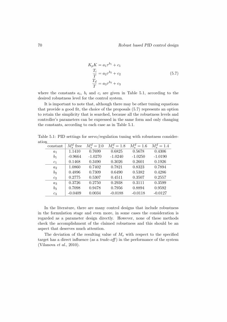
70 Robust based PID control design
KpK = a1τb1 + c1
Ti
T= a2τ
b2 + c2 (5.7)
Td
T= a3τ
b3 + c3
where the constants ai, bi and ci are given in Table 5.1, according to thedesired robustness level for the control system.
It is important to note that, although there may be other tuning equationsthat provide a good fit, the choice of the proposals (5.7) represents an optionto retain the simplicity that is searched, because all the robustness levels andcontroller’s parameters can be expressed in the same form and only changingthe constants, according to each case as in Table 5.1.
Table 5.1: PID settings for servo/regulation tuning with robustness consider-ation
constant Mds free Md
s = 2.0 Mds = 1.8 Md
s = 1.6 Mds = 1.4
a1 1.1410 0.7699 0.6825 0.5678 0.4306b1 -0.9664 -1.0270 -1.0240 -1.0250 -1.0190c1 0.1468 0.3490 0.3026 0.2601 0.1926
a2 1.0860 0.7402 0.7821 0.8323 0.7894b2 0.4896 0.7309 0.6490 0.5382 0.4286c2 0.2775 0.5307 0.4511 0.3507 0.2557
a3 0.3726 0.2750 0.2938 0.3111 0.3599b3 0.7098 0.9478 0.7956 0.8894 0.9592c3 -0.0409 0.0034 -0.0188 -0.0118 -0.0127
In the literature, there are many control designs that include robustnessin the formulation stage and even more, in some cases the consideration isregarded as a parameter design directly. However, none of these methodscheck the accomplishment of the claimed robustness and this should be anaspect that deserves much attention.
The deviation of the resulting value of Ms with respect to the specifiedtarget has a direct influence (as a trade-off ) in the performance of the system(Vilanova et al., 2010).
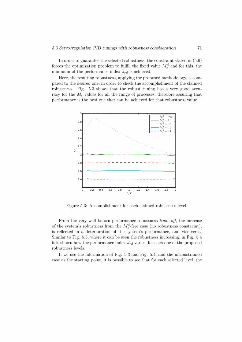
5.3 Servo/regulation PID tunings with robustness consideration 71
In order to guarantee the selected robustness, the constraint stated in (5.6)forces the optimization problem to fulfill the fixed value Md
s and for this, theminimum of the performance index Jrd is achieved.
Here, the resulting robustness, applying the proposed methodology, is com-pared to the desired one, in order to check the accomplishment of the claimedrobustness. Fig. 5.3 shows that the robust tuning has a very good accu-racy for the Ms values for all the range of processes, therefore assuring thatperformance is the best one that can be achieved for that robustness value.
0 0.2 0.4 0.6 0.8 1 1.2 1.4 1.6 1.8 2
1.4
1.6
1.8
2
2.2
2.4
2.6
2.8
3
L/T
Ms
Md
s − free
Mds = 2.0
Mds = 1.8
Mds = 1.6
Mds = 1.4
Figure 5.3: Accomplishment for each claimed robustness level.
From the very well known performance-robustness trade-off, the increaseof the system’s robustness from the Md
s -free case (no robustness constraint),is reflected in a deterioration of the system’s performance, and vice-versa.Similar to Fig. 5.3, where it can be seen the robustness increasing, in Fig. 5.4it is shown how the performance index Jrd varies, for each one of the proposedrobustness levels.
If we use the information of Fig. 5.3 and Fig. 5.4, and the unconstrainedcase as the starting point, it is possible to see that for each selected level, the

72 Robust based PID control design
0 0.2 0.4 0.6 0.8 1 1.2 1.4 1.6 1.8 20
0.5
1
1.5
L/T
Jrd
Md
s − free
Mds = 2.0
Mds = 1.8
Mds = 1.6
Mds = 1.4
Figure 5.4: Combined index Jrd for each robustness level tuning.
robustness is improved achieving smaller values for Ms, but at the same timehaving larger values (i.e worse) for the performance index Jrd.
It is also important to note that, the relation between the loss of perfor-mance and the robustness increase (for each level of Ms) is nonlinear, neitherfor the τ range. For example, in Fig. 5.4 the difference between the perfor-mance for cases Md
s = 1.8 and Mds = 1.6, is much lower than the one for
Mds = 1.6 and Md
s = 1.4, despite that the levels are equally separated.
In general terms, it is possible to say that the robustness requirements arefulfilled, facing at the same time, to the performance servo/regulation trade-offproblem.
5.3.2 PID tuning for an arbitrary specific robustness value
With the aim to give more completeness to the previous exposed tuningmethod, an extension of the approach is presented. We want to take ad-vantage of the simplicity and homogeneity offered by tuning (5.7), in order to

5.3 Servo/regulation PID tunings with robustness consideration 73
exploit in the same lines, for a simple tuning rule that allows to specify, on anexplicit way, the robustness parameter value within the range Ms ∈ [1.4, 2.0].
Maybe, it is true that from a more practical point of view, it is difficult tohave an specification of a Ms = 1.57 and this fact leads to the establishmentof qualitative levels. However, a generic Md
s tuning method can be used as acomparison tool, setting the same robustness (e.g. from a robust profile forall range of τ), and looking for the behavior of the performance.
Once again, the above idea is possible just because the followed fittingprocedure was conceived to have the same form for each tuning and also foreach parameter. Thus, the final expression for the controller’s parameters thatwe are looking for is
pi(τ, Mds ) = ai(M
ds )τ bi(M
ds ) + ci(M
ds ) (5.8)
where i = 1, 2, 3 indicates the corresponding controller’s parameter, p, andconstants are expressed as functions of Md
s . Therefore, from Table 5.1 eachconstant ai, bi and ci are generated from a a generic second order Md
s depen-dent polynomial as
a1 = −0.3112(Mds )2 + 1.6250(Md
s ) − 1.2340
b1 = 0.0188(Mds )2 − 0.0753(Md
s ) − 0.9509
c1 = −0.1319(Mds )2 + 0.7042(Md
s ) − 0.5334
a2 = −0.5300(Mds )2 + 1.7030(Md
s ) − 0.5511
b2 = −0.1731(Mds )2 + 1.0970(Md
s ) − 0.7700 (5.9)
c2 = −0.0963(Mds )2 + 0.7899(Md
s ) − 0.6629
a3 = 0.1875(Mds )2 − 0.7735(Md
s ) + 1.0740
b3 = 0.3870(Mds )2 − 4.7810(Md
s ) + 4.9470
c3 = 0.1331(Mds )2 − 0.4733(Md
s ) + 0.4032
Parameters (5.7) joint with (5.9) allow to determine the PID controller forany arbitrary value Md
s in the range [1.4, 2.0].
As it was said before, the accomplishment of the selected value for Ms is anaspect that must be checked. Fig. 5.5 shows the resulting Ms values obtainedwith the generic tuning (5.7) and (5.9), for the previously stated robustness
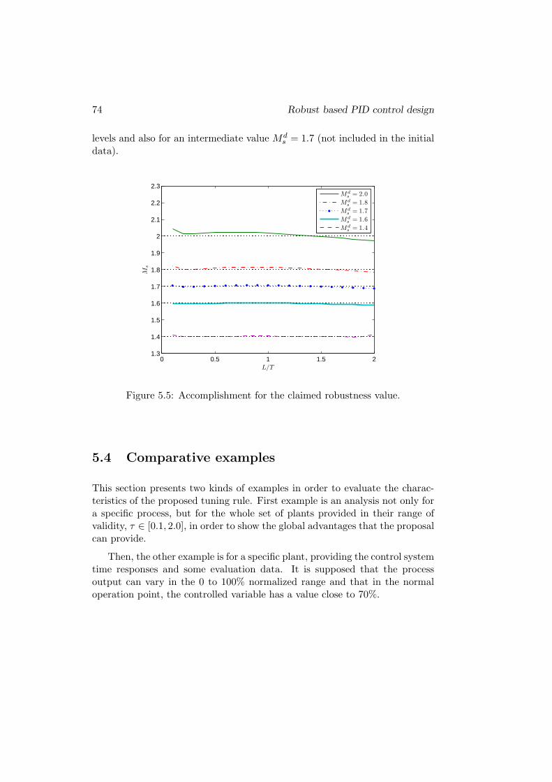
74 Robust based PID control design
levels and also for an intermediate value Mds = 1.7 (not included in the initial
data).
0 0.5 1 1.5 21.3
1.4
1.5
1.6
1.7
1.8
1.9
2
2.1
2.2
2.3
L/T
Ms
Md
s = 2.0
Mds = 1.8
Mds = 1.7
Mds = 1.6
Mds = 1.4
Figure 5.5: Accomplishment for the claimed robustness value.
5.4 Comparative examples
This section presents two kinds of examples in order to evaluate the charac-teristics of the proposed tuning rule. First example is an analysis not only fora specific process, but for the whole set of plants provided in their range ofvalidity, τ ∈ [0.1, 2.0], in order to show the global advantages that the proposalcan provide.
Then, the other example is for a specific plant, providing the control systemtime responses and some evaluation data. It is supposed that the processoutput can vary in the 0 to 100% normalized range and that in the normaloperation point, the controlled variable has a value close to 70%.

5.4 Comparative examples 75
5.4.1 Complete tuning case
The robust tuning rules that can be found in the literature consider differentspecifications for Ms. They range from the considered minimum robustness;Ms = 2.0; to a high robustness; Ms = 1.4.
Here, we compare the tuning proposed in Section 5.3 with the followingmethods:
• AMIGO method (Astrom and Hagglund, 2004) provides tuning with adesign specification of Ms = 1.4.
• Kappa-Tau (κ− τ) method (Astrom and Hagglund, 1995) provides tun-ing with a design specification of Ms = 1.4 and Ms = 2.0.
• Tavakoli method (Tavakoli et al., 2005) provides tuning with a designspecification of Ms = 2.0.
Fig. 5.6 shows the achieved Ms values for 1.4 and 2.0 cases, for the com-pared tuning rules. With this information and the one in Fig. 5.3, it seemsthat the proposed tuning is the option that provides the best accuracy for theselected robustness.
With the aim to establish a more precise and quantitative measure of theclaimed robustness accomplishment for the whole range of models, the nextindex is stated
IMs
.=
∫ τf
τo
|M rs (τ) − Md
s (τ)|dτ (5.10)
where Mds and M r
s are the desired and resulting Ms values, respectively. AsIMs is smaller, the accuracy is better. In Table 5.2 there are the values (5.10)for the analyzed tuning rules.
Now, from the plots in Figs. 5.3 and 5.6, and the measured values (5.10) inTable 5.2, it is possible to say that the proposed PID tuning (using the levelsclassification), is the one that provides the best accomplishment between thedesirable and the achieved robustness.

76 Robust based PID control design
0.5 1 1.5 21.2
1.25
1.3
1.35
1.4
1.45
1.5
1.55
1.6
L/T
Ms
Mds = 1.4
0.5 1 1.5 21.5
1.6
1.7
1.8
1.9
2
2.1
L/T
Ms
Mds = 2.0
Proposed (level)Tavakoliκ− τ
Proposed (level)AMIGOκ− τ
Figure 5.6: Comparative for claimed robustness.
Table 5.2: Claimed robustness accomplishment IMs for different tuning rulesTuning Md
s IMs
AMIGO 1.4 0.0634κ − τ 1.4 4.9672κ − τ 2.0 10.2377
Tavakoli 2.0 0.0519
1.4 0.0035Proposed 1.6 0.0066(levels) 1.8 0.0111
2.0 0.0186
Proposed 1.4 0.0054(generic) MAMIGO
s 0.0028 (MAMIGOs )
0.0628 (1.4)
Once the robustness accomplishment has been verified, it is important tosee the resulting performance for the compared tuning rules. Fig. 5.7 showsthe combined servo/regulation performance index (5.4).
For the Mds = 2.0 it is obvious that the proposed tuning is the one that
provides the best robustness accomplishment and at the same time, the bestachievable performance. However, for Md
s = 1.4 case, even the proposal is

5.4 Comparative examples 77
0 0.5 1 1.5 20
0.2
0.4
0.6
0.8
1
1.2
1.4
1.6
1.8
2
L/T
Jrd
Mds = 1.4
0 0.5 1 1.5 20
0.2
0.4
0.6
0.8
1
1.2
1.4
1.6
1.8
2
L/T
Jrd
Mds = 2.0
Proposed (level)AMIGOκ− τ
Proposed (level)Tavakoliκ− τ
Figure 5.7: Jrd index for the compared tuning rules.
more accurate for the claimed robustness, Fig. 5.7 shows that AMIGO tun-ing method has values slightly lower for Jrd index compared to the proposedtuning. Precisely, because AMIGO method does not fulfill the robustness re-quirements, having a somewhat lower robustness, is that it achieves betterresults for performance. This fact strongly confirms the importance of therelation between robustness and performance variations.
Generic PID tuning method (5.7) joint with (5.9) allows to determine thecontroller parameters for any value Md
s in the range [1.4, 2.0]. So, it can setflat profiles for robustness as, Md
s = 1.4 (similarly to the level classificationcase), or variable ones as functions like Md
s = fMs(τ) .
From the above and in order to have a fair comparison, we can take advan-tage of the generic PID tuning, reproducing a profile with the same robustnessthat AMIGO tuning provides, Md
s = MAMIGOs (τ). Then, for the same robust-
ness the idea is to look for the best performance. Fig. 5.8 shows the results.
It can be seen that the proposed generic tuning, is very accurate for the twoselected robustness profiles. If we compare the proposal in the two situations(levels and generic), for the Md
s = 1.4 the resulting performance is practicallythe same. However, the most interesting thing is when the generic tuning is setwith the AMIGO values (MAMIGO
s ). As said before, AMIGO provides slightlylower values for Jrd index when the comparison is with the specified robustnesslevels, but if we use the generic approach to have exactly the same robustness
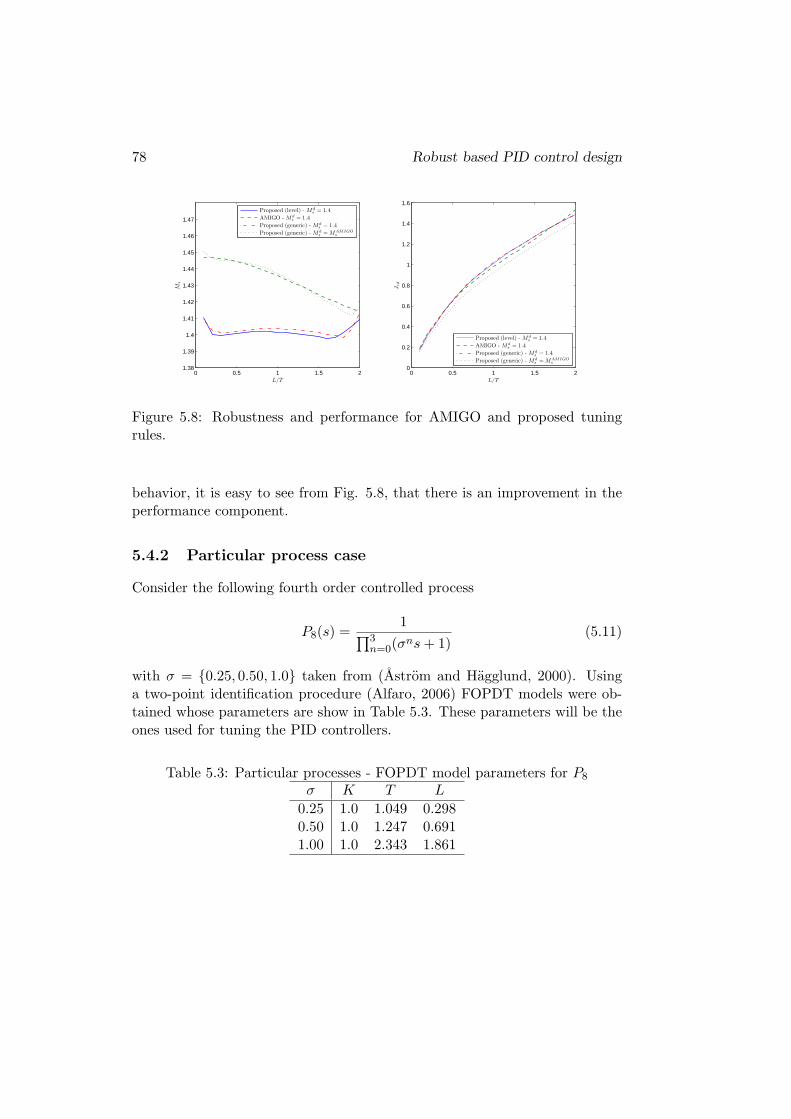
78 Robust based PID control design
0 0.5 1 1.5 21.38
1.39
1.4
1.41
1.42
1.43
1.44
1.45
1.46
1.47
L/T
Ms
Proposed (level) - Md
s = 1.4
AMIGO - Mds = 1.4
Proposed (generic) - Mds = 1.4
Proposed (generic) - Mds = MAMIGO
s
0 0.5 1 1.5 20
0.2
0.4
0.6
0.8
1
1.2
1.4
1.6
L/T
Jrd
Proposed (level) - Mds = 1.4
AMIGO - Mds = 1.4
Proposed (generic) - Mds = 1.4
Proposed (generic) - Mds = MAMIGO
s
Figure 5.8: Robustness and performance for AMIGO and proposed tuningrules.
behavior, it is easy to see from Fig. 5.8, that there is an improvement in theperformance component.
5.4.2 Particular process case
Consider the following fourth order controlled process
P8(s) =1
∏3n=0(σ
ns + 1)(5.11)
with σ = {0.25, 0.50, 1.0} taken from (Astrom and Hagglund, 2000). Usinga two-point identification procedure (Alfaro, 2006) FOPDT models were ob-tained whose parameters are show in Table 5.3. These parameters will be theones used for tuning the PID controllers.
Table 5.3: Particular processes - FOPDT model parameters for P8
σ K T L
0.25 1.0 1.049 0.2980.50 1.0 1.247 0.6911.00 1.0 2.343 1.861

5.4 Comparative examples 79
Table 5.4: Particular processes - PID controller parameters for P8σ = 0.25 σ = 0.50 σ = 1.00
Tuning Mds Kp Ti Td Kp Ti Td Kp Ti Td
AMIGO 1.4 1.784 0.709 0.137 1.012 1.079 0.296 0.767 2.326 0.751κ − τ 1.4 2.982 0.832 0.200 0.867 1.233 0.320 0.486 2.432 0.630κ − τ 2.0 5.712 0.654 0.165 1.719 1.151 0.285 1.030 2.555 0.633
1.4 1.745 0.751 0.100 0.978 1.083 0.239 0.737 2.274 0.646Proposed 1.6 2.323 0.811 0.094 1.300 1.193 0.215 0.979 2.544 0.566(levels) 1.8 2.779 0.836 0.094 1.552 1.227 0.206 1.167 2.635 0.529
2.0 3.153 0.866 0.091 1.761 1.261 0.200 1.324 2.709 0.523
Proposed 1.4 1.749 0.754 0.112 0.981 1.087 0.254 0.739 2.283 0.675(generic) MAMIGO
s 1.888 0.767 0.110 1.055 1.112 0.247 0.790 2.338 0.653
Table 5.5: Particular processes - Controller robustnessσ = 0.25 σ = 0.50 σ = 1.00
Tuning Mds M r
s |Mds − M r
s | M rs |Md
s − M rs | M r
s |Mds − M r
s |
AMIGO 1.4 1.446 0.046 (3.3%) 1.444 0.044 (3.1%) 1.440 0.040 (2.9%)κ − τ 1.4 2.922 1.522 (108.7%) 1.382 0.018 (1.3%) 1.234 0.166 (11.9%)κ − τ 2.0 12.370 10.370 (518.5%) 2.062 0.062 (3.1%) 1.655 0.345 (17.3%)
1.4 1.400 0.000 (0.0%) 1.401 0.001 (0.1%) 1.402 0.002 (0.1%)Proposed 1.6 1.598 0.002 (0.1%) 1.603 0.003 (0.2%) 1.605 0.005 (0.3%)(levels) 1.8 1.796 0.004 (0.2%) 1.804 0.004 (0.2%) 1.808 0.008 (0.4%)
2.0 1.995 0.005 (0.3%) 2.008 0.008 (0.4%) 2.013 0.013 (0.6%)
Proposed 1.4 1.401 0.001 (0.1%) 1.403 0.003 (0.2%) 1.404 0.004 (0.3%)(generic) MAMIGO
s 1.445 0.001 (0.1%) 1.444 0.000 (0.0%) 1.441 0.001 (0.1%)
Table 5.4 shows the PID controller parameters whereas in Table 5.5 thespecified (Md
s ) and achieved (M rs ) robustness of the control system, are pre-
sented when the controller is tuned with Kappa-Tau (κ − τ) (Astrom andHagglund, 1995) and AMIGO (Astrom and Hagglund, 2006) rules and thecorresponding parameters obtained with the proposed method (levels andgeneric). The accuracy in terms of |Md
s − M rs | is also shown, where it is
possible to say that, when qualitative robustness levels are specified, the pro-posed method is closer to the desired values than the AMIGO or Kappa-Tautuning rules.
The control system’s performance for servo Jr, regulation Jd and the com-bined index Jrd, are provided in Table 5.6 for each tuning and each case ofprocess P8.
The analysis to determine the best option to tune the controller, must be
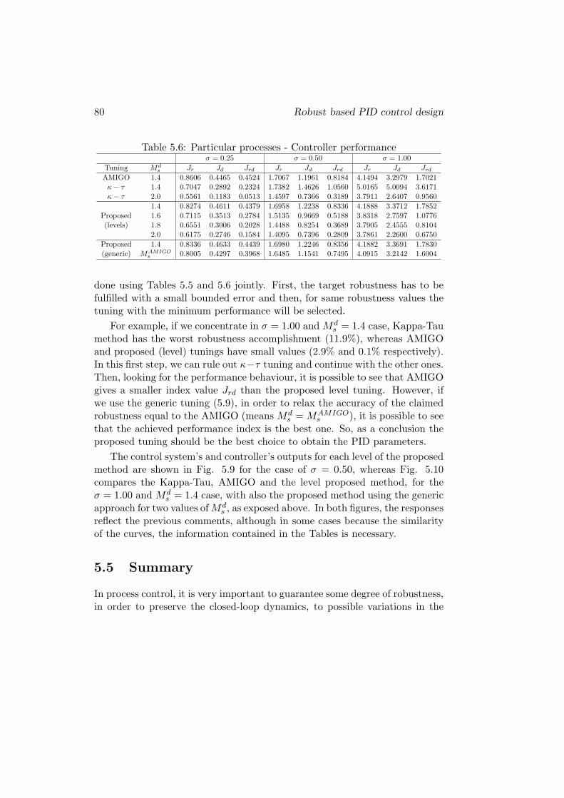
80 Robust based PID control design
Table 5.6: Particular processes - Controller performanceσ = 0.25 σ = 0.50 σ = 1.00
Tuning Mds Jr Jd Jrd Jr Jd Jrd Jr Jd Jrd
AMIGO 1.4 0.8606 0.4465 0.4524 1.7067 1.1961 0.8184 4.1494 3.2979 1.7021κ − τ 1.4 0.7047 0.2892 0.2324 1.7382 1.4626 1.0560 5.0165 5.0094 3.6171κ − τ 2.0 0.5561 0.1183 0.0513 1.4597 0.7366 0.3189 3.7911 2.6407 0.9560
1.4 0.8274 0.4611 0.4379 1.6958 1.2238 0.8336 4.1888 3.3712 1.7852Proposed 1.6 0.7115 0.3513 0.2784 1.5135 0.9669 0.5188 3.8318 2.7597 1.0776(levels) 1.8 0.6551 0.3006 0.2028 1.4488 0.8254 0.3689 3.7905 2.4555 0.8104
2.0 0.6175 0.2746 0.1584 1.4095 0.7396 0.2809 3.7861 2.2600 0.6750
Proposed 1.4 0.8336 0.4633 0.4439 1.6980 1.2246 0.8356 4.1882 3.3691 1.7830(generic) MAMIGO
s 0.8005 0.4297 0.3968 1.6485 1.1541 0.7495 4.0915 3.2142 1.6004
done using Tables 5.5 and 5.6 jointly. First, the target robustness has to befulfilled with a small bounded error and then, for same robustness values thetuning with the minimum performance will be selected.
For example, if we concentrate in σ = 1.00 and Mds = 1.4 case, Kappa-Tau
method has the worst robustness accomplishment (11.9%), whereas AMIGOand proposed (level) tunings have small values (2.9% and 0.1% respectively).In this first step, we can rule out κ−τ tuning and continue with the other ones.Then, looking for the performance behaviour, it is possible to see that AMIGOgives a smaller index value Jrd than the proposed level tuning. However, ifwe use the generic tuning (5.9), in order to relax the accuracy of the claimedrobustness equal to the AMIGO (means Md
s = MAMIGOs ), it is possible to see
that the achieved performance index is the best one. So, as a conclusion theproposed tuning should be the best choice to obtain the PID parameters.
The control system’s and controller’s outputs for each level of the proposedmethod are shown in Fig. 5.9 for the case of σ = 0.50, whereas Fig. 5.10compares the Kappa-Tau, AMIGO and the level proposed method, for theσ = 1.00 and Md
s = 1.4 case, with also the proposed method using the genericapproach for two values of Md
s , as exposed above. In both figures, the responsesreflect the previous comments, although in some cases because the similarityof the curves, the information contained in the Tables is necessary.
5.5 Summary
In process control, it is very important to guarantee some degree of robustness,in order to preserve the closed-loop dynamics, to possible variations in the

5.5 Summary 81
0 5 10 15 20 25 3070
75
80
85
time
y(t)
(%)
0 5 10 15 20 25 3060
70
80
90
100
time
u(t)
(%)
Md
s = 2.0
Mds = 1.8
Mds = 1.6
Mds = 1.4
Figure 5.9: Particular process - Proposed method (σ = 0.50).
control system. Also, at the same time, it must be provided the best achievableperformance for servo and regulation operation.
All of the above specifications, lead to have different trade-offs, betweenperformance and robustness or between servo and regulation modes, that mustbe solved on a balanced way. Here, we looked for a PID controller tuningrule that faces to the general problem. This tuning is optimal, as much aspossible, to a proposed performance index that takes into account both systemoperation modes, including also a certain degree of robustness, specified as adesirable Maximum Sensitivity value.
Autotuning formulae have been presented for two approaches. First, ro-bustness is established using a qualitative levels classification and then, theidea is extended to an issue that offers a generic expression, to allow the
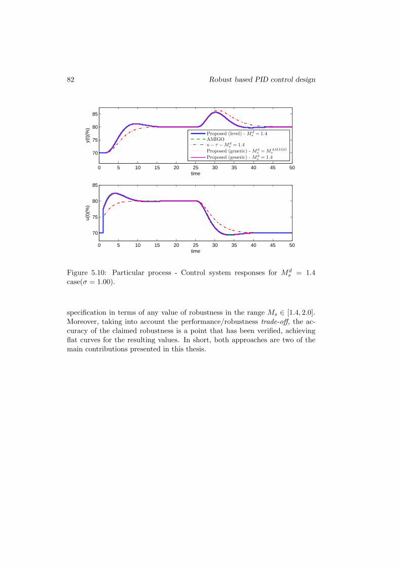
82 Robust based PID control design
0 5 10 15 20 25 30 35 40 45 50
70
75
80
85
time
y(t)
(%)
0 5 10 15 20 25 30 35 40 45 50
70
75
80
85
time
u(t)
(%)
Proposed (level) - Mds = 1.4
AMIGOκ− τ −Md
s = 1.4
Proposed (generic) - Mds = MAMIGO
s
Proposed (generic) - Mds = 1.4
Figure 5.10: Particular process - Control system responses for Mds = 1.4
case(σ = 1.00).
specification in terms of any value of robustness in the range Ms ∈ [1.4, 2.0].Moreover, taking into account the performance/robustness trade-off, the ac-curacy of the claimed robustness is a point that has been verified, achievingflat curves for the resulting values. In short, both approaches are two of themain contributions presented in this thesis.

Chapter 6
Optimality based PID controldesign
6.1 General aspects
The analysis exposed in Chapter 5, shows the interaction between performanceand robustness in control systems. It is possible to say that, an increase ofrobustness implies an optimality loss in the performance (i.e. a degradation),with respect to the one that can be achieved without any robustness constraint.From this,it is possible to define the degree of optimality of the constrainedcase, with respect to the unconstrained one (that is, the optimum).
In order to quantify the degree of optimality, the following index is pro-posed
IPerf.=
Jord
JrdMs
rd
(6.1)
where Jord is the optimal index value (5.4), using the tuning (5.7) for no con-
straint of Ms (first column of Table 5.1), that means the best one that canbe achieved. Then, JrdMs
rd is the value of index (5.4) for the cases where thetuning has a robustness constraint.
Note that (6.1) is normalized in the [0, 1] range, where IPerf = 1 means a
perfect optimality and, as much as the robustness is increased, the index JrdMs
rd
will increase and, consequently, IPerf < 1, meaning an optimality reduction.
83
84 Optimality based PID control design
The degree of optimality that each control system has when a desirablevalue of Ms is stated, can be evaluated taking advantage of the generic tuningrule presented before in section 5.3.2. For each value of Md
s ∈ [1.4 − 2.0], theoptimality degree (6.1) can be obtained.
Motivation example
In order to show how the optimality degree of a system varies, as a functionof the robustness variable Ms, a motivation example is provided.
Consider system (5.11), P8(s), with σ = 0.50, from the example in section5.4.2. For this particular process, the idea is to use each value within the rangeMd
s ∈ [1.4 − 2.0], as a design parameter of tuning (5.7) and (5.9). Then, itis possible to calculate a set of degree of optimality values (6.1) and comparethem with respect to the ones for AMIGO, Kappa-Tau and Tavakoli tuningmethods.
Fig. 6.1 illustrates the results, where it is shown the optimality indexIPerf with the corresponding achieved robustness. It is possible to see thatthe singletons for the compared tunings, are below the line that represents thegeneric proposed tuning for the Md
s range. This means that the proposal is theoption that provides better degree of optimality for any value of robustness.
In addition, note that the horizontal variation of the points representsthe error between the desired and the resulting robustness. The points forAMIGO, Kappa-Tau and Tavakoli methods, should be located on the axescorresponding to Ms = 1.4 and Ms = 2.0, but they are not, because they donot accomplish the robustness constraint.
The line for the proposed tuning, in Fig. 6.1, represents a limit. For eachchoice of robustness Md
s , the intersection point with the line, indicates the bestdegree of optimality that can be achieved. From the other side, if the choiceis a certain degree of optimality, the intersection provides the best robustnessvalue that can be selected.
This analysis has been done for one specific process (P8), however, the ideais to reproduce the same procedure in order to generalize the results for anypossible process.
From above, we want to repeat the idea of Fig. 6.1, but now for the wholerange of family plants within τ ∈ [0.1, 2.0]. So, for each τ , we take advantageof the possibilities of the proposed tuning (5.7) and (5.9), to get the PID

6.1 General aspects 85
1.3 1.4 1.5 1.6 1.7 1.8 1.9 2 2.10.2
0.3
0.4
0.5
0.6
0.7
0.8
0.9
Ms
I Perf
Proposed (generic) - Md
s ∈ [1.4, 2.0]
AMIGO - Mds = 1.4
κ− τ −Mds = 1.4
κ− τ −Mds = 2.0
TAVAKOLI - Mds = 2.0
Figure 6.1: Process P8 - Index IPerf values for different tunings.
parameters for any value of Mds ∈ [1.4 − 2.0] and then, compute the degree
of optimality using (6.1). Fig. 6.2 shows the IPerf variation, as a function ofMd
s , for some values of the normalized dead-time, τ .
Note that, as an example, the horizontal line indicates when the degreeof optimality is 55%. With the intersection points between this line and thecurves correspondig to the IPerf variation for each τ , it is possible to deter-mine a set of desired robustness that is related with this degree of optimality(IPerf = 0.55). This set of Md
s (τ) can be seen as a profile that the tuningshould follow to satisfy the degree of optimality. Fig. 6.3 shows the detailwhere also, just to clarify, there is the previous case of Md
s = 1.7, that can beconsidered as a flat profile.

86 Optimality based PID control design
1.4 1.5 1.6 1.7 1.8 1.9 20.1
0.2
0.3
0.4
0.5
0.6
0.7
0.8
0.9
1
Mds
I Perf
τ = 0.1τ = 0.3τ = 0.5τ = 0.7τ = 0.9τ = 1.1τ = 1.3τ = 1.5τ = 1.7τ = 1.9
Figure 6.2: Variation of the index IPerf .
6.2 PID tunings with performance optimality de-gree
As it has been shown above, there is a relation (trade-off ) between the degreeof optimality and the increase in the system’s robustness. It is possible there-fore to find the corresponding Md
s value for any specific optimality, as a point(Md
s , IPerf ).
Following the above idea for all plants in the range τ ∈ [0.1, 2.0], fixinga certain degree of optimality we can look for the corresponding set of Md
s
values. So, using the robustness profile in tuning (5.7) jointly with the genericform (5.9), the controller’s parameters [Kp, Ti, Td], can be obtained.
Here, with the aim to facilitate the understanding of the general idea andtaking into account that, it could be easier to specify a certain degradation,than a degree of optimality (i.e. an optimality loss), we redefine (6.1) as,
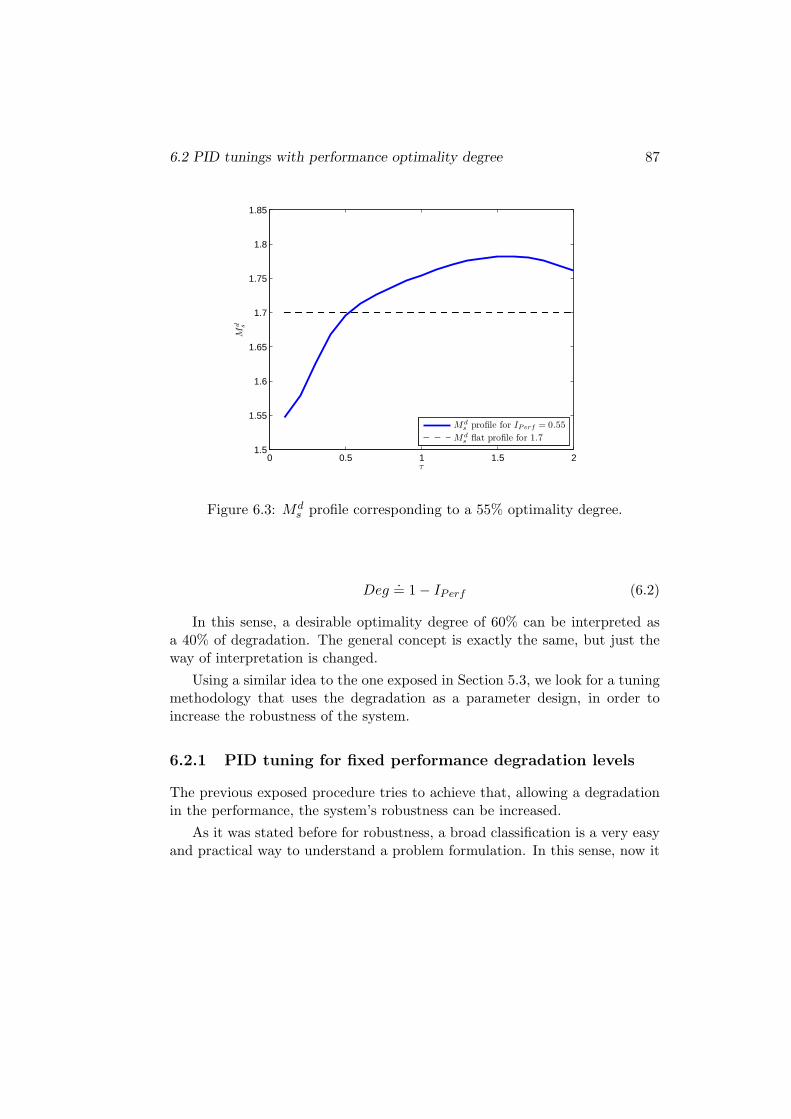
6.2 PID tunings with performance optimality degree 87
0 0.5 1 1.5 21.5
1.55
1.6
1.65
1.7
1.75
1.8
1.85
τ
Md s
Mds profile for IPerf = 0.55
Mds flat profile for 1.7
Figure 6.3: Mds profile corresponding to a 55% optimality degree.
Deg.= 1 − IPerf (6.2)
In this sense, a desirable optimality degree of 60% can be interpreted asa 40% of degradation. The general concept is exactly the same, but just theway of interpretation is changed.
Using a similar idea to the one exposed in Section 5.3, we look for a tuningmethodology that uses the degradation as a parameter design, in order toincrease the robustness of the system.
6.2.1 PID tuning for fixed performance degradation levels
The previous exposed procedure tries to achieve that, allowing a degradationin the performance, the system’s robustness can be increased.
As it was stated before for robustness, a broad classification is a very easyand practical way to understand a problem formulation. In this sense, now it

88 Optimality based PID control design
will be used the degradation of the system performance, Deg as a parameterto establish the levels.
To fix these degradation levels, we see information provided in Fig. 6.2.Here, the aim is to obtain profiles of Md
s for the range of τ ∈ [0.1, 2.0]. There-fore, the selected optimality degree level must intersect each one of the curvescorresponding to each one of the plants.
Fulfilling the above, to get a degree of optimality higher than 75%, therange of considered robustness should be extended to values greater thanMd
s = 2.0, but this value is the minimum acceptable robustness and for that,this option is not studied. From the other side, to have an optimality de-gree lower than 45% the robustness values must be minor than Md
s = 1.4,that is considered as a high robustness level, therefore decrease the degree ofoptimality to less than 45% (meaning a degradation more than 55%), is notjustified.
Then, the range of application was established as Deg ∈ [0.25, 0.55] andtherefore the classification as,
• Low degradation - Deg = 0.25
• Medium-low degradation - Deg = 0.35
• Medium-high degradation - Deg = 0.45
• High degradation - Deg = 0.55
As it was said above, for each stated degradation level and each τ , it isfound the corresponding Md
s . Then, the set of robustness values determinesthe Md
s profile, that is used in the proposed generic tuning (5.7) and (5.9),of section 5.3.2, to determine sets for each parameter of the PID controller,Kp, Ti and Td. Therefore, with all the parameters sets, the tuning rule can beformulated (by fitting).
Once again, following a similar idea to that described for the Mds case, the
aim is to provide a simple tuning and for that, we take advantage of the goodfitting that equations (5.7) provide. So, the sets for each PID parameter andfor each degradation level, are approximated to fit the corresponding equationsform.
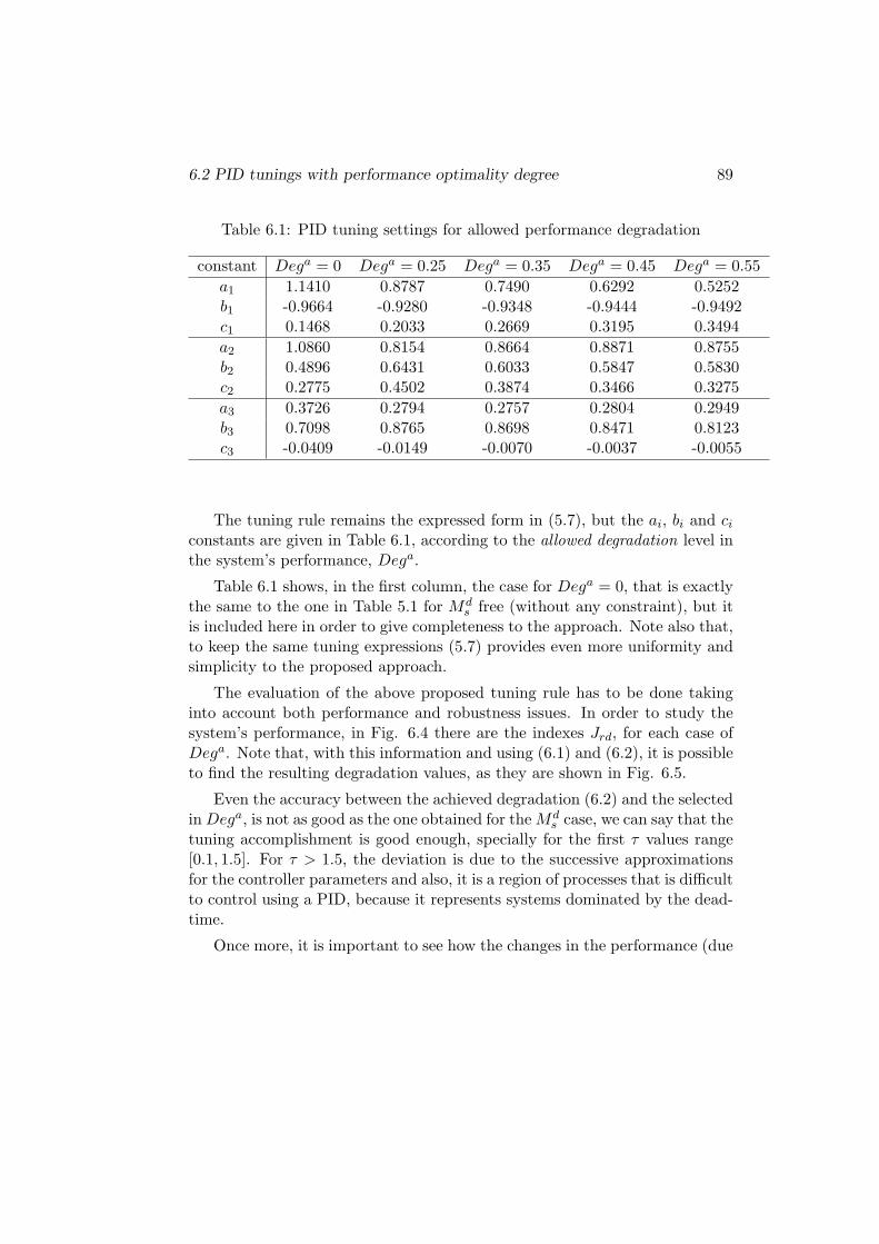
6.2 PID tunings with performance optimality degree 89
Table 6.1: PID tuning settings for allowed performance degradation
constant Dega = 0 Dega = 0.25 Dega = 0.35 Dega = 0.45 Dega = 0.55
a1 1.1410 0.8787 0.7490 0.6292 0.5252b1 -0.9664 -0.9280 -0.9348 -0.9444 -0.9492c1 0.1468 0.2033 0.2669 0.3195 0.3494
a2 1.0860 0.8154 0.8664 0.8871 0.8755b2 0.4896 0.6431 0.6033 0.5847 0.5830c2 0.2775 0.4502 0.3874 0.3466 0.3275
a3 0.3726 0.2794 0.2757 0.2804 0.2949b3 0.7098 0.8765 0.8698 0.8471 0.8123c3 -0.0409 -0.0149 -0.0070 -0.0037 -0.0055
The tuning rule remains the expressed form in (5.7), but the ai, bi and ci
constants are given in Table 6.1, according to the allowed degradation level inthe system’s performance, Dega.
Table 6.1 shows, in the first column, the case for Dega = 0, that is exactlythe same to the one in Table 5.1 for Md
s free (without any constraint), but itis included here in order to give completeness to the approach. Note also that,to keep the same tuning expressions (5.7) provides even more uniformity andsimplicity to the proposed approach.
The evaluation of the above proposed tuning rule has to be done takinginto account both performance and robustness issues. In order to study thesystem’s performance, in Fig. 6.4 there are the indexes Jrd, for each case ofDega. Note that, with this information and using (6.1) and (6.2), it is possibleto find the resulting degradation values, as they are shown in Fig. 6.5.
Even the accuracy between the achieved degradation (6.2) and the selectedin Dega, is not as good as the one obtained for the Md
s case, we can say that thetuning accomplishment is good enough, specially for the first τ values range[0.1, 1.5]. For τ > 1.5, the deviation is due to the successive approximationsfor the controller parameters and also, it is a region of processes that is difficultto control using a PID, because it represents systems dominated by the dead-time.
Once more, it is important to see how the changes in the performance (due

90 Optimality based PID control design
0 0.5 1 1.5 20.05
0.1
0.15
0.2
0.25
0.3
0.35
0.4
0.45
0.5
0.55
L/T
Jrd
Dega = 0.25Dega = 0.35Dega = 0.45Dega = 0.55
Figure 6.4: Combined index Jrd for each degradation level tuning.
to the imposed degradation), affects the achieved robustness for the system.Fig. 6.6 shows this evaluation, where the optimality decreases (i.e. degrada-tion increases), the robustness of the system grows up. This is an importantaspect because these Ms values represent the profile that should be accom-plished in order to achieve the fixed degradation (meaning a certain degree ofoptimality).
It can be seen, all results are in agreement regarding to the well knownperformance/robustness ratio.
6.2.2 PID tuning for an arbitrary performance degradation
Analogously to the tuning presented in Section 5.3.2, for arbitrary values ofMd
s , we want to give here a formulation that allow us to specify any value forthe allowed degradation. Because the approach is based on the informationprovided by the fixed degradation levels, the range of validity is within Dega ∈[0.25, 0.55].

6.2 PID tunings with performance optimality degree 91
0 0.5 1 1.5 20.2
0.25
0.3
0.35
0.4
0.45
0.5
0.55
0.6
0.65
L/T
Deg
Dega = 0.25Dega = 0.35Dega = 0.45Dega = 0.55
Figure 6.5: Accomplishment of the fixed degradation level tuning.
It is important to emphasize that, this extension is just possible becausethe simplicity and the homogeneity of the PID tuning parameters (5.7), thatremains the same expression for each one of the fixed degradation levels.
Once again, the aim is to provide a generic formulation in order to givecompleteness, as much as possible. Therefore, because each controller param-eter has the same form, we look for a general equation as,
pi(τ, Dega) = ai(Dega)τ bi(Dega) + ci(Dega) (6.3)
where i = 1, 2, 3 indicates the corresponding controller’s parameter, p, andconstants are expressed as functions of Dega. Then, from Table 6.1, theconstants ai, bi and ci with their respective Dega value, are fitted to a secondorder polynomial as

92 Optimality based PID control design
0 0.5 1 1.5 21.4
1.5
1.6
1.7
1.8
1.9
2
L/T
Ms
Dega = 0.25Dega = 0.35Dega = 0.45Dega = 0.55
Figure 6.6: Achieved robustness Ms for each degradation level tuning.
a1 = 0.6425(Dega)2 − 1.6940(Dega) + 1.2620
b1 = 0.0500(Dega)2 − 0.1132(Dega) − 0.9024
c1 = −0.8425(Dega)2 + 1.1650(Dega) − 0.0359
a2 = −1.5650(Dega)2 + 1.4530(Dega) + 0.5499
b2 = 0.9525(Dega)2 − 0.9609(Dega) + 0.8236 (6.4)
c2 = 1.0930(Dega)2 − 1.2830(Dega) + 0.7026
a3 = 0.4550(Dega)2 − 0.3128(Dega) + 0.3292
b3 = −0.7025(Dega)2 + 0.3467(Dega) + 0.8339
c3 = −0.2425(Dega)2 + 0.2255(Dega) − 0.0561
Specifically, parameters (5.7) jointly with the resulting constants (6.4),provide the PID controller tuning that choosing an arbitrary degradation valuefor the system performance, increases the robustness, as much as possible, forthe prescribed degree of optimality.

6.2 PID tunings with performance optimality degree 93
Table 6.2: Particular process - PID controller parameters for P8 (σ = 0.50)Tuning Dega Kp Ti Td
0.25 1.723 1.257 0.189Proposed 0.35 1.568 1.240 0.197(levels) 0.45 1.418 1.216 0.207
0.55 1.269 1.182 0.221
κ − τ (Mds = 2.0) - 1.719 1.151 0.285
Proposed Degκ−τ 1.529 1.234 0.199(generic)
6.2.3 Evaluation example
In order to evaluate the proposal, we take again advantage of system (5.11),P8(s), with σ = 0.50, shown in section 5.4.2 and also in this chapter, as aMotivation example.
From the FOPDT model and using tuning (5.7) for each fixed degrada-tion level in Table 6.1, the PID parameters can be obtained. Moreover, theproposed generic tuning (6.4), for arbitrary values of allowed degradation iscompared (setting the same degradation value), with the Kappa-Tau (κ − τ)(Astrom and Hagglund, 1995) for the Ms = 2.0 case. Tunings are shown inTable 6.2.
Comparisons with other tunings like AMIGO, Kappa-Tau for Ms = 1.4 orTavakoli, are not included because, as it can be seen in Fig. 6.1, the optimalitydegree values that they provide are outside the validity range of the proposedtuning, IPerf ∈ [0.45, 0.75] or seen from the allowed degradation point of view,Dega ∈ [0.25, 0.55].
Table 6.3 gives the performance and robustness values provided by eachtuning. Also, in Fig. 6.7 the control system’s and controller’s output areshown for each allowed degradation level, whereas in Fig. 6.8, it is possible tosee the comparison between the κ − τ tuning and the proposed settings withthe specific value of degradation.
From the two approaches for the proposal, it can be concluded that thelevels version has a good accuracy with respect to the selected value for theallowed performance degradation, giving at the same time an increase in therobustness. Concerning to the proposed tuning for an arbitrary value of Dega,

94 Optimality based PID control design
Table 6.3: Particular process P8 (σ = 0.50) - Controller evaluationTuning Dega Degr M r
s Jr Jd Jrd
0.25 0.2508 1.9780 1.4229 0.7568 0.3024Proposed 0.35 0.3575 1.8217 1.4421 0.8208 0.3609(levels) 0.45 0.4657 1.6923 1.4755 0.8954 0.4392
0.55 0.5645 1.5800 1.5283 0.9871 0.5438
κ − τ (Mds = 2.0) - 0.3325 2.0626 1.4597 0.7366 0.3189
Proposed Degκ−τ 0.3379 1.8474 1.4378 0.8086 0.3491(generic)
0 5 10 15 20 25 3070
75
80
85
time
y(t)
(%)
0 5 10 15 20 25 3060
70
80
90
100
time
u(t)
(%)
Dega = 0.25Dega = 0.35Dega = 0.45Dega = 0.55
Figure 6.7: Particular process P8 - Proposed method (σ = 0.50).
from Table 6.3 it is possible to see that compared to κ−τ , the achieved perfor-

6.3 Summary 95
0 5 10 15 20 25 3070
75
80
85
time
y(t)
(%)
0 5 10 15 20 25 3060
70
80
90
100
time
u(t)
(%)
κ− τ −Mds = 2.0
Proposed (generic) - Dega = Degκ−τ
Figure 6.8: Particular process P8 - Control system responses (σ = 0.50).
mance is practically the same (because they have the same degradation value),however, in the proposed tuning the robustness is much better. So, conclud-ing, for same performance, the proposed tuning provides greater robustness,making it a better option to tune the controller.
6.3 Summary
The control system’s trade-off between performance and robustness, can bestudied from two points of view. First, as it was shown in Chapter 5, select-ing a desirable value for robustness and facing to the resulting performancedegradation.

96 Optimality based PID control design
In this chapter, we formulated the problem from the other side, selecting anallowed performance degradation in order to get a higher robustness, respectto the case with zero degradation. The proposal is presented for some degra-dation levels (qualitative classification), and also for generic specific values ofdegradation within the range 25%-55%.
Results are presented as autotuning formulae, maintaining the same sim-plicity shown before for other proposed PID tuning approaches. The exampleshows the accuracy and the benefits of the contribution.
Chapter 7
Balancedperformance/robustness PIDdesign
Approaches presented in chapters 5 and 6 show two different ways to face withthe trade-off problem between performance and robustness issues. First, it wasproposed a tuning method that choosing a desired robustness Md
s , providesthe best servo/regulation performance that can be achieved for the system. Inthe second case, the idea is to reduce the degree of optimality of the system’sperformance, in order to increase the robustness. So, the tuning proposes toselect a certain degradation for the performance, that at the same time givesthe largest robustness increase.
Both approaches provide good results from the point of view they wereformulated and, of course, they are different, but complementary. However, itis necessary to go beyond and look for an intermediate idea, that provides abalance between the degree of optimality and the robustness increase.
7.1 Robustness increase measure
From the above, index (6.1) provides an idea about the degree of optimality forthe system’s performance. Here, we need to state a similar concept but withthe aim to quantify the robustness increase. Then, we compare the achieved
97
98 Balanced performance/robustness PID design
robustness of the constrained case with respect to the unconstrained one, thatis the optimum in performance but with lower robustness.
Therefore, the following index is proposed
IRob.=
∣∣∣∣
Mos − MJrd
s
Mos
∣∣∣∣
(7.1)
where Mos represents the robustness value achieved by tuning (5.4) without
any constraint for Ms (first column of Table 5.1), and MJrds is the robustness
value for the cases where the robustness is constrained (i.e. increased). Then,(7.1) is a normalized index, where as much as it grows, the robustness increasewill be larger.
Once more, we want to take advantage of the generic tuning rule, presentedin section 5.3.2, in order to evaluate the robustness increase for the wholerange of family plants within τ ∈ [0.1, 2.0]. Then, for each τ and each valueMd
s ∈ [1.4, 2.0], it is possible to find the PID parameters and obtain index(7.1). This procedure is analogous to the presented in the previous chapterfor IPerf index.
Fig. 7.1 shows the IRob variation, as a function of Mds , for some cases of the
normalized dead-time, τ . Each line represents the relative robustness increasefor a particular process (value of τ).
Note that in Fig. 7.1, we could define a certain value (level), for the robust-ness increase and with the intersection points, determine a suitable robustnessprofile (analogous to the procedure for IPerf in section 6.1). However, thisidea has the same objective to the tuning presented in chapter 5, that is toincrease the robustness of the system and provide at the same time, the bestservo/regulation performance. Here, as we stated before, the aim is to lookfor a balanced tuning.
7.2 Robustness/Performance balance
Taking into account that indexes (6.1) and (7.1) are both normalized into therange [0, 1], therefore having the same scale, if we put the information of Fig.6.2 and Fig. 7.1 all together, the intersection points for each pair of curves,can be interpreted as equilibrium points. These, represent when the degree ofoptimality is consistent to the robustness increase, and vice-versa.

7.3 Balanced PID tuning 99
1.4 1.5 1.6 1.7 1.8 1.9 20
0.1
0.2
0.3
0.4
0.5
0.6
0.7
Mds
I Rob
τ = 0.1τ = 0.3τ = 0.5τ = 0.7τ = 0.9τ = 1.1τ = 1.3τ = 1.5τ = 1.7τ = 1.9
Figure 7.1: Variation of the index IRob.
In Fig. 7.2, there are just few cases for the model normalized dead-timesτ , where it is possible to see the consideration exposed before.
With the intersection points between the corresponding pairs of curves, wecan determine the suitable set of desired robustness, that provides the best bal-ance between performance optimality degree and robustness increase. This setof Md
s (τ) determines the robustness profile for the best robustness/performancecompromise, for all the τ range. See Fig. 7.3.
7.3 Balanced PID tuning
As it has been explained before, with information provided by indexes IPerf
and IRob, it is possible to obtain the corresponding Mds value, that achieves the
best compromise between the loss of the optimality degree and the robustnessincrease.
The set of desired robustness values for all the plants within τ ∈ [0.1, 2.0],

100 Balanced performance/robustness PID design
1.4 1.45 1.5 1.55 1.6 1.65 1.70.1
0.2
0.3
0.4
0.5
0.6
0.7
0.8
Mds
I Perf,I
Rob
τ = 0.1τ = 0.5τ = 1.0τ = 1.5τ = 2.0
Figure 7.2: IPerf and IRob variation for some values of τ .
is a Mds profile that, as before, can be used in tuning (5.7) and (5.9), in order
to get the PID controller parameters.
Then, following the same aim to propose a simple and homogeneous tuning,the set for each parameter is fitted to the general tuning expressions (5.7).Therefore,
KpK = 0.6776τ−0.8630 + 0.1162
Ti
T= 0.9950τ0.4016 + 0.1564 (7.2)
Td
T= 0.2998τ0.9760 + 0.0110
Tuning (7.2) is the one that provides the best compromise/balance betweenthe robustness increase and the resulting loss of optimality degree for the sys-tem’s performance. It is important to note that also, because this performance

7.4 Tuning evaluation 101
0 0.5 1 1.5 21.44
1.46
1.48
1.5
1.52
1.54
1.56
1.58
1.6
L/T
Md s
Figure 7.3: Mds profile for the best robustness/performance balance.
index formulation, the trade-off problem between servo and regulation controloperation modes, is included.
7.4 Tuning evaluation
In this section, the intention is to evaluate the performance and robustnessfeatures for the proposed balanced tuning. Also, it is desirable to establish amore precise quantification of the balance concept, stated before. Therefore,we define the following index,
IB.=
∫ τf
τo
|IPerf (τ) − IRob(τ)|dτ (7.3)
where the idea is to measure the difference between the robustness increase andthe degree of optimality, for the whole range of plants τ ∈ [0.1, 2.0]. Note that,when the index (7.3) is low, it means a good balance between the robustness

102 Balanced performance/robustness PID design
increase and the corresponding price for performance optimality. A high valueof IB indicates a lack of balance for the studied indexes.
In Fig. 7.4, there are the robustness and servo/regulation performanceevaluation for the proposed balanced tuning and compared with the uncon-strained case, equivalent to Md
s free and/or Dega = 0. There, it can be seenthe robustness increase, as well as the consequent loss of degree of optimalityfor the system’s performance.
0 0.5 1 1.5 21.4
1.6
1.8
2
2.2
2.4
2.6
2.8
3
L/T
Ms
Tuning for Md
s − free / Dega = 0Proposed balanced tuning
0 0.5 1 1.5 20
0.2
0.4
0.6
0.8
1
1.2
1.4
L/T
Jrd
Tuning for Md
s − free / Dega = 0Proposed balanced tuning
Figure 7.4: Robustness and performance values for proposed tuning.
In addition, Fig. 7.5 shows IPerf and IRob indexes for the proposed bal-anced tuning (7.2), where the similarity between the values indicates that, forthe whole τ range, the robustness increase is equivalent to the loss of perfor-mance’s optimality, therefore having a balance. It means a “fair price betweenwhat is paid and what is got”.
Table 7.1 shows the balanced index IB, for each one of the proposed tuningrules and also compared with AMIGO and Kappa-Tau methods.
It is possible to see that, apart from the case for proposed balanced tuningthat has obviously the best IB index, tuning with Md
s = 1.6 is the one thatprovides lower value for the balanced index (7.3). This has a lot of sensebecause, if we look in Fig. 7.3, the robustness profile in almost the cases arewithin the range [1.5, 1.6].
Moreover, AMIGO tuning has a better IB index than its counterpart for

7.5 Comparison example 103
0 0.5 1 1.5 20.2
0.25
0.3
0.35
0.4
0.45
0.5
I Perf,I
Rob
L/T
IP erf for proposed balanced tuningIRob for proposed balanced tuning
Figure 7.5: IPerf and IRob indexes for the proposed balanced tuning.
proposed Mds = 1.4. However, this is again for the previously exposed non-
accomplishment of the specified robustness for the AMIGO method. If weuse the generic tuning for Md
s , in order to reproduce the robustness profile forAMIGO (Md
s = MAMIGOs ), it is possible to see in Table 7.1, that this resulting
tuning provides a better robustness/performance balance.
7.5 Comparison example
We will use again system (5.11), P8(s), with σ = 0.50, in order to evaluate theproposed balanced tuning.
From the FOPDT model information and applying the proposed balancedtuning (7.2), it is possible to obtain the PID parameters as: Kp = 1.244,Ti = 1.174 and Td = 0.224. Here, the idea is to evaluate the robustnessand performance provided for the balanced tuning and also to compare with:AMIGO and proposed generic tuning for Md
s = MAMIGOs and Kappa-Tau

104 Balanced performance/robustness PID design
Table 7.1: Balanced index 7.3 for different tuning rulesTuning Criteria design IB
AMIGO Mds = 1.4 0.2900
κ − τ Mds = 1.4 2.1373
κ − τ Mds = 2.0 3.6303
Mds = 1.4 0.3163
Mds = 1.6 0.1416
Proposed Mds = 1.8 0.7011
Mds = 2.0 1.3228
Mds = MAMIGO
s 0.2512
Dega = 0.25 1.0513Proposed Dega = 0.35 0.7987
Dega = 0.45 0.5482Dega = 0.55 0.2956
Proposed Balanced-IB 0.0070
Table 7.2: Particular process P8 (σ = 0.50) - Controller tuning evaluationTuning Criteria design IPerf IRob |IPerf − IRob|
AMIGO Mds = 1.4 0.2913 0.4651 0.1738
Proposed Mds = MAMIGO
s 0.3186 0.4650 0.1464
κ − τ Mds = 2.0 0.6675 0.2359 0.4316
Proposed Dega = Degκ−τ 0.6621 0.3156 0.3465
Proposed Balanced-IB 0.4202 0.4211 0.0009
(Ms = 2.0) and the proposed tuning for an arbitrary degradation value ofDega = Degκ−τ . Controller’s parameters for these last tuning methods canbe found in Tables 5.4 and 6.2.
In Table 7.2, the indexes (6.1) and (7.1) are shown, as well as the corre-sponding difference |IPerf−IRob|, that indicates the system robustness/performancebalance. Just to remember, index IPerf indicates the degree of optimality forthe system, so it is desired high values near to one. Then, for the system’srobustness increase IRob, it must be as large as possible.
The comparison shown in Table 7.2 provides that, as expected, AMIGOand proposed generic tuning for Md
s = MAMIGOs have an equal IRob value,

7.6 Summary 105
because their robustness is the same. However, the proposed Mds tuning has
a higher performance optimality degree than AMIGO, therefore achieving abetter balance (less |IPerf − IRob| value).
For the Kappa-Tau and proposed tuning with Dega = Degκ−τ , we havean analogous result because, for similar IPerf index values, the robustnessincrease achieved by proposed tuning for arbitrary Dega values, is higher thanthe one for κ− τ method and therefore, the balance is better for the proposal.
Finally, the last row of Table 7.2 gives the evaluation for the proposed bal-anced tuning (7.2), that has obviously the best balance calculation, meaninga similar values for IPerf and IRob. For this system, it is possible to see thatthe best balance can be obtained when the performance degree of optimalityand the robustness increase, are values around the 40%.
In Fig. 7.6, there are the system’s and controller’s outputs for three casesof the proposed tuning. It is possible to see that, responses for the balancedtuning are between the ones that provide the best values for IPerf and IRob
indexes.
7.6 Summary
In this chapter a new PID tuning methodology is proposed, with the aim toachieve the best possible balance between robustness and performance issues.The problem was faced using the results presented in chapters 5 and 6.
The proposal is presented as an autotuning rule, where just the FOPDTmodel information is needed to calculate the PID controller parameters. Thisproposed balanced tuning looks for the best compromise between the robust-ness increase and the consequent reduction in the performance optimality forthe system.
An important aspect of the proposed balanced tuning is that, it remainsthe same expression for the controller’s parameters than the previous proposedones for Md
s and Dega, providing a complete and homogeneous set of optionsto tune the PID.
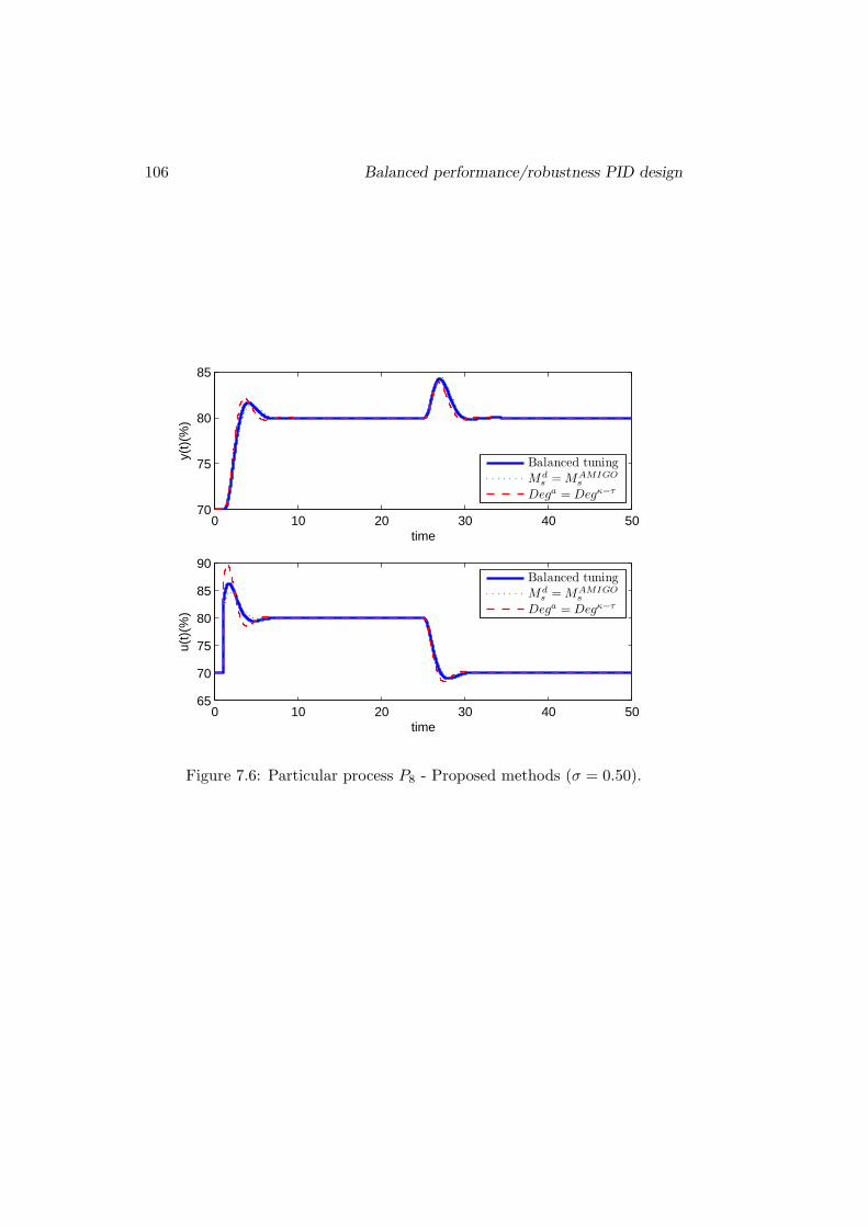
106 Balanced performance/robustness PID design
0 10 20 30 40 5070
75
80
85
time
y(t)
(%)
Balanced tuningMd
s = MAMIGOs
Dega = Degκ−τ
0 10 20 30 40 5065
70
75
80
85
90
time
u(t)
(%)
Balanced tuningMd
s = MAMIGOs
Dega = Degκ−τ
Figure 7.6: Particular process P8 - Proposed methods (σ = 0.50).

Part III
Concluding remarks
107


Chapter 8
Conclusions and future work
This thesis faces to various and very important aspects of PID control, suchas performance and robustness. The main objective is to provide answers tothe very well known trade-off problems, between performance for servo andregulation operation and between performance and robustness features.
From the above, the proposed tuning methodologies take into account theseconsiderations, in order to improve the general behavior of the control system.
This chapter concludes the work presented in this thesis and gives someclues for future work and research.
8.1 Conclusions and contributions
New autotuning methods for PID controllers have been presented. Thesemethods use the information provided by a FOPDT model of the process, toobtain the controller’s parameters. The design looks for the essential require-ments of any control system as combined servo/regulation performance androbustness with respect to model uncertainties. The formulation of the designproblems were divided in two approaches (corresponding to the two parts ofthis document).
Part I: Combined servo/regulation operation for PID controllers
It is presented a general procedure to find an intermediate tuning for servo/regulation control operation, in order to reduce the performance degradation
109

110 Conclusions and future work
when the system operates in a different way that it was tuned for. Thisapproach is stated in terms of the extreme optimal tunings for each operationmode and weighting factors can be used, as a qualitative specification, todeclare a preference between both operation modes.
The resulting intermediate tuning provides lower performance than the op-timum settings when the tuning and the operation modes are equal. However,in general terms, if we take into account the whole system operation (servoand regulation), it is possible to achieve the highest performance when theproposed intermediate tuning is used.
In addition of the above idea, the general procedure was extended to unsta-ble an integrating processes showing that for this application, the proposal iseven better because the expected performance degradation is very high, whenthe tuning and operation modes are different. Therefore, the improvementthat can be achieved using the intermediate tuning, results in a good optionto obtain the PID controller parameters.
Part II: Robustness and performance trade-off for PID controllers
The proposed approaches include the consideration of robustness, in an explicitway into the design stage. First, it was presented a tuning rule that selecting adesired robustness Md
s , provides the best servo/regulation performance (5.4),that can be achieved for the system. The accomplishment of the claimedrobustness was verified, obtaining almost negligible deviation values, thereforethe PID controller gives a good performance with also a precise and certainrobustness degree.
In the second case, it is proposed an approach that, even different, iscomplementary to the previous one. The idea is to allow some reduction inthe optimality degree of the system’s performance, in order to achieve thelargest increase in the robustness. Some evaluations show the good results forthe proposed tunings compared with other well-known PID methods.
Finally, it was desirable to look for an intermediate approach that providesa balance between the degree of optimality and the robustness increase and inthis sense, a well-balanced PID tuning was presented (7.2).
A very important aspect of this second part is that, all PID tuning methodswere parametrized using the same form for the equations of controller’s pa-rameters (5.7). This allows to maintain simple and homogeneous expressions

8.2 Future work and research 111
that can be implemented easily.
8.2 Future work and research
Some ideas to extend or to explore new opportunities from this research study,can be followed in future works.
• Process model information. The proposed tunings were based onthe information provided by a FOPDT model. To develop the sameprocedure for Second-Order-Plus-Dead-Time (SOPDT) models, couldimprove the whole system’s behavior. Moreover, although in the firstpart the results were presented for unstable and integrating processescases, could be interesting to follow the proposed ideas in the secondpart for these kind of systems and even more, to study the non-minimumphase systems (inverse response).
• PID controller structure. Taking into account the little-known offractional PID controllers, could be very interesting to explore the servo/regulation dynamics, as well as the robustness, in this kind of PID. Forits novelty, it is a point that can receive much attention.
Another approach is to obtain the four parameters of a 2-DoF PID con-troller just with a single optimization of index (5.4). This could improvethe actual and well-known procedure of two stages (first one for reg-ulation and then for servo). A systematic way to determine when aPID should be of one or two degrees of freedom (1-DoF/2-DoF) is verywelcome.
• Control configuration. Considering that, usually control systems op-erate in regulation mode and set-point changes can be predicted, theformulation of an adaptive re-tuning design between servo/regulationtuning modes could be investigated. Also, the researched topic could bestudied for multivariable systems, specifically for TITO processes, con-sidering that it is a system that follows a set-point but has continuousdisturbances, produced by the interaction effects between the control-loops.

112 Conclusions and future work
• Real implementation. The proposed PID controller tunings imple-mented by simulation in this work, can be tested and performed in realplants.

References
Alfaro, V. M. (2006). Low-order models identification from process reactioncurve. Ciencia y Tecnologıa (Costa Rica) 24(2), 197–216. (in Spanish).
Alfaro, V. M., R. Vilanova and O. Arrieta (2009). A Single-Parameter RobustTuning Approach for Two-Degree-of-Freedom PID Controllers. In: Eu-ropean Control Conference (ECC09). pp. 1788–1793. Budapest-Hungary.
Ali, A. and S. Majhi (2010). PID controller tuning for integrating processes.ISA Transactions 49(1), 70–78.
Araki, M. and H. Taguchi (1998). Two-Degree-of-Freedom PID controller.Systems, Control and Information 42, 18–25.
Araki, M. and H. Taguchi (2003). Two-Degree-of-Freedom PID Controllers.International Journal of Control, Automation, and Systems 1, 401–411.
Arrieta, O. (2007). PID Control: A tradeoff tuning for Servo/Regulation oper-ation. Master’s thesis. Dept.Telecomunicacio i d’Enginyeria de Sistemes,Universitat Autonoma de Barcelona, Barcelona, Spain.
Arrieta, O., A. Ibeas and R. Vilanova (2009a). Stability Analysis for the Inter-mediate Servo/Regulation PID Tuning. In: 14th IEEE International Con-ference on Emerging Technologies and Factory Automation (ETFA09),September 22-26, Mallorca-Spain.
Arrieta, O., A. Visioli and R. Vilanova (2009b). Improved PID Autotuning forbalanced control operation. In: 14th IEEE International Conference onEmerging Technologies and Factory Automation (ETFA09), September22-26, Mallorca-Spain.
113

114 REFERENCES
Arrieta, O., A. Visioli and R. Vilanova (2010). PID autotuning forweighted servo/regulation control operation. Journal of Process Control20(4), 472–480.
Arrieta, O. and R. Vilanova (2007a). Performance degradation analysis of Op-timal PID settings and Servo/Regulation tradeoff tuning. In: Conferenceon Systems and Control (CSC07), May 16-18, Marrakech-Morocco.
Arrieta, O. and R. Vilanova (2007b). PID Autotuning settings for balancedServo/Regulation operation. In: 15th IEEE Mediterranean Conferenceon Control and Automation (MED07), June 27-29, Athens-Greece.
Arrieta, O. and R. Vilanova (2007c). Servo/Regulation tradeoff tuning ofPID controllers with a robustness consideration. In: 46th IEEE Confer-ence on Decision and Control (CDC07), December 12-14, New Orleans,Louisiana-USA.
Arrieta, O. and R. Vilanova (2007d). Stability margins characterizationof a combined Servo/Regulation tuning for PID controllers. In: 12thIEEE Conference on Emerging Technologies and Factory Automation(ETFA07), September 25-28, Patras-Greece.
Arrieta, O. and R. Vilanova (2010). Performance degradation analysis ofcontroller tuning modes: Application to an optimal PID tuning. In-ternational Journal of Innovative Computing, Information and Control6(10), 4719–4729.
Arrieta, O., R. Vilanova, V. M. Alfaro and R. Moreno (2008). Considerationson PID Controller Operation: Application to a Continuous Stirred TankReactor. In: 13th IEEE International Conference on Emerging Tech-nologies and Factory Automation (ETFA08), September 15-18, Hamburg-Germany.
Astrom, K.J. and T. Hagglund (1984). Automatic tuning of simple regula-tors with with specifications on phase and amplitude margin. Automatica20, 645–651.
Astrom, K.J. and T. Hagglund (1995). PID Controllers: Theory, Design, andTuning. Instrument of Society of America.
REFERENCES 115
Astrom, K.J. and T. Hagglund (2000). Benchmark Systems for PID control.In: IFAC Digital Control: Past, Present and Future of PID Control.Terrassa, Spain.
Astrom, K.J. and T. Hagglund (2001). The future of PID control. ControlEngineering Practice 9, 1163–1175.
Astrom, K.J. and T. Hagglund (2004). Revisiting the Ziegler-Nichols stepresponse method for PID control. Journal of Process Control 14, 635–650.
Astrom, K.J. and T. Hagglund (2006). Advanced PID Control. ISA - TheInstrumentation, Systems, and Automation Society.
Babb, M. (1990). Pneumatic Instruments Gave Birth to Automatic Control.Control Engineering 37(12), 20–22.
Bascetta, L. and A. Leva (2008). FIR based causal design of 2-DOF controllersfor optimal set point tracking. Journal of Process Control 18, 465–478.
Bennett, S. (2000). The Past of PID Controllers. In: IFAC Digital Control:Past, Present and Future of PID Control. Terrassa, Spain.
Chen, D. and D.E. Seborg (2002). PI/PID controller design based on directsynthesis and disturbance rejection. Industrial Engineering & ChemistryResearch. 41(19), 4807–4822.
Chidambaram, M. and R. Padma Sree (2003). A simple method of tuningPID controllers for integrator/dead-time processes. Computers & Chem-ical Engineering 27(2), 211–215.
Cohen, G. H. and G. A. Coon (1953). Theoretical Considerations of RetardedControl. ASME Transactions 75, 827–834.
Fung, H.W., Q.G. Wang and T.H. Lee (1998). PI Tuning in terms of gain andphase margins. Automatica 34, 1145–1149.
Ge, M., M. Chiu and Q. Wang (2002). Robust PID controller design via lmiapproach. Journal of Process Control 12, 3–13.
Ho, M.T. and C.Y. Lin (2003). PID controller design for robust performance.IEEE Trans. Automat. Contr. 48(8), 1404–1409.
116 REFERENCES
Ho, W. K., C. C. Hang and L. S. Cao (1995). Tuning PID Controllers Basedon Gain and Phase Margin Specifications. Automatica 31(3), 497–502.
Ho, W. K., K. L. Lim, C. C. Hang and L. Y. Ni (1999). Getting more phasemargin and performance out of PID controllers. Automatica 35, 1579–1585.
Ingimundarson, A., T. Hagglund and K. J. Astrom ((n.d.)). Criteria for desingof PID controllers. Technical report. ESAII, Universitat Politecnica deCatalunya.
Khalil, Hassa K. (2002). Nonlinear Systems. Prentice Hall, Inc.
Kim, Don Hwa (2004). The Comparison of Characteristics of 2-DOF PIDControllers and Intelligent Tuning for a Gas Turbine Generating Plant.Springer Berlin / Heidelberg, Lecture Notes in Computer Science.
Kim, Dong Hwa (2002). Tuning of 2-DOF PID controller by immune algo-rithm. In: Congress on Evolutionary Computation (CEC’02), May 12-17,Honolulu, HI-USA. pp. 675–680.
Kravaris, C. and P. Daoutidis (1990). Nonlinear state feedback control of sec-ond order nonminimum-phase nonlinear systems. Computers Chem. Eng.14(4-5), 439–449.
Kristiansson, B. and B. Lennartson (2006). Evaluation and simple tuning ofPID controllers with high-frequency robustness. Journal of Process Con-trol 16, 91–102.
Lee, Yongho, Jeongseok Lee and Sunwon Park (2000). PID controller tuningfor integrating and unstable processes with time delay. Chemical Engi-neering Science 55(17), 3481–3493.
Leva, A. and L. Bascetta (2007). Set point tracking optimisation by causalnonparametric modelling. Automatica 11, 1984–1991.
Lopez, A. M., J. A. Miller, C. L. Smith and P. W. Murrill (1967). Tuning con-trollers with Error-Integral criteria. Instrumentation Technology 14, 57–62.

REFERENCES 117
Martin, J., C. L Smith and A. B. Corripio (1975). Controller Tuning fromSimple Process Models. Instrumentation Technology 22(12), 39–44.
Mitchell, M. (1998). An Introduction to Genetic Algorithms. MIT Press, USA.
O’Dwyer, A. (2003). Handbook of PI and PID Controller Tuning Rules. Im-perial College Press, London, UK.
Panda, Rames C. (2009). Synthesis of PID controller for unstable and inte-grating processes. Chemical Engineering Science 64(12), 2807–2816.
Pedret, C., R. Vilanova, R. Moreno and I. Serra (2002). A refinement pro-cedure for pid controller tuning. Computers & Chemical Engineering26, 903–908.
Rivera, D. E., M. Morari and S. Skogestad (1986). Internal model control 4.pid controller design. Ind. Eng. Chem. Res. 25, 252–265.
Rovira, A., P. W. Murrill and C. L. Smith (1969). Tuning controllers forsetpoint changes. Instrumentation & Control Systems 42, 67–69.
Silva, G.J., A. Datta and S.P. Battacharayya (2002). New Results on thesynthesis of PID controllers. IEEE Trans. Automat. Contr. 47(2), 241–252.
Skogestad, S. (2003). Simple analytic rules for model reduction and PID con-troller tuning. Journal of Process Control 13, 291–309.
Sree, R. Padma and M. Chidambaram (2006). Control of Unstable Systems.Alpha Science International Ltd., UK.
Sree, R. Padma, M. N. Srinivas and M. Chidambaram (2004). A simple methodof tuning PID controllers for stable and unstable FOPTD systems. Com-puters & Chemical Engineering 28(11), 2201–2218.
Taguchi, H. and M. Araki (2000). Two-Degree-of-Freedom PID controllers- Their functions and optimal tuning. In: IFAC Digital Control: Past,Present and Future of PID Control. Terrassa, Spain.
Tan, W., J. Liu, T. Chen and H. J. Marquez (2006). Comparison of somewell-known PID tuning formulas. Computers & Chemical Engineering30, 1416–1423.
118 REFERENCES
Tavakoli, S., I. Griffin and P. J. Fleming (2005). Robust PI controller for loaddisturbance rejection and setpoint regulation. In: IEEE Conference onControl Applications. Toronto, Canada.
Toscano, R. (2005). A simple pi/pid controller design method via numericaloptimizatio approach. Journal of Process Control 15, 81–88.
Van de Vusse, J. G. (1964). Plug-flow type reactor versus tank reactor. Chem.Eng. Sci. 19, 964.
Vilanova, R. (2008). IMC based robust PID design: Tuning guidelines andautomatic tuning. Journal of Process Control.
Vilanova, R., V. M. Alfaro, O. Arrieta and C. Pedret (2010). Analysis ofthe claimed robustness for PI/PID robust tuning rules. In: 18th IEEEMediterranean Conference on Control and Automation (MED10), June23-25, Marrakech-Morocco.
Visioli, A. (2001). Optimal tuning of PID controllers for integral and unstableprocesses. IEE Proceedings - Control Theory Applications 148(2), 180–184.
Visioli, A. (2006). Practical PID Control. Springer Verlag Advances in Indus-trial Control Series.
Vivek, Sathe and M. Chidambaram (2005). An improved relay auto tuningof PID controllers for unstable FOPTD systems. Computers & ChemicalEngineering 29(10), 2060–2068.
Yaniv, O. and M. Nagurka (2004). Design of PID controllers satisfying gainmargin and sensitivity constrains on a set of plants. Automatica 40, 111–116.
Zhang, Jing-Gang, Zhi-Yuan Liu and Run Pei (2002). Two degree-of-freedomPID control with fuzzy logic compensation. In: First International con-ference on Machine Learning and Cybernetics, November 4-5, Beijing-China. pp. 1498–1501.
Zhuang, M. and D. Atherton (1993). Automatic tuning of optimum PID con-trollers. IEE Proceedings.Part D. 140(3), 216–224.

REFERENCES 119
Ziegler, J.G. and N.B. Nichols (1942). Optimum Settings for Automatic Con-trollers. ASME Transactions pp. 759–768.