Computational Physics Chapter 5 Numerical Solution of Linear System of Equations

Computational Physics

Chapter 5

Numerical Solution of Linear System of Equations

Prof. Kamal Al Saleh

Department of Physics

University of Jordan

Second Semester 2013/2014

[email protected]

5.1 Introduction

Linear system of equations are associated with many problems in science and engineer-

ing and many other applications.

5.2 Gaussian Elimination and Backward Substitution

Consider a general linear system of equations:

eq1 : a11 x1 + a12 x2 + a13 x3 + a14 x4 = b1 ;

eq2 : a21 x1 + a22 x2 + a23 x3 + a24 x4 = b2 ;

eq3 : a31 x1 + a32 x2 + a33 x3 + a34 x4 = b3 ;

eq4 : a41 x1 + a42 x2 + a43 x3 + a44 x4 = b4 ;

We use three operations to simplify the linear system given above:

1. Equation eqi can be multiplied by any nonzero constant l and the resulting equation

used in place of eqi. This operation is denoted as: Hl eqiL Ø HeqiL .

2. Equation eq j can be multiplied by any constant l , added to equation eqi, and the

resulting equation used in place of eqi. This operation is denoted as:

Heqi + l eq jL Ø HeqiL .

3. Equation eqi and eq j can be transposed in order. This operation is denoted by:

Chapter-5.nb 1

HeqiL¨ Heq jL.

By a sequence of the operations just given, a linear system can be transformed to a

more easily solved linear system with the same solution.

Example 1

Lets first consider the following example of a given system of equations to be solved

for x1, x2, x2, and x4 using the Gaussian elimination method. Given the equations as:

eq1 : x1 + x2 + ... .. + 3 x4 = 4 ;

eq2 : 2 x1 + x2 - x3 + x4 = 1 ;

eq3 : 3 x1 - x2 - x3 + 2 x4 = -3 ;

eq4 : -x1 + 2 x2 + 3 x3 - x4 = 4 ;

Mathematica Solution

Clear@"Global`∗"D

eq1 = x@1D + x@2D + 3 x@4D � 4;

eq2 = 2 x@1D + x@2D − x@3D + x@4D � 1;

eq3 = 3 x@1D − x@2D − x@3D + 2 x@4D � −3;

eq4 = −x@1D + 2 x@2D + 3 x@3D − x@4D � 4;

sol = Solve@8eq1, eq2, eq3, eq4<,

8x@1D, x@2D, x@3D, x@4D<D êê Flatten

sol2 = NSolve@8eq1, eq2, eq3, eq4<,

8x@1D, x@2D, x@3D, x@4D<D

x@4D = x@4D ê. sol;

Print@"x@4D = ", x@4DD

8x@1D → −1, x@2D → 2, x@3D → 0, x@4D → 1<

88x@1D → −1., x@2D → 2.,

x@3D → −1.29526×10−16

, x@4D → 1.<<

x@4D = 1

Chapter-5.nb 2

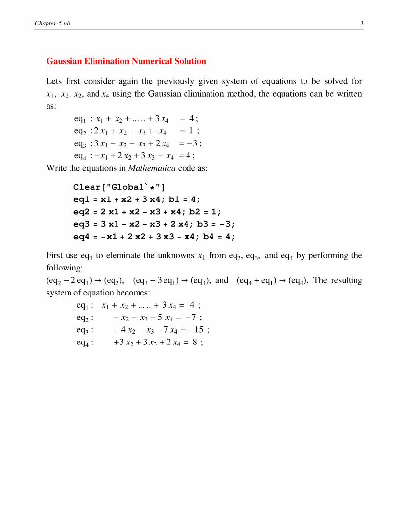
Gaussian Elimination Numerical Solution

Lets first consider again the previously given system of equations to be solved for

x1, x2, x2, and x4 using the Gaussian elimination method, the equations can be written

as:

eq1 : x1 + x2 + ... .. + 3 x4 = 4 ;

eq2 : 2 x1 + x2 - x3 + x4 = 1 ;

eq3 : 3 x1 - x2 - x3 + 2 x4 = -3 ;

eq4 : -x1 + 2 x2 + 3 x3 - x4 = 4 ;

Write the equations in Mathematica code as:

Clear@"Global`∗"D

eq1 = x1 + x2 + 3 x4; b1 = 4;

eq2 = 2 x1 + x2 − x3 + x4; b2 = 1;

eq3 = 3 x1 − x2 − x3 + 2 x4; b3 = −3;

eq4 = −x1 + 2 x2 + 3 x3 − x4; b4 = 4;

First use eq1 to eleminate the unknowns x1 from eq2, eq3, and eq4 by performing the

following:

Heq2 - 2 eq1L Ø Heq2L, Heq3 - 3 eq1L Ø Heq3L, and Heq4 + eq1L Ø Heq4L. The resulting

system of equation becomes:

eq1 : x1 + x2 + ... .. + 3 x4 = 4 ;

eq2 : - x2 - x3 - 5 x4 = -7 ;

eq3 : - 4 x2 - x3 - 7 x4 = -15 ;

eq4 : +3 x2 + 3 x3 + 2 x4 = 8 ;

Chapter-5.nb 3

8eq2 = Heq2 − 2 eq1L êê Expand,

b2 = Hb2 − 2 b1L, eq3 = Heq3 − 3 eq1L êê Expand,

b3 = b3 − 3 b1, eq4 = Heq4 + eq1L, b4 = b4 + b1<;

eq1 � b1

eq2 � b2

eq3 � b3

eq4 � b4

x1 + x2 + 3 x4 � 4

−x2 − x3 − 5 x4 � −7

−4 x2 − x3 − 7 x4 � −15

3 x2 + 3 x3 + 2 x4 � 8

In the new system of equations, eq2 is used to eliminate x2 from eq3 and eq4 , by

performing the following:

Heq3 - 4 eq2L Ø Heq3L, and Heq4 + 3 eq2L Ø Heq4L. The resulting system of equation

becomes:

eq1 : x1 + x2 + ... .. + 3 x4 = 4 ;

eq2 : - x2 - x3 - 5 x4 = -7 ;

eq3 : +3 x3 + 13 x4 = 13 ;

eq4 : -13 x4 = -13 ;

Chapter-5.nb 4

8eq3 = Heq3 − 4 eq2L êê Expand, b3 = Hb3 − 4 b2L,

eq4 = Heq4 + 3 eq2L êê Expand, b4 = b4 + 3 b2<;

eq1 � b1

eq2 � b2

eq3 � b3

eq4 � b4

x1 + x2 + 3 x4 � 4

−x2 − x3 − 5 x4 � −7

3 x3 + 13 x4 � 13

−13 x4 � −13

The new system of equations is now in triangular ( or reduced ) form and can be

solved for the unknowns by a backward-substitution process. Noting that eq4

implies x4 = 1, eq3 can be solved for x3 to give:

x3 =1ÅÅÅÅ3 H13 - 13 x4L = 1ÅÅÅÅ

3 H13 - 13L = 0.

Continuing to solve eq2 to give:

x2 = H7 - 5 x4 - x3L = H7 - 5 - 0L = 2.

and eq1 gives:

x1 = 4 - 3 x4 - x2 = 4 - 3 - 2 = -1.

The solution to the set of equations is: x1 = -1, x2 = 2, x3 = 0, and x4 = 1.

sol1 = Solve@eq1 � b1, x1D êê Flatten;




Chapter-5.nb 5

x1 = x1 ê. sol1; x2 = x2 ê. sol2;

x3 = x3 ê. sol3; x4 = x4 ê. sol4;

8x1, x2, x3, x4<

Print@"x1 = ", x1, " ; ", " x2 = ", x2,

" ; ", " x3 = ", x3, " ;", " x4 = ", x4D

8−1, 2, 0, 1<

x1 = −1 ; x2 = 2 ; x3 = 0 ; x4 = 1

When performing the calculations of this example we did not need to write out the full

equations at each step or to carry the variables x1, x2, x3, and x4 through the calcula-

tions, since they always remained in the same column. The only variation from system

to system occurred in the coefficients of the unknowns and in the values on the right-

side of the equations. For this reason, a linear system is often replaced by a matrix,

which contains all the information about the system that is necessary to determine its

solution, but in a compact form. That is to say: an n by m matrix is a rectangular array

of elements with n rows and m columns in which not only is the value of an element

important, but also its position in the array.

The General Matrix Notations

The notation for the näm (n by m) augmented matrix is a rectangular array of elements

with n rows and m columns in which not only is the value of an element important, but

also its position in the array. Consider the following general linear system of equations:

eq1 = a11 x1 + a12 x2 + a13 x3 == b1

eq2 = a21 x1 + a22 x2 + a23 x3 == b2

eq3 = a31 x1 + a32 x2 + a33 x3 == b3

these equations can be represented in matrix of the coefficient A, and a column matrix

of the constants b, expressed as:

A =

i

kjjjjjj

a11 a12 a13

a21 a22 a23

a31 a32 a33

y

{zzzzzz and b =

i

kjjjjjj

b1

b2

b3

y

{zzzzzz

Chapter-5.nb 6

or these two matrices can be combined in what so called the augmented matrix repre-

sented as:

@A, bD =i

kjjjjjj

a11 a12 a13 b1

a21 a22 a23 b2

a31 a32 a33 b3

y

{zzzzzz

In general an n by (n+1) matrix can be used to represent the following linear system of

equations:

a11 x1 + a12 x2 + ... ... + a1 n xn = b1 = a1,n+1

a21 x1 + a22 x2 + ... ....+a2 n xn = b2 = a2,n+1

a31 x1 + a32 x2 + ... ....+a3 n xn = b3 = a3,n+1

. . . .

. . . .

an,1 x1 + an,2 x2 + ... ....+an,n xn = bn = an,n+1

where the augmented matrix for these equations is represented as:

@A, bD = Aè=

i

k

jjjjjjjjjjjjjjjj

a11 a12 . . a1 n a1,n+1

a21 a22 . . a23 a2,n+1

. . . . . .

. . . . . .

an1 an2 . . an n an,n+1

y

{

zzzzzzzzzzzzzzzz

Provided that a11 ∫ 0, an reduction operation corresponding to Ieqi -ai,1ÅÅÅÅÅÅÅÅa1,1

eq1M Ø eqi

are performed for each row i = 2, 3, ... n to eliminate the coefficient of x1 in each of

these rows. In general, the reduction operation follow a sequential procedure as: for

i = j + 1, ... .., n and for j = 1, 2, ... n - 1 , provided that a j, j ∫ 0, perform the row

reduction operations I eqi -ai, jÅÅÅÅÅÅÅÅa j, j

eq j MØ eqi. The resulting matrix is :

Chapter-5.nb 7

Aè=

i

k

jjjjjjjjjjjjjjj

a11 a12 . . a1 n a1 n+1

0 a22 . . a23 a2 n+1

. . . . . .

. . . . . .

0 0 . . an n an n+1

y

{

zzzzzzzzzzzzzzz

This is called the upper triangular matrix U. The lower triangular matrix L has all zero

elements above

the major diagonal. This reduced matrix corresponds to following linear equations :

a11 x1 + a12 x2 + ... ... ... + a1,n = a1,n+1

a22 x2 + ... ... ... + a2,n = a2,n+1

... ... ... an, n = an,n+1

Solving the nth equation for xn we need the back substitution in the last n'th equation

thus:

xn =an,n+1ÅÅÅÅÅÅÅÅÅÅÅÅÅan n

Solving for the (n-1)st equation for xn-1 and using the calculated xn yields :

xn-1 =an-1,n+1-an-1,n xnÅÅÅÅÅÅÅÅÅÅÅÅÅÅÅÅÅÅÅÅÅÅÅÅÅÅÅÅÅÅÅÅÅÅ

an-1,n-1

and counting this process backward, we obtain for each i = n - 1, n - 2, ... .. 2, 1 ,

xi =ai,n+1-ai,n xn-ai,n-1 xn-1 -........-ai,i+1 xi+1ÅÅÅÅÅÅÅÅÅÅÅÅÅÅÅÅÅÅÅÅÅÅÅÅÅÅÅÅÅÅÅÅÅÅÅÅÅÅÅÅÅÅÅÅÅÅÅÅÅÅÅÅÅÅÅÅÅÅÅÅÅÅÅÅÅÅÅÅÅÅÅÅÅÅÅÅÅÅÅ

ai,i

and therefore, generally our algorithm becomes:

xi =ikjjai,n+1 - ⁄

j=i+1

n

ai, j x jy{zzì ai,i

i = n, n - 1, n - 2, ...., 2, 1 .

Chapter-5.nb 8

Consider the following Augmented matrix corresponding to linear equations.

a =

i

k

jjjjjjjjjjjjjjjjjjjjjjjjjjjjjjjj

a1,1 a1,2 Ñ Ñ a1, j Ñ Ñ a1,n+1

Ñ Ñ Ñ Ñ Ñ Ñ Ñ Ñ

ai-1,1 ai-1,2 ai-1,i-1 ai-1,i ai-1, j ai, j+1 Ñ ai-1,n+1

ai,1 ai,2 ai,i-1 ai,i ai, j ai, j+1 Ñ ai,n+1

a j,1 a j,2 a j,i-1 a j,i a j, j a j, j+1 Ñ a j,n+1

Ñ Ñ Ñ Ñ Ñ a j+1, j+1 Ñ Ñ

an-1,1 an-1,1 Ñ Ñ an-1, j Ñ Ñ an-1,n+1

an,1 an,2 Ñ Ñ an, j Ñ Ñ an,n+1

y

{

zzzzzzzzzzzzzzzzzzzzzzzzzzzzzzzz

The general algorithm for line reducdtion for the jth lines counted from 1 to n is given

as:

R@iD = R@iD- R@ jD ä a@i, jDÅÅÅÅÅÅÅÅÅÅÅÅa@ j, jD , i = j + 1, j + 2, ... .. n, and j = 1, 2, ... .. n - 1.

The resulting tridiagonal matrix will lock like :

a =

i

k

jjjjjjjjjjjjjjjjjjjjjjjjjjjjjjjj

a1,1 a1,2 Ñ Ñ a1, j Ñ Ñ Ñ a1,n+1

0 a2,2 Ñ Ñ Ñ Ñ Ñ Ñ Ñ

0 0 ai,i Ñ ai, j Ñ Ñ Ñ ai,n+1

0 0 0 ai+1, j-1 Ñ Ñ Ñ Ñ Ñ

0 0 0 0 a j, j a j, j+1 Ñ Ñ a j,n+1

0 0 0 0 0 a j+1, j+1 Ñ Ñ Ñ

0 0 0 0 0 0 an-1,n-1 an-1,n an-1,n+1

0 0 0 0 0 0 0 an,n an,n+1

y

{

zzzzzzzzzzzzzzzzzzzzzzzzzzzzzzzz

Therefore, our algorithm for backward substitution is:

xn =an,n+1ÅÅÅÅÅÅÅÅÅÅÅÅan,n

xi =ai,n+1 - ⁄

j=i+1

n

ai, j x j

ÅÅÅÅÅÅÅÅÅÅÅÅÅÅÅÅÅÅÅÅÅÅÅÅÅÅÅÅÅÅÅÅÅÅÅai,i

, i = n, n - 1, n - 2, ..., 1; & j = i + 1, i + 2, ... n - 1.

Chapter-5.nb 9

Example 2

Solve the following set of linear equations:

2 x + y - 3 z = - 1

- x + 3 y + 2 z = 12

3 x + y - 3 z = 0

Solution

This is the matrix A which corresponds to the above linear equations:

A =

i

kjjjjjj

2 1 -3 -1

-1 3 2 12

3 1 -3 0

y

{zzzzzz

H 1ÅÅÅÅ2 R1 + R2L Ø HR2L, and H 3ÅÅÅÅ

2 R1 - R3L Ø HR3L, The resulting matrix becomes:

A =

i

k

jjjjjjjjj

2 1 -3 -1

0 7ÅÅÅÅ2

1ÅÅÅÅ2

23ÅÅÅÅÅÅ2

0 -1ÅÅÅÅÅÅÅ2

3ÅÅÅÅ2

3ÅÅÅÅ2

y

{

zzzzzzzzz

H 1ÅÅÅÅ7 R2 - R3L Ø HR3L, The resulting matrix becomes:

A =

i

k

jjjjjjjjj

2 1 -3 -1

0 7ÅÅÅÅ2

1ÅÅÅÅ2

23ÅÅÅÅÅÅ2

0 0 11ÅÅÅÅÅÅ7

22ÅÅÅÅÅÅ7

y

{

zzzzzzzzz

Using the backsubstitution method for the above triangular matrix:

11ÅÅÅÅÅÅ7 z = 22ÅÅÅÅÅÅ

7; hence : z = 2.

7ÅÅÅÅ2 y + 1ÅÅÅÅ

2 z = 23ÅÅÅÅÅÅ

2; hence : y = 2ÅÅÅÅ

7 H 23ÅÅÅÅÅÅ

2- 1ÅÅÅÅ

2 zL = 3.

2 x + y - 3 z = -1; hence : x = 1ÅÅÅÅ2 H-1 - y + 3 zL = 1.

Chapter-5.nb 10


Clear@"Global`∗"D

A = 882, 1, −3, −1<, 8−1, 3, 2, 12<, 83, 1, −3, 0<<;

m = Length@A D;

eq@i_D := Sum@A@@i, jDD x@jD, 8j, 1, m<D � A@@i, m + 1DD

Table@eq@iD, 8i, 1, m<D êê TableForm

2 x@1D + x@2D − 3 x@3D � −1

−x@1D + 3 x@2D + 2 x@3D � 12

3 x@1D + x@2D − 3 x@3D � 0

For the jth lines counted from 1 to n:

A@@iDD = A@@iDD - A@@ jDD ä A@@i, jDDÅÅÅÅÅÅÅÅÅÅÅÅÅÅÅÅA@@ j, jDD , where A@@ j, jDD ∫ 0;

j = 1, 2, ... .. n - 1; and i = j + 1, j + 2, ... .. n.

For@j = 1, j ≤ m − 1, j++,

8Which@A@@j, jDD == 0,

88A@@jDD, A@@j + 1DD< = 8A@@j + 1DD, A@@jDD<< D,

For@i = j + 1, i ≤ m, i++, A@@iDD =

A@@iDD − A@@jDD A@@i, jDD ê A@@j, jDD êê ChopD<D

Table@A@@iDD, 8i, 1, m<D êê TableForm

2 1 −3 −1

0 7��2

1��2

23��2

0 0 11��7

22��7

xm =am,m+1ÅÅÅÅÅÅÅÅÅÅÅÅÅÅam,m

xi =

ai,m+1- ⁄j=i+1

n

ai, j x j

ÅÅÅÅÅÅÅÅÅÅÅÅÅÅÅÅÅÅÅÅÅÅÅÅÅÅÅÅÅÅÅÅÅÅai,i

, i = m - 1, n - 2, ..., 1; & j = i + 1, i + 2, ... m.

so x@mD = A@@m,m+1DDÅÅÅÅÅÅÅÅÅÅÅÅÅÅÅÅÅÅÅÅÅÅÅÅ

A@@m,mDD

x@iD = HA@@i, m + 1DD-⁄ j=i+1m A@@i, jDD x@ jD L ê A@@i, iDD

Chapter-5.nb 11

x@mD = A@@m, m + 1DDê A@@m, mDD;

For@i = m − 1, i ≥ 1, i−−, x@iD =

HA@@i, m + 1DD − Sum@A@@i, jDD x@jD, 8j, i + 1, m<DLê

A@@i, iDDD

Table@x@iD, 8i, 1, m<D êê N

81., 3., 2.<

5.3 Solving Linear Equations using Gauss Gordon Elemination Method

Gauss-Jordan elimination is a variation of Gauss elimination in which the elements

above the major diagonal are eliminated (made zero) as well as the elements below the

major diagonal. The A matrix is transformed to a diagonal matrix. The rows are usu-

ally scaled to yield unity diagonal elements, which transforms the A matrix to the iden-

tity matrix, I. The transformed b vector is then the solution vector x. Gauss-Jordan

elimination can be used for single or multiple b vectors.

Example 3

Solve the following linear equations using Gauss Gordon elimenation method:

eq1 : 80 x1 - 20 x2 - 20 x3 = 20 ;

eq2 : -20 x1 + 40 x2 - 20 x3 = 20 ;

eq3 : -20 x1 - 20 x2 + 130 x3 = 20 ;

A =

i

kjjjjjj

80 -20 -20 20

-20 +40 -20 20

-20 -20 130 20

y

{zzzzzz

Chapter-5.nb 12

A =

i

kjjjjjj

80 -20 -20 20

-20 +40 -20 20

-20 -20 130 20

y

{zzzzzz ; Scaling perform: R1 ê80 fl

A =

i

kjjjjjj

1 -1 ê4 -1 ê4 1 ê4

-20 +40 -20 20

-20 -20 130 20

y

{zzzzzz ; ( R2 - H-20L R1) & fl ( R3 - H-20L R1)

A =

i

kjjjjjj

1 -1 ê4 -1 ê4 1 ê4

0 +35 -25 25

0 -25 125 25

y

{zzzzzz ; R2 ê35 fl

A =

i

kjjjjjj

1 -1 ê4 -1 ê4 1 ê4

0 1 -5 ê7 5 ê7

0 -25 125 25

y

{zzzzzz ; HR1 - H-1 ê4L R2L , HR3 - H-25L R2L

A =

i

kjjjjjj

1 0 -3 ê7 3 ê7

0 1 -5 ê7 5 ê7

0 0 750 ê7 300 ê7

y

{zzzzzz ; R3 ê H750 ê7L fl

A =

i

kjjjjjj

1 0 -3 ê7 3 ê7

0 1 -5 ê7 5 ê7

0 0 1 2 ê5

y

{zzzzzz ; HR1 - H-3 ê7L R3L , HR2 - H-5 ê7L R3L

A =

i

kjjjjjj

1 0 0 0.6

0 1 0 1.0

0 0 1 0.4

y

{zzzzzz ; ï Hx1 = 0.6 , x2 = 1.0 , x3 = 0.4 L

The solution of the previous example using Mathematica gives:

Chapter-5.nb 13

Clear@"Global`∗"D

eq1 = 80 x@1D − 20 x@2D − 20 x@3D � 20.;

eq2 = −20 x@1D + 40 x@2D − 20 x@3D � 20;

eq3 = −20 x@1D − 20 x@2D + 130 x@3D � 20;

Solve@8eq1, eq2, eq3<, 8x@1D, x@2D, x@3D<D

88x@1D → 0.6, x@2D → 1., x@3D → 0.4<<

The computer pseudo code for solving linear system of equations using Gauss-Gordon

elimination methode can be expressed as:

While A@@ j, jDD = 0 ; A@@ j DDóA@@ j + 1DD A@@ j DD = A@@ j DD ê A@@ j, j DD ; Which i ∫ j For i = 1, 2, ... .. m.

A@@i DD = A@@i DD- A@@ j DD A@@i, j DD ;

Example 4

Given the following Augmented matrix, solve the corresponding set of linear equations

using Gauss Gordon elimenation method.

eq1 : 4 x1 - x2 - x4 = 25 ;

eq2 : - x1 + 4 x2 - x3 - x5 = 5 0 ;

eq3 : -x2 + 4 x3 - x6 = 150 ;

eq4 : -x1 + 4 x4 - x5 - x7 = 0 ;

eq5 : -x2 - x4 + 4 x5 - x6 - x8 = 0 ;

eq6 : -x3 - x5 + 4 x6 - x9 = 50 ;

eq7 : -x4 + 4 x7 - x8 = 0 ;

eq8 : -x5 - x7 + 4 x8 - x9 = 0 ;

eq9 : -x6 - x8 + 4 x9 = 25 ;

Clear@"Global`∗"D

A = 880, 0, 0, −1, 0, 0, 4, −1, 0, 0<,

80, 0, 0, 0, −1, 0, −1, 4, −1, 0<,

84, −1, 0, −1, 0, 0, 0, 0, 0, 25.<,

8−1, 4, −1, 0, −1, 0, 0, 0, 0, 50<,

Chapter-5.nb 14

80, −1, 4, 0, 0, −1, 0, 0, 0, 150<,

8−1, 0, 0, 4, −1, 0, −1, 0, 0, 0<,

80, −1, 0, −1, 4, −1, 0, −1, 0, 0<,

80, 0, −1, 0, −1, 4, 0, 0, −1, 50<,

80, 0, 0, 0, 0, −1, 0, −1, 4, 25<<;

a1 = 88−2.9, 0.9, 0, 0, 0, 0.01, 0, 0, 0, 0, −0.1395<,

81.0, −2.9, 0.9, 0, 0, 0, 0, 0, 0.01, 0, −0.080<,

80, 1.0, −2.9, 0.9, 0, 0, 0, 0, 0, 0, −0.153<,

80, 0, 1.0, −2.9, 0.9, 0, 0, 0, 0, 0, −0.173<,

80.01, 0, 0, 1.0, −2.9, 0.9, 0, 0, 0, 0, −0.1842<,

80, 0, 0, 0, 1.00, −2.9, 0.9, 0, 0, 0, −0.255<,

80, 0, 0, 0, 0, 1.0, −2.9, 0.9, 0, 0, −0.296<,

80, 0, 0.01, 0, 0, 0, 1.0, −2.9, 0.9, 0, −0.3826<,

80.01, 0, 0, 0, 0, 0, 0, 1.0, −2.9, 0.9, −0.3492<,

80, 0, 0, 0, 0, 0, 0, 0, 1.0, −2.9, −1.05<<;

a = 882, 1, −3, −1<, 8−1, 3, 2, 12<, 83, 1, −3, 0<<;

m = Length@A D;



For@j = 1, j ≤ m, j++,

8k = 1, While@A@@j, jDD == 0, 88A@@jDD, A@@j + kDD< =

8A@@j + kDD, A@@jDD<, k = k + 1<D,

A@@jDD = A@@jDDê A@@j, jDD, For@i = 1, i ≤ m, i++,

8Which@i ≠ j, A@@iDD = A@@iDD − A@@jDD A@@i, jDDD,

A = Table@A@@kDD êê Chop, 8k, 1, m<D<D<D


t1 = Table@8x@nD, A@@n, m + 1DD<, 8n, 1, m<D;

TableForm@t1, TableSpacing → 81, 1<,

TableHeadings → 88<, 8"Variable", "Value"<<D

Chapter-5.nb 15

−x@4D + 4 x@7D − x@8D � 0

−x@5D − x@7D + 4 x@8D − x@9D � 0

4 x@1D − x@2D − x@4D � 25.

−x@1D + 4 x@2D − x@3D − x@5D � 50

−x@2D + 4 x@3D − x@6D � 150

−x@1D + 4 x@4D − x@5D − x@7D � 0

−x@2D − x@4D + 4 x@5D − x@6D − x@8D � 0

−x@3D − x@5D + 4 x@6D − x@9D � 50

−x@6D − x@8D + 4 x@9D � 25

1 0 0 0 0 0 0 0 0 18.75

0 1 0 0 0 0 0 0 0 37.5

0 0 1 0 0 0 0 0 0 56.25

0 0 0 1 0 0 0 0 0 12.5

0 0 0 0 1 0 0 0 0 25.

0 0 0 0 0 1 0 0 0 37.5

0 0 0 0 0 0 1 0 0 6.25

0 0 0 0 0 0 0 1 0 12.5

0 0 0 0 0 0 0 0 1 18.75

Variable Value

x@1D 18.75

x@2D 37.5

x@3D 56.25

x@4D 12.5

x@5D 25.

x@6D 37.5

x@7D 6.25

x@8D 12.5

x@9D 18.75

5.4 Solving Linear Equations using Matrix Inversion

Cosider a system of linear equations expressed in matrix form: A ÿ x = b. The solution

can be represented in matrix form as: x = A-1 ÿ b. Where A-1 is the inverse matrix such

that: A ÿ A-1 = A-1 ÿ A = 1.

Chapter-5.nb 16

Example 5

Find the inverse of the matrix A given as: A={{1, 2, -1},{2, 1, 0},{-1, 1, 2}};

A =

i

kjjjjjj

1 2 -1

2 1 0

-1 1 2

y

{zzzzzz

Solution

To determine the inverse of the matrix A take a matrix B given as:

B =

i

kjjjjjj

b11 b12 b13

b21 b22 b23

b31 b32 b33

y

{zzzzzz

and A ÿB =

i

kjjjjjj

b11 + 2 b21 - b31 b12 + 2 b22 - b32 b13 + 2 b23 - b33

2 b11 + b21 2 b12 + b22 2 b13 + b23

-b11 + b21 + 2 b31 -b12 + b22 + 2 b32 -b13 + b23 + 2 b33

y

{zzzzzz

If A ÿB = I , then we get the equations:

b11 + 2 b21 - b31 = 1 ; b12 + 2 b22 - b32 = 0 ; b13 + 2 b23 - b33 = 0 ;

2 b11 + b21 = 0 ; 2 b12 + b22 = 1; 2 b13 + b23 = 0;

-b11 + b21 + 2 b31 = 0 ; -b12 + b22 + 2 b32 = 0 ; -b13 + b23 + 2 b33 = 1 ;

Notice that the coefficients in each of the systems of equations are the same, the only

change in the systems occurs on the right side of the equations. As a consequence,

Guass elimination can be performed for the three set of equations expresed as the

augmented matrises :

A1 =

i

kjjjjjj

1 2 -1 1

2 1 0 0

-1 1 2 0

y

{zzzzzz ; A2 =

i

kjjjjjj

1 2 -1 0

2 1 0 1

-1 1 2 0

y

{zzzzzz ; A3 =

i

kjjjjjj

1 2 -1 0

2 1 0 0

-1 1 2 1

y

{zzzzzz

Chapter-5.nb 17


Clear@"Global`∗"D

a@1D = 881, 2, −1, 1<, 82, 1, 0, 0<, 8−1, 1, 2, 0<<;

a@2D = 881, 2, −1, 0<, 82, 1, 0, 1<, 8−1, 1, 2, 0<<;

a@3D = 881, 2, −1, 0<, 82, 1, 0, 0<, 8−1, 1, 2, 1<<;

m = Length@a@1DD;

f@n_D := Module@8A = a@nD<, For@j = 1, j ≤ m − 1, j++,

8k = 1, While@A@@j, jDD == 0,

88A@@jDD, A@@j + kDD< = 8A@@j + kDD, A@@jDD<,

k = k + 1< D, For@i = j + 1, i ≤ m, i++,

A@@iDD = A@@iDD − A@@jDD A@@i, jDDê A@@j, jDD êê

ChopD<D; Table@A@@iDD, 8i, 1, m<D;


For@i = m − 1, i ≥ 1, i−−, x@iD =


A@@i, iDDD; Table@x@iD, 8i, 1, m<DD

B = Table@f@nD, 8n, 1, m<D;

Transpose@BD êê MatrixForm

i

k

jjjjjjjj

− 2��9

5��9

− 1��9

4��9

− 1��9

2��9

− 1��3

1��3

1��3

y

{

zzzzzzzz

A = 881, 2, −1<, 82, 1, 0<, 8−1, 1, 2<<;

Inverse@AD êê MatrixForm

i

k

jjjjjjjj

− 2��9

5��9

− 1��9

4��9

− 1��9

2��9

− 1��3

1��3

1��3

y

{

zzzzzzzz

Chapter-5.nb 18

5.5 Matrix Inversion Using Gauss Jordon Elemination Method

The inverse of a square matrix A is the matrix A-1 such that A A-1 = A-1 A = I .

Gauss-Jordan elimination can be used to evaluate the inverse of matrix A by augment-

ing A with the identity matrix I and applying the Gauss-Jordan algorithm. The trans-

formed A matrix is the identity matrix I, and the transformed identity matrix is the

matrix inverse, A-1. Thus, applying Gauss-Jordan elimination yields :

@A » I Dï @I » A-1D.Cramers Rule can then be applied to solve the linear equations as : x = A-1 b .

Step 1: changed the augmented (n ä n) A matrix to the n ä n identity matrix, I.

Steps 2 : Before performing Step 3, the pivot element is scaled to unity by dividing all

elements in the row by the pivot element.

Step 3 : expand to perform elimination above the pivot element as well as below the

pivot element. At the conclusion of step 3, the matrix A has been transformed to the

identity matrix, I, and the original identity matrix, I, has been transformed to the matrix

inverse, A-1.

Example 6

Solve the following linear equations by calculating the matrix inverse using Gauss

Jordon elimenation method, then using Cramers rule:

eq1 : 80 x1 - 20 x2 - 20 x3 = 20 ;

eq2 : -20 x1 + 40 x2 - 20 x3 = 20 ;

eq3 : -20 x1 - 20 x2 + 130 x3 = 20 ;

@A » I D =i

kjjjjjj

80 -20 -20

-20 +40 -20

-20 -20 130

ƒƒƒƒƒƒƒƒƒƒƒƒ

1 0 0

0 1 0

0 0 1

y

{zzzzzz

@A » I D =i

kjjjjjj

1 0 0

0 1 0

0 0 1

ƒƒƒƒƒƒƒƒƒƒƒƒ

2 ê125 1 ê100 1 ê2500

1 ê100 1 ê30 1 ê150

1 ê250 1 ê150 7 ê750

y

{zzzzzz

Chapter-5.nb 19

A-1 =

i

kjjjjjj

0.016 0.010 0.004

0.010 0.033 0.0066

0.004 0.0066 0.00933

y

{zzzzzz ;

Clear@"Global`∗"D

eq1 = 80 x@1D − 20 x@2D − 20 x@3D; b1 = 20.;

eq2 = −20 x@1D + 40 x@2D − 20 x@3D; b2 = 20;

eq3 = −20 x@1D − 20 x@2D + 130 x@3D; b3 = 20;

A = 8880, −20, −20<, 8−20, 40, −20<, 8−20, −20, 130<<;

b = 8b1, b2, b3<;

Solve@8eq1 � b1, eq2 � b2, eq3 � b3<,

8x@1D, x@2D, x@3D<D

X = [email protected]

88x@1D → 0.6, x@2D → 1., x@3D → 0.4<<

80.6, 1., 0.4<

Chapter-5.nb 20

Mathematica code for Matrix Inversion

Clear@"Global`∗"D

A = 8880, −20, −20, 1, 0, 0<,

8−20, 40, −20, 0, 1, 0<, 8−20, −20, 130, 0, 0, 1<<;

b = 820, 20, 20<;

m = Length@A D;

For@j = 1, j ≤ m, j++,

8k = 1, Which@A@@j, jDD == 0, 88A@@jDD, A@@j + kDD< =

8A@@j + kDD, A@@jDD<, k = k + 1< D,

A@@jDD = A@@jDDê A@@j, jDD, For@i = 1, i ≤ m, i++,

8Which@i ≠ j, A@@iDD = A@@iDD − A@@jDD A@@i, jDDD,

A = Table@A@@nDD, 8n, 1, m<D<D<D


Ainv = Table@A@@i, jDD, 8i, 1, m<, 8j, m + 1, 2 m<D;

Ainv êê TableForm

Ainv.b êê N

1 0 0 2��125

1��100

1��250

0 1 0 1��100

1��30

1��150

0 0 1 1��250

1��150

7��750

2��125

1��100

1��250

1��100

1��30

1��150

1��250

1��150

7��750

80.6, 1., 0.4<

5.6 Solution of Linear Equations Using Cramer's Rule

The solution of the following set of linear equations using Cramer's rule is as follows:

eq1 = a11 x1 + a12 x2 + a13 x3 == b1

eq2 = a21 x1 + a22 x2 + a23 x3 == b2

Chapter-5.nb 21

eq3 = a31 x1 + a32 x2 + a33 x3 == b3

these equations can be represented in matrix form as:

A =

i

kjjjjjj

a11 a12 a13

a21 a22 a23

a31 a32 a33

y

{zzzzzz and b =

i

kjjjjjj

b1

b2

b3

y

{zzzzzz

The solutions for x1, x2 , x3 are determine using Cramer's rule are :

D =

i

kjjjjjj

a11 a12 a13

a21 a22 a23

a31 a32 a33

y

{zzzzzz x1 b =

i

kjjjjjj

b1 a12 a13

b2 a22 a23

b3 a32 a33

y

{zzzzzz thus : x1 =

Det@x1 bDÅÅÅÅÅÅÅÅÅÅÅÅÅÅÅÅÅÅDet@AD

D =

i

kjjjjjj

a11 a12 a13

a21 a22 a23

a31 a32 a33

y

{zzzzzz x2 b =

i

kjjjjjj

a11 b1 a13

a21 b2 a23

a31 b3 a33

y

{zzzzzz thus : x2 =

Det@x2 b DÅÅÅÅÅÅÅÅÅÅÅÅÅÅÅÅÅÅÅDet@AD

D =

i

kjjjjjj

a11 a12 a13

a21 a22 a23

a31 a32 a33

y

{zzzzzz x2 b =

i

kjjjjjj

a11 a12 b1

a21 a22 b2

a31 a32 b3

y

{zzzzzz thus : x3 =

Det@x3 b DÅÅÅÅÅÅÅÅÅÅÅÅÅÅÅÅÅÅÅDet@AD

The determinant of the matrix D can be determined by writing the augmented matrix

as:

@D, aD =i

kjjjjjj

a11 a12 a13 a11 a12

a21 a22 a23 a21 a22

a31 a32 a33 a31 a32

y

{zzzzzz

The determinant is expresed as :

» D » = Ha11 a22 a33 + a12 a23 a31 + a31 a21 a32 L- H a12 a21 a33 + a11 a23 a32 + a13 a22 a31 L

The algorithm of calculating the determinant of a matrix can be expresed as :

» D » = ⁄ j=0m-1 ¤i=1

m ai, j+i - ⁄ j=2 mm+1 ¤i=1

m ai, j-i

Chapter-5.nb 22

Clear@"Global`∗"D

A = Table@a@i, jD, 8i, 1, 3<, 8j, 1, 3<D;

m = Length@AD;

A êê MatrixForm

B1 = Transpose@8A, Drop@A, 8<, 8m<D<D êê Flatten;

B = Partition@B1, 2 m − 1D;

B êê MatrixForm

det =

Sum@Product@B@@i, i + jDD, 8i, 1, m<D, 8j, 0, m − 1<D

−Sum@Product@B@@i, j − iDD, 8i, 1, m<D,

8j, 2 m, m + 1, −1<D

i

k

jjjjjj

a@1, 1D a@1, 2D a@1, 3Da@2, 1D a@2, 2D a@2, 3D

a@3, 1D a@3, 2D a@3, 3D

y

{

zzzzzz

i

k

jjjjjj

a@1, 1D a@1, 2D a@1, 3D a@1, 1D a@1, 2Da@2, 1D a@2, 2D a@2, 3D a@2, 1D a@2, 2D

a@3, 1D a@3, 2D a@3, 3D a@3, 1D a@3, 2D

y

{

zzzzzz

a@1, 2D a@2, 3D a@3, 1D +

a@1, 3D a@2, 1D a@3, 2D + a@1, 1D a@2, 2D a@3, 3D

−a@1, 3D a@2, 2D a@3, 1D −

a@1, 1D a@2, 3D a@3, 2D − a@1, 2D a@2, 1D a@3, 3D

Example 7

Solve the following set of linear equations using Cramer's rule:

2 x + y - 3 z = - 1

- x + 3 y + 2 z = 12

3 x + y - 3 z = 0

Chapter-5.nb 23

The Matrix of the Coefficients is given as:

A =

i

kjjjjjj

2 1 -3

-1 3 2

3 1 -3

y

{zzzzzz and b =

i

kjjjjjj-1

12

0

y

{zzzzzz

To determine using Cramer's rule x, y, and z are :

x =

i

kjjjjjjj-1 1 -3

12 3 2

0 1 -3

y

{zzzzzzz

ÅÅÅÅÅÅÅÅÅÅÅÅÅÅÅÅÅÅÅÅÅÅÅÅÅÅi

kjjjjjjj

2 1 -3

-1 3 2

3 1 -3

y

{zzzzzzz

=Det@x bDÅÅÅÅÅÅÅÅÅÅÅÅÅÅÅÅÅDet@AD ; y =

i

kjjjjjjj1 -1 -3

3 12 2

1 0 -3

y

{zzzzzzz


kjjjjjjj

2 1 -3

-1 3 2

3 1 -3

y

{zzzzzzz

=Det@y bDÅÅÅÅÅÅÅÅÅÅÅÅÅÅÅÅÅDet@AD ; and

z =

i

kjjjjjjj-3 1 -1

2 3 12

-3 1 0

y

{zzzzzzz


kjjjjjjj

2 1 -3

-1 3 2

3 1 -3

y

{zzzzzzz

=Det@z bDÅÅÅÅÅÅÅÅÅÅÅÅÅÅÅÅÅDet@AD

Clear@"Global`∗"D

A = 882, 1, −3<, 8−1, 3, 2<, 83, 1, −3<<;

b = 8−1, 12, 0<;

xb = 88−1, 1, −3<, 812, 3, 2<, 80, 1, −3<<;

yb = 882, −1, −3<, 8−1, 12, 2<, 83, 0, −3<<;

zb = 882, 1, −1<, 8−1, 3, 12<, 83, 1, 0<<;

8x = Det@xbDê Det@AD êê N,

y = Det@ybDê Det@AD êê N, z = Det@zbDê Det@AD êê N<

81., 3., 2.<

Chapter-5.nb 24

Clear@"Global`∗"D

A = 882, 1, −3<, 8−1, 3, 2<, 83, 1, −3<<;

b = 8−1, 12, 0<;

xb = 88−1, 1, −3<, 812, 3, 2<, 80, 1, −3<<;

yb = 882, −1, −3<, 8−1, 12, 2<, 83, 0, −3<<;

zb = 882, 1, −1<, 8−1, 3, 12<, 83, 1, 0<<;

m = Length@AD;

B1 = Transpose@8A, Drop@A, 8<, 83<D<D êê Flatten;

B = Partition@B1, 2 m − 1D

detA =

Sum@Product@B@@i, i + jDD, 8i, 1, m<D, 8j, 0, m − 1<D −

Sum@Product@B@@i, j − iDD, 8i, 1, m<D,

8j, 2 m, m + 1, −1<D

882, 1, −3, 2, 1<, 8−1, 3, 2, −1, 3<, 83, 1, −3, 3, 1<<

11

B2 = Transpose@8xb, Drop@xb, 8<, 83<D<D êê Flatten;

B22 = Partition@B2, 2 m − 1D

detxb =

Sum@Product@B22@@i, i + jDD, 8i, 1, m<D, 8j, 0, m − 1<D −

Sum@Product@B22@@i, j − iDD, 8i, 1, m<D,

8j, 2 m, m + 1, −1<D

x = detxbêdetA

88−1, 1, −3, −1, 1<, 812, 3, 2, 12, 3<, 80, 1, −3, 0, 1<<

11

1

Chapter-5.nb 25

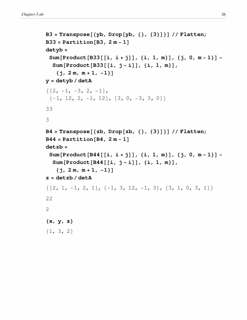
B3 = Transpose@8yb, Drop@yb, 8<, 83<D<D êê Flatten;


detyb =



8j, 2 m, m + 1, −1<D

y = detybêdetA

882, −1, −3, 2, −1<,

8−1, 12, 2, −1, 12<, 83, 0, −3, 3, 0<<

33

3

B4 = Transpose@8zb, Drop@zb, 8<, 83<D<D êê Flatten;


detzb =



8j, 2 m, m + 1, −1<D

z = detzbêdetA

882, 1, −1, 2, 1<, 8−1, 3, 12, −1, 3<, 83, 1, 0, 3, 1<<

22

2

8x, y, z<

81, 3, 2<

Chapter-5.nb 26

5.7 Solving Linear Equations using Iteration Method

Iterative methods are used when the number of equations is large and most of the coeffi-

cients are zero (i.e., a sparse matrix). Iterative methods generally diverge unless the

system of equations is diagonally dominant.

Consider the following linear equations:

a11 x1 + a12 x2 + a13 x3 + ... .. + a1 m xm = a1,m+1

a21 x1 + a22 x2 + a23 x3 + ... .. + a2 m xm = a2,m+1

a31 x1 + a32 x2 + a33 x3 + ... .. + a3 m xm = a3,m+1

.......

am-1,1 x1 + am-1,2 x2 + am-1,3 x3 + ... .. + am-1,m xm = am-1,m+1

am,1 x1 + am,2 x2 + am,3 x3 + ... .. + am,m xm = am,m+1

First, set an initial value for all xi = 0, and solving the first equation for x1, the second

equation for x2, .......up to xm , we get the following set of equations :

x1 = Ha1,m+1 - a12 x20 - a13 x3

0 - ... .. - a1 m xm0 L êa11

x2 = Ha2,m+1 - a21 x1 - a23 x30 - ... .. - a2 m xm

0 L êa22

x3 = Ha3,m+1 - a31 x1 - a32 x2 - a34 x40 - ....-a3 m xm

0 L êa33

................

xi = Hai,m+1 - ai,1 x1 - ai,2 x2 - ... - ai,i-1 xi-1 - ... - ai,i+1 xi+10 - ... -

ai,m-1 xm-10 - ai,m xm

0 L êai,i

................

xm-1 =

Ham-1,m+1 - am-1,1 x1 - am-1,2 x2 - am-1,3 x3 - ... ... - am-1,m-2 xm-2 - am-2,m xm0 L ê

am-1,m-1

xm = H am,m+1 - am,1 x1 - am,2 x2 - am,3 x3 - ... .. - am,m-1 xm-1L êam,m

In general, the set of equations can be written as :

xi = Hai,m+1 -⁄ j=1i-1 ai, j x j -⁄ j=i+1

m ai, j x j0 L êai,i

where x j0 is the assigned old values, and x j are the most newley calculated values.

Chapter-5.nb 27

Example 8

Consider the following system of equations to be solved for x1, x2, ... ... .. x9 using

the Iteration method. Given the equations as:

eq1 : 4 x1 - x2 - x4 = 25 ;

eq2 : - x1 + 4 x2 - x3 - x5 = 5 0 ;

eq3 : -x2 + 4 x3 - x6 = 150 ;

eq4 : -x1 + 4 x4 - x5 - x7 = 0 ;

eq5 : -x2 - x4 + 4 x5 - x6 - x8 = 0 ;

eq6 : -x3 - x5 + 4 x6 - x9 = 50 ;

eq7 : -x4 + 4 x7 - x8 = 0 ;

eq8 : -x5 - x7 + 4 x8 - x9 = 0 ;

eq9 : -x6 - x8 + 4 x9 = 25 ;

Chapter-5.nb 28

Clear@"Global`∗"D

A = 884, −1, 0, −1, 0, 0, 0, 0, 0, 25<,

8−1, 4, −1, 0, −1, 0, 0, 0, 0, 50<,

80, −1, 4, 0, 0, −1, 0, 0, 0, 150<,

8−1, 0, 0, 4, −1, 0, −1, 0, 0, 0<,

80, −1, 0, −1, 4, −1, 0, −1, 0, 0<,

80, 0, −1, 0, −1, 4, 0, 0, −1, 50<,

80, 0, 0, −1, 0, 0, 4, −1, 0, 0<,

80, 0, 0, 0, −1, 0, −1, 4, −1, 0<,

80, 0, 0, 0, 0, −1, 0, −1, 4, 25<<;

m = Length@A D; B = A; n = 50;

eq@i_D := Sum@A@@i, jDD x@jD, 8j, 1, m<D � A@@i, 10DD


Table@x0@iD = 0, 8i, 1, m<D;

x@i_D :=

HB@@i, m + 1DD − Sum@B@@i, jDD x@jD, 8j, 1, i − 1<D −

Sum@A@@i, jDD x0@jD, 8j, i + 1, m<DL êB@@i, iDD

For@k = 1, k ≤ n, k++, 8For@i = 1, i ≤ m, i++, x@iDD,

Table@x0@iD = x@iD, 8i, 1, m<D<D


Chapter-5.nb 29

4 x@1D − x@2D − x@4D � 25

−x@1D + 4 x@2D − x@3D − x@5D � 50

−x@2D + 4 x@3D − x@6D � 150

−x@1D + 4 x@4D − x@5D − x@7D � 0

−x@2D − x@4D + 4 x@5D − x@6D − x@8D � 0

−x@3D − x@5D + 4 x@6D − x@9D � 50

−x@4D + 4 x@7D − x@8D � 0

−x@5D − x@7D + 4 x@8D − x@9D � 0

−x@6D − x@8D + 4 x@9D � 25

818.75, 37.5, 56.25, 12.5, 25., 37.5, 6.25, 12.5, 18.75<

Compare with the Guassian elemination method

Chapter-5.nb 30

Mathematica Solution 2

Clear@"Global`∗"D

A = 884, −1, 0, −1, 0, 0, 0, 0, 0, 25<,

8−1, 4, −1, 0, −1, 0, 0, 0, 0, 50<,

80, −1, 4, 0, 0, −1, 0, 0, 0, 150<,

8−1, 0, 0, 4, −1, 0, −1, 0, 0, 0<,

80, −1, 0, −1, 4, −1, 0, −1, 0, 0<,

80, 0, −1, 0, −1, 4, 0, 0, −1, 50<,

80, 0, 0, −1, 0, 0, 4, −1, 0, 0<,

80, 0, 0, 0, −1, 0, −1, 4, −1, 0<,

80, 0, 0, 0, 0, −1, 0, −1, 4, 25<<;

m = Length@A D;



For@j = 1, j ≤ m − 1, j++,

8Which@A@@j, jDD == 0,

88A@@jDD, A@@j + 1DD< = 8A@@j + 1DD, A@@jDD<< D,

For@i = j + 1, i ≤ m, i++, A@@iDD =

A@@iDD − A@@jDD A@@i, jDD ê A@@j, jDD êê ChopD<D



For@i = m − 1, i ≥ 1, i−−, x@iD =


A@@i, iDDD


Chapter-5.nb 31

4 x@1D − x@2D − x@4D � 25

−x@1D + 4 x@2D − x@3D − x@5D � 50

−x@2D + 4 x@3D − x@6D � 150

−x@1D + 4 x@4D − x@5D − x@7D � 0

−x@2D − x@4D + 4 x@5D − x@6D − x@8D � 0

−x@3D − x@5D + 4 x@6D − x@9D � 50

−x@4D + 4 x@7D − x@8D � 0

−x@5D − x@7D + 4 x@8D − x@9D � 0

−x@6D − x@8D + 4 x@9D � 25

4 −1 0 −1 0 0 0

0 15��4

−1 − 1��4

−1 0 0

0 0 56��15

− 1��15

− 4��15

−1 0

0 0 0 209��56

− 15��14

− 1��56

−1

0 0 0 0 712��209

− 225��209

− 60��209

0 0 0 0 0 2415��712

− 17��178

0 0 0 0 0 0 8948��2415

0 0 0 0 0 0 0

0 0 0 0 0 0 0

818.75, 37.5, 56.25, 12.5, 25., 37.5, 6.25, 12.5, 18.75<

5.8 Problems

Problem 1

Solve the following set linear equations the Gaussian elimination and backward substitu-

tion method.

2 x1 - 3 x2 - x3 = -3 ;

-x1 + 2 x2 + x3 = -2 ;

3 x1 - 2 x2 + 3 x3 = 4 ;

Chapter-5.nb 32

Problem 2

Solve the following set linear equations the Gauss Gordon elimenation method.

2 x1 - 3 x2 - x3 = -3 ;

-x1 + 2 x2 + x3 = -2 ;

3 x1 - 2 x2 + 3 x3 = 4 ;

Problem 3

Solve the following linear set of equations by calculating the matrix inversion using

Gauss Jordon elimenation method to evaluate x1, x2, and x3.

2 x1 - 3 x2 - x3 = -3 ;

-x1 + 2 x2 + x3 = -2 ;

3 x1 - 2 x2 + 3 x3 = 4 ;

Problem 4

Solve the following linear set of equations using the determinant method and Cramer's

rule to evaluate x1, x2, and x3. Use numerical algorithm (in chapter 5) to evaluate the

determinants.

2 x1 - 3 x2 - x3 = -3 ;

-x1 + 2 x2 + x3 = -2 ;

3 x1 - 2 x2 + 3 x3 = 4 ;

Problem 5

Solve the following linear set of equations using the eteration method to evaluate

x1, x2, and x3.

2 x1 - 3 x2 - x3 = -3 ;

-x1 + 2 x2 + x3 = -2 ;

3 x1 - 2 x2 + 3 x3 = 4 ;

Chapter-5.nb 33

Computational Physics Chapter 5 Numerical Solution of Linear System of Equations

Documents

Transcript of Computational Physics Chapter 5 Numerical Solution of Linear System of Equations