Differential Equations coursework
45
DIFFERENTIAL EQUATIONS GIANG B KHUONG Contents 1. What is Ordinary Differential Equations (ODE)? 2 2. Basic/Logistic Model and Its Modification 3 3. What is a solution? 5 4. Initial Value Problems (IVP) 8 5. Fundamental Theorem of Ordinary Differential Equations (FTODE) 10 6. Slope Field 11 7. Numerical Method: Euler’s Method 14 8. Linearization of Systems of Differential Equations 16 9. Superposition: Characteristic property of linear equations 19 10. Eigenvalues, eigenvectors, and eigen solutions 22 11. Nullclines 36 12. Oscillations 39 13. Conserved and Monotone Quantities 41 14. Analytic methods 43 1
Transcript of Differential Equations coursework

DIFFERENTIAL EQUATIONS
GIANG B KHUONG
Contents
1. What is Ordinary Differential Equations (ODE)? 2
2. Basic/Logistic Model and Its Modification 3
3. What is a solution? 5
4. Initial Value Problems (IVP) 8
5. Fundamental Theorem of Ordinary Differential Equations (FTODE) 10
6. Slope Field 11
7. Numerical Method: Euler’s Method 14
8. Linearization of Systems of Differential Equations 16
9. Superposition: Characteristic property of linear equations 19
10. Eigenvalues, eigenvectors, and eigen solutions 22
11. Nullclines 36
12. Oscillations 39
13. Conserved and Monotone Quantities 41
14. Analytic methods 43
1

2 GIANG B KHUONG
1. What is Ordinary Differential Equations (ODE)?
Ordinary Differential Equations (or ODEs) are equations with derivatives in them, and
where unknowns are functions.
Example:
Q = population of orchids in garden, in thousands
t = time, in weeks
dQ
dt= 0.8Q(1− Q
12)− 0.12Q
To build differential equations:
• make assumptions on which the model will be based
• describe variables and parameters to be used
• translate into math symbols
Example:
The rate of change of the orchid population is precisely 1500/week
P = orchid population, in thousands
t = time, in weeks
dP
dt= 7
The unknown is the function P (t).

DIFFERENTIAL EQUATIONS 3
2. Basic/Logistic Model and Its Modification
(1) Basic Models
Basic models of population growth are based on the assumptions that the rate
of growth of the population is proportional to the size of the population.
dP
dt= rP
where r is the constant rate of growth, and P is the population.
Example:
The rate of change of fish in river A annually is exactly 15%.
F = fish population in river A, in thousands
t = time, in years
dF
dt= 0.15F
(2) Logistic Models
Logistic models are based on the assumptions that the rate of growth of the
population is proportional to the size of the population but that increase may be
limited, e.g. growth rate of fish depends on the availability of volume of water.
dP
dt= rP (1− P
K)
where r is the constant rate of growth, and K is the availability of habitat.
Example:
The growth rate of aphids in kale patch is 7% per week. The kale patch can
sustain a maximum of 1.5 million aphids.
A = aphid population, in thousands
4 GIANG B KHUONG
t = time, in weeks
dA
dt= 0.07A(1− A
1500)
(3) Modifications of Logistic Models
(a) Harvesting: −f(P )
Example:
The growth rate of aphids in kale patch is 7% per week. The kale patch
can sustain a maximum of 1.5 million aphids.
Also, the aphids are harvested at a constant rate of 10% per week.
A = aphid population, in thousands
t = time, in weeks
dA
dt= 0.07A(1− A
1500)− 0.1A
(b) Hatchery: +f(P )
Example:
The growth rate of fish in river A monthly is 2%. The river can sustain
up to 15,000 fish.
Environmentalists are trying to replenish the fish stock in that river by
releasing 5,000 fish in the river every month.
F = fish population in river A, in thousands
t = time, in years
dF
dt= 0.2F (1− F
15) + 5

DIFFERENTIAL EQUATIONS 5
3. What is a solution?
As mentioned before, solutions to ODEs are functions, instead of numbers like in alge-
braic equations.
A function is a solution to an ODE if the equation is true when we plug it in.
Example:
Proof that y(t) = 42e0.5t is a solution to
ODE1 =dy
dt= 0.5y
Proof:
LHS =d
dt[y(t)] =
d
dt(42e0.5t) = 42(0.5)e0.5t = 21e0.5t
RHS = 0.5y = (0.5)(42e0.5t) = 21e0.5t
LHS = RHS
Hence, y(t) = 42e0.5t is a solution to ODE1.
General Solutions
Example:
There is a collection of functions in the form y(t) = Ce0.5t to ODE1, where C is a
constant.
Proof:
LHS =d
dt[y(t)] =
d
dt(Ce0.5t) = (0.5)(Ce0.5t)

6 GIANG B KHUONG
RHS = 0.5y = (0.5)(Ce0.5t)
LHS = RHS
Hence, y(t) = Ce0.5t is a solution to ODE1, where C is any constant.
Graph:
Figure 1. C = −2,−1, 0, 1, 2
Observation:
Any point on the plane lies one exactly one solution curve.
General features of general solutions:
• lots of solutions
• the solutions fill the plane

DIFFERENTIAL EQUATIONS 7
.
Equilibrium Solutions
Equilibrium solutions are constant functions. The interpretation of such functions is
steady-state, i.e. no dynamics.
(1) Equilibrium solutions of Basic models
Example:
Consider the following basic growth model
dP
dt= 0.7P
For equilibrium solutions, P (t) = constant, hence dPdt = 0
0 = 0.7P
P (t) = 0
P (t) = 0 is the equilibrium solution for this basic growth model.
(2) Equilibrium solutions of Logistic models
Example:
Consider this logistic growth model
dP
dt= 0.7P (1− P
9)
For equilibrium solutions, P (t) = constant, hence dPdt = 0
0 = 0.7P (1− P
9)

8 GIANG B KHUONG
either P = 0 or 1− P9 = 0
P (t) = 0 andP (t) = 9 are the equilibrium solutions for this logistic model.
(3) Equilibrium solutions of Logistic models with modifications
Example:
Consider this modified logistic growth model
dP
dt= 0.7P (1− P
9) + 2
For equilibrium solutions, P (t) = constant, hence dPdt = 0
0 = 0.7P (1− P
9) + 2
0 = 0.7P − 0.07
9P 2 + 2
0 = P 2 − 15P − (15
0.07)2
either P = −15 or P = 30
P (t) = −15 andP (t) = 30 are the equilibrium solutions for this modified logistic
model.
4. Initial Value Problems (IVP)
For equations of the formdy
dt= f(t, y)
it seems like there are many solutions; in fact, the solutions fill the plane, i.e. each point
(tA, yA) lies on a solution.
So, given an equation, does there exist a solution? If so, is this solution unique?

DIFFERENTIAL EQUATIONS 9
An Initial Value Problem (IVP) put additional requirement so that to satisfy an IVP,
the solution graph has to pass through a point on the plane. This makes IVP have one
unique solution.
Example:
Find y(t) such that
dydt = f(t, y)
y(to) = yo
y(t) will not only be solution to the ODE, but it will also satisfy the additional requirement
to pass through (to, yo). Note: that to can be any arbitrary starting point t.
Example:
Consider the following IVP:
dydt = cos (t)
y(0) = 7
Solve:
First look at ODE dydt = cos (t)
y(t) = sin (t) + C
is a solution for any C.
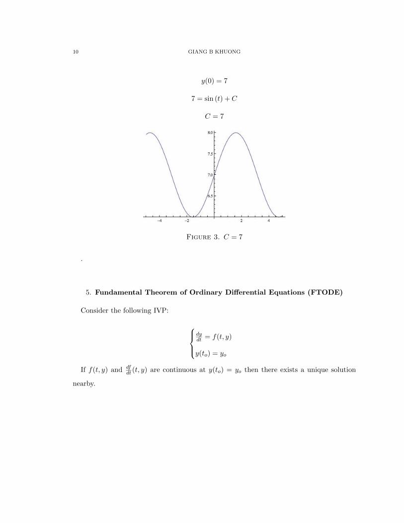
Figure 2. C = −5, 0, 7
10 GIANG B KHUONG
y(0) = 7
7 = sin (t) + C
C = 7
Figure 3. C = 7
.
5. Fundamental Theorem of Ordinary Differential Equations (FTODE)
Consider the following IVP:
dydt = f(t, y)
y(to) = yo
If f(t, y) and dfdt (t, y) are continuous at y(to) = yo then there exists a unique solution
nearby.

DIFFERENTIAL EQUATIONS 11
Example:
dydt = t3 cos (y)
y(1) = π
Here f(t, y) = t3 cos (y)
• is this continuous near (t, y) = (1, π)?
• look at dfdt (t, y) = t3(− sin (y))
is this continuous near (1, π)?
Both questions have answers ”Yes”, which means that there exists a function y(t) such
that:
• y(t) = π
• y is defined for t nearby t = 1
• dydt = t3 cos (y)
• there is only one such function
Important consequences:
We cannot have two solutions meet.
6. Slope Field
The ODE tells us the slope of the function. This gives us a sense of what the growth
looks like.
We can use that information to plot a slope field.
Example:
(1) Basic Growth Model
dP
dt= rP

12 GIANG B KHUONG
(a) r > 0
Figure 4. r > 0
P = 0, slope = 0
P = 1, slope = r
P = 2, slope = 2r
These slopes are independent of t. At each point on the t-p plane, we have a
slope.
The slope arrows are tangent to any solution curve, i.e. solutions follow the
slope values.
Thus slope field tells us what graphs of solutions look like.

DIFFERENTIAL EQUATIONS 13
(b) r < 0
Figure 5. r < 0
Initial conditions nearby to P = 0 have solutions which approach P = 0
Terminology:
• If nearby solutions approach an equilibrium, we say that the equilibrium is stable.
• If nearby solutions diverge from an equilibrium, we say that the equilibrium is unstable.

14 GIANG B KHUONG
(2) Logistic Model
dP
dt= rP (1− P
K)
r > 0,K > 0
Figure 6. Equilibrium at P = 0 and P = K
P = 0, slope = 0
P = K, slope = 0
P = 2K, slope = r(2K)(1− 2KK ) = −2Kr
P (t) = 0 is an unstable equilibrium because nearby solutions diverge from P = 0.
P (t) = K is an stable equilibrium because nearby solutions converge towards
P = K.
.
7. Numerical Method: Euler’s Method
Euler’s Method approximate numerically the change of y as t changes a ∆t, as oppose
to the slope field, which offers a graphical approximation.
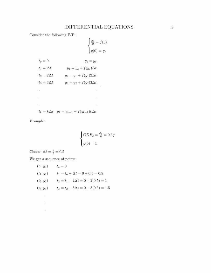
DIFFERENTIAL EQUATIONS 15
Consider the following IVP: dydt = f(y)
y(0) = yo
to = 0 yo = yo
t1 = ∆t y1 = yo + f(yo)∆t
t2 = 2∆t y2 = y1 + f(y1)2∆t
t3 = 3∆t y3 = y2 + f(y2)3∆t
. .
. .
. .
tk = k∆t yk = yk−1 + f(yk−1)k∆t
.
Example:
ODE2 = dy
dt = 0.3y
y(0) = 1
Choose ∆t = 12 = 0.5
We get a sequence of points:
(to, yo) to = 0
(t1, y1) t1 = to + ∆t = 0 + 0.5 = 0.5
(t2, y2) t2 = t1 + 2∆t = 0 + 2(0.5) = 1
(t3, y3) t3 = t2 + 3∆t = 0 + 3(0.5) = 1.5
.
.
.

16 GIANG B KHUONG
8. Linearization of Systems of Differential Equations
(1) Why should we linearize a system of ODEs?
Linear equations are continuous, hence it is easy to solve IVPs to these equations.
Example:
ODE = dy
dt = 3y
y(0) = A
General solution: y(t) = Ce3t
y(0) = Ce3(0) = C
Hence, C = A
The solution to this IVP is y(t) = Ae3t
Linearization is trying to approximate non-linear equations at a certain point.
Usually we choose the equilibrium point to get an approximated linear equation for
a new variable which represents the deviation from the equilibrium.
(2) How to linearize systems of ODEs?
If we have a non-linear function f(yk), it can be locally approximated by a
straight line.

DIFFERENTIAL EQUATIONS 17
g(y) = f(yk) + f ′(yk)(y − yk)
We say that g(y) approximates f(y) near yk
f(y) = f(yk) + f ′(yk)(y − yk) + ...
We usually call this the Taylor series.
The linearization of f at yk is linear part of the Taylor series f(y) ≈ f(yk) +
f ′(yk)(y − yk)
By Linearization of Systems of ODEs, we can learn ’essentially everything’ we
want to know near any equilibrium yk by looking at the linearization.
dxdt = f(x, y)
dydt = g(x, y)
To approximate f(x, y) near some point (xA, yA):
f(x, y) ≈ f(xA, yA) +df
dx(xA, yA)(x− xA) +
df
dy(xA, yA)(y − yA)
Example:
Linearize the following system at (2, 6)
dxdt = 0.08x(1− x
8 )− 0.01xy
dydt = 0.04y − 0.02xy
• f(2, 6) = 0.16(34)− 0.12
dfdx = 0.08(1− x
8 )+0.08x(18)−0.01y → dfdx(2, 6) = 0.06−0.02−0.06 = 0.02
dfdy = −0.01x → df
dy (2, 6) = −0.02
f(x, y) ≈ 0 + (−0.02)(x− 2) + (−0.02)(y − 6)
• g(2, 6) = 0.04(6)− 0.02(2)(6)
dgdx = −0.02y → dg
dx(2, 6) = −0.12

18 GIANG B KHUONG
dgdy = 0.04− 0.02x → dg
dy (2, 6) = 0.04− 0.02(2) = 0
g(x, y) ≈ 0 + (−0.12)(x− 2) + 0(y − 6)
∴
dxdt ≈ −0.02(x− 2)− 0.02(y − 6)
dydt ≈ 0.12(x− 2)
(3) How to analyze properties of systems of ODEs via linearization?
The system of ODEs
dxdt = ax+ by
dydt = cx+ dy
can be written in matrix form as follow:
d
dt
xy
=
ax+ by
cx+ dy
=
ax+ by
cx+ dy
=
a b
c d
xy
Let
xy
= ~y we have:
d
dt~y =
a b
c d
~yTo check whether a function is a solution to a linearized system of ODEs or not,
just plug it in.
Example:
d
dt~y =
2 3
7 6
~yShow that ~y1(t) = e−t
−1
1
and ~y1(t) = e9t
3
7
are solutions.

DIFFERENTIAL EQUATIONS 19
(a) Examine ~y1(t) = e−t
−1
1
LHS = d
dt [~y1(t)] = −e−t−1
1
= e−t
1
−1
RHS =
2 3
7 6
e−t−1
1
= e−t
1
−1
LHS = RHS
∴ ~y1(t) = e−t
−1
1
is a solution.
(b) Examine ~y1(t) = e9t
3
7
LHS = d
dt [~y2(t)] = 9e9t
3
7
= e9t
27
63
RHS =
2 3
7 6
e9t3
7
= e9t
27
63
LHS = RHS
∴ ~y2(t) = e9t
3
7
is a solution.
9. Superposition: Characteristic property of linear equations
(1) Superposition Theorem:
If y1 and y2 are solutions to a linear equation, then αy1 + βy2 is also a solution
to the linear equation for all number α, β.
The quantity αy1 + βy2 is called a linear combination (of y1 and y2)

20 GIANG B KHUONG
Example:
Assume that w1 and w2 solve:
dw
dt= rw
Examine αw1 + βw2
d
dt[αw1 + βw2] = α
dw1
dt+ β
dw2
dt= α(rw1) + β(rw2) = r(αw1 + βw2)
This works because multiplication and derivation share some properties.
(2) Application of the Superposition theorem:
We can use the Superposition theorem to generate a general solution form from
a few solutions.
Example 1:
We know from example in Section 8, number (3) that ~y1(t) = e−t
−1
1
and
~y1(t) = e9t
3
7
are solutions for the system:
d
dt~y =
2 3
7 6
~yBy the Superposition theorem,
Y (t) = α~y1(t) + β ~y2(t)
i.e. Y (t) = αe−t
−1
1
+ βe9t
3
7

DIFFERENTIAL EQUATIONS 21
Example 2:
Solve the following IVP:
ddt~y =
2 3
7 6
~yy(0) =
1
9
We know that
Y (t) = αe−t
−1
1
+ βe9t
3
7
is a solution for all α, β.
→ Find α, β to match initial condition.
We want1
9
= αe−(0)
−1
1
+ βe9(0)
3
7
1
9
= α
−1
1
+ β
3
7
1
9
=
−α+ 3β
α+ 7β
We then need to solve:
1 = −α+ 3β
9 = α+ 7β
Adding the two equations give: 10 = 10β
β = 1
1 = −α+ 3(1)

22 GIANG B KHUONG
−2 = −α
α = 2
∴ Y (t) = 2e−t
−1
1
+ e9t
3
7
solves the IVP.
10. Eigenvalues, eigenvectors, and eigen solutions
(1) Transforming the linearized problems into eigenvalue problems
From last chapter, we had a linearized, first order ODE:
d
dt~y =
a b
c d
~yWe look for solutions of the form:
~y(t) = eλt
xy
where λ, x, y are real numbers.
Assuming that ~y(t) solves the ODE, we have:
λeλt
xy
=
a b
c d
eλtxy
Since eλt 6= 0, we can divide by eλt. We then want λ
xy
such that:
a b
c d
xy
= λ
xy
We now have an eigenvalue problem. Find constant λ and vector ~V such that:
a b
c d
~V = λ~V

DIFFERENTIAL EQUATIONS 23
λ is called the eigenvalue.
~V is called the eigenvector.
Given the matrix, we can find the eigenvalue λ and the associated eigenvector
~V . Then we can can form the solution eλt~V .
(2) How to solve eigenvalue problem
Take the example from the previous section:
a b
c d
xy
= λ
xy
a b
c d
xy
− λxy
=
0
0
Observe that the matrix
λ 0
0 λ
has the same effect as the scalar quantity λ.
∴
a b
c d
xy
−λ 0
0 λ
xy
=
0
0
a b
c d
−λ 0
0 λ
xy
=
0
0
In general, we have:
a− λ b
c d− λ
xy
=
0
0
We do not want x = y = 0, hence we are looking for non-trivial solutions for
this system. For non-trivial solutions to exist, the determinant
∣∣∣∣∣∣a− λ b
c d− λ
∣∣∣∣∣∣ has
to be equal to zero.

24 GIANG B KHUONG
i.e.
(a− λ)(d− λ)− bc = 0
We solve the quadratic equation for λ1 and λ2. To find the associated eigenvector,
plug the found λ back into the eigenvalue problem.
a b
c d
xy
= λ1
xy
ax+ by = λ1x
cx+ dy = λ1y
Then choose a pair of x, y that satisfies the pair of equations. That is the
associated eigenvector ~V1 for λ1. Do the same for λ2
We, then, have two ”eigen” solutions eλ1t ~V1 and eλ2t ~V2.
By the principle of superposition, we have the general solution:
~Y (t) = αeλ1t ~V1 = βeλ2t ~V2
Example: Find the general solution for the following ODE.
d
dt~y =
2 1
1 2
~y1. Find eigenvalues λ1, λ22 1
1 2
xy
= λ
xy
2 1
1 2
xy
−λ 0
0 λ
xy
=
0
0
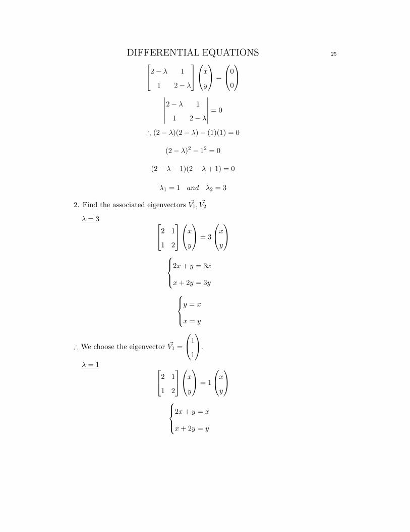
DIFFERENTIAL EQUATIONS 252− λ 1
1 2− λ
xy
=
0
0
∣∣∣∣∣∣2− λ 1
1 2− λ
∣∣∣∣∣∣ = 0
∴ (2− λ)(2− λ)− (1)(1) = 0
(2− λ)2 − 12 = 0
(2− λ− 1)(2− λ+ 1) = 0
λ1 = 1 and λ2 = 3
2. Find the associated eigenvectors ~V1, ~V2
λ = 3 2 1
1 2
xy
= 3
xy
2x+ y = 3x
x+ 2y = 3yy = x
x = y
∴ We choose the eigenvector ~V1 =
1
1
.
λ = 1 2 1
1 2
xy
= 1
xy
2x+ y = x
x+ 2y = y

26 GIANG B KHUONGy = −x
x = −y
∴ We choose the eigenvector ~V1 =
1
−1
.
We, then, have two ”eigen” solutions e3t
1
1
and et
1
−1
.
By the principle of superposition, we have the general solution:
~Y (t) = αe3t
1
1
+ βet
1
−1
Figure 7. Phase Plane Plot
For IVPs, solve for specific α, β.

DIFFERENTIAL EQUATIONS 27
(3) Real eigenvalues
There are three cases for real eigenvalues λ:
• λ1 is positive and λ2 is negative
• both λ1 and λ2 are positive
• both λ1 and λ2 are negative
Case 1: One λ is positive and one λ is negative
d
dt~y =
3 8
3 5
~yλ1 = 9 and λ2 = −1
Associated eigenvectors are ~V1 =
4
3
and ~V2 =
−2
1
The general solution is ~Y (t) = αe9t
4
3
+ βe−t
−2
1
Figure 8. λ1 > 0, λ2 < 0

28 GIANG B KHUONG
The two straight lines are the eigenvectors. In this case, we have one going in
(towards (0, 0)), corresponding to λ < 0 and one going out (away from (0, 0)),
corresponding to λ > 0.
This configuration is called a saddle.
Case 2: Both λ1 and λ2 are positive
d
dt~y =
5 0
17 3
~yλ1 = 5 and λ2 = 3
Associated eigenvectors are ~V1 =
2
17
and ~V2 =
0
1
The general solution is ~Y (t) = αe5t
2
17
+ βe3t
0
1
Figure 9. λ1 > 0, λ2 > 0
DIFFERENTIAL EQUATIONS 29
Here, we have both eigenvector going out (away from (0, 0)), corresponding to
both λ > 0.
This configuration is called a source.
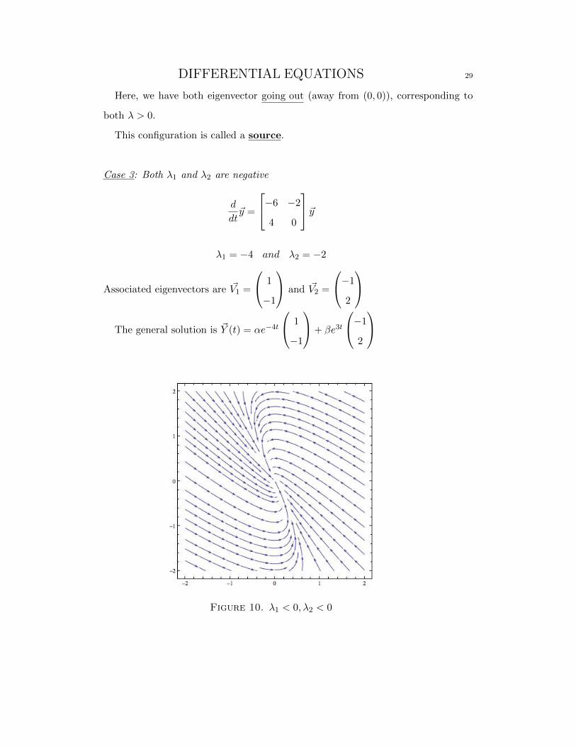
Case 3: Both λ1 and λ2 are negative
d
dt~y =
−6 −2
4 0
~yλ1 = −4 and λ2 = −2
Associated eigenvectors are ~V1 =
1
−1
and ~V2 =
−1
2
The general solution is ~Y (t) = αe−4t
1
−1
+ βe3t
−1
2
Figure 10. λ1 < 0, λ2 < 0

30 GIANG B KHUONG
In this case, we have both eigenvector going in (towards (0, 0)), corresponding
to both λ < 0.
This configuration is called a sink.
(4) Complex/unreal eigenvalues
(a) Tools to understand complex solutions
(i) What is a complex number?
A complex number is a number that can be put in the form a + bi,
where a and b are real numbers and i is called the imaginary unit, where
i2 = −1.
Example:
λ2 + 4 = 0
λ2 = −4
λ = ±2i
If we include i in our world, all quadratic can be solved:
aλ2 + bλ+ c = 0
λ =−b±√b2 − 4ac
2a
If b2 − 4ac ≥ 0, then we have our usual real solutions.
If b2 − 4ac ≤ 0, then we have complex solutions.
All usual algebra works for complex numbers.

DIFFERENTIAL EQUATIONS 31
(ii) Euler’s Formula
We can express eit as:
eit = cos(t) + i sin(t)
This is from Taylor’s series expansion.
eit = 1 +it
1!+it2
2!+it3
3!+it4
4!...
= 1 + it− t2
2!+it3
3!+t4
4!+it5
5!...
= (1− t2
2!+t4
4!− ...) + i(t+
t3
3!+t5
5!...)
= cos t+ i sin t
(b) Solve for complex eigenvalues
d
dt~y =
1 1
−5 3
~y(1− λ)(3− λ) + 5 = 0
λ1 = 2 + 2i and λ2 = 2− 2i
λ1 = 2 + 2i 1 1
−5 3
xy
= (2 + 2i)
xy
x+ y = (2 + 2i)x
−5x+ 3y = (2 + 2i)y
y = (1 + 2i)x
∴ ~V1 =
1
1 + 2i

32 GIANG B KHUONG
The first eigen solution is:
~Y1(t) = e(2+2i)t
1
1 + 2i
= e2te2it
1
1 + 2i
= e2t(cos(2t) + i sin(2t))
1
1
+ i
0
2
=
e2t cos(2t)
1
1
− e2t sin(2t)
0
2
+ i
e2t cos(2t)
0
2
+ e2t sin(2t)
1
1
λ1 = 2− 2i 1 1
−5 3
xy
= (2− 2i)
xy
x+ y = (2− 2i)x
−5x+ 3y = (2− 2i)y
y = (1− 2i)x
∴ ~V2 =
1
1− 2i

DIFFERENTIAL EQUATIONS 33
The second eigen solution is:
~Y2(t) = e(2−2i)t
1
1− 2i
= e2te−2it
1
1− 2i
= e2t(cos(−2t) + i sin(−2t))
1
1
− i0
2
=
e2t cos(2t)
1
1
− e2t sin(2t)
0
2
− ie2t cos(2t)
0
2
+ e2t sin(2t)
1
1
Observation:
• eigenvalues come in pairs λ = a± bi
• eigenvectors come in pairs ~V = ~Vreal + ~Vimaginary
• eigen solutions come in pairs
General solution:
~Y (t) = α ~Y1(t) + β ~Y2(t)
= (α+ β)
e2t cos(2t)
1
1
− e2t sin(2t)
0
2
+ i(α− β)
e2t cos(2t)
0
2
+ e2t sin(2t)
1
1
Set α = β = 12 , we have REAL ~Y (t) =
e2t cos(2t)
1
1
− e2t sin(2t)
0
2
Set α = 1
2i , β = −12i , we have REAL ~Y (t) =
e2t cos(2t)
0
2
+ e2t sin(2t)
1
1
34 GIANG B KHUONG
We can then generate another general solution:
~Y (t) = A
e2t cos(2t)
1
1
− e2t sin(2t)
0
2
+B
e2t cos(2t)
0
2
+ e2t sin(2t)
1
1
⇒ If eigenvalues λ are complex, then both the real and imaginary part of ~Y1(t)
or ~Y2(t) are REAL solutions which can be used to form REAL general solution.
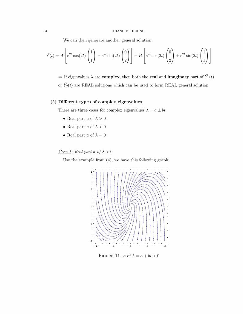
(5) Different types of complex eigenvalues
There are three cases for complex eigenvalues λ = a± bi:
• Real part a of λ > 0
• Real part a of λ < 0
• Real part a of λ = 0
Case 1: Real part a of λ > 0
Use the example from (4), we have this following graph:
Figure 11. a of λ = a+ bi > 0

DIFFERENTIAL EQUATIONS 35
This configuration is called spiral source since all solutions are moving away
from the center (0, 0).
Case 2: Real part a of λ < 0
d
dt~y =
−1 −1
−1 0
~yλ = −1
2± i√
3
2
Figure 12. a of λ = a+ bi > 0
This configuration is called spiral sink since all solutions are moving towards
the center (0, 0).

36 GIANG B KHUONG
Case 3: Real part a of λ = 0
d
dt~y =
1 2
−5 −1
~yλ = ±3i
Figure 13. a of λ = a+ bi > 0
11. Nullclines
Definition:
Nullclines offer a way to analyze ODEs behavior in between equilibrium points. This
gives a more general behavior of the ODEs than qualitative analysis like linearization and
eigenstuffs analysis.
For any system dxdt = f(x, y)
dydt = g(x, y)

DIFFERENTIAL EQUATIONS 37
the x-nullcline is the set of points (x, y) where f(x, y) is zero, i.e. the level curve where
f(x, y) is zero. Similarly, the y-nullcline is the set of points where g(x, y) is zero.
Along the x-nullcline,the x-component of the vector field is zero, hence, the vector field
is vertical, i.e. either pointing straight up or straight down. Similarly, the vector field along
the y-nulcline will be pointing either right or left, since its y-component is zero.
The intersections of these nullclines are the equilibria. because both f(x, y) and g(x, y)
are zero at equilibria.
Example:
Consider the following system:
dxdt = 2x(1− x
2 )− xy)
dydt = −y + xy
Using the normal linearization and eigenstuffs analysis yield the following phase plane:
Figure 14. Assemble phase plane around equilibria

38 GIANG B KHUONG
The nullclines phase plane of this system of ODEs is the skeleton of the behavior, as
shown below:
Figure 15. Nullclines phase plane
Assemble both phase plane results in the following picture:
Figure 16. Final phase plane

DIFFERENTIAL EQUATIONS 39
12. Oscillations
According to Newton’s second law of motion, we have the equation:
F = ma = md2y
dt2
where m =mass (constant) and y = position as a function of time.
Hooke’s law also offered another force model for describe mass on springs, where:
Together, we have:
F = md2y
dt2= −ky
Rearranging the equation, we have:
d2y
dt2+k
my = 0
This is called the Simple Harmonic Oscillator (SHO).
The general form of SHO is the second order linear ODE:
md2y
dt2+ b
dy
dt+ ky = f(t)
where md2ydt2
is the factor from Newton’s law, bdydt is the damping factor, ky is the oscillating
factor, and f(t) is the external force factor; or the forcing/driving factor.
When f(t) = 0, the system is called homogeneous; otherwise, it is called inhomoge-
neous.
To analyze the second order SHO, we need to convert the second order equation to
a system of first order ODEs. Then, we can use our normal qualitative methods like
linearization and eigenstuffs analysis.
To convert this second order SHO to a first order system of ODEs, we need to introduce
a new variable v = dydt . This make d2y
dt2= dv
dt .

40 GIANG B KHUONG
We obtain the system:
dydt = v
mdvdt + bv + ky = f(t)
For homogeneous system, we guess the solution to be in the form of yh(t) = eλt. We,
then pluck this guess into the equations to check and figure out λ. We work out the general
homogeneous solution using normal method of eigenvalues λ and eigenvectors.
For inhomogeneous system, the solution is made up of 2 parts: the homogeneous and
the particular solution, i.e. y(t) = yh(t) + yp(t). This works because of the Superposition
theorem discussed in chapter 9.
We find the homogeneous solution by setting the equation equals to zero, and use the
same method as solving homogeneous equation. For example, we have inhomogeneous
equation:
md2y
dt2+ b
dy
dt+ ky = f(t)
We find the homogeneous part of the solution by setting
md2y
dt2+ b
dy
dt+ ky = 0
and using the guessing method as discussed above.
For the particular part of the solution, we guess the solution to be in the form of the
forcing factor, i.e. in the form of whatever f(t) is.
For example, if f(t) = 7t, then the particular solution is in the form yp(t) = A+ Bt; if
f(t) = e−10t, then yp(t) = Aert; if f(t) = cos 3t, then yp(t) = A cos 3t+B sin 3t, etc.

DIFFERENTIAL EQUATIONS 41
13. Conserved and Monotone Quantities
Conserved Quantities
A quantity is conserved along a solution curve in the phase plane if ddt(quantity) = 0
An example of conserved quantity is is energy, as studied in Physics, which consists of
kinetic energy, which measures how large velocity is, and potentl energy, which measures
the energy inherent in the position of the system.
E =1
2mv2 + V (y)
where 12mv
2 is kinetic energy and V (y) is potential energy.
d
dt[E] =
d
dt
(1
2mv2 + V (y)
)= mv
dv
dt+ V ′(y)
dy
dt(dy
dt= v and
dy
dt= − k
my)
= v
(m−kmy + V ′(y)
)= v
(−ky + V ′(y)
)The quantity E is conserved if d
dt [E] = 0, which happens when V (y) = ky. We then
choose V (y) = 12ky
2 so that E is conserved.
Thus, we have the conserved quantity
E =1
2mv2 +
1
2ky2
However, there are many different conserved quantity, depends on the system of SHO.
We can draw the energy plane and phase plane of the SHO with conserved quantity as
following:

42 GIANG B KHUONG
Figure 17. Energy plane: V (y)
Figure 18. Phase plane y − v
The energy and phase plane above can be describing a mass attached to a spring, sliding
on ice, i.e. no friction/damping: At whatever initial displacement y0 from equilibrium the
mass was set, it will oscillate between y0 and −y0 forever, because there is no damping and
no forcing acting on the system (the reason why the phase plane is a circle.)
Analyzing the energy diagram’s behavior:
We have the initial condition: at t = 0, (y0, v0)
E0 =1
2y0
+ 1
2v0
2

DIFFERENTIAL EQUATIONS 43
E is conserved, hence the solutions stay on whatever initial E = E0.
If V0 is greater than 0, then initially y increases until solution runs into the curve given
by V (y). If the system stop at this point then that point is an equilibrium.
If this point is not an equilibrium then dydt is negative, and y begins to decreases until it
hits the other side of the solution.
Look at Figure 17. Our solutions oscillates at height E0 between potential walls. If t0
was large then it will oscillate at a higher altitude decreases.
If the solution/quantity oscillates but either decreases or increases, then it is called a
monotone quantity.
14. Analytic methods
Separation of variables:
We may work out the general solution by re-arranging equation to separate the variables,
and integrate both sides.
Example:
dy
dt= et cos (y)
1
eydy
dt= cos (y)
e−ydy
dt= cos (y)∫ T
te−y
dy
dtdt =
∫ T
tcos (y)dx (y0 = y(t0))
−e−t∣∣∣y(T )y(t0)
= sin (t)∣∣∣Tt0
e−y(T ) = − sin (T ) + sin (t0) + e−y0
y(T ) = − ln(− sin (T ) + sin (t0) + e−y0
)

44 GIANG B KHUONG
We can set sin (t0) + e−y0 = C, since this is just some constant that are determined by
initial condition (t0, y0).
Our final solution is
y(t) = − ln [C − sin (t)]
Usage on Logistic Model:
dPdt = rP
(1− P
K
)P (0) = P0
We now see that dPdt = rP
(1− P
K
)is separable.
dP
dt= rP
(1− P
K
)1
P(1− P
K
) dPdt
= r
∫ T
0
1
P(1− P
K
) dPdtdt =
∫ T
0rdt
∫ PT
P0
1
P(1− P
K
) dPdt
= rT
We now need to find an anti-derivative for 1P(1− P
K )by partial fractions, as we have known
from Calc II.
We have now
DIFFERENTIAL EQUATIONS 45
1
P(1− P
K
) =1
P+
1K
1− PK
=1
P+
1
K − P
Thus: ∫ PT
P0
1
P+
1
K − PdP = rT
ln∣∣∣ P
K − P
∣∣∣∣∣∣∣∣P (T )
P0
= rT
ln∣∣∣ P (T )
K − P (T )
∣∣∣− ln∣∣∣ P0
K − P0
∣∣∣ = rT
ln∣∣∣ P (T )K−P (T )
P0K−P0
∣∣∣ = rT
P (T )K−P (T )
P0K−P0
= erT
P (T )
K − P (T )=
(P0
K − P0
)erT
P (T ) =K(
P0K−P0
)erT
1 +(
P0K−P0
)erT
P (T ) =K(
K−P0P0
)e−rT + 1
With the method of separation of variables, we can actually work out the solution to
the system of ODEs directly.