Dr. SANJEEV KUMAR

Differential Equations & Its Application in Economics

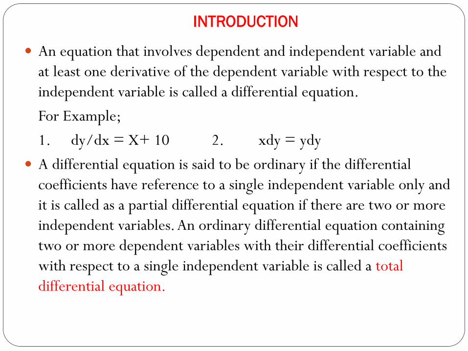
INTRODUCTION

An equation that involves dependent and independent variable and

at least one derivative of the dependent variable with respect to the

independent variable is called a differential equation.

For Example;

1. dy/dx = X+ 10 2. xdy = ydy

A differential equation is said to be ordinary if the differential

coefficients have reference to a single independent variable only and

it is called as a partial differential equation if there are two or more

independent variables. An ordinary differential equation containing

two or more dependent variables with their differential coefficients

with respect to a single independent variable is called a total

differential equation.

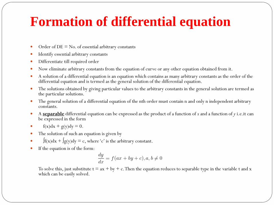
Formation of differential equation

Order of DE = No. of essential arbitrary constants

Identify essential arbitrary constants

Differentiate till required order

Now eliminate arbitrary constants from the equation of curve or any other equation obtained from it.

A solution of a differential equation is an equation which contains as many arbitrary constants as the order of the differential equation and is termed as the general solution of the differential equation.

The solutions obtained by giving particular values to the arbitrary constants in the general solution are termed as the particular solutions.

The general solution of a differential equation of the nth order must contain n and only n independent arbitrary constants.

A separable differential equation can be expressed as the product of a function of x and a function of y i.e.it can be expressed in the form

f(x)dx + g(y)dy = 0.

The solution of such an equation is given by

∫f(x)dx + ∫g(y)dy = c, where ‘c’ is the arbitrary constant.

If the equation is of the form:

To solve this, just substitute t = ax + by + c. Then the equation reduces to separable type in the variable t and x which can be easily solved.

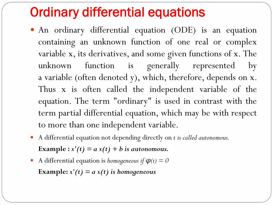
Ordinary differential equations

An ordinary differential equation (ODE) is an equation

containing an unknown function of one real or complex

variable x, its derivatives, and some given functions of x. The

unknown function is generally represented by

a variable (often denoted y), which, therefore, depends on x.

Thus x is often called the independent variable of the

equation. The term "ordinary" is used in contrast with the

term partial differential equation, which may be with respect

to more than one independent variable.

A differential equation not depending directly on t is called autonomous.

Example : x'(t) = a x(t) + b is autonomous.

A differential equation is homogeneous if φ(t) = 0

Example: x'(t) = a x(t) is homogeneous

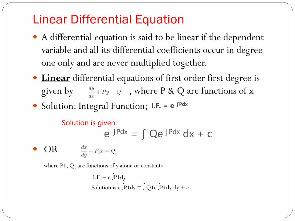
Linear Differential Equation

A differential equation is said to be linear if the dependent

variable and all its differential coefficients occur in degree

one only and are never multiplied together.

Linear differential equations of first order first degree is

given by , where P & Q are functions of x

Solution: Integral Function;

Solution is given

e ∫Pdx = ∫ Qe ∫Pdx dx + c

OR

where P1, Q1 are functions of y alone or constants

I.F. = e ∫P1dy

Solution is e ∫P1dy = ∫ Q1e ∫P1dy dy + c

I.F. = e ∫Pdx

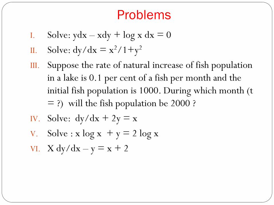
Problems

I. Solve: ydx – xdy + log x dx = 0

II. Solve: dy/dx = x2/1+y2

III. Suppose the rate of natural increase of fish population

in a lake is 0.1 per cent of a fish per month and the

initial fish population is 1000. During which month (t

= ?) will the fish population be 2000 ?

IV. Solve: dy/dx + 2y = x

V. Solve : x log x + y = 2 log x

VI. X dy/dx – y = x + 2

Solution of Ordinary Differential Equation (ODE)

A solution of an ODE is a function x(t) that satisfies the equation for all values of t. Many ODE have no solutions.

Analytic solutions -i.e., a closed expression of x in terms of t- can be found by different methods. Example: conjectures, integration.

Most ODE’s do not have analytic solutions. Numerical solutions will be needed.

If for some initial conditions a differential equation has a solution that is a constant function (independent of t), then the value of the constant, x∞, is called an equilibrium state or stationary state.

If, for all initial conditions, the solution of the differential equation converges to x∞ as t →∞, then the equilibrium is globally stable.

Classic Problem: “The rate of growth of the population is proportional to the size of the population.” Quantities: t = time, P(t) = population, k = proportionaly constant (growth-rate coefficient)

The differential equation representing this problem: dP(t)/dt = kP(t)

Note that P0=0 is a solution because dP(t)/dt = 0 forever (trivial!).

If P0 ≠ 0, how does the behavior of the model depend on P0 and k? In particular, how does it depend on the signs of P0 and k?

Guess a solution: The first derivative should be “similar” to the

function. Let’s try an exponential: P(t) = c ekt

dP(t)/dt = c k ekt = kP(t) −it works! (and, in fact, c = P0.)

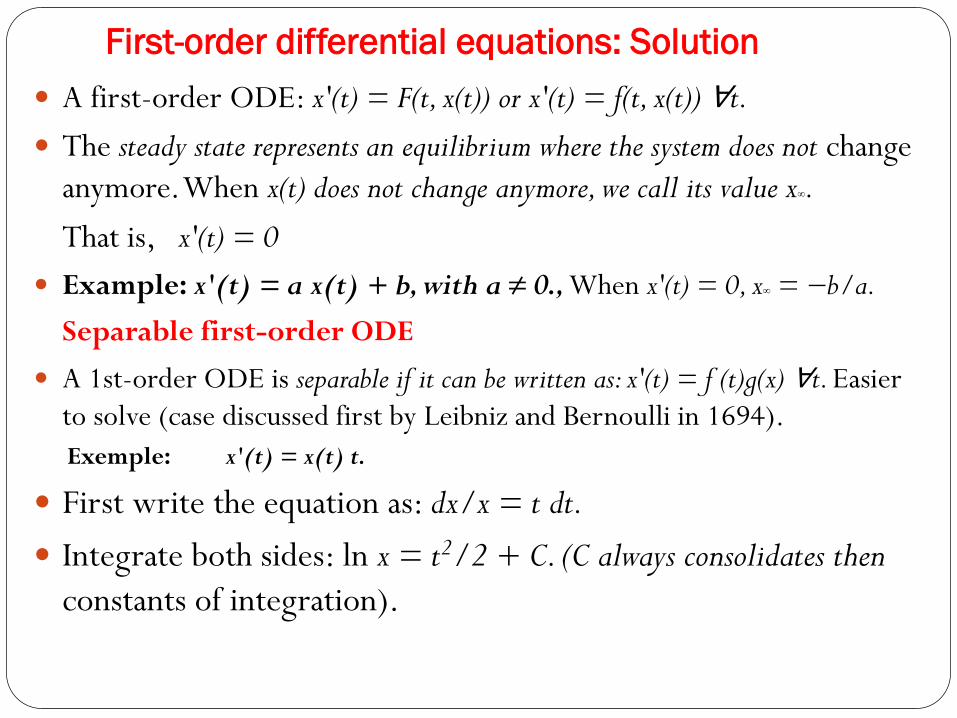
First-order differential equations: Solution

A first-order ODE: x'(t) = F(t, x(t)) or x'(t) = f(t, x(t)) ∀t.

The steady state represents an equilibrium where the system does not change

anymore. When x(t) does not change anymore, we call its value x∞.

That is, x'(t) = 0

Example: x'(t) = a x(t) + b, with a ≠ 0., When x'(t) = 0, x∞ = −b/a.

Separable first-order ODE

A 1st-order ODE is separable if it can be written as: x'(t) = f (t)g(x) ∀t. Easier

to solve (case discussed first by Leibniz and Bernoulli in 1694).

Exemple: x'(t) = x(t) t.

First write the equation as: dx/x = t dt.

Integrate both sides: ln x = t2/2 + C. (C always consolidates then

constants of integration).

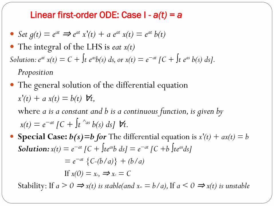
Linear first-order ODE: Case I - a(t) = a

Set g(t) = eat ⇒ eat x'(t) + a eat x(t) = eat b(t)

The integral of the LHS is eat x(t)

Solution: eat x(t) = C + ∫t easb(s) ds, or x(t) = e−at [C + ∫t eas b(s) ds].

Proposition

The general solution of the differential equation

x'(t) + a x(t) = b(t) ∀t,

where a is a constant and b is a continuous function, is given by

x(t) = e−at [C + ∫t ^as b(s) ds] ∀t.

Special Case: b(s)=b for The differential equation is x'(t) + ax(t) = b

Solution: x(t) = e−at [C + ∫teasb ds] = e−at [C +b ∫teasds]

= e−at {C-(b/a)} + (b/a)

If x(0) = x0, ⇒ x0 = C

Stability: If a > 0 ⇒ x(t) is stable(and x∞ = b/a), If a < 0 ⇒ x(t) is unstable

Linear first-order ODE: Phase Diagram

A phase diagram graphs the first-order ODE. That is, plots x’(t) and x(t).

Linear first-order ODE: Examples

Linear first-order ODE: Price Dynamics

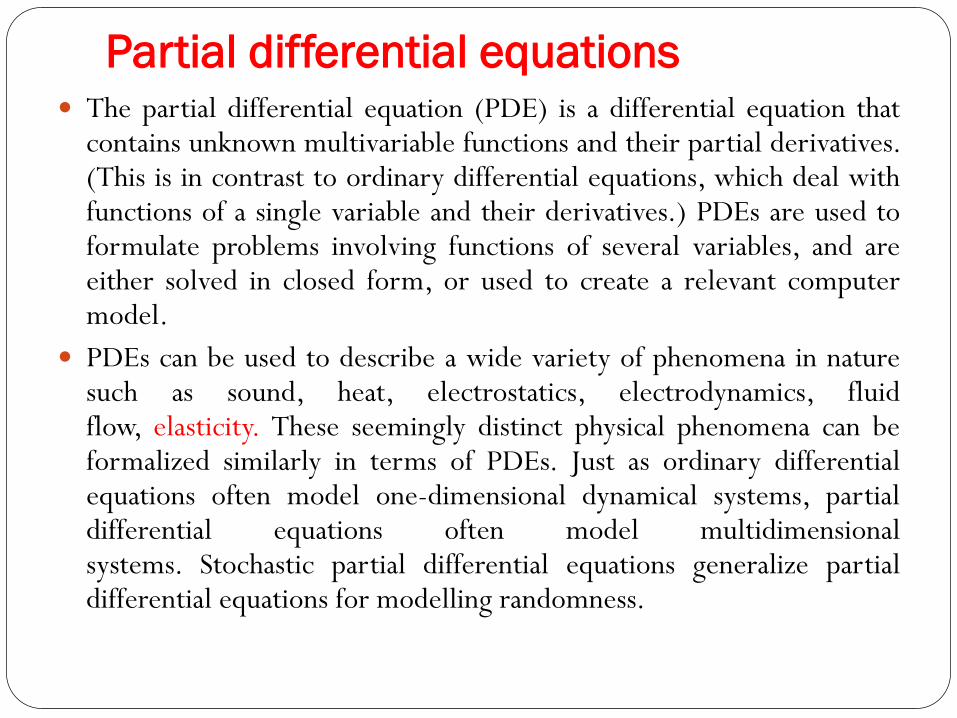
Partial differential equations The partial differential equation (PDE) is a differential equation that

contains unknown multivariable functions and their partial derivatives.(This is in contrast to ordinary differential equations, which deal withfunctions of a single variable and their derivatives.) PDEs are used toformulate problems involving functions of several variables, and areeither solved in closed form, or used to create a relevant computermodel.

PDEs can be used to describe a wide variety of phenomena in naturesuch as sound, heat, electrostatics, electrodynamics, fluidflow, elasticity. These seemingly distinct physical phenomena can beformalized similarly in terms of PDEs. Just as ordinary differentialequations often model one-dimensional dynamical systems, partialdifferential equations often model multidimensionalsystems. Stochastic partial differential equations generalize partialdifferential equations for modelling randomness.

Exact differential equation

A differential equation M(x, y)dx + N(x, y) dy = 0 is called

an exact differential equation if there exists a function u such

that du = Mdx + Ndy.

The above differential equation Mdx + Ndy = 0 is termed to

be exact if ∂M/∂y = ∂N/∂x. Its solution hence is given by

∫M dx + ∫N dy = c, where in the first integral, i.e. in M, y is

considered as a constant and in N, only those terms which are

independent of x are considered.

For Example;

Problems: Exact DE

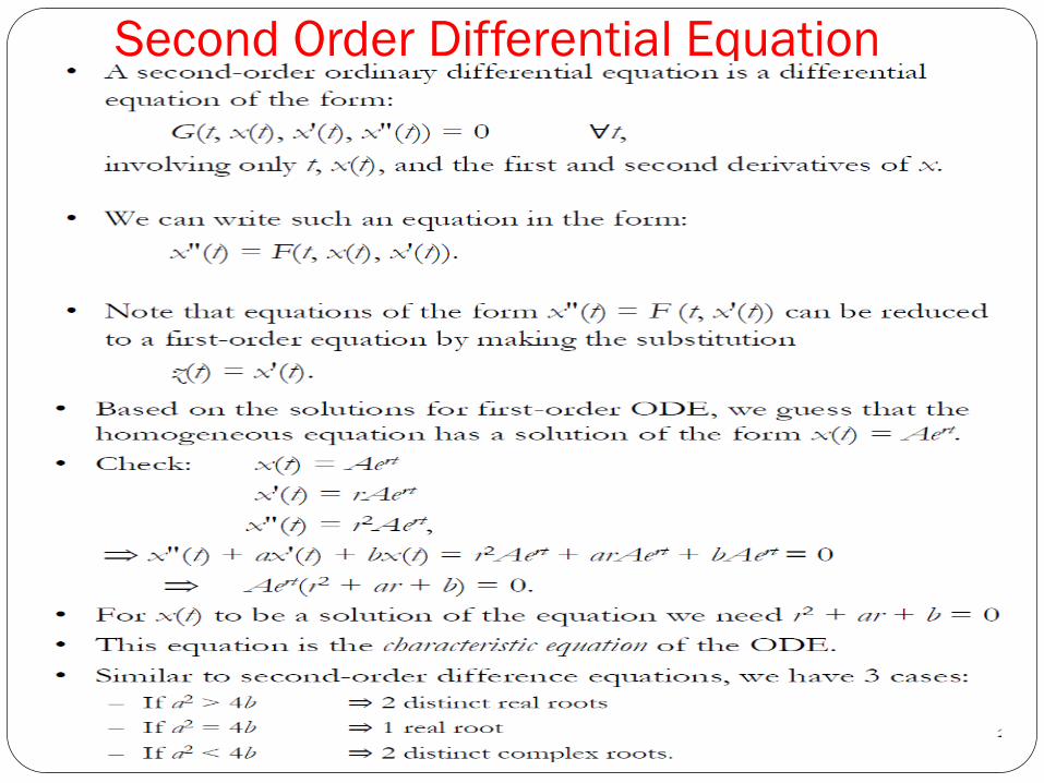
Second Order Differential Equation

Linear Second Order with Constant coefficient: Economics Example

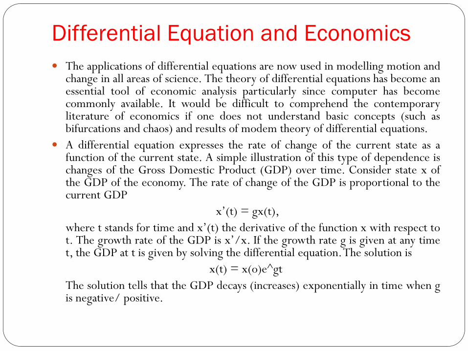
Differential Equation and Economics

The applications of differential equations are now used in modelling motion andchange in all areas of science. The theory of differential equations has become anessential tool of economic analysis particularly since computer has becomecommonly available. It would be difficult to comprehend the contemporaryliterature of economics if one does not understand basic concepts (such asbifurcations and chaos) and results of modem theory of differential equations.

A differential equation expresses the rate of change of the current state as afunction of the current state. A simple illustration of this type of dependence ischanges of the Gross Domestic Product (GDP) over time. Consider state x ofthe GDP of the economy. The rate of change of the GDP is proportional to thecurrent GDP

x’(t) = gx(t),

where t stands for time and x’(t) the derivative of the function x with respect tot. The growth rate of the GDP is x’/x. If the growth rate g is given at any timet, the GDP at t is given by solving the differential equation.The solution is

x(t) = x(o)e^gt

The solution tells that the GDP decays (increases) exponentially in time when gis negative/ positive.

Thank you