Ordinary Differential Equations - Jones & Bartlett Learning
31
PART 1 1. Introduction to Differential Equations 2. First-Order Differential Equations 3. Higher-Order Differential Equations 4. The Laplace Transform 5. Series Solutions of Linear Differential Equations 6. Numerical Solutions of Ordinary Differential Equations Ordinary Differential Equations © Nessa Gnatoush/Shutterstock © Jones & Bartlett Learning LLC, an Ascend Learning Company. NOT FOR SALE OR DISTRIBUTION.
-
Upload
khangminh22 -
Category
Documents
-
view
0 -
download
0
Transcript of Ordinary Differential Equations - Jones & Bartlett Learning
PART
11. Introduction to Differential Equations
2. First-Order Differential Equations
3. Higher-Order Differential Equations
4. The Laplace Transform
5. Series Solutions of Linear Differential Equations
6. Numerical Solutions of Ordinary Differential Equations
Ordinary Differential
Equations©
Ness
a Gn
atou
sh/S
hutt
erst
ock
58229_CH01_001_031.indd Page 1 6/6/16 2:48 PM F-0017 58229_CH01_001_031.indd Page 1 6/6/16 2:48 PM F-0017 /202/JB00127/work/indd/202/JB00127/work/indd
© Jones & Bartlett Learning LLC, an Ascend Learning Company. NOT FOR SALE OR DISTRIBUTION.
© Jones & Bartlett Learning, LLCNOT FOR SALE OR DISTRIBUTION
© Jones & Bartlett Learning, LLCNOT FOR SALE OR DISTRIBUTION
© Jones & Bartlett Learning, LLCNOT FOR SALE OR DISTRIBUTION
© Jones & Bartlett Learning, LLCNOT FOR SALE OR DISTRIBUTION
© Jones & Bartlett Learning, LLCNOT FOR SALE OR DISTRIBUTION
© Jones & Bartlett Learning, LLCNOT FOR SALE OR DISTRIBUTION
© Jones & Bartlett Learning, LLCNOT FOR SALE OR DISTRIBUTION
© Jones & Bartlett Learning, LLCNOT FOR SALE OR DISTRIBUTION
© Jones & Bartlett Learning, LLCNOT FOR SALE OR DISTRIBUTION
© Jones & Bartlett Learning, LLCNOT FOR SALE OR DISTRIBUTION
© Jones & Bartlett Learning, LLCNOT FOR SALE OR DISTRIBUTION
© Jones & Bartlett Learning, LLCNOT FOR SALE OR DISTRIBUTION
© Jones & Bartlett Learning, LLCNOT FOR SALE OR DISTRIBUTION
© Jones & Bartlett Learning, LLCNOT FOR SALE OR DISTRIBUTION
© Jones & Bartlett Learning, LLCNOT FOR SALE OR DISTRIBUTION
© Jones & Bartlett Learning, LLCNOT FOR SALE OR DISTRIBUTION
© Jones & Bartlett Learning, LLCNOT FOR SALE OR DISTRIBUTION
© Jones & Bartlett Learning, LLCNOT FOR SALE OR DISTRIBUTION
© Jones & Bartlett Learning, LLCNOT FOR SALE OR DISTRIBUTION
© Jones & Bartlett Learning, LLCNOT FOR SALE OR DISTRIBUTION

© An
dy Z
ariv
ny/S
hutt
erSt
ock,
Inc
.
58229_CH01_001_031.indd Page 2 6/6/16 2:48 PM F-0017 58229_CH01_001_031.indd Page 2 6/6/16 2:48 PM F-0017 /202/JB00127/work/indd/202/JB00127/work/indd
© Jones & Bartlett Learning LLC, an Ascend Learning Company. NOT FOR SALE OR DISTRIBUTION.
© Jones & Bartlett Learning, LLCNOT FOR SALE OR DISTRIBUTION
© Jones & Bartlett Learning, LLCNOT FOR SALE OR DISTRIBUTION
© Jones & Bartlett Learning, LLCNOT FOR SALE OR DISTRIBUTION
© Jones & Bartlett Learning, LLCNOT FOR SALE OR DISTRIBUTION
© Jones & Bartlett Learning, LLCNOT FOR SALE OR DISTRIBUTION
© Jones & Bartlett Learning, LLCNOT FOR SALE OR DISTRIBUTION
© Jones & Bartlett Learning, LLCNOT FOR SALE OR DISTRIBUTION
© Jones & Bartlett Learning, LLCNOT FOR SALE OR DISTRIBUTION
© Jones & Bartlett Learning, LLCNOT FOR SALE OR DISTRIBUTION
© Jones & Bartlett Learning, LLCNOT FOR SALE OR DISTRIBUTION
© Jones & Bartlett Learning, LLCNOT FOR SALE OR DISTRIBUTION
© Jones & Bartlett Learning, LLCNOT FOR SALE OR DISTRIBUTION
© Jones & Bartlett Learning, LLCNOT FOR SALE OR DISTRIBUTION
© Jones & Bartlett Learning, LLCNOT FOR SALE OR DISTRIBUTION
© Jones & Bartlett Learning, LLCNOT FOR SALE OR DISTRIBUTION
© Jones & Bartlett Learning, LLCNOT FOR SALE OR DISTRIBUTION
© Jones & Bartlett Learning, LLCNOT FOR SALE OR DISTRIBUTION
© Jones & Bartlett Learning, LLCNOT FOR SALE OR DISTRIBUTION
© Jones & Bartlett Learning, LLCNOT FOR SALE OR DISTRIBUTION
© Jones & Bartlett Learning, LLCNOT FOR SALE OR DISTRIBUTION
The purpose of this short chapter is twofold: to introduce the basic terminology of differential
equations and to briefly examine how differential equations arise in an attempt to describe or model physical phenomena in mathematical terms.
CHAPTER CONTENTS
1Introduction to
Differential Equations
CHAPTER
1.1 Definitions and Terminology1.2 Initial-Value Problems1.3 Differential Equations as Mathematical Models
Chapter 1 in Review
58229_CH01_001_031.indd Page 3 3/15/16 7:08 PM F-0017 58229_CH01_001_031.indd Page 3 3/15/16 7:08 PM F-0017 /202/JB00127/work/indd/202/JB00127/work/indd
© Jones & Bartlett Learning LLC, an Ascend Learning Company. NOT FOR SALE OR DISTRIBUTION.
© Jones & Bartlett Learning, LLCNOT FOR SALE OR DISTRIBUTION
© Jones & Bartlett Learning, LLCNOT FOR SALE OR DISTRIBUTION
© Jones & Bartlett Learning, LLCNOT FOR SALE OR DISTRIBUTION
© Jones & Bartlett Learning, LLCNOT FOR SALE OR DISTRIBUTION
© Jones & Bartlett Learning, LLCNOT FOR SALE OR DISTRIBUTION
© Jones & Bartlett Learning, LLCNOT FOR SALE OR DISTRIBUTION
© Jones & Bartlett Learning, LLCNOT FOR SALE OR DISTRIBUTION
© Jones & Bartlett Learning, LLCNOT FOR SALE OR DISTRIBUTION
© Jones & Bartlett Learning, LLCNOT FOR SALE OR DISTRIBUTION
© Jones & Bartlett Learning, LLCNOT FOR SALE OR DISTRIBUTION
© Jones & Bartlett Learning, LLCNOT FOR SALE OR DISTRIBUTION
© Jones & Bartlett Learning, LLCNOT FOR SALE OR DISTRIBUTION
© Jones & Bartlett Learning, LLCNOT FOR SALE OR DISTRIBUTION
© Jones & Bartlett Learning, LLCNOT FOR SALE OR DISTRIBUTION
© Jones & Bartlett Learning, LLCNOT FOR SALE OR DISTRIBUTION
© Jones & Bartlett Learning, LLCNOT FOR SALE OR DISTRIBUTION
© Jones & Bartlett Learning, LLCNOT FOR SALE OR DISTRIBUTION
© Jones & Bartlett Learning, LLCNOT FOR SALE OR DISTRIBUTION
© Jones & Bartlett Learning, LLCNOT FOR SALE OR DISTRIBUTION
© Jones & Bartlett Learning, LLCNOT FOR SALE OR DISTRIBUTION
4 | CHAPTER 1 Introduction to Differential Equations
1.1 Definitions and Terminology
INTRODUCTION The words differential and equation certainly suggest solving some kind
of equation that contains derivatives. But before you start solving anything, you must learn some
of the basic defintions and terminology of the subject.
A Definition The derivative dy/dx of a function y � f(x) is itself another function f�(x)
found by an appropriate rule. For example, the function y � e0.1x2
is differentiable on the interval
(�q , q ), and its derivative is dy/dx � 0.2xe0.1x2
. If we replace e0.1x2
in the last equation by the
symbol y, we obtain
dy
dx� 0.2xy. (1)
Now imagine that a friend of yours simply hands you the differential equation in (1), and that
you have no idea how it was constructed. Your friend asks: “What is the function represented by
the symbol y?” You are now face-to-face with one of the basic problems in a course in differen-
tial equations:
How do you solve such an equation for the unknown function y � f(x)?
The problem is loosely equivalent to the familiar reverse problem of differential calculus: Given
a derivative, find an antiderivative.
Before proceeding any further, let us give a more precise definition of the concept of a dif-
ferential equation.
In order to talk about them, we will classify a differential equation by type, order, and linearity.
Classification by Type If a differential equation contains only ordinary derivatives of
one or more functions with respect to a single independent variable it is said to be an ordinary differential equation (ODE). An equation involving only partial derivatives of one or more
functions of two or more independent variables is called a partial differential equation (PDE). Our first example illustrates several of each type of differential equation.
EXAMPLE 1 Types of Differential Equations(a) The equations
an ODE can contain more than one dependent variable
T T
dy
dx� 6y � e
�x, d 2y
dx2�
dy
dx2 12y � 0, and
dx
dt�
dy
dt� 3x � 2y (2)
are examples of ordinary differential equations.
(b) The equations
02u
0x2�02u
0y2� 0,
02u
0x2�02u
0t 220u
0t, 0u
0y� �
0v
0x (3)
are examples of partial differential equations. Notice in the third equation that there are two
dependent variables and two independent variables in the PDE. This indicates that u and v
must be functions of two or more independent variables.
Definition 1.1.1 Differential Equation
An equation containing the derivatives of one or more dependent variables, with respect to
one or more independent variables, is said to be a differential equation (DE).
58229_CH01_001_031.indd Page 4 3/15/16 7:08 PM F-0017 58229_CH01_001_031.indd Page 4 3/15/16 7:08 PM F-0017 /202/JB00127/work/indd/202/JB00127/work/indd
© Jones & Bartlett Learning LLC, an Ascend Learning Company. NOT FOR SALE OR DISTRIBUTION.
© Jones & Bartlett Learning, LLCNOT FOR SALE OR DISTRIBUTION
© Jones & Bartlett Learning, LLCNOT FOR SALE OR DISTRIBUTION
© Jones & Bartlett Learning, LLCNOT FOR SALE OR DISTRIBUTION
© Jones & Bartlett Learning, LLCNOT FOR SALE OR DISTRIBUTION
© Jones & Bartlett Learning, LLCNOT FOR SALE OR DISTRIBUTION
© Jones & Bartlett Learning, LLCNOT FOR SALE OR DISTRIBUTION
© Jones & Bartlett Learning, LLCNOT FOR SALE OR DISTRIBUTION
© Jones & Bartlett Learning, LLCNOT FOR SALE OR DISTRIBUTION
© Jones & Bartlett Learning, LLCNOT FOR SALE OR DISTRIBUTION
© Jones & Bartlett Learning, LLCNOT FOR SALE OR DISTRIBUTION
© Jones & Bartlett Learning, LLCNOT FOR SALE OR DISTRIBUTION
© Jones & Bartlett Learning, LLCNOT FOR SALE OR DISTRIBUTION
© Jones & Bartlett Learning, LLCNOT FOR SALE OR DISTRIBUTION
© Jones & Bartlett Learning, LLCNOT FOR SALE OR DISTRIBUTION
© Jones & Bartlett Learning, LLCNOT FOR SALE OR DISTRIBUTION
© Jones & Bartlett Learning, LLCNOT FOR SALE OR DISTRIBUTION
© Jones & Bartlett Learning, LLCNOT FOR SALE OR DISTRIBUTION
© Jones & Bartlett Learning, LLCNOT FOR SALE OR DISTRIBUTION
© Jones & Bartlett Learning, LLCNOT FOR SALE OR DISTRIBUTION
© Jones & Bartlett Learning, LLCNOT FOR SALE OR DISTRIBUTION
1.1 Definitions and Terminology | 5
Notation Throughout this text, ordinary derivatives will be written using either the Leibniz notation dy/dx, d 2y/dx 2, d 3y/dx 3, … , or the prime notation y�, y �, y �, … . Using the latter nota-
tion, the first two differential equations in (2) can be written a little more compactly as
y� � 6y � e�x and y � � y� � 12y � 0, respectively. Actually, the prime notation is used to denote
only the first three derivatives; the fourth derivative is written y(4) instead of y ��. In general, the
nth derivative is d ny/dx n or y(n). Although less convenient to write and to typeset, the Leibniz
notation has an advantage over the prime notation in that it clearly displays both the dependent
and independent variables. For example, in the differential equation d 2x/dt 2 � 16x � 0, it is im-
mediately seen that the symbol x now represents a dependent variable, whereas the independent
variable is t. You should also be aware that in physical sciences and engineering, Newton’s dot notation (derogatively referred to by some as the “flyspeck” notation) is sometimes used to
denote derivatives with respect to time t. Thus the differential equation d 2s/dt 2 � �32 becomes
s$ � �32. Partial derivatives are often denoted by a subscript notation indicating the indepen-
dent variables. For example, the first and second equations in (3) can be written, in turn, as
uxx � uyy � 0 and uxx � utt � ut.
Classification by Order The order of a differential equation (ODE or PDE) is the
order of the highest derivative in the equation.
EXAMPLE 2 Order of a Differential EquationThe differential equations
highest order highest order
T T
d 2y
dx 2� 5ady
dxb3
2 4y � ex, 204u
0x4�02u
0t 2� 0
are examples of a second-order ordinary differential equation and a fourth-order partial dif-
ferential equation, respectively.
A first-order ordinary differential equation is sometimes written in the differential form
M(x, y) dx � N(x, y) dy � 0.
EXAMPLE 3 Differential Form of a First-Order ODEIf we assume that y is the dependent variable in a first-order ODE, then recall from calculus
that the differential dy is defined to be dy � y9dx.
(a) By dividing by the differential dx an alternative form of the equation (y 2 x) dx 1
4x dy � 0 is given by
y 2 x � 4x
dy
dx� 0 or equivalently 4x
dy
dx� y � x.
(b) By multiplying the differential equation
6xy
dy
dx� x2 � y2 � 0
by dx we see that the equation has the alternative differential form
(x2 � y2) dx � 6xy dy � 0.
In symbols, we can express an nth-order ordinary differential equation in one dependent vari-
able by the general form
F(x, y, y�, … , y(n) ) � 0, (4)
where F is a real-valued function of n � 2 variables: x, y, y�, … , y(n). For both practical and
theoretical reasons, we shall also make the assumption hereafter that it is possible to solve an
58229_CH01_001_031.indd Page 5 5/24/16 6:50 PM f-500 58229_CH01_001_031.indd Page 5 5/24/16 6:50 PM f-500 /202/JB00127/work/indd/202/JB00127/work/indd
© Jones & Bartlett Learning LLC, an Ascend Learning Company. NOT FOR SALE OR DISTRIBUTION.
© Jones & Bartlett Learning, LLCNOT FOR SALE OR DISTRIBUTION
© Jones & Bartlett Learning, LLCNOT FOR SALE OR DISTRIBUTION
© Jones & Bartlett Learning, LLCNOT FOR SALE OR DISTRIBUTION
© Jones & Bartlett Learning, LLCNOT FOR SALE OR DISTRIBUTION
© Jones & Bartlett Learning, LLCNOT FOR SALE OR DISTRIBUTION
© Jones & Bartlett Learning, LLCNOT FOR SALE OR DISTRIBUTION
© Jones & Bartlett Learning, LLCNOT FOR SALE OR DISTRIBUTION
© Jones & Bartlett Learning, LLCNOT FOR SALE OR DISTRIBUTION
© Jones & Bartlett Learning, LLCNOT FOR SALE OR DISTRIBUTION
© Jones & Bartlett Learning, LLCNOT FOR SALE OR DISTRIBUTION
© Jones & Bartlett Learning, LLCNOT FOR SALE OR DISTRIBUTION
© Jones & Bartlett Learning, LLCNOT FOR SALE OR DISTRIBUTION
© Jones & Bartlett Learning, LLCNOT FOR SALE OR DISTRIBUTION
© Jones & Bartlett Learning, LLCNOT FOR SALE OR DISTRIBUTION
© Jones & Bartlett Learning, LLCNOT FOR SALE OR DISTRIBUTION
© Jones & Bartlett Learning, LLCNOT FOR SALE OR DISTRIBUTION
© Jones & Bartlett Learning, LLCNOT FOR SALE OR DISTRIBUTION
© Jones & Bartlett Learning, LLCNOT FOR SALE OR DISTRIBUTION
© Jones & Bartlett Learning, LLCNOT FOR SALE OR DISTRIBUTION
© Jones & Bartlett Learning, LLCNOT FOR SALE OR DISTRIBUTION
6 | CHAPTER 1 Introduction to Differential Equations
ordinary differential equation in the form (4) uniquely for the highest derivative y(n) in terms of
the remaining n � 1 variables. The differential equation
d ny
dx n � f (x, y, y9, p , y (n21) ), (5)
where f is a real-valued continuous function, is referred to as the normal form of (4). Thus, when
it suits our purposes, we shall use the normal forms
dy
dx� f (x, y) and
d 2y
dx 2� f (x, y, y9)
to represent general first- and second-order ordinary differential equations.
EXAMPLE 4 Normal Form of an ODE(a) By solving for the derivative dy/dx the normal form of the first-order differential equation
4x
dy
dx� y � x is
dy
dx�
x 2 y
4x.
(b) By solving for the derivative y0 the normal form of the second-order differential
equation
y� � y� � 6y � 0 is y� � y� � 6y.
Classification by Linearity An nth-order ordinary differential equation (4) is said to
be linear in the variable y if F is linear in y, y�, … , y(n). This means that an nth-order ODE is
linear when (4) is an(x)y (n) � an21(x)y( n21) � p � a1(x)y9 � a0(x)y 2 g(x) � 0 or
an(x) d ny
dx n � an21(x) d n21y
dxn21� p � a1(x)
dy
dx� a0(x)y � g(x). (6)
Two important special cases of (6) are linear first-order (n � 1) and linear second-order(n � 2) ODEs.
a1(x) dy
dx� a0(x)y � g(x) and a2(x)
d 2y
dx2� a1(x)
dy
dx� a0(x)y � g(x). (7)
In the additive combination on the left-hand side of (6) we see that the characteristic two proper-
ties of a linear ODE are
• The dependent variable y and all its derivatives y�, y�, … , y(n) are of the first degree; that
is, the power of each term involving y is 1.
• The coefficients a0, a1, … , an of y, y�, … , y(n) depend at most on the independent
variable x.
A nonlinear ordinary differential equation is simply one that is not linear. If the coefficients
of y, y�, … , y(n) contain the dependent variable y or its derivatives or if powers of y, y�, … ,
y(n), such as (y�)2, appear in the equation, then the DE is nonlinear. Also, nonlinear functions
of the dependent variable or its derivatives, such as sin y or ey� cannot appear in a linear
equation.
EXAMPLE 5 Linear and Nonlinear Differential Equations(a) The equations
(y 2 x) dx � 4x dy � 0, y0 2 2y9 � y � 0, x3 d 3y
dx 3
� 3x dy
dx2 5y � e
x
are, in turn, examples of linear first-, second-, and third-order ordinary differential equations.
We have just demonstrated in part (a) of Example 3 that the first equation is linear in y by
writing it in the alternative form 4xy� � y � x.
Remember these two
characteristics of a
linear ODE.
58229_CH01_001_031.indd Page 6 6/18/16 5:50 AM F-0017 58229_CH01_001_031.indd Page 6 6/18/16 5:50 AM F-0017 /202/JB00127/work/indd/202/JB00127/work/indd
© Jones & Bartlett Learning LLC, an Ascend Learning Company. NOT FOR SALE OR DISTRIBUTION.
© Jones & Bartlett Learning, LLCNOT FOR SALE OR DISTRIBUTION
© Jones & Bartlett Learning, LLCNOT FOR SALE OR DISTRIBUTION
© Jones & Bartlett Learning, LLCNOT FOR SALE OR DISTRIBUTION
© Jones & Bartlett Learning, LLCNOT FOR SALE OR DISTRIBUTION
© Jones & Bartlett Learning, LLCNOT FOR SALE OR DISTRIBUTION
© Jones & Bartlett Learning, LLCNOT FOR SALE OR DISTRIBUTION
© Jones & Bartlett Learning, LLCNOT FOR SALE OR DISTRIBUTION
© Jones & Bartlett Learning, LLCNOT FOR SALE OR DISTRIBUTION
© Jones & Bartlett Learning, LLCNOT FOR SALE OR DISTRIBUTION
© Jones & Bartlett Learning, LLCNOT FOR SALE OR DISTRIBUTION
© Jones & Bartlett Learning, LLCNOT FOR SALE OR DISTRIBUTION
© Jones & Bartlett Learning, LLCNOT FOR SALE OR DISTRIBUTION
© Jones & Bartlett Learning, LLCNOT FOR SALE OR DISTRIBUTION
© Jones & Bartlett Learning, LLCNOT FOR SALE OR DISTRIBUTION
© Jones & Bartlett Learning, LLCNOT FOR SALE OR DISTRIBUTION
© Jones & Bartlett Learning, LLCNOT FOR SALE OR DISTRIBUTION
© Jones & Bartlett Learning, LLCNOT FOR SALE OR DISTRIBUTION
© Jones & Bartlett Learning, LLCNOT FOR SALE OR DISTRIBUTION
© Jones & Bartlett Learning, LLCNOT FOR SALE OR DISTRIBUTION
© Jones & Bartlett Learning, LLCNOT FOR SALE OR DISTRIBUTION

1.1 Definitions and Terminology | 7
(b) The equations
nonlinear term: nonlinear term: nonlinear term: coefficient depends on y nonlinear function of y power not 1
T T T
(1 2 y)y9 � 2y � ex, d 2y
dx2� sin y � 0,
d 4y
dx4� y2 � 0,
are examples of nonlinear first-, second-, and fourth-order ordinary differential equations,
respectively.
Solution As stated before, one of our goals in this course is to solve—or find solutions
of—differential equations. The concept of a solution of an ordinary differential equation is
defined next.
Definition 1.1.2 Solution of an ODE
Any function f, defined on an interval I and possessing at least n derivatives that are con-
tinuous on I, which when substituted into an nth-order ordinary differential equation reduces
the equation to an identity, is said to be a solution of the equation on the interval.
In other words, a solution of an nth-order ordinary differential equation (4) is a function fthat possesses at least n derivatives and
F(x, f(x), f�(x), … , f(n)(x)) � 0 for all x in I.
We say that f satisfies the differential equation on I. For our purposes, we shall also assume that
a solution f is a real-valued function. In our initial discussion we have already seen that y � e0.1x2
is a solution of dy/dx � 0.2xy on the interval (�q , q ).
Occasionally it will be convenient to denote a solution by the alternative symbol y(x).
Interval of Definition You can’t think solution of an ordinary differential equation
without simultaneously thinking interval. The interval I in Definition 1.1.2 is variously called
the interval of definition, the interval of validity, or the domain of the solution and can be an
open interval (a, b), a closed interval [a, b], an infinite interval (a, q ), and so on.
EXAMPLE 6 Verification of a SolutionVerify that the indicated function is a solution of the given differential equation on the interval
(�q , q ).
(a) dy
dx� xy1>2; y � 1
16 x4 (b) y� � 2y� � y � 0; y � xex
SOLUTION One way of verifying that the given function is a solution is to see, after substi-
tuting, whether each side of the equation is the same for every x in the interval (�q , q ).
(a) From left-hand side: dy
dx� 4 �
x3
16�
x3
4
right-hand side: xy1>2 � x � a x4
16b1>2
� x �x2
4�
x3
4,
we see that each side of the equation is the same for every real number x. Note that y1/2 � 14x2 is,
by definition, the nonnegative square root of 116 x
4.
(b) From the derivatives y� � xex + ex and y� � xex � 2ex we have for every real number x,
left-hand side: y� � 2y� � y � (xex � 2ex) � 2(xex � ex) � xex � 0
right-hand side: 0.
Note, too, that in Example 6 each differential equation possesses the constant solution y � 0,
defined on (�q , q ). A solution of a differential equation that is identically zero on an interval
I is said to be a trivial solution.
58229_CH01_001_031.indd Page 7 3/15/16 7:09 PM F-0017 58229_CH01_001_031.indd Page 7 3/15/16 7:09 PM F-0017 /202/JB00127/work/indd/202/JB00127/work/indd
© Jones & Bartlett Learning LLC, an Ascend Learning Company. NOT FOR SALE OR DISTRIBUTION.
© Jones & Bartlett Learning, LLCNOT FOR SALE OR DISTRIBUTION
© Jones & Bartlett Learning, LLCNOT FOR SALE OR DISTRIBUTION
© Jones & Bartlett Learning, LLCNOT FOR SALE OR DISTRIBUTION
© Jones & Bartlett Learning, LLCNOT FOR SALE OR DISTRIBUTION
© Jones & Bartlett Learning, LLCNOT FOR SALE OR DISTRIBUTION
© Jones & Bartlett Learning, LLCNOT FOR SALE OR DISTRIBUTION
© Jones & Bartlett Learning, LLCNOT FOR SALE OR DISTRIBUTION
© Jones & Bartlett Learning, LLCNOT FOR SALE OR DISTRIBUTION
© Jones & Bartlett Learning, LLCNOT FOR SALE OR DISTRIBUTION
© Jones & Bartlett Learning, LLCNOT FOR SALE OR DISTRIBUTION
© Jones & Bartlett Learning, LLCNOT FOR SALE OR DISTRIBUTION
© Jones & Bartlett Learning, LLCNOT FOR SALE OR DISTRIBUTION
© Jones & Bartlett Learning, LLCNOT FOR SALE OR DISTRIBUTION
© Jones & Bartlett Learning, LLCNOT FOR SALE OR DISTRIBUTION
© Jones & Bartlett Learning, LLCNOT FOR SALE OR DISTRIBUTION
© Jones & Bartlett Learning, LLCNOT FOR SALE OR DISTRIBUTION
© Jones & Bartlett Learning, LLCNOT FOR SALE OR DISTRIBUTION
© Jones & Bartlett Learning, LLCNOT FOR SALE OR DISTRIBUTION
© Jones & Bartlett Learning, LLCNOT FOR SALE OR DISTRIBUTION
© Jones & Bartlett Learning, LLCNOT FOR SALE OR DISTRIBUTION
8 | CHAPTER 1 Introduction to Differential Equations
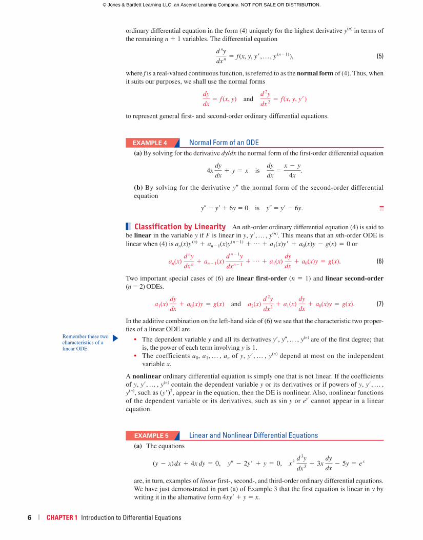
Solution Curve The graph of a solution f of an ODE is called a solution curve. Since
f is a differentiable function, it is continuous on its interval I of definition. Thus there may be a
difference between the graph of the function f and the graph of the solution f. Put another way,
the domain of the function f does not need to be the same as the interval I of definition (or
domain) of the solution f.
EXAMPLE 7 Function vs. Solution(a) Considered simply as a function, the domain of y � 1/x is the set of all real numbers xexcept 0. When we graph y � 1/x, we plot points in the xy-plane corresponding to a judicious
sampling of numbers taken from its domain. The rational function y � 1/x is discontinuous
at 0, and its graph, in a neighborhood of the origin, is given in FIGURE 1.1.1(a). The function
y � 1/x is not differentiable at x � 0 since the y-axis (whose equation is x � 0) is a vertical
asymptote of the graph.
(b) Now y � 1/x is also a solution of the linear first-order differential equation xy� � y � 0
(verify). But when we say y � 1/x is a solution of this DE we mean it is a function defined on
an interval I on which it is differentiable and satisfies the equation. In other words,
y � 1/x is a solution of the DE on any interval not containing 0, such as (�3, �1), ( 12, 10),
(�q, 0), or (0, q). Because the solution curves defined by y � 1/x on the intervals (�3, �1)
and on (12, 10) are simply segments or pieces of the solution curves defined by
y � 1/x on (�q, 0) and (0, q), respectively, it makes sense to take the interval I to be as large
as possible. Thus we would take I to be either (�q, 0) or (0, q). The solution curve on the
interval (0, q) is shown in Figure 1.1.1(b).
Explicit and Implicit Solutions You should be familiar with the terms explicit and
implicit functions from your study of calculus. A solution in which the dependent variable is
expressed solely in terms of the independent variable and constants is said to be an explicit solution.
For our purposes, let us think of an explicit solution as an explicit formula y � f(x) that we can
manipulate, evaluate, and differentiate using the standard rules. We have just seen in the last two
examples that y � 116 x 4, y � xex, and y � 1/x are, in turn, explicit solutions of dy/dx � xy1/2,
y � � 2y� � y � 0, and xy� � y � 0. Moreover, the trivial solution y � 0 is an explicit solution
of all three equations. We shall see when we get down to the business of actually solving some
ordinary differential equations that methods of solution do not always lead directly to an explicit
solution y � f(x). This is particularly true when attempting to solve nonlinear first-order dif-
ferential equations. Often we have to be content with a relation or expression G(x, y) � 0 that
defines a solution f implicitly.
Definition 1.1.3 Implicit Solution of an ODE
A relation G(x, y) � 0 is said to be an implicit solution of an ordinary differential equation (4)
on an interval I provided there exists at least one function f that satisfies the relation as well
as the differential equation on I.
It is beyond the scope of this course to investigate the conditions under which a relation
G(x, y) � 0 defines a differentiable function f. So we shall assume that if the formal implementa-
tion of a method of solution leads to a relation G(x, y) � 0, then there exists at least one function
f that satisfies both the relation (that is, G(x, f(x)) � 0) and the differential equation on an in-
terval I. If the implicit solution G(x, y) � 0 is fairly simple, we may be able to solve for y in terms
of x and obtain one or more explicit solutions. See (iv) in the Remarks.
EXAMPLE 8 Verification of an Implicit SolutionThe relation x2 � y2 � 25 is an implicit solution of the nonlinear differential equation
dy
dx� �
xy
(8)
y
x1
1
y
x1
1
(a) Function y = 1/x, x ≠ 0
(b) Solution y = 1/x, (0, ∞)
FIGURE 1.1.1 Example 7 illustrates
the difference between the function
y � 1/x and the solution y � 1/x
58229_CH01_001_031.indd Page 8 3/15/16 7:09 PM F-0017 58229_CH01_001_031.indd Page 8 3/15/16 7:09 PM F-0017 /202/JB00127/work/indd/202/JB00127/work/indd
© Jones & Bartlett Learning LLC, an Ascend Learning Company. NOT FOR SALE OR DISTRIBUTION.
© Jones & Bartlett Learning, LLCNOT FOR SALE OR DISTRIBUTION
© Jones & Bartlett Learning, LLCNOT FOR SALE OR DISTRIBUTION
© Jones & Bartlett Learning, LLCNOT FOR SALE OR DISTRIBUTION
© Jones & Bartlett Learning, LLCNOT FOR SALE OR DISTRIBUTION
© Jones & Bartlett Learning, LLCNOT FOR SALE OR DISTRIBUTION
© Jones & Bartlett Learning, LLCNOT FOR SALE OR DISTRIBUTION
© Jones & Bartlett Learning, LLCNOT FOR SALE OR DISTRIBUTION
© Jones & Bartlett Learning, LLCNOT FOR SALE OR DISTRIBUTION
© Jones & Bartlett Learning, LLCNOT FOR SALE OR DISTRIBUTION
© Jones & Bartlett Learning, LLCNOT FOR SALE OR DISTRIBUTION
© Jones & Bartlett Learning, LLCNOT FOR SALE OR DISTRIBUTION
© Jones & Bartlett Learning, LLCNOT FOR SALE OR DISTRIBUTION
© Jones & Bartlett Learning, LLCNOT FOR SALE OR DISTRIBUTION
© Jones & Bartlett Learning, LLCNOT FOR SALE OR DISTRIBUTION
© Jones & Bartlett Learning, LLCNOT FOR SALE OR DISTRIBUTION
© Jones & Bartlett Learning, LLCNOT FOR SALE OR DISTRIBUTION
© Jones & Bartlett Learning, LLCNOT FOR SALE OR DISTRIBUTION
© Jones & Bartlett Learning, LLCNOT FOR SALE OR DISTRIBUTION
© Jones & Bartlett Learning, LLCNOT FOR SALE OR DISTRIBUTION
© Jones & Bartlett Learning, LLCNOT FOR SALE OR DISTRIBUTION
1.1 Definitions and Terminology | 9
on the interval defined by �5 x 5. By implicit differentiation we obtain
d
dx x 2 �
d
dx y2 �
d
dx 25 or 2x � 2y
dy
dx� 0. (9)
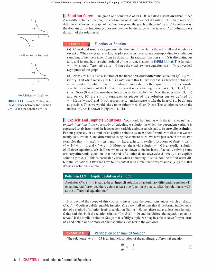
Solving the last equation in (9) for the symbol dy/dx gives (8). Moreover, solving x2 � y2 � 25
for y in terms of x yields y � "25 2 x2. The two functions y � f1(x) � "25 2 x2 and
y � f2(x) � �"25 2 x2 satisfy the relation (that is, x2 � f21 � 25 and x2 � f2
2 � 25) and are
explicit solutions defined on the interval (�5, 5). The solution curves given in FIGURE 1.1.2(b) and 1.1.2(c) are segments of the graph of the implicit solution in Figure 1.1.2(a).
x
y
c > 0
c = 0c < 0
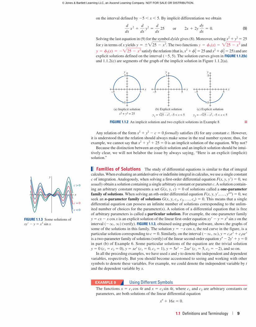
FIGURE 1.1.3 Some solutions of
xy� � y � x 2 sin x
Any relation of the form x2 � y2 � c � 0 formally satisfies (8) for any constant c. However,
it is understood that the relation should always make sense in the real number system; thus, for
example, we cannot say that x2 � y2 � 25 � 0 is an implicit solution of the equation. Why not?
Because the distinction between an explicit solution and an implicit solution should be intui-
tively clear, we will not belabor the issue by always saying, “Here is an explicit (implicit)
solution.”
Families of Solutions The study of differential equations is similar to that of integral
calculus. When evaluating an antiderivative or indefinite integral in calculus, we use a single constant
c of integration. Analogously, when solving a first-order differential equation F(x, y, y�) � 0, we
usually obtain a solution containing a single arbitrary constant or parameter c. A solution contain-
ing an arbitrary constant represents a set G(x, y, c) � 0 of solutions called a one-parameter family of solutions. When solving an nth-order differential equation F(x, y, y�, … , y(n)) � 0, we
seek an n-parameter family of solutions G(x, y, c1, c2, … , cn) � 0. This means that a single
differential equation can possess an infinite number of solutions corresponding to the unlim-
ited number of choices for the parameter(s). A solution of a differential equation that is free
of arbitrary parameters is called a particular solution. For example, the one-parameter family
y � cx � x cos x is an explicit solution of the linear first-order equation xy� � y � x2 sin x on the
interval (�q , q ) (verify). FIGURE 1.1.3, obtained using graphing software, shows the graphs of
some of the solutions in this family. The solution y � �x cos x, the red curve in the figure, is a
particular solution corresponding to c � 0. Similarly, on the interval (�q , q ), y � c1e x � c2xe x is a two-parameter family of solutions (verify) of the linear second-order equation y � � 2y� � y � 0
in part (b) of Example 6. Some particular solutions of the equation are the trivial solution
y � 0 (c1 � c2 � 0), y � xex (c1 � 0, c2 � 1), y � 5e x � 2xe x (c1 � 5, c2 � �2), and so on.
In all the preceding examples, we have used x and y to denote the independent and dependent
variables, respectively. But you should become accustomed to seeing and working with other
symbols to denote these variables. For example, we could denote the independent variable by t and the dependent variable by x.
EXAMPLE 9 Using Different SymbolsThe functions x � c1 cos 4t and x � c2 sin 4t, where c1 and c2 are arbitrary constants or
parameters, are both solutions of the linear differential equation
x� � 16x � 0.
(a) Implicit solution
5
–5
x
y
–5
5
x2 + y2 = 25(b) Explicit solution
y1 = √25 – x2, –5 < x < 5
5x
y
–5
5
(c) Explicit solution
y2 = –√25 – x2, –5 < x < 5
5
–5
x
y
–5
5
FIGURE 1.1.2 An implicit solution and two explicit solutions in Example 8
58229_CH01_001_031.indd Page 9 3/15/16 7:09 PM F-0017 58229_CH01_001_031.indd Page 9 3/15/16 7:09 PM F-0017 /202/JB00127/work/indd/202/JB00127/work/indd
© Jones & Bartlett Learning LLC, an Ascend Learning Company. NOT FOR SALE OR DISTRIBUTION.
© Jones & Bartlett Learning, LLCNOT FOR SALE OR DISTRIBUTION
© Jones & Bartlett Learning, LLCNOT FOR SALE OR DISTRIBUTION
© Jones & Bartlett Learning, LLCNOT FOR SALE OR DISTRIBUTION
© Jones & Bartlett Learning, LLCNOT FOR SALE OR DISTRIBUTION
© Jones & Bartlett Learning, LLCNOT FOR SALE OR DISTRIBUTION
© Jones & Bartlett Learning, LLCNOT FOR SALE OR DISTRIBUTION
© Jones & Bartlett Learning, LLCNOT FOR SALE OR DISTRIBUTION
© Jones & Bartlett Learning, LLCNOT FOR SALE OR DISTRIBUTION
© Jones & Bartlett Learning, LLCNOT FOR SALE OR DISTRIBUTION
© Jones & Bartlett Learning, LLCNOT FOR SALE OR DISTRIBUTION
© Jones & Bartlett Learning, LLCNOT FOR SALE OR DISTRIBUTION
© Jones & Bartlett Learning, LLCNOT FOR SALE OR DISTRIBUTION
© Jones & Bartlett Learning, LLCNOT FOR SALE OR DISTRIBUTION
© Jones & Bartlett Learning, LLCNOT FOR SALE OR DISTRIBUTION
© Jones & Bartlett Learning, LLCNOT FOR SALE OR DISTRIBUTION
© Jones & Bartlett Learning, LLCNOT FOR SALE OR DISTRIBUTION
© Jones & Bartlett Learning, LLCNOT FOR SALE OR DISTRIBUTION
© Jones & Bartlett Learning, LLCNOT FOR SALE OR DISTRIBUTION
© Jones & Bartlett Learning, LLCNOT FOR SALE OR DISTRIBUTION
© Jones & Bartlett Learning, LLCNOT FOR SALE OR DISTRIBUTION
10 | CHAPTER 1 Introduction to Differential Equations
For x � c1 cos 4t, the first two derivatives with respect to t are x� � �4c1 sin 4t and
x� � �16c1 cos 4t. Substituting x� and x then gives
x� � 16x � �16c1 cos 4t � 16(c1 cos 4t) � 0.
In like manner, for x � c2 sin 4t we have x� � �16c2 sin 4t, and so
x� � 16x � �16c2 sin 4t � 16(c2 sin 4t) � 0.
Finally, it is straightforward to verify that the linear combination of solutions for the two-
parameter family x � c1 cos 4t � c2 sin 4t is also a solution of the differential equation.
The next example shows that a solution of a differential equation can be a piecewise-defined
function.
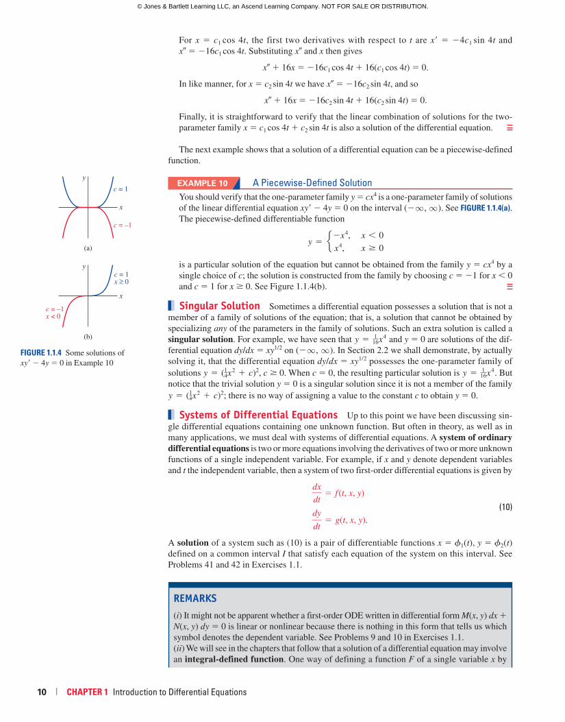
EXAMPLE 10 A Piecewise-Defined SolutionYou should verify that the one-parameter family y � cx4 is a one-parameter family of solutions
of the linear differential equation xy� � 4y � 0 on the interval (�q , q ). See FIGURE 1.1.4(a). The piecewise-defined differentiable function
y � e�x4, x , 0
x4, x $ 0
is a particular solution of the equation but cannot be obtained from the family y � cx4 by a
single choice of c; the solution is constructed from the family by choosing c � �1 for x 0
and c � 1 for x � 0. See Figure 1.1.4(b).
Singular Solution Sometimes a differential equation possesses a solution that is not a
member of a family of solutions of the equation; that is, a solution that cannot be obtained by
specializing any of the parameters in the family of solutions. Such an extra solution is called a
singular solution. For example, we have seen that y � 116x
4 and y � 0 are solutions of the dif-
ferential equation dy/dx � xy1/2 on (�q , q ). In Section 2.2 we shall demonstrate, by actually
solving it, that the differential equation dy/dx � xy1/2 possesses the one-parameter family of
solutions y � (14x
2 � c)2, c � 0. When c � 0, the resulting particular solution is y � 116x
4. But
notice that the trivial solution y � 0 is a singular solution since it is not a member of the family
y � (14x
2 � c)2; there is no way of assigning a value to the constant c to obtain y � 0.
Systems of Differential Equations Up to this point we have been discussing sin-
gle differential equations containing one unknown function. But often in theory, as well as in
many applications, we must deal with systems of differential equations. A system of ordinary differential equations is two or more equations involving the derivatives of two or more unknown
functions of a single independent variable. For example, if x and y denote dependent variables
and t the independent variable, then a system of two first-order differential equations is given by
dx
dt� f (t, x, y)
dy
dt� g(t, x, y).
(10)
A solution of a system such as (10) is a pair of differentiable functions x � f1(t), y � f2(t) defined on a common interval I that satisfy each equation of the system on this interval. See
Problems 41 and 42 in Exercises 1.1.
(a)
x
yc = 1
c = –1
c = 1x ≥ 0
c = –1x < 0
(b)
x
y
FIGURE 1.1.4 Some solutions of
xy� � 4y � 0 in Example 10
REMARKS
(i) It might not be apparent whether a first-order ODE written in differential form M(x, y) dx �N(x, y) dy � 0 is linear or nonlinear because there is nothing in this form that tells us which
symbol denotes the dependent variable. See Problems 9 and 10 in Exercises 1.1.
(ii) We will see in the chapters that follow that a solution of a differential equation may involve
an integral-defined function. One way of defining a function F of a single variable x by
58229_CH01_001_031.indd Page 10 3/15/16 7:09 PM F-0017 58229_CH01_001_031.indd Page 10 3/15/16 7:09 PM F-0017 /202/JB00127/work/indd/202/JB00127/work/indd
© Jones & Bartlett Learning LLC, an Ascend Learning Company. NOT FOR SALE OR DISTRIBUTION.
© Jones & Bartlett Learning, LLCNOT FOR SALE OR DISTRIBUTION
© Jones & Bartlett Learning, LLCNOT FOR SALE OR DISTRIBUTION
© Jones & Bartlett Learning, LLCNOT FOR SALE OR DISTRIBUTION
© Jones & Bartlett Learning, LLCNOT FOR SALE OR DISTRIBUTION
© Jones & Bartlett Learning, LLCNOT FOR SALE OR DISTRIBUTION
© Jones & Bartlett Learning, LLCNOT FOR SALE OR DISTRIBUTION
© Jones & Bartlett Learning, LLCNOT FOR SALE OR DISTRIBUTION
© Jones & Bartlett Learning, LLCNOT FOR SALE OR DISTRIBUTION
© Jones & Bartlett Learning, LLCNOT FOR SALE OR DISTRIBUTION
© Jones & Bartlett Learning, LLCNOT FOR SALE OR DISTRIBUTION
© Jones & Bartlett Learning, LLCNOT FOR SALE OR DISTRIBUTION
© Jones & Bartlett Learning, LLCNOT FOR SALE OR DISTRIBUTION
© Jones & Bartlett Learning, LLCNOT FOR SALE OR DISTRIBUTION
© Jones & Bartlett Learning, LLCNOT FOR SALE OR DISTRIBUTION
© Jones & Bartlett Learning, LLCNOT FOR SALE OR DISTRIBUTION
© Jones & Bartlett Learning, LLCNOT FOR SALE OR DISTRIBUTION
© Jones & Bartlett Learning, LLCNOT FOR SALE OR DISTRIBUTION
© Jones & Bartlett Learning, LLCNOT FOR SALE OR DISTRIBUTION
© Jones & Bartlett Learning, LLCNOT FOR SALE OR DISTRIBUTION
© Jones & Bartlett Learning, LLCNOT FOR SALE OR DISTRIBUTION
1.1 Definitions and Terminology | 11
means of a definite integral is
F(x) � #x
a
g(t) dt. (11)
If the integrand g in (11) is continuous on an interval [a, b] and a � x � b, then the derivative
form of the Fundamental Theorem of Calculus states that F is differentiable on (a, b) and
F9(x) �d
dx#x
a
g(t) dt � g(x). (12)
The integral in (11) is often nonelementary, that is, an integral of a function g that does
not have an elementary-function antiderivative. Elementary functions include the familiar
functions studied in a typical precalculus course:
constant, polynomial, rational, exponential, logarithmic, trigonometric, and inverse trigonometric functions,
as well as rational powers of these functions, finite combinations of these functions using
addition, subtraction, multiplication, division, and function compositions. For example, even
though e�t 2
, "1 � t 3, and cos t2 are elementary functions, the integrals ee�t 2
dt, e"1 � t 3 dt, and ecos t
2 dt are nonelementary. See Problems 25–28 in Exercises 1.1.
(iii) Although the concept of a solution of a differential equation has been emphasized in this
section, you should be aware that a DE does not necessarily have to possess a solution. See
Problem 43 in Exercises 1.1. The question of whether a solution exists will be touched on in
the next section.
(iv) A few last words about implicit solutions of differential equations are in order. In Example 8
we were able to solve the relation x2 � y2 � 25 for y in terms of x to get two explicit solutions,
f1(x) � "25 2 x2 and f2(x) � �"25 2 x2, of the differential equation (8). But don’t
read too much into this one example. Unless it is easy, obvious, or important, or you are in-
structed to, there is usually no need to try to solve an implicit solution G(x, y) � 0 for y ex-
plicitly in terms of x. Also do not misinterpret the second sentence following Definition 1.1.3.
An implicit solution G(x, y) � 0 can define a perfectly good differentiable function f that is
a solution of a DE, but yet we may not be able to solve G(x, y) � 0 using analytical methods
such as algebra. The solution curve of f may be a segment or piece of the graph of G(x, y) � 0.
See Problems 49 and 50 in Exercises 1.1.
(v) If every solution of an nth-order ODE F(x, y, y�, … , y(n)) � 0 on an interval I can be obtained
from an n-parameter family G(x, y, c1, c2, … , cn) � 0 by appropriate choices of the parameters
ci, i � 1, 2, … , n, we then say that the family is the general solution of the DE. In solving
linear ODEs, we shall impose relatively simple restrictions on the coefficients of the equation;
with these restrictions one can be assured that not only does a solution exist on an interval but
also that a family of solutions yields all possible solutions. Nonlinear equations, with the
exception of some first-order DEs, are usually difficult or even impossible to solve in terms
of familiar elementary functions. Furthermore, if we happen to obtain a family of solutions
for a nonlinear equation, it is not evident whether this family contains all solutions. On a
practical level, then, the designation “general solution” is applied only to linear DEs. Don’t
be concerned about this concept at this point but store the words general solution in the back
of your mind—we will come back to this notion in Section 2.3 and again in Chapter 3.
In Problems 1–8, state the order of the given ordinary
differential equation. Determine whether the equation is linear
or nonlinear by matching it with (6).
1. (1 � x)y� � 4xy� � 5y � cos x
2. x
d 3y
dx32 ady
dxb4
� y � 0
3. t 5y(4) � t 3y� � 6y � 0
4. d 2u
dr 2�
du
dr� u � cos (r � u)
5. d 2y
dx 2� Å1 � ady
dxb2
Exercises Answers to selected odd-numbered problems begin on page ANS-1.1.1
58229_CH01_001_031.indd Page 11 6/28/16 11:17 PM F-0017 58229_CH01_001_031.indd Page 11 6/28/16 11:17 PM F-0017 /202/JB00127/work/indd/202/JB00127/work/indd
© Jones & Bartlett Learning LLC, an Ascend Learning Company. NOT FOR SALE OR DISTRIBUTION.
© Jones & Bartlett Learning, LLCNOT FOR SALE OR DISTRIBUTION
© Jones & Bartlett Learning, LLCNOT FOR SALE OR DISTRIBUTION
© Jones & Bartlett Learning, LLCNOT FOR SALE OR DISTRIBUTION
© Jones & Bartlett Learning, LLCNOT FOR SALE OR DISTRIBUTION
© Jones & Bartlett Learning, LLCNOT FOR SALE OR DISTRIBUTION
© Jones & Bartlett Learning, LLCNOT FOR SALE OR DISTRIBUTION
© Jones & Bartlett Learning, LLCNOT FOR SALE OR DISTRIBUTION
© Jones & Bartlett Learning, LLCNOT FOR SALE OR DISTRIBUTION
© Jones & Bartlett Learning, LLCNOT FOR SALE OR DISTRIBUTION
© Jones & Bartlett Learning, LLCNOT FOR SALE OR DISTRIBUTION
© Jones & Bartlett Learning, LLCNOT FOR SALE OR DISTRIBUTION
© Jones & Bartlett Learning, LLCNOT FOR SALE OR DISTRIBUTION
© Jones & Bartlett Learning, LLCNOT FOR SALE OR DISTRIBUTION
© Jones & Bartlett Learning, LLCNOT FOR SALE OR DISTRIBUTION
© Jones & Bartlett Learning, LLCNOT FOR SALE OR DISTRIBUTION
© Jones & Bartlett Learning, LLCNOT FOR SALE OR DISTRIBUTION
© Jones & Bartlett Learning, LLCNOT FOR SALE OR DISTRIBUTION
© Jones & Bartlett Learning, LLCNOT FOR SALE OR DISTRIBUTION
© Jones & Bartlett Learning, LLCNOT FOR SALE OR DISTRIBUTION
© Jones & Bartlett Learning, LLCNOT FOR SALE OR DISTRIBUTION
12 | CHAPTER 1 Introduction to Differential Equations
6. d 2R
dt 2� �
k
R2
7. (sin u)y � � (cos u)y� � 2
8. x$ 2 (1 2 13x#
2 ) x# � x � 0
In Problems 9 and 10, determine whether the given first-order
differential equation is linear in the indicated dependent
variable by matching it with the first differential equation
given in (7).
9. ( y2 � 1) dx � x dy � 0; in y; in x
10. u dv � (v � uv � ueu) du � 0; in v; in u
In Problems 11–14, verify that the indicated function is an
explicit solution of the given differential equation. Assume
an appropriate interval I of definition for each solution.
11. 2y� � y � 0; y � e�x/2
12. dy
dt� 20y � 24; y � 6
5 2 65 e�20t
13. y� � 6y� � 13y � 0; y � e3x cos 2x
14. y� � y � tan x; y � �(cos x) ln(sec x � tan x)
In Problems 15–18, verify that the indicated function y � f(x)
is an explicit solution of the given first-order differential
equation. Proceed as in Example 7, by considering f simply
as a function, give its domain. Then by considering f as a
solution of the differential equation, give at least one interval I of definition.
15. (y 2 x)y9 � y 2 x � 8; y � x � 4"x � 2
16. y� � 25 � y2; y � 5 tan 5x
17. y� � 2xy2; y � 1/(4 � x2)
18. 2y� � y3 cos x; y � (1 � sin x)�1/2
In Problems 19 and 20, verify that the indicated expression is
an implicit solution of the given first-order differential equation.
Find at least one explicit solution y � f(x) in each case. Use a
graphing utility to obtain the graph of an explicit solution.
Give an interval I of definition of each solution f.
19. dX
dt� (X 2 1)(1 2 2X); lna2X 2 1
X 2 1b � t
20. 2xy dx � (x2 � y) dy � 0; �2x2y � y2 � 1
In Problems 21–24, verify that the indicated family of functions
is a solution of the given differential equation. Assume an
appropriate interval I of definition for each solution.
21. dP
dt� P(1 2 P); P �
c1et
1 � c1et
22. dy
dx� 4xy � 8x3; y � 2x2 2 1 � c1e
�2x2
23. d 2y
dx 22 4
dy
dx� 4y � 0; y � c1e
2x � c2xe2x
24. x3 d 3y
dx 3� 2x2
d 2y
dx 22 x
dy
dx� y � 12x 2;
y � c1x�1 � c2x � c3x ln x � 4x2
In Problems 25–28, use (12) to verify that the indicated function
is a solution of the given differential equation. Assume an
appropriate interval I of definition of each solution.
25. x
dy
dx2 3xy � 1; y � e3x#
x
1
e�3t
t dt
26. 2x
dy
dx2 y � 2x cos x; y � "x#
x
4
cos t"t dt
27. x2
dy
dx� xy � 10 sin x; y �
5
x�
10
x #x
1
sin t
t dt
28. dy
dx� 2xy � 1; y � e�x2
� e�x2#x
0
et 2
dt
29. Verify that the piecewise-defined function
y � e�x 2, x , 0
x 2, x $ 0
is a solution of the differential equation xy� � 2y � 0 on the
interval (�q , q ).
30. In Example 8 we saw that y � f1(x) � "25 2 x 2 and
y � f2(x) � �"25 2 x 2 are solutions of dy/dx � �x/y
on the interval (�5, 5). Explain why the piecewise-defined
function
y � e "25 2 x 2, �5 , x , 0
�"25 2 x 2, 0 # x , 5
is not a solution of the differential equation on the interval
(�5, 5).
In Problems 31–34, find values of m so that the function y � emx
is a solution of the given differential equation.
31. y� � 2y � 0 32. 3y� � 4y
33. y� � 5y� � 6y � 0 34. 2y� � 9y� � 5y � 0
In Problems 35 and 36, find values of m so that the function
y � xm is a solution of the given differential equation.
35. xy� � 2y� � 0 36. x2y� � 7xy� � 15y � 0
In Problems 37–40, use the concept that y � c, �q x q ,
is a constant function if and only if y� � 0 to determine whether
the given differential equation possesses constant solutions.
37. 3xy� � 5y � 10 38. y� � y2 � 2y � 3
39. ( y � 1)y� � 1 40. y� � 4y� � 6y � 10
In Problems 41 and 42, verify that the indicated pair of functions
is a solution of the given system of differential equations on the
interval (�q , q ).
41. dx
dt� x � 3y 42.
d 2x
dt2� 4y � et
dy
dt� 5x � 3y;
d 2y
dt 2� 4x 2 et;
x � e�2t � 3e6t, x � cos 2t � sin 2t � 15 et,
y � �e�2t � 5e6t y � �cos 2t � sin 2t � 15 et
58229_CH01_001_031.indd Page 12 5/24/16 6:50 PM f-500 58229_CH01_001_031.indd Page 12 5/24/16 6:50 PM f-500 /202/JB00127/work/indd/202/JB00127/work/indd
© Jones & Bartlett Learning LLC, an Ascend Learning Company. NOT FOR SALE OR DISTRIBUTION.
© Jones & Bartlett Learning, LLCNOT FOR SALE OR DISTRIBUTION
© Jones & Bartlett Learning, LLCNOT FOR SALE OR DISTRIBUTION
© Jones & Bartlett Learning, LLCNOT FOR SALE OR DISTRIBUTION
© Jones & Bartlett Learning, LLCNOT FOR SALE OR DISTRIBUTION
© Jones & Bartlett Learning, LLCNOT FOR SALE OR DISTRIBUTION
© Jones & Bartlett Learning, LLCNOT FOR SALE OR DISTRIBUTION
© Jones & Bartlett Learning, LLCNOT FOR SALE OR DISTRIBUTION
© Jones & Bartlett Learning, LLCNOT FOR SALE OR DISTRIBUTION
© Jones & Bartlett Learning, LLCNOT FOR SALE OR DISTRIBUTION
© Jones & Bartlett Learning, LLCNOT FOR SALE OR DISTRIBUTION
© Jones & Bartlett Learning, LLCNOT FOR SALE OR DISTRIBUTION
© Jones & Bartlett Learning, LLCNOT FOR SALE OR DISTRIBUTION
© Jones & Bartlett Learning, LLCNOT FOR SALE OR DISTRIBUTION
© Jones & Bartlett Learning, LLCNOT FOR SALE OR DISTRIBUTION
© Jones & Bartlett Learning, LLCNOT FOR SALE OR DISTRIBUTION
© Jones & Bartlett Learning, LLCNOT FOR SALE OR DISTRIBUTION
© Jones & Bartlett Learning, LLCNOT FOR SALE OR DISTRIBUTION
© Jones & Bartlett Learning, LLCNOT FOR SALE OR DISTRIBUTION
© Jones & Bartlett Learning, LLCNOT FOR SALE OR DISTRIBUTION
© Jones & Bartlett Learning, LLCNOT FOR SALE OR DISTRIBUTION
1.1 Definitions and Terminology | 13
Discussion Problems 43. Make up a differential equation that does not possess any real
solutions.
44. Make up a differential equation that you feel confident pos-
sesses only the trivial solution y � 0. Explain your reasoning.
45. What function do you know from calculus is such that its first
derivative is itself? Its first derivative is a constant multiple k
of itself? Write each answer in the form of a first-order dif-
ferential equation with a solution.
46. What function (or functions) do you know from calculus is
such that its second derivative is itself? Its second derivative
is the negative of itself? Write each answer in the form of a
second-order differential equation with a solution.
47. Given that y � sin x is an explicit solution of the first-order
differential equation dy/dx � "1 2 y2. Find an interval I of
definition. [Hint: I is not the interval (�q , q ).]
48. Discuss why it makes intuitive sense to presume that the lin-
ear differential equation y� � 2y� � 4y � 5 sin t has a solution
of the form y � A sin t � B cos t, where A and B are constants.
Then find specific constants A and B so that y � A sin t � B cos t is a particular solution of the DE.
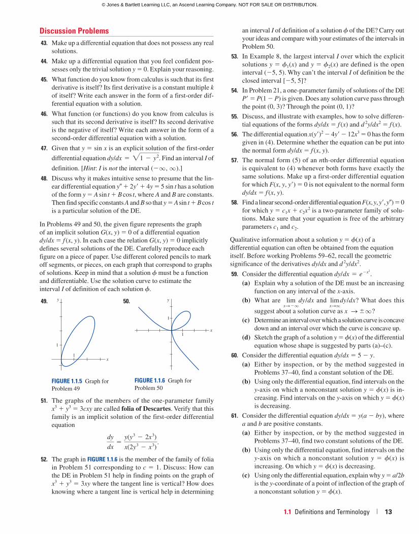
In Problems 49 and 50, the given figure represents the graph
of an implicit solution G(x, y) � 0 of a differential equation
dy/dx � f (x, y). In each case the relation G(x, y) � 0 implicitly
defines several solutions of the DE. Carefully reproduce each
figure on a piece of paper. Use different colored pencils to mark
off segments, or pieces, on each graph that correspond to graphs
of solutions. Keep in mind that a solution f must be a function
and differentiable. Use the solution curve to estimate the
interval I of definition of each solution f.
49.
FIGURE 1.1.5 Graph for
Problem 49
x
y
1
1
50.
FIGURE 1.1.6 Graph for
Problem 50
1
1x
y
51. The graphs of the members of the one-parameter family
x3 � y3 � 3cxy are called folia of Descartes. Verify that this
family is an implicit solution of the first-order differential
equation
dy
dx�
y(y3 2 2x3)
x(2y3 2 x3).
52. The graph in FIGURE 1.1.6 is the member of the family of folia
in Problem 51 corresponding to c � 1. Discuss: How can
the DE in Problem 51 help in finding points on the graph of
x3 � y3 � 3xy where the tangent line is vertical? How does
knowing where a tangent line is vertical help in determining
an interval I of definition of a solution f of the DE? Carry out
your ideas and compare with your estimates of the intervals in
Problem 50.
53. In Example 8, the largest interval I over which the explicit
solutions y � f1(x) and y � f2(x) are defined is the open
interval (�5, 5). Why can’t the interval I of definition be the
closed interval [�5, 5]?
54. In Problem 21, a one-parameter family of solutions of the DE
P� � P(1 � P) is given. Does any solution curve pass through
the point (0, 3)? Through the point (0, 1)?
55. Discuss, and illustrate with examples, how to solve differen-
tial equations of the forms dy/dx � f (x) and d 2y/dx2 � f (x).
56. The differential equation x(y�)2 � 4y� � 12x3 � 0 has the form
given in (4). Determine whether the equation can be put into
the normal form dy/dx � f (x, y).
57. The normal form (5) of an nth-order differential equation
is equivalent to (4) whenever both forms have exactly the
same solutions. Make up a first-order differential equation
for which F(x, y, y�) � 0 is not equivalent to the normal form
dy/dx � f (x, y).
58. Find a linear second-order differential equation F(x, y, y�, y�) � 0
for which y � c1x � c2x 2 is a two-parameter family of solu-
tions. Make sure that your equation is free of the arbitrary
parameters c1 and c2.
Qualitative information about a solution y � f(x) of a
differential equation can often be obtained from the equation
itself. Before working Problems 59–62, recall the geometric
significance of the derivatives dy/dx and d 2y/dx2.
59. Consider the differential equation dy/dx � e�x2
.
(a) Explain why a solution of the DE must be an increasing
function on any interval of the x-axis.
(b) What are limxS2q
dy/dx and limxSq
dy/dx? What does this
suggest about a solution curve as x Sq?
(c) Determine an interval over which a solution curve is concave
down and an interval over which the curve is concave up.
(d) Sketch the graph of a solution y � f(x) of the differential
equation whose shape is suggested by parts (a)–(c).
60. Consider the differential equation dy/dx � 5 � y.
(a) Either by inspection, or by the method suggested in
Problems 37–40, find a constant solution of the DE.
(b) Using only the differential equation, find intervals on the
y-axis on which a nonconstant solution y � f(x) is in-
creasing. Find intervals on the y-axis on which y � f(x)
is decreasing.
61. Consider the differential equation dy/dx � y(a � by), where
a and b are positive constants.
(a) Either by inspection, or by the method suggested in
Problems 37–40, find two constant solutions of the DE.
(b) Using only the differential equation, find intervals on the
y-axis on which a nonconstant solution y � f(x) is
increasing. On which y � f(x) is decreasing.
(c) Using only the differential equation, explain why y � a/2b
is the y-coordinate of a point of inflection of the graph of
a nonconstant solution y � f(x).
58229_CH01_001_031.indd Page 13 3/15/16 7:09 PM F-0017 58229_CH01_001_031.indd Page 13 3/15/16 7:09 PM F-0017 /202/JB00127/work/indd/202/JB00127/work/indd
© Jones & Bartlett Learning LLC, an Ascend Learning Company. NOT FOR SALE OR DISTRIBUTION.
© Jones & Bartlett Learning, LLCNOT FOR SALE OR DISTRIBUTION
© Jones & Bartlett Learning, LLCNOT FOR SALE OR DISTRIBUTION
© Jones & Bartlett Learning, LLCNOT FOR SALE OR DISTRIBUTION
© Jones & Bartlett Learning, LLCNOT FOR SALE OR DISTRIBUTION
© Jones & Bartlett Learning, LLCNOT FOR SALE OR DISTRIBUTION
© Jones & Bartlett Learning, LLCNOT FOR SALE OR DISTRIBUTION
© Jones & Bartlett Learning, LLCNOT FOR SALE OR DISTRIBUTION
© Jones & Bartlett Learning, LLCNOT FOR SALE OR DISTRIBUTION
© Jones & Bartlett Learning, LLCNOT FOR SALE OR DISTRIBUTION
© Jones & Bartlett Learning, LLCNOT FOR SALE OR DISTRIBUTION
© Jones & Bartlett Learning, LLCNOT FOR SALE OR DISTRIBUTION
© Jones & Bartlett Learning, LLCNOT FOR SALE OR DISTRIBUTION
© Jones & Bartlett Learning, LLCNOT FOR SALE OR DISTRIBUTION
© Jones & Bartlett Learning, LLCNOT FOR SALE OR DISTRIBUTION
© Jones & Bartlett Learning, LLCNOT FOR SALE OR DISTRIBUTION
© Jones & Bartlett Learning, LLCNOT FOR SALE OR DISTRIBUTION
© Jones & Bartlett Learning, LLCNOT FOR SALE OR DISTRIBUTION
© Jones & Bartlett Learning, LLCNOT FOR SALE OR DISTRIBUTION
© Jones & Bartlett Learning, LLCNOT FOR SALE OR DISTRIBUTION
© Jones & Bartlett Learning, LLCNOT FOR SALE OR DISTRIBUTION

14 | CHAPTER 1 Introduction to Differential Equations
(d) On the same coordinate axes, sketch the graphs of the two
constant solutions found in part (a). These constant solu-
tions partition the xy-plane into three regions. In each re-
gion, sketch the graph of a nonconstant solution y � f(x)
whose shape is suggested by the results in parts (b) and (c).
62. Consider the differential equation y� � y2 � 4.
(a) Explain why there exist no constant solutions of the DE.
(b) Describe the graph of a solution y � f(x). For example,
can a solution curve have any relative extrema?
(c) Explain why y � 0 is the y-coordinate of a point of inflec-
tion of a solution curve.
(d) Sketch the graph of a solution y � f(x) of the differential
equation whose shape is suggested by parts (a)–(c).
Computer Lab AssignmentsIn Problems 63 and 64, use a CAS to compute all derivatives
and to carry out the simplifications needed to verify that the
indicated function is a particular solution of the given differen-
tial equation.
63. y(4) � 20y� � 158y� � 580y� � 841y � 0;
y � xe5x cos 2x
64. x3y� � 2x2y� � 20xy� � 78y � 0;
y � 20 cos (5 ln x)
x2 3
sin (5 ln x)
x
1.2 Initial-Value Problems
INTRODUCTION We are often interested in problems in which we seek a solution y(x) of a
differential equation so that y(x) satisfies prescribed side conditions—that is, conditions that are
imposed on the unknown y(x) or on its derivatives. In this section we examine one such problem
called an initial-value problem.
Initial-Value Problem On some interval I containing x0, the problem
Solve: d n
y
dxn � f (x, y, y9, p , y(n21)) (1)
Subject to: y(x0) � y0, y9(x0) � y1, p , y(n21)(x0) � yn21,
where y0, y1, … , yn�1 are arbitrarily specified real constants, is called an initial-value problem (IVP). The values of y(x) and its first n�1 derivatives at a single point x0: y(x0) � y0, y�(x0) � y1, … ,
y(n�1)(x0) � yn�1, are called initial conditions (IC).
First- and Second-Order IVPs The problem given in (1) is also called an nth-order initial-value problem. For example,
Solve: dy
dx� f (x, y)
Subject to: y(x0) � y0
(2)
and Solve: d
2y
dx2� f (x, y, y9)
Subject to: y(x0) � y0, y9(x0) � y1
(3)
are first- and second-order initial-value problems, respectively. These two problems are easy
to interpret in geometric terms. For (2) we are seeking a solution of the differential equation on
an interval I containing x0 so that a solution curve passes through the prescribed point (x0, y0).
See FIGURE 1.2.1. For (3) we want to find a solution of the differential equation whose graph not
only passes through (x0, y0) but passes through so that the slope of the curve at this point is y1.
See FIGURE 1.2.2. The term initial condition derives from physical systems where the independent
variable is time t and where y(t0) � y0 and y�(t0) � y1 represent, respectively, the position and
velocity of an object at some beginning, or initial, time t0.
Solving an nth-order initial-value problem frequently entails using an n-parameter family of
solutions of the given differential equation to find n specialized constants so that the resulting
particular solution of the equation also “fits”—that is, satisfies—the n initial conditions.
y
x
solutions of the DE
I
(x0, y0)
FIGURE 1.2.1 First-order IVP
ysolutions of the DE
Ix
m = y1
(x0, y0)
FIGURE 1.2.2 Second-order IVP
58229_CH01_001_031.indd Page 14 6/18/16 5:50 AM F-0017 58229_CH01_001_031.indd Page 14 6/18/16 5:50 AM F-0017 /202/JB00127/work/indd/202/JB00127/work/indd
© Jones & Bartlett Learning LLC, an Ascend Learning Company. NOT FOR SALE OR DISTRIBUTION.
© Jones & Bartlett Learning, LLCNOT FOR SALE OR DISTRIBUTION
© Jones & Bartlett Learning, LLCNOT FOR SALE OR DISTRIBUTION
© Jones & Bartlett Learning, LLCNOT FOR SALE OR DISTRIBUTION
© Jones & Bartlett Learning, LLCNOT FOR SALE OR DISTRIBUTION
© Jones & Bartlett Learning, LLCNOT FOR SALE OR DISTRIBUTION
© Jones & Bartlett Learning, LLCNOT FOR SALE OR DISTRIBUTION
© Jones & Bartlett Learning, LLCNOT FOR SALE OR DISTRIBUTION
© Jones & Bartlett Learning, LLCNOT FOR SALE OR DISTRIBUTION
© Jones & Bartlett Learning, LLCNOT FOR SALE OR DISTRIBUTION
© Jones & Bartlett Learning, LLCNOT FOR SALE OR DISTRIBUTION
© Jones & Bartlett Learning, LLCNOT FOR SALE OR DISTRIBUTION
© Jones & Bartlett Learning, LLCNOT FOR SALE OR DISTRIBUTION
© Jones & Bartlett Learning, LLCNOT FOR SALE OR DISTRIBUTION
© Jones & Bartlett Learning, LLCNOT FOR SALE OR DISTRIBUTION
© Jones & Bartlett Learning, LLCNOT FOR SALE OR DISTRIBUTION
© Jones & Bartlett Learning, LLCNOT FOR SALE OR DISTRIBUTION
© Jones & Bartlett Learning, LLCNOT FOR SALE OR DISTRIBUTION
© Jones & Bartlett Learning, LLCNOT FOR SALE OR DISTRIBUTION
© Jones & Bartlett Learning, LLCNOT FOR SALE OR DISTRIBUTION
© Jones & Bartlett Learning, LLCNOT FOR SALE OR DISTRIBUTION
1.2 Initial-Value Problems | 15
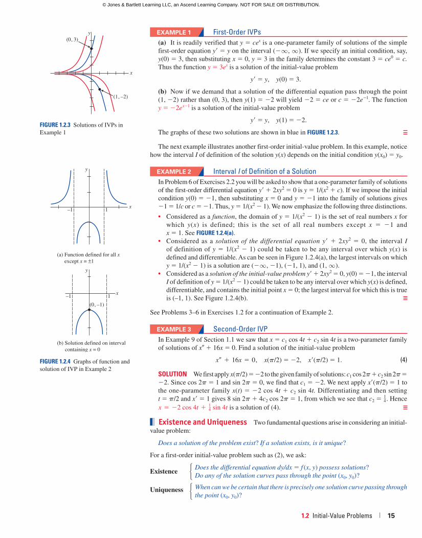
EXAMPLE 1 First-Order IVPs(a) It is readily verified that y � cex is a one-parameter family of solutions of the simple
first-order equation y� � y on the interval (�q , q ). If we specify an initial condition, say,
y(0) � 3, then substituting x � 0, y � 3 in the family determines the constant 3 � ce0 � c. Thus the function y � 3ex is a solution of the initial-value problem
y� � y, y(0) � 3.
(b) Now if we demand that a solution of the differential equation pass through the point
(1, �2) rather than (0, 3), then y(1) � �2 will yield �2 � ce or c � �2e�1. The function
y � �2e x�1 is a solution of the initial-value problem
y� � y, y(1) � �2.
The graphs of these two solutions are shown in blue in FIGURE 1.2.3.
The next example illustrates another first-order initial-value problem. In this example, notice
how the interval I of definition of the solution y(x) depends on the initial condition y(x0) � y0.
EXAMPLE 2 Interval I of Definition of a SolutionIn Problem 6 of Exercises 2.2 you will be asked to show that a one-parameter family of solutions
of the first-order differential equation y� � 2xy2 � 0 is y � 1/(x2 � c). If we impose the initial
condition y(0) � �1, then substituting x � 0 and y � �1 into the family of solutions gives
�1 � 1/c or c � �1. Thus, y � 1/(x2 � 1). We now emphasize the following three distinctions.
• Considered as a function, the domain of y � 1/(x2 � 1) is the set of real numbers x for
which y(x) is defined; this is the set of all real numbers except x � �1 and
x � 1. See FIGURE 1.2.4(a).• Considered as a solution of the differential equation y� � 2xy2 � 0, the interval I
of definition of y � 1/(x2 � 1) could be taken to be any interval over which y(x) is
defined and differentiable. As can be seen in Figure 1.2.4(a), the largest intervals on which
y � 1/(x2 � 1) is a solution are (�q , �1), (�1, 1), and (1, q ).
• Considered as a solution of the initial-value problem y� � 2xy2 � 0, y(0) � �1, the interval
I of definition of y � 1/(x2 � 1) could be taken to be any interval over which y(x) is defined,
differentiable, and contains the initial point x � 0; the largest interval for which this is true
is (–1, 1). See Figure 1.2.4(b).
See Problems 3–6 in Exercises 1.2 for a continuation of Example 2.
EXAMPLE 3 Second-Order IVPIn Example 9 of Section 1.1 we saw that x � c1 cos 4t � c2 sin 4t is a two-parameter family
of solutions of x� � 16x � 0. Find a solution of the initial-value problem
x0 � 16x � 0, x(p/2) � �2, x�(p/2) � 1. (4)
SOLUTION We first apply x(p/2) � �2 to the given family of solutions: c1 cos 2p � c2 sin 2p ��2. Since cos 2p � 1 and sin 2p � 0, we find that c1 � �2. We next apply x�(p/2) � 1 to
the one-parameter family x(t) � �2 cos 4t � c2 sin 4t. Differentiating and then setting
t � p/2 and x� � 1 gives 8 sin 2p � 4c2 cos 2p � 1, from which we see that c2 � 14. Hence
x � �2 cos 4t � 14 sin 4t is a solution of (4).
Existence and Uniqueness Two fundamental questions arise in considering an initial-
value problem:
Does a solution of the problem exist? If a solution exists, is it unique?
For a first-order initial-value problem such as (2), we ask:
Existence � Does the differential equation dy/dx � f (x, y) possess solutions?
Do any of the solution curves pass through the point (x0, y0)?
Uniqueness � When can we be certain that there is precisely one solution curve passing through the point (x0, y0)?
x
y
(1, –2)
(0, 3)
FIGURE 1.2.3 Solutions of IVPs in
Example 1
FIGURE 1.2.4 Graphs of function and
solution of IVP in Example 2
y
x–1 1
y
x–1 1
(a) Function defined for all x except x = ±1
(b) Solution defined on interval containing x = 0
(0, –1)
58229_CH01_001_031.indd Page 15 5/24/16 6:50 PM f-500 58229_CH01_001_031.indd Page 15 5/24/16 6:50 PM f-500 /202/JB00127/work/indd/202/JB00127/work/indd
© Jones & Bartlett Learning LLC, an Ascend Learning Company. NOT FOR SALE OR DISTRIBUTION.
© Jones & Bartlett Learning, LLCNOT FOR SALE OR DISTRIBUTION
© Jones & Bartlett Learning, LLCNOT FOR SALE OR DISTRIBUTION
© Jones & Bartlett Learning, LLCNOT FOR SALE OR DISTRIBUTION
© Jones & Bartlett Learning, LLCNOT FOR SALE OR DISTRIBUTION
© Jones & Bartlett Learning, LLCNOT FOR SALE OR DISTRIBUTION
© Jones & Bartlett Learning, LLCNOT FOR SALE OR DISTRIBUTION
© Jones & Bartlett Learning, LLCNOT FOR SALE OR DISTRIBUTION
© Jones & Bartlett Learning, LLCNOT FOR SALE OR DISTRIBUTION
© Jones & Bartlett Learning, LLCNOT FOR SALE OR DISTRIBUTION
© Jones & Bartlett Learning, LLCNOT FOR SALE OR DISTRIBUTION
© Jones & Bartlett Learning, LLCNOT FOR SALE OR DISTRIBUTION
© Jones & Bartlett Learning, LLCNOT FOR SALE OR DISTRIBUTION
© Jones & Bartlett Learning, LLCNOT FOR SALE OR DISTRIBUTION
© Jones & Bartlett Learning, LLCNOT FOR SALE OR DISTRIBUTION
© Jones & Bartlett Learning, LLCNOT FOR SALE OR DISTRIBUTION
© Jones & Bartlett Learning, LLCNOT FOR SALE OR DISTRIBUTION
© Jones & Bartlett Learning, LLCNOT FOR SALE OR DISTRIBUTION
© Jones & Bartlett Learning, LLCNOT FOR SALE OR DISTRIBUTION
© Jones & Bartlett Learning, LLCNOT FOR SALE OR DISTRIBUTION
© Jones & Bartlett Learning, LLCNOT FOR SALE OR DISTRIBUTION

16 | CHAPTER 1 Introduction to Differential Equations
Note that in Examples 1 and 3, the phrase “a solution” is used rather than “the solution” of the
problem. The indefinite article “a” is used deliberately to suggest the possibility that other solu-
tions may exist. At this point it has not been demonstrated that there is a single solution of each
problem. The next example illustrates an initial-value problem with two solutions.
EXAMPLE 4 An IVP Can Have Several SolutionsEach of the functions y � 0 and y � 1
16 x4 satisfies the differential equation dy/dx � xy1/2 and
the initial condition y(0) � 0, and so the initial-value problem dy/dx � xy1/2, y(0) � 0, has at
least two solutions. As illustrated in FIGURE 1.2.5, the graphs of both functions pass through
the same point (0, 0).
Within the safe confines of a formal course in differential equations one can be fairly con-
fident that most differential equations will have solutions and that solutions of initial-value
problems will probably be unique. Real life, however, is not so idyllic. Thus it is desirable to
know in advance of trying to solve an initial-value problem whether a solution exists and, when
it does, whether it is the only solution of the problem. Since we are going to consider first-
order differential equations in the next two chapters, we state here without proof a straight-
forward theorem that gives conditions that are sufficient to guarantee the existence and
uniqueness of a solution of a first-order initial-value problem of the form given in (2). We
shall wait until Chapter 3 to address the question of existence and uniqueness of a second-order
initial-value problem.
Theorem 1.2.1 Existence of a Unique Solution
Let R be a rectangular region in the xy-plane defined by a � x � b, c � y � d, that contains
the point (x0, y0) in its interior. If f (x, y) and f/ y are continuous on R, then there exists some
interval I0: (x0 � h, x0 � h), h � 0, contained in [a, b], and a unique function y(x) defined on
I0 that is a solution of the initial-value problem (2).
The foregoing result is one of the most popular existence and uniqueness theorems for first-
order differential equations, because the criteria of continuity of f (x, y) and f/ y are relatively
easy to check. The geometry of Theorem 1.2.1 is illustrated in FIGURE 1.2.6.
EXAMPLE 5 Example 4 RevisitedWe saw in Example 4 that the differential equation dy/dx � xy1/2 possesses at least two solu-
tions whose graphs pass through (0, 0). Inspection of the functions
f ( x, y) � xy1>2 and 0f
0y�
x
2y1>2shows that they are continuous in the upper half-plane defined by y � 0. Hence Theorem 1.2.1
enables us to conclude that through any point (x0, y0), y0 � 0, in the upper half-plane there
is some interval centered at x0 on which the given differential equation has a unique
solution. Thus, for example, even without solving it we know that there exists some
interval centered at 2 on which the initial-value problem dy/dx � xy1/2, y(2) � 1, has a
unique solution.
In Example 1, Theorem 1.2.1 guarantees that there are no other solutions of the initial-value
problems y� � y, y(0) � 3, and y� � y, y(1) � �2, other than y � 3e x and y � �2e x–1, respec-
tively. This follows from the fact that f (x, y) � y and f/ y � 1 are continuous throughout the
entire xy-plane. It can be further shown that the interval I on which each solution is defined
is (–q , q ).
Interval of Existence/Uniqueness Suppose y(x) represents a solution of the
initial-value problem (2). The following three sets on the real x-axis may not be the same:
the domain of the function y(x), the interval I over which the solution y(x) is defined or ex-
ists, and the interval I0 of existence and uniqueness. In Example 7 of Section 1.1 we illustrated
FIGURE 1.2.5 Two solutions of the same
IVP in Example 4
y
x(0, 0)
1
y = x4/16
y = 0
FIGURE 1.2.6 Rectangular region R
x
yd
c
a b
R
(x0, y0)
I0
58229_CH01_001_031.indd Page 16 3/15/16 7:09 PM F-0017 58229_CH01_001_031.indd Page 16 3/15/16 7:09 PM F-0017 /202/JB00127/work/indd/202/JB00127/work/indd
© Jones & Bartlett Learning LLC, an Ascend Learning Company. NOT FOR SALE OR DISTRIBUTION.
© Jones & Bartlett Learning, LLCNOT FOR SALE OR DISTRIBUTION
© Jones & Bartlett Learning, LLCNOT FOR SALE OR DISTRIBUTION
© Jones & Bartlett Learning, LLCNOT FOR SALE OR DISTRIBUTION
© Jones & Bartlett Learning, LLCNOT FOR SALE OR DISTRIBUTION
© Jones & Bartlett Learning, LLCNOT FOR SALE OR DISTRIBUTION
© Jones & Bartlett Learning, LLCNOT FOR SALE OR DISTRIBUTION
© Jones & Bartlett Learning, LLCNOT FOR SALE OR DISTRIBUTION
© Jones & Bartlett Learning, LLCNOT FOR SALE OR DISTRIBUTION
© Jones & Bartlett Learning, LLCNOT FOR SALE OR DISTRIBUTION
© Jones & Bartlett Learning, LLCNOT FOR SALE OR DISTRIBUTION
© Jones & Bartlett Learning, LLCNOT FOR SALE OR DISTRIBUTION
© Jones & Bartlett Learning, LLCNOT FOR SALE OR DISTRIBUTION
© Jones & Bartlett Learning, LLCNOT FOR SALE OR DISTRIBUTION
© Jones & Bartlett Learning, LLCNOT FOR SALE OR DISTRIBUTION
© Jones & Bartlett Learning, LLCNOT FOR SALE OR DISTRIBUTION
© Jones & Bartlett Learning, LLCNOT FOR SALE OR DISTRIBUTION
© Jones & Bartlett Learning, LLCNOT FOR SALE OR DISTRIBUTION
© Jones & Bartlett Learning, LLCNOT FOR SALE OR DISTRIBUTION
© Jones & Bartlett Learning, LLCNOT FOR SALE OR DISTRIBUTION
© Jones & Bartlett Learning, LLCNOT FOR SALE OR DISTRIBUTION
1.2 Initial-Value Problems | 17
the difference between the domain of a function and the interval I of definition. Now suppose
(x0, y0) is a point in the interior of the rectangular region R in Theorem 1.2.1. It turns out that the
continuity of the function f (x, y) on R by itself is sufficient to guarantee the existence of at least
one solution of dy/dx � f (x, y), y(x0) = y0, defined on some interval I. The interval I of definition
for this initial-value problem is usually taken to be the largest interval containing x0 over which
the solution y(x) is defined and differentiable. The interval I depends on both f (x, y) and the
initial condition y(x0) � y0. See Problems 31–34 in Exercises 1.2. The extra condition of continu-
ity of the first partial derivative �f/�y on R enables us to say that not only does a solution exist
on some interval I0 containing x0, but it also is the only solution satisfying y(x0) � y0. However,
Theorem 1.2.1 does not give any indication of the sizes of the intervals I and I0; the interval I of definition need not be as wide as the region R and the interval I0 of existence and uniqueness may not be as large as I. The number h � 0 that defines the interval I0: (x0 � h, x0 � h), could
be very small, and so it is best to think that the solution y(x) is unique in a local sense, that is, a
solution defined near the point (x0, y0). See Problem 50 in Exercises 1.2.
In Problems 1 and 2, y � 1/(1 � c1e–x) is a one-parameter family
of solutions of the first-order DE y� � y � y2. Find a solution of
the first-order IVP consisting of this differential equation and
the given initial condition.
1. y(0) � �13 2. y(�1) � 2
In Problems 3–6, y � 1/(x2 � c) is a one-parameter family of
solutions of the first-order DE y� � 2xy2 � 0. Find a solution
of the first-order IVP consisting of this differential equation and
the given initial condition. Give the largest interval I over which
the solution is defined.
3. y(2) � 13 4. y(�2) � 1
2
5. y(0) � 1 6. y (12) � �4
In Problems 7–10, x � c1 cos t � c2 sin t is a two-parameter
family of solutions of the second-order DE x � � x � 0. Find a
solution of the second-order IVP consisting of this differential
equation and the given initial conditions.
7. x(0) � �1, x�(0) � 8
8. x(p/2) � 0, x�(p/2) � 1
9. x(p/6) � 12, x�(p/6) � 0
10. x(p/4) � !2, x�(p/4) � 2!2
In Problems 11–14, y � c1ex � c2e
–x is a two-parameter family
of solutions of the second-order DE y � � y � 0. Find a solution
of the second-order IVP consisting of this differential equation
and the given initial conditions.
11. y(0) � 1, y�(0) � 2 12. y(1) � 0, y�(1) � e
13. y(�1) � 5, y�(�1) � �5 14. y(0) � 0, y�(0) � 0
In Problems 15 and 16, determine by inspection at least two
solutions of the given first-order IVP.
15. y� � 3y2/3, y(0) � 0 16. xy� � 2y, y(0) � 0
In Problems 17–24, determine a region of the xy-plane for which
the given differential equation would have a unique solution
whose graph passes through a point (x0, y0) in the region.
17. dy
dx� y2/3 18.
dy
dx� !xy
19. x dy
dx� y 20.
dy
dx2 y � x
Exercises Answers to selected odd-numbered problems begin on page ANS-1.1.2
REMARKS
(i) The conditions in Theorem 1.2.1 are sufficient but not necessary. When f (x, y) and �f/�y
are continuous on a rectangular region R, it must always follow that a solution of (2) exists
and is unique whenever (x0, y0) is a point interior to R. However, if the conditions stated
in the hypotheses of Theorem 1.2.1 do not hold, then anything could happen: Problem (2)
may still have a solution and this solution may be unique, or (2) may have several solutions,
or it may have no solution at all. A rereading of Example 4 reveals that the hypotheses of
Theorem 1.2.1 do not hold on the line y � 0 for the differential equation dy/dx � xy1/2, and
so it is not surprising, as we saw in Example 4 of this section, that there are two solutions
defined on a common interval (�h, h) satisfying y(0) � 0. On the other hand, the hypotheses
of Theorem 1.2.1 do not hold on the line y � 1 for the differential equation dy/dx � | y � 1|.
Nevertheless, it can be proved that the solution of the initial-value problem dy/dx � | y � 1|,
y(0) � 1, is unique. Can you guess this solution?
(ii) You are encouraged to read, think about, work, and then keep in mind Problem 49 in
Exercises 1.2.
58229_CH01_001_031.indd Page 17 6/28/16 11:17 PM F-0017 58229_CH01_001_031.indd Page 17 6/28/16 11:17 PM F-0017 /202/JB00127/work/indd/202/JB00127/work/indd
© Jones & Bartlett Learning LLC, an Ascend Learning Company. NOT FOR SALE OR DISTRIBUTION.
© Jones & Bartlett Learning, LLCNOT FOR SALE OR DISTRIBUTION
© Jones & Bartlett Learning, LLCNOT FOR SALE OR DISTRIBUTION
© Jones & Bartlett Learning, LLCNOT FOR SALE OR DISTRIBUTION
© Jones & Bartlett Learning, LLCNOT FOR SALE OR DISTRIBUTION
© Jones & Bartlett Learning, LLCNOT FOR SALE OR DISTRIBUTION
© Jones & Bartlett Learning, LLCNOT FOR SALE OR DISTRIBUTION
© Jones & Bartlett Learning, LLCNOT FOR SALE OR DISTRIBUTION
© Jones & Bartlett Learning, LLCNOT FOR SALE OR DISTRIBUTION
© Jones & Bartlett Learning, LLCNOT FOR SALE OR DISTRIBUTION
© Jones & Bartlett Learning, LLCNOT FOR SALE OR DISTRIBUTION
© Jones & Bartlett Learning, LLCNOT FOR SALE OR DISTRIBUTION
© Jones & Bartlett Learning, LLCNOT FOR SALE OR DISTRIBUTION
© Jones & Bartlett Learning, LLCNOT FOR SALE OR DISTRIBUTION
© Jones & Bartlett Learning, LLCNOT FOR SALE OR DISTRIBUTION
© Jones & Bartlett Learning, LLCNOT FOR SALE OR DISTRIBUTION
© Jones & Bartlett Learning, LLCNOT FOR SALE OR DISTRIBUTION
© Jones & Bartlett Learning, LLCNOT FOR SALE OR DISTRIBUTION
© Jones & Bartlett Learning, LLCNOT FOR SALE OR DISTRIBUTION
© Jones & Bartlett Learning, LLCNOT FOR SALE OR DISTRIBUTION
© Jones & Bartlett Learning, LLCNOT FOR SALE OR DISTRIBUTION

18 | CHAPTER 1 Introduction to Differential Equations
21. (4 2 y2)y9 � x2 22. (1 � y3)y9 � x2
23. (x2 � y2)y9 � y2 24. (y 2 x)y9 � y � x
In Problems 25–28, determine whether Theorem 1.2.1 guaran-
tees that the differential equation y9 � "y2 2 9 possesses a
unique solution through the given point.
25. (1, 4) 26. (5, 3)
27. (2, �3) 28. (�1, 1)
29. (a) By inspection, find a one-parameter family of solutions
of the differential equation xy� � y. Verify that each mem-
ber of the family is a solution of the initial-value problem
xy� � y, y(0) � 0.
(b) Explain part (a) by determining a region R in the xy-plane
for which the differential equation xy� � y would have a
unique solution through a point (x0, y0) in R.
(c) Verify that the piecewise-defined function
y � e0, x , 0
x, x $ 0
satisfies the condition y(0) � 0. Determine whether this
function is also a solution of the initial-value problem in
part (a).
30. (a) Verify that y � tan (x � c) is a one-parameter family of
solutions of the differential equation y� � 1 � y2.
(b) Since f (x, y) � 1 � y2 and f/ y � 2y are continuous
everywhere, the region R in Theorem 1.2.1 can be taken
to be the entire xy-plane. Use the family of solutions in
part (a) to find an explicit solution of the first-order initial-
value problem y� � 1 � y2, y(0) � 0. Even though x0 � 0
is in the interval (�2, 2), explain why the solution is not
defined on this interval.
(c) Determine the largest interval I of definition for the solu-
tion of the initial-value problem in part (b).
31. (a) Verify that y � –1/(x � c) is a one-parameter family of
solutions of the differential equation y� � y2.
(b) Since f (x, y) � y2 and f/ y � 2y are continuous every-
where, the region R in Theorem 1.2.1 can be taken to be
the entire xy-plane. Find a solution from the family in
part (a) that satisfies y(0) � 1. Find a solution from the
family in part (a) that satisfies y(0) � �1. Determine the
largest interval I of definition for the solution of each
initial-value problem.
32. (a) Find a solution from the family in part (a) of Problem 31
that satisfies y� � y2, y(0) � y0, where y0 � 0. Explain
why the largest interval I of definition for this solution is
either (�q , 1/y0) or (1/y0, q ).
(b) Determine the largest interval I of definition for the
solution of the first-order initial-value problem y� � y2,
y(0) � 0.
33. (a) Verify that 3x2 � y2 � c is a one-parameter family of
solutions of the differential equation y dy/dx � 3x.
(b) By hand, sketch the graph of the implicit solution
3x2 � y2 � 3. Find all explicit solutions y � f(x) of the
DE in part (a) defined by this relation. Give the interval I of definition of each explicit solution.
(c) The point (�2, 3) is on the graph of 3x2 � y2 � 3, but
which of the explicit solutions in part (b) satisfies
y(�2) � 3?
34. (a) Use the family of solutions in part (a) of Problem 33 to
find an implicit solution of the initial-value problem
y dy/dx � 3x, y(2) � �4. Then, by hand, sketch the graph
of the explicit solution of this problem and give its inter-
val I of definition.
(b) Are there any explicit solutions of y dy/dx � 3x that pass
through the origin?
In Problems 35–38, the graph of a member of a family of solu-
tions of a second-order differential equation d 2y/dx2 � f (x, y, y�) is given. Match the solution curve with at least one pair of the
following initial conditions.
(a) y(1) � 1, y�(1) � –2 (b) y(�1) � 0, y�(�1) � �4
(c) y(1) � 1, y�(1) � 2 (d) y(0) � �1, y�(0) � 2
(e) y(0) � �1, y�(0) � 0 (f ) y(0) � �4, y�(0) � –2
35.
x
y
5
5
–5
FIGURE 1.2.7 Graph for
Problem 35
36.
FIGURE 1.2.8 Graph for
Problem 36
x
y
5
5
–5
37.
FIGURE 1.2.9 Graph for
Problem 37
x
y
5
5
–5
38.
FIGURE 1.2.10 Graph for
Problem 38
x
y
5
5
–5
In Problems 39–44, y � c1 cos 3x � c2 sin 3x is a two-parameter
family of solutions of the second-order DE y� � 9y � 0. If pos-
sible, find a solution of the differential equation that satisfies the
given side conditions. The conditions specified at two different
points are called boundary conditions.
39. y(0) � 0, y(p/6) � �1 40. y(0) � 0, y(p) � 0
41. y�(0) � 0, y�(p/4) � 0 42. y(0) � 1, y�(p) � 5
43. y(0) � 0, y(p) � 4 44. y�(p/3) � 1, y�(p) � 0
Discussion ProblemsIn Problems 45 and 46, use Problem 55 in Exercises 1.1 and (2)
and (3) of this section.
45. Find a function y � f (x) whose graph at each point (x, y) has
the slope given by 8e2x � 6x and has the y-intercept (0, 9).
58229_CH01_001_031.indd Page 18 3/15/16 7:09 PM F-0017 58229_CH01_001_031.indd Page 18 3/15/16 7:09 PM F-0017 /202/JB00127/work/indd/202/JB00127/work/indd
© Jones & Bartlett Learning LLC, an Ascend Learning Company. NOT FOR SALE OR DISTRIBUTION.
© Jones & Bartlett Learning, LLCNOT FOR SALE OR DISTRIBUTION
© Jones & Bartlett Learning, LLCNOT FOR SALE OR DISTRIBUTION
© Jones & Bartlett Learning, LLCNOT FOR SALE OR DISTRIBUTION
© Jones & Bartlett Learning, LLCNOT FOR SALE OR DISTRIBUTION
© Jones & Bartlett Learning, LLCNOT FOR SALE OR DISTRIBUTION
© Jones & Bartlett Learning, LLCNOT FOR SALE OR DISTRIBUTION
© Jones & Bartlett Learning, LLCNOT FOR SALE OR DISTRIBUTION
© Jones & Bartlett Learning, LLCNOT FOR SALE OR DISTRIBUTION
© Jones & Bartlett Learning, LLCNOT FOR SALE OR DISTRIBUTION
© Jones & Bartlett Learning, LLCNOT FOR SALE OR DISTRIBUTION
© Jones & Bartlett Learning, LLCNOT FOR SALE OR DISTRIBUTION
© Jones & Bartlett Learning, LLCNOT FOR SALE OR DISTRIBUTION
© Jones & Bartlett Learning, LLCNOT FOR SALE OR DISTRIBUTION
© Jones & Bartlett Learning, LLCNOT FOR SALE OR DISTRIBUTION
© Jones & Bartlett Learning, LLCNOT FOR SALE OR DISTRIBUTION
© Jones & Bartlett Learning, LLCNOT FOR SALE OR DISTRIBUTION
© Jones & Bartlett Learning, LLCNOT FOR SALE OR DISTRIBUTION
© Jones & Bartlett Learning, LLCNOT FOR SALE OR DISTRIBUTION
© Jones & Bartlett Learning, LLCNOT FOR SALE OR DISTRIBUTION
© Jones & Bartlett Learning, LLCNOT FOR SALE OR DISTRIBUTION
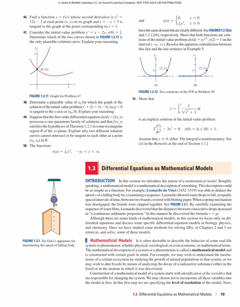
1.3 Differential Equations as Mathematical Models | 19
46. Find a function y � f (x) whose second derivative is y� �
12x � 2 at each point (x, y) on its graph and y � �x � 5 is
tangent to the graph at the point corresponding to x � 1.
47. Consider the initial-value problem y� � x � 2y, y(0) � 12 .
Determine which of the two curves shown in FIGURE 1.2.11 is
the only plausible solution curve. Explain your reasoning.
x
y1
1
(0, ¹⁄₂)
FIGURE 1.2.11 Graph for Problem 47
48. Determine a plausible value of x0 for which the graph of the
solution of the initial-value problem y� � 2y � 3x � 6, y(x0) � 0
is tangent to the x-axis at (x0, 0). Explain your reasoning.
49. Suppose that the first-order differential equation dy/dx � f (x, y)
possesses a one-parameter family of solutions and that f (x, y)
satisfies the hypotheses of Theorem 1.2.1 in some rectangular
region R of the xy-plane. Explain why two different solution
curves cannot intersect or be tangent to each other at a point
(x0, y0) in R.
50. The functions
y(x) � 116 x4, �q , x , q
and y(x) � e 0, x , 01
16 x4, x $ 0
have the same domain but are clearly different. See FIGURES 1.2.12(a) and 1.2.12(b), respectively. Show that both functions are solu-
tions of the initial-value problem dy/dx � xy1/2, y(2) � 1 on the
interval (–q , q). Resolve the apparent contradiction between
this fact and the last sentence in Example 5.
FIGURE 1.2.12 Two solutions of the IVP in Problem 50
y
x
(2, 1)1
(a)
y
x
(2, 1)1
(b)
51. Show that
x � #y
0
1"t3 � 1 dt
is an implicit solution of the initial-value problem
2
d 2y
dx22 3y2 � 0, y(0) � 0, y9(0) � 1.
Assume that y $ 0. [Hint: The integral is nonelementary. See
(ii) in the Remarks at the end of Section 1.1.]
1.3 Differential Equations as Mathematical Models
INTRODUCTION In this section we introduce the notion of a mathematical model. Roughly
speaking, a mathematical model is a mathematical description of something. This description could
be as simple as a function. For example, Leonardo da Vinci (1452–1519) was able to deduce the
speed v of a falling body by a examining a sequence. Leonardo allowed water drops to fall, at equally
spaced intervals of time, between two boards covered with blotting paper. When a spring mechanism
was disengaged, the boards were clapped together. See FIGURE 1.3.1. By carefully examining the
sequence of water blots, Leonardo discovered that the distances between consecutive drops increased
in “a continuous arithmetic proportion.” In this manner he discovered the formula v � gt.Although there are many kinds of mathematical models, in this section we focus only on dif-
ferential equations and discuss some specific differential-equation models in biology, physics,
and chemistry. Once we have studied some methods for solving DEs, in Chapters 2 and 3 we
return to, and solve, some of these models.
Mathematical Models It is often desirable to describe the behavior of some real-life
system or phenomenon, whether physical, sociological, or even economic, in mathematical terms.
The mathematical description of a system or a phenomenon is called a mathematical model and
is constructed with certain goals in mind. For example, we may wish to understand the mecha-
nisms of a certain ecosystem by studying the growth of animal populations in that system, or we
may wish to date fossils by means of analyzing the decay of a radioactive substance either in the
fossil or in the stratum in which it was discovered.
Construction of a mathematical model of a system starts with identification of the variables that
are responsible for changing the system. We may choose not to incorporate all these variables into
the model at first. In this first step we are specifying the level of resolution of the model. Next,
FIGURE 1.3.1 Da Vinci’s apparatus for
determining the speed of falling body
58229_CH01_001_031.indd Page 19 5/24/16 6:50 PM f-500 58229_CH01_001_031.indd Page 19 5/24/16 6:50 PM f-500 /202/JB00127/work/indd/202/JB00127/work/indd
© Jones & Bartlett Learning LLC, an Ascend Learning Company. NOT FOR SALE OR DISTRIBUTION.
© Jones & Bartlett Learning, LLCNOT FOR SALE OR DISTRIBUTION
© Jones & Bartlett Learning, LLCNOT FOR SALE OR DISTRIBUTION
© Jones & Bartlett Learning, LLCNOT FOR SALE OR DISTRIBUTION
© Jones & Bartlett Learning, LLCNOT FOR SALE OR DISTRIBUTION
© Jones & Bartlett Learning, LLCNOT FOR SALE OR DISTRIBUTION
© Jones & Bartlett Learning, LLCNOT FOR SALE OR DISTRIBUTION
© Jones & Bartlett Learning, LLCNOT FOR SALE OR DISTRIBUTION
© Jones & Bartlett Learning, LLCNOT FOR SALE OR DISTRIBUTION
© Jones & Bartlett Learning, LLCNOT FOR SALE OR DISTRIBUTION
© Jones & Bartlett Learning, LLCNOT FOR SALE OR DISTRIBUTION
© Jones & Bartlett Learning, LLCNOT FOR SALE OR DISTRIBUTION
© Jones & Bartlett Learning, LLCNOT FOR SALE OR DISTRIBUTION
© Jones & Bartlett Learning, LLCNOT FOR SALE OR DISTRIBUTION
© Jones & Bartlett Learning, LLCNOT FOR SALE OR DISTRIBUTION
© Jones & Bartlett Learning, LLCNOT FOR SALE OR DISTRIBUTION
© Jones & Bartlett Learning, LLCNOT FOR SALE OR DISTRIBUTION
© Jones & Bartlett Learning, LLCNOT FOR SALE OR DISTRIBUTION
© Jones & Bartlett Learning, LLCNOT FOR SALE OR DISTRIBUTION
© Jones & Bartlett Learning, LLCNOT FOR SALE OR DISTRIBUTION
© Jones & Bartlett Learning, LLCNOT FOR SALE OR DISTRIBUTION
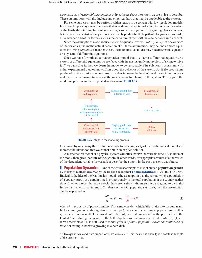
20 | CHAPTER 1 Introduction to Differential Equations
we make a set of reasonable assumptions or hypotheses about the system we are trying to describe.
These assumptions will also include any empirical laws that may be applicable to the system.
For some purposes it may be perfectly within reason to be content with low-resolution models.
For example, you may already be aware that in modeling the motion of a body falling near the surface
of the Earth, the retarding force of air friction, is sometimes ignored in beginning physics courses;
but if you are a scientist whose job it is to accurately predict the flight path of a long-range projectile,
air resistance and other factors such as the curvature of the Earth have to be taken into account.
Since the assumptions made about a system frequently involve a rate of change of one or more
of the variables, the mathematical depiction of all these assumptions may be one or more equa-
tions involving derivatives. In other words, the mathematical model may be a differential equation
or a system of differential equations.
Once we have formulated a mathematical model that is either a differential equation or a
system of differential equations, we are faced with the not insignificant problem of trying to solve
it. If we can solve it, then we deem the model to be reasonable if its solution is consistent with
either experimental data or known facts about the behavior of the system. But if the predictions
produced by the solution are poor, we can either increase the level of resolution of the model or
make alternative assumptions about the mechanisms for change in the system. The steps of the
modeling process are then repeated as shown in FIGURE 1.3.2.
Assumptionsand hypotheses
Mathematicalformulation
Check modelpredictions with
known facts
Obtainsolutions
Express assumptionsin terms of DEs
Display predictionsof the model
(e.g., graphically)
If necessary,alter assumptions
or increase resolutionof the model
Solve the DEs
FIGURE 1.3.2 Steps in the modeling process
Of course, by increasing the resolution we add to the complexity of the mathematical model and
increase the likelihood that we cannot obtain an explicit solution.
A mathematical model of a physical system will often involve the variable time t. A solution of
the model then gives the state of the system; in other words, for appropriate values of t, the values
of the dependent variable (or variables) describe the system in the past, present, and future.
Population Dynamics One of the earliest attempts to model human population growth
by means of mathematics was by the English economist Thomas Malthus (1776–1834) in 1798.
Basically, the idea of the Malthusian model is the assumption that the rate at which a population
of a country grows at a certain time is proportional* to the total population of the country at that
time. In other words, the more people there are at time t, the more there are going to be in the
future. In mathematical terms, if P(t) denotes the total population at time t, then this assumption
can be expressed as
dP
dtr P or
dP
dt� kP, (1)
where k is a constant of proportionality. This simple model, which fails to take into account many
factors (immigration and emigration, for example) that can influence human populations to either
grow or decline, nevertheless turned out to be fairly accurate in predicting the population of the
United States during the years 1790–1860. Populations that grow at a rate described by (1) are
rare; nevertheless, (1) is still used to model growth of small populations over short intervals of time, for example, bacteria growing in a petri dish.
*If two quantities u and v are proportional, we write u ~ v. This means one quantity is a constant multiple
of the other: u � kv.
58229_CH01_001_031.indd Page 20 3/15/16 7:09 PM F-0017 58229_CH01_001_031.indd Page 20 3/15/16 7:09 PM F-0017 /202/JB00127/work/indd/202/JB00127/work/indd
© Jones & Bartlett Learning LLC, an Ascend Learning Company. NOT FOR SALE OR DISTRIBUTION.
© Jones & Bartlett Learning, LLCNOT FOR SALE OR DISTRIBUTION
© Jones & Bartlett Learning, LLCNOT FOR SALE OR DISTRIBUTION
© Jones & Bartlett Learning, LLCNOT FOR SALE OR DISTRIBUTION
© Jones & Bartlett Learning, LLCNOT FOR SALE OR DISTRIBUTION
© Jones & Bartlett Learning, LLCNOT FOR SALE OR DISTRIBUTION
© Jones & Bartlett Learning, LLCNOT FOR SALE OR DISTRIBUTION
© Jones & Bartlett Learning, LLCNOT FOR SALE OR DISTRIBUTION
© Jones & Bartlett Learning, LLCNOT FOR SALE OR DISTRIBUTION
© Jones & Bartlett Learning, LLCNOT FOR SALE OR DISTRIBUTION
© Jones & Bartlett Learning, LLCNOT FOR SALE OR DISTRIBUTION
© Jones & Bartlett Learning, LLCNOT FOR SALE OR DISTRIBUTION
© Jones & Bartlett Learning, LLCNOT FOR SALE OR DISTRIBUTION
© Jones & Bartlett Learning, LLCNOT FOR SALE OR DISTRIBUTION
© Jones & Bartlett Learning, LLCNOT FOR SALE OR DISTRIBUTION
© Jones & Bartlett Learning, LLCNOT FOR SALE OR DISTRIBUTION
© Jones & Bartlett Learning, LLCNOT FOR SALE OR DISTRIBUTION
© Jones & Bartlett Learning, LLCNOT FOR SALE OR DISTRIBUTION
© Jones & Bartlett Learning, LLCNOT FOR SALE OR DISTRIBUTION
© Jones & Bartlett Learning, LLCNOT FOR SALE OR DISTRIBUTION
© Jones & Bartlett Learning, LLCNOT FOR SALE OR DISTRIBUTION
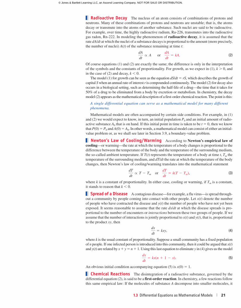
1.3 Differential Equations as Mathematical Models | 21
Radioactive Decay The nucleus of an atom consists of combinations of protons and
neutrons. Many of these combinations of protons and neutrons are unstable; that is, the atoms
decay or transmute into the atoms of another substance. Such nuclei are said to be radioactive.
For example, over time, the highly radioactive radium, Ra-226, transmutes into the radioactive
gas radon, Rn-222. In modeling the phenomenon of radioactive decay, it is assumed that the
rate dA/dt at which the nuclei of a substance decays is proportional to the amount (more precisely,
the number of nuclei) A(t) of the substance remaining at time t:
dA
dtr A or
dA
dt� kA. (2)
Of course equations (1) and (2) are exactly the same; the difference is only in the interpretation
of the symbols and the constants of proportionality. For growth, as we expect in (1), k � 0, and
in the case of (2) and decay, k 0.
The model (1) for growth can be seen as the equation dS/dt � rS, which describes the growth of
capital S when an annual rate of interest r is compounded continuously. The model (2) for decay also
occurs in a biological setting, such as determining the half-life of a drug—the time that it takes for
50% of a drug to be eliminated from a body by excretion or metabolism. In chemistry, the decay
model (2) appears as the mathematical description of a first-order chemical reaction. The point is this:
A single differential equation can serve as a mathematical model for many different phenomena.
Mathematical models are often accompanied by certain side conditions. For example, in (1)
and (2) we would expect to know, in turn, an initial population P0 and an initial amount of radio-
active substance A0 that is on hand. If this initial point in time is taken to be t � 0, then we know
that P(0) � P0 and A(0) � A0. In other words, a mathematical model can consist of either an initial-
value problem or, as we shall see later in Section 3.9, a boundary-value problem.
Newton’s Law of Cooling/Warming According to Newton’s empirical law of cooling—or warming—the rate at which the temperature of a body changes is proportional to the
difference between the temperature of the body and the temperature of the surrounding medium,
the so-called ambient temperature. If T(t) represents the temperature of a body at time t, Tm the
temperature of the surrounding medium, and dT/dt the rate at which the temperature of the body
changes, then Newton’s law of cooling/warming translates into the mathematical statement
dT
dtr T 2 Tm or
dT
dt� k(T 2 Tm), (3)
where k is a constant of proportionality. In either case, cooling or warming, if Tm is a constant,
it stands to reason that k 0.
Spread of a Disease A contagious disease—for example, a flu virus—is spread through-
out a community by people coming into contact with other people. Let x(t) denote the number
of people who have contracted the disease and y(t) the number of people who have not yet been
exposed. It seems reasonable to assume that the rate dx/dt at which the disease spreads is pro-
portional to the number of encounters or interactions between these two groups of people. If we
assume that the number of interactions is jointly proportional to x(t) and y(t), that is, proportional
to the product xy, then
dx
dt� kxy, (4)
where k is the usual constant of proportionality. Suppose a small community has a fixed population
of n people. If one infected person is introduced into this community, then it could be argued that x(t) and y(t) are related by x � y � n � 1. Using this last equation to eliminate y in (4) gives us the model
dx
dt� kx(n � 1 2 x). (5)
An obvious initial condition accompanying equation (5) is x(0) � 1.
Chemical Reactions The disintegration of a radioactive substance, governed by the
differential equation (2), is said to be a first-order reaction. In chemistry, a few reactions follow
this same empirical law: If the molecules of substance A decompose into smaller molecules, it
58229_CH01_001_031.indd Page 21 3/15/16 7:09 PM F-0017 58229_CH01_001_031.indd Page 21 3/15/16 7:09 PM F-0017 /202/JB00127/work/indd/202/JB00127/work/indd
© Jones & Bartlett Learning LLC, an Ascend Learning Company. NOT FOR SALE OR DISTRIBUTION.
© Jones & Bartlett Learning, LLCNOT FOR SALE OR DISTRIBUTION
© Jones & Bartlett Learning, LLCNOT FOR SALE OR DISTRIBUTION
© Jones & Bartlett Learning, LLCNOT FOR SALE OR DISTRIBUTION
© Jones & Bartlett Learning, LLCNOT FOR SALE OR DISTRIBUTION
© Jones & Bartlett Learning, LLCNOT FOR SALE OR DISTRIBUTION
© Jones & Bartlett Learning, LLCNOT FOR SALE OR DISTRIBUTION
© Jones & Bartlett Learning, LLCNOT FOR SALE OR DISTRIBUTION
© Jones & Bartlett Learning, LLCNOT FOR SALE OR DISTRIBUTION
© Jones & Bartlett Learning, LLCNOT FOR SALE OR DISTRIBUTION
© Jones & Bartlett Learning, LLCNOT FOR SALE OR DISTRIBUTION
© Jones & Bartlett Learning, LLCNOT FOR SALE OR DISTRIBUTION
© Jones & Bartlett Learning, LLCNOT FOR SALE OR DISTRIBUTION
© Jones & Bartlett Learning, LLCNOT FOR SALE OR DISTRIBUTION
© Jones & Bartlett Learning, LLCNOT FOR SALE OR DISTRIBUTION
© Jones & Bartlett Learning, LLCNOT FOR SALE OR DISTRIBUTION
© Jones & Bartlett Learning, LLCNOT FOR SALE OR DISTRIBUTION
© Jones & Bartlett Learning, LLCNOT FOR SALE OR DISTRIBUTION
© Jones & Bartlett Learning, LLCNOT FOR SALE OR DISTRIBUTION
© Jones & Bartlett Learning, LLCNOT FOR SALE OR DISTRIBUTION
© Jones & Bartlett Learning, LLCNOT FOR SALE OR DISTRIBUTION
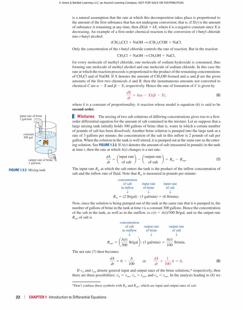
22 | CHAPTER 1 Introduction to Differential Equations
is a natural assumption that the rate at which this decomposition takes place is proportional to
the amount of the first substance that has not undergone conversion; that is, if X(t) is the amount
of substance A remaining at any time, then dX/dt � kX, where k is a negative constant since X is
decreasing. An example of a first-order chemical reaction is the conversion of t-butyl chloride
into t-butyl alcohol:
(CH3)3CCl � NaOH S (CH3)3COH � NaCl.
Only the concentration of the t-butyl chloride controls the rate of reaction. But in the reaction
CH3Cl � NaOH S CH3OH � NaCl,
for every molecule of methyl chloride, one molecule of sodium hydroxide is consumed, thus
forming one molecule of methyl alcohol and one molecule of sodium chloride. In this case the
rate at which the reaction proceeds is proportional to the product of the remaining concentrations
of CH3Cl and of NaOH. If X denotes the amount of CH3OH formed and a and b are the given
amounts of the first two chemicals A and B, then the instantaneous amounts not converted to
chemical C are a � X and b � X, respectively. Hence the rate of formation of C is given by
dX
dt� k(a 2 X)(b 2 X), (6)
where k is a constant of proportionality. A reaction whose model is equation (6) is said to be
second order.
Mixtures The mixing of two salt solutions of differing concentrations gives rise to a first-
order differential equation for the amount of salt contained in the mixture. Let us suppose that a
large mixing tank initially holds 300 gallons of brine (that is, water in which a certain number
of pounds of salt has been dissolved). Another brine solution is pumped into the large tank at a
rate of 3 gallons per minute; the concentration of the salt in this inflow is 2 pounds of salt per
gallon. When the solution in the tank is well stirred, it is pumped out at the same rate as the enter-
ing solution. See FIGURE 1.3.3. If A(t) denotes the amount of salt (measured in pounds) in the tank
at time t, then the rate at which A(t) changes is a net rate:
dA
dt� ainput rate
of saltb 2 aoutput rate
of saltb � Rin 2 Rout. (7)
The input rate Rin at which the salt enters the tank is the product of the inflow concentration of
salt and the inflow rate of fluid. Note that Rin is measured in pounds per minute:
concentration of salt input rate input rate in inflow of brine of salt
T T T
Rin � (2 lb/gal) � (3 gal/min) � (6 lb/min).
Now, since the solution is being pumped out of the tank at the same rate that it is pumped in, the
number of gallons of brine in the tank at time t is a constant 300 gallons. Hence the concentration
of the salt in the tank, as well as in the outflow, is c(t) � A(t)/300 lb/gal, and so the output rate
Rout of salt is
concentration of salt output rate output rate in outflow of brine of salt
T T T
Rout � aA(t)
300 lb/galb � (3 gal/min) �
A(t)
100 lb/min.
The net rate (7) then becomes
dA
dt� 6 2
A
100 or
dA
dt�
1
100 A � 6. (8)
If rin and rout denote general input and output rates of the brine solutions,* respectively, then
there are three possibilities: rin � rout , rin � rout , and rin rout . In the analysis leading to (8) we
FIGURE 1.3.3 Mixing tank
constant300 gal
input rate of brine3 gal/min
output rate of brine3 gal/min
*Don’t confuse these symbols with Rin and Rout , which are input and output rates of salt.
58229_CH01_001_031.indd Page 22 3/15/16 7:09 PM F-0017 58229_CH01_001_031.indd Page 22 3/15/16 7:09 PM F-0017 /202/JB00127/work/indd/202/JB00127/work/indd
© Jones & Bartlett Learning LLC, an Ascend Learning Company. NOT FOR SALE OR DISTRIBUTION.
© Jones & Bartlett Learning, LLCNOT FOR SALE OR DISTRIBUTION
© Jones & Bartlett Learning, LLCNOT FOR SALE OR DISTRIBUTION
© Jones & Bartlett Learning, LLCNOT FOR SALE OR DISTRIBUTION
© Jones & Bartlett Learning, LLCNOT FOR SALE OR DISTRIBUTION
© Jones & Bartlett Learning, LLCNOT FOR SALE OR DISTRIBUTION
© Jones & Bartlett Learning, LLCNOT FOR SALE OR DISTRIBUTION
© Jones & Bartlett Learning, LLCNOT FOR SALE OR DISTRIBUTION
© Jones & Bartlett Learning, LLCNOT FOR SALE OR DISTRIBUTION
© Jones & Bartlett Learning, LLCNOT FOR SALE OR DISTRIBUTION
© Jones & Bartlett Learning, LLCNOT FOR SALE OR DISTRIBUTION
© Jones & Bartlett Learning, LLCNOT FOR SALE OR DISTRIBUTION
© Jones & Bartlett Learning, LLCNOT FOR SALE OR DISTRIBUTION
© Jones & Bartlett Learning, LLCNOT FOR SALE OR DISTRIBUTION
© Jones & Bartlett Learning, LLCNOT FOR SALE OR DISTRIBUTION
© Jones & Bartlett Learning, LLCNOT FOR SALE OR DISTRIBUTION
© Jones & Bartlett Learning, LLCNOT FOR SALE OR DISTRIBUTION
© Jones & Bartlett Learning, LLCNOT FOR SALE OR DISTRIBUTION
© Jones & Bartlett Learning, LLCNOT FOR SALE OR DISTRIBUTION
© Jones & Bartlett Learning, LLCNOT FOR SALE OR DISTRIBUTION
© Jones & Bartlett Learning, LLCNOT FOR SALE OR DISTRIBUTION
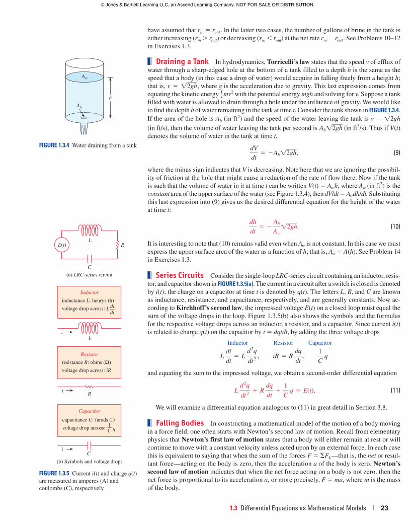
1.3 Differential Equations as Mathematical Models | 23
have assumed that rin � rout . In the latter two cases, the number of gallons of brine in the tank is
either increasing (rin � rout) or decreasing (rin rout) at the net rate rin � rout . See Problems 10–12
in Exercises 1.3.
Draining a Tank In hydrodynamics, Torricelli’s law states that the speed v of efflux of
water through a sharp-edged hole at the bottom of a tank filled to a depth h is the same as the
speed that a body (in this case a drop of water) would acquire in falling freely from a height h;
that is, v � !2gh, where g is the acceleration due to gravity. This last expression comes from
equating the kinetic energy 12 mv2 with the potential energy mgh and solving for v. Suppose a tank
filled with water is allowed to drain through a hole under the influence of gravity. We would like
to find the depth h of water remaining in the tank at time t. Consider the tank shown in FIGURE 1.3.4.
If the area of the hole is Ah (in ft2) and the speed of the water leaving the tank is v � !2gh
(in ft/s), then the volume of water leaving the tank per second is Ah!2gh (in ft3/s). Thus if V(t) denotes the volume of water in the tank at time t,
dV
dt� �Ah!2gh, (9)
where the minus sign indicates that V is decreasing. Note here that we are ignoring the possibil-
ity of friction at the hole that might cause a reduction of the rate of flow there. Now if the tank
is such that the volume of water in it at time t can be written V(t) � Aw h, where Aw (in ft2) is the
constant area of the upper surface of the water (see Figure 1.3.4), then dV/dt � Awdh/dt. Substituting
this last expression into (9) gives us the desired differential equation for the height of the water
at time t:
dh
dt� �
Ah
Aw
!2gh. (10)
It is interesting to note that (10) remains valid even when Aw is not constant. In this case we must
express the upper surface area of the water as a function of h; that is, Aw � A(h). See Problem 14
in Exercises 1.3.
Series Circuits Consider the single-loop LRC-series circuit containing an inductor, resis-
tor, and capacitor shown in FIGURE 1.3.5(a). The current in a circuit after a switch is closed is denoted
by i(t); the charge on a capacitor at time t is denoted by q(t). The letters L, R, and C are known
as inductance, resistance, and capacitance, respectively, and are generally constants. Now ac-
cording to Kirchhoff’s second law, the impressed voltage E(t) on a closed loop must equal the
sum of the voltage drops in the loop. Figure 1.3.5(b) also shows the symbols and the formulas
for the respective voltage drops across an inductor, a resistor, and a capacitor. Since current i(t) is related to charge q(t) on the capacitor by i � dq/dt, by adding the three voltage drops
Inductor Resistor Capacitor
L di
dt� L
d 2q
dt 2
, iR � R dq
dt,
1
C q
and equating the sum to the impressed voltage, we obtain a second-order differential equation
L d
2q
dt 2
� R dq
dt�
1
C q � E(t). (11)
We will examine a differential equation analogous to (11) in great detail in Section 3.8.
Falling Bodies In constructing a mathematical model of the motion of a body moving
in a force field, one often starts with Newton’s second law of motion. Recall from elementary
physics that Newton’s first law of motion states that a body will either remain at rest or will
continue to move with a constant velocity unless acted upon by an external force. In each case
this is equivalent to saying that when the sum of the forces F � �Fk —that is, the net or resul-
tant force—acting on the body is zero, then the acceleration a of the body is zero. Newton’s second law of motion indicates that when the net force acting on a body is not zero, then the
net force is proportional to its acceleration a, or more precisely, F � ma, where m is the mass
of the body.
FIGURE 1.3.4 Water draining from a tank
Aw
Ah
h
FIGURE 1.3.5 Current i(t) and charge q(t) are measured in amperes (A) and
coulombs (C), respectively
Inductor
didt
Li
Resistor
C
i R
i
Capacitor
q1C
(a) LRC-series circuit
(b) Symbols and voltage drops
LR
C
E(t)
resistance R: ohms (Ω)
voltage drop across: iR
capacitance C: farads (f)
voltage drop across:
inductance L: henrys (h)
voltage drop across: L
58229_CH01_001_031.indd Page 23 3/15/16 7:09 PM F-0017 58229_CH01_001_031.indd Page 23 3/15/16 7:09 PM F-0017 /202/JB00127/work/indd/202/JB00127/work/indd
© Jones & Bartlett Learning LLC, an Ascend Learning Company. NOT FOR SALE OR DISTRIBUTION.
© Jones & Bartlett Learning, LLCNOT FOR SALE OR DISTRIBUTION
© Jones & Bartlett Learning, LLCNOT FOR SALE OR DISTRIBUTION
© Jones & Bartlett Learning, LLCNOT FOR SALE OR DISTRIBUTION
© Jones & Bartlett Learning, LLCNOT FOR SALE OR DISTRIBUTION
© Jones & Bartlett Learning, LLCNOT FOR SALE OR DISTRIBUTION
© Jones & Bartlett Learning, LLCNOT FOR SALE OR DISTRIBUTION
© Jones & Bartlett Learning, LLCNOT FOR SALE OR DISTRIBUTION
© Jones & Bartlett Learning, LLCNOT FOR SALE OR DISTRIBUTION
© Jones & Bartlett Learning, LLCNOT FOR SALE OR DISTRIBUTION
© Jones & Bartlett Learning, LLCNOT FOR SALE OR DISTRIBUTION
© Jones & Bartlett Learning, LLCNOT FOR SALE OR DISTRIBUTION
© Jones & Bartlett Learning, LLCNOT FOR SALE OR DISTRIBUTION
© Jones & Bartlett Learning, LLCNOT FOR SALE OR DISTRIBUTION
© Jones & Bartlett Learning, LLCNOT FOR SALE OR DISTRIBUTION
© Jones & Bartlett Learning, LLCNOT FOR SALE OR DISTRIBUTION
© Jones & Bartlett Learning, LLCNOT FOR SALE OR DISTRIBUTION
© Jones & Bartlett Learning, LLCNOT FOR SALE OR DISTRIBUTION
© Jones & Bartlett Learning, LLCNOT FOR SALE OR DISTRIBUTION
© Jones & Bartlett Learning, LLCNOT FOR SALE OR DISTRIBUTION
© Jones & Bartlett Learning, LLCNOT FOR SALE OR DISTRIBUTION

24 | CHAPTER 1 Introduction to Differential Equations
Now suppose a rock is tossed upward from a roof of a building as illustrated in FIGURE 1.3.6.
What is the position s(t) of the rock relative to the ground at time t ? The acceleration of the rock
is the second derivative d 2s/dt 2. If we assume that the upward direction is positive and that no
force acts on the rock other than the force of gravity, then Newton’s second law gives
m d 2s
dt 2� �mg or
d 2s
dt 2� �g. (12)
In other words, the net force is simply the weight F � F1 � �W of the rock near the surface of
the Earth. Recall that the magnitude of the weight is W � mg, where m is the mass of the body
and g is the acceleration due to gravity. The minus sign in (12) is used because the weight of the
rock is a force directed downward, which is opposite to the positive direction. If the height of the
building is s0 and the initial velocity of the rock is v0, then s is determined from the second-order
initial-value problem
d
2s
dt 2� �g, s(0) � s0, s9(0) � v0. (13)
Although we have not stressed solutions of the equations we have constructed, we note that (13)
can be solved by integrating the constant �g twice with respect to t. The initial conditions de-
termine the two constants of integration. You might recognize the solution of (13) from elemen-
tary physics as the formula s(t) � �12 gt 2 � v0 t � s0.
Falling Bodies and Air Resistance Prior to the famous experiment by Italian
mathematician and physicist Galileo Galilei (1564–1642) from the Leaning Tower of Pisa, it
was generally believed that heavier objects in free fall, such as a cannonball, fell with a greater
acceleration than lighter objects, such as a feather. Obviously a cannonball and a feather, when
dropped simultaneously from the same height, do fall at different rates, but it is not because a
cannonball is heavier. The difference in rates is due to air resistance. The resistive force of air
was ignored in the model given in (13). Under some circumstances a falling body of mass
m—such as a feather with low density and irregular shape—encounters air resistance propor-
tional to its instantaneous velocity v. If we take, in this circumstance, the positive direction to
be oriented downward, then the net force acting on the mass is given by F � F1 � F2 � mg � kv,
where the weight F1 � mg of the body is a force acting in the positive direction and air resis-
tance F2 � �kv is a force, called viscous damping, or drag, acting in the opposite or upward
direction. See FIGURE 1.3.7. Now since v is related to acceleration a by a � dv/dt, Newton’s second
law becomes F � ma � m dv/dt. By equating the net force to this form of Newton’s second law,
we obtain a first-order differential equation for the velocity v(t) of the body at time t,
m dv
dt� mg 2 kv. (14)
Here k is a positive constant of proportionality called the drag coefficient. If s(t) is the distance
the body falls in time t from its initial point of release, then v � ds/dt and a � dv/dt � d 2s/dt 2. In terms of s, (14) is a second-order differential equation
m d 2s
dt 2� mg 2 k
ds
dt or m
d 2s
dt 2� k
ds
dt� mg. (15)
Suspended Cables Suppose a flexible cable, wire, or heavy rope is suspended between
two vertical supports. Physical examples of this could be a long telephone wire strung between
two posts as shown in red in FIGURE 1.3.8(a), or one of the two cables supporting the roadbed of a
suspension bridge shown in red in Figure 1.3.8(b). Our goal is to construct a mathematical model
that describes the shape that such a cable assumes.
To begin, let’s agree to examine only a portion or element of the cable between its lowest point
P1 and any arbitrary point P2. As drawn in blue in FIGURE 1.3.9, this element of the cable is the
curve in a rectangular coordinate system with the y-axis chosen to pass through the lowest point
P1 on the curve and the x-axis chosen a units below P1. Three forces are acting on the cable: the
tensions T1 and T2 in the cable that are tangent to the cable at P1 and P2, respectively, and the
portion W of the total vertical load between the points P1 and P2. Let T1 � | T1 |,
T2 � | T2 |, and W � | W | denote the magnitudes of these vectors. Now the tension T2 resolves
FIGURE 1.3.7 Falling body of mass m
kv
mg
positivedirection
gravity
air resistance
FIGURE 1.3.8 Cables suspended between
vertical supports
(b) Suspension bridge
(a) Telephone wires
FIGURE 1.3.9 Element of cable
y
x(x, 0)
(0, a)
wire
T1
T2T2 sin
P1
P2
W
θ
θ T2 cos θ
FIGURE 1.3.6 Position of rock measured
from ground level
building
s0
rock
v0
ground
s(t)
58229_CH01_001_031.indd Page 24 3/15/16 7:09 PM F-0017 58229_CH01_001_031.indd Page 24 3/15/16 7:09 PM F-0017 /202/JB00127/work/indd/202/JB00127/work/indd
© Jones & Bartlett Learning LLC, an Ascend Learning Company. NOT FOR SALE OR DISTRIBUTION.
© Jones & Bartlett Learning, LLCNOT FOR SALE OR DISTRIBUTION
© Jones & Bartlett Learning, LLCNOT FOR SALE OR DISTRIBUTION
© Jones & Bartlett Learning, LLCNOT FOR SALE OR DISTRIBUTION
© Jones & Bartlett Learning, LLCNOT FOR SALE OR DISTRIBUTION
© Jones & Bartlett Learning, LLCNOT FOR SALE OR DISTRIBUTION
© Jones & Bartlett Learning, LLCNOT FOR SALE OR DISTRIBUTION
© Jones & Bartlett Learning, LLCNOT FOR SALE OR DISTRIBUTION
© Jones & Bartlett Learning, LLCNOT FOR SALE OR DISTRIBUTION
© Jones & Bartlett Learning, LLCNOT FOR SALE OR DISTRIBUTION
© Jones & Bartlett Learning, LLCNOT FOR SALE OR DISTRIBUTION
© Jones & Bartlett Learning, LLCNOT FOR SALE OR DISTRIBUTION
© Jones & Bartlett Learning, LLCNOT FOR SALE OR DISTRIBUTION
© Jones & Bartlett Learning, LLCNOT FOR SALE OR DISTRIBUTION
© Jones & Bartlett Learning, LLCNOT FOR SALE OR DISTRIBUTION
© Jones & Bartlett Learning, LLCNOT FOR SALE OR DISTRIBUTION
© Jones & Bartlett Learning, LLCNOT FOR SALE OR DISTRIBUTION
© Jones & Bartlett Learning, LLCNOT FOR SALE OR DISTRIBUTION
© Jones & Bartlett Learning, LLCNOT FOR SALE OR DISTRIBUTION
© Jones & Bartlett Learning, LLCNOT FOR SALE OR DISTRIBUTION
© Jones & Bartlett Learning, LLCNOT FOR SALE OR DISTRIBUTION
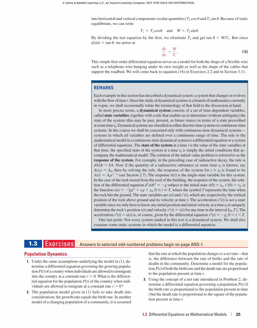
1.3 Differential Equations as Mathematical Models | 25
into horizontal and vertical components (scalar quantities) T2 cos u and T2 sin u. Because of static
equilibrium, we can write
T1 � T2 cos u and W � T2 sin u.
By dividing the last equation by the first, we eliminate T2 and get tan u � W/T1. But since
dy/dx � tan u, we arrive at
dy
dx�
W
T1
. (16)
This simple first-order differential equation serves as a model for both the shape of a flexible wire
such as a telephone wire hanging under its own weight as well as the shape of the cables that
support the roadbed. We will come back to equation (16) in Exercises 2.2 and in Section 3.11.
REMARKS
Each example in this section has described a dynamical system: a system that changes or evolves
with the flow of time t. Since the study of dynamical systems is a branch of mathematics currently
in vogue, we shall occasionally relate the terminology of that field to the discussion at hand.
In more precise terms, a dynamical system consists of a set of time-dependent variables,
called state variables, together with a rule that enables us to determine (without ambiguity) the
state of the system (this may be past, present, or future states) in terms of a state prescribed
at some time t0. Dynamical systems are classified as either discrete-time systems or continuous-time
systems. In this course we shall be concerned only with continuous-time dynamical systems—
systems in which all variables are defined over a continuous range of time. The rule or the
mathematical model in a continuous-time dynamical system is a differential equation or a system
of differential equations. The state of the system at a time t is the value of the state variables at
that time; the specified state of the system at a time t0 is simply the initial conditions that ac-
company the mathematical model. The solution of the initial-value problem is referred to as the
response of the system. For example, in the preceding case of radioactive decay, the rule is
dA/dt � kA. Now if the quantity of a radioactive substance at some time t0 is known, say
A(t0) � A0, then by solving the rule, the response of the system for t � t0 is found to be
A(t) � A0et2 t0 (see Section 2.7). The response A(t) is the single-state variable for this system.
In the case of the rock tossed from the roof of the building, the response of the system, the solu-
tion of the differential equation d 2s/dt 2 � �g subject to the initial state s(0) � s0, s�(0) � v0, is
the function s(t) � �12gt 2 � v0t � s0, 0 � t � T, where the symbol T represents the time when
the rock hits the ground. The state variables are s(t) and s�(t), which are, respectively, the vertical
position of the rock above ground and its velocity at time t. The acceleration s�(t) is not a state
variable since we only have to know any initial position and initial velocity at a time t0 to uniquely
determine the rock’s position s(t) and velocity s�(t) � v(t) for any time in the interval [t0, T ]. The
acceleration s�(t) � a(t) is, of course, given by the differential equation s�(t) � �g, 0 t T.One last point: Not every system studied in this text is a dynamical system. We shall also
examine some static systems in which the model is a differential equation.
Population Dynamics 1. Under the same assumptions underlying the model in (1), de-
termine a differential equation governing the growing popula-
tion P(t) of a country when individuals are allowed to immigrate
into the country at a constant rate r 0. What is the differen-
tial equation for the population P(t) of the country when indi-
viduals are allowed to emigrate at a constant rate r 0?
2. The population model given in (1) fails to take death into
consideration; the growth rate equals the birth rate. In another
model of a changing population of a community, it is assumed
that the rate at which the population changes is a net rate—that
is, the difference between the rate of births and the rate of
deaths in the community. Determine a model for the popula-
tion P(t) if both the birth rate and the death rate are proportional
to the population present at time t.
3. Using the concept of a net rate introduced in Problem 2, de-
termine a differential equation governing a population P(t) if the birth rate is proportional to the population present at time
t but the death rate is proportional to the square of the popula-
tion present at time t.
Exercises Answers to selected odd-numbered problems begin on page ANS-1.1.3
58229_CH01_001_031.indd Page 25 6/28/16 11:17 PM F-0017 58229_CH01_001_031.indd Page 25 6/28/16 11:17 PM F-0017 /202/JB00127/work/indd/202/JB00127/work/indd
© Jones & Bartlett Learning LLC, an Ascend Learning Company. NOT FOR SALE OR DISTRIBUTION.
© Jones & Bartlett Learning, LLCNOT FOR SALE OR DISTRIBUTION
© Jones & Bartlett Learning, LLCNOT FOR SALE OR DISTRIBUTION
© Jones & Bartlett Learning, LLCNOT FOR SALE OR DISTRIBUTION
© Jones & Bartlett Learning, LLCNOT FOR SALE OR DISTRIBUTION
© Jones & Bartlett Learning, LLCNOT FOR SALE OR DISTRIBUTION
© Jones & Bartlett Learning, LLCNOT FOR SALE OR DISTRIBUTION
© Jones & Bartlett Learning, LLCNOT FOR SALE OR DISTRIBUTION
© Jones & Bartlett Learning, LLCNOT FOR SALE OR DISTRIBUTION
© Jones & Bartlett Learning, LLCNOT FOR SALE OR DISTRIBUTION
© Jones & Bartlett Learning, LLCNOT FOR SALE OR DISTRIBUTION
© Jones & Bartlett Learning, LLCNOT FOR SALE OR DISTRIBUTION
© Jones & Bartlett Learning, LLCNOT FOR SALE OR DISTRIBUTION
© Jones & Bartlett Learning, LLCNOT FOR SALE OR DISTRIBUTION
© Jones & Bartlett Learning, LLCNOT FOR SALE OR DISTRIBUTION
© Jones & Bartlett Learning, LLCNOT FOR SALE OR DISTRIBUTION
© Jones & Bartlett Learning, LLCNOT FOR SALE OR DISTRIBUTION
© Jones & Bartlett Learning, LLCNOT FOR SALE OR DISTRIBUTION
© Jones & Bartlett Learning, LLCNOT FOR SALE OR DISTRIBUTION
© Jones & Bartlett Learning, LLCNOT FOR SALE OR DISTRIBUTION
© Jones & Bartlett Learning, LLCNOT FOR SALE OR DISTRIBUTION
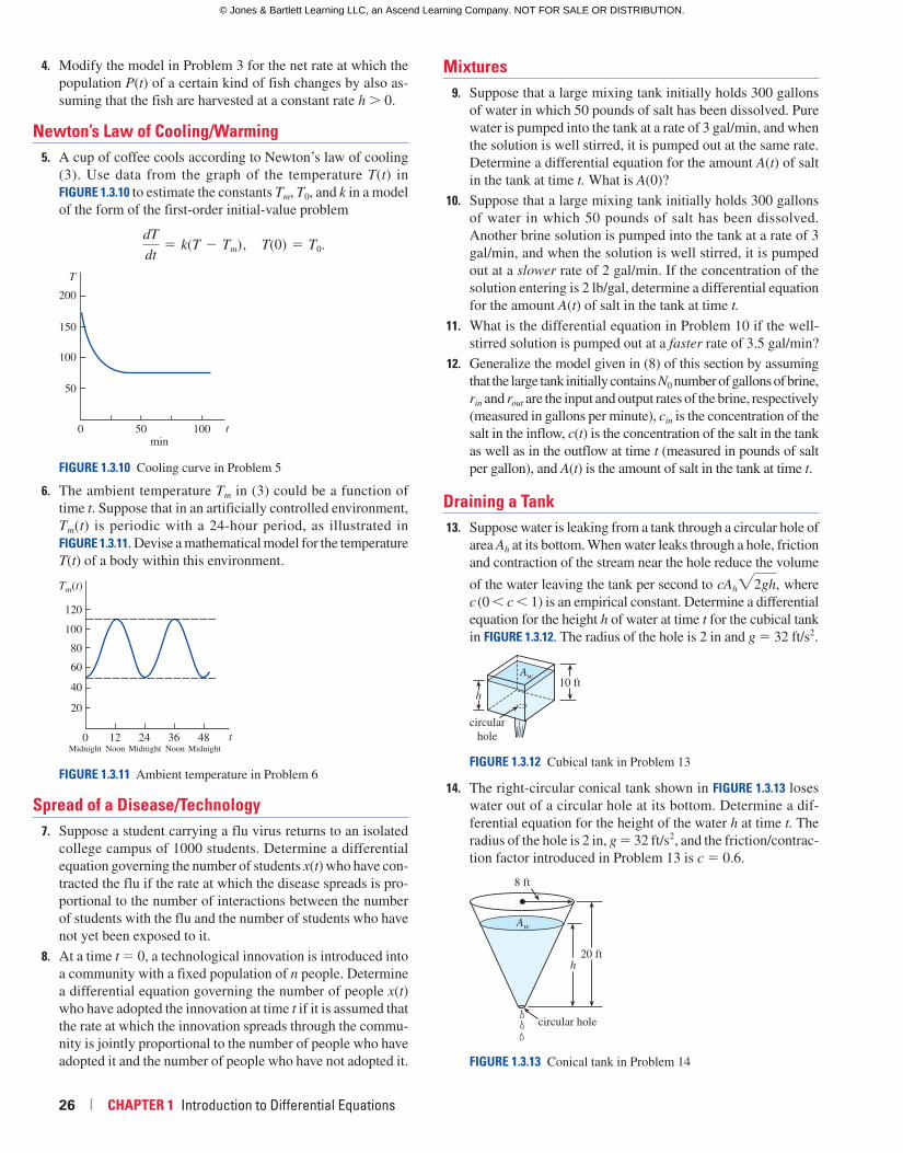
26 | CHAPTER 1 Introduction to Differential Equations
4. Modify the model in Problem 3 for the net rate at which the
population P(t) of a certain kind of fish changes by also as-
suming that the fish are harvested at a constant rate h � 0.
Newton’s Law of Cooling/Warming 5. A cup of coffee cools according to Newton’s law of cooling
(3). Use data from the graph of the temperature T(t) in
FIGURE 1.3.10 to estimate the constants Tm, T0, and k in a model
of the form of the first-order initial-value problem
dT
dt� k(T 2 Tm), T(0) � T0.
FIGURE 1.3.10 Cooling curve in Problem 5
200
150
100
50
T
0 50 100 tmin
6. The ambient temperature Tm in (3) could be a function of
time t. Suppose that in an artificially controlled environment,
Tm(t) is periodic with a 24-hour period, as illustrated in
FIGURE 1.3.11. Devise a mathematical model for the temperature
T(t) of a body within this environment.
FIGURE 1.3.11 Ambient temperature in Problem 6
100120
80604020
0 12 24 36 48 t
Tm(t)
Midnight Noon Midnight Noon Midnight
Spread of a Disease/Technology 7. Suppose a student carrying a flu virus returns to an isolated
college campus of 1000 students. Determine a differential
equation governing the number of students x(t) who have con-
tracted the flu if the rate at which the disease spreads is pro-
portional to the number of interactions between the number
of students with the flu and the number of students who have
not yet been exposed to it.
8. At a time t � 0, a technological innovation is introduced into
a community with a fixed population of n people. Determine
a differential equation governing the number of people x(t) who have adopted the innovation at time t if it is assumed that
the rate at which the innovation spreads through the commu-
nity is jointly proportional to the number of people who have
adopted it and the number of people who have not adopted it.
Mixtures 9. Suppose that a large mixing tank initially holds 300 gallons
of water in which 50 pounds of salt has been dissolved. Pure
water is pumped into the tank at a rate of 3 gal/min, and when
the solution is well stirred, it is pumped out at the same rate.
Determine a differential equation for the amount A(t) of salt
in the tank at time t. What is A(0)?
10. Suppose that a large mixing tank initially holds 300 gallons
of water in which 50 pounds of salt has been dissolved.
Another brine solution is pumped into the tank at a rate of 3
gal/min, and when the solution is well stirred, it is pumped
out at a slower rate of 2 gal/min. If the concentration of the
solution entering is 2 lb/gal, determine a differential equation
for the amount A(t) of salt in the tank at time t.
11. What is the differential equation in Problem 10 if the well-
stirred solution is pumped out at a faster rate of 3.5 gal/min?
12. Generalize the model given in (8) of this section by assuming
that the large tank initially contains N0 number of gallons of brine,
rin and rout are the input and output rates of the brine, respectively
(measured in gallons per minute), cin is the concentration of the
salt in the inflow, c(t) is the concentration of the salt in the tank
as well as in the outflow at time t (measured in pounds of salt
per gallon), and A(t) is the amount of salt in the tank at time t.
Draining a Tank 13. Suppose water is leaking from a tank through a circular hole of
area Ah at its bottom. When water leaks through a hole, friction
and contraction of the stream near the hole reduce the volume
of the water leaving the tank per second to cAh"2gh, where
c (0 c 1) is an empirical constant. Determine a differential
equation for the height h of water at time t for the cubical tank
in FIGURE 1.3.12. The radius of the hole is 2 in and g � 32 ft/s2.
FIGURE 1.3.12 Cubical tank in Problem 13
h10 ft
circularhole
Aw
14. The right-circular conical tank shown in FIGURE 1.3.13 loses
water out of a circular hole at its bottom. Determine a dif-
ferential equation for the height of the water h at time t. The
radius of the hole is 2 in, g � 32 ft/s2, and the friction/contrac-
tion factor introduced in Problem 13 is c � 0.6.
FIGURE 1.3.13 Conical tank in Problem 14
h20 ft
Aw
8 ft
circular hole
58229_CH01_001_031.indd Page 26 3/15/16 7:09 PM F-0017 58229_CH01_001_031.indd Page 26 3/15/16 7:09 PM F-0017 /202/JB00127/work/indd/202/JB00127/work/indd
© Jones & Bartlett Learning LLC, an Ascend Learning Company. NOT FOR SALE OR DISTRIBUTION.
© Jones & Bartlett Learning, LLCNOT FOR SALE OR DISTRIBUTION
© Jones & Bartlett Learning, LLCNOT FOR SALE OR DISTRIBUTION
© Jones & Bartlett Learning, LLCNOT FOR SALE OR DISTRIBUTION
© Jones & Bartlett Learning, LLCNOT FOR SALE OR DISTRIBUTION
© Jones & Bartlett Learning, LLCNOT FOR SALE OR DISTRIBUTION
© Jones & Bartlett Learning, LLCNOT FOR SALE OR DISTRIBUTION
© Jones & Bartlett Learning, LLCNOT FOR SALE OR DISTRIBUTION
© Jones & Bartlett Learning, LLCNOT FOR SALE OR DISTRIBUTION
© Jones & Bartlett Learning, LLCNOT FOR SALE OR DISTRIBUTION
© Jones & Bartlett Learning, LLCNOT FOR SALE OR DISTRIBUTION
© Jones & Bartlett Learning, LLCNOT FOR SALE OR DISTRIBUTION
© Jones & Bartlett Learning, LLCNOT FOR SALE OR DISTRIBUTION
© Jones & Bartlett Learning, LLCNOT FOR SALE OR DISTRIBUTION
© Jones & Bartlett Learning, LLCNOT FOR SALE OR DISTRIBUTION
© Jones & Bartlett Learning, LLCNOT FOR SALE OR DISTRIBUTION
© Jones & Bartlett Learning, LLCNOT FOR SALE OR DISTRIBUTION
© Jones & Bartlett Learning, LLCNOT FOR SALE OR DISTRIBUTION
© Jones & Bartlett Learning, LLCNOT FOR SALE OR DISTRIBUTION
© Jones & Bartlett Learning, LLCNOT FOR SALE OR DISTRIBUTION
© Jones & Bartlett Learning, LLCNOT FOR SALE OR DISTRIBUTION
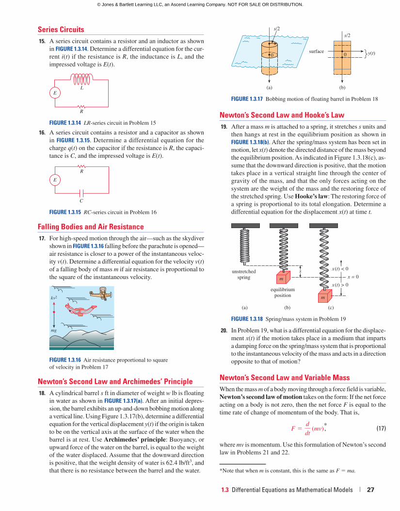
1.3 Differential Equations as Mathematical Models | 27
Series Circuits 15. A series circuit contains a resistor and an inductor as shown
in FIGURE 1.3.14. Determine a differential equation for the cur-
rent i(t) if the resistance is R, the inductance is L, and the
impressed voltage is E(t).
FIGURE 1.3.14 LR-series circuit in Problem 15
R
LE
16. A series circuit contains a resistor and a capacitor as shown
in FIGURE 1.3.15. Determine a differential equation for the
charge q(t) on the capacitor if the resistance is R, the capaci-
tance is C, and the impressed voltage is E(t).
FIGURE 1.3.15 RC-series circuit in Problem 16
C
RE
Falling Bodies and Air Resistance 17. For high-speed motion through the air—such as the skydiver
shown in FIGURE 1.3.16 falling before the parachute is opened—
air resistance is closer to a power of the instantaneous veloc-
ity v(t). Determine a differential equation for the velocity v(t) of a falling body of mass m if air resistance is proportional to
the square of the instantaneous velocity.
FIGURE 1.3.16 Air resistance proportional to square
of velocity in Problem 17
mg
kv2
Newton’s Second Law and Archimedes’ Principle 18. A cylindrical barrel s ft in diameter of weight w lb is floating
in water as shown in FIGURE 1.3.17(a). After an initial depres-
sion, the barrel exhibits an up-and-down bobbing motion along
a vertical line. Using Figure 1.3.17(b), determine a differential
equation for the vertical displacement y(t) if the origin is taken
to be on the vertical axis at the surface of the water when the
barrel is at rest. Use Archimedes’ principle: Buoyancy, or
upward force of the water on the barrel, is equal to the weight
of the water displaced. Assume that the downward direction
is positive, that the weight density of water is 62.4 lb/ft3, and
that there is no resistance between the barrel and the water.
FIGURE 1.3.17 Bobbing motion of floating barrel in Problem 18
s/2
0
(a)
surface
s/2
0
(b)
y(t)
Newton’s Second Law and Hooke’s Law 19. After a mass m is attached to a spring, it stretches s units and
then hangs at rest in the equilibrium position as shown in
FIGURE 1.3.18(b). After the spring/mass system has been set in
motion, let x(t) denote the directed distance of the mass beyond
the equilibrium position. As indicated in Figure 1.3.18(c), as-
sume that the downward direction is positive, that the motion
takes place in a vertical straight line through the center of
gravity of the mass, and that the only forces acting on the
system are the weight of the mass and the restoring force of
the stretched spring. Use Hooke’s law: The restoring force of
a spring is proportional to its total elongation. Determine a
differential equation for the displacement x(t) at time t.
FIGURE 1.3.18 Spring/mass system in Problem 19
m
m x = 0 s
(c)(b)
equilibriumposition
(a)
unstretchedspring
x (t) < 0
x (t) > 0
20. In Problem 19, what is a differential equation for the displace-
ment x(t) if the motion takes place in a medium that imparts
a damping force on the spring/mass system that is proportional
to the instantaneous velocity of the mass and acts in a direction
opposite to that of motion?
Newton’s Second Law and Variable MassWhen the mass m of a body moving through a force field is variable,
Newton’s second law of motion takes on the form: If the net force
acting on a body is not zero, then the net force F is equal to the
time rate of change of momentum of the body. That is,
F �d
dt (mv)
*, (17)
where mv is momentum. Use this formulation of Newton’s second
law in Problems 21 and 22.
*Note that when m is constant, this is the same as F � ma.
58229_CH01_001_031.indd Page 27 6/18/16 5:51 AM F-0017 58229_CH01_001_031.indd Page 27 6/18/16 5:51 AM F-0017 /202/JB00127/work/indd/202/JB00127/work/indd
© Jones & Bartlett Learning LLC, an Ascend Learning Company. NOT FOR SALE OR DISTRIBUTION.
© Jones & Bartlett Learning, LLCNOT FOR SALE OR DISTRIBUTION
© Jones & Bartlett Learning, LLCNOT FOR SALE OR DISTRIBUTION
© Jones & Bartlett Learning, LLCNOT FOR SALE OR DISTRIBUTION
© Jones & Bartlett Learning, LLCNOT FOR SALE OR DISTRIBUTION
© Jones & Bartlett Learning, LLCNOT FOR SALE OR DISTRIBUTION
© Jones & Bartlett Learning, LLCNOT FOR SALE OR DISTRIBUTION
© Jones & Bartlett Learning, LLCNOT FOR SALE OR DISTRIBUTION
© Jones & Bartlett Learning, LLCNOT FOR SALE OR DISTRIBUTION
© Jones & Bartlett Learning, LLCNOT FOR SALE OR DISTRIBUTION
© Jones & Bartlett Learning, LLCNOT FOR SALE OR DISTRIBUTION
© Jones & Bartlett Learning, LLCNOT FOR SALE OR DISTRIBUTION
© Jones & Bartlett Learning, LLCNOT FOR SALE OR DISTRIBUTION
© Jones & Bartlett Learning, LLCNOT FOR SALE OR DISTRIBUTION
© Jones & Bartlett Learning, LLCNOT FOR SALE OR DISTRIBUTION
© Jones & Bartlett Learning, LLCNOT FOR SALE OR DISTRIBUTION
© Jones & Bartlett Learning, LLCNOT FOR SALE OR DISTRIBUTION
© Jones & Bartlett Learning, LLCNOT FOR SALE OR DISTRIBUTION
© Jones & Bartlett Learning, LLCNOT FOR SALE OR DISTRIBUTION
© Jones & Bartlett Learning, LLCNOT FOR SALE OR DISTRIBUTION
© Jones & Bartlett Learning, LLCNOT FOR SALE OR DISTRIBUTION
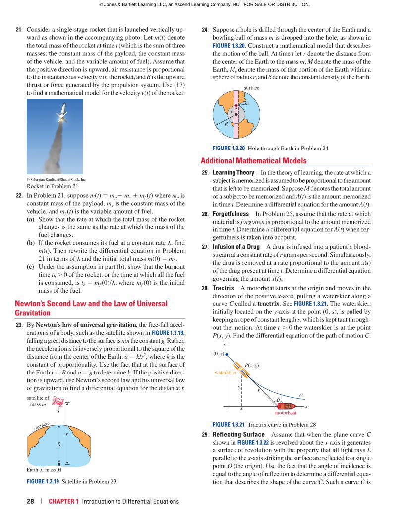
28 | CHAPTER 1 Introduction to Differential Equations
21. Consider a single-stage rocket that is launched vertically up-
ward as shown in the accompanying photo. Let m(t) denote
the total mass of the rocket at time t (which is the sum of three
masses: the constant mass of the payload, the constant mass
of the vehicle, and the variable amount of fuel). Assume that
the positive direction is upward, air resistance is proportional
to the instantaneous velocity v of the rocket, and R is the upward
thrust or force generated by the propulsion system. Use (17)
to find a mathematical model for the velocity v(t) of the rocket.
© Sebastian Kaulitzki/ShutterStock, Inc.
Rocket in Problem 21
22. In Problem 21, suppose m(t) � mp � mv � mf (t) where mp is
constant mass of the payload, mv is the constant mass of the
vehicle, and mf (t) is the variable amount of fuel.
(a) Show that the rate at which the total mass of the rocket
changes is the same as the rate at which the mass of the
fuel changes.
(b) If the rocket consumes its fuel at a constant rate l, find
m(t). Then rewrite the differential equation in Problem
21 in terms of l and the initial total mass m(0) � m0.
(c) Under the assumption in part (b), show that the burnout
time tb � 0 of the rocket, or the time at which all the fuel
is consumed, is tb � mf (0)/l, where mf (0) is the initial
mass of the fuel.
Newton’s Second Law and the Law of Universal Gravitation 23. By Newton’s law of universal gravitation, the free-fall accel-
eration a of a body, such as the satellite shown in FIGURE 1.3.19,
falling a great distance to the surface is not the constant g. Rather,
the acceleration a is inversely proportional to the square of the
distance from the center of the Earth, a � k/r2, where k is the
constant of proportionality. Use the fact that at the surface of
the Earth r � R and a � g to determine k. If the positive direc-
tion is upward, use Newton’s second law and his universal law
of gravitation to find a differential equation for the distance r.
FIGURE 1.3.19 Satellite in Problem 23
satellite ofmass m
Earth of mass M
Rr
surface
24. Suppose a hole is drilled through the center of the Earth and a
bowling ball of mass m is dropped into the hole, as shown in
FIGURE 1.3.20. Construct a mathematical model that describes
the motion of the ball. At time t let r denote the distance from
the center of the Earth to the mass m, M denote the mass of the
Earth, Mr denote the mass of that portion of the Earth within a
sphere of radius r, and d denote the constant density of the Earth.
FIGURE 1.3.20 Hole through Earth in Problem 24
m
R
r
surface
Additional Mathematical Models 25. Learning Theory In the theory of learning, the rate at which a
subject is memorized is assumed to be proportional to the amount
that is left to be memorized. Suppose M denotes the total amount
of a subject to be memorized and A(t) is the amount memorized
in time t. Determine a differential equation for the amount A(t).
26. Forgetfulness In Problem 25, assume that the rate at which
material is forgotten is proportional to the amount memorized
in time t. Determine a differential equation for A(t) when for-
getfulness is taken into account.
27. Infusion of a Drug A drug is infused into a patient’s blood-
stream at a constant rate of r grams per second. Simultaneously,
the drug is removed at a rate proportional to the amount x(t) of the drug present at time t. Determine a differential equation
governing the amount x(t).
28. Tractrix A motorboat starts at the origin and moves in the
direction of the positive x-axis, pulling a waterskier along a
curve C called a tractrix. See FIGURE 1.3.21. The waterskier,
initially located on the y-axis at the point (0, s), is pulled by
keeping a rope of constant length s, which is kept taut through-
out the motion. At time t . 0 the waterskier is at the point
P(x, y). Find the differential equation of the path of motion C.
FIGURE 1.3.21 Tractrix curve in Problem 28
C
y
y s
P(x, y)
(0, s)
motorboatxx
waterskier
θ
29. Reflecting Surface Assume that when the plane curve C
shown in FIGURE 1.3.22 is revolved about the x-axis it generates
a surface of revolution with the property that all light rays L
parallel to the x-axis striking the surface are reflected to a single
point O (the origin). Use the fact that the angle of incidence is
equal to the angle of reflection to determine a differential equa-
tion that describes the shape of the curve C. Such a curve C is
58229_CH01_001_031.indd Page 28 6/6/16 3:28 PM F-0017 58229_CH01_001_031.indd Page 28 6/6/16 3:28 PM F-0017 /202/JB00127/work/indd/202/JB00127/work/indd
© Jones & Bartlett Learning LLC, an Ascend Learning Company. NOT FOR SALE OR DISTRIBUTION.
© Jones & Bartlett Learning, LLCNOT FOR SALE OR DISTRIBUTION
© Jones & Bartlett Learning, LLCNOT FOR SALE OR DISTRIBUTION
© Jones & Bartlett Learning, LLCNOT FOR SALE OR DISTRIBUTION
© Jones & Bartlett Learning, LLCNOT FOR SALE OR DISTRIBUTION
© Jones & Bartlett Learning, LLCNOT FOR SALE OR DISTRIBUTION
© Jones & Bartlett Learning, LLCNOT FOR SALE OR DISTRIBUTION
© Jones & Bartlett Learning, LLCNOT FOR SALE OR DISTRIBUTION
© Jones & Bartlett Learning, LLCNOT FOR SALE OR DISTRIBUTION
© Jones & Bartlett Learning, LLCNOT FOR SALE OR DISTRIBUTION
© Jones & Bartlett Learning, LLCNOT FOR SALE OR DISTRIBUTION
© Jones & Bartlett Learning, LLCNOT FOR SALE OR DISTRIBUTION
© Jones & Bartlett Learning, LLCNOT FOR SALE OR DISTRIBUTION
© Jones & Bartlett Learning, LLCNOT FOR SALE OR DISTRIBUTION
© Jones & Bartlett Learning, LLCNOT FOR SALE OR DISTRIBUTION
© Jones & Bartlett Learning, LLCNOT FOR SALE OR DISTRIBUTION
© Jones & Bartlett Learning, LLCNOT FOR SALE OR DISTRIBUTION
© Jones & Bartlett Learning, LLCNOT FOR SALE OR DISTRIBUTION
© Jones & Bartlett Learning, LLCNOT FOR SALE OR DISTRIBUTION
© Jones & Bartlett Learning, LLCNOT FOR SALE OR DISTRIBUTION
© Jones & Bartlett Learning, LLCNOT FOR SALE OR DISTRIBUTION

1.3 Differential Equations as Mathematical Models | 29
important in applications ranging from construction of telescopes
to satellite antennas, automobile headlights, and solar collectors.
[Hint: Inspection of the figure shows that we can write f � 2u.
Why? Now use an appropriate trigonometric identity.]
C
θ
θ
L
O x
y tangent
φ
P(x, y)
FIGURE 1.3.22 Reflecting surface in Problem 29
Discussion Problems 30. Reread Problem 45 in Exercises 1.1 and then give an explicit
solution P(t) for equation (1). Find a one-parameter family of
solutions of (1).
31. Reread the sentence following equation (3) and assume that
Tm is a positive constant. Discuss why we would expect
k � 0 in (3) in both cases of cooling and warming. You might
start by interpreting, say, T(t) � Tm in a graphical manner.
32. Reread the discussion leading up to equation (8). If we assume
that initially the tank holds, say, 50 lbs of salt, it stands to reason
that since salt is being added to the tank continuously for t � 0,
that A(t) should be an increasing function. Discuss how you
might determine from the DE, without actually solving it, the
number of pounds of salt in the tank after a long period of time.
33. Population Model The differential equation dP/dt � (k cos t)P,
where k is a positive constant, is a model of human population
P(t) of a certain community. Discuss an interpretation for the
solution of this equation; in other words, what kind of popu-
lation do you think the differential equation describes?
34. Rotating Fluid As shown in FIGURE 1.3.23(a), a right-circular
cylinder partially filled with fluid is rotated with a constant
angular velocity v about a vertical y-axis through its center. The
rotating fluid is a surface of revolution S. To identify S we first
establish a coordinate system consisting of a vertical plane de-
termined by the y-axis and an x-axis drawn perpendicular to the
y-axis such that the point of intersection of the axes (the origin)
is located at the lowest point on the surface S. We then seek a
function y � f (x), which represents the curve C of intersection
of the surface S and the vertical coordinate plane. Let the point
P(x, y) denote the position of a particle of the rotating fluid of
mass m in the coordinate plane. See Figure 1.3.23(b).
(a) At P, there is a reaction force of magnitude F due to the
other particles of the fluid, which is normal to the surface S.
By Newton’s second law the magnitude of the net force
acting on the particle is mv2x. What is this force? Use Figure
1.3.23(b) to discuss the nature and origin of the equations
F cos u � mg, F sin u � mv2x.
(b) Use part (a) to find a first-order differential equation that
defines the function y � f (x).
FIGURE 1.3.23 Rotating fluid in Problem 34
θ
θ mg
x
y
P(x, y)
tangent line tocurve C at P
curve C of intersectionof xy-plane andsurface of revolution
mw 2x
yw
P
(a) (b)
35. Falling Body In Problem 23, suppose r � R � s, where s is
the distance from the surface of the Earth to the falling body.
What does the differential equation obtained in Problem 23
become when s is very small compared to R?
36. Raindrops Keep Falling In meteorology, the term virga refers
to falling raindrops or ice particles that evaporate before they
reach the ground. Assume that a typical raindrop is spherical
in shape. Starting at some time, which we can designate as
t � 0, the raindrop of radius r0 falls from rest from a cloud
and begins to evaporate.
(a) If it is assumed that a raindrop evaporates in such a manner
that its shape remains spherical, then it also makes sense to
assume that the rate at which the raindrop evaporates—that
is, the rate at which it loses mass—is proportional to its
surface area. Show that this latter assumption implies that
the rate at which the radius r of the raindrop decreases is
a constant. Find r(t). [Hint: See Problem 55 in Exercises 1.1.]
(b) If the positive direction is downward, construct a math-
ematical model for the velocity v of the falling raindrop
at time t. Ignore air resistance. [Hint: Use the form of
Newton’s second law as given in (17).]
37. Let It Snow The “snowplow problem” is a classic and appears
in many differential equations texts but was probably made
famous by Ralph Palmer Agnew:
“One day it started snowing at a heavy and steady rate. A snowplow started out at noon, going 2 miles the first hour and 1 mile the second hour. What time did it start snowing?”
If possible, find the text Differential Equations, Ralph Palmer
Agnew, McGraw-Hill, and then discuss the construction and
solution of the mathematical model.
© aetb/iStock/Thinkstock
Snowplow in Problem 37
58229_CH01_001_031.indd Page 29 6/6/16 3:27 PM F-0017 58229_CH01_001_031.indd Page 29 6/6/16 3:27 PM F-0017 /202/JB00127/work/indd/202/JB00127/work/indd
© Jones & Bartlett Learning LLC, an Ascend Learning Company. NOT FOR SALE OR DISTRIBUTION.
© Jones & Bartlett Learning, LLCNOT FOR SALE OR DISTRIBUTION
© Jones & Bartlett Learning, LLCNOT FOR SALE OR DISTRIBUTION
© Jones & Bartlett Learning, LLCNOT FOR SALE OR DISTRIBUTION
© Jones & Bartlett Learning, LLCNOT FOR SALE OR DISTRIBUTION
© Jones & Bartlett Learning, LLCNOT FOR SALE OR DISTRIBUTION
© Jones & Bartlett Learning, LLCNOT FOR SALE OR DISTRIBUTION
© Jones & Bartlett Learning, LLCNOT FOR SALE OR DISTRIBUTION
© Jones & Bartlett Learning, LLCNOT FOR SALE OR DISTRIBUTION
© Jones & Bartlett Learning, LLCNOT FOR SALE OR DISTRIBUTION
© Jones & Bartlett Learning, LLCNOT FOR SALE OR DISTRIBUTION
© Jones & Bartlett Learning, LLCNOT FOR SALE OR DISTRIBUTION
© Jones & Bartlett Learning, LLCNOT FOR SALE OR DISTRIBUTION
© Jones & Bartlett Learning, LLCNOT FOR SALE OR DISTRIBUTION
© Jones & Bartlett Learning, LLCNOT FOR SALE OR DISTRIBUTION
© Jones & Bartlett Learning, LLCNOT FOR SALE OR DISTRIBUTION
© Jones & Bartlett Learning, LLCNOT FOR SALE OR DISTRIBUTION
© Jones & Bartlett Learning, LLCNOT FOR SALE OR DISTRIBUTION
© Jones & Bartlett Learning, LLCNOT FOR SALE OR DISTRIBUTION
© Jones & Bartlett Learning, LLCNOT FOR SALE OR DISTRIBUTION
© Jones & Bartlett Learning, LLCNOT FOR SALE OR DISTRIBUTION
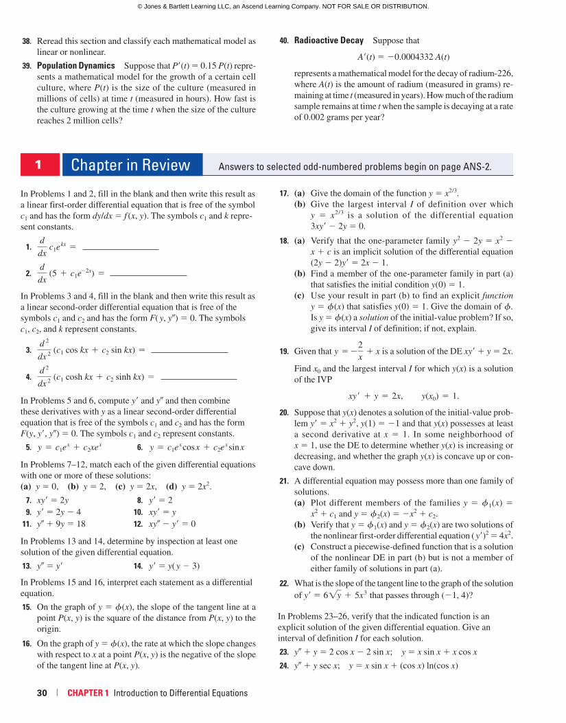
30 | CHAPTER 1 Introduction to Differential Equations
38. Reread this section and classify each mathematical model as
linear or nonlinear.
39. Population Dynamics Suppose that P�(t) � 0.15 P(t) repre-
sents a mathematical model for the growth of a certain cell
culture, where P(t) is the size of the culture (measured in
millions of cells) at time t (measured in hours). How fast is
the culture growing at the time t when the size of the culture
reaches 2 million cells?
40. Radioactive Decay Suppose that
A�(t) � �0.0004332 A(t)
represents a mathematical model for the decay of radium-226,
where A(t) is the amount of radium (measured in grams) re-
maining at time t (measured in years). How much of the radium
sample remains at time t when the sample is decaying at a rate
of 0.002 grams per year?
In Problems 1 and 2, fill in the blank and then write this result as
a linear first-order differential equation that is free of the symbol
c1 and has the form dy/dx � f (x, y). The symbols c1 and k repre-
sent constants.
1. d
dx c1e
kx �
2. d
dx (5 � c1e
�2x) �
In Problems 3 and 4, fill in the blank and then write this result as
a linear second-order differential equation that is free of the
symbols c1 and c2 and has the form F( y, y�) � 0. The symbols
c1, c2, and k represent constants.
3. d 2
dx 2 (c1 cos kx � c2 sin kx) �
4. d 2
dx 2 (c1 cosh kx � c2 sinh kx) �
In Problems 5 and 6, compute y� and y� and then combine
these derivatives with y as a linear second-order differential
equation that is free of the symbols c1 and c2 and has the form
F(y, y�, y�) � 0. The symbols c1 and c2 represent constants.
5. y � c1ex � c2xex 6. y � c1e
x cos x � c2e
x sin x
In Problems 7–12, match each of the given differential equations
with one or more of these solutions:
(a) y � 0, (b) y � 2, (c) y � 2x, (d) y � 2x2.
7. xy� � 2y 8. y� � 2
9. y� � 2y � 4 10. xy� � y 11. y� � 9y � 18 12. xy� � y� � 0
In Problems 13 and 14, determine by inspection at least one
solution of the given differential equation.
13. y� � y� 14. y� � y( y � 3)
In Problems 15 and 16, interpret each statement as a differential
equation.
15. On the graph of y � f(x), the slope of the tangent line at a
point P(x, y) is the square of the distance from P(x, y) to the
origin.
16. On the graph of y � f(x), the rate at which the slope changes
with respect to x at a point P(x, y) is the negative of the slope
of the tangent line at P(x, y).
17. (a) Give the domain of the function y � x2/3.
(b) Give the largest interval I of definition over which
y � x2/3 is a solution of the differential equation
3xy� � 2y � 0.
18. (a) Verify that the one-parameter family y2 � 2y � x2 �
x � c is an implicit solution of the differential equation
(2y � 2)y� � 2x � 1.
(b) Find a member of the one-parameter family in part (a)
that satisfies the initial condition y(0) � 1.
(c) Use your result in part (b) to find an explicit function
y � f(x) that satisfies y(0) � 1. Give the domain of f. Is y � f(x) a solution of the initial-value problem? If so,
give its interval I of definition; if not, explain.
19. Given that y � �2
x� x is a solution of the DE xy� � y � 2x.
Find x0 and the largest interval I for which y(x) is a solution
of the IVP
xy9 � y � 2x, y(x0) � 1.
20. Suppose that y(x) denotes a solution of the initial-value prob-
lem y� � x2 � y2, y(1) � �1 and that y(x) possesses at least
a second derivative at x � 1. In some neighborhood of
x � 1, use the DE to determine whether y(x) is increasing or
decreasing, and whether the graph y(x) is concave up or con-
cave down.
21. A differential equation may possess more than one family of
solutions.
(a) Plot different members of the families y � f1(x) �
x2 � c1 and y � f2(x) � �x2 � c2.
(b) Verify that y � f1(x) and y � f2(x) are two solutions of
the nonlinear first-order differential equation ( y�)2 � 4x2.
(c) Construct a piecewise-defined function that is a solution
of the nonlinear DE in part (b) but is not a member of
either family of solutions in part (a).
22. What is the slope of the tangent line to the graph of the solution
of y� � 6!y � 5x3 that passes through (�1, 4)?
In Problems 23–26, verify that the indicated function is an
explicit solution of the given differential equation. Give an
interval of definition I for each solution.
23. y� � y � 2 cos x � 2 sin x; y � x sin x � x cos x
24. y� � y sec x; y � x sin x � (cos x) ln(cos x)
1 Chapter in Review Answers to selected odd-numbered problems begin on page ANS-2.
58229_CH01_001_031.indd Page 30 6/28/16 11:18 PM F-0017 58229_CH01_001_031.indd Page 30 6/28/16 11:18 PM F-0017 /202/JB00127/work/indd/202/JB00127/work/indd
© Jones & Bartlett Learning LLC, an Ascend Learning Company. NOT FOR SALE OR DISTRIBUTION.
© Jones & Bartlett Learning, LLCNOT FOR SALE OR DISTRIBUTION
© Jones & Bartlett Learning, LLCNOT FOR SALE OR DISTRIBUTION
© Jones & Bartlett Learning, LLCNOT FOR SALE OR DISTRIBUTION
© Jones & Bartlett Learning, LLCNOT FOR SALE OR DISTRIBUTION
© Jones & Bartlett Learning, LLCNOT FOR SALE OR DISTRIBUTION
© Jones & Bartlett Learning, LLCNOT FOR SALE OR DISTRIBUTION
© Jones & Bartlett Learning, LLCNOT FOR SALE OR DISTRIBUTION
© Jones & Bartlett Learning, LLCNOT FOR SALE OR DISTRIBUTION
© Jones & Bartlett Learning, LLCNOT FOR SALE OR DISTRIBUTION
© Jones & Bartlett Learning, LLCNOT FOR SALE OR DISTRIBUTION
© Jones & Bartlett Learning, LLCNOT FOR SALE OR DISTRIBUTION
© Jones & Bartlett Learning, LLCNOT FOR SALE OR DISTRIBUTION
© Jones & Bartlett Learning, LLCNOT FOR SALE OR DISTRIBUTION
© Jones & Bartlett Learning, LLCNOT FOR SALE OR DISTRIBUTION
© Jones & Bartlett Learning, LLCNOT FOR SALE OR DISTRIBUTION
© Jones & Bartlett Learning, LLCNOT FOR SALE OR DISTRIBUTION
© Jones & Bartlett Learning, LLCNOT FOR SALE OR DISTRIBUTION
© Jones & Bartlett Learning, LLCNOT FOR SALE OR DISTRIBUTION
© Jones & Bartlett Learning, LLCNOT FOR SALE OR DISTRIBUTION
© Jones & Bartlett Learning, LLCNOT FOR SALE OR DISTRIBUTION
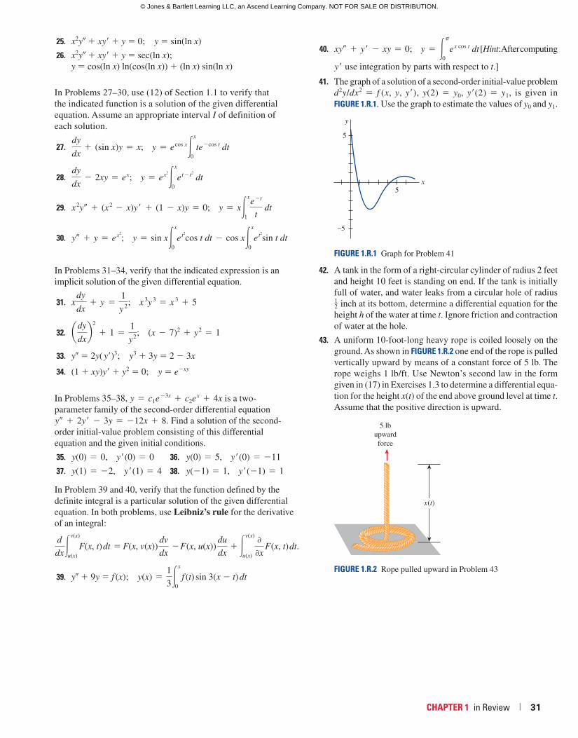
CHAPTER 1 in Review | 31
25. x2y� � xy� � y � 0; y � sin(ln x)
26. x2y� � xy� � y � sec(ln x);
y � cos(ln x) ln(cos(ln x)) � (ln x) sin(ln x)
In Problems 27–30, use (12) of Section 1.1 to verify that
the indicated function is a solution of the given differential
equation. Assume an appropriate interval I of definition of
each solution.
27. dy
dx� (sin x)y � x; y � ecos x#
x
0
te�cos t dt
28. dy
dx2 2xy � ex; y � ex2#
x
0
et2 t2
dt
29. x2y0 � (x2 2 x)y9 � (1 2 x)y � 0; y � x#x
1
e�t
t dt
30. y0 � y � ex2
; y � sin x#x
0
et2
cos t dt 2 cos x#x
0
et2
sin t dt
In Problems 31–34, verify that the indicated expression is an
implicit solution of the given differential equation.
31. xdy
dx� y �
1
y 2; x 3y 3 � x 3 � 5
32. ady
dxb2
� 1 �1
y2; (x 2 7)2 � y2 � 1
33. y� � 2y( y�)3; y3 � 3y � 2 � 3x
34. (1 � xy)y� � y2 � 0; y � e�xy
In Problems 35–38, y � c1e�3x � c2e
x � 4x is a two-
parameter family of the second-order differential equation
y0 � 2y9 2 3y � �12x � 8. Find a solution of the second-
order initial-value problem consisting of this differential
equation and the given initial conditions.
35. y(0) � 0, y9(0) � 0 36. y(0) � 5, y9(0) � �11
37. y(1) � �2, y9(1) � 4 38. y(�1) � 1, y9(�1) � 1
In Problem 39 and 40, verify that the function defined by the
definite integral is a particular solution of the given differential
equation. In both problems, use Leibniz’s rule for the derivative
of an integral:
d
dx#v(x)
u(x)
F(x, t) dt � F(x, v(x))
dv
dx2F(x, u(x))
du
dx� #
v(x)
u(x)
0
0x F(x, t) dt.
39. y� � 9y � f (x); y(x) �1
3#x
0
f (t) sin 3(x � t) dt
40. xy0 � y9 2 xy � 0; y � #p
0
ex cos t dt [Hint: After computing
y9 use integration by parts with respect to t.]
41. The graph of a solution of a second-order initial-value problem
d2y/dx2 � f (x, y, y�), y(2) � y0, y�(2) � y1, is given in
FIGURE 1.R.1. Use the graph to estimate the values of y0 and y1.
FIGURE 1.R.1 Graph for Problem 41
y
x
5
–5
5
42. A tank in the form of a right-circular cylinder of radius 2 feet
and height 10 feet is standing on end. If the tank is initially
full of water, and water leaks from a circular hole of radius 12 inch at its bottom, determine a differential equation for the
height h of the water at time t. Ignore friction and contraction
of water at the hole.
43. A uniform 10-foot-long heavy rope is coiled loosely on the
ground. As shown in FIGURE 1.R.2 one end of the rope is pulled
vertically upward by means of a constant force of 5 lb. The
rope weighs 1 lb/ft. Use Newton’s second law in the form
given in (17) in Exercises 1.3 to determine a differential equa-
tion for the height x(t) of the end above ground level at time t. Assume that the positive direction is upward.
FIGURE 1.R.2 Rope pulled upward in Problem 43
x(t)
5 lbupwardforce
58229_CH01_001_031.indd Page 31 5/24/16 6:50 PM f-500 58229_CH01_001_031.indd Page 31 5/24/16 6:50 PM f-500 /202/JB00127/work/indd/202/JB00127/work/indd
© Jones & Bartlett Learning LLC, an Ascend Learning Company. NOT FOR SALE OR DISTRIBUTION.
© Jones & Bartlett Learning, LLCNOT FOR SALE OR DISTRIBUTION
© Jones & Bartlett Learning, LLCNOT FOR SALE OR DISTRIBUTION
© Jones & Bartlett Learning, LLCNOT FOR SALE OR DISTRIBUTION
© Jones & Bartlett Learning, LLCNOT FOR SALE OR DISTRIBUTION
© Jones & Bartlett Learning, LLCNOT FOR SALE OR DISTRIBUTION
© Jones & Bartlett Learning, LLCNOT FOR SALE OR DISTRIBUTION
© Jones & Bartlett Learning, LLCNOT FOR SALE OR DISTRIBUTION
© Jones & Bartlett Learning, LLCNOT FOR SALE OR DISTRIBUTION
© Jones & Bartlett Learning, LLCNOT FOR SALE OR DISTRIBUTION
© Jones & Bartlett Learning, LLCNOT FOR SALE OR DISTRIBUTION
© Jones & Bartlett Learning, LLCNOT FOR SALE OR DISTRIBUTION
© Jones & Bartlett Learning, LLCNOT FOR SALE OR DISTRIBUTION
© Jones & Bartlett Learning, LLCNOT FOR SALE OR DISTRIBUTION
© Jones & Bartlett Learning, LLCNOT FOR SALE OR DISTRIBUTION
© Jones & Bartlett Learning, LLCNOT FOR SALE OR DISTRIBUTION
© Jones & Bartlett Learning, LLCNOT FOR SALE OR DISTRIBUTION
© Jones & Bartlett Learning, LLCNOT FOR SALE OR DISTRIBUTION
© Jones & Bartlett Learning, LLCNOT FOR SALE OR DISTRIBUTION
© Jones & Bartlett Learning, LLCNOT FOR SALE OR DISTRIBUTION
© Jones & Bartlett Learning, LLCNOT FOR SALE OR DISTRIBUTION