M. Sc. Differential Equations Mathematics Title.p65 - Shivaji ...
197
SHIVAJI UNIVERSITY, KOLHAPUR CENTRE FOR DISTANCE EDUCATION Differential Equations (Mathematics) For M. Sc. Part-I H I K J
-
Upload
khangminh22 -
Category
Documents
-
view
5 -
download
0
Transcript of M. Sc. Differential Equations Mathematics Title.p65 - Shivaji ...

SHIVAJI UNIVERSITY, KOLHAPUR
CENTRE FOR DISTANCE EDUCATION
Differential Equations(Mathematics)
For
M. Sc. Part-I
H I
K J

Copyright © Registrar,
Shivaji University,
Kolhapur. (Maharashtra)
First Edition 2008
Second Edition 2010
Prescribed for M. Sc. Part-I
All rights reserved, No part of this work may be reproduced in any form by mimeography or
any other means without permission in writing from the Shivaji University, Kolhapur (MS)
Copies : 1000
Published by:
Dr. D. V. Muley
Registrar,
Shivaji University,
Kolhapur-416 004
Printed by :
Shri. A. S. Mane,
I/c. Superintendent,
Shivaji University Press,
Kolhapur-416 004
ISBN- 978-81-8486-012-2
H Further information about the Centre for Distance Education & Shivaji University may be
obtained from the University Office at Vidyanagar, Kolhapur-416 004, India.
H This material has been produced with the developmental grant from DEC-IGNOU, New
Delhi.
(ii)

Prof. (Dr.) N. J. Pawar
Vice-Chancellor,
Shivaji University, Kolhapur
Centre for Distance Education
Shivaji University, Kolhapur
n EXPERT COMMITTEE n
Dr. D. V. Muley
Registrar,
Shivaji University, Kolhapur.
n ADVISORY COMMITTEE n
n B. O. S. MEMBERS OF MATHEMATICS n
Chairman- Prof. S. R. Bhosale
P.D.V.P. Mahavidyalaya, Tasgaon, Dist. Sangli.
l Dr. L. N. Katkar
Head, Dept. of Mathematics,
Shivaji University, Kolhapur.
l Dr. H. T. Dinde
Karmveer Bhaurao Patil College, Urun-Islampur,
Tal. Walwa, Dist. Sangli.
l Dr. T. B. Jagtap
Yashwantrao Chavan Institute of Science, Satara.
l Shri. L. B. Jamale
Krishna Mahavidyalaya, Rethare Bk., Karad,
Dist. Satara.
l Dr. A. D. Lokhande
Yashavantrao Chavan Warana Mahavidyalaya,
Warananagar.
l Prof. S. P. Patankar
Vivekanand College, Kolhapur.
l Prof. V. P. Rathod
Dept. of Mathematics, Gulbarga University,
Gulbarga, (Karnataka State.)
l Prof. S. S. Benchalli
Dept. of Mathematics,Karnataka University, Dharwad.
l Shri. Santosh Pawar,
1012, 'A' Ward Sadashiv Jadhav, Housing
Society, Radhanagari Road, Kolhapur-416 012.
Prof. (Dr.) N. J. Pawar
Vice-Chancellor,
Shivaji University, Kolhapur.
Dr. A. B. Rajge
Director BCUD,
Shivaji University, Kolhapur.
Dr. B. M. Hirdekar
Controller of Examination
Shivaji University, Kolhapur.
Dr. (Smt.) Vasanti Rasam
Dean, Faculty of Social Sciences,
Shivaji University, Kolhapur.
Prof. (Dr.) B. S. Sawant
Dean, Faculty of Commerce,
Shivaji University, Kolhapur.
Dr. T. B. Jagtap
Dean, Faculty of Science,
Shivaji University, Kolhapur.
Dr. K. N. Sangale
Dean, Faculty of Education,
Shivaji University, Kolhapur.
Dr. D. V. Muley
Registrar,
Shivaji University, Kolhapur.
Shri. B. S. Patil
Finance and Accounts Officer,
Shivaji University, Kolhapur.
Prof. (Dr.) U. B. Bhoite
Lal Bahadur Shastri Marg,
Bharati Vidyapeeth, Pune.
Prof. (Dr.) A. N. Joshi
Director, School of Education,
Y. C. M. O. U. Nashik.
Shri. J. R. Jadhav
Dean, Faculty of Arts & Fine Arts,
Shivaji University, Kolhapur.
Prof. (Dr.) S. A. Bari
Director, Distance Education,
Kuvempu University, Karnataka.
Prof. Dr. (Smt.) Cima Yeole
(Member Secretary)
Director, Centre for Distance Education,
Shivaji University, Kolhapur.
(iii)

Centre for Distance Education
Shivaji University,
Kolhapur.
Differential Equations
Writing Team
(iv)
Dr. (Mrs.) Sarita Thakar All
Department of Mathematics
Shivaji University, Kolhapur.
Maharashtra
Dr. (Mrs.) Sarita Thakar
Department of Mathematics,
Shivaji University, Kolhapur.
Maharashtra.
n Editor n
Unit No.

Preface
Large numbers of students appear for M.A./M. Sc. Examinations externally every
year. In view of this, Shivaji University has introduced the Distance Education Mode for
external students from the year 2007-2008, and entrusted the task to us to prepare the
Self Instructional Material (SIM) for aspirants.
It is hoped that students must learn Mathematics not only to become competent
mathematicians but also skilled users of Mathematics in the solution of problems in the
real world. They must learn how to use their Mathematical knowledge in solving the
problems of the real world. Differential equations usually are description of physical
systems. This book on Differential Equations consists of four chapters. Chapter one
contains the complete discussion of linear equations with constant coefficients, including
the uniqueness theorem. In chapter two linear equations with variable coefficients are
trea. Equations with analytic coefficients are introduced and series solutions are
obtained by a simple formal process. A detailed treatment of linear equations with
regular singular points is discussed in chapter four. Classification of regular singular
points and regular singular points at infinity is studied. In chapter five existence and
uniqueness of solutions of first order initial value problem are established. The
innumerable examples and exercises are given at the end of each unit.
The book introduces the students to some of the abstract topics that pervade
modern analysis. The first chapter deals with the Riemann Stieltjes integration. The
problems in Physics and Chemistry which involve mass distribution that are partly
discrete and partly continuous can be solved by using Riemann Stietjes integrations.
The Chapter 2 deals with convergence and uniform convergence of sequences of
functions and series where as the Chapter 3 consists of multidimensional calculus.
The Chapter 4 deals with implicit functions and extremum problems which have wide
applications in optimization theory. Line integrals, surface integrals and Volume integrals
are the subject matter of Chapter 5. This provides sufficient background to study the
Gauss divergence Theorem and Stokes Theorem.
(v)

We owe a deep sense of gratitude to the Vice-Chancellor Dr. N. J. Pawar who has
given impetus to go ahead with ambitious projects like the present one. Dr. Sarita
Thakar, Reader, Department of Mathematics, Shivaji University has to be profusely
thanked for the ovations he has poured to prepare the SIM on Differential Equations.
We also thank Prof. M. S. Chaudhary, Head, Department of Mathematics, Shivaji
University, Director of Centre for Distance Education Mrs. Cima Yeole and Deputy
Director Shri. Raj Patil for their help and keen interest in completion of the SIM.
Prof. S. R. Bhosale
Chairman BOS in Mathematics
Shivaji University, Kolhapur-416004.
(vi)

M. Sc. (Mathematics)
Differential Equations
Contents
Chapter 1 : Linear Equations with Constant Coefficients 1
Chapter 2 : Linear Equations with Variable Coefficients 53
Chapter 3 : Linear Equations with Regular Singular Points 100
Chapter 4 : Existence and Uniqueness of Solution to 159
First Order Equations
(vii)

Differential Equations
p p
p pM. Sc. (Mathematics)
Paper III
Dr. Sarita ThakarDepartment of Mathematics
Shivaji University, Kolhapur (M.S.)
❁ ❁
Differential EquationsDifferential Equations

Differential Equations
Linear Equations withConstant Coefficients
Chapter 1
Contents :
Unit 1 : Initial value problems for second order equations.Unit 2 : Linear dependence and independencceUnit 3 : The homogenous equation of order nUnit 4 : The non-homogeneous equation of order n
Introduction :
We live in a world of interrelated changing entities. The position of the earth changes withtime, the velocity of falling body changes with distance, the bending of a beam changes with theweight of the load placed on it, the area of circle changes with the size of the radius, the path ofprojectile changes with the velocity and angle at which it is fired.
In the language of mathematics changing entities are called variables and the rate of changeof one variable with respect to another is called derivative. Equations which express a relationamong these variables and their derivatives are called differential equations.
A Linear differential equation of order n with constant coefficients is an equation of theform
( ) ( –1) ( –2)0 1 2 ( ),n n n
na y a y a y a y b x+ + + ⋅⋅⋅ + =
where, 0 1 20, , , , na a a a≠ ⋅⋅ ⋅ are complex constants
and b is complex valued function on an interval : < <I a x b.
The operator L defined by
( ) ( –1) ( –2)1 2( ) ( ) ( ) ( ) ( ) .... ( )φ φ φ φ φ= + + + +n n n
nL x x a x a x a x is called as
differential operator of order n with constant coefficients.
The equation L(y) = b(x) is called non-homogenous equation. If b(x) = 0 for all x in I thecorresponding equation L(y) = 0 is called a homogenous equation.
(1)

Differential Equations
Unit 1 : Initial Value Problems for Second Order Equations
Here, we are concerned with the equation
1 2( ) 0′′ ′= + + =L y y a y a y
where a1 and a2 are constants.
Theorem 1.1.1Let, a1, a2 be constants and consider the equation L(y) = y¢¢ + a1y¢ + a2 y = 0
1. If r1, r2 are distinct roots of the characteristic polynomialp(r) = r2 + a1r + a2
then the functions 1 21 2( ) and ( )φ φ= =r x r xx e x e are solutions of L(y) = 0.
2. If r1 is a repeated root of the characteristic polynomial p(r), then the functions 11( ) r xx eφ =
and 12( ) r xx xeφ = are solutions of L(y) = 0.
Proof : Let f (x) = erx be a solutions of L(y) = 0.
1 2( ) ( ) ( )rx rx rx rxL e e a e a e′′ ′= + +
21 2( ) rxr a r a e= + +
L (erx) = 0 if and only if p(r) = r2 + a1r + a2 = 0.
1. If r1 and r2 are distinct roots of p(r ) then 1 2 11( ) ( ) 0 ( )r x r x r xL e L e and x e andφ= = =
22( ) r xx eφ = are solutions of L(y) = 0.
2. If r1 is a repeated root of p(r) then
21 1( ) ( – ) ( ) 2( – )P r r r and p r r r′= =
( ) ( ) for all & .r x r xL e P r e r x=
( ) ( )r x rxL e P r er r
∂ ∂ = ∂ ∂
[ ]( ) ( ) ( ) .′⇒ = +r x rxL xe P r xP r e
At r = r1, P(r1) = P¢(r1) = 0.
i.e. 1( ) 0r xL xe = thus, showing that 1r xxe is a solution of L(y) = 0.
Thus if r1 is a repeated root of the characteristic polynomial P(r), then 11( ) r xx eφ = and
12( ) = r xx xeφ are solutions of L(y) = 0.
Theorem 1.1.2 :
If f1 and f2 are two solutions of L(y) = 0 then C1 f1 + Cf2 is also a solution of L(y) = 0.Where, C1 and C2 are any two constants.
Proof : Let f1 and f2 be two solutions of L(y) = 0
1 1 1 1 2 1( ) 0L a aφ φ φ φ′′ ′= + + =
(2)

Differential Equations
2 2 1 2 2 1( ) 0L a aφ φ φ φ′′ ′= + + =
Suppose C1 and C2 are any two constants then the function f defined by f = C1 f1 + C2 f2
is also a solution of L(y) = 0.
1 2 2 1 1 2 2 2 1 2 2( ) ( ) ( ) ( )L a c a a c a a cφ φ φ φ φ φ φ′′= + + + + +
1 1 1 1 2 1 2 2 1 2 2 2( ) ( )c a a c a aφ φ φ φ φ φ′′ ′ ′′ ′= + + + + +
1 1 2 2( ) ( )c L c Lφ φ= + 0=
The function f which is zero for all x is also a solution called the trivial solutionof L(y) = 0.
The results of above two theorems allow us to solve all homogeneous linear second orderdifferential equations with constant coefficients.
Definition 1.1 :
An initial value problem L(y) = 0 is a problem of finding a solution f satisfying
0 0 0 0( ) and ( )x xφ α φ β′= = where, x0 is some real number and a0, b0 are given constants.
Theorem 1.1.3 : (Existence Theorem)For any real x0 and constants a, b , there exists a solution f of the initial value problem
1 2 0 0( ) 0, ( ) , ( )L y y a y a y y x y xα β′′ ′ ′= + + = = , – .x∞ < < ∞
Proof : By theorem 1.1.1 there exist two solutions f1 and f2 that satisfy L(f1) = L(f2) = 0. Fromtheorem 1.1.2 we know that c1 f1 + c2 f2 is a solution of L(y) = 0. We show that there are
unique constants c1, c2 such that 1 1 2 2c cφ φ φ= + satisfies 0 0( ) and ( ) .x xφ α φ β′= =
0 1 1 0 2 2 0
0 1 1 0 2 2 0
( ) ( ) ( )
( ) ( ) ( )
x c x c x
x c x c x
φ φ φ α
φ φ φ β
= + =
′ ′′ = + =Above system of equations will have a unique solution c1, c2 if the determinant
1 0 2 01 0 2 0 2 0 1 0
1 0 2 0
( ) ( )( ) ( ) – ( ) ( ) 0.
( ) ( )
x xx x x x
x x
φ φφ φ φ φ
φ φ′ ′∆ = = ≠
′ ′
By theorem 1.1.1 (1), 1 2,1 2( ) and ( )r x r xx e x eφ φ are two solution of 1 2( ) 0 for L y r r= ≠
and
1 0 2 0 2 0 1 0
1 2 0
2 1
( )2 1
–
( – ) 0.
r x r x r x r x
r r x
e r e e r e
r r e +
∆ =
= ≠
By theorem 1.1.1 (2), 1 1,1 2( ) and ( )r x r xx e x xeφ φ= are solutions of L(y) = 0 and
1 0 1 0 1 0 1 0 1 0
1 0
0 1 0 1
2
–
0
∆ = +
= ≠
r x r x r x r x r x
r x
e e x r e x e r e
e(3)

Differential Equations
Thus, the determinant condition is satisfied in both the cases. Therefore, c1, c2 are uniquelydetermined. The function f = c1 f 1 + c2 f 2 is a desired solution of the initial value problems.
Defination 1.2 :
A solution of a differential equation will be called a particular solution if it satisfies theequation and does not contain arbitrary constants.
Theorem 1.1.4 :Let, f be any solution of
1 2( ) 0L y y a y a y′′ ′= + + =
on an interval I containing a point x0, Then for all x in I.
0 0– | – | | – |0 0|| ( ) || || ( ) || || ( ) ||k x x k x xx e x x eφ φ φ≤ ≤
Where,1
22 21 2( ) | ( ) | | ( ) | and 1 | | | | .φ φ φ ′= + = + + x x x k a a
Proof : Let,
2
2 2
( ) || ( ) ||
| ( ) | | ( ) |
( ) ( ) ( ) ( )
φ
φ φφ φ φ φ
=
′= +′ ′= +
u x x
x x
x x x x
Then, ( ) ( ) ( ) ( ) ( ) ( ) ( ) ( ) ( )u x x x x x x x x xφ φ φ φ φ φ φ φ′ ′ ′ ′′ ′ ′ ′′= + + +and | ( ) | 2 | ( ) | | ( ) | 2 | ( ) | | ( ) |u x x x x xφ φ φ φ′ ′ ′ ′′≤ +
as | ( ) | | ( ) |x xφ φ=
Since f is a solution of L(y) = 0, 1 2( ) 0L a aφ φ φ φ′′ ′= + + =
i.e. 1 2( ) – ( ) – ( )x a x a xφ φ φ′′ ′= and the above inequality becomes
[ ]
[ ]1 2
22 1
| ( ) | 2| ( ) | | ( ) | 2 | ( ) | | || ( ) | | || ( ) |
2 1 | | | ( ) || ( ) | 2 | || ( ) |
φ φ φ φ φ
φ φ φ
′ ′ ′ ′≤ + +
′ ′≤ + +
u x x x x a x a x
a x x a x
But, 2 22| ( ) || ( ) | | ( ) | | ( ) |φ φ φ φ′ ′≤ +x x x x
Therefore,
( ) ( )( )
2 21 2 2
2 21 2
| ( ) | 2 1 | | | | | ( ) | 2 1 | | | ( ) |
2 1 | | | | | ( ) | | ( ) |
2 ( )
u x a a x a x
a a x x
k u x
φ φ
φ φ
′ ′≤ + + + + ′≤ + + +
≤Thus, we get
–2 ( ) ( ) 2 ( )u x u x ku x′≤ ≤
( ) 2 ( )u x ku x′ ≤ is equivalent to ( ) – 2 ( ) 0′ ≤u x k u x since exponential functions are positive
on multiplying above inequality by e–2kx we get
(4)

Differential Equations
( ) ( )–2 –2( ) – 2 ( ) ( ) 0.kx kxe u x ku x e u x′′ = ≤
Integrating above inequality between the limits x0 to x for x > x0 yields.
0–2–20( ) – ( ) 0kxkxe u x e u x ≤
02 ( – )0( ) ( )k x xu x e u x≤
Thus, 02 ( – )2 20|| ( ) || || ( ) ||k x xx e xφ φ≤
Similarly, for x > x0 the inequality –2k u (x) £ u¢ (x) implies
0–2 ( – )2 20|| ( ) || || ( ) ||k x xx e xφ φ≤
Therefore for x > x0 we get
0 0–2 ( – ) 2 ( – )2 2 20 0|| ( ) || || ( ) || || ( ) ||k x x k x xx e x e xφ φ φ≤ ≤ .......... (1.1.1)
For x < x0, the sign of above inequality will get changed
0 0–2 ( – ) 2 ( – )2 2 20 0|| ( ) || || ( ) || || ( ) ||k x x k x xx e x e xφ φ φ≥ ≥
This inequality can be written as
0 02 ( – ) –2 ( – )2 2 20 0 0|| ( ) || || ( ) || || ( ) ||k x x k x xe x x x eφ φ φ≤ ≤
since x < x0, x0 – x > 0.
0 0–2 ( – ) 2 ( – )2 2 20 0|| ( ) || || ( ) || || ( ) ||k x x k x xe x x x eφ φ φ≤ ≤ .......... (1.1.2)
Equation (1.1.1) and (1.1.2) together can be put in the form
0 0–2 | – | 2 | – |2 2 20 0|| ( ) || || ( ) || || ( ) ||k x x k x xe x x x eφ φ φ≤ ≤
Since all the terms in above inequality are positive the square root of each term resultsinto the required inequality.
Theorem 1.1.5 (Uniqueness Theorem)Let a, b be any two constants and let x0 be any real number. On any interval I containing
x0 there exists at most one solution f of the initial value problem
1 2 0 0( ) 0, ( ) , ( )α β′′ ′ ′= + + = = =L y y a y a y y x y x
Proof : Suppose f and y are two solutions.
Let – . Since ( ) ( ) 0,
( ) ( – ) ( ) – ( ) 0
L L
L L L L
θ φ ψ φ ψθ θ ψ θ ψ
= = == = =
0 0 0 0
0 0 0 0 0 0
Since ( ) ( ) and ( ) ( ) ,
( ) ( ) – ( ) 0 and ( ) ( ) – ( ) 0
′ ′= = = =′ ′= = = =
x x x x
x x x x x x
φ ψ α φ ψ βθ φ ψ θ φ ψ
Thus, 0 0( ) 0, ( ) 0 and ( ) 0.θ θ θ ′= = =L x x
2 2 20 0 0|| ( ) || | ( ) | | ( ) | 0x x xθ θ θ ′= + =
(5)

Differential Equations
By theorem (1.1.4) we see that
2 2|| ( ) || | ( ) | | ( ) | 0 for all in θ θ θ ′= + = x x x x I
This implies q (x) = 0 for all x in I.
But ( ) ( ) – ( ) 0 i.e. ( ) ( )x x x x xθ θ ψ φ φ= = ≡ .
Theorem 1.1.6 :Let f 1, f 2 be two solutions of L(y) = 0 given by theorem 1.1.1. If c1, c2 are any two
constants the function f = c1 f 1 + c2 f 2 is a solution of L(y) = 0 on – ¥ < x <¥.
Conversely, if f is any solution of L(y) = 0 on – ¥ < x <¥, then there are unique constantsC1 and C2 such that f = C1 f 1+ C2 f 2.
Proof : First part of the theorem follows from theorem 1.1.2.
Conversely suppose f is any solution of L(y) = 0. Let 0 0( ) and ( )φ α φ β′= =x x for
some constants a and b. In the proof of existence theorem 1.1.3 we showed that there is a
solution y of L(y) = 0 satisfying.
0 0( ) , ( )x xψ α ψ β′= = of the form
1 1 2 2 1( ) ( ) ( )x c x c xψ φ φ= + where c1 and c2 are uniquely determined by a and b . Byuniqueness theorem 1.1.5 φ ψ= , for all x.
Examples :
1. Find all solutions of the following equations.
(a) y²– 4 y = 0 (b) y²+ 2 i y¢ + y = 0 (c) y²– 4y¢ + 5y = 0
Answer :
(a) The characteristic polynomial is p(r) = r2 – 4. r1 = 2 and r2 = – 2 are two distinct roots ofp (r) = 0.
Therefore 2 –21 2( ) and ( )x xs e x eφ φ= = are two solutions. For any constants c1 and
c2, c1e2x + c2e
–2x is a solution. Thus the general solution is 2 –21 1 2( ) .x xx c e c eφ = +
(b) The characteristic polynomial p(r) = r2 + 2ir + 1
( )
21( ) 0 –2 (2 ) – 4
2
1–2 –8
2
– 2
–1 2
= ⇒ = ±
= ±
= ±
= ±
p r r i i
i
i i
i
(6)

Differential Equations
Thus ( ) ( )1 2–1 2 and –1– 2= + =r i r i are two district roots of p(r) = 0.
Therefore ( ) ( )–1 2 –1– 2
1 2( ) and ( )φ φ+
= =ix ix
x e x e are two solutions. Thus, for any
constants c1 and c2, ( ) ( )–1 2 –1– 2
1 2( )ix ix
x c e c eφ+
= + is a general solution.
(c) The characteristic polynomial p(r) = r2 – 4r + 5. p(r) = 0 gives r1 = 2 + i and
r2 = 2 – i as two distinct roots. f1(x) = e (2 + i) x and f2(x) = e (2 – i) x are two solutions of the
differential equation. For any constants c1 and c2, f (x) = c1e(2 – i) x+ c2e
(2 + i) x is a general
solution. In particular for 1 212
c c= = we get,
–2 2( ) cos .
2φ
+= =
i x i xx xe e
x e e x and for
1 2–1 1
and2 2
= =c ci i
we get
–2 2–
( ) sin2
φ
= =
i x i xx xe e
x e e xi
Thus, f (x) = A e2x cos x + B e2x sin x is a solution of the differential equation for anyconstants A & B.
2. Find the solutions f of the following initial value problems.
(a) – 6 0, (0) 1, (0) 0′′ ′ ′+ = = =φ φ φ φ φ
(b) 0, (0) 1, 02
′′ + = = = πφ φ φ φ
(c) 0, is any constant, (0) 0, ( ) 0′′ + = = =k kφ φ φ φ π
(d) – 2 – 3 0, (0) 0, (0) 1′′ ′ ′= = =φ φ φ φ φ
Answer :
(a) The characteristic polynomial p(r) = r2 + r – 6. r1 = 2 and r2 = – 3 are distinct roots
2 –31 2( ) x xx c e c eφ = + is a general solution.
1 2(0) 1 1c cφ = ⇒ + = .......... (1)
2 –31 2(0) 0 ( ) 2 – 3′ ′= ⇒ = x xx c e c eφ φ at x = 0, gives 1 2(0) 2 – 3 0φ′ = =c c .......... (2)
solving equation (1) and (2) for c1 and c2 we get c1 = 3/5 and c2 = +2/5.
Thus, the required solution is 2 33 2
( )5 5
φ = +x xe e
x .
(7)

Differential Equations
(b) The characteristic polynomial is p (r) = r2 + 1. r1 = i and r2 = – i are distinct roots
1 2( ) cos sinx c x c xφ = + is a general solution.
1 2 1(0) 1 cos 0 sin 1 gives 1c c cφ = ⇒ + = =
1 22 2 2( ) 2 cos sin 2= ⇒ + =c cπ π πφ . gives c2 = 2.
Thus, f (x) = cos x + 2 sin x is the required solution.
(c) The characteristic polynomial is p (r) = r2 + k since k is any constants, k can be positive,negative or zero.
Case 1. k > 0
Then 1 2and – ;r k i r k i= = are distinct roots.
–1 2( )∴ = +k ix k ixx c e c eφ is a general solution
In general ( ) cos sinφ = +x A k x B k x is a solution.
(0) 0 cos 0 sin 0 0 i.e. 0A B Aφ = ⇒ + = = ( ) 0 cos sin 0 i.e. 0A B Aφ π π π= ⇒ + = =
Thus, f (x) = B sin k x is a solution where B is any constant.
Case 2. k = 0
2( ) 0 0p r r r= = ⇒ = a repeated root.
0 01 2 1 2( )x c e c xe c c xφ∴ = + = + is a solution
1(0) 0 0= ⇒ =cφ
1 2 2( ) 0 0 0c c cφ π π= ⇒ + = ⇒ =
Therefore there is no nontrivial solution corresponding to k = 0.
Case 3. k < 0for k = 0, p (r) = r2 + k has distinct roots
1 2– & – – ( Since 0, – 0)r k r k k k= = < >
– – –1 2( ) =c ck x k xx e eφ +
1 2(0) = c 0cφ + =
– – –1 2( ) 0π πφ π = + =k kc e c e
Simultaneous evaluation of above two equations give c1 = c2 = 0.
Thus, there is no non-trival solution corresponding to k < 0.
The only non-trivial solution for the given equation is ( ) sin .=x B k xφ
(d) The characteristic polynomial p(r) = r2 – 2r – 3
r1 = 3, r2 = 1 are two distinct roots.
(8)

Differential Equations
\ 3 –1 2( ) x xx c e c eφ = + is a general solution
1 2(0) 0 (0) 0c cφ φ= ⇒ = + =
3 –1 2( ) 3 –x xx c e c eφ′ =
1 2(0) 1 (0) 1 3 –φ φ′ ′= ⇒ = = c c
Thus, c1 + c2 = 0 and 3c1 – c2 = 1 gives
1 21 1
and –4 4
c c= =
Therefore 3 –1 1
( ) –4 4
x xx e eφ = is the required solution.
EXERCISES
1. Fill in the blanks.
(i) If r1, r2 are distinct roots of characteristic polynomial 21 2( )p r r a r a= + + then
1 ( ) ..............xφ = and 2 ( ) ..............xφ = are solutions of the differential equation
1 2 0y a y a y′′ ′+ + =
(ii) If 21( ) ( – )p r r r= is a characteristic polynomial then 1 ( ) ..............xφ = and
2 ( ) ..............xφ = are two solutions of the differential equation 21 1– 2 0.′′ ′ + =y r y r y
(iii) Uniqueness theorem states that ....................
(iv) Solution of – 2 4 0y y y′′ ′ + = are 1 2( ) ............. and ( ) .............x xφ φ= = .
(v) The general solution of – 3 2 0′′ ′ + =y y y is.....
2. Find the gental solution of each of the following equation.
(i) 4 0y y′′ ′+ = (ii) – 0y y′′ = (iii) – 6 0y y y′′ ′+ =
(iv) 24 –12 0′′ ′+ =y ky k y (v) 2– 2 0y ay a y′′ ′ + = (vi) – 4 20 0y y y′′ ′ + =
3. Find the solution of the following initial value problems :
(i) 0, (1) 2, (1) –1′′ ′= = =y y y
(ii) 4 4 0, (0) 1, (0) 1y y y y y′′ ′ ′+ + = = =
(iii) – 2 5 0, (0) 2, (0) 4y y y y y′′ ′ ′+ = = =
(iv) ( ) ( )2 2– 4 20 0, 0, 1′′ ′ ′+ = = =y y y y yπ π
Answers :
1. (i) 1 21 2( ) , ( )φ φ= =r x r xx e x e (ii) 1 1
1 2( ) , ( )φ φ= =r x r xx e x xe
(iii) theorem 1.1.5 (iv) 2 21 2( ) , ( )x xx e x xeφ φ= =
(v) 21 2
x xc e c e+
(9)

Differential Equations
2. (i) –41 2
xc c e+ (ii) –1 2
x xc e c e+
(iii) 2 –31 2
x xc e c e+ (iv) –6 21 2
kx kxc e c e+
(v) 1 2( )+ axc c x e (vi) 21 2( cos 4 sin 4 )+xe c x c x
3. (i) 3 – x (ii) (1 + 3x) e–2x
(iii) (2cos2 sin 2 )xe x x+ (iv) 2 –1
sin 44
xe xπ
Unit 2 : Linear Dependence and Independence
Every solution of the equation L (y) = 0 is a linear combination of two solutions obtainedin theorem 1.1.1. Therefore these two solutions span the solution space of the differential equationL(y) = 0.
Defination 1.3 : A set of n real or complex functions f1, f2, f3,......, fn defined on an interval (a,
b) is said to be linearly independent when 1 1 2 2 3 3( ) ( ) ( ) ( ) 0n nc f x c f x c f x c f x+ + + ⋅⋅ ⋅+ =
for every x in (a, b) implies 1 2 3 0nc c c c= = = ⋅⋅⋅ = = .
Defination 1.4 : Given the functions 1, 2, 3, , nf f f f⋅ ⋅⋅ if constants 1 2 3, , , , nc c c c⋅⋅ ⋅ not all zero
exist such 1 1 2 2 3 3( ) ( ) ( ) ( ) 0n nc f x c f x c f x c f x+ + + ⋅⋅ ⋅+ = for every x in (a, b), then these
functions are linearly dependent.
A set which is not linearly independent is said to be linearly dependent.
There are two notions of linear independence, according as we allow the coefficientsck, k = 1, 2, 3, ...., n to assume only real values or also complex values. In the first case, one saysthat the functions are linearly independent over the field of reals; in the second case, that theyare linearly independent over the complex field.
Lemma 1.2.1 : A set of real valued functions on an interval (a, b) is linearly independent overthe complex field if and only if it is linearly independent over the real field.
Proof : If the set of real valued functions on an interval (a, b) is linearly independent overthe complex field then it is linearly independent over the field of reals.
Conversely suppose the set is linearly independent over the real field. Therefore for
1 1 2 2 3 31
, ( ) ( ) ( ) ( ) ( ) 0α α α α α α=
∈ ∑ = + + + ⋅⋅⋅ + =n
j j j n nj
R f x f x f x f x f x for all x in (a, b)
implies aj = 0 for all j = 1, 2, 3...., n. Let 1
( ) 0n
j jj
c f x=∑ = for all x in (a, b) and for some
, 1,2,3 , .∈ = ⋅⋅⋅jc C j n Since the function fj are real valued and ( ) 0,∑ =j jc f x
*( ) 0 ∑ = j jc f x . implies *
1( ) 0
n
j jj
c f x=∑ = . Thus,
*
1
–( ) 0
=
∑ =
n j jj
j
c cf x
i. But ( )*– /j jc c i
are all real and the set is linearly independent over the real field therefore * .=j jc c But then cj’s
(10)

Differential Equations
are all real therefore 1
( ) 0n
j jj
c f x=∑ = implies cj = 0 for j = 1, 2,....n.
A set of functions which is linearly dependent on a given domain may become linearlyindependent when the functions are extended to a larger domain. However, a linearly independentset of functions clearly remain linearly independent on the restricted domain.
Illustration 1 : The functions f1 and f2 define by f1(x) = Cos x and f2(x) = Sin x are linearlyindependet on the real line IR and therefore are linearly independent on (0, 2 p).
Illustration 2 : The functions f1 and f2 define by f1(x) = x, f2(x) = | x | are linearly indepent onthe interval (–1, 1) but is not linearly independent on the interval (0, 1) as on the interval(0, 1), f1(x) = f2(x).
Theorem 1.2.1 :
Let a1, a2 be constants and consider the equation 1 2( ) 0.′′ ′= + + =L y y a y a y The two
solutions of L (y) = 0 given in the theorem 1.1.1 are linearly independent on any interval I.
Proof : Let r1, r2 be the roots of characteristic polynomial p(r) = r2 + a1 r + a2.
Case 1.
If r1 ¹ r2, then 11( ) r xx eφ = and 2
2( ) r xx eφ = are two solutions of the equation L(y) = 0 on
an interval I.
Suppose 1 2,1 2 0r x r xc e c e+ = for all x in I.
Then 2 1( – )1 2 0r r xc c e+ = for all x in I.
Differentiation of above equation with respect to x gives 2 1( – )2 2 1( – ) 0r r xc r r e = for all x in
I.
Since, r2 ¹ r1 and exponential function in non-zero, c2 is zero. But if c2 is zero then
2 1( – )1 2 0r r xc c e+ = implies c1 is zero. Thus, 1 2
1 2 0r x r xc e c e+ = implies c1 = c2 = 0.
Therefore 1 21 2( ) and ( )r x r xx e x eφ φ= = are linearly independent.
Case 2.
If r1 = r2, then 11( ) r xx eφ = and 1
2( ) = r xx xeφ are two solutions of the equation L(y) = 0 on
an interval I.
Suppose 1 21 2 0e x r xc e c xe+ = then 1 2 0c c x+ = for all x in I. Therefore 1 2 0c c= = . Thus,
f 1 and f 2 are linearly independent
Thus, in both cases the two solutions f 1 and f 2 of L(y) = 0 are linearly independent.
Defination 1.5 : Assume that each of the functions 1 2 3( ), ( ), ( ), , ( )nf x f x f x f x⋅⋅⋅ are
differentiable atleast (n – 1) times in the interval (a, b). Then the determinant
(11)

Differential Equations
1 2 3
1 2 3
1 2 3
( –1) ( –1) ( –1) ( –1)1 2 3
( ) ( ) ( ) ( )
( ) ( ) ( ) ( )
( ) ( ) ( ) ( )
( ) ( ) ( ) ( )
n
n
n
n n n nn
f x f x f x f x
f x f x f x f x
f x f x f x f x
f x f x f x f x
′ ′ ′ ′
′′ ′′ ′′ ′′
L
L
L
M M M M
L
denoted by 1, 2, 3,W( ...., ) ( )nf f f f x is called the wronskian of the n functions 1, 2, 3,...., nf f f f .
Theorem 1.2.2 :Two solutions f1, f2 of L (y) = 0 are linearly independent on an interval I if and only if
1, 2W( ) ( ) 0φ φ ≠x for all x in I.
Proof : Suppose 1 2W( , ) (x) 0≠φ φ for all x in I
Let c1, c2 be constants such that
c1 f1 (x) + c2 f2 (x) = 0 for all x in I. Then
c1 f1¢ (x) + c2 f2¢ (x) = 0 for all x in I.
Above two equations can be written as
1 2 1
21 2
( ) ( ) 0
0( ) ( )
x x c
cx x
φ φ
φ φ
= ′ ′
Since, 1 2W( , ) ( ) 0xφ φ ≠ for all x in I, the coefficient matrix is invertible. On premultiplying
the inverse of the coefficient matrix results in c1 = c2 = 0. This proves that f1 and f2 are linearlyindependent on I.
Conversely, assume that f1, f2 are linearly independent on I. Suppose that there is a point
x0 in I such that 1 1 0W( , ) ( ) 0.xφ φ = Then the system of equations
1 0 2 0 1
21 0 2 0
( ) ( ) 0
0( ) ( )
x x c
cx x
φ φ
φ φ
= ′ ′
has a solution c1, c2 where at least one of these numbers is not zero. Let c1, c2, be such a solution
and consider the function 1 1 2 2( ) ( ) ( ).x c x c xψ φ φ= + Now 0 0( ) 0 and ( ) 0, ( ) 0.L x xψ ψ ψ ′= = =
Therefore 1
2 2 20 0 0|| ( ) || | ( ) | | ( ) | 0.ψ ψ ψ ′= + = x x x By theorem 1.1.4 || ( ) || 0.ψ =x But
2 2|| ( ) || | ( ) | | ( ) | 0.ψ ψ ψ ′= + = x x x Therefore ( ) 0ψ =x for all x in I and thus
1 1 2 2( ) ( ) 0c x c xφ φ+ = for all x in I. But then f1 and f2 are linearly dependent. Thus, the
supposition 1 2 0W( , ) ( ) 0xφ φ = must be false and therefore 1 2W( , ) ( ) 0xφ φ ≠ for all x in I.
In the next theorem we will prove that we need to compute 1 2W( , )φ φ at only one point to
test the linear independence of the solutions f1 and f2 .
(12)

Differential Equations
Theorem 1.2.3 :Let f1, f2 be two solution of L(y) = 0 on an interval I and let x0 be any point in I. Then two
solutions f1 and f2 are linearly independent on I if and only if 1 2 0W( , ) ( ) 0.xφ φ ≠
Proof : If f1 and f2 are linearly independent on I then by theorem 1.2.2, 1 2W( , ) ( ) 0xφ φ ≠ for
all x in I. In particular 1 2 0W( , ) ( ) 0xφ φ ≠ conversely, suppose 1 2 0W( , ) ( ) 0xφ φ ≠ and
suppose c1, c2 are constants such that 1 1 2 2( ) ( ) 0c x c xφ φ+ = for all x in I. Then
1 1 0 2 2 0( ) ( ) 0c x c xφ φ+ = and 1 1 0 2 2 0( ) ( ) 0.c x c xφ φ′ ′+ =
i.e.1 0 2 0 1
21 0 2 0
( ) ( ) 0
0( ) ( )
x x c
cx x
φ φ
φ φ
= ′ ′
But since the determinant of the coefficient is 1 2 0W( , ) ( ) 0xφ φ ≠ we obtain c1 = c2 = 0.
Thus f1, f2 are linearly independent on I.
In the next theorem we show that the knowledge of two linearly independent solutions ofL(y) = 0 is sufficient to generate all solutions of L(y) = 0.
Theorem 1.2.4 :Let f1, f2 be any two linearly independent solutions of L(y) = 0 on an interval I. Every
solution f of L(y) = 0 can be written uniquely as
1 1 2 2c cφ φ φ= + where c1, c2 are constants.
Proof : Let x0 be a point in I. Let 0 0( ) , ( ) .′= =x xφ α φ β Since f1, f2 are linearly
independent on I we know that 1 2 0W ( , )( ) 0φ φ ≠x . Consider the two equations.
1 0 2 0 1
21 0 2 0
( ) ( )
( ) ( )
x x c
cx x
φ φ αβφ φ
= ′ ′
Since 1 2 0W( , ) ( ) 0,xφ φ ≠ above system of equations has a unique solution c1, c2 . For
this choice of c1, c2 the function 1 1 2 2( ) ( ) ( )x c x c xψ φ φ= + satisfies 0 1 1 0 2 2 0( ) ( ) ( )x c x c xψ φ φ= +
0( )xα φ= = i.e. 0 0( ) ( )x xψ φ= similarly 0 0( ) ( ) and ( ) 0x x Lψ φ ψ′ ′= = . From the uniqueness
theorem 1.1.5 it follows that ψ φ= on I i.e. 1 1 1 2.c cφ φ φ= +
Examples :
Q1. Show that the functions ex, e2x, e3x are linearly independent.
Ans. :
Method 1 :
Let 2 31 2 3 0x x xc e c e c e+ + =
then 21 2 3 0x xc c e c e+ + = .......... (1)
(13)

Differential Equations
Differentiate above equation (1) with respect to x then c2ex + 2 c3 e
2x = 0 implies
2 32 0xc c e+ = .......... (2)
By differentiating equation (2) with respect to x we get 32 0xc e = therefore c3 = 0.
But then by equation (2) c2 = 0 and by equation (1) we get c1 = 0. Thus c1 = c2 = c3 = 0.
Therefore the functions ex, e2x, e3x are linearly independent.
Method 2 :
Let 2 31 2 3( ) , ( ) , ( )x x xx e x e x eφ φ φ= = =
2 3
2 3 2 31 2 3
2 3
1 1 1
W( , , ) 2 3 1 2 3
1 4 94 9
x
x x x
x x x x x
x x x
e e e
e e e e e e
e e e
φ φ φ = =
= e6x [1(18–12) – 1 (9–3) + 1 (4–2)]
= 2 e6x ¹ 0.
by theorem 1.2.2 f1, f2, f3 are linearly independent.
Q2. : The functions f1, f2 are defined on – ¥ < x < ¥ . Determine whether they are linearlydependent or independent there.
(i) 1 2( ) , ( ) ,rxx x x eφ φ= = r is a complex constant
(ii) 2 21 2( ) , ( ) 5x x x xφ φ= =
(iii) 1 2( ) , ( ) | |x x x xφ φ= =
(iv) 1 2( ) cos , ( ) sinx x x xφ φ= =
Ans. (i) :
Method 1 :
Let 1 1 2 2( ) ( ) 0c x c xφ φ+ =
i.e. 1 2 0+ =rxc x c e .......... (1)
if 1 20, 0 for all implies= + = ∈r c x c x R
c1 = 0 and c2 = 0. \ f1, f2 are linearly independent if r ¹ 0, differentiate
equation (1) with respect to x then 1 2 0rxc rc e+ =
Again differentiate above equation with respect to x then 22 0.rxr c e = But 0r ≠ and 0≠rxe
therefore c2 = 0 and from equation (1) we get c1 = 0. Thus f1, f2 are linearly independent.
Method 2 :
1 21
W( , )11
rxrx
rx
x e xe
rreφ φ = =
(14)

Differential Equations
( –1) 0 for rxe r x x IR= ≠ ∈\ f1, f2 are linearly independent
Method 3 :
1 20 1
W( , ) (0) 1 01 r
φ φ = = ≠ therefore by theorem 1.2.3 f1, f2 are linearly
independent.
Ans. (ii) :
Let 1 1 2 2 0c cφ φ+ =
i.e. 2 21 25 0+ =c x c x
if 21 2( 5 ) 0+ =c c x
If we choose c1 = – 5c2 ¹ 0 then the linear combination 1 1 2 2 0+ =c cφ φ therefore by
definition 1.4, f1, f2 are linearly dependent.
Ans. (iii) :
For 1 1 2 2 1 20 ( ) as | |x c c c c x x xφ φ> + = + =
and for 1 1 2 2 1 20 ( – ) as | | –φ φ< + = =x c c c c x x x
Thus, 1 1 2 2 0 forc c x Rφ φ+ = ∈
1 2 1 2( ) 0 and ( – ) 0c c x c c x⇒ + = =
for every x R∈ above two equations hold true if and only if c1 = c2 = 0. Thus f1, f2 defined by
1 2( ) and ( ) | |x x x xφ φ= = are linearly independent.
Ans. (iv) :
1 2( ) cos ; ( ) sinx x x xφ φ= =
1 2cos sin
W( , ) ( ) 1– sin cos
x xx
x xφ φ = =
1 2 1 2W ( , ) ( ) 1 0, ,xφ φ φ φ= ≠Q are linearly independent.
Q3. : Let fn be any function satisfying the boundary value problem
2 0,y n y′′ + = (0) (2 ),y y π= (0) (2 ),y y π′ ′= 0,1,2,3,.....n =
show that 2
0
( ) ( ) 0 if .n mx x dx n mπ
φ φ = ≠∫
Ans. :
The characteristic polynomial 2 2( )p r r n= + has roots 1 2in, –inr r= = and therefore the
(15)

Differential Equations
general solution ( ) cos sinn n nx c nx d nxφ = +
From the given boundary conditions.
(0) and (2 ) (0) (2 )n n n n n nc cφ φ π φ φ π= = ⇒ =
and (0) and (2 ) (0) (2 )n n n n n nnd ndφ φ π φ φ π′ ′ ′ ′= = ⇒ =
Thus, ( ) cos sinn n nx c nx d nxφ = + satisfies the given boundary conditions.
The solution fn satisfies 2( ) ( ) 0φ φ′′ + =n nx n x where as 2( ) ( ) 0′′ + =m mx m xφ φ holds.
Thus, 2 2( – ) ( ) ( ) ( ) ( ) – ( ) ( )n m n m n mn m x x x x x xφ φ φ φ φ φ′′ ′′=
( ) ( ) – ( ) ( )n m n mx x x xφ φ φ φ ′ ′ ′= Integrating above equation from 0 to 2pWe get,
( )2 2
2 2
0 0
– ( ) ( ) ( ) ( ) – ( ) ( )π π
φ φ φ φ φ φ′ ′ ′= ∫ ∫n m n m n mn m x x dx x x x x dx
2
0( ) ( ) – ( ) ( )n m n mx x x x
πφ φ φ φ ′ ′=
But , ,(0) (2 ) ; (0) (2 )n n n n n n n nc c nd ndφ φ π φ φ π′ ′= = = =
Similarly, ,(0) (2 ) ; (0) (2 )′ ′= = = =m m m m m m mc c mdφ φ π φ φ π
Thus, ( ) [ ] [ ]2
2 2
0
– ( ) ( ) – – –n m n m n m n m n mn m x x dx nd c c md nd c c mdπ
φ φ =∫
= 0
Since,2
0
, ( ) ( ) 0.n mn m x x dxπ
φ φ≠ =∫
Q4. (a) : Show that fn (x) = Sin nx satisfies the boundary value problem y² + n2y = 0,y ( 0 ) = 0 , y ( p ) = 0, n = 1, 2.....
(b) : Using (a) show that
0
sin sin 0 if π
= ≠∫ nx mx dx n m
Ans. 4(a) :
Method 1 :
The characteristic polynomial 2 2( )p r r n= + has roots r = ± in and therefore the general
solution
(16)

Differential Equations
( ) cos sinn n nx c nx d nxφ = +
(0) (0) 0 (0) 0n n ny cφ φ= = ⇒ = =
( ) ( ) 0 ( ) (–1) 0.nn n ny cπ φ π φ π= = ⇒ = =
Thus, ( ) sinn x nxφ = is a solution for n = 1, 2, 3,....
Method 2 :
( ) sin , ( ) cosn nx nx x n nxφ φ ′= =
2( ) – sinn x n nxφ ′′ =
Thus, 2 2 2( ) ( ) – sin sin 0φ φ′′ + = + =n nx n x n nx n nx .
Since, ( ) sinn x nxφ = satisfies 2( ) ( ) 0n nx n xφ φ′′ + =
and (0) 0, ( ) 0φ φ π= =n n
( ) sinn x nxφ = is a solution of 2 0, (0) ( ) 0.y n y y yπ′′+ = = =
Ans. 4(b) :
Working on the similar line as in example 2 we get,
2 2 2 2
0 0
( – ) ( ) ( ) ( – ) sin sinπ π
φ φ =∫ ∫n mn m x x dx n m nx mx dx
[ ]0sin (– cos ) – sin (– cos )nx m mx mx n nxπ=
= 0 (as sin 0 = sin np = 0)
Since0
, ( ) ( ) 0.n mn m x x dxπ
φ φ≠ =∫
Q5 : Suppose f1, f2 are linearly independent solutions of the constant coefficient equation
1 2 0,′′ ′+ + =y a y a y Let W (f1, f2 ) be abbreviated to W. Show that W is constant if and
only if a1 = 0.
Ans. :
W = ( )1 21 2 1 2 2 1
1 2
W( , ) –φ φ
φ φ φ φ φ φφ φ
′ ′= =′ ′
Then ( )1 2 2 1W –φ φ φ φ ′′ ′′ =
1 2 1 2 2 1 2 1– –φ φ φ φ φ φ φ φ′′ ′ ′ ′ ′ ′′= +
1 2 2 1–φ φ φ φ′′ ′′=
But f1 and f2 are solutions of 1 2 0.′′ ′+ + =y a y a y
(17)

Differential Equations
Therefore 1 1 1 2 1 1 1 1 2 10 – –φ φ φ φ φ φ′′ ′ ′′ ′+ + = ⇒ =a a a a
Similarly, 2 1 2 2 2– –a aφ φ φ′′ ′=
Thus, 1 1 2 2 2 2 1 1 2 1W (– – ) – (– – )a a a aφ φ φ φ φ φ′ ′′ =
1 1 2 2 1– ( – )′ ′= a φ φ φ φ
1– Wa=
Thus, 1W 0 iff 0′ = =a
Therefore W = constant if and only if a1 = 0
Q6 : Let f1, f2 be two different function on an interval I, which are not necessarilysolutions of an equation L(y) = 0. Prove the following
(a) If f1, f2 are linearly dependent on I then W(f1, f2 ) (x) = 0 for all x in I
(b) If W(f1, f2 ) (x0) ¹ 0 for some x0 in I, then f1, f2 are linearly independent on I.
(c) W(f1, f2 )(x) = 0 for all x in I does not imply that f1, f2 are linearly dependent on I.
(d) W(f1, f2 ) (x) = 0 for all x in I and f2 (x) ¹ 0 on I, imply that are f1, f2 linearlydependent.
Ans. 6(a) :
Suppose f1, f2 are linearly dependent on I then 1 1 2 2( ) ( ) 0c x c xφ φ+ = for some non-zero
c1 and c2.
i.e. 21 2
1
( ) – ( ).c
x xc
φ φ=
1 21 2 1 2 2 1
1 2
W( , ) ( ) ( ) ( ) – ( ) ( )x x x x xφ φ
φ φ φ φ φ φφ φ
′ ′= =′ ′
2 2
1 2 2 2 2 21 1
W( , ) ( ) – ( ) ( ) – ( ) – ( ) 0c c
x x x x xc c
φ φ φ φ φ φ ′ ′∴ = =
1 2W( , ) ( ) 0 for all I.x xφ φ∴ = ∈
Ans. 6(b) :
Suppose 1 1 2 2( ) ( ) 0c x c xφ φ+ = then
1 1 2 2( ) ( ) 0c x c xφ φ′ ′+ =
Thus we have a system of equation
1 2 1
21 2
( ) ( ) 0
0( ) ( )
x x c
cx x
φ φ
φ φ
= ′ ′
(18)

Differential Equations
Therefore at x = x0
1 0 2 0 1
21 0 2 0
( ) ( ) 0
0( ) ( )
x x c
cx x
φ φ
φ φ
= ′ ′
Thus, c1 = c2 = 0 if and only if the coefficient matrix is invertible i.e. the determinant ofcoefficient matrix is non-zero
But1 0 2 0
1 2 01 0 2 0
( ) ( )W( , ) ( ) 0
( ) ( )
x xx
x x
φ φφ φ
φ φ
= ≠ ′ ′
Since, 1 2 0 1 2W( , ) ( ) 0 0x c cφ φ ≠ ⇒ = =
1 1 2 2 1 2( ) ( ) 0 0.φ φ∴ + = ⇒ = =c x c x c c
Hence f1 and f2 are linearly independent on I.
Ans. 6(c) :
Define 21 2( ) , ( ) | |x x x x xφ φ= =
for 2 21 20, | | ( ) , ( )x x x x x x xφ φ> = ∴ = =
2 2
1 2W( , ) 0.2 2
x x
x xφ φ∴ = =
for 1 2 1 20, ( ) ( ) 0 W( , ) 0x x xφ φ φ φ= = = ∴ =
for 2 21 20, | | – ( ) and ( ) –x x x x x x xφ φ< = ⇒ = =
2 2
1 2–
W( , ) 0.2 –2
x x
x xφ φ∴ = =
Thus 1 2W( , ) ( ) 0 for –φ φ = ∞ < < ∞x x
Let 1 1 2 2( ) ( ) 0c x c xφ φ+ =
for 21 1 2 2 1 20, ( ) ( ) ( ) 0.x c x c x c c xφ φ> + = + =
1 2 0c c⇒ + = .......... (i)
for 2 21 1 2 2 1 20, ( ) ( ) – 0.x c x c x c x c xφ φ< + = =
1 2– 0c c⇒ = .......... (ii)
But 1 2 1 2 1 20 and – 0 0c c c c c c+ = = ⇒ = =
Thus, 1 1 2 2 1 20 0c c c cφ φ+ = ⇒ = =
Therefore f1, f2 are linearly independent.
(19)

Differential Equations
Ans. 6(d) :
1 21 2 1 2
1 2
( ) ( )W( , ) ( ) 0 W( , ) ( ) 0
( ) ( )
φ φφ φ φ φ
φ φ= ⇒ = =
′ ′
x xx x
x x
1 2 2 1( ) ( ) – ( ) ( ) 0x x x xφ φ φ φ′ ′⇒ =
2 1 1 2( ) ( ) – ( ) ( ) 0x x x xφ φ φ φ′ ′⇒ =
Since 2( ) 0 Ix xφ ≠ ∀ ∈
2 1 1 2
22
( ) ( ) – ( ) ( )0
( )
x x x x
x
φ φ φ φφ
′ ′∴ =
1 1
2 2
0 constant = (say)kφ φφ φ
′ ⇒ = ⇒ =
Therefore 1 2 1 2( ) ( ) and hence ,φ φ φ φ=x k x are linearly dependent.
Q7 : If f1, f2 are two solution of L(y) = 0 on an interval I containing a point x0, then
1 01 2 1 2 0
– ( – )W( , )( ) W( , )( ).a x xx e xφ φ φ φ=
Ans. :
Since f1, f2 are solution of L(y) = 0,
1 1 1 2 1 0a aφ φ φ′′ ′+ + =
2 1 2 2 2 0a aφ φ φ′′ ′+ + =
On multiplying the first equation by –f2, second equation by f1 and adding we obtain
1 2 2 1 1 1 2 2 1 2 1 2 2 1– ( – ) ( – ) 0φ φ φ φ φ φ φ φ φ φ φ φ′′ ′′ ′ ′+ + =a a
1 2 2 1 1 1 2 2 1( – ) ( – ) 0aφ φ φ φ φ φ φ φ′′ ′′ ′ ′+ = .......... (i)
Let1 2
1 21 2
( ) ( )W = W( , ) ( )
( ) ( )
x xx
x x
φ φφ φ
φ φ=
′ ′
Then 1 2 2 1W = ( ) ( ) – ( ) ( )x x x xφ φ φ φ′ ′
and 1 2 1 2 2 1 2 1W = ( ) ( ) ( ) ( ) – ( ) ( ) – ( ) ( )φ φ φ φ φ φ φ φ′′ ′ ′ ′ ′ ′′ +x x x x x x x x
1 2 2 1( ) ( ) – ( ) ( )x x x xφ φ φ φ′′ ′′=Thus, equation (i) becomes
1W + W = 0.a′
Thus W satisfies the first order differential equation
1W + W = 0a′
(20)

Differential Equations
Hence, 1–W( ) = ⋅ a xx c e where c is constant of integration. At x = x0 we get
1 0 1 0– ,0 0W( ) i.e. W( )a x a xx c e c e x= ⋅ =
Thus, 1 0 1–0W( ) W( )a x a xx e x e=
1 0– ( – )0W( )a x xe x=
Therefore 1 0– ( – )1, 2 1 2 0W( ) ( ) W( , ) ( )a x xx e xφ φ φ φ=
EXERCISES
1. The functions f1, f2 are defined on –∞ < < ∞x
Determine whether they are linearly dependent or independent there.
(i) 1 2( ) cos , ( ) sin= =x x x xφ φ
(ii) 1 2( ) sin , ( )= = ixx x x eφ φ
(iii) 1 2( ) sin , ( ) cos= =x nx x nxφ φ
(iv) 1 2( ) 1, ( ) cos= =x x xφ φ
(v) 2 21 2( ) sin , ( ) cos= =x x x xφ φ
(vi) 2 21 2 3( ) 1, ( ) sin , ( ) cos= = =x x x x xφ φ φ
(vii) –1 2( ) cos , ( )= = +i x i xx x x e eφ φ
2. State whether the following statements are true or false.
(a) If f1, f2 are linearly independent functions on an interval I, they are linearly independenton any interval J contained inside I.
(b) If f1, f2 are linearly dependent on an internal I, they are linearly dependent on any internalJ contained inside I.
(c) If f1, f2 are linearly independent solutions of L (y) = 0 on an internal I, they are linearlyindependent an any internal J contained inside I.
(d) If f1, f2 are linearly dependent solutions of L (y) = 0 on an interval I, they are linearlydependent on any internal J contained inside I.
Ans. : 1.
(i) independent (ii) independent (iii) independent
(iv) independent (v) independent (vi) dependent
(vii) dependent.
Ans. : 2.
(a) false (b) true (c) true (d) true
S(21)

Differential Equations
Unit 3 : The Homogeneous Equation of Order n
Everything we have done for the second order equation can be carried over to the case ofthe equation of order n. Here, we are concerned with the equation
( ) ( –1) ( –2)1 2( ) 0,= + + + ⋅⋅⋅ + =n n n
nL y y a y a y a y
where, 1 1 3, , ,......, na a a a are constants.
Theorem 1.3.1 :Let r 1, r2, r 3,......., rs be the distinct roots of the characteristic polynomial
–1 –21 2( ) = + + + ⋅⋅ ⋅+n n n
np r r a r a r a and suppose r i has multiplicity 1 2 3( + + + ⋅⋅⋅im m m m
).+ =sm n Then n functions
1 1 1 1 2 2 2 2–1 –1, ,...., ; , ,...., ;.....;r x r x m r x r x r x m r xe xe x e e xe x e
, –12, , ,....,s s s s sr x r x r x m r xe xe x e x e
are solutions of ( ) ( –1) ( –2)1 2( ) 0= + + + ⋅⋅⋅ + =n n n
nL y y a y a y a y
Proof : Suppose ri is a root of p(r) of multiplicity mi. Then ( ) ( – ) ( )= imip r r r q r where q is a
polynomial of degree n – mi. On differentiating p(r), (mi – 1) times we get,
–1( ) ( – ) ( ) ( – ) ( )′ ′= +i im mi i ip r r r q r m r r q r
[ ]–1( – ) ( )( – ) ( )imi i ir r q r r r m q r′= +
–1 –2( ) ( – ) ( ) 2 ( – ) ( ) ( –1) ( – ) ( )i i im m mi i i i i ip r r r q r m r r q r m m r r q r′′ ′′ ′= + +
–2 2( – ) ( – ) ( ) 2 ( – ) ( ) ( –1) ( ) ′′ ′= + +
imi i i i i ir r r r q r m r r q r m m q r
[ ]–2( – ) Polynomial of order –imi ir r n m=
and so on
[ ]–( –1)( –1)( ) ( – ) Polynomial of order –= ii im mm
i ip r r r n m
[ ]( – ) Polynomial of order –i ir r n m=
Therefore, ( –1)( ) ( ) ( ) ( ) 0.imi i i ip r p r p r p r′ ′′= = = ⋅⋅ ⋅ = =
Let erx be a solution of L(y) = 0. We see that ( ) ( )rx rxL e p r e= where –11( ) = +n np r r a r
–22 .
nna r a+ + ⋅⋅⋅ +
Therefore ( ) ( ) 0.i ir x r xiL e p r e= = Thus ir xe is a solution of L(y) = 0.
If we differentiate ( ) ( )rx rxL e p r e k= times with respect to r we obtain
( )( )k k
rx rx k rxk k
L e L e L x er r
∂ ∂= = ∂ ∂
(22)

Differential Equations
( ) ( –1) ( –2) 2( –1)( ) ( ) ( ) ( )
2! = + + + ⋅⋅⋅ +
k k k k rxk kp r kp r x p r x p r x e
Thus for r = r i and k = 0, 1, 2,.....mi – 1 we get ( ) 0.=ir xkL x e Therefore
, 0,1,2,...... –1=ir xkix e k m , are solutions of L(y) = 0. This is true for every characteristic root ri
with multiplicity mi. i.e. , 0,1,2,.... –1, 1,2,3,....= =ir xkix e k m i sare solutions of L(y) = 0 and
the result follows.
Theorem 1.3.2 :
The n solutions of L(y) = 0 given in theorem 1.3.1 are linearly independent on anyinterval I.
Proof : We prove that functions given in theorem 1.3.1 satisfy the condition given in defination1.3.
Suppose we have n constants , 1,2.... , 0,..... –1= =ij ic i s j m
Such that
( )1 1 1 1 11
–1210 11 12 1( –1)....+ + + +r x r x r x m r x
mc e c xe c x e c x e
+( )2 2 2 2 22
–1220 21 22 2( –1)....+ + + +r x r x r x m r x
mc e c xe c x e c x e
( )0 1 2
–12( –1).... .... 0.+ + + + + + =s s s s s
s
r x r x r x m r xs s s s mc e c xe c x e c x e
Define –120 1 2 ( –1)( ) ....= + + + + i
i
mi i i i i mp x c c x c x c x
Then 1 2 21 2 3( ) ( ) ( ) ..... ( ) 0.+ + + + =sr xr x r x r x
sp x e p x e p x e p x e
Assume that not all constants cij are zero. Then there will be at least one of the polynomialspi which is not identically zero on I. Suppose ps(x) is not identically zero on I. On dividing above
equation by 1r xe we get
3 1 12 1 ( – ) ( – )( – )1 2 3( ) ( ) ( ) .... ( ) 0.sr r x r r xr r x
sp x p x e p x e p x e+ + + + =
Upon differentiating above equation sufficiently many (at most mi) times, we obtain theexpression of the form
3 1 12 1 ( – ) ( – )( – )2 3( ) ( ) .... ( ) 0+ + + =sr r x r r xr r x
sQ x e Q x e Q x e
i.e. 3 2 2( – ) ( – )2 3( ) ( ) .... ( ) 0+ + + =sr r x r r x
sQ x Q x e Q x ewhere the Qi’s are polynomials, degree of Qi is equal to degree of Pi and Qs does not vanishidentically.
Continuing this process we finally arrive at a situation where,
( ) 0,sr xsR x e =
on I and Rs is a polynomial, degree of Rs is equal to degree of Ps, which does not vanish
identically on I. But ( ) 0sr xsR x e = implies ( ) 0sR x = is a contradiction. Therefore our supposition
that ( )sP x is not identically zero is not true. Thus ( ) 0sP x = for all x in I.
(23)

Differential Equations
Thus all constants 0ijC = proving that the n solutions given in theorem 3.1 are linearlyindependent on an interval I.
* Initial value problem for nth order equations.
The problem of finding a solution f of
( ) ( –1) ( –2)1 2( ) .... 0= + + + + =n n n
nL y y a y a y a y satisfying
–10 1 0 2( ) , ( ) ,......., ( )φ α φ α φ α′= = =n
nx x x where 1 2 3, , ,......., na a a a and
1 2 3, , ,......., nα α α α are constants is denoted by
( –1)0 1 0 2 0( ) 0, ( ) , ( ) ,....., ( )′= = = =n
nL y y x y x y xα α α
and is called an initial value problem.
Theorem 1.3.3 :Let f be any solution of
( ) ( –1) ( –2)1 2( ) .... 0n n n
nL y y a y a y a y= + + + + =
on an interval I containing a point x0. Then for all x in I
0 0– | – | ( – )0 0|| ( ) || || ( ) || || ( ) ||k x x k x xx e x x eφ φ φ≤ ≤
where, 1 2 31 | | | | | | .... | |= + + + + + nk a a a a
and1
2 2 ( –1) 2 2|| ( ) || | ( ) | | ( ) | .... | ( ) |nx x x xφ φ φ φ ′= + + + Proof : This proof is similar to the proof of theorem 1.1.4.
Let 2( ) || ( ) ||u x xφ=
2 2 ( –1) 2| | | | .... | |nφ φ φ′= + + +
( –1) ( –1)....φ φ φ φ φ φ′ ′= + + + n n
Hence ( –1) ( ) ( ) ( –1)( ) .... n n n nu x φ φ φ φ φ φ φ φ φ φ φ φ′ ′ ′ ′′ ′ ′ ′′= + + + + + +
Therefore ( –1) ( )| ( ) | 2 | ( ) | | ( ) | 2 | | | | .... 2 | | | |n nu x x xφ φ φ φ φ φ′ ′ ′ ′′≤ + + +Since f is solution of L(y) = 0, L(f ) = 0 and therefore
( ) ( –1) ( –2) ( –3)1 2 3– – – – .... –n n n n
na a a aφ φ φ φ φ=
On substituting the expression for ( )nφ we get
( –2) ( –1)| ( ) | 2 | | | | 2 | | | | ..... 2 | | | |n nu x φ φ φ φ φ φ′ ′ ′ ′′≤ + + +
( –1) 2 ( –1) ( –2) ( –1)1 22 | | | | 2 | | | | | | ..... 2 | | | | | |n n n n
na a aφ φ φ φ φ+ + + +
2 2 2(| | – | |) 0 | | | | 2 | | | |a b a b a b ≥ ⇒ + ≥ 2 2 2 2 ( –2) 2 ( –1) 2| ( ) | (| | | | ) (| | | | ) .... (| | | | )n nu x φ φ φ φ φ φ′ ′ ′ ′′≤ + + + + + +
( –1) 2 ( –1) 2 ( –1) 2 21| | (| | | | ) .... | | (| | | | )n n n
na aφ φ φ φ+ + + + +(24)

Differential Equations
2 2 2–1 –2(1 | |) | | (1 1 | |) | | (2 | |) | |n n na a aφ φ φ′ ′′≤ + + + + + +
( –2) 2 ( –1) 22 1 2.... (2 | |) | | (1 2 | | | | .... | |) | |n n
na a a aφ φ+ + + + + + + +
Since each coefficient on the right hand side is less than 2k we have
2 2 ( –1) 2| ( ) | 2 (| | | | .... | | )φ φ φ′ ′≤ + + + nu x k
22 || ( ) || 2 ( )φ= =k x k u x
Therefore | ( ) | 2 ( )u x ku x′ ≤Thus, we get –2 ( ) ( ) 2 ( )k u x u x ku x′≤ ≤
–2– 2 ( ) 0 implies ( ( )) 0kxu ku x e u x′ ′≤ ≤
Integrating above inequality between the limits 0 0to for yieldsx x x x>
0–2–20( ) – ( ) 0kxkxe u x e u x ≤
i.e. 02 ( – )0( ) ( )k x xu x e u x≤
Thus, 0( – )0|| ( ) || || ( ) ||k x xx e xφ φ≤
Similarly for x > x0 the inequality
–2 ( ) ( )ku x u x′≤ implies
0– ( – )0|| ( ) || || ( ) ||k x xx e xφ φ≤
Combining the above two inequalities we get the required result for x > x0.For x < x0 interchange the role of x and x0
We get 0 0( – ) – ( – )0 0|| ( ) || || ( ) || || ( ) || || ( ) ||≤ ⇒ ≤k x x k x xx e x x e xφ φ φ φ
0 0– ( – ) ( – )0 0and || ( ) || || ( ) || || ( ) || || ( ) ||φ φ φ φ≤ ⇒ ≤k x x k x xx e x x e x
Thus, 0 0– ( – ) ( – )0 0 0|| ( ) || || ( ) || || ( ) ||, ( )φ φ φ≤ ≤ <k x x k x xx e x e x x x
which is the required result for x < x0
Theorem 1.3.4 (Uniqueness theorem)
Let 1 2 3, , ,....,α α α αn be any n constants and let x0 be any real number. On any interval I
containing x0 there exists at most one solution f of L (y) = 0 satisfying 0 1 0 2( ) , ( )′= =x xφ α φ α ,
( –1)0,......., ( )φ α=n
nx
Proof : Suppose f and y were two solutions of L (y) = 0 on I satisfying the above conditions atx = x0. i.e.
( –1) ( –1)0 0 1 0 0 2 0 0( ) ( ) , ( ) ( ) , ...., ( ) ( )φ ψ α φ ψ α φ ψ α′ ′= = = = = =n n
nx x x x x x
Define –θ φ ψ= . Since f and y satisfy ( ) ( )L Lφ ψ= therefore ( ) 0θ =L and
( –1)0 0 0 0 0( ) ( ) – ( ) 0, ( ) 0,...., ( ) 0.θ φ ψ θ θ′= = = =nx x x x x
Thus 1
2 2 ( –1) 2 20 0 0 0|| ( ) || | ( ) | | ( ) | .... | ( ) | 0θ θ θ θ ′= + + + =
nx x x x
(25)

Differential Equations
Applying theorem 1.3.3 we obtain || ( ) || 0xθ = for all x in I. This implies ( ) 0xθ = for
all x in I.
i.e. ( ) ( )x xφ ψ= for all x in I.
Theorem 1.3.5
If 1 2 3, , ,.... ,nφ φ φ φ are n solutions of L(y) = 0 on an interval I, they are linearly independent
if and only if 1 2 3W( , , ,.... ) ( ) 0φ φ φ φ ≠n x for all x in I. (definition 1.5)
Proof : The proof is entirely similar to the proof of theorem 1.2.2
Suppose 1 2 3W( , , ,.... ) ( ) 0n xφ φ φ φ ≠ for all x in I. Let c1, c2, c3,....,cn be constants such
that 1 1 2 2( ) ( ) .... ( ) 0n nc x c x c xφ φ φ+ + + = for all x in I.
By differentiating above equation (n – 1) times we get a system of equations as follows.
1 2 31
1 2 3 2
31 2 3
( –1) ( –1) ( –1) ( –1)1 2 3
( ) ( ) ( ) ( ) 0( ) ( ) ( ) ( ) 0
0( ) ( ) ( ) ( )
0( ) ( ) ( ) ( )
n
n
n
n n n n nn
x x x x cx x x x c
cx x x x
cx x x x
φ φ φ φ
φ φ φ φ
φ φ φ φ
φ φ φ φ
′ ′ ′ ′ =′′ ′′ ′′ ′′
L
L
L
M MM M M M
The coefficient matrix is invertible because the determinant of coefficient matrix is
(definition 1.5) 1 2 3W( , , ,.... ) ( ) 0.n xφ φ φ φ ≠ On premultiplying the inverse of the coefficient
matrix we get, 1 2 3..... 0.nc c c c= = = = This proves that 1 2 3, , ,.... nφ φ φ φ are linearly independent.
Conversely, assume that 1 2, ,.... nφ φ φ are linearly independent on I. Suppose there is a
point x0 in I such that 1 2 3 0W( , , ,.... ) ( ) 0.=n xφ φ φ φ Then the system of equations
1 0 2 0 3 0 01
1 0 2 0 3 0 0 2
31 0 2 0 3 0 0
( –1) ( –1) ( –1) ( –1)1 0 2 0 3 0 0
( ) ( ) ( ) ( ) 0( ) ( ) ( ) ( ) 0
0( ) ( ) ( ) ( )
0( ) ( ) ( ) ( )
n
n
n
n n n n nn
x x x x cx x x x c
cx x x x
cx x x x
φ φ φ φ
φ φ φ φ
φ φ φ φ
φ φ φ φ
′ ′ ′ ′ =′′ ′′ ′′ ′′
L
L
L
M MM M M M
has a solution 1 2 3,, , ....., nc c c c where at least one of these numbers is not zero. Let 1 2, ,....., nc c c
be such a solution and consider a function
1 1 2 2( ) ( ) ( ) .... ( ).n nx c x c x c xψ φ φ φ= + + +
Now ( ) 0L ψ = and ( –1)0 0 0( ) ( ) .... ( ) 0.nx x xψ ψ ψ′ ′′= = = =
Therefore 0|| ( ) || 0ψ =x . But then by theorem 1.3.3 , || ( ) || 0xψ = , for all x in I. Therefore
(26)
Differential Equations
by defination of || ( ) ||xψ , ( ) 0xψ = for all x in I. But then 1 2 3, , ,.... nφ φ φ φ are linearly dependent.
Thus the supposition 1 2 3 0W( , , ,.... ) ( ) 0n xφ φ φ φ = must be false. Therefore
1 2 3W( , , ,.... ) ( ) 0φ φ φ φ ≠n x for all x in I.
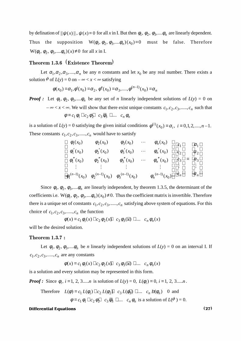
Theorem 1.3.6 (Existence Theorem)
Let 1 2 3, , ,...., nα α α α be any n constants and let x0 be any real number. There exists a
solution f of L(y) = 0 on – ¥ < x < ¥ satisfying
( –1)0 1 0 2 0 3 0( ) , ( ) , ( ) ,...., ( )φ α φ α φ α φ α′ ′′= = = =n
nx x x x
Proof : Let 1 2 3, , ,.... nφ φ φ φ be any set of n linearly independent solutions of L(y) = 0 on
– ¥ < x < ¥. We will show that there exist unique constants 1 2 3, , ,....., nc c c c such that
1 1 2 2 3 3 .... n nc c c cφ φ φ φ φ= + + + +
is a solution of L(y) = 0 satisfying the given initial conditions ( )0( ) , 0,1,2,...., –1.φ α= =i
ix i n
These constants 1 2 3, , ,....., nc c c c would have to sartisfy
1 0 2 0 3 0 01 1
1 0 2 0 3 0 0 2 2
3 31 0 2 0 3 0 0
( –1) ( –1) ( –1) ( –1)1 0 2 0 3 0 0
( ) ( ) ( ) ( )
( ) ( ) ( ) ( )
( ) ( ) ( ) ( )
( ) ( ) ( ) ( )
′ ′ ′ ′ =′′ ′′ ′′ ′′
L
L
L
M MM M M M
n
n
n
n n n n n nn
x x x x cx x x x c
cx x x x
cx x x x
φ φ φ φ αφ φ φ φ α
αφ φ φ φ
αφ φ φ φ
Since 1 2 3, , ,.... nφ φ φ φ are linearly independent, by theorem 1.3.5, the determinant of the
coefficients i.e. 1 2 3 0W( , , ,.... ) ( ) 0.n xφ φ φ φ ≠ Thus the coefficient matrix is invertible. Therefore
there is a unique set of constants 1 2 3, , ,....., nc c c c satisfying above system of equations. For this
choice of 1 2 3, , ,....., nc c c c the function
1 1 2 2 3 3( ) ( ) ( ) ( ) .... ( )n nx c x c x c x c xφ φ φ φ φ= + + + +
will be the desired solution.
Theorem 1.3.7 :
Let 1 2 3, , ,.... nφ φ φ φ be n linearly independent solutions of L(y) = 0 on an interval I. If
1 2 3, , ,....., nc c c c are any constants
1 1 2 2 3 3( ) ( ) ( ) ( ) .... ( )n nx c x c x c x c xφ φ φ φ φ= + + + +
is a solution and every solution may be represented in this form.
Proof : Since , 1, 2, 3.....i i nφ = is solution of L(y) = 0, ( ) 0, 1, 2, 3.....iL i nφ = = .
Therefore 1 1 2 2 3 3( ) ( ) ( ) ( ) .... ( ) 0n nL c L c L c L c Lφ φ φ φ φ= + + + + = and
1 1 2 2 3 3 .... n nc c c cφ φ φ φ φ= + + + + is a solution of L(f ) = 0.
(27)

Differential Equations
Let f be any solution of L(y) = 0 and x0 be in I.
Suppose ( –1)0 1 0 2 0 3 0( ) , ( ) , ( ) ,...., ( ) .φ α φ α φ α φ α′ ′′= = = =n
nx x x x
By existence theorem 1.3.6 there exist unique constants 1 2 3, , ,....., nc c c c such that
1 1 2 2 3 3 .... n nc c c cψ φ φ φ φ= + + + +is a solution of L(y) = 0 on I satisfying
( –1)0 1 0 2 0 3 0( ) , ( ) , ( ) ,...., ( )ψ α ψ α ψ α ψ α′ ′′= = = =n
nx x x x
The uniqueness theorem 1.3.4 implies that f = y. Thus 1 1 2 2 3 3 .... .n nc c c cφ φ φ φ φ= + + + +
Theorem 1.3.8Let 1 2 3, , ,.... nφ φ φ φ be n solutions of L(y) = 0 on an interval I constaining a point x0. Then
1 0– ( – )1 2 3 1 2 3 0W( , , ,.... ) ( ) W( , , ,.... ) ( )= a x x
n nx e xφ φ φ φ φ φ φ φProof :
1 2 3
1 2 3
1 2 3 1 2 3
( –1) ( –1) ( –1) ( –1)1 2 3
( ) ( ) ( ) ( )
( ) ( ) ( ) ( )
W( , , ,...., ) ( ) ( ) ( ) ( ) ( )
( ) ( ) ( ) ( )
′ ′ ′ ′
= ′′ ′′ ′′ ′′
L
L
L
M M M M
n
n
n n
n n n nn
x x x x
x x x x
x x x x x
x x x x
φ φ φ φ
φ φ φ φφ φ φ φ φ φ φ φ
φ φ φ φBy differentiating above determinant row-wise we get,
1 2 3
1 2 3
1 2 3 1 2 3
( –1) ( –1) ( –1) ( –1)1 2 3
W ( , , ,...., ) ( )
φ φ φ φ
φ φ φ φφ φ φ φ φ φ φ φ
φ φ φ φ
′ ′ ′ ′
′ ′ ′ ′′ = ′′ ′′ ′′ ′′
L
L
L
M M M M
n
n
nn
n n n nn
x
1 2 3 1 2 3
1 2 3 1 2 3
1 2 3 1 2 3
( –1) ( –1) ( –1) ( –1) ( ) ( ) ( ) ( )1 2 3 1 2 3
....
φ φ φ φ φ φ φ φ
φ φ φ φ φ φ φ φ
φ φ φ φ φ φ φ φ
φ φ φ φ φ φ φ φ
′′ ′′ ′′ ′′ ′ ′ ′ ′
+ + +′′ ′′ ′′ ′′ ′′ ′′ ′′ ′′
L L
L L
L L
M M M M M M M M
L L
n n
n n
n n
n n n n n n n nn n
Since two rows are identical the value of first (n – 1) determinants is zero. Therefore
1 2 3
1 2 3
1 2 3 1 2 3
( ) ( ) ( ) ( )1 2 3
W ( , , ,...., ) ( )
φ φ φ φ
φ φ φ φφ φ φ φ φ φ φ φ
φ φ φ φ
′ ′ ′ ′
′ = ′′ ′′ ′′ ′′
L
L
L
M M M M
n
n
n n
n n n nn
x
(28)

Differential Equations
Since each , 1,2,3,....,i i nφ = is a solution of L(y) = 0 ( ) ( –1) ( –2)1 2– (n n n
i i ia aφ φ φ= +
( –3)3 .... ).n
i n ia aφ φ+ + Hence,
1 2 3
1 2 3
1 2 3( –2) ( –2) ( –2) ( –2)
1 2 3( –1) ( –1) ( –1) ( –1)
1 1 1 2 1 3 1
( ) ( ) ( ) ( )
( ) ( ) ( ) ( )
W ( , , ,..., ) ( )
( ) ( ) ( ) ( )
– ( ) – ( ) – ( ) – ( )
φ φ φ φ
φ φ φ φφ φ φ φ
φ φ φ φ
φ φ φ φ
′ ′ ′ ′
′ =
L
L
M M M L M
L
n
n
nn n n n
nn n n n
n
x x x x
x x x x
x
x x x x
a x a x a x a x
Since,1 2 3
1 2 3
( –2) ( –2) ( –2) ( –2)1 2 3
( – ) ( – ) ( – ) ( – )1 2 3
( ) ( ) ( ) ( )
( ) ( ) ( ) ( )
0
( ) ( ) ( ) ( )
– ( ) – ( ) – ( ) – ( )
φ φ φ φ
φ φ φ φ
φ φ φ φ
φ φ φ φ
′ ′ ′ ′
=
L
L
M M M L M
L
n
n
n n n nn
n k n k n k n kk k k k n
x x x x
x x x x
x x x x
a x a x a x a x
for k = 2, 3, 4,....n, as two rows of the determinant are constant multiplies of each other are
Thus,
1 2 3
1 2 3
1 2 3 1 1 2 3
( –1) ( –1) ( –1) ( –1)1 2 3
( ) ( ) ( ) ( )
( ) ( ) ( ) ( )
W ( , , ,..., ) ( ) – ( ) ( ) ( ) ( )
( ) ( ) ( ) ( )
φ φ φ φ
φ φ φ φφ φ φ φ φ φ φ φ
φ φ φ φ
′ ′ ′ ′
′ = ′′ ′′ ′′ ′′
L
L
L
M M M M
L
n
n
n n
n n n nn
x x x x
x x x x
x a x x x x
x x x x
1 1 2 3– W( , , ,..., ) ( )na xφ φ φ φ=
Thus 1W Wa′ + = 0. On integrating this equation between the limits x0 to x we get ,
1 010W( ) W ( )= a xa xe x e x
or 1 0– ( – )0W( ) W( )a x xx e x=
Thus 1 0– ( – )1 2 3 1 2 3 0W( , , ,..., ) ( ) W( , , ,..., ) ( )a x x
n nx e xφ φ φ φ φ φ φ φ=
Theorem 1.3.9
Let 1 2 3, , ,.... nφ φ φ φ be n solutions of L(y) = 0 on an interval I containing x0. Then they are
linearly independent on I if and only if 1 2 3 0W( , , ,..., ) ( ) 0n xφ φ φ φ ≠
(29)

Differential Equations
Proof : By theorem 1.3.5 the solutions 1 2 3, , ,.... nφ φ φ φ of L(y) = 0 are linearly independent
on an interval I if and only if 1 2 3W( , , ,..., ) ( ) 0φ φ φ φ ≠n x for all x in I.
But 1 0– ( – )1 2 3 1 2 3 0W( , , ,..., ) ( ) W( , , ,..., ) ( )a x x
n nx e xφ φ φ φ φ φ φ φ= (by theorem 1.3.8.)
Therefore 1 2 3W( , , ,..., ) ( ) 0n xφ φ φ φ ≠ if and only if 1 2 3 0W( , , ,..., ) ( ) 0n xφ φ φ φ ≠ and the result
follows.
EXAMPLES
Q.1. Consider the equation
(5) (4)– – 0y y y y′ + =(a) Compute five linearly independent solutions.
(b)Compute the wronkian of the solutions found in (a).
(c) Find that solution f satisfying(4)(0) 1, (0) (0) (0) (0) 0.φ φ φ φ φ′ ′′ ′′′= = = = =
Ans (a) :
The characteristic equation
5 4( ) – – 1= +p r r r r
4( –1) – ( –1)= r r r
4( –1) ( –1)r r=
2 2( –1)( 1) ( –1)r r r= +
2( 1)( –1) ( 1)( –1)r r r r= + +Thus the characteristic roots are 1, 1, –1, i, – i
Therefore –1 2 3 4( ) , ( ) , ( ) , ( ) sinx x xx e x xe x e x xφ φ φ φ= = = = 5( ) cosφ =x x are solutions
of the given differential equation.
Ans (b) :0– ( – )
1 2 3 4 5 1 2 3 4 5 0W( , , , , ) ( ) W( , , , , ) ( )a x xx e xφ φ φ φ φ φ φ φ φ φ=
For the given equation a1 = – 1. Let x0 = 0 then
1 2 3 4 5 1 2 3 4 5W( , , , , ) ( ) W( , , , , ) (0).xx eφ φ φ φ φ φ φ φ φ φ=–
–
–1 2 3 4 5
–
–
sin cos
(1 ) – cos – sin
W( , , , , ) ( ) (2 ) – sin – cos
(3 ) – – cos sin
(4 ) sin cos
+= +
+
+
x x x
x x x
x x x
x x x
x x x
e xe e x x
e x e e x x
x e x e e x x
e x e e x x
e x e e x x
φ φ φ φ φ
(30)

Differential Equations
1 2 3 4 5
1 0 1 0 1
1 1 –1 1 0
W ( , , , , ) (0) 1 2 1 0 –1
1 3 –1 –1 0
1 4 1 0 1
=φ φ φ φ φ
The row transformations
2 1 3 1 4 1 5 1– , – , – , – givesR R R R R R R R
1 2 3 4 5
1 0 1 0 1
0 1 –2 1 –1
W( , , , , ) (0) 0 2 0 0 –2
0 3 –2 –1 –1
0 4 0 0 0
φ φ φ φ φ =
1 –2 1 –1
2 0 0 –2
3 –2 –1 –1
4 0 0 0
=
0 0 –2 2 0 –2 2 0 0
–2 –1 –1 2 3 –1 –1 3 –2 –1
0 0 0 4 0 0 4 0 0
= + +
2 0 0
3 –2 –1 – 32
4 0 0
+ =
Thus, 1 2 3 4 5 1 2 3 4 5W( , , , , ) W( , , , , ) (0) –32= =x xe eφ φ φ φ φ φ φ φ φ φ
Ans (c) :
The general solution f is –1 2 3 4 5( ) sin cosφ = + + + +x x xx c e c xe c e c x c x
The initial conditions (iv)(0) 1, (0) (0) (0) (0) 0φ φ φ φ φ′ ′′ ′′′= = = = = gives the followingsystem of equations.
1
2
3
4
5
1 0 1 0 1 1
1 1 –1 1 0 0
1 2 1 0 –1 0
1 3 –1 –1 0 0
1 4 1 0 1 0
+ =
c
c
c
c
c
The row transformation 2 1 3 1 4 1 5 1– , – , – , –R R R R R R R Rgives
(31)

Differential Equations
1
2
3
4
5
1 0 1 0 1 1
0 1 –2 1 –1 –1
0 2 0 0 –2 –1
0 3 –2 –1 –1 –1
0 4 0 0 0 –1
+ =
c
c
c
c
c
Solving the above system of equations simultaneously we get the values of c1, c2,c3, c4, c5.
From last equation we get 4c2 = – 1 gives 21
–4
c =
From the third row of the above system we get,
2 5 51
2 – 2 –1 gives4
c c c= =
From second and fourth row we get,
2 3 4 5– 2 – –1c c c c+ =
2 3 4 53 – 2 – – –1=c c c c
Substitution of c2 and c5 in above equations give
3 41
–2 –2
c c+ =
3 4–2 – 0=c c
Thus, 3 41 1
, –8 4
c c= =
From first row we get, 158
c =
Thus, –1 2 3 4 5( ) sin cosφ = + + + +x x xx c e c xe c e c x c x
–5 1 1 1 1
– – sin cos8 4 8 4 4
x x xe xe e x x= + +
is the required solution.
Q.2. Find all solutions of the following equations.
(a) – 8 0y y′′′ = (b) (4) 16 0+ =y y (c) – 5 6 0y y y′′′ ′′ ′+ =
(d) ( ) –16 0ivy y = (e) – 3 – 2 0y y y′′′ ′ = (f) (4) 5 4 0y y y′′+ + =
Ans. (a) :
The characteristic polynomial is 3( ) – 8p r r= and its roots are 2, –1 3 , –1– 3i i+
Thus, three linearly independent solutions are given by 2 (–1 3 ) (–1– 3 ), ,+x i x i xe e e and any
solution f has the form 2 (–1 3 ) (–1– 3 )1 2 3( )φ += + +x i x i xx c e c e c e where c1, c2, c3 are any
constants.
(32)

Differential Equations
Ans. (b) : The characteristic polynomial is 4( ) 16p r r= +
4 4 2 2 2 2( ) – (2 ) ( (2 ) ) ( – (2 ) )= = +p r r i r i r i
2 2 2 2 2( – (2 ) ) ( – ( 2) )r i i r i=
( 2 ) ( – 2 ) ( 2 ) ( – 2 )= + +r i i r i i r i r i
Thus, ( ) ( 2 ) ( – 2 ) ( 2 ) ( – 2 )= + +p r r i i r i i r i r i
2cos sin2 2
ππ π= + =
ii i e
\
1
22 4 cos sin
4 4
π ππ π
= = = +
i ii e e i
Therefore (1 )1 –1
,2 2 2
i ii ii i i
++ += = =
The roots of characteristic polynomial are – 2(–1 ), 2(–1 ), 2(1 ), – 2(1 )+ + + +i i i i
Thus four linearly independent solutions are
( 2 – 2) (– 2 2 ) ( 2 2), , ,i x i x i xe e e+ + (– 2 – 2)i xe
and every solution f has the form
( 2 – 2) (– 2 2) ( 2 2) (– 2 – 2)1 2 3 4( ) i x i x i x i xx c e c e c e c eφ + += + + +
Ans. (c) : The characteristic polynomial is 3 2( ) – 5 6p r r r r= + and its roots are 0, 3, 2. Thusthree linearly independent solutions are given by 1, e3x, e2x and any solution f has the
form 3 21 2 3( ) x xx c e c e cφ = + +
Ans. (d) : The characteristic polynomial is 4 2 2( ) –16 ( 4)( – 4) ( 2 )( – 2 )p r r r r r i r i= = + = +
( 2) ( – 2)r r+ and its roots are 2, – 2, 2i, –2i. Thus four linearly independent solutions are
given by 2 –2, , cos 2 , sin 2x xe e x x and every solution f has the form
2 –21 2 3 4( ) cos2 sin 2x xx c e c e c x c xφ = + + +
Ans. (e) : The characteristic polynomial is
3 2( ) – 3 – 2 ( 1) ) ( – – 2)= = +p r r r r r r
and its roots are 1 5 1– 5
–1, , .2 2
+
Thus, three linearly independent solutions are
1– 5(1 5) 2– 2, , ,
+
x xxe e e and every solution
f has the form1– 5
( )2
1 5( )– 2
1 2 3( )xxxx c e c e c eφ
+
= + +(33)

Differential Equations
Ans. (f) : The characteristic polynomial is
4 2 2 2( ) 5 4 ( 4) ( 1)p r r r r r= + + = + +and its roots are 2i , –2i , i , –i . Thus four linearly independent solutions are
cos2 , sin 2 , cos , sinx x x x and every solution f has the form
1 2 3 4( ) cos 2 , sin 2 cos sin .x c x c x c x c xφ = + + +
Q.3. Consider the equation – 4 0y y′′′ ′ =
(a) Compute three linearly independent solutions.
(b)Compute the wronkian of the solutions found in (a).
(c) Find the solution f satisfying
(0) 0, (0) 1, (0) 0φ φ φ′ ′′= = =
Ans. (a) : The characteristic polynomial 3( ) – 4p r r r= and its roots are 0, 2, –2. Thus, three
linearly independent solution are 2 –21, ,x xe e e° = and every solution f has the form
2 –21 2 3( ) x xx c c e c eφ = + +
Ans. (b) :
0( –0)1 2 3 1 2 3W( , , ) ( ) W( , , ) (0)xx eφ φ φ φ φ φ=
2 –2
2 –21 2 3
2 –2
1
W( , , ) ( ) 0 2 –2
0 4 4
x x
x x
x x
e e
x e e
e e
φ φ φ =
1 2 3
1 1 1
W( , , ) (0) 0 2 –2
0 4 4
φ φ φ =
Thus, 1 2 3W( , , ) ( ) 16xφ φ φ = .
Ans. (c) :
(0) 0, (0) 1, (0) 0,φ φ φ′ ′′= = =2 –2
1 2 3 1 2 3( ) , (0) 0x xx c c e c e c c cφ φ= + + = + + = and so on
1
2
3
1 1 1 0
0 2 –2 1
0 4 4 0
c
c
c
=
R3 – 2 R2 gives
1
2
3
1 1 1 0
0 2 –2 1
0 0 8 –2
c
c
c
=
(34)

Differential Equations
Therefore 3 2 3 2 3 21 1 1
– , 2 – 2 1 –4 2 4
= = ⇒ = ⇒ =c c c c c c
1 2 3 10 0c c c c+ + = ⇒ =
Thus, ( )2 –2 2 –21 2 3
1( ) –
4x x x xx c c e c e e eφ = + + = is the required solution.
EXERCISE
1. Are the following statements true or false ?
(a) If 1 2 3, , ,...., nφ φ φ φ are linearly independent functions on an interval I, then any subset of
them forms a linearly independent set of functions on I.
(b) If 1 2 3, , ,...., nφ φ φ φ are linearly dependent functions on an interval I, then any subset of
them forms a linearly dependent set of functions on I.
2. Are the following sets of functions defined on – ¥ < x < ¥ linearly independent ordependent ? why ?
(a) 21 2 3( ) 1, ( ) , ( )x x x x xφ φ φ= = =
(b) 1 2 3( ) , ( ) sin , ( ) 2cosi xx e x x x xφ φ φ= = =
(c) 21 2 3( ) , ( ) , ( ) | |xx x x e x xφ φ φ= = =
3. Find a basis of solutions of the differential equations.
(a) 5 4 0y y′′ ′+ + = (b) 6 12 8 0y y y y′′′ ′′ ′+ + + =
(c) (4) – 0y y =
4. Find the general solution of each of the following equations.
(i) 4
321 26 –11 4 0 (Ans. ( ) )′′ ′ + = = +
xx
y y y y x c e c e
(ii) (–1 2) (–1– 2)1 22 – 0 (Ans. ( ) )+′′ ′+ = = +x xy y y y x c e c e
(iii) 2 –31 2 3– 6 0 (Ans. ( ) )x xy y y y x c c e c e′′′ ′′ ′+ = = + +
(iv) (4) 2 – 21 2 3 4– 2 0 (Ans. ( ) )x xy y y x c c x c e c e′′ = = + + +
(v) ( )–2 2 21 2 38 0 Ans. ( )′′′ + = = + +x x xy y y x c e c e c xe
5. For each of the following equations find a particular solution which satisfies the giveninitial conditions.
(i) 0, (1) 2, (1) –1y y y′′ ′= = =(ii) 4 4 0, (0) 1, (0) 1y y y y y′′ ′ ′+ + = = =
(35)

Differential Equations
(iii) – 2 5 0, (0) 2, (0) 4y y y y y′′ ′ ′+ = = =
(iv) ( ) ( )2 2– 4 20 0, 0, 1′′ ′ ′+ = = =y y y y yπ π
(v) 3 5 – 0, (0) 0, (0) 1, (0) –1′′′ ′′ ′ ′ ′′+ + = = = =y y y y y y y
[Ans. : (i) ( ) 3 – ,y x x= (ii) –2( ) (1 3 ) xy x x e= + (iii) ( ) (2cos 2 sin 2 )xy x e x x= +
(iv) 2 –1
sin 44
xe xπ(v) –39 9
– .16 4 16
xxx
y e e = + ]
Ans. 1 :
(a) True (b) false
Ans. 2 :
(a) independent (b) dependent (iii) independent
Ans. 3 :
(a) –4 –1 2( ) , ( )x xx e x eφ φ= =
(b) –2 –2 2 –21 2 3( ) , ( ) , ( )x x xx e x xe x x eφ φ φ= = =
(c) –1 2 3 4( ) , ( ) , ( ) cos , ( ) sinx xx e x e x x x xφ φ φ φ= = = =
Unit 4 : The Non-Homogeneous Equation of Order nWe now return to the nth order non-homogeneous linear differential equation with constant
coefficients. In the first part we will discuss the method of finding all solutions of the secondorder non-homogeneous equation.
1 2( ) ( ),L y y a y a y b x′′ ′= + + =
Where b is some continuous function on an interval I. The general solution of the aboveequation is
( ) ( ) ( ),c py x y x y x= +
where, yc(x), the complementary function is the general solution of the related homogenousequation and yp(x) is a particular solution of the equation.
Suppose we know that yp is a particular solution of the equation L(y) = b(x) and let y beany other solution. Then,
( – ) ( ) – ( ) ( ) – ( ) 0p pL L L b x b xψ ψ ψ ψ= = =
on I. This shows that y –yp is a solution of the homogenous equation L(y) = 0. Therefore if f 1,f 2 are linearly independent solutions of L(y) = 0, there are unique constants c1, c2 such that
(36)

Differential Equations
1 1 2 2– p c cψ ψ φ φ= +In other words every solution y of L(y) = b (x) can be written in the form
1 1 2 2p c cψ ψ φ φ= + +
The problem of finding all solutions of L(y) = b (x) reduces to finding a particularsolution yp.
Theorem 1.4.1Let b(x) be continuous on an interval I. Every solution y of L(y) = b (x) on I can be
written as 1 1 2 2p c cψ ψ φ φ= + + .
Where yp is a particular solution, f1, f2 are two linearly independent solutions of L(y) = 0and c1, c2 are constants. A particular solution yp is given by
0
1 2 1 2
1 2
[ ( ) ( ) – ( ) ( )] ( )( ) .
W( , ) ( )
x
px
t x x t b tx dt
t
φ φ φ φψφ φ
= ∫
Conversely every such y is a solutions of L(y) = b (x)
Proof :
Let y and yp be two solutions of
1 2( )L y y a y a y b′′ ′= + + =
Then ( – ) ( ) – ( ) 0p pL L Lψ ψ ψ ψ= =
This shows that – pψ ψ is a solution of a homogeneous equation L(y) = 0. By theorem
1.1.1 there exist two linearly independent solutions f1, f2 and every solution of L(y) = 0 is of the
form 1 1 2 2c cφ φ+ where c1 and c2 are constants. Such a function 1 1 2 2c cφ φ+ cannot be a solution
of L(y) = b(x) unless b(x) = 0 on I.
Suppose 1 1 2 2( ) ( ) ( ) ( ) ( )x u x x u x xφ φ φ= + is a solution of L(y) = b(x) on I.
(This procedure is called as the variation of constants.)
Then
1 1 2 2 1 1 1 2 2 2 1 1 2 2( ) ( ) ( ) ( )u u a u u a u u b xφ φ φ φ φ φ′′ ′+ + + + + =
i.e. 2 1 1 2 2 1 1 1 1 1 2 2 2 2( ) ( )a u u a u u u uφ φ φ φ φ φ′ ′ ′ ′+ + + + +
1 1 1 1 1 1 2 2 1 1 2 2( 2 2 ) ( )u u u u u u b xφ φ φ φ φ φ′′ ′ ′ ′′ ′′ ′ ′ ′′+ + + + + + =
Therefore
1 1 1 1 2 1 2 2 1 2 2 2( ) ( )u a a u a aφ φ φ φ φ φ′′ ′ ′′ ′+ + + + +
1 1 1 2 1 1 2 2 1 1 1 2 2( ) 2( ) ( ) ( )u u u u a u u b xφ φ φ φ φ φ′′ ′′ ′ ′ ′ ′ ′ ′+ + + + + + =
i.e. 1 1 2 2 1 1 2 2 1 1 1 2 2( ) 2( ) ( ) ( )u u u u a u u b xφ φ φ φ φ φ′′ ′′ ′ ′ ′ ′ ′ ′+ + + + + =
(37)

Differential Equations
Observe that if
1 1 2 2u uφ φ′ ′+ = 0
then 1 1 2 2 1 1 2 2 1 1 2 2( ) ( ) ( )′ ′ ′ ′ ′ ′ ′′ ′′′+ = + + +u u u u u uφ φ φ φ φ φ
and 1 1 2 2 ( )u u b xφ φ′ ′ ′ ′+ =Thus if we can find two functions u1(x) and u2(x) such that
1 1 2 2 0u uφ φ′ ′+ =
1 1 2 2 ( )u u b xφ φ′ ′ ′ ′+ =
Then 1 1 2 2u uφ φ+ will satisfy L(y) = b(x).
On solving above two equations for 1u ′ and 2u ′we get,
2 11 2
1 2 1 2
–( ) , ( ) ,
W( , ) W( , )
φ φφ φ φ φ
′ ′= =b bu x u x
Integration of above equation between the limits x0 to x provides
0
21 1 0
1 2
( ) ( )( ) – ( )
W( , ) ( )
x
x
t b tu x dt u x
t
φφ φ
= +∫
and0
12 2 0
1 2
( ) ( )( ) ( ).
W( , ) ( )
x
x
t b tu x dt u x
t
φφ φ
= +∫
The solution 1 1 2 2u uφ φ+ takes the form
0
21 1 0
1 2
( ) ( )( ) ( ) – ( )
W( , ) ( )
x
x
t b tx x dt u x
t
φφ φφ φ
= +
∫
0
12 2 0
1 2
( ) ( )( ) ( )
W( , ) ( )
φφφ φ
+ + +
∫x
x
t b tx dt u x
t
The term 1 1 0 2 2 0( ) ( ) ( ) ( )x u x x u xφ φ+ is a complementary function or the solution of
corresponding homogeneous equation L(y) = 0 and the particular solution takes the form
0 0
2 11 2
1 2 1 2
( ) ( ) ( ) ( )( ) – ( ) ( )
W( , ) ( ) W( , ) ( )
x x
px x
t b t t b tx x dt x dt
t t
φ φψ φ φφ φ φ φ
= +∫ ∫
0
1 2 2 1
1 2
[ ( ) ( ) – ( ) ( )] ( )( )
W( , ) ( )
x
px
t x t x b tx dt
t
φ φ φ φψφ φ
= ∫
The function yp(x) is a solution of L(y) = b (x).
Theorem 1.4.1 provides a method to find a solution of second order non-homogeneousdifferential equation with constant coefficients. The same procedure can be generalized for thenon-homogeneous equation of order n.
(38)

Differential Equations
Theorem 1.4.2
Let b be continuous on an interval I and let 1 2 3, , ,...., nφ φ φ φ be n linearly independent
solutions of ( ) ( –1) ( –2)1 2( ) .... 0n n n
nL y y a y a y a y= + + + + = on I. Every solution y of L(y) =
b(x) can be written as
1 1 2 2 3 3 ....ψ ψ φ φ φ φ= + + + + +p n nc c c c
Where yp is a particular solution of L(y) = b(x) and 1 2 3, , ,......, nc c c c are constants. Everysuch y is a solution of L(y) = b(x). A particular solution yp is given by
01 1 2 3
( ) ( )( ) ( ) .
W( , , ,...., ) ( )
xnk
p kk nx
W t b tx x dt
tψ φ
φ φ φ φ== ∑ ∫
Proof : The proof is similar to the proof of theorem 1.4.1 Let b be continuous function on aninterval I. Consider the differential equation
( ) ( –1) ( –2)1 2( ) .... ( )n n n
nL y y a y a y a y b x= + + + + =
where, a1, a2, a3,..., an are constants. If yp is a particular solution of L(y) = b(x) and y is anyother solution of L(y) = b(x), then
( – ) ( ) – ( ) ( ) – ( ) 0ψ ψ ψ ψ= = =p pL L L b x b x
and y – yp is a solution of corresponding homogeneous equation L(y) = 0. (is called subtractionprinciple).
Thus any solution y of L(y) = b(x) can be written in the form
1 1 2 2 3 3 ....p n nc c c cψ ψ φ φ φ φ= + + + + +
where, yp is a particular solution of L(y) = b(x), the functions 1 2 3, , ,...., nφ φ φ φ are n linearly
independent solutions of L(y) = 0 (determined in theorem 1.3.1) and 1 2 3, , ,..., nc c c c are constants.
To find a particular solution yp we use the variation of constants method. Suppose
1 1 2 2 3 3( ) ( ) ( ) ( ) ( ) ( ) .... ( ) ( )p n nu x x u x x u x x u x xψ φ φ φ φ= + + + +
is a solution of L(y) = b(x). Since yp is a solution it satisfies the equation i.e L(yp) = b(x).
1 1 2 2 3 3 ....p n nu u u uψ φ φ φ φ= + + + +
1=
= ∑n
i ii
u φ
Then, 1 1 1 1 2 2 2 2 ....ψ φ φ φ φ φ φ′ ′ ′ ′ ′ ′ ′= + + + + + +p n n n nu u u u u u
1 1 2 2 3 3 1 1 2 2( .... ) ( .... )n n n nu u u u u u uφ φ φ φ φ φ φ′ ′ ′ ′ ′ ′ ′= + + + + + + + +
1 1
φ φ= =
′ ′= +∑ ∑n n
i i i ii i
u u
Let 0i iu φ′∑ = then ψ φ′ ′= ∑p i iu
We have ψ φ φ′′ ′′ ′ ′= ∑ + ∑p i i i iu u
(39)

Differential Equations
Suppose 0i iu φ′ ′∑ = then p i iuψ φ′′ ′′= ∑
Continuing the same assumptions we get,
( –2) ( –1) ( –1)
0 ;
0 ;
0 ;
0 ;
i i p i i
i i p i i
i i p i i
n n ni i p i i
u u
u u
u u
u u
φ ψ φ
φ ψ φ
φ ψ φ
φ ψ φ
′ ′ ′∑ = = ∑
′ ′ ′′ ′′∑ = = ∑
′ ′′ ′′′ ′′′∑ = = ∑
′∑ = = ∑
M
( ) ( –1) ( )n n np i i i iu uψ φ φ′= ∑ + ∑
If ( –1) ( )ni iu b xφ′∑ = then ( ) ( ) ( )n n
p i iu b xψ φ= ∑ + and ( )pL ψ becomes
( ) ( –1) ( –2)1 2( ) ( ) .... .ψ φ φ φ φ = ∑ + + ∑ + ∑ + + ∑
n n np i i i i i i n i iL u b x a u a u a u
( ) ( –1)
1( ) .....φ φ φ = + ∑ + + + n n
i i i n ib x u a a
Thus, ( ) ( )pL b xψ = and therefore yp is a solution of L(y) = b (x). Therefore the problem
is now reduced to solving the system given below for the functions u1, u2, u3,..., un.
( –2)
( –1)
0
0
0
0
( )
φ
φ
φ
φ
φ
′∑ =
′ ′∑ =
′ ′′∑ =
′∑ =
′∑ =
M
i i
i i
i i
ni i
ni i
u
u
u
u
u b x
Thus, we have system of equations
1 2 31
1 2 3 2
31 2 3
( –1) ( –1) ( –1) ( –1)1 2 3
0
0
0
( )
n
n
n
n n n n nn
u
u
u
u b x
φ φ φ φ
φ φ φ φ
φ φ φ φ
φ φ φ φ
′ ′ ′ ′ ′ ′ ′ =′′ ′′ ′′ ′′ ′
L
L
L
M MM
L
By solving above system of equations by Cramer’s rule we get,
1 2 3
W ( ) ( )( ) , 1,2,3,.....,
( , , ,...., ) ( )k
kn
x b xu x k n
W xφ φ φ φ′ = =
Where kW ( )x is the determinant obtained from 1 2 3W[ , , ,...., ]( )n xφ φ φ φ by replacing the
kth column i.e. ( –1)[ ..... ]n Tk k k kφ φ φ φ′ ′′ by [0 0 0....0 1] .T
If x0 is any point in I, we can integrate u¢k and the functions uk can be written as
(40)

Differential Equations
0 1 2 3
W ( ) ( )( ) 1,2,3,...., .
W( , , ,...., ) ( )
xk
knx
t b t dtu x k n
tφ φ φ φ= =∫
The particular solution yp now takes the form
0 1 2 3
W ( ) ( )( ) ( )
W( , , ,...., ) ( )ψ φ
φ φ φ φ= ∑ ∫
xk
p knx
t b t dtx x
t
Now we are in a position to find out a solution of the non-homogenous equation oforder n.
Observe that a particular solution yp satisfies
( –1)0 0 0 0( ) ( ) ( ) ...... ( ) 0.n
p p p px x x xψ ψ ψ ψ′ ′′= = = = =
EXAMPLES
Q.1. Compute the solution y of 1y y y y′′′ ′′ ′+ + + = which satisfies (0) 0, (0) 1,ψ ψ ′= =
(0) 0ψ ′′ = .
Ans. : The characteristic polynomial of the corresponding homogeneous equation is3 2( ) 1.p r r r r= + + + The characteristic roots are i, –i, 1. The basic solutions of the
corresponding homogeneous equation are
–1 2 3( ) cos ( ) sin ( ) xx x x x x eφ φ φ= = =
To obtain the particular solution of the form
1 1 2 2 3 3p u u uψ φ φ φ= + +We have to find W (f1, f2 , f3 ) (x) and Wk (t) for k = 1, 2, 3.
–
–1 2 3
–
cos sin
W( , , ) ( ) – sin cos –
– cos – sin
x
x
x
x x e
x x x e
x x e
φ φ φ =
1 0– ( – )1 2 3 1 2 3 0W( , , ) ( ) W( , , ) ( )= a x xx e xφ φ φ φ φ φ
–1 2 3W( , , ) (0)xe φ φ φ=
1 2 3
1 0 1
W( , , ) (0) 0 1 –1
–1 0 1
φ φ φ =
= 1[1 – 0] + 1 [0 + 1] = 2
Thus –1 2 3W( , , ) ( ) 2 xx eφ φ φ =
(41)

Differential Equations
–
– 3 1 – – –1
–
0 sin
W ( ) 0 cos – (–1) [– cos – sin ] – (cos sin )
–1 – sin
+= = = +
x
x x x x
x
x e
x x e e x e x e x x
x e
–
– –2
–
cos 0
W ( ) – sin 0 – (cos – sin )
– cos 1
= =
x
x x
x
x e
x x e e x x
x e
3
cos sin 0
W ( ) – sin cos 0 1
– cos – sin 1
x x
x x x
x x
= =
–
11 –
1 2 3
W ( ) ( ) (cos sin )( ) –
W( , , ) ( ) 2
+= =∫ ∫x x t
t
t b t e t tu x dt dt
t eφ φ φ
1
– [ sin – cos ]2
x x= +
Thus, 11
( ) [cos – sin ]2
u x x x=
–
22 –
1 2 3
W ( ) ( ) (cos – sin )( )
W( , , ) ( ) 2φ φ φ= =∫ ∫
x x t
t
t b t e t tu x dt dt
t e
1
[ sin cos ]2
x x= + +
3
3 –1 2 3
W ( ) ( ) 1( )
W( , , )( ) 22
x xx
t
t b t dt dtu x e
t eφ φ φ= = =∫ ∫
Therefore a particular solution is given by
1 1 2 2 3 3( ) ( ) ( ) ( ) ( ) ( )p u x x u x x u x xψ φ φ φ= + +
–1 1 1
– (cos – sin )cos (cos sin )sin 12 2 2
= + + + =x xx x x x x x e e
The most general solution is
1 1 2 2 3 3( ) px c c cψ ψ φ φ φ= + + +
–1 2 31 cos sin xc x c x c e= + + +
1 3(0) 0 1 0c cψ = ⇒ + + =
–1 2 3(0) 1 ( ) – sin cos – xx c x c x c eψ ψ′ ′= ⇒ = +
Thus, y¢ (0) = c2 – c3 = 1
–1 2 3( ) – cos – sin′′ = + xx c x c x c eψ
(42)

Differential Equations
1 3(0) – 0c cψ ′′ = + =
Solving the system of equations
1 + c1 + c3 = 0
c2 – c3 = 1
– c1 + c3 = 0
We get, 1 2 31 1 1
– , , –2 2 2
c c c= = =
Therefore the solution of our problem is given by
–1
( ) 1 (sin – cos – )2
xx x x eψ = +
Q.2. Find all solutions y of the following equations
(a) –y y x′′′ ′ =
(b) –– 3 2 sin xy y y e′′ ′ + =
(c) –24 4 3 xy y y xe′′ ′+ + =
Ans. (a) : The characteristic polynimial 3( ) –p r r r= has roots 0, 1, –1 and the linearly
independent solution of the related homogeneous equation are 1 2( ) 1, ( ) ,xx x eφ φ= =–
3( ) xx eφ =
Let 1 1 2 2 3 3( ) ( ) ( ) ( ) ( ) ( )p u x x u x x u x xψ φ φ φ= + +
1 2 3
W ( ) ( )( ) 1,2,3.
W( , , ) ( )φ φ φ= =∫
xk
kt b t ds
u x kt
–
–1 2 3
–
1
W( , , ) ( ) 0 – 2
0
φ φ φ = =
x x
x x
x x
e e
x e e
e e
–
–1
–
0
( )W ( ) 0 – –2= =
x x
x x
x x
e e
b x x e e x
x e e
–
–2
–
1 0
( )W ( ) 0 0 –
0
x
x x
x
e
b x x e xe
x e
= =
3
1 0
( )W ( ) 0 0
0
x
x x
x
e
b x x e xe
e x
= =
(43)

Differential Equations
2
1–2
( ) –2 2
= =∫x t dt x
u x
–– –
21 1
( ) – (1 )2 2 2
= = = +∫ ∫x xt
t xteu x dt t e dt x e
31 1
( ) ( –1)2 2 2
= = =∫ ∫x xt
t xte dtu x t e dt x e
2 2
1 1 2 2 3 31 1
– – (1 ) ( –1) – –12 2 2 2
= + + = + + =px x
u u u x xψ φ φ φ is the
required particular integral and the solution –1 2 3= + + +x x
pc c e c eψ ψ .
(b) : The characteristic polynomial 2( ) – 3 2p r r r= + has roots +2, +1 and therefore the two
linearly independent solution of the corresponding homogeneous equation are2
1 2( ) and ( )x xx e x eφ φ= =
Let 1 1 2 2( ) ( ) ( ) ( )p u x x u x xψ φ φ= + be a particular integral of the given differential equation
then by method of separation of parameters we get,
1 21 2
1 2 1 2
W ( ) ( ) W ( ) ( )( ) and ( )
W( , ) ( ) W( , ) ( )
x b x dx x b x dxu x u x
x xφ φ φ φ= =∫ ∫
where,2
31 1 2 2
W ( , ) ( ) ,2
= =x x
xx x
e ex e
e eφ φ
22 –
1 – 2
0( )W ( ) – sin ,
sin 2= =
xx x
x x
eb x x e e
e e
–2 –
0( )W ( ) sin .
sin
xx x
x x
eb x x e e
e e= =
Thus, – – –1( ) – sin – cosx x xu x e e dx e= =∫
and –2 – – – –
2( ) sin – sin cos= + = +∫ x x x x xu x e e dx e e e
[ Integrate above equation with the substitution t = e–x].
Then the general solution
1 1 2 2= + + pc cψ φ φ ψ
2 – – – – 21 2 (– cos ) (– sin cos )x x x x x x x xc e c e e e e e e e= + + + +
2 2 –1 2 – sin .x x x xc e c e e e= +
(c) : The characteristic polynomial 2( ) 4 4p r r r= + + has roots –2, –2 and therefore the twolinearly independent solution of the corresponding homogeneous equation are
–2 –21 2( ) , ( )x xx e x xeφ φ= =
(44)

Differential Equations
Let 1 1 2 2( ) ( ) ( ) ( )p u x x u x xψ φ φ= + be a particular integral of the given differential equation
then by method of separation of parameters we get,
1 21 2
1 2 1 2
W ( ) ( ) W ( ) ( )( ) , ( )
W( , )( ) W( , ) ( )
x b x dx x b x dxu x u x
x xφ φ φ φ= =∫ ∫
where, –2 –2
–2 –41 1 2 –2 –2
( ) 3 , W ( , ) ( ) ,–2 (1– 2 )
φ φ= = =x x
x xx x
e xeb x xe x e
e x e
–22 –4
1 –2 –2
0( )W ( ) –3 ,
3 (1– 2 )= =
xx
x x
xeb x x x e
xe x e
2–4
2 –2 –2
– 0( )W ( ) 3 .
–2 3= =
xx
x x
eb x x xe
e xe
Thus, 2 –4
31 –4
3( ) – – and
x
xx e
u x dx xe
= =∫
–4
22 –4
3 3( )
2= + =∫
x
x
xeu x dx x
e
Therefore3 –2 3 –2
1 1 2 23
–2
x xp u u x e x eψ φ φ= + = +
3 –21
2xx e=
The general solution
–2 –2 3 –2
1 212
= + +x x xc e c xe x eψ
Q.3. Find the general solution of
tan , – .2 2π π′′ + = < <y y x x
Ans : The characteristic polynimial 2( ) 1p r r= + has roots +i, –i and the two linearly independent
solutions are
1 2( ) cos and ( ) sinφ φ= =x x x x
Let 1 1 2 2( ) ( ) ( ) ( ) ( )p x u x x u x xψ φ φ= + be a particular integral of the given differential equation
then by method of separation of parameters we get,
1 21 2
1 2 1 2
W ( ) ( ) W ( ) ( )( ) , ( )
W( , ) ( ) W( , ) ( )
x b x dx x b x dxu x u x
x xφ φ φ φ= =∫ ∫
where, b(x) = tan x
(45)

Differential Equations
2
1 2 1cos sin 0 sin sin
W( , ) ( ) 1, ( )W ( ) – ,– sin cos tan cos cos
x x x xx b x x
x x x x xφ φ = = = =
2cos 0
( )W ( ) sin .– sin tan
= =x
b x x xx x
Therefore 2
1sin
( ) – – log (sec tan ) sincos
xu x dx x x x
x= = + +∫
2( ) sin – cosu x x d x x= =∫
and 2– cos log (sec tan ), –2
= + < <p x x x x ππψ
The general solution
1 2 2 2( ) cos sin – cos log(sec tan ), –= + + < <y x c x c x x x x xπ π
Note. The formula for a particular a solution yp of L(y) = b(x) makes sense for somediscontinuous functions b (x). Then yp will be a solution of L(y) = b(x) at the continuitypoints of b .
Q 4. Find a particular solution of the equation.
( ),y y b x′′ + =Where, ( ) –1 (– 0) ,
1 (0 ) ,0 (1 1 ).
b x xx
x
= Π ≤ <= ≤ ≤ Π= > Π
Ans : Let us find out the particular solution of α′′ + =y y where a is a constant.
The characteristic polynomial is 2( ) 1p r r= + and has roots +i, –i. Therefore the basic
solutions (linearly independent solutions) are
1 2( ) cos , ( ) sinx x x xφ φ= =
Let 1 1 2 2( ) ( ) ( )p u x x u xψ φ φ= + be a particular solution of the equation α′′ + =y y . By
method of separation of parameters we get,
1 2
1 21 2 1 2
W ( ) ( ) W ( ) ( )( ) , ( )
W( , )( ) W( , ) ( )
x b x dx x b x dxu x u x
x xφ φ φ φ= =∫ ∫
where, 1 2cos sin
W( , ) ( ) 1– sin cos
x xx
x xφ φ = =
1 20 sin cos 0
W ( ) – sin , W ( ) cos1 cos – sin 1
x xx x x x
x x= = = =
Then, 11
1 2
W ( ) ( ) – sin( ) cos
W( , ) ( ) 1α α
φ φ= = =∫ ∫
x b x dx xu x dx x
x
(46)

Differential Equations
22
1 2
W ( ) ( ) cos( ) sin
W( , )( ) 1α α
φ φ= = =∫ ∫
x b x xu x dx dx x
x
The particular solution
1
2 21 2 2 cos sin= + = + =p u u x xψ φ φ α α α
Thus the general solution of α′′ + =y y is
1 2cos sinψ α= + +c x c x
The general solution on the real line becomes
1 2
3 4
5 6
7 8
( ) cos sin ; – –
cos sin –1 ; – 0
cos sin 1 ; 0
cos sin ;
= + ∞ < <= + ≤ <= + + ≤ ≤
= + < < ∞
x c x c x x
c x c x x
c x c x x
c x c x x
ψ ππ
ππ
The continuity of y at – , 0,=x π π gives 1 3 3 5 5 7– – –1, –1 1, – 1 –= = + + =c c c c c c
Since we have three equations in 4 unknown, the particular solution yp will not be unique
e.g. choose *3 1 1c c= + and c2 = c4 = c6 = c8 = c
Then *1 cos sin+c x c xis a complementary function or the solution of corresponding
homogenous equation 0y y′′ + = and particular equation will be determined as follows.
If *3 1 1= +c c then *
1 3 11 2c c c= + = +*
3 1 1c c= +* *
5 3 1 1– 2 1– 2 –1c c c c= = + =* *
7 5 1 1–1 –1–1 – 2c c c c= = =
Thus, the particular solution becomes
( ) 2cos –= ∞ < <x x xψ πcos –1 – 0– cos 1 0–2cos
= ≤ <= + ≤ ≤= < < ∞
x xx xx x
ππ
π
If we choose *3 1 2c c= + then *
1 3 1
*3 1
*5 3 1
*7 5 1
1 3,
2,
– 2 ,
–1 –1,
c c c
c c
c c c
c c c
= + = +
= +
= =
= =and the particular solution becomes
( ) 3cos ; – –2cos –1 ; – 01 ; 0– cos ; .
= ∞ < <= ≤ <= ≤ ≤= < < ∞
x x xx x
xx x
ψ ππ
ππ
(47)

Differential Equations
Thus, we can generate infinitely many particular solutions that are piecewise continuous.
Method of undetermined coefficients :
The method described sofar is called the method of variation of parameters. Although thismethod yields a solution of the non-homogeneous equation it sometimes require more laborthan necessary. We now explain a method which is often faster than a method of variation ofparameters. This method is useful to solve the non-homogeneous equation L (y) = b (x), whenb(x) is a solution of some homogeneous equation with constant coefficients. The procedure weare about to describe is called the method of undetermined coefficients.
For the given different equation L (y) = b (x), suppose b(x) is a solution of somehomogeneous equation M (y) = 0 with constant coefficients. Then M (b(x)) = 0. If y is a solutionof L (y) = b (x) and M (b) = 0 then
[ ]( ) ( ) 0.M L M bψ = =
Therefore y is a solution of the homogeneous equation M (L(y)) = 0 with constantcoefficients. If the order of differential operator Lis n and that of M is m then M(L(y)) = 0 is ahomogeneous differential equation of order m + n and therefore there are m + n linearlyindependent solutions of M (L(x)) = 0. Since b(x) is a particular solution of M (y) = 0 everylinear combination of these n + m linearly independent solution will not be a solution ofL (y) = b (x). Thus, to fine the solution of L (y) = b (x) we substitute the linear combination ofsolutions into L (y) = b (x) and determine the set of coefficients other than the coefficients of thesolutions corresponding to the homogeneous equation L (y) = 0.
We give an example to show the usefulness of this method. Suppose we consider2( ) – 3 2L y y y y x′′ ′= + =
Since 2( ) 0,x ′′′ = x2 is a solution of ( ) 0.M y y′′′= =Every solution y of L (y) = x2 is a solution of
2( ( )) ( – 3 2 ) ( ) 0.M L y M y y y M x′′′ ′= + = =But ( – 3 2 ) ( – 3 2 ) 0M y y y y y y′′′ ′ ′′′ ′ ′′′+ = + =
i.e. ( ) ( )– 3 2 0.v ivy y y′′′+ =
The characteristic polynomial of this equation is 5 4 3( ) – 3 2p r r y r= + (just the product
of characteristics polynomials of L and M ). The roots of p (r) are 0, 0, 0, 1, 2 and hence y must
have the form 2 20 1 2 3 4
x xc c x c x c e c eψ = + + + + observe that 23 4
x xc e c e+ is a solution
of L (y) = 0.
Since we are interested only in particular solution y p of 2( ) ,L y x= we can assume
20 1 2p c c x c xψ = + +
Since y p is a solution, it should satisfy the differential equation L (y) = x2.
[ ] [ ]20 1 2 1 2 2( ) – 3 2 2 – 3 2 2p p p pL c c x c x c c x cψ ψ ψ ψ′′ ′ = + = + + + +
2( )pL xψ = gives 2 22 1 2 0 1 22 (2 – 6 ) (2 – 3 2 )c x c c x c c c x+ + + =
(48)

Differential Equations
Since the above equation should hold for all values of x, on equating the coefficients ofequal powers of x we get ,
2 1 2 0 1 22 1, 2 – 6 0, 2 – 3 2 0.= = + =c c c c c c
By solving these equations simultaneously we get,
2 1 01 3 7
, , .2 2 4
c c c= = =
Therefore,27 3 1
4 2 2p x xψ = + +
21
(2 6 7)4
x x= + +
is a particular solution of 2( )L y x=
and 23 4
x xp c e c eψ ψ= + +
2 2
3 41
(2 6 7)4
x xx x c e c eψ = + + + + is a general solution of – 3y y′′ ′ +
22 .y x=This method is also called as annihilator method since to solve L (y) = b (x), we find the
operator M which annihilates b(x). i.e. M (b (x)) = 0.
Once M has been found the problem becomes algebraic in nature.
EXAMPLES
Exp. 1. Using the annihilator method find a particular solution of each of the followingequations.
(a) 4 cosy y x′′ + = (b) 2 –– 4 3 4x xy y e e′′ = +
(c) 2– – 2 cosy y y x x′′ ′ = +
Ans. (a) : cos x is a solution of 0y y′′ + = therefore
( )M y y y′′= +
( ) 4L y y y′′= + therefore [ ] [ ]( ( )) ( ) ( )M L y L y L y′′= +
[ ]( ) ( 4 ) 4′′ ′′ ′′= + + +M L y y y y y
( ) 5 4′′= + +ivy y y
Thus, [ ( )] 0M L y = implies ( ) 5 4 0.ivy y y′′+ + =
The characteristic polynomial of the above equation is
4 2 2 2( ) 5 4 ( 4) ( 1)p r r r r r= + + = + +The root of p(r) are i, –i, +2i, – 2i and hence the solutions y have the form
(49)

Differential Equations
1 2 3 4cos sin cos 2 sin 2= + + +c x c x c x c xψ
observe that 3 4cos2 sin 2c x c x+ is a solution of ( ) 4 0.L y y y′′= + = Since we are interested only
in particular solution yp of L (y) = cos x, we can assume
1 2( ) cos sinp x c x c xψ = +
Since yp is a solution it should satisfy the differential equation 4 cos .y y x′′ + =
1 2 1 24 – cos – sin 4( cos sin ) cosψ ψ′′ + = + + =p p c x c x c x c x x
On equation the coefficients of cosx and sin x we get
1 23 1, 3 0c c= = i.e. 1 21
and 03
c c= =
Thus, particular solution 1
cos3p xψ =
Ans. (b) : 2 –3 4x xe e+ is a solution of (D – 2) (D – 1) = 0 i.e. – – 2 0.y y y′′ ′ =
Thus, ( ) – – 2′′ ′=M y y y y. since ( ) – 4L y y y′′= , ( )( ( )) – 4ivM L y y y′′′=– 6 4 8y y y′′ ′+ + .
The differential equation
( ) – 4 – 6 4 8 0ivy y y y y′′′ ′′ ′+ + =
has a characteristic polynomial 4 3 2( ) – 4 – 6 4 8.p r r r r r= + + The roots of characteristic
polynomial are 2, 2, –1, –2.
The solution y has the form
2 2 – –21 2 3 4( ) x x x xx c e c xe c e c eψ = + + +
Observe that 2 –21 4+x xc e c e is a solution of the homogeneous equation L(y) = 0.
Since we are only interested in particular solution assume the solution
2 2 –1 2 3ψ = + +x x x
p c e c xe c e
Since yp is a particular solution is should satisfy the equation 2 –– 4 3 4′′ = +x xy y e e
[ ] 2 –1 2 32 (1 2 ) –′ = + + x x
p c x c e c eψ
[ ] 2 –1 2 34 (4 4 ) x x
p c x c e c eψ ′′ = + + +
[ ] 2 –1 2 1 2 3– 4 4 (4 4 ) – 4 – 4 – 3x x
p p c x c c xc e c eψ ψ′′ = + +
But yp satisfies 2 –– 4 3 4x xy y e e′′ = +
Therefore [ ] 2 – 2 –2 34 – 3 3 4x x x xc e c e e e= +
By comparing coefficient of e2x and e–x we get 4c2 = 3 and –3c3 = 4
(50)

Differential Equations
Thus, 2 2 – –21 4
3 4–
4 3x x x xc e xe e c eψ = + + and particular integral
2 –3 4– .
4 3x x
p xe eψ =
Ans. (c) : 2 cosx x+ is a solution of 3 2( 1) 0D D y+ = i.e. ( ) 0.vy y′′′+ = Thus ( )( ) vM y y y′′′= +( ) – – 2L y y y y′′ ′=
Therefore [ ] [ ] [ ]( )( ) – – 2 – – 2
vM L y y y y y y y′′′′′ ′ ′′ ′= +
(7) (6) (5) (4)– – – – 2 0.y y y y y′′′= =
The differential equation [ ]( ) 0M L y = has a characteristic polynomial 7 6( ) –p r r r=5 4 3– – – 2r r r .
The roots of characteristic polynomial are 1 5 1– 5
0, 0, 0, , – , and2 2
i i+
.
The solution y must have the form
1 5 1– 5
2 220 1 2 3 4 5 6( ) cos sinψ
+
= + + + + + +x x
x c c x c x c x c x c e c e
The expression
1 5 1– 5
2 2
5 6
+
+x x
c e c e is a solution of the homogeneous equation
( ) – – 2 0.L y y y y′′ ′= =Since we are interested in particular solution assume the solution
20 1 2 3 4cos sinp c c x c x c x c xψ = + + + +
The problem is to determine the constants c0, c1, c2, c3, c4 so that 2( ) cos .pL x xψ = +
1 2 3 42 – sin cosp c c x c x c xψ ′ = + +
2 3 42 – cos – sinp c c x c xψ ′′ =
( ) – – 2p p p pL ψ ψ ψ ψ′′ ′=
22 1 0 1 2 2 3 4(2 – – 2 ) – (2 2 ) – 2 – (3 )cosc c c c c x c x c c x= + +
3 4( – 3 )sinc c x+
2 cosx x= +Thus, 2 1 0 1 2 2 3 42 – – 2 0, 2 2 0, – 2 1, 3 –1c c c c c c c c= + = = + = and 3 4– 3 0=c c
Simulataneous evaluation of above equation gives
2 1 0 3 4 4 31 1 3 1 3
– , , – , 3 , – , –2 2 4 10 10
c c c c c c c= = = = = =
Therefore23 1 1 3 1
– – – cos – sin4 2 2 10 10p x x x xψ = +
(51)

Differential Equations
EXERCISE
Exp. 1. Use the method of variation of parameters and find the general solution of each ofthe following equation.
(a) 2– siny y x′′ = (b) 4 sin′′ + =y y x x
(c) 3 2 12 xy y y e′′ ′+ + = (d) 2 –2′′ ′+ + = xy y y x e
(e) 4 cosy y x′′ + = (f) 9 sin 3y y x′′ + =
(g) – 7 6 siny y y x′′ ′ + = (h) 4 – xy y e′′ =
(i) 6 5 – 6y y y x′′ ′+ =
Exp. 2. Find the particular solution of each of the following equation using the method ofundetermined coefficients.
(a) 24 4 4 6 xy y y x e′′ ′+ + = + (b) 3– 3 2 2 3sinxy y y xe x′′ ′ + = +
(c) –24 4 3 xy y y xe′′ ′+ + = (d) –– 3 2 6 xy y y e′′ ′ + =
Ans.(1): (a) – 2
1 21 2
– sin –5 5
x xy c e c e x= + (b) 21 2cos sin – cos sinc x c x x x x x+ +
(c) –2 –1 2 2x x xc e c c e+ + (d)
4 –– –
1 2 12
xx x x e
c e c xe+ +
(e) 1 21
cos2 sin 2 cos3
c x c x x+ + (f) 1 21
cos3 sin 3 – cos36
c x c x x x+
(g) 6
1 21
(7cos 5sin )74
x xc e c e x x+ + + (b) –
2 21 2
13
x xxc e c e e+ +
(i) 2 3
–3 2
1 21 5
– – .6 36
x x
c e c e x+
Ans.(2): (a) 2 3 2
– 22 3
xx x e+ + (b) 3 33 3 9
– sin cos2 10 10
x xxe e x x+ +
(c) 3 –21
2xx e (e) –xe
S
(52)

Differential Equations
Linear Equations withVariable Coefficients
Chapter 2
Contents :
Unit 1 : Homogenous equations with variable coefficients. (a) Initial value problems for the homogeneous equation. (b) Solution�s of homogenous equation (c) Reduction of an order of a homogeneous equation
Unit 2 : Basis (a) Linear independence and Wronskian (b) Solution of non-homogeneous equations
Unit 3 : Homogenous equations with analytic coefficients.
IntroductionSolutions to linear equations with variables coefficients are necessary to analysis most of
the situations in science and technology. In the last chapter we have studied linear equationswith constant coefficients. In this chapter we are going to study linear equations with variablecoefficients. There is no standard procedure to find all possible solutions of a given equation.However it is possible to construct series solution if the coefficient functions and the controlfunction are analytic on some open set.
Unit 1 : Homogeneous equations with variable coefficients.
A linear differential equation of order n with variable coefficients is an equation of the
form ( ) ( –1) ( –2)0 1 2( ) ( ) ( ) ..... ( ) ( ),n n n
na x y a x y a x y a x y b x+ + + + = where 0 1 2, , , ...., ,na a a a b
are complex valued functions defined on some interval I ⊂ R. Points where a0 (x) = 0 for x inI are called singular points. In this chapter we assume that a0 (x) ¹ 0 on I. Since a0 is non-zerowe can divide the equation by a0 and rename functions ai (x) / a0 (x) by new ai(x) and b (x) /a0 (x) as new b(x). Then above equation can be written as
( ) ( –1) ( –2)1 2 ..... ( )+ + + + =n n n
ny a y a y a y b x
In this chapter we denote the left hand side of the above equation by an operator L. Thus,
( ) ( –1) ( –2)1 2( ) ( ) ( ) .... ( )n n n
nL y y a x y a x y a x y= + + + + and the equation becomes L(y) = b (x).
If b(x) = 0 for all x in I we call equation L(y) = 0 a, homogeneous equation whereas if
(53)

Differential Equations
b(x) ¹ 0 for some x in I, the equation is called a non-homogeneous equation.
A function f is a solution of L(y) = 0 on I if f is n times differentiable and satisfiesL(f ) = 0 for all x in I.
Most of the results we developed in chapter I are valid in more general case we are nowconsidering. The major difficulty with linear equations with variable coefficients, from a practicalpoint of view, is that there are very few types of equations whose solutions can be expressed interms of elementary functions and for which standard method of obtaining them, if they doexist, are available. However, in case a1, a2, a3,..... an have convergent power series expansionsthe solutions will have this property also and the series solutions can be obtained by a simpleformal procedure. But there is no analogue of the theorem 1.3.1 of chapter I, which gives aprocedure to find all possible solutions of given equation.
A. Initial value problems for the homogeneous equation
Although in many cases it is not possible to find the solution, we can prove that if the
functions ( ), 1, 2, 3,.....ia x i n= are continous functions then there is a solution to L(y) = 0.Moreover if we know the initial values of the solution and its derivatives then the solution isunique.
Theorem 2.1.1 :
Let 1 2 3, , , ...., nb b b b be non-negative constants such that for all x in I
| ( ) | 1, 2, 3, ....,i ia x b i n≤ = and define k by
1 2 31 .... .nk b b b b= + + + + +If x0 is a point in I and f is a solution of L(y) = 0 on I then
0 0– | – | | – |0 0|| ( ) || || ( ) || || ( ) ||≤ ≤k x x k x xx e x x eφ φ φ for all x in I.
Proof : The proof of this theorem is similar to the proof of theorem 1.3.3.
Let 2 2 2 2 ( –1) 2( ) || ( ) || | | | ( ) | | | .... | |φ φ φ φ φ′ ′′= = + + + + nu x x x
( ) ( –1) ( –1) ( –1)....′ ′ ′′ ′′= + + + + +n n n nφ φ φ φ φ φ φ φ φ φ
Hence ( ) ( –1) ( –1) ( )( ) ....φ φ φ φ φ φ φ φ φ φ φ φ′ ′ ′ ′′ ′ ′ ′′= + + + + + +n n n nu x
Therefore ( –1)| ( ) | 2 | || | 2 | || | 2 | || | .... 2 | || |n nu x φ φ φ φ φ φ φ φ′ ′ ′ ′′ ′′ ′′′≤ + + + +
(for any complex variable z, | | | |z z= )
Since f is solution of L(y) = 0,
( ) ( –1) ( –2) ( –3)1 2 3– ( ) – ( ) – – ..... –φ φ φ φ φ=n n n n
na x a x a a
( ) ( –1) ( –2) ( –3)1 2 3| ( ) | | ( ) || ( ) | | ( ) || | ( ) | | .... | || |φ φ φ φ φ≤ + + + +n n n n
nx a x x a x a x a
For all x in I, | ( ) | , 1, 2, 3,.....,i ia x b i n≤ = and therefore
( ) ( –1) ( –2) ( –3)1 2 3| ( ) | | | | | | | .... | |φ φ φ φ φ≤ + + + +n n n n
nx b b b b
and | | 2 | || | 2 | || | 2 | || | .....′ ′ ′ ′′ ′′ ′′′≤ + + +u φ φ φ φ φ φ
(54)

Differential Equations
( –2) ( –1) ( –1) ( –1) ( –2)1 22 | || | 2 | | | | | | .... | |φ φ φ φ φ φ + + + + +
n n n n nnb b b
The rest of the proof is on the same lines as that of theorem 1.3.3.
2 2 2(| | – | |) 0 2 | || | | | | |a b a b a b ≥ ⇒ ≤ + 2 2 2 2 ( –2) 2 ( –1) 2| ( ) | (| | | | ) (| | | | ) ..... (| | | | )′ ′ ′ ′′≤ + + + + + +n nu x φ φ φ φ φ φ
( –1) 2 ( –1) 2 ( –1) 2 ( –2) 21 2(| | | | ) (| | | | ) ....+ + + + +n n n nb bφ φ φ φ
( –1) 2 2(| | | | )nnb φ φ+ +
2 2 ( –2) 2–1 2(1 ) | | (2 ) | | .... (2 ) | |n
n nb b bφ φ φ′≤ + + + + + +( –1) 2
1 2 3(1 2 .... )| |nnb b b b φ+ + + + + +
Since each coefficient on the right hand side is less than 2 k we have
| ( ) | 2 ( )′ ≤u x k u x
Consider the right inequality which can be written as( ) – 2 ( ) 0.′ ≤u x k u x
Integrate above inequality from x0 to x with x > x0.
0–2–20( ) – ( ) 0k xkxe u x e u x ≤
or 02 ( – )0( ) ( )k x xu x e u x≤
02 ( – )2 20|| ( ) || || ( ) ||k x xx e xφ φ≤
i.e. 0( – )0|| ( ) || || ( ) ||k x xx e xφ φ≤
Similarly –2 ( ) ( )k u x u x′≤ gives
0– ( – )0 0| ( ) || || ( ) || , ( )≤ >k x xx e x x xφ φ
and therefore
0 0– ( – ) ( – )0 0 0|| ( ) || || ( ) || || ( ) ||, ( )≤ ≤ >k x x k x xx e x e x x xφ φ φ
If x < x0 repeat the same procedure and integrate the inequality from x to x0. We get
0 0– ( – ) – ( – )0 0 0|| ( ) || || ( ) || || ( ) || ( )≤ ≤ <k x x k x xx e x x e x xφ φ φ
which is the required inequality for x < x0.
Observe that if interval I is closed and bounded interval and if ai(x) are continuous functionson I then these functions are bounded. [continuous function on closed and bounded intervals isbounded and the function attains it bounds ]. Since aj (x) are bounded functions on I, there
always exist finite constants bj such that | ( ) |j ja x b≤ for j = 1, 2, 3, ...., n.
Theorem 2.2.1 : (Uniqueness theorem)Let x0 be in I and let 1 2 3, , ,....,α α α αn be any n constants. There is at most one solution f
of L(y) = 0 on I satisfying( –1)
0 1 0 2 0 3 0( ) , ( ) , ( ) ,....., ( ) .φ α φ α φ α φ α′ ′′= = = =nnx x x x
(55)

Differential Equations
Proof : Let x be any point in I other than x0. Let J be closed and bounded interval in I containingx0 and x. On the interval J continuous functions aj (x) are bounded, that is,
| ( ) | ( 1, 2, 3,...., ),j ja x b j n≤ =
for some constants bj (These constants bj may depend on the choice of J ⊂ I ).
Suppose f and y are two solutions of L(y) = 0 on J satisfying the given initial conditions
i.e. ( –1) ( –1)0 0 1 0 0 2 0 0( ) ( ) , ( ) ( ) ,......, ( ) ( )φ ψ α φ ψ α φ ψ α′ ′= = = = = =n n
nx x x x x x . Define
q = f – y in J. Since f and y satisfy L(y) = 0. 0 0 0( ) ( ) – ( ) 0,x x xθ φ ψ= = and ( ) ( ) 0φ ψ= =L L
therefore by linearity L(q) = 0. q (x0) = f (x0) – y (x0) = 0similarly 0 0( ) ( ) .....′ ′′= =x xθ θ( –1)
0( ) 0.= =n xθ but 2 2 2 20 0 0 0|| ( ) || | ( ) | | ( ) | | ( ) |x x x xθ θ θ θ′ ′′= + + + ( –1) 2
0.... | ( ) | 0.n xθ+ =
Applying theorem 2.1.1 we obtain || ( ) || 0xθ = for all x in J. In particular q (x) = 0 for all x in J
⊂ I. But x is any point in I and therefore q (x) = 0 for every x in I. This proves that ( ) ( )x xφ θ=for every x in I.
Here we state existence theorem without proof.
Theorem 2.1.3 : (Existence Theorem)
Let 1 2 3( ), ( ), ( ),....., ( )na x a x a x a x be continuous functions on an interval I containing the
point x0. If 1 2, ,...., nα α α are any n constants, there exists a solution f of
( ) ( –1) ( –2)1 2( ) ( ) ( ) ..... ( ) 0= + + + + =n n n
nL y y a x y a x y a x y on I satisfying
( –1)0 1 0 2 0 3 0( ) , ( ) , ( ) ,......, ( ) .φ α φ α φ α φ α′ ′′= = = =n
nx x x x
(B) Solutions of homogeneous equation
Superposition principle :
If 1 2 3, , ,....,φ φ φ φm are any m solutions of the L(y) = 0 on an interval I and c1, c2,c3,..., cm
are any m constants then 1 1 2 2 3 3 ..... m mc c c cφ φ φ φ+ + + + is also a solution of L(y) = 0.
The trivial solution is a function which is identically zero on I.
Theorem 2.1.4There exist n linearly independent solutions (definition 1.3) of L(y) = 0 on I.
Proof : Let x0 be a point in I. According to theorem 2.1.3 and theorem 2.1.2, there is a uniquesolution of L(y) = 0 satisfying given initial conditions at x0.
Let f 1 be a solution of L(y) = 0 satisfying
( –1)1 0 1 0 1 0 1 0( ) 0, ( ) 0, ( ) 0,......, ( ) 0′ ′′= = = =nx x x xφ φ φ φ
Let f 2 be a solution of L(y) = 0 satisfying
( –1)2 0 2 0 2 0 2 0( ) 0, ( ) 1, ( ) 0,......, ( ) 0nx x x xφ φ φ φ′ ′′= = = =
In general Let f i be a solution of L(y) = 0 with
(56)

Differential Equations
( –1) ( –2) ( ) ( –1)0 0 0 0 0 0( ) 1, and ( ) ( ) ...... ( ) ( ) ...... ( ) 0φ φ φ φ φ φ′= = = = = = =i i i n
i i i i i ix x x x x x
i.e. ( –1) ( )0 0( ) 1, and ( ) 0, 1, 2, 3,....., –1, –1.φ φ= = = ≠i k
i ix x k n k i
We will prove that these solutions 1 2 3, , ,...., nφ φ φ φ are linearly independent on I. Suppose
there are constants c1, c2, c3,..... cn such that
1 1 2 2 3 3( ) ( ) ( ) ..... ( ) 0n nc x c x c x c xφ φ φ φ+ + + + = for all x in I.
Differentiating above equation (n – 1) times we get,
1 1 2 2 3 3( ) ( ) ( ) ..... ( ) 0n nc x c x c x c xφ φ φ φ′ ′ ′ ′+ + + + =
1 1 2 2 3 3
( –1) ( –1) ( –1) ( –1)1 1 2 2 3 3
( ) ( ) ( ) ..... ( ) 0
( ) ( ) ( ) ..... ( ) 0
n n
n n n nn n
c x c x c x c x
c x c x c x c x
φ φ φ φ
φ φ φ φ
′′ ′′ ′′ ′′+ + + + =
+ + + + =M M M M
Above equations hold for all values of x in I.
In particular these equations are true for x = x0.
Since ( –1)0( ) 0 for 1, 2, 3,....., ,j
i x j n j iφ = = ≠ and ( –1)0( ) 1 for we get= =i
i x j iφ
1 2 3.1 .0 .0 .... .0 0nc c c c+ + + + =
1 2 3.0 .1 .0 .... .0 0nc c c c+ + + + =In general
1 2 –1 1.0 .0 .... .0 .1 .0 ..... .0 0i i i nc c c c c c++ + + + + + + =
Thus, ci = 0 for i = 0, 1, 2, 3,...., n and therefore solutions 1 2 3, , ,...., nφ φ φ φ are linearlyindependent.
(C) Reduction of order of a homogeneous equation
Suppose we have found one solution of the equation 1 2( ) ( ) ( ) 0L y y a x y a x y′′ ′= + + =then by using the variation of constants method we can reduce L(y) = 0 into a linear differentialequation of order one and obtain the second solution of the differential equation.
Theorem 2.1.5
If f1(x) is a solution of 1 2( ) ( ) ( ) 0′′ ′= + + =L y y a x y a x y on an interval I and f1(x) ¹ 0 on
I, the second solution f2 (x) is given by
0 0
2 1 121
( ) ( ) exp – ( ) .[ ( )]
x s
x x
x x a t dt dss
φ φφ
1 =
∫ ∫
The functions f1 and f2 are linearly independent.
Proof : Since f1 is a solution of L(y) = 0, L(f1) = 0.
Let 2 1( ) ( ) ( )x u x xφ φ= be second solution of L(y) = 0.
2 1 1 1 1 2 1( ) ( ) ( ) ( ) ( ) ( ) ( ) 0.L L u u a x u a x uφ φ φ φ φ′′ ′= = + + =
i.e. 1 1 1( ) ( ) 2 ( ) ( ) ( ) ( )′ ′′′′ ′+ +u x x u x x u x xφ φ φ(57)

Differential Equations
1 1 1 2 1( ) ( ) ( ) ( ) ( ) ( ) ( ( ) ( )) 0. ′ ′+ + + = a x u x x u x x a x u x xφ φ φ
Since 1 1 1 1 2 1( ) ( ) ( ) 0,L a x a xφ φ φ φ′′ ′= + + =
[ ]1 1 1 1( ) ( ) 2 ( ) ( ) ( ) ( ) ( ) 0′′′ ′ ′+ + =u x x u x x a x u x xφ φ φ
Thus, 1 1 1 1( ) ( ) 2 ( ) ( ) ( ) ( ) 0.φ φ φ ′′′ ′+ + = x u x x a x x u x
If v = u¢ then above equation is linear equation of order one and can always be solved
explicitly provided 1( ) 0xφ ≠ on I.
1 1 1 1( ) ( ) 2 ( ) ( ) ( ) ( ) 0φ φ φ ′′ + + = x v x x a x x v x
11
1
2 ( )( )( ) 0
( ) ( )
φφ
′′+ + =
xv xa x
v x x
On integrating above equation between the limits x0 to x, we get
0
10 1
1
2 ( )log ( ) – log ( ) ( ) dt 0
( )
φφ
′+ + =
∫x
x
tv x v x a t
t
[ ]0
0 1 1 0 1log ( ) – log ( ) 2 log ( ) – log ( ) ( ) 0.x
x
v x v x x x a t dtφ φ+ + =∫
0
21
120 1 0
( ) ( )log – ( )
( ) ( )
x
x
v x xa t dt
v x x
φφ
= ∫
1
0
0
– ( )21
120 1 0
( ) ( )exp – ( )
( ) ( )
x
x
a t dt x
x
v x xe a t dt
v x x
φφ
∫ = =
∫
i.e. 0
20 1 0
121
( ) ( )( ) exp – ( )
( )
x
x
v x xv x a t dt
x
φφ
=
∫
But 20 1 0( ) ( )φv x x are the values of 2
1( ) ( )φv x x evaluated at point x0 and therefore is constant
Let 20 1 0( ) ( ), thenc v x xφ=
0
121
( ) exp – ( )( )
x
x
cv x a t dt
xφ
=
∫
But ( ) ( )v x u x′= and therefore
0
121
( ) exp – ( ) .( )
=
∫ ∫x s
x
cu x a t dt ds
sφ
Since, 2 1( ) ( ) ( )φ φ=x u x x we get the required result.
We can generalize above theorem for linear differential equation
(58)

Differential Equations
( ) ( –1) ( –2)1 2( ) ( ) ( ) ..... ( ) 0.n n n
nL y y a x y a x y a x y= + + + + =
Theorem 2.1.6 :
Let 1φ be a solution of L(y) = 0 on an interval I and suppose 1( ) 0xφ ≠ on I. Then we can
reduce the order of equation L(y) = 0 by one. If v2, v3,...., vn are linearly independent solutions of
the reduced differential equation of order n – 1 and if ,′=k kv u k = 1, 2, 3,..., n, then
1 1 1 2 2, , ,....,φ φ φ φn nu u u are linearly independent solutions of L(y) = 0 on I.
Proof : Let 1φ be solution of L(y) = 0 on I. we try to find a solution f of L(y) = 0 of the form
1( ) ( ),u x xφ φ= where u(x) is n times differentiable function defined on an interval I. If
1( ) ( ) ( )x u x xφ φ= is a solution of L(y) = 0 then 1( ( ) ( )) 0L u x xφ = .
( ) ( –1) ( –2)1 1 1 1 2 1 1( ) ( ) ( ) ( ) ( ) ( ) ..... ( ) 0n n n
nL u u a x u a x u a uφ φ φ φ φ= + + + + =
( ) ( –1) ( )1 1 1.....n n nu nu uφ φ φ′= + + +
( –1) ( –2) ( –1)1 1 1 1( ) ( –1) ....n n na x u n u uφ φ φ ′+ + + +
( –2) ( –3) ( –2)2 1 1 1( ) ( – 2) ....φ φ φ ′+ + + +
n n na x u n u u
+......
–1 1 1 1 1 0n na u u a uφ φ φ ′′+ + + ⋅ =
The coefficient of u in the above expression is ( ) ( –1) ( –1)1 1 1 2 2( ) ( )n n na x a xφ φ φ+ + +
1 1.... ( ) 0.Lφ φ+ = = Therefore the right hand side of above equation consists of ( ), , ,...., nu u u u′ ′′ ′′′Therefore if we substitute v = u¢ then the above equation becomes a linear homogeneous equationof order n – 1 in v.
( ) ( –1) ( –1) ( –2)1 1 1 1 1 1 1 –1 1( ) .... ( –1) ( ) .... 0n n n n
nu n a x u n n a x a uφ φ φ φ φ φ ′ ′+ + + + + + + = Since ( ) ( )v x u x′= we get
( –1) ( –2) ( –1) ( –2)1 1 1 1 1 1 1 –1 1( ) .... ( –1) ( ) .... 0n n n n
nv n a x v n n a x a vφ φ φ φ φ φ ′ + + + + + + + =
Since, 1( ) 0xφ ≠ on I we can divide above equation byf1. Thus, we can reduce the order of
differential equation by one. Suppose v2, v3, v4,..., vn are linearly independent solutions of thedifferential equation in v of order n – 1. Then
( –1) ( –2) ( –1) ( –2)1 1 1 1 1 1 1 –1 1.... ( –1) .... 0n n n n
k k n kv n a v n n a a vφ φ φ φ φ φ ′ + + + + + + + =
But then ( ) ( ) for 2,3,4,....,k kv x u x k n′= =
and0
( ) ( ) 2, 3, 4,....,x
k kx
u x v t dt k n= =∫
(59)

Differential Equations
But then by assumption 1( ) ( )ku x xφ is a solution of L(y) = 0. Thus the functions
1 2 1 3 1 1, , ,.....,φ φ φ φnu u u are solutions of L(y) = 0. These functions are linearly independent.
Suppose we have constants c1, c2, c3,...., cn such that
1 1 2 2 1 3 3 1 1..... 0+ + + + =n nc c u c u c uφ φ φ φ
Since, 1( ) 0xφ ≠ on I this implies
1 2 2 3 3 .... 0n nc c u c u c u+ + + + =Differentation above equation and substituting
k ku v′ = for k = 2, 3,...., n we get
2 2 3 3 4 4 .... 0.n nc v c v c v c v+ + + + =
Since v2, v3, v4,....., vn are linearly independent by definition 1.3 we get 2 3 4c c c= = =
..... 0nc= = and therefore c1 = 0. Thus 1 2 1 3 1 1, , ,.....,φ φ φ φnu u u are linearly independent solutions.
EXAMPLES
Q. 1. Consider the equation
21 1
– 0 for 0.′′ ′+ = >y y y xx x
(a) Show that there is a solution of the form xr, where r is a constant.
(b) Find two linearly independent solutions for x > 0 and prove that they are linearlyindependent.
(c) Find the two solutions f1, f2 satisfying
1 2
1 2
(1) 1 ; (1) 0
(1) 0 ; (1) 1
φ φ
φ φ
= =′ ′= =
Ans (a) :
Let ( ) rx xφ = be a solution to 21 1
( ) – 0L y y y yx x
′′ ′= + = Since f is a solution
L(y) = 0.
Therefore –2 –2 –2( –1) – 0+ =r r rr r x r x x
that is 2 –2( –1) 0 for 0rr x x= >
Thus, 2 –1 0 or 1, –1.r r= = +
Therefore 1 21
( ) and ( )x x xx
φ φ= = are two solutions of L(y) = 0.
Ans (b) :
Let 1 1 2 2 0c cφ φ+ = then 21 0
cc x
x+ = . Differentiate this equation twice with respect to
(60)

Differential Equations
x we get 23
20=c
x implies c2 = 0 and therefore c1 = 0. Thus, f1 and f2 are linearly independent.
Ans (c) :
1 1 21
( )φ = +x c x cx
1 1(1) 1 and (1) 0′= =φ φ gives
1 2 1 21 at 1 i.e. 1c x c x c cx1+ = = + =
2
1 1 22– 0 at 1 i.e. – 0= = =c
c x x c cx
Thus, 1 2 11 1 1
and ( )2 2
φ = = = + c c x x
x
Let, 2 1 21
( )x d x dx
φ = +
2 2(1) 0 and (1) 1 givesφ φ ′= =
1 2 1 2 1 21 1
0 and d – 1. Then and –2 2
d d d d d+ = = = =
21 1
and ( ) – . 2
x xx
φ = Q. 2. Find two linearly independent solutions of the equation
2 1(3 –1) (9 – 3) – 9 0 for
2x y x y y x′′ ′+ = >
Ans. : Put 3 –1 then 3dy dy dt
t x ydx dt dx
= = ⋅ = ⋅&
where . represents derivative with respect to t.
2
23 (3 ) 3 3 9= = ⋅ = = ⋅ =& & && &&
d y dyd d d dty y y y
dx dx dx dt dxdx
Therefore 29 9 – 9 0t y t y y+ =&& &
or 2 – 0t y ty y+ =&& &
Let y = tr be a solution then
( –1) – 0++ =r r rr r t rt t implies 2( –1) 0.=rr tBut t > 0 therefore r = +1, –1
and 1( )t tφ = and 21
( )tt
φ = are solutions
But t = 3x – 1 and therefore
1( ) 3 –1=x xφ and 21
( )3 –1
φ =xx
are two solutions of given equation.
(61)

Differential Equations
1 1 2 2( ) ( ) 0c x c xφ φ+ = implies 21(3 –1) 0
3 –1c
c xx
+ =
On differentiating this equation two times with respect to x we get 22
18– 0
(3 –1)=c
x and
therefore c2 = 0. Since 3x – 1 ¹ 0, c1 = 0.
Thus f1 and f2 are linearly independent.
Q. 3. A differential equation and a function f1 are given in each of the following. Verifythat the function f1 satisfies the equation and find a second independent solution.
(a) 2 31– 7 15 0, ( ) , ( 0)x y xy y x x xφ′′ ′ + = = >
(b) 1– ( 1) 0, ( ) , ( 0)xxy x y y x e xφ′′ ′+ + = = >
(c) 21(1– ) – 2 2 0, ( ) , (0 1)φ′′ ′ + = = < <x y xy y x x x
Ans (a) : 3 21 1 1( ) , ( ) 3 , ( ) 6φ φ φ′ ′′= = =x x x x x x
2 2 2 31 1 1 1( ) – 7 15 (6 ) – 7 (3 ) 15 0.′′ ′= + = + =L x x x x x x xφ φ φ φ
Since 1 1( ) 0,L φ φ= is a solution of L(y) = 0
To determine the second solution, since x > 0, we can divide the given equation by x2.
Consider 2
7 15– 0.y y y
x x′′ ′ + =
Let 31( ) ( ) ( ) ( )x u x x x u xφ φ= = be a solution. Then
3 3 32
7 15( ( )) – ( ) ( ) 0x u x x u x u
x x′′ ′ + =
gives 3 2 3 2 32
7 15( 6 6 ) – ( 3 ) ( ) 0u x x u xu x u x u x u
x x′′ ′ ′+ + + + = or
3 2 26 – 7 0u x x u x u′′ ′ ′+ =
i.e. 1
– 0u
u x uu x
′′′′ ′ = ⇒ =′ (Integrate with respect to x)
log log log′ ′= + ⇒ =u x k u k x
But then 2
Let 2 Then2x
u k k= = 2 3 51( ) ( ) ( ) ( )φ φ= = =x u x x x x x is the
second solution independent of f1 as 3 51 2 0c x c x+ = implies 1 2 0.c c= =
Ans (b) : 1 1 1( ) ( ) ( )xx e x xφ φ φ′ ′′= = = Let 1 1
( ) – (1 ) 0′′ ′= + + =L y y y yx x
. (We can divide the
given equation by x as x > 0.)
1 11 1
( ) – (1 ) 0x x xL e e ex x
φ φ= + + = ∴ is a solution.
To determine second solution, let 1( ) ( ) ( )x u x xφ φ= be a solution then by theorem 2.1.5
121
1( ) exp – ( )
( )φ = ∫ ∫
xu x a t dt dx
x
(62)

Differential Equations
–2 1
exp 1 = + +
∫ ∫xe dx dxx
–2 exp[ log ]xe x x dx= +∫ –2 –= =∫ ∫x x xe xe dx xe dx = – (1 + x) e–x
Thus, f2 (x) = – (1 + x) is a second solution of the equation L(y) = 0
–1 1 2 2 1 2 1 2( ) ( ) (–1) (1 ) 0 (–1) (1 ) 0x xc x c x c e c x c c x eφ φ+ = + + = ⇒ + + =
But then c2 = c1 = 0 therefore f1 and f2 are linearly independent solutions.
Ans (c) : 1 1 1( ) , ( ) 1, ( ) 0.′ ′′= = =x x x xφ φ φ Let 2 2
22( ) – 0.
1– 1–
yxL y y y
x x′′ ′= + =
1 2 22 2
( ) 0 – 1 0.1– 1–
x xL
x xφ = + = Therefore f1 is a solition L(y) = 0. To determine
second solution, let f2(x) = u (x)f1(x) be a solution of L(y) = 0.
By Theorem 2.1.5.
121
1( ) exp – ( )
φ = ∫ ∫
xu x a t dt dx
2 2 2 2
–21 1 1exp –
1– 1–
x t dtdx dx
x t x x
= = ∫ ∫ ∫
2 2 21 12 1– 2 1(1– )
dx dx dx dxx xx x x
= = + ++∫ ∫ ∫ ∫
–1 1 1
– log .2 1–
xx
x+ = +
Then 2 11
( ) ( ) ( ) –1 log2 1–x x
x x u xx
φ φ + = = + is a second solution.
Q. 4. One solution of 3 2– 3 – 6 – 6 0x y x y xy y′′′ ′′ ′ = for x > 0 is f1 (x) = x find the remainingtwo independent solutions for x > 0.
Ans : Let f = xu be a solution of L (y) = 0. Then , 2 ,xu u xu uφ φ φ′ ′ ′′ ′′ ′ ′′′= + = + 3′′′ ′′= +xu u .
3 2( ) ( 3 ) – 3 ( 2 ) 6 ( ) – 6 0φ ′′′ ′′ ′′ ′ ′= + + + + =L x xu u x xu u x xu u xu implies 4 0.′′′ =x u Since
0, 0′′′≠ =x u gives 21 2 .= +u c x c x Thus u = x and u = x2 are two linear independent
solutions of 0′′′ =u . But f = xu is a solution. Therefore 22( )x xφ = and 3
3( )x xφ = are
remaining two linearly independent solutions.
(63)
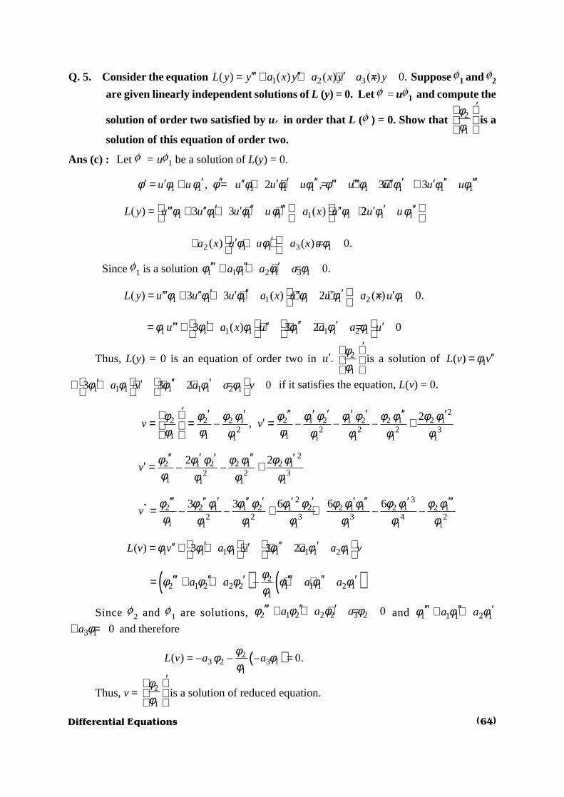
Differential Equations
Q. 5. Consider the equation 1 2 3( ) ( ) ( ) ( ) 0.L y y a x y a x y a x y′′′ ′′ ′= + + + = Suppose f1 and f2
are given linearly independent solutions of L (y) = 0. Let f = uf1 and compute the
solution of order two satisfied by u¢ in order that L (f ) = 0. Show that 2
1
φφ
′
is a
solution of this equation of order two.
Ans (c) : Let f = uf1 be a solution of L(y) = 0.
1 1 1 1 1 1 1 1 1, 2 , 3 3φ φ φ φ φ φ φ φ φ φ φ φ′ ′′ ′ ′′ ′ ′′ ′′′′ ′ ′′ ′ ′′′ ′′′ ′′ ′= + = + + = + + + +u u u u u u u u u
1 1 1 1 1 1 1 1( ) 3 3 ( ) 2φ φ φ φ φ φ φ ′ ′′ ′′′ ′ ′′′′′ ′′ ′ ′′ ′= + + + + + + L y u u u u a x u u u
2 1 1 3 1( ) ( ) 0.φ φ φ ′′+ + + = a x u u a x u
Since f1 is a solution 1 1 1 2 1 3 1 0.a a aφ φ φ φ′′′ ′′ ′+ + + =
1 1 1 1 1 1 2 1( ) 3 3 ( ) 2 ( ) 0.L y u u u a x u u a x uφ φ φ φ φ φ ′ ′′ ′′′′ ′′ ′ ′′ ′ ′= + + + + + =
1 1 1 1 1 1 1 2 13 ( ) 3 2 0u a x u a a uφ φ φ φ φ φ ′ ′′ ′′′′ ′′ ′= + + + + + =
Thus, L(y) = 0 is an equation of order two in 2
1
.′ ′
u
φφ
is a solution of 1( )L v vφ ′′=
1 1 1 1 1 1 2 13 3 2 0a v a a vφ φ φ φ φ ′ ′′ ′′+ + + + + = if it satisfies the equation, L(v) = 0.
2
2 2 2 1 2 1 2 1 2 2 1 2 12 2 2 2 3
1 1 11 1 1 1 1
2– , – – –
φ φ φ φ φ φ φ φ φ φ φ φ φφ φ φφ φ φ φ φ
′ ′ ′ ′′ ′ ′ ′ ′ ′′ ′ ′= = = +
v v
22 1 2 2 1 2 1
2 2 31 1 1 1
2 2– –
′′ ′ ′ ′′ ′′ = +v
φ φ φ φ φ φ φφ φ φ φ
2 3'' 2 2 1 1 2 1 2 2 1 1 2 1 2 1
2 2 3 3 4 21 1 1 1 1 1 1
3 3 6 6 6– – – –
φ φ φ φ φ φ φ φ φ φ φ φ φ φφ φ φ φ φ φ φ
′′′ ′′ ′ ′′ ′ ′ ′ ′ ′′ ′ ′′′= + +v
1 1 1 1 1 1 1 2 1( ) 3 3 2L v v a v a a vφ φ φ φ φ φ ′ ′′ ′′′ ′= + + + + +
( ) ( )22 1 2 2 2 1 1 1 2 1
1
–a a a aφφ φ φ φ φ φφ
′′′ ′′ ′ ′′′ ′′ ′= + + + +
Since f2 and f1 are solutions, 2 1 2 2 2 3 2 0φ φ φ φ′′′ ′′ ′+ + + =a a a and 1 1 1 2 1′′′ ′′ ′+ +a aφ φ φ
3 1 0a φ+ = and therefore
( )23 2 3 1
1
( ) – – – 0.= =L v a aφφ φφ
Thus, v = 2
1
φφ
′
is a solution of reduced equation.
(64)

Differential Equations
EXERCISE
Use the reduction of order method and find the general solution of each of the followingequations. Verify that f1 satisfies the equation.
(a) 21– 0,x y xy y xφ′′ ′ + = = 1 2(Ans. log )y c x c x x= +
(b) 122 2
– 0,y y y xx x
φ′′ ′ + = = 21 2(Ans. )y c x c x= +
(c) 21(2 1) – 4 4 0,φ′′ ′+ + = =x y xy y x
21 2(Ans. (2 –1))y c x c x= +
(d) 21( – ) – ( –1) 0,y x x y x y xφ′′ ′+ = =
3 2–
3 2
1 2 2(Ans. )
x x
ey c x c x dx
x
+
= + ∫
(e)2
11
– – 0,2x
y y y xx
φ ′′ ′+ = =
2–42 2
1 2 3(Ans. )= + ∫
x
ey c x c x dx
x
(f) 2 1 212 3 – 0,′′ ′+ = =x y xy y xφ
1–12
1 2(Ans. )y c x c x= +
Unit 2 : Basis
In the course on linear algebra we learn about a vector space also called as linear spaceand the basis of a linear space. Suppose S is a set of functions with the following property.
If f1, f2 Î S, c1f1 + c2f2 Î S for any two constants c1, c2. Then the set S is called a linear
space of functions. If a linear space of functions S contains n functions 1 2 3, , ,...., nφ φ φ φ which
are linearly independent and every function from S can be represented as a linear combination
of these functions 1 2 3, , ,...., nφ φ φ φ then the set {1 2 3, , ,...., nφ φ φ φ } is called a basis for the linear
space S. The number n is called dimension of S.
For a given linear differential equation ( ) ( –1) ( –1)1 2( ) ( ) ( )n n nL y y a x y a x y= + + + ⋅⋅⋅
( ) 0,na x y+ = the collection of all solutions denoted by S of L(y) = 0 is a linear space. Every
basis of S contains n linearly independent functions and therefore dimension of solution space Sis n.
To check the linear independence of functions 1 2 3, , ,...., nφ φ φ φ , we consider the wronskian
W( 1 2 3, , ,...., nφ φ φ φ ). There is a relation between the linear indepence of functions and the
Wronskian W( 1 2 3, , ,...., nφ φ φ φ ). In chapter I we have proved this result for the linear differentialequation with constant coefficients.
(65)

Differential Equations
A. Linear Independence and Wronskian
In section 1(B) we have seen that for the differential equation ( ) ( –1)1( ) ( )n nL y y a x y= +
( –2)2( ) 0n
na x y a y+ + ⋅⋅⋅ + = there are n linearly independent solutions 1 2 3, , ,...., nφ φ φ φ satisfying
the initial conditions ( –1) ( –1)0 0( ) 1, ( ) 0, .i j
i ix x j iφ φ= = ≠ These linearly independent solutions
is a basis of solution space of L(y) = 0. Every solution of L(y) = 0 can be represented as a linear
combination of these functions 1 2 3, , ,...., nφ φ φ φ .
Theorem 2.2.1
Let 1 2 3, , ,...., nφ φ φ φ be n solutions of L(y) = 0 on I satisfying the initial conditions.
( –1) ( –1)0 0 0( ) 1, ( ) 0, ,i j
i ix x j i x Iφ φ= = ≠ ∈
If f is any solution of L(y) = 0 on I, there are n constants c1, c2, c3,....,cn such that
1 1 2 2 n nc c cφ φ φ φ= + + ⋅⋅⋅ +
Proof :
Let f is any solution of L(y) = 0 on I. Let 0 1, 0 2, 0 3,( ) ( ) ( )x x xφ α φ α φ α′ ′′= = =
( –1)0( )n
nxφ α⋅⋅ ⋅ = for some constants 1, 2, 3, .nα α α α⋅⋅ ⋅
Consider a function 1 1 2 2 3 3 n nψ α φ α φ α φ α φ= + + + ⋅⋅ ⋅ +
Since 1 2, ,...., nφ φ φ are solutions of L(y) = 0, by superposition principle (chapter 2 unit
1(B)) y is also a solution of L(y) = 0 and clearly
0 1 1 0 2 2 0 3 3 0 0 1( ) ( ) ( ) ( ) ( )n nx x x x xψ α φ α φ α φ α φ α= + + + ⋅⋅⋅ + =
as 1 0( ) 1 andxφ = 0( ) 0 for 2,3,4,..., .i x i nφ = =
0 1 1 0 2 2 0 3 3 0 0 2( ) ( ) ( ) ( ) ( )n nx x x x xψ α φ α φ α φ α φ α′ ′ ′ ′′ = + + + ⋅⋅ ⋅+ =
Since, 1 0 2 0 3 0 0( ) 0, ( ) 1, ( ) 0 ( ) 0.nx x x xφ φ φ φ′ ′ ′ ′= = = ⋅⋅ ⋅ =
0 1 1 0 2 2 0 3 3 0 0 3( ) ( ) ( ) ( ) ( )n nx x x x xψ α φ α φ α φ α φ α′′ ′′ ′′ ′′′′ = + + + ⋅ ⋅⋅ + =
Since, 1 0 2 0 3 0 0( ) 0, ( ) 1, ( ) 0 ( ) 0.nx x x xφ φ φ φ′′ ′′ ′′ ′′= = = ⋅⋅⋅ =
In general 0( ) 3,4,5,...., –1iix i nψ α= =
Thus, we see that
( –1)0 1 0 2 0 3 0( ) , ( ) , ( ) ,..., ( ) .n
nx x x xψ α ψ α ψ α ψ α′ ′′= = = =
Thus, y is a solution of L(y) = 0 having the same initial conditions at x0 as that of f . Byuniqueness theorem (chapter II Unit I theorem 2.1.2) we must have y = f .
i.e. 1 1 2 2 3 3 .... n nφ α φ α φ α φ α φ= + + + +
(66)
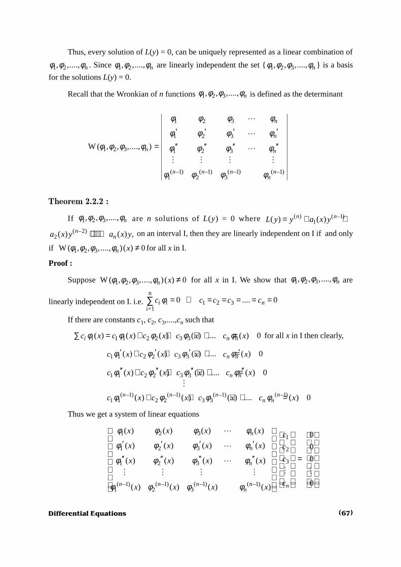
Differential Equations
Thus, every solution of L(y) = 0, can be uniquely represented as a linear combination of
1 2, ,...., nφ φ φ . Since 1 2, ,...., nφ φ φ are linearly independent the set {1 2 3, , ,...., nφ φ φ φ } is a basis
for the solutions L(y) = 0.
Recall that the Wronkian of n functions 1 2 3, , ,...., nφ φ φ φ is defined as the determinant
1 2 3
1 2 3
1 2 3 1 2 3
( –1) ( –1) ( –1) ( –1)1 2 3
W ( , , ,...., )
φ φ φ φ
φ φ φ φφ φ φ φ φ φ φ φ
φ φ φ φ
′ ′ ′ ′
= ′′ ′′ ′′ ′′
L
L
L
M M M M
n
n
n n
n n n nn
Theorem 2.2.2 :
If 1 2 3, , ,...., nφ φ φ φ are n solutions of L(y) = 0 where ( ) ( –1)1( ) ( )n nL y y a x y= + +
( –2)2( ) ( ) ,n
na x y a x y+ ⋅⋅⋅ + on an interval I, then they are linearly independent on I if and only
if 1 2 3W ( , , ,...., ) ( ) 0n xφ φ φ φ ≠ for all x in I.
Proof :
Suppose 1 2 3W ( , , ,...., ) ( ) 0n xφ φ φ φ ≠ for all x in I. We show that 1 2 3, , ,...., nφ φ φ φ are
linearly independent on I. i.e. n
1 2 3i=1
0 .... 0φ = ⇒ = = = = =∑ i i nc c c c c
If there are constants c1, c2, c3,....,cn such that
1 1 2 2 3 3( ) ( ) ( ) ( ) .... ( ) 0i i n nc x c x c x c x c xφ φ φ φ φ∑ = + + + + = for all x in I then clearly,
1 1 2 2 3 3( ) ( ) ( ) .... ( ) 0n nc x c x c x c xφ φ φ φ′ ′ ′ ′+ + + + =
1 1 2 2 3 3( ) ( ) ( ) .... ( ) 0n nc x c x c x c xφ φ φ φ′′ ′′ ′′ ′′+ + + + =M
( –1) ( –1) ( –1) ( –1)1 1 2 2 3 3( ) ( ) ( ) .... ( ) 0n n n n
n nc x c x c x c xφ φ φ φ+ + + + =
Thus we get a system of linear equations
1 2 31
1 2 3 2
31 2 3
( –1) ( –1) ( –1) ( –1)1 2 3
( ) ( ) ( ) ( ) 0( ) ( ) ( ) ( ) 0
0( ) ( ) ( ) ( )
0( ) ( ) ( ) ( )
n
n
n
n n n n nn
x x x x cx x x x c
cx x x x
cx x x x
φ φ φ φ
φ φ φ φ
φ φ φ φ
φ φ φ φ
′ ′ ′ ′ =′′ ′′ ′′ ′′
L
L
L
M MM M M M
(67)

Differential Equations
The above system can be represented by Ax = 0. If A is invertible then we can premultiplyby A–1 and we get x = 0. The square matrix is invertible if it is non-singular i.e. determinant ofA is non-zero.
The determinant of the matrix A is 1 2 3W ( , , ,...., ) ( )n xφ φ φ φ . Therefore if
1 2 3W ( , , ,...., ) ( ) 0n xφ φ φ φ ≠ then c1= c2 = c3 =.... = cn = 0. Since n
i=10 0,i i ic cφ = ⇒ =∑
1,2,3,...., ,=i n 1 2 3, , ,..., nφ φ φ φ are linearly independent.
Conversely, suppose 1 2 3, , ,...., nφ φ φ φ are linearly independent solutions of L(y) = 0 defined
on I. Suppose there is an x0 in I such that 1 2 3 0W ( , , ,...., ) ( ) 0.n xφ φ φ φ =
Then system of n linear equations
1 0 2 0 3 0 01
1 0 2 0 3 0 0 2
31 0 2 0 3 0 0
( –1) ( –1) ( –1) ( –1)1 0 2 0 3 0 0
( ) ( ) ( ) ( ) 0( ) ( ) ( ) ( ) 0
0( ) ( ) ( ) ( )
0( ) ( ) ( ) ( )
n
n
n
n n n n nn
x x x x cx x x x c
cx x x x
cx x x x
φ φ φ φ
φ φ φ φ
φ φ φ φ
φ φ φ φ
′ ′ ′ ′ =′′ ′′ ′′ ′′
L
L
L
M MM M M M
has a solution c1, c2, c3,....,cn, where not all the constants c1, c2, c3,...,cn are zero. Letc1, c2, c3,....,cn be a non-zero solution of above system of equations and consider
1 1 2 2 3 3( ) ( ) ( ) ( ) ( ).n nx c x c x c x c xψ φ φ φ φ= + + + ⋅⋅⋅ +
Since, , 1,2,3....i i nφ = are solution of L(y) = 0, y is also a solution of equation L(y) = 0.
Now L(y) = 0 and from above system of equations we get
0 1 1 0 2 2 0 3 3 0 0( ) ( ) ( ) ( ) ( ) 0n nx c x c x c x c xψ φ φ φ φ= + + + ⋅⋅⋅ + = .
0 1 1 0 2 2 0 3 3 0 0( ) ( ) ( ) ( ) ( ) 0n nx c x c x c x c xψ φ φ φ φ′ ′ ′ ′′ = + + + ⋅⋅ ⋅ + =
In general
( ) ( ) ( ) ( ) ( )0 1 1 0 2 2 0 3 3 0 0( ) ( ) ( ) ( ) ( ) 0i i i i i
n nx c x c x c x c xψ φ φ φ φ= + + + ⋅⋅⋅ + =
for i = 1, 2, 3, 4,...., n –1.
Thus, ( –1)0 0 0 0( ) ( ) ( ) .... ( ) 0.nx x x xψ ψ ψ ψ′ ′′= = = = =
From theorem 2.1.1 it follows that ( ) 0xψ ≡ on I.
Therefore, 1 1 2 2 3 3( ) ( ) ( ) ( ) 0n nc x c x c x c xφ φ φ φ+ + + ⋅⋅⋅ + = for all x in I. Thus, we have c1,
c2, c3,..... cn not all zero such that 1 1 2 2 3 3( ) ( ) ( ) ( ) 0n nc x c x c x c xφ φ φ φ+ + + ⋅⋅⋅ + = for all x in I.
Therefore the set 1 2 3, , ,...., nφ φ φ φ is not linearly independent on I. But this contradicts the fact
that 1 2 3, , ,...., nφ φ φ φ are linearly independent on I. Therefore the assumption that there was a
point x0 in I such that 1 2 3 0W ( , , ,...., ) ( ) 0.n xφ φ φ φ = must be false i.e. 1 2 3W ( , , ,...., ) ( ) 0n xφ φ φ φ ≠for all x in I.
(68)

Differential Equations
Theorem 2.2.3
Let 1 2 3, , ,...., nφ φ φ φ be n linearly independent solutions of ( ) ( –1)1( ) ( )n nL y y a x y= +
( –2)2( ) ( ) 0n
na x y a x y+ + ⋅⋅ ⋅+ = on an interval I. If f is any solution of L(y) = 0 on I, it can be
represented in the form 1 1 2 2 3 3 .... n nc c c cφ φ φ φ φ= + + + + , where c1, c2, c3,..... cn are constants.
Thus any set of n linearly independent solutions of L(y) = 0 on I is a basis for the solution spaceof L(y) = 0 on I.
Proof :
Let x0 be a point in I. Suppose f is any solution of L(y) = 0. Let 0 1, 0 2,( ) ( )x xφ α φ α′= =( –1)
0 3, 0( ) ( )nnx xφ α φ α′′ = ⋅⋅ ⋅ = We show that there exist unique constants c1, c2, c3,..... cn such
that 1 1 2 2 3 3( ) ( ) ( ) ( )n nc x c x c x c xψ φ φ φ φ= + + + ⋅⋅⋅ + is a solution of L(y) = 0 satisfying
( –1)0 1 0 2 0 3 0( ) , ( ) , ( ) ,...., ( ) .ψ α ψ α ψ α ψ α′ ′′= = = =n
nx x x x These initial conditions are
equivalent to the following equations for c1, c2, c3,..... cn (e.g. 0 1 1 0 2 2 0( ) ( ) ( )x c x c xψ φ φ= + +
0 1.... ( )n nc xφ α+ = )
1 0 2 0 3 0 01 1
1 0 2 0 3 0 0 2 2
3 31 0 2 0 3 0 0
( –1) ( –1) ( –1) ( –1)1 0 2 0 3 0 0
( ) ( ) ( ) ( )
( ) ( ) ( ) ( )
( ) ( ) ( ) ( )
( ) ( ) ( ) ( )
φ φ φ φ αφ φ φ φ α
αφ φ φ φ
αφ φ φ φ
′ ′ ′ ′ =′′ ′′ ′′ ′′
L
L
L
M MM M M M
n
n
n
n n n n n nn
x x x x cx x x x c
cx x x x
cx x x x
Since 1 2 3, , ,...., nφ φ φ φ are linearly independent by theorem 2.2.2, 1 2 3W ( , , ,...., )nφ φ φ φ
0( ) 0.x ≠ Therefore the coefficient matrix is inversible and there is a unique solution
c1, c2, c3,..... cn of the above system of equations.Thus we have a unique solution
1 1 2 2 3 3( ) ( ) ( ) ( )n nc x c x c x c xψ φ φ φ φ= + + + ⋅⋅⋅ +
Satisfying ( –1)0 1 0 2 0 3 0( ) , ( ) , ( ) ,...., ( ) .ψ α ψ α ψ α ψ α′ ′′= = = =n
nx x x x But f is a solution
with identical initial conditions. Therefore by uniqueness theorem we have f (x) = y (x) on I.
Thus 1 1 2 2 3 3( ) ( ) ( ) ( ) ( )n nx c x c x c x c xφ φ φ φ φ= + + + ⋅⋅ ⋅ + on I and any solution of L(y) = 0 can
be represented as a linear combination of n linearly independent solutions 1 2 3, , ,...., nφ φ φ φ .
In theorem 2.2.2 we have seen that the function 1 2 3, , ,...., nφ φ φ φ are linearly independent
solutions of L(y) = 0 if and only if the Wronskian 1 2 3W ( , , ,...., ) ( ) 0n xφ φ φ φ ≠ for all x in I. In the
next theorem we show that it is sufficient to calculate the Wronskian 1 2 3W ( , , ,...., )nφ φ φ φ at
some point x0 in I.
(69)

Differential Equations
Theorem 2.2.4
Let 1 2 3, , ,...., nφ φ φ φ be n solutions of L(y) = 0 on an interval I and let x0 be any point in I.
Then
0
1 2 3 1 1 2 3 0W( , , ,..., ) ( ) exp – ( ) W( , , ,..., ) ( )x
n nx
x a t dt xφ φ φ φ φ φ φ φ =
∫
Note that since exponential function is non-zero function,
1 2 3 0W( , , ,..., ) ( ) 0n xφ φ φ φ ≠ implies 1 2 3W( , , ,..., ) ( ) 0n xφ φ φ φ ≠ for all x in I.
Proof :
Let W =
1 2 3
1 2 3
1 2 3 1 2 3
( –1) ( –1) ( –1) ( –1)1 2 3
W ( , , ,...., )
φ φ φ φ
φ φ φ φφ φ φ φ φ φ φ φ
φ φ φ φ
′ ′ ′ ′
= ′′ ′′ ′′ ′′
L
L
L
M M M M
n
n
n n
n n n nn
On differentiating W row wise we get
1 2 31 2 3
1 2 31 2 3
1 2 31 2 3
( –1) ( –1) ( –1) ( –1)( –1) ( –1) ( –1) ( –1)1 2 31 2 3
W ...
φ φ φ φφ φ φ φ
φ φ φ φφ φ φ φ
φ φ φ φφ φ φ φ
φ φ φ φφ φ φ φ
′ ′ ′ ′ ′′ ′′ ′′ ′′ ′ ′ ′ ′ ′ = + +′′ ′′ ′′ ′′′′ ′′ ′′ ′′
LL
LL
LL
M M M MM M M M
nn
nn
nn
n n n nn n n nnn
1 2 3
1 2 3
( –2) ( –2) ( –2) ( –2)1 2 3
( ) ( ) ( ) ( )1 2 3
φ φ φ φ
φ φ φ φ
φ φ φ φ
φ φ φ φ
′ ′ ′ ′ +
L
L
M M M L M
n
n
n n n nn
n n n nn
= V1 + V2 + V3 + ..... + Vn (say)
Where Vk differs from W only in its kth row and the kth row of Vk is obtained bydifferentiating the kth row of W. The first n – 1 determinants are all zero, since they each havetwo identical rows. Observe that Vk has kth and (k + 1)th row identical.
Since 1 2, ,...., nφ φ φ are solution of L(y) = 0, we have
( ) ( –1) ( –2) ( –3)1 2 3– – – .... – ( 1,2,3,..., )n n n n
n ii i i ia a a a i nφ φ φ φ φ= =
(70)

Differential Equations
–1
( )–
0–
nj
n j ij
a φ=
= ∑
Therefore
1 2 3
1 2 3
1 2 3
( –2) ( –2) ( –2) ( –2)1 2 3
–1 –1 –1 –1( ) ( ) ( ) ( )
– – – –1 2 30 0 0 0
W
– – – –
φ φ φ φ
φ φ φ φ
φ φ φ φ
φ φ φ φ
φ φ φ φ= = = =
′ ′
′′ ′′ ′′ ′′ ′ = =
∑ ∑ ∑ ∑
L
L
L
M M M M
L
n
n
n
n
n n n nn
n n n nj j j j
n j n j n j n j nj j j j
V
a a a a
Elimentary row transformations do not change the value of the determinant. Perform thetransformation
1 –1 3 –3 3 2 –1... .n n n n nR a R a R a R a R+ + + + + we get
1 2 3
1 2 3
( –2) ( –2) ( –2) ( –2)1 2 3 1
( –1) ( –1) ( –1) ( –1)1 1 1 2 1 3 1
W
– – – –
′ ′ ′ ′ ′ =
L
L
M M M M
L
L
n
n
n n n n
n n n nna a a a
φ φ φ φ
φ φ φ φ
φ φ φ φ
φ φ φ φ
1 2 3
1 2 3
1 1 1 2 31 2 3
( –1) ( –1) ( –1) ( –1)1 2 3
– – W( , , ,...., )
n
n
nn
n n n nn
a a
φ φ φ φ
φ φ φ φφ φ φ φφ φ φ φ
φ φ φ φ
′ ′ ′ ′ = =′′ ′′ ′′ ′′
L
L
L
M M M M
Therefore W¢ + a1 W = 0 and we get,
10
– ( )
0W( ) W( )∫
=
x
x
a t dt
x e x
i.e. 0
1 2 3 1 1 2 3 0W( , , ,...., ) ( ) exp – ( ) W( , , ,...., ) ( ). =
∫x
n nx
x a t dt xφ φ φ φ φ φ φ φ
Corollatory : If the coefficient a1 is constant then
1 0– ( – )1 2 3 1 2 3 0W( , , ,...., ) ( ) W( , , ,...., ) ( ).a x x
n nx e xφ φ φ φ φ φ φ φ=
From theorem 2.2.2 and theorem 2.2.4 it follows that n solutions 1 2 3, , ,...., nφ φ φ φ of
L(y) = 0 on I are linearly independent if and only if 1 2 3 0W( , , ,..., ) ( ) 0n xφ φ φ φ ≠ for some pointx0 in I.
(71)
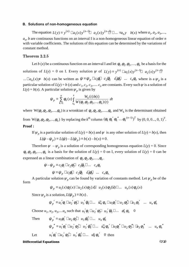
Differential Equations
B. Solutions of non-homogeneous equation
The equation ( ) ( –1) ( –2)1 2( ) ( ) ( ) ... ( )n n n
nL y y a x y a x y a y b x= + + + + = where a1, a2, a3,....,
an, b are continuous functions on an interval I is a non-homogeneous linear equation of order nwith variable coefficients. The solutions of this equation can be determined by the variations ofconstant method.
Theorem 2.2.5
Let b (x) be a continuous function on an interval I and let 1 2 3, , ,...., nφ φ φ φ be a basis for the
solutions of L(y) = 0 on I. Every solution y of ( ) ( –1) ( –2)1 2( ) ( ) ( )= + + +n n nL y y a x y a x y
... ( ) ( )+ =na x y b x can be written as 1 1 2 2 3 3 ...p n nc c c cψ ψ φ φ φ φ= + + + + + where is a yp is a
particular solution of L(y) = b (x) and c1, c2, c3,..... cn are constants. Every such y is a solution ofL(y) = b(x). A particular solution yp is given by
01 1 2 3
( ) ( )( )
( , , ,..., ) ( )ψ φ
φ φ φ φ== ∑ ∫
xnk
p kk nx
W t b tx dt
W t
where 1 2 3W( , , ,..., )nφ φ φ φ is a wronkian of 1 2 3, , ,...., nφ φ φ φ and Wk is the determinant obtained
from 1 2 3W( , , ,..., )nφ φ φ φ by replacing the kth column ( –1)( .... )φ φ φ φ′ ′′ n T
k k k k by (0, 0, 0..., 0, 1)T.
Proof :
If yp is a particular solution of L(y) = b(x) and y is any other solution of L(y) = b(x), then
( – ) ( ) – ( ) ( ) – ( ) 0.p pL L L b x b xψ ψ ψ ψ= = =
Therefore y – yp is a solution of corresponding homogeneous equation L(y) = 0. Since
1 2 3, , ,...., nφ φ φ φ is a basis for the solution of L(y) = 0 on I, every solution of L(y) = 0 can be
expressed as a linear combination of 1 2 3, , ,...., nφ φ φ φ .
1 1 2 2 3 3– ...p n nc c c cψ ψ φ φ φ φ= + + + +
1 1 2 2 3 3 ....p n nc c c cψ ψ φ φ φ φ= + + + + +A particular solution yp can be found by variation of constants method. Let yp be of the
form
1 1 2 2 3 3( ) ( ) ( ) ( ) ( ) ( ) ... ( ) ( )p n nu x x u x x u x x u x xψ φ φ φ φ= + + + +
Since yp is a solution, ( ) ( )pL b xψ = .
1 1 2 2 3 3 1 1 2 2 3 3... ...p n n n nu u u u u u u uψ φ φ φ φ φ φ φ φ′ ′ ′ ′ ′ ′ ′′ ′= + + + + + + + + +
Choose u1, u2, u3,....un such that 1 1 2 2 3 3 ... 0n nu u u uφ φ φ φ′ ′ ′ ′+ + + + =
Then 1 1 2 2 3 3 ...p n nu u u uψ φ φ φ φ′ ′ ′ ′ ′= + + + +
1 1 2 2 3 3 1 1 2 2 3 3... ...p n n n nu u u u u u u uψ φ φ φ φ φ φ φ φ′′ ′ ′ ′ ′ ′ ′ ′ ′′ ′′ ′′ ′′′= + + + + + + + + +
Let 1 1 2 2 3 3 ... 0φ φ φ φ′ ′ ′ ′ ′ ′ ′′+ + + + =n nu u u u then
(72)

Differential Equations
1 1 2 2 3 3 ...p n nu u u uψ φ φ φ φ′′ ′′ ′′ ′′ ′′= + + + +
In general choose ( ) ( ) ( ) ( )1 1 2 2 3 3 ... 0k k k k
n nu u u uφ φ φ φ′ ′ ′ ′+ + + + =
Then ( 1) ( 1) ( 1) ( 1) ( 1)1 1 2 2 3 3 ...k k k k k
p n nu u u uψ φ φ φ φ+ + + + += + + + +
and ( ) ( –1) ( –1) ( –1) ( –1) ( ) ( ) ( )1 1 2 2 3 3 1 1 2 2... ...n n n n n n n n
p n n n nu u u u u u uψ φ φ φ φ φ φ φ′ ′ ′ ′= + + + + + + + +
If we choose ( –1) ( –1) ( –1) ( –1)1 1 2 2 3 3 ... ( )n n n n
n nu u u u b xφ φ φ φ′ ′ ′ ′+ + + + = . Then
( ) ( ) ( ) ( ) ( )1 1 2 2 3 3 ... ( )n n n n n
p n nu u u u b xψ φ φ φ φ= + + + + +Thus we have the following equations
1 1 2 2 3 3 ...p n nu u u uψ φ φ φ φ= + + + +
1 1 2 2 3 3 1 1 2 2 3 3... ; ... 0p n n n nu u u u u u u uψ φ φ φ φ φ φ φ φ′ ′ ′ ′ ′ ′ ′′ ′= + + + + + + + + =
1 1 2 2 3 3 1 1 2 2 3 3... ; ... 0′′ ′′ ′′ ′′ ′′ ′ ′ ′ ′ ′ ′ ′′= + + + + + + + + =p n n n nu u u u u u u uψ φ φ φ φ φ φ φ φ
1 1 2 2 3 3 1 1 2 2 3 3... ; ... 0′′′ ′′′ ′′′ ′′′ ′′′ ′ ′′ ′ ′′ ′ ′′ ′′′= + + + + + + + + =M
p n n n nu u u u u u u uψ φ φ φ φ φ φ φ φ
( –1) ( –1) ( –1) ( –1) ( –2) ( –2)1 1 2 2 1 1 2 2... ;ψ φ φ φ φ φ′ ′= + + + +n n n n n n
p n nu u u u u
( –2) ( –2)3 3 ... 0n n
n nu uφ φ′ ′+ + + =( ) ( ) ( ) ( ) ( ) ( –1) ( –1)
1 1 2 2 3 3 1 1 2 2... ( ) ; ′ ′= + + + + + +n n n n n n np n nu u u u b x u uψ φ φ φ φ φ φ
( –1) ( –1)3 3 ... ( )′ ′+ + + =n n
n nu u b xφ φ
Adding the terms columwise on left we get
1 1 2 2 3 3( ) ( ) ( ) ( ) ... ( ) ( )p n nL u L u L u L u L b xψ φ φ φ φ= + + + + +
Since 1 2 3, , ,...., nφ φ φ φ are n solutions of homogeneous equation L(y) = 0, 1 2( ) ( )L Lφ φ= =
3( ) ... ( ) 0nL Lφ φ= = = and ( ) ( ).pL b xψ =
The right hand side equations are the following system of linear equations.
1 2 3 1
1 2 3 2
1 2 3 3
( –1) ( –1) ( –1) ( –1)1 2 3
0
0
0
φ φ φ φ
φ φ φ φ
φ φ φ φ
φ φ φ φ
′ ′ ′ ′ ′ ′ =′′ ′′ ′′ ′′ ′ ′
L
L
L
MM M M M M
n
n
n
n n n nn n
u
u
u
bu
We solve the above system of equations by Cramer’s rule.
Thus, 1 2 3W( , , ,..., )φ φ φ φ
′ = kk
n
Wu
Where 1 2 3W( , , ,..., )φ φ φ φn is a Wronksian of 1 2 3, , ,...,φ φ φ φn and kW is the determinant
(73)

Differential Equations
obtained from 1 2 3W( , , ,..., )φ φ φ φn by replacing kth column by (0,0,0,.....,0, )Tb . Thus
1 2 –1 1
1 2 –1 1
1 2 –1 1
( –1)( –1) ( –1) ( –1) ( –1)1 2 –1 1
0
0
0
( )
φ φ φ φ φ
φ φ φ φ φ
φ φ φ φ φ
φ φ φ φ φ
+
+
+
+
′ ′ ′ ′ ′
′′ ′′= ′′ ′′ ′′
L L
L
L
M M M M M M
k k n
k k n
k k k n
nn n n nk nk
W
b x
1 2 –1 1
1 2 –1 1
1 2 –1 1
( –1)( –1) ( –1) ( –1) ( –1)1 2 –1 1
0
0
( ) ( )0
1
φ φ φ φ φ
φ φ φ φ φ
φ φ φ φ φ
φ φ φ φ φ
+
+
+
+
′ ′ ′ ′ ′
′′ ′′= =′′ ′′ ′′
L L
L
L
M M M M M M
k k n
k k n
kk k n
nn n n nk nk
b x b x W
Thus, 01 2 3 1 2 3
( ) ( ) ( )i.e. .
W( , , ,..., ) ( , , ,..., ) ( )′ = = ∫
xk k
k kn nx
b x W b t W tu u dt
W tφ φ φ φ φ φ φ φ
and 1 1 2 2 3 31
...ψ φ φ φ φ φ=
= + + + + = ∑n
p n n k kk
u u u u u
01 1 2 3
( ) ( )( ) .
( , , ,..., ) ( )
xnk
kk nx
b t W tx dt
W tφ
φ φ φ φ== ∑ ∫
EXAMPLES
Q. 1. Consider the equation 1 2( ) ( ) ( ) 0,L y y a x y a x y′′ ′= + + = where a1, a2 are continuous onsome interval I. Let f1, f2 and y1, y2 be two bases for the solution L(y) = 0. Show that
there is a non-zero constant k. Such that 1 2 1 2( , ) ( ) ( , ) ( )W x kW xψ ψ φ φ=Ans. : Since f1, f2 is bases for the solutions of L(y) = 0 and y1, y2 are solutions of L(y) = 0.
1 1 1 2 2 2 1 1 2 2and c c d dψ φ φ ψ φ φ= + = +
for some constants c1, c2, d1, d2.
1 1 2 2 1 1 2 21 2
1 1 2 2 1 1 2 2
W( , ) ( )+ +
=′ ′′ ′+ +
c c d dx
c c d d
φ φ φ φψ ψ
φ φ φ φ
1 1 1 1 2 2 2 2 1 1 2 2
1 1 1 1 2 2 2 2 1 1 2 2
c d d c d d
c d d c d d
φ φ φ φ φ φ
φ φ φ φ φ φ
+ += +
′ ′ ′ ′ ′ ′+ +
1 1 1 1 2 2 2 1 1 2 2 2
1 21 1 1 1 2 2 2 1 1 2 2 2
d d d dc c
d d d d
φ φ φ φ φ φ φ φ
φ φ φ φ φ φ φ φ
= + + +
′ ′ ′ ′ ′ ′ ′ ′
(74)

Differential Equations
1 2 2 1
1 2 2 11 2 2 1
c d c dφ φ φ φ
φ φ φ φ
= +
′ ′ ′ ′
1 2
1 2 2 1 1 2 2 1 1 21 2
( – ) ( – ) W( , ) ( )φ φ
φ φφ φ
= =′ ′
c d c d c d c d x
Thus, 1 2 1 2 2 1 1 2W( , ) ( ) ( – ) W( , ) ( )x c d c d xψ ψ φ φ=
Since 1 2,ψ ψ are independent 1 2 2 1– 0.c d c d ≠
Therefore there is a non-zero constant k = c1 d2 – c2 d1 such that 1 2W( , ) ( )xψ ψ =
1 2W( , ) ( ).φ φk x
Q. 2. Consider 1 2( ) ( ) ( ) 0′′ ′= + + =L y y a x y a x y . Show that a1 and a2 are uniquely determinedby any basis f1, f2 for the solutions of L(y) = 0. Show that
1 2 1 2
1 2 1 21 2
1 2 1 2
– , –W( , ) W( , )
a a
φ φ φ φ
φ φ φ φφ φ φ φ
′ ′
′′ ′′ ′′ ′′= =
Ans. : Since f1, f2 is basis for solutions of L(y) = 0 , f1, f2 are solutions of L(y) = 0.
1 1 1 1 2 1( ) 0L a aφ φ φ φ′′ ′= + + =
2 2 1 2 2 2( ) 0L a aφ φ φ φ′′ ′= + + =Solving above two equations for a1 and a2 by Cramers rule, we get.
1 1 1 2
2 2 1 21
1 21 1
2 2
–
––
W( , )
φ φ φ φ
φ φ φ φφ φφ φ
φ φ
′′
′′ ′′ ′′= =
′
′
a
1 1 1 2
2 2 1 22
1 21 1
2 2
–
––
W( , )
′ ′′ ′ ′+
′ ′′ ′′ ′′+= =
′
′
a
φ φ φ φ
φ φ φ φφ φφ φ
φ φ[ We use the elementory properties of determinants det A = det AT and if we interchange
row / column, the value of det change its sign.]
Q. 3. Consider the equation ( ) 0y x yα′′ + = where a is a continuous function on– x∞ < < ∞ .
Let, f1, f2 be the basis for the solutions satisfying
1 2 1 2(0) 1, (0) 0, (0) 1, (0) 1,φ φ φ φ′ ′= = = =
Show that 1 2W( , ) ( ) 1xφ φ = for all x
(75)

Differential Equations
Ans. : For the differential equation
1 2( ) ( ) 0,y a x y a x y′′ ′+ + = if f1 and f2 are two solutions then
10
– ( )
1 2 1 2 0W( , )( ) W( , ) ( )φ φ φ φ∫
=
x
x
a t dt
x e x
For 1( ) 0, 0y x y aα′′ + = = . Therefore 1 2 1 2W( , ) ( ) W( , ) (0)xφ φ φ φ=
1 2
1 2
(0) (0) 1 01
0 1(0) (0)
φ φ
φ φ= = =
′ ′
Thus, 1 2W( , ) ( ) 1xφ φ = for all x.
Q. 4. Find a general solution of 22
– (0 )′′ = < <y y x x ax
Ans. : Assume that the solution of homogeneous equation 22
( ) – 0L y y yx
′′= = is of the form
xr. Then y = xr implies –2 –2( ) ( –1) – 2 0r r rL x r r x x= = gives r (r – 1) – 2 = 0. Then
r2 – r – 2 = 0 implies r = 2 and r = – 1. Thus, f1(x) = x2 and 21
( )xx
φ = are solutions of
homogeneous equation 22
( ) – 0.L y y yx
′′= =
A solution yp of the non-homogeneous equation has the form
1 1 2 2( ) ( ) ( ) ( )p u x x u x xψ φ φ= +
2
1 21
( ) ( )= +u x x u xx
Where, 1 21 2
1 2 1 2
( ) W ( ) Wand
W( , ) W( , )
b x b xu u
φ φ φ φ′ ′= =
Here b (x) = x
22
1 2
2
10
01W – , W
1 2 11 –
xxx
x xx
= = = =
2
1 21 2
1 22
1
W( , ) –1– 2 –31
2 –
φ φφ φ
φ φ= = = =
′ ′
xx
xx
and we find that
( ) 21 32
1 2
– ( ) W ( )1and –
–3 3 W –3 3′ ′= = = = =xx b x x x x
u u
We may take 1 3x
u = and 4
2 – .12x
u = We skip the constants of integration as they correspond
to the solution of corresponding homogeneous equation.
(76)

Differential Equations
Thus, the solution of non-homogeneous equation becomes4 3
2 1– .
3 12 4px x x
xx
ψ = ⋅ ⋅ =
Every solution f of L(y) = x has the form
3
2 21 1 2 2 1( ) ( ) ( )
4pcx
x c x c x c xx
φ ψ φ φ= + + = + +
where, c1 and c2 are constants.
Q. 5. One solution of 2 – 2 0x y y′′ = on 0 < x < ¥ is 21( ) .x xφ = Find all solutions of
2 – 2 2 –1x y y x′′ = on 0 < x < ¥.
Ans. : 21( )x xφ = Let 2 1( ) ( ) ( )x u x xφ φ= be a solution of 2 – 2 0x y y′′ = . Then
22 1 1 1 1( ) ( ) ( ) 2 ( ) ( ) ( ) ( ) – 2 ( ) ( ) 0L x u x x u x x u x x u x xφ φ φ φ φ ′ ′′′′ ′= + + =
2 2 22 ( ) 2 ( ) 2 – 2 ( ) 0x u x u x x u x u x x ′′ ′= + ⋅ + ⋅ =
4 32
4( ) 0 gives 4 0 i.e. –φ ′′′′ ′= + = =
′u
L u x u xu x
–43
1log –4log and or –
3u x u x u
x′ ′= = =
Therefore 2
2 1 31 1
( ) ( ) ( ) – –33
= = ⋅ =x u x x xxx
φ φ
Since L(y) is a linear differential operator 21
( )xx
φ = is a second solution.
Thus, 21( )x xφ = and 2
1( )x
xφ = are solutions of the homogenous equation
2( ) – 2 0L y x y y′′= = or 2– 0y y
x′′ = .
Equation 2 – 2 2 –1x y y x′′ = is the given differential equation. To reduce the equation in
standard form we have to divide the given equation by x2 we can do so since x is positive.
Therefore consider the eqution 2 2
2 2 1– – .y y
xx x′′ = Solution of this equation will be a solution
of given equation.
A solution yp of a non-homogeneous equation 2 2
2 2 1– –y y
xx x′′ = has the form
2
1 1 2 2 1 21
( ) ( ) ( ) ( ) ( ) ( )p u x x u x x u x x u xx
ψ φ φ= + = +
Where, 1 21 2
1 2 1 2
( )W ( )W( ) and ( )
W( , ) W( , )
b x b xu x u x
φ φ φ φ′ ′= =
2
2 1
1 22 1
2 1( ) – , W( , )= –3
2 –x
x
xb x
xx xφ φ= =
(77)

Differential Equations
2
1 22
1 21
0 01W = – , W =
1 – 2 1
x
x
xx
x x= =
2
1 12 3 2
2 1 1– –
2 1 2 1 1 1( ) – and ( ) – – –
–3 3 33 3 2
x xxu x u xxx x x
′ = = =
22
22 2
2 1– ( )
2 1 1 1( ) – and ( ) –
–3 3 3 3 3
′ = = + = +
xx xu x x u x x x
Thus 1 1 2 2( ) ( ) ( ) ( )p u x x u x xψ φ φ= +
22
22 1 1 1
– – – .3 3 3 26
x xx x
x xx
= + + + = +
The general solution of given non-homogeneous equation is 2 21
1– ,
2c
x c xx
ψ = + + + where
c1 and c2 are constants.
Q. 6. One solution of 2 – 0 ( 0)x y xy y x′′ ′ + = > is 1( )x xφ = . Find the solutionsy of
2 2–x y xy y x′′ ′ + = satisfying (1) 1, (1) 0.ψ ψ ′= =
Ans. : The given non-homogeneous equation is 2
1 1– 1.y y y
x x′′ ′ + = (We can divide the equation
by x2 as x2 is positive)
Let 2 1( ) ( ) ( ) ( )x u x x u x xφ φ= = be an other solution.
2 21 1
( ) [ 2 ] – [ ] ( ) 0L u x u u x u u x xx x
φ ′′ ′ ′= + + + = gives 0.u x u′′ ′+ = Therefore 1cux
′ =
and 1( ) log .u x c x=
2 1 1( ) ( ) ( ) logx u x x c x xφ φ= = is second solution. Without loss of generality we choosec1 = 1.
Thus, 1( )x xφ = and 2( ) logx x xφ = are two solutions of homogeneous equation
21 1
– 0.y y yx x
′′ ′ + =
A solution yp of a non-homogeneous equation
2
1 1– 1y y y
x x′′ ′ + = has the form
1 1 2 2( ) ( ) ( ) ( )p u x x u x xψ φ φ= +
Then 1 21 2
1 2 1 2
( )W ( )W( ) , ( )
W( , ) W( , )
b x b xu x u x
φ φ φ φ′ ′= =
(78)

Differential Equations
where 1 2log
( ) 1, W( , )1 1 log
x x xb x x
xφ φ= = =
+
1 20 log 0
W – log , W1 1 log 1 1
x x xx x x
x= = = =
+
1 1– log
( ) – log and ( ) – ( log – )x x
u x x u x x x xx
′ = = =
2 ( ) 1xu x
x′ = = and u2 (x) = x
Therefore 2( – log ) logp x x x x x x x xψ = + ⋅ =
The general solution of given non-homogeneous equation is
21 2 log= + +x c x c x xψ
Since (1) 1ψ = and 1(1) 0, 1 1′ = + =cψ and c1 = 0
2 2 2( ) 2 (log 1), (1) 2 0 and –2′ ′= + + = + = =x x C x c cψ ψTherefore the solution satisfying given initial condition is
2( ) – 2 log .x x x xψ =
Q. 7.
(a) Show that there is a basis f1, f2 for the solutions of 2 24 (2 ) 0 ( 0)′′ ′+ + + = >x y xy x y x
of the form
1 21 22 2
( ) ( )( ) , ( )
x xx x
x x
ψ ψφ φ= =
(b) Find all solutions of
2 2 24 (2 ) for 0x y xy x y x x′′ ′+ + + = > .
Ans. :
(a) Let 2v
xφ = be a solution of the given homogeneous equation.
24 2
( ) 1 0L y y y yx x
′′ ′= + + + =
Then, 2 3 2 3 4
2 4 6– , –
′ ′′ ′′ ′′= = +v v v v v
x x x x xφ φ and
2 3 4 2 3 2 24 6 4 2 2
( ) – – 1 0.v v v v v v
L yxx x x x x x x
′′ ′ ′ = + + + + = Therefore L(y) = 0 implies 0.v v′′ + =
1 2( ) cos and ( ) sinx x x xψ ψ= = are two linearly independent solutions of 0.v v′′ + =
(79)

Differential Equations
Thus, 1 22 2cos sin
( ) and ( )x x
x xx x
φ φ= = are two linearly independent solutions of given
equation.
(b) 1 22 2cos sin
( ) , ( )x x
x xx x
φ φ= =
24 2
( ) 1 1L y y y yx x
′′ ′= + + + = A solution yp of L(y) = 1 has the form
1 1 2 2( ) ( ) ( ) ( ).p u x x u x xψ φ φ= +
Then 1 21 2
1 2 1 2
( )W ( )W( ) , ( )
W( , ) W( , )
b x b xu x u x
φ φ φ φ′ ′= =
where b(x) = 1
2 2
1 2 4
2 3 2 3
cos sin
1W( , )
sin 2cos cos 2sin– – –
x x
x xx x x x x
x x x x
φ φ = =
2 2
1 22 2
2 3 2 3
sin cos0 0
sin cosW – , W
cos 2sin sin 2cos1 – – – 1
= = = =
x x
x xx xx x x xx x
x x x x
2
4
–sin2 2
1 11( ) – sin , ( ) cos – 2 sin – 2cos
xx
x
u x x x u x x x x x x′ = = =
2
4
cos2 2
2 21( ) cos , ( ) sin 2 cos – 2sin′ = = + = +
xx
x
u x x x u x x x x x x
1 1 2 2( ) ( ) ( ) ( )p u x x u x xψ φ φ= +
2 2
2 2cos sin
( cos – 2 sin – 2cos ) ( sin 2 cos – 2sin )x x
x x x x x x x x x xx x
= + +
22
1–x
=
Therefore the general solution of non-homogeneous equation is
1 1 2 2 1 22 2 22 cos sin
1– .px x
c c c cx x x
ψ ψ φ φ= + + = + +
Q. 8. Consider the equation ( )y y b x′′ + = where b is a continuous function on 1 x≤ < ∞
satisfying 1
| ( ) | .b t dt∞
< ∞∫ show that particular solution yp is given by
(80)

Differential Equations
1
( ) sin ( – ) ( )x
p x x t b t dtψ = ∫
Ans. : The homogeneous equation 0y y′′ + = has two solutions 1 2( ) cos , ( ) sin .x x x xφ φ= =
The particular solution yp has the form
1 1 2 2( ) ( ) ( ) ( ) ( )p x u x x u x xψ φ φ= + where
1 2
1 21 1 2 1 1 2
( )W ( )W( ) , ( )
W ( , ) W ( , )
b x b xu x u x
φ φ φ φ′ ′= =
1 2cos sin
W ( , ) 1– sin cos
φ φ = =x x
x x
1 20 sin cos 0
W – sin , W cos1 cos – sin 1
x xx x
x x= = = =
11
1 21 1
( )W ( ) – ( )sin( )
W( , ) ( ) 1
x xb t t b t tu x dt dt
tφ φ= =∫ ∫
22
1 21 1
( )W ( ) ( )cos( )
W( , ) ( ) 1
x xb t t b t tu x dt dt
tφ φ= =∫ ∫
1 1
– cos ( )sin sin ( )cosx x
p x b t t dt x b t t dtψ = +∫ ∫
[ ]1
( ) sin cos – cos sinx
b t x t x t dt= ∫
1
( )sin ( – )x
b t x t dt= ∫
EXERCISE
1. Consider the equation 1 2( ) ( ) 0y a x y a x y′′ ′+ + = where a1(x) and a2(x) are continuous
functions on – ¥ < x < ¥ and are periodic with period q > 0 i.e. 1 1 2( ) ( ), ( )a x a x a xθ θ+ = +
2( )a x= for all x. Let f be a non-trival solution and let ( ) ( )x xψ φ θ= + . Shown that y is
also a solution.
2. Consider the equation ( ) 0y x yα′′ + = where a is a continuous functions on – ¥ < x < ¥which is of period q > 0. Let f1, f2 be the basis for solution satisfying
1 2(0) 1, (0) 0φ φ= =
1 2(0) 0, (0) 1φ φ′ ′= =
Show that there is at least one non-trival solutionf of periodq if and only if 1 2( ) ( ) 2.φ θ φ θ′+ =
(81)

Differential Equations
3. One solution of 2
1( ) 0
4L y y y
x′′= + = for x > 0 is
12
1 ( )x xφ = show that there is another
solution y of the form uψ φ= where u is some function.
4. Use the method of variation of parameter and find the particular solution of the followingequations where the solutions for the related homogeneous equation are given.
(a) 21 22
2 2– log , ( ) , ( )y y y x x x x x x
x xφ φ′′ ′ + = = = 3 3
p1 3
Ans. : log –2 4
x x xψ =
(b)2 3 2
1 2 21
– 4 , ,x y xy y x xx
φ φ′′ ′+ = = = 3
p 5Ans. : xψ =
(c) 2 2 – 11 2– , ,x
xx y xy y x e xφ φ′′ ′+ = = = – –1pAns. : (1 )xe xψ = +
(d)1
22 –1 –11 22 3 – ; ,φ φ′′ ′+ = = =x y xy y x x x
–11p 3Ans. : – logψ = x x
Unit 3 : Homogeneous equations with analytic coefficients
So far we have shown how to construct solutions of various special types of differentialequations using the exponential function, polynomials and the fundamental theorem ofcalculus - that is how to reduce the integration of these differential equations to one or morequadratures. The major difficulty with linear equations with variable coefficients, from a practicalpoint of view, is that it is rare that we can solve equations in terms of elementary functions, suchas exponential and trignometric functions. . However in case the coefficients a1, a2, a3, ...., an,and b have convergent power series expansions the solutions will have this property also andthese series solutions can be obtained by a simple formal process.
An infinite series of the form 00
( – )nnn
a z z∞
=∑ is called a power series in z – z0. Here an, z,
z0 are complex numbers. With every power series there is associated a disk, called the disk ofconvergence such that a series converges absoulately for every z interior to this disk. The centerof the disk is at z0 and its radius is called the radius of convergence of the power series.
Given a power series 00
( – )nnn
a z z∞
=∑ , let Limsup
–11
| | ,nnn a rλ
λ∞= = (where r = 0 if
λ = +∞ and r = ¥ if 0λ = ). The series converges absoulately if 0| – |z z r< and diverges if
0| – | .z z r>
If x0, x and an are real numbers the series 00
( – )nnn
a x x∞
=∑ is called a real power series. Its
disk of convergence intersects the real axis in an interval (x0 – r, x0 + r) called the interval ofconvergence.
If g is a function defined on an interval I containing point x0 we say that g is analytic at x0
if g can be expanded in a power series about x0 which has a positive radius of convergence. Thusg is analytic at x0 if it can be representd in the form
(82)

Differential Equations
00
( ) ( – )nnn
g x a x x∞
== ∑
Where an are constants and the series converges for 0| – | , 0.< >x x r r If g has a power
series expansion then all the derivatives of g exist on 0| – |<x x r and they may be computed bydifferentating the series term by term that is
–1 –2
0 00 0
( ) ( – ) , ( ) ( –1) ( – ) etc.∞ ∞
= =′ ′′= =∑ ∑n n
n nn n
g x n a x x g x n n a x x
The differentiated series converges on 0| – | .x x r<
In calculus there are certain tests by which one could determine an interval of converge ofa real power series. A simple one and one which is frequently used is known as ratio test.
The series 0
in
u∞
=∑ converges absolutely if Lt 1 1.+
→∞ = <nn
n
uk
u
Example 1 : For the power series 0
,∞
=∑
n
n
xn
1
Lt Lt Lim1 1 | |1
++ +
→∞ →∞ →∞= = ⋅ =+
n
n
xn n
n n nxn n
u nx x
u n
Hence the series converges absoulately if | x | < |.
Example 2 : For the power series
–12 4 6
2 –2(–1)1– – .... ....,
2! 4! 6! (2 – 2)!
nnx x x
xn
+ + + +
–12 –2 2
1(–1) (–1)
and (2 – 2)! (2 )!
n nn n
n nu x u xn n+= =
Therefore
2 2
Lim Lim Lim1–1 2 –2
(–1) (2 – 2)!0 for each
(2 )! 2 (2 –1)(–1)+
→∞ →∞ →∞= × = =n n
nn n nn n
n
u x n xx
u n n nx
Hence the series converges absoulately for all x. Its interval of convergence is the entirereal axis.
Theorem 2.3.1 : (Existence theorem)Let x0 be a real number and suppose that the coefficients a1, a2, a3,..... an in
( ) ( –1) ( –2)1 2( ) ( ) ( ) .... ( )n n n
nL y y a x y a x y a x y= + + + +
have convergent power series expansions in powers of (x – x0) on an interval 0| – | , 0.x x r r< >
If a1, a2, a3,.....an are any n constants, there exists a solution f of the problem
( –1)0 1 0 2 0( ) 0, ( ) , ( ) ,...., ( )n
nL y y x y x y xα α α′= = = =
(83)

Differential Equations
with a power series expansion
00
( ) ( – )kkk
x c x xφ∞
== ∑
is convergent for 0| – |x x r< . We have
1! ( 0,1,2,3,...., –1),α += =k kk c k n and ck for k ³ n may be computed in terms of
c0, c1, c2, c3,..... cn – 1 by substituting the series into L(y) = 0.
If the coefficients a1, a2, a3,..... an are analytic at x0 then the solutions are also analytic.The solutions can be computed by a formal algebraic process.
Illustration :
( ) – 0L y y xy′′= =
Here 1 2( ) 0, ( ) –a x a x x= = are analytic for all real x.
Let the solution of the equation L(y) = 0 be f defined by
2 30 1 2 3
0( ) ....φ
∞
== + + + + = ∑ n
nk
x a a x a x a x a x
Then 2 3 –11 2 3 4
1( ) 2 3 4 ....
∞
=′ = + + + + = ∑ n
nn
x a a x a x a x n a xφ
2 –2
2 3 40
( ) 2 6 12 .... ( –1)∞
=′′ = + + + = ∑ n
nn
x a a x a x n n a xφ
–2
2 0( ) – ( ) ( –1) –φ φ
∞ ∞
= =′′ = ∑ ∑n n
n nn n
x x x n n a x x a x
2 3 2 3 42 3 4 5 0 1 2 32 6 12 20 ...– { ...}a a x a x a x a x a x a x a x= + + + + + + + +
2 32 3 0 4 1 5 22 (6 – ) (12 – ) (20 – ) ...= + + + +a a a x a a x a a x
[ ]2 2 –11
2 ( 2) ( 1) – nn n
na n n a a x
∞+
== + + +∑
f is a solutin of ( ) – 0L y y xy′′= = if – 0 orxφ φ′′ =
[ ]2 2 –11
2 ( 2) ( 1) – 0nn n
na n n a a x
∞+
=+ + + =∑
Above equation is true only if all the coefficients of the power series of x are zero. Thus,
2 2 –12 0, ( 2)( 1) – 0, 1,2,3....n na n n a a n+= + + = =
This gives an infinite set of equations, and can be solved for an. Thus, for n = 1 we have
0
3 0 3(3) (2) or (3) (2)
⋅ ⋅ = =⋅
aa a a
For n = 2 we find
1
4 1 4(4) (3) or (4) (3)
⋅ = =⋅
aa a a
(84)

Differential Equations
Continuing in this way we see that
0 1 2
0 1 23 4 5
3 0 4 16 7 8
6 0 7 19 10 11
; 0
; ; 0(3) (2) (4) (3) (5) (4)
; ; 0(6) (5) (6) (5) (3) (2) (7) (6) (7) (6) (4) (3)
; ;(9) (8) (9) (8) (6) (5) (3) (2) (10) (9) (10) (9) (7) (6) (4) (3)
=
= = = =⋅ ⋅ ⋅
= = = = =⋅ ⋅ ⋅ ⋅ ⋅ ⋅ ⋅ ⋅
= = = = =⋅ ⋅ ⋅ ⋅ ⋅ ⋅ ⋅ ⋅ ⋅ ⋅ ⋅ ⋅
a a a
a a aa a a
a a a aa a a
a a a aa a a 0.
In general
0
3 ;(2) (3) (5) (6) (8) (9) (3 –1) (3 )
=⋅ ⋅ ⋅ ⋅ ⋅ ⋅ ⋅ ⋅m
aa
m m
13 1 3 2; 0
(3) (4) (6) (7) (9) (10) (3 ) (3 1)+ += =⋅ ⋅ ⋅ ⋅ ⋅ ⋅ ⋅ ⋅ +m m
aa a
m m
Thus all the constants are determined in terms of a0 and a1. Collecting together termscontaining a0 and a1 as a factor we have
3 6 4 7
0 1( ) 1 ... ...(3) (2) (2) (3) (5) (6) (4) (3) (3) (4) (6) (7)
φ
= + + + + + + + ⋅ ⋅ ⋅ ⋅ ⋅ ⋅ ⋅ ⋅
x x x xx a a x
Let f1 and f2 represent the two series in the brackets.
Thus,3
11
( ) 1 ,2 3 5 6 8 9....(3 –1) (3 )
∞
== +
⋅ ⋅ ⋅ ⋅ ⋅∑m
m
xx
m mφ
3 1
21
( ) .3 4 6 7 9 10....(3 ) (3 1)
φ+∞
== +
⋅ ⋅ ⋅ ⋅ ⋅ +∑m
m
xx x
m m
We have shown, in a formal way that f satisfies – 0y xy′′ = for any two contants a0 and a1
In particular the choice a0 = 0 and a1 = 1 implies f2 (x) satisfies the equation and a0 = 1, a1
= 0 implies f1 (x) satisfies the equation.
The only question that remains is about the convergence of the series, defining f1 (x) andf2 (x).
3
11
( ) 1 ( ) 12 3 5 6 8 9....(3 –1) (3 )
m
mm
xx d x
m mφ
∞
== + = +
⋅ ⋅ ⋅ ⋅ ⋅∑ ∑
3 3
13
2 3 5 6 8 9 (3 –1)(3 )2 3 5 6 8 9 (3 ) (3 2)(3 3)
++ ⋅ ⋅ ⋅ ⋅ ⋅ ⋅⋅ ⋅= ×
⋅ ⋅ ⋅ ⋅ ⋅ ⋅⋅ ⋅ + +
mm
m
d m mxdm m m m x
3
(3 2)(3 3)=
+ +x
m m
Lt sup Lt inf1 10.
(3 2)(3 3) (3 2) (3 3)→∞ →∞= =+ + + +m mm m m m
The series converges if |x | < ¥.
Similarly f2 (x) is convergent series.
(85)

Differential Equations
EXAMPLES
1. Find two linearly independent power series solutions (in powers of x) of the followingequations.
(a) 0y xy y′′ ′− + = (b) 23 – 0y x y xy′′ ′+ =
(c) 2– 0y x y′′ = (d) 3 23 0y x y x y′′ ′+ + =
Ans. (a) : Let 2 30 1 2 3
0( ) ... ...n n
n nn
x a a x a x a x a x a xφ∞
== + + + + + + = ∑ be a solution of
( ) – 0L y y xy y′′ ′= + = . Since it is a solution it satisfies the equation L(f ) = 0.
2 3
0 1 2 30
( ) ... ...n nn n
nx a a x a x a x a x a xφ
∞
== + + + + + + = ∑
Then 2 –1 –11 2 3
1( ) 2 3 ... ...n n
n nn
x a a x a x n a x n a xφ∞
=′ = + + + + + = ∑
–2 –2
2 32
( ) 2 3 2 ... ( –1) ... ( –1)∞
=′′ = + ⋅ + + + = ∑n n
n nn
x a a x n n a x n n a xφ
Thus, –2 –1
2 1 0( ) ( –1) – 0.n n n
n n nn n n
L n n a x x n a x a xφ∞ ∞ ∞
= = == + =∑ ∑ ∑
20 1 0
( 2) ( 1) – 0∞ ∞ ∞
+= = =
= + + + =∑ ∑ ∑n n nn n n
n n nn n a x n a x a x
2 0 21
(2 ) {( 2)( 1) – } 0nn n n
na a n n a na a x
∞+
== + + + + + =∑
2 0 21
( ) (2 ) {( 2)( 1) – ( –1) } 0nn n
nL a a n n a n a xφ
∞+
== + + + + =∑
We see that L(f ) = 0 if and only if 2a2 + a0 = 0 and 2( 2) ( 1) – ( –1) 0++ + =n nn n a n a for
1,2,3,....n = 2 0 2( –1)1
– ;2 ( 2)( 1)
nn
n aa a a
n n+= =+ +
is called recurrence relation.
0 1
02 3 1
024 5
046 7
08 9
010 11
;
–; ; 0.
2 12
– ; .0 04 3 2 3 4 5 4
33– ; 0
6 5 2 3 4 5 63 5
– ; 02 3 4 5 6 7 83 5 7
– ; 010!
= =⋅
= = = =⋅ ⋅ ⋅ ⋅
= = =⋅ ⋅ ⋅ ⋅ ⋅
⋅= =
⋅ ⋅ ⋅ ⋅ ⋅ ⋅⋅ ⋅= =
a a
aa a a
aaa a
aaa a
aa a
aa a
(86)

Differential Equations
In general 2 1 0 1,2,3,....na n+ = =
0
23 5 7 9 (2 – 3)
–(2 )!n
n aa
n
⋅ ⋅ ⋅ ⋅ ⋅⋅=
02 3 4 5 6 7 8 9 (2 – 3) (2 – 2) (2 –1)(2 )
–2 4 6 8 2 (2 –1) (2 )!
n n n na
n n n
⋅ ⋅ ⋅ ⋅ ⋅ ⋅ ⋅ ⋅ ⋅⋅=⋅ ⋅ ⋅ ⋅ ⋅⋅ ⋅
0(2 ) !
–2 !(2 –1)(2 )!n
na
n n n=
0–2 !(2 –1)n
a
n n=
2 2 1
2 2 10 0
( ) n nn n
n nx a x a xφ
∞ ∞ ++
= == +∑ ∑
20
0 11
–2 !(2 –1)
∞
== +∑ n
nn
aa x a x
n n
2
0 11
1–2 !(2 –1)
∞
=
= +
∑
n
nn
xa a x
n n
2
1 21
( ) 1– and ( )2 !(2 –1)
n
nn
xx x x
n nφ φ
∞
== =∑ are two solutions of the equation
Let 10
( ) ( )φ∞
== ∑ m
mx d x
2( 1)
1 21
2
2 ( 1)!(2 1) (2 –1)2( 1) (2 1)
2 !(2 –1)
+
++ + += =
+ +
n
nn
n
n
x
d n n x n
dn n nx
n n
Lt Lt 1 (2 –1)0
2( 1) (2 1)+
→∞ →∞= =+ +
nn n
n
d n
d n nRedius of convergence = ¥The series converges if |x | < ¥ i.e. all values of x. Both the solutions are convergent for
all values of x.
Ans. (b) : Let 0
( )φ∞
== ∑ n
nn
x a x be a solution.
–1 –2
1 2( ) , ( ) ( –1)n n
n nn n
x na x x n n a xφ φ∞ ∞
= =′ ′′= =∑ ∑
2( ) 3 –L x xφ φ φ φ′′ ′= +
(87)

Differential Equations
–2 2 –1
2 1 0( –1) 3 –n n n
n n nn n n
n n a x x n a x x a x∞ ∞ ∞
= = == +∑ ∑ ∑
( ) 0L φ = implies
2 2 3 4 52 3 4 1 2 3 42 1 3 2 4 3 3 2 3 4 ....a a x a x a x a x a x a x ⋅ + ⋅ + ⋅ + ⋅⋅⋅ + + + + +
2 3 40 1 2 3– .... 0.a x a x a x a x + + + + =
[ ] [ ]2 32 3 0 4 1 5 22 1 (3 2 – ) 4 3 (3 –1) 5 4 (3(2) –1)⋅ + ⋅ + ⋅ + + ⋅ +a a a x a a x a a x
[ ] 46 3– 6.5 (3(3) –1) 0a a x+ + ⋅⋅⋅⋅ =
[ ] 12 3 0 3
12 1 (3 2 – ) ( 3) ( 2) (3 –1) 0n
n nn
a a a x n n a n a x∞ +
+=
⋅ + ⋅ + + + + =∑
Then 02 3 3
(3 –1)0 ; ; –
2 3 ( 3) ( 2)n
na n a
a a an n+= = =
⋅ + +
0 1 2
0 13 4 5
3 0 4 16 7 8
0 19 10 11
; ; 0
2– ; – ; 0
2 3 4 3
8 8 11 11 2– ; – ; 0
6 5 2 3 5 6 7 6 7 6 4 3
(18 –1) (9 –1) 20 11 2– ; – ; 0.
9 8 6 5 3 2 10 9 7 6 4 3
a a a
a aa a a
a a a aa a a
a aa a a
=
= = =⋅ ⋅
⋅= = + = = =⋅ ⋅ ⋅ ⋅ ⋅ ⋅ ⋅ ⋅
⋅ ⋅= = =⋅ ⋅ ⋅ ⋅ ⋅ ⋅ ⋅ ⋅ ⋅ ⋅
The solution
31
1
(–1) (–1)8 17 (9 –1)( ) 1
2 3 5 6 8 9 (3 –1) (3 )φ
∞
=
⋅ ⋅⋅ ⋅= +⋅ ⋅ ⋅ ⋅ ⋅ ⋅ ⋅⋅ ⋅
∑m
m
m
mx x
m m
3 12
1
(–1) 2 11 20 (3(3 – 2) –1)( )
3 4 6 7 9 10 (3 )(3 1)φ
∞+
=
⋅ ⋅ ⋅⋅ ⋅= +⋅ ⋅ ⋅ ⋅ ⋅ ⋅⋅⋅ ⋅ +∑
mm
m
mx x x
m m
Ans. (c) : Let 0
( ) nn
nx a xφ
∞
== ∑ be a solution of 2– 0.y x y′′ = Since it is a solution f (x) satisfies
2( ) – 0.L xφ φ φ′′= =
–1 –2
0 1 2( ) , ( ) , ( ) ( –1)n n n
n n nn n n
x a x x n a x x n n a xφ φ φ∞ ∞ ∞
= = =′ ′′= = =∑ ∑ ∑
–2 2
2 0( ) ( –1) – 0.n n
n nn n
L n n a x x a xφ∞ ∞
= == =∑ ∑
–2 22 3
4 02 1 3 2 ( –1) – 0
∞ ∞+
= =⋅ + ⋅ + =∑ ∑n n
n nn n
a a x n n a x a x
(88)

Differential Equations
2 22 3 4
0 02 1 3 2 ( 4) ( 3) – 0
∞ ∞+ +
+= =
⋅ + ⋅ + + + =∑ ∑n nn n
n na a x n n a x a x
Here we have replaced n by n + 4 and therefore the sum is from 0 to ¥.
[ ] 22 3 4
02 1 3 2 ( 4)( 3) – 0.n
n nn
a a x n n a a x∞ +
+=
⋅ + ⋅ + + + =∑
Thus, 2 3 40, 0 and .( 4) ( 3)
nn
aa a a
n n+= = =+ +
0 1 2 3
0 14 5 6 7
0 54 18 9 10 11
0 112 13 14 15
0 0
; ; ; 0 ; 03 4 5 4
; ; 0 ; 08 7 3 4 7 8 9 8 4 5 8 9
; ; 0 ; 03 4 7 8 11 12 4 5 8 9 12 13
a a a a
a aa a a a
a aa aa a a a
a aa a a a
= =
= = = =⋅ ⋅
= = = = = =⋅ ⋅ ⋅ ⋅ ⋅ ⋅ ⋅ ⋅
= = = =⋅ ⋅ ⋅ ⋅ ⋅ ⋅ ⋅ ⋅ ⋅ ⋅M M M M
Thus all the coefficients an’s are determined in terms of a0 and a1 since a2 = a3 = 0 impliesa4m+2 and a4m+3 = 0 for m = 0, 1, 2, 3,..... Therefore
4 1
4 4 10 0
( ) m mm m
m mx a x a xφ
∞ ∞ ++
= == +∑ ∑
4
01
13 4 7 11 12 (4 –1) (4 )
m
m
xa
m m
∞
=
= +
⋅ ⋅ ⋅ ⋅ ⋅⋅⋅ ∑
4 1
114 5 8 9 12 13 (4 ) (4 1)
+∞
=
+ +
⋅ ⋅ ⋅ ⋅ ⋅ ⋅⋅⋅ + ∑
m
m
xa x
m m
Therefore two linearly independent solutions are
4
11
( ) 1 and3 4 7 11 12 13 (4 –1)(4 )
∞
== +
⋅ ⋅ ⋅ ⋅ ⋅ ⋅ ⋅⋅∑m
m
xx
m mφ
4 1
21
( ) .4 5 8 9 12 13 (4 ) (4 1)
m
m
xx x
m mφ
+∞
== +
⋅ ⋅ ⋅ ⋅ ⋅ ⋅⋅⋅ +∑
Ans. (d) : Let 20
( )φ∞
== ∑ n
nn
x a x be a solution of 3 2( ) 0.L y y x y x y′′ ′= + + = Therefore
–2 3 –1 2
2 1 0( ) ( –1) 0φ
∞ ∞ ∞
= = == + + =∑ ∑ ∑n n n
n n nn n n
L n n a x x n a x x a x
that is –2 2 2
2 1 0( –1) 0.
∞ ∞ ∞+ +
= = =+ + =∑ ∑ ∑n n n
n n nn n n
n n a x n a x a x
(89)

Differential Equations
The first term starts from x0 where as last two series start from x3 and x2 respectively. Toget the common base we write the expansion in the following form
2 –2 2 2 22 3 4 0
5 1 12 1 3 2 4 3 ( –1) 0.n n n
n n nn n n
a a x a x n n a x na x a x a x∞ ∞ ∞
+ +
= = =⋅ + ⋅ + ⋅ + + + + =∑ ∑ ∑
Therefore
2 –2 22 3 4 0
5 12 1 3 2 (4 3 ) ( –1) ( 1) 0n n
n nn n
a a x a a x n n a x n a x∞ ∞
+
= =⋅ + ⋅ + ⋅ + + + + =∑ ∑
We replace n by n + 4 in the first series.
[ ]2 22 3 4 0 4
12 1 3 2 (4 3 ) ( 4) ( 3) ( 1) 0.
∞+
+=
⋅ + ⋅ + ⋅ + + + + + + =∑ nn n
na a x a a x n n a n a x
Above equation is true for all values of x and therefore
2 3 4 0 40; 0; 4 3 0; ( 4) ( 3) ( 1) 0+= = ⋅ + = + + + + =n na a a a n n a n a
0 1 2 3
0 14 5 6 7
0 18 9 10 11
0 112 13 14 15
0 0
– –2; ; ; 0 ; 0
3 4 5 45 6 2
; ; 0 ; 03 4 7 8 4 5 8 9
9 5 10 6 2– ; – ; 0 ; 0
3 4 7 8 11 12 4 5 8 9 12 13
= =
= = = =⋅ ⋅
⋅= + = = =⋅ ⋅ ⋅ ⋅ ⋅ ⋅
⋅ ⋅ ⋅= = = =⋅ ⋅ ⋅ ⋅ ⋅ ⋅ ⋅ ⋅ ⋅ ⋅M M M M
a a a a
a aa a a a
a aa a a a
a aa a a a
4(–1) 5 9 13 (4 – 3)
;3 4 7 8 11 12 (4 –1)(4 )
m
mm
am m
⋅ ⋅ ⋅ ⋅⋅=⋅ ⋅ ⋅ ⋅ ⋅ ⋅⋅⋅
4 1 4 2 4 3(–1) 2 6 10 (4 – 2)
; 0.4 5 8 9 (4 ) (4 1)
m
m m mm
a a am m+ + +
⋅ ⋅ ⋅⋅ ⋅= = =⋅ ⋅ ⋅ ⋅⋅ ⋅⋅ +
Therefore two linearly independent solutions are
4
11
(–1) 5 9 13 (4 – 3)( ) 1
3 4 7 8 11 12 (4 –1) (4 )
mm
m
mx x
m mφ
∞
=
⋅ ⋅ ⋅⋅ ⋅= +⋅ ⋅ ⋅ ⋅ ⋅ ⋅ ⋅⋅∑
4 1
21
(–1) 2 6 10 (4 – 2)( )
4 5 8 9 (4 )(4 1)
mm
m
mx x x
m mφ
∞ +
=
⋅ ⋅ ⋅⋅⋅= +⋅ ⋅ ⋅ ⋅⋅ ⋅ +∑
2. Find the solution f of 2( –1) – ( –1) 0y x y x y′′ ′+ = in the form 0
( ) ( –1)kkk
x a xφ∞
== ∑ which
satsfies (1) 1, (1) 0.φ φ′= =
Ans. : Let 0
( ) ( –1)φ∞
== ∑ k
kk
x a x be a solution of 2( ) ( –1) – ( –1) 0.L y y x y x y′′ ′= + =
(90)

Differential Equations
–2 2 –1 1
2 1 0( ) ( –1) ( –1) ( –1) ( –1) – ( –1) 0.k k k
k k kk k k
L k k a x x k a x a xφ∞ ∞ ∞
+
= = == + =∑ ∑ ∑
that is–2 1 1
2 1 0( –1) ( –1) ( –1) – ( –1) 0.k k k
k k kk k k
k k a x k a x a x∞ ∞ ∞+ +
= = =+ =∑ ∑ ∑
–2 12 3
4 12 1 3 2 ( –1) ( –1) ( –1) ( –1)
∞ ∞+
= =⋅ + ⋅ + +∑ ∑k k
k kk k
a a x k k a x k a x
10
1– ( –1) – ( –1) 0k
kk
a x a x∞ +
==∑
In the third term replace k by k + 3 we get
[ ] [ ] 12 3 0 3
12 1 3 2 – ( –1) ( 3) ( 2) ( –1) 0.
∞+
+=
⋅ + ⋅ + + + + =∑ kk k
ka a a x k k a k a x
Thus,
0 1 2
03 4 5
3 06 7 8
6 09 10 11
03 3 1 3 2
; ; 0
; 0 ; 03 2
2 –2– ; 0 ; 0
6 5 2 3 5 6
–5 5 2; 0 ; 0.
9 8 2 3 5 6 8 9
(–1) 2 5 8 (3 –1); 0 for 1,2... ; 0.
2 3 5 6 8 9 (3 –1) (3 ) + +
=
= = =⋅
= = = =⋅ ⋅ ⋅ ⋅
⋅= = = =⋅ ⋅ ⋅ ⋅ ⋅ ⋅
⋅ ⋅ ⋅⋅ ⋅= = = =
⋅ ⋅ ⋅ ⋅ ⋅ ⋅ ⋅⋅
M M M
m
m m m
a a a
aa a a
a aa a a
a aa a a
m aa a m a
m m
Corresponding to the coefficients a0 and a1 we get the following two linearly independentsolutions.
31
1
(–1) 2 5 8 (3 –1)( ) 1 ( –1)
2 3 5 6 8 9 (3 –1) (3 )
mm
m
mx x
m mφ
∞
=
⋅ ⋅ ⋅⋅ ⋅= +⋅ ⋅ ⋅ ⋅ ⋅ ⋅⋅ ⋅∑ and
1( ) ( –1)x xφ =
The general solution f is
3
0 11
(–1) 2 5 8 (3 –1)( ) 1 ( –1) ( –1)
2 3 5 6 (3 –1) (3 )
∞
=
⋅ ⋅ ⋅⋅ ⋅= + + ⋅ ⋅ ⋅ ⋅ ⋅⋅
∑m
m
m
mx a x a x
m mφ
1 0(1) 1 give 1aφ = =
3 –10 1
1
(–1) 2 5 8 (3 –1) (3 )( ) ( –1)
2 3 5 6 (3 –1) (3 )
∞
=
⋅ ⋅ ⋅⋅ ⋅′ = +⋅ ⋅ ⋅ ⋅ ⋅⋅∑m
m
m
m mx a x a
m mφ
1(1) 0 give 0.aφ′ = =
(91)

Differential Equations
Thus, the required solution is
3
1
(–1) 2 5 8 (3 –1)( ) 1 ( –1) .
2 3 5 6 (3 –1)(3 )
mm
m
mx x
m mφ
∞
=
⋅ ⋅ ⋅ ⋅⋅= +⋅ ⋅ ⋅ ⋅⋅⋅∑
3. Compute the solution f of – 0y xy′′′ = which satisfies (0) 1, (0) 0, (0) 0.φ φ φ′ ′′= = =
Ans. : Let 0
( ) nn
kx a xφ
∞
== ∑ be a solution of ( ) – 0.L y y xy′′′= = Then
–3
3 0( ) ( –1) ( – 2) – 0n n
n nn n
L n n n a x x a xφ∞ ∞
= == =∑ ∑
Then –3 13
4 03 2 1 ( –1) ( – 2) – 0n n
n nn n
a n n n a x a x∞ ∞ +
= =⋅ ⋅ + =∑ ∑
In the first sum replace n by n + 4, then
[ ] 13 4
03 2 1 ( 4)( 3)( 2) – 0n
n nn
a n n n a a x∞ +
+=
⋅ ⋅ + + + + =∑
Thus, 3 40 and .( 4) ( 3)( 2)
nn
aa a
n n n+= =+ + +
0 1 2 3
0 1 24 5 6 7
0 1 28 9 10 11
; ; 0
; ; ; 04 3 2 5 4 3 6 5 4
; ; ; 08 7 6 4 3 2 9 8 7 5 4 3 10 9 8 6 5 4
=
= = = =⋅ ⋅ ⋅ ⋅ ⋅ ⋅
= = = =⋅ ⋅ ⋅ ⋅ ⋅ ⋅ ⋅ ⋅ ⋅ ⋅ ⋅ ⋅ ⋅ ⋅ ⋅
a a a a
a a aa a a a
a a aa a a a
012 2 3 4 6 7 8 10 11 12
=⋅ ⋅ ⋅ ⋅ ⋅ ⋅ ⋅ ⋅
aa ; 1
13 3 4 5 7 8 9 11 12 13=
⋅ ⋅ ⋅ ⋅ ⋅ ⋅ ⋅ ⋅a
a ; 214 4 5 6 8 9 10 12 13 14
=⋅ ⋅ ⋅ ⋅ ⋅ ⋅ ⋅ ⋅
aa
;a15 = 0M M M M
0 14 4 1;
2 3 4 6 7 8 (4 – 2) (4 –1) (4 ) 3 4 5 (4 –1) (4 ) (4 1)m ma a
a am m m m m m+= =
⋅ ⋅ ⋅ ⋅ ⋅ ⋅ ⋅⋅ ⋅ ⋅ ⋅⋅⋅ +
24 2 4 3; ; 0
4 5 6 8 9 10 (4 ) (4 1) (4 2)m ma
a am m m+ += =
⋅ ⋅ ⋅ ⋅ ⋅ ⋅⋅⋅ + +
The general solution f (x) of the given equation contains three parameters a0, a1, a2.The solution f (x) becomes
4
01
( ) 12 3 4 6 7 8 (4 – 2) (4 –1)(4 )
m
m
xx a
m m mφ
∞
=
= +
⋅ ⋅ ⋅ ⋅ ⋅ ⋅ ⋅⋅ ∑
4 1
11 3 4 5 7 8 9 (4 –1)(4 ) (4 1)
m
m
xa x
m m m
+∞
=
+ +
⋅ ⋅ ⋅ ⋅ ⋅ ⋅⋅ ⋅ + ∑
(92)

Differential Equations
4 22
21 4 5 6 8 9 10 (4 )(4 1)(4 2)
m
m
xa x
m m m
+∞
=
+ +
⋅ ⋅ ⋅ ⋅ ⋅ ⋅⋅ ⋅ + + ∑
0(0) 1 gives 1aφ = =
(4 –1)
01
4( )
2 3 4 6 7 8 (4 – 2)(4 –1) (4 )
m
m
mxx a
m m mφ
∞
=′ =
⋅ ⋅ ⋅ ⋅ ⋅ ⋅⋅ ⋅∑
4
11
(4 1)1
3 4 5 7 8 9 (4 –1)(4 ) (4 1)
∞
=
++ + ⋅ ⋅ ⋅ ⋅ ⋅ ⋅ ⋅⋅ + ∑
m
m
m xa
m m m
4 1
21
(4 2)2
3 4 5 7 8 9 (4 –1) (4 )(4 1)
+∞
=
++ + ⋅ ⋅ ⋅ ⋅ ⋅ ⋅⋅ ⋅ + ∑
m
m
m xa x
m m m
1(0) 0 gives 0.aφ′ = =
Similarly 2(0) 0 gives 0.aφ′′ = =Thus, the required solution is
4
1( ) 1 .
2 3 4 6 7 8 (4 – 2)(4 –1)(4 )
m
m
xx
m m mφ
∞
== +
⋅ ⋅ ⋅ ⋅ ⋅ ⋅⋅⋅∑
4. Legendre equation is an important differential equation occur in physical problems. Theequation
2( ) (1– ) – 2 ( 1) 0L y x y xy yα α′′ ′= + + =wherea is constant is called Legendre equation.
If we write this equation as
2 2
( 1)2– 0,
1– 1–
xy y y
x x
α α +′′ ′ + =
we see that a1, a2 are given by
1 22 2
( 1)2( ) and ( ) .
1– 1–
xa x a x
x x
α α += =
Both these functions are analytic at x = 0. Indeed, 22
0
1
1–k
kx
x
∞
== ∑ and the series converges
for | x | < |.
Thus, a1(x) and a2(x) have the series expansions. Both there series converge for |x | < | .Thus by existence theorem the solution L(y) = 0 on |x | < | have convergent power seriesexpansions.
Let f be any solution of L(y) = 0 on |x | < |.
Suppose 0
( ) nn
kx a xφ
∞
== ∑ then
2 –2 –1
2 1 0( ) (1– ) ( –1) – 2 ( 1)n n n
n n nn n n
L x n n a x x na x a xφ α α∞ ∞ ∞
= = == + +∑ ∑ ∑
(93)

Differential Equations
–2
2 2 1 0( –1) – ( –1) – 2 ( 1)α α
∞ ∞ ∞ ∞
= = = == + +∑ ∑ ∑ ∑n n n n
n n n nn n n n
n n a x n n a x na x a x
[ ]20
( 2) ( 1) –{ ( –1) 2 – ( 1)} nn n
nn n a n n n a xα α
∞+
== + + + +∑
For f to satisfy L(f ) = 0 we must have all the coefficients of the powers of x equal to zero.
Hence, [ ]2( 2) ( 1) – ( 1) – ( 1) 0, 0,1,2,3,...n nn n a n n a nα α++ + + + = =
This is a recurrance relation which gives an +2 in terms of an.
2( 1) – ( 1)
( 1)( 2)n nn n
a an n
α α+
+ +=+ +
– ( 1) ( – ).
( 1) ( 2)
+ +=+ + nn n
an n
α α
for n = 0 we get
2 0( 1)
–2
a aα α +=
3 1( 2) ( –1)
–2 3
a aα α+=
⋅Similarly,
4 2 5 3
0 1
( 3) ( – 2) ( 4) ( – 3)– ; –
3 4 4 5
( 1) ( 3)( – 2) ( 4)( 2)( –1) ( – 3)2 3 4 2 3 4 5
+ += =⋅ ⋅
+ + + += + = +⋅ ⋅ ⋅ ⋅ ⋅
a a a a
a a
α α α α
α α α α α α α α
In general
2 0( 2 –1) ( 2 – 3) ( 1) ( – 2) ( – 2 2)
(–1)(2 )!
mm
m m ma a
m
α α α α α α+ + ⋅⋅⋅ + ⋅ ⋅⋅ +=
2 1 1( 2 ) ( 2 – 2) ( 2)( – 1)( – 3) ( – 2 1)
(–1)(2 1)!
α α α α α α+
+ + ⋅ ⋅ ⋅ + ⋅ ⋅ ⋅ +=+
mm
m m ma a
m
All the coefficients are determined in terms of a0 and a1 and we have
0 1 1 2( ) ( ) ( )x a x a xφ φ φ= +
where, 21
1
(–1) ( 2 –1)( 2 – 3) ( – 2) ( – 2 2)( ) 1
(2 )!
mm
m
m m mx x
m
α α α α αφ∞
=
+ + ⋅⋅ ⋅ ⋅ ⋅⋅ += + ∑
2 12
1
(–1) ( 2 )( 2 – 2) ( 2) ( –1)( – 3) ( – 2 1)( )
(2 1)!
∞ +
=
+ + ⋅⋅⋅ + ⋅⋅ ⋅ += ++∑
mm
m
m m mx x x
m
α α α α α αφ
Both f1 and f2 are solutions of Legendre equation, corresponding to the choices
0 1 0 11, 0 and 0, 1,c c c c= = = =respectively. They form a basis for the solutions, since
1 2 1 2(0) 1, (0) 0 ; (0) 0, (0) 1φ φ φ φ′ ′= = = =
(94)

Differential Equations
1 21 2 1 2 2 1
1 2
(0) (0)W( , ) (0) (0) (0) – (0) (0) 1
(0) (0)
φ φφ φ φ φ φ φ
φ φ′ ′∴ = = =
′ ′
Since Wronkian 1 2 1 2W( , ) (0), ,φ φ φ φ≠ are linearly independent and therefore forms a basis.
If a is a non-negativ even integer a = 2n, then f1 has only a finite number of non-zeroterms. In this case f1 is a polynomial of degree 2n containing only even powers of x. for example,
1 00, ( ) 1 ( )α φ= = =x p x
2 2
1 2(–1) (2 1)
2, ( ) 1 1– 3 ( )2
α φ α+= = + = =x x x p x
or the recurrance relation
2( 1) – ( 1)
( 1) ( 2)n nn n
a an n
α α+
+ +=+ + implies
2 0 00(0) – 2(3)
–31 2
a a a= =⋅
4 22(3) – 2(3)
03 4
a a= =⋅
with a0 = 1 we get 21 2( ) 1– 3 ( )x x p xφ = =
for a = 4, 2 0 00(0) – 4(5)
–101 2
a a a= =⋅
4 22(3) – 4(5)
3 4a a=
⋅
06 – 20
(–10 )12
a=
014012
a= +
0353
a=
64(5) – 4(5)
5 6a =
⋅ = 0
2 41 0 0
3 5( ) 1–10 with 1
3x a x x aφ = + =
2 41 4
3 5( ) 1–10 ( )
3x x x p xφ = + =
The solution f2 is not a polynomial in this case since none of the coefficients in the seriesof f2 vanish.
A similar situation occurs when a is a positive odd integer n. Then f2 is a polynomial ofdegree n having only odd powers of x and f1 is not a polynomial.
(95)

Differential Equations
for example
(a = 1) 2( 1) – ( 1)
( 1) ( 2)n nn n
a an n
α α+
+ +=+ +
3 11(2) –1(2)
02 3
a a= =⋅
2 1( ) ( )x x p xφ = = (say)
(a = 3) 3 11(2) – 3(4)
2 3a a=
⋅
15
–3
a=
5 33(4) – 3(4)
4 5a a=
⋅ = 0
32 3
5( ) – ( )
3x x x p xφ = = (say)
(a = 5) 3 11(2) – 5 6
2 3a a
⋅=⋅
114
–3
a=
5 33(4) – 5 6
4 5a a
⋅=⋅
118 14
– –20 3
a =
1215
a=
7 55 6 – 5 6
0.6 7
a a⋅ ⋅= =
⋅
3 5
2 514 21
( ) – ( )3 5
x x x x p xφ = + = (say)
Definition : 2.1.3
A polynomial solution pn of degree n of 2(1– ) – 2 ( 1) 0,x y xy n n′′ ′ + + =
Satisfying Pn (1) = 1 is called the nth Legendre polynomial and the differential equation iscalled Legendre equation.
Let f be a polynomial of degree n defined by
2( ) ( –1)
nn
nd
x xdx
φ =
2( ) ( –1)nu x x= implies 2 –1( ) ( –1) 2nu x n x x′ = gives
2( –1) ( ) – 2 ( ) 0x u x n x u x′ =
(96)

Differential Equations
Differentiate this equation (n + 1) times.
First differentiation gives
2( –1) ( ) 2 (1– ) ( ) – 2 ( ) 0x u x x n u x n u x′′ ′+ =Second differentiation gives
[ ] [ ]2( –1) ( ) 2 (1 1) – 2 (1– ) (0 – ) ( ) 0x u x x n u n n u x′′′ ′′ ′+ + + + =
Third differentiation gives
[ ] [ ]2 ( )( –1) 2 (1 1 1) – 2 (2 – ) (1– ) (0 – ) 0.′′′ ′′+ + + + + + =ivx u x n u n n n u
i.e. [ ]2 ( )( –1) 2 (3 – ) – 2 ( – 2) ( –1) 0.ivx u x n u n n n u′′′ ′′+ + + =
In general (n + 1)th differentiation gives
[ ]2 ( 2) ( 1) ( )( –1) 2 (( 1) – ) – 2 1 2 3 4 ... ( –1) 0.n n nx u x n n u n n u+ ++ + + + + + + + =
i.e. 2 ( 2) ( 1) ( )( –1) 2 – ( 1) 0.n n nx u x u n n u+ ++ + = or
2 ( 2) ( 1) ( )(1– ) – 2 ( 1) 0.n n nx u x u n n u+ + + + =
Since 2 ( )( ) ( –1) ( ) ( ),
n nn n
n nd d
x x u x u xdx dx
φ = = =
2(1– ) – 2 ( ) ( 1) ( ) 0x x x n n xφ φ φ′′ ′ + + =
Thus the function 2( ) ( –1)n
nn
dx x
dxφ = is a solution of Legendre equation.
2( –1) ( 1) ( –1)
n nn n n
n nd d
x x xdx dx
= +
–1
–1( –1) ( 1) ( –1) ( 1) ...
= + + + +
n nn n n n
n nd d d
x x x xdxdx dx
( –1) ( – 2)....2 1( 1)= ⋅ + +nn n n x terms containing (x – 1) as factor.
= n ! (x + 1)n + terms containing (x – 1) as factor.Thus, at x = 1,
2( –1) 2 !
nn n
nd
x ndx
= ⋅
Define 21 1( ) ( ) ( –1)
2 ! 2 !
nn
n n n nd
P x x xn n dx
φ= = then Pn (x) is a solution of Legendre
equation witha = n 1(1) 2 ! 1.
2 !n
n nP n
n = ⋅ = Thus, Pn(x) is a Legendre polynomial of degreen.
Supposey is a polynomial solution of Legendre equation with a = n. Since f1 and f2 are
basic solutions of Legendre equation 1 1 2 2c cψ φ φ= + on |x | < | for some constants c1 and c2 is
a solution. If n is even f1 is polynomial solution and f2 is not a polynomial 1 1–cψ φ is polynomial
(97)

Differential Equations
where as c2 f2 is not a polynomial and therefore c2 = 0. In particular the function Pn satisfies
1 1( ) ( )nP x c xφ= for some constant c1 if n is even. Since 1 1(1) 1 (1)nP c φ= = therefore 1(1) 0.φ ≠Thus no nontrivial polynomial solution of Legendre equation can be zero at x = 1. A similarresult is valid for n odd.
The formula
21( ) ( –1)
2 !=
nn
n n nd
P x xn dx
is known as Rodriges formula. This expression can be used to prove properties of Legendrepolynomials.
EXERCISES
1. The equation 2 2(1– ) – 0x y xy yα′′ ′ + = where a is a constant is called the Chebyshev
equation.
(a) Compute two linearly independent series solutions for |x | < |.
(b) Show that for every non negative integer a = n there is a polynomial solution of degree n.
2. The equation – 2 2 0,y xy yα′′ ′ + = where a is a constant, is called the Hermite equation.
(a) Find two linearly independent solutions on – ¥ < x < ¥.
(b) Show that there is a polynomial solution of degree n, in case a = n is a non-negativeinteger.
3. Find the general solution valid near the origin
(i) 3 3 0y xy y′′ ′+ + = (ii) 2(1 4 ) – 8 0x y y′′+ =
(iii) 2(1 ) – 4 6 0x y xy y′′ ′+ + = (iv) 2 – 4 0y xy y′′ ′+ =
(v) 2 0y x y′′ + =
Answers :
1. (a)2 2 2 2 2
21
1
(– ) (2 – ) (2 – 2) –( ) 1
(2 )!m
m
mx x
m
α α αφ
∞
=
⋅⋅ ⋅ = + ∑
2 2 2 2 2 22 1
21
(1 – ) (3 – ) (2 –1) –( )
(2 1)!m
m
mx x x
m
α α αφ
∞ +
=
⋅⋅ ⋅ = ++∑
(b) f1 is a polynomial if a is an even integer,
f2 is a polynomial if a is an odd integer.
(98)

Differential Equations
2. (a) 21
1
2 (– ) (2 – ) (2 – 2 – )( ) 1
(2 )!
∞
=
⋅⋅ ⋅= + ∑m
m
m
mx x
m
α α αφ
2 12
1
2 (1– ) (3 – ) (2 –1– )( )
(2 1)!
mm
m
mx x x
m
α α αφ∞ +
=
⋅⋅ ⋅= ++∑
(b) f1 is a polynomial if a is an even integer, f2 is a polynomial if a is an odd integer.
3. (i) 2
01
(–3)( ) 1
2 !
k k
kk
xy x a
k
∞
=
= +
∑
2 1
11
(–3)3 5 7, (2 1)
k k
m
xa x
k
+∞
=
+ +
⋅ ⋅ ⋅⋅ ⋅ + ∑
(ii)1 2 2 1
20 1 2
0
(–1) 2(1 4 )
4 –1
k k k
k
xy a x a
k
+ +∞
== + + ∑
(iii)3
20 1( ) (1– 3 ) –
3x
y x a x a x
= +
(iv)2 1
2 40 1 2
0
3(–1)1( ) 1
12 2 !(2 – 3) (2 –1) (2 1)
+∞
=
= + + + +∑
k k
kk
xy x a x x a
k k k k
(v)4
0 21
(–1)( ) 1
2 ! 3 7 11 (4 –1)
k k
kk
xy x a
k k
∞
=
= +
⋅ ⋅ ⋅ ⋅⋅ ∑
4 1
1 21
(–1)
2 ! 5 9 13 (4 1)
k k
kk
xa x
k k
+∞
=
+ +
⋅ ⋅ ⋅ ⋅⋅ + ∑
S
(99)

Differential Equations
Linear Equations withRegular Singular Points
Chapter 3
Contents :
Unit 1 : Euler equation
Unit 2 : Second order equations with regular singular pointsUnit 3 : The Bessel equationUnit 4 : Regular singular points at infinity
Introduction
For a linear differential equation ( ) ( –1) ( –2)0 1 2( ) ( ) ( ) .... ( ) 0,n n n
na x y a x y a x y a x y+ + + + =where the coefficient functions a0, a1, a2, a3,..... an are analytic at some point x0, the point x0 iscalled an ordinary point of the equation if a0 (x0) ¹ 0. In the last chapter we have obtain powerseries solutions valid near an ordinary point of a linear equation.
A singular point of the above linear equation is any point x = x1 for which a0 (x1) = 0. Inthis chapter we shall get power series solutions valid near a certain kind of singular points of theequation. It is usually difficult to determine the nature of the solutions in the vicinity of singularpoints. However there is a large class of equations for which the singularity is rather weak in thesense that slight modification of the methods used for solving equations with analytic coefficientsdiscussed in chapter II unit 3, serve to yield solutions near the singularities.
Definition 3.1.1 (a)
A point x = x0 is a regular singular point of ( ) ( –1) ( –2)0 1 2( ) ( ) ( ) ( )n n nL y a x y a x y a x y= + +
( ) 0na x y+ ⋅⋅⋅ + = if the equation can be written in the form ( )0 1( ) ( – ) ( )n nL y x x y b x= +
( –1) ( –1)0( – ) ( ) 0+ ⋅⋅⋅ + =n n
nx x y b x y where b1, b2, b3,..., bn are analytic at x0.
If the functions b1, b2, b3,..., bn can be written in the form
0( ) ( – ) ( )β= kk kb x x x x k = 1, 2, 3,.......,n
Where b1, b2, b3,..., bn are analytic at x0 then L(y) = 0 becomes
( ) ( –1) ( –2)1 2( ) ( ) ..... ( ) 0β β β+ + + + =n n n
ny x y x y x y
(100)

Differential Equations
Definition 3.1.1 (b)
A equation of the form ( ) –1 ( –1) ( –2)0 0 1 0 2 0( ) ( – ) ( ) ( – ) ( ) ( – )+ +n n n y nc x x x y c x x x y c x x x
( –2) .... ( ) 0nny c x y+ + = has a regular singular point at x0 if c0, c1, c2, c3,..... cn are analytic at
x = x0 and c0(x0) ¹ 0.
Definition 3.1.2
If x = x0 is a singular point but is not a regular singular point, then it is called irregularsingular point. For example, consider the equation
2 3– – 0.
4x y y y′′ ′ =
The origin x = 0is a singular point but not regular therefore x = 0 is irregular singularpoint. The coefficient of y¢ is not of the form xb1(x) where b1(x) analytic.
In the first unit we study the differential equation that has a regular singular point at originand all the analytic functions b1, b2, b3,..., bn are constants.
Unit 1 : The Euler Equation
The simplest example of a second order equation that follows defination 3.1.1(a) is theEuler equation
2( ) 0L y x y a x y b y′′ ′= + + =where a, b are constants.
Theorem 3.1.1
Consider the second order Euler equation
2( ) 0 ( , constants),L y x y a x y b y a b′′ ′= + + =and the polynomial q given by
( ) ( –1)q r r r ar b= + +A basis for the solutions of the Euler equation on any interval not containing x = 0 is given
by
1 21 2( ) | | , ( ) | | ,r rx x x xφ φ= =
in case r1, r2 are distinct roots of q and by
1 11 2( ) | | , ( ) | | log| |,r rx x x x xφ φ= =
if r1 is a root of equation q of multiplicity two.
Proof :
Case 1 : r1 ¹ r2
(a) We first consider the equation for x > 0. Let xr be a solution of Euler equation
2( ) 0L y x y a x y b y′′ ′= + + =
2 –2 –1( ) ( –1) 0r r r rL x x r r x a x rx bx = + + =
(101)
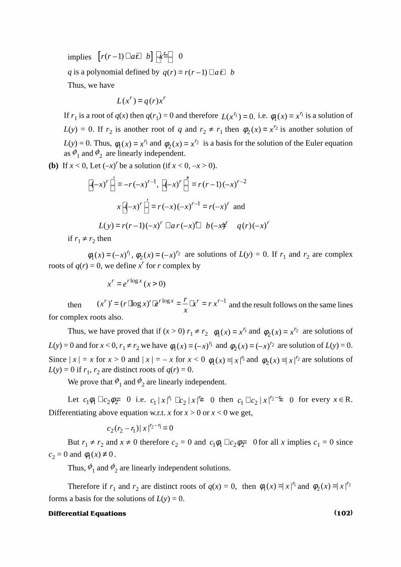
Differential Equations
implies [ ]( –1) 0rr r ar b x + + = q is a polynomial defined by ( ) ( –1)q r r r a r b= + +
Thus, we have
( ) ( )r rL x q r x=
If r1 is a root of q(x) then q(r1) = 0 and therefore 1( ) 0.rL x = i.e. 11( ) rx xφ = is a solution of
L(y) = 0. If r2 is another root of q and r2 ¹ r1 then 22( ) rx xφ = is another solution of
L(y) = 0. Thus, 11( ) rx xφ = and 2
2( ) rx xφ = is a basis for the solution of the Euler equationas f1 and f2 are linearly independent.
(b) If x < 0, Let (–x)r be a solution (if x < 0, –x > 0).
–1 –2(– ) – (– ) , (– ) ( –1) (– )′ ′′ = = r r r rx r x x r r x
–1(– ) (– )(– ) (– )r r rx x r x x r x′ = = and
( ) ( –1)(– ) (– ) (– ) ( )(– )r r r rL y r r x a r x b x q r x= + + =if r1 ¹ r2 then
1 21 2( ) (– ) , ( ) (– )r rx x x xφ φ= = are solutions of L(y) = 0. If r1 and r2 are complex
roots of q(r) = 0, we define xr for r complex by
log ( 0)r r xx e x= >
then log –1( ) ( log )r r x r rr
x r x e x r xx
′ ′= ⋅ ⋅ = ⋅ = and the result follows on the same lines
for complex roots also.
Thus, we have proved that if (x > 0) r1 ¹ r2 11( ) rx xφ = and 2
2( ) rx xφ = are solutions of
L(y) = 0 and for x < 0, r1 ¹ r2 we have 11( ) (– )rx xφ = and 2
2( ) (– )rx xφ = are solution of L(y) = 0.
Since |x | = x for x > 0 and |x | = – x for x < 0 11( ) | |rx xφ = and 2
2( ) | |rx xφ = are solutions ofL(y) = 0 if r1, r2 are distinct roots of q(r) = 0.
We prove that f1 and f2 are linearly independent.
Let 1 1 2 2 0c cφ φ+ = i.e. 1 21 2| | | | 0r rc x c x+ = then 2 1–
1 2 | | 0r rc c x+ = for every x ÎR.
Differentiating above equation w.r.t. x for x > 0 or x < 0 we get,
2 1–2 2 1( – )| | 0r rc r r x =
But r1 ¹ r2 and x ¹ 0 therefore c2 = 0 and 1 1 2 2 0c cφ φ+ = for all x implies c1 = 0 since
c2 = 0 and 1( ) 0xφ ≠ .
Thus, f1 and f2 are linearly independent solutions.
Therefore if r1 and r2 are distinct roots of q(x) = 0, then 11( ) | |rx xφ = and 2
2( ) | |rx xφ =forms a basis for the solutions of L(y) = 0.
(102)

Differential Equations
Case 2 : r1 = r2
(a) x > 0 : If r1 = r2 then q(r1) = 0 and q¢ (r1) = 0. We have proved that if r1 is a root of q(x) = 0
then 1( ) rx xφ = is a solution. To construct second solution consider
( ) ( )∂ ∂ = ∂ ∂
r rL x q r xr r
[ ]( ) ( ) log′= + rq r q r x x
Since, log∂ =∂
r rx x xr
But if r1 = r2 = r then q (r) = 0 and q¢ (r) = 0 and we have
( ) 0∂ = ∂
rL xr
.
( ) ( log )∂ ∂ = = ∂ ∂
r r rL x L x L x xr r
Thus, ( log ) 0rL x x = implies xr log x is a solution of L(y) = 0.
If r1 is a root of q (r) = 0 of multiplicity two then 11( ) rx xφ = and 1
2( ) logrx x xφ = are twosolutions of L(y) = 0.
(b) x < 0 : If x < 0, then – x > 0 and 11( ) (– )rx xφ = and 1
2( ) (– ) log (– )φ = rx x x are solution of
L(y) = 0.
Thus 1 11 2( ) | | and ( ) | | log | – |= =r rx x x x xφ φ are two solution of L(y) = 0.
1 1 2 2 0c cφ φ+ = implies c1 + c2 log |x | = 0 for all x and therefore c1 = c2 = 0 and f1, f2 are
linearly independent.
Thus if r1 is a repeated root of q(r) = 0 then 1 11 2( ) | | and ( ) | | log | |φ φ= =r rx x x x x is a
basis for solutions of the Euler equation 2( ) 0.L y x y a xy by′′ ′= + + =Illustration :
2 0x y xy y′′ ′+ + = for x ¹ 0 is Euler equation with a = b = 1.
The polynomial 2( ) ( –1) 1 1q r r r r r= + + = + and r = +i, – i are roots of q(r). A basis for
the solutions by theorem 3.1.1 are
–1 2( ) | | and ( ) | | ( 0)φ φ= = ≠i ix x x x x
log| || | cos(log | |) sin(log | |)= = +i i xx e x i x
Thus 1( ) cos (log | |)x xψ = and 2( ) sin (log | |)x xψ = is another basis for solution of2( ) 0.′′ ′= + + =L y x y xy y
Theorem 3.1.2Consider the Euler equation of order n.
( ) –1 ( –1) –2 ( –2)1 2( ) ... 0,= + + + + =n n n n n n
nL y x y a x y a x y a y
(103)

Differential Equations
where a1, a2, a3,..., an are constants. Let r1, r2,..., rs be distinct roots of the indicial polynomial
1( ) ( –1) ( – 2)...( – 1) ( –1)...( – 2) ... nq r r r r r n a r r r n a= + + + + + and suppose
ri has multiplicity mi. Then the n functions
1 1 1 1 2 2 2 2–1 –1| | , | | log | |,....,| | (log | |) ; | | ,| | log | |,...,| | (log | |) ;...;r r r m r r r mx x x x x x x x x x
–1| | , | | log | |,...., | | (log | |)s s s sr r r mx x x x x
form a basis for the solution of L(y) = 0 on any interval not containing zero.
Proof : Let |x |r be a solution of L(y) = 0.
–1 –2(| | ) | | , (| | ) ( –1) | | ,....r r r rx r x x r r x′ ′′= =( ) –(| | ) ( –1)( – 2)...( – 1)| |r n r nx r r r r n x= +
Hence, 1(| | ) ( –1) ( – 2)...( – 1)| | ( –1) ( – 2)r rL x r r r r n x a r r r= + +
...( – 2) | | ... | |r rnr n x a x+ + +
( ) | |= rq r x
where 1( ) ( ) ( –1) ( – 2)...( – 1) ( –1)( – 2)...( – 2) ... .= + + + + + nq r r r r r n r r r r n a a
The polynomial q(r) is called indicial polynomial. Thus, |x |r is a solution of L(y) = 0 ifq (r) = 0 i.e. if r is a root of indicial polynomial then |x |r is a solution of L(y) = 0.
Differentiating (| | ) ( ) | |r rL x q r x= with respect to ‘r ’ we get
(| | ) | |r rL x L xr r
∂ ∂ = ∂ ∂ ( )( ) ( ) log | | | |rq r q r x x′= +
In general k times differentiation gives
(| | ) | |k k
r rk k
L x L xr r
∂ ∂= ∂ ∂
( ) ( –1) ( –2) 2( ) ( ) log | | ( –1) ( ) (log | |) ... ( ) (log | |) | | .k r k k rq r kq r x k k q x x q r x x = + + + +
If r is a root of q (r) with multiplicity (k + 1) then ( ) 0, ( ) 0, ( ) 0...,q r q r q r′ ′′= = =
( ) ( ) 0kq r = and therefore | | 0 for 1,2,3,...., .i
ri
L x i kr
∂ = = ∂
Thus ( ) | | , 1,2,3,...., .i
ri
x x i kr
φ ∂= =∂
are solution of L(y) = 0.
If r1 is a root of q(r) of multiplicity m1 then1
1 1 1 1 1 1
1
–122
2 –11 1 1
| | , | | | | log | |, | | | | (log| |) ,..., | |m
r r r r r rm
x x x x x x x xr r r
∂ ∂ ∂= =∂ ∂ ∂
1 1–1| | (log | |)r mx x= are solutions of L(y) = 0.
Repeating this process for each root of q(r) we obtain all the solution and the result follows.All these solutions are linearly independent and therefore form a basis for the solutions of
L(y) = 0 on any interval not containing zero.
(104)

Differential Equations
EXAMPLES
Q. 1. Find all solutions of the following equations for x > 0
(a) 2 2 – 6 0x y xy y′′ ′+ = (b) 22 – 0′′ ′+ =x y xy y
(c) 2 – 4 0x y xy y′′ ′+ = (d) 2 3– 5 9x y xy y x′′ ′ + =
(e) 3 22 – ' 0.′′′ ′′+ + =x y x y xy y
Ans.:
(a) The indicial equation
2( ) ( –1) 2 – 6 – 6q r r r r r r= + = + has root r = 3, – 2.
Therefore 31( )x xφ = and –2
2( )x xφ = are basic solutions and 3 –21 2( )φ = +x c x c x
is general solution for constants c1, c2.
(b) The indicial equation2( ) 2 ( –1) –1 2 – –1q r r r r r r= + = has root r = 1, 1
2– and
1–
21 2( ) , ( )x x x xφ φ= =
are basic solution, 1
–2
1 2( )x c x c xφ = + is general solution for constants c1, c2.
(c) The indicial equation2( ) ( –1) – 4 – 4q r r r r r= + = has root 2, – 2 Then 2
1( )x xφ = and –22( )x xφ = are
basic solution, 2 –21 2( )x c x c xφ = + is general solution.
(d) The indicial equation2( ) ( –1) – 5 9 – 6 9= + = +q r r r r r r has root 3, 3. Since the root 3 is repeated root
of multiplicity two 31( )x xφ = and 3
2( ) logx x xφ = are basic solution of
corresponding homogeneous equation 2 – 5 9 0.x y xy y′′ ′ + = The particular solution will be determined by using variation of constant method.
Let 1 1 2 2( ) ( ) ( ) ( )u x x u x xψ φ φ= + be a solution of equation
25 9
–y y y xx x
′′ ′ + = then
1 2
W ( ) ( )( )
W( , )φ φ= ∫ k
kt b t dt
u x Here b(t) = t,
3 35
1 2 2 2 2
logW ( , ) ,
3 3 logφ φ = =
+
x x xx
x x x x
33
1 2 2
0 logW – log ,
1 3 log
x xx x
x x x= =
+
(105)

Differential Equations
33
2 2
0W ,
3 1= = +
xx
x
32
1 5
– log log 1( ) – – (log )
2x x x x
u x dx dx xxx
⋅= = =∫ ∫
3
2 5( ) log
⋅= = =∫ ∫x x dx dx
u x xxx
1 1 2 2( ) ( ) ( ) ( ) ( )x u x x u x xψ φ φ= +
2 3 3 3 21 1– (log ) (log ) log (log )
2 2x x x x x x x= + =
The general solution
3 3 3 2
1 1 2 2 1 21
log (log ) .2
c c c x c x x x xφ φ φ ψ= + + = + +
(e) The indicial equation
( ) ( –1) ( – 2) 2 ( –1) – 1= + +q r r r r r r r
2 2( –1) – 2 2 –1 ( –1) ( –1)r r r r r r = + = has root 1, 1, –1.
Since one is a root of multiplicity two, 1 2( ) , ( ) logx x x x xφ φ= = and corresponding
to –1, –13( )φ =x x .
The general solution
–11 2 3( ) log .x c x c x x c xφ = + +
Q. 2. Find all solutions of the following equations for | | 0.>x
(a) 2 4 1x y xy y′′ ′+ + = (b) 2 – 3 5 0x y xy y′′ ′ + =
(c) 2 – 4′′ ′+ =x y xy y xπAns.:
(a) The indicial equation ( ) ( –1) 4q r r r r= + + has root 2= ±r i .
Since both the roots are distinct, 21( ) | | ix xφ = and –2
2 ( ) | | ix xφ = . The generalsolution of homogeneous equation is
2 –21 2( ) | | | |i ix c x c xφ = +
The particular solution will be calculated by variation of constant method.
Case 1 : x > 0,If x > 0 then |x | = x
2 –21 2( ) and ( )i ix x x xφ φ= =
Let 1 1 2 2( ) ( ) ( ) ( ) ( )x u x x u x xψ φ φ= + be a solution of
(106)

Differential Equations
2 4 1.x y xy y′′ ′+ + = then 11
1 2
W ( ) ( )( ) and
W( , )
x b x dxu x
φ φ= ∫
22 2
1 2
W ( ) ( ) 1( ) where ( ) ,
W( , )
x b xu x dx b x
xφ φ= =∫
2 –2–1 –1
1 2 2 –1 –2 –1
4W( , ) –2 – 2 –
2 –2
i i
i i
x x ii x i x
xi x ixφ φ = = =
–2 2–2 2
1 2–2 –1 2 –1
0 0W ( ) – ; W
1 –2 2 1
i ii i
i i
x xx x x
ix i x= = = =
–2–2 –2 1 –2 –22
1
1–
( )4 4 4 (–2 ) 8
–
ii i ix
x x xxu x dx dxi i i i
x
+ = = = =
∫ ∫
22 –2 1 2 22
2
1
( ) .4 – 4 – 4 ( 2 ) 8
–
+ = = = =
+
∫ ∫
ii i ix
x x xxu x dx dxi i i i
x
Thus, –2 2
2 –21 1 2 2
1( ) ( ) ( ) ( ) ( )
8 8 4
i ii ix x
x u x x u x x x xψ φ φ= + = ⋅ + ⋅ = . For x > 0,
21( ) ix c xφ = –2
214
ic x+ + is a solution of given equation.
Case 2 : x < 0
If x < 0 then | | –x x= and 2 –21 2( ) (– ) and ( ) (– )i ix x x xφ φ= =
Let 1 1 2 2( ) ( ) ( ) ( ) ( )x u x x u x xψ φ φ= + be a solution of the given differential equation.
2 –2
1 2 2 –1 –2 –1
(– ) (– ) 2 2 4W( , )
(– ) (– ) ––2 (– ) 2 (– )φ φ = = + =
+
i i
i i
x x i i i
x x xi x i x
–2 2–2 2
1 2–2 –1 2 –1
0 (– ) (– ) 0W –(– ) , W (– ) ,
1 2 (– ) –2 (– ) 1
+= = = =i i
i ii i
x xx x
i x i x
21
( )b xx
=
–22 –2 –2
11
1 2
1–(– )
W ( ) ( ) ( ) (– ) (– )1( ) – .
4W( , ) 4 2 8(– )
⋅+= = = =∫ ∫
ii i
xx b x x x x
u x dx dxi i ix
φ φ
(107)

Differential Equations
2
2 2 22
21 2
(– )
W ( ) ( ) (– ) (– ) (– )1( )
4W( , ) 4 –2 8(– )
+ += = = =∫ ∫
i
i ix
x b x x x xu x dx dx
i i ix
φ φ
1 1 2 2( ) ( ) ( ) ( ) ( )x u x x u x xψ φ φ= +
–2 2
2 –2(– ) (– ) 1( ) (– ) (– )
8 8 4= ⋅ + = ⋅
i ii ix x
x x xψ
for x < 0, 2 –21 2
1( ) (– ) (– )
4i ix c x c xφ = + + is a solution of the given differential equation.
Thus 2 –21 2
1( ) | | | |
4i ix c x c xφ = + + is a solution of the given differential equation if x ¹ 0.
(b) The indical equation ( ) ( –1) – 3 5q r r r r= + has roots 2 + i, 2 – i. Since both the roots are
distinct 2 2–1 2( ) | | and ( ) | |φ φ+= =i ix x x x are two independent solutions. The general
solution
( )2 2– 2 –1 1 2 2 1 2 1 2( ) ( ) | | | | | | | |i i i ic x c x c x c x x c x c xφ φ φ += + = + = + .
(c) The indical equation ( ) ( –1) – 4q r r r r π= + has roots 2 π and –2 π . Since both the
roots are distinct 21( ) | |x x πφ = and –2
2 ( ) | |x x πφ = are two solutions. The general
solution of corresponding homogeneous equation is 2 –21 2( ) | | | | .x c x c xπ πφ = +
We solve the non-homogeneous equation using the variation of constants method.
Case 1 : x > 0
If x > 0 then 2 2 –2 –2| | , | |x x x xπ π π π= =
Let 1 1 2 2( ) ( ) ( ) ( ) ( )x u x x u x xψ φ φ= + be a solution of given equation then
2 –2
1 22 –1 –2 –1
– 4–2 2W( , ) –
2 –2
π π
π π
ππ πφ φπ π
= = =x x
x x xx x
–2 2–2 2
1 2–2 –1 2 –1
0 0W ( ) – , W ( )
1 –2 2 1
π ππ π
π ππ π += = = =
+
x xx x x x
x x
1
( ) ,=b xx
since the given equation is 1 4 1– .y y y
x x xπ′′ ′+ =
–2–2 1
–2 –1 111
1 2
1–
W ( ) ( ) 1 1( )
W( , ) – 4 4 4 (–2 1)
ππ
πφ φ π π π π
++
= = = + = +
+∫ ∫ ∫x
x b x xxu x dx dx x dx
x
Thus, –2 1
1( )4 (1– 2 )
π
π π
+= + x
u x
(108)

Differential Equations
22 1
22
1 2
1W ( ) ( ) 1
( ) –1W( , ) 4 2 1–4
ππ
φ φ π ππ
+⋅= = =
+⋅∫ ∫
xx b x xxu x dx dx
x
–2 1 2 1
2 1( ) –
4 (1– 2 ) 4 2 1
+ += + ⋅
+x x
x xπ π
πψπ π π π
1 1 4
–1– 4 1– 44 1– 2 2 1 4
ππ ππ π π π
= + = ⋅ = + x x x
For x > 0, 2 –21 2( )
1– 4= + + x
x c x c xπ πφπ
is a solution of given equation. For x < 0
also we get ( )1– 4
xxψ
π= .
Thus the general solution of the given equation is 2 –21 2( ) | | | | .
1– 4= + + x
x c x c xπ πφπ
Till now we have considered Euler equation having a regular singular point at origin. Atthe beginning of this chapter we defined singular points, regular singular points and irregularsingular points. We present some definitions of singularities which can be used to classify thesingularities of the given differential equation.
Definition 3.1.3 (a) :
A second order differential equation
( ) ( ) 0,y p z y q z y′′ ′+ + =
analytic for 0 < |z – z0 | < r, has a regular singular point at z0 when p(z) has at worst a simple poleat z = z0 and q(z) has at worst a double pole at z = z0.
Definition 3.1.3 (b) :
For a second order differential equation
( ) ( ) 0,y p x y q x y′′ ′+ + =if x = x0 is a singular point and if the denominator of p (x) does not contain the factor (x – x0) toa power higher than one and if the denominator of q (x) does not contain the factor (x – x0) to apower higher than two, then x – x0 is called a regular singular point.
EXAMPLES
Q. 1. Classify the singular points, in the finite plane, of the equation
2 2 3( –1) ( 2) – ( 2 –1) 0x x x y x y x x y′′ ′+ + + =
Ans.: 20( ) ( –1) ( 2) 0a x x x x= + = gives x = 0, 1, –2
Thus the singular points in a finite plane are at x = 0, 1, –2.
Given equation can be written as32
2 2( 2 –1)
– 0( –1) ( 2) ( –1) ( 2)
x xxy y y
x x x x x x
+′′ ′+ =+ +
(109)

Differential Equations
therefore 3
2 2–( 2 –1)
( ) and ( )( –1) ( 2) ( –1) ( 2)
x xxp x q x
x x x x x
+= =+ +
Since the denominator of p(x) does not contain the factor (x – 0) and the denominator ofq (x) does not contain a factor (x – 0)p for p > 2 . Hence, x = 0 is a regular singular point. Nowconsider x = 1. Since the denominator of p(x) contains the factor (x – 1)p where p = 2 > 1therefore x = 1 is not a regular singular point i.e. x = 1 is irregular singular point.
At x = –2, the factor (x + 2) appears to the first power in the denominator of p(x) which isnot higher than 1 and the factor (x + 2) appears to the first power in the denominator of q(x)which is not higher than 2. so x = – 2 is a regular singular point.
Q. 2. Classify the singular points in the finite plane for the equation
4 2 2 3( 1) ( –1) 4 ( –1) ( 1) 0x x x y x x y x y′′ ′+ + + + =
Ans.: 4 2 20( ) ( 1)( –1) 0a x x x x= + = gives x = 0, ,x i= ± x = 1 are roots of a0 (x) = 0.
Thus, the singular points in a finite plane are at x = 0, + i, – i, 1.
Given equation is of the form
2 4 2 2( 1)4
0.( 1) ( –1) ( 1)( –1)
xy y y
x x x x x x
+′′ ′+ + =+ +
Here 2
4( )
( 1) ( –1)p x
x x x=
+ and
4 2 21
( )( 1) ( –1)
xq x
x x x
+=+
(i) x = 0
The denominator of p(x) contains a factor (x – 0)r where r = 1 >/ 1 and the denominatorof q(x) contains a factor (x – 0)r where r = 4 > 2. Therefore x = 0 is an irregularsingular point.
(ii) x = i
The denominator of p(x) contains a factor (x – i)r where r = 1 >/ 1 and the denominatorof q(x) contains a factor (x – i)r where r = 1 >/ 2. Therefore x = i is a regular singularpoint.
(iii) x = – i
The denominator of p(x) contains a factor (x + i)r where r = 1 >/ 1 and the denominatorof q(x) contains a factor (x + i)r where r = 1 >/ 2. Therefore x = –i is a regularsingular point.
(iv) x = 1
The denominator of p(x) contains a factor (x – 1)r where r = 1 >/ 1 and the denominatorof q(x) contains a factor (x – 1)r where r = 2 >/ 2. Therefore x = 1 is a regular singularpoint.
Thus x = i, – i, 1 are regular singular points and x = 0 is an irregular singular point.
(110)

Differential Equations
Q. 3. For each equation, locate and classify all its singular points in the finite plane.
(a) 3( –1) ( –1) 4 0.x x y x y xy′′ ′+ + = (b) 2 2 3( – 4) 2 3 0x x y x y y′′ ′+ + =(c) 0y xy′′ + = (d) 2 2( – 4) 3 – ( – 4) 0x x y x y x y′′ ′+ =
Ans.:
(a) 30 0( ) ( –1), ( ) 0a x x x a x= = give x = 0, x = 1. Therefore x = 0 and x = 1 are singularities.
Given equation can be put in the form
3 21 4
0( –1)
y y yx x x
′′ ′+ + =
for x = 0, denominator of p (x) contains a factor xr where r = 3 > 1 and therefore x = 0is irregular singular point. For x = 1, denominator of p(x) contains a factor (x – 1)r
where r = 0 >/ 1 and the denominator of q(x) contains a factor (x – 1)r where r = 1>/ 2.
Therefore x = 1 is a regular singular point.
(b) 2 2 20( ) ( – 4) ( 2)( – 2)a x x x x x x= = + . a0 (x) = 0 gives x = 0, 2, –2. Therefore 0, 2, –2
are singular points. Given equation is
22 3
0.( 2) ( – 2) ( 2) ( – 2)
xy y y
x x x x x′′ ′+ + =
+ +
For x = 0, the denominator of p (x) contains a factor xr where r = 0 >/ 1 and denominatorof q(x) contains a factor xr for r = 2 >/ 2. Therefor x = 0 is a regular singular point.
For x = 2, the denominator of p (x) contains a factor ( x – 2)r for r = 1>/ 1 and thedenominator of q(x) contains a factor ( x – 2)r for r = 1 >/ 2. Therefor x = 1 is a regularsingular point.
For x = – 2, the denominator of p (x) contains a factor ( x + 2)r for r = 1>/ 1 and thedenominator of q(x) contains a factor ( x + 2)r for r = 1 >/ 2. Therefor x = –2 is a regularsingular point.
Thus, all the singular points are regular.
(c) a0 (x) = 1 ¹ 0 for any x therefore equation do not have any finite singular point.
(d) 2 20 0( ) ( – 4) . ( ) 0= =a x x x a x gives x = 0, 4. x = 0, 4 are singular point of the given
equation. Given equation is
2 23 1
– 0( – 4) ( – 4)
y y yx x x x
′′ ′+ =
For x = 0, the denominator of p (x) contains a factor xr for r = 1>/ 1 and the denominatorof q(x) contains a factor xr for r = 2 >/ 2. Therefor x = 0 is a regular singular point.
For x = 4, the denominator of p (x) contains a factor ( x – 4)r for r = 2 > 1 therefor x =4 is not a regular singular point.
Thus x = 0 is regular and x = 4 is irregular singular point.
(111)

Differential Equations
EXERCISE
1. For each equation, locate and classify all its singular points in the finite plane
(a) 2 0x y y′′ + = (Ans.: x = 0 is regular, no irregular)
(b) 2 2 2( 1)( – 4) ( – 4) 0x x y x y y′′ ′+ + + = (Ans.: x = i, – i regular, x = 4 irregular)
(c) 2( – 2) 3( – 2) 0′′ ′+ + =x x y x y y (Ans.: x = 2 is regular, x = 0 irregular)
(d) 2 2 2(1 4 ) 6 (1 4 ) – 9 0x y x x y y′′ ′+ + + = (Ans.: 2i
x = ± are regular)
2. Find all solutions of the following equations.
(a) 2 2 –12 0x y xy y′′ ′+ = (Ans.: 3 –41 2y c x c x= + )
(b) 2 – 9 0x y xy y′′ ′+ = (Ans.: 3 –31 2y c x c x= + )
(c) 2 – 4x y xy y x′′ ′+ = (Ans.: x = 2 –2
1 2 –3x
c x c x+ )
(d) 2 – 3 4 0′′ ′ + =x y xy y (Ans.: 21 2( ln )y x c c x= + )
(e) 2 5 5 0x y xy y′′ ′+ + = (Ans.: [ ]–21 2cos(ln ) sin(ln )= +y x c x c x )
3. Find all solutions of the following equations.
(a) 2 – 5 9 0x y xy y′′ ′ + = (Ans.: 31 2| | ( ln | |)y x c c x= + )
(b) 29 2 0′′ + =x y y (Ans.: 1 2
3 31 2| | | |= +y c x c x )
(c) 22 – 3 2 0x y xy y′′ ′ + = (Ans.: 1
2 21 2| | | |y c x c x= + )
Unit 2 : Second order equation with Regular Singular Points
A second order equation with a regular singular point at x0 has the form
20 0( ) ( – ) ( – ) ( ) ( ) 0,L y x x y x x a x y b x y′′ ′= + + =
where a(x), b(x) are analytic functions at x0 i.e. they have power series expansions
0 00 0
( ) ( – ) and ( ) ( – )α β∞ ∞
= == =∑ ∑k k
k kk k
a x x x b x x x
which are convergent on some interval |x – x0| < r0 for some r0 > 0.
Without loss of generality we assume x0 = 0. Then
2( ) ( ) ( ) 0L y x y x a x y b x y′′ ′= + + = and
0 0( ) , ( )k k
k kk k
a x x b x xα β∞ ∞
= == =∑ ∑ which are convergent on an interval
| x | < r0 , r0 > 0. The Euler equation is a particular case of L(y) = 0 with a, b constants.
(112)

Differential Equations
A second order equation with regular singular point has a power series solution. If functionsa (x), b (x) have power series expansion on some interval |x | < r0 then the power series solutionconverges on the interval |x | < r0.
Theorem 3.2.1Consider the equation
2 ( ) ( ) 0,′′ ′+ + =x y a x xy b x y
where a and b have convergent power series expansions for |x | < r0, r0 > 0. Let r1, r2(Re r1 ³ Re r2 ) be the roots of the indicial polynomial
( ) ( –1) (0) (0)q r r r a r b= + +for 0 < |x | < r0 there is a solution f1 of the form
1
1 00
( ) | | ( 1),r kk
kx x c x cφ
∞
== =∑
where the series converges for |x | < r0. If r1 – r2 is not zero or a positiove integer, there is asecond solution f2 for 0 < |x | < r0 of the form
2
2 00
( ) | | ( 1),φ∞
== =∑
: :r k
kk
x x c x c
where the series converge for |x | < r0.
The coefficients ,:
k kc c can be obtained by substitution of the solution into the differential
equation.
Proof :
Suppose we have a solution f of the form
00
( ) ( 0, 0)r kk
kx x c x c xφ
∞
== ≠ >∑
for the equation 2( ) ( ) ( ) 0.L y x y a x xy b x y′′ ′= + + =
Where 0
( ) kk
ka x xα
∞
== ∑ and
0( ) k
kk
b x xβ∞
== ∑ for |x | < r0. Then
0 0
( ) ,r k k rk k
k kx x c x c xφ
∞ ∞ +
= == =∑ ∑
–1 –1
0 0( ) ( ) ( ) ,k r r k
k kk k
x k r c x x k r c xφ∞ ∞
+
= =′ = + = +∑ ∑
–2 –2
0 0( ) ( ) ( –1) ( ) ( –1)k r r k
k kk k
x k r k r c x x k r k r c xφ∞ ∞+
= =′′ = + + = + +∑ ∑
0 0
( ) ( ) k r kk k
k kb x x x x c xφ β
∞ ∞
= =
=
∑ ∑
(113)

Differential Equations
0
r kk
kx xβ
∞
== ∑
:
where –0
β β=
= ∑: k
j k jkj
c
–1
0 0( ) ( ) ( )
∞ ∞
= =
′ = +
∑ ∑k r kk k
k kxa x x x x x k r c xφ α
0 0
( )r k kk k
k kx x k r c xα
∞ ∞
= =
= +
∑ ∑
0
r kk
kx xα
∞
== ∑
:
where –0( )α α
== +∑
: kk j k j
jj r c
2
0( ) ( ) ( –1) .r k
kk
x x x k r k r c xφ∞
=′′ = + +∑
Thus, 0 0 0
( ) ( ) ( ) ( –1)r k r k r kkk k
k k kL x x k r k r c x x x x xφ α β
∞ ∞ ∞
= = == + + + +∑ ∑ ∑
: :
0
( ) ( –1)∞
=
= + + + +
∑
: :r k
kk kk
x k r k r c xα β
L(f ) = 0 implies [ ] ( ) ( –1) ) 0α β
= + + + + =
: :
kk k kk r k r c
k = 0, 1, 2, 3,....Using the definitions of ,k kα β
: :
we can write [ ]k as
– –0 0
[ ] ( ) ( –1) ( )= =
= + + + + +∑ ∑k k
k k j k j j k jj j
k r k r c j r c cα β
[ ]–1
0 0 – –0
( )( –1) ( ) ( )α β α β=
= + + + + + + + + ∑k
k k j k j jj
k r k r k r c j r c
for k = 0 we must have
0 0( –1) 0.r r r α β+ + =Since c0 ¹ 0 the second degree polynomial q given by
0 0( ) ( –1)q r r r r α β= + +
is called the indicial polynomial and the only admissible values of r are the roots of q.
[ ] ( ) 0 ( 1,2,3,....) ......(3.2.1)k k kq r k c d k= + + = =
where –1
– –0
( ) ( 1,2,3,....) ......(3.2.2)k
k k j k j jj
d j r c kα β=
= + + = ∑
Note that dk is a linear combination of c0, c1, c2,..... ck–1 with coefficients involving theknown functions a, b and r. Leaving r and c0 indeterminant for the moment we solve equations(3.2.1) and (3.2.2) successively in terms of c0 and r. The solutions we denote by Ck (r) and thecorresponding dk by Dk(r). Thus,
1
1 1 1 0 1( )
( ) ( ) , ( ) – ,( 1)
D rD r r c C r
q rα β= + =
+
(114)

Differential Equations
and in general
–1
– –0
( )( ) ( ) ( ), ( ) – ( 1,2,3,...)
( )= = + + = = +∑
kk
k k j k j j kj
D rD r j r C r C r k
q r kα β
The Ck thus, determined are rational functions of r, and the only points where they ceaseto exist are the points r for which the denominator q(r + k) = 0 for some k = 1, 2, 3,.... Only twosuch possible points exist.
Define F by
00
( , ) ( ) ....(3.2.3)r r kk
kx r c x x C r x
∞
=Φ = + ∑
If the series converges for 0 < x < r0, then clearly
0( ) ( , ) ( ) ,rL x r c q r xΦ =
since ( )kC r satisfies equation 3.2.1 for every k = 1, 2, 3....
Thus if the function 0
r kk
kx C xφ
∞
== ∑ is a solution of L(y) = 0 then r must be a root of the
indicial polynomial
0 0( ) ( –1)q r r r r α β= + +
and ck (k ³ 1) are determined uniquely in terms of r and c0 given by equation (3.2.2), providedq(r + k) ¹ 0 k = 1, 2, 3,... Conversely if r is a root of q and if Ck(r) can be determined then thefunction f given by equation (3.2.3) is a solution of L(y) = 0 for any choice of c0, provided theseries in equation (3.2.3) is convergent.
Let r1, r2 be two roots of q and suppose Re r1 ³ Re r2. Then q(r1 + k) ¹ 0 for all k = 1, 2, 3,...Thus, Ck(r1) exists for all k = 1, 2, 3,... and for c0 = C0 (r) = 1 we get a solution.
1
1 1 1 00
( ) ( , ) ( ) ( ( ) 1),φ∞
== Φ = =∑r k
kk
x x r x C r x C r
is a solution of L(y) = 0, provided the series converges.
If r2 is a root of q distinct from r1 and q(r2 + k) ¹ 0 for k = 1, 2, 3,..., then clearly Ck(r2) isdefined for k = 1, 2, 3,.... and the function F2 defined by
2
2 2 2 0 20
( ) ( , ) ( ) ( ( ) 1)∞
=Φ = Φ = =∑r k
kk
x x r x C r x C r
is another solution of L(y) = 0, provided the series is convergent. The condition q(r2 + k) ¹ 0 fork = 1, 2, ... is same as r2 + k ¹ r1 for any k = 1, 2, 3,.... or r1 – r2 ¹ k i.e. r1 – r2 is not a positiveinteger and the result follows.
Illustration :
Consider the equation
2 3
( ) 02
L y x y xy xy′′ ′= + + =
As per theorem 3.2.1 we assume the solution f of the equation L(y) = 0 as
(115)

Differential Equations
0
( )∞
== ∑r k
kk
x x c xφ
–1
0( ) ( )
∞
=′ = +∑r k
kk
x x k r c xφ
and –2
0( ) ( ) ( –1)
∞
=′′ = + +∑r k
kk
x x k r k r c xφ
1
0 0 0
3( ) ( ) ( –1) ( )
2
∞ ∞ ∞+
= = == + + + + +∑ ∑ ∑r k r k r k
k k kk k k
L x k r k r c x x k r c x x c xφ
1
0 1 03 3
( –1) ( 1) ( ) ( 1)2 2
r rr r r c x r r r c c x + = + + + + + +
22 1
3( 2) ( 1) ( 2) ....
2rr r r c c x + + + + + + + +
3
( ) ( –1)2
q r r r r= + is the indicial polynomial
[ ] [ ]1 20 1 0 2 1( ) ( ) ( 1) ( 2) .....r r rL q r c x q r c c x q r c c xφ + += + + + + + + +
[ ]0 –11
( ) ( )r r kk k
kq r c x x q r k c c x
∞
== + + +∑
( ) 0L φ = implies q(r) = 0 and –1( ) 0k kq r k c c+ + =
3 1( ) ( –1) 0
2 2q r r r r r r = + = + =
implies 1
0, –2
r =
(Re r1 > Re r2 ) Define 1 21
0, –2
r r= =
–1( ) 0k kq r k c c+ + = gives –1– , ( 1,2,3,...)( )
= =+
kk
cc k
q r k
Thus, 01 1 1 1
– – – .... –( ) ( –1) ( – 2) ( 1)
= + + + +
kc cq r k q r k q r k q r
In the above expression ck–1 is written in terms of ck–2 , ck–2 is expressed in terms ofck–3 and so on.
(–1)
, 1,2,3.....( ) ( –1) ( – 2)..... ( 1)
= =+ + + +
k
kc kq r k q r k q r k q r
Since 1 2 1 21
0, – , –2
r r r r= = is non zero and is not an integer. Therefore we apply theorem
3.2.1. For r = r1 = 0, c0 = 1 we get
11
(–1)( ) 1
( ) ( –1) ( – 2)..... (1)
∞
== + ∑
k k
k
xx
q k q k q k qφ
(116)

Differential Equations
and for c0 = 1, r = r2 = – 1/2 we obtain another solution
1 1– –
2 22
1
(–1)( ) .
1 3 5 1– – – .....
2 2 2 2
k k
k
xx x x
q k q k q k qφ
∞
== +
∑
These functions f1, f2 will be solutions provided the series converge on some intervalcontaining 0.
10
( ) ( ).kk
Let x d xφ∞
== ∑
Using the ratio test we obtain
1( ) | | | |0 as
3( ) | ( 1) | ( 1)2
+ = = → → ∞+ + +
k
k
d x x xk
d x q k k k
provided |x | < ¥. Thus
the series defining f1 is convergent for all finite x. The same is true for f2.
To obtain solutions for x < 0, all the above calculations are valid if xr replaced by | | ,rx
where log| || |r r xx e=
Thus two solutions which are valid for all x ¹ 0 are
11
(–1)( ) 1
( ) ( –1) ( – 2).... (1)
k k
k
xx
q k q k q k qφ
∞
== + ∑ and
1–
22
1
(–1)( ) | | 1 ,
1 3 1– – ....
2 2 2
φ∞
=
= +
∑k k
k
xx x
q k q k q
where
12| |x is a positive square root of |x |.
Thus we have seen that if the roots of indicial polynomials are distinct and the differencebetween these two roots is not an integer then the solutions of L(y) = 0 will be constructed byusing power series method.
In the next theorem we prove that if the roots are identical or the difference between theroots is an integer still the power series solution exist.
Theorem 3.2.2Consider the equation
2( ) ( ) ( ) 0,′′ ′= + + =L y x y a x xy b x y
where a, b have power series expansions which are convergent for |x | < r0, r0 > 0 . Let r1, r2
(Re r1 ³ Re r2) be the roots of the indicial polynomial
( ) ( –1) (0) (0).q r r r a r b= + +If r1 = r2 there are two linearly independent solutions f1, f2 for 0 < |x | < r0 of the form
1 1 11 1 2 2 1( ) | | ( ), ( ) | | ( ) (log | |) ( ),+= = +r rx x x x x x x xφ σ φ σ φ
(117)

Differential Equations
where s1, s2 have power series expansions which are convergent for |x | < r0 and s1(0) ¹ 0.
If r1 – r2 is a positive integer there are two linearly independent solutions f1, f2 for0 < |x | < r0 of the form
11 1( ) | | ( ),= rx x xφ σ
22 2 1( ) | | ( ) (log | |) ( ),= +rx x x c x xφ σ φ
where s1, s2 have power series expansions which are convergent for 0 1| | , (0) 0,σ< ≠x r
2(0) 0,σ ≠ and c is a constant. It may happen that c = 0.
Proof :
For x > 0, suppose we have a solution f of the form
0
( ) .r kk
kx x c xφ
∞
== ∑
0
( ) ( ) ( ) ( –1)r kk k k
kL x x k r k r c xφ α β
∞
=
= + + + +
∑
: :
where – –0 0( ) and α α β β
= == + =∑ ∑
: :k k
k j k j k j k jj j
j r c c
0 0
( ) , ( ) .k kk k
k ka x x b x xα β
∞ ∞
= == =∑ ∑
( ) ( ) 0L xφ = implies
[ ] ( ) ( –1) 0, 0,1,2,3,...k k k kk r k r c kα β
= + + + + = =
: :
– –0 0
( ) ( –1) ( )= =
= + + + + +
∑ ∑k k
k j k j j k jj j
k r k r c j r c cα β
[ ]0 0( ) ( –1) ( )= + + + + +k kk r k r c k r cα β–1
– –0
( )k
k j k j jj
j r cα β=
+ + + ∑
For k = 0 we must have
0 0( ) ( –1) 0q r r r r α β= + + =Then
[ ] ( ) 0 .... 3.2.4k k kq r k c d= + + =
where –1
– –0
( ) .... 3.2.5k
k k j k j jj
d j r cα β=
= + + ∑
Here, we are going to consider two cases according as the roots r1, r2 (Re r1 ³ Re r2) of theindicial polynomial q(r) satisfy.
(118)

Differential Equations
Case (i) r1 = r2
Case (ii) r1 – r2 is a positive integer.
Since, Re r1 ³ Re r2, q(r1 + k) ¹ 0 for k = 1, 2, 3,.... and we can solve equation (3.2.4) and(3.2.5) for ck and dk. Let the solutions of ck be denoted by Ck(r) and solution for dk be denoted byDk(r) . Then
0( ) ( , ) ( ) rL x r c q r xΦ = .....3.2.6
where F is given by
00
( , ) ( )r r kk
kx r c x x C r x
∞
=Φ = + ∑
The Ck(r) are determined recursively by the formulas
0 0( ) 0,C r c= ≠
( ) ( ) – ( )k kq r k C r D r+ =
–1
– –0
( ) ( ) ( ), 1,2,3,....=
= + + = ∑k
k k j k j jj
D r j r C r kα β
In case (i) i.e. 1 2 1 1, ( ) 0, ( ) 0.′= = =r r q r q r
On differentiating equation (3.2.6) with respect to r
We get
( ) ( , ) ( , )L x r L x rr r
∂ Φ∂ Φ = ∂ ∂
[ ]0 ( ) (log ) ( ) rC q r x q r x′= +and we see that if r = r1 = r2 and C0 = 1, then
[ ] 11 0 1 1( , ) ( ) (log ) ( ) rL x r c q r x q r x
r
∂ Φ ′= + ∂ = 0.
Since 1 1( , ) 0, ( , )L x r x rr r
∂ Φ ∂ Φ = ∂ ∂ is a solution of L(f ) = 0. Thus the term by term
differentiation of equation (3.2.3) gives the second solution
1 12 1 1
0 0( ) ( ) (log ) ( )r rk k
k kk k
x x C r x x x C r xφ∞ ∞
= =′= +∑ ∑
11 1( ) (log ) ( ).r k
kx C r x x xφ′= +∑where f1 is the solution already obtained in (3.2.3)
1
1 10
( ) ( ) , ( (0) 1)∞
== =∑r k
k kk
x x C r x Cφ
Case (ii) : Suppose r1 = r2 + m, where m is a positive integer. If C0 is given,
1 2 2 2 –1( ), ( ),....., ( )mC r C r C r
(119)

Differential Equations
all exist as finite numbers, but since
( ) ( ) – ( ),m mq r m C r D r+ = the coefficient of Cm(r) becomes zero at r = r2.
1 2( ) ( – )( – )q r r r r r=
and hence,
1 2( ) ( – ) ( – )q r m r m r r m r+ = + +
2 2( – – ) ( – )r m r m r m r= + +
2 2( – ) ( – )r r r m r= +
If Dm(r) also has (r1 – r2) as a factor (i.e. Dm(r2) = 0 ), then it will get cancel from both thesides of equation q(r + m) Cm(r) = – Dm(r) and would give Cm(r2) as a finite number. Then
1 2 2 2( ), ( ),.....m mC r C r+ +
all exist. In this special situation we will have a solution f2 of the form
2
2 2 0 20
( ) ( ) ( ( ) 1)r kk
kx x C r x C rφ
∞
== =∑
If we choose C0(r) = r – r2 then Dm(r2) = 0, as Dm(r) is linear homogeneous in C0(r) ,C1(r).... Cm – 1(r) and hence Dm(r) has C0 (r) as a factor.
Let
0 20
( , ) ( ) ( ( ) ( – )),r kk
kx r x C r x C r r rψ
∞
== =∑
2( ) ( , ) ( – ) ( ) rL x r r r q r xψ =
Therefore 2( ) ( , ) 0L x rψ = and
2( ) ( , )x x rψ ψ=is the second solution of L(y) = 0
Since 0 2 1 2 –1 2( ) ( ) ..... ( ) 0,= = = =mC r C r C r the series y actually starts with the m-th power
in x.
To get a solution associated with r2 differentiate
2( ) ( , ) ( – ) ( ) rL x r r r q r xψ =with respect to r then
[ ]( ) ( , ) ( , )L x r L x rr r
ψψ ∂∂ = ∂ ∂
[ ]2( ) ( – ) ( ) (log ) ( )r rq r x r r q x x q r x′= + +
and 20 at L r rr
ψ∂ = = ∂
and 2 2( ) ( , )x x rrψφ ∂=
∂
(120)
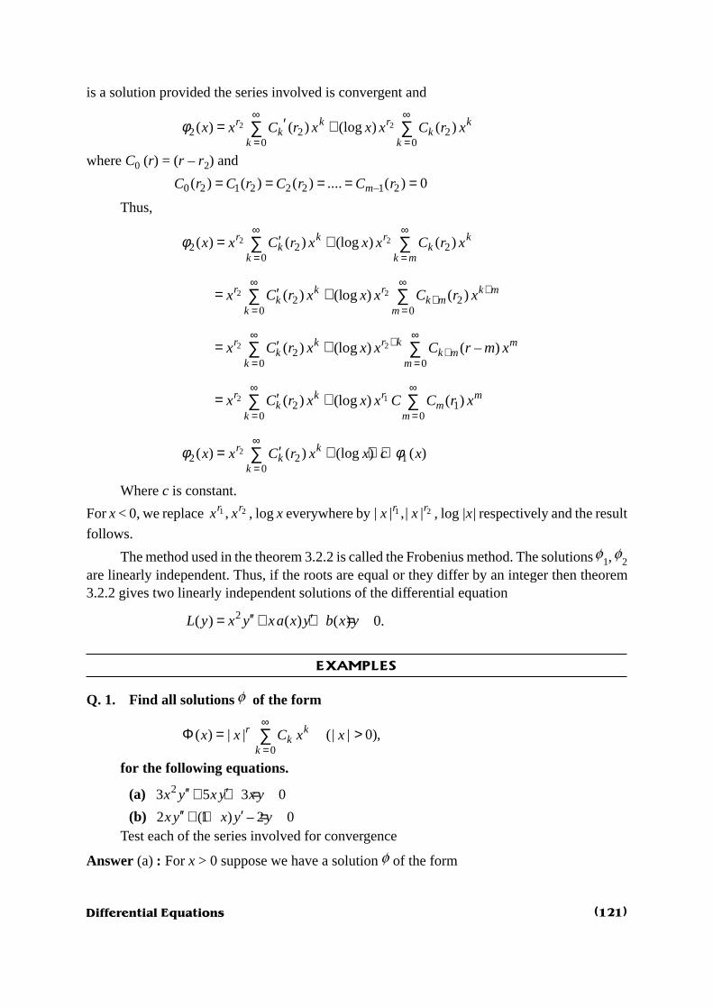
Differential Equations
is a solution provided the series involved is convergent and
2 2
2 2 20 0
( ) ( ) (log ) ( )∞ ∞
= =′= +∑ ∑r rk k
k kk k
x x C r x x x C r xφ
where C0 (r) = (r – r2) and
0 2 1 2 2 2 –1 2( ) ( ) ( ) .... ( ) 0= = = = =mC r C r C r C r
Thus,
2 2
2 2 20
( ) ( ) (log ) ( )r rk kk k
k k mx x C r x x x C r xφ
∞ ∞
= =′= +∑ ∑
2 2
2 20 0
( ) (log ) ( )r rk k mk k m
k mx C r x x x C r x
∞ ∞+
+= =
′= +∑ ∑
2 2
20 0
( ) (log ) ( – )∞ ∞+
+= =
′= +∑ ∑r r kk mk k m
k mx C r x x x C r m x
2 1
2 10 0
( ) (log ) ( )∞ ∞
= =′= +∑ ∑r rk mk m
k mx C r x x x C C r x
2
2 2 10
( ) ( ) (log ) ( )∞
=′= + ⋅ ⋅∑r kk
kx x C r x x c xφ φ
Where c is constant.
For x < 0, we replace 1 2,r rx x , log x everywhere by 1 2| | ,| |r rx x , log |x| respectively and the result
follows.
The method used in the theorem 3.2.2 is called the Frobenius method. The solutions f1, f2
are linearly independent. Thus, if the roots are equal or they differ by an integer then theorem3.2.2 gives two linearly independent solutions of the differential equation
2( ) ( ) ( ) 0.L y x y xa x y b x y′′ ′= + + =
EXAMPLES
Q. 1. Find all solutions f of the form
0
( ) | | (| | 0),r kk
kx x C x x
∞
=Φ = >∑
for the following equations.
(a) 23 5 3 0x y x y x y′′ ′+ + =(b) 2 (1 ) – 2 0xy x y y′′ ′+ + =
Test each of the series involved for convergence
Answer (a) : For x > 0 suppose we have a solution f of the form
(121)

Differential Equations
00
( ) , 0∞
== ≠∑r k
kk
x x c x cφ
then –1
0( ) ( )
∞
=′ = +∑r k
kk
x x k r c xφ and –2
0( ) ( ) ( –1)
∞
=′′ = + +∑r k
kk
x x k r k r c xφ
Let 2( ) 3 5 3′′ ′= + +L y x y xy xy therefore
[ ] 1
0 0( ) ( ) 3( ) ( –1) 5( ) 3r k r k
k kk k
L x x k r k r k r c x x c xφ∞ ∞ +
= == + + + + + ⋅∑ ∑
[ ] [ ]{ } 10 1 03 ( –1) 5 3( 1) 5( 1) 3r rr r r c x r r r c c x += + + + + + +
[ ]{ } 22 13( 2) ( 1) 5( 2) 3 ...rr r r c c x ++ + + + + + +
Let ( ) 3 ( –1) 5 (3 2)q r r r r r r= + = + then
[ ] [ ]1 20 1 0 2 1( ) ( , ) ( ) ( 1) 3 ( 2) 3 ....r r rL x r q r c x q r c c x q r c c xφ + += + + + + + + +
[ ]0 –11
( ) ( ) 3r r kk k
kq r c x q r k c c x
∞+
== + + +∑
( ) ( , ) 0L x rφ = only if q(r) = 0 and
–1( ) 3 0k kq r k c c+ + = for k = 1, 2, 3,.....
The indicial equation q (r) = 0 implies r (3r + 2) = 0 that is 2
0, – .3
r = Let r1 = 0, 22
–3
r = .
(By choice r1 > r2)
Since ( ) (3 2), ( ) ( ) (3( ) 2) ( ) (3 3 2)q r r r q r k r k r k r k r k= + + = + + + = + + +
–1( ) 3 0+ + =k kq r k c c gives
–1–3
, 1,2,3...( )
= =+k
kc
c kq r k
0(–3)
( ) ( –1) ( – 2)..... ( 1)
k c
q r k q r k q r k q r=
+ + + +
Case 1 : r1 = 0
For c0 = 1 we obtain 0(–3)
( ) ( –1)..... (1)=
k
kc
cq k q k q
(–3)
(3 2)( –1)(3 –1)( – 2) (3 – 4).....1 5
k
k k k k k k=
+ ⋅
(–3)
! 5 8 11 (3 – 4)(3 –1)(3 2)
k
k k k k=
⋅ ⋅ ⋅ ⋅⋅⋅ +Thus,
11
(–3)( ) 1
! 5 8 11 (3 – 4) (3 –1) (3 2)
k k
k
xx
k k k kφ
∞
== +
⋅ ⋅ ⋅ ⋅⋅ ⋅ +∑
(122)

Differential Equations
Case 2 : 22
–3
=r
For c0 = 1 we obtain 0(–3)2 5 7 1
– – – .....3 3 3 3
=
k
kc
cq k q k q k q
Since q(r) = r (3r + 2)
0(–3)
2 5 8 1– (3 ) – (3 – 3) – (3 – 6) ..... 3
3 3 3 3
= ⋅
k
kc
ck k k k k k
0(–3)
!1 4 7 (3 – 8)(3 – 5)(3 – 2)
k c
k k k k=
⋅ ⋅ ⋅ ⋅⋅Thus,
2–
32
1
(–3)( ) 1
! 1 4 7 (3 – 8) (3 – 5) (3 – 2)φ
∞
=
= + ⋅ ⋅ ⋅⋅⋅ ⋅
∑k k
k
xx x
k k k k
To obtain solutions for x < 0, we replace xr by |x |r. Thus,
11
(–3)( ) 1
! 5 8 11 (3 – 4)(3 –1)(3 2)
k k
k
xx
k k k kφ
∞
== +
⋅ ⋅ ⋅ ⋅⋅ ⋅ +∑
and
2–
32
(–3)( ) | | 1
! 1 4 7 (3 – 8) (3 – 5) (3 – 2)
k kxx x
k k k kφ
= + ⋅ ⋅ ⋅ ⋅⋅ ⋅
∑
These functions f1 and f2 will be solutions for x ¹ 0, provided both the series convergeson some interval containing x = 0.
Let 10
( ) ( )kk
x d xφ∞
== ∑
Using ratio test we obtain
1( ) (–3) 3 | |
0( ) ( 1) (3 5) ( 1) (3 5)
k
k
d x x xd x k k k k
+ = = →+ + + +
as k ® ¥ provided |x | < ¥. Thus, series defining f1 is convergent for all finite x.
Let 21
( ) ( )kk
x d xφ∞
== ∑
Using ratio test we obtain
1( ) –3 3 | |0
1( ) (3 1) ( 1)3 ( 1)3
k
k
d x x xd x k kk k
+ = = →+ + + +
as k ® ¥ provided |x | < ¥. Thus, series defining f2 is convergent for all finite x.
Thus f1, f2 are solutions of the given equation.
(123)

Differential Equations
(b) Suppose for x > 0 we have a solution f of the form
00
( ) , 0r kk
kx x C x cφ
∞
== ≠∑
Let ( ) 2 (1 ) – 2 0L y xy x y y′′ ′= + + = then
–1 –1
0 0( ) ( , ) 2( ) ( –1) ( )φ
∞ ∞+ +
= == + + + +∑ ∑k r k r
k kk k
L x r k r k r C x k r C x
0 0( ) – 2k r k r
k kk k
k r C x C x∞ ∞
+ +
= =+ +∑ ∑
[ ] –1
0 02( ) ( –1) ( ) ( – 2)k r k r
k kk k
k r k r k r C x k r C x∞ ∞+ +
= == + + + + + +∑ ∑
[ ] [ ]{ }–10 1 02 ( –1) 2( 1) ( ) ( 1) ( – 2)= + + + + + +r rr r r c x r r r c r c x
[ ]{ } 12 12( 2) ( 1) ( 2) ( –1) rr r r c r c x ++ + + + + + +⋅⋅⋅ ⋅
[ ]–10 –1
1( ) ( ) ( – 3)
∞ +
== + + + +∑r k r
k kk
q r c x q r k C r k C x
The indicial equation q(r) = 0 implies 2r2 – 2r + r = 0, r (2r – 1) = 0 gives 1
0,2
r =
Let 1 21
and 0.2
r r= =
Observe that r1 ¹ r2 and r1 – r2 is not a positive integer. L(f ) (x, r) = 0 if and only ifq(r) = 0 and
–1( ) ( – 3) 0+ + + =k kq r k C r k C or
–1( – 3)
– for 1,2,3( )
kk
r k CC k
q r k
+= =+
Since ( ) (2 –1)q r r r= therefore ( ) ( ) (2 2 –1)+ = + +q r k r k r k and
0( – 3) ( – 4) ( – 5) ( – 2)
– – – .......... –( ) ( –1) ( – 2) ( 1)
+ + += + + + + + k
r k r k r k rC C
q r k q r k q r k q r
0(–1) ( – 3) ( – 4) ( – 5) ( – 2)
( ) (2 2 –1) ( –1) (2 2 – 3).....( 1)(2 1)
k r k r k r k r C
r k r k r k r k r r
+ + + ⋅⋅⋅=+ + + + + +
Case 1 : 1 01
, 12
= =r C
5 7 9 3(–1) – – – –
2 2 2 21 1 3 3
(2 ) – (2 – 2) – (2 – 4) (2)2 2 2 2
⋅⋅ ⋅⋅ = + ⋅⋅ ⋅⋅
k
k
k k kC
k k k k k k
(–1) (2 – 5) (2 – 7) (2 – 9) 3 (–1)(–3)
2 !(2 1) (2 –1) (2 – 3) (3)
⋅⋅ ⋅⋅=+ ⋅⋅⋅⋅
k
k
k k k
k k k k
(124)

Differential Equations
(–1) (3)
2 !(2 1) (2 –1) (2 – 3)
k
k k k k k=
+and
1
21
1
3(–1)( ) 1 .
2 !(2 1) (2 –1) (2 – 3)
k k
kk
xx x
k k k kφ
∞
=
= + =
+ ∑
Case 2 : r2 = 0, C0 = 1
(–1) ( – 3) ( – 4) ( – 5) (–1)(–2)
(2 –1)( –1) (2 – 3) (1)
k
kk k k
Ck k k k
⋅⋅ ⋅⋅=⋅⋅ ⋅⋅
for k = 3, C3 = 0 therefore Ck = 0 for k = 1, 2, 3,...
0
1(–2)
– 2(1)
= =CC
12
(–1) 2 1– .
2 3 6 3= = =
⋅C
C
and 22 0 1 2( )x c c x c xφ = + +
21
1 23
x x= + +
Thus, for x ¹ 0 we get two solutions
1
21
1
3(–1)( ) | | 1
2 !(2 1) (2 –1)(2 – 3)
k k
kk
xx x
k k k kφ
∞
=
= +
+ ∑
2
2( ) 1 23
φ = + + xx x
Check that series in the first solution is convergent Let 10
( ) ( ).∞
== ∑ k
kx d xφ
Using ratio test
1 | |0
2( 1) (2 3) 2( 1) (2 3)k
k
d x xd k k k k
+ = = →+ + + +
as k ® ¥ if | x | < ¥. The series convergent for finite x.
Q. 2. Obtain two linearly independent solutions of the following equations which arevalid near x = 0.
(a) 2 3 (1 ) 0x y xy x y′′ ′+ + + =
(b) 2 22 – 2 0x y x y y′′ ′+ =Ans. :
(a): For x > 0 suppose we have a solution f of the form
(125)

Differential Equations
00
( ) , 0∞
== ≠∑r k
kk
x x C x Cφ
Let 2( ) 3 (1 )L y x y xy x y′′ ′= + + +
( ) ( , ) ( ) ( –1) 3 ( ) += + + + + +∑ ∑ ∑r k r k k rk k kL x r x k r k r C x x k r C x C xφ 1r k
kx C x ++ ∑
[ ] 1
0 0( )( –1) 3( ) 1)
∞ ∞+ + +
= == + + + + + +∑ ∑k r k r
k kk k
k r k r k r C x c x
( ) ( , ) 0=L x rφ implies
[ ] 1
0 0( )( –1) 3( ) 1 0k r k r
k kk k
k r k r k r C x C x∞ ∞
+ + +
= =+ + + + + + =∑ ∑
[ ] [ ]{ } 10 1 0( –1) 3 1 ( 1)( ) 3( 1) 1 ++ + + + + + + +r rr r r C x r r r C C x
[ ]{ } 22 1( 2) ( 1) 3( 2) 1 0++ + + + + + + +⋅⋅⋅ =rr r r C C x
( ) ( –1) 3 1 0q r r r r= + + = is indicial equation.
2 2( ) – 3 1 ( 1)q r r r r r= + + = +
[ ] [ ]1 20 1 0 2 1( ) ( ) ( ) ( 1) ( 2) 0+ += + + + + + + + ⋅⋅⋅ =r r rL x q r C x q r C C x q r C C qφ
[ ]0 –11
( ) ( )∞ +
== + + +∑r r k
k kk
q r C x q r k C C x = 0
( ) ( ) 0L xφ = if and only if q(r) = 0 and
–1( ) 0+ + =k kq r k C C for k = 1, 2, 3,...
q(r) = 0 implies (r + 1)2 = 0 that is r = – 1 is a repeated root. Here r = r1 = r2 = – 1.
–1( ) 0+ + =k kq r k C C for k = 1, 2, 3,...
Since, 2 2( ) ( 1) , ( ) ( 1)q r r q r k r k= + + = + + and
–1
2
–
( 1)=
+ +k
kC
Cr k
2 2 2 2 2–1 –1 –1 –1 –1
( 1) ( ) ( –1) ( – 2) ( 2)r k r k r k r k r
= ⋅⋅⋅ + + + + + +
[ ]0
2
(–1)
( 2) ( 3) ( – 2) ( –1)( ) ( 1)=
+ + ⋅⋅ ⋅ + + + + +
kC
r r r k r k r k r k
The first solution will be constructed by substituting Ck’s at r = – 1 in the series. Ck atr = – 1 is
02
(–1)
!=
k
kC
Ck
(126)

Differential Equations
10
( )∞
== ∑r k
kk
x x C xφ
–1
20
(–1)
!
∞
== ∑
kk
kx x
kThe series converges for all finite x.
Since r = – 1 is the root of multiplicity 2, i.e. r = r1 = r2 = – 1, the second solution
1
2 1 10
( ) ( ) (log ) ( )r kk
kx x C r x x xφ φ
∞
=′= +∑
[ ]0
2
(–1).
( 2) ( 3)( 4) ( 1)=
+ + + ⋅⋅⋅ + +
k
kC
Cr r r r k
Define D = (r + 2) (r + 3) (r + 4) ..... (r + k + 1) then
'
0 2
(–2) 1 1 1 1(–1)
2 3 4 1 = + + + ⋅⋅⋅ + + + + + +
kkC C
r r r r kD
2
(–2) (–1) 1 1 1 1(–1)
1 2 3!
k
kCkk
′ = + + + ⋅⋅⋅ +
–1
2 120
(–2) (–1) 1 1 1( ) 1 (log ) ( )
2 3!
kk
kx x x x x
kkφ φ
∞
=
= + + + ⋅⋅⋅ + + ∑
To obtain solution for x < 0 we replace x by |x |.
Thus, the two solutions are
–1
1 20
(–1)( ) | |
!
k k
k
xx x
kφ
∞
== ∑
–1
2 20
(–2) (–1) 1 1 1( ) | | 1
2 3!
kk
kx x x
kkφ
∞
=
= + + + ⋅⋅⋅ + ∑
–12
0
(–1)(log | |) | | .
!
k k
k
xx x
k
∞
=+ ∑
Check that series in both the solutions converge.
(b): For x > 0 suppose we have a solution f of the form
00
( ) ( 0)∞
== ≠∑r k
kk
x x C x Cφ
Let 2 2( ) 2 – 2L y x y x y y′′ ′= + then
1
0( ) ( , ) ( ) ( –1) 2( ) – 2
∞ + + + +
= = + + + + ∑ k r k r k r
k k kk
L x r k r k r C x k r C x C xφ
[ ] 1
0 0( ) ( –1) – 2 2( )
∞ ∞+ + +
= == + + + +∑ ∑k r k r
k kk k
k r k r C x k r C x
(127)

Differential Equations
[ ] [ ]{ } 10 1 0( –1) – 2 ( 1)( ) – 2 2 += + + +r rr r C x r r C r C x
[ ]{ } 22 1( 2) ( 1) – 2 2( 1) ++ + + + + +⋅⋅⋅rr r C r C x
[ ]0 –11
( ) ( ) 2( –1)∞
+
== + + + +∑r r k
k kk
q r C x q r k C r k C x
Indicial equation is ( ) ( –1) – 2 0q r r r= = gives 2 – – 2 ( – 2)( 1) 0r r r r= + = r = – 1, 2.
1 22, –1r r= = and 1 2– 3r r = a positive integer.
If r1 – r2 is a positive integer, we try a series using the smallest root. If c0 and c3 both turnout to be arbitrary, we obtain the general solution by this method. Otherwise the general solutionwill involve a logarithm as it did in the case of equal roots. That logarithmic case is treated intheorem 3.2.2.
Let us consider the series solution as –1
20
( ) ( smallest root = –1)∞
== −∑ k
kk
x c x rφ
–1 –1
0( ) ( –1) ( – 2) 2 ( –1) – 2φ
∞
== +∑ ∑ ∑k k k
k k kk
L k k c x k c x c x
[ ] –1
0 0( –1)( – 2) – 2 2 ( –1)k k
k kk k
k k c x k c x∞ ∞
= == +∑ ∑
[ ]{ }–1 –10 –1
1(2 – 2) ( –1) ( – 2) – 2 2( – 2)
∞
== + +∑ k
k kk
c x k k c k c x
Since f is a solution L(f ) = 0 i.e.
0.c0 = 0 i.e. c0 is arbitary.
[ ] –1( –1)( – 2) – 2 2( – 2) 0 1,2,3,...k kk k c k c k+ = =
1 0 1 0
2 2
3 2 3 3
1 – 2 – 2 0 i.e. –
2 – 2 0 i.e. 0
3 (2 – 2) 2 0 i.e. 0 0 is arbitary.
k c c c c
k c c
k c c c c
= = =
= = =
= + = ⋅ = ⇒
[ ] –1( –1)( – 2) – 2 2( – 2) 0 4,5,6,...k kk k c k c k+ = =
2–1( – 3 ) 2( – 2) 0k kk k c k c+ =
–1( – 3) 2( – 2) 0k kk k c k c+ =
–12( – 2)
– , 4,5,6,7,....( – 3)
= =kk
k cc k
k k
3–2( – 2) –2( – 3) –2( – 4) –2(2)
( – 3) ( –1) ( – 4) ( – 2) ( – 5) 4 1
= ⋅⋅ ⋅ ⋅ k
k k kc c
k k k k k k
–3
3(–2) ( – 2)( – 3) ( – 4) (2)
( – 3)( –1) ( – 4)( – 2) ( – 5) 4 1
k k k kc
k k k k k k
⋅⋅⋅=⋅⋅⋅ ⋅
(128)

Differential Equations
–3
3(–2) ( – 2)6
!
k kc
k=
Thus, we get a solution
–3
–1 0 1 2 –10 0 3 3
4
(–2) ( – 2)6( ) – 0
!φ
∞
== + ⋅ + + ∑
kk
k
kx c x c x x c x c x
k
–3–1 2 –1
0 34
(–2) ( – 2)6( –1)
!
kk
k
kc x c x x
k
∞
=
= + +
∑
–1 2 20 3
1
(–2) ( 1)6(1– )
( 3)!
kk
k
kc x x c x x
k
∞+
=
+= + + +
∑
–1 20 3
1
(–2) ( 1)6(1– ) 1
( 3)!
kk
k
kc x x c x x
k
∞
=
+= + + +
∑
Thus, we get two solutions
–1 21 2
1
(–2) ( 1)6( ) (1– ) and ( ) 1
( 3)!
kk
k
kx x x x x x
kφ φ
∞
=
+= = + +
∑
These are two solutions for x > 0 for x < 0 replace x by |x | we get,
–1 21 2
1
(–2) ( 1)6( ) | | (1– ) and ( ) | | 1
( 3)!
kk
k
kx x x x x x
kφ φ
∞
=
+= = + +
∑
Check that series appearing in f2 is convergent series.
EXERCISE
1. Compute indicial polynomials and their roots for the following equations.
(a) 2 2( ) – 0x y x x y y′′ ′+ + =
(b) 2 2 1– 0
4x y x y x y ′′ ′+ + =
(c) 2 4 24 (4 – 5 ) ( 2) 0x y x x y x y′′ ′+ + + =
(d) 2 2( – 3 ) 0xx y x x y e y′′ ′+ + =
2. Find a solutions f of the form
0( ) , ( 0)r k
kk
x x C x xφ∞
== >∑
for the following equations.
(129)

Differential Equations
(a) 2 22 ( – ) 0x y x x y y′′ ′+ + =
(b) 2 2( – ) 0x y x x y y′′ ′+ + =3. For each equation obtain two linearly independent solutions valid near origin
(a) 2 ( –1) 3( –1) – 0x x y x y y′′ ′+ =
(b) 2 5(1 2 ) 5 0xy x y y′′ ′+ + + =
(c) 3 (2 – ) – 2 0′′ ′+ =xy x y y
(d) 22 (1– 2 ) – 4 0xy x y xy′′ ′+ =
4. Consider the following equation near x = 0
(a) 2 2 22 (5 ) ( – 2) 0x y x x y x y′′ ′+ + + =
(b) 24 – 4 3(cos ) 0xx y xe y x y′′ ′ + =Compute the roots r1, r2 of the indicial equation for each relative to x = 0.
5. Obtain two linearly independent solutions of the following equations which are validnear x = 0.
(a) 2 – 2 ( 1) 2( 1) 0x y x x y x y′′ ′+ + + =
(b) 2 2– 2 (4 – 2) 0x y x y x y′′ ′ + =
(c) – (4 ) 2 0x y x y y′′ ′+ + =
(d) 2 2 ( – 2) 2(2 – 3 ) 0x y x x y x y′′ ′+ + = .
Answers :
1. (a) 21 2( ) –1 ; 1, –1= = =q r r r r
(b)2
1 21 1 1
( ) – ; , –4 2 2
= = =q r r r r
(c)2
1 29 1 1
( ) – ; 2,4 2 4
= + = =q r r r r r
(d) 21 2( ) 1 ; , –= + = =q r r r i r i
2. (a)1 1
2 2–
21 2
0 0
(–1) (–1)( ) , ( )
1 3 5 7 (2 1) 2 !
∞ ∞
= == ∑ = ∑ =
⋅ ⋅ ⋅ ⋅⋅⋅ ⋅ +
k k k k x
kk k
x xy x x y x x x e
k k
(b)–
1 20 0
(1 ) ( –1 ) (– )(1– ) ( –1– )( ) ; ( )
(1 2 )(2 2 ) ( 2 ) ! ! (1 2 )(2 – 2 ) ( – 2 )
∞ ∞
= =
+ ⋅⋅⋅⋅ + ⋅⋅⋅⋅= ∑ = ∑+ + ⋅⋅⋅⋅ + + ⋅⋅⋅⋅
i k i K
k k
i i k i i i k iy x x x y x x x
i i k i k k i i k i
(130)

Differential Equations
3. (a)1 12 2
1 2211– ; –
4 –1
∞ −
== ∑ =
n
n
xy y x x
n
(b)1
2
3– –2
1 23(–5)
1 ; –10!(2 1) (2 3)
= + ∑ =+ +
nxy y x x
n n n
(c)13
1 20 1
(3 4) ( 1); 1
2 5 8 (3 – 1)4 3 !
+∞ ∞
= =
+ += ∑ = + ∑⋅ ⋅ ⋅ ⋅ ⋅ ⋅⋅
n n
nn n
n x n xy y
nn
(d)2 1 2
1 20 1
2; 1
3 7 11 (4 –1)2 !
k k k
kn n
x xy y
kk
+∞ ∞
= == ∑ = + ∑
⋅ ⋅ ⋅⋅⋅ ⋅
4. (a) 1 21
; –22
r r= =
(b) 1 23 1
;2 2
r r= =
5. (a) 21 2( ) ; ( ) ( –1)xy x x y x x e= =
(b)2 –1 2 2
1 24
2( ) ; ( ) 1 3 6 –3 4 log| |
( –3) !
∞
=
= = + + ∑ −
k k
k
xy x x y x x x x x x
k k
(c)2 5
1 26
601 11 ;
2 12 ( – 5)! ( –1)( – 2)
∞
== + + = + ∑
n
n
xy x x y x
n n n n
(d)–3 1
2 3 41 2
4
6(–2)– 2 2 ;
!
n n
n
xy x x x y x
n
+∞
== + = + ∑
Unit 3 : The Bessel equation
If a is a constant, Re a ³ 0 the Bessel equation of order a is the equation
2 2 2( – ) 0x y xy x yα′′ ′+ + =This has the form
2 2
21 –
0x
y y yx x
α′′ ′+ + =
where 1
( )p xx
= and 2 2
2–
( ) . 0= =xq x x
x
α is a singular point. Since the denominator of p(x)
does not contain x to a power higher than one and the denominator of q(x) (i.e. x2) does notcontain the factor x to a power higher then 2, x = 0 is a regular singular point. Therefore thepower series solution f will have the form
(131)

Differential Equations
0
( ) r kk
kx x C xφ
∞
== ∑
Let 2 2 2( ) ( – ) .L y x y xy x yα′′ ′= + +
2 2( ) ( , ) ( ) ( –1) ( ) ( – )k r k r k r
k k kL x r k r k r C x k r C x x C xφ α+ + += + + + + +∑ ∑ ∑
2 2
0 0( )( –1) ( ) – k r k r
k kk k
k r k r k r C x C xα∞ ∞
+ + +
= = = + + + + + ∑ ∑
2 2 1
0 1( –1) – ( 1) ( 1) –r rr r r C x r r r C xα α + = + + + + +
{ }2 2–2
2( ) –α
∞ +
= + + + ∑ k r
k kk
k r C C x
The indicial equation is2( ) ( –1) – 0q r r r r α= + =
2 2( ) – 0.q r r α= =The indicial polynomial q(r) has two roots r1 = a and r2 = –a . We shall construct solutions
for x > 0. We consider three cases namely a = 0, 2a is not a positive integer and 2a is a positiveinteger.
Case 1 : a = 0
Since the roots are both equal to zero by theorem 3.2.2, there are two solutions f1, f2 ofthe form
1 1 2 2 1( ) ( ) and ( ) ( ) (log ) ( ),φ σ φ σ φ= = +x x x x x x x
Where s1(x), s2(x) have power series expansions which converge for all finite x.Since a = 0,
2 2( )L y x y x y x y′′ ′= + +
Suppose 1 00 0
( ) ( 0)k kk k
k kx x C x C x Cασ
∞ ∞
= == = ≠∑ ∑ be a solution of L(y) = 0. Then
2
12 1 0
( ) ( ) ( –1)σ∞ ∞ ∞ +
= = == + +∑ ∑ ∑k k k
k k kk k k
L x k k C x k C x C x
1 –22 2 2
( –1) k k kk k k
k k kk k C x C x k C x C x
∞ ∞ ∞
= = == + + +∑ ∑ ∑
[ ]{ }1 –22
( –1) kk k
kC x k k k C C x
∞
== + + +∑
Since s1 is a solution L (s1) = 0 for all x. Therefore C1 = 0 and [ ] –2( –1) 0,k kk k k C C+ + =k = 2, 3, 4
Thus, C1 = 0 and
(132)

Differential Equations
2–2– for 2,3,4,.....k kk C C k= =
The recurrance relation becomes
–22
– , 2,3,4,.....kk
CC k
k= =
Since 1 3 5 7 2 10, ..... .... 0.nC C C C C += = = = = = =
The choice C0 = 1 implies
2
0 22 42 2 2 2 2 2 2
(–1)1 1 1– – , – – – ,.......
2 2 4 4 2 2 4
C CC C
= = = = = ⋅ In general
2 2 2 2 2 2 2(–1) (–1)
, 1,2,3,.....2 4 6 (2 ) 2 !
= = =⋅ ⋅ ⋅⋅⋅ ⋅
m m
m mC m
m mThus s1 contains only even powers of x and we get
2
1 2 20
(–1)( )
2 !
m m
mm
xx
mσ
∞
== ∑
The function defined by this series is called the Bessel function of zero order of the firstkind and is denoted by J0. Thus
2
0 2 20
(–1)( )
2 !
m m
mm
xJ x
m
∞
== ∑
Let 00
( ) ( )kk
J x d x∞
== ∑
Using ratio test
2 21
2 2 20
2 ( 1) 4( 1)k
k
d x xd k k
+ = = →+ +
as k ® ¥ if | x | < ¥. Thus, the series converges for |x | < ¥ and J0 (x) is the first solution ofBessel equation with a = 0.
Now we determine a second solution f2 for the Bessel equation of order zero (i.e. a = 0).
Let 1 0( ) ( )x J xφ = then the solution f2 has the form
2 2 1( ) ( ) (log ) ( )x x x x xφ σ φ= +
1 00
(log ) ( ), ( 0).kk
kc x x x Cφ
∞
== + =∑
Since f2 is second solution
2 22 2 2 2( ) ( ) 0L x x x xφ φ φ φ′′ ′= + + =
–1 1
2 11
( )( ) (log ) ( )k
kk
xx k c x x x
x
φφ φ∞
=′ ′= + +∑
(133)

Differential Equations
–2 1 12 12
2
2 ( )( ) ( –1) – (log )k
kk
xx k k c x x
x x
φ φφ φ∞
=
′′′ ′′= + +∑
2 1 12
( ) ( ) ( –1) 2 ( ) – ( )kk
kL x k k c x x x xφ φ φ
∞
=′= +∑
21 1 1
1(log ) ( ) (log ) ( )φ φ φ
∞
=′′ ′+ + + +∑ k
kk
x x k c x x x x x
2 21
0(log ) ( )k
kk
x c x x x xφ∞
=+ +∑
21
2 1 0( –1) 2 ( )k k k
k k kk k k
k k c x k c x c x x xφ∞ ∞ ∞
+
= = =′= + + +∑ ∑ ∑
2 21 1 1(log )( )x x x xφ φ φ′′ ′+ + +
Since 21 1 1 1( ) 0,L x xφ φ φ φ′′ ′= + + =
2 1 –2 12 2 2
( )( ) ( –1) 2 ( )φ φ∞ ∞ ∞
= = =′= + + + +∑ ∑ ∑k k k
k k kk k k
L x k k c x c x k c x c x x x
Since L(f2 ) should be zero and 1 0( ) ( ),x J xφ ′ ′=2 –1
1 0 2 2(–1) 2
( ) ( ) ,2 ( !)
φ ′ ′= = ∑m m
mm x
x J xm
Thus2
1 –2 2 22 2 2
(–1) 2( –1) –2
2 ( !)
m mk k k
k k k mk k k
m xk k c x c x k c x c x
m
∞ ∞ ∞
= = =+ + + =∑ ∑ ∑ ∑
[ ]{ }2
1 –2 2 22
(–1) 2( –1) –2
2 ( !)
m mk
k k mk
m xc x k k k c c x
m
∞
=+ + + =∑ ∑
Since the series on right has only even powers of x, all odd terms on the left hand sideshould be zero c1 = c3 = c5 = c7 = .... = c2n+1 = .....= 0.
The relation for the other coefficients that is for k even (let k = 2m) is
[ ] 2 2 –2 2 2(–1) 2
2 (2 –1) 2 –22 ( !)
+ + =m
m m mm
m m m c cm
12
2 2 –2 2 –2 2(–1)
[4 ] , 1,2,3,4,.....2 ( !)
m
m m mm
m c c mm
++ = =
1
2 2 –22 2 –2 2
(–1)1– , 1,2,3,4....
(2 ) 2 ( !)
m
m mm
mc c m
m m
+ = =
c0 = 0
(134)

Differential Equations
2 42 2 2 2 2 21 1 1 1 1 1
, – – – 122 4 2.2 2 2 4
c c = = = +
6 2 2 2 2 2 2 2 21 1 1 1 1 1 1
1 12 3 26 2 4 3 2 4 2 4 6
c = + + = + + +
and it can be shown by induction that
2 2 2
(–1) 1 1 1 1 11 , 1,2,3,....
–1 – 2 3 22 ( !) = + + + ⋅⋅⋅ + + + =
m
m mc m
m m mm
The solution thus determined is called a Bessel function of zero order of second kind, andis denoted by K0. Hence,
2
0 021
(–1) 1 1 1( ) – 1 (log ) ( )
2 3 2( !)
mm
m
xK x x J x
mm
∞
=
= + + + ⋅⋅ ⋅+ + ∑
Using the ratio test we can check that the series on the right is convergent for all finitevalues of x.
Now we compute solution for Bessel equation of order a, where a ¹ 0 and Re a ³ 0.
2 2 2( ) ( – ) 0L y x y x y x yα′′ ′= + + =Let x > 0. The roots of indicial equation are
r1 = a, r2 = – a.
Let us find out the solution corresponding to r1 = a. A solution f1 (x) has the form
1 00
( ) , ( 0)kk
kx x c x cαφ
∞
== ≠∑
Then
10 0
( )( ) ( )( –1) ( )k kk k
k kL x k k c x k c xα αφ α α α
∞ ∞+ +
= == + + + +∑ ∑
2 2
0 0–α αα
∞ ∞+ + +
= =+ ∑ ∑k k
k kk k
c x c x
2 2
0 0( ) ( –1) ( ) – k k
k kk k
k k k c x c xα αα α α α∞ ∞+ + +
= = = + + + + + ∑ ∑
2 2 2
0 0( ) – k k
k kk k
k c x c xα αα α∞ ∞+ + +
= = = + + ∑ ∑
2 2 1 2 2
0 12
0 ( 1) – ( ) – kk
kc x c x k c xα α αα α α α
∞+ +
= = ⋅ + + + + ∑
–22
kk
kc x α∞ +
=+ ∑
(135)

Differential Equations
( )2 2 1 2 20 1 –2
20 ( 1) – ( ) –α α αα α α α
∞+ +
=
= ⋅ + + + + + ∑ kk k
kc x c x k c c x
Thus, 1( ) ( ) 0L xφ = implies
0 00 0,c c⋅ = is arbitrary.
c1 = 0,
2 2–2( ) – 0 2, 3,4,.....k kk c c kα α + + = =
Since 2 2( ) – (2 ) 0 for 2,3,......,k k k kα α α+ = + ≠ =
–2(2 ) 0k kk k c cα + + = gives
–2– .
(2 )k
kc
ck kα
=+
Since 1 2 10, 0 for 0,1,2, 3,.....kc c k+= = =
that is all odd terms are zero.
We find
0 0
2 2
––
2(2 2) 2 ( 1)α α= =
+ +c c
c
02
4 2–
4(2 4) 2 ( 1) ( 2)α α α= =
+ + +cc
c
04 4 4
6 6
–– – –
6(2 6) 12( 3) 2 3!( 3) 2 3!( 1)( 2) ( 3)
cc c cc
α α α α α α= = = =
+ + ⋅ + ⋅ + + +
6 0
8 8
– –
8(2 8) 2 4!( 1) ( 2) ( 3)( 4)α α α α α= =
+ + + + +c c
c
In general,
02 2
(–1).
2 !( 1)( 2) ( 3) ( )
m
m m
cc
m mα α α α=
+ + + ⋅⋅⋅ +Thus the solution f1 becomes
1 00
( ) ( 0)kk
kx x c x cαφ
∞
== ≠∑
2
0 21
(–1)
2 !( 1)( 2) ( )
m m
mm
xc x x
m m
α α
α α α
∞
== +
+ + ⋅⋅ ⋅ +∑
for a = 0 and c0 = 1, f1(x) becomes J0 (x). Before going for the second solution let us definegamma function and study some properties of gamma function.
(136)

Differential Equations
Definition 3.3.1
The gamma function is defined by
– –1
0
( ) , (Re 0)x zz e x dx z∞
Γ = >∫
Lemma 1 : ( 1) ( )z z zΓ + = Γ
Proof : –
0
( 1) x zz e x dx∞
Γ + = ∫
–
0
Lim x zT e x dx
∞
→∞= ∫
–
– –1
0 0
| – ––1
Tx TLim z x zT
x
ex e ze dx→∞
=
= ⋅
∫
– –1
0→∞= ∫
TLim x zT z e x dx
– –1
0
∞= ∫ x zz e x dx
( )z z= Γ
Observe that – –
0| – 0 0T
Lim z x Lim z TT Tx e T e→∞ →∞= ⋅ =
By definition 3.3.1
–
0
(1) 1xe dx∞
Γ = =∫
Thus, if z is a positive integer n,
( 1) ( ) ( –1)( – 2)n n n n n nΓ + = Γ =
( ) ( –1) ( – 2) ( – 3) (1)n n n n= ⋅⋅⋅ ⋅Γ = n !
Thus, gamma function is an extension of the factorial function to numbers which are notintegers.
Suppose Re z < 0 and z is not a negative integer then there is a natural number N such that
– N < Re z < – N + 1
But then Re (z + N) > 0 and therefore we can define
( ) ( –1)( – 2) ( 1) ( ).z N z N z N z z zΓ + = + + ⋅⋅⋅ ⋅ + Γ Then
( )
( ) , (Re 0)( –1) ( – 2) ( – 3) ( 1)
z Nz z
z N z N z N z z
Γ +Γ = <+ + + ⋅⋅ ⋅⋅ +
The gamma function is not defined at 0, –1, –2, –3,.......
We have a solution f1 (x) as
(137)
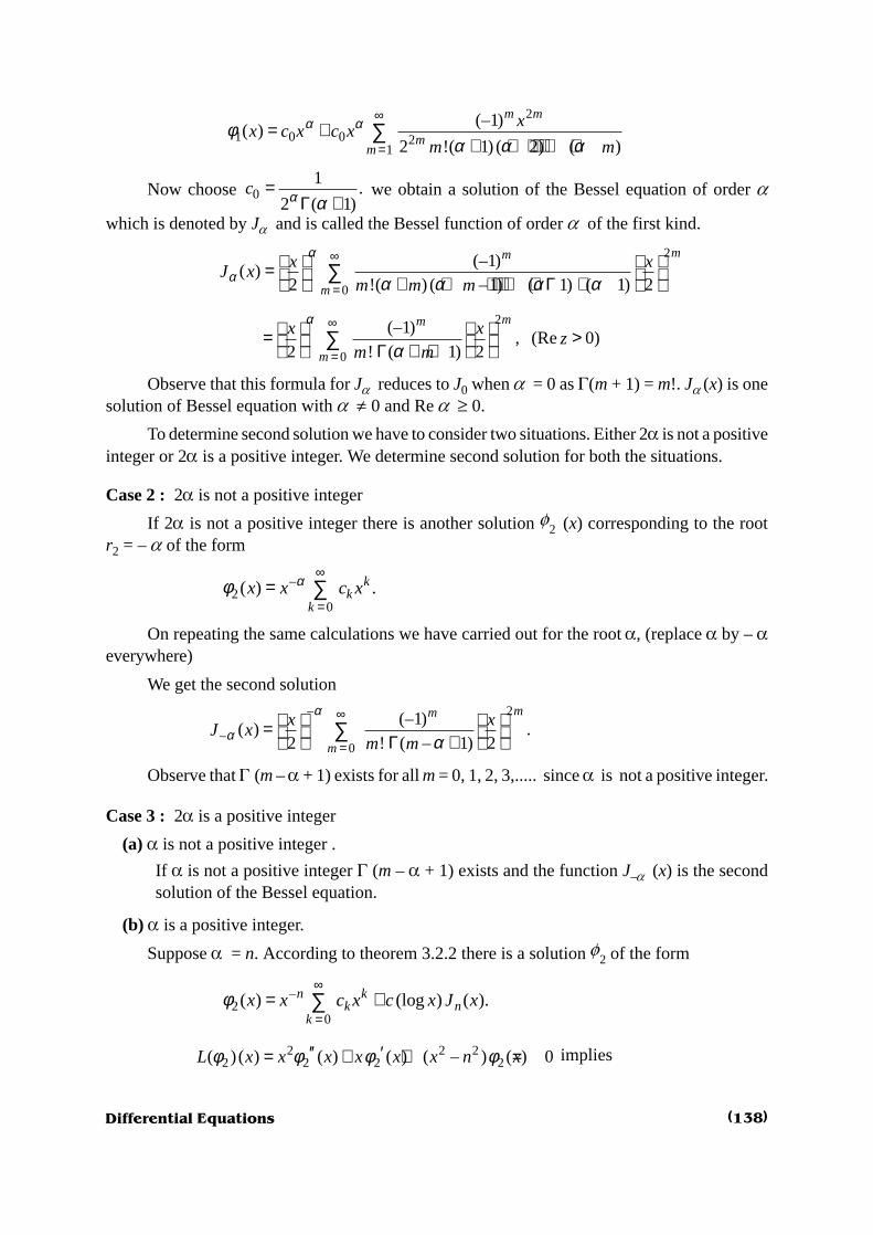
Differential Equations
2
1 0 0 21
(–1)( )
2 !( 1) ( 2) ( )
m m
mm
xx c x c x
m m
α αφα α α
∞
== +
+ + ⋅⋅ ⋅⋅ +∑
Now choose 01
.2 ( 1)
c α α=
Γ + we obtain a solution of the Bessel equation of order a
which is denoted by Ja and is called the Bessel function of order a of the first kind.
2
0
(–1)( )
2 !( ) ( –1) ( 1) ( 1) 2
mm
m
x xJ x
m m m
α
α α α α α
∞
=
= + + ⋅⋅ ⋅⋅ + Γ + ∑
2
0
(–1), (Re 0)
2 ! ( 1) 2
mm
m
x xz
m m
α
α
∞
=
= > Γ + + ∑
Observe that this formula for Ja reduces to J0 when a = 0 as G(m + 1) = m!. Ja (x) is onesolution of Bessel equation with a ¹ 0 and Re a ³ 0.
To determine second solution we have to consider two situations. Either 2a is not a positiveinteger or 2a is a positive integer. We determine second solution for both the situations.
Case 2 : 2a is not a positive integer
If 2a is not a positive integer there is another solution f2 (x) corresponding to the rootr2 = – a of the form
–
20
( ) .kk
kx x c xαφ
∞
== ∑
On repeating the same calculations we have carried out for the root a, (replace a by –aeverywhere)
We get the second solution
– 2
–0
(–1)( ) .
2 ! ( – 1) 2
α
α α
∞
=
= Γ + ∑
mm
m
x xJ x
m m
Observe that G (m – a + 1) exists for all m = 0, 1, 2, 3,..... since a is not a positive integer.
Case 3 : 2a is a positive integer
(a) a is not a positive integer .
If a is not a positive integer G (m – a + 1) exists and the function J–a (x) is the secondsolution of the Bessel equation.
(b) a is a positive integer.
Suppose a = n. According to theorem 3.2.2 there is a solution f2 of the form
–
20
( ) (log ) ( ).n kk n
kx x c x c x J xφ
∞
== +∑
2 2 22 2 2 2( ) ( ) ( ) ( ) ( – ) ( ) 0L x x x x x x n xφ φ φ φ′′ ′= + + = implies
(138)

Differential Equations
2 – –2
20
2( – ) ( – –1) – ( log )k n
k n n nk
c cx k n k n c x J J c x J
x x
∞
=
′ ′′+ +
∑
– –1
0( – ) ( log )k n
k n nk
cx k n c x J c x J
x
∞
=
′+ + +
∑
2 2 –
0( – ) ( log ) ( ) 0.
∞
=
+ + =
∑ k n
k nk
x n c x c x J x
Since Jn (x) is the first solution corresponding to a = n, 2 2 2( – )n nx J x J x n′′ ′+ + ( ) 0,nJ x =and above equation gets reduce to
– –
0 0( – )( – –1) 2 – ( – )k n k n
k n n k nk k
k n k n c x c x J c J k n c x c J∞ ∞
= =′+ + +∑ ∑
– 2 2 –
0 0– 0k n k n
k kk k
c x n c x∞ ∞+
= =+ =∑ ∑
Therefore
2 – – 2
0 0( – ) ( – –1) ( – ) – 2 ( ) 0.k n k n
k k nk k
k n k n k n n c x c x c x J x∞ ∞ +
= = ′+ + + = ∑ ∑
or 2 2 – – 2
0 0( – ) – 2 ( ) 0k n k n
k k nk k
k n n c x c x c x J x∞ ∞
+
= = ′+ + = ∑ ∑
that is – 2 2 1– 2 2 – – 20
2 00 (1– ) – ( – ) –n n k n k n
k kk k
c x n n c x k n n c x c x∞ ∞ +
= = ⋅ + + + ∑ ∑
2 ( ) 0.nc x J x′+ =
Since – 2 – 2 1– 2 2– 2 3– 20 1 2 3
0
k n n n n nk
kc x c x c x c x c x
∞ + + + + +
== + + + + ⋅⋅ ⋅⋅∑
––2
2,k n
kk
c x∞
== ∑ we get
{ }– 2 2 1– 2 2 –0 1 –2
20 (1– ) – ( – ) – 0.n n k n
k k nk
c x n n c x k n n c c x c x J∞
= ′⋅ + + + + = ∑
On multiplying by xn we have
[ ]0 1 –22
0 (1– 2 ) ( – 2 )∞
=⋅ + + +∑ k
k kk
c n c x k k n c c x –2 ( ) nnc x J x x′= ⋅ .............. (3.3.1)
Since the first solution is Ja (x) with a = n and for a = n, G (m + a + 1) = G (m + n + 1)= (m + n) ! we have
2
0
(–1)( )
! ( )! 2
m nm
nm
xJ x
m m n
+∞
=
= + ∑
(139)

Differential Equations
Therefore
2 –1(2 ) (–1) 1
( )! ( )! 2 2
m nm
nm n x
J xm m n
++ ′ = + ∑
Thus equation (3.3.1) becomes
[ ]2 2
0 1 –2 2 –12 0
(2 )(–1)0 (1– 2 ) ( – 2 ) –
! ( )! 2
m m nk
n k m nk m
m n xc n c x k k n c c x c
m m n
+∞ ∞
+= =
+⋅ + + + =+
∑ ∑
.............. (3.3.2)
The series on the right side begin with x2n and since n is positive integer, the right side donot contain any odd terms. Therefore c1 = 0 c2k+1 = 0 for k = 1, 2, 3,.... and if n > 1 then
–2( – 2 ) 0, for 2,3,4,...., 2 –1.k kk k n c c k n+ = =
Since 1 3 5 7 2 –10, .... 0.nc c c c c= = = = = =
Whereas –2
(2 – )k
kc
ck n k
+= gives
0 02
2 42 4,
4 2( – 2)2 ( –1) 2 2 ( – 2) ( –1)
c ccc c
nn n n= = =
⋅ ⋅ ⋅
04
6 66 2( – 3) 3!2 ( – 3) ( – 2) ( –1)
ccc
n n n n= =
⋅
in general 02 2
, 1,2,3,....., –12 !( –1) ( – 2)( – 3) ( – )
j j
cc j n
j n n n n j= =
⋅⋅ ⋅⋅ ...(3.3.3)
In particular
0
2 –2 2 –22 ( –1)!( –1)!n n
cc
n n=
On comparing the coefficients of x2n in equation (3.3.2) we get
2 –2 –1 –1– –
!2 ( –1)!2n n n
n cc c
n n= =
Thus 02 –2 2 –2 2 –1
–2 ( –1)! 2 ( –1)!
n n n
c cc
n n= =
and therefore 0–1
– .2 ( –1)!n
cc
n= .....( 3.3.4 )
Since c2 n–2 is used to find c, c2n remains undetermined, but the remaining coefficientsc2n+2, c2n + 4, c2n + 6,..... can be obtained by comparing the coefficients of x2(n + j) in equation(3.3.2).
2 2 2 2 –2 2 –1
(–1) (2 ) 1(2 2 )(2 2 – 2 ) – 1,2,3.....
!( )! 2+ + +
++ + + = =+
j
n j n j j nj n
n j n j n c c c jj n j
(140)

Differential Equations
2 2 2 2 –2 2 –1
(–1) (2 ) 14 ( ) – 1,2,3.....
!( )! 2+ + +
++ + = =+
j
n j n j j nj n
j n j c c c jj n j
for j = 1 we have
2 2 2 1
(–1) ( 2)4( 1) –
( 1)! 2n n n
nn c c c
n+ +
++ + =+
2
2 2 11
1 –1 4( 1)4 2 ( 1)!
nn n
ccc
n nn+ +
= + + + ⋅ ⋅ +
Choose 21– 1 1 1 1
14( 1) 2 3 44 2 ( 1)!+
= + + + + ⋅⋅⋅ ⋅+ + ⋅ ⋅ +n
n
c cn nn
i.e. 2 1– 1 1 1 1
12 3 42 !+
= + + + + ⋅⋅ ⋅⋅ + n nc
cnn
Then 2 2 11 1 1 1 1
1 12 3 4 14 2 ( 1)!
+ ++ = + + + + + ⋅⋅⋅⋅ + + + ⋅ +n n
cc
n nnfor j = 2 we have
2
2 4 2 23(–1) ( 4)
4 2( 2) – –2!( 2)!2
n nnc n
n c cn
+ +++⋅ + =
+
2 4 3– 2 1
1 –2 4 2( 2)4 2 2!( 2)! 2
+ + = + + ⋅ + ⋅ ⋅ +n n
cc
n nn 1
1 1 11 1
2 3 14 2 ( 1)!nc
nn+ + + + + ⋅⋅⋅⋅ + + ⋅ +
2 2– 1 1 1 1 1 1
1 12 2 2 3 14 ( 2)! 2 +
= + + + + + + ⋅⋅ ⋅⋅ + + + + + nc
n n nn
2 2– 1 1 1 1 1
1 12 2 3 14 ( 2)! 2n
cn nn +
= + + + + + ⋅⋅ ⋅⋅ + + + +
2
4– (–1) 1 1 1 1 1
1 12 2 3 12 2!( 2)! 2 +
= + + + + + ⋅⋅⋅⋅ + + + ⋅ + nc
n nn
It can be shown by induction that
2 2 2
– (–1) 1 1 1 1 1 11 1 ,
2 3 2 32 !( )! 2+ +
= + + + ⋅⋅⋅ ⋅ + + + + + ⋅⋅⋅ ⋅ + + ⋅ +
m
n m n m
cc
m n mm n m
1,2,3,....m=
Finally we get a solution f2
–2
0( ) ( log ) ( )n k
k nk
x x c x c x J xφ∞
== +∑
2 –1
– – 2 1 – 2 –2 –1 2
0 2 –1( log ) ( )
∞−
= == + + + +∑ ∑
nn k n n n n n k
k n n k nk k n
x c x x c x x c x x c x c x J x
Since all odd terms c2k+1 = 0, k = 1, 2, 3,....., we get,
(141)

Differential Equations
2–1– – 0
2 0 2 11
1 1 1( ) – 1
2 32 !( –1)( – 2) ( – ) 2 !
jnn n n
j nj
x c cx x c x x
nj n n n j nφ +
=
= + + + + ⋅⋅⋅ ⋅+ ⋅⋅ ⋅⋅∑
2
21
(–1) 1 1 1 1 1 1– 1 1
2 3 2 32 !( )! 2
+∞
+=
+ + + ⋅⋅ ⋅⋅ + + + + + ⋅⋅⋅ ⋅+ + ⋅ + ∑
m m n
n mm
c x
m n mm n m
( log ) ( ).nc x J x+
Where c0 and c are constants related by equation (3.3.4) when c = 1, the resulting solutionf2 is often denoted by Kn. If c = 1 then c0 = – 2n–1 (n – 1) ! and
–1 2–1– –1 –
2 21
(–1) 2 ( –1)!( ) – 2 ( –1)!
2 !( –1)( – 2) ( – )
n jnn n n
jj
n xx x n x
j n n n jφ
== +
⋅⋅ ⋅⋅∑
11 1 1
– 12 32 !
n
nx
nn+ + + + ⋅⋅ ⋅⋅ +
2–1
1
(–1)–
2 !( )! 2
n mmn
m
xm n m
+
=
⋅ +
∑
1 1 1 1 1 11 1
2 3 2 3m n m
+ + + ⋅⋅ ⋅⋅ + + + + + ⋅⋅ ⋅⋅ + + ( log ) ( )nc x J x+
– – 2–1
1
– ( – –1)!1 1– ( –1)!
2 2 2 2 ! 2
n n jn
j
n jx x xn
j=
= + ⋅ ∑
11 1 1
– 12 32 !+
+ + + ⋅⋅⋅⋅ +
n
nx
nn
2
1
(–1)–
2 ! ( )! 2
n mm
m
xm n m
+∞
=
⋅ +
∑
1 1 1 1 1 1
1 1 ( log ) .2 3 2 3 nc x J
m n m
+ + + ⋅⋅ ⋅⋅ + + + + + ⋅⋅ ⋅⋅ + + + The function f2 when c = 1 is denoted by Kn . Thus
– 2–1
0
( – –1)!1 1 1 1 1 1( ) – – 1
2 2 ! 2 2 ! 2 3 2=
= ⋅ + + + ⋅⋅ ⋅⋅ + ∑
n j nn
nj
n jx x xK x
j n n
2
1
(–1)1 1 1 1 1 1 1– 1 1
2 2 !( )! 2 2 3 2 3
∞
=
+ + + ⋅⋅⋅⋅ + + + + + ⋅⋅ ⋅⋅ + + + ∑
n mm
m
x xm n m m m n
+ (log ) ( ).nx J x .......... (3.3.5)
The function Kn is called a Bessel function of order n of second kind.
In this section we have derived all kinds of Bessel functions. We list all these functionshere.
(1) Bessel function of zero order of the first kind denoted by J0(x) and defined by
2
0 2 20
(–1)( )
2 !
m m
mm
xJ x
m
∞
== ∑
(2) Bessel function of zero order of second kind denoted by K0(x) is
2
0 021
(–1) 1 1 1( ) – 1 (log ) ( )
2 3 2!
mm
m
xK x x J x
mm
∞
=
= + + + ⋅⋅ ⋅⋅ + + ∑
(142)

Differential Equations
(3) Bessel function of order a of first kind denoted by Ja (x) is defined by
2
0
(–1)( ) , (Re 0)
2 ! ( 1) 2
mm
m
x xJ x
m m
α
α αα
∞
=
= > Γ + + ∑
(4) Bessel function of order n of second kind is defined by equation (3.3.5)
J0(x) is a solution of Bessel equation with a = 0 K0(x) is a second solution of Besselequation with a = 0 obtained according to theorem 3.2.2 where the roots of indicial equationr1 = r2 = a = 0. Ja (x) is the first solution of Bessel equation where 2a is not a positive integerand Kn(x) is the second solution of Bessel equation where a = n a positive integer.
Depending upon the situation choose a and then find the required Bessel function.
EXAMPLES
Ex. 1. Suppose f is any solution of 2 2 0x y xy x y′′ ′+ + = for x > 0 and let 12( ) ( )ψ φ=x x x .
show that y satisfies the equation 2 2 1( ) 0
4x y x y′′ + + = for x > 0.
Ans. : Since f is a solution, 2 2 0x x xφ φ φ′′ ′+ + =
Let 1 1 1
–2 2 21
( ) ( ) then ( )2
x x x x x xψ φ ψ φ φ′ ′= = +
and 3 1 1
– –2 2 21
( ) –4
ψ φ φ φ′′ ′ ′′= + +x x x x
1 3 5
2 2 2 21( ) –
4x x x x xψ φ φ φ′′ ′ ′′= + +
1 1
22 21– ( )
4x x x xφ φ φ′ ′′= + +
1 1
2 2 22 21– (– ) (Since 0)
4x x x x x xφ φ φ φ φ′′ ′= + + + =
1
2 221 1– ( ) – ( ) ( )
4 4x x x xφ ψ= + = +
Thus, 2 2 1( ) ( ) ( ) 0
4x x x xψ ψ′′ + + =
and y satisfies the equation 2 2 1( ) 0
4x y x y′′ + + = for x > 0.
Ex. 2. Let f be a real valued non-trivial solution of ( ) 0y x yα′′ + = on a < x < b
Let y be a real valued non-trivial solution of ( ) 0y x yβ′′ + = on a < x < b
Here a, b are real valued continuous functions.
(143)

Differential Equations
Suppose that ( ) ( ),x xβ α> (a < x < b) Show that if x1 and x2 are successive zeros of f ona < x < b, then y must vanish at sone point r1, x1 < r1 < x2.
Ans. : Suppose ( ) 0xψ ≠ for 1 2x x x< < then either ( ) 0xψ > 1 2( , )x x x∀ ∈ or ( ) 0xψ <
1 2( , )x x x∀ ∈ suppose ( ) 0xψ > for 1 2x x x< < .
Since x1 and x2 are successive zeros either 1 2 1 2( ) 0 on ( , ) or ( ) 0 on ( , )x x x x x xφ φ> <suppose 1 2( ) 0 on ( , )x x xφ > . Then
( – ) – – ( )xψ φ φψ ψ φ φψ α ψ φ βψ φ′ ′ ′ ′′ ′′= = + ( – )β α φψ=
[Since f is solution of 0, ( ) 0α φ α φ′′ ′′+ = + =y y x similarly ( ) ( ) 0x xψ β ψ′′ + = ]
Thus, ( – ) ( – ) 0 ( , , 0)ψ φ φψ β α φψ β α φ ψ′ ′ ′ = > > > Integration of above inequality
between x1 and x2 gives
[ ] [ ]2 2 2 2 1 1 1 1( ) ( ) – ( ) ( ) – ( ) ( ) – ( ) ( ) 0x x x x x x x xψ φ φ ψ ψ φ φ ψ′ ′ ′ ′ >
But x1 and x2 are zeros of f therefore 1 2( ) ( ) 0x xφ φ= = and above inequality becomes
2 2 1 1( ) ( ) – ( ) ( ) 0.ψ φ ψ φ′ ′ >x x x x
Since ( ) 0xφ > for 1 2 1 1and ( ) 0, ( – ) 0x x x x x hφ φ< < = < for h > 0. Therefore
1 11 0
( ) – ( – )( ) 0
φ φφ →′ = >Limh
x x hx
h
Similarly 2( ) 0xφ′ <
Let 2 1 1 2 1 2( ) – and ( ) then , 0,x L x L L Lφ φ′ ′= = > 2 1 1 2– ( ) – ( ) 0x L x Lψ ψ >
i.e. 1 2 2 1( ) ( ) 0L x L xψ ψ+ <
But 1 2 1 2( ) 0 for and , 0.x x x x L Lψ > < < >
This is a contradiction to our assumption that ( ) 0xψ > for 1 2.x x x< < Therefore y takes
both positive and negative values in the interval (x1, x2) and hence ∃ there exists 1 1 2( , )r x x∈such that 1( ) 0.rψ =
Ex. 3. Show that J0 has an infinity of positive zeros.
Ans. : J0 (x) is a solution of differential equation 2 2 0x y x y x y′′ ′+ + =
If 12
0( ) ( )x x J xψ = then by example 1, y satisfies
21
1 0, ( 0)4
y y xx
′′ + + = > The function satisfies ( ) sinf x x= satisfies 0y y′′ + =
Since 21
1 14x
+ > and sin x = 0 has infinitely many zeroes , 0,1,2,3,....x n nπ= =
(144)

Differential Equations
By above example 2
1( ) 1 and ( ) 1
4x x
xβ α = + =
12
0( ) ( )x x J xψ = has a zero between np and (n + 1)p for n = 0, 1, 2,..... Thus, J0 (x) has
infinite number of positive zeros.
Ex. 4. (a) If 12
00 and ( ) ( )x x J xλλ φ λ> = shows that 22
1– .
4xλ λ λφ φ λ φ′′ + =
(b) If l, m are positive constants, show that
12 2
0
( – ) ( ) ( ) (1) (1)λ µ λ µλ µ φ φ φ φ ′=∫ x x d x – (1) (1).µ λφ φ ′
(c) If 0 0and ( ) 0, ( ) 0,J Jλ µ λ µ≠ = = show that
1 1
00 0
( ) ( ) ( )x x d x x J xλ µφ φ λ=∫ ∫ 0( ) 0J x dxµ =
Ans. (a) : J0 (x) is solution of 2 2 0x y xy x y′′ ′+ + = therefore J0 (l x) is solution of
2 2 2 2 0x y x y x yλ λ λ+ + =&& & where ‘.’ represents differentiation with respect to l x.
If 1 1 1
–2 2 2
0 0 01
( ) ( ) then ( ) ( ) ( )2λ λφ λ φ λ λ λ′ ′= = + ⋅x x J x x x J x x J x
3 1 1
– – 22 2 20 0 0
1( ) – ( ) ( ) ( )
4λφ λ λ λ λ λ′′ ′ ′′= + +x x J x x J x x J x
1 1
2 2 22 20 0 0
1( ) – ( ) ( ) ( )
4λφ λ λ λ λ λ ′′ ′′ ′′= + + x x x J x x x J x xJ x
1 1
2 22 20 0
1– ( ) – ( )
4x J x x x J xλ λ λ = +
12 22
01
– ( )4
x J x xλ λ = +
Therefore 2 2 21( ) ( ) 0.
4x x x xλ λφ λ φ ′′ + + =
22
1( ) ( ) –
4x x
xλ λ λφ φ λ φ′′ + =
Ans. (b) : 22
1( ) ( ) –
4x x
xµ µ µφ φ µ φ′′ + =
22
1( ) ( ) –
4x x
xλ λ λφ φ λ φ′′ + = .
(145)

Differential Equations
Multiply first equation by fl and second equation by fm and subtract these equations.
2 2 2 2– – ( – ) .µ λ λ µ µ λ µ λ λ µφ φ φ φ µ φ φ λ φ φ λ µ φ φ′′ ′′ = + =
Thus, ( )2 2( – ) –λ µ µ λ λ µλ µ φ φ φ φ φ φ ′′ ′=
Integrate above equation between 0 to 1. Since
1 1
2 20 0( ) ( ), (0) 0 and ( ) ( ), (0) 0.x x J x x x J xλ λ µ µφ λ φ φ µ φ= = = =
Therefore
12 2
0
( – ) ( ) ( ) (1) (1) – (1) (1)x x d xλ µ µ λ λ µλ µ φ φ φ φ φ φ′ ′=∫
Ans. (c) :1
2 2
0
( – ) ( ) ( ) (1) (1) – (1) (1)x x d xλ µ µ λ λ µλ µ φ φ φ φ φ φ′ ′=∫
Since, 0 0( ) 0, (1) 0 and ( ) 0 (1) 0.λ µλ φ µ φ= = = ⇒ =J J
\1
2 2
0
( – ) ( ) ( ) 0x x d xλ µλ µ φ φ =∫
i.e.
1 11 12 2
0 00 0
( ) ( ) ( ) ( ) 0x x dx x J x x J x d xλ µφ φ λ µ= =∫ ∫
i.e.1
0 00
( ) ( ) 0.x J x J x dxλ µ =∫
Ex. 5. Show that J0¢ (x) = – J1 (x).
Ans. : 2
0 20
(–1)( )
2!
∞
=
= ∑
mm
m
xJ x
m
2 –1
0 2 21
2(–1)( )
! 2
∞
=′ = ∑
mm
mm
m xJ x
m
2 –1
2 2 –11
(–1)
! 2
∞
== ∑
mm
mm
m x
m
2 11
2 2 10
( 1)(–1)
( 1)! 2
++∞
+=
+=+
∑mm
mm
m x
m(Replace m by m + 1)
2
0
(–1)–
2 !( 1)! 2
∞
=
= + ∑
mm
m
x xm m
1– ( )J x=
(146)

Differential Equations
Ex. 6. Define, 1
( )k when k is a non-positive integer to be zero. Show that if n is a positive
integer the formula for J–n(x) gives.
– ( ) (–1) ( )nn nJ x J x=
Ans. : – 2
–0
(–1)( )
2 2! ( – 1)
∞
=
= +∑
n mm
nm
x xJ x
m m n
– 2(–1) 1(As 0 for 0)
2 ! ( – )! 2 ( )
∞
=
= = ≤ ∑
n mm
m n
x xk
m m n k
– 2 2
0
(–1)(Replace by )
2 ( )! ! 2
n m mm n
m
x xm m n
m n m
++∞
=
= + + ∑
2
0
(–1)(–1)
2 ! ( – )! 2
n mmn
m
x xm m n
∞
=
= ∑
(–1) ( ).nnJ x=
Ex. 7. Show that
(a) –1( ) ( ) ( )x J x x J xα αα α′ =
(b) – –1( ) ( ) – ( )x J x x J xα α
α α+′ =
Ans. (a) : 2
0
(–1)( )
2 2! ( 1)
α
α α
∞
=
= + +∑
mm
m
x xJ x
m m
\ 22
0
(–1)( )
2! ( 1)2
αα
α α α
∞
=
= + +∑
mm
m
x xx J x
m m
2 2
20
(–1)1
! ( 1)2 2
α
α α
+∞
==
+ +∑
m m
mm
x
m m
2 2 –1
20
(–1) (2 2 )1( )
! ( 1)2 2
αα
α αα
α
+∞
=
+′ =+ +
∑m m
mm
m xx J
m m
–1 2
0
(–1)2 2! ( )
αα
α
∞
=
= +∑
mm
m
x xx
m m
–1( )x J xαα=
Ans. (b) : 2(–1)
( )2 2! ( 1)
α
α α = + +
∑mmx x
J xm m
(147)

Differential Equations
2
–
0
(–1)12! ( 1)2
αα α α
∞
=
= + +∑
mm
m
xx J
m m
( )2 –1
–2
1
2(–1)1
! ( 1)2 2α
α α α
∞
=
′ =+ +
∑mm
mm
m xx J
m m
1 2 1
2 20
(–1) 2( 1)1
( 1)! ( 2)2 2α α
+ +∞
+=
+=+ + +
∑m m
mm
m x
m m
2
10
(–1)–
! ( 2)2 2α α
∞
+=
=+ +
∑m m
mm
x x
m m
But 1 2
10
(–1)( )
2 2! ( 2)
α
α α
+ ∞+
=
= + +∑
mm
m
x xJ x
m m
\
2–
1 10
(–1)– –
2! ( 2)2α
α α α
∞+ +
=
= + +∑
mm
m
x xx J
m m
Thus ( )– –1–x J x Jα α
α α+′ =
8. Show that
(a) –1 1( ) – ( ) 2 ( )J x J x J xα α α+ ′=
(b) –1–1 1( ) ( ) 2 ( )J x J x x J xα α αα++ =
Ans. –1–1( ) ( )x J x x J x J x Jα α α α
α α α αα′ ′= = + .......... (i)
– – – –1 –1– ( ) ( ) –x J x x J x J x Jα α α α
α α α αα+ ′ ′= = + .......... (ii)
(a) Multiply equation (i) by x–a and equation (ii) by xa and add.
–1 –1–1 1( ) – ( ) ( – ) 2 ( )α α α α α αα α+ ′ ′ ′= + + =J x J x x x J J J J x
Thus, –1 1( ) – ( ) 2 ( )α α α+ ′=J x J x J x
(b) Multiply equation (i) by x–a and equation (ii) by xa and subtract.
–1–1 1( ) ( ) 2 ( )J x J x x J xα α αα++ =
Thus, using results of example 7 we have proved the required result.
Ex. 9. Show that 0 1( ) – ( )′ =K x K x
Ans. : 2
0 021
(–1) 1 1 1( ) – 1 log ( )
2 3 2!
∞
=
= + + + ⋅⋅⋅⋅ + + ∑
mm
m
xK x x J x
mm
(148)

Differential Equations
2 –1
0 0 02 21
2(–1) 1 1 1 1( ) – 1 ( ) log ( )
2 3! 2
∞
=
′ ′= + + + ⋅⋅⋅ ⋅ + + + ∑
mm
mm
m xK x J x x J x
m xm
22 –1
02 2 –1 21 0
(–1) (–1)1 1 1 1– 1 log
2 3 2! 2 !
mmm m
mm m
m x xx J
m xm m
∞ ∞
= =
′= + + + ⋅⋅ ⋅⋅ + + + ∑ ∑
22 –1 2 –1
2 2 –1 2 22 2
(–1) (–1)1 1 1 1– 1 1–
2 2 3 4! 2 ! 2
mm m m
m mm m
m xx x xm xm m
∞ ∞
= =
= + + + ⋅⋅ ⋅⋅ + + + ∑ ∑
0log ( )x J x′+
2 –1
02 2 –12
(–1)1 1 1 1 1– 1 log ( )
4 2 2 3! 2
m m
mm
x xm x J x
x mm
∞
=
′= + + + + + ⋅⋅⋅ ⋅+ + ∑
2 –2
02 2 –22
(–1)1 1 1 1 1– – 1 log
4 2 2 2 3 –1! 2
m m
mm
xx xm x J
x mm
∞
=
′= + + + + + ⋅⋅⋅⋅ + + ∑
Replace m by m + 1 and use the result 0 1–J J′ = then
21
01
(–1) ( 1)1 1 1 1 1( ) – – 1
4 2 ( 1)! ! 2 2( 1) ( 1) 2 3
mm
m
mx x xK x
x m m m m m
+∞
=
+ ′ = + + + + + ⋅⋅⋅⋅ + + + + ∑
1– log ( )x J x⋅
2(–1)1 1 1 1 1 1
2 14 2 2 !( 1)! 2 1 2 3
mmx x xx m m m m
= + + + + + + ⋅⋅⋅ ⋅+ + + ∑
1– log ( )x J x⋅
1– ( )= K x
Thus, 0 1( ) – ( )′ =K x K x
EXAMPLES
1. Let f be any solution for x > 0 of the Bessel equation of order a2 2 2( – ) 0x y xy x yα′′ ′+ + =
Put
12( ) ( ).x x xψ φ= show that y satisfies equation
2
2
1–
41 0y yx
α ′′ + + =
2. Show that if a > 0 then Ja has an infinite number of positive zeros.
3. Show that J0¢ satisfies the Bessel equation of order one
(149)
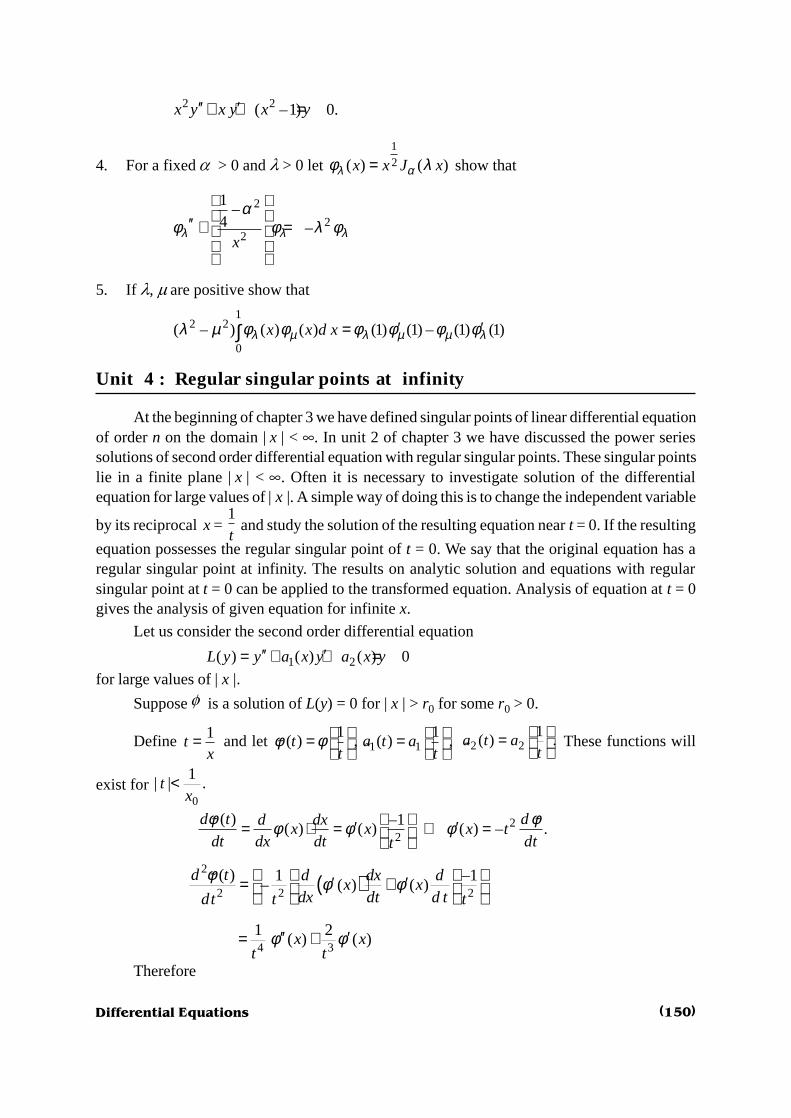
Differential Equations
2 2( –1) 0.x y x y x y′′ ′+ + =
4. For a fixed a > 0 and l > 0 let 12( ) ( )x x J xλ αφ λ= show that
2
22
1–
4 –x
λ λ λ
αφ φ λ φ
′′ + =
5. If l, m are positive show that
12 2
0
( – ) ( ) ( ) (1) (1) – (1) (1)x x d xλ µ λ µ µ λλ µ φ φ φ φ φ φ′ ′=∫
Unit 4 : Regular singular points at infinity
At the beginning of chapter 3 we have defined singular points of linear differential equationof order n on the domain |x | < ¥. In unit 2 of chapter 3 we have discussed the power seriessolutions of second order differential equation with regular singular points. These singular pointslie in a finite plane |x | < ¥. Often it is necessary to investigate solution of the differentialequation for large values of |x |. A simple way of doing this is to change the independent variable
by its reciprocal x = 1t and study the solution of the resulting equation near t = 0. If the resulting
equation possesses the regular singular point of t = 0. We say that the original equation has aregular singular point at infinity. The results on analytic solution and equations with regularsingular point at t = 0 can be applied to the transformed equation. Analysis of equation at t = 0gives the analysis of given equation for infinite x.
Let us consider the second order differential equation
1 2( ) ( ) ( ) 0′′ ′= + + =L y y a x y a x y
for large values of |x |.
Suppose f is a solution of L(y) = 0 for |x | > r0 for some r0 > 0.
Define 1t
x= and let 1 1
1 1( ) , ( ) ,t a t a
t tφ φ = = % % 2 2
1( ) .a t a
t =
% These functions will
exist for 0
1| | .<t
x
2
2
( ) –1( ) ( ) ( ) – .
d t dd dxx x x t
dt dx dt dtt
φ φφ φ φ ′ ′= ⋅ = ⇒ =
% %
( )2
2 2 2( ) 1 –1
– ( ) ( )d t d dx d
x xdx dt d tdt t t
φ φ φ ′ ′= +
%
4 31 2
( ) ( )x xt t
φ φ′′ ′= +
Therefore
(150)

Differential Equations
2
42( )
( ) – 2 ( )d t
x t t xdt
φφ φ′′ ′=%
2
4 22
– 2 –dd
t t td tdt
φφ =
%%
and
4 3 21 2( ) ( ) ( ) 2 ( ) ( ) (– ) ( ) ( ) ( )φ φ φ φ φ φ′′ ′ ′= = + + +% % % % %% % %L L t t t t a t t t a t t
4 3 2
1 2( ) 2 – ( ) ( ) ( ) ( )t t t a t t t a t tφ φ φ ′′ ′= + + % % %% %
( ) 0L φ = gives ( ) 0.L φ =%% Thus, φ% satisfies
4 3 2
1 2( ) 2 – ( ) ( ) 0L y t y t a t t y a t y ′′ ′= + + = % % % .......(3.4.1)
Where the prime denotes differentiation with respect to t.
Convertsely if φ% satisfies ( ) 0L y =% the function f will satisfy L(y) = 0. The equation
(3.4.1) is called the induce equation associated with L(y) = 0 and the substitution 1
.xt
=
Definition 3.4.1 :
We say that infinity is a regular singular point for 1( ) ( ) ( ) ( )L y y x a x y x′′ ′= +
2( ) ( ) 0a x y x+ = if t = 0 is a regular singular point of
4 3 2
1 2( ) ( ) 2 – ( ) ( ) ( ) ( ) 0L y t y t t t a t y t a t y t ′′ ′= + + = % % %
( )L y% is equivalent to the equation
1 22 4
2 – ( ) ( )( ) ( ) ( ) 0
t a t a ty t y t y t
t t′′ ′+ + =
% %
On comparing this equation with the equation in definition 3.1.3(b) we see that
1 22 4
2 – ( ) ( )( ) and ( )
t a t a tp t q t
t t= =
% %
If 10
( ) kk
ka t t tα
∞
== ∑% and 2
20
( ) β∞
== ∑%
kk
ka t t t where the series converge for 0
0
1| | , 0,t r
r< >
then the denomiantor of p(t) will not contain a factor t to a power higher than one and thedenominator of q(t) will not contain a factor t to a power higher than two. By definition
3.1.3(b) t = 0 is a regular singular point of ( ) 0=%L y and therefore infinity is a regular singularpoint of L(y) = 0.
EXAMPLES
Ex. 1. Check whether infinity is regular singular point of 2 0,x y a x y b y′′ ′+ + = where a, bare constants.
Ans. : Put1
.xt
=
(151)

Differential Equations
2( ) – ( )′ = ⋅ = &d y d t
y x t y td t d x
where .dot (.) represents differentiation with respect to t.
[ ] [ ] 2 2( ) ( ) ( ) – ( ) – 2 ( ) (– )d d td
y x y x y x t y t t y t td x d t d x
′′ ′= = = && &
4 3( ) 2 ( )t y t t y t= +&& &
2 4 3 221 1
( ) ( ) 2 ( ) – ( ) ′′ ′+ + = + + ⋅ + && & &x y x axy by t y t t y t a t y t bytt
[ ]2 ( ) 2 – ( )t y t a t y t b y= + +&& &
[ ]( ) 0L y x = implies
22 –
( ) ( ) ( ) 0.+ + =&&a b
y t y t y tt t
This equation is of form 0.y p y q y′′ ′+ + = Since denomination of p contains a factor
, 1rt r >/ and denominator of q contain a factor , 2, 0rt r t> =/ is a regular singular point. Thus,
infinity is a regular singular point of the given differential equation.
Ex. 2. Show that infinity is not a regular singular point for the equation
0y a y b y′′ ′+ + =where a, b are constants, not both zero.
Ans. : 2( ) – ( )y x t y t′ = &
4 3( ) ( ) 2 ( )y x t y t t y t′′ = +&& &
and ( ) ( ) ( ) 0′′ ′+ + =y x a y x by x gives
4 3 2( ) 2 ( ) – ( ) ( ) 0.t y t t y t a t y t b y t+ + =&& & &
Therefore
2 42 –
( ) ( ) ( ) 0t a b
y t y t y tt t
+ + =&& &
Here 2 42 –
( ) and ( )= =t a bp t q t
t t
[If a = b = 0 then 2
( ) =p tt
and q (t) = 0. Since denominator of p(t) contain a factor , 1rt r >/
and denominator of q(t) contains a factor , 0 2 0rt r t= > =/ is a regular singular point and
infinity is regular singular point of the equation.]
Since either a or b is non-zero, 2
2 –( ) = t a
p tt
contains the determinator tr with r = 2 > 1 or
4( )
bq t
t= contains the denominator tr with r = 4 > 2. Therefore t = 0 is an irregular singular
point of the transformed equation and infinity is an irregular singular point of the given equation.
(152)

Differential Equations
Ex. 3. Show that infinity is a regular singular point for the Legendre equation
2(1– ) – 2 ( 1) 0x y xy yα α′′ ′ + + =where a, b are constants, not both zero.
Ans. : 2 4 3 1
( ) – ( ), ( ) ( ) 2 ( ),y x t y t y x t y t t y t xt
′ ′′= = + =& && &
\ Legendre equation becomes,
( )4 3 221 1
1– 2 – 2 – ( 1) 0t y t y t y ytt
α α + + + = && & &
2 2 2( –1) 2( –1) 2 ( 1) 0t t y t t y t y yα α+ + + + =&& & &
2 2 2
( 1)20
( –1) ( –1)
ty y y
t t t
α α ++ + =&& &
Here 22
( )( –1)
= tp t
t contains a factor tr in the denominator with 0 1r = >/ and
2 2
( 1)( )
( –1)q t
t t
α α += contains a factor tr in the denominator with 2 2.r = >/
Therefore by definition 3.1.3(b) t = 0 is a regular singular point of the transformed equationand infinity is a regular singular point of a given equation.
4. Find two linearly independent solutions of the equation 2(1– ) – 2 2 0x y xy y′′ ′ + = of
the form – –
0
r kk
kx c x
∞
=∑ valid for | x | > 1
Ans. : Put 1
xt
= then
2 4 3( ) – ( ), ( ) 2 ( )y x t y t y x t y t y t′ ′′= = +& && &
Given equation becomes
( )4 3 221 1
1– 2 – 2 – 2 0t y t y t y ytt
+ + = && & &
or2 2( –1) 2 2 2 0 + + + = && & &t t y t y t y y
2 2 3( ) ( –1) 2 2 0L y t t y t y y= + + =&& &
From example 2 we observe that x = 0 is a regular singular point of L(y) = 0.
Let f be a solution of L(y) = 0 of the form
0
( ) r kk
kt t c tφ
∞
== ∑
(153)

Differential Equations
2 2 –2 3 –1
0 0 0( ) ( –1) ( ) ( –1) 2 ( ) 2φ
∞ ∞ ∞+ + +
= = == + + + + +∑ ∑ ∑k r k r k r
k kk k k
L t t k r k r c t t k r t c t
2
0 0( ) ( –1) – ( ) ( –1)k r k r
k kk k
k r k r c t k r k r c t∞ ∞+ + +
= == + + + +∑ ∑
2
1 02 ( ) 2
∞ ∞+ + +
= =+ + +∑ ∑k r k r
kk k
k r t c t
[ ] 2
0( )( –1) 2( ) k r
kk
k r k r k r c t∞
+ +
== + + + +∑
[ ]0
– ( ) ( –1) – 2 k rk
kk r k r c t
∞ +
=+ +∑
[ ] ( )2 10 1
0( ) ( 1) – ( ( –1) – 2) – ( 1) ( ) – 2
∞ + + +
== + + + +∑ k r r r
kk
k r k r c t r r c t r r c t
[ ]2
– ( ) ( –1) – 2 k rk
kk r k r c t
∞ +
=+ +∑
[ ]2 2 10 1
2– – – 2 – – 2 – ( ) ( –1) – 2
∞+ +
= = + + + ∑r r k r
kk
r r c t r r c t k r k r c t
[ ]–22
( – 2) ( –1) k rk
kk r k r c t
∞ +
=+ + +∑
( ) ( )2 2 10 1– – – 2 – – 2 += +r rr r c t r r c t
[ ] [ ]{ }–22
– ( ) ( –1) – 2 – ( – 2) ( –1)∞
+
=+ + + +∑ k r
k kk
k r k r c k r k r c t
The indicial equation is
2( ) – – 2 0q r r r= = gives r = –1, 2 Since r1 – r2 = 2 + 1 = 3 a positive integer we try a
series solution using the smallest root, r = – 1.
At r = – 1, L(f ) = 0 implies
0.c0 = 0, 2c1 = 0 and
[ ] –2( –1)( – 2) – 2 – ( – 3) ( – 2) 0 2,3,4,5,.....k kk k c k k c k= =
2 22, – 2 0 gives 0k c c= = =
33, 0. 0k c= = that is c3 is orbitrary
Thus, c0 and c3 are arbitrary whereas c1 = c2 = 0.
Since c2 = 0, all even terms c2k = 0, k = 1, 2, 3,.... and
(154)

Differential Equations
–2( – 3) ( – 2)
4,5,....( –1)( – 2) – 2k k
k kc c k
k k= =
In particular
2 1 2 –1(2 – 2) (2 –1)
2,3,4,....2 (2 –1) – 2k kk k
c c kk k+ = =
2 –1(2 – 2) (2 –1)
(2 – 2) (2 1) kk k
ck k
=+
2 –12 –1
, 2,3,4,.....2 1 kk
c kk
= =+
2 1 32 –1 2 – 3 2 – 5 2 – 7 12 1 2 –1 2 – 3 2 – 5 3+
= ⋅⋅ ⋅⋅⋅ + kk k k k
c ck k k k
3
2 1
c
k=
+Thus we get a solution
–1 2 4 60 3 5 7( ) ....t c t c t c t c tφ = + + + +
–1 20 2 1
1
kk
kc t c t
∞+
== + ∑
–1 230
1(2 1)k
k
cc t t
k
∞
== +
+∑
2–1
0 31 (2 1)
k
k
tc t c
k
∞
== +
+∑
Thus, we get two solutions
–11( )t tφ = and
2
21
( )2 1
k
k
tt
kφ
∞
==
+∑
Let 21
( ) ( ).kk
t d tφ∞
== ∑
By ratio test
22 21
2
( ) (2 1)2 1( ) 2 3 (2 3)
kk
kk
d t k tt kd t k kt
++ ++= × =
+ +
Since2 1
12 3→∞
+ =+
Ltk
kk
The series converger for |t | < 1.
But 1
xt
= , therefore
(155)

Differential Equations
1( )x xφ = and –2
21
( )2 1
k
k
xx
kφ
∞
==
+∑ are two solutions of given equation. Second
converges for |x | > 1.
Ex. 5. For each equation locate and classify all its singular points.
(a) 3( –1) ( –1) 4 0x x y x y x y′′ ′+ + =
(b) 2 2 3( – 4) 2 3 0x x y x y y′′ ′+ + =
(c) 0y xy′′ + =
(d) 2 2( – 4) 3 – ( – 4) 0x x y x y x y′′ ′+ =
Ans. : In chapter 3 Unit I, example 3, we have classified all its singular points in a finite plane.It remains to check whether infinity is a singular point and whether it is a regular singularpoint.
(a) 30( ) ( –1) 0a x x x= = gives x = 0, x = 1 are singularities x = 0 is irregular singular point
whereas x = 1 is a regular singular point.
put 1
xt
= then 2( ) ( ) (– )dy dt
y x y t tdt dx
′ = ⋅ = & and ( )2( ) ( ) (– )d dty x y t t
dt dx′′ = &
2 2– ( ) – 2 ( ) –t y t t y t t = && & so 4 3( ) 2 .y x t y t y′′ = +&& &
3( ) ( –1) ( –1) 4L y x x y x y xy′′ ′= + +
4 3 231 1 1 1
–1 2 –1 (– ) 4t y t y t y yt t tt
= + + + && & &
22 4(1– ) – 2 –t y t t y y
t t = + + +
&& &
32 – (2 ) 4
( ) (1– )t t t
L y t y y yt t
+ += + +&& &
L(y) = 0 can be put in the form
2( –1) ( – 2) 40
(1– ) (1– )t t
y y yt t t t
+ + =&& &
or2 – 2 4
0(1– )
ty y y
t t t+ + =&& &
This equation is of the type ( ) ( ) 0′′ ′+ + =y p t y Q t y where2 – 2
( )t
p tt
= and 4
( )(1– )
Q tt t
=
Since the denominator of p(t) contains a factor , for 1 1rt r = >/ and q(t) contains a
denominator , for 1 2, 0rt r t= > =/ is a regular singular point.
Thus, x = 1 and infinity are regular singular whereas x = 0 is irregular singular point.
(156)

Differential Equations
(b) Put 1x
t= then 2( ) –y x t y′ = & and 4 3( ) 2y x t y t y′′ = +&& &
2 2 3( ) ( – 4) 2 3L y x x y x y y′′ ′= + +
4 3 22 2 31 1 2
– 4 2 (– ) 3t y t y t y yt t t
= + + + && & &
2 2 2
(1– 4 ) – 8 – 3t y t y yt t
= + + && &
2(1– 4 ) – 8 3t y t y y= +&& &
Since t = 0 is not a singular point of 2(1– 4 ) – 8 3 0,t y t y y+ =&& & infinity is not a singular
point of the given equation.
(c) 4 3 1( 2 ) .y x y t y t y y
t′′ + = + +&& &
Therefore 4 3 1( ) 2 0L y t y t y y
t= + + =&& & can be written in the form ( ) ( ) 0+ + =&& &y p t y q t y
where 2
( )p tt
= and 51
( ) .q tt
=
Here t = 0 is a singular point but since the denominator of q(t) contains a factortr, r = 5 > 2, t = 0 is not a regular singular point.
Since t = 0 is irregular singular point infinity is irregular singular point of the equation
0.y xy′′ + =
(d) x = 0 is regular singular point and x = 4 is irregular singular point.
Put 1
xt
= then 2 4 3– , 2′ ′′= = +& && &y t y y t y t y
2 2( ) ( – 4) – ( – 4)L y x x y x y x y′′ ′= +
2
4 3 221 1 1 1
– 4 2 [– ] – – 4 = + + && & &t y t y t y y
t t tt
2
2 2(4 –1) 4 –1(4 –1) –
t tt y t y y
t t
= + + && &
2
2 31 –16 1 4 –1(4 –1) t t t
t y y yt t
+ = + + && &
L(y) = 0 can be written in the form ( ) ( ) 0y p t y q t y+ + =&& & where2
231 –16 1
( )(4 –1)
+=⋅
t tp t
t t and
(157)

Differential Equations
1( )
(4 –1)=q t
t t
Since t = 0 is a singularity of p(t) and q(y) and is a simple pole by definition 3.1.3(a)t = 0 is a regular singular point and infinity is regular singular point of the given equation.
S
(158)

Differential Equations
Existence and Uniqueness ofSolutions to First Order Equations
Chapter 4
Contents :
Unit 1 : The method of successive approximations.
Unit 2 : Convergence of the successive approximations.
Introduction :In the last three chapters we have seen the methods of finding a solution to the given linear
differential equations. For linear differential equation with constant coefficients there is a methodto find all the solutions whereas for linear equations with variable coefficients, there are veryfew types of equations whose solutions can be expressed in terms of elementary functions andtherefore we go for power series solutions. All the equations considered so far were lineardifferential equations.
In this chapter we consider the general first order equation ( , )y f x y′ = where f is some
continuous function (need not be linear in y) Only in special cases it is possible to find explicit
analytic expressions for the solutions of ( , )y f x y′ = .
Our main purpose in this chapter is to prove that a wide class of initial value problems
0 0( , ), ( )y f x y y x y′ = =
has a solution. Though it may not be possible to find out the exact solution, it is feasible toconstruct a sequence of approximate solutions that may converge to the exact solution.
Unit 1 : Methods of successive approximations
In this unit we study the general problem of finding solutions of the equation
0 0( , ), ( )y f x y y x y′ = = .......... (4.1.1)
Where f is any continuous real valued function defined on some rectangle
{ }0 0( , ) / | – | , | – | , , 0= ≤ ≤ >R x y x x a y y b a b
in the real (x, y) plane.
A function f is a solution of equation (4.1.1) if 0 0( )x yφ = and ( )( ) , ( ) .x f x xφ φ′ =
(159)

Differential Equations
Theorem 4.1.1A function f is a solution of the initial value problem (4.1.1) on an interval I if and only
if it is a solution of the integral equation
0
0 ( , )x
x
y y f t y d t= + ∫ on I .......... (4.1.2)
Proof : Suppose f is a solution of the initial values problem on I. Then
( )( ) , ( )φ φ′ =t f t t and 0 0( )x yφ =
Since f is continuous on I and f is continuous on R, the function F defined by
( ) ( , ( ))F t f t tφ=is continuous on I.
( ) ( , ( ))t f t tφ φ′ = and 0 0( )x yφ =
On integrating above equation between x0 and x we get
( )0 0
( ) , ( )′ =∫ ∫x x
x x
t dt f t t dtφ φ
( )0
0( ) – ( ) , ( )φ φ φ= ∫x
x
x x f t t dt
or ( )0
0( ) , ( )= + ∫x
x
x y f t t dtφ φ (as f (x0) = y0)
Thus f is solution of (4.1.2)Conversely suppose f satisfies (4.1.2) on I that is
0
0( ) ( , ( ))x
x
x y f t t dtφ φ= + ∫
Differentiate this equation with respect to x and use the fundamental theorem of integralcalculus. The integral equation becomes
( ) ( , ( ))φ φ′ =x f x x for all .x I∈
From (4.1.2) it is obvious that 0 0( )φ =x y .
Thus f is a solution of equation (4.1.1).
Successive approximate solutions
As a first approximation to a solution defined
0 0( ) .x yφ =Then f 0 satisfies an initial condition but does not in general satisfy the differential equation.
Since f 0 is a first approximate solution, substitute y = f0 in equation (4.1.2) to generatesecond approximate solution. Call this solution as f1 then
0
1 0 0( ) ( , ( )) .x
x
x y f t t dtφ φ= + ∫
(160)

Differential Equations
Clearly 1 0 0( ) .x yφ = Therefore f1 satisfies initial condition.
If we continue the process and define successively
0 0( )x yφ = ,
0
1 0( ) ( , ( )) ( 0,1,2,......)x
k kx
x y f t t dt kφ φ+ = + =∫ .......... (4.1.3)
We get a sequence of functions { } 0k kφ ∞
= . If this sequence converges then it may happen
that the limit function will turn out to be the solution of differential equation (4.1.1).
We now show that there is an interval I containing x0 where all the functions , 1,2,.....k kφ =exist. Since f is continuous on a compact set R, it is bounded on R, that is there exists a constantM > 0 such that
| ( , ) | for all ( , ) .f x y M x y R≤ ∈
Theorem 4.1.2The successive approximations defined by (4.1.3) exist and are continuous on
{ }{ }0/ | – | where min , /I x x x a b Mα α= ≤ =
and for , ( , ( )) .kx I x x Rφ∈ ∈
The function fk satisfy
0 0| ( ) – | | – | for all ink x y M x x x Iφ ≤
Proof : We will prove this result by mathematical induction,
(i) Clearly 0 0( )x yφ = is continuous on I and
0 0| ( ) – | 0x yφ =Thus the theorem is true for k = 0.
(ii) 0
1 0 0( ) ( , ( ))x
x
x y f t t dtφ φ= + ∫
0
0 0( , )x
x
y f t y dt= + ∫
Since f is continuous and continuous function is integrable, 1( )xφ exist.
0 0
1 0 0 0 0( ) – ( , ) ( , ) | – |x x
x x
x y f t y dt f t y dt M x xφ = ≤ ≤∫ ∫
Therefore 1 0 0| ( ) – | | – |x y M x xφ ≤Since f is continuous on R the function F0 defined by
0 0( ) ( , )F t f t y=is continuous on I. Therefore f1 defined by
(161)

Differential Equations
0
1 0 0( ) ( )φ = + ∫x
x
x y F t dt
is continuous on I.The theorem is true for k = 1.
(iii) Assume that the theorem is true for fk
(iv) To prove the result for fk+1
We know that ( ), ( )φ ∈kt t R for t Î I.
Since f is continuous on R and fk is continuous on I,
( )( ) , ( )k kF t f t tφ=
exist for t Î I and Fk is continuous. The function fk+1 given by
0 0
1 0 0( ) ( , ) ( )φ φ+ = + = +∫ ∫x x
k k kx x
x y f t dt y F t dt
exists and is continuous function on I.
0 0
1 0 0( ) – ( ) ( ) | – |x x
k k kx x
x y F t dt F t dt M x xφ + = ≤ ≤∫ ∫
( )Since ( ) ( , )φ= ≤k kF t f t M
Thus fk+1 exist is continuous and satisfies the required inequality.
Definition : Let f be a function defined for (x, y) in a set S. We say f satisfies a Lipschitzcondition on S if there exists a constant K > 0 such that
1 2 1 2| ( , ) – ( , ) | | – |≤f x y f x y K y y
for all 1 2( , ), ( , ) .∈x y x y SThe constant K is called Lipschitz constant.
Theorem 4.1.3 :Suppose S is either a rectangle
0 0| – | , | – | ( , 0);x x a y y b a b≤ ≤ >
or a strip
0| – | , | | ( 0)α≤ < ∞ >x x y a
and that f is real valued function defined on S.
Such that f
y
∂∂
exists, is continuous on S and
( , ) , for ( , ) and∂ ≤ ∈∂
fx y K x y S
y for some K > 0. Then f satisfies a
Lipschitz condition on S with Lipschitz constant K.
Proof : 1
2
1 2( , ) – ( , ) ( , )y
y
ff x y f x y x t d t
y
∂=∂∫
(162)

Differential Equations
Therefore
1
2
1 2( , ) – ( , ) ( , )y
y
ff x y f x y x t d t
y
∂=∂∫
1
2
( , )y
y
fx t d t
y
∂≤∂∫
1
2
y
y
K d t≤ ∫
1 2–≤ K y y
Thus, 1 2 1 2( , ) – ( , ) | – |≤f x y f x y K y y for all (x, y1) (x, y2) in S.
EXAMPLES
1. Consider the initial value problem
3 1, (0) 2.y y y′ = + =(a) Show that all the successive approximations f0, f1, f2,..... exist for all real x.
(b) Compute the first four approximations f0, f1, f2, f3 to the solution.
(c) Compute exact solution.
(d) Compare exact and approximate solution.
Answer :
(a) We will prove this result by induction on k.
k = 0,
0 0( ) 2x yφ = =
f0 exist and is continuous.
Assume that fK exist and is continuous.
0
1 0 ( , ( ))x
k kx
y f t t dtφ φ+ = + ∫
[ ]0
0 3 ( ) 1x
kx
y t dtφ= + +∫
0
0 03 ( ) ( – )x
kx
y t d t x xφ= + +∫
Since fk is continuous, fK is integrable.
Therefore fk+1 exist and is continuous.
Thus, f0, f1, f2,..... exist for all real x.
(163)

Differential Equations
(b) 0( ) 2xφ =
0
1 0 0( ) ( , ( ))x
x
x y f t t d tφ φ= + ∫
Here ( , ) 3 1f t y y= + . Therefore
[ ]1 00
( ) 2 3 1x
x d tφ φ= + +∫
0
2 7 2 7x
dt x= + = +∫
[ ]2 10
( ) 2 3 1φ φ= + +∫x
x d t
[ ]0
2 3 (2 7 ) 1x
t d t= + + +∫
0
2 (21 7)= + +∫x
t d t
2 221 21
2 7 2 7 .2 2x x
x x= + + = + +
[ ]3 20
( ) 2 3 ( ) 1φ φ= + +∫x
x t d t
2
0
212 3 2 7 1
2
x
t t d t = + + + +
∫
2
0
632 7 21
2
x
t t d t = + + + ∫
2 363
2 7 212 2 3x x
x= + + +
2 321 21
2 7 .2 2
x x x= + + +
(c) – 3 1y y′ =
3 –3
11x xy e e d x c = + ∫
–3
31–3
= +
xx e
e c
3
11
–3
xc e= +
(164)

Differential Equations
Since at x = 0, y = 2, 01
12 –
3c e= + i.e. 1
7. and
3c =
31 7
( ) –3 3
xy x e= +
2(3 )1 7
– 1 33 3 2
xx
= + + + + ⋅⋅ ⋅⋅
2 421 63
2 72 8
x x x= + + + + ⋅⋅⋅⋅
(d) f0, f1, f2 , f3 are respectively first, first 2, first 3 and first 4 terms of the series solution
31 7– .
3 3xy e= +
2. For each of the following problems compute the first four successive approximationsf0, f1, f2 , f3 .
(a) 2 2, (0) 0y x y y′ = + = (b) 1 , (0) 1y x y y′ = + =
(c) 2, (0) 1y y y′ = =
Answers :
(a) 2 20 0( ) 0, ( , )x y f x y x yφ = = = +
( )0
1 0 0( ) , ( )x
x
x y f t t d tφ φ= + ∫
( )2 2
0
0 0x
t d t= + +∫
3
3x=
( )0
2 0 1( ) , ( )x
x
x y f t t d tφ φ= + ∫
3
0
0 ,3
= +
∫x t
f t d t
232
0 3
= + ∫x t
t d t
3 7
3 63x x= +
23 72
30
( )3 63
x t tx t d tφ
= + + ∫
(165)

Differential Equations
106 14
22
0
29 3 6363
x tt tt d t
= + + + ×
∫
113 7 15 2
3 7.9 15 63 63 11 3 63xx x x= + + +
× × × ×
3 7 11 152
3 7.9 11.3.68 15.63.63x x x x= + + +
(b) 0( ) 1 ( , ) 1x f x y x yφ = = +
0
1 0 0( ) (1 )x
x
x y t d tφ φ= + +∫
0
1 [1 ]x
t d t= + +∫
2
12x
x= + +
2
20
( ) 1 1 12
x tx t t d tφ
= + + + +
∫
3
2
0
1 12
x tt t d t
= + + + +
∫
2 3 4
12 3 8x x x
x= + + + +
2 3 4
30
( ) 1 1 12 3 8
x t t tx t t d tφ
= + + + + + +
∫
3 4 5
2
0
1 12 3 8
x t t tt t d t
= + + + + + +
∫
2 3 4 5 6
12 3 8 15 48
= + + + + + +x x x x xx
(c) 20 0( ) 1 ( , )x y f x y yφ = = =
2
10
( ) 1 [(1) ]φ = + ∫x
x d t
1 x= +
2
20
( ) 1 [1 ]x
x t d tφ = + +∫
(166)

Differential Equations
2 32
12 3x x
x= + + +
3
213x
x x= + + +
232
30
( ) 1 13
x tx t t d tφ
= + + + +
∫
6 3 4 5
2 4 2 3
0
1 1 29 3 3 3
x t t t tt t t t t d t
= + + + + + + + + + +
∫
3 5 7 2 3 4 4 5 6
1 23 5 7 9 2 3 12 4 15 18x x x x x x x x x
x
= + + + + + + + + + + ⋅
6 7
2 3 4 53
2 1( ) 1
3 3 9 63x x
x x x x x xφ = + + + + + + +
3. Consider the problem
2 2 (0) 0y x y y′ = + =
on R : | | 1, | | 1x y≤ ≤
(a) Compute an upper bound M for 2 2( , )f x y x y= + on R
(b) On what interval containing x = 0 will all the sucdessive approximations exist and besuch that their graphs are in R.
Answers :
(a)
sup ( , )RM f x y=
sup 2 2| | 1, | | 1( )x y x y≤ ≤= +
= 2
(b) By theorem 4.1.2
0/ | – | where min ,b
I x x x aM
α α = ≤ = Here, 0 00, 0, 1 and 2x y a b M= = = = =
\ 1/ | | where min 1,
2I x x α α = ≤ =
\ { }1/ | | .
2I x x= ≤
(167)

Differential Equations
4. By computing appropriate Lipschitz constants show that the following functions satisfyLipschilz conditions on the set S.
(a) { }2 2( , ) 4 on ( , ) / | | 1, | | 1f x y x y S x y x y= + = ≤ ≤
(b) { }2 2 2( , ) cos sin on ( , ) / | | 1, | |= + = ≤ < ∞f x y x y y x S x y x y
Answers :
(a) 2 2( , ) 4f x y x y= +
2 2 2 21 2 1 2( , ) – ( , ) 4 – 4 = + + f x y f x y x y x y
2 21 2–= y y
1 2 1 2–y y y y= +
But 1 2| | 1 | | 1 and | | 1y y y≤ ∴ ≤ ≤
( )1 2 1 2 1 2( , ) – ( ( , ) | | | | | – |≤ +f x y f x y y y y y
1 22 | – |≤ y y
Therefore Lipschitz constant K = 2.
(b) 2 2 2( , ) cos sin= +f x y x y y x
2 2 2 2 2 21 2 1 1 2 2( , ) – ( , ) cos sin – cos sin = + + f x y f x y x y y x x y y x
( )2 2 2 21 2 1 2cos – cos sin ( – )= +x y y x y y
2 2 2 2
1 2 1 2| | cos – cos sin –≤ +x y y x y y
2 2
1 2 1 2cos – cos –≤ +y y y y
By mean value theorem ( ) – ( ) ( ) ( – )f b f a f c b a′=
2 21 2 1 2cos – cos –2cos sin ( – )y y y y y y=
Therefore
1 2 1 2 1 2( , ) – ( , ) 2 cos sin – –≤ +f x y f x y y y y y y y
1 23 –y y≤
Therefore k = 3 is a Lipschitz constant.
5. (a) Show that the function f given by
2( , ) | |=f x y x y
Satisfies Lipschitz condition on { }( , ) | | 1, | | 1= ≤ ≤R x y x y
(b) Show that f
y
∂∂
does not exist at (x, 0) if x ¹ 0.
(168)

Differential Equations
Answer :
(a) 2 21 2 1 2( , ) – ( , ) | | – | |=f x y f x y x y x y
21 2| | | – |x y y≤
1 21| – |y y≤Thus, function satisfies Lipschitz condition with Lipschitz constant k = 1.
(b) Since |y | is not differentiable at y = 0, f
y
∂∂
do not exist at (x, 0) unless x = 0 if x = 0 then
the function itself is zero.
EXERCISE
1. Compute Lipschitz constant for the following functions.
(a) { }2( , ) ( ) ( ) ( ) on | | 1, | | 2= + + = ≤ <f x y a x y b x y c x S x y (a, b, c are continuous functions
on | | 1x ≤ )
(b) { }( , ) ( ) ( ) on ( , ) / | | 1, | |f x y a x y b x S x y x y= + = ≤ < ∞ (a, b are continuous functions on
| | 1x ≤ )
(c) { }23 –( , ) on ( , ) / 0 , | |x yf x y x e S x y x a y= = ≤ ≤ < ∞
2. (a) Show that the function f given by12( , )f x y y=
does not satisfy Lipschitz condition on
{ }( , ) / | | 1, 0 1= ≤ ≤ ≤S x y x y
(b) Show that this f satisfies a Lipschitz condition on any rectangle R of the form
{ }( , ) / | | , , , , 0= ≤ ≤ ≤ >R x y x a b y c a b c
3. Show that the function f given by
( , ) 0, if 0, | | 1= = ≤f x y x y
2 , if 0 | | 1, –1 0= < ≤ ≤ <x x y
24
2 – , if 0 | | 1, 0= < ≤ ≤ ≤yx x y x
x
2–2 if 0 | | 1, 1= < ≤ ≤ ≤x x x y
does not satisfy a Lipschitz condition on { }( , ) / | | 1, | | 1 .R x y x y= ≤ ≤
4. Determine the bound for the function given by ( , ) 1– 2f x y x y=
on { }1( , ) / | | , | | 1
2S x y x y= ≤ ≤ .
(169)

Differential Equations
Unit 2 : Convergence of successive approximations
In the last unit we have found the successive approximate solutions to a differential equation(4.1.1). In this unit let us prove that this sequence of successive approximate solutions actuallyconverges to the exact solution of differential equation (4.1.1).
Theorem 4.2.1 : (Existence Theorem)
Let f be a continuous real valued function on the rectangle
{ }0 0( , ) / | – | , | – | , 0, 0= ≤ ≤ > >R x y x x a y y b a b
and let ( , ) for all ( , ) .f x y M x y R≤ ∈
Suppose f satisfies a Lipschitz condition with Lipschitz constant K in R. Then the successiveapproximations.
0
0 0 1 0( ) , ( ) ( , ( )) , 0,1,2,3,.....,φ φ φ+= = + =∫x
k kx
x y x y f t t d t k
Converge on the interval { }0/ | – |I x x x α= ≤ where { }min ,b
aM
α = to a solution f of
the initial value problem (4.1.1)
0 0( , ), ( ) on y f x y y x y I′ = =
Proof (a) : Convergnce of {fk}
Since the function fk can be written as
0 1 0 2 1 3 2 –1( ) ( – ) ( – ) ( – ) ( – )k k kxφ φ φ φ φ φ φ φ φ φ= + + + ⋅⋅⋅⋅ +
0 –11
( ) ( ) ( ) – ( )k
k p pp
x x x xφ φ φ φ=
= + ∑
The sequence fk converges, that is φ→∞Limk k exists if and only if the series
0 –11
( ) ( ) – ( )φ φ φ∞
= + ∑ p p
px x x is a convergent series.
By theorem 4.1.2 the functions fp all exist, each is continuous on I and ( , ( ))px x Rφ ∈ for
x in I.
Moreover 1 0 0( ) – ( ) | – | for inx x M x x x Iφ φ ≤
0 0
2 1 0 1 0 0( ) – ( ) ( , ( )) – ( , ( ))φ φ φ φ = + +
∫ ∫x x
x x
x x y f t t d t y f t t d t
[ ]0
1 0( , ( )) – ( , ( ))x
x
f t t f t t dtφ φ= ∫
(170)

Differential Equations
Therefore0
2 1 1 0( ) – ( ) ( , ) – ( , )x
x
x x f t f t d tφ φ φ φ≤ ∫
Since f satisfies Lipschitz condition with constant K
1 2 1 2( , ) – ( , ) –≤f t f t Kφ φ φ φ and we have
0
2 1 1 0( ) – ( ) ( ) – ( )≤ ∫x
x
x x K t t d tφ φ φ φ
But 1 0 0( ) – ( ) –x x M x xφ φ ≤ for x in I
Therefore0
2 1 0( ) – ( ) –≤ ∫x
x
x x K M t x d tφ φ
and2
02 1
( – )( ) – ( ) .
2
x xx x K Mφ φ ≤
By mathematical induction we will prove that
–1 0–1
| – |( ) – ( )
!≤
pp
p px x
x x M Kp
φ φ for every x in I............ (4.2.1)
We have seen that this inequality is true for p = 1 and p = 2. Let us assume the result forp = m and we will prove it for p = m + 1.
Without loss of generality assume that x ³ x0.
By definition of fm+1 and fm we get
0 0
1 0 0 –1( ) – ( ) ( , ( )) – ( , )x x
m m m mx x
x x y f t t d t y f t d tφ φ φ φ+
= + +
∫ ∫
[ ]0
–1( , ( )) – ( , ( ))= ∫x
m mx
f t t f t t dtφ φ
Thus,0
1 –1( ) – ( ) ( , ( )) – ( , ( ))x
m m m mx
x x f t t f t t d tφ φ φ φ+ ≤ ∫
Since f satisfies Lipschitz condition we get
0
1 –1( ) – ( ) ( ) – ( )+ ≤ ∫x
m m m mx
x x K t t d tφ φ φ φ
But 0–1–1
–( ) – ( ) .
!
mm
m mt x
t t M Km
φ φ ≤
Therefore0
1 0( ) – ( ) –!+ ≤ ∫
xmm
m mx
MKx x t x d t
mφ φ
1 10 0( – ) ( | – |)
! 1 ( 1)!
+ +≤ =
+ +
m mm x x K x xM K Mm m K m
(171)

Differential Equations
Thus by induction the inequality (4.2.1) is true for p = 1, 2, 3,.....
Since0
–1–
( ) – ( ) ,!
≤pp
p pK x xM
x xK p
φ φ
( )00 | – |–1
1 1
–( ) – ( ) –1
!= =≤ ≤∑ ∑
ppk kk x x
p pp p
K x xM Mx x e
K p Kφ φ
And by weierstrass M-test, left hand series is uniformly convergent. Therefore the series
0 –11
( ) ( ) – ( )φ φ φ∞
= + ∑ p p
px x x
is absolutely convergent on I. Let f (x) be a limit function of the series. Then
0 –11
( ) ( ) ( ) – ( )φ φ φ φ→∞ →∞=
= + ∑k
Lim Ltk k k p p
px x x x
( )0 –11
( ) ( ) – ( )φ φ φ∞
== + ∑ p p
px x x
= f (x)
Thus the sequence {fk} of successive approximations is a convergent sequence.
(b) Properties of limit function f.
The limit function f is a continuous function on I.
1 2
0 0
1 1 1 2 0 0( ) – ( ) ( , ( ) – ( , ( )x x
k k k kx x
x x y f t t d t y f t t d tφ φ φ φ+ +
= + +
∫ ∫
[ ] [ ]1 2
0 0
( , ( ) – ( , ( )x x
k kx x
f t t d t f t t d tφ φ= ∫ ∫
2
1
( , ( )x
kx
f t t d tφ= ∫
Since f is bounded by M, that is,
( , ) for ( , ) ,f x y M x y R≤ ∈
1 1 1 2 1 2 1 2( ) – ( ) | – | ,k kx x M x x x x Iφ φ+ + ≤ ∀ ∈
By taking limit as k ® ¥ we get
1 2 1 2( ) – ( ) | – |x x M x xφ φ ≤
Therefore as 2 1 2 1, ( ) ( ),x x x xφ φ→ → that is, f is continuous on I.
In particular
0 0( ) – ( ) | – |,x x M x x x Iφ φ ≤ ∀ ∈
(172)

Differential Equations
Since x Î R, { }0| – | min ,b
x x aM
α≤ = and 0| – | bx x
M≤ implies 0| – | .M x x b≤
Therefore 0 0| ( ) – ( ) | | – |x x M x x bφ φ ≤ ≤
Thus, x Î I and 0| ( ) – ( ) |x x bφ φ ≤ implies ( , ( ))x x Rφ ∈
(c) Bounds for | ( ) – ( ) |kx xφ φ
We have 0 –11
( ) ( ) ( ) – ( )p pp
x x x xφ φ φ φ∞
= = + ∑
and 0 –11
( ) ( ) ( ) – ( )k
k p pp
x x x xφ φ φ φ=
= + ∑
Therefore
–11
( ) – ( ) ( ) – ( )k p pp k
x x x xφ φ φ φ∞
= + = ∑
–11
( ) – ( ) | ( ) – ( ) |∞
= +≤ ∑k p p
p kx x x xφ φ φ φ
But 0–1
| – |( ) – ( )
!≤
p p
p pK x xM
x xK p
φ φ and 0| – |x x α<
Therefore –1( ) – ( )!
≤p p
p pKM
x xK p
αφ φ
Thus, 1
( ) – ( )!
∞
= +≤ ∑
p p
kp k
KMx x
K p
αφ φ
1
0
( ) ( )( 1)! !
+ ∞
=≤
+ ∑k p
p
K KMk k p
α α
1( )
( 1)!
+≤
+
kkKM
eK k
αα
for every k we have
1( )
( ) – ( ) .( 1)!
+≤
+
kK
kKM
x x eK k
ααφ φ
(d) The limit f is a solution
We must show that
0
0( ) ( , ( )) , for all in .x
x
x y f t t d t x Iφ φ= + ∫
(173)
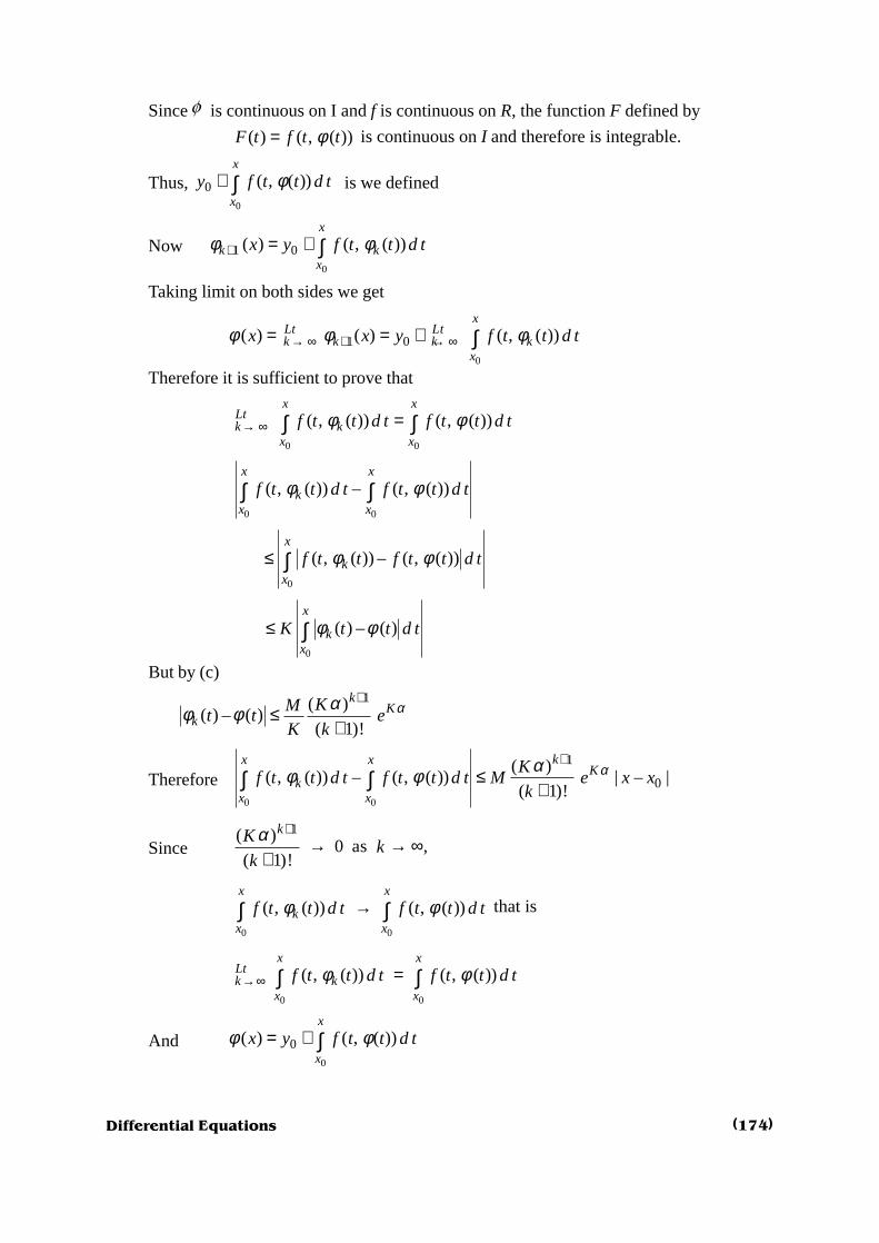
Differential Equations
Since f is continuous on I and f is continuous on R, the function F defined by
( ) ( , ( ))F t f t tφ= is continuous on I and therefore is integrable.
Thus, 0
0 ( , ( ))x
x
y f t t d tφ+ ∫ is we defined
Now 0
1 0( ) ( , ( ))x
k kx
x y f t t d tφ φ+ = + ∫
Taking limit on both sides we get
0
1 0( ) ( ) ( , ( ))φ φ φ→ ∞ + → ∞= = + ∫x
Lt Ltk k k k
x
x x y f t t d t
Therefore it is sufficient to prove that
0 0
( , ( )) ( , ( ))x x
Ltk k
x x
f t t d t f t t d tφ φ→ ∞ =∫ ∫
0 0
( , ( )) – ( , ( ))∫ ∫x x
kx x
f t t d t f t t d tφ φ
0
( , ( )) – ( , ( ))φ φ≤ ∫x
kx
f t t f t t d t
0
( ) – ( )x
kx
K t t d tφ φ≤ ∫
But by (c)
1( )
( ) – ( )( 1)!
+≤
+
kK
kKM
t t eK k
ααφ φ
Therefore0 0
1
0( )
( , ( )) – ( , ( )) | – |( 1)!
+≤
+∫ ∫kx x
Kk
x x
Kf t t d t f t t d t M e x x
kααφ φ
Since1( )
0 as ,( 1)!
+→ → ∞
+
kKk
k
α
0 0
( , ( )) ( , ( ))x x
kx x
f t t d t f t t d tφ φ→∫ ∫ that is
0 0
( , ( )) ( , ( ))φ φ→∞ =∫ ∫x x
Ltk k
x x
f t t d t f t t d t
And 0
0( ) ( , ( ))x
x
x y f t t d tφ φ= + ∫
(174)

Differential Equations
Thus f is a solution of the initial value problem 0 0( , ), ( )y f x y y x y′ = = on I.
In theorem 4.2.1 we have shown the existence of solution of initial value problem 4.1.1.The solution thus obtained is a uniques solution.
Picard-Lindel of theorem states that if f is continuous function and satisfies Lipschitz conditionon R, then the successive approximations fk exist on |x – x0 | £ a , fk’s are continuous andconverge uniformaly on the interval I to a unique solution passing through (x0, y0) ÎR.
S
(175)

Differential Equations
References
1. Earl A coddington, An introduction to ordinarydifferential equations : Prentice Hall of India, New Delhi1995.
2. Morris Tenenbaum and Harry Pollard, Ordinarydifferential Equations : New York 1963
3. Gorett Birkhoff, Gian-Carlo Rota, Ordinary differentialequations : John Wiley and Sons, New York 1978
4. Earl D Rainville, Elementory differential Equations,Macmillan Company New York 1964

1
GREEN’S FUNCTION AND STURM-LIOUVILLE THEORY
CHAPTER : 5
1. Green’s Functions :
Given the inhomogeneous linear second-order differential equation
2
2( ) ( ) ( ) ( )= + + =d u du
L u p x q x u r xdxdx
, .... (1)
we will show that there exists an integral operator G defined by,
( ) ( )( ) ,= ∫x
a
G r G x r dξ ξ ξ ... (2)
Such that ( )( ) =L G r r
The Kernel ( ),G x ξ of equation (2) is called the Green’s function associated with given initial
value problem or boundary value problem.
For the initial value problem of nth order we have following definition for Green’s function.
Definition 1.1 :
Let 1
1 1( ) ( ) .... ( )−
−= + + +n n
nn n
d u d uL u p x p x u
dx dx, be an nth order homogeneous linear differential
operator. By the Green’s function of L (u) for the initial value problem at x = a is meant a function
( ),G x ξ such that the function defined by ( ) ( )( ) ( ) ,= = ∫x
a
u x G r G x r dξ ξ ξ satisfies ( ) ( )=L u r x ,
for any continuous function ( )r x , and satisfies the initial conditions ( )1( ) '( ) .... ( ) 0−= = = =nu a u a u a .
Theorem 1.1
Let the function ( ),G t τ be defined as follows :
(i) ( ), 0=G t τ , for ≤ ≤a t τ ,
(ii) for each fixed ≥ aτ , and all >t τ , ( ),G t τ is the solution of the differential equation.
( ) ( ) ( ) 0= + + =tt tL G G p t G q t G
which satisfies the initial conditions,

3
Therefore,
( ) ( )( ) , ( )′′ = +∫t
tta
u t G t t d r tτ τ τ ..... (5)
Thus using (3), (4) and (5) we have
( ) ( ) ( ) ( ) ( ) ( )′′ ′= + +L u u t p t u t q t u t
( ) ( ) ( ) ( ) ( ) ( ), ( ) ( ) , ( ) ,= + + +∫ ∫ ∫t t t
tt ta a a
G t r d r t p t G t r d q t G t r dτ τ τ τ τ τ τ τ τ
( ) ( ) ( ) ( ) ( ) ( ), ( ) ( ) , ( ) ,t t t
tt ta a a
G t r d r t p t G t r d q t G t r dτ τ τ τ τ τ τ τ τ= + + +∫ ∫ ∫
( ) ( ) ( ), ( ) , ( ) , ( )= + + + ∫t
tt ta
G t p t G t q t G t d r tτ τ τ τ .... (6)
But by condition in (ii) ( ),G t τ satisfy
( ) ( ) 0+ + =tt tG p t G q y G
Thus equation (6) becomes
( ) ( )=L u r t
This proves that the function u defined by (3) is the solution of second order differential equation(1).
Theorem 1.2 : The solution of inhomogeneous second order differential equation
2
2( ) ( ) ( ) ( )d u du
L u p x q x u r xdxdx
= + + =
for the initial conditions ( ) ( ) 0′= =u a u a , is
( ) ( )( ) ,= ∫t
a
u t G t t dτ τ τ
where
( ) ( )( )
( ) ( )( , )
( , )
−=
f g t g f tG t
W f g
τ ττ
τ
and ( )( , )W f g τ is the Wronskian of two linearly independent solutions f and g of the homogeneous
equation.

5
From (2) and conditions in (4) we obtain
( ) ( ) ( ) ( ) 0c f d gτ τ τ τ+ =
and ( ) ( ) ( ) ( ) 1c f d gτ τ τ τ′ ′+ =
Solving these simultaneous linear equations we obtain
( )
( )( )
( ) ( )( ) ( )
( )( )
0
1( , )
'
ggg
cW f gf g
f g
τττ
τττ τ
τ τ
′= = −
′
and( )
( )( )
( ) ( )( ) ( )
( )( )
0
1( , )
′= =
′ ′
fff
dW f gf g
f g
τττ
τττ τ
τ τ
Thus from (2) the required Green’s function si,
( )( )
( )( )
( ), ( ) ( )
( , ) ( , )
−= +
g fG t f t g t
W f g W f g
τ ττ
τ τ
( ) ( ) ( )( )
( )
( , )
−=
f g t g f t
W f g f
τ τ
τ.... (5)
Hence the solution of
( ) ( ) ( ) ( )′′ ′= + + =L u u p x u q x u r x
is ( ) ( )( ) ,= ∫t
a
u t G t t dτ τ τ ... (6)
where ( , )G t τ is given in (5).
Remark : In the elementary theory of differential equations formula (6) is often derived formally byposing the question : What must be ( )c τ and ( )d τ be in order that the function
( ) ( )( , ) ( ) ( )G t c f t d g tτ τ τ= +
when substituted into (6), should give the solution of the homogeneous differential equation
( )( ) ( )=L u t r t
Since ( )c τ and ( )d τ may be regarded as ‘variable parameters’, which vary with τ , formula(6) is said to be obtained by the method of variation of parameters.

7
function is given by
( )( ) ( )
( )( ) ( )
,( , )
−=
f g t g f tG t
W f g
τ ττ
τ
( ) ( )( ) ( )( ) ( )
( ) ( )−=
′ ′
f g t g f t
f gf g
τ τ
τ ττ τ
cos sin sin coscos sinsin cos
−=
−
t tτ ττ ττ τ
( )2 2
sin
cos sin
−=
+
t τ
τ τ
( )sin= −t τ
Problem 1.2 : Integrate the following differential equations by constructing Green’s functions.
(a) 10 25 sin′′ ′+ + =y y y x
(b) 4 16 15y y y x′′ ′− + =
(c) 2 −′′ ′− − = xy y y e
Solution :
(a) Given differential equation is
10 25 sin′′ ′+ + =y y y x ... (1)
The characteristic polynomial is
2 2( ) 10 25 ( 5)= + + = +p r r r r
and its roots are r = – 5, – 5.
Thus two linearly independent solutions are 5( ) −= xf x e , 5( ) −= xg x xe . The solution of
differential equation (1) is given by
( ) ( )( ) ,= ∫t
y t G t r dτ τ τ ..... (2)
where ( ) sin=r τ τ and ( ),G t τ is Green’s function defined by
( )( ) ( )
( )( ) ( )
,( , )
−=
f g t g f tG t
W f g
τ ττ
τ

9
5 55 55
sin cos26 26
t tte ee e dτ ττ τ τ
− −
= −∫ ∫
( ) [ ]5 5 5 55
5sin cos 5cos sin26 26 26 25 1
− −
= − − ++
t t t te e e et t t t
( ) [ ]5 15sin cos 5cos sin
676 676= − − +t t t t
[ ]125sin 5cos 5cos sin
676= − − −t t t t
[ ]124sin 10cos
676= −t t
12sin 5cos
338
−=
t t
is the required solution of (1).
(b) The characteristic polynomial of the equation
4 16 15y y y x′′ ′− + = .... (1)
is 2( ) 4 16 15p r r r= − +
24 10 6 15r r r= − − +
2 (2 5) 3(2 5)r r r= − − −
(2 3)(2 5)r r= − −
and its roots are
3 5,
2 2r =
The two linearly independent solutions are 3
2( )x
f x e= and 5
2( )x
g x e= .
The solution differential equation (1) is given by
( ) ( )( ) ,= ∫t
y t G t r dτ τ τ .... (2)

11
where ( ) −=r e ττ and
( )( ) ( )
( )( ) ( )
,( , )
−=
f g t g f tG t
W f g
τ ττ
τ
( ) ( )( ) ( ) ( ) ( )
( ) ( )−=
′ ′−
f f t g f t
f g g f
τ τ
τ τ τ τ
2 2
2 2(2) ( 1)
− −
− −
−=
− −
t te e e e
e e e e
τ τ
τ τ τ τ
2 2
2
− −−=
+
t te e e e
e e
τ τ
τ τ
[ ]2 21
3− −= −t te e e eτ τ
Thus equation (1) reduces to
[ ]2 21( )
3− − −= −∫
tt ty t e e e e e dτ τ τ τ
[ ]3 21
3− −= −∫
tt te e e dτ τ
3
21
3 ( 3)
−−
= −
− t te
e e tτ
1
9 3
−−= − −
tt te
e
is the required solution.
EXERCISE
1. Construct Green’s function for the initial value problem, for the following differential equations.
(a) 4 0′′ + =y y
(b) 0′′ + =y y
(c) 3 2 0′′ ′+ + =y y y

13
( ) ( ) ( ) 0d du
p x q x u r x udx dx
λ
+ + = , a x b≤ ≤
Coupled with boundary conditions.
( ) ( )u a u b= , ( ) ( )u a u b′ ′= .... (3)
is called a periodic Sturm-Liouville boundary value problem.
Definition 2.5 : A noutrivial solution of Sturm-Liouville boundary value problem (BVP) is called aneigen function and the corresponding λ is called its eigen value.
For a value of λ if xλ is non trivial solution of Sturm-Liouville BVP then λ is an eigen value
and xλ is eigen function corresponding to λ .
Definition 2.6 : The set of all eigen values of regular Sturm-Liouville BVP is called the spectrum ofthe Sturm-Liouville BVP.
Theorem 2.1: Let u and v be two eigen functions of Sturm-Liouville BVP
( ) ( ) ( ) 0d du
p x q x u r x udx dx
λ
+ + = , a x b≤ ≤
1 1( ) ( ) 0u a u aα β ′+ = ... (2.1)
2 2( ) ( ) 0u a u bα β ′+ = .... (2.2)
Corresponding to eigen values λ and µ . Then
[ ]( , ) 0bap W u v = , .... (3)
where W (u, v) is the Wronskian of u and v.
If p (a) = 0 then (3) holds without use of (2.1).
If p (b) = 0 then (3) holds without use of (2.2).
Proof : Let ( ) 0p a ≠ and ( ) 0p b ≠ .
As u and v are the eigen functions of the Sturm-Liouville problem, from (2.1) we have
1 1( ) ( ) 0u a u aα β ′+ =
and 1 1( ) ( ) 0v a v aα β ′+ =
By definition of Sturm-Liouville BVP, at least one of 1α and 1β is non-zero.
Let us suppose 1 0α ≠ .
Elimination of 1β from above two equations leads to
[ ]1 ( ) ( ) ( ) ( ) 0u a v a v a u aα ′ ′− =

15
Proof : Let u and v be two eigen functions of periodic Strum-Liouville BVP (1) - (2).
Then p (a) = p (b) and in this case we have
[ ]( ) ( ( ), ( ))bap x W u x v x
( )( ) ( ) ( ) ( ) ( )b
ap x u x v x v x u x′ ′ = −
[ ] [ ]( ) ( ) ( ) ( ) ( ) ( ) ( ) ( ) ( ) ( )p b u b v b v b u b p a u a v a v a u a′ ′ ′ ′= − − −
[ ]( ) ( ) ( ) ( ) ( ) ( ) ( ) ( ) ( )p b u b v b v b u b u a v a v a u a′ ′ ′ ′= − − +
The expression inside the bracket is zero once we use the periodic conditions.
( ) ( ) ( ) ( )u a u b u a u b′ ′= = −
and ( ) ( ), ( ) ( )v a v b v a v b′ ′= =
Thus [ ]( , ) 0bapW u v =
Definition 2.7 : Two integrable real-valued functions f and g are orthogonal with weight function
( ) 0r t > on an interval [ a, b] if and only if ( ) ( ) ( ) 0b
a
r x f x g x dx =∫ .
Theorem 2.3 : The eigen functions of a regular Sturm-Liouville BVP corrosponding to distinct eigenvalues are orthogonal on an interval [a, b] with weight function r.
Proof : Let u and v be the eigen functions corresponding to distinct eigen values λ and u, of a regularSturm-Liouville problem.
( ) ( ) ( ) 0, d du
p x q x u r x u a x bdx dx
λ
+ + = ≤ ≤ .... (1)
1 1( ) ( ) 0u a u aα β ′+ = .... (2.1)
2 2( ) ( ) 0u b u bα β ′+ = .... (2.2)
Then from (1) we have
( ) ( ) ( ) 0d du
p x q x u r x udx dx
λ
+ + = .... (3)
and
( ) ( ) ( ) 0d dv
p x q x v r x vdx dx
λ
+ + = ... (4)

17
Taking complex conjugate of (1), we get
( ) ( ) ( ) 0d du
p x q x u r x udx dx
λ
+ + = .... (2)
Multiply the differential equation in (1) by u , and multiply that of (2) by u, and substractingone from other we get,
( )( ) ( ) ( ) 0d du d du
p x u p x u r x uudx dx dx dx
λ λ
− + − =
( ) ( ) ( )d du du
r x uu p x u udx dx dx
λ λ
− = −
( )( ) ( ), ( )d
p x W u x u xdx
=
Integrating the last equality, we get
( ) ( )( ) ( ) ( ) ( ) ( ), ( )b
b
aa
r x u x u x dx p x W u x u xλ λ − = ∫ .... (3)
Since u and u satisfy the boundary conditions (2.1) and (2.2), we have
( )( ) ( ), ( ) 0b
ap x W u x u x =
Thus (3) reduces to
( ) 2( ) ( ) 0
b
a
r x u x dxλ λ− =∫ .... (4)
Since u, being an eigen function, is not identically equal to zero and ( ) 0r x > on [a, b], wehave
2( ) ( ) 0
b
a
r x u x dx ≠∫
Therefore, from (4), λ λ= . That is, λ is real.
Problem 2.1 : Show that the boundary value problem
( ) ( ) 0, (0) 0, (1) 0u x u x u uλ′′ ′+ = = =
is a Sturm-Liouville problem, and find all eigen values and a corrosponding set ofeigen functions.

19
Thus the general solution is
1 2( ) x xu x C e C eµ µ−= +
1 2( ) x xu x C e C eµ µµ µ −′⇒ = −
Applying boundary conditions, we get
1 2 2 10 (0)u C C C C= = + ⇒ = −
1 10 (1) 0u C e C eµ µµ µ −′= = + = 1
10
⇒ + =
C e
eµ
µµ
Since 0µ ≠ , 1
0ee
µµ+ ≠ , we have C1 = 0.
So again the only solution is zero solution, therefore there are no negative eigenvalues.
Case 3 : Let 0λ > . Assume 2λ µ= , for some non zero real µ .
The characteristic polynomial becomes2 2 0r µ+ =
r iµ⇒ = ±
The general solution in this case is
1 2( ) cos sinu x C x C xµ µ= +
Using boundary conditions we get
10 (0)u C= =
Therefore,
2( ) sinu x C xµ=
2( ) cosu x C xµ µ′⇒ =
Using boundary condition, we get
20 (1) cosu C µ µ′= =
Since 0µ ≠ , 2 0C = again gives trivial solution. Thus we assume 2 0C ≠ .
This give cos 0µ = .
This is true for ( )2 1
2nn π
µ+
= , n = 0, 1, 2, .....
Therefore the eigen values are
( ) 22 2 1
2n n
n πλ µ
+ = =
, n = 0, 1, 2, .....

21
Solving (1) and (2) we get
1 0C = , 2 0C = .
Thus, only soloution in this case is the trivial solution ( ) 0u x = . Therefore there are no negativeeigen values.
Case 3 : Let 0λ > . Assume 2λ µ= , where µ is real nonzero real number. Then the characteristic
polynomial is
2 2 0r µ+ =
r iµ⇒ = ±
Therefore the general solution is
1 2( ) cos sinu x C x C xµ µ= +
1 2( ) sin cosu x C x C xµ µ µ µ′⇒ = − +
The condition (0) ( )u u π= gives that
1 1 2cos sinC C Cµπ µπ= +
( ) ( )1 21 cos sin 0C Cµπ µπ⇒ − − = .... (3)
Further the condition (0) ( )u u π′ ′= gives
2 1 2sin cosC C Cµπ µπ= − +
( ) ( )1 2sin 1 cos 0C Cµπ µπ⇒ + − = .... (4)
The system (3) and (4) has non trivial solution for C1 and C2 if and only if
1 cos sin0
sin 1 cosµπ µπ
µπ µπ− −
=−
( )2 21 cos sin 0µπ µπ⇒ − + =
2 21 2cos cos sin 0µπ µπ µπ⇒ − + + =
2 2cos 0µπ⇒ − =
cos 1µπ⇒ =
2n nµ⇒ = ± , n = 1, 2, 3, .....
Thus positive eigen values are given by
2 24n n nλ µ= = , n = 1, 2, 3, .....

23
2 2
2(log2)n
n πλ⇒ = , n = 1, 2, 3 ....
are the required eigen values and corrosponding eigen function is
( ) sin loglog2nn
u x xπ
=
, n = 1, 2, 3, ......
Problem 2.4 : Show that the eigen values of Sturm-Liouville BVP
( ) ( ) 0u x u xλ′′ + = , 0 x L≤ ≤
(0) 0u = , ( ) 0u L =
are all positive.
Solution : The equation Sturm-Liouville equation is
( ) ( ) 0u x u xλ′′ + =
Multiplying this equation by ( )u x and then integrating from 0 to L, we obtain
22
20 0
( ) ( ) 0L Ld uu x dx u x dx
dxλ+ =∫ ∫
2
0 0 0
( ) ( ) 0L L Ldu du du
u x dx u x dxdx dx dx
λ
⇒ − + = ∫ ∫
As (0) 0u = and ( ) 0u L = , above equation reduces to
22
0 0
( ) 0L Ldu
dx u x dxdx
λ
− + = ∫ ∫
2
0
2
0
( ) 0
L
L
dudx
dx
u x dx
λ
⇒ =
=
∫
∫
As integrands of both the integrals are non-negative, we must have 0λ ≥ .

25
Writting Team Chapter Number
Dr. (Mrs.) Sarita Thakar
Department of Mathematics, 1 – 4
Shivaji University, Kolhapur.
Maharashtra
Dr. Kishor D. Kucche
Department of Mathematics, 5
Shivaji University, Kolhapur.
Maharashtra