Electron Transfer Reactions: a Treatise - Scientific & Academic ...
Upload
khangminh22Category
view
2download
0

Digitized by the Internet Archive
in 2007 with funding from
Microsoft Corporation
http://www.archive.org/details/elementarytreatiOOpiaguoft


BELL'S MATHEMATICAL SERIESADVANCED SECTION ( £(-*
General Editor-. WILLIAM P. MILNE, M.A., D.Sc^Professor of Mathematics, Leeds University
AN ELEMENTARY TREATISEON DIFFERENTIAL EQUATIONS AND
THEIR APPLICATIONS
y

G. BELL AND SONS, LTD.LONDON : PORTUGAL ST., KINGSWAY
CAMBRIDGE : DEIGHTON, BELL & CO.
NEW YORK : THE MACMILLAN COM-
PANY BOMBAY : A. H. WHEELER & CO.

AN ELEMENTARY TREATISE ON
DIFFERENTIALEQUATIONS
AND THEIR APPLICATIONS
BY
H. T. H. PIAGGIO, M.A., D.Sc.
PROFESSOR OF MATHEMATICS, UNIVERSITY COLLEGE, NOTTINGHAMFORMERLY SENIOR SCHOLAR OF ST. JOHN'S COLLEGE, CAMBRIDGE
\^*jk\
V
LONDONG. BELL AND SONS, LTD.
1920
V
3D?5
Glasgow: printed at the university press
by robert maclehose and co. ltd.
PREFACE
" The Theory of Differential Equations," said Sophus Lie, " is the
most important branch of modern mathematics." The subject maybe considered to occupy a central position from which different
lines of development extend in many directions. If we travel along
the purely analytical path, we are soon led to discuss Infinite Series,
Existence Theorems and the Theory of Functions. Another leads
us to the Differential Geometry of Curves and Surfaces. Between
the two lies the path first discovered by Lie, leading to continuous
groups of transformation and their geometrical interpretation.
Diverging in another direction, we are led to the study of mechanical
and electrical vibrations of all kinds and the important phenomenon
of resonance. Certain partial differential equations form the start-
ing point for the study of the conduction of heat, the transmission
of electric waves, and many other branches of physics. Physical
Chemistry, with its law of mass-action, is largely concerned with
certain differential equations.
The object of this book is to give an account of the central
parts of the subject in as simple a form as possible, suitable for
those with no previous knowledge of it, and yet at the same time
to point out the different directions in which it may be developed.
The greater part of the text and the examples in the body of it
will be found very easy. The only previous knowledge assumed is
that of the elements of the differential and integral calculus and a
little coordinate geometry. The miscellaneous examples at the end
of the various chapters are slightly harder. They contain several
theorems of minor importance, with hints that should be sufficient
to enable the student to solve them. They also contain geometrical
and physical applications, but great care has been taken to state
the questions in such a way that no knowledge of physics is required.
For instance, one question asks for a solution of a certain partial
vi PREFACE
differential equation in terms of certain constants and variables.
This may be regarded as a piece of pure mathematics, but it is
immediately followed by a note pointing out that the work refers
to a well-known experiment in heat, and giving the physical meaning
of the constants and variables concerned. Finally, at the end of
the book are given a set of 115 examples of much greater difficulty,
most of which are taken from university examination papers. [I
have to thank the Universities of London, Sheffield and Wales, and
the Syndics of the Cambridge University Press for their kind per-
mission in allowing me to use these.] The book covers the course
in differential equations required for the London B.Sc. Honours or
Schedule A of the Cambridge Mathematical Tripos, Part II., and
also includes some of the work required for the London M.Sc. or
Schedule B of the Mathematical Tripos. An appendix gives sugges-
tions for further reading. The number of examples, both worked
and unworked, is very large, and the answers to the unworked ones
are given at the end of the book.
A few special points may be mentioned. The graphical method
in Chapter I. (based on the MS. kindly lent me by Dr. Brodetsky
of a paper he read before the Mathematical Association, and on a
somewhat similar paper by Prof. Takeo Wada) has not appeared
before in any text-book. The chapter dealing with numerical
integration deals with the subject rather more fully than usual.
It is chiefly devoted to the methods of Runge and Picard, but it
also gives an account of a new method due to the present writer.
The chapter on linear differential equations with constant co-
efficients avoids the unsatisfactory proofs involving " infinite con-
stants." It also points out that the use of the operator D in finding
particular integrals requires more justification than is usually given.
The method here adopted is at first to use the operator boldly and
obtain a result, and then to verify this result by direct differentiation.
This chapter is followed immediately by one on Simple Partial
Differential Equations (based on Riemann's " Partielle Differential -
gleichungen "). The methods given are an obvious extension of
those in the previous chapter, and they are of such great physical
importance that it seems a pity to defer them until the later portions
of the book, which is chiefly devoted to much more difficult subjects.
In the sections dealing with Lagrange's linear partial differential
equations, two examples have been taken from M. J. M. Hill's
recent paper to illustrate his methods of obtaining special integrals.

PREFACE vii
In dealing with solution in series, great prominence has been
given to the method of Frobenius. One chapter is devoted to the
use of the method in working actual examples. This is followed
by a much harder chapter, justifying the assumptions made and
dealing with the difficult questions of convergence involved. Aneffort has been made to state very clearly and definitely where the
difficulty lies, and what are the general ideas of the somewhat
complicated proofs. It is a common experience that many students
when first faced by a long " epsilon-proof " are so bewildered by
the details that they have very little idea of the general trend.
I have to thank Mr. S. Pollard, B.A., of Trinity College, Cambridge,
for his valuable help with this chapter. This is the most advanced
portion of the book, and, unlike the rest of it, requires a little know-
ledge of infinite series. However, references to standard text-books
have been given for every such theorem used.
I have to thank Prof. W. P. Milne, the general editor of Bell's
Mathematical Series, for his continual encouragement and criticism,
and my colleagues Mr. J. Marshall, M.A., B.Sc, and Miss H. M.
Browning, M.Sc, for their work in verifying the examples and
drawing the diagrams.
I shall be very grateful for any corrections or suggestions from
those who use the book.
H. T. H. PIAGGIO.
University College, Nottingham,
February, 1920.


CONTENTS
Historical IntroductionPAOK
XV
CHAPTER I
INTRODUCTION AND DEFINITIONS. ELIMINATION.GRAPHICAL REPRESENTATION
ART.
1-3. Introduction and definitions 1
4-6. Formation of differential equations by elimination - - 2
7-8. Complete Primitives, Particular Integrals, and Singular
Solutions 4
9. Brodetsky and Wada's method of graphical representation - 5
10. Ordinary and Singular points 7
Miscellaneous Examples on Chapter I - - - - 10
CHAPTER II
EQUATIONS OF THE FIRST ORDER AND FIRST DEGREE
11. Types to be considered 12
12. Exact equations 12
13. Integrating factors 13
14. Variables separate ........ 13
15-17. Homogeneous equations of the first order and degree - - 14
18-21. Linear equations of the first order and degree - - - 16
22. Geometrical problems. Orthogonal trajectories - - - 19
Miscellaneous Examples on Chapter II - - - 22
CHAPTER III
LINEAR EQUATIONS WITH CONSTANT COEFFICIENTS
23. Type to be considered -
24. Equations of the first order
25
25

CONTENTS
ART.
25. Equations of the second order
26. Modification when the auxiliary equation has imaginary or
complex roots
27. The case of equal roots-••---..28. Extension to higher orders -
29. The Complementary Function and the Particular Integral -
30-33. Properties of the operator D34. Complementary Function when the auxiliary equation has
repeated roots
35-38. Symbolical methods of finding the Particular Integral. Ten-tative methods and the verification of the results they give
39. The homogeneous linear equation
40. Simultaneous linear equations ------Miscellaneous Examples on Chapter III. (with notes on
mechanical and electrical interpretations, free andforced vibrations and the phenomenon of resonance)
CHAPTER IV
SIMPLE PARTIAL DIFFERENTIAL EQUATIONS
41. Physical origin of equations to be considered
42-43. Elimination of arbitrary functions and constants -
44. Special difficulties of partial differential equations -
45-46. Particular solutions. Initial and boundary conditions -
47-48. Fourier's Half-Range Series
49-50. Application of Fourier's Series in forming solutions satisfying
given boundary conditions ------Miscellaneous Examples on Chapter IV. (with notes on
the conduction of heat, the transmission of electric
waves and the diffusion of dissolved salts)
CHAPTER V
EQUATIONS OF THE FIRST ORDER, BUT NOT OF THEFIRST DECREE
51. Types to be considered-----...52. Equations solvable for p
53. Equations solvable for y
54. Equations solvable for x

CONTENTS XI
CHAPTER VI
SINGULAR SOLUTIONSART. PAGE
55. The envelope gives a singular solution ----- 6">
56-58. The c-discriroinant contains the envelope (once), the node-
locus (twice), and the cusp-locus (three times) 60
59-64. The ^-discriminant contains the envelope (once), the tac-locus
(twice), and the cusp-locus (once) - - - - - 71
65. Examples of the identification of loci, using both discriminants 75
66-67. Clairaut's form:
- - 76
Miscellaneous Examples on Chapter VI - - - - 78
CHAPTER VII
MISCELLANEOUS METHODS FOR EQUATIONS OF THESECOND AND HIGHER ORDERS
68. Types to be considered 81
69-70. y or x absent 82
71-73. Homogeneous equations 83
74. An equation occurring in Dynamics 85
75. Factorisation of the operator - - - - - - 86
76-77. One integral belonging to the complementary function known 87
78-80. Variation of Parameters 88
81. Comparison of the different methods ----- 90
Miscellaneous Examples on Chapter VII. (introducing the
Normal form, the Invariant of an equation, and the
Schwarzian Derivative) 91
CHAPTER VIII
NUMERICAL APPROXIMATIONS TO THE SOLUTION OFDIFFERENTIAL EQUATIONS
82. Methods to be considered ------- 94
83-84. Picard's method of integrating successive approximations - 94
85. Numerical approximation direct from the differential equa-
tion. Simple methods suggested by geometry 97
86-87. Runge's method 99
88. Extension to simultaneous equations 103
89. Methods of Heun and Kutta 104
90-93. Method of the present writer, with limits for the error - - 105

xii CONTENTS
CHAPTER IX
SOLUTION IN SERIES. METHOD OF FROBENIUSART. PAOK
94. Frobenius' form of trial solution. The indicia] equation - 109
95. Case I. Roots of indicial equation unequal and differing by a
quantity not an integer - - 110
96. Connection between the region of convergence of the series
and the singularities of the coefficients in the differential
equation 112
97. Case II. Roots of indicial equation equal - - - - 112
98. Case III. Roots of indicial equation differing by an integer,
making a coefficient infinite - - - -. - - 114
99. Case IV. Roots of indicial equation differing by an integer,
making a coefficient indeterminate 116
100. Some cases where the method fails. No regular integrals - 117
Miscellaneous Examples on Chapter IX. (with notes on
the hypergeometric series and its twenty-four solu-
tions) 119
CHAPTER X
EXISTENCE THEOREMS OF PICARD, CAUCHY, ANDFROBENIUS
101. Nature of the problem 121
102. Picard's method of successive approximation - - - 122
103-105. Cauchy's method 124
106-110. Frobenius' method. Differentiation of an infinite series with
respect to a parameter - - - - - - -127
CHAPTER XI
ORDINARY DIFFERENTIAL EQUATIONS WITH THREEVARIABLES AND THE CORRESPONDING CURVES
AND SURFACES
111. The equations of this chapter express properties of curves and
surfaces 133
112. The simultaneous equations dx/P=dylQ=dz/R • - - 133
113. Use of multipliers 135
114. A second integral found by the help of the first - - - 136
115. General and special integrals 137

CONTENTS xiii
ART. FAOB
116. Geometrical interpretation of the equation
Pdx+Qdy + Rdz=0 - - - - 137
117. Method of integration of this equation when it is integrable - 138
118-119. Necessary and sufficient condition that such an equation
should be integrable 139
120. Geometrical significance of the non-integrable equation - 142
Miscellaneous Examples on Chapter XI - - - 143
CHAPTER XII •
PARTIAL DIFFERENTIAL EQUATIONS OF THE FIRST
ORDER. PARTICULAR METHODS
121-122. Equations of this chapter of geometrical interest - - - 146
123. Lagrange's linear equation and its geometrical interpretation 147
124. Analytical verification of the general integral - - - 149
125. Special integrals. Examples of M. J. M. Hill's methods of
obtaining them 150
126-127. The linear equation with n independent variables - - - 16*1
128-129. Non-linear equations. Standard I. Only p and q present - 153
130. Standard II. Only p, q, and z present 153
131. Standard III. f(x, p)=F(y, q) 154
132. Standard IV. Partial differential equations analogous to
Clairaut's form 154
133-135. Singular and General integrals and their geometrical signifi-
cance. Characteristics 155
136. Peculiarities of the linear equation 158
Miscellaneous Examples on Chapter XII. (with a note onthe Principle of Duality) 160
CHAPTER XIII
PARTIAL DIFFERENTIAL EQUATIONS OF THE FIRSTORDER. GENERAL METHODS
137. Methods to be discussed 162
138-139. Charpit's method 162
140-141. Three or more independent variables. Jacobi's method - 165
142. Simultaneous partial differential equations - 168
Miscellaneous Examples on Chapter XIII - - - 170

xiv CONTENTS
CHAPTER XIV
PARTIAL DIFFERENTIAL EQUATIONS OF THE SECONDAND HIGHER ORDERS
ART. PAQ
143. Types to be considered 171]
144. Equations that can be integrated by inspection. Determina-
tion of arbitrary functions by geometrical conditions - 17!
145-151. Linear partial differential equations with constant coefficients 171.
152-153. Examples in elimination, introductory to Monge's methods - 17!>
154. Monge's method of integrating Rr + Ss + Tt = V - - - 181
155. Monge's method of integrating Rr + Ss + Tt + U(rt -s-) = V - 18.'!
156-157. Formation of Intermediate Integrals 183
158. Further integration of Intermediate Integrals - - - 186
Miscellaneous Examples on Chapter XIV. (with notes onthe vibrations of strings, bars, and membranes, andon potential) 188
APPENDIX ANecessary and sufficient condition that the equation
Mdx+Ndy=0should be exact - - 191
APPENDIX BAn equation with no special integrals ----- 192
APPENDIX C
The equation found by Jacobi's method .of Art. 140 is
always integrable -----... 193
APPENDIX DSuggestions for further reading -----.. 194
Miscellaneous Examples <>n the Whole Book (withnotes on solution by definite intregals, asymptotic series,
the Wronskian, Jacobi's last multiplier, finite difference
equations, Hamilton's dynamical equations, Foueault's
pendulum, and the perihelion of Mercury) - - . 195
Answers t<> the Examplesj
,S|JKXxxiii

HISTORICAL INTRODUCTION
The study of Differential Equations began very soon after the
invention of the Differential and Integral Calculus, to which it
forms a natural sequel. Newton in 1676 solved a differential
equation by the use of an infinite series, only eleven years after
his discovery of the fluxional form of the differential calculus in
1665. But these results were not published until 1693, the same
year in which a differential equation occurred for the first time in
the work of Leibniz * (whose account of the differential calculus
was published in 1684).
In the next few years progress was rapid. In 1694-97 John
Bernoulli f explained the method of " Separating the Variables," and
he showed how to reduce a homogeneous differential equation of
the first order to one in which the variables were separable. Heapplied these methods to problems on orthogonal trajectories. Heand his brother Jacob ft (after whom " Bernoulli's Equation " is
named) succeeded in reducing a large number of differential equa-
tions to forms they could solve. Integrating Factors were probably
discovered by Euler (1734) and (independently of him) by Fontaine
and Clairaut, though some attribute them to Leibniz. Singular
Solutions, noticed by Leibniz (1694) and Brook Taylor (1715), are
generally associated with the name of Clairaut (1734). The geo-
metrical interpretation was given by Lagrange in 1774, but the
theory in its present form was not given until much later by Cayley
(1872) and M. J. M. Hill (1888).
The first methods of solving differential equations of the second
or higher orders with constant coefficients were due to Euler.
D'Alembert dealt with the case when the auxiliary equation had
equal roots. Some of the symbolical methods of finding the par-
ticular integral were not given until about a hundred years later
by Lobatto (1837) and Boole (1859).
The first partial differential equation to be noticed was that
giving the form of a vibrating string. This equation, which is of
the second order, was discussed by Euler and D'Alembert in 1747.
Lagrange completed the solution of this equation, and he also
* Also spelt Leibnitz. f Also spelt Bcrnouilli. ft Also known as James.
xv

XVI HISTORICAL INTRODUCTION
dealt, in a series of memoirs from 1772 to 1785, with partial dif-
ferential equations of the first order. He gave the general integral
of the linear equation, and classified the different kinds of integrals
possible when the equation is not linear.
These theories still remain in an unfinished state ; contributions
have been made recently by Chrystal (1892) and Hill (1917). Other
methods for dealing with partial differential equations of the first
order were given by Charpit (1784) and Jacobi (1836). For higher
orders the most important investigations are those of Laplace (1773),
Monge (1784), Ampere (1814), and Darboux (1870).
By about 1800 the subject of differential equations in its original
aspect, namely the solution in a form involving only a finite numberof known functions (or their integrals), was in much the same state
as it is to-day. At first mathematicians had hoped to solve every
differential equation in this way, but their efforts proved as fruitless
as those of mathematicians of an earlier date to solve the general
algebraic equation of the fifth or higher degree. The subject nowbecame transformed, becoming closely allied t<5 the Theory of
Functions. Cauchy in 1823 proved that the infinite series obtained
from a differential equation was convergent, and so really did
define a function satisfying the equation. Questions of convergency
(for which Cauchy was the first to give tests) are very prominent
in all the investigations of this second period of the study of dif-
ferential equations. Unfortunately this makes the subject very
abstract and difficult for the student to grasp. In the first period
the equations were not only simpler in themselves, but were studied
in close connection with mechanics and physics, which indeed were
often the starting point of the work.
Cauchy's investigations were continued by Briot and Bouquet
(1856), and a new method, that of " Successive Approximations,"
was introduced by Picard (1890). Fuchs (1866) and Frobenius
(1873) have studied linear equations of the second and higher
orders with variable coefficients. Lie's Theory of Continuous
Groups (from 1884) has revealed a unity underlying apparently
disconnected methods. Schwarz, Klein, and Goursat have madetheir work easier to grasp by the introduction of graphical con-
siderations, and a recent paper by Wada (1917) has given a graphical
representation of the results of Picard and Poincarr. Runge (1895)
and others have dealt with numerical approximations.
Further historical notes will be found in appropriate places
throughout the book. For more detailed biographies, see Rouse
Ball's Short History of Mathematics.

CHAPTER I
INTRODUCTION AND DEFINITIONS. ELIMINATION.GRAPHICAL REPRESENTATION
^=-P2y, (i)
1. Equations such as
dx2
Miyf-g <3>
dv = t u)dx y^l+x1 )'
dt2 dx2 '{0)
involving differential coefficients, are called Differential Equations.
2. Differential Equations arise from many problems in Algebra,
Geometry, Mechanics, Physics, and Chemistry. In various places
in this book we shall give examples of these, including applications
to elimination, tangency, curvature, envelopes, oscillations of
mechanical systems and of electric currents, bending of beams,
conduction of heat, diffusion of solvents, velocity of chemical
reactions, etc.
3. Definitions. Differential equations which involve only one
independent variable,* like (1), (2), (3), and (4), are called ordinary.
Those which involve two or more independent variables and
partial differential coefficients with respect to them, such as (5), are
called partial.
* In equations (1), (2), (3), (4) x is the independent and y the dependent variable.
In (5) x and ( are the two independent variables and y the dependent.
p.d.e. a S

2 DIFFERENTIAL EQUATIONS
An equation like (1), which involves a second differential co-
efficient, but none of higher orders, is said to be of the second order
(4) is of the first order, (3) and (5) of the second; and (2) of the third.
The degree of an equation is the degree of the highest differential
coefficient when the equation has been made rational and integral
as far as the differential coefficients are concerned. Thus (1), (2),
(4) and (5) are of the first degree.
(3) must be squared to rationalise it. We then see that it is of
d2vthe second degree, as j~ occurs squared.
Notice that this definition of degree does not require x or y to
occur rationally or integrally.
Other definitions will be introduced when they are required.
4. Formation of differential equations by elimination. The
problem of elimination will now be considered, chiefly because it
gives us an idea as to what kind of solution a differential equation
may have.
We shall give some examples of the elimination of arbitrary
constants by the formation of ordinary differential equations. Later
(Chap. IV.) we shall see that partial differential equations may be
formed by the elimination of either arbitrary constants or arbitrary
functions.
5. Examples.
(i) Consider x =A cos (pt- a), the equation of simple harmonic
motion. Let us eliminate the arbitrary constants A and a.
Differentiating, -=- = -pA sin (pt - a)
d2xand -572 = - p
2A cos (pt -a)= - p2x.
d2xThus -j-g = -p 2x is the result required, an equation of the second
order, whose interpretation is that the acceleration varies as the distance
from the origin.
(ii) Eliminate p from the last result.
d x dxDifferentiating again, -5-3 = - p
2-57 •
d?x \ dx d x \
Hence -373 -57 = --p'J =-,{ • x, (from the last result).
3,'X Q.X d XMultiplying up, x . -=-3 » -j- • j-§, an equation of the third order.

ELIMINATION 3
(iii) Form the differential equation of all parabolas whose axis is
the axis of x.
Such a parabola must have an equation of the form
y2 = ia(x-h).
Differentiating twice, we get
i.e. yd£=2a,
(L 11 i'(Lti\
and Vj\+ \y) = ^> wn^cn w °f the second order.
Examples for solution.
Eliminate the arbitrary constants from the following equations :
(1) y = Ae2x + Be~ 2x. (2) y =A cos 3x + B sin 3x.
(3) y = AeBx. (4) y = Ax + A*.
(5) If x2 + y2 = a 2
,^ prove that j-= --, and interpret the result
geometrically. &
(6) Prove that for any straight line through the origin -»^, andinterpret this. * dx
d 2u(7) Prove that for any straight line whatever -r\ = 0. Interpret
this.dx
6. To eliminate n arbitrary constants requires (in general) a differ-
ential equation of the n^ order. The reader will probably have
arrived at this conclusion already, from the examples of Art. 5.
If we differentiate n times an equation containing n arbitrary con-
stants, we shall obtain (n + 1) equations altogether, from which the
n constants can be eliminated. As the result contains an nthdiffer-
ential coefficient, it is of the nth order.*
* The ?'-^ument in the text is that usually given, but the advanced studentwill notice some weak points in it. The statement that from any (n + 1) equationsn quantities can be eliminated, whatever the nature of those equations, is too sweeping.An exact statement of the necessary and sufficient conditions would be extremelycomplicated.
Sometimes less than (n + 1) equations are required. An obvious case is
y= (A + B)x, where the two arbitrary constants occur in such a way as to bereally equivalent to one.
A less obvious case is y2=2Axy + Bx 2
. This represents two straight lines
through the origin, say y = m lx and y=m 2
x, from each of which we easily get
-= j-, of the first instead of the second order. The student should also obtainx dxthis result by differentiating the original equation and eliminating B. This will
give . , .
[y-x£)(y-Ax) = 0.

4 DIFFERENTIAL EQUATIONS
7. The most general solution of an ordinary differential equation ofthe nth order contains n arbitrary constants. This will probably seemobvious from the converse theorem that in general n arbitrary con-stants can be eliminated by a differential equation of the nth order.
But a rigorous proof offers much difficulty.
If, however, we assume * that a differential equation has a solution
expansible in a convergent series of ascending integral powers of
x, we can easily see why the arbitrary constants are n in number.
Consider, for example, ^-| = ^, of order three.
Assume that y = a + a1x+a2^ + ... + aM—f
+ ... to infinity.
Then, substituting in the differential equation, we get
X2 Xn~3... x2 xn~x
so a 3 =avai = a2 ,
tt 5 =a3=0!
l>
/ X3 X5 \ (x2 X* T6 \Hence y-*+^+S +fl +"0+<2! +
II+
fl+ "0
= aQ +aisinh x + a2 (cosh x
-
1),
containing three arbitrary constants, a , ax and a2 .
Similar reasoning applies to the equation
^y =f (r „ <k ^i dn~ly\
dxn j\x> y> dx > dxv ••>dxn~ij-
In Dynamics the differential equations are usually of the second
order, e.g.-j-f +p
2y=0, the equation of simple harmonic motion.
To get a solution without arbitrary constants we need Iwo con-
ditions, such as the value of y and dyjdt when t = 0, giving the initial
displacement and velocity.
8. Complete Primitive, Particular Integral, Singular Solution. Thesolution of a differential equation containing the full number of
arbitrary constants is called the Complete Primitive.
Any solution derived from the Complete Primitive by giving
particular values to these constants is called a Particular Integral.
* The student will see in later chapters that this assumption is not alwaysjustifiable.

GRAPHICAL REPRESENTATION
Thus the Complete Primitive of -t4=-jr dx3 dx
is y = aQ +a1sinh x+a2 (cosh x - 1),
or ?/ = c + «j sinh x+a2 cosh a;, where c = aQ - a2 ,
or y=c+aea! +&e~ a;
, where a = l(a1 +a2 ) and 6 = |(a2 -«i)-
This illustrates the fact that the Complete Primitive may often
be written in several different (but really equivalent) ways.
The following are Particular Integrals : ,
y=4, taking c = 4, a1 =a2 =0;
y = 5smhx, taking 0^=5, c = a2 =0;
y = 6 cosh z - 4, taking a2= 6, ax =0, c = - 4
;
y =2+ex -3e~x, taking c = 2, a = l, 6= -3.
In most equations every solution can be derived from the Com-
plete Primitive by giving suitable values to the arbitrary constants.
Bowever, in some exceptional cases we shall find a solution, called
a Singular Solution, that cannot be derived in this way. These will
be discussed in Chap. VI.
Examples for solution.
Solve by the method of Art. 7 :
« £* •
« 3--*
(3) Show that the method fails for £-— -.x
' ax x
[log as cannot be expanded in a Maclaurin series.]
(4) Verify by elimination of c that y = ca; + - is the Complete Primitive
of v = x -T- + 1 /-^ . Verify also that y2 = ix is a solution of the differential
y dx I dx J *
equation not derivable from the Complete Primitive {i.e. a Singular
Solution). Show that the Singular Solution is the envelope of the
family of lines represented by the Complete Primitive. Illustrate by
a graph.
9. Graphical representation. We shall now give some examples
of a method * of sketching rapidly the general form of the family of
curves representing the Complete Primitive of
* Duo to Dr. S. Brodetsky and Prof. Takeo Wada.

6 DIFFERENTIAL EQUATIONS
where f{x, y) is a function of x and y having a perfectly definite
finite value * for every pair of finite values of x and y.
The curves of the family are called the characteristics of the
equation. ,
Ex. (i)
Here
Now a curve has its concavity upwards when the second differential
coefficient is positive. Hence the characteristics will be concave upabove y= \, and concave down below this line. The maximum or
minimum points lie on x=0, since dy/dx = there. The characteristics
near y = l, which is a member of the family, are flatter than thosefurther from it.
These considerations show us that the family ie of the general formshown in Fig. 1.
y
Fig. 1
Ex. (ii)
Here
dy
d2y dy
-~=^r + ex = y + 2e a
dx2 dx
We start by tracing the curve of maxima and minima y + e* = 0,
and the curve of inflexions y + 2ex — 0. Consider the characteristic
through the origin. At this point both differential coefficients are
positive, so as x increases y increases also, and the curve is concaveupwards. This gives us the right-hand portion of the characteristic
marked 3 in Fig. 2. If we move to the left along this we get to the
•Thus excluding a function hke yjx, which is indeterminate when a;=0 and

GRAPHICAL REPRESENTATION
curve of minima. At the point of intersection the tangent is parallel to
Ox. After this we ascend again, so meeting the curve of inflexions.
After crossing this the characteristic becomes convex upwards. It still
ascends. Now the figure shows that if it cut the curve of minima again
y
Fig. 2.
the tangent could not be parallel to Ox, so it cannot cut it at all, but
becomes asymptotic to it.
The other characteristics are of similar nature.
Examples for solution.
Sketch the characteristics of :
(1)dx
y{\-x).
(2)dx
x 2y.
(3)
dy=
dxy+x 2
.
10. Singular points. In all examples like those in the last
article, we get one characteristic, and only one, through every point
dv d2vof the plane. By tracing the two curves -g- =0 and j\ =0 we can
easily sketch the system.
If, however, f(x, y) becomes indeterminate for one or more
points (called singular points), it is often very difficult to sketch the

8 DIFFERENTIAL EQUATIONS
system in the neighbourhood of these points. But the following
examples can be treated geometrically. In general, a complicated
analytical treatment is required.*
Ex. (i). 4-=-- Here the origin is a singular point. The geo-CLOO X
metrical meaning of the equation is that the radius vector and the
tangent have the same gradient, which can only be the case for straight
Fig. 3.
lines through the origin. As the number of these is infinite, in this case
an infinite number of characteristics pass through the singular point.
Ex.(ii). *--?, i.e. *.*--l.ax y x Gfe
This means that the radius vector and the tangent have gradients
whose product is -1, i.e. that they are perpendicular. The char-
acteristics are therefore circles of any radius with the origin as centre.
* See a paper, " Graphical Solution," by Prof. Takeo Wada, Memoirs of the
College of Science, Kyoto Imperial University, Vol. II. No. 3, July 1917.

GRAPHICAL REPRESENTATION 9
In this case the singular point may be regarded as a circle of zero radius,
the limiting form of the characteristics near it, but no characteristic of
finite size passes through it.
Bx.(iH). P'*^-v ax x + ky
Writing dy/dx=>ta,n\fs, y/x= tan 6, we get
, tan 0-ktan^ =
l + fctan0'
i.e. tan\f,+ k tan \\r tan = tan 6-k,
tan - tan \[si.e. k,
1 + tan 6 tan \/r
i.e. tan (d-\fs) = k, a constant.
The characteristics are therefore equiangular spirals, of which the
singular point (the origin) is the focus.
Fig. 5.
These three simple examples illustrate three typical cases.
Sometimes a finite number of characteristics pass through a singular
point, but an example of this would be too complicated to give
here.** See Wada's paper.

10 DIFFERENTIAL EQUATIONS
MISCELLANEOUS EXAMPLES ON CHAPTER I.
Eliminate the arbitrary constants from the following :
(1) y = Aex + Berx + C.
(2) y = Aex + Be2x + C<?x .
[To eliminate A, B,C from the four equations obtained by successive
differentiation a determinant may be used.]
(3) y = ex(A cos x + B sin x),
(4) y = c cosh -, (the catenary).c
Find the differential equation of
(5) All parabolas whose axes are parallel to the axis of y.
(6) All circles of radius a.
(7) All circles that pass through the origin.
(8) All circles (whatever their radii or positions in the plane xOy).
[The result of Ex. 6 may be used.]
(9) Show that the results of eliminating a from
2y=xd£ +ax> (1)
) dyand b from y = x-j--bx2
, (2)
d y dyare in each case x2 ^A,-2x^- + 2y = (3)
dx2 dx J v '
[The complete primitive of equation (1) must satisfy equation (3),
since (3) is derivable from (1). This primitive will contain a and also
an arbitrary constant. Thus it is a solution of (3) containing twoconstants, both of which are arbitrary as far as (3) is concerned, as adoes not occur in that equation. In fact, it must be the complete
primitive of (3). Similarly the complete primitives of (2) and (3) are
the same. Thus (1) and (2) have a common complete primitive.]
(10) Apply the method of the last example to prove that
y+y= 2aexdx
and y-^~ = 2be-x* dx
have a common complete primitive.
(11) Assuming that the first two equations of Ex. 9 have a commondlJ
complete primitive, find it by equating the two values of ~ in terms
of x, y, and the constants. Verify that it satisfies equation (3) of Ex. 9.
(12) Similarly obtain the common complete primitive of the two
equations of Ex. 10.

MISCELLANEOUS EXAMPLES 11
(13) Prove that all curves satisfying the differential equation
ax \dx/ ax*
cut the axis of y at 45°.
(14) Find the inclination to the axis of x at the point (1, 2) of the
two curves which pass through that point and satisfy
(|)V-2z + *s.
(15) Prove that the radius of curvature of either of the curves of
Ex. 14 at the point (1, 2) is 4.
(16) Prove that in general two curves satisfying the differential
equation
•0EN2+i-«pass through any point, but that these coincide for any point on a
certain parabola, which is the envelope of the curves of the system.
(17) Find the locus of a point such that the two curves through it
satisfying the differential equation of Ex. (16) cut (i) orthogonally
;
(ii) at 45°.
(18) Sketch (by Brodetsky and Wada's method) the characteristics of
ax

CHAPTER II
EQUATIONS OF THE FIRST ORDER AND FIRST DEGREE
11. In this chapter we shall consider equations of the form
M+N^=0,ax
where M and N are functions of both x and y.
This equation is often written,* more symmetrically, as
Mdx+Ndy=0.Unfortunately it is not possible to solve the general equation of
this form in terms of a finite number of known functions, but weshall discuss some special types in which this can be done.
It is usual to classify these types as
(a) Exact equations ; •
(b) Equations solvable by separation of the variables ;-
(c) Homogeneous equations ;•
(d) Linear equations of the first order. •
The methods of this chapter are chiefly due to John Bernouilli
of Bale (1667-1748), the most inspiring teacher of his time, and to
his pupil, Leonhard Euler, also of Bale (1707-1783). Euler made
great contributions to algebra, trigonometry, calculus, rigid dynamics,
hydrodynamics, astronomy and other subjects.
12. Exact equations,f
Ex. (i). The expression ydx + xdy is an exact differential.
Thus the equation ydx + xdy = 0,
giving d{yx)=0,
i.e. yx = c,
is called an exact equation.
* For a rigorous justification of the use of the differentials dx and dy see Hardy'sPure Mathematics, Art. 136.
t For the necessary and sufficient condition that Mdx + Ndy = should be exact
see Appendix A.
12

EQUATIONS OF FIRST ORDER AND FIRST DEGREE 13
Ex. (ii). Consider the equation tan y . tfo + tan x . dy = 0.
This is not exact as it stands, but if we multiply by cos x cos y it
becomes sin y COs x dx + sin x cos y dy = 0,
which is exact.
The solution is sin y sin x = c. y
13. Integrating factors. In the last example cos x cos y is
called an integrating factor, because when the equation is multiplied
by it we get an exact equation which can be at once integrated.
There are several rules which are usually given for determining
integrating factors in particular classes of equations. These will be
found in the miscellaneous examples at the end of the chapter. The
proof of these rules forms an interesting exercise, but it is generally
easier to solve examples without them.
14. Variables separate.
dxEx. (i). In the equation — =tan y . dy, the left-hand side involves
x only and the right-hand side y only, so the variables are separate.
Integrating, we get log x = - log cos y + c,
i.e. log (x cos y) = c,
x cos y = ec= a, say.
Ex. (ii). |= 2x*/.
The variables are not separate at present, but they can easily be
made so. Multiply by dx and divide by y. We get
— =2xdx.V
Integrating, log y = x 2 + c.
As c is arbitrary, we may put it equal to log a, where a is another
arbitrary constant.
Thus, finally, y = aex2.
Examples for solution.
(1) (12x + 5y-9)dx + (5x + 2y-4)dy = 0.
(2) {cos x tan y + cos (x + y)} dx.+ {sin x sec 2 y + cos (x + y)} dy = 0.
(3) (sec x tan x tan y - ex) dx + sec x sec 2 y dy -= 0.
*(4) (x + y) (dx - dy) =dx + dy.
. (5) ydx-xdy + Sx^e^dx = 0.
(6) y dx - x dy = 0.
•
" (7) (sin x + cos x) dy + (cos x - sin x) dx = 0.
•<8) g=*y.
,{9) y dx-x dy = xy dx. (10) tan x dy = cot y dx.

14 DIFFERENTIAL EQUATIONS
15. Homogeneous equations. A homogeneous equation of the
first order and degree is one which can be written in the form
dy=f(y\dx J \x/
To test whether a function of x and y can be written in the form
of the right-hand side, it is convenient to put
y-=v or y=vx.00
If the result is of the formf(v), i.e. if the x's all cancel, the
test is satisfiM.
-, ... dy x2 + y2
, dy \+v 2 m,
.
-. . ,
Ex. (i). j^=g
becomes -f-= . This equation is homo-geneous.
dx Zx dx l
diJ w daEx. (ii). ^=^2 becomes -^- = xvz
. This is not homogeneous.CLOO 00 (LOO —
16. Method of solution. Since a homogeneous equation can be
dyreduced to ^f-=f(v ) by putting y=vx on the right-hand side, it is
natural to try the effect of this substitution on the left-hand side
also. As a matter of fact, it will be found that the equation can
always be solved * by this substitution (see Ex. 10 of the miscel-
laneous set at the end of this chapter).
Ex. (i). f^ =^.wdx 2x 2
Put y=vx,
i.e. -jr**v+z-z-> i for if y is a function of x, so is v).dx dx
v 9 '
_,, . dv 1 + v2
The equation becomes v + x-z- =—~—
,
Separating the variables,
i.e. 2x dv = (1 + v 2 - 2v) dx.
2dv dx
(v-l) 2 x
— 2Integrating, —- = logx + c.
y -2 _ -2 - 2x _ 2xu ' v
~x' ° vzi~y_1~y-x~x-y'
X
Multiplying by x-y, 2x = (x - y) (log x + c)
.
* By " solved " we mean reduced to an ordinary integration. Of course, this
integral may not be expressible in terms of ordinary elementary functions.

EQUATIONS OF FIRST ORDER AND FIRST DEGREE 15
Ex. (ii). (x + y) dy + (x - y) dx = 0.
m,. . dy y-xThis gives ~ = -— •
dx y + x
Putting y = vx, and proceeding as before, we get
dv v-1dx v + l
dv v-l v 2 + li.e. x^-=—--« = -.
dx v + l v + l
(v + l)dv dxSeparating the variables, -
i.e.
v 2 + l x
v dv dv dx
v2 + l v 2 + l X
Integrating, - £ log (v 2 + 1) - tan-1v - log x + c,
i.e. 2 log x + log (v2 + 1) + 2 tan-1?; + 2c = 0,
logx2(
,y2 + l)+2tan~M+a = 0, putting 2c = a.
Substituting for v, log {y2 + x2
) + 2 tan-1 - + a = 0.•2/
17. Equations reducible to the homogeneous form.
-n /•* mi ^ dy y-x + \,Ex. (i). The equation #=- =u dx y + x + b
is not homogeneous.
This example is similar to Ex. (ii) of the last article, except that
y-x . , -, i y-x + \is replaced by -.
y+x r J y+x+5Now y-x=0 and y + x = represent two straight lines through the
origin.
The intersection of y-x+l=0 and y + x + 5 = is easily found to
be (-2, -3).
Put x =X - 2 ;y=Y -3. This amounts to taking new axes parallel
to the old with ( - 2, - 3) as the new origin.
Then y-x + l = Y-X and y + x +5=Y + X.
Also dx =dX and dy = dY.
The equation becomes -t^> = -^—=>•* dX Y +XAs in the last article, the solution is
log(Y 2 +X 2)+2tan-1 ^ + a = 0,A
i.e. log[(2/ + 3)2 + (z + 2)
2] + 2tan-1^ + a = 0.
x + A

16 DIFFERENTIAL EQUATIONS
Ex. (u). /=^ -.dx y-x + o
This equation cannot be treated as the last example, because the
lines y-x+\=0 and y-x + 5 = are parallel.
As the right-hand side is a function oiy-x, try putting y-x = z,
dy _dz
dx dx'
The equation becomes 1 + ^- = -—-,' m z + 5
dz -4i.e. -j- =—=.
dx z + 5
Separating the variables, (z + 5) dz = - 4 dx.
Integrating, |z 2 + 5z = - 4sc + c,
i.e. z2 + 10z + 8x = 2c.
Substituting for z, (y - x) 2 + 10 (y - x) + 8x= 2c,
i.e. (y-x) 2 + \0y -2x = a, putting 2c = a.
Examples for solution.
•(1) {2x-y)dy = (2y-x)dx. [Wales.]
(2) {x*-y2)^- = xy. [Sheffield.]
^-(3)2tH +& [MatL Tripos - ]
.(4) xfx = y + V(x* + y2)-
dy_ 2x + 9y-201
' dx 6x + 2y-10*
(6) (12» + 21y-9)flte + (47a? + 40y + 7)dy-0.
> dy_ 3x-iy-2[
' dx 3x-4y-3"
(8) (jB + 2y)(ia5-dy)=*B + dy.
18. Linear equations.
The equation ~£ +Py = ®'
where P and Q are functions of x (but not of y), is said to be linear
of the first order.',
. dy 1 „
A simple example is -^ + - . y =x2.
{

EQUATIONS OF FIRST ORDER AND FIRST DEGREE 17
If we multiply each side of this by x, it becomes
xix
+ y =x >
ie' dx^ =X^
Hence, integrating, xy = \x* + c.
We have solved this example by the use of the obvious integrating
factor x.
19. Let us try to find an integrating factor in the general case.
If R is such a factor, then the left-hand side of
Rfx +RPy =RQis the differential coefficient of some product, and the first term
R -j- shows that the product must be Ry.
Put, therefore, R^+RPy=-^(Ry) =#^ +y~.
This gives RPy = y-^,
i.e. Pdx = -n,li
i.e. ipdx=logR,
[Pdx
This gives the rule : To solve -j- +Py = Q, multiply each side by
\pdx
e , which will be an integrating factor.
20. Examples.
(i) Take the example considered in Art. 18.
ty .
1 2-T-+- .y=<c2
.
ax x.
HereP = -, so \Pdx = logx, and elo« r=x..
Thus the rule gives the same integrating factor that we used before.
(ii) g + 2a*/ = 2<r*\
Here P = 2x, \Pdx = x 2, and the integrating factor is e**.
P.D.E. B
:-

18 DIFFERENTIAL EQUATIONS
Multiplying by this, e*2 ~- + 2xex%y = 2,
Integrating, yex* = 2x + c,
y = (2x + c)e-°fi .
(is, t +%-*2*
Here the integrating factor is e3x .
Multiplying by this, e3*^ +^xy ~&x
>
ai.e. j-(yeZx)-e5x .
Integrating, ye3x = -te5x + c,
y = -Lg2* + ce-3*.
21. Equations reducible to the linear form.
Ex. (i). xy-^-yh-*.
Divide by yz, so as to free the right-hand side from y.
ttT 1 1 dy ^We get . tjS. jg.^,
1 1 <Z /l$-*•
Putting ^ = 2» 2a» + -=- = 2e~-
i/2 2 cfoVy 5
1 <fc
This is linear and, in fact, is similar to Ex. (ii) of the last article with
2 instead of y.
Hence the solution is z = (2x + c) e~x\
i.e. — = {2x + c)e~x\y2
ei*2
'J{2x+o)
This example is a particular case of " Bernoulli's Equation "
where P and Q are functions of x. Jacob Bernouilli or Bernoulli ol
Bale (1654-1705) studied it inl695.

EQUATIONS OF FIRST ORDER AND FIRST DEGREE 19
Ex. (ii). (2*-i(y)d£+y=o.
fixThis is not linear as it stands, but if we multiply by -=-, we get
2z-i(y+</|=o, •
dx 2x ,. „i.e. -T-+— = 10w 2
.
dy y
This is linear, considering y as the independent variable.
Proceeding as before, we find the integrating factor to be y2, and
the solution 2 o *, ,
y2x = 2y5 + c, ,
i.e. a: = 2?/3 + c?/"-
2.
Examples for solution.
/(I) (*+ a)j|-8y-(a> + a)«. [Wales.]
% (2) a;cosa;^ + «/(a;sincc + cosaj) = l. [Sheffield.]
•(3) xloga?^ + «/ = 21ogcc. (4) x2y - x* j- = y* cos x.
-7(5) y +2fx = f(x-l). .(6) (* + 2jfl|[-y.
• (7) dx + xdy = e~v sec 2 y dy.
22. Geometrical Problems. Orthogonal Trajectories. We shall
now consider some geometrical problems leading to differential
equations.
y
Ex. (i). Find the curve whose subtangent is constant.
The sttbtangent TN =PN cot yj, = y ~ .

20 DIFFERENTIAL EQUATIONS
Hence y -y- - k,*dy
dx=k—,y
x + c = k log y,
putting the arbitrary constant c equal to k log a.
Ex. (ii). Find the curve such that its length between any twopoints PQ is proportional to the ratio of the distances of Q and Pfrom a fixed point 0.
If we keep P fixed, the arc QP will vary as OQ.Use polar co-ordinates, taking as pole and OP as initial line.
Then, if Q be (r, 6), we have s — ^r>
But, as shown in treatises on the Calculus,
(ds)* = (rdd) z + (dr) 2.
Hence, in our problem,
k* (dr) 2 = (rd6) 2 + (dr)*,
i.e. <Z0=±V(& 2 -1)-
ldr= , say,a r
giving r = cea0, the equiangular spiral.
Ex. (iii). Find the Orthogonal Trajectories of the family of semi-
cubical parabolas ay2 = x3 , where a is a variable parameter.
Two families of curves are said to be orthogonal trajectories whenevery member of one family cuts every member of the other at right
angles.
We first obtain the differential equation of the given family byeliminating a.
Differentiating ay2 = x3,
we get 2ay -^- = 3x 2,
whence, by division, ~:r = - (1)' J
y dx x
Now ^=tan \ls, where \lr is the inclination of the tangent to thedx T
axis of x. The value of \\r for the trajectory, say rfs', is given by
\fr = \Js'± \ir,
i.e. tan \js= -cot yj/',
i e. — for the given family is to be replaced by - -j- for the trajectory.dx ay

EQUATIONS OF FIRST ORDER AND FIRST DEGREE 21
Making this change in (1), we get
_2dx 3
ydy=x
2xdx + 3y dy = 0,
2x2 + 3y 2 = c,
a family of similar and similarly situated ellipses.
Ex. (iv). Find the family of curves that cut the family of spirals
r = a9 at a constant angle a.
As before, we start by eliminating a.
This gives -j- = 6.
Now —j- =tan<f>,
where is the angle between the tangent and the
radius vector. If (/>' is the corresponding angle for the second family,
0' = 0±a,
, tan <j>± tan a 6 + ktan <A =-—~-— = -
—
r7:,r l+tan0tana 1 - kQ
putting in the value found for tan<f>and writing k instead of ±tan a.
Thus, for the second family,
rdd^ 6 + k
dr ~l-kO'
The solution of this will be left as an exercise for the student.
The result will be found to be
r = c(6 + k)kl+ 1e- k9
.
Examples for solution.
(1) Find the curve whose subnormal is constant.
(2) The tangent at any point P of a curve meets the axis of x in T.
Find the curve for which OP — PT, being the origin.
-(3) Find the curve for which the angle between the tangent andradius vector at any point is twice the vectorial angle.
(4) Find the curve for which the projection of the ordinate on the
normal is constant.
Find the orthogonal trajectories of the following families of curves :
(5) x2 -y 2 = a 2.
•
.(6) x$ + y* = a$.
(7) px2 + qy2 = a2
, (p and q constant).
a6.(8) rd = a. (9) r =
l+<9*
(10) Find the family of curves that cut a family of concentric circles
at a constant angle a.

22 DIFFERENTIAL EQUATIONS
MISCELLANEOUS EXAMPLES ON CHAPTER II.
(I) (3y*-x)d£ = y. (2) *
d£ = y + 2V(y
2 -x*).
(3) tan x cos y dy + sin y dx + e8'11 x dx =0.
(4) x*ijt + Zy* = xyK [Sheffield.]
.(5) tffx=yz +yW(y2 -x*)>
(6) Show that 4- -+*+{x
' da; hx + by+frepresents a family of conies.
(7) Show that ydx-2xdy =
represents a system of parabolas with a common axis and tangent at
the vertex.
y (8)Showthat (4x + 3«/ + l) dx + {3x + 2y + l) dy=0
represents a family of hyperbolas having as asymptotes the lines
x + y = and 2x + y + l=0.
(9) If J + 2«/tanz = sina:
and y = when x = \ir, show that the maximum value of y is ^.
[Math. Tripos.]
(10) Show that the solution of the general homogeneous equation
of the first order and degree £ =f ( - ) is
. f dvlog x= \-TT-\ +C
»6 Jf(v)-V
where v = y/x.
(II) Prove that xhykis an integrating factor of
py dx + qxdy + xmyn (ry dx + sxdy)=0
h + 1 Jc + l , h +m + 1 k + n + l
if =—— and = •
p q r s
Use this method to solve
3y dx -2xdy + x*y-l (\0y dx - 6x dy) = 0.
(12) By differentiating the equation
Cf(xy) + F(xy) d(xy)+1 *,
if(xy)-F(xy) xy *y
Verifythatxy{f(xy)-F(xy)}

MISCELLANEOUS EXAMPLES 23
is an integrating factor of
f(xy) ydx + F (xy)xdy = 0.
Hence solve (x2y2 + xy + l)ydx-(x2
y2 -xy + l)xdy=0.
(13) Prove that if the equation M dx +N <fo/ = is exact,
dN =dMdx By
'
[For a proof of the converse see Appendix A.]
(14) Verify that the condition for an exact equation is satisfied by
(Pdx + Qdy)e$Ax)dx
=
Hence show that an integrating factor can always be found for
Pdx +Qdy =
if if^.mQldy dx]
is a function of x only.
Solve by this method
(xz + xy4) dx + 2ysdy = 0.
(15) Find the curve (i) whose polar subtangent is constant
;
(ii) whose polar subnormal is constant.
(16) Find the curve which passes through the origin and is such
that the area included between the curve, the ordinate, and the axis
of x is k times the cube of that ordinate.
(17) The normal PG to a curve meets the axis of x in 0. If the
distance of from the origin is twice the abscissa of P, prove that the
curve is a rectangular hyperbola.
(18) Find the curve which is such that the portion of the axis of xcut off between the origin and the tangent at any point is proportional
to the ordinate of that point.
(19) Find the orthogonal trajectories of the following families of
curves:(i) (x-l) 2 + y
2 + 2ax = 0,
•(ii) r = a0,
(iii) r = a + cos n$,
and interpret the first result geometrically.
(20) Obtain the differential equation of the system of confocal conies
x 2i
y2 _
a 2 + \ b 2 + \and hence show that the system is its own orthogonal trajectory.
(21) Find the family of curves cutting the family of parabolas
y2 = iax at 45°.

24 DIFFERENTIAL EQUATIONS
(22) If u + iv =f(x + iy), where u, v, x and y are all real, prove that
the families u = constant, v = constant are orthogonal trajectories.
., .,•
d 2u d 2u x d 2v d2vAlso prove that 3—0+2-2 = = 5-^ + aTi-r ox 1 ay i ox 1 oy*
[This theorem is of great use in obtaining lines of force and lines of
constant potential in Electrostatics or stream lines in Hydrodynamics.
u and v are called Conjugate Functions.]
(23) The rate of cteca'y~oi radium Is proportional to the amountremaining. Prove that the amount at any time t is given by
A=AQe~kt
.
(24) If j =g(} -p) and v = if * = 0, prove that
v = &tanh %-•k
[This gives the velocity of a falling body in air. taking the resistance
of the air as proportional to v 2. As t increases, v approaches the limiting
value k. A similar equation gives the ionisation of a gas after being
subjected to an ionising influence for time t. ]
(25) Two liquids are boiling in a vessel. It is found that the ratio
of the quantities of each passing off as vapour at any instant is pro-
portional to the ratio of the quantities still in the liquid state. Prove
that these quantities (say x and y) are connected by a relation of the
form y = cxk .
[From Partington's Higher Mathematics for Students of Chemistry,
p. 220.]

CHAPTER III
LINEAR EQUATIONS WITH CONSTANT COEFFICIENTS
23. The equations to be discussed in this chapter are of the form
dny dn~xy dy ., . ...
where f(x) is a function of x, but the p's are all constant.
These equations are most important in the study of vibrations
of all kinds, mechanical, acoustical, and electrical. This will be
illustrated by the miscellaneous examples at the end of the chapter.
The methods to be given below are chiefly due to Euler and
D'Alembert.*
We shall also discuss systems of simultaneous equations of this
form, and equations reducible to this form by a simple transformation.
24. The simplest case ; equations of the first order. If we take
n = l and /(#)=(), equation (1) becomes
jPo|+Ay=o, (2)
i.e. p ^+Pidx=0,
or p log y +pxx = constant,
so log y = ~Pix/pQ + constant
- -p^/po+logA, say,
giving y = Ae~ PlX/Po.
25. Equations of the second order. If we take n = 2 and f(x) = 0,
equation (1) becomes
ftS +Ai +fty "° (3)
* Jean-le-Rond D'Alembert of Paris (1717-1783) is best known by " D'Alem-bert' s Principle " in Dynamics. The application of this principle to the motion
of fluids led him to partial differential equations.
25

26 DIFFERENTIAL EQUATIONS
The solution of equation (2) suggests that y = Aemx , where m is
some constant, may satisfy (3).
With this value of y, equation (3) reduces to
Aemx (pQm2 +pjm +p2)=0.
Thus, if m is a root of
p m2 +p1m+p2 =0, (4)
y = Aemx is a solution of equation (3), whatever the value of A.
Let the roots of equation (4) be a and {3. Then, if a and /3 are
unequal, we have two solutions of equation (3), namely
y=AeoX and y=Bepx.
Now, if we substitute y =AeaZ + Bepx in equation (3), we shall get
AeaX(p a2 +pia +p2) +Be>
3x(p /3
2 +p±p +p2) =0,
which is obviously true as a and (3 are the roots of equation (4).
Thus the sum of two solutions gives a third solution (this might
have been seen at once from the fact that equation (3) was linear).
As this third solution contains two arbitrary constants, equal in
number to the order of the equation, we shall regard it as the general
solution.
Equation (4) is known as the " auxiliary equation."
Example.
To solve 2 -r\ + 5 — + 2y=0 put y = Aemx as a trial solution. This
leads to Aemx (2m2 + 5m + 2)--=0,
which is satisfied by m = - 2 or - f
.
The general solution is therefore
y = Ae-2x + Be~ ix.
26. Modification when the auxiliary equation has imaginary or
complex roots. When the auxiliary equation (4) has roots of the
form p + iq, p-iq, where i2 = - 1, it is best to modify the solution
y=Ae{p+iq)z +Be(p - i 'i)x) (5)
so as to present it without imaginary quantities.
To do this we use the theorems (given in any book on Analytical
Trigonometry) enx = cos qx + 1 sm qX}
e - lix = cos qx - % sin qx.
Equation (5) becomes
y -
e
px{A (cos qx + i sin qx) +B(cosqx-i sin qx) }
= epx{E cos qx+F sin qx\
writing E for A +B and F for i(A -B). E and F are arbitrary

LINEAR EQUATIONS WITH CONSTANT COEFFICIENTS 27
constants, just as A and B are. It looks at first sight as if F must
be imaginary, but this is not necessarily so. Thus, if
A = l+2i and B = \ -2i, E = 2 and F = -4.
Example. ^_ 6^+1%m0leads to the auxiliary equation
m2 - 6m + 13 = 0,
whose roots are m = 3± 2i.
The solution may be written as
• y =Ae^+^x + Be^~ 2i '>x,
or in the preferable form
y = eSx{E cos 2x + F sin 2x),
or again as ?/ = CeZx cos (2# - a),
' where C cos a = E and C sin a = F,
so that C = J(E2 + F2) and tan a = F/E.
27. Peculiarity of the case of equal roots. When the auxiliary
equation has equal roots a=/3, the solution
y = AeaX +Befix
reduces to y = {A + B) eaX
.
Now A + B, the sum of two arbitrary constants, is really only a
single arbitrary constant. Thus the solution cannot be regarded as
the most general one.
We shall prove later (Art. 34) that the general solution is
y = (A+Bx)eaX.
28. Extension to orders higher than the second. The methods
of Arts. 25 and 26 apply to equation (1) whatever the value of n, as
long as/(x)=0.
The auxiliary equation is
m3 -6m 2 + llm-6 = 0,
giving m = l, 2, or 3.
Thus y = Aex + Be2x + Ce3x.
Ex.(ii). U' 8y= °'
The auxiliary equation is m3 - 8 = 0,
i.e. (m-2)(m 2 + 2m + 4)=0,
giving m = 2 or -l±i\/S.
Thus y = Ae2x + e~x (E cos x^/3 + F sin x\/3),
or y = Ae2x + Ce~x cos (x\/3- a).
28 DIFFERENTIAL EQUATIONS
Examples for solution.
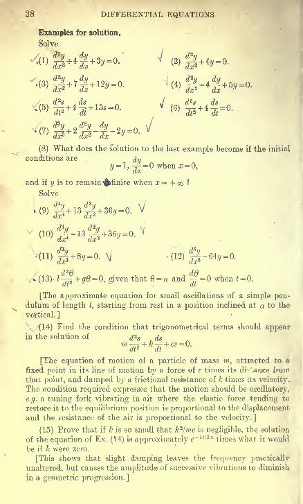
Solve
y,., d2s .ds J d2s . ds _
(7) «^+ 2 &i & 2y_a
(8) What does the solution to the last example become if the initial
conditions are fly
y = l, -p = when x = 0,
and if y is to remain ^finite when x= + co ?
Solve
<»»3-»3 +"»-*- v
t
.
•(H) ^ + 8y=0. \| .(12)g-64<,=0.
,72/3 J/3
* (13) Z-T-g +#0=0, -given that = a and tt=0 when t=0.
[The approximate equation for small oscillations of a simple pen-
dulum of length I, starting from rest in a position inclined at a to the
vertical.]
(14) Find the condition that trigonometrical terms should appear
in the solution of ^2S femdT*
+kdi+cs=0 -
[The equation of motion of a particle of mass m, attracted to afixed point in its line of motion by a force of c times its di -ance from
that point, and damped by a frictional resistance of k times its velocity.
The condition required expresses that the motion should be oscillatory.
e.g. a tuning fork vibrating in air where the elastic force tending to
restore it to the equilibrium position is proportional to the displacement
and the resistance of the air is proportional to the velocity.]
(15) Prove that if k is so small that k 2/mc is negligible, the solution
of the equation of Ex. (14) is approximately e~ kt/2m times what it would
be if k were zero.
[This shows that slight damping leaves the frequency practically
unaltered, but causes the amplitude of successive vibrations to diminish
in a geometric progression. ]
LINEAR EQUATIONS WITH CONSTANT COEFFICIENTS 29
(16) Solve L^ +R^ + Q-O, given that Q=QQ and ^ = when
* = 0, and that CR2 <4:L.
[Q is the charge at time t on one of the coatings of a Leyden jar of
capacity C, whose coatings are connected when t = by a wire of resist-
ance R and coefficient of self-induction L. ]
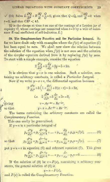
29. The Complementary Function and the Particular Integral. So
far we have dealt only with examples where the f(x) of equation (1)
has been equal to zero. We shall now show the relation between
the solution of the equation when f(x) is not zero and the solution
of the simpler equation derived from it by replacing f(x) by zero.
To start with a simple example, consider the equation
It is obvious that y=x is one solution. Such a solution, con-
taining no arbitrary constants, is called a Particular Integral.
Now if we write y=x+v, the differential equation becomes
2g +R(l.+£) +«t, +.>-5 +*n d%* K dv _ n
'giving v = Ae~2x + Be~ ix,
T so that y=x+Ae-2x +Be-*-x .
The terms containing the arbitrary constants are called the
Complementary Function.
This can easily be generalised.
If y = u is a particular integral of
dny {?n_1
v dy £ . » ia .
*lf+AjSA + ~ +**£ +**-fW (6)
so that Po^a+Pi^=i + -+Pn-i-^.+PnU=f(x), (7)
put y=u + v in equation (6) and subtract equation (7). This gives
dnv dn~xv dv _ /oxV°fan+Pl^+---+Pn-l lx
+PnV=0 (8)
If the solution of (8) be v = F(x), containing n arbitrary con-
stants, the general solution of (6) is
y = u+F(x),
and F(x) is called the Complementary Function.

30 DIFFERENTIAL EQUATIONS
Thus the general solution of a linear differential equation with
constant coefficients is the sum of a Particular Integral and the Com-
plementary Function, the latter being the solution of the equation
obtained by substituting zero for the function of x occurring.
Examples for solution.
Verify that the given functions are particular integrals of the follow-
ing equations, and find the general solutions :
j I *•> p-4+*>-<"- <2 > 3•
-g- i3! +i»
• (3)2sin3a;; j\ + iy = - 10 sin Sx.
For what values of the constants are the given functions particular
integrals of the following equations ? ^
(4)ae»*; g+13^ + 42y»ll2e» ^,>V' X
d 2s \j / d2v- (
5 )aeU
> ij2+9s= QOe
~ t
-&v (6 )
a sin px' ri + y = 12 sin 2cc*
V-^7) a sin px + b cos px ; -=-| + 4 j^ + 3y = 8 cos x - 6 sin x.
<«> •' § +5l +6^ 12 -
Obtain, by trial, particular integrals of the following :
.(11) + 9y = 4Osin5*. <12 > H" 8l + 9!'= 40sill5a; -
»
<
13) § + 8! + 2»30. The operator D and the fundamental laws of algebra. When
a particular integral is not obvious by inspection, it is convenient
to employ certain methods involving the operator D, which stands
for -j-. This operator is also useful in establishing the form of the
complementary function when the auxiliary equation has equal
roots.
d2 d3
D2 will be used for j-2 , D3 for -7-3, and so on.

LINEAR EQUATIONS WITH CONSTANT COEFFICIENTS 31
The expression 2 -y-| + 5 -j- + 2y may then be written
2D*y + 5Dy+2y,
or (2D*+bD + 2)y.
We shall even write this in the factorised form
(2D + l)(D+2)y,
factorising the expression in D as if it were an ordinary algebraic
quantity. Is this justifiable ?
The operations performed in ordinary algebra are based upon
three laws
:
I. The Distributive Law
m(a + b)=ma + mb
;
II. The Commutative Law
ab = ba
;
III. The Index Law am . an =am+n .
Now D satisfies the first and third of these laws, for
D(u+v)=Du+Dv,and Dm . Dnu=Dm+n
. u
(m and n positive integers).
As for the second law, D (cu) = c (Du) is true if c is a constant,
but not if c is a variable.
Also Dm (Dnu) =Dn (Dmu)
(m and n positive integers).
Thus D satisfies the fundamental laws of algebra except in that
it is not commutative with variables. In what follows we shall
write F(D) s p D» +PlD^ + ... +pn_1D +pn ,
where the p's are constants and n is a positive integer. We are
justified in factorising this or performing any other operations
depending on the fundamental laws of algebra. For an example
of how the commutative law for operators ceases to hold when
negative powers of D occur, see Ex. (iii) of Art. 37.
31. F(D)eax =eaxF(a). Since
Deax = aeax,
D2eax =a2eax
,
'
and so on, ,^
F(D) eax = (p Dn +p1
Dn~1 + ... +pn-xI) +pn ) e
ax
^(p^+p^-1 + ... +pn.1a +pn ) eax
=ea*F(a).\

32 DIFFERENTIAL EQUATIONS
32. F(D){eaxV} =eaxF(D +a) V, where V is any function of x. ByLeibniz's theorem for the nth differential coefficient of a product,
D»{eP*V} = (Dneax ) V + w(D"-1eoa') {DV)
+ ln(n-l)(Dn-*eax)(D*V) + ... + eax (DnV)
=ane°*Y +nan-1eazDV +\n{n - l)a»-V*Da7 + ... +eaxDnV=eax (an +nanr1I>k + hn(n - l)an
~2D2 + ...+Dn)V
= ea*(Z)+a)n F.
Similarly Dn~1 {eaxV}=eax(D+a)n-1V, and so on.
Therefore
F(D){eaxV} = (p D» +PlD»~l + ... +pn.1D +pn){e
axV}
= eax{p (D+a)n +p1(D+a)n~1 + ... +pn-x{D +a) +pn}V
= e*xF(D + a)V.
33. F(D 2) cos ax =F( - a 2
) cos ax. Since
D2 cos ax = -a2 cos ax,
Di oosax = (- a2)2 cos ax,
and so on,
F(D2) cos ax = (p D2n +p1D2n~2 + ... +pn-1
D2 +pn) cos ax
= {Po(~ a2)n +Pi(-a2
)
n~1 + ... +pn-i(-«2
) +Pn} cos «#
— F( -a2) cos ax.
Similarly F(D2) sinax=F(-
a
2) sin ax.
34. Complementary Function when the auxiliary equation has equal
roots. When the auxiliary equation has equal roots a and a, it
may be written m2 _ 2ma + a 2 = 0.
The original differential equation will then be
i.e. (D2 -2aZ>+a 2)*/=0,
(D-a) 2y=0 :...(9)
We have already found that y=AeaX is one solution. To find
a more general one put y=e*?V, where V is a function of x.
By Art. 32,
(D -a)*{e?*V} =eaX(D -a +a)2V = (T?D2 V.
Thus equation (9) becomes
D2V=0,
i.e. V =A+Bx,so that y = eax(A+Bx).
m

LINEAR EQL\. X)NSTANT COEFFICIENTS 33
Similarly the equation (D - a)py =
reduces to DPV =0,
giving V = {Ax +A& +A&? + . . . +Ap^'1),
and y = eaX(Ax + A^c +A zx2 + . . . + Ap^xP^x ).
When there are several repeated roots, as in
(D-anD-(3)*(D-yyy =0, (10)
we note that as the operators are commutative we may rewrite the
equation in the form
iD-PnD-yY{{D-aVy}=0,which is therefore satisfied by any solution of the simpler equation
(D- ayy =o'.
(ii)
Similarly equation (10) is satisfied by any solution of
(D-P)*y=0, (12)
or of (D-y)ry=0 (13)
The general solution of (10) is the sum of the general solutions
of (11), (12), and (13), containing together (p+q+r) arbitrary
constants.
Ex. (i). Solve (D*-8D 2 + 16)y = 0, (p.^i.e. (Z)2 -4) 2?/ = 0.
The auxiliary equation is (m 2 -4) 2 = 0,
m = 2 (twice) or -2 (twice).
Thus by the rule the solution is
y = (A + Bx) e2x + (E + Fx) e~2x.
Ex. (ii). Solve (D2 + l) 2*/ = 0.
The auxiliary equation is (m 2 + l) 2 = 0,
m— i (twice) or -i (twice).
Thus y = {A + Bx)eix + {E+Fx)e~ix,
or better y = (P+ Qx) cos x + (R + Sx) sin x.
Examples for solution.
\h) {D* + 2D* + D2)y = 0. >< $) (-D6 + 3Z>* + 32) a + l)y = 0.
^) (Di -2D3 + 2D2 -2D + l)y = 0. $4) (4Z>5 -3Z>3 - D2) t/ = 0. s
(5) Show that
F (D 2){P cosh ax +Q sinh ax) = F(a2)(P cosh ax + Q sinh ax)
.
(6) Show that (D - a)4n
(eax sin px) =p*neax sin px.
35. Symbolical methods of finding the Particular Integral when
f(x) =eax. The following methods are a development of the idea
of treating the operator D as if it were an ordinary algebraic quan-
p.d.e. c

34 DIFE
tity. We shall proceed tentatively, at first performing any opera-
tions that seem plausible, and then, when a result has been obtained
in this manner, verifying it by direct differentiation. We shall use
the notationY7Jy\ /(*)
*° denote a particular integral of the equati„ F(D)y-f{z).
(i) Iff(x) =eax, the result of Art. 31,
F(D) e™ = eaxF (a)
1
"
suggests that, as long as F(a)=j=0, ^y-r eax may be a value ofF(u)
v —v_—"» F(Dy
This suggestion is easily verified, for
W^}-9lSrVyArt.3i.>F(a) J F{a)
= eax .
(ii) If F (a) =0, {D-a) must be a factor of F(D).
Suppose that F(D)=(D -a)p<f>(D), where 0(a)=/=O.
Then the result of Art. 32,
F (D) {eaxV } = eaxF (D + a) V,
suggests that the following may be true, if 7 is 1,
1-^^ 1 _, 1 l(*x .l\ e™ 1 ,/jw*~--. pax j y _F(D) (D-a)P<f>(D) (D-a)p\</>(a){ <j>(a) Dp
e?x xv
adopting the very natural suggestion that jz is the operator inverse
to D, that is the operator that integrates with respect to x, while
y- integrates p times. Again the result obtained in this tentative
manner is easily verified, for
^K^S' byArt - 32 '
= e?x, byArt. 31.

LINEAR EQUATIONS WITH CONSTANT COEFFICIENTS 35
In working numerical examples it will not be necessary to repeat
the verification of our tentative methods.
Ex. (i). (D + 3)2y = 50e*x.
The particular integral ia
(Z> + 3)2 (2+3)
Adding the complementary function, we get
y = 2e2x + {A + Bx)e~3x .
Ex. (ii). (Z>-2) 2i/=.50e2*.
If we substitute 2 for D in jj:—^ 50e2x , we get infinity.
But using the other method,
(D ]_ 2)2• 50e2* = 50e 2ie
-^-2
. 1 = 5Qe2*, \x2 - 25x2e2*. \
Adding the complementary function, we get
y = 25x2e2x + (A + Bx)e2x .
Examples for solution.
Solve v?
m)(D2 + 6D + 25)y=^lQi:^x . rfft) (D2 + 2pD + p2 + q2)y = eax .
:($) (D2 -9)?/ =54^^ m (D3 -D)y = ex + e-x .
(5) (D2 -p2)y = a'2o&px. (6) (D* +iD2 + lD) y = 8e~2x .
36. Particular Integral when f (x) =cos ax. From Art. 33,
(j> (D2) cos ax =
<f> ( - a2) cos ax.
This suggests that we may obtain the particular integral by
writing - a2 for D2 wherever it occurs.
Ex. (i). (D2 + SD + 2) y = cos 2x.
1 1 1. COS 2x = ; t-=: -
. COS 2x = 7rF: rr . cos 2x.D2 + 3D + 2 -4 + 3Z) + 2 3D-2
To get D2 in the denominator, try the effect of writing
1 _ 3Z> + 2
3ZT^2~9Z>2 -4'
suggested by the usual method of dealing with surds.
This gives
—^r—i cos 2x = - xV(3-D cos 2x + 2 cos 2x)- oo - 4
= -t
L .(-6sin2a; + 2cos2a;)
^^(Ssu^aj-cc^a;).

36 DIFFERENTIAL EQUATIONS
Ex. (ii). (Di + 6D2 +nD + 6)y = 2ein3x.
2 sin 3x = 2—^=—
—
:—r-r^—- sin 3xD3 + 6D2 + llD + 6 -9D-54- LD + 6
1
Z)-24
D + 24
Z>2 -576_ i
sin 3z
sin 3x
5 s -(3 cos 3a; + 24 sin Sx)
= - T-^T (cos 3x + 8 sin 3x).
We may now show, by direct differentiation, that the results
obtained are correct.
If this method is applied to
[<f>(D2
) + D\J, (D2) ] y =P cos ax +Q sin ax,
where P, Q and a are constants, we obtain
<j> ( - a2) . (P cos ax +Q sin ax)+a\p- {-a2
) . (P sin ax -Q cos ax)
{^(-a2)}
2 + a2{yjr(-a2)}
2.
It is quite easy to show that this is really a particular integral,
provided that the denominator does not vanish. This exceptional case
is treated later (Art. 38).
Examples for solution.
Solve /
.$& {D + l)y = 10sm2x. fa (Z)2 -5Z) + 6) </ = 100sin ix.
^(3) (Z)2 + 8D + 25)i/ = 48 cos a: -16 sin a.
v<4) (D2 + 2D + 401) y = sin 20z + 40 cos 20x.
(5) Prove that the particular integral of
d2s _ 7ds „
-tt + 2* -t; + V s = a cos atat2 at
may be written in the form b cos (qt - e),
where b = a/{(p 2 -q2)
2 + ik2q2}h and tan € = 2kq/(p2 -q 2
).
Hence prove that if q is a variable and &, p and a constants, 6 is
greatest when q = y/{p2 - 2k2
) = p approx. if k is very small, and then
e = 7r/2 approx. and b = a/2kp approx.
[This differential equation refers to a vibrating system damped
by a force proportional to the velocity and acted upon by an external
periodic force. The particular integral gives the forced vibrations
and the complementary function the free vibrations, which are soon
damped out (see Ex. 15 following Art. 28). The forced vibrations
have the greatest amplitude if the period 2-n-fq of the external force
is very nearly equal to that of the free vibrations (which is

LINEAR EQUATIONS WITH CONSTANT COEFFICIENTS 37
2ir/y/{p2 -k2)=2ir/p approx.), and then e the difference in phase
between the external force and the response is approx. tt/2. This
is the important phenomenon of Resonance, which has important
applications to Acoustics, Engineering and Wireless Telegraphy.]
37. Particular integral when f(x) =xm , where m is a positive integer.
In this case the tentative method is to expand j^ in a series of
ascending powers of D.
Ex.(i). -^^ = 1.(1+^)-^
= i(*2-i).
Hence, adding the complementary function, the solution suggested
for {D*+4)y = z*
is y= \(x2 -^)+A cos 2x4-5 sin 2x.
Ex. (ii).
D2 -iD + S^ =
£ \i^d~3TI)) **> b? Partial fractions,
f / D D2 D3 Z)4 M= i{(l + Z) + Z)2 + Z)3 + Z).4 + ...)- i (l +- +T+- +- + ...)}^
Adding the complementary function, the solution suggested for
(D2 -iD + 3)y = x3
is y^^xS +^ + zg-x +^ + Aet + Be?*.
s*m dhb^T)96x2=w Uwrt x°}
-W.-jTj^-g). from Ex. (i),
-i(S-t)= 2x4 -6x2
.
Hence the solution of D2 (Z)2 + 4) y = 96x2 should be
y = 2x*-6x2 +A cos 2x + Z?sin 2x + E + Fx.
Alternative method.
= (24:D-2 -6 + %D 2 -...)x2
= 2x*-6x 2 + 3.

38 DIFFERENTIAL EQUATIONS
This gives an extra term 3, which is, however, included in the
complementary function.
* The method adopted in Exs. (i) and (ii), where F(D) does not
contain D as a factor, may be justified as follows. Suppose the expan-
sions have been obtained by ordinary long division. This is always
possible, although the use of partial fractions may be more convenient
in practice. If the division is continued until the quotient contains Dm,
the remainder will have Dm+1 as a factor. Call it <p(D) . Dm+1. Then
^= CQ+ c1D + c2D* + ...+cmn™ + *iD]}-
]̂
+1
(1)
This is an algebraical identity, leading to
l = F(D){c + c1D + ctD* + ...+cmDm} + <f>{D) . D"*1
(2)
Now equation (2), which is true when D is an algebraical quantity,
is of the simple form depending only on the elementary laws of algebra,
which have beffc shown to apply to the operator D, and it does not
involve the difficulties which arise when division by functions of D is
concerned. Therefore equation (2) is also true when each side of the
equation is regarded as an operator. Operating on xm we get, since
Dm+1xm = 0,
xm =F(D){{c(t+ c1
D + c2D2 + ...+cmDm)xm}, (3)
which proves that the expansion obtained in (1), disregarding the
remainder, supplies a particular integral of F(D)y=xm .
It is interesting to note that this method holds good even if the
expansion would be divergent for algebraical values of D.
To verify the first method in cases like Ex. (iii), we have to prove
that 1
i.e. (c D-r + c1D~r+1 + c 2D-
r+2 + ... +cmD~r+m
) xm,
is a particular integral of {F(D) . Dr}y = xm,
i.e. that {F(D) . Dr} {(cQD-
r +c^*1 + c2D~r+2
+ ...+cmD-r+m)xm}=xm (4)
Now {F( D) . D'} u m F(D) . {Dru},
also Dr{(c8D ~ '+*) xm} = (cgD*) xm
;
hence the expression on the left-hand side of (4) becomes
F(D){(c + c1D + c2D* + ...+cmD™)xm} = x'», by (3),
which is what was to be proved.
In the alternative method we get r extra terms in the particular
integral, say(Cffi+1Z)^^+...+W2>»)*«
These give terms involving the (r-l)th and lower powers of x.
But these all occur in the complementary function. Hence the first
method is preferable.
* The rest of this article should be omitted on a first reading.
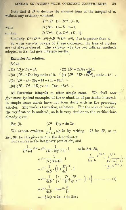
LINEAR EQUATIONS WITH CONSTANT COEFFICIENTS 39
Note that if D~hi denotes the simplest form of the integral of u,
without any arbitrary constant,
D-1(DA) = D-1. 0=0,
while i>{2H.l)-X>.*-l,
so that D(D-1 .l)^D-1 .(Z).l).
Similarly Dm (D-m . xn)=^D-m(Dm . xn ), if m is greater than n.
So when negative powers of D are concerned, the laws of algebra
are not always obeyed. This explains why the two different methods
adopted in Ex. (iii) give different results.
Examples for solution.
Solve
-j(l) (D + \)y = %*. /(2) (D2 + 2D)y = 2ix.
^(3) (D2 -6D + 9)y = 5±x + l8. ' (4) (D4 -6D3 + 952)?/ = 54a: + 18. ,
v/(5) (D2 -D-2)y =U-76x-±8x2.
JG) (IP-D2 -2D)y =U-76x-±8x2. U
38. Particular integrals in other simple cases. We shall now
give some typical examples of the evaluation of particular integrals
in simple cases which have not been dealt with in the preceding
articles. The work is tentative, as before. For the sake of brevity,
the verification is omitted, as it is very similar to the verifications
already given.
Ex. (i). (D2 + 4)y=sm2x.
We cannot evaluate -^—j sin 2x by writing - 2 2 for D2, as in
Art. 36, for this gives zero in the denominator.
But i sin 2x is the imaginary part of e2ix, and
eax = e2ix t if
as m Art. 35,Z)2 + 4 (Z> + 2*') 2 + 4
— x _ JLL_.i ±-S*> -x.i
1 I. Dv* c a".
-'"OT-{(»-B+™--)-U P)
" e4*D 4*
« - |«x(cos 2a; + 1 sin 2x)
;
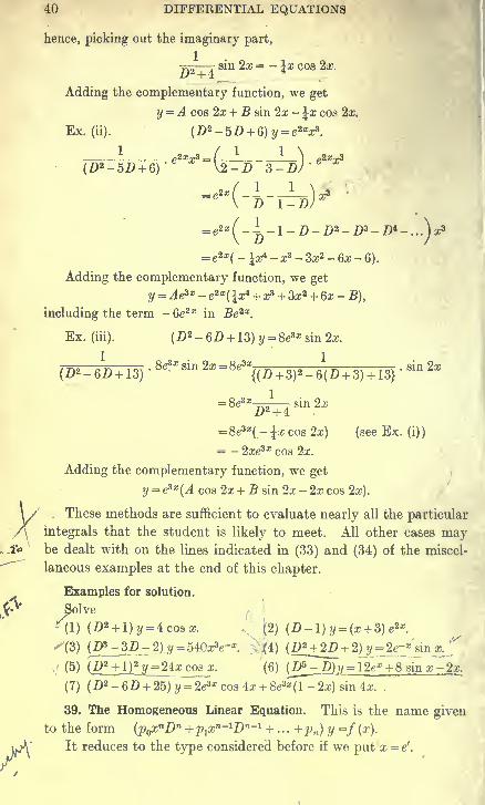
40 DIFFERENTIAL EQUATIONS
hence, picking out the imaginary part,
™—r sin 2x = - \x cos 2x.
Adding the complementary function, we get
y =A cos 2x + B sin 2x - \x cos 2x.
Ex. (ii). (D2 - 52) + 6) y = e2xx*.
(D2-5D + 6) \2-D 3-D/ ^
= e2x(4-r^)^*
= e2* (- ^ - 1 - D - D2 - D3 - D* - ...) a?
= e2*( - \x* - x3 - 3x2 - 6x - 6).
Adding the complementary function, we get
y = A<?x - e**{\x* + x3 + 3x* + 6x- B),
including the term - 6e2x in Be2x.
Ex. (iii). (Z)2 - 6D + 13) y = 8<?x sin 2x.
. 8<?x sin 2x = 8eSx,,„ ..,„ * -^—r^ . sin 2x(D 2 -6D + 13)" {(D + 3)
2 -6(Z) + 3) + 13}
= 8e3a:-K5—7sin2z
= 8e3a:( - \x cos 2x) (see Ex. (i)
)
= - 2xe?x cos 2x.
Adding the complementary function, we get
y = e?x (A cos 2x + B sin 2x - 2x cos 2x).
These methods are sufficient to evaluate nearly all the particular
integrals that the student is likely to meet. All other cases maybe dealt with on the lines indicated in (33) and (34) of the miscel-
laneous examples at the end of this chapter.
Examples for solution.
Solve
"(1) (Z)2 + l)</ = 4cosa;. (2) (D-l) y = (x + 3) e*x .
y\Z) (D!i -3LD-2)y = 5i0x3e-x . y(i) (DM-2D + 2) y»2e-*«n x. f:
(5) {D^+}J^ji=2ixcosx. (6) (W^~D)y = \2ex + 8 sin x -2x.
(7) (D2 -6D + 25)y = 2e3*cos4:r + 8e3a:(l-2:r)sin4x. .
39. The Homogeneous Linear Equation. This is the name given
to the form {p(fcnBn +p1
xn~1Dn-1 + . . . +pn ) y =f (x).
It reduces to the type considered before if we put x = e'.

LINEAR EQUATIONS WITH CONSTANT COEFFICIENTS 41
Ex. (x3D3 + 3x2D2 + xD)y = 2ix2.
Put x = el
,
dx_t _
dt~6=X>
t. _. d dt d 1 d
so that D =dZ=" d
-x jr-Jt
'
\xdt) x*dt+x dt x2 \ dt^dt2).'
x2 \ dt+
dt 2) a*\ dt+
dt 2J+x2 \ dt
+dt2/
x*\ dt+
dt 2)+x3 \ dt 2
+dt?)
x*\ dt dt2 dtV'd u
thus the given differential equation reduces to -^ = 2ie2
\
giving y = A + Bt + Ct2 + 3eit
= A + B\ogx + C(logx) 2 + 3x 2.
Another method is indicated in (28)-(30) of the miscellaneous
examples at the end of this chapter.
The equation
p (a+bx)nDny +p1 (a + bx)n-1Dn~1y + ... +pny =f(x)
can be reduced to the homogeneous linear form by putting
z = a +bx, giving^ = dy^dydz =b
dyy dx dz dx dz
'
Examples for solution.
/(I) x2^-2x d£ + 2y =M. / (2) ^g + 9x| + 25^50.
(3) x3^ + 3:K2§ + a;| + 8^= 65c0s(l0^)
-
W ^dx*+ Z
^dx*+ X
dx 2Xdx
+ y ~ [°gX -
(5) (1+2^2-6(1 +2x)g + 16^r8 (l+2a:)«.
(6) (l + x)2<^ + (l+x)
d£ + y==ico8log(l+x).

42 DIFFERENTIAL EQUATIONS
40. Simultaneous linear equations with constant coefficients. The
method will be illustrated by an example. We have two de-
pendent variables, y and z, and one independent variable x.
D stands for -»-, as before.ax
Consider (52)+4) y -(2D + l)z = e~x , (1)
(D + S)y- 3z =be~x (2)
Eliminate z, as in simultaneous linear equations of elementary
algebra. To do this we multiply equation (1) by 3 and operate on
-equation (2) by (22) + 1).
Subtracting the results, we get
{3 (52) +4) - (22) + 1)(D + 8)} y = Se~x - (2D + 1) 5e~*,
i.e. (-2D2 -2D + ±)y = Ser*t
or (D2jD-2)y = -4<r*
Solving this in the usual way, we get
y = 2e-x +Aex +Be~2x.
The easiest way to get z in this particular example is to use
•equation (2), which does not involve any differential coefficients of z.
Substituting for y in (2), we get
Ue~x + 9Aex + QBe~2x - 3z = 5e~*,
so that z = 36-* + 3Aex + 2Be~2x.
However, when the equations do not permit of such a simple
method of finding z, we may eliminate y.
In our case this gives
{ - (2) +8) (2D + 1) + 3(52) + 4)} y = {D + S)e~x - (52) + 4)5e"*,
i.e. (-22)2 -22) + 4)z = 12e-*,
-giving z = 3e~x + Eex + Fe~2x.
To find the relation between the four constants A, B, E, and F,
substitute in either of the original equations, say (2). This gives
(2) + 8) (2e~x + Aex + Be~2x
)- 3 {3e~x + Eex + Fe~2x
) = 5e~x,
i.e. (9A - ZE) ex + (6# - 32?) e~2x = 0,
whence E = ?>A and F = 2B,
so z = Se~x + Eex + Fe~2x = 3e~x + 3^e* + 2Be~2x, as before.
Examples for solution.
(1) Dy-z = 0, (2) (Z>- 17) t/ + (22)- 8)2 = 0,
(D-l)y-(D + \)z = 0.,
(132)- 53)?/- 22 = 0.
<3) (22)2 -2) + 9)y-(Z)2 + 2) + 3)2 = )
(22)2 + D + 7) y -{D 2-D + 5)2=0.

LINEAR EQUATIONS WITH CONSTANT COEFFICIENTS 43
<4) (D + \)y = z + ex, (5) {D2 + b)y-d = -36cos 7x,
{D + l)z = y + ex . p>n)2z = 99co8 7x.
(6) (2.D + l)«/ + (Z> + 32)z = 91e-* + 147sin2a; + 135cos2a;,
y-(D-8)z = 29e~x + 47 sin 2x + 23 cos 2x.
MISCELLANEOUS EXAMPLES ON CHAPTER III.
Solve
/O) (Z)-l)32/ = 16e3*. (2) (4D2 + 12Z) + 9)i/ = 144a*fH
u <3) (D* + 6IP + nD2 + 6D) y = 20e~2x sin x.
<4) (D3-D2 + 4:D-i)y = 68ex am2x.
(5) (D*-6D2 -8D-S)y = 256(x + l)(?x .
(6) (ZH-8Z)2 -9)i/ = 50sinh2a;. (7) (Z>»-2Z) 2 + 1) */ = 40cosh x.
(8) (Z)-2) 22/ = 8(x2 + e2* + sin2x). (9) (D-2) 2y = 8x2e2x Bin 2x.
<10) (7)2 + l)?/ = 3cos 2a; + 2 8in3 x.
<11) (D* + lOD2 + 9)y = 96am2xcosx.
(12) (D-a)ay = ax, where a is a positive integer.
ax2 x ax x2 dx2 x dx
<15 > % =f ^ (, + l) 2g + (, + l)gH2x + 3)(2x + 4).
§ +4§ + 4, = 25* + W.
«**-* £-*;>* <l«)£ + I-0; <§+ *-0.
(21) Show that the solution of (D2n+1 -l)y = consists of Je* andn pairs of terms of the form
efx (Br cos sx + Cr sin sx),
. 2ttt . . 2xrwhere c= cos ^ and s = sin -
,
2w +
1
2n +
1
r taking the values 1, 2, 3 ... n successively.
(22) If (D-a)u = 0,
(D-a) v = u,
and (D- a)y = v,
find successively w, w, and y, and hence solve (D-a)3</ =
/

44 DIFFERENTIAL EQUATIONS
(23) Show that the solution of
(D-a)(D-a-h)(D-a-2h)y=0
can be written Aeax + B^x -—r—-+Ceax - ^ '-.
h h*
Hence deduce the solution of (D- a)zy = 0.
[This method is due to D'Alembert. The advanced student will
notice that it is not quite satisfactory without further discussion. It
is obvious that the second differential equation is the limit of the first,
but it is not obvious that the solution of the second is the limit of the
solution of the first.]
oz o z
(24) If {D-a)3emx is denoted by z, prove that z, =— , and =—^ all
vanish when m = a.
Hence prove that eax , xe?x
, and x2eax are all solutions of (D - a)3y =0.
[Note that the operators {D-af and -~— are commutative.]
.-„, .., , ,cos ax - cos (a + h) x
(25 Show that ; ,. 2
v.
x(a + h) 2 -a 2
is a solution of (D2 + a 2) y = cos (a + h) x.
Hence deduce the Particular Integral of (D2 + a2)y = cos ax.
[This is open to the same objection as Example 23.]
(26) Prove that if V is a function of x and F(D) has its usual
meaning,
(i) Dn [xV] =xDnV + nDn-W\(ii) F(D)[xV] = xF{D)V + F'(D)V;
(iii)^-rsri-s— 7-F{D)
v-{m}F(D) [
-J F(D)
V[F(D)] 2
'
(iv) <p(D)[xnV] = xntp{D)V + nxn-1</>'(D)V + --- + nC,.xn-r
<f>
r(D)V
where <p{D) stands for •
(27) Obtain the Particular Integrals of (i) (D- l)y = xe2x,
(ii) (D + l)y = x2 coax,
by using the results (iii) and (iv) of the last example.
(28) Prove, by induction or otherwise, that if 6 stands for x 3-,
x»^=e(d-l)(0-2)...(0-n + l)y.
(29) Prove that
(i) F(6)xm = xmF{m);
xm(u) jrgf ~r$sj- provided F (m)±°'-
(iii» m [xmV]=
^-FW^) v-
where V is a function of x.

LINEAR EQUATIONS WITH CONSTANT COEFFICIENTS 45
(30) By using the results of the last question, prove that the solu-
tion ofd2 d ..-,-. „ „x2j\-ix~+%y = x5 is $x5 + Axa + Bxb
,
-where a and b are the roots of m{m - 1) - 4m + 6 = 0,
i.e. 2 and 3.
(31) Given that (D-l)y = e2x,
prove that (D-l)(D-2)y = 0.
By writing down the general solution of the second differential
equation (involving two unknown constants) and substituting in thefirst, obtain the value of one of these constants, hence obtaining the
solution of the first equation.
d2y
(32) Solve j 2̂ +p2y = sin ax by the method of the last question.
(33) If u x denotes eax I ue~ax dx,
u 2 denotes ebx
I u^er** dx,
etc.,
prove the solution of F(D)y = u, where F(D) is the product of nfactors.
(D-a)(D-b)...
may be written y = un-
This is true even if the factors of F(D) are not all different.
Hence solve (D-a)(D-b)y = eax log x.
(34) By putting „ ~ into partial fractions, prove the solution of
F(D)y = u may be expressed in the form
2-^rrreaa;l ue~
ax dx,F'{a) J
provided the factors of F(D) are all different.
[If the factors of F(D) are not all different, we get repeated inte-
grations.]
Theoretically the methods of this example and the last enable us to
solve any linear equation with constant coefficients. Unfortunately,
unless u is one of the simple functions (products of exponentials, sines
and cosines, and polynomials) discussed in the text, we are generally
left with an indefinite integration which cannot be performed.
If u =f(x), we can rewrite eax I ue~ax dx
in the form f(t)ea ^-^dt,
where the lower limit Jc is an arbitrary constant.

46 DIFFERENTIAL EQUATIONS
(35) (i) Verify that
1 f
*
y = ~\ f(t)ainp(x-t)dt
is a Particular Integral of
[Remember that if a and b are functions of x,
(ii) Obtain this Particular Integral by using the result of the last
example.
(iii) Hence solve (Z) 2 + l)i/ = cosec x.
(iv) Show that this method will also give the solution of
(in a form free from signs of integration), if f(x) is any one of the func-tions tan x, cot x, sec x).
(36) Show that the Particular Integral of j~ + p 2y = k cos pt repre-
sents an oscillation with an indefinitely increasing amplitude.
[This is the phenomenon of Resonance, which we have mentionedbefore (see Ex. 5 following Art. 36). Of course the physical equatic
of this type are only approximate, so it must not be assumed thatjpie
oscillation really becomes infinite. Still it may become too^pgefor safety. It is for this reason that soldiers break step on c^£hg abridge, in case their steps might be in tune with the natural osOTlation
of the structure. ]
(37) Show that the Particular Integral of
-^ + 2h-^ + (h 2 + p 2)y = Jce-
ht cospi
krepresents an oscillation with a variable amplitude —te~ ht
.
Find the maximum value of this amplitude, and show that it is verylarge if h is very small. What is the value of the amplitude after aninfinite time ?
[This represents the forced vibration of a system which is in reson-
ance with the forcing agency, when both are damped by friction. Theresult shows that if this friction is small the forced vibrations soonbecome large, though not infinite as in the last example. This is anadvantage in some cases. If the receiving instruments of wireless
telegraphy were not in resonance with the Hertzian waves, the effects
would be too faint to be detected.]

LINEAR EQUATIONS WITH CONSTANT COEFFICIENTS 47
(38) Solve ^~ n*y=0 -
[This equation gives the lateral displacement y of any portion of athin vertical shaft in rapid rotation, x being the vertical height of theportion considered. ]
(39) If, in the last example,
-i =y=0 when x=0 and x = l,
prove that y = E(coa nx - cosh nx) + F(ain nx - sinh nx)
and cos nl cosh nl = 1
.
[This means that the shaft is supported at two points, one a height
I above the other, and is compelled to be vertical at these points. Thelast equation gives n when I is known.]
(40) Prove that the Complementary Function of
becomes negligible when t increases sufficiently, while that of
dzy d 2y _
oscillates with indefinitely increasing amplitude.
[An equation of this type holds approximately for the angularvelocity of the governor of a steam turbine. The first equation corre-
sponds to a stable motion of revolution, the second to unstable motionor " hdyting." See the Appendix to Perry's Steam Engine.
]
(41) fSgove that the general solution of the simultaneous equations :
m d£=Ve-He dJ,dt 2 dt
mdt*~
Medt'
where m, V, H, and e are constants, is
x =A + B cos {at - a),
Vy == t + C + B sin ( cot - a),
Hewhere w =— and A, B, C, a are arbitrary constants.
Given that — = -^ = x =y=0 when t = 0, show that these reduce to
x=—-(1 -COS tot),ton.
V .
y= —jj (cot - sin tot), the equations of a cycloid.

48 DIFFERENTIAL EQUATIONS
[These equations give the path of a corpuscle of mass m and charge
e repelled from a negatively-charged sheet of zinc illuminated with
ultra-violet light, under a magnetic field H parallel to the surface. V is
the electric intensity due to the charged surface. By finding ex-
perimentally the greatest value of x, Sir J. J. Thomson determined
IV m—=, from which the important ratio — is calculated when V and H are<*>H e
known. See Phil. Mag. Vol. 48, p. 547, 1899.]
(42) Given the simultaneous equations,
- (1*11 ..dH* I
x „
.(1*1
'^(Z 2/, I 2
where Lv L2 , M, cv c2 , E and p are constants, prove that I
xis of the
form a x cos pt +A x cos (mt -a) + B1 cos (nt - /3),
and 1 2 of the form
a2 cos pt + A 2 cos (mt -a) + B2 cos (nt - /3),
Ewhere a
i = TFa(l -P 2c2L 2)>
EM3
<X 2— , p C]C 2 ,
k denoting the expression
(LXL 2
-M 2) cxc2^ - (LlCl +L 2c2)p
2 + 1 ;
m and n are certain definite constants ; A 1} Bv a and /3 are arbitrary
constants ; and A 2 is expressible in terms of A xand B2 in terms
of A 2 .
Prove further that m and n are real if Lv L2 , M, cv and c2 are real
and positive.
[These equations give the primary and secondary currents Ixand
7 2in a transformer when the circuits contain condensers of capacities
Cj and c2 . Lxand L 2
are the coefficients of self-induction and M that
of mutual induction. The resistances (which are usually very small)
have been neglected. E sin pt is the impressed E.M.F. of the primary.]

CHAPTER IV
SIMPLE PARTIAL DIFFERENTIAL EQUATIONS
41. In this chapter we shall consider some of the ways in which
partial differential equations arise, the construction of simple par-
ticular solutions, and the formation of more complex solutions from
infinite series of the particular solutions. We shall also explain the
application of Fourier's Series, by which we can make these complex
solutions satisfy given conditions.
The equations considered include those that occur in problems
on the conduction of heat, the vibrations of strings, electrostatics
and gravitation, telephones, electro-magnetic waves, and the
diffusion of solvents.
The methods of this chapter are chiefly due to Euler, D'Alembert,
and Lagrange.*
42. Elimination of arbitrary functions. In Chapter I. we showed
how to form ordinary differential equations by the elimination of
arbitrary constants. Partial differential equations can often be
formed by the elimination of arbitrary functions.
Ex. (i). Eliminate the arbitrary functions /and F from
y=f(x-«l) + F(x + at) (!)
We get ^ =f\x - at) + F'(x + at) •
and<
^=f"(x-al) + F"(x + at) (2)
Similarly -~ — - af'(x - at) + aF'(x + at)
and yi = a 2f"{x-at)+a 2F"(x + at) (3)
* Joseph Louis Lagrange of Turin (1730-1813), the greatest mathematician of
the eighteenth century, contributed largely to every branch of Mathematics. Hecreated the Calculus of Variations and much of" the subject of Partial Differential
Equations, and he greatly developed Theoretical Mechanics and Inlinitesimal
Calculus.
p.d.b. 49 u
C*o

50 DIFFERENTIAL EQUATIONS
From (2) and (3), g =Ig : (4)
a partial differential equation of the second order.*
Ex. (ii). Eliminate the arbitrary function / from
-/©
dz dz nso sc^+w^ =0.
dx * By
Examples for solution.
/ Eliminate the arbitrary functions from the following equations :
y (1) z=f(x + ay). /(2) z=f(x + iy) + F(x-iy),wheTei*=-l.
v/ (3) z =f (x cos a + y sin a - at) + F(x cos a + y sin a + at).
/(4) z=f(x 2 -y 2). v (5) z = e
ax+bvf(ax-by).
- (6) -*/©•
43. Elimination of arbitrary constants. We have seen in
Chapter I. how to eliminate arbitrary constants by ordinary
differential equations. This can also be effected by partials.
Ex. (i). Eliminate A and p from z = Aeptsin px.
d 2z— = - p2Ae pt sin px,
d 2z
2 = p2Ae pt sin px ;
d!
dx2+
dt 2
Eliminate a, b, and c from
z = a(x + y) + b(x-y) +abt + c.
dzWe get =-=a + b,
dz7— =a-b,
ay
dz ,=-=00.dt
* Tin's equation holds for the transverse vibrations of a stretched string.
The most general solution of it is equation (1), which represents two wavestravelling with spied a, one to the right and the other to the left.
PARTIAL DIFFERENTIAL EQUATIONS 51
But (a + o) 2 -(a-&) 2 = 4a&.
(!)'-(!)'-£•
Examples for solution.
Eliminate the arbitrary constants from the following equations :
<i(l) z= Ae-P2t cos px. */(2) z = Ae-?1 cos qx sin ry, where p2 = q
2 + rl.
y/{Z) z = ax + (\-a)y + b. (4) z = ax + by + a2 + b2 .
'(5) 2 = (x-a) 2 + (t/-6) 2. (6) az + b = a2x + y.
44. Special difficulties of partial differential equations. As we have
already stated in Chapter I., every ordinary differential equation
of the nth order may be regarded as derived from a solution con-
taining n arbitrary constants* It might be supposed that every
partial differential equation of the nth order was similarly derivable
from a solution containing n arbitrary functions. However, this is
not true. In general it is impossible to express the eliminant of
n arbitrary functions as a partial differential equation of order n.
An equation of a higher order is required, and the result is not
unique."!*
In this chapter we shall content ourselves with finding particular
solutions. By means of these we can solve such problems as most
commonly arise from physical considerations. J We may console
ourselves for our inability to find the most general solutions by the
reflection that in those cases when they have been found it is often
extremely difficult to apply them to any particular problem. §
It will be shown later (Chap. VI.) that in certain exceptional cases anordinary differential equation admits of Singular Solutions in addition to thesolution with arbitrary constants. These Singular Solutions are not derivablefrom the ordinary solution by giving the constants particular values, but are of
quite a different form.
tSee Edwards' Differential Calculus, Arts. 512 and 513, or Williamson'sDifferential Calculus, Art. 317.
X The physicist will take it as obvious that every such problem has a solution,
and moreover that this solution is unique. From the point of view of puremathematics, it is a matter of great difficulty to prove the first of these facts
:
this proof has only been given quite recently by the aid of the Theory of IntegralEquations (see Heywood and Frechet's L'Equation de Fredholm et ses application.?
a la Physique Math6matique). The second fact is easily proved by the aid of
Green's Theorem (see Carslaw's Fourier's Series and Integrals, p. 206).
§For example, Whittaker has proved that the most general solution of
Laplace's equation twit t&v 7VV
3a;2 dy2 3z2 ~
V= I f(x cos t + y sin t + iz, t) dt,
but if we wish to find a solution satisfying certain given conditions on a givensurface, we generally use a solution in the form of an infinite series.

52 DIFFERENTIAL EQUATIONS
45. Simple particular solutions.
d 2z 1 dzEx. (i). Consider the equation ,-
2=-
2r (which gives the con-
duction" of heat in one dimension). This equation is linear. Now, in
the treatment of ordinary linear equations we found exponentials very
useful. This suggests z = e"u:+nt as a trial solution. Substituting in
the differential equation, we get
a2 *
which is true if n=m 2a2.
ThUs e""'+"l2a2<
is a solution.
Changing the sign of m, e'mx+nfiaH
is also a solution.
Ex. (ii). Find a solution of the same equation that vanishes when
t= +oo .
In the previous solutions t occurs in ew2a2t
. This increases with t,
since m 2a 2is positive if m and a are real. To make it decrease, put
m = ip, so that m 2a 2 = - p2a2
.
This gives eipx ~ p2aH as a solution.
Similarly e-^ -^"2
' is a solution.
Hence, as the differential equation is linear, e~ p2a2t(Aeipx + Be~ ipx) is
a solution, which we replace, as usual, by
e~ p'
kl\E cos px + F sin px).
d 2z d 2zEx. (iii). Find a solution of ^-^ + ^~^=^ which shall vanish when
y = + oo , and also when x = 0. ^
Putting z = emx+ny , we get (m 2 + n2)emx+nv = 0, so m 2 + n 2 =0.
The condition when y = + oo demands that n should be real and
negative, say n= -p.
Then m = ± ip.
Hence e~vy{Aeipx + Be~ipx) is a solution,
i.e. e~vi'(E cos px.-\- F sm px) is a solution.
But z = if x = 0, so E = 0.
The solution required is therefore Fe~P!/ sin px.
Examples for solution.
O^U u it
(1) ~-| = =-£-, given that y = when x = + oo and also when t = + oo .
d 2z 1 9 2z(2) —- =-x =-j, given that z is never infinite (for any real values ofv ox 2 a 2 oy 2
x or y), and that 2=0 when x = or y = 0.
(3) \-a „-=0, given that z is never infinite, and that =- =0 whenK
' dx dys ox
x=*y=>(X

PARTIAL DIFFERENTIAL EQUATIONS 53
d 2V d 2V d 2 V(4) 5
, 2 +2_ 2 + "^T=: ^' giyen that V=0 when z=+oo, when
y= - oo , and also when 2 = 0.
(5) p-g = - - , given that V is never infinite, and that V = C and
dV dV dV . ,
x—•»-=-= -5-= when x = y = z=0.ox ay oz
d 2V d 2V dV(6) -2^" + "2~i
=ar> given that V =0 when £ = + oo
, when x=0 or
I, and when ?/ = or I.
46. More complicated initial and boundary conditions.* In Ex. (iii)
of Art. 45, we found Fe~py sin fx as a solution of
dx2+
dy2 ~ '
satisfying the conditions that z=0 if y= + oo or if £=0.
Suppose that we impose two extra conditions,"}- say 2=0 if x = l
and 2 = Ix - x2if «/ =0 for all values of x between and I.
The first condition gives sin pi =0,
i.e. pi = nw, where n is any integer.
For simplicity we will at first take I = w, giving p = n, any integer.
The second condition gives F sin px = irx- x2 for all values of x
between and ir. This is impossible.
However, instead of the solution consisting of a single term, we
may take
Fxe~y sin x +F2e~
2y sin 2x +F3e-3y sin 3x + . . . ,
since the equation is linear (if this is not clear, cf. Chap. TIL Art. 25),
giving p the values 1, 2, 3. ... and adding the results.
By putting y = and equating to irx - x2 we get
FAsin x +F2 sin 2x +F3 sin 3x + . .
.
= ttx-x2 for all values of & between and tr.
The student will possibly think this equation as impossible to
satisfy as the other, but it is a remarkable fact that we can choose
values of the F's that make this true.
This is a particular case of a more general theorem, which we
now enunciate.
* As t usually denotes time and x and y rectangular coordinates, a condition
such as z = when t = is called an initial condition, while one such as z= if
a;= 0, or if x = l, or if y= x, is called a boundary condition.
fThis is the problem of finding the steady distribution of temperature in a
semi-infinite rectangular strip of metal of breadth I, when the infinite sides are
kept at 0° and the base at (Ix - x2)°.

54 DIFFERENTIAL EQUATIONS
47. Fourier's Half-Range Series. Every function of x which
satisfies certain conditions can be expanded in a convergent series
of the form
/ (x) = a1 sin x + a2 sin 2x + a3 sin 3x + . . . to inf.
for all values of x between and -k (but not necessarily for the
extreme values x=0 and x = ir).
This is called Fourier's * half-range sine series.
The conditions alluded to are satisfied in practically every
physical problem."]"
Similarly, under the same conditions f(x) may be expanded in
a half-range cosine series
l + Zx cos x +
1
2 cos 2x +
1
3 cos 3x + .
.
. to inf.
These are called half-range series as against the series valid
between and 2ir, which contains both sine and cosine terms.
The proofs of these theorems are very long and difficult. J How-
ever, if it be assumed that these expansions are possible, it is easy to
find the values of the coefficients.
Multiply the sine series by sin nx, and integrate term by term, §
giving
pir PIT rn
I f(x)smnxdx = a1 \ sin x sin nx dx + a2 1 sin 2x sin nxdx + ... .
Jo Jo Jo
The term with an as a factor is
sin2 nx dxan I si]
Jo
a r 1 •~\ n
(1 -cos 2nx)dx = ~ x - „ sin 2nx\2 L 2/i Jo2 Jo
= ^an7r.
* Jean Baptiste Joseph Fourier of Auxerre (1768-1830) is best known as theauthor of La Th4orie analytique de la chaleur. His series arose in the solution of
problems on the conduction of heat.
f It is sufficient forf(x) to be single-valued, finite, and continuous, and haveonly a limited number of maxima and minima between sc= and x= w. However,these conditions are not necessary. The necessary and sufficient set of conditions
has not yet been discovered.
X For a full discussion of Fourier's Series, see Carslaw's Fourier's Series andIntegrals and Hobson's Theory of Functions.
§ The assumption that this is legitimate is another point that requires
justification.

PARTIAL DIFFERENTIAL EQUATIONS 65
The term involving any other coefficient, say ar , is
ar sin rx sin nx dx
= -~\ {cos (n - r)x- cos (n+r)x}dx
^ar rsia(n -r)x sin (n+r)x~y
2l n-r n + r J=
'
So all the terms on the right vanish except one.
Thus I f(x) sin nx dx = \an ir,
2 f /.,01 an = -\ f(%) sin nx dx.
Similarly, it is easy to prove that if
f(x) =b + b1 cos x + 62 cos 2o3 + . .
.
for values of a; between and tt, then
1 rttJo
and bn = /(«) cos wee (Zx
for values of n other than 0.
48. Examples of Fourier's Series.
(i) Expand ttx-x 2 in a half-range sine series, valid between x=and x = 7r.
It is better not to quote the formula established in the last article.
Let 7rx - x 2 = a1 sin x + a 2 sin 2x + a 3 sin 3x + . . . .
Multiply by sin nx and integrate from to tt, giving
I (7rx - x2) sin nx dx = an \ sin 2 nxdx = ~ an , as before.
Now, integrating by parts,
I (irx-x 2) sin nxdx =
\
— {ttx - x 2) cos nx\ +- (tt - 2x) cos nx dx
Jo L n J wj v
= + —= (x - 2x) sin wz + —~\ sin wa; tZirU 2Jo ™ 2
Jo
2 r t 4 .= —5 cos nx =— if n is odd or if « is even.w L Jo n
o
Thus an =—g if w is odd or if w is even, giving finally
ttx - x 2 = - (sin cc + -gV sin 3x + T I T sin 5x + . ..).
7T

56 DIFFERENTIAL EQUATIONS
(ii) Expand /(as) in a half-range series valid from x =0 to x = ir, where
f{x) — mx between x — and x = —Z
and f(x) = m{7r-x) between x = — and sc= 7r.
In this case f(x) is given by different analytical expressions in
different parts of the range.* The only novelty lies in the evaluation
of the integrals.
In this case
1 f(x) sin nx dx= I f(x) sin nx dx+\ f(x) sin wx cZx
Jo Jo J|7T
= I mx sin nx dx + I m(7r - x) sin wx dx.
Jo J|
We leave the rest of the work to the student. The result is
d-fyy— (sin z-^sin Sx + r̂ sin So;-^ 8* 11 7as+ ...).
The student should draw the graph of the given function, andcompare it with the graph of the first term and of the sum of the first
two terms of this expansion. f
Examples for solution.
Expand the following functions in half-range sine series, valid
between x= and x = tt :
(1) 1. (2) x. (3) Xs . (4) cos a. (5) ex.
(6) f(x)=0 from x=0 to x=—, and from x=— to tt,
f(x) = (4:X-7r)(37r-4:x) from x = — to x=-r-.
(7) Which of these expansions hold good (a) for x — ?
(6) for x — 7t ?
49. Application of Fourier's series to satisfy boundary conditions.
We can now complete the solution of the problem of Art. 46.
We found in Art. 46 that
Fxe-v sin x+F2e~
2" sin 2x +_F3e~3 " sin 3a; + ...
satisfied all the conditions, if
Fx sin x +F2 sin 2x +F3 sin Sx + . . . = irx - x2
for all values of x between and 7r.
* Fourier's theorem applies even if f(x) is given by a graph with no analyticalexpression at all, if the conditions given in the footnote to Art. 47 are satisfied.
For a function given graphically, these integrals are determined by arith-metical approximation or by an instrument known as a Harmonic Analyser.
t Several of the graphs will be found in Carslaw's Fonrur's Series mid Inter/rah,Art. 59. More elaborate ones are given in the Phil. May., Vol. 45 (1898).

PARTIAL DIFFERENTIAL EQUATIONS 57
In Ex. (i) of Art. 48 we found that, between and -k,
o
r- (sin x + -jV sm 3a; + y^T sin 5a; + ...) = ttx - a;2.
7T
Thus the solution required is
- {e~'J sin a; + T̂ e~Z!l sin 3a; + 1-J--5
e~5j/ sin 5a; + . . .).
7T
50. In the case when the boundary condition involved I instead
of ir, we found Fe~vy sin jpx as a solution of the differential equation,
and the conditions showed that p, instead of being a positive integer
n, must be of the form mr/l.
Thus F^e-^' sin ttx/1 +F2e~in^1 sin 2 irx/l + . .
.
satisfies all the conditions if
Ft sin 7rx{l +F2 sin Sirx/l + ...=lx-x2
for all values of x between and I.
I2
I2
Put ttx/1 = z. Then Ix -x2 = —-A-kz-z2). The F's are thus -=
7T 7T
times as much as before. The solution is therefore
8l2"
-3 (e_Tr?//' sin 7ra;/^ + irre
~'inv" sm STrai/Z + xi^6"5^' sin 57r:r/^ + •••)•
MISCELLANEOUS EXAMPLES ON CHAPTER IV.
1 -Jt(1) Verify that V =—re 4^< is a solution of
3 2V_1 dVBx2 ~ K dt
'
(2) Eliminate A and p from V =Ae~px sin (2p2Kt-px).
dV d 2V(3) Transform -^- =K^ - hV
3W „d 2Wt0
. -U=K~W
by putting V = e-htW.[The first equation gives the temperature of a conducting rod whose
surface is allowed to radiate heat into air at temperature zero. The
given transformation reduces the problem to one without radiation.]
(4) Transform
dV_Klf 2dV\ dW d 2W
dt~r2 dr\ dr) dt dr 2
by putting W = rV.
[The first equation gives the temperature of a sphere, when heat
flows radially.]

58 DIFFERENTIAL EQUATIONS
(5) Eliminate the arbitrary functions from
vJ-[f(r-at) + F(r + at)].
(6) (i) Show that if emx+int is a solution of
dV d 2V
where n and h are real, then m must be complex.
(ii) Hence, putting m=-g-if, show that V e-ffx sin (nt -fx) is asolution that reduces to F sin nt for x = 0, provided K(g 2 -f2)=h andn= 2Kfg.
(iii) If V=0 when x= +oo , show that if K and n are positive so
are g and /.
[In Angstrom's method of measuring K (the " diffusivity "), oneend of a very long bar is subjected to a periodic change of temperatureV sin nt. This causes heat waves to travel along the bar. By measur-ing their velocity and rate of decay n/f and g are found. K is thencalculated from K = n/2fg.]
dV d 2V(7) Find a solution of -^- = K^~y reducing to V sin nt for x=0
and to zero for x = + oo .
dt dx
[This is the problem of the last question when no radiation takes
place. The bar may be replaced by a semi-infinite solid bounded bya plane face, if the flow is always perpendicular to that face. Kelvin
found K for the earth by this method.]
(8) Prove that the simultaneous equations
are satisfied by V = V e-^+iJ^ +int,
if g*-p = RK-n*LC,
2fg = n(RC + LK),
and V( R + iLn) = V 2(K + iCn).
[These are Heaviside's equations for a telephone cable with resist-
ance R, capacity C, inductance L, and leakance K, all measured per
unit length. / is the current and V the electromotive force.]
(9) Show that in the last question g is independent of n if RC= KL.[The attenuation of the wave depends upon g, which in general
depends upon n. Thus, if a sound is composed of harmonic waves of
different frequencies, these waves are transmitted with different degrees
of attenuation. The sound received at the other end is therefore

MISCELLANEOUS EXAMPLES 59
distorted. Heaviside's device of increasing L and K to make RC =KLprevents this distortion.]
(10) In question (8), if L = K=0, show that both V and / are
propagated with velocity <\/(2n/RC).
[The velocity is given by n/f.]
(11) Show that the simultaneous equations
kdPdy 5/3. fidadR dQ.
c dt dy dz'
c dt dy dz'
k dQ da dy lxd($_dP dR,*
c dt dz dx'
c dt dz dx
kdR d(3 da
c dt dx dy'
lxdy_dQ dP,
c dt dx dy'
are satisfied by P=0; a=0;
£=0; /3 = /3 sin y(x-vt);
R=R sin p (x - vt); y = 0;
provided that v = c/Vk/uL and /5 == -VWfx)K[These are Maxwell's electromagnetic equations for a dielectric of
specific inductive capacity k and permeability /x. P, Q, R are the
components of the electric intensity and a, /3, y those of the magnetic
intensity, c is the ratio of the electromagnetic to the electrostatic
units (which is equal to the velocity of light in free ether). The solution
shows that plane electromagnetic waves travel with the velocity c/^/k/u,
and that the electric and magnetic intensities are perpendicular to the
direction of propagation and to each other.]
dV d 2V(12) Find a solution of -^- —K ^-j such that
F=/=oo if t= +oo;
F=0 if x=0 or ir, for all values of t;
V = ttx-x2if t = 0, for values of x between and ir.
[N.B. Before attempting this question read again Arts. 46 and 49.
V is the temperature of a non-radiating rod of length ir whose ends are
kept at 0°, the temperature of the rod being initially (ttx-x 2)° at a
distance x from an end.]
(13) What does the solution of the last question become if the
length of the rod is I instead of 7r ?
[N.B. Proceed as in Art. 50.]
(14) Solve question (12) if the condition 7 = for x = or ir is
dVreplaced by •=— = for x = or ir.
[Instead of the ends being at a constant temperature, they are here
treated so that no heat can pass through them.]
(15) Solve question (12) if the expression ttx-x2 is replaced by 100.

60 DIFFERENTIAL EQUATIONS
dV d 2V(16) Find a solution of -=-=K =-— such that
at ox*
T^=oo if t= +00;
F = 100 if x=0 or ir for all values of t
;
F = if /=0 for all values of x between and x.
[Here the initially ice-cold rod has its ends in boiling water.]
(17) Solve question (15) if the length is I instead of ir. If I increases
indefinitely, show that the infinite series becomes the integral
200 r 1
7r J ae
KaH sin ax da.
[N.B. This is called a Fourier's Integral. To obtain this residt
put (2r + l)Tr/l = a and 2x// = ^a.
Kelvin used an integral in his celebrated estimate of the age of the
earth from the observed rate of increase of temperature underground.
(See example (107) of the miscellaneous set at the end of the book.)
Strutt's recent discovery that heat is continually generated within the
earth by radio-active processes shows that Kelvin's estimate was too
small.]
dV d 2V(18) Find a solution of -=-==K^~y such that
V is finite when t = + co;
dV ]
-=-=0 when x = 0, 1
ox Y for all values of t ;
F=0 when x= lj
V=V when t = 0, for all values of x between and I.
[If a small test-tube containing a solution of salt is completely
submerged in a very large vessel full of water, the salt diffuses up out
of the test-tube into the water of the large vessel. If VQ is the initial
concentration of the salt and I the length of test-tube it fills, V gives
the concentration at any time at a height x above the bottom of the
dVtest-tube. The condition ^— = when x = means that no diffusion
ox
takes place at the closed end. V = when x = l means that at the top
of the test-tube we have nearly pure water.]
(19) Find a solution of ^y = v 2 ^~ such that
y involves x trigonomctrically;
?/=0 when x — or it, for all values of t ;
dy~=0 when 1 = 0, for all values of x ;
ot
y = mx between # = and —
,
y = ?n{TT-x) between £=o and 7r,
for nil values of I.

MISCELLANEOUS EXAMPLES 61
[N.B. See the second worked example of Art. 48.
y is the transverse displacement of a string stretched between twopoints a distance ir apart. The string is plucked aside a distance
nnr/2 at its middle point and then released.]
UtU* (20) Writing the solution of j~ = D 2
y, where D is a constant, in
the form
d 2y d 2ydeduce the solution of ^ri=-^4 in the form
ox 2 ol 2
y = exDA+e-xDB,
=tHt in the format 2
y=f(t + x) + F(t-x)
by substituting =- for D, f(t) and F(t) for A and B respectively, and
using Taylor's theorem in its symbolical form
f(t + x) = e*Df{t).
[The results obtained by these symbolical methods should be
regarded merely as probably correct. Unless they can be verified byother means, a very careful examination of the argument is necessary
to see if it can be taken backwards from the result to the differential
equation.
Heaviside has used symbolical methods to solve some otherwise
insoluble problems. See his Electromagnetic Theory.J
Q/1J* (21) From the solution of -— = Dhi, where D is a constant, deduce
. . ay o £y . . .
that of jr-— %fir in the form
d 2f x2 di
f
[This is not a solution unless the series is convergent.]
Use this form to obtain a solution which is rational, integral, andalgebraic of the second degree in t.
d 2y d 2y*(22) Transform the equation ^j —^^i by changing the inde-
pendent variables x and i to Z and T, where
X = x-at; T = x + at.
Hence solve the original equation.
*To be omitted on a first reading.

CHAPTER V
EQUATIONS OF THE FIEST ORDER BUT NOT OF THEFIRST DEGREE
51. In this chapter we shall deal with some special typee of
equations of the first order and of degree higher than the first for
which the solution can sometimes be obtained without the use of
infinite series.
These special types are :
(a) Those solvable for p.
(b) Those solvable for y.
(c) Those solvable for x.
52. Equations solvable for p. If we can solve for p, the equation
of the nth degree is reduced to n equations of the first degree, to
which we apply the methods of Chap. II.
Ex. (i). The equation p2 + px+py + xy = gives
p= -x or p= -y ;
from which 2y = - x2 + c1 or x = - log y + c2 ;
or, expressed as one equation,
(2y + x 2 -Cl)(x + \ogy-c 2)=0 (1)
At this point we meet with a difficulty ; the complete primitive
apparently contains two arbitrary constants, whereas we expect only
one, as the equation is of the first order.
But consider the solution
(2y + x 2 - c)(x + log y - c) = (2)
If we are considering only one value of each of the constants c, clt
and c2 , these equations each represent a pair of curves, and of course
not the same pair (unless c = c1 =c2). But if we consider the infinite
set of pairs of curves obtained by giving the constants all possible
values from - oo to + go , we shall get the same infinite set when taken
altogether, though possibly in a different order. Thus (2) can be taken
as the complete primitive.
62
EQUATIONS OF THE FIRST ORDER 63
Ex. (ii). p2 +p -2=0.
Here p = 1 or p = - 2,
giving y=x + c1 or y=-2x + c2 .
As before, we take the complete primitive as
(y-x-c)(y + 2x-c)=0,
not (y-x-c1)(y + 2x-c2)=0.
Each of these equations represents all lines parallel either to
y=x or to y = -2x.
Examples for solution.
/(I) p2 +p-6=0. ^(2) p
2 + 2xp = 3x2.
v/(3) p 2 = a.B
(4) x + yp2 =p(l+xy). (5) p
3 -p(x 2 + xy + y2)+xy(x + y)=0.
v-<6) y2 - 2p cosh x + 1=0.
53. Equations solvable for y. If the equation is solvable for y,
we differentiate the solved form with respect to x.
Ex. (i). p2 -py + x=>0.
Solving for y, V=P + ~-
„.„ . . dp 1 x dpDifferentiating, P^ir ^
5 j~ »° r dx p pl ax
l\dx x
p) dp p2
This is a linear equation of the first order, considering p as the
independent variable. Proceeding as in Art. 19, the student will obtain
x=p(c+cosh~1p)(p
2 -l) .
00 —It
Hence, as y=p + -, y =* p + (c + cosh^p) (p2 - 1) .
These two equations for x and y in terms of p give the parametric
equations of the solution of the differential equation. For any given
value of c, to each value of p correspond one definite value of x and
one of y, defining a point. As p varies, the point moves, tracing out
a curve. In this example we can eliminate p and get the equation con-
necting x and y, but for tracing the curve the parametric forms are as
good, if not better.
Ex. (ii). 3p5 -py + l=0.
Solving for y, y = 3p* + p~l.
Differentiating, p = I2ps -j- - p~ 2 .~,
i.e. dx = (12p2 -p'3)dp.
Integrating, x = 4^3 + \p~ 2 + c,~\
and from above, y = 3pi + p~1. J
The student should trace the graph of this for some particular value
of c, say c = 0.

64 DIFFERENTIAL EQUATIONS
54. Equations solvable for x. If the equation is solvable for x,
we differentiate the solved form with respect to y, and rewrite -y-
1in the form -
.
VEx. p
2 -py + x=0. This was solved in the last article by solving
for y.
Solving for x, x=py-p%.
Differentiating with respect to y,
1 dp dp
which is a linear equation of the first order, considering p as the inde-
pendent and y as the dependent variable. This may be solved as in
Art. 19. The student will obtain the result found in the last article.
Examples for solution.
(1) x = 4p + 4:p3
. (2) p2 -2xp + l=0.
\ (3) y=p 2x + p. (4) y=x+pz.
(5) p3 + p = ev. (6) 2y+p2 + 2p = 2x(p + l).
(7) p3 -p (y + 3)+x= 0. (8) y =pBm p + cosp. -
(9) y=p tan 2> + log cos p. (10) ep~y=p 2 -l.
(12) Prove that all curves of the family given by the solution of
Ex. 1 cut the axis of y at right angles. Find the value of c for that
curve of the family that goes through the point (0, 1).
Trace this curve on squared paper.
(13) Trace the curve given by the solution of Ex. 9 with c=0.
Draw the tangents at the points given by p = 0, p=l, p = 2 and p = S,
and verify, by measurement, that the gradients of these tangents are
respectively 0, 1, 2 and 3.
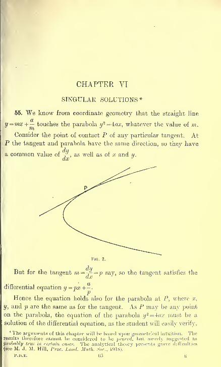
CHAPTER VI
SINGULAR SOLUTIONS*
55. We know from coordinate geometry that the straight line
y =mx + — touches the parabola y2 = iax, whatever the value of m.
Consider the point of contact P of any particular tangent. AtP the tangent and parabola have the same direction, so they have
a common value of -,-, as well as of x and y.
Fig. 7.
But for the tangent m=^-=jp say, so the tangent satisfies the
differential equation y=px+~.
Hence the equation holds also for the parabola at P, where x,
y, and p are the same as for the tangent. As P may be any point
on the parabola, the equation of the parabola y2 = iax must be a
solution of the differential equation, as the student will easily verify.
* The arguments of this chapter will be based upon geometrical intuition. Theresults therefore cannot be considered to be proved, but merely suggested asprobably true in certain cases. The analytical theory presents grave difficulties
(see M. J. M. Hill, Proc. Loud. Math. Soc, 1918).
P.U.E. t)5 B

66 DIFFERENTIAL EQUATIONS
In general, if we have any singly infinite system of curves which
all touch a fixed curve, which we will call their envelope* and if this
family represents the complete primitive of a certain differential
equation of the first order, then the envelope represents a solution
of the differential equation. For at every point of the envelope
x, y, and p have the same value for the envelope and the curve of
the family that touches it there.
Such a solution is called a Singular Solution. It does not
contain any arbitrary constant, and is not deducible from the
Complete Primitive by giving a particular value to the arbitrary
constant in it.
Example for solution.
Prove that the straight line y = x is the envelope of the family of
parabolas y = x + \{x-c) 2. Prove that the point of contact is (c, c),
and that p — \ for the parabola and envelope at this point. Obtain
the differential equation of the family of parabolas in the form
y — x + (p- 1)2
, and verify that the equation of the envelope satisfies this.
Trace the envelope and a few parabolas of the family, taking c as
0, 1, 2, etc.
56. We shall now consider how to obtain singular solutions. It
has been shown that the envelope of the curves represented by the
complete primitive gives a singular solution, so we shall commence
by examining the method of finding envelopes.
The general method t is to eliminate the parameter c between
f(x, y, c) =0, the equation of the family of curves, and
I-E.g. if f(x,y,c) = is y-cx--=0, (1)
|=0 is - * + l=0 (2)
giving c = ± l/^x.
*In Lamb's Infinitesimal Calculus, 2nd ed., Art. 155, the envelope of afamily is defined as the locus of ultimate intersection of consecutive curves of
the family. As thus defined it may include node- or cusp loci in addition to or
instead of what wo have called envelopes. (We shall give a geometrical reason for
this in Art. 56 ; see Lamb for an analytical proof.)
t See Lamb's Infinitesimal Calculus, 2nd ed., Art. 155. If f(x, y, c) is of
the form Lci + Mc + N, the result comes to J\12= 4LN. Tims, for
1 oy - ex - - = 0,9c
'
i. e. c2x - cy + 1 = 0,
the result is y2 = 4x.

SINGULAR SOLUTIONS 67
Substituting in (1), y=±2^/x,or y
2 = 4:X.
This method is equivalent to finding the locus of intersection of
f(x, y, c)=0,
and f(x,y,c + h)=0,
two curves of the family with parameters that differ by a small
quantity h, and proceeding to the limit when h approaches zero.
The result is called the c-discriminant oif(x, y, c) =0.
57. Now consider the diagrams 8, 9, 10, 11.
Fig. 8 shows the case where the curves of the family have
no special singularity. The locus of the ultimate intersections
Fig 8.
PQRSTUV is a curve which has two points in common with each
of the curves of the family (e.g. Q and R lie on the locus and also
on the curve marked 2). In the limit the locus PQRSTUV there-
fore touches each curve of the family, and is what we have defined
as the envelope.
In Fig. 9 each curve of the family has a node. Two con-
secutive curves intersect in three points (e.g. curves 2 and 3 in the
points P, Q, and R).
The locus of such points consists of three distinct parts EE',
AA', and BB'
.
When we proceed to the limit, taking the consecutive curves
ever closer and closer, AA' and BB' will move up to coincidence
with the node-locus iVAT', while EE' will become an envelope. So

68 DIFFERENTIAL EQUATIONS
in this case we expect the c-discriminant to contain the square of
the equation of the node-locus, as well as the equation of the envelope.
E!-^£-»vv«i
Fig. 9.
As Fig. 10 shows, the direction of the node-locus NN' at any
point P on it is in general not the same as that of either branch of
the curve with the node at P. The node-locus has x and y in common
with the curve at P, but not p, so the node-locus is not a solution of
the differential equation of the curves of the family.
Fig. 10.
If the node shrinks into a cusp, the loci EE' and NN' of Fig. 10
move up to coincidence, forming the cusp-locus CC of Fig. 11.
Now NN' was shown to be the coincidence of the two loci AA' and
BB' of Fig. 9, so CC is really the coincidence of three loci, and
its equation must be expected to occur cubed in the c-discriminant.
Fig. 11 shows that the cusp-locus, like the node-locus, is not
(in general) a solution of the differential equation.
K
FIG. 11.
To sum up, we may expect the c-discriminant to contain
(i) the envelope,
(ii) the node-locus squared,
(iii).« the cusp-locus cubed.

SINGULAR SOLUTIONS 69
The envelope is a singular solution, but the node- and cusp-
loci are not (in general *) solutions at all.
58. The following examples will illustrate the preceding results :
Ex. (i). y=p 2.
The complete primitive is easily found to be iy = (x-c) 2,
i.e. c2 -2cx + x2 -±y = 0.
As this is a quadratic in c, we can write down the discriminant at
once as (2z) 2 = 4(a; 2 -4*/),
i.e. y = 0, representing the envelope of the family of equal parabolas
given by the complete primitive, and occurring to the first degree only,
as an envelope should.
y
Flu. 12.
Ex. (ii). %y = 2px-2 V
Proceeding as in the last chapter, we get
i.e. px 2 - 2p 2 = (2x* - ipx)dp
dx'
i.e. a;2 -2p = or p = 2x
dp
dx'.(A)
dx dp— =2 >
x p
* We say in general, because it is conceivable that in some special example a
node- or cusp-locus may coincide with an envelope or with a curve of the family.

70 DIFFERENTIAL EQUATIONS
log x = 2 log p - log c,
cx=p2,
1 8
whence 3y = 2c%* - 2c,
i.e. (3?/ + 2c) 2 = 402?, a family of semi-cubical parabolas with their cusps
on the axis of y.
The c-discriminant is (3y - x3)2 = 9y 2
,
i.e. x3(6?/-x3)=0.
The cusp-locus appears cubed, and the other factor represents the
envelope.
It is easily verified that 6y = x3 is a solution of the differential
equation, while x=0 (giving p = oo) is not.
If we take the first alternative of the equations (a),
i.e. x< 2p=0,
we get by substitution for p in the differential equation
3*/ =4*3,
i.e. the envelope.
This illustrates another method of finding singular solutions.
Examples for solution.
Find the complete primitives and singular solutions (if any) of the
following differential equations. Trace the graphs for Examples 1-4:
(1) ±p 2 -9x = 0. (2) ip 2 (x-2) = l.
(3) xp 2 -2yp + 4x = 0.
(5) p2 + 2xp-y = 0.
(7) ixp 2 + iyp - 1 =0.
(4) ?)2 + ?/
2 -l=0.
(6) xp 2 -2yp + l=0.

SINGULAR SOLUTIONS 71
59. The p-discriminant. We shall now consider how to obtain
the singular solutions of a differential equation directly from the
equation itself, without having to find the complete primitive.
Consider the equation x2p
2 - yp + 1 =0.
If we give x and y any definite numerical values, we get a quad-
ratic for p. For example, if
a = v% y=3, 2^2 -3^ + l=0,
p=\ or 1.
Thus there are two curves of the family satisfying this equation
through every point. These two curves will have the same tangent
at all points where the equation has equal roots in p, i.e. where
the discriminant y2 - 4x2 =0.
Similar conclusions hold for the quadratic Lp2 +Mp+N=0}
where L, M, N are any functions of x and y. There are two curves
through every point in the plane, but these curves have the same
direction at all points on the locus M2 - 4LN =0.
More generally, the differential equation
f(x, y, p) = L p" +LlP"-i +L2p-2 + ... +Ln =0,
where the L's are functions of x and y, gives n values of p for a
given pair of values of x and y, corresponding to n curves through
any point. Two of these n curves have the same tangent at all
points on the locus given by eliminating p from
J{x,y,p)=o,
l -»
for this is the condition given in books on theory of equations for
the existence of a repeated root.
We are thus led to the ^-discriminant, and we must now in-
vestigate the properties of the loci represented by it.
60. The Envelope. The ^-discriminant of the equation
1y=px + ~
or p2x-py + 1=0 f*-
is y2 = ix.
We have already found that the complete primitive consists of
the tangents to the parabola, which is the singular solution. Two
of these tangents pass through every point P in the plane, and
these tangents coincide for points on the envelope.

72 DIFFERENTIAL EQUATIONS
This is an example of the 59-discriminant representing an envelope.
Fig. 15 shows a more general case of this.
FIG. 14.
Consider the curve SQP as moving up to coincidence with the
curve PRT, always remaining in contact with the envelope QRU.The point P will move up towards R, and the tangents to the two
curves through P will finally coincide with each other and with the
tangent at the envelope at R. Thus R is a point for which the p'a
of the two curves of the system through the point coincide, and
consequently the ^-discriminant vanishes.
U
Fig. 15.
Thus the jo-discriminant may be an envelope of the curves of
the system, and if so, as shoAvn in Art. 55, is a singular solution.
61. The tac-locus. The envelope is thus the locus of points
where two consecutive curves of the family have the same value
of p. But it is quite possible for two non-consecutive curves to
touch.
Consider a family of circles, all of equal radius, whose centres
lie on a straight line.

SINGULAR SOLUTIONS 73
Fig. 16 shows that the line of centres is the locus of the point
of contact of pairs of circles. This is called a,, tac-locus. Fig. 17
fig. 16.
shows circles which do not quite touch, but cut in pairs of neigh-
bouring points, lying on two neighbouring loci AA' , BB' . When,
we proceed to the limiting case of contact these two loci coincide
in the tac-locus TT . Thus the ^-discriminant may be expected to
contain the equation of the tac-locus squared.
Fig. 17.
It is obvious that at the point P in Fig. 16 the direction of
the tac-locus is not the direction of the two circles. Thus the
relation between x, y, and p satisfied by the circles will not be
satisfied by the tac-locus, which has the same x and y but a different
p at P. In general, the tac-locus does not furnish a solution of tlie
differential equation.
62. The circles of the last article are represented by
(x + c)2 +y2 =r2
,
if the line of centres is Ox.
This gives x+c = Vr2 -
y
2,
or 1= -yp/Vr2 -y2,
i.e. y2p
2 + y2 r2 =0.
The ^-discriminant of this is y2(y
2 -r2)= 0.
The line y=0 (occurring squared, as we expected) is the tac-
locus, y=±r are the envelopes EE' and FF' of Fig. 16; y = ±r,
giving p=0, are singular solutions of the differential equation, but
y = does not satisfy it.
63. The cusp-locus. The contact that gives rise to the equal
roots in p may be between two branches of the same curve instead

74 DIFFERENTIAL EQUATIONS
of between two different curves, i.e. the ^-discriminant vanishes at
a cusp.
As shown in Fig. 18, the direction of the cusp-locus at any
point P on it is in general not the same as that of the tangent to
the cusp, so the cusp-locus is not a solution of the differential equation.
C'
Fig. 18.
It is natural to enquire if the equation of the cusp-locus will
appear cubed in the p-discriminant, as in the c-discriminant. To
decide this, consider the locus of points for which the two p's are
nearly but not quite equal, when the curves have very flat nodes.
This will be the locus NN' of Fig. 19. In the limit, when the nodes
Fig. 19.
contract into cusps, we get the cusp-locus, and as in this case there
is no question of two or more loci coinciding, we expect the p-
discriminant to contain the equation of the cusp-locus to the first
power only.
64. Summary of results. The ^-discriminant therefore may be
expected to contain
(i) the envelope,
(ii) the tac-locus squared,
4 (iii) the cusp-locus,
and the c-discriminant to contain
(i) the envelope,
(ii) the node-locus squared,
(iii) the cusp-locus cubed.

SINGULAR SOLUTIONS 75
Of these only the envelope is a solution of the differential
equation.
65. Examples.
Ex.(i). ?2(2-3<V)2 = 4(l-t/).
Writing this in the form
fa_ 2-3ydy-
±2V(i-y)'
we easily find the complete primitive in the form
(a>-c)8=ya(l-y).
The c-discriminant and ^-discriminant are respectively
y2(l-y)=0 and (2-3y) 2 (l -y)=0.
1 - y=0, which occurs in both to the first degree, gives an envelope;
y=0, which occurs squared in the c-discriminant and not at all in
the p-discriminant, gives a node-locus ; 2 - Sy = 0, which occurs squared
in the ^-discriminant and not at all in the c-discriminant, gives a
tac-locus.
It is easily verified that of these three loci only the equation of the
envelope satisfies the differential equation.
no. 20.
Ex. (ii). Consider the family of circles
x 2 + y2 + 2cx + 2c 2 -l=0.
By eliminating c (by the methods of Chap. I.), we obtain the differ-
ential equation
2y 2p
2 + 2xyp + x 2 + y2 - 1 =0.

76 DIFFERENTIAL EQUATIONS
The c- and ^-discriminants are respectively
x2 -2(x2 + y2 -l)=0 and x2
y2 -2y2{x2 + y
2 -l)=0,
i.e. x2 + 2y2 -2=0 and y2(x2 + 2y 2 -2)=0.
x2 + 2y2 -2=0 gives an envelope as it occurs to the first degree in
both discriminants, while y = gives a tac-locus, as it occurs squared
in the p-discriminant and not at all in the c-discriminant.
FIG. 2t.
Examples for solution.
In the following examples find the complete primitive if the differ-
ential equation is given or the differential equation if the complete
primitive is given. Find the singular solutions (if any). Trace the
graphs.
(1) ix(x-l){x-2)p 2 -{3x2 -6x + 2)2 = 0. (2) 4*;>
2 -(3z-l) 2 =0.
(3) yp2 -2xp + y = 0. (4) 3xp 2 -6yp + x + 2y=0.
(5) p2 + 2px3 -ix 2y = 0. '6) p
3 -±xyp + 8y 2 =0.
(7) x2 + ?/2 -2c£ + c 2 cos 2 a = 0. (8) c2 + 2cy -x2 + \ = 0.
(9) c2 + (x + y)c + l-xy = 0. (10) x 2 + y2 + 2cxy + c 2 - 1 =0.
66. Clairaut's Form.* We commenced this chapter by con-
sidering the equationy = px +
V
Alexis Claude Clairaut, (if Paris (1713-176,")), although best known in con-
nection with differential equations, wrote chiefly on astronomy.

SINGULAR SOLUTIONS 77
This is a particular case of Clairaut's Form
y=px+f(p) (1)
To solve, differentiate with respect to y,-*.
p=p + {x+f'(p)}-£;
thereforedp
= 0, (2)dx~v
> P = C
or 0=x+f'(p) (3)
Using (1) and (2) we get the complete primitive, the family of
straight lines,y = cx+f(c) (4)
If we eliminate p from (1) and (3) we shall simply get the jo-dis-
criminant.
To find the c-discriminant we eliminate e from (4) and the result
of differentiating (4) partially with respect to c, i.e.
0=x+f(c) (5)
Equations (4) and (5) differ from (1) and (3) only in having c
instead of p. The eliminants are therefore the same. Thus both
disoriminants must represent the envelope.
Of course it is obvious that a family of straight lines cannot
have node-, cusp-, or tac-loci.
Equation (4) gives the important result that the complete primi-
tive of a differential equation of Clairaut's Form may be written down
immediately by simply writing c in place of p.
67. Example.
Find the curve such that OT varies as tan \fs, where T is the point
in which the tangent at any point cuts the axis of x, \Js is its inclination
to this axis, and is the origin.
y
O TI'm. 22.

therefore x-- = kp, •<
78 DIFFERENTIAL EQUATIONS
From the figure, OT =ON-TN=x-y cot \fr
V
V
since tani//-=p;
y
V
i.e. y=px-kp 2.
This is of Clairaut's Form, so the complete primitive is
y = cx- kc 2,
and the singular solution is the discriminant of this,
i.e. x2 = iky.
The curve required is the parabola represented by this singular
solution. The complete primitive represents the family of straight
lines tangent to this parabola.
Examples for solution.
Find the complete primitive and singular solutions of the following
differential equations. Trace the graphs for Examples (1), (2), (4), (7),
(8) and (9).
7(1) y=px+p 2.
y(2) y=px + p3
.
-/
(3) y=px + cosp. (4) y = px + ^{a 2p
2 + b2).
^(5) p=log(px-y). (6) sinpxeos y = coapxsiny+p.
(7) Find the differential equation of the curve such that the tangent
makes with the co-ordinate axes a triangle of constant area k 2, and
hence find the equation of the curve in integral form.
(8) Find the curve such that the tangent cuts off intercepts from
the axes whose sum is constant.
(9) Find the curve such that the part of the tangent intercepted
between the axes is of constant length.
MISCELLANEOUS EXAMPLES ON CHAPTER VI.
Illustrate the solutions by a graph whenever possible.
(1) Examine for singular solutions p2 + 2xp = 3x 2
.
(2) Reduce xyp 2 -(x 2 + y2 -l)p + xy =
to Clairaut's form by the substitution X — x 2; Y = y
2.
Hence show that the equation represents a family of conies touching
the four sides of a square.

MISCELLANEOUS EXAMPLES 79
(3) Show that xyp2 + (x2 -y 2 -h2)p-xy =
represents a family of confocal conies, with the foci at (± h, 0), touching
the four imaginary lines joining the foci to the circular points at infinity.
(4) Show by geometrical reasoning or otherwise that the sub-
stitution x =aX+bY, y = a'X+b'Y,
converts any differential equation of Clairaut's form to another equation
of Clairaut's form.
(5) Show that the complete primitive of 8p3x = y(12p2 -9) is
(x + c)3 = 3y 2
c, the p-discriminant y2 (9x2 -iy2)=0, and the c-dis-
criminant y*(9x2 - 4ty2) = 0. Interpret these discriminants.
(6) Reduce the differential equation
x 2p
2 + yp(2x + y)+y 2 =0, where p = -r-
to Clairaut's form by the substitution £=y, rj = xy.
Hence, or otherwise, solve the equation.
Prove that y + ix = is a singular solution ; and that y=0 is both
part of the envelope and part of an ordinary solution. [London.]
(7) Solve y^iy-Xjj^^ij) » which can be transformed to
Clairaut's form by suitable substitutions. [London.]
(8) Integrate the differential equations :
(i) 3{p + x) 2 = {p-xf.
(ii) y2{\ +ip 2)- 2pxy -1=0.
In (ii) find the singular solution and explain the significance of any
factors that occur. [London.]
(9) Show that the curves of the family
y2 -2cx2y + c 2 (xi -x3)=0
all have a cusp at the origin, touching the axis of x.
By eliminating c obtain the differential equation of the family in
the formip 2x2 (x - 1 ) - ipxy (ix - 3y) + ( 1 6a; - 9) y
2 = 0.
Show that both discriminants take the form x3y2 =0, but that x=0
is not a solution, while y =0 is a particular integral as well as an envelope.
[This example shows that our theory does not apply without modi-
fication to families of curves with a cusp at a fixed point.]
(10) Show that the complete primitive of
represents the family of equal lemniscates of Bernoulli
r 2 = a 2 cos 2(0- a),
inscribed in the circle r = a, which is the singular solution, with the
point r = as a node-locus.

80 DIFFERENTIAL EQUATIONS
(11) Obtain and interpret the complete primitive and singular
solution of/dr\ 2
&)
"
\d6J
(12) Show that r = cd-c2 is the complete primitive and 4r = #2 the
singular solution ofdr /gr \2
r' eTe-\Te)-
Verify that the singular solution touches the complete primitive at
the point (c2
, 2c), the common tangent there making an angle tan-1c
vith the radius vector.

CHAPTER VII
MISCELLANEOUS METHODS FOR EQUATIONS OF THESECOND AND HIGHER ORDERS
68. In this chapter we shall be concerned chiefly with the
reduction of equations of the second order to those of the first
order. We shall show that the order can always be so reduced if
the equation
(i) does not contain y explicitly;
or (ii) does not contain x explicitly;
or (iii) is homogeneous.
A special form of equation, of some importance in Dynamics,
may be reduced by using an integrating factor.
The remainder of the chapter will be devoted to the linear
equation, excluding the simple case, already fully discussed in
Chapter III., where the coefficients are merely constants. It will
be found that the linear equation of the second order can be reduced
to one of the first order if
(i) the operator can be factorised,
or (ii) any one integral belonging to the complementary function
is known.
If the complete complementary function is known, the equation
may be solved by the method of Variation of Parameters. This
elegant method (due to Lagrange) is applicable to linear equations
of any order.
Further information on linear equations, such as the condition
for exact equations, the normal form, the invariantive condition of
equivalence, and the Schwarzian derivative, will be found in the
form of problems among the miscellaneous examples at the end
of the chapter, with hints sufficient to enable the student to work
them out for himself.
P.D.E. 81 K

82 DIFFERENTIAL EQUATIONS
We shall use suffixes to denote differentiations with respect to
dhix, e.g. y2 for tt|, but when the independent variable is any other
than x the differential coefficients will be written in full.
69. y absent. If y does not occur explicitly in an equation of
the second order, write p for yx and J- for y 2 .
We obtain an equation containing onlyJ-, p, and x, and so of
the first order. *
Consider, for example, xy2 +y1= ix.
This transforms into Xj-+p=4:X,
which can be integrated at once
xp = 2x2 + a,
i.e. p = 2x + -.x
By integrating, y = x2 + a log x + b,
where a and 6 are arbitrary constants.
This method may be used to reduce an equation of the nth order
not containing y explicitly to one of the (n - l)th
.
70. x absent. If x is the absent letter, we may still write p for
. , , dp . dp dy dp dp ^yv but for y2 we now write V -fy
, since V dy=TxWy
=^ -y«- The
procedure reduces an equation of the second order without x to one
of the first order in the variables p and y.
For example, W^Vx
transforms into «/])-r=p2
,
from which the student will easily obtain
p=by and y = aehx .
Examples for solution.
(1) 2/ 2 cos2 x = l. (2) yyz+y^-yv I (3) yy 2 + l=yi*.
(4) Reduce to the previous example, and hence solve
(5) xy 3 + y 2= 12x. (6) 2/n - 23/»-i =
gX-
(7) Integrate and interpret geometrically
(i+yi2)* _7g

EQUATIONS OF SECOND AND HIGHER ORDERS 83
(8) The radius of curvature of a certain curve is equal to the lengthof the normal between the curve and the axis of x. Prove that thecurve is a catenary or a circle, according as it is convex or concave tothe axis of x.
(9) Find and solve the differential equation of the curve the lengthof whose arc, measured from a fixed point A to a variable point P, isproportional to the tangent of the angle between the tangent at P andthe axis of x.
*71. Homogeneous equations. If x and y are regarded as of
dimension 1,
yxis of dimension 0,
y2 is of dimension - 1,
y z is of dimension - 2,and so on.
We define a homogeneous equation as one in which all the termsare of the same dimensions. We have already in Chap. II. dealtwith homogeneous equations of the first order and degree, and inChap. III. with the homogeneous linear equation
xnyn +Axn-iyn_x + Bxn~2yn_2 + ...+ Exyx +Ky=0
(where A, B, ... B, K are merely constants), for which we used thesubstitution x = (? or t =log x.
Let us make the same substitution in the homogeneous equation
xijy2 +xy12 =3yy1 (1)
Now v Ji%LjL*yUl dx dt xdt'
^ dx x2 dt x dx dt
_ 1 dy 1 dt d2y
x2 dt x dx dt2
l^dy \_d?y
x2 dt x2 dt2'
Substituting in (1) and multiplying by x, we get
y\dt2 dt)
+\dt)
~ 6ydt'
d2y fdii\ 2
. du
This is an equation, with t absent, similar to those in the last
article with x absent.
Arts. 71-73 may be omitted on a first reading.

84 DIFFERENTIAL EQUATIONS
By putting -tt = ?> the student will easily obtain
yq=2(y2 +b),
giving t+c = l\og(y2 +b).
Hence y2 +b=e^t+c^
= ax4 , replacing e4c by another arbitrary constant a.
72. The example of Art. 71 came out easily because it had no
superfluous a;'s left after associating x2 with y2 and x with yx. In
fact, it could have been written
y(*ty«) +(«&)" -3y(a^i).
But (^+^2)(2/-^i)+a;V«/2
=0 (2)
cannot be so written. To reduce this to a form similar to that of
the last example, put y=vx, a substitution used for homogeneous
equations in Chap. II.
(2) becomes
(x2 + x2v2)(vx - vxx
2 - vx) + xiv2 (xv2 + 2uj) =0,
i.e. -(1 + v2)v1 +v2 (xv2 +2v1)=0, a.
which may be written v2x2v2 = (l -v2)xv1 (3)
"We now proceed as before and put x = e\ giving
dv
dH dv
dfi'dt'
(3) becomes ^--^=(1-^-,AH dv ,.v
l -e'
VcU2 =di>
(4)
an equation with t absent.
, , dv d2v dqAs before, put j-j, &-q&
(4) becomes v2q^=q,
i.e. tq = I (unless q = 0, giving y = ex),
dv vi
and x2v2=—
dv = = 1_1dt
V a v
,, av dv / a2 \,dt = = (o+- av,
v - a \ v-a/
t=av + a2 log (v-a) + b,
and finally log x = ay/x + a2 log (y - ax) - a2 log x + b.

EQUATIONS OF SECOND AND HIGHER ORDERS 85
73. By proceeding as in the last article, we can reduce anyhomogeneous equation of the second order.
Any such equation can be brought to the form
ftyfayi>m/*)-o-
For example, the equation of Art. 71 when divided by x becomes
while that of Art. 72 divided by x3 becomes
(i*5)G-*)+©»-*The substitutions y =vx and x =e* transform
/ (y/x> Vx> xVi) = to / (v, xvx + v, x2v2 + 2xvj) = 0,
j ,r /./ dv d2v dv\ nand then to /^, _ +v,_. +_j =0
,
an equation with t absent, and therefore reducible to the first order.
Examples for solution.
(1) x2y2 -xy1 + y = 0. (2) x2
y2 -xy1 + 5y = 0.
(3) 2x 2yy2 + y
2 = x 2y 1
2.
(i) Make homogeneous by the substitution y = z 2, and hence solve
2x 2yy2 + iy 2 = x 2
y x2 + 2xyyv
74. An equation occurring in Dynamics. The form y2 =f{y)occurs frequently in Dynamics, especially in problems on motion
under a force directed to a fixed point and of magnitude depending
solely on the distance from that fixed point.
Multiply each side of the equation by 2yv "We get
2y1y2= 2f(y)yv
Integrating, y2 = 2
J/ (y) £dx=2]f (y) dy.
This is really the equation of energy.
d2x
dt2
o or
Applying the method to -,
z- = - p
2x, (the equation of simple
harmonic motion), we get
zdtdt2
~ = ~ Zpxdt
Integrating with respect to t,
'dx ,
2(dx 2
( j- ) = -f2x2 + const. =p2 (a2 -x2), say
86 DIFFERENTIAL EQUATIONS
Hence<ti = l 1_dx p \/(a2 -x2 )'
1 . , xt = - sin-1 - + const.,
p a
x = a sin (pt+e).
Examples for solution.
(1) y2= y
3 -y, given that y x=0 when y = \.
(2) y2= e2y
,given that y = and yx
= \ when x=0.
(3) y2= sec 2 y tan y, given that ?/=0 and yx
= \ when x = 0.
"
(l or nd (Lt
(4) tt— -^Tj given that x = A and -r=0 when <= 0.<w 2 x 2 at
[h - x is the distance fallen from rest under gravity varying inversely
as the square of the distance x from the centre of the earth, neglecting
air resistance, etc.]
... d 2u P . .
(5)ffli
+ u =fiw>
m the two cases
(i)P = Hu 2;
(\\)P = ijm*;
given that =-771= when u— ~, where /x, h, and c are constants.
(lu c
[These give the path described by a particle attracted to a fixed
point with a force varying inversely as the square and cube respectively
of the distance r. u is the reciprocal of r, 6 has its ordinary meaning
in polar co-ordinates, /u. is the acceleration at unit distance, and h is
twice the areal velocity. ]
)\ 75. Factorisation of the operator. The linear equation.
(x + 2)y2- (2x+5)y1 + 2y = (x + l)ex
may be written as
{(x + 2)D2 - (2x +5)2) + 2}y = (x + l)ex,
where D stands for -p, as in Chapter III.
Now the operator in this particular example can be factorised,
giving {(x+2)D-l}(D-2)y = (x + l)ex .
Put (D-2)y=v.
Then {(x+2)D -l}0-(x + l)&.
This is a linear equation of the first order. Solving as in Art. 20,
we get v = c{x+2)+ex,
i.e. (D-2)y = c(x+2)+ex,
another linear equation, giving finally
y = a(2x + 5) + be2x - ex , replacing - \c by a.
EQUATIONS OF SECOND AND HIGHER ORDERS 87
Of course it is only in special cases that the operator can be
factorised. It is important to notice that these factors must be
written in the right order, as they are not commutative. Thus, on
reversing the order in this example, we get
(D-2){(x + 2)D-l}y = {(x+2)D2 -(2x + 4)D + 2}y.
Examples for solution.
(1) (x + l)y2 + (x-l) yi -2y=0. (2) xy 2 + (x-\) yi -y = 0.
(3) xy2 + (x-l)y1 -y = x2.
(4) xy2 + (x2 + l)yl + 2xy = 2x, given that y = 2 and yx = whenx=0.
(5) (x2 - 1) y2- (4a; 2 - 3x - 5) y x + (4z 2 - 6x - 5) y = e2x
,given that y = 1
and «/! = 2 when £ = 0.
76. One integral belonging to the complementary function * known.
When one integral of the equation
y2 + Py, + Qy=0 (1)
is known, say y = z, then the more general equation of the second
ordery2 + Py1 + Qy=R, (2)
where P, Q, R are functions of x, can be reduced to one of the first
order by the substitution « _ VZt
Differentiating, y1= v±z + vz1}
y2= v2z+2v1z1 +vz2 .
Hence (2) becomes
t>gz + vx (2z1 +Pz)+v(z2 +Pz1+Qz)=0,
i.e. z^+v^z.+Pz)^, (3)
since by hypothesis z2 + Pz1 +Qz=0.
(3) is a linear equation of the first order in vvSimilarly a linear equation of the nth order can be reduced to
one of the (n - 1)
thif one integral belonging to the complementary
function is known.
77. Example.
Consider again the equation
(x + 2)y 2 -(2x + 5)y 1+ 2y = (x + l)ex (4)
*The proof of Art. 29 that the general solution of a linear differential equation is
the sum of a Particular Integral and the Complementary Function holds good whenthe coefficients are functions of x as well as in the case when they arc constants.

88 DIFFERENTIAL EQUATIONS
If we notice that y = e2x makes the left-hand side of the equation
zero, we can put y = ve2x
giving y 1= (v 1 + 2v)e2x
,
and y2= (v 2 + 4v, + 4v) e2x.
Substitution in (4) gives
(x + 2)v 2e2x + {Mx + 2)-(2x + 5)}v
1e2x
+{i(x + 2)-2(2x + 5)+2}ve2x = (x + l)ex,
dvi.e. (x + 2)j1 + {2x + 3) v 1
= {x + l)e~x
Solving this in the usual way (by finding the integrating factor)
we obtain Vi = e~x + c(x + 2)e~ 2x
.
Integrating, v= - e~x - \c{2x + 5) e~2x + b,
whence y = ve 2x = - ex - ±c(2x + 5) + be2x .
Examples for solution.
(1) Show that y 2 + Pyx+Qy=0 is satisfied by y = ex if 1+P +Q=0,and by y = x if P + Qx = 0.
(2) x2y 2 + xy
1 -y = 8x3 .
(3) x 2y2 -(x
2 + 2x)y1 + (x + 2)y = xsex .
(4) xy2-2 (x + l)y
1 + (x + 2) y = (x-2)e 2x.
(5) x 2y 2 + xy1 -9y = 0, given that y = x* is a solution.
(6) xy 2 (x cos x-2 sin x) +(x2 + 2)yx sin x-2y (x sin z + cos x) =0,
given that y = x2 is a solution.
78. Variation of Parameters. We shall now explain an elegant
but somewhat artificial method for finding the complete primitive
of a linear equation whose complementary function is known.
Let us illustrate the method by applying it to the example
already solved in two different ways, namely,
(x+2)y2 -(2x+5)y1+ 2y = (x + l)e*, ...(1)
of which the complementary function is y = a(2x +5) +be2x.
Assume that y = (2x+5)A +e2xB, (2)
where A and B are functions of x.
This assumption is similar to, but more symmetrical than, that
of Art. 77, viz. : y^^xDifferentiating (2),
y1=(2x +5)A
t+e2xB
l+2A +2e2xB (3)
Now so far the two functions (or parameters) A and B are only
connected by the single equation (1). We can make them satisfy
the additional equation
(2x+5)A1 +e
2xBl=0 (4)

EQUATIONS OF SECOND AND HIGHER ORDERS 89
(3) will then reduce to
y1 =2A+2e2xB (5)
Differentiating (5),
y2 =±eZxB + 2A 1 +2e
2xBl (6)
Substitute these values of y, yv and y2 from equations (2), (5),
and (6) respectively in (1). The co-factors of A and B come to
zero, leaving
2{x+2) Al +2(x + 2)e2xB1 =(x + l)ex (7)
(4) and (7) are two simultaneous equations which we can solve
for Ax and Bv giving
4l Bi
(x + l)ex__ (x + l)erx
e2x~ -(2x +b)~2e2x (x +2)(1 -2x-5)~ 4(z+2)2'
w . (x + l)ex _ ex j 1 1 1•
Mence ^i-4(* +2)«"~Tls+2 (^T2)2/'
€x
and. by integration, A = --r-. ^ + a, where a is a constant.J & 4 (a; +2)
Similarly,
R = (^x+5){x + l)e-x er*_ f _ _1_ _1 I
x ~, 4(z+2)2 "4 I x+2 (ic+2) 2 /'
and B =~{-\-2\+b.4 \x+2 J
Substituting in (2),
y=v*H -i(£2)+a
}+?{^2- 2
l+be"
= a(2x+5)+be2x -ex.
79. Applying these processes to the general linear equation of
the second order,y2 + Py1 + Qy = R, (1)
of which the complementary function au+bv is supposed known,-
a and b being arbitrary constants and u and v known functions of xr
we assume that y=uA+vB, (2)
giving y1=u
lA+v
1B, (3)
provided that uA1+vB
1=0 (4)
Differentiating (3),
y2= u2A + v2B + u1A 1
+vlB
1 (5)
Substitute for y2 , yland y in (1).
The terms involving A will be A(u2 + Pu 1 + Qu), i.e. zero, as by
hypothesis, Wg + p% + qu = .
Similarly the terms involving B vanish, and (1) reduces to
u xA x+v
1B
l=R (6)

90 DIFFERENTIAL EQUATIONS
Solving (4) and (6),—* =A = ^_V -U VUX -UVX
*
We then get A and B by integration, say
A=f(x)+a,
B=F(x)+b,where / (x) and F (x) are known functions of x, and a and 6 are
arbitrary constants.
Substituting in (2), we get finally
y = uf(x) +vF (x) + au + bv.
* 80. This method can be extended to linear equations of any
order. For that of the third order,
y 3 + Py2 + Qy1 + Ry=S, (1)
of which the complementary function y = au +bv+cw is supposed
known, the student will easily obtain the equations
y = uA+vB+wC, (2)
y1 =u1A +v1B+w1C, (3)
provided that 0=uA 1 +vB1+ivC1 ; (4)
hence y2= u2A+v2B +w2C, (5)
provided that 0=u1A1 +v1B1 +w1C1 ; (6)
then yz- u 3A + v 3B +w 3C
+ u2A 1 +v2B1 +w2C1 ; (7)
by substitution in(l), S=v2A1 +v2B1 +w2C1 (8)
A ly Bly and Cxare then found from the three equations (4), (6)
and (8).
Examples for solution.
(1) 2/2 + V = cosec x. (2) y 2 + iy = 4 tan 2z.
<3) y*-y=rh'(4) x 2
y 2 + xy x- y = x 2
ex
,given the complementary function ax + bx*1
.
(5) y3 -6ij 2 +n yi -6y = e2 *.
81. Comparison of the different methods for solving linear equations.
If it is required to solve a linear equation of the second order and
no special method is indicated, it is generally best to try to guess
a particular integral belonging to the complementary function and
proceed as in Art. 76. This method may be used to reduce a linear
equation of the nth order to one of the (n - l)th
.
* To be omitted on a first reading.
EQUATIONS OF SECOND AND HIGHER ORDERS 91
The method of factorisation of the operator gives a neat solution
in a few cases, but these are usually examples specially constructed
for this purpose. In general the operator cannot be factorised.
The method of variation of parameters is inferior in practical
value to that of Art. 76, as it requires a complete knowledge of the
complementary function instead of only one part of it. Moreover,
if applied to equations of the third or higher order, it requires too
much labour to solve the simultaneous equations for A x> Bv Cx , etc.,
and to perform the integrations.
MISCELLANEOUS EXAMPLES ON CHAPTER VII.
(1) 2/^2 ~2/i2 + 2/i
= 0. <2) xy2 + xy12 -y
1 = 0.
(3) y»*r*y*-v (4) y„ + «/„- 2 = 8cos3z.
(5) (x 2 log x -
x
2)y 2 - xy t + y = 0.
(6) (x2 + 2x -l)y 2- (3x 2 + 8x -l)y 1 + (2x 2 + 6x)y = 0.
(7) Verify that cos nx and sin nx are integrating factors of
y 2 + n 2y=f{x).
Hence obtain two first integrals of
y 2 + n 2y = sec nx,
and by elimination of y xdeduce the complete primitive.
(8) Show that the linear equation
Ay + By 1 + Cy 2 + ...+Syn = T,
where A, B, C, ... T are functions of x, is exact, i.e. derivable imme-diately by differentiation from an equation of the next lower order, if
the successive differential coefficients of A, B, C, ... satisfy the relation
A-B1+ C 2 -...+(-l)
nSn = 0.
[N.B.—By successive integration by parts,
]Syndx = Syn^ 1 -S 1yn_ 2 + S2yn_ 3 + ...+(-l)n-1Sn_ 1y + }(-l)nSn ydx.]
Verify that this condition is satisfied by the following equation, and
hence solve it
:
(2x 2 + 3x) y 2 + (6x + 3)y 1 + 2y = (x + l)ex .
(9) Verify that the following non-linear equations are exact, and
solve them: (i) yy 2 + yi2 = 0.
(ii) xyy 2 + xy12 + tjy
1= 0.
(10) Show that the substitution y = ve •>
IXtransforms
y2 + Py 1 +Qy = R,
where P, Q, and R are functions of x, into the Normal Form
v2 + Iv = S,
92 DIFFERENTIAL EQUATIONS
where I=Q-\PX -\P\
and S = Re^Pdx
.
Put into its Normal Form, and hence solve
y2 -ixy 1 + (4:X2 -l)y= - 3ex*sin 2x.
(11) Show that if the two equations
and z2 + pz 1 + qz =
reduce to the same Normal Form, they may be transformed into
each other by the relation
\[pdx \\pdx
i.e. the condition of equivalence is that the Invariant I should be the
same.
(12) Show that the equations
x2y2 + 2(xz -x)y
1 + (l-2x2)y=0and x 2z 2 + 2(x3 + x)z l -{l-2x 2)z=0
have the same invariant, and find the relation that transforms one into
the other. Verify by actually carrying out this transformation.
(13) If u and su are any two solutions of
v 2 + lv = 0, (1)
prove that ^ = _2^1, (2)s1
u
and hence that ^-^(-2Y = 2/ (3)
From (2) show that if s is any solution of (3), s^ and ss^ are
solutions of (1).
[The function of the differential coefficients of s on the left-hand
side of (3) is called the Schivarzian Derivative (after H. A. Schwarz of
Berlin) and written {s, x}. It is of importance in the theory of the
Hypergeometric Series.]
(14) Calculate the Invariant / of the equation
x 2y 2- (x2 + 2x)y
x+ (x + 2)y=Q.
Taking s as the quotient of the two solutions xex and x, verify that
{s,x} = 21,
and that s xand ssf* are solutions of the Normal Form of the original
equation.
(15) If u and v are two solutions of
y2 +Pyi+Qy=o,prove that uv2
- vu 2 + P{uv 1- vuj) = 0,
and hence that uv1 -vu 1— ae * .
Verify this for the equation of the last example.

MISCELLANEOUS EXAMPLES 93
(16) Show that yy x= const, is a first integral of the equation formed
by omitting the last term of
By putting yyx= C, where C is now a function of x (in fact, varying
the parameter C), show that if y is a solution of the full equation, then
c[=-y 2,
and hence C 2 = const. - \y*,
giving finally y2 = a sin {x\J1 + b).
[This method applies to any equation of the form
*+*/(*) +*(y)-o.]
(17) Solve the following equations by changing the independent
variable :
d2ti Q'V
(ii) (l+*«)»g +2»(l+^+4y-a
(18) Transform the differential equation
j~2 cos x + ~j~ sm x ~ %y cos3 X
=
^ c°s5 £
into one having z as independent variable, where
z = sin x,
and solve the equation. [London.]
(19) Show that if z satisfies
^ +P-=0,dx2 dx
by changing the independent variable from x to z, we shall transform
intod4
+ Sy=T'
Hence solve + (l -^)^ + ix 2ye- 2x = 4:(x 2 + x3)e-Zx .

CHAPTER VIII
NUMERICAL APPROXIMATIONS TO THE SOLUTION OFDIFFERENTIAL EQUATIONS
82. The student will have noticed that the methods given in the
preceding chapters for obtaining solutions in finite form only apply
to certain special types of differential equations. If an equation
does not belong to one of these special types, we have to use approxi-
mate methods. The graphical method of Dr. Brodetsky, given in
Chapter L, gives a good general idea of the nature of the solution r
but it cannot be relied upon for numerical values.
In this chapter we shall first give Picard's * method for getting
successive algebraic approximations. By putting numbers in these,
we generally get excellent numerical results. Unfortunately the
method can only be applied to a limited class of equations, in which
the successive integrations can be easily performed.
The second method, which is entirely numerical and of muchmore general application, is due to Runge.f With proper pre-
cautions it gives good results in most cases, although occasionally
it may involve a very large amount of arithmetical calculation. "We
shall treat several examples by both methods to enable their merits
to be compared.
Variations of Runge's method have been given by Heun, Kutta,
and the present writer.
83. Picard's method of integrating successive approximations. The
differential equation dv
* E. Picard, Professor at the University of Paris, is one of the most distinguishedmathematicians of to-day. He is well known for his researches on the Theory ofFunctions, and his Cours (Tanalyse is a standard text-book.
t C. Runge, Professor at the University of Gottingen, is an authority ongraphical methods.
94

NUMERICAL APPROXIMATIONS 9fr
where y =6 when x-a, can be written
*/ = & +[f(x,y)dx.
For a first approximation we replace the y inf(x, y) by b ; for
a second we replace it by the first approximation, for a third by thesecond, and so on.
duEx. (i). J?- = x + y
2, where y=0 when x=0.
Here y = I (x + y2) dx.
Jo
First approximation. Put ?/=0 in x + y2,giving
y=\ xdx = \x2.
Jo
Second approximation. Put ?/ = \x2 va.x + y2
, giving
ry = (» + iz4
) (far = \x2 + z\x5 .
Jo
Third approximation. Put i/ = \x2 + -^V^5 in cc + «/
2,giving
r1/ = (a? +\& + -itx
1 + Thvx10) dx
Jo— ir2 i 1 r5 i 1 y8 i l yll—
2 X ^W*' + TTRr,c + TTTTD"X >
and so on indefinitely.
where t/ = l and z = £ when cc=0.
Here ?/ = l + l 2^ and z = i+l x3(y + z)dx.
Jo Jo
First approximation.
y=*l + I -^cfa; = l+£x,Jo"
z = \ + [V(l +|) cfc^ + fz4 .
Jo
Second approximation.
y = l + [ (% + %xi)dx = l+±x + Ts1Tx5,
96 DIFFERENTIAL EQUATIONS
Third approximation.
y- 1 + f (£+ fx* + -As5 + frx*) dxJo
- 1 + \x+^z5 + isVz6 + Tfox
9,
z=4 + r a»(4 + \x + f
z
4 +^r5 + -fox8) dx
Jo
and so on.
Ex. (iii). j^ = x3 (^- + y), where */ = l and -j-=\ when x=0.
By putting j-~z, we reduce this to Ex. (ii).
It may be remarked that Picard's method converts the differential
equation into an equation involving integrals, which is called an Integral
Equation.
Examples for solution.
Find the third approximation in the following cases. For examples
(1) and (2) obtain also the exact solution by the usual methods.
\/ (1) ~ = 2y - 2x2 - 3, where y = 2 when x = 0.CLOC
(2) -~ = 2--, where v = 2 when x = l.dx x
ft-"*-.
where y = 2 and z=0 when x = 0.
(dy
(4)
dx~Z'
dz a .-1-=x2z + x*y,dx
9
where y = 5 and 2 = 1 when x=0.
(5)y = xzJ- + tfy where y = 5 and / = 1 when x=0.
v ' dx2 dx * * dx
84. Determination of numerical values from these approximations.
Suppose that in Ex. (i) of the last article we desire the value of y,
correct to seven places of decimals, when x =0-3.
Substituting x =0-3, we get \ (0-3)2 =0-045 from the first approxi-
mation.
The second adds ^(0-3)5 =0-0001215,
while the third adds ^(O^)8 + ttVtf(0-3)u =0-00000041 ... .

NUMERICAL APPROXIMATIONS 97
Noticing the rapid way in which these successive increments
decrease, we conclude that the next one will not affect the first
seven decimal places, so the required value is 0-0451219... .
Of course for larger values of x we should have to take more
than three approximations to get the result to the required degree
of accuracy.
We shall prove in Chap. X. that under certain conditions the
approximations obtained really do tend to a limit, and that this limit
gives the solution. This is called an Existence Theorem.
Example for solution.
(i) Show that in Ex. (ii) of Art. 83, x = 0-5 gives y = 1-252... and2=0-526... , while z=0-2 gives y = 1-100025... and 2 = 0-500632... .
85. Numerical approximation direct from the differential equation.
The method of integrating successive approximations breaks down
if, as is often the case, the integrations are impracticable. But
there are other methods which can always be applied. Consider
the problem geometrically. The differential equation
dy
dx =/fo y)
determines a family of curves (the " characteristics ") which do not
intersect each other and of which one passes through every point
Fig. 23.
in the plane.* Given a point P (a, b), we know that the gradient
of the characteristic through P is f (a, b), and we want to determine
* This is on the assumption that f(x, y) has a perfectly definite value for every
point in the plane. If, however, f(x, y) becomes indeterminate for one or morepoints, these points are called singular points of the equation, and the behaviourof the characteristics near such points calls for special investigation. See Art. 10.

98 DIFFERENTIAL EQUATIONS
the y =NQ of any other point on the same characteristic, given that
x =ON = a + h, say. A first approximation is given by taking the
tangent PR instead of the characteristic PQ, i.e. taking
y =2VX +LR=NL+PL tan /_RPL = b+hf{a, b) =b + hf , say.
But unless h is very small indeed, the error RQ is far from
negligible.
A more reasonable approximation is to take the chord PQ as
parallel to the tangent to the characteristic through S, the middle
point of PR.
Since <# is (a + \h, b + %hf ), this gives
y =NL +LQ=NL + PL tan /_QPL =b+hf{a + \h, b +ffi ).
This simple formula gives good results in some cases, as will be
seen from the following examples :
Ex. (i) -^-= x + y2
;given that y=0 when x = 0, required y when
a; = 0-3.dx
Here a = 6 = 0, A = 0-3, f(x,y)=x + y*.
Therefore
/o=/(a,6)=0, a + £A = 0-15, 6 +P/ = 0,
giving b + hf{a + \h, 6 + ^/ )=0 + 0-3 x/(0-15, 0) =0-045.
The value found in Art. 84 was 0-0451219... , so the error is
0-00012... , about J per cent.
Ex. (ii). -j- = 2 - -;given that y — 2 when x = l, find y when x = 1 -2.
Here o-l, 6 = 2, A=0-2, / =2-f=0.
Therefore b + hf(a + $h, 6 + ^/ ) = 2 + 0-2 x/(M, 2)
= 2+0-2 x (2--^-) =2-036....
Now the differential equation is easily integrable, giving y = x + -,
so when a? = 1-2 the value of y is 2-033... . The error is 0-003... , which
is rather large compared with the increment of y, namely 0-036... .
Ex. (iii). -g = «=/(&, y, z), say,
-^ = x3(y + z)~g(x, y, 2), say;
given that y = \ and 2 = 0-5 when x = 0, find y and 2 when x = 0-5.
Here a=0, 6 = 1, c (the initial value of 2) =0-5, A=0-5.
Hence / =/(0, 1, 0-5) =0-5; g =g<0, 1, 0-5)=0.

NUMERICAL APPROXIMATIONS 99
By an obvious extension of the method for two variables, we take= b + hf{a + \h, b + \hf ,
c +^ ) = l+0-5x/(0-25, 1-125, 0-5) = l-2500,and z = c + hg(a + $h, b + Wo> c + ihgQ)
=0-5 +0-5x0(0-25, 1-125, 0-5) =0-5127.The accurate values, found as in Art. 84, are
y = 1-252... and 2=0-526....Thus we have obtained a fairly good result for y, but a verv bad
one for z.J
kThe
il
unJcer*aiuty ab°ut the degree of accuracy of the result deprives
the method of most of its value. However, it forms an introduction to
articb°
re e meth°d 0f RunSe >t0 be explained in the next
Examples for solution.
.-. dy i
{)dx= {x ~
y)~ 1; ^ven that y = 4 when x = 2-3, obtain the value
y= 4-122 when z = 2-7. [Runge's method gives 4-118.]
in\ dy 1 ${) di^lO™
- 1+lo&(x + y)}'> given that y = 2 when x=-l, obtain
;he value y = 2-194 when a-1. [Runge's method gives 2-192.]
ti\dy y •
{)ti'<
x'glventhat 2/ = 2whenz = l, obtain the valuey = 2-076
X ion2
:..^ show that y =l
x2+i>
so that when - 1* V ™
86. Runge's method. Suppose that the function of y defined * by
~dx~$^' $' y =b when x = a
>
3 denoted by y=F(x).If this can be expanded by Taylor's theorem,
F(a + h) =F{a) + hF{a) +^F"(a) +~F'"(a) + ... .
Now F\x)=%=f{x,y)=f,^y.
We shall now take the total differential coefficient with respect>x (that is, taking the y in/ to vary in consequence of the variation
i x).^Let us denote partial differential coefficients by
p-f?, ,-§?, rJ-f s-^f t-d2f-
to' * dy' dx*'S~dxdy'
t
dtf>id their values when x = a and y =b by Po , qQ , etc.
io^IinodZ.Tt' ThlCh th« diffe^«al equation and the initial con-« «?lu
7i * 1 • f
functl0n are discussed in Chap. X. The graphical treatnt of the last article assumes that these conditions are satisfied
graptU°al treat"

100 DIFFERENTIAL EQUATIONS
Similarly, *»<(*) =(| +| J) (,+,,)
=r+^+/s+/(s+ ?2+/|F).
Thus
JP(a+A)-.F(a)
= fc/ + JA8(p +/o?o) +#"(*• +2/>o +/o% +M> +/o?o
2) + ••• • (1)
The first term represents the first approximation mentioned and
rejected in Art. 85.
The second approximation of Art. 85, i.e.
y-b=hf{a+\h,b + \hfQ ) = k1} say,
may now be expanded and compared with (1).
Now, by Taylor's theorem for two independent variables,
f(a+lh,b+±hf )x
=/o +1% + Wtfo +2! (^
2/"o + hh2Uo + iWo) + • • • >
giving A;1 =A/ +^2(^o+/o?o)+^
3K+2/oSo4o) + (2)
It is obvious that Jcx
is at fault in the coefficient of h3.
Our next step is suggested by the usual methods * for the
numerical integration of the simpler differential equation
!=/(*>
Our second approximation in this case reduces to the Trapezoidal
Rule y-b=hf{a+\h).
Now the next approximation discussed is generally Simpson's
Rule, which may be written
y-&-i*{/(a)+4/(a+#)+/(a + *)}.
If we expand the corresponding formula in two variables, namely
\Hh + tfiP+\K b+lhf^+fia+h, b + hf )},
we easily obtain
¥o + ¥i2(Po+foqo)+hW(ro + 2foSo + t
) + ---, (3)
which is a better approximation than kv but even now has not the
coefficient of h3 quite in agreement with (1).
To obtain the extra terms in h3, Runge f replaces
hf(a+h,b+hf )
* See the text- books on Calculus by Gibson or Lamb,
f Mathematische Annalen, Vol. XLVI. pp. 167-178.

NUMERICAL APPROXIMATIONS 101
by V" = hf(a +h,b+ V), where k" = hf(a + h,b+ hf ). The modified
formula maybe briefly written ^{k' +ikl +k'"}, where k' =hf , or
fkx + ^k2 = kx + 1 (k2- kj), where k2
= \(k' +k'").
vThe student will easily verify that the expansion of Runge's
formula agrees with the right-hand side of (1) as far as the terms
in h, h2, and h3 are concerned.
Of course this method will give bad results if the series (1) con-
verges slowly.
Ifyo> 1 numerically, we rewrite our equation
i=Khr F(x
' y) - m '
and now F < 1 numerically, and we take y as the independent
variable.
87. Method of solving examples by Runge's rule. To avoid
confusion, the calculations should be formed in some definite order,
such as the following :
Calculate successively k' =hf ,
k"=hf{a + h,b+k'),
k"'=hf(a + h,b+k"),
k^hfia + ih, 6+P'),k2 = 2 \k +k ),
and finally k = k1 +^(k2 -k1 ).
Moreover, as kx is itself an approximation to the value required,
it is clear that if the difference between k and kv namely I (k2- kx ),
is small compared with k± and k, the error in k is likely to be even
smaller.
dyEx. (i). j-=x + y
2;
given that y=0 when x = 0, find y when x = 0-3.
Here a = 0, 6 = 0, A = 0-3, f(x,y)=x + y2
, / = 0;
tf-Vo-0;k" = hf{a + h, & + A/)=0-3x/(0-3, 0)=0-3x0-3 =0-0900;
k'" = hf(a + h, b + k") =0-3 x/(0-3, 0-09) =0-3 x (0-3 + 0-0081) =0-0924;
kx -hf{a + \h, 6 + P') =0-3 x/(0-15,0) =0-3x0-15 =0-0450;
k2= \(k' + k'") = \x 0-0924 =0-0462;
and
k = kx +£(& 2 -fc 1 ) =0-0450 + 0-0004 =0-0454.
As the difference between k = 0-0454 and kx= 0-0450 is fairly small
compared with either, it is highly probable that the error in k is less

102 DIFFERENTIAL EQUATIONS
than this difference 0-0004. That is to say, we conclude that the value
(
is 0-045, correct to the third place of decimals.
We can test this conclusion by comparing the result obtained in
Art. 84, viz. 0-0451219... .
fjbti II — nt*
Ex. (ii). j- ; given that y = \ when sc= 0, find y when x= l.(too y *t" x
This is an example given in Eunge's original paper. Divide the
range into three parts, to 0-2, 0-2 to 0-5, 0-5 to 1. We take a small
increment for the first step because / (x, y) is largest at the beginning.
First step. a = 0, 6= 1, /* = 0-2, / = 1;
k' = hf =0-200
k" = hf(a + h, b + k') =0-2 xf (0-2, 1-2) =0-143
k'" = hf{a + h, b + k")=0-2xf(0-2, 1-143) =0-140
k x= hf(a + \h,b + \k')=0-Zxf{0-\, 1-1) =0-167
k 2= ^{k' + k'") = ^x 0-340 =0-170
and k^^ +H^-kj) =0-167 +0-001 =0-168
giving i/ = l-168 when z = 0-2.
Second step.
a = 0-2, 6 = 1-168, 7*=0-3, / =/(0-2, 1-168) =0-708.
Proceeding as before we get i1= 0-170, &2
= 0-173 and so £ = 0-171,
giving y = 1-168 +0-171 = 1-339 when x = 0-5.
Third step. a = 0-5, 6 = 1-339, 7j = 0-5.
We find k t= k 2
= k = 0-160, giving i/ = l-499 when x = l.
Considering the k and kv the error in this result should be less than
0-001 on each of the first and second steps and negligible (to 3 decimal
places) on the third, that is, less than 0-002 altogether.
As a matter of fact, the true value of y is between 1 -498 and 1 -499,
so the error is less than 0-001. This value of y is found by integrating
the equation, leading to
7T - 2 tan-1 ^ = loge (x2 + y
2).
Examples for solution.
Give numerical results to the following examples to as many places
of decimals as are likely to be accurate :
(1) y = 77;{y -1 +l°ge(3 + 2/)} ;given that y = 2 when x= -1, find
y when x = l, taking h = 2 (as /is very small).,
(2) Obtain a closer approximation to the preceding question bytaking two steps.
(3) ~ = (x2 -y) -1;
given that y = i when x = 2 -3, find y when
x = 2 -7 (a) in one step, (6) in two steps.

NUMERICAL APPROXIMATIONS 103
dtf V(4) Show that if -^=2-- and y = 2 when as—1, then y = x + -.
dx X X
Hence find the errors in the result given by Runge's method, taking
(a) ^=0-4, (b) h=0-2, (c) h=0-l (a single step in each case), and compare
these errors with their estimated upper limits.
(5) If E(h) is the error of the result of solving a differential equation
of the first order by Runge's method, prove that
LtEW _ I
h.+o E{nh) n*'
Hence show that the error in a two-step solution should be about§ of that given by one step ; that is to say, we get the answer correct
to an extra place of decimals (roughly) by doubling the number of steps.
88. Extension * to simultaneous equations. The method is easily
extended to simultaneous equations. As the proof is very similar
to the work in Art. 86, though rather lengthy, we shall merely give
an example. This example and those given for solution are taken,
with slight modifications, from Runge's paper.
Ex. £= 22 -|=/(x, y, z), say,
dz y .
given that y= 0-2027 and 2 = 1-0202 when x = 0-2, find y and z whenz = 0-4.
Hereo = 0-2, 6=0-2027, c = 1-0202, /„=/ (0-2, 0-2027, 1-0202) = 1-027,
a = 0-2070, A = 0-2;
k' = hf = 0-2x 1-027 =0-2054
Z' =^ = 0-2x 0-2070 =0-0414
k" = hf(a + h, b + k', c + V) =0-2 x/(0-4, 0-4081, 1-0616) =0-2206
l" = hg(a + h, b + k', c + l') =0-2 xo(0-4, 0-4081, 1-0616) =0-0894
k'" = hf(a + h, b + k", c + O=0-2x/(0-4, 0-4233, 1-1096) =0-2322
l'" = hg(a + h, b + k", c + l") =0-2 xo(0-4, 0-4233, 1-1096) =0-0934
kj_ = hf(a + \h, b + p', c + \V) =0-2 x/(0-3, 0-3054, 1 -0409) =0-2128
l^hfia + lh, b + \lc', c + \l') =0-2xo(0-3, 0-3054, 1-0409) =0-0641
k2= $(k' + k'") =0-2188
12= \{V + V") =0-0674
k = k1 + ^(k 2 -k 1)= 0-2128 + 0-0020 =0-2148
l = ^ + l(l 2 -Ji) =0-0641 +0-0011 =0-0652
giving y = 0-2027 +0-21 48 = 0-41 75
and 2 = 1 -0202 + -0652 = 1 -0854,
probably correct to the third place of decimals.
*The rest of this chapter may be omitted on a first reading.
104 DIFFERENTIAL EQUATIONS
Examples for solution.
(1) With the equation of Art. 88, show that if y =04175 and2 = 1-0854 when x =0-4, then y =0-6614 and 2 = 1-2145 (probably correct
to the third place of decimals) when x = 0-6.
... dw _ V(l-w2) dr w . ,
(2) — =-2« + -^ '-; j-^—^z rx ;
given that w =0-7500dz r dz v(l ~ w )
and r=0-6 when 2 = 1-2145, obtain the values w =0-5163 and r =0-7348when 2 (which is to be taken as the independent variable) = 1-3745.
Show that the value of r is probably correct to four decimal places, butthat the third place in the value of iv may be in error.
(3) By putting w = cos<f>
in the last example and t/ = sin <p, x= r in
the example of Art. 88, obtain in each case the equations
dz _ sin d> d<h^- = tanrf>; 22 = - + cos<b-r-,dr r
r T dr
which give the form of a drop of water resting on a horizontal plane.
89. Methods* of Heun and Kutta. These methods are very
similar to those of Runge, so we shall state them very briefly. The
problem is : given that -~ =f(x, y) and y=b when x = a, to find
the increment h of y when the increment of x is h.
Heun calculates successively
k'=hf(a,b),
k"=hf(a+ih,b+lk'),
Jc'"=hf(a + %h,b+ik"),and then takes l(k' +SJc'") as the approximate value of h.
Kutta calculates successively,
k'=hf(a,b),
Jc"=hf{a+ih,b+ik'),
k'"=hf(a+lh,b+k" -\k'),
k""=hf(a+h,b+k"'-k"+k'),and then takes |(&' +3k" +3k'" +k"") as the approximate value
oik.
The approximations can be verified by expansion in a Taylor's
series, as in Runge's case.
Example for solution.
n/'U <u nr
Given that -f-=- and y — \ when x=0, find the value of y (to 8
significant figures) when x = 1-2 by the methods of Runge, Heun, andKutta, and compare them with the accurate value 1-1678417. [FromKutta 's paper. ]
* Zeitschrift fur Mathematik und Physik, Vols. 45 and 46.

NUMERICAL APPROXIMATIONS 105
90. Another method, with limits for the error. The present writer
has found * four formulae which give four numbers, between the
greatest and least of which the required increment of y must lie.
A new approximate formula can be derived from these. Whenapplied to Runge's example, this new formula gives more accurate
results than any previous method.
The method is an extension of the following well-known results
concerning definite integrals.
91. Limits between which the value of a definite integral lies. Let
F(x) be a function which, together with its first and second
differential coefficients, is continuous (and therefore finite) between
x=a and x=a + h. Let F"{x) be of constant sign in the interval.
In the figure this sign is taken as positive, making the curve concave
upwards. LP, MQ, NR are parallel to the axis of y, M is the
middle point of LN, and SQT is the tangent at Q. OL=a, LN = h.
3
Rs~-^^Q
T
MFIG. 24.
Then the area PLNR lies between that of the trapezium SLNTand the sum of the areas of the trapezia PLMQ, QMNR.
ThatCa+k
is, F(x)diJ a
ix lies between
hF{a + \h)=A, say,
and lh{F(a)+2F(a + lh)+F(a+h)}=B, say.
In the figure F"(x) is positive and A is the lower limit, B the
upper. If F"(x) were negative, A would be the upper limit and Bthe lower.
* Phil. Mag., June 1919. Most of this paper is reproduced here.

106 DIFFERENTIAL EQUATIONS
As an approximation to the value of the integral it is best to
take, not the arithmetic mean of A and B, but %B+^A, which is
exact when PQR is an arc of a parabola with its axis parallel to the
axis of x. It is also exact for the more general case when
F (x) = a + bx + ex2 + ex3,
as is proved in most treatises on the Calculus in their discussion of
Simpson's Rule.
92. Extension of preceding results to functions denned by differential
equations. Consider the function denned by
^ =»/(*» y)> y= b wnen *
=
a ;
where f(x, y) is subject to the following limitations in the range of
values a to a + h for x and 6 - h to b + h for y. It will be seen from
what follows below that the increment of y is numerically less than h,
so that all values of y will fall in the above range. The limitations
are :
(1) f(x, y) is finite and continuous, as are also its first and second
partial differential coefficients.
(2) It never numerically exceeds unity. If this condition is not
satisfied, we can generally get a new equation in which it is satisfied
by taking y instead of x as the independent variable.
(3) Neither cPy/dx3 nor df/dy changes sign.
" Let m and M be any two numbers, such that
Then if the values of y when x is a +\h and a + h are denoted by
b +j and b + h respectively,*
-^h^lmh<j<^Mh^ih, (1)
and -&= mh<k<Mh^h (2)
We shall now apply the formulae of the last article, taking y to
be the same function as that defined byCa+x
y = b +\
F(x)dx,J a
Ca+h
so that &=| F(x)dx.
We have to express the formulae in terms of / instead of F.
Now, F(a) =the value of dy/dx when x = a,
so that F(a)=f(a, b).
*The following inequalities hold only if h is positive. If h is negative, they
must be modified, but the final result stated at the end of this article is still true.

NUMERICAL APPROXIMATIONS 107
Similarly, F(a + \h) =f(a + \h, b +j),
and F(a + h)=f(a+h, b + k).
Now, if df/dy is positive, so that/ increases with y, the inequalities
<1) and (2) lead to
f{a+\h, b+\mh)<f(a + \h, b+j)<f(a+\h, b+\Mh), (3)
and f(a+h,b+mh)<f(a + h,b+k)<f(a + h,b+Mh); (4)
while if df/dy is negative,
/(a + \h, b + \mh) >f(a + %h, b +j)>f(a + \h, b + \Mh), ... (5)
and f(a+h,b+mh)>f(a+h,b+k)>f(a + h,b+Mh) (6)
Thus if F" (x) — dPy/dx3 is positive and df/dy is also positive, the
result of Art. 91,
A<k<B,may be replaced by p<k<Q, (7)
where p = hf(a + \h, b + \mh)
and Q = \h{f{a, b) + 2f(a + ±h,b+ \Mh) +f{a + h,b+Mh)};
while if F" (x) is positive, and df/dy is negative,
P<k<q, (8)
where P = hf(a + \h, b + \Mh)
and q = \h{f{a, b) + 2f(a + hh, b + ^mh) +f(a + h, b+ mh)}.
Similarly, if F" (x) and df/dy are both negative,
p>k>Q, (9)
while if F" {x) is negative and df/dy positive,
P>k>q (10)
These results may be summed up by saying that in every case
{subject to the limitations on/ stated at the beginning of this article)
k lies between the greatest and least of the four numbers p, P, q, and Q.
As an approximate formula we use k= %B+^A, replacing B by
Q or q, and A by p or P.
93. Application to a numerical example. Consider the example
selected by Runge and Kutta to illustrate their methods,
-t~=- ; w = lwhena;=0.ax y + x a
It is required to find the increment k of y when x increases by
0-2. Here f(x, y)=(y -x)/(y +x). This function satisfies the con-
ditions laid down in the last article.*
WetakeM = l, m = (l-0-2)/(l-2+0-2)=4/7.
* As f (x, y) is positive, y lies between 1 and 1-2. When finding M and m wealways take the smallest range for y that we can find

108 DIFFERENTIAL EQUATIONS
Then p =0-1654321,
P =0-1666667,
9=0-1674987,
£=0-1690476.
Thus h lies between p and Q. Errors.
|Q + *p =0-1678424, 00000007
Kutta's value 0-1678449, 0-0000032
Kunge's value 0-1678487, 0-0000070
Heun's value 0-1680250, 0-0001833
The second, third, and fourth of these were calculated by Kutta.
Now this particular example admits of integration in finite terms,
giving
log {x2 +y2)-2 tan-1 (x/y) =0.
Hence we may find the accurate value of k.
Accurate value =0-1678417.
Thus in this example our result is the nearest to the accurate
value, the errors being as stated above.
We may also test the method by taking a larger interval h = \.
Of course a more accurate way of obtaining the result would be to
take several steps, say ^=0-2, 0-3, and finally 0-5, as Runge does.
Still, it is interesting to see how far wrong the results come for
the larger interval.
We take M = 1, m = (l -l)/(2 +1) =0.
Then iQ+iP =0-50000.
True value =0-49828, Errors.
Kutta's value =0-49914, 0-00086
Our value =0-50000, 0-00172
Heun's value =0-51613, 0-01785
Runge's value =0-52381, 0-02553
This time Kutta's value is the nearest, and ours is second.

CHAPTER IX
SOLUTION IN SERIES. METHOD OF FROBENIUS
94. In Chapter VII. we obtained the solution of several equations
of the form d2y n dy n A
where P and Q were functions of x.
In every case the solution was of the form
y=af(x)+bF(x),
where a and b were arbitrary constants.
The functions f(x) and F(x) were generally made up of integral
or fractional powers of x, sines and cosines, exponentials, and
logarithms, such as
(1 +2x)ex, sin x + x cos x, x*+x , x+\ogx, e'
:
.
The first and second of these functions can be expanded by
Maclaurin's theorem in ascending integral powers of x ; the others
cannot, though the last can be expanded in terms of 1/x.
In the present chapter, following F. G. Frobenius,* of Berlin, weshall assume as a trial solution
y = x° (a + axx + ag? + ... to inf.),
where the a's are constants.
f
The index c will be determined by a quadratic equation called
the Indicial Equation. The roots of this equation may be equal,
different and differing by an integer, or different and differing by a
quantity not an integer. These cases will have to be discussed
separately.
The special merit of the form of trial solution used by Frobenius
is that it leads at once to another form of solution, involving log x,
when the differential equation has this second form of solution.
* Crelle, Vol. LXXVL, 1873, pp. 214-224.
t In this chapter suffixes will not be used to denote differentiation.
109

110 DIFFERENTIAL EQUATIONS
1
As such a function as ex cannot be expanded in ascending powersof x, we must expect the method to fail for differential equations
having solutions of this nature. A method will be pointed out bywhich can be determined at once which equations have solutions of
Frobenius' forms (regular integrals) and for what range of values
of x these solutions will be convergent.
The object of the present chapter is to indicate how to deal
with examples. The formal proofs of the theorems suggested will
be given in the next chapter.
Among the examples will be found the important equations of
Bess*l,* Legendre, and Riccati. A sketch is also given of the Hyper-
geometric or Gaussian equation and its twenty-four solutions.
95. Case I. Roots of Indicial Equation unequal and differing by a
quantity not an integer. Consider the equation
v* +^&- d£- 6*y=° w
Put z =Xs (a + axx + ag? + ...), where a =l=0, giving f
dzj- =a cxc-x + ax(c + l)x° + a2(c + 2)x°+1 + ...
,
d2zand j^ = a c(c -\)x°-* -i-a^c + l)cxc~1 +a2(c +2)(c + l)z? + ...
.
Substitute in (1), and equate the coefficients of the successive
powers of x to zero.
The lowest power of x is a?-1
. Its coefficient equated to zero gives
a {2c(c-l)-c}=0,
i.e. c(2c-3)=0, : (2)
as a =f= 0.
* Friedrich Wilhelm Bessel, of Minden (1784-1846), was director of the obser-vatory at Konigsberg. He is best known by " Bessel's Functions."
Adrian Marie Legendre, of Toulouse (1752-1833), is best known by his "ZonalHarmonics" or "Legendre's Coefficients." He also did a great deal of work onElliptic Integrals and the Theory of Numbers.
Jacopo Francesco, Count Riccati, of Venice (1676-1754), wrote on " Riccati'sEquation," and also on the possibility of lowering the order of a given differential
equation.Karl Friedrich Gauss, of Brunswick (1777-1856), "the Archimedes of the
nineteenth century," published researches on an extraordinarily wide range ofeubjects, including Theory of Numbers, Determinants, Infinite Series, Theory ofErrors, Astronomy, Geodesy, and Electricity and Magnetism.
t It is legitimate to differentiate a series of ascending powers of x term by termin this manner, within the region of convergence. See Bromwich, Infinite Series,
Art. 52.

SOLUTION IN SERIES 111
(2) is called the Indicial Equation.
The coefficient of af equated to zero gives
o,{2(c + l)c-(c + l)}=0, i.e. Oj-0 .....(3)
The coefficient of x?+1 has more terms in it, giving
a2 {2(c + 2)(c + l)-(c+2)}+a {c(c-l)-6}=0,
i.e. a2(c+2)(2c + l)+a (c + 2)(c-3)=0,
i.e. a2(2c + l)+a (c-3)=0 (4)
Similarly, a 3(2c+3)+a1(c-2)=0, (5)
a 4(2c + 5)+a2(c-l)=0, .'. (6)
and so on.
From (3), (5), etc., 0=a1 =a 3 =a 5= ... =a2n+v
From (4), (6), etc.,
a2 _ c - 3 a4 _ c -
1
a 2c + 1' a2
_2c + 5'
Og _ c + 1 o2n c + 2w - 5
a4~ 2c +9' a2n_2 2c + 4ri-3*
But from (2), c=0orf.Thus, if c=0,
z=a\l +3x2 +=£* -y~x? +Wr2?--- \ =au, say,
replacing a by a ; and if c=f,
z=bx{1 +3 a;2
-87i6a;4 +
8.16.24a;6~8.16.24.32
:r8
-J= bv say, replacing a (which is arbitrary) by b this time.
Thus y=au + bv is a solution which contains two arbitrary con-
stants, and so may be considered the complete primitive.
In general, if the Indicial Equation has two unequal roots a and (3
differing by a quantity not an integer, we get two independent solutions
by substituting these values of c in the series for z.
Examples for solution.
(1> <-.2 +$ +»-a (2) «-tt-*»3+a-)g+«i-a
(4) Bessel's equation of order n, taking 2n as non-integral,
x2 ^| +x^ + (x 2 -« 2)y = 0.ax 2 ax

112 DIFFERENTIAL EQUATIONS
96. Convergence of the series obtained in the last article. It is
proved in nearly every treatise on Higher Algebra or Analysis that
the infinite series %+w2 + w 3 + ... is convergent if
Ltln+l <1.
Now in the series we obtained un — a2n-2?f+2n~2
>*'•&
"'n u'2n-2
_ c + 2n-52
•
~~~2c + 4n-3X
'
and the limit when w->oo is - \xz, independent of the value of c.
Hence both series obtained are convergent for|x
|< \/2.
It is interesting to notice that if the differential equation is
reduced to the form
giving in our example p(x) = K—-s,
o^cand q(x)=^——
,
n ' 2 + x2
p(x) and q(x) are expansible in power series which are convergent
for values of x whose modulus|x
|< \/2.
That is, the region of convergence is identical in this example
with the region for which p (x) and q (x) are expansible in convergent
power series. We shall show in Chap. X. that this theorem is true
in general.
Examples for solution.
Find the region of convergence for the solutions of the last set of
examples. Verify in each case that the region of convergence is identical
with the region for which p(x) and q(x) are expansible in convergent
power series.
97. Case II. Roots of Indicial Equation equal. Consider the
equation
<.-*-)g + <l-lte)g-*-0.
Put z=xc (a + a1x+a2x2 + ...),
and after substituting in the differential equation, equate coefficients
of successive powers of x to zero just as in Art. 95.

SOLUTION IN SERIES
We get aQ{c(c-l)+c}=0,
i.e. c2 =0,
a1 {(c + l)c + c + l}-a {c(c-l)+5c + 4}=0,
i.e. flr1 (c + l) a -o (c+2) a =0,
a2 (c + 2)2 -a
1 (c+3)2 =0,
a 3 (c + 3)2 -a2 (c + 4)
2 =0,
113
and so on.
Hence
•(1)
•(2)
(3)
•(4)
•-^K^'-'C-SDis a solution if c=0.
This gives only one series instead of two.
But if we substitute the series in the left-hand side of the dif-
ferential equation (without putting c=0), we get the single termffocV. As this involves the square of c, its partial differential
coefficient with respect to c, i.e. 2a cx° + a^x* log x will also vanishwhen c=0.
That is,
d
dc
d2 d(X ~ X^ dx2
+ (1 " 5a;)dx ~ 4
J^ = 2a°cxC + ttocV lo§ x -
As. the differential operators are commutative, this may bewritten
r d2 d "1 dz
1{X ~ x2)
dx2+ {1 ~ 5x)
d^-i]Fc
= 2a°CxC + «<?* lo8 x -
Hence ^ is a second solution of the differential equation, if c is
put equal to zero after differentiation.
Differentiating,
l
Z= z\o%X + a^[2(C
-^). r- 1
X+ 2(C+S).~ 2
x*
c+i\ -3 „ \+ 2c + i/ (c + iy
Putting c=0 and aQ =a and b respectively in the two series,
z - a{l 2 + 2 2x + 3 2x2 +W + 5 2x4 + ...}= au, say,
dz
dcand .-=6wloga;-26{l .2x+2 .3x2 +3 . Ax* + ...}=bv, say.
The complete primitive is au + bv.
P.D.E. H

114 DIFFERENTIAL EQUATIONS
In general, if the Indicial Equation has two equal roots c = a,
we get two independent solutions by substituting this value of c in z and
dz~-, The second solution will always consist of the product of the
first solution (or a numerical multiple of it) and log a;, added to
another series.
Reverting to our particular example, consideration of p (x)
and q (x), as in Art. 96, suggests that the series will be convergent
for|x
|< 1. It may be easily shown that this is correct.
Examples for solution.
(i) c-^g+(i-*»2-,-a
(2) Bessel's equation of order zero
(4) 4(^-^)g +8^|-y=0.
98. Case III. Roots of Indicial Equation differing by an integer,
making a coefficient of z infinite. Consider Bessel's equation of order
unitF' 9 &y fy 1 2 n adx2 dx v /y
If we proceed as in Art. 95, we find
a {c(c-l)+c-l}=0,
i.e. c2 -l=0, (1)
^{(c + l^-lHO,i.e. Oi^O, (2)
a2{(c+2)2 -l}+a =0, (3)
and an {{c+n)2 -l}+a n_2 =0, (4)
giving
= a £c -U -—.—;w ~<^x2 +-
($ + l)(^+3) (c + l)(c+3) 2 (c+5)
a^ + .-.i-(c + l)(c+3)2 (c+5) 2 (c+7)
The roots of the indicial equation (1) are c = 1 or - 1.
But if we put c = - 1 in this series for z, the coefficients become
infinite, owing to the facVor (c + 1) in the denominator.

SOLUTION IN SERIES 115
To obviate this difficulty replace * a by (c + l)k, giving
V (c+3) (c+3) 2 (c+5)
" (c+3)2(c + 5)
2 (c + 7)a;6
'
+ ""/' (5)
and a;2^2+^ + (cc
2 -l)2 =^(c + l)(c2 -l)=^(c + l) 2(c-l).
Just as in Case II. the occurrence of the squared factor (c + 1)2
dzshows that =-, as well as z, satisfies the differential equation when
c = - 1. Also putting c = 1 in z gives a solution. So apparently wehave found three solutions to this differential equation of only the
Second order.
On working them out, we get respectively
fari{-^B»+^s*-2a l2 6
x« + ...j=Jcu, say,
ku log x +&*r1jl +- a;2 ___ (_ + _)^
+2 2rlo(i +
i+o)
:c6+ -) = ^' say'
and fee
{2 -4^ + 4276^
-42 . 6a
, g^6 + •••}
= A™> sa7-
It is obvious that w= - 4w, so we have only found two linearly
independent solutions after all, and the complete primitive is au + bv.
The series are easily proved to be convergent for all values of x.
The identity (except for a constant multiple) of the series obtained
by substituting c = - 1 and c = 1 respectively in the expression for z
is not an accident. It could have been seen at once from relation (4),
a„{(c+?i) 2 -l}+a„_ 2=0.
If c = l, this gives an {(l +n) 2 -1} + a„_ 2=0 (6)
Ifc=-1, an{(-l+w) 2 -l}+an_2 =0;
hence replacing n by n + 2,
an+2{(l+n)*-l}+an =0 (7)
[an+2 _ an /o\
an Jc=-l L#„_2 Jc=i
As [£](;=_;! has x~x as a factor outside the bracket, while [z]c=1 has
x, relation (8) really means that the coefficients of corresponding
Of course the condition a ^0 is thus violated ; we assume in its place that
khO.
Thus

116 DIFFERENTIAL EQUATIONS
powers of x in the two series are in a constant ratio. The first series
apparently has an extra term, namely that involving x~x, but this
conveniently vanishes owing to the factor (c + 1).
In general, if the Indicia! Equation has two roots a and /3 (say
a > /3) differing by an integer, and if some of the coefficients of z become
infinite when c=/3, we modify theform of zby replacing a by k(c-/3).
We then get two independent solutions by putting c=fi in the modified
dzform of z and ~-. The result of putting c=a in z merely gives a
numerical multiple of that obtained by putting c =j3.
Examples for solution.
(1) Bessel's equation of order 2,
(3)*(l-»)g-(l+3*)g-!f-a.
(4) (x + x2 +a?)^ + 3x2^--2y = 0.ax1 dx
99. Case IV. Roots of Indicial Equation differing by an integer,
making a coefficient of z indeterminate. Consider the equation
d*y ,oJydx''
Proceeding as usual, we get
.-****.- I
c(c-l)=0, (1)
ax (c + l)c=0, (2)
a2 (c+2)(c + l)+a {-c(c-l)+2c + l}=0, (3)
« 3 (c+3)(c+2)+a1{-(c + l)c+2(c + l)+l}=0, (4)
and so on.
(1) Gives c=0 or 1.
The coefficient of ax in (2) vanishes when c =0, but as there is no
other term in the equation this makes axindeterminate instead of
infinite.
If c-1, «i =0.
Thus, if c=0, from equations (3), (4), etc.
2a2 + « =0,
6a 3 +3a1=0,
12a 4 +3a2 =0,
etc.,

SOLUTION IN SERIES 117
giving [z]c=o = «o(l-2 a;2+8a;4+
80
ax{x-\ . 1 , 3
7 1
This contains two arbitrary constants, so it may be taken as the
complete primitive. The series may be proved convergent for
\x\<l.But we have the other solution given byc = l. Working out
the coefficients,
[2]c=1 = «oa;| 1 "2 x2 +40
a;4+560
a;6 -
that is, a constant multiple of the second series in the first solution.
This could have been foreseen from reasoning similar to that in
Case III.
In general, if the Indicial Equation has two roots a and /3 (say
a >/3) differing by an integer, and if one of the coefficients of zjwcomes
indeterminate when c = /3, the complete primitive is given by putting
c=/3 in z, which then contains two arbitrary constants. The result oj
putting c = a in z merely gives a numerical multiple of one of the series
contained in the first solution.
Examples for solution.
(1) Legendre's equation of order unity,
(2) Legendre's equation of order n,
(l-x«)^-2*| + n(n + l)t, = 0.
(3) +^=0. (4) (2 + x*)d
^2+xfx + (l + x)y = 0.
i
100. Some cases where the method fails. As e x cannot be expanded
in ascending powers of x, we must expect the method to fail in
some way when the differential equation has such a solution. To
construct ah example, take the equation ~ -y=0, of which ez
and e~z are solutions, and transform it by putting z =-.
We havedy_dx dy_ 1 dy _ dy
>»e nave 7- —
7 , — „ 7— jj i
dz dz dx z l dx dx
and ^/ = <te *(<k) = - X2<L( - x*d
'f)=x*d*y + 2%»
(Jy.
dz2 dz dx\dz/ dx\ dx) dx2 ^ dx

118 DIFFERENTIAL EQUATIONS
Hence the new equation is
If we try to apply the usual method, we get for the indicial
equation, -a =0, which has no roots,* as by hypothesis a =/=0.
Such a differential equation is said to have no regular integralsi _i
in ascending powers of x. Of course e x and e x can be expanded in
powers of -
.
The examples given below illustrate other possibilities, such as
the indicial equation having one root, which may or may not give
a convergent series.
It will be noticed that, writing the equation in the form
in every case where the method has succeeded p(x) and q(x) have
been finite for x=0, while in all cases of failure this condition is
violated.
For instance, in the above example,
p(x)=-2,
q(x)= —-
2 , which is infinite if x=0.
Examples for solution.
(1) Transform Bessel's equation by the substitution x = l/z.
Hence show that it has no integrals that are regular in descending
powers of x.
(2) Show that the following equation has only one integral that is
regular in ascending powers of xtand determine it
:
(3) By putting y = vx 2(l +2x) determine the complete primitive of
the previous example.
(4) Show that the following equation has no integral that is regular
in ascending powers of x, as the one series obtainable diverges for all
values of a;: My dy
(5) Obtain two integrals of the last example regular in descending
powers of x.
* Or we may say that it has two infinite roots.

SOLUTION IN SERIES 119
(6) Show that the following equation has no integrals that are
regular in either ascending or descending powers of x :
s«(l - x 2) Pi + 2x*P - (1 - x 2fy =0.ax 2 ax
[This is the equation whose primitive is aex+x~* + be~ x~ x '^.]
MISCELLANEOUS EXAMPLES ON CHAPTER IX.
(1) Obtain three independent solutions of
(2) Obtain three independent solutions, of the form
dz . d 2zz
> dc>and
a?'
of the equation x 2~ + Sx-r^ + (1 - x) -? - y = 0.T ax 2 ax 2 ax
(3) Show that the transformation y — j-j- reduces Riccati's equation
^ + by 2 = cxm
(L vto the linear form -=-= - bcvxm =0.
dx-
(4) Show that if y is neither zero nor an integer, the Hypergeometric
Equation 1% j
x(l-x)2̂+ {y-(a + {3 + l)x}£-apy =
has the solutions (convergent if \x\ < 1)
F(a,/3,y,x) and &-*F(a-y + \t /3-y + l, 2-y, x),
where F(a, f3, y, x) denotes the Hypergeometric Series
.,
a/3r ,
a(a + l)i8(i8 + l)ra
,
a(a + l)(a + 2)j8(i8 + l)(
i9 + 2)
l.y 1.2.y(y + l) 1 . 2 . 3 . y(y + l)(y + 2)
(5) Show that the substitutions a? = 1 - z and x = 1/z transform the
hypergeometric equation into
z(l- 2)g+{a + /3 + l-y-(a + /3 + l)2}!-«/fy =
and z 2(l-z)0 + z{(l-a-/3)-(2-y)4^ + a/fy = O
respectively, of which the first is also of hypergeometric form.

120 DIFFERENTIAL EQUATIONS
Hence, from the last example, deduce that the original equation has
the additional four solutions :
F(a,0, a + p + l-y, 1-x),
(\-x)y—PF(y-l3,y-a.l+y-a-^,l-x),x~ aF(a, a + l-y, a + l-/8, or1
),
and x-PF(P, p + l-y,p + l- a , ar1).
(6) Show that the substitution y — (1 -x) n Y transforms the hyper-
geometric equation into another hypergeometric equation if
n=>y-a-j3.
Hence show that the original equation has the additional twosolutions : (i _ x)y-«-^(y _ aj y_^ y> x
)
and x1 -y(l-x)y*-^F(l-a, l-/3,2-y,x).
[Note.—Ex. 5 showed how from the original two solutions of the
hypergeometric equation two others could be deduced by each of the
transformations x=l-z and x = l/z. Similarly each of the three
transformations x = =, x =—-, x = . 'gives two more, thus making
1 -Z 2-1 Z& °
twelve. By proceeding as in Ex. 6 the number can be doubled, giving
a total of twenty-four. These five transformations, together with the
identical transformation x= z, form a group ; that is, by performing twosuch transformations in succession we shall always get a transformation
of the original set.]
(7) Show that, unless 2w is an odd integer (positive or negative),
Legendre's equation
(l-**)d^-2x d
£ + n(n + l)y=0
has the solutions, regular in descending powers of x,
x-n~1F{\n + \, bi + 1, n+f, x~ 2
),
xnF(-%n, \-ln, \-n, x~ 2).
[The solution for the case 2n= - 1 can be got by changing x into
x-1 in the result of Ex. 4 of the set following Art. 97.]
(8) Show that the form of the solution of Bessel's equation of
order n depends upon whether n is zero, integral, or non-integral,
although the difference of the roots of the indicial equation is not nbut 2n.

*CHAPTER X
EXISTENCE THEOREMS CF PICARD, CAUCHY,f ANDFROBENTUS
101. Nature of the problem. In the preceding chapters we have
studied a great many devices for obtaining solutions of differentia]
equations of certain special forms. At one time mathematicians
hoped that they would discover a method for expressing the solution
of any differential equation in terms of a finite number of known
functions or their integrals. When it was realised that this was
impossible, the question arose as to whether a differential equation
in general had a solution at all, and, if it had, of what kind.
There are two distinct methods of discussing this question.
One, due to Picard, has already been illustrated by examples
(Arts. 83 and 84). We obtained successive approximations,
which apparently tended to a limit. We shall now prove that
these approximations really do tend to a limit and that
this limit gives the solution. Thus we shall prove the exist-
ence of a solution of a differential equation of a fairly general
type. A theorem of this kind is called an Existence Theorem.
Picard's method is not difficult, so we will proceed to it at once
before saying anything about the second method. It must be
borne in mind that the object of the present chapter is not to
obtain practically useful solutions of particular equations. Our
aim now is to prove that the assumptions made in obtaining
these solutions were correct, and to state exactly the conditions
that are sufficient to ensure correctness in equations similar to
those treated before, but generalised as far as possible.
* This chapter should be omitted on a first reading.
t Augustin Louis Cauchy. of Paris (1789-1857), may be looked upr n as the
creator of the Theory of Functions and of the modern Theory of Differential Equa-tions. He devised the method of determining definite integrals by ContourIntegration.
121

122 DIFFERENTIAL EQUATIONS
102. Picard's method of successive approximation. If -^ =f(x, y)
and y = b when x = a, the successive approximations for the value
of y as a function of x are
o + f f(x, b)dx=yv ssij,
b + I f(x, y2)dx =y 3 , say, and so on.
We have already (Arts. 83 and 84) explained the application of
this method to examples. We took the case where f(x, y)=x+y2,
b=a=0, and found
These functions appear to be tending to a limit, at any rate f&r
sufficiently small values of x. It is the purpose of the present
article to prove that this is the case, not merely in this particular
example, but whenever f(x, y) obeys certain conditions to be
specified.
These conditions are that, after suitable choice of the positive
numbers h and k, we can assert that, for all values of x between
a-h and a + h, and for all values of y between b-Jc and b+k, we
oan find positive numbers M and A so that
(i) \f(x,y)\<M,
(ii) \f(x,y)-f(x,y')\<A\y-y'\, y and y' being any two
values of y in the range considered.
In our example /(cc, y) =x+y2, condition (i) is obviously satisfied,
taking for M any positive number greater than (h + k2).
Also \(x + y2)-(x + y' 2)\=\y + y'\\y-y'\<2k\y-y'\,
so condition (ii) is also satisfied, taking A =2k.
Returning to the general case, we consider the differences between
the successive approximations.
V\ ~ ° = f(x > b)dx, by definition,J a
but \f(x, b)\<M, by condition (i),
soI V\ ~ &
I< I
MdxI J a
i.e. <M\x-a\<Mh (1)

EXISTENCE THEOREMS 123
Also y2~yi=b + \ f(x, yjdx-b - I f(x, b) dx, by definition,J a Ja
=\{f{x i y1)-f(x i
b)}dx;J a
but|f(x, yx ) -f(x, b)
|< A
| yx- b
|
, by condition (ii),
<AM\x-a\, from (1),
$o \y2 -y1 \< II AM(x-a)daIJa
i.e. <|M(j-a)k|M2,...(2)
Similarly,| yw -*,„_, |
<-, MA»-*Kn(3)
1
ni
Now the infinite series
1 «._ „ M
is convergent for all values of h, A, and M.Therefore the infinite series
b + {y1 -b)+(y2 -y1 ) + ...+ (yn- yn_x ) + ...,
each term of which is equal or less in absolute value than the corre-
sponding term of the preceding, is still more convergent.
That is to say that the sequence
yi=b + {yx-b),
y2 = b + (y1 -b) + (y2 -yl ),
and so on, tends to a definite limit, say Y(x), which is what we
wanted to prove.
We must now prove that Y satisfies the differential equation.
At first sight this seems obvious, but it is not so really, for wemust not assume without proof that
Lt f(x,yn_1)dx=\ f{x, Lt yn^)dx.
The student who understands the idea of uniform convergence
will notice that the inequalities (1), (2), (3) that we have used to
prove the convergence of our series really prove its uniform con-
vergence also. If, then, f(x, y) is continuous, yv y2 , etc., are
continuous also, and Y is a uniformly convergent series of con-
tinuous functions ; that is, Y is itself continuous,* and Y - </„_!
tends uniformly to zero as n increases.
Hence, from condition (ii), f(x, Y)-f(x, yn_^) tends uniformly
to zero.
* See Bromwich's Infinite Series, Art. 45.

J a
124 DIFFERENTIAL EQUATIONS
From this we deduce that
Y) -f(x, i/n-x)} tends to zero.
Thus the limit of the relation
yn = b +\f(x, yn.x)dx
J a
is Y=b +\
X
f{x,Y)dx;J a
dYtherefore* -=—=f(x, Y), and Y =6 when x = a.
This completes the proof.
103. Cauchy's method. Theorems on infinite series required.
Cauchy's method is to obtain an infinite series from the differential
equation, and then prove it convergent by comparing it with another
infinite series. The second infinite series is not a solution of the
equation, but the relation between its coefficients is simpler than
that between those of the original series. Our first example of this
method will be for the simple case of the linear equation of the first
order dy , .
fx =vw-y-Of course this equation can be solved at once by separation of
the variables, giving
logy=c + I p(x)dx.
However, we give the discussion by infinite series because it is
almost exactly similar to the slightly more difficult discussion of
dx^ {x)-dx
+q{x) - y >
and other equations of higher order.
We shall need the following theorems relating to power series.
The variable x is supposed to be complex. For brevity we shall
denote absolute values by capital letters, e.g. A n for \an \.
CO
(A) A power series "V ««#" is absolutely convergent at all
o
points within its circle of convergence \x \=R.
(B) The radius R of this circle is given by
provided that this limit exists.
* When differentiating the integral, the student should remember that the
integral varies solely in consequence of the variation of its upper limit.

EXISTENCE THEOREMS 125
^) Tx (i>«*n)-S ^n*"-1
,Within |*|-$.
(D) If we have two power series, then for points within the
circle that is common to their circles of convergence,
(00\ / 00 \ 00
2 a*xn) (S ^"J =2 (a«6o +««-A + ... + %K)%n
-
o ' vo
7u
oo oo
(£") If ^ an£n =V bnx
n for all values of x within the circle
o o
\x\ = R, then an = bn .
(F) A n < MR~n, where M exceeds the absolute value of the
sum of the series at points on a circle |a;|=J2 on which the series
is convergent.
Proofs of these theorems will be found in Bromwich's Infinite
Series :
A in Art. 82,
B is an obvious deduction from D'Alembert's ratio test, Art. 12,
C in Art. 52,
D » 54,
E „ 52,
F „ 82.
Two theorems on uniform convergence will be required later on,
but we will defer these until they are needed.
dy104. * Convergence of the solution in series of — =yp (x). Letn
00
p(x) be capable of expansion in a power series y]pnxn which is
o
convergent everywhere within and on the circle|»
|
= R. We shall
00
prove that a solution y = S] anxn can be obtained which is
o
convergent within this circle.
Substituting in the differential equation, we obtain
00 GC GOV nanX"-1 -2 anxn2 pnx
n (Theorem C)
00
*2 (anPo + «n-i?i + an-zP2 + • • • + «o?n) xn . (Theorem D)
Equating the coefficients of scn_1
, (Theorem E)
nan =an_1p + an_2p1+an_ 3p2 +... + a pn_l (1)
* Revise Art. 7 before reading the following.

126 DIFFERENTIAL EQUATIONS
Hence for the absolute values of the a's and/'s, denoted by the
corresponding capital letters, we get
nA n zc An_1PQ +A n_tP1 +An_ zP2 + ... +AQPn^ (2)
Let M be a positive number exceeding the absolute value of
p (x) on the circle \x\=R,
then Pn <MR~n; ..... (3) (Theorem F)
therefore, from (1) and (3),
MAn < — (A n_1 +A n_2R-1 +A n_ 3R-* + ...+A R-n+i)(4)
to
Define Bn (n> 0) as the right-hand side of (4), and define
B as any positive number greater than A ; then An < Bn .
MBut -(An_1 +A n_2
R-i+An_sR-* + ... +A R-"+i)
M n — 1 M=— A n_x + nR nl (A n_2 +A n_ 3R-i + ... +A R~n+*).
Hence, defining Bn as above,
_M (n-l)Bn_r
ix'<\n
+RJ
Bn~1'
as An-X < Bn-X '
therefore _^L<^ + 1,Bn_1 ^n+R'
T , Bn 1i.e. Lt r^-^ p-
n—>-oo -Djj—1 "
Therefore the series ^ Bnxn
is convergent within the circle
\x\=R. o (Theorem B.)00
Still more therefore is the series y] anxn convergent within the
o
same circle, since A n < Bn .
The coefficients ax , a2 , ... can all be found from (1) in terms of
the £>'s, which are supposed known, and the arbitrary constant a .
105. Remarks on this proof. The student will probably have
found the last article very difficult to follow. It is important not
to get confused by the details of the work. The main point is this.
We should like to prove that Lt .
n ^R. Unfortunately then->oo -fin—
i
relation defining the A's is rather complicated. We first simplify
it by getting rid of the n quantities P , Plf ...Pn .. 1. Still the

EXISTENCE THEOREMS 127
relation is too complicated, as it involves n A'a. We need a simple
relation involving only two. By taking a suitable definition
of Bn we get such a relation between Bn and Bn_x , leading to-
Lt ^-<R-
We repeat that the object of giving such a complicated dis-
cussion of a very simple equation is to provide a model which the
student can imitate in other cases.
Examples for solution.
(1) Prove that, if p(x) and q(x) can be expanded in power series
convergent at all points within and on the circle X = R, then a powerseries convergent within the same circle can be found in terms of thefirst two coefficients (the arbitrary constants) to satisfy
g=^). ! + ^)*,
[Here n (n-l)an = (n- l)an_lPo + (n - 2)an_ 2p1 + ...+ axpn_ t
+ an-Z% + «n-S?l + • • • + «0?n-2-
Hence, if M is any number exceeding the absolute values of bothp(x) and q(x) at all points on the circle X = R,
MAn < -{(A n_}
+An_ 2R-i + ... +A 1R~"+*)
+ (An_2 +An_ zR~i + . . . + A R-»+*)}
<M(l+R)(An_ 1 + A n_ 2
R-i + ...+A R-«+i).
Define the right-hand side of this inequality as Bn and then proceed
as before.]
(2) Prove similar results for the equation
106. Frobenius' method. Preliminary discussion. When the
student has mastered the last article, he will be ready for
the more difficult problem of investigating the convergence of
the series given by the method of Frobenius. In the preceding
chapter (which should be thoroughly known before proceeding
further), we saw that in some cases we obtained two series
involving only powers of x, while in others logarithms were
present.
The procedure in the first case is very similar to that of the last
article. But in the second case a new difficulty arises. The series
with logarithms were obtained by differentiating series with

128 DIFFERENTIAL EQUATIONS
Tespect to a parameter c. Now differentiation is a process of taking
a limit and the summation of an infinite series is another process
of taking a limit. It is by no means obvious that the result will
be the same whichever of these two processes is performed first,
even if the series of differential coefficients be convergent.
However, we shall prove that in our case the differentiation is
legitimate, but this proof that our series satisfy conditions sufficient
to justify term-by-term differentiation is rather long and bewildering.
To appreciate the following work the student should at first
ignore all the details of the algebra, concentrating his attention on
the general trend of the argument. When this has been grasped,
he can go back and verify the less important steps taken for granted
on a first reading.
107. Obtaining the coefficients in Frobenius' series when the roots
of the indicial equation do not differ by an integer or zero. Consider
the expression
. d2y . . dy . / dy d2y\
where p (%) and q (x) are both expansible in power series ^ pnxn
CO o
and V qnxn which are convergent within'and on the circle
|x
\= R.
o
We are trying to obtain a solution of the differential equation
(**£3)-« -w
If y is replaced by x° j^ anxn (with a =f 0), <p (x, y, J, ^Jj
becomes °
^anxP+n {(c + n)(c+n-l)-(c + n)p(x)-g(x)}
oo
=2 9n^+n
,say,
where g = aoM " 1) -PoC-<lo}
and gn = an {(c + n) (c +n - 1) -p {e+n)-q }
-«n-i (Pi (c + n - 1) +fc} -an_2 {p2 (c+n-2) +q2}
... -a (pnc+qn ).
For brevity, denote
c (c - 1) - p c-qQ by f(c),
so that (c + n) (c + n - 1) - p (c + n) - q =f (c + n).

EXISTENCE THEOREMS 129
Then0n =Oif
anAc + n)=an_1 {p1 {c + n-l)+q1}+a n __2 {p2 (c + n-2)+q2 }
+ ...+a (pnc+qn ) (2)
If we can choose the a's so that all the #'s vanish, and if the00
series ^ anxn so obtained is convergent, a solution of (1) will have
o
been obtained.
Now as a =^-0, gQ =0 gives
c(c -l)-^oC-? =0 (3)
This is a quadratic equation in c, and is called the Indicial
Equation.
Let its roots be a and /3.
If either of these values is substituted for c in the equations
9i = ®> <72 =0 > 5r
3=0
> •••> values for av a2 , a 3 , ... are found in the form
an =ajin (c)/[f(c+n)f(c + n-l) .../(o + l)], (4)
where hn (c) is a polynomial in c. The student should work out the
values of ayand a2 in full if he finds any difficulty at this point.
The process by which an is obtained from (2) involves division
by / (c + n )- This is legitimate only when / (c + n)=/=Q.
Now as f(c) = (c-a) {c-/3),
f(c + n) = (c +n - a) (c + n -/3),
so f(a +n)=n(a+n-fi), (5)
and f({3+n)=n(/3+n-a) (6)
Thus, if a and /3 do not differ by an integer or zero, the divisors
cannot vanish, so the above process for obtaining the «'s is satis-
factory.
108. Convergence of the series so obtained. Let M be a positive
number exceeding the absolute values of p(x) and q(x) at all points
on the circle|x
\=R.
Then P»<MR-°and Q,<MR",so that
| ps (c +n - s) + q„\ < M (C + n - s + l)R~3.
From these inequalities and from (2),
A n< M{A n^(C+n)R-1 + ... +A Q{C + l)R-n }/F(c+n), ...(7)
iay A n<Bn , denoting the right-hand side of (7) by B„. This
iefines Bn if n>0. Define B as any positive number greater
'"Jian A . This definition of Bn gives
Bn+lF(c + n+ 1) -BnF(c +n)R~ 1 =A nM(C +n + l)R~ l
<BnM(C + n + l)R~\

130 DIFFERENTIAL EQUATIONS
so that *j*< rle+?JM <0+ * + 1
\Bn RF(c + n + l)
i e < l(o+w)(c +n-l)-y (c+n) - g \+M(C+n + l)^
R\{c+n + l)(c+n)-p (c+n + l)-q\
Now for large values of n the expression on the right approaches
the valuen2 i
Rn2=R'
Thus Lt-"^<C^.
00 00
Therefore the series V} 2?„a;n and still more the series V ana:n
U
converges within the circle \x\ = R.
Thus, when a and ft do not differ by an integer, we get two
convergent infinite series satisfying the differential equation.
109. Modification required when the roots of the indicial equation
differ by zero or an integer. "When a and ft are equal, we get one
series by this method.
When a and ft differ by an integer, this method holds good
for the larger one, but not for the smaller, for if a -ft= r (a positive
integer), then from (5) and (6)
f(a +n)=n(a +n- ft) =n(n +r),
but f(ft+n)=n(ft + n -a)=n(n-r),
which vanishes when n = r, giving a zero factor in the denominator
of ar when c=ft. As exemplified in Arts. 98 and 99 of the preceding
chapter, this may give either an infinite or indeterminate value for
some of the a's. This difficulty is removed by modifying the form
assumed for y, replacing a by k(c-ft). This will make a , alt ...
,
a,_, all zero and an ar+1 , ... all finite when c is put equal to ft. This
change in the form assumed for y will not alter the relation between
the a's, and so will not affect the above investigation of convergence.
110. Differentiation of an infinite series with respect to a parameter
c, the roots of the indicial equation differing by an integer. In Art. 107
we obtained an infinite series af"S]anxn
, where the a's are functionso
of c. As in the preceding chapter, we have to consider the
differentiation of this series with respect to c, c being put equal to
the smaller root ft after the differentiation.

EXISTENCE THEOREMS 131
Now while this differentiation is being performed we may con-
sider a; as a constant. The series can then be considered as a series
of functions of the variable c, sayVi/^c), where
= af+*ajin(c)/[f(c+n)f(c+n-l) .../(« + 1)1 from(4 )»
where aQ = k(c-fi) and the factor (c-/3) is to be divided out if it
occurs in the denominator.
Now Qoursat (Cours d'Analyse, Vol. II. 2nd ed. p. 98) proves
that if (i) all the xfs's are functions which are analytic and holo-
morphic within a certain region bounded by a closed contour and
continuous on this contour, and if (ii) the series of \//-'s is uniformly
convergent on this contour, then the differentiation term by term
gives a convergent series whose sum is the differential coefficient
of the sum of the original series.
For the definitions of holomorphic and analytic, see the beginning
of Vol. II. of Goursat. It will be seen that the xfr's satisfy these
definitions and are continuous as long as we keep away from values
of c that make them infinite. These values are a -I, /3-1, a -2,
j8 -2, etc. To avoid these take the region inside a circle of centre
c = /3 and of any radius less than unity.
We shall now prove that the series is uniformly convergent
everywhere inside this region. This will prove it is uniformly
convergent on the contour of a similar but slightly smaller region
inside the first.
Let s be a positive integer exceeding the largest value of C within
the larger region.
Then for all values of c within this region, for values of n exceed-
ing 8,
F (c + n) = \(c + n)(c +n -1) -pQ (c+n) -q \, by definition of F,
^(C+n) 2 -{P + l){C+n)-Q , as \u-v\ >\u
\
-\v\,
> (n - s)2 - (M + l)(s +n) - M, as P <M and Q <M,
> n2 +In+J, say, where / and J are independent of
n, x, or c (8)
For sufficiently great values of n, say n>m, the last expression
is always positive.
Let H denote the maximum value of
M{Am_x{C +m)R-1 +Am_2(C+m -l)R~ 2 + ... +A (C + 1 )R~m ] (9)
for all the values of c in the region.

132 DIFFERENTIAL EQUATIONS
Then if Em be any positive number greater than Bm , and .-if,
for values of n > m, En be denned by
F _M{En_x{s +n)R~1 + ... Em(s +m + 1 ) fl-"+™} + HR~n^n n*+In+J ' UU)
an that F MEm(s+ m+l)R-i + HR-iso that Em+1 - {m + 1)
2 + I{m + 1)+J>
which has a numerator greater than and a denominator less than
those of Bm+l , from (8), (9), and the definition of Bn as the right-
hand side of (7), we see that
Em+1> "m+VSimilarly En> Bn for all values of n> m.
J? 1
From (10) we prove Lt -^±i =D- This piece of work is so
similar to the corresponding work at the end of Art. 108 that we
leave it as an exercise for the student.CO
Hence ^ E nRxn is convergent if RX<R.
in
Therefore within the circle|x
|
= R\ and within the region
specified for c,
I
anxc+n
|< AnR1
t+n< BnR1s + n< EnR1
'+n.
This shows that Hanxc+n satisfies Weierstrass's M-test for uniform
convergence (Bromwich, Art. 44), as Rv s, and the £"s are all inde-
pendent of c.
This completes the proof that 2^ rj=2a„af+n satisfies all the
conditions specified, so the differentiation with respect to c is now
justified. This holds within the circle 1^1=^. We can take Rx
great enough to include any point within the circle |a;| =R.
If the roots of the indicial equation are equal instead of differing
by an integer, the only difference in the above work is that a is
not to be replaced by k(c-(3), as no (c-/3) can now occur in the
denominator of an .

CHAPTER XI
ORDINARY DIFFERENTIAL EQUATIONS WITH THREEVARIABLES, AND THE CORRESPONDING CURVES ANDSURFACES
111. We shall now consider some simple differential equations
expressing properties of curves in space and of surfaces on which
these curves lie, or which they cut orthogonally (as in Electro-
statics the Equipotential Surfaces cut the Lines of Force ortho-
gonally). The ordinary * differential equations of this chapter are
closely connected with the partial differential equations of the
next.
Before proceeding further the student should revise his solid
geometry. We need in particular the fact that the direction-cosines
of the tangent to a curve are
(dx dy dz\
\ds' ds' ds/'
i.e. are in the ratio dx:dy:dz.
Simultaneous linear equations with constant coefficients have
already been discussed in Chapter III.
112. The simultaneous equations —r =rT= p- These equations
express that the tangent to a certain curve at any point (x, y, z)
has direction-cosines proportional to (P, Q, R). If P, Q, and R are
constants, we thus get a straight line, or rather a doubly infinite
system of straight lines, as one such line goes through any point of
space. If, however, P, Q, and R are functions of x, y, and z, we get
a similar system of curves, any one of which may be considered as
generated by a moving point which continuously alters its direction
* i.e. not involving partial differential cofficients.
133

J
1/
134 DIFFERENTIAL EQUATIONS
of motion. The Lines of Force of Electrostatics form such a
system.*
Ex. (i).tejlji
(!)
Obvious integrals are x-z = a, (2)
y-z = b, (3)
the equations of two planes, intersecting in the line
x-a y-b 2—-7T-V (4)
which by suitable choice of the arbitrary constants a and b can be madeto go through any given point, e.g. through (/, g, h) if a=f-h andb =g - h.
Instead of picking out the single line of the system that goes through
one given point, we may take the infinity of such lines that intersect
a given curve, e.g. the circle x2 + y2 = i, 2=0.
The equations of this circle, taken together with (2) and (3), give
x = a,
y=b,
and hence az + b 2 = i (5)
This is the relation that holds between a and b if the line is to inter-
sect the circle. Eliminating a and b from (2), (3), and (5), we get
(x-z) 2 + (y-z) 2 = 4,
the elliptic cylinder formed by those lines of the system which meetthe circle.
Similarly the lines of the system which meet the curve
<p(x,y)=:0, 2 =
form the surface <p(x-z, y- z) = 0.
th /--x dx dy dz ,_,Ex-<">- 7-0 -~x (6)
Obvious integrals are x 2 + z 2 = a, (7)
y=b, (8)
a right circular cylinder and a plane that cuts it in a circle.
The differential equations therefore represent a system of circles,
whose centres all lie on the axis of y and whose planes are all perpen-
dicular to this axis.
One such circle goes through any point of space. That through
(/> 9s h) is x 2 + z 2 =/2 + h 2, y =g.
A surface is formed by the circles of the system that intersect a
given curve.
* The equations of the lines of force are dx ^~—dy/W- = rfz'r>T>
wnereV is the potential function. I & I <% '
Cz

ORDINARY EQUATIONS WITH THREE VARIABLE 135
If the given curve is the hyperbola
£!_l_2
_i z -42 B 2
~
(7) and (8) give, for a circle intersecting this hyperbola,
x2 = a, y = b,
and hence T"2_ fi"2= 1 ^
Eliminating a and b from (7), (8), and (9), we get the hyperboloid
of one sheet, x 2 + z 2 ^2
~A 2 fii"1,
formed by those circles of the system that intersect the hyperbola.
Similarly, starting from the curve <p(x 2, y)=0, 2 = 0, we get the
surface of revolution (p{x 2 + z 2, ?/)=0.
113. Solution of such equations by multipliers. If
dx dy dz
each of these fractions is equal to
Idx + mdy + ndz .
' f
IP+mQ + nR ' ." *
This method may be used with advantage in some examples to
obtain a zero denominator and a numerator that is an exact
differential. {[My^,'^' S
Ex .
to dy_ te / L^z(x + y) z(x-y) x 2 + y* /
Each of these fractions
x dx - y dy - z dz
xz(x + y) -yz(x-y) -z(x 2 + y2)
xdx-ydy-zdz=;
therefore x dx - y dy - z dz = 0,
i.e. x2 -y 2 -z 2 = a (2)
„. ., , , . . ydx + xdy — zdz(Similarly, each fraction = - pp ',
therefore ydx + xdy-zdz = 0,
i.e. 2xy-z 2 = b (3)
Thus the solution of equations (1) is formed by the system of quartic
curves in space arising from the intersection of the conicoids (2) and
(3), where a and b are arbitrary.

136* Differential equations
Examples for solution.
Obtain the system of curves, defined by two equations with an
arbitrary constant in each, satisfying the following simultaneous dif-
ferential equations. Interpret geometrically whenever possible.
>ia) ^ = ^/ =^. »,
(2 )
dx = dy _ dz
x y z' \s mz-ny nx-lz ly-mx'
dx dy dz \1a\ dx _dy _dz
y2 + z2 -x2 -2xy -2xz' yz' zx xy'
dx _ dy _ dz xdx dy _ dz
y + z z + x x + y' z2 -2yz-y2 y + z y-z'
(7) Find the radius of the circle of Ex. 2 that goes through the
point (0, -n, m).
(8) Find the surface generated by the curves of Ex. 4 that intersect
the circle y2 + z2 = \, x=0.
(9) Find the surface generated by the lines of Ex. 1 that intersect
the helix x 2 + y2 = r 2 , z = &tan-1 --
y x
(10) Find the curve which passes through the point (1, 2, -1) and
is such that at any point the direction-cosines of its tangent are in the
ratio of the squares of the co-ordinates of that point.
114. A second integral found by the help of the first. Consider the
equations dx dy _ dz mT ~~^2 "3a;2 sin (y +2x)* '
An obvious integral is y +2x=a (2)
Using this relation, we get
dx _ dz
1 3a;2 sin a
giving z-x3 sin a = b.
Substituting for a, z - x3 sin (y + 2x) = b (3)
Is (3) really an integral of (1) ?
Differentiating (3),
{dz - 3x2dx sin (y + 2a;)} -
x
3 cos (y + 2x) . {dy + 2 dx} =0,
which is true in virtue of (1). So (3) is an integral.
Examples for solution.
\j m dx _ dy_ dz V (2)dx _ dy _ dz
V K ' 1 3 5z + tan(?/-3a;)'K
' z -z z 2 + (y + x) 2'
/(3)
dx = dy ^dz dx _dy _ dz
^ xz(z 2 + xy) -yz(z2 + xy) x4 ' ^ xy y2 zxy-2x2
'

ORDINARY EQUATIONS WITH THREE VARIABLES 137
115. General and special integrals of simultaneous equations. If
w=aandu=6 are two independent integrals of the simultaneous
equations dx dy dz
P~Q~R'then <p(u, v)=0 represents a surface passing through the curves of
the system, and should therefore give another solution, whatever
the form of the function (p.
An analytical proof of this is reserved for the next chapter, as
its importance belongs chiefly to partial differential equations.
(j)(u, v)=0 is called the General Integral. Some simultaneous
equations possess integrals called Special, which are not included in
the General Integral.
Examples for solution.
(1) In the Ex. of Art. 113 u = x2 -y 2 -z 2 and v = 2xy-z2, so the
General Integral is <p(x 2 -y 2 -z 2, 2xy-z 2)=0. The student should
verify this in the simple cases where
<b(u. v)=u-v or ik(u, v)= -.r • u-2
(2) Verify that for the equation
dx dy dz
l+^/(z-x-y)=
~l
= ~2'
the General Integral may be taken as
</>{2y -z,y + 2y/{z -x-y)} =0,
while z = x + y is a Special Integral.
116. Geometrical interpretation of the equation
Pdx+Qdy+Rdz = 0.
This differential equation expresses that the tangent to a curve
is perpendicular t« a certain line, the direction-cosines of this tangent
and line being proportional to (dx, dy, dz) and (P, Q, R) respectively.
But we saw that the simultaneous equations
dx _dy _dz
P=Q=R
expressed that the tangent to a curve was parallel to the line (P, Q, R).
We thus get two sets of curves. If two curves, one of each set,
intersect, they must intersect at right angles.
Now two cases arise. It may happen that the equation
Pdx+Qdy+Rdz=0is integrable. This means that a family of surfaces can be found,
all curves on which are perpendicular to the curves represented by

138 DIFFERENTIAL EQUATIONS
the simultaneous equations at all points where these curves cut the
surface. In fact, this is the case where an infinite number of surfaces
can be drawn to cut orthogonally a doubly infinite set of curves,
as equipotential surfaces cut lines of force in electrostatics. On the
other hand, the curves represented by the simultaneous equations
may not admit of such a family of orthogonal surfaces. In this
case the single equation is non-integrable.
Ex. (i) . The equation dx + dy + dz=0integrates to x + y + z = c,
a family of parallel planes.
We saw in Ex. (i) of Art. 112 that the simultaneous equations
dx dy dz
represented the family of parallel lines
x - a y-b z
The planes are the orthogonal trajectories of the lines.
Ex. (ii). zdx-xdz=0,
dx dz -
i.e. =x z
integrates to z — cx,
a family of planes passing through the axis of y.
We saw in Ex. (ii) of Art. 112 that the corresponding simultaneous
equations dxjj^dz^z -x
represented a system of circles whose axes all lie along the axis of y,
so the planes are the orthogonal trajectories of the circles.
Examples for solution.
Integrate the following equations, and whenever possible interpret
the results geometrically and verify that the surfaces are the orthogonal
trajectories of the curves represented by the corresponding simultaneous
(
equations :
V (1) xdx + ydy + zdz = 0.
(2) (y2 + z2 - x2
) dx - 2xy dy - 2xz dz = 0. [Divide by x2. ]
V(3) yzdx + zxdy + xydz=0. V(4) (y + z)dx + (z + x)dy + (x + y)dz=0.
V (5) z(ydx-xdy)—y 2 dz. ]/ (6) xdx + zdy + (y + 2z)dz=0.
117. Method of integration when the solution is not obvious. Whenan integrable equation of the form
Pdx+Qdy + Rdz=0
ORDINARY EQUATIONS WITH THREE VARIABLES 139
cannot be solved by inspection, we seek for a solution by considering
first the simpler case where z is constant and so dz=0*
For example, yzdx + 2zxdy -3xydz=0 becomes, if z is constant,
ydx+2xdy=0,giving xy2 = a.
As this was obtained by supposing the variable z to be constant,
it is probable that the solution of the original equation can be
obtained by replacing the constant a by some function of z, giving
leading to y2dx + 2xy dy -
J-<fo*= 0.
This is identical with the original equation if
Jfy
z _ 2xy
yz 2zx
df_3xy2
dz z
df_3dz7" *
J
f(z)=cz3,
giving the final solution xy2 = cz3 .
For a proof that this method holds good for\all integrable.j
equations, see Art. 119.
Examples for solution.
ls(l) yz log zdx-zx log zdy + xy dz=0.
1/(2) 2yz dx + zxdy-xy(l + z)dz = 0.
(3) (2x2 + 2xy + 2xz 2 + l)dx + dy + 2zdz = 0. [N.B—Assume x con-
stant at first. ]
(4) (y2 + yz) dx + (zx + z 2 ) dy + (y
2 - xy) dz = 0.
/- (5) (x 2y -y3 - y2z) dx + (xy 2 - x 2z - x3
) dy + (xy2 + x2y) dz=0.
(6) Show that the integral of the following equation represents a
family of planes with a common line of intersection, and that these
planes are the orthogonal trajectories of the circles of Ex. 2 of the set
following Art. 113 :
(mz - ny) dx + (nx - Iz) dy + (ty- nix) dz — 0.
118. Condition necessary for an equation to be integrable. If
Pdx+Qdy+Rdz=0 (1)
has an integral <f)(x, y, z) =c, which on differentiation gives
~ dx + ^ dy + -_- dz - 0,ox dy J
dz

140 DIFFERENTIAL EQUATIONS .-,
*» «*-XP; j*-X«; g-XS.
^(f-fHI-*|-° <2)
*(?-©*£-«£- «Multiply equations (2), (3), and (4) by P, #, and R respectively,
and add. We get
^-|)+<-!)+<-!)=o.If the equation (1) is integrable, this condition must be satisfied.
The student familiar with vector analysis will see that if P, Q, Rare the components of a vector A, the condition may be written
A .curl A=0.
Ex. In the worked example of the last article,
yz dx + 2zx dy - 3xy dz = 0,
P = yz> Q = 2z#, R = - 3xy.
The condition gives
yz (2x + 3x) +2zx(- 3y -y)- 3xy (z - 2z) = 0,
i.e. 5xyz - 8xyz + 3xyz = 0,
which is true.
Examples for solution.
(1) Show that the equations in the last two sets of examplessatisfy this condition.
(2) Show that there is no set of surfaces orthogonal to the curves
given by dx__dy dz
z x + y 1
* 119. The condition of integrability is sufficient as well as necessary.
We shall prove that the condition is sufficient by showing that
when it is satisfied the method of Art. 1 17 will always be successful
in giving a solution.
We require as a lemma the fact that if P, Q, R satisfy the con-
dition, so also do P1= XP, Qx -=XQ, R X
=XR, where X is any function
of x, y, and z. We leave this as an exercise to the student.
* To be omitted on a first reading.

ORDINARY EQUATIONS WITH THREE VARIABLES 141
In Art. 117 we supposed a solution of
Pdx+Qdy=0obtained by considering z as constant.
Let this solution be F(x, y, z) =a,
which gives -=- dx+-~- dy=0,
dFlj, dFln ^
Put \P = PV \Q = Qi, XR =R1 .
The next step was to replace a by f(z), giving
F(x,y,z)=f(z), (1)
j ai. Ms dF i idF df\s aand thence v— dx + ~- dy + 1 »— j- Ydz=0,
i.e. pidx+Q1dy +\^-^]dz=0 (2)
This is identical with
Pdx+Qdy + Rdz=0,
« if I-"-* <3>
In the example of Art. 117 we got
dfjxy*_3f(z)dz z z '
the a; and y being got rid of by virtue of the equation x2y =f(z).
What we have to prove is that the x and y can always be got rid
of from the right-hand side of equation (3) in virtue of equation (1).
dFIn other words, we must show that -R, involves x and y
dzonly as a function of F.
Now this will be the case if*
dFd IdF „\ dFd idF .,) .., ,. „ ...
dxdyUz -M -Tydx[dz "**} =° ldentlCaU
"V (4)
Now, by the lemma, the relation between P, Q, R leads to the
similar relation
\dQx
dR,\ idR, dP,) fdPt BQ,}Fn'dz'^yi +Ql Vdx~'dz~j
+Kl\dJ,~dx~j
~°'
* Edwards' Differential Calculus, Art. 510.

142 DIFFERENTIAL EQUATIONS
also, since equation (2) is integrable,
x \dz dy\dz dz)i+Vl \dx\dz TzJ"Wj
\oz dz/ [dy dx)
By subtraction of these last two equations we get
PlBy\dz~ ~dz~ Rl
)~Ql dx[dz 'Jz'^f
-{M-«.}{f-iH ,)
But .,,.£, Ql Jl, and|(|)=i(|)-0,
as / is a function of z alone.
Hence (5) reduces to (4).
That is, ^— J?x can be expressed as a function of F and z, say
\},(F, z). Hence from (1) and (3),
If the solution of this is f= x (z), then i^(x, ?/, z)=x(z) is a
solution of Pdx+Qdy+Rdz=0,which is thus proved to be integrable whenever P, Q, R satisfy the
condition of Art. 118.
120. The non-integrable single equation. When the condition of
integrability is not satisfied, the equation
Pdx+Qdy+Rdz=0 (1)
represents a family of curves orthogonal to the family represented
by the simultaneous equations
dx dy dz
P=Q
=R'
but in this case there is no family of surfaces orthogonal to the
second family of curves.
However, we can find an infinite number of curves that lie on
any given surface and satisfy (1), whether that equation is integrable
or not.
Ex. Find the curves represented by the solution of
y dx + (z - y) dy + x dz =0, (1)
which lie in the plane 2x-y-z = ] (2)
(It is easily verified that the condition of integrability is not satisfied.)

ORDINARY EQUATIONS WITH THREE VARIABLES 143
The method of procedure is to eliminate one of the variables andits differential, say z and dz, from these two equations and the differ-
ential of the second of them.
Differentiating (2), 2dx -dy-dz =0.
Multiplying by x and adding to (1),
(y + 2x)dx + (z-x- y) dy = 0,
or using (2), (y + 2x) dx + (x - 2y - 1 ) dy = 0,
which gives xy + x2 -y 2 -y = c 2 (3)
Thus the curves of the family that lie in the plane (2) are the sections
by that plane of the infinite set of rectangular hyperbolic cylinders (3).
The result of this example could have been expressed by saying
that the projections on the plane of xy of curves which lie in the plane
(2) and satisfy equation (1) are a family of concentric, similar andsimilarly situated rectangular hyperbolas.
Examples for solution.
(1) Show that there is no single integral of dz = 2y dx + x dy.
Prove that curves of this equation that lie in the plane z = x + y lie
also on surfaces of the family (x - l) 2{2y - 1) =c.
(2) Show that the curves of
// x v \xdx + ydy + cyj\\—a~
jb j dz=0
that lie on the ellipsoid
x2 y 2 z 2 ,— +— + — = 1a 2 b 2 c 2
lie also on the family of concentric spheres
x 2 + y2 + z 2 = k 2
.
(3) Find the orthogonal projection on the plane of xz of curves
which lie on the paraboloid 3z=x 2 + y2 and satisfy the equation
2dz = {x + z) dx + y dy.
(4) Find the equation of the cylinder, with generators parallel to
the axis of ?/, passing through the point (2, 1, - 1), and also through a
curve that lies on the sphere x2 + y2 + z 2 = 4: and satisfies the equation
(xy + 2xz) dx -f y2dy + (a:
2 + yz) dz = 0.
MISCELLANEOUS EXAMPLES ON CHAPTER XI.
,„ vdx dy dz £ni dx dy dz
xz yz xy' y3x-2xi 2y /l -xz
y(dz(x'A -if)'
... dy dz
dx dy dz(4) (z + z3) cosxj
t
~{z + z3
) J + (1 - z 2) (y - sin r) ~ = 0.

144 DIFFERENTIAL EQUATIONS
(5) (l. + ,. +l«)$ +*»J+-J-1.(6) Find f(y)iff (y) dx -zxdy- xy log y dz
=
is integrable.
Find the corresponding integral.
(7) Show that the following equation is not integrable :
3y dx + (z- 3y) dy + xdz=0.Prove that the projection on the plane of xy of the curves that
satisfy the equation and lie in the plane 2x + y - z = a are the rectangularhyperbolas x2 + 3xy-y2 -ay = b.
(8) Find the differential equations of the family of twisted cubiccurves y = ax2
; y2 = bzx. Show that all these curves cut orthogonally
the family of ellipsoids
x2 + 2y 2 + 3z2 = c2 .
(9) Find the equations of the curve that passes through the point
(3, 2, 1) and cuts orthogonally the family of surfaces x + yz = c.
(10) Solve the following homogeneous equations by putting x = uz,
y = vz :
(i) (x 2 -y 2 -z2 + 2xy + 2xz) dx + (y2 -z2 -x 2 + 2yz + 2yx) dy
+ (z 2 -x 2 -y 2 + 2zx + 2zy)dz=0;
(ii) (2xz - yz) dx + (2yz - xz) dy - (x2 -xy + y2) dz = Q;
(iii) z2dx + (z 2 - 2yz) dy + (2y2 -yz- xz) dz=0.
(11) Prove that if the equation
P1dx
l +P2dx2 + P3dx3 + P^dx^=
is integrable, then
\oxt
oxs J \axr oxt/ \oxs oxr /
where r, s, I are any three of the four suffixes 1, 2, 3, 4.
Denoting this relation by Crst= 0, verify that
^1^234 - ^2^134 + ^3^124 -^A 23 = identically,
showing that only three of these four relations are independent.
Verify that these conditions are satisfied for the equation
+ (x 32 - x
1x 2xi) dx3 + (#4
2 - x1x2x3) dxA =0.
(12) Integrate the equation of Ex. 11 by the following process:
(i) Suppose x3 and xA constant, and thus obtain
X-t ~r Xn Ti/ziXaX*^ == CI,
(ii) Replace a by f (x3 , xA ). By differentiation and comparison with
the original equation obtain -= -, =— , and hence /"and the solution' ox3 dx4
J

MISCELLANEOUS EXAMPLES 145
(13) Integrate the equation of Ex. 11 by putting x1=ux4 , x2
= vx4 ,
\x3 = ivxA .
(14) Show that the following equation satisfies the conditions ofintegrability and obtain its integral :
y sin wdx + x sin w dy - xy sin wdz-xy cos w dw = 0.
(15) Show that the equation
adx2 + bdy 2 + cdz 2 + 2fdydz + 2gdzdx + 2hdxdy =reduces to two equations of the form
Pdx +Qdy+Rdz =if <tic + 2fgh - af2 - bg2 - ch2 =0. (Cf . a result in Conies.)
Hence show that the solution of
xyz (dx 2 + dy 2 + dz 2) +x(y 2 + z2) dydz + y {z 2 + x2
) dz dx
+ z(x 2 + y2) dxdy =
is (x 2 + y* + zz-c) {xyz - c) =0. (Cf. Art. 52.)
(16) Show that the condition of integrability of
Pdx+Qdy + Rdz = (1)
implies the orthogonality of any pair of intersecting curves of thefamilies
dx/P = dy/Q = dz/R (2)
- *ra-s-*/«-©.-*/s-g) '*>
Hence show that the curves of (3) all lie on the surfaces of (1).
Verify this conclusion for P=ny-mz, Q = lz-nx, R-mx-ly.(For the solutions of the corresponding equations, see earlier examples
in this chapter.)
(17) The preceding example suggests that if a = const., /3 = const.are two integrals of equations (3), the integral of equation (1) shouldbe expressible in the form /(a, /3)=const., and hence that
P dx +Q dy + R dz
should be expressible as Adu + B dj3, where A and B are functions of- and
ft.
Verify that for the case
P = yz log z, Q= -zx log z, R = xy,
a = yz-, ft = xz*\ogz, A=-ft, and B = a.
Hence obtain an integral of (1) in the form a = cft,
i.e. y=cx\ogz.

CHAPTER XII
PARTIAL DIFFERENTIAL EQUATIONS OF THE FIRST
ORDER. PARTICULAR METHODS
121. We have already (in Chap. IV.) discussed the formation of
partial differential equations by elimination of arbitrary functions
or of arbitrary constants. We also showed how in certain equations,
of great importance in mathematical physics, simple particular
solutions could be found by the aid of which more complex solutions
could be built up to satisfy such initial and boundary conditions as
usually occur in physical problems.
In the present chapter we shall be concerned chiefly with equa-
tions of geometrical interest, and seek for integrals of various forms,
" general," " complete," and " singular," and their geometrical
interpretations. Exceptional equations will be found to possess
integrals of another form called " special."
122. Geometrical theorems required. The student should revise
the following theorems in any treatise on solid geometry :
(i) The direction-cosines of the normal to a surface f (x, y, 2) =0
at the point (x, y, z) are in the ratio
dx ' dy ' dz*
Since
dfjdf dz , dfldf dz
dxjdz=dx=¥>™T>and -
dyli-d-y^>™y>
this ratio can also be written p : q : - 1
.
The symbols p and q are to be understood as here defined all
through this chapter.
(ii) The envelope of the system of surfaces
f(x,y,z,a,b)=0,

PARTICULAR METHODS 147
where a and b are variable parameters, is found by eliminating
a and b from the given equation and
dau
' dbU *
The result may contain other loci besides the envelope (cf.
Chap. VI.).
123. Lagrange's linear equation and its geometrical interpretation.
This is the name applied to the equation
Pp+Qq=R, (1)
where P, Q, R are functions of x, y, z.
The geometrical interpretation is that the normal to a certain
surface is perpendicular to a line whose direction-cosines are in the
ratio P : Q : R. But in the last chapter we saw that the simultaneous
equations dx _dy _dzP'Q-R ( }
represented a family of curves such that the tangent at any point
had direction-cosines in the ratio P :Q: R, and that <p (u, v)=0(where u= const, and v= const, were two particular integrals of
the simultaneous equations) represented a surface through such
curves.
Through every point of such a surface passes a curve of the
family, lying wholly on the surface. Hence the normal to the
surface must be perpendicular to the tangent to this curve, i.e.
perpendicular to a line whose direction-cosines are in the ratio
P : Q : R. This is just what is required by the partial differential
equation.
Thus equations (1) and (2) are equivalent, for they define the
same set of surfaces. When equation (1) is given, equations (2) are
called the subsidiary equations.
Thus cp (u, v)=0 is an integral of (1), if u = const, and v = const,
are any two independent solutions of the subsidiary equations (2)
and cf> is any arbitrary function. This is called the General Integral
of Lagrange's Linear Equation.
Ex. (i). p + q = l.
The subsidiary equations are those discussed in Ex. (i) of Art. 112,
viz. dx dy dz
T=T=T'
representing a family of parallel straight lines.

1
148 DIFFERENTIAL EQUATIONS
Two independent integrals are
x-z-at
y-z = b,
representing two families of planes containing these straight lines.
The general integral is <p(x-z, y-z)=0, representing the surface
formed by lines of the family passing through the curve
(p(x,y)=0, 2=0.
If we are given a definite ciirve, such as the circle
x2 + y2 = i, z*=0,
we can construct a corresponding particular integral
(x -z)* + (y-z)* = l,
the elliptic cylinder formed by lines of the family meeting the given
circle.
Ex. (ii). zp = -x. [Cf. Ex. (ii) of Art. 112.]
The subsidiary equations are
dx cly dz
2 x
'
of which two integrals are x2 + z2 = a, y = b.
The general integral <p(x2 + z2, y)=0 represents the surface of
revolution formed by curves (circles in this case) of the family inter-
secting the curve(x
*} y) = o, 2=0.
Ex. (iii). Find the surfaces whose tangent planes cut off an intercept
of constant length k from the axis of z.
The tangent plane at (x, y, z) is
Z-z=p(X-x)+q(Y-y).Putting A' = Y = 0, Z =z-px- qy = k.
The subsidiary equations are
dx dy dz
x y z-kof which y — ax, z-k — bx, are integrals.
The general integral <p(~, - —J=0 represents any cone with it3
vertex at (0, 0, k), and these surfaces clearly possess the desired property.
Examples for solution.
Obtain general integrals of the following equations. [Cf. the first
set of examples in Chap. XL]
(1) xp + yq = z.
(2) (»iz - ny) p + (».r - Iz <} = ly- mx.
(3) {if + z 2 - x2)j> - 2xy g + 2xz= 0.
(4) yzp + zxq = xy.
(5) (y + z)p + (z + x)q = x + y.

PARTICULAR METHODS 149
(6) (z2 - 2yz -y 2)p + (xy + xz)q = xy - xz.
(7) p + 3q = 5z + tan(y-3x).
(8) zp-zq = z2 + (y + x) 2.
(9) Find a solution of Ex. (1) representing a surface meeting the
parabola y2 = 4:X, 2 = 1.
(10) Find the most general solution of Ex. (4) representing a conicoid.
(11) Show that if the solution of Ex. (6) represents a sphere, the
centre is at the origin.
(12) Find the surfaces all of whose normals intersect the axis of z.
124. Analytical verification of the general integral. We shall noweliminate the arbitrary function <p from <p(u, v)=0, and thus
verify analytically that this satisfies Pp +Qq=R, provided u = a and
v = b are two independent* integrals of the subsidiary equations
dx __dy _dzP~Q~R'
Differentiate (u, v)=0 partially with respect to x, keeping yconstant ; z will vary in consequence of the variation of x. Hence
we get fyf 9̂ du <k\ dj>(dv dv dz\
du\dx dz dx) dv^dx dzdx) '
9r/> (du du\ dcp /dv dv
~du\dx dz) dv\dx ^ dz.
. ., ,drh/du du\ d(h/dv dv\ _
Similarly £(^ + fs) +£ (^ + , jj - 0.
Eliminating the ratio -zj- :~ from these last two equations,
(du du\ (dv dv\ fdu du\ (dv dv
\Fy+q
Tz){dx+^Tz)^\¥x
+^^J\dlj
+(I dz
/du dv du dv\ /du dv du dv\
\dydz dzdy) * \dzdx dxdz) *
_ du dv du dv
dx dy dydx
But from u =a, -_ dx + _ dy + ' dz = 0,dx dy J
dz
and hence from the subsidiary equations, of which u =a is an integral,
„ du ~du „ du .
Pw-+Q-^-+R-a - =0.dx dy oz
*If u and v are not independent, (^^i-^^\ and the other two similar\ cy dz dz ay I
expressions all vanish identically (Edwards' Differential Calculus, Art. 510), whichreduces equation (1) to 0=0
(1)

150 DIFFERENTIAL EQUATIONS
pg +eg +*|=o.
Hence
P n 7? - /^u ^v ^u ^v\ • ^M ^v ^u ^v\ • ^" ^v ^u ^v\ •
'' \dy dz dz dy) \dzdx dx dzJ ' \dx dy By dx/
'
so (1) becomes Pp + Qq=R, the equation required.
125. Special integrals. It is sometimes stated that all integrals
of Lagrange's linear equation are included in the general integral
<p (u, v) = 0. But this is not so.
For instance, the equation
p-q = 2y/z
has as subsidiary equations
dx _ dy _ dz
T =^l
_2Vz*
Thus we may take u=x+y,v=x- s/z, and the general integral as
<p(x+y, x- <y/z)=Q.
But 2=0 satisfies the partial differential equation, though it is
obviously impossible to express it as a function of u and v.
Such an integral is called special. It will be noticed that in all
the examples given below the special integrals occur in equations
involving a term which cannot be expanded in series of positive
integral powers.
In a recent paper M. J. M. Hill* has shown that in every case
where special integrals exist they can be obtained by applying a
suitable method of integration to the Lagrangian system of sub-
sidiary equations (see Examples 5 and 6 below). He also under-
takes the re-classification of the integrals, the necessity of which
task had been pointed out by Forsyth.
f
Examples for solution.
Show that the following equations possess the given general and
special integrals :
(1) V + 2qz h = 3;s
; </>(•£- z-\ y-z* => ~ = 0.
(2) V + q{l+(z--y)*}=i; (j){x-Z, 2x + 3(c -y)1}; z = y-
(3) {1 + y/(z-x
z = x + y.
-y)}p+<i = 2; <p{ 2//- z, y f2V(* -X -y)}=0;
[Chrj •stal.]
* Proc. Lotulon Math. Soc. 1017
t Proc. Lo> don Math. Soc. 1905 0.

PARTICULAR METHODS 151
(4) By putting (z-x-y)* = w in Chrystal's equation (Ex. 3), obtain
dy
This shows that z-x-y=0 is a solution of the original equation.
[Hill.]
(5) Show that the Lagrangian subsidiary equations of Chrystal'sequation (Ex. 3) may be written
dx , . A dz „
and deduce that j-{z-x-y) = -(z-x- y) ,
of which z - x - y = is a particular solution. [Hill.]
(6) Obtain the general and special integrals of the equation
p-q = 2\/z
by imitating Hill's methods as given in Exs. 4 and 5.
126. The linear equation with n independent variables. The
general integral of the equation
PlPl +P2P* + P&3 ++ PnVn = R,
where p1 =^-, p2 =^—, ••• etc., and the P's and R are functions
of the x's and z, is <p(u1} w2 < u3 , ... un ) = 0,
where % = const., u2= const., ... etc., are any n independent integrals
of the subsidiary equations
ttwi tviX'o U/Juo iX&t
This may be verified as in Art. 124. The student should write
out the proof for the case of three independent variables.
Besides this general integral, special integrals exist for excep-
tional equations, just as in the case of two independent variables.
Examples for solution.
(1) P2 + P3 = 1 +PV
(2) x1p l
+ 2x2p 2 + 3x3p 3 + 4:xip4 = Q.
(3) (x3- x 2)p x
+ x 2p 2 -
x
3p 3= x
2(x
l + x3 )- x 2
2.
(4) x2x 3p x+ x 3x 1p 2
+ xlx 2p 3 + x
1x 2x3
=0.
(5) p 1+ x
1p 2 + x1x 2p 3
= xlx2x 3\/z.
(6) p x +p 2 + p3{l + \/{z - *i - J' 2 - a3)} = 3.

152 DIFFERENTIAL EQUATIONS
Pf 7W "pic
127. The equation P =- +Q =- +R =- -0. If P, Q, R are functionsox dy oz
of x, y, z but not of /, the equation can be viewed from two different
aspects.
Consider, for example,
I-g +V*I=o (i)
We may regard this as equivalent to the three-dimensional
equation p-q = 2y/z, (2)
of which <p(x+y, x- \/z)=0 is the general integral and 2=0 a
special integral.
On the other hand, regarding (1) as an equation in four variables,
we get the general integral
<t>(f>to+V, x-\/z)=0,
which is equivalent to f=\fs{x +y, x- y/z), where \[s is an arbitrary
function, but if
Thus/= z is not an integral of (1), although f=z=0 certainly
gives a solution.
In general it may be proved that
regarded as four-dimensional, where P, Q, R do not contain/, has
no special integrals.* A similar theorem is true for any number of
independent variables.
Examples for solution.
(1) Verify that if f=x, f=0 is a surface satisfying
V*Iwyg+V*f=o,
and hence that this differential equation, interpreted three-dimension-
ally, admits the three special integrals x=0, y = 0, z=Q and the general
integral <j>(\/z- \/x, y/z - y/y) = 0.
(2) Show that the general integral of the last example represents
surfaces through curves which, if they do not go through the origin,
either touch the co-ordinate planes or lie wholly in one of them.
[Hint. Prove that -r = \l\ ), and that dr,/ds = if x=0,ds \ \x + y + zJ
'
unless x, y, z are all zero.]
* See Appendix B.

PARTICULAR METHODS 153
(3) Show that s/x - + y/y «- =0, regarded two-dimensionally, repre-
sents a family of parabolas \/y = yjx + c, and their envelope, the
co-ordinate axes x*=Q, y=0; while regarded three-dimensionally it
represents the surfaces z = <p(y* ~ar).
128. Non-linear equations. We shall now consider equations in
which p and q occur other than in the first degree. Before giving
the general method we shall discuss four simple standard forms, for
which a " complete integral " (i.e. one involving two arbitrary
constants) can be obtained by inspection or by other simple means.
In Arts. 133-13.5 we shall show how to deduce general and singular
integrals from the complete integrals.
129. Standard I. Only p and q present. Consider, for example,
this equation q =3jo2.
The most obvious solution is to take p and q as constants satisfying
the equation, say p = a, q— 3a2.
Then, since dz=pdx +q dy =adx+3a2 dy,
z = ax + 3a2y + c.
This is the complete integral, containing two arbitrary constants
a and c.
In general, the complete integral oif(p, q) = is
z = ax+by + c,
where a and b are connected by the relation /(a, 6) =0.
Examples for solution.
Find complete integrals of the following :
(1) p = 2q2 + l. (2) p
2 + q2 = l.
(3) p = e*. (4) pY = l.
(5) 2?2- 92 = 4. (6) pq = v + q.
130. Standard II. Only p, q, and z present. Consider the equation
z2(ph2 +q2)=l (1)
As a trial solution assume that z is a function of x + ay
( =u, say), where a is an arbitrary constant.
'
, dz _dz du _dz _dz _dz du _ dz
dx du dx du' dy du dy du'
/dz\ 2
Substituting in (1), z2 (~) ^ + r{2)= 1 '
du „ £i.e. -j- = ±Z .- +a2
) ,
dz
i.e. u + b = ±l (z2 + a 2
Y,
i.e. 9(x +ay +b) 2 = (z2 +a2
)
3.

154 DIFFERENTIAL EQUATIONS
In general, this method reduces f(z,p, q)=0 to the ordinary
differential equation
/(*>dz dz\_~du ' duJ
Examples for solution.
Find complete integrals of the following :
(1) iz = pq. (2) z 2 = l+p 2 + q2
.
(3) q2 = z2
p2(\ -p 2
). (4) f + qA = 21z.
(5) p(z + p)+q = 0. (6) p2 = zq.
L31. Standard III. f(x, p)=F(y, q). Consider the equation
p -3x2 =q2 -y.
As a trial solution put each side of this equation equal to an
arbitrary constant a, giving
p=3x2 +a; q = \/(y +a).
But dz=pdx+qdy
- (3x2 +a)dx + \/(y +a)dy ;
t h erefor
e
z = x3 + ax + § (y + a)'- + b,
which is the complete integral required.
Examples for solution.
Find complete integrals of the following :
(1) p2 = q + x. (2) pq=xy.
(3) yp = 2yx + logq. (4) q = xtjp 2 .
(5) pev = qex . (6) q (p - cos x) = cos y.
132. Staftd3t€4\L._Paftial differential equations analogous to Clair-
aut's form. In Chap. VI. we showed that the complete primitive of
y=px+f(p)
was y — cx +f(c), a family of straight lines.
Similarly the complete integral of the partial differential equation
z=px+qy+f(p,q)
is z=ax+by +f(a, b), a family of planes.
For example, the complete integral of
z=px +qy +p2 +q2
is z — ax +by + a 2 + b2 .
Corresponding to the singular solution of Clairaut's form, giving
the envelope of the family of straight lines, we shall find in the next

PARTICULAR METHODS 155
article a " singular integral " of the partial differential equation,
giving the envelope of the family of planes.
Examples for solution.
(1) Prove that the complete integral of z=px + qy-2p-3q repre-
sents all possible planes through the point (2, 3, 0).
(2) Prove that the complete integral of z=px + qy + <\/(p2 + q
2 + l)
represents all planes at unit distance from the origin.
(3) Prove that the complete integral of z=px + qy+pq/(pq-p-q)represents all planes such that the algebraic sum of the intercepts onthe three co-ordinate axes is unity.
133. Singular Integrals. In Chap. VI. we showed that if the
family of curves represented by the complete primitive of an ordinary
differential equation of the first order had an envelope, the equation
of this envelope was a singular solution of the differential equation.
A similar theorem is true eoncerning the family of surfaces repre-
sented by the complete integral of a partial differential equation of
the first order. If they have an envelope, its equation is called a
" singular integral." To see that this is really an integral we have
merely to notice that at any point of the envelope there is a surface
of the family touching it. Therefore the normals to the envelope
and this surface coincide, so the values of p and q at any point of
the envelope are the same as that of some surface of the family, and
therefore satisfy the same equation.
We gave two methods of finding singular solutions, namely from
the c-discriminant and from the ^-discriminant, and we showed that
these methods gave also node-loci, cusp-loci, and tac-loci, whose
equations did not satisfy the differential equations. The geometrical
reasoning of Chap. VI. can be extended to surfaces, but the dis-
cussion of the extraneous loci which do not furnish singular integrals
is more complicated.* As far as the envelope is concerned, the
student who has understood Chap. VI. will have no difficulty in
understanding that this surface is included among those found by
eliminating a and b from the complete integral and the two derived
equations f(x,y,z,a,b)=0,
daU '
db
* See a paper by M. J. M. Hill, Phil. Trans. (A), 1802.

156 DIFFERENTIAL EQUATIONS
or by eliminating p and q from the differential equation and the
two derived equations
F(x, y, z, p, q) =0,
dF=0
dpu'
dFBq
In any actual example one should test whether what is apparently
a singular integral really satisfies the differential equation. .
Ex. (i). The complete integral of the equation of Art. 132 was
z = ax + by + a2 + b 2.
Differentiating with respect to a, = x + 2a.
Similarly 0= y +26.
Eliminating a and b, 4z = - (x 2 + y2).
It is easily verified that this satisfies the differential equation
z=px + qtj + p2 + q
2
and represents a paraboloid of revolution, the envelope of all the planes
represented by the complete integral.
Ex. (ii). The complete integral of the equation of Art. 130 was
9{x + ay + b) 2 = {z 2 + a 2f (1)
Differentiating with respect to a,
18y{x + ay + b) = 6a{z 2 + a 2)
2(2)
Similarly 18(x + ay + b)=0 (3)
Hence from (2), a = (4)
Substituting from (3) and (4) in (1), z=0.But z = gives p = q = 0, and these values do not satisfy the differ-
ential equationz2
(p2z2 + q
2) = l.
Hence 2 = is not a singular integral.
Ex. (iii). Consider the equation p2 = zq.
Differentiating with respect to p, 2p=0.Similarly = z.
Eliminating p and q from these three equations, we get
2 = 0.
This satisfies the differential equation, so it really is a singular
integral.
But it is derivable by putting 6 = in
z = be"x+ahJ,
which is easily found to be a complete primitive.
So z-—0 is both a singular integral and a particular case of the
complete integral.

PARTICULAR METHODS 157
Examples for solution.
Find the singular integrals of the following :
(1) z=px + qy + logpq. (2) z=px + qy + p2 + pq + q
2.
(3) z=>px + qy + %p2q2
. (4) z=px + qy+p/q.
(5) iz = pq. (6) z 2 = l+p 2 + q2
. (7) p3 + ?
3 = 27z.
(8) Show that no equation belonging to Standard I. or III. has a
singular integral. [The usual process leads to the equation = 1.]
(9) Show that z=0 is both a singular integral and a particular case
of a complete integral of q2 = z2p
2(l -p 2
).
134. General Integrals. We have seen, in Ex. (i) of the last
article, that all the planes represented by the complete integral
z=ax+by + a 2 +b2(1
)
touch the paraboloid of revolution represented by the singular
integral ±z = _(xz+ y2y (2)
Now consider, not all these planes, but merely those perpendicular
to the plane y =0. These are found by putting 6=0 in (1), giving
z—ax + a2,
of which the envelope is the parabolic cylinder
4z = - x2(3)
Take another set, those which pass through the point (0, 0, 1).
From(l), l=a2 +62,
so (1) becomes z=ax±y\/(l -a2) +1,
of which the envelope is easily found to be the right circular cone
(z-l) 2 = x2 +y2(4)
In general, we may put b=f(a), where/ is any function of a,
giving z=ax+yf(a)+a? + {f(a)}2
(5)
The envelope of (5) is found by eliminating a between it and
the equation found by differentiating it partially with respect to a.
i.e. 0=x+yf'{a)+2a+2f{a)f(a) (6)
If / is left as a perfectly arbitrary function, the eliminant is
called the " general integral " of the original differential equation.
Fjquations (3) and (4) are particular integrals derived from the
general integral.
AVe may define the general integral of a partial differential
equation of the first order as the equation representing the aggregate
of the envelopes of every possible singly-infinite set of surfaces that

158 DIFFERENTIAL EQUATIONS
can be chosen out of the doubly-infinite set represented by the
complete integral. These sets are denned by putting b -f (a) is
the complete integral.
It is usually impossible to actually perform the elimination of
a between the two equations giving the envelope, on account of the
arbitrary function/and its differential coefficient. The geometrical
interest lies chiefly in particular cases formed by taking / as some
definite (and preferably simple) function of a.
135. Characteristics. The curve of intersection of two con-
secutive surfaces belonging to any singly-infinite set chosen from
those represented by the complete integral is called a characteristic.
Now such a curve is found from the equation of the family of
surfaces by the same two equations that give the envelope. For
instance, equations (5) and (6) of the last article, for any definite
numerical values of a,f(a), and /'(a), define a straight line (as the
intersection of two planes), and this straight line is a characteristic.
The characteristics in this example consist of the triply-infinite set
of straight lines that touch the paraboloid of revolution (2).
The parabolic cylinder (3) is generated by one singly-infinite set
of characteristics, namely those perpendicular to the plane y=0,while the cone (4) is generated by another set, namely those that
pass through the fixed point (0, 0, 1). Thus we see that the general
integral represents the aggregate of all such surfaces generated by the
characteristics.
If a singular integral exists, it must be touched by all the char-
acteristics, and therefore by the surfaces generated by particular
sets of them represented by the general integral. It is easily verified
that the parabolic cylinder and right circular cone of the last article
touch the paraboloid of revolution.
136. Peculiarities of the linear equation. To discuss the linear
equation Pp+Qg^R (1)
on these lines, suppose that u = const.
and v = const,
are two independent integrals of the subsidiary equations.*
Then it is easily verified that an integral of (1) is
u +av+b=0 (2)
* >Since u and v are independent, at least one of them must contain z. Letthis one be u. We make this stipulation to prevent it +av + b being a function of
x and y alone, in which case it +av + b=0 would make terms in (1) indeterminate,
instead of definitely satisfying it in the ordinary way.

PARTICULAR METHODS 159
This may be taken as the complete integral. The general
integral is found from
\u+av+f(a)=0, (3)
«+/»=0 (4)
From (4), a is a function of v alone,
say a = F(v).
Substituting in (3), u =a function of v,
say u = \}s(v),
which is equivalent to the general integral </>(«, v)=0 found at the
beginning of the chapter.
The linear equation is exceptional in that its complete integral
(2) is a particular case of the general integral. Another peculiarity
is that the characteristics, which are here the curves represented by
the subsidiary equations, are only doubly-infinite in number instead
of triply-infinite. Only one passes through a given point (in general),
whereas in the non-linear case, exemplified in the last article, an
infinite number may do so, forming a surface.
Examples for solution.
(1) Find the surface generated by characteristics of
z =px + qy + p2 + pq + q
2
that are parallel to the axis of x. Verify that it really satisfies the
differential equation and touches the surface represented by the singular
integral.
(2) Prove that z2 = 4xy is an integral of
z=px + qy + log pq
representing the envelope of planes included in the complete integral
and passing through the origin.
(3) Prove that the characteristics of q = 3p 2 that pass through the
point (-1, 0, 0) generate the cone (x + l) 2 + 12yz = 0.
(4) What is the nature of the integral (y + 1)
2 + \xz = 0of the equation
'. 4 z = px + qy + p/q ?
(5) Show that either of the equations
z = {x + y)2 + ax + by,
. mx* + ny*z = (x + y)
2 + —J x + y
may be taken as the complete integral of a certain differential equation,
and that the other may be deduced from it as a particular case of the
general integral, [London.]

160 DIFFERENTIAL EQUATIONS
(6) Show that z = (x + a) 2eby
is a complete integral of the differential
equation p2 = ±zeqylz .
( xv \2~v
Show that y2z = i[~-) is part of the general integral of the
same equation, and deduce it from the above given complete integral.
[London.]
MISCELLANEOUS EXAMPLES ON CHAPTER XII.
(1) z=px + qy-p 2q. (2) 0=px + qy-(px + z)
2q.
(3) z {z2 + xy) (px - qy) = xi
. (4) p*-q*=3x- 2y.
(5) p 12 + 2x2p 2 + x3
2p3 = 0. (6) xsp L + xtf>2 + Xjp3 =0.
(7) p3 + q*-3pqz = 0. (8) pS + p 2
2 +p32 = ±z.
(9) p x +Pi + pz = iz. (10) t>2 + 6^ + 2? + 4=0.
(11) z 2p2y + 6zpxy + 2zqx2 + 4x 2
y = 0. (12) zpy 2 = x(y 2 + z 2q2).
(13) p2z 2 + q
2 = p2q. (14) (z-px-qy)xz
y2 = q
2zxz -3pH 2y2
.
(15) Find the particular case of the general integral of p + q=pqthat represents the envelope of planes included in the complete integral
and passing through the point (1, 1, 1).
(16) Prove that if the equation P dx +Q dy + R dz = is integrable, it
represents a family of surfaces orthogonal to the family represented by
Pp+Qq = R.
Hence find the family orthogonal to
<p{z(x + y)2
, x 2 -y 2} = 0.
(17) Find the surfaces whose tangent planes all pass through the
origin.
(18) Find the surfaces whose normals all intersect the circle
x 2 + y2 = l, 2 = 0.
(19) Find the surfaces whose tangent planes form with the co-
ordinate planes a tetrahedron of constant volume.
(20) Prove that there is no non-plane surface such that every
tangent plane cuts off intercepts from the axes whose algebraic sum is
zero.
(21) Show that if two surfaces are polar reciprocals with respect to
the quadric x 2 + y2 = 2z, and (x, y, z), (X, Y, Z) are two corresponding
points (one on each surface) such that the tangent plane at either point
is the polar plane of the other, then
X = p; Y = q; Z=px + qy-z; x = P; y = Q.
Hence show that if one surface satisfies
./>, y, *, p, ?)=o,
the other satisfies / (P, Q, PX +QY-Z, X. Y) = 0.
(These equations are said to be derived from each other by the
Principle of Duality.)

MISCELLANEOUS EXAMPLES 161
(22) Show that the equation dual to
z=px + qy+pq
ig 0=Z + XY,
7)7giving x = P =0x=-Y, y =Q=-X,
z =PX+QY-Z=-XY.Hence derive (as an integral of the first equation) z= -xy.

* CHAPTER XIII
PARTIAL DIFFERENTIAL EQUATIONS OF THE FIRST
ORDER. GENERAL METHODS
137. We shall now explain Charpit's method of dealing with
equations with two independent variables and Jacobi's method for
equations with any number of independent variables. Jacobi's
method leads naturally to the discussion of simultaneous partial
differential equations.
The methods of this chapter are considerably more complicated
than those of the last. We shall therefore present them in their
simplest form, and pass lightly over several points which might be
considerably elaborated.
138. Charpit's f method. In Art. 131 we solved the equation
p-3x\ = q2 -y (1)
by using an additional differential equation
p-Sx2 =a, (2)
solving for p and q in terms of x and y, and substituting in
dz=pdx+qdy, (3)
which then becomes integrable, considered as an ordinary differential
equation in the three variables x, y, z.
We shall now apply a somewhat similar method to the general
partial differential equation of the first order with two independent
variables F (x, y, z, p, q)=0 (4)
We must find another equation, say
f(x,y,z,p,q)=0, (5)
* To be omitted on a first reading.
f This method was partly due to Lagrange, but was perfected by Charpit.*
Charpit's memoir was presented to the Paris Academy of Sciences in 1784, butthe author died soon afterwards and the memoir was never printed.
162

GENERAL METHODS 163
such that p and q can be found from (4) and (5) as functions of
x, y, z which make (3) integrable.
The necessary and sufficient condition that (3) should be in-
tegrable is that
^(dQ dR\ n (dR dP\ w /dP BQ\ A ,., „ .
where p=^ Q=q } R= -l }
rdz * dz dy dx '
v '
By differentiating (4) partially with respect to x, keeping y and
z constant, but regarding p and q as denoting the functions of x,
y, z obtained by solving (4) and (5), we get
<W+dFdp
+dFdq =0
dx dp dx dqdx
Similarly §? +£9e +ffj*_ (8)J dx dpdx dqdx
-ci /»% J /ox rfy ^Fdf dFdfFrom (7) and (8), J£ =-J--^ £, (9)
U I'
* A tdFdf dFdfwhere J stands for =- #- - =- ^- .
dp dq dq dp
J%- f|-|| (10)
J df = JFdf+dFdfdy dy dq dqdy'
dp_ dFdf dFdfJ dz-~dzdq*TqJ* (12)
Substituting in (6) and dividing out * <7, we get
(dF^f_dFdf\ fdFdf_dFdf\*\dz dp dpdzJ ^Vdz dq dq dz
)
dF^f_dF^f+dF^f_dFBf_
dy dq dq dy dx dp dp dx'
dpdx dqdy \ dp ^ dq) dz
(dF dF\df (dF dF\df A ,lox
S
+{Tx
+P-dz)dp
+[dy-^dz)drr - "'<*)
* J cannot vanish identically, for this would imply that F and /, regarded as
functions of p and q, were not independent. This is contrary to our hypothesis
that equations (4) and (5) can be solved for p and q.

164 DIFFERENTIAL EQUATIONS
This is a linear equation of the form considered in Art. 126,
with x, y, z, p, q as independent variables and / as the dependent
variable.
The corresponding subsidiary equations are
dx dy dz dp dq _df ,,.*
"JF~'JF~ _ dF_ d_F~d_F dlTdF dF~6' {'
dp dq dp ^ dq dx " dz dy ^ dz
If any integral of these equations can be found involving p or
q or both, the integral may be taken as the additional differential
equation (5), which in conjunction with (4) will give values of pand q to make (3) integrable. This will give a complete integral of
(4), from which general and singular integrals can be deduced in
the usual way.
139. As an example of the use of this method, consider the
equation 2xz-px2 -2qxy +pq=0 (1)
Taking the left-hand side of this equation as F, and substituting
in the simultaneous equations (14) of the last article, we get
dx dy dz dp dq _dfx2 - q 2xy -p px2 + 2xyq - 2pq 2z -2qy '
of which an integral is q = a (2)
2x{z-ay)From (1) and (2), p = :
ar -a
1 , 7 2x(z-ay)dx 7Hence dz=pdx+qdy=——^——
—
+ady,
0dz -ady _ 2x dx1.€. — s »
z - ay xz - a
i.e. z = ay + b (x2 - a)
.
This is the complete integral. It is easy"to deduce the Singular
Integral z = x2y.
The form of the complete integral shows that (1) could have
been reduced to z =PX + qy - Pq,
which is a particular case of a standard form, by the transformation
X2=X . p= dz_^dz' dX 2x dx'
Equations that can be solved by Charpit's method are often
solved more easily by some such transformation.

GENERAL METHODS 165
Examples for solution.
Apply Charpit's method to find complete integrals of the following :
(1) 2z+p2 + qy + 2y2 =0. (2) yzp2 = q.
(3) pxy+pq + qy = yz. (4) 2x(z2q2 + l)—pz.
(5) 3 = 3^ 2. (Cf. Art. 129.) (6) z2 (p
2z2 + q2) = l. (Cf. Art. 130.)
(7) p-3x2 = q2 -y. (Cf. Art. 131.)
(8) z=px +qy+p 2 + q2
. (Cf. Art. 132.)
(9) Solve Ex. 2 by putting y2 = Y, z2 =Z.
(10) Solve Ex. 4 by a suitable transformation of the variables.
140. Three or more independent variables. Jacobi's* method.
Consider the equation
F(x1} x2 , x3 , ft, ft, ft) =0, (1)
where the dependent variable z does not occur except by its partial
differential coefficients ft, ft, p 3 with respect to the three independent
variables xv x2 , x3 . The fundamental idea of Jacobi's method is
very similar to that of Charpit's.
We try to find two additional equations
Fx {xx , x2 , Z3, ft, ft, ft)=al5 (2)
F2 (xv x2 , x 3 , px,p%,Pz)=a2 (3)
(where axand a2 are arbitrary constants), such that ft, p2 , p 3 can
be found from (1), (2), (3) as functions of x1} x2 , x 3 that make
dz =p1dx1 +p2dx2 +p 3dx 3 (4)
integrable, for which the conditions are
d?2 = d2z ^dft. 3ft = 3ft. dft = 3ft ^dx1 dxx
dx2 dx2 dxx dx3 dx2 dx3"
Now, by differentiating (1) partially with respect to xv keeping
x2and x3 constant, but regarding ft, ft, ft as denoting the functions
of xv x2 , x3 obtained by solving (1), (2), (3), we get
01 +dF dh +?I fe +^ ^3 =0 (6)
dxx 3ft dxx 3ft dxx 3ft 3^
SimilarldIl
+
dJj dJPl
+
dL^
+
dIl dh ^o (7)^ dxx 3ft dxx 3ft 3^ 3ft dxj
* Carl Gustav Jacob Jacobi of Potsdam (1804-1851) may bo considered as one
of the creators of the Theory of Elliptic Functions. The " Jacobian " or " Func-
tional Determinant " reminds us of the large part he played in bringing deter-
minants into general use.
166 DIFFERENTIAL EQUATIONS
From (6) and (7),
d(F, Fx )|
d(F, Fx\ dp2|
d(F, Fx) dpz _8)
d(*i>Pi) d(P2,Pi) fax 3{VvVi) dxi'
""
where ^7—-
—
H denotes the " Jacobian" =— 5-^-s— =-*.
dO&i> ^1) ^1 ?Pi "Pi ™h.
Similarly
d(F,Fx) ^(FtFJ dft ^(FtFJ dfr^(g)
d {x2 , p2) d (pv p2) dx2 d (p3 , p2) dx2 '"'
andd(F, Fx ) ^(F.FJ dp,
|
d(F, Fx ) dp,=Q
^ (a*> ?3 ) 3 (p1} #,) ax3 9 (p2 , p3 ) dx3
Add equations (8), (9), (10).
Two terms are
d(F, Fx ) dp2|
d(F, Fx) dPl _ dH mF,Fx)}
d(F, Ft)\ =0d (P& Pi) dxi d(Pv Pt) dx2 dxxdx2Xd{p2 , px ) d{pv p2)j
Similarly two other pairs of terms vanish, leaving
3(2?,^)^,^)|
3(J,,J ,
i) H) (n)d(x1,p1) d(x2,p2) d(x3,p3)
'
i edFdJ\JFdJ\ +
^BF1 _dFdJ\ +
dFdJ\_dFdF1=0dxx dpx dpx dxx dx2 dp2 dp2 dx2 dx3 dp3 dp3 dx3
This equation is generally written as (F, Fx )=0.
Similarly (F, F2)=0 and (Fx , F2)=0.
But these are linear equations of the form of Art. 126. Hence
we have the following rule :
Try to find two independent integrals, Fx= a
xand F2
= a2 , of the
subsidiary equations
dxx dpx dx2 dp2 dx3 dp3
"JIT tlT ~JL=W.
= 'jF==Wdpx dXf, dp2 dx2 dp3 dx3
If these satisfy the condition
IF SM-V^ 9^ dFi dF*\-0{*»**)=Zi\ far dp~r ~dp~r dx~r
)-^
and if the p's can be found as functions of the x's from
F =Fx-a
x= F2 -a2 =0,
integrate the equation* formed by substituting these functions in
dz =p1dx1 +p2dx2 +p3dx3 .
* For a proof that this equation will always be integrable, see Appendix C.
GENERAL METHODS 167
141. Examples on Jacobi's method.
Ex. (i). 2p 1x1x3 + Sp2x32 +p 2
2p3
= (1)
The subsidiary equations are
dx1 dp
1 _ dx2 dp2 dx3 dp 3
-2xjX3 2p^3~ -3x3
2 -2p 2p3~ ~ -p2
2 ~2plx 1 + 6p 2x3
of which integrals are F1=p 1x i
=av (2)
and F2-P2 = az (3)
Now with these values (Fv F2 ) is obviously zero, so (2) and (3) canbe taken as the two additional equations required.
p 1= a
1x1-\ p 2
= a2 , p3
= -a2
- 2 (2a1x3 + 3a
2x3
2).
Hence dz = alx
l
~1dxl + a
2dx
2- a 2
~ 2 {2a1x3 + 3a
2x32) dx3
or z = a1log x1 + a
2x2- a
2
~ 2 (axx3
2 + a2x3
3) + a3 ,
the complete integral.
Ex. (ii). {x2 + x3){p 2 +p3 )
2 + zVl =0 (4)
This equation is not of the form considered in Art. 140, as it involves
2. But put
dz dx x du I du „ ._•-** ^wr^r-dx-Jdx-r J 4,say
'
where u=0 is an integral of (4).
Similarly p 2= - PJPt ; pz
= -
P
3/P4 .
(4) becomes (x 2 + x3){P2 + P3)
2 -xiP1P4= 0, (5)
an equation in four independent variables, not involving the dependent
variable u.
The subsidiary equations are
dx1
dP1dx 2 _ dP2 _ dx3
V>4
= ~0~ = -2(x 2 + x 3)(P 2 + P3)
=(P2 + P3)
2==-2(x2 + x3)(P2 +P3)
dP3 dx4 dPi
of which integrals are F1=P
1= av (6)
F2=P2-P3= a 2 (7)
F3=x4Pi = a3 (8)
We have to make sure that (Fr, Fs)= 0, where r and s are any two
of the indices 1, 2, 3. This is easily seen to be true.
Solving (5), (6), (7), (8), we get
P1= a
1 ; Pi= a3xi
~1; 2P2
= a 2±\/{a
1a 3/(x 2 + x 3)} ; P3 = P2 -«2>
so du = aldx
l +a^f1 dx4 + \a2(dx2
- dx3 )
±W{alaJ(Xi + X 3)} (JX 2 + ^3),
i.e u = axx
x + a3 log z4 + \a 2 {x2 -
x
3) ± y/{a1a 3 (xl + ^3)} + °4-

168 DIFFERENTIAL EQUATIONS
So m=0 gives, replacing
%4 by z,
aila3 by A v Wa3 by A 2 ,aja3 by A 3 ,
log Z + A XXX + A 2 (X 2- X3) ± ^{A x{x2 + ^s)} + ^3= 0,
the complete integral of (4).
Examples for solution.
Apply Jacobi's method to find complete integrals of the following
:
(1) Pi* + p 22 + p3 = l. (2) ^Vl'aV+ftV-}'^ '
(3) p xx x +p2x 2 =p3
2. (4) pxp2p3 +p4
sxJx2x3x^=0.
(5) p xp$>3= zzxxx2x3 . (6) p3x3 (px +p2)+xx + x2
=0.
(7) p x2 +p 2p3 -z{p2 + p3)=0.
(8) (j?1 + r»1 )
2 + (^2 + x2 )
2 + (^3 + a;3)2 = 3(a;
1 + a; 2 + a;3).
142. Simultaneous partial differential equations. The following
examples illustrate some typical cases :
Ex. (i). F=px2 + p2p3x2x3
2 = 0, fl)
Fl=p 1 +p 2x2
=0 (2)
Here
Thus the problem may be considered as the solution of the equation
(1), with part of the work (the finding of Fx) already done.
The next step is to find F2 such that
(F,F2)=0 = (Fx,F2).
The subsidiary equations derived by Jacobi's process from F are
dxx dpx dx 2 dp 2 dx3 dp3
-%Pi~ -P3^2X32~P2V3X3
2 ~ -p2X 2X3
2 ~2p2])3X2X3
An integral is Pi~ a (3)
We may take F2 as px , since this satisfies (F, F2)=0 = (Fv F2).
Solving (1), (2), (3) and substituting in dz=p1dx1 +p 2 dx2 + p3 dx3 ,
dz = a dxx- gkk2
-1 dx2 + ax3
~ 2 dx3 ,
so z = a(xx -\ogx 2 -x3
~1) + b.
Ex. (ii). F==pxxx + P2x2 -p3
*=0, (4)
Fx=
Pi p2+p3 -l=0 (5)
Here (F, Fx)=px +
p
2-l) = px -p 2
.
This must vanish if the expression for dz is to be integrable.
Hence we have the additional equation
Pi-P 2=0 (6)
Solving (4), (5), (6) and substituting,
dz =— + dx3,
z = log (cc j + x2 ) +x3 + a.
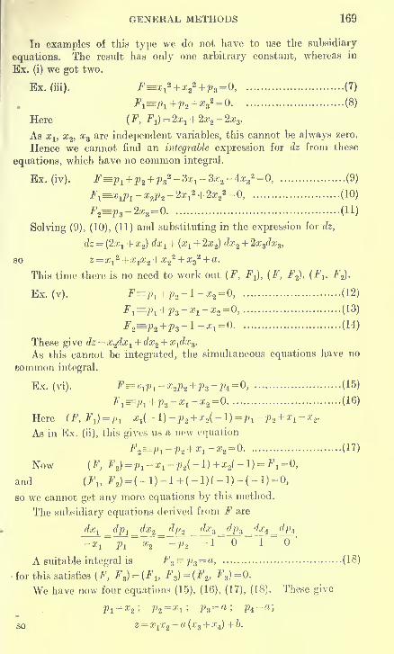
GENERAL METHODS 169
In examples of this type we do not have to use the subsidiary
equations. The result has only one arbitrary constant, whereas in
Ex. (i) we got two.
Ex. (iii). F=x x2 + x2
2 +p3 =0, (7)
Jispi+i>i +*,, -0 (8)
Here (F, FJ = 2xx + 2x2- 2x3 .
As xv x 2 , %3 are independent variables, this cannot be always zero.
Hence we cannot find an integrable expression for dz from these
equations, which have no common integral.
Ex. (iv). F=p1 +p 2 +p3
2 -3x1-3x 2 -ix3
2 = 0, (9)
Fl=x 1p 1-x2j) 2 -2x 1
2 + 2x22 = 0, (10)
F2=p 3 ~2x3=0. (11)
Solving (9), (10), (11) and substituting in the expression for dz,
dz = (2xt + x 2) dx x + (x
x+ 2x2) dx 2 + 2x3dx 3 ,
so z = x l2 + x
lx 2 + x 2
2 + x32 + a.
This time there is no need to work out (F, Fx),(F, F2), {Fx ,
F2).
Ex. (v). F=Pi +p 2-l-x2
= 0, (12)
F1=p l +p 3 -x 1-x2
= 0, (13)
F2=p2 +ps -l-x1=0 (14)
These give dz = xzdxx + dx2 + x xdx3 .
As this cannot be integrated, the simultaneous equations have no
common integral.
Ex. (vi). F=x1p x
-x2p 2 + p 3 -pi =0, (15)
F1=sp
l+ p 2 -x 1
-x2=:0 .....(16)
Here (F, Fl)=p 1-
x
1{-l)-p2 + x2{-l)=pl -p2 + x1-x2.
As in Ex. (ii), this gives us a new equation
F2=p 1
-p 2 + x1 -x 2=-0 (17)
Now (F, F2)=p 1 -x 1 -p 2
(-l)+x2(-l) = F 1=Q,
and (Fx , ig = (-l)-l+(-l)(-l)-(-l)=0,
so we cannot get any more equations by this method.
The subsidiary equations derived from F are
dx x dpx
dx2 _ dp 2_dx3 _dp 3 _dxi _dj)4
-xx
~p x
~
x
2 -p 2-1 1 6
A suitable integral is F3= p 3
= a, (18)
for this satisfies (F, F3 )= (FV F3 )
= (F2 , F3)=0.
We have now four equations (15), (16), (17), (18). These give
Pi = z2 ; P2= a;i; Vz = a "> V^ a '>
so z = x xx2 + a (x3 + :cd) + b.

170 DIFFERENTIAL EQUATIONS
But in this example we can obtain a more general integral. Thetwo given equations (15) and (16) and the derived one (17) are
equivalent to the simpler set
:
Vi=xz>' <19)
?2 = z,> (20)
?3-?4=0 (21)
From (19) and (20), z = xlx2 + a,ny function of x3 and x4 .
(21) is a linear equation of Lagrange's type, of which the general
integral is <}>(z, x3 + %i)=0,
i.e. z is any function of {x3 + x4), and may of course also involve a;,
and x2
.
Hence a general integral of all three equations, or of the two given
equations, is z= XyX ^ +^(^ + x^involving an arbitrary function. The complete integral obtained bythe other method is included as a particular case. The general integral
could have been obtained from the complete, as in Art. 134.
Examples for solution.
Obtain common complete integrals (if possible) of the following
simultaneous equations :
(1) Pl2+p 22-8(Xl + X2)2=0,
(p1 -p 2)(x1 -x2)+p3x3 -l=0.
(2) aj1apap8=3 ®2
aPaPi = a;3
27'iy2 = 1 -
(3) PiP^Pa- 8x^X3=0, (4) 2x3p1p3 -xipi = 0,'
p2 + p 3 -2x 2 -2x3=0. 2p t -p2
=0.
(5) pxx32 + p3 =0, (6) p 2
2 +p33 + x1 + 2x 2 + 3x3 =0,
p&a*+p&t* = p 1 +p42x4 -l=0.
(7) 2p 1 +p 2 +p3 + 2pi =0,
PlP3-P2?4=0.
(8) Find the general integral of Ex. (5).
(9) Find the general integral of Ex. (7).
MISCELLANEOUS EXAMPLES ON CHAPTER XIII.
(1) 2xyx3zp lp3 + x2p 2
= 0. (2) x2 p3 + x1pi =p 1p 3 -p 2p4 + x42 =0.
(3) 9x1xip1 (p 2 + p 3)-ip4
2 =0, (4) 9xlzp
1(p 2 + p3)-4:=0
)
p 1x 1 +p 2 -p3=0. PiXi+P2-Pa = Q-
(0) x1p 2p3 = x2p3p J—x3p^p2
= z x±x2x3 .
(6) p1z2 -x1
2=p2z2 -x 2
2 =p3z2 -x3
2 = 0.
(7) Find a singular integral of z —p lx 1 + p 2
x2 + p3x3 + p t
2 + p22 + p3
2,
representing the envelope of all the hyper-surfaces (in this case hyper-
planes) included in the complete integral.
(8) Show that no equation of the form F(xv x2 , x3 , pv p 2, p 3)=0has a singular integral.

Miscellaneous examples 171
(9) Show that if z is absent from the equation F{x, y, z, p, q)-0,Charpit's method coincides with Jacobi's.
(10) Show that if a system of partial differential equations is linear
and homogeneous in the p's and has a common integral
z = a 1u l + a 2u2 + ...
,
where the u'b are functions of the sc's, then a more general integral is
z = <t>(uv wa, ...)•
Find a general integral of the simultaneous equations
x1p1 -x2p2 + x2p3 =0,
xip3 -x^pi + x 5p b = 0.
(11) If p l and p 2 are functions of the independent variables xv x2
satisfying the simultaneous equations
F(xv x2 , pv p 2)=0 = F1 (x 1 , x2 , pv p 2),
proved (r.MkW^r-Hence 3how that if the simultaneous equations, taken as partial
differential equations, have a common integral, (F, Fx ) =0 is a necessary
but not a sufficient condition.
Examine the following pairs of simultaneous equations :
(i) 2^^ +2^-2 = 0,
2^(^+2^-1=0.d(F F-.)
CHere ~— = identically, and the equations cannot be solvedd(Vvlh)
\ for px and p 2.]
\(ii) F^Pl -p 2
* = 0,
\F1=p1 + 2pzx x
+x1i =0.
d(F F.)THere (F, F-.) and ^
—
'-—^ both come to functions which vanishd(Pv Vi)
when the p's are replaced by their values in terms of xx and x 2There
is no common integral.]
(iii) F=Pl -p 22 + x2 =0,
Fx^p x + 2^2^! + xx2 + x 2
=0.
d(F, F,)[These have a common integral, although _. - comes to a
d(Pi> P-i)
function that vanishes when the p's are replaced by their values.]

CHAPTER XIV
PARTIAL DIFFERENTIAL EQUATIONS OF THE SECONDAND HIGHER ORDERS
143. We shall first give some simple examples that can be
integrated by inspection. After this we shall deal with linear
partial differential equations with constant coefficients ; these are
treated by methods similar to those used for ordinary linear equations
with constant coefficients. The rest of the chapter will be devoted
to the more difficult subject of Monge's* methods. It is hoped that
the treatment will be full enough to enable the student to solve
examples and to make him believe in the correctness of the method,
but a discussion of the theory will not be attempted.!
Several examples will deal with the determination of the arbitrary
functions involved in the solutions by geometrical conditions. J
The miscellaneous examples at the end of the chapter contain
several important differential equations occurring in the theory of
vibrations of strings, bars, membranes, etc.
d2z d2z d2zThe second partial differential coefficients ^~v , - , ~~-% will
be denoted by r, s, t respectively.
144. Equations that can be integrated by inspection.
Ex. (i). s = 2x + 2y.
Integrating with resj)ect to x (keeping y constant),
q = x 2 + 2xy + e/)(y).
Similarly, integrating with respect to y,
z = x 2y + xy 2 + I (y) dy + f(.r),
say z = x2y + xy 2 +f (x) + F(y).
* Gaspard Monge, of Bcaune (1746-1818), Professor at Paris, created Descriptive
Geometry. He applied differential equations to questions in solid geometry.
t The student who desires this should consult Goursat, Sur Vintegration des
equations mix derivees partielles du second ordre.
X Frost's Solid Geometry, Chap. XXV., may be read with advantage.
172

SECOND AND HIGHER ORDERS 173
Ex. (ii). Find a surface passing through the parabolas
z = 0, y2 = iax and 2 = 1, y
z = -iax,
and satisfying xr + 2p=0.
The differential equation is
giving x2p=f(y),
z=-\f(y) + F{y).
The functions / and F are to be determined from the geometrical
conditions.
Putting 2 = and x = y2/ia,
Similarly l=~f(y) + F(y).
Hence F(y)J-, /(</)=£
and Z ~2 8acc'
i.e. 8a:r2: = 4ax - ?/2
, a conicoid.
Examples for solution.
(1) r = 6a;. (2) xys = l.
(3) £ = sina^/. (4) xr + p = 9x2y3
.
(5) 2/s +^> = cos (x + y) -y sin (» + ?/). (G) t-xq = x2.
(7) Find a surface satisfying s = 8xy and passing through the circle
z=0 = x2 + y2 -l.
(8) Find the most general conicoid satisfying xs + q = Ax + 2y + 2.
(9) Find a surface of revolution that touches 2 = and satisfies
r = 12x 2 + 4y 2.
(10) Find a surface satisfying t = 6x3y, containing the two lines
y = = z, y = \=z.
145. Homogeneous linear equations with constant coefficients. Tn
Chap. III. we dealt at some length with the equation
(Dn +a1Dn- 1 +a2D»-
2 + ... +an)y=f(x), (1)
where 7)=^-.ax

174 DIFFERENTIAL EQUATIONS
We shall now deal briefly with the corresponding equation in
two independent variables,
(Z>« + aJ)n-W + a2Dn-*D' 2 + ...+ anD'n
) z =f(x, y), (2)
where Z)e= — , D'==-
.
ox oy
The simplest case is (D - mD')z =0,
i.e. p-mq=0,
of which the solution is (p{z, y+mx) =0,
i.e. z=F(y +mx).
This suggests, what is easily verified, that the solution of (2)
iif{x,y)=0is
z =F1(y+ mp) +F2(y + m&) + ...+Fn (y +mnx),
where the %, m2 , ... mn are the roots (supposed all different) of
mn +a1mn-1 +a2mn~2 + ... +an =0.
3^z o z o z
dx? dx2 dy dxdy 2'
i.e. (Z)3 -3D 2Z)'+2DZ)' 2)2=0.
The roots of m3 -3m 2 + 2m=0 are 0, 1, 2.
Hence z = F1 (y) +
F
2 (y + x) +
F
3 (y + 2x).
Examples for solution.
(1) (IP-GDW + UDD' 2 -6D'3)z=0.
d 2z d 2z
(2) 2r + 5s + 2*=0. (3) g^-gp-0.
(4) Find a surface satisfying r + s = and touching the elliptic
paraboloid z = 4x 2 + y2 along its section by the plane y = 2x + 1 . [N. B.—
The values of p (and also of q) for the two surfaces must be equal for
any point on y = 2x + l.]
146. Case when the auxiliary equation has equal roots. Consider
the equation (D-mD') 2z=0 (1)
Put (D-mD')z=u.
(1) becomes (D -mD') w=0,
giving u=F(y + mx) ;
therefore (D -mD')z=F(y +mx),
or p-mq = F(y + mx).
The subsidiary equations are
dx _ dy dz
1 -m F(y+mx)'

SECOND AND HIGHER ORDERS 175
giving y +mx=a,
and • dz-F(a)dx=0,
i.e. z-xF (y + mx) = 6,
so the general integral is
<f>{z-xF(y+mx), y+mx}=0 or z=xF(y +mx) +Fx(y +mx).
Similarly we can prove that the integral of
(D-mD')nz=0
is z=xn~lF(y +mx) +xn~2F1(y +mx) + ... +Fn_1(y +mx).
Examples for solution.
(1) (4D2 + 12DD'+9D'2)z=0. (2) 25r-40s + 16t =0.
(3) (Z>»-4Z)aZ)'+4Z)Z)' a)2=0.
(4) Find a surface passing through the two lines 2 = 2 = 0,
2-1 =x-y=0, satisfying r-is + it =0.
147. The Particular Integral. We now return to equation (2) of
Art. 145, and write it for brevity as
F(D,D')z=f(x,y).
We can prove, following Chap. III. step by step, that the most
general value of z is the sum of a particular integral and the
complementary function (which is the value of z when the differ-
ential equation has /(a?, y) replaced by zero).
The particular integral may be written —^-r .f(x, y), and
we may treat the symbolic function of D and D' as we did that of
D alone, factorising it, resolving into partial fractions, or expanding
in an infinite series.
1 1 / 87)'\-2
E '9 ' D* -6DD' +9^, (12^+36^)=F>
(l --^-j (12tf + 36xy)
=F2 (1+^ +27^
2
+ -)' (12a;2 + 3G^ )
=- 2̂. (12a;2 + S6xy) +~ . 3Qx
= x4 + Qx?y + 9x4 = lOz4 + 6x3y,
so the solution of (D 2 - WD' + 9D' 2) z = l2x2 + S6xy
is 2 = 10a4 +6x3y + <p(y +3x) + x\Js(y +'3x).
Examples for solution.
(1) (D 2 -2DD' + D' 2)z = l2xy.
(2) {2D 2 -5DD' +2D' 2)z = 2i(y-x).

176 DIFFERENTIAL EQUATIONS
(3) Find a real function V of x and y, reducing to zero when y=0and satisfying
Q 2y ^ 2y_ + —„-4x<** + ,,*).
148. Short methods. When / (x, y) is a function of ax + by,
shorter methods may be used.
Now D(p (ax + by) = a<p' (ax + by) ; D'<f> (ax + by) = b<p' (ax + by).
Hence F (D, D') <j> (ax + by) =F (a, b)(f>
{n) (ax + by),
where<f>
{n)is the nth derived function of <j>, n being the degree of
F(D, D').
Conversely
F (D, U)^
(
aX + by^=Fja^b) $^ +^ (A)
provided F (a, 6)=/=0, e.g.
1 .„ „ >_ -sin(2a:+3y)
D*-4D*D' +4DD' 2°OS ^x+6y) ~2 3 -4 . 2 2
. 3 +4 . 2 .
3
2
= -32sin(2aj+3y),
since(f>
(2x + 3</) may be taken as - sin (2x + 3y) if
<p'" (2x +3y) =cos (2x +3y).
To deal with the case when F(a, b) = 0, we consider the equation
(D - mB') 2sp- mq = xr\fr(y + mx),
of which the solution is easily found to be
xr+l
so we may take
1 xr+1
D _mD > •
xr^(y + mx) =f+i^(y+™x).
Hence
t^ ^jz-\lr(v +mx) = -rF,„,.
,.x\}/(y +mx) = ...
(D-mD)nYKJ ' (D-mD) n-1 v XJ'
xn
=~,i'(y+mx)> (B
)
e '9 ' D2 -2DD , +D' 2tan (?/ +^ =^ tan ^ + ^'
while
D>-5DD' +W> Sin (4* + y)=irm D^D'
sin {ix +y)
=i) _ 4/)' • - 4 cos
(4x
+
y"> by (A)
= -\x cos (4a: + y) by (B).

SECOND AND HIGHER ORDERS 177
Examples for solution.
(1) (D2 -2DD' + D' 2)z = ex+ 2v.
(2) (D*-6DD' +9D' 2)z = 6x + 2y.
(3) (D^-4D 2D' + ±DD' 2)z=i sin (2x + y).
d 2V d2V(4) ar-.-ai-fc"/* (5) ^ + °^=l2(x + y)
(6) 4r-4s + « = 161og(a; + 2?/).
149. General method. To find a general method of getting a
particular integral, consider
(D -mD')z = p-mq=f(x, y).
The subsidiary equations are
dx _ dy _ dz
1~ -m~f(x, yY
of which one integral is y +mx=c.Using this integral to find another,
dz =/ (x, c - mx) dx,
z = I f(x, c-mx) dx + constant,
where c is to be replaced by y - mx after integration.
Hence we may take ^ jy .f(x, y) as I f(x, c -mx) dx, where
c is replaced by y + mx after integration.
Ex. (D-2D')(D + D')z = (y-l)e*.
Here \f{x, c-2x)dx=\ (c-2x-l)exdx= {c-2x + l)ex.
Therefore -=r
—
—=-, . (y - 1) ex = (y + 1) ex
, replacing c by y + 2x.
Similarly jr—=-, . {y + l)ex is found from I (c + x + l)exdx = (c + x)e*
by replacing c by y — x, giving yex, which is the particular integral
required.
Hence z=^yex + (p{y + 2x)+\fs(y -x).
Examples for solution.
(1) (D 2 + 2DD' + D' 2)z = 2cosy-XKh\y.
(2) (D 2 -2DD' -WD' 2)z = 12xy. (3) (r + s-Gt)z = y cos x.
(4) ^-^- 2^ =^ + ^-y«)8m^-co8^.
(5) r-t = tan3 x tan y - tan x tan3?/.
{' dx2 dt 2
t2 x2
'
P.D.E. M

178 DIFFERENTIAL EQUATIONS
150. Non-homogeneous linear equations. The simplest case is
(D-mD' -o)2=0,
i.e. p -mq = az,
giving <p (ze~ax,y+mx) =0,
or z=eax\fs(y +mx).
Similarly we can show that the integral of
(D-mD' -a)(D-nD' -b)z=0is z=eaxf(y+mx)+ebxF(y+nx),
while that of (D - mD' - afz =
is z=eaxf(y+mx)+xeaxF(y+mx).
But the equations where the symbolical operator cannot be
resolved into factors linear in D and D' cannot be integrated in this
manner.
Consider for example (D2 -D')z=0.
As a trial solution put z = e1uc+ky
,giving
{D2 -D')z = (h2 -k)e'"+ki>.
So z=eh{x+hy)is a particular integral, and a more general one is
YlAeh(xJrliy\ where the A and h in each term are perfectly arbitrary,
and any number of terms may be taken.
This form of integral is best suited to physical problems, as was
explained at some length in Chap. IV. Of course the integral of
any linear partial differential equation with constant coefficients
may be expressed in this manner, but the shorter forms involving
arbitrary functions are generally to be preferred.
Examples for solution.
(1) DD'(D-2D' -3)2 = 0. (2) r + 2s + t + 2p + 2q + l=0.
(3)li* Tt-
(4) (D2 - I)
'2+I) - I) ') z = -
d 2V d 2V(5) (2D4-3D 2 Z)' + Z)'
2)z=0. (6) ^T+^F=» 2^
(7) (Z)-2D'-l)(Z>-2Z>' 2 -l)z = 0.
(8) Find a solution of Ex. (4) reducing to 1 when x= +00 and to
?/2 when x = 0.
151. Particular Integrals. The methods of obtaining particular
integrals of non-homogeneous equations are very similar to those in
Chap. III., so we shall merely give a fewT examples.
Ex. (i). (IP-3DD' + D + l)z = e 2*+sy,
i r 2x+3y
e2x+3?/ = = _ l_e2x+Sy
Pi -3DD' + D + ]
'
23 -3.2.3+2 + l

SECOND AND HIGHER ORDERS 179
Hence z = - }e2x+3v + lAe hx+k^,
where h* - 3hk +h + 1 =0.
Ex. (ii). (D + D'-l){D + 2D'-3)z = 4: + 3x + 6y.
= i{l + D + D' + terms of higher degree}
( D + 2D' . L ., J )x
11 H 1- terms of higher degree
J-
. j. 4D + 5Z)' ... , , )= -g- 1 1 H h terms of higher degree j-.
Acting on 4 + 3x + 6y, this operator gives
${4+3x +6y+4: + 10}=>6 + z+ 2y.
Hence z = 6 + x + 2y + exf (y-x) + e3xF(y - 2x).
Ex. (Hi). (Z) 2 - DD f - 2D) z = sin (3x + 4y).
D 2 -DD'-2D •Sin (3* + 4y) = -32-(-3.4)-2D ' "^ f^ + iy)
=3^2^* sin(3aJ + 4^
_ 3 + 2J 3 sin (3s + 4y) + 6 cos (8s + 4y)-9T4^- sin(,3a; + 4^-~
9 -4(-3 2)
= TV sin (3x + 4t/) + T2s cos (3a; + 4y).
Hence z = TV sin (3x + ±y)+-h cos(3a; + 42/) + 2J^
e
te+ A'y,
where h 2 -hk-2h=0.
Examples for solution.
(1) (D- D' -l)(D- D' -2)z = e**-v.
(2) s +p-q = z + xy. (3) (D- D' 2)z = cos (x-3y).
(4) r-s+p-l. (5) g-g^-f-^*.
(6) (Z)-3Z)'-2) 2z = 2e 2*tan(2/ + 3a;).
152. Examples in elimination. We shall now consider the result
of eliminating an arbitrary function from a partial differential
equation of the first order.
Ex. (i). 2px-qy = <p(x 2y).
Differentiating partially, first with respect to x and then toy/, we get
2rx -sy + 2p = 2xyqy'(x2y),
and 2sx-ty-q = x2(/)'(x
2y),
whence x(2rx -sy + 2p) = 2?/(2s:r -ty-q)
or 2x 2r - 5xys + 2y 2
t + 2 {px + qy) = 0,
which is of the first degree in r, s, t.

180 DIFFERENTIAL EQUATIONS
The same equation results from eliminating \fs from
px-2qy = \fs(xy2).
Ex. (ii). p2 +q= <j>{2x + y).
This gives 2pr + s = 2<p'{ 2x + y),
and 2ps + t = <p'(2x + y),
whence 2pr + s = ips + 2t,
again of the first degree in r, s, t.
Ex. (iii). y-p = <p(x-q).
This gives -r = (l -s)cp'(x-q),
and - l-s= -t<f>'(x-q),
whence rt = (l-s) 2
or 2s + (rt-s 2) = l.
This example differs from the other two in that p and q occur inj
the arbitrary function as well as elsewhere. The result contains a
term in (rt - s 2)
Examples for solution.
Eliminate the arbitrary function from the following :
(1) py-q + 3y 2 = (j>(2x + y2). (2) x-- = q>(z).
(3) p + x-y = <p(q-2x + y). (4) px + qy = (f>(p2 + q
2).
(5) p2 -x = <p(q
2 -2y). (6) p+zq = <p(z).
153. Generalisation of the preceding results. If u and v are
known functions of x, y, z, p, q, and we treat the equation u =(J>
(v)
as before, we get
du du du du ( dv dv dv dv\ .. .
, du du du du ( dv dv dv dv\ .. .
and ^V^a^l^VaT/^l)-^"'-Eliminating <j)'(v) we find that the terms in rs and st cancel out,
leaving a result of the form
Rr+Ss+Tt + U(rt-s2) = V,
where R, S, T, U and V involve p, q, and the partial differential
coefficients of u and v with respect to x, y, z, p, q.
„ du dv dv duThe coefficient u = =- _— , - ~-
,
dp dq dp oq
which vanishes if v is a function of x, y, z only and not of p or q.
These results will show us what to expect when we start with
the equations of the second order and try to obtain equations of the
first order from them.

SECOND AND HIGHER ORDERS 181
154. Monge's method of integrating Rr + Ss+Tt=V. We shall
now consider equations of the first degree in r, s, t, whose coefficients
R, S, T, V are functions of p, q, x, y, z, and try to reverse the process
of Arts. 152 and 153.
Since dp = * dx + ^ dy = rdx+sdy
and dq=sdx+tdy,
Rr+Ss+Tt-V=0
becomes *(&-"£*) + Ss +t(*^) -7-0,
i.e. Rdpdy + T dqdx -V dy dx -s (R dy2 -S dy dx + T dx2) =0.
The chief feature of Monge's method is obtaining one or two
relations between p, q, x, y, z (each relation involving an arbitrary
function) to satisfy the simultaneous equations
Rdy2 -Sdydx + Tdx2 =0,
Rdpdy + T dqdx- V dy dx =0.
These relations are called Intermediate Integrals.
The method of procedure will be best understood by studying
worked examples.
Ex. (i)
.
2x2r - 5xys + 2yH + 2 (px + qy) = 0.
Proceeding as above, we obtain the simultaneous equations
2x2 dy2 + 5xydydx + 2y 2 dx2 =0, (1)
and 2x2 dpdy + 2y 2 dqdx + 2{px + qy)dydx = (2)
(1 ) gives (x dy + 2y dx) (2xdy + y dx) = 0,
i.e. x2y — a or xy2 = b.
If we take x2y = a and divide each term of (2) by xdy or its equivalent
-2ydx, we get 2xdp-ydq + 2pdx-qdy=0,
i.e. 2px — qy = c.
This, in conjunction with x2y = a, suggests the intermediate integral
2px-qy = <f>(x2tj), (3)
where <j> is an arbitrary function. [Cf. Ex. (i) of Art. 152.]
Similarly xy2 = b and equation (2) leads to
px-2qy = \p-{xy 2) (4)
Solving (3) and (4),
3px = 2<p{x2y)-\l,{xy2),
3qy = (t>{x2y)-2\Js{xy 2
),

182 DIFFERENTIAL EQUATIONS
so dz = pdx + qdy = i<l>(x?y).(^ +^)-^(xy2).^ +~^y
i.e. z =^<p {xhj) . d log {x2y) - ij ^ (xy 2) . d log {xy2
),
or z=f(x2y) + F{xy 2
).
Ex. (ii). y2r-2ys + t=p + 6y.
Eliminating r and t as before, we are led to the simultaneous equa-
tionsij2 dy2 + 2ydydx + dx2 =0, (5)
and y2 dp dy + dq dx - (p + 6y) dy dx =0 (6)
(5) gives {ydy + dx) 2 =0,
i.e. 2x + y2 = a.
Using this integral and dividing each term of (6) by y dy or its
equivalent - dx, we get
ydp-dq + (p + 6y)dy=0,
i.e. py - q + Sy 2 = c.
This suggests the intermediate integral
py-q+3y2 = <p(2x + y2).
As we have only one intermediate integral, we must integrate this
by Lagrange's method.
The subsidiary equations are
dx dy dz
i;=~l
=:
-3y2 + <t>(2x + y2)'
One integral is 2x + y2 = a. Using this to find another,
dz + {-3y 2 + <j>(a)}dy = 0,
i.e. z-yz + y<j>{2x + y2)=b.
Hence the general integral is
yf,{z-f + y<p(2x + y2), 2x + y
2}=0,
or z — y*-y<f>(2x + y2)+f(2x + y
2).
Ex (iii). pt-qs^q*.
The simultaneous equations are
qdydx+pdx2 =0, (7)
and pdqdx-q3 dydx=0 (8)
(7) gives dx=0 or qdy + pdx(=dz)—0,
i.e. x = a or z = b.
If dx = (8) reduces to 0=0.If z = b, qdy= -pdx and (8) reduces to
pdq + q2p dx = 0,
i.e. dq/q2 + dx=0,
giving -- + x = c = \fr(z) (9)

SECOND AND HIGHER ORDERS 183
(9) may be integrated by Lagrange's method, but a shorter way is
to rewrite itfiv \
giving y = xz- I \fs(z)dz + F(x)
y = xz+f(z) + F(x).
Examples for solution.
(1) r— l cos 2 x + p tan x=0.
(2) (x - y) {xr -xs-ys + yt) =(x+ y) (p - q).
(3) (q + l)s = (p + l)t. (4) t-rscc*y = 2qtany.
(5) xy(t-r) + (x2 -y 2)(s-2)=py- qx.
(6) (l+q) 2r-2(l+p + q + pq)s + (l+p) 2t=0.
(7) Find a surface satisfying 2x 2r-5xys + 2yH + 2(px + qy) =0 and
touching the hyperbolic paraboloid z = x2 -y 2 along its section by the
plane y = 1
.
(8) Obtain the integral of q2r-2pqs+pH = in the form
y + xf(z) = F(z),
and show that this represents a surface generated by straight lines that
are all parallel to a fixed plane.
155. Monge's method of integrating Rr +Ss +Tt +U(rt-s 2) V.
As before, the coefficients R, S, T, U, V are functions of p, q,
x, y, z.
The process of solution falls naturally into two parts :
(i) the formation of intermediate integrals ;
.
(ii) the further integration of these integrals.
For the sake of clearness we shall consider these two parts
separately.
156. Formation of intermediate integrals. As in Art. 154,
r = {dp - s dy)/dx
and t = (dq-s dx)/dy.
Substitute for r and &'m
Rr+Ss + Tt + U{rt-s2)= V,
multiply up by dx and dy (to clear of fractions), and we get
R dp dy + Tdqdx + U dp dq - V dx dy
-s(R dy2 -Sdxdy + Tdx2 + U dp dx + U dq dy) = 0,
say M -sN=0.* The remainder of this chapter should be omitted on a first reading. This
extension of Monge's ideas is due to Andre Marie Ampere, of Lyons (1775- 1830),
whose name has been given to the unit of electric current.

184 DIFFERENTIAL EQUATIONS
We now try to obtain solutions of the simultaneous equations
M=0,N=0.
So far we have imitated the methods of the last paragraph, but
we cannot now factorise N as we did before, on account of the
presence of the terms U dpdx + U dq dy.
As there is no hope of factorising M or N separately, let us try
to factorise M+XN, where X is some multiplier to be determined
later.
Writing M and N in full, the expression to be factorised is
Rdy2 +T dx2 -{S +XV)dxdy + U dpdx + U dq dy
+XRdp dy +XT dq dx+XU dp dq.
As there are no terms in dp2 or dq2, dp can only appear in one
factor and dq in the other.
Suppose the factors are
Ady+Bdx+C dp and Edy+Fdx+Gdq.Then equating coefficients of dy2
, dx2, dp dq,
AE = R; BF = T; CG=XU.We may take
A=R, E = l, B = kT, F = l/k, C = mU, G = X/m.
Equating the coefficients of the other five terms, we get
JcT+R/k= -(S+XV), (1)
XR/m = U, (2)
JcTX/m=XT, (3)
mU=XR, (4)
mU/k = U (5)
From (5), m = k, and this satisfies (3).
From (2) or (4), m = XR/U.
Hence, from (1),
X 2 (RT + UV)+XUS + U2 =0 (6)
So if A is a root of (6), the factors required are
(Rdy+X y-j dx +XR dp) (dy + w-, dx + p dq),
7? 1
i.e. j-j (U dy +XT dx +XU dp) .^ Q^R dy + U dx+XUdq).
We shall therefore try to obtain integrals from the linear
equations U dy +XT dx +XU dp =0 (7)
and XRdy + Udx+XUdq=0, (8)
where X satisfies (6).

SECOND AND HIGHER ORDERS 185
The rest of the procedure will be best understood from worked
examples.
157. Examples.
Ex. (i). 2s + (rt-s*)=*l.
Substituting R=T = 0, S=2, £/=F=l in equation (6) of the last
article,* we get \2 + 2\ + 1 = 0,
a quadratic with equal roots -1 and -1.
With X= -1, equations (7) and (8) give
dy — dp = 0,
dx-dq — 0,
of which obvious integrals are
y —p = const,
and x - q = const.
Combining these as in Art. 154, we get the intermediate integral
y-p=f{x-q).
Ex. (ii). r + 3s*+t + {rt-s2)=>l.
The quadratic in X comes to
2X 2 + 3X + 1=0,so X = - 1 or - 1
.
With X= -1, equations (7) and (8) give
dy-dx-dp=0,
-dy + dx-dq =0,
of which obvious integrals are
p + £-?/= const (1)
and q-x + y = const (2)
Similarly X = - J leads to
p + x-2y = comt. (3)
and 9 -2a; +y= const (4)
In what pairs shall we combine these four integrals ?
Consider again the simultaneous equations denoted by M=0, N =in the last article. If these are both satisfied, then M + X 1
iV = and
M + \ 2N =0 are also both satisfied fwhere X x
and X 2are the roots of the
quadratic in X). Therefore one of the linear factors vanishes for X = X,
and one (obviously the other one, or else dy = 0) for X = X 2.
That is, we combine integrals (1) and (4), and also (2) and (3),
giving the two intermediate integrals
p + x-y=f(q-2x + y)
and p + x - 2y = F(q - x + y).
* We quote the results of the last article to save space, but the student is
advised to work each example from first principles.

186 DIFFERENTIAL EQUATIONS
Ex. (iii). 2yr + (px + qy)s + xt- xy(rt - s2) = 2 - pq.
The quadratic in X comes to -
X 2xypq - \xy (px + qy)+ x2y2 = 0,
giving X = y/P or x/q.
Substituting in (7) and (8) of the last article, we get, after a little
reduction, pdy-dx + ydp=Q, (5)
2y dy - px dx - xy dq=0, (6)
- qy dy + x dx - xy dp = 0, (7)
and -2dy + qdx + xdq=0 (8)
Combining the obvious integrals of (5) and (8), we get
yp-x=f(-2y+ qx).
But (6) and (7) are non-integrable. This may be seen from the
way that p and q occur in them. Thus, although the quadratic in X has
two different roots, we get only one intermediate integral.
Examples for solution.
Obtain an intermediate integral (or two if possible) of the following :
(1) 3r + is + t + (rt-s 2)=l. (2) r + t-(rt-s2)=l.
(3) 2r + tex -(rt-s 2)=2ex. (4) rt-s2 + 1=0.
(5) 3s + (rt-s 2) =2.
(6) qxr + (x + y) s + pyt + xy (rt - s 2) = 1 - pq.
(7) (q2 - 1) zr - 2pqzs + (p
2 -l)zt + z2 (rt - s 2) = p 2 + q2 - 1
.
158. Further integration of intermediate integrals.
Ex. (i). Consider the intermediate integral obtained in Ex. (i) of
Art. 157, y_2i=f(x-q).
We can obtain a " complete " integral involving arbitrary constants
a, b, c by putting x-q = a
and y - p =f (a) = b, say.
Hence dz =p dx + q dy = (y -b) dx + (x- a) dy
and z=xy- bx - ay + c.
An integral of a more general form can be obtained by supposing
the arbitrary function / occurring in the intermediate integral to be
linear, givingy_ p = m (x - q)+ n .
Integrating this by Lagrange's method, we get
z = xy + <p(y + mx) - nx.
Ex. (ii). Consider the two intermediate integrals of Ex. (ii), Art. 157,
p + x-y=f(q-2x + y)
and p + x-2y = F(q-x + y).

SECOND AND HIGHER ORDERS 187
If we attempt to deal with these simultaneous equations as we dealt
with the single equation in Ex. (i), we get
q - 2x + y = a,
q-x+y=fi,
p + x-y=f(a),
p + x-2y = F(j3).
If the terms on the right-hand side are constants, we get the absurd
result that x, y, p, q are all constants !
But now suppose that a and /3 are not constants, but parameters,
capable of variation.
Solving the four equations, we get
x = (5-a,
V-f(a)-F(fap = y-x+f(a),q=, x -y + (3,
giving dz=pdx + qdy= (y-x) (dx - dy) +f (a) dx + (3 dy
= - \d {x - y)* +/(a) d(3 -/(a) da + fif'(a) da - fiFtf) d/3 :
i.e. z =-l(x-y)2-^f(a)da-^F'(p)dp + Pf(a).
To obtain a result free from symbols of integration, put
( f(a)da = <j>(a) and f F(/3) rf/3 =^ ((3).
Now [ @F'(p) d/3 - f3F{(3) - \F(/3) d/3, integrating by parts,
= /3V/(/3)-V'(/3)
Hence z = - £ (x - yf -<f>
(a) - /3y/(/3) + ^ (/3) + /3<p'(a),
rz=-h(x-y) 2 -<p(a) + ^( l8)+(3y,
or finally j x = /3 - a,
These three equations constitute the parametric form of the equation
of a surface. As the solution contains two arbitrary functions, it maybe regarded as of the most general form possible.
Examples for solution (completing the solution of the preceding set).
Integrate by the methods explained above :
(1) p +x-2y=f{q-2x + 3y). (2) p-x=f(q-y).
(3) p-e*=f{q-2y). (4) p-y=f(q + x),
p + y = F(q-x).
(5) P-V =/ (q - 2s), (6) px - y =f (qy- x).
p-2y = F(q-x). (7) (zp-x)=f(zq-y).
(8) Obtain a particular solution of (4) by putting 0(a)=-£a 2,
\fr ((3) = 1/32 and eliminating a and (3.

188 DIFFERENTIAL EQUATIONS
MISCELLANEOUS EXAMPLES ON CHAPTER XIV.
(1) r = 2y2. (2) log s = x + y. (3) 2yq+y*t = l.
(4) r-2s + t = sm{2x + 3y). (5) x2r-2xs + t + q=0.
(6) rx2 -3sxy + 2ty2 +px + 2qy = x + 2y.
(7) y2r + 2xys + x2
t + px + qy = 0.
(8) 5r + Gs + 3t + 2(rt-s2)+3 = 0.
(9) 2pr + 2ql-4:pg(rt-s 2) = l.
(10) rt - s 2 - s (sin a; + sin y) = sin x sin */.
(11) 7r-8s-3i + (rt-s 2)=36.
(12) Find a surface satisfying r = 6x + 2 and touching z = x3 + y3
along its section by the plane x + y + 1 = 0.
(13) Find a surface satisfying r-2s + t = 6 and touching the hyper-
bolic paraboloid z = xy along its section by the plane y = x.
(14) A surface is drawn satisfying r + l = and touching x2 + z2 — l
along its section by y=0. Obtain its equation in the form
z 2 (x 2 + z 2 -l) = y2 (x2 + z 2). [London.]
(15) Show that of the four linear differential equations in x, y, p, qobtained by the application of Monge's method to
2r + qs + xt - x (rt - s 2) = 2,
two are integrable, leading to the intermediate integral
P-x=f(qx-2y),while the other two, although non-integrable singly, can be combined
to give the integral?, + J?
2 _ x = a>
Hence obtain the solutions
z = \x 2 - 2mxy - fmPx3 + nx + <p(y + hnx2
)
and z = (a- \h 2)x + \x2 + by + c,
and show that one is a particular case of the other.
(16) A surface is such that its section by any plane parallel to x=0is a circle passing through the axis of x. Prove that it satisfies the
functional and differential equations
y2 + z 2 + yf(x)+zF(x)=0,
(y2 + z 2)l + 2(z-yq)(l+q 2)=0.
(17) Obtain the solution of x 2r + 2xys + y2t = in the form
*=/(!)^(f>and show that this represents a surface generated by lines that intersect
the axis of z.
(18) Show that rt-s 2 = leads to the " complete " integral
z = ax + by + c.

MISCELLANEOUS EXAMPLES 189
Show that the " general " integral derived from this (as in Art. 134)
represents a developable surface (see Smith's Solid Geometry, Arts.
222-223).
Hence show that for any developable surface q=f(p).
(19) Find the developable surfaces that satisfy
pq(r -t)- (p2 -q 2)s + {py - qx) (rt - s 2) =0.
[Assume q =/(/>). This is called Poisson's method. We get
q = ap or p2 + q
2 = b2,
giving z = <p(x + ay) or z = bx cos a + by sin a + c.
The second of these integrals represents a plane which generates the
developable surface given by the corresponding " general " integral.]
(20) Show that if
X=p, Y = q, Z=px + qy-z,
then r=TJ(RT-S 2), s= -S/(RT-S 2
), t = R/(RT-S 2),
where R = ^y^, etc.
Hence show that the equation
ar + bs + ct + e (rt - s 2) =
transforms into AT - BS + CR + E = 0,
where a, b, c, e are any functions of x, y, p, q, and A, B, C, E the corre-
sponding functions of P, Q, X, Y.
Apply this Principle of Duality (cf. No. 21 of the Miscellaneous
Examples at the end of Chap. XII.) to derive two intermediate integrals
°f pq(r -t)- (p2 -q 2)s + (py - qx) (rt - s2) =0.
(21) Prove that if x, y, u, v are real and u + iv=f(x + iy), then F = ?t
and V — v are both solutions of
d 2V dWdx 2 dy2 '
and the two systems of curves a = const.,
v= const.,
are mutually orthogonal.
Verify these properties for the particular cases
(i) u + iv = x + iy,
(ii) u + iv= (x + iy) 2,
(iii) u + iv = ]((x + iy).
[The differential equation is the two-dimensional form of La place's
equation, which is of fundamental importance in gravitation, electro-
statics and hydrodynamics, u and v are called Conjugate Functions.
See Ramsey's Hydro-Mechanics, Vol. II. Art. 11.
J
(22) Obtain the solution of
a 2// J^y
dt 2 """dx 2'

190 DIFFERENTIAL EQUATIONS
subject to the conditions y=f(x) and ~ = F(x) when «=0, in the form
1 Cx+at
y = U(x + at) + $f(x-at) + -\ F(\)d\.taJx-at
[y is the transverse displacement of any point x of a vibratingstring of infinite length, whose initial displacement and velocity are
given by f(x) and F(x). See Ramsey's Hydro-Mechanics, Vol. II.
Art. 248.]
(23) If y=f(x) cos (nt + a) is a solution of
dt 2+(l
d*4~U
'
show that f(x)=A sin mx + B cos mx + H sinh mx + K cosh mx, where
m = \/(n/a 2).
[The differential equation is that approximately satisfied by thelateral vibrations of bars, neglecting rotatory inertia. See Rayleigh's
Sound, Art. 163.]
(24) Show that
w = A sin (mirx/a) sin (mry/b) cos {pet + a)
,. a d 2w vfdhv d 2w\satafies W=°\w +
W>'and vanishes when
a:=0, y = 0, x = a or y = b,
provided that m and n are positive integers satisfying
(p/7r)2 = (m/a) 2 + (w/6) 2
.
[This *gives one solution of the differential equation of a vibrating
membrane with a fixed rectangular boundary. See Rayleigh's Sound,Arts. 194-199.]
(25) Show that w=AJ {nr) cos (nct + a)
,. o d 2w /d 2w 1 dwSatlsfi6S
"
Tt2^ C
\ji2+ rTrwhere J is Bessel's function of order zero (see Ex. 2 of the set following
Art. 97).
[This refers to a vibrating membrane with a fixed circular boundary.
See Rayleigh's Sound, Arts. 200-206.]
(26) Show that V = (Arn + Br-"-1) Pn (cos 6)
. _ a 2F 2 3F i dw cot oarrt
where P„ is Legendre's function of order w (for Legendre's equation,
see Ex. 2 of the set following Art. 99).
[N. B.—Take /j. = cos 6 as a new variable. This equation is the
form taken by Laplace's potential equation in three dimensions, whenV is known to be symmetrical about an axis. See Routh's Analytical
Statics, Vol. II. Art! 300.]

APPENDIX A
The necessary and sufficient condition that the equation M dx + N dy =should be exact
(a) If the equation is exact,
M dx +N dy = a, perfect differential = df, say.
So M =% and N =% >
- dx oy
it . dN a 2/ d 2f bm
therefore — = —-;- =—i- =—-
,
ox oxoy oyox oyso the condition is necessary.
(6) Conversely, if — =—,put F=\Mdx, where the integration
is performed on the supposition that y is constant.
„, dF __ d 2F d 2F dM BNIhen -=- =M and - - = =—=- = -=- = -=-
.
ox oxoy oyox oy ox
* £(*-$-*
N - -=— = a constant as far as a; is concerned, that is,
J a function of y,
= 0(y)»say.
Then iV =^ + 0(y).
Now put /= F + I («/) %.
Then N = %£.oy
dFAlso M = -=- by definition of F
ox
= 4~, since F and /differ only by a function of y.
Thus M dx + N dy = ~- dx + ~- dy = df, a perfect differential.
So the equation is exact, that is, the condition is sufficient.
d 2f d 2
f
~~~*
[Our assumption that =—~ = ~—"i is justified if / and its first and
second partial differential coefficients are continuous. See Lamb's
Infinitesimal Calculus, 2nd ed., Art. 210.]
191
APPENDIX B
The equation P(x, y, z) ~- +Q(x, y, z) —- + R(x, y, z)~ = 0, regarded as
four-dimensional, has no special integrals. (See Art. 127.)
Let u(x, y, z)=a,
v(x, y, z) = b,
be any two independent integrals of the equations
dx/P = dy/Q = dz/R.
Then we easily prove that
du Bu du _ .,
.
PS-X+Q
di+ R
S-z=° (1)
and p^ +Q f_ +B 3jl _ (2)Bx By Bz
The left-hand side of (1) does not contain a, and therefore cannot
vanish merely in consequence of the relation u = a. Hence it mustvanish identically. Similarly equation (2) is satisfied identically.
Now let f=w(x, y, z) be any integral of the original partial
differential equation, so that
n Biv „Bw n Bw _ /0 ,P8^
+QSlj
+Rdi
=<> (3)
This is another identical equation, since / does not occur in it.
Eliminating P, Q, R from (1), (2), (3), we get
^4=0 identically.B(x,y,z)
Hence w is a function of u and v, say
W = (f)(u, v).
That is, /=w is part of the General Integral, and therefore, as /=wis any integral, there are no Special Integrals.
[The student will notice the importance in the above work of a
differential equation being satisfied identically. Hill's new classification
of the integrals of Lagrange's linear equation (Proc. London Math. Soc.
1917) draws a sharp distinction between integrals that satisfy an
equation identically and those which have not this property.]
192

APPENDIX
The expression obtained for dz by Jacobi's method of solving a single
partial differential equation of the first order (Art. 140) is alwaysintegrable.
To prove that dz =pxdxx + p 2dx2 + p3dx3
is integrable it is necessary and sufficient to prove that
L =M = N=0, (A)
where iJ^-^, mJ^-^, nJ^-^.OX3 OX2 OXy ox3 ax2 ox
l
Now, by adding equations (8), (9), (10) of Art. 140 and using the
relation (F, Fl ) = 0, but not assuming the truth of (A), we get
I'gilA +MWfi +s'JL3i =0 (B,o(Pt, Ps) o(p3 , px) d(pv p2)
a . ., . T d{Fv F2 ) ..d(Fv Fi) .Td(Fv F2 ) _
Similarly L -^—^—^ +M^-^—% + N-±-J>—^=0 (C)oiPvto) °iPz>Pi) d(pv p2)
T d(F2) F) .,d(F 2,F) „d(F2,F) nand £ a ;
8; +M ~-2
—
[ +N~^— =0 (D)o(p 2 , Pz) o{p 3 , p x ) d(plt p 2 )
From equations (B), (C), (D) we see that either L —M=N—0 or
A = 0, where A is the determinant whose constituents are the
coefficients of L, M, N in (B), (C), (D).
But these coefficients are themselves the co- factors of the constituents
of the determinant a/ ™ w p \
~d(Pi>P2>Ps)'
and by the theory of determinants A=«72-
Now J cannot vanish,* for this would imply the existence of a
functional relation which would contradict the hypothesis of Art. 140
that the p's can be found as functions of the as's from
F=F1 -a i= F2 -a 2
= 0.
Hence A^0; therefore L =M = N = 0.
* All the equations of this appendix are satisfied identically.
193

APPENDIX D
Suggestions for further reading
No attempt will be made here to give a complete list of works ondifferential equations. We shall merely give the names of a very
small number of the most prominent, classified in three sections.
I. Chiefly -of analytical interest (forming a continuation to Chapter X.).
(a) Forsyth : Theory of Differential Equations (1890 and later years,
Cambridge Univ. Press).
This important work is in six volumes, and is the most exhaustive
treatise in English upon the subject. It should not be confused with
his more elementary work in one volume (4th ed. 1914, Macmillan).
(b) Goursat : Cours d'Analyse matMmatiqne, Vols. II. and III. (2nd
ed. 1911-15, Gauthier-Villars ; English translation published by Ginn).
This deals almost entirely with existence theorems.
(c) Schlesinger : Handbuch der Theorie der linearen Differential-
gleichungen (1895-8, 3 vols, Teubner).
II. Partly analytical but also of geometrical interest.
(a) Goursat : Equations aux dirivies partielles du premier ordre (1891).
(b) Goursat : Equations anx de'rive'es partielles du second ordre
(1896-98, 2 vols., Hermann et fils).
(c) Page : Ordinary differential equations from the standpoint of Lie's
Transformation Groups (1897, Macmillan).
This deals with the elements of differential equations in a highly
original manner.
III. Ofphysical interest (forming a continuation to Chapters III. and IV.).
(a) Biemann : Partielle Differentialgleichungen und deren Anwendungauf physikalische Fragen (1869, Vieweg).
(b) Riemann-Weber : A revised edition of (a), with extensive
additions (1900-01, Vieweg).
(c) Bateman : Differential Equations (1918, Longmans).This contains many references to recent researches.
It is impossible to mention original papers in any detail, but the
recent series of memoirs by Prof. M. J. M. Hill in the Proceedings of tlie
London Mathematical Society should not be overlooked.
194

MISCELLANEOUS EXAMPLES ON THE WHOLE BOOK
. dy ^y* + 2,x 2yy () dx~a? + 3xyf [London.]
? (2) £ + ^V = 2« (1 + a2). [London.
]
>(3) tan ?/ ^ + tan a; = cos y cos3z. [London.]
(4) ^ 2*i + (!)
2
London.]
(5) (1 -x2)-£-xy = x 2y2. [London.]
(6) (Z>2 + 4)*/ = sin2z. [London.]
(7) (D3 -D 2 + 3D + 5)y = x2 + e*cos2x. [London.]
(8) (x3D3 + x 2D 2)y = l+x + x 2. [London.]
/«» • dy(9) cos x sin cc -— = y + cos x. [London.]
[London.]
(10) ^-= » + y + 2cos«,-
dt~6x y -
(11) ^/= a;
(^)
3
+ l- [London.]
(13) (D4 +8D2 + 16)?/ = a;cos2a:. [London.]
(14) I x2dy+ I xydx = x3 . [London.]
(15) (?/2 + yz - z) dx + (x 2 + xz - z) dy + (x + y- xy) dz = 0. [London
.
]
(16) (2x* - y3 - z3
)yz dx + (2y
3 - z3 - x3) zx dy + (2z3 - x3 - y
3) xy dz = 0.
[London.]
(17) xp-yq + (x 2 -y 2)=0. [London.]
(18) (x + 2y -z)p + (3y-z)q = x + y. [London.]
195

.2
196 DIFFERENTIAL EQUATIONS
/.^v 2 (xz - yz + xy) _ _ , ,(19) xp + yq+ \
3
X + Z=0 ' London.]
(20) p(x + p)+q(y + q) = z. [London.]
(21) r + s=p. [London.]
(22) z-\px-qy=p2\x2. [London.]
(23) r-x = t-y. [London.]
(24) z = px + qy-sxy. [London.]
(25) z \rt - s 2) + pqs = 0. [London. ]
(26) x2r + 2xys + y2t = xy. [London.]
(27) rq(q + l)-s(2pq+p + q + l)+tp(p + l)=0. [London.]
(28) y3 =xy 2p + x*p 2
. [Math. Trip.]
(30) Pi - -i?- + x2ny=0. [Math. Trip.]
ax2 x ax
(31) (zp + x) 2 + (zq + ij)2 = l. . [Math. Trip.]
(f2y dy
(32) Find a solution of the equation j\- 3 — + 2y = e3x which shall
vanish when x=0 and also when x = loge2. [Math. Trip.]
(33) Solve the equation
d oc doc
-j-£ + 2k-j-+ (k2 + \ 2)x = A cos pt.
Show that, for different values of p, the amplitude of the particular
integral is greatest when p2 = \ 2 -K 2
, and prove that the particular
integral is then
(A/2k\) cos (pt - a), where tan a =p/k. [London.]
(34) Solve the equation
d2v dy o
T^ + ~r tanaj + tycos-x =dxl ax
by putting z = sin x.
d 2V d 2V d 2V(35) (i) Assuming a solution of =—,r + -r—r + -=-=- = to be of the
ox 1 ay oz*
form F(r + z), where r 2 = x 2 + y2 + z 2 , obtain the function F ; and by
integrating with respect to z, deduce the solution V = z\og (r + z) -r.
dV d 2 V(ii) Assuming a solution of _- = a 2
2to be of the form
<f> {£),
where i=x/^/t, obtain the function<f>;
and deduce a second solution
by differentiating with respect to ,r. [London.]
(36) Obtain a rational integral function V of x, y, z which satisfies
the condition 92 j/ 92 y $iy
dx 2 dy2 dz 2 '
and is such as to have the value A:4 at points on the surface of a sphere
of unit radius with its centre at the origin. [Math. Trip.]
MISCELLANEOUS EXAMPLES 197
(37) Show that a solution of Laplace's equation V 2m = is
u = (A cos 116 + B sin nO) e-*2 Jn (\r),
where r, 6, z are cylindrical co-ordinates and A, B, n, \ are arbitrary
constants. [London.]
(38) Show that Jn (r) (an coa n$ + bn sin nO), where r and 6 are
polar co-ordinates and an and bn are arbitrary constants, is a solution
of the equation d 2V d 2Vfa*
+ "^2 + V = °- [London.]
(39) Show how to find solutions in series of the equation
du_2d 2u
& =adx 2 '
and solve completely for the case in which, when x = 0,
du _, , _ , ,w = a -=- = cosh £. [London.]
(40) Obtain two independent solutions in ascending powers of x of
the equation ^2 ?,
and prove by transforming the variables in the equation, or otherwise
that the complete solution may be written in the form
y =AxhJ^ (a;1) + Bx*J_
h(x*),
where A and B are arbitrary constants. [London.]
(41) Show that the complete solution of the equation
C
^ + P + Qy + Ry 2 = 0, R.^-rr.
where P, Q, R are functions of x, can be obtained by the substitution
y= yi + l/z, if a particular solution, ylt is known.
Show that, if two particular solutions y xand y 2 are known, the
complete solution is
los \^~i7
)
=\R (y» - yi) dx
+
const -
Obtain the complete solution of the equation
(x 2 -l)C
^ + x + l-(x2 + l)y + (x-l)y 2 = 0,
which has two particular solutions, the product of which is unity.
..„. _,. , , ,.« • ,• [London.]
(42) Show that the differential equation
(l- x2) 2̂+ 2{b + (a-l)x}^
x+ 2ay=0
has a solution of the form (1 +x)p (l - x)i, where p and q are determinate
constants. Solve the equation completely ; and deduce, or prove
otherwise, that if 2a is a positive integer n, one solution of the equation
is a polynomial in x of degree n. [London.]

198 DIFFERENTIAL EQUATIONS
(43) Verify that 1 - x2is a particular solution of the equation
x (1 - x2)2^| + (1 - x2
) (1 + 3x2) ^ + ix (1 + x2
) y =0,
and solve it completely.
By the method of variation of parameters or otherwise, solve com-pletely the equation obtained by writing (1 -a;2
)
3 instead of zero on the
right-hand side of the given equation. [London.]
(44) Show that the complete solution of the equation
where P, Q are given functions of x, can be found if any solution of the
equation du j dp 1
dx 2& 4is known.
Hence, or otherwise, solve the equation
(l-x 2)g-4^ + (z*-3) *, = (). [London.]
(45) Prove by putting v = we x that the complete solution of the
d 2v dv n ,equation x j-^ -Zn-j-+xv = 0, where n is an integer, can be expressed
in the form
(A cosx + B sin x)f(x) + (A sin x - B cos x)<f>
(x),
where f(x) and (p (x) are suitable polynomials. [London.]
(46) If u, v are two independent solutions of the equation
f^)y"'-f\x)y" + (p{x)y' + x {x)y = 0,
where dashes denote differentiation with regard to x, prove that thecomplete solution is Au + Bv + Cw, where
f vf(x) dx f «f (x) dx
J (uv -uv) 1J (uv -uv) 2
and A, B, C are arbitrary constants.
Solve the equation
x2 (x2 + 5)y'" -x(7x 2 + 25)y" + (22x2 + i0)y' -30xy=0,
which has solutions of the form xn . [London.]
(47) Obtain two independent power-series which are solutions of
the equation dh d(x2 -a2
)-T~ + bx^ + cm = 0,ax* dx
and determine their region of convergence. [London.]
(48) Prove that the equation

MISCELLANEOUS EXAMPLES 199
has two integrals
where aw =(l> + l) j
' [London.]
(49) Form the differential equation whose primitive is
. / . co?a;\ n ( sinzXy = A ( sin x + - —
J+ B ( cos x
J
,
where A, B are arbitrary constants. [London.]
(50) Obtain the condition that the equation
Pdx + Qdy =may have an integrating factor which is a function of x alone, and applythe result to integrate
(3xy - 2a?/2 ) dx + (x2 - 2axy) dy = 0. [London.]
(51) Show that the equations
dy 2ax2 dy „«/-z/ + -5
—
2/ = 0,dx x*" - y*- dx
x2 - y2 + 2(xy + bx2
)
(
^ = 0,
have a common primitive, and find it. [London.]
(52) Prove that any solution of the equation
nd2 u ^du n .
Pdx~2+Q
dx+ Ru = °
is an integrating factor of the equation
d2 d
dtf{Pu)
~Tx{Qu) + Ru=0
>
and conversely that any solution of the latter equation is an integrating
factor of the former.
Hence integrate the first of these equations completely, it being
given that d2 /P\ R . rT , .
p(g) +r a [London -]
(53) If the equation fg[ + pjp +Qy =0,
where P and Q are functions of x, admits of a solution
y = A sin (nx + a),
where A and a are arbitrary constants, find the relation which connects
P and Q. [London.]
d2ti
(54) Solve the equation —1-4?/ = 2y
dx2 J (1-x) 2 '
having given that it has two integrals of the form
a + bx .
[London.]

200 DIFFERENTIAL EQUATIONS
(55) Show that the linear differential equation whose solutions are
the squares of those of -J( + p_^ +nv== odx2 dx "
may be written (l +2P) (g +p| + 20y) +2q|-0.
(56) Show that the total differential equation
3a;2(y + z) dx + (z2 - Xs) dy + (y
2 - x3) dz =satisfies the conditions of integrability, and integrate it. [London.]
(57) The operator -=- being represented by D, show that if X is a
function of x and <p(D) a rational integral function of D,
<t>(D)xX=x<j>(D)X + <f>'(D)X.
Extend the result to the case in which l/(f>{D) is a rational integral
function of D.
Solve the differential equation
d u— + 8y = 3x2 + xe-2x cosx. [London.]
(68) Show that 3^ + 4x^-8^ =
has an integral which is a polynomial in x. Deduce the general solution.
[Sheffield.]
(59) Show that, if in the equation Pdx + Qdy + Rdz = Q, P, Q, Rare homogeneous functions of x, y, z of the same degree, then one variablecan be separated from the other two, and the equation, if integrable,
is thereby rendered exact.
Integrate
z3 (x2dx + yHy) +z{xyz2 + z4 - {x2 + y2)
2} {dx + dy)
+ {x + y){zA - z2 (x2 + y2)-{x2 + y
2)
2} dz = 0,
obtaining the integral in an algebraic form. [London.]
(60) Show that, if the equation Pdx +Qdy + Rdz = is exact, it
can be reduced to the form X du + mdv = ; where X//x is a function of
u, v only and u = constant, v = constant are two independent solu-
tions oi dx dy dz
?Q_dR~dR_dP~dP_dQ'dz By dx dz dy dx
Hence, or otherwise, integrate the equation
(yz + z2 ) dx - xz dy + xy dz = 0. [London.]
(61) Prove that z2 = 2xy is not included in
x + y + V(z2 - 2xy) =f(x + y + z2 ),
which is the general solution of
{2V(z2 - 2xy) -2x-l}zp + {l+2y- 2y/{z2 - 2xy)}zq = x-y,but that it is nevertheless a solution of the equation. [Sheffield.]

MISCELLANEOUS EXAMPLES 201
(62) (i) Show how to reduce Biccati's equation
^ = «o (») + ai (*) V + a2 (x
)tto a linear equation of the second order ; and hence or otherwise prove
that the cross-ratio of any four integrals is a constant,
(ii) Verify that \ + x tan x, \-x cot x are integrals of
and deduce the primitive. [London.]
(63) By solving ^= -<oy,
dy~- = coxdt
in the ordinary way, and eliminating t from the result, prove that the
point (x, y) lies on a circle.
Also prove this by adding x times the first equation to y times the
second.
[The equations give the velocities, resolved parallel to the axes, of
a point which is describing a circle with angular velocity co.]
(64) Find the orthogonal trajectories of the curves
y2(a-x)= x3 .
Prove that they reduce to the system
r2 = b*(3 + cos26). [Sheffield.]
(65) -j- = ny-mz,
dy ,-~- = lz- nx,at
dz ,
Tt=mx-ly,
where I, m, n are constants, prove that
Ix + my + nz,
x2 + y2 + zz
,
(t)'+(lD'+(l)8
are all constant. Interpret these results.
(66) A plane curve is such that the area of the triangle PNT is
m times the area of the segment APN, where PN is the ordinate, NTthe subtangent at any point P, and A the origin ; show that its equation
is y2m-1 = a2m
-2a;.
Show that the volume described by the revolution of the segment
APN about the axis of x bears a constant ratio to the volume of the
cone generated by the revolution of the triangle PNT. [London.]

202 DIFFERENTIAL EQUATIONS
(67) By using the substitutions x = rcos0, y = r sin 0, or otherwise,
solve the differential equation
(x2 + y2)(xp - y)
2 = 1 + p2
.
Also find the singular solution, and interpret the results geo-
metrically. [London.]
(68) Show that the equation
(x2 + y2 - 2xpy) 2 = ia2y
2( 1 - p
2)
can be reduced to Clairaut's form by making y2 - x2 a new dependent
variable ; solve it and show that the singular solution represents tworectangular hyperbolas. Verify also that this solution satisfies the
given equation. [London.]
(69) Prove that the curves in which the radius of curvature is equal
to the length intercepted on the normal by a fixed straight line are
either circles or catenaries. [London.]
(70) Solve the equation
y = x- lap + ap2,
and find the singular solution, giving a diagram. [London.]
(71) A plane curve is such that its radius of curvature p is con-
nected with the intercept v on the normal between the curve and the
axis of x, by the relation pv = c2 . Show that, if the concavity of the
curve is turned away from the axis of x,
y2 = c2 sin2 <p + b,
where <p is the inclination of the tangent to Cx Obtain the value of
x as a function of (p in the case &=0; and sketch the shape of the
curve. [London.]
(72) Show that, if the differential equation of a family of curves be
given in bipolar co-ordinates r, /, 6, 6', the differential equation of the
orthogonal trajectories is found by writing rclQ for dr, r' dO' for dr',
- dr for r d0, - dr' for r'dQ'.
Find the orthogonal trajectories of the curves
a b- + -, = o,r r
c being the variable parameter. [London.]
(73) The normal at a point P of a curve meets a fixed straight line
at the point G, and the locus of the middle point of PG is a straight
line inclined to the fixed straight line at an angle cot-1 3. Show that
the locus of P is a parabola. [London.]
(74) Solve the equation 2(p- l)y = p2x ; show that the " jo-dis-
criminant " is a solution of the equation, and is the envelope of the
family of curves given by the general solution. [London.]
(75) Obtain the differential equation of the involutes of the parabola
y2 = kax, and integrate it. What is the nature of the singular solution ?
[London.]

MISCELLANEOUS EXAMPLES 203
(76) Prove that if the normals to a surface all meet a fixed straight
line, the surface must be one of revolution. [London.]
(77) Integrate the partial differential equation
px + qy = y/{x2 + y2)-
Give the geometrical interpretation of the subsidiary integrals andof the general integral. [London.]
(78) Integrate the differential equation
dz dzz(x + 2y)^-z(y + 2x) ^ = y
2 -
x
2.
Find the particular solutions such that the section by any plane
parallel to 2 = shall be (i) a circle, (ii) a rectangular hyperbola.
[London.]
(79) A family of curves is represented by the equations
x2 + y2 + 6z2 = a, 2x2 + by2 + z2 + ixy = /3,
where a, /3 are parameters.
Prove that the family of curves can be cut orthogonally by a family
of surfaces, and find the equation of this family. [London.]
(80) Solve b(bcy + axz)p + a(acx + byz)q = ab(z2 -c2),
and show that the solution represents any surface generated by lines
meeting two given lines.
(81) (i) Solve L^ + RI = E,
where L, R, and E are constants.
[This is the equation for the electric current / in a wire of resistance
R and coefficient of self-induction L, under a constant voltage E.)
(ii) Determine the value of the arbitrary constant if / = / when{ = 0.
(iii) To what value does / approximate when t is large ?
[Ohm's law for steady currents.]
(82) Solve L^ + RI == E cos pt.
[The symbols have the same meaning as in the last question, except
that the voltage E cos pt is now periodic instead of being constant.
The complementary function soon becomes negligible, i.e. the free
oscillations of the current are damped out.]
(83) Find the Particular Integral of
Td2Q^„dQ Q
[This gives the charge Q on one of the coatings of a Leyden jar
when a periodic electromotive force E cos pt acts in the circuit con-
necting the coatings. The Particular Integral gives the charge after
the free electrical oscillations have been damped out.]

204 DIFFERENTIAL EQUATIONS
(84) Show that the equations
are satisfied by the trial solution y = nix, provided that m is a root of
the quadratic 2 + 3m _ 16 + 3m7 "2 + 3m'
dxand x is given by 7 -=— (2 + 3m) £ = 0.
Hence prove that two sets of solutions of the differential equations
are. y = 4:X = iAe2t
and y = -3x= -3Be~\
so that the general solution is x = Ae2t + Be~ l
,
y=4Aeu -3B<rt.
(85) Use the method of the last example to solve
7^ + 23s-8t,-0,
[Equations of this type occur in problems on the small oscillations
of systems with two degrees of freedom. The motion given by y = 2x
(or by y = -5x) is said to be a Principal or Normal Mode of Vibration.
Clearly it is such that all parts of the system are moving harmonically
with the same period and in the same phase. If y -2x and y + 5x are
taken as new variables instead of x and y, they are called Principal or
Normal Coordinates.]
(86) Given that L, M, N, R, S are positive numbers, such that LNis greater than M2
,prove that x and y, defined by
T dx , r dy _
at at
diminish indefinitely as t increases.
[Show that x = Aeat + Bebt and y= Eeal + Feht, where a and b are
real and negative. These equations give the free oscillations of two
mutually influencing electric circuits. L and N are coefficients of
self-induction, M of mutual induction, and R and S are resistances.]
(87) Show (without working out the solutions in full) that the
Particular Integrals of the simultaneous equations
T dx ,. dy _ Cxdt T , .
L ..-- +M / + Rx+\— = E sin pt,at at J c
,_ dx „ T dy
dt dtJ

MISCELLANEOUS EXAMPLES 205
are unaltered if in the first equation the term I dt is omitted and L
is replaced by L ^.
[This follows at once from the fact that the Particular Integrals are
of the form A sin (pt - a).
These equations give the currents in two mutually influencing
circuits when the primary, which contains a condenser of capacity c,
is acted upon by an alternating electromotive force. This exampleshows that the effect of the condenser can be compensated for by in-
creasing the self-induction.]
<88 > H *£+*g4f.*-/wand Mp+Nf = 0,
at at
where LN - Mz is a very small positive quantity, show that the Com-plementary Function for x represents a very rapid oscillation.
[These equations occur in Rayleigh's theory of the oscillatory dis-
charge of a condenser in the primary circuit of an induction coil with
a closed secondary. Notice that the second equation shows that the
secondary current is at its maximum when the primary current is at its
minimum. See Gray's Magnetism and Electricity, Arts. 489 and 490.]
(89) Prove that the Particular Integrals of the simultaneous equations
m ^ = -a(x-X) + k cos ft,
d2XM ,¥ = - AX + a(x- X)drBk
may be written x = -s—5-^ cos pt,a* - bB
v -akX = a?~bBC0Spt
>
where b = mj>2 -a and B = Mp2 - (a + A ).
Hence show, that x and X are both infinite for two special values
of p.
[These equations give the oscillations of the " elastic double pen-
dulum." Masses m and M are arranged so that they can only movein the same horizontal line. A spring connects M to a fixed point of
this line and another spring connects m to M. A periodic force acts
upon m, and the solution shows that both masses execute forced vibra-
tions whose amplitude becomes very large for two special values of p.
Of course this is the phenomenon of Resonance again. It is important
to notice that the values of p that give resonance in this case are not
the same as they would be if only one mass were present. This maybe applied to the discussion of the " whirling " in a turbine shaft.
See Stodola's Steam Turbine.]

206 DIFFERENTIAL EQUATIONS
(90) Show that the solution of the simultaneous equations
($m +M)4a™+2Mb <
^£= Tg{m + 2M)e,
where m —M and a = b, may be expressed by saying that 6 and <p are
each composed of two simple harmonic oscillations of periods 2ir\p xand
27r/p 2 , Pi2 and p£ being the roots of the quadratic in p
2,
-
28aV - 8iagp2 + 27g2 = 0.
[These equations give the inclinations to the vertical of two rods
of masses m and M and lengths 2a and 26 respectively when they are
swinging in a vertical plane as a double pendulum, the first being freely
suspended from a fixed point and the second from the bottom of the
first. The two oscillations referred to are known as the Principal (or
Normal) Oscillations. Similar equations occur in many problems onsmall oscillations. A detailed discussion of these is given in Routh's
Advanced Rigid Dynamics, with special reference to the case when the
equation in p has equal roots.]
<9i > % +4 + **-°<
d2y dx
d¥~ Kdt
[These equations give the motion of the bob of a gyrostatic pen-
dulum which does not swing far from the vertical. Notice that if the
initial conditions are such that 5 = 0, we get motion in a circle with
angular velocity p, while if A = 0, we get motion in a circle with angular
velocity q in the opposite sense. (For p, q, A, B see the answers.)
Similar equations hold for the path of revolving ions in the ex-
planation of the Zeemann Effect (the trebling of a line in a spectrum
by a magnetic field). See Gray's Magnetism and Electricity, Arts.
565-569.]
(92) Given (dx
dT+ aX = °>
dz 7
dt=hj
>
x + y + z = c,
where a, b, c are constants, obtain a differential equation for z.
dzHence prove that if 2= =0 when t — 0,
z = c + ,: \be~at - ae~he\.a-b
[These equations occur in Physical Chemistry when a substance Aforms an intermediate substance B, which then changes into a third
— + c2!/ = 0.

MISCELLANEOUS EXAMPLES 207
substance C. x, y, z are the " concentrations " of A, B, C respectively
at any time t. See Harcourt and Esson, Phil. Trans. 1866 and 1867.]
(93) The effect on a simple dynamical system with one degree of
freedom of any other dynamical system to which it is linked can be
represented by the equation
x + 1/j.x + n2x — X.
If the exciting system of waves is maintained steady so that
X = A cos pt, find the value of p for which there is resonance, and provethat if fx exceeds a certain value there is no resonance. Draw curves
illustrating both cases. [Math. Trip.]
(94) Solve the differential equation
x + 2hx + n2x == when k2 < n2.
In the case of a pendulum making small oscillations, the time of a
complete oscillation being 2 sees, and the angular retardation due to
the air being taken as -04 x (angular velocity of pendulum), show that
an amplitude of 1° will in 10 complete oscillations be reduced to about40'. [Take logi e= -4343.] [Math. Trip.]
(95) The motion of a system depends practically on a single co-
ordinate x ; its energy at any instant is expressed by the formula
\mx2 + ^ex2 ; and the time-rate of frictional damping of its energy is
\kx2. Prove that the period (t ) of its free oscillation is
2-(£ -r^)"4
-
\m 16 »iv
Prove that the forced oscillation sustained by a disturbing force of
e k2
type A cos pt is at its greatest when p2 — —^ , and that the amplitude
of this oscillation is then —^°, while its phase lags behind that of the7T/C
force by the amount tan-1-^. [Math. Trip.]
1 /ds\ 2
(96) Show that the substitution T = - ( -j j reduces
d2s D/M 2 ncti
2+P\dt)=Q
dTto the linear form -T-+2PT = Q.
as
From (, + o)g + (*)". (,_«,)*
dswith the conditions . =0 and s = 2a when t = 0, obtain
dt
dt) =lp- 2a)
. d2s gand ^ =
3-

208 DIFFERENTIAL EQUATIONS
[This gives the solution of the dynamical problem : " A uniformchain is coiled up on a horizontal plane and one end passes over a'
smooth light pulley at a height a above the plane ; initially a length I
2a hangs freely on the other side. Prove that the motion is uniformly
accelerated." See Loney's Dynamics of a Particle and of Rigid Bodies,
p. 131.]
(97) Find a solution of the equation
1/^+—- (sin 0*^-0drV dr)
+smede\ ^de)~
v
of the form <j> =f{r) cos d,
given that — ~- = V cos Q when r = aor
and — -^- = when r — co .
or
\(f>is the velocity-potential when a sphere of radius a moves with
velocity V in a straight line through a liquid at rest at infinity. See
Ramsey's Hydro-Mechanics, Part II. p. 152.]
(98) Find a solution of Ji=c2rr{
which shall vanish when x — 0, and reduce to A cos (pt + a) when x = b.
[This gives the form of one portion of a stretched string, fixed at
both ends, of which a given point is made to move with the periodic
displacement A cos (pt + a). The portion considered is that between the
given point and one of the ends. See Ramsey's Hydro-Mechanics,
Part II. p. 312.]
(99) Obtain the solution of
~3t2 \di* r dr)
in the form r<p=f(ct-r) + F(ct + r).
[0 is the velocity-potential of a spherical source of sound in air.
See Ramsey, p. 345.]
(100) Obtain a solution of
dx2 dy2 '
such that d<f)/dy = when y= -h
and (j> varies as cos (mx-nt) when y = 0.
[0 is the velocity-potential of waves in a canal of depth h. the sides
being vertical. See Ramsey, p. 265.]
(101) Obtain the solution of the simultaneous differential equations
d2x . di) _
(fr!
-2„rf/+r
, = 0,
d2)/ n d.r „

MISCELLANEOUS EXAMPLES 209
with the initial conditions
dx . dy .
"-* »-<> s-* l=°-
in the form z =— {(</ + w) e'^ -">' + (£ -n)e-*fa+n )'},
where z = x + iy and g = \/(pa + w2
).
Show that the solution represents a hypocycloid contained betweentwo concentric circles of radii a and an/q.
[This example gives the theory of Foucault's pendulum experiment
demonstrating the rotation of the earth. See Bromwich, Proc. LondonMath. Soc. 1914.]
(102) Obtain an approximate solution of Einstein's equation of
planetary motion g2u ^
in the following manner :
(a) Neglect the small term 3mu2, and hence obtain
u = j-^{l+e cos (0-d)}, as in Newtonian dynamics.
(b) Substitute this value of u in the small term 3mu2, and hence
obtain
d2u m 3m3 6m3. . 3/n3e2 , n .
dlb*+u==
h2+ ~W
+l^
e cos ^~ ct) + ~W^ os 2(^~ CT)} -
(c) Neglect all the terms on the right-hand side of this differe itial
equation except ,-2and -jj- e cos (<p - ct). The term in cos (<p - ~) mist
be retained ; it is of the same period as the complementary function, and
therefore produces a continually increasing particular integral. [See the
resonance problem Ex. 36 on p. 46.] Hence obtain
m (, . . 3m2. . .1
w =/2
jl -fecos {(ji - w) + -p- e0 sin (0 -ts) Y
AM
=2 {1
+ e cos((f>
- & - e)} approximately,
where e = ^-2-
<f>and e
2 is neglected.
[This result proves that when the planet moves through one revolu-
tion the perihelion (given by <p - T3 - e = 0) advances a fraction of a
revolution eiven by - =7 o • When numerical values are given to the
& J<p h2
constants it is found that Einstein's theory removes a well-known
discrepancy between observed and calculated results on the motion
of the perihelion of Mercury. See Eddington, Report on the Relativity
Theory of Gravitation, pp. 48-52.]
210 DIFFERENTIAL EQUATIONS
(103) L(x, y, x', y') is a function of the variables x, y, x', y'
.
X, Y are denned by the equations
X-— y=—dx" dy'
If these equations can be solved for x' and y' as functions of X, Y, x, y,
and ifH (X, Y, x, y) is the function obtained by expressing
Xx' + Yy'-L
entirely in terms of X, Y, x, y, then prove that
£-* 4and IST'to (2)
Prove also that the equation
dAdx'J dx K}
is transformed into -=- = - -=— (4)at ox
[This is the Hamiltonian transformation in dynamics. Equation (3)
is a typical Lagrangian equation of motion in generalised co-ordinates.
Hamilton replaces it by the pair of equations (1) and (4). See Routh's
Elementary Rigid Dynamics, Chap. VIII. This transformation should
be compared with that of Ex. 21 of the miscellaneous set at the end of
Chap. XII., where we had two partial differential equations derivable
from each other by the Principle of Duality.]
(104) Show that Jacobi's method (Art. 140) applied to Hamilton's
partial differential equation
^ + H(xv x2> ... x„, pv p 2 , ... p„, «) =
dx,. BH dpr dHleadSt° W =
Wr' ^='dx
r
<r==1 > 2'- W>'
which are the equations of motion of a dynamical system, in Hamilton's
form. [See Whittaker's Analytical Dynamics, 2nd ed., Art. 142.]
(105) (i) Prove that if u(x, y, z) = a
and v(x, y, z) = b
are any two integrals of the system of differential equations
dx dy dz
p(x,y,z) q(x,y,z) r(x,y,z)'
v) 1 d(u, v) 1 d(u, v)
z) q d(z, x) r d{x,y)
[m is called a multiplier of the system.]
1 dlu, v) 1 d(u, v) 1 d(u, v),
.
then - -7 r = -a7 r = - ,T—.- = m (x, y, z), say.
p o{y, z) q d(z, x) r d(x, y)

MISCELLANEOUS EXAMPLES 211
(ii) Show that m satisfies the partial differential equation
(iii) If n(x, y, z) is any other multiplier of the system, show that
d /m\ d /m\ d /ra\ _dx\n/ dy\nJ dz\nJ '
u ( IYI iVh It 1))
and hence that -W—2—'-r- = identically,
d(x,y,z)
so that m/n is a function of u and v, and m/n = c is an integral of the
original system of differential equations.
(iv) If u(x, y, z)=a can be solved for z, giving z=f{x, y, a), and
if capital letters V, P, Q, R, M denote the functions of x, y, a, obtained
by substituting this value of z in v, p, q, r, m, then prove that
doc duV(x, y, a) = 6 is an integral of — = ~
.
BV duProve also that MP = — -=— «-
ay oz
7i^ dV duand MQ=
Txdzwhere =- is to be expressed in terms of x, y, a), so that
dV = M(Qdx-Pdy)ld
d
".
[This suggests that if any integral u=a and any multiplier m are
known, then M(Qdx-Pdy)l^ will be a perfect differential, leading
to an integral of the system when a is replaced by u(x, y, z).
For a proof of this theorem see Whittaker's Analytical Dynamics,
2nd ed., Art. 119. A more general theorem is that if (n-1) integrals
of a system of differential equations
dxxdx2 _ _ dxn _ dx
V\~ V2~'"~ Pn V
are known and also any multiplier, then another integral can be deter-
mined. This is generally referred to as the theorem of Jacobis Last
Multiplier. In Dynamics, where this theorem is of some importance
(see Whittaker, Chap. X.), the last multiplier is unity.]
(v) Show that unity is a multiplier of
dx dy dz
xz -2y 2x- yz y2 - x2
and s2 +?/2 + 22 =aan integral, say u(x, y, z)=a.
Show that in this case
M(Qdx-Pdy)l^ =d{-lxy-V(a-x2 -yz%
and hence obtain the second integral xy + 2z = b.
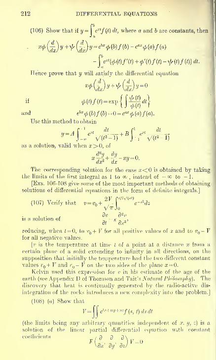
212 DIFFERENTIAL EQUATIONS
n(106) Show that if y = 1 e*'/(0 dt, where a and 6 are constants, then
J a
•
x^{^ y+^{T^y=ehx ^ {h)f{h) ~^x
^ {a)f{a)
-(W(O/'(«)+0'(O/W-^W/«}&J a
Hence prove that y will satisfy the differential equation
if ^>W/(0 = exp{J^|^}
and ebx
(p(b)f(b)=0 = etlx
(f>(a)f(a).
Use this method to obtain
^J -oo V(^-l) J-l V('
2 -l)
as a solution, valid when x>0, of
The corresponding solution for the case x<0 is obtained by taking
the limits of the first integral as 1 to oc, instead of -co to -1.
[Exs. 106-108 give some of the most important methods of obtaining
solutions of differential equations in the form of definite integrals.]
(107) Verify that v = v + ^-\ e~*dz
, ,. , dv d 2vis a solution of ~= K ~-,
ot ox1
reducing, when t = 0, to v + V for all positive values of x and to v - Vfor all negative values.
[v is the temperature at time t of a point at a distance x from a
certain plane of a solid extending to infinity in all directions, on the
supposition that initially the temperature had the two different constant
values v + V and v - V on the two sides of the plane x = 0.
Kelvin used this expression for v in his estimate of the age of the
earth (see Appendix D of Thomson and Tait's Natural Philosophy). Thediscovery that heat is continually generated by the radio-active dis-
integration of the rocks introduces a new complexity into the problem.]
(108) (a) Show that
V= [ elx+my+nzf(s, t) ds dt
(the limits being any arbitrary quantities independent of x, y. z) is a
solution of the linear partial differential equation with constant
coefficients / a a 7)\
F[ , , J V=0\dx dy dz/

MISCELLANEOUS EXAMPLES 213
if I, m, n are any constants or functions of s and t such that
F(l, m, n) = 0.
Extend the theorem to the case when there are n independentvariables x, y, z, ... , and (n - 1) parameters s, t, ... .
Obtain V=f
#lxcoat+**int+u)f(8, t) ds dt
as a solution of ^ + -~~2 = a- ' P1 - Todd.]
(P) r) F)\
«-,_-, p-j F is a homogeneous linear
partial differential equation with constant coefficients a solution is
]/dx + my + nz, t) dt,
where the limits are any arbitrary quantities independent of x, y, z, andI, m, n are any constants or functions of t such that
F(l, m, n) = 0.
Extend the theorem to the case when there are n independent
variables and (n - 2) parameters. [See H. Todd, Messenger of Mathe-
matics, 1914.]n.
Obtain 7=1 f(x cos t + y smt + iz, t) dt
d2V d*V d2V .
as a solution of = .,- + -=-=• + -=-r- =0.ox* oy£ oz l
[Whittaker's solution of Laplace's equation.]
(109) By substituting the trial solution
a, a 9
y = ao + x+
x%+ ~'
.._ .,
. dy 1in the differential equation -=- + y= -
,
0! 1! 2! 3!obtain the series y =—I- „ + + .+....
x x£ x6 xr
Prove that this series is divergent for all values of x.
Obtain the particular integral
y = e~x I — dx,
J -00 X
and by repeated integration by parts show that
C' e*7
0! 1! 2! n! , f ' (n+l)!e*e x
\ —dx = - + -9 +-= + ...+ -—i + eJ —
-is dx.
j_ M X X X? XA Xn+1 J -r. Z»+2
Hence prove that if x is negative the error obtained by taking n
terms of the series instead of the particular integral is less than the
numerical value of the (n + l)th term.
[Such a series is called asymptotic. See Bromwich's Infinite Series,
Arts. 130-139.]

214 DIFFERENTIAL EQUATIONS
(110) Show that if the sequence of functionsfn (x) be defined by
f (x)=a + b(x-c), where a, b, c are constants,
and /„(*) = JV*)^(0/«-i(0^
d2
thendx^n{x)
= ~ F{x)f»-i(x)'
00
Hence show that y =^fn {%) is a solution ofo
provided that certain operations with infinite series are legitimate (for
a proof of which see Whittaker and Watson's Modern Analysis, p. 189.
They give a proof of the existence theorem for linear differential equa-
tions of the second order by this method).
(111) Prove that the solution of the two simultaneous linear differ-
ential equations with constant coefficients
f(D)x + F(D)y=0,
<t>(D)x + \f,(D)y=0
(where D stands for d/dt), may be written
x = F(D)V,
y=-f(D)V,
where V is the complete primitive of
{f(D)yl,(D)-F(D)<t>(D)}V=0.
Hence show that if the degrees of/, F, 0, \js in D be p, q, r, s respec-
tively, the number of arbitrary constants occurring in the solution will
in general be the greater of the numbers (p + s) and (q + r), but if
(p + s) — (q + r) the number of arbitrary constants may be smaller, andmay even be zero as in the equations
(D + l)x + Dy=0,
(D + 3)x + (D + 2)y = 0.
(112) (a) Prove that if y = u(x),
y= v(x)
are any two solutions of the linear differential equation of the first order
P(x)yi +Q(x)y=0,
then (t'ux- uvj/u2 = 0,
so that v = au, where a is a constant.
(b) Prove that if y = u(x),
y= v(x),
y= w(x)
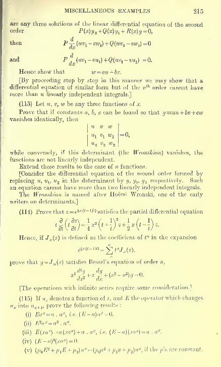
MISCELLANEOUS EXAMPLES 215
are any three solutions of the linear differential equation of the secondorder P{x)y2 + Q(x) yi + R{x)y = 0,
then P -=- («Wi - vwx ) +Q(wv1- vwj) =
and P -j-iuvi-vu^+Qi^-viij) = 0.
Hence show that w = au + bv.
[By proceeding step by step in this manner we may show that adifferential equation of similar form but of the nth order cannot havemore than n linearly independent integrals.]
(113) Let u, v, w be any three functions of x.
Prove that if constants a, b, c can be found so that y=au + bv + cwvanishes identically, then
U V wux vx wx
=0,
u 2 v2 w t
while conversely, if this determinant (the Wronskian) vanishes, the
functions are not linearly independent.
Extend these results to the case of n functions.
[Consider the differential equation of the second order formed byreplacing u, uv u 2 in the determinant by y, yv y 2 respectively. Such
an equation cannot have more than two linearly independent integrals.
The Wronskian is named after Hoene Wronski, one of the early
writers on determinants.]
(114) Prove that z = eix ( t ~ 1/t) satisfies the partial differential equation
Hence, if J n {x) is defined as the coefficient of tn in the expansion
e^-m^-^tnJn (x),
prove that y = Jn (x) satisfies Bessel's equation of order n,
[The operations with infinite series require some consideration.]
(115) If uj:denotes a function of x, and E the operator which changes
ux into ux+1 ,prove the following results :
(i) Eax = a . ax, i.e. {E-a)ax = Q.
(ii) E2ax = a2. ax .
(iii) E(xax) = a{xax)+a . ax, i.e. (E-a)(xa x)=a . a*.
(iv) (E-a)*(xax)=0.
(v) (p E2 +p 1E+p 2)ax= (pQa
2 +p1a+p2)ax
, if thep's are constant.

216 DIFFERENTIAL EQUATIONS
(vi) ux=Aax +Bbxis a solution of the linear difference equation
PoUx+z +PiUx+1 +p 2ux= 0,
i.e. {p E2 + p1E+p 2)ux =0,
if A and B are arbitrary constants and a and b the roots of the auxiliary
equation p m2 +^m^-p 2= 0. (Cf. Art. 25.)
Solve by this method (2£2 + 5E + 2) ux = 0.
(vii) ux= {A + Bx)ax is a solution of (E2 -2aE + a2)ux = 0.
Here the auxiliary equation m2 -2am + a2 = has equal roots.
(Cf. Art. 34.)
(viii) ux= rx(P cos xd +Q sin x6) is a solution of
(PoE2 +PiE + Pz) ux = ^
if P and Q are arbitrary constants, p±iq the roots of the auxiliary
equation p m? +p 1m+p 2=
and p + iq = r (cos + i sin 6). (Cf. Art. 26.)
Solve by this method (E2 -2E + i)ux = 0.
(ix) The general solution of a linear difference equation with constant
coefficients
F(E)=(p En +p 1E"-i + ...+pn_ 1E + pn)ux =f(x)
is the sum of a Particular Integral and the Complementary Function,
the latter being the solution of the equation obtained by substituting
zero for the function of x occurring on the right-hand side. (Cf.
Art. 29.)
(x) ax/F(a) is a particular integral of
F(E)ux = ax,
provided that F(a)=f=0. (Cf. Art. 35.)
Solve by this method (E2 + 8E - 9) ux = 2x .
[For further analogies between difference equations and differential
equations, see Boole's Finite Differences, Chap. XL]

^
ANSWERS TO THE EXAMPLES
CHAPTER I.
Art. 5.
(5) The tangent to a circle is perpendicular to the line joining the
point of contact to the centre.
(6) The tangent at any point is the straight line itself.
(7) The curvature is zero.
Art. 8.
Sf*2 /y3 /y>4
(1) y = a + ax +a^ +a^ + a-rj + ...=aex .
(2) y = a + bx - a —^ - 6 —}
+ a jy + . . . = a cos x + b sin x.
Miscellaneous Examples on Chapter I.
<3> 3-«*+*-*
(^>»4IW{-(in]-V{-(2)T «3-*
« Mg)T=°<g)a
. - >*-
•
(12) y = ae x + ber*. (14) 60° and -60°.

V
ii DIFFERENTIAL EQUATIONS
(15) Differentiate and put x = l, y = 2. This gives ~ and hence p.
(17) (i) z + l=0; (ii) y2 = x2 + 6x + l.
CHAPTER II.
Art. 14.
(1) 6x2 + 5xy + y2 -9x - Ay = c. (2) sina;tan?/ + sin(a; + ^) = c.
(3) sec x tan y -
e
x = c. (4) x-y + c = \og(x + y).
(5) x + yex3 = cy. (6) y = cx.
(7) e ?/(sina; + cosa;)=c. (8) x*y + icy + 4 = 0.
(9) yex -cx. (10) sin a; cos y = c.
Art. 17.
(1) (x + y)z = c{x-y). ^$2) z2 + 2?/2 (c + log y)=0.
*(3) a;?/2 = c(a;-?/)2
. (4) ca;2 = ?/ + -v/(cc
2 + ?/2).
(5) (2x-y)2 = c{x + 2y-5). (6) (z + 5?/-4)3(3a: + 2?/ + l) = c.
(7) x-y + c = log(3x-4:y + l). (8) 3z-3?/ + c = 2 log(3x + 6y-l).
Art. 21.
(1) 2y = (x + a)5 + 2c(x + a)z . (2) x# = sin x + c cos x.
(3) 2/ log x =7Jtag\)^£. (4) cc3 =
^/
3 (3sina;4-c).
!
(5) y2 (x + cex) = l. (o) x = y
3 + cy. (7) a? = e~ !'(c + tan y).
Art. 22.
(1) The parabola y2 = 4ax + c.
(2) The rectangular hyperbola xy = c2 .
(3) The lemniscate of Bernoulli r2 = a2 sm20.
(4) The catenary y = k cosh -^—
.
(5) xy — c2.. \J
(6) i/S = a;
§ + c§
. (7) yv = c&. (8) r2 = ce^.
(9) log r + 102 + JO3 - c. (10) The equiangular spirals r = ce±e tan a.
Miscellaneous Examples on Chapter II.
V(1) xy = y* + c. (2) cx* = y + ^/(y
2 -x2).
(3) sin xsiny + e 8in r = c. (4) 2x2 - 2xy + 3y + 2cx2y = 0.
(5) cxy = y + \/(y2 -x2
). (11) x3y~2 + 2x5y~'i = c.
(12) tan-1 (^)+log(«/2/)=c. (14) (x2 -l+y*)ex* = c.
(15) (i) The Reciprocal Spiral r(0- a ) = c.
(ii) The Spiral of Archimedes r= c(6-a).
(16) The parabola Sky2 = 2x. (18) x = y(c -k log y).

ANSWERS in
(19) (i) a? + (y-c)2 = l +C2, a system of coaxal circles cutting the given
system orthogonally,
(ii) r2 = ce-63
. (id) n2 = r{c + log(cosec nQ + cot n$)}.
<*» ("'gX-'D-f -»•
(21) log(2a;2 ±an/ + */2)+7^tf _!»±2y
xy/1=o. 4
CHAPTER III.
Art. 28.
(2) y =A cos 2x + B sin 2x.
(4) y = e2x(J. cos a; + B sin a;)
(6) s =A + Be- 4t.
(8) ?/ = 2e- a! -e-2a!.
(1) y^^e-^ + ^e"3 *.
(3) y = Ae~3x + Be-*x .
(5) s = e- 2t(^cos3« + 5sin30.
(7) y =Aex + Be-x + Ce~2x .
(9) ?/ =4 cos (2a; -a) + 5 cos (3a; -/3).
(10) y = A cosh (2a? - a) + £ cosh (3x - /3), or -
y - Ee2x + Fe~2x + Ge*x + He~3x .
(11) y = Aer** + Be* cob {xy/3- a).
(12) y = Ae2* + Be"2* + Ee~x cos (aj-y/3 - a) + Fex cos (xV3 - /3)
(13) 6 = a cos *vW- (14
) ^2 < 4mc -
(16) Q-Qf-nWcoBt^^-R2 \
iL2)'
Art. 29.
(1) y = ex(l+Acosx + Bsinx). (2) ?/= 3 + 4e a; + Be12 *.
(3) y = 2 sin 3a; + A cos 2a; + B sin 2a;. (4) a = 2; 6 = 1.
(5)a-6;ft--l. (6) a = /£; p = 2. (7) a = l.; 6 = 2; y-1.
(8) a = 2. (9) 4e3*. (10) 3e7 *.
(11) -f sin 5a;. (12) £ cos 5a; - £ sin 5x. (13)2.
Art. 34.
(1) y = A + Bx + (E+Fx)er*.
(2) ?/ = (A + Bx + Cx2) cos x + (E + Fx + Gx2
) sin a;.
(3) «/ = (.4 + Z?a;) e* + 2? cos a; + .F sin a;.
(4) y = A + Bx + Cex + {E + Fx)e-^..
Art. 35.
(1) y = 2eZx + e~3x (A cos 4a; + Bsin 4a;).
(2) y = e--P*(4 cos qx + B sin </x) + eax/{(a + p)
2 + q2}.
(3) y = (A+9x)e3x + Be-3x .
(4) «/ = 4+(B + |j)e a: + (C + |a;)e- a:.

IV DIFFERENTIAL EQUATIONS
(5) y - [A + ax/2p) cosh px + B sinh px.
(6) y =A+(B + Cx-2x2)e-2x.
Art. 36.
(1) y = 2sin 2a;-4cos2x + ile- a!.
(2) */ = 4 cos 4a; - 2 sin ix + Ae2x + Be3x.
(3) y = 2co&x + e-*x{Aco&Zx + BsmZx).
(4) !/ = sin 20a; + e- a!(^ cos 20a; + 5 sin 20a;).
Art. 37.
(1) y = x3 -3x2 + 6x-6 + Ae~x. (2) y = 6x2 -6x + A + Be~2r.
(3) y^Gx + e +^ +^e3^
(4) </ = a;3 + 3a;2 + ^a; + i?
, + (^ + JBa;)e3a; .
(5) y = 24x* + Ux-5 + Ae- x + Be2x .
(6) # = 8a;3 + 7a;
2 - 5ic + .4er* + Be2x + C.
Art. 38.
(1) 2/ = ^4 cosa; + (l? + 2a;)sina;. (2) y = Aex + (x + 2)e*x.
(3) y = ^4e2a: + (B + Gx - 20a;2 - 20a;3 - 15a;4 - 9a^) e"*.
(4) y = {Asinx + (B-x) cosx}e~x.
(5) y = (^ + Bx - x3) cos x + (E + Fx + 3x2) sin x.
(6) s/=^ + (£ + 3a;)e a! + Ce-K + a;
2 + £cosa; + (jF + 2a;)sina;.
(7) y ={A sin 4a; + (B- x + x2) cos 4a;}
e
3*.
Art. 39.
(1) ?/ = ^a; + J5x2 + 2x3 .
(2) y = 2 + ^lar4 cos (3 log x) + Bx~* sin (3 log x).
(3) y = 8 cos (log a;) - sin (log as) + via;"2 + Sx cos (^/3 log a; - a).
(4) i/ = 4 + log x + Ax + Bx log x + Cx (log x)2 + D'x (log a;)3
.
(5) y = (l + 2a;)2 [{log (1 +2x)}2 + ^ log (1 +2a;) + B].
(6) y =A cos {log (1 + a;)-ct} + 2 log (1+a;) sin log (1+x).
Art. 40.
(1) y^A cos (x-a) ; z—-Asin(x-a).
(2) y = Ae^ + Be3x ; z = 6Ae5x -7Be3x.
(3) y = Aex -?B cos (2x -a); z = 2Aex -B cos (2x - a).
(4) ?/ = e a; + ^ + JBe-2a;; 2 = e
x + A - Be~2x.
(5) y = A cos (x-a) + 45 cos (2a; -ft) + cos 7a;
;
z =A cos (x - a) + B cos (2a; - (3) - 2 cos 7a;.
(6) y = - S^e3* - 4 JBe4* + 2e-* + cos 2a; - sin 2a;
;
z = Ae3x + Be*x + 3e~ x + 4 cos 2a; + 5 sin 2a;.

ANSWERS
Miscellaneous Examples on Chapter III.
y=>{A + Bx + Cx2)ex + 2e?x . (2) y = {A + Bx + 6x*)e-**fi.
y = Ae~Zx + Be~2x + Cerx+Ex + 2e-2*(sin x - 2 cos a;).
y4Aex + B cos (2x - a) - 2e ie (4 sin 2x + cos 2a?).
y = (A + Bx + Gxi)e-x + (E + x + 2x2)e3x .
y=A &in(x -a) + B sinh (3x — yS) — 2 sinh 2x.
y = (A + Bx + 5x2) cosh x + (E + Fx) sinh x.
y m 3 + 4x + 2X2 + (A + Bx + 4x2) e2x - cos 2x.
?/ = (J. + Bx + 3 sin 2a; - 4x cos 2a; - 2a;2 sin 2a;) e2x .
y =A cos (x - a) + f - ^- cos 2a; - Jx cos a; + TV sin 3a;.
y =A cos (a; - a) + B cos (3a; - f3)- 3aTcos x + x cos 3a;.
y = (A + A xx + A $? + . . . + Aa^x*'1
) eax + ax/(\og a - a)a.
y =A + B\ogx + 2(\ogx)3 . (14) y =A + Bx^ + jx2.
y = Ax~3 + B cos (\/2 log x - a).
y = A + B log (x + 1) + {log (x + 1)}2 + x2 + 8x.
x=A£ l + Be~zt + E cos t + F sin t - el
;
y =Aest + 25e~3t + (32? - 42?) cos « + (3F + 42?) sin « - e(.
x = ^4e2 < + Be~ l cos(V3J - a)
;
y = Ae21 + Be~ l cos (^/3t - a + 2tt/3) ;
e = Ae21 + Be-1 cos(V& - a + 4tt/3).
x =^ + 2?H; y = Bt-x -At.
x= At cos (log £ - a) + 2ft-1 cos (log t-fi);
,y = At sin (log £ - a) - 2ft-1
sin (log £ - /S).
(i) (x-l)e2a;;
(ii) £(x2 -2a; + l) sin x + \{x2 - 1) cos x.
y = e2x + Aex.
y = (sin ax)/(p2 -a2)+A cos px + B sin yx.
?/ = .4eaa: + J8e6a: + e6x xe-6x (log x - 1) dx.
(iii) ?/ = J. cos (x - a) - x cos x + sin x log sin a;.
(i) k/(2phe);
(ii) zero.
2/= E cos nx-vF sin «x + (? cosh wx + H sinh wx.
CHAPTER IV.
Art. 42.
a* 82:
(1)dy= a
dx'
d2z d2z(2) sr-s + =-s = 0. (Laplace's equation in two dimensions.)
ox2 ay2
.,, a2* a2* 1 a2z ... a? a?(3)
ax2+
av2=
o2 a^ W»s +ap *-°"

VI DIFFERENTIAL EQUATIONS
(5) b^- + a=- = 2abz. „ .
ox dy \
^ Xdx
+ydv= nZ
' (Euler
'
s theorem on Homogeneous Functions.)
Art. 43.
(1)3*z
dx2dz
-w <2 >
d2z d2z d2z
dx2+df
+W= 0. (3)dz dz
dx dy-1
(4) z =dz dz (dz\<
Vdx + y dy
+\dx) <&
(9) 4:Z =(dz\2 /dz\2
\dx)+\dy)' (6)
dz dz
dx dy
Art. 45.
(1) y = Ae-P(*+ t). (2) z =A sin px sin pay. (3) z =A cos p(ax-y).
(4) V = Ae-Px+w sin Zy/{p2 + q2), where p and q are positive.
(5) V = C cos (pqx + p2y + q
2z).
(6) V = Ae~rt sin (mw/Q sin (mry/l), where m and n are any integersand rl2 = 7r
2(m2 + w2).
Art. 48.
(1) — (sm x + ^sin 3a; + isin 5x + ...).7T
(2) 2(sin a- a sin 2x + ^sin 3x~ ...).
2|"/7r3 6tt\ . /tt3 6tt\ . /tt
3 6tt\ . n 1
41" 2 4 6 1(4 ) - \jpZi
sln 2a; + pTTi sin 4x + gaTi sin 6» + . .
.
J.
2(5) - [|(1 + e*) sin » + f (1 -e') sin 2^4-^(1 +e") sin 3zx H-^l-e*) sin ix + ...].
/*» 32 ^> * . Mr/. . Mr Mr\ .
(6) —2i ^3sm 2" I
4 Sln T " W7r cos T/ sln nx"
(7) (a) (2), (3), and (6) ; (6) (6).
Miscellaneous Examples on Chapter IV.
... d2V 1 dV d2V a2 df 2
dV\
(7) V = V e"Jx sin (nt -gx), where g = + ^(n/2K).
(12) F = - (e- A'
( sin B + ^ye-5'*' sin 3a; + yi^e-25A7 + ...).
7T
(13) Replace x by ttz/Z, t by tt2///
2, and the factor 8/tt by 8P/tt3 .

ANSWERS vii
(14) V = Z~ - (e~iKt cos 2x + \e-™Kt cos ix + ler***1 cos 6x + ...).b
(15) V =— (e~Kt sin x + $e-°Kt sin 3x+ le-™Kt 8in 5x + ...).
[Notice that although 7 = 100 for all values of x between
and ir, V = for x = or 7r, a discontinuity.]
(16) Write 100- V instead of V in the solution of (15).
4F«(18) F =—&
{e-*W cos{ttx/21) +^r9W/«!cos (3?re/2Z) + ...}.
7T
(19) ?/ =— (sin x cos ttf - A sin 3a; cos 3?tf +^ sin 5x cos 5vt - ...).
7T
(22) gj^ = 0; y=f(x-at) + F(x + at).
CHAPTER V.
Art. 52.
(1) (y-2a?-c)(y + 3a:-c)=0. (2) (2?/-:r2 -c)(2,>/ + 3:r2 -c)=0.
(3) 49(t/-c)2 = 4x7. (4) (2?/-cc2 -c)(2x-2/2 -c)=0.
(5) (2y - x2 - c) (y - ce x) (y + x-1 - ce~ x) = 0.
(6) (y-ex -c){y + er x -c)=Q.
Art. 54.
(The complete primitives only are given here. It will be seen later
that in some cases singular solutions exist.)
(1) z = 4^ + 4^3; y — 2p2 + 3p4 + c.
(2) x = ±(p + p~1); y = }p
2 -%\ogp + c.
(3) (p-l)2x = c-p + logp;(p-l)2
y = p2 (c-2 + \ogp)+p.
(4) x = ±p2 + 3^ + 3 log (p-l)+c; y = jP + %p
2 + 3p + 3 log (p-\) + c.
(5) x = 2 tan_1p - p~x + c; y = log (p
3 + p).
(6) a5=p + ce-^; y = %p2 + c (p + l) e~i>.
$ (7)# = 2p + cp{p2 -iy h; y=:p2 -l+c(p2 -l)~h
.
'(8) z=smp + c; y—p sin j) + cos p.
(9) aj = tan^» + c; y = pta,np + \ogcos p.
(10) cc = log (p + l) -log (p-l)+log^ + c; y = p-\og (p
2 - 1).
(11) x = p/(l+P2)+tan-V, 2/= c-l/(l+ ?
;2). (12) c = l.
CHAPTER VI.
Art. 58.
(1) C.P. (y + c)2 = xz
; x = is a cusp-locus.
(2) C.P. {y + c)2 = x-2 ; S.S. a: = 2.

yiu DIFFERENTIAL EQUATIONS
(3) C.P. tf+cy + c2^; S.S. y2 = 4=x*.
(4) C.P. c*(y + cosx) -2c sin x + y -cos x = 0; S.S. ?/2 = l.
(5) C.P. (2x* + 3xy + c)2 -4(x* + y)* = 0; x2 + y = is a cusp-locus.
(6) C.P. c2 - 12cxy + 8cf - \2x2y2 + 1 Qx3 - ; y
2 - x = is a cusp-locus.
(7) C.P. c2 + 6cx«/ - 2c?/3 - a?(3?/2 - a;)
2 = ; «/2 + x = is a cusp-locus.
Art. 65.
(1) C.P. (y + c)2 = x(x-l){x-2); S.S. x(x-l)(x-2)=0 ; z = l-l/y3
is a tac-locus and x = l + l/\/3 a tac-locus of imaginary points
of contact.
(2) C.P. (y + c)2 = x(x-l)2
; S.S. z = 0; a; = 1/3 is a tac-locus; x = l
is a node-locus.
(3) C.P. y2 -2cx + c2 = 0; S.S. ?/
2 = a:2
.
(4) C.P. x2 + c(x-3y)+c2 = 0; S.S. (3y + a)(y -x)=0.
(5) C.P. y-cxa -c2 = 0; S.S. z4 + 4?/ = 0; a; = is a tac-locus.
(6) C.P. y = c(x-c)2; ?/ = is a S.S. and also a particular integral;
27*/-4a;3 = 0isaS.S.
(7) Diff . Eq. p2y2 cos2a - 2pxy sin2a + y
2 -x2 sin2a = ;
S.S. y2 cos2a = x2 sin2a ; y = is a tac-locus.
(8) Diff. Eq. (a;2 -l)j92 -2a^-a;2 = 0; S.S. x2 + */
2 = l;
x = is a tac-locus.
(9) Diff. Eq. (2x2 + l)p2 + (x2 + 2xy + y2 + 2)p + 2y2 + l=0;
S.S. x2 + 6xy + y2 = 4 ; # = ?/ is a tac-locus.
(10) Diff. Eq. p2 {l-x2)-(\-y2)=0; S.S. x= ±1 and y= ±1.
oMj fab:
Art. 67.
S.S. z2 + 4?/ = 0.
(2n^ W^3; S.S. 27/ + 4a:
3 = 0.
(3) C.P. y — cx + cos c ; S.S. (y - x sin_1
a;)2 = 1 - x2 .
(4) C.P. y = cx + ^/(a2c2 + b2 ) ; S.S. x2\a2 + xj2\h2 = \.
(5) C.P. y = cx-ec; S.S. ?/ = a;(log a;-l).
(6) C.P. ?/ = ca:-sin-1c; S.S. y= V(x2 -1) -sin-V(l ~V^)-(7) \{y — px)2 — —pk2
; 2xy = k2, a rectangular hyperbola with.
axes as asymptotes.
(8) (x - y)2 -2k(x + y)+ k2 — 0, a parabola touching the axes.
(9) The four-cusped hypocycloid a;3 + y* —k*.
Miscellaneous Examples on Chapter VI.
(1) No S.S. ; a; = is a tac-locus.
(5) 2y=±3x represent envelopes, y — is both an envelope and a
cusp-locus.

ANSWERS IX
(6) C.V.xy = yc + c*.
(7) C.P. x = yc + xyc>; S.8. y=0, y + 4x*=0. (Putt/ = 1/F; 3 = 1/*.)
(8) (i) Putting p + x=W we get
2x = 3 (*3 - I
2) ; 40y = 9 (5«
6 + 2«5 - 5f4 ) + c.
(ii) C.P. «/2 + 4^ = 1 +2cx; S.S. a£-4y* + 4=0; ?/ = is a tac-locus.
(11) C.P. r = a{l +cos (6 -a)}, a family of equal cardioids inscribed in
the circle r = 2a, which is the S.S. The point r = is a cusp-
locus.
CHAPTER VII.
Art. 70.
(1) y=logsec x + ax + b. (2) x = a + y + b\og (y-b).
(3) ay = cos (ax + b). (4) x = log {sec (ay + b) + tan (ay + b)} + c.
(5) y = x3 + axlog x + bx + c.
(6) y= -ex + ae2x + bxn-2 + cxn
~z + ... +hx + k.
(7) The circle (x - a)2 + (y - b)2 = k2 . The differential equation ex-
presses that the radius of curvature is always equal to k.
(9) \/(l + 2/i2)= ky.} ; the catenary y-b = k cosh {(#
-
a)/k}.
Art. 73.
(1) y = x(a\ogx + b). (2) i/ = axcos (2 log x) +&csin (2 log a).
(3) y = x(a\ogx + b)2 . (4) y = x2 (a log x + b)2 .
Art. 74.
(1) y=±cothX-~^. (2) y- -log(l-x). (3) y = sm-1
x.
(5) (i) The conic m = yu//t2 + (1/c - /x//t
2) cos B \
(ii) cm = cos 0\;(l - nlh2) or cosh 6^(m/h2 -l), according as /u>/*8 .
Art. 75.
(1) y = a(x2 + l)+be~ x. (2) y = a(x-l)+kr*.
(3) y = a(x-l)+be~x + x2 . (4) y = l +e~^. (5) y-e8 ".
Art. 77.
(2) y = xz + ax-l\x. (3) y = (<c2 + ace) e* + to.
(4) y = e2x + (ax* + b)ex. (5) y = ax3 + tar3 .
(6) «/ = ax2 + b sin as.
Art. 80.
(1) y = (a - x) cos x + (6 + log sin x) sin x.
(2) y= ja-log tan ( j +ajjJ-
cos 2x + &sin 2x.

X DIFFERENTIAL EQUATIONS
(3) y = {a-er* + \og{l+er")}ex + {b-log{l+ex)}erx .
(4) y = ax + bx~1 + (l-x-1)ex . (5) y = aex + (b-x)e?x + ce?x.
Miscellaneous Examples on Chapter VII.
(1) y = aee'h -b. (2) y = a + \og{x2 + b).
o^n+i xn xn—*
(3) v= ; rTT + 2a—,+ a2 -. —, + bxn
~2 + cxn~z +
.
. . + hx + k.v * (n + l)\ n\ {n-\)\
(4) y = - 32~n cos {3x - \tt (
n - 2)} + a cos a; + 6 sin x + ex"-3 + . . . + foe + k.
(5) t/ = ax + b log x. (6) y = aex + b(x2 -l)e*x.
(7) w = a cos nx + b sin nx + ~ sin was—^ cos wx log sec nx.v
'* n n2
(8) ?/(2a; + 3) = aloga; + 6 + ea:
.
(9) (i) y = \/(ax + b);
(ii) t/ = ^/(alog x + b).
(10) ?/ = (a cos x + b sin x + sin 2x) ex2
.
(12) ?/ = x22. (14) Z=-£.
(17) (i) y = ae*2 + fo-**
2 - sin x2 . (Put 2 = x2 .)
(ii) ?/(l+x2)=a(l-x2) + &x. (Putx = tanz.)
(18) j^-2y = 2{l-z2) ; ?/ = sin2 x + 4 cos (V2 sin x + a).
(19) y = acos{2(l+B)e-*} + 6sin{2(l+x)e^ x} + (i+*)e~"
CHAPTEK VIII.
Art. 83.
(1) y = 2 + x + x2 - ^x4 - fvx5; exact solution y = 2 + x + x2
.
(2) £/= 2x - 2 log x - ^ (log x) 3
; exact value y = x H4 -
.
(3) ?/ = 2+x2 + x3 + t3tfx5 + tV:k6
;
2 = 3x2 + fx4 + fx
5 + ^x7 + /^x8.
, (4) y = 5 + x + -^x4 + -^x6 + ^3x7 + TVx
9;
2 = 1 + ?, X3 + x5 + I X6 + ^X8 + 5VTX9 + 2 * i x
11.
(5) 2/ has the same value as in Ex. 4.
Art. 87.
(1) 2-19. (2) 2-192. (3) (a) 4-12; (6) 4-118.
(4) Errors 0-0018 ;0-00017 ; 0-000013 ;
Upper limits 0-0172 ; 0-00286 ; 0-000420.
Art. 89.
1-1678487; 1-16780250; 1-1678449.

ANSWERS xi
CHAPTER IX.
Art. 95.
(1) „w|i-* +_-...|»cobV3; v = a;i|l-|j+^-...|=8inV*.
„L 8 8.11 „ 8.11.14 , I
(4) ^ XH 1 "4TO x2 +4.8(l +l)(2 + n)
^
1 6 \4.8.12(l+w)(2 + n)(3 + w)
a; +"'J'
To get v from u change n into -n. If u is multiplied by
the constant r-^, — , the product is called Bessel's functionAni (n + 1)
of order n and is denoted by Jn (x).
Art. 96.
(1) and (4), all values of x. (2) and (3), |x|< 1.
Art. 97.
f\ 2. 2.5, 2.5.10 . 1
v = u log a; + { - 2x - x2 - ^4-x3 . . .}.
(2) u = |l -
-
2x2
+ ^-p^4 _22
. 42 . 62a;6 + ""
J
'
t> = Mlogg+|^g2 -^-^i(l+^)g* +
22 ^^ 62(l+| + ^)g
B-...j.
m is called Bessel's function of order zero and is denoted byJ {x).
(3) u={l-2x + ^x*-^x* + ...y,
v = u\ogx+^2(2-i)x-~(2 + l-l)x^ + ^(2 + h + l-l)x3 -...y
if. 1.3 . 1.3.5.7 . 1.3.5.7.9.11fi
1
(4) MBa?»|l+— a*+^ gg
s*+ ^ 82—
2l x6 + ...|;
M *}
v = w log x + 2ar 1 t2 (1 + i - 1) x2
P.D.E. p 2

xii DIFFERENTIAL EQUATIONS
Art. 98.
i
.r8
23 . 42 . 6 .
8
(1) u-x 2{- 22. 4*4 +
237T76a;6 ~23 .42 .6.
ro*10-] ;
v = u\ogx +x-^l+^x2 +¥-^-^-^ 2̂x9
318 |+
22A2 .62 .82X "')'
(2) u = x + 2x2 + 3x* + ...=x(l-x)-2;
v = u log x + 1 + x + x2 + . . . = u log x + (1 - a;)-1
.
(3) w = {1.2a;2 + 2.3x3 + 3.4x4 + ...};
v = ulogx +{-l+x + 3x2 + 5xs + lxi + ...}.
(4) M = {2a5 + 2a;2 -a;3 -a^ + |«5...};
v = u log x + {1 - x - 5x2 - x3 + V"*4
. . .}.
Art. 99.
(1)2/ = a {l - z2 - ix4 - is". . .} + ajx = a |l - |a log^J + axx.
(2) y^ji-^^^-^;; 1)^^ -..,} .
f (n-l)(n. + 2) (n-l)(n-3)(n + 2)(n + 4 ) . \+ ai
l 3!* +_ ~5T~ "7*
[For solutions in powers of 1/x see No. 7 of the Miscellaneous
Examples at the end of Chapter IX.]
(3) y^{l-0^ + 17^ a?8 -
3.4.7.8.11.128l, + "j
+ a^-0^5 +4T5V9 x9 -4.5.8.9.12.13
xl3 + --} <
(4) y = a {l - ^a2 - T\x3 + &x*...} + a x{x - \x* - ^x* + &*. . .}.
Art. 100.
(1) z^ + z^+{\-n2z2)y = 0. (2) y = ax2 (l+2x).
(3) y = x2(1 + 2b) {a + 6
jor2 (1 + 2x)~2 e* dx}.
(5) 2e-and[2e-log 2+22 {l-|]
(l+i) 2 +|I
(l+^ +^2-...}],
where z = \jx.

ANSWERS xiii
Miscellaneous Examples on Chapter IX.
(1) u = x~l |l +- x +^x2 +~x3 +...J;
(13 9 _ 27 . )V=
\l!+
4!a; + 7!^ + lT!
K+ -} ;
i/l 3 9 _ 27 . I
-^\2l+6lX+8!^ + lT!^+-T
(2) M,|l+J- a;+ -l^ a;2 +i2 ^ 32
a*+„.}; '
t, = *dogz +2|-pS-pr-^(l+-) a;2
1 2 .22 .32 \ 2 3/ '"/'
w = u (log a;)2 + 2 (v - u log a;) log x
CHAPTER XI.
Art. 113.
(1) x/a = y/b = z', straight lines through the origin.
(2) lx + my + nz = a ; x2 + y2 + z2 = b; circles.
(3) y = az; x2 + y2 + z2 = bz; circles.
(4) x2 -
y
2 — a ; x2 -2;2 = 6; the intersections of two families of rect-
angular hyperbolic cylinders.
(5) x-y = a (z-x);(x-y)2 (x + y + z) = b.
(6) x2 + y2 + z2 = a
; y2 - 2yz -z2 = b; the intersections of a family of
spheres with a family of rectangular hyperbolic cylinders.
(7) y/(m* + n2)
. (8) The hyperboloid y2 + z
2 - 2x2 = 1
.
(9) (x2 + y2){k tsm-hj/x)2 = z2r
2. (10) l/x = l/y + 1/2 = \(z + 2.
Art. 114.
(1) y-3x = a; 5z + t&n(y-3x)=be^x.
(2) y + x = a; log {z2 + (y + x)2} - 2x = b.
(3) xy = a; (z2 + xij)
2 -xi = b. (4) y = ax\ \og(z-2x/y)-x= b.
Art. 116.
(1) x2 + y2 + z
2 = c2 ; spheres with the origin as centre.
(2) x2 + y2 + z2 = ex ; spheres with centres on the axis of x.
(3) xyz — <?.
XIV DIFFERENTIAL EQUATIONS
(4) yz+zx + xy = c? ; similar conicoids with the origin as centre.
(5) x-cy=y log z.
(6) x2 + 2yz + 2z2 = c2 ; similar conicoids with the origin as centre.
Art. 117.
(1) y — cx log z. (2) x2y = cz&. (3) (x + y + z2)ex2 = c.
(4) y{x + z) = c(y + z). (5) {y + z)/x + (x + z)ly = c.
(6) w/-mz = c(wa?-fe). The common line is x\l = y\m=z\,n,.
Art. 120.
(3) z = ce2*. (4) z2z + 4=0.
Miscellaneous Examples on Chapter XI.
(1) y = ax; z2 -xy = b. (2) x^y%z — a\ xz + yz = bx2y
2.
(3) y + z = aex; y
2 -z2 = b. (4) ?/ = sina; + cz/(l + z2 ).
(5) x2 + a:?/2 + x2z = £ + c. (6) f(y) = ky; xk = cyz
.
(8) <fo/a; = %/2?/ = dz/3z. (9) y + z = 3e*-3 ; y2 - z2 = 3.
(10) (i) x2 + y2 + z2 = c(x + y + z)
;(ii) x2 - xy + y
2 = cz;
(iii) y2 -yz-xz = cz2 .
(14) xt/ = cez sin w.
CHAPTEE XII.
Art. 123.
(1) <p(x/z! yfz)=0. (2) (j>(lx + m,y + nz,x2 + y
2 + z2)=0.
(3) 0{*//z, (x2 + y2 + z2)jz} = 0. (4)0 (x2 - y
2, x2 - z2 ) = Q.
(5) <p{(x -y)2 (x + y + z),(x- y)l(z - x)} = 0.
(6) (p{x2 + y2 + z2
, y2 - 2yz - z2} = 0.
(7) <f>[y-3x, e~5a:{5z-tan(«/-3a;)}]=0.
(8) </>{y + x, log (z2 + y
2 + 2yx + x2 )- 2x) = 0.
(9) y2 = ixz. (10) a(x2 -y2)+b(x2 -z2)+c = 0.
(12) (j>(x2 + y
2, z) =0 ; surfaces of revolution about the axis of z.
Art. 126.
(1) (fi{z + Xx,X1JfX 2,X-i + X3)=0.
(2) 0(z, xfrf1, xfxf1
, a; 1%r1)=°-
(3) (p(z-x 1x 2 , a^ + Xa + Zg, x2x3)=0.
(4) 0(2z + a; 12
, x x2 -x 2
2, x x
2 -x32)=0.
(5) (p(4\/z ~ xz2
> 2x3 -x22
, 2x 2 -a; 1
2)=0; special integral z = 0.
(6) <p{z-3xv z-3x 2 , z + 6\/(z-x 1-x2 -x3)}=0; special integral
Z == X-\~tX 2 ~tX3 .

ANSWERS XV
Art. 129.
(1) z = (2b2 + l)x + by + c. (2) z = a;cosa + y8in a + c.
(3) z = ax + y\oga + c. (4) z = asx + a~2y + c.
(5) 2 = 2x sec a + 2y tan a + c. (6) z = a;(l + a) + ?/(l + l/a) + c.
Art. 130.
(1) az = (a + ay + bf. (2) z=± cosh {(a; + ay + 6)^(1 + «2)}-
(3) z2 -a2 = {x + ay + b)2 , or 2 = 6. (4) z2 (l+a3)=S{x + ay + bf.
(5) (2 + a)e a!+a2/ = 6. (6) 2 = 6eax+aX
Art. 131.
(1) 3z = 2(x + a)* + 3ay + 3b. (2) 2az = a2x2 + y2 + 2ab.
(3) az = ax2 + a2x + eav + ab. (4) (2z-ay2 -2b)2 = l6ax.
(5) 2 = a(ex + e2/) + 6. (6) az = a2x + a sin x + sin */ + a6.
Art. 133.
(1) 2 = - 2 - log xy. (2) 3z = xy-x2 - y2
. (3) 823 = - 27x2y2
.
{±)zx=-y. (5)2 = 0. (6) 22 = 1. (7)2 = 0.
Art. 136.
(1) 4«= -y\
(4) A particular case of the general integral, representing the surface
generated by characteristics passing through the point (0, -1,0).
Miscellaneous Examples on Chapter XII.
(1
)
2 = ax + by - a2b ; singular integral z2 = x2
y.
(2) zx = ax + by- a2b ; singular integral z2 = y.
(3) <j>{xy,(*2 + xy)2 -x*}=0.
(4) 2 = 3z3 - 3ax2 + a2x + 2?/4 - lay3 + 3ahj2 - a3y + b.
(5) 2 = ax x + b log x 2 + (a2 + 26) x3_1 + c.
(6) z^^^ + x^x^x^-x^}.
(7) 3a(x + at/ + 6) = (l +a3)log2, or 2 = 6. 2=0 is included in z = 6, but
it is also a singular integral.
(8) z(l+a2 + b2) = (x 1 + ax2 + bx3 + c)2
.
(9) <p(z-e4a;i, 2-e4^,2-e4^)=0. (10) z = ax- (2 + 3« + hr)y + b.
(11) 22 = az2 -(2 + 3a + ia2)2/
2 + 6. (12) 22 = (1 + a 2)x2 + aif + b.
(13) z = a tan (£ + a?/ + 6), or 2 = 6. 2 = is a singular integral, but it is
also included in z = 6.
(14) 22 = ax2 + by2 - 3a3 + 62 . Singular integral z2 = ± 2x3/9 - i/fi.
(15) z=x + y-l±2y/{{x-l){y-l)}. (1(3) z2 -xy=c.

XVI DIFFERENTIAL EQUATIONS
(17) <j>{z/x, z/y)=0 ; cones with the origin as vertex.
(18) x2 + y2 + z2 = 2xc6sa + 2yB,ma + c; spheres with centres on the
given circle.
(19) xyz = c. (This is the singular integral. The complete integral
gives the tangent planes.)
(20) The differential equation (z - px - qy) (1 - 1/p - 1/q) = has no
singular integral, and the complete integral represents planes.
CHAPTER XIII.
Art. 139.
(1) y2{{x-a)2 + y
2 + 2z} = b. (2) z2 - 2ax + a2y2 + b.
(3) z = ax + bey(y + a)~a . (4) z2 = 2(a2 + l)x2 + 2ay + b.
(5) z = ax + 3a2y + b. (6) (z2 + a2
)z = 9(x + ay + b)2.
(7) z = x3 + ax + %(y + afi2 + b. (8) z = ax + by + a2 + b2 .
Art. 141.
(l)z = a1x
1 + a 2x 2 + (1 - a>\ - «22)xz + az .
(2) z = a1x1 + a 2x 2± sin
-1(c^ag,^) + az .
(3) z = axlog xx + a 2 log x 2± xz-\/{a x + a 2) + az .
(4) 2z = a xxx2 + a 2x 2
2 + azxz2 - 2 {axa 2az)
llz log a:4 + a4 .
(5) 2{axa 2az)
x<z log z =a^2 + a 2x22 + azx z
2 + 1.
(6) ia xz = 4ax2 log xz
4- 2a 1a 2 (x1 -
#
2)- (xx + x2)
2 + ^a xaz.
(7) (1 + «!a 2) log z = (a x + a 2)(x x + a xx 2 + a 2xz + az).
(8) z = -(a x + a 2)x x + (2a x -a 2)x2 + ( -ax + 2a 2)xz
- ^{xx2 + x 2
2 + x32) ± §{xx + x2 + xz
- 2a x2 + 2a
xa2- 2a 2
2}3/2 + a3.
Art. 142.
(1) z = =h (xx + x 2)
2 + log xz + a. (2) No common integral.
(3) z = xx2 + x 2
2 + xz2 + a, or z = x x
2 + 2x 2x z + a.
(4) z = a (xx + 2x 2) + b log xz + 2ab log x 4 + c.
(5) z = a(3xx + x 23 -xz
3) + b. (6) No common integral.
(7) z = a(x1-cc 4) + fe(a; 2
-a;3) + cJor z = a(x1 -2x 2 ) + b(2xz -x4) + c.
(8) Z = 0(3.2! + z 23 -z3
3).
(9) z = (f>{x x -x /x, x 2 -x3 ), or z = 0(£ 1
-2#2 , 2x3 -x 4).
Miscellaneous Examples on Chapter XIII.
(1) z2 = axlog x
x-
a
xa 2 log £ 2 + a 2 log£3 + a3 .
(2) No common integral.
(3) z = axlog X! + a 2x 2 + (a
x + a2 )
x
z± \/{a i
(
ai + %az)x
i
3l + a 3-

ANSWERS Xvij
(4) = axlog xy + a&2 + (a
2 + a2) x3± y/{a
x (a x + 2a2 ) z
3} + 1
.
(5) 2logz = c±(x* + x* + x3z). (6) z3 =x* + x.* + x3
3 + c.
(7) 42 + aj12 + x2
2 + x32 = 0. (10) z = <p(Xlx 2 , x2 + x3 + xA , x Axb).
(11) (iii) 3z = x13 -3x1x2 +c.
CHAPTER XIV.
Art. 144.
z = x* + xf(y) + F(y). (2) z - log x log y +f(x) + F(y). ^
z=-^sinxy + yf(x) + F(x). (4) z -xy +/(y) log x + F(y).
z = sin(x + y) + -f(x) + F(y). (6) z= -xy+f(x) + e*yF(x).
z = (x2 + y2)
2 -l. ' (8) z = ^2 + 2x?/ + 2</ + ua;2 + &;r + c.
2 = (x2 + i/2)2
. (10) 2 =^+ |/(l-^)
Art. 145.
«- JP1(y+«) + JF,
2 (y + 2a;) + f8 (y + 3a;).
«=/(y-2z) + JF(2y-a;). (3) z=f(y + x) + F(y-x).
The conicoid 4a;2 - 8xy + y
2 + 8x-4:y + z=0.
Art. 146.
z =f(2y - 3a?) + xF(2y - 3x). (2) 2 =f{5y + ix) + xF(5y + ix).
z=f(y + 2x)+xF(y + 2x) + <j>(y). (4) z(2x + y)=3x.
Art. 147.
z = x4 + 2a% +/(?/ + a;) + «/(y + x).
z = 2{f-x3) +f{y + 2x) + F {2y + x). (3) V = - 27ra:
2^2
.
Art. 148.
z = ex+2!>+f(y + x)+xF(y + x).
z = x2 (3a; + y) +f(y + 3x) + xF(y + 3x).
z = - x2 cos {2x + y) +f{y + 2x) + xF(y + 2x) + <p ( y).
z = xex-y+f{y -x) + F(2y + 3x).
V = (x + yf +f(y + ix) + F(y - ix).
z = 2xl log(cc + 2y) + f(2y + x) + xF(2y + x)
Art. 149.
z = x sin y+f(y-x) + xF(y -x).
z = x* + 2x*y +f{y + 5x) + F(y - 3.x).
z = sin x - y cos x + f(y - 3x) + F(y + 2x).
z = sin xy+f(y + 2x) + F(y - x).

xviii DIFFERENTIAL EQUATIONS
(5) z = %ta,nxta,ny+f(y + x) + F(y-x).
(6) y = x log t + 1 log x +f(t + 2x) + F(t- 2x).
Art. 150.
(1) z=f{x) + F(y)+e?x<t>(y
+ 2x).
(2) z = er*{f(y -x) + xF(y- x)}. (3) 7 - 2Aehlx+M).
(4) z=f(y + x) + e-*F{y-x). (5) z = ^Aeh{x+hv) +yZB^x+7k>>\
(6) 3 = 2^en(a:C03a-H' 8in 'l». (7) z = ex{f(y + 2x) + IlAe!civ+ikx)}
(8) « = l+e- a!{(2/-a;)2 -l}.
Art. 151.
(1) z = \e2x~v + exf(y + x) + e2xF(y + x).
(2) z = l+x-y-xy + exf{y) + e-vF(x).
(3) z = sV( sin (x - 3y) + 9 cos (x - 3y) }% ZAe^+^l(4) z = x+f(y)+e-xF(y + x). (5) 2/
= |xe x+2; + 2^ej:seCa+rtana.
(6) z = e2x{x2 tan (t/ + 3z) +»/(«/ + 3x) + F(y + 3x)}.
Art. 152.
(1) y2r-2ys + t=p + 6y. (2) pt-qs=pq3
.
(3) r + 3s + * + (rt-s2) = l.
(4) pq(r-t)-(p2 - q2) s + (py - qx) (rt - s2 ) = 0.
(5) 2^7, + gtf-2^(rt-s2
) = l. (6) qr + (zq-p)s-zpt = 0.
Art. 154.
(1) z =f{y + sin a:) + F(y - sin x). (2) z =/(x + ?/) + ^(xy).
(3) y-\p-{x + y + z) = <f>(x), or z=f(x) + F(x + y + z).
(4) 2 =/(£ + tan !/) + F(x - tan */). (5) z =f(x2 + y2) + F{y/x) + xy.
(6) y=f{x + y + z)+xF{x + y+z). (7) 3z =4^
-
x2xf - 6 log y - 3.
Art. 157.
(1) p + a;-2t,=/(g>-2a; + 3y) ; A = -£.
(2) p-x=f(q-y); A = a>. (3) p-ex=f(q-2y) ; A = a>.
(4) p-y=f{q + x); p + y = F(q-x); \=±1.(5) p-y^f{q~2x) ; p-2y = F(q-x) ; A = -1 or -£.
(6) px-y=f{qy-x); \=-xox -y.
(7) z^ - z =/(z£ - 1/) ; A = z/^2 or z/y2 .
Art. 158.
(1) z = az + by - \x2 + 2xy - fy2 + c
;
z = |a;2
( 1 + 3m2) + (2 + 3m) xy + nx + <j>(y + mx)
= 2xy - \ (x2 + 3y
2) + nx + \js(y + mx).

ANSWERS XIX
(2) « = f(a* + y*)+oa; + &y + c; z^^ + y^ + nx + y^iy + mx).
(3) z = ex + y2 + ax + by + c; z = ex + y
2 + nx + yf,(y + mx).
(4) & = i(a-/3); 2/ =HV/(^)-0'(«)}; z = ™J + \{<t>{a)-y},(p)} + Py.(5) a: =£- a ; y = <t>'{a)-\[r'(l3); z = xy-<f>(a)+yj,{P)+Py.(6) z + y/m + mx-n\ogx = <p(xmy) ; the other method fails.
(7) z2 = a? + y2 + 2aa; + 2oy + c; z2 = x2 + y
2 + 2nx + \J,(y + mx).
(8) 2z = y2 -a;2 .
Miscellaneous Examples on Chapter XIV.
(1) z = x2y2 + xf(y) + F(y). (2) z= e*+v+f(x) + F(y).
(3) yz == y log y -/(a) + yF{x).
(4) z=/(cc + ?/)+a;i,
(a; + ?/)-sin(2a; + 3?/).
(5) 2=/(y + loga;)+*JP(y + loga;). (6) z = x + y+f{xy) + F(x2y).
(7) 3 = log(* + y) ./(a;2 -
1/2) + *V - if).
(8) 42 = 6a;y - 3a;2 - 5y2 + lax + 46?/ + c;
4z = 6a;?/ - 3a;2 - 5y2 + 2nx + 2\js (y + mx).
. (9) 3z = 3c±2{x + a) 3l'2±2(y + b)3'2
.
(10) mz + sin y +m2 sin x - mnx = m<f>(y + mx).
(11) 2a; = «-/3; fy= ^'(/3) - 0'(«) J
22 = 3a;2 - 6^ - 7y2 + </>(«)- -f (/3) + 2fty.
(12) z = x3 + ?/3 + (a; + ?/ + l)2 . (13) z = x2 -xy + f.
(20) px + qy=f(p2 + q
2); py -qx= F(q/p).
Miscellaneous Examples on the Whole Book.
?(1) {x2 -y2
)
2 = cxy. (2) ?/ = a;2 + ce- r2
.
(3) 2 sec a; sec ?/ = a; + sin a: cos a; + c. (4) (a;?/ + c)2 = 4(a;2 + ?/)(?/
2 -ca;).
(5) 1 +a;?/ = y/(c + sin-1x)v/(l -a;2 ). (6) y = (^ - ]x) cos 2x + JBsin 2a;.
a;2
6a; 28 1
(7 ) !/ =^-^ +]2? +^^ a: (sin2a;-cos2a;) + Je- a: + 5e a: cos(2a; + u).
(8) y =A + Bx + Cx log x + log x + |a;(log x) 2 + la;2
.
(9) y + sec x = c tan a;.
(10) a; = Ae lt + Be"2' - f (cos « - sin <) ; y = ,4e2( - 3/fr- 2 < - « cos t.
(11) a;2 /3 = (y-l) 2/3 + c. (12) y = acosvc(b-x).
(13) y = L4 + Bx +X
Jsin 2x + ( J0 + Fx -
Jcos 2a;.
(14) 2xy = 3x2 + c. (15) z + xy = c(x + y -xy).
(16-) a;3 + y
3 + 23 = ca;v/z. (17) 2 =/(.n/) - Jx2 - -J y
2.
(18) (x - y)^-^^) =/{(» - 3y + z)/(x - yf).
(19) (2 + a;)2 = (2 + 2y)/0//x-).
(20) z = ax + by + a2 + b2 ; singular integral iz + x2 + ij- = 0.
(21) z = e*f(x-y) + F(y).

XX DIFFERENTIAL EQUATIONS
(22) z = aa*2 +% + 4a2 ; singular integral 1 62 + cc4 =0.
(23) z=f(x + y) + F(x-y) + b(x* + f).
(24) z = xf(y) + yF(x). (25) cz = (x + a)(y + b).
(26) z = lxy+f(y/x) + xF(yfx). (27) z=f{z + x) + F(z + y).
(28) y(x + c) = c2x; singular solutions y = and «/ + 4a;2 = 0.
(29) atf = {x + bf. (30) 2/=^cos(|^) + 5sin(^).
(31) r5 + «/2 + z2 = 2(a;cosa + ?/sina + c). (32) y = ex -\
e
ix + \^x.
(33) a; = e~Kt (a cos X£ 4- b sin XZ) + C cos (pt - a),
where C = .4/^/{(/c2 + X2 - flf + ±K2p
2}, tana - 2KpJ(K
2 + X2 - 2>2),
and a and 6 are arbitrary constants.
(34) y =A cos (sin x) + B sin (sin x).
(35) (i) i^ = ^log(r + 2) + 5;
(ii)<f>-A
[e-^4a
'2 d£+ 5 ; |^ =~ e^l***.
(36) F =A{\ + f (3z2 - r2) + ^V (35z4 - 30z2r2 +3r%where r2 = x2 + y
2 + z2 .
l+- + 7T-I + £7-*+'» COsh<a 4! a4 5! a5 /
«(£X3 X6 X \ . ,
2 + K7—3 + ^7—6 + srj—7 + -- Jsinn*.12 31a*1 6 ! ab 7 ! a7 /
(41) y-x = c(xy -l)e~x.
(42) ?/ = (l+a;) a-6 (l-cc)a+V + ^f(l+^)_0+6-1 (l-^)"a"6-1 ^}-
If 2a is an integer, the integral can be evaluated byputting z = ( 1 + x)/( 1 - x)
.
(43) (i) y = (l-x2){A + B\ogx); (ii) y = {l -x2)(x + A + Biogx).
(44) (1 - x2) y = (a + b e-*
2oa;) e^
x'
2- [Put log y = (w -
1
P) dx. u = x is
a solution of the differential equation in u.]
<M fM-l (2»-2)x2 (2H -2)(2n-4)(2n-6) x4 .
l«);/w (2n-l)2! (2«-l)(2n-2)(2n-3) 4! *" •
(2w-2)(2w-4) a3
^ (a;, ~" (2n-l)(2n-2)3!+ ""
(46) */ = ,4a-5 + J5r} + #(a;2 + l), replacing C/6 by £.
m--^**^©1
c{c + 2(6 + l)}{c + 4(6 + 3)} /x\ 6
+6!
' W +
5
+ ..,
Va/ 3! Va/ 5! Va/
both converge within the circle \x\ < \a\.

ANSWERS xx i
(50) q ji ^- i must be a function of x alone ; x*y - ax2
y2 = c.
(51) x* + y2 + 2bxy = 2ax.
(52) uvew= a IvV dx + 6, where t; = Q/P and w = It; dx.
(53) Pwcot(nx + a)+Q = n2.
(54) y(l-x)=A(3 - 2x) e2x +B(l-2x) e~2x.
(56) x3 + yz = c(y + z).
(57) t/= ^e-2a5 + e a;(5cosa;V3 + Csina;V3 )
+ t x2 +2riTir e_2a;{157x(6 cos a; + 11 sin a;)
+ 3 (783 cos a; -56 sin x)}.
(58) ^ = (3 + 4a;2){^ + £f(3 + 4a;
2)-2e-^2
^}.
(59) z*(x + y)*{x2 + y2 + z2)=c{x2 + y
2 -z2). (60) xz = c(y + z).
(62) (1) Put «= rr-5~; (") y~K=-r -•* ua 2 (x) dx K
'v
2 l-ctanz[See Ex. 41 for method.]
(65) If a particle P moves so that its velocity is proportional to the
radius vector OP and is perpendicular to OP and also to a
fixed line OK, then it will describe with constant speed a
circle of which OK is the axis.
(67) r2sin 2(0 + a) = l ; singular solution r*=*=l.
(68) y2 - x2 = ex + 2a2 + a\/(4a2 - c2
) ; singular solution y2 - x2 = ± 2ay.
(70) ia(y - c) = (x - c)2
; singular solution «/ = x -a.
(71) x + a = c cos (j) + c log taji |0. (72) a cos + b cos 0' = k.
(74) 2c?/ = (a; + c)2
; singular solution y(y -2x)=0.
(75) a;+j9«/ + ajj2 = 0; (2/ + a^)v/
(p2 + l) = c + a sinh-1^,
xV(P2 + l)+p(c + a sinh-1^) = 0.
There is no singular solution. The ^-discriminant y2 = iax
represents the cusp-locus of the involutes.
(77) y = ax,z = b + V(x2 + y2); * = V(*
2 + //
2) +/(.<//•')•
The subsidiary integrals represent a family of planes through
the axis of z and a family of paraboloids of revolution with
the axis of z as axis ; the general integral represents a family
of surfaces each of which contains an infinite number of the
parabolas in which the planes and paraboloids intersect.
(78) x2 + y2 + z2 =f{x2 + y
2 + (x + y)2} ; a;
2 + if + z2 = c2 ; z2 = xy.
(79) (2x-y)'7 = c5z{x + 2y).
(80) (ax - by)j(z + c) =f{(ax + by)j(z - c)}.

xxii DIFFERENTIAL EQUATIONS
(81) (i) I=EIR + Ae- Rt'L;
(ii) A = I -E/R; (iii) I=EjR.
(82) I = a cos {pt - e) + Ae -Rl'L
, where a = E/^R2 + L2p2), tan e- Lp/R,
and A is arbitrary.
(83) Q = a sin (p< - e), where tan e = (C-Lp2 - l)jpCR and
a - EC/V{(CLp* - l)2 +p2C2R2
}.
(85) z =4 cos {t- a) + B cos (3t -ft) ; y =2A cos (t-a)-5B cos(St-ft)
(86) a and b are the roots of \2{LN - M2) + \{RN + LS) + RS = 0.
(91) x =A cos {pt -a) + B cos (gtf -fi),y = A sin (p* - a) - B sin (<^ - /3),
where 2p =y^c2 + k2 ) +K,2q = V(±<? + *2 )- * •
(92) -^ + (a + 6) -=- + abz = a&c.
(93) 2? = \/(w2_V2
) makes the amplitude of the particular integral a
maximum, provided 2/j2 does not exceed n2
.
(94) x = ^e~w cos {pt - e), where ^ = \/{n2 - h2).
(97) <j> = \ Fa3r-2 cos 0. (98) y sin (pfr/c) = J. sin (yx/c) (cos^ + a).
(100) = Ccosh m{y + h) cos {mx-nt).
(115) (vi) u.-4(-2)"+B(-l)«>;
(vm) ux= 2X(P cos — +Q sm—J
,
(x) Ma! = 4(-9)*+B+^.

INDEX
(The numbers refer to the pages.)
Ampere, xvi, 183.
Angstrom's determination of diffusivity,
58.
Approximate methods, 5, 94, 209.
Arbitrary constants, 2, 50, 126, 127,
214.
Arbitrary functions, 49, 137, 147, 172.
Asymptotic series, 213.
Auxiliary equation, xv, 26, 174, 216.
Bar, vibrating, 190.
Bateman, 194.
Bernoulli, xv, 12, 18.
Bernoulli's equation, 18.
Bessel, 110.
Bessel's equation, 114, 116, 118, 120,
215.
Boole, xv.
Boundary conditions, 53, 56.
Briot and Bouquet, xvi.
Brodetsky's graphical method, vi, 5.
Bromwich, 209.
Cauchy, xvi, 121, 124.
Cayley, xv.
c-discriminant, 67, 155.
Change of variables, 40, 61, 79, 85, 91,
93, 119, 120, 164.
Characteristics, 6, 97, 158.
Charpit, xvi, 162.
Charpit's method, 162.
Chemistry, 206.
Chrystal, xvi, 150.
Clairaut, xv, 76.
Clairaut's form, 76, 79.
Common primitive, 10.
Complementary function, 29, 87, 175,
216.
Complete integral, 153.
Complete primitive, 4.
Conditions of integrability, 139, 144,
191, 193
Conduction of heat, 52, 53, 57, 58, 59,
60, 212.
Confocal conies, 23, 79.
Conjugate functions, 24, 189.
Constant coefficients, xv, 25, 49, 173,
178, 212, 214, 216.
Constants, arbitrary, 2, 50, 126, 127,
214.
Convergence, xvi, 112, 124.
Corpuscle, path of a, 48.
Cross-ratio, 201.
Cusp-locus, 68, 73.
D'Alembert, xv, 25, 44, 49.
Darboux, xvi.
Definite Integrals, solution by, 212, 213.
Degree, 2.
Depression of order, 81.
Developable surface, 189.
Difference equations, 216.
Difficulties, special, of partial differen-
tial equations, 51.
Diffusion of salt, 60.
Discrinnnant, 67, 71, 155.
Duality, 160, 161, 18!), 210.
Dynamics, 2, 24, 28, 36, 46, 47, 50, 61,
*85, 86, 190, 204, 205, 206, 207, 208,
200,210, 211.
Earth, age of, 60, 212.
Einstein, 209.
Electricity, 24, 29, 4(i, 48, 58, 59, 134,
203, 204, 205, 206.
Elimination, 2, 4!), 50, 179.
Envelope, 60, 71, 146, 155.
Equivalence, 92.
Kuler, xv, 12, 25, 49.
Exact equations, 12, 23, 91, 191.
Existence theorems, 121. 214.
Factorisation of the operator, 86.
Falling body, 24, 86.

XXIV DIFFERENTIAL EQUATIONS
(The numbers refer to the pages.)
Falling ohain, 208.
Finite differences, 215, 216.
First order and first degree, ordinary,
12, 133 ; partial, 147, 151.
First order but higher degree, ordinary,
62, 65 ; partial, 153, 162, 165.
Fontaine, xv.
Forsyth, 150, 194.
Foucault's pendulum, 209.
Fourier, 54.
Fourier's integral, 60.
Fourier's series, 54.
Frobenius, xvi, 109.
Frobenius' method, 109, 127.
Fuchs, xvi.
Functions, arbitrary, 49, 137, 147, 172.
Gauss, 110.
General integral, xvi, 137, 147, 149, 157.
General solution, 4.
Geometry, 5, 19, 65, 133, 137, 146, 173,
188, 189.
Goursat, xvi, 172, 194.
Graphical methods, 5, 8.
Groups, xvi, 120, 194.
Hamilton's equations, 210.
Heat, 52, 53, 57, 58, 59, 60, 212.
Heaviside, 58, 61.
Heun, 94.
Heun's numerical method, 104.
Hill, M. J. M., vi, xv, xvi, 65, 150, 155,
192, 194.
Homogeneous equations, xv, 14, 40, 44,
83, 144, 171, 173, 213.
Homogeneous linear equations, 40, 44,
171, 173.
Hydrodynamics, 208.
Hypergeometric equation, 119, 120.
Hypergeometric series, 92, 119.
Indicial equation, 109, 111.
Initial conditions, 4, 28, 53.
Inspection, integration by, 12, 172.
Integrating factor, xv, 13, 17, 22, 23, 91,
199.
Integrability, 139, 144, 191, 193.
Integral equation, 96.
Intermediate integral, 181.
Invariant, 92.
Jacobi, xvi, 165.
Jacobi's Last Multiplier, 211.
Jacobi's method, 165, 193, 210.
Kelvin, 58, GO, 212.
Klein, xvi.
Kutta, 94, 104, 108.
Kutta's numerical method, 104.
Lagrange, xv, 49, 81, 162.
Lagrange's dynamical equations, 210.
Lagrange's linear partial differential
equation, xvi, 147, 151, 158, 192.
Laplace, xvi.
Laplace's equation, 51, 189, 190, 196,
197, 213.
Last multiplier, 211.
Laws of algebra, 30.
Legendre, 110.
Legendre's equation, 117, 120.
Leibniz, xv.
Lie, v, xvi, 194.
Linear difference equations, 216.
Linear equations (ordinary), of thefirst order, 16, 214 ; of the secondorder, 86, 87, 88, 109, 127, 214, 215;with constant c -efficients, xv, 25,
214.
Linear equations (partial), of the first
order, xvi, 50, 147, 151, 158, 192;with constant coefficients, 49, 173,
178, 212.
Linearly independent integrals, 216.
Lines of force, 24, 134.
Lobatto, xv.
Maxwell's equations, 59.
Mechanics, see Dynamics.Membrane, vibrating, 190.
Monge, xvi, 172.
Monge's method, 181, 183.
Multipliers, 135, 210, 211.
Newton, xv.
Node-locus, 68.
Non-integrable equations, 142.
Normal form, 91, 92.
Normal modes of vibration, 204, 206.
Number of linearly independent inte-
grals, 216.
Numerical approximation, 94.
One integral used to find another, 87.
136.
Operator D, 30, 44, 86, 174, 214.
Operator 0, 44.
Orbits, planetary, 86, 209.
Order, 2.
Orthogonal trajectories, xv, 20, 23, 138,
189.
Oscillations, xv, 2, 28, 29, 36, 46, 47,
48, 50, 61, 190, 203, 204, 205, 206,
207.

INDEX XXV
(The numbera refer to the pages.)
Page, 194.
Particular integral, xv, 4, 29, 33, 44, 87,
175, 178, 216.
p-discriminant, 71, 155.
Pendulum, 28, 206, 207, 209.
Perihelion of Mercury, 209.
Physics, see Conduction of heat, Cor-
puscle, Diffusion, Dynamics, Electri-
city, Hydrodynamics, Potential, Ra-dium, Resonance, Telephone, Vaporisa-
tion, and Vibrations.
Picard, xvi, 94, 121.
Picard's method, xvi, 94, 122.
Poincare, xvi.
Poisson's bracket expression (F,Fj), 166.
Poisson's method, 189.
Potential, 134, 190.
Power series, xv, xvi, 4, 109, 124.
Primitive, 4.
Radium, 24.
Reduction of order, 81.
Regular integrals, 1 10, 1 18.
Resonance, 37, 46, 205.
Riccati, 110.
Riccati's equation, 119, 201.
Riemann, vi, 194.
Runge, xvi, 94, 99, 100.
Runge's numerical method, 99.
Schwarz, xvi, 92.
Schwarzian derivative, 92.
Schlesinger, 194.
Second integral found by using a first,
87, 136.
Separation of the variables, xv, 13.
Series, solution in, xv, xvi, 4, 109, 124.
Shaft, rotating, 47.
Simple harmonic motion, 2, 85, 204, 206.
Simultaneous equations, 42, 59, 133,
168, 171, 214.
Singular integral, 155.
Singular point, 7.
Singular solution, xv, 4, 65.
Solid geometry, 133, 137, 146, 173, 188,
189.
Solving for p, x, or y, 62.
Special integral, 137, 150, 192.
Standard forms, 153.
String, vibrating, xv, 50, 61, 190, 208.
Subsidiary equations, 147, 164, 166.
Substitutions, 40, 61, 79, 85, 91, 93, 119,
120, 164.
Symbolical methods, xv, 33, 44, 45, 61,
175, 178, 214.
Tac-locus, 72.
Taylor, xv.
Telephone, 58.
Todd, 213.
Total differential equations, 137.
Transformations, 40, 61, 79, 85, 91, 93,
119, 120, 164.
Transformer, electrical, 48.
Vaporisation, 24.
Variation of parameters, 88, 93.
Vibrations, xv, 2, 28, 29, 36, 46, 47, 48,
50, 61, 190, 203, 204, 205, 206, 207.
Wada, xvi. 5, 8, 9.
Weber, 194.
Whittaker and Watson, 214.
Whittaker's solution of Laplace's equa-
tion, 51, 213.
Wronski, 215.
Wronskian, 215.
x absent, 82.
y absent, 82.
Zeemann effect, 206.
OT.AROOW : PRINTKIi AT 1UV. I'NIVKRRI'IV PRESS BY HOPFP I'f « rr FTI^SF «vr> rrt. T.Tli.

4724 i


BINDING CZCT. FEB 2 197?
QA Piaggio, Henry Thomas Herbert371 An elementary treatise onP5 differential equations and
their applicationsPhysical &Applied Sci.
PLEASE DO NOT REMOVE
CARDS OR SLIPS FROM THIS POCKET
UNIVERSITY OF TORONTO LIBRARY

Copyright © 2022 FDOKUMEN