An elementary treatise on the differential calculus : containing the ...
Upload
khangminh22Category
view
0download
0
This is a reproduction of a library book that was digitized by Google as part of an ongoing effort to preserve the information in books and make it universally accessible.
https://books.google.com
■
f


\
-s.


TTc^cfi^ (5~K^.~Ci*'-C«\ ^ Inc.
ECLECTIC EDUCATIONAL SERIES.
A TREATISE
ANALYTIC GEOMETRY
ESPECIALLY AS APPLIED TO
THE PROPERTIES OF/flONICS:
INCLUDING THE MODERN METHODS OT *$iLTOED/NO?ATIDN.
WRITTEN FOR THE MATHEMATICAL COURSE OF
JOSEPH BAY, M.D.,
Bt
GEORGE H. HOWISON, M.A.,
PROFESSOR IN WASHINGTON UNIVERSITY.
CINCINNATI:
WILSON, HINKLE & CO.
PHIL'A: CLAXTON, EEMSEN & HAFFELFINGER.
NEW YORK : CLABK & MAYNARD.

. .• MJntereti, accordtog'-jo Act of Cougress, in the year 1869. by
'•.■*:*•••" •.:..*•"-. *• • .
;•• '.-..Wlt^ON, HINKLE & CO.,
I \ * * * ••*•••*•
In the Clerks ftffieo'Tpf.Jlie "District Court of the United States, for the
•# I *.."•_ !■*•• Southern District of Ohio.
ELECTROTYPED AT THE
FRANKLIN TYPE FOUNDRY,
CINCINNATI.

PREFACE.
In preparing the present treatise on Analytic Geometry, I have
had in view two principal objects : to furnish an adequate intro
duction to the writings of the great 'flusters;* and to produce a
book from which the topics of first importance thay readily be
selected by those who can not spare the timV reguired* for^reading
the whole work. I have therefore presented Ja- somewhat ex
tended account of the science in its -latest form, as applied to
Loci of the First and Second Orders ; and" have: endeavored to
perfect in the subject-matter that natural and scientific arrange
ment which alone can facilitate a judicious selection.
Accordingly, not only have the equations to the Right Line,
the Conies, the Plane, and the Quadrics been given in a greater
variety of forms than usual, but the properties of Conies have
been discussed with fullness; and the Abridged Notation has
been introduced, with its cognate systems of Trilinear and Tan
gential Co-ordinates. On the other hand, to facilitate selection,
these modern methods have been treated in separate chapters;
and, in the discussion of properties, distinct statement, as well as
natural grouping, has been constantly kept in view.
It is to be hoped, however, that omissions will be avoided
rather than sought, and that the modern methods, which are
here for the first time presented to the American student, may
awaken a fresh interest in the subject, and lead to a wider study
of it, in the remarkable properties and elegant forms with which
(iii)

PREFACE.
it has been enriched in the last fifty years. The labors of Pon-
celet, Steinee, Mobius, and Plucker have well-nigh wrought
a revolution in the science ; and though the new properties which
they and their followers have brought to light, have not yet re
ceived any sufficient application, nevertheless, in connection with
the elegant and powerful methods of notation belonging to them,
they constitute the chief beauties of the subject, and have very
much heightened its value as an instrument of liberal culture.
To render the book useful as a work of reference, has also been
an object. In the Table of Contents, a very full synopsis of
properties and constructions will be found, which it is hoped
will meet the wants, not only of the student in reviewing, but
of the practical .w^fliJ&Vp'.as well.
In the ^Smtastqatrdns, convenience and elegance have been
aiare"d •p.t,; riither, tl|ak*- novelty. When it has seemed preferable
td'di sokI h^vte'tfoiiewed tfce lines of proof already indicated by
the leading wri$ersJ*in?tEH<l"0f' striking out upon fresh ones. My
chief indebtedness 5rt this respect, is to the admirable works of
Dr. George- Salmon. The treatise of Mr. Todhunter has fur
nished some important hints; while those of O'Brien and Hymers
have been often referred to. For examples, I have drawn upon
the collections of Walton, Todhunter, and Salmon. Of American
works, those of Peirce and Church have been consulted with
advantage.
To Professor William Chauvenet, Chancellor of Washington
University, formerly Head of the Department of Mathematics
in the United States Naval Academy, I am indebted for many
valuable suggestions.
H.
Washington University, 1
St. Louis, Sept., 1869. )
NOTE TO SECOND EDITION.
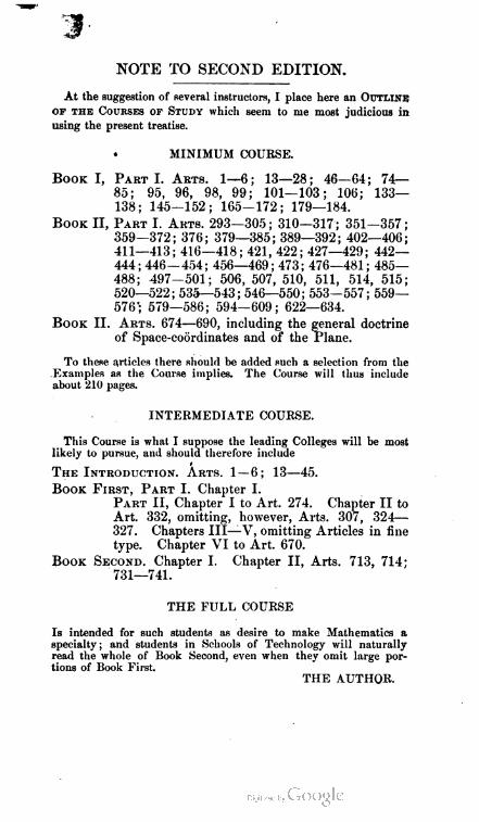
At the suggestion of several instructors, I place here an OUTLINE
or the Courses of Study which seem to me most judicious in
using the present treatise.
• MINIMUM COUESE.
Book I, Part I. Arts. 1—6; 13—28; 46—64 ; 74—
85; 95, 96, 98, 99; 101—103; 106; 133—
138; 145—152; 165—172; 179—184.
Book II, Part I. Arts. 293—305; 310—317 ; 351—357;
359—372; 376; 379—385; 389—392; 402—406;
411—413; 416—418; 421, 422; 427—429; 442—
444; 446— 454; 456—469; 473; 476—481; 485—
488; 497-501; 506, 507, 510, 511, 514, 515;
520—522; 535—543 ; 546—550 ; 553—557; 559—
576'; 579—586; 594-609; 622—634.
Book II. Arts. 674—690, including the general doctrine
of Space-coordinates and of the Plane.
To these articles there should be added such a selection from the
Examples as the Course implies. The Course will thus include
about 210 pages.
INTEEMEDIATE COUESE.
This Course is what I suppose the leading Colleges will be most
likely to pursue, and should therefore include
i
The Introduction. Arts. 1 — 6; 13—45.
Book First, Part I. Chapter I.
Part II, Chapter I to Art. 274. Chapter II to
Art. 332, omitting, however, Arts. 307, 324—
327. Chapters III—V, omitting Articles in fine
type. Chapter VI to Art. 670.
Book Second. Chapter I. Chapter II, Arts. 713, 714;
731—741.
THE PULL COUESE
Is intended for such students as desire to make Mathematics a
specialty ; and students in Schools of Technology will naturally
read the whole of Book Second, even when they omit large por
tions of Book First.
THE AUTHOB.

ERRATA.
Page 63, line 20 : for sin — at read sin,a>.
" 103, " 21: for + read = .
" 103, " 22 : dele the period at the close.
" 221, " 24: for k"=A:sinCrendk"=sinA:sinC.
" 247, " 9 : put the 2 outside of the brace.
" 269, " 28 : for of read to, and dele the period.
CONTENTS.
INTRODUCTION:—THE NATURE, DIVISIONS, AND
METHOD OF THE SCIENCE.
PAGE.
I. Determinate Geometry:
Principles of Notation, 5
Examples-, .......... 8
Principles of Construction, 8
Examples, 16
Determinate Problems :
In a given triangle, to inscribe a square, .... 16
" " " " a rectangle with sides in given
ratio, ..... 17
To construct a common tangent to two given circles, . . 18
" a rectangle, given area and difference of sides, . 21
Examples, 23
II. Indeterminate Geometry :
1°. Development of its Fundamental Principle :
The Convention of Co-ordinates, .... 26
Distinction between Variables and Constants; defi
nition of a Function, . . . . 28
Equations between co-ordinates : their geometric
moaning, 29
The Locus denned and illustrated, .... 33
11°. Its Method outlined; in what sense it is Analytic:
Manner of employing geometric equations to estab
lish properties, 35
Special analytic character of the Algebraic Calculus, 38
Elements of analysis added by the Convention of Co
ordinates, ....... 39
111°. Its Divisions and Subdivisions :
Algebraic and Transcendental Geometry, ... 41
Orders of algebraic loci : Elementary and Higher
Geometry, 42
Loci in a Plane and in Space: Geometry of Two and
of Three Dimensions, 42
(v)
vi CONTENTS.
BOOK FIRST:—PLANE CO-OEDINATES.
Part I. On the Representation of Form by Analytic
Symbols.
CHAPTER FIRST.
THE OLDER GEOMETRY: BILINEAR AND POLAR CO-ORDINATES.
Section I.—The Point. PA0K
Bilinear Or Cartesian System op Co-ordinates : Explanation in
detail, 48
Expressions for Point on either Axis; — for the Origin,. . 50
Polar System op Co-ordinates : 52
Expression for the Pole; — for Point on Initial Line, . . 53
Distance, in both systems, between any Two Points in a plane, . 55
Co-ordinates of Point cutting this distance in a given ratio, . . 56
Transformation of Co-ordinates :
I. To change the Origin, Axes remaining parallel to their
first position, 59
II. To change the Inclination of the Axes, Origin remaining
the same, ........ 59
Particular Cases: — 1. From Rectangular Axes to
Oblique, ... 60
2. From Oblique to Rectangular, 61
3. From Rectangular to Rect
angular, .... 61
III. To change System— from Bilinears to Polars, and con
versely, 62
IV. To change the Origin, and make either previous Trans
formation at the same time, ..... 63
General Principles op Interpretation :
I. Any single equation between co-ordinates represents a
Locus, 65
II. Any two simultaneous equations represent Determinate
Points, ........ 67
III. Any equation lacking absolute term, represents Locus
passing through Origin, ..... 69
IV. Transformation of Co-ordinates does not affect Locus, nor
change the Degree of its Equation, ... 69
Special Interpretation of Equations : Tracing their Loci by
means of Points, 71
Definitions and illustrations, 72
Examples: — Equations to some of the Higher Plane Curves, 75

CONTENTS. vii
Section II.— The Eight Line.
A. THE RIGHT LINE UNDER GENERAL CONDITIONS.
I. Geometric Point of View:—Equation to Right Line is always of
the First Degree. pack.
Equation in terms of angle made by Line with axis X, and of its
intercept on axis Y, 79
" " its intercepts on the two axes, ... 81
" " its perpendicular from the Origin, and angle
of perp'r with axis X, . . . .83
Polar equation, deduced geometrically, 84
II. Analytic Point of View: — Every equation of First Degree in two
variables represents a Right Line.
Proof of the theorem by Algebraic Transformation of the general
equation of First Degree, ....... 87
Proof by means of the Trigonometric Function implied in the equation, 87
Proof by Transformation of Co-ordinates, 89
Analytic deduction of the Three Forms of the equation, . . 92
Reduction of Ax + By + C= 0 to the form x cos a + y cos 0 — p = 0, . 95
Polar Equation obtained by Transformation of Co-ordinates, . . 97
B. THE RIGHT LINE UNDER SPECIAL CONDITIONS.
Equation to Right Line passing through Two Fixed Points, . 98
Angle between two Right Lines : condition that they shall be
parallel or perpendicular, ....... 100
Equation to Right Line parallel to given Line ; — perpendicular to
given Line, .......... 101
Equation to Right Line passing through given Point, and parallel
to given Line, 103
Equation to any Right Line through a Fixed Point, . . 103
Equation to Right Line through a given Point, and cutting a given
line at given angle, 105
Equation to Perpendicular through a given Point, . . . 106
Length of Perpendicular from {x,y) on x cos o + ycos 0—p= 0 ; also
on Ax + By + C=0, 107
Equation to any Right Line through the intersection of two given ones, 109
Meaning of equation L + IcL1 = 0, 110
Equation to Bisector of angle between any two Right Lines, . . 113
Equation to the Right Line situated at Infinity, .... 116
Equations of Condition :
Condition that Three Points shall lie on one Right Line, . . 117
" " Three Right Lines shall meet in One Point, . 118
" " Movable Right Line shall pass through a Fixed
Point, 118

viii CONTENTS.
C. EXAMPLES ON THE RIGHT LINE. pAQE
Examples in Notation and Conditions, 120
Examples of Rectilinear Loci, 125
Section III.— Pairs of Right Lines.
I. Geometric Point of View:—Equation to a Pair of Right Lines
is always oj Second Degree.
Formation of equations in the type of LMN ....=■ 0 : their con
sequent meaning, ........ 130
Interpretation of equation LL'= 0, ..... 130
Equation to Pair of Right Lines passing through a Fixed Point, . 131
Meaning of the equation Ax1 + 2Hxy + By' = 0, . . . 132
Angle between the Pair Ax' + 2Hxy + By' = 0, . . . . 133
Condition that they shall cut at right angles, .... 134
Equation to Bisectors of angles between Ax' + 2Hxy + By' = 0, . 134
Case of Two Imaginary Lines having Real Bisectors of their
angles, 134
II. Analytic Point of View:—The Equation of Second Degree in
two variables, upon a Determinate Condition, represents Two
Might Lines.
Proof of the theorem by the mode of forming LL' = 0, . . . 135
Condition on which Ax* + IHxy + By1 + 2Gx + 2Fy + C'= 0 repre
sents Two Right Lines, 136
Section IV.—The Circle.
I. Geometric Point of View : —Equation to Circle is always of Sec
ond Degree.
Equation to the Circle, referred to any Rectangular Axes, deduced
from geometric definition, . 138
tt tt tt (< Oblique Axes, .... 139
tt tt tt tt Rectangular Axes with Origin at
139
li tt tt tt Diameter and Tangent at its
extremity, .... 140
Polar Equation to the Circle, 140
1 1. Analytic Point of View : — The Equation of Second Degree in two
variables, upon a Determinate Condition, represents a Circle.
Proof of theorem by comparison of the General Equation with that
to Circle, 142

CONTENTS. ix
PAGE.
Condition that 4a? + 2Hxy + By* + 2Gx + 2Fy + C= 0 shall rep
resent a Circle, 143
To determine Magnitude and Position of Circle, given its equa
tion, ............ 144
Condition that a Circle shall touch the Axes, 145
Examples, 146
Section V. —The Ellipse.
I. Geometric Point of View: —Equation to Ellipse is always of Sec
ond Degree.
Equation to the Ellipse deduced from geometric definitions, . . 149
Its general Form, referred to Axes of Curve and Focal Center, . 150
Center of a Curve defined : proof that Focal Center is center of the
Ellipse, 151
Polar Equation to Ellipse, Center being Pole, ..... 151
" " " Focus " " 153
II. Analytic Point of View:—The Equation of Second Degree in two
variables, upon a Determinate Condition, represents an Ellipse.
Reduction of Ax2 + 2Hxy + Bu2 + 2 Gx + 2Fy+ C= 0 to Center of its
Locus, 155
Condition that it represent an Ellipse is H2 — AB<.0, . . . 159
The Point, as intersection of Two Imaginary Right Lines, a partic
ular case of the Ellipse, . . . . . . . . 161
Examples, 165
Section VI.—The Hyperbola.
I. Geometric Point of View:—Equation to Hyperbola is always of
Second Degree.
Equation to the Hyperbola deduced from geometric definitions, 169
Its general Form, referred to the Axes and Focal Center, . 170
Proof that the Focal Center is the center of the Hyperbola, . 172
Polar Equation to Hyperbola, Center being Pole, .... 172
" " " " Focus " " .... 174
II. Analytic Point of View: —The Equation of Second Degree in two
variables, upon a Determinate Condition, represents an Hyperbola.
Equation to Hyperbola compared with Reduced Equation of Second
Degree, ........ 175
Condition that the latter shall represent an Hyperbola is
H'-AB>0, 176
Two Right Lines intersecting, a particular case of the Hyperbola, . 177
x CONTEXTS.
PAGE.
Examples on the Hyperbola, 178
Section VII.—The Parabola.
I. Geometric Point of View: — Equation to Parabola is always of
Second Degree.
Equation to Parabola deduced from geometric definitions, . . 181
Its general Form, referred to Axis and Directrix, . . . 182
Polar Equation to Parabola, Focus being Pole, .... 183
II. Analytic Point of View : — The Equation of Second Degree in two
variables, upon a Determinate Condition, represents a Parabola.
Additional transformation of General Equation, under condition of
non-centrality, .......... 185
Condition that it represent a Parabola is H* — AB = 0, . . . 188
The Right Lino as Center of Two Parallels, .... 189
" " " as Limit of Two Parallels, a particular case of
the Parabola, 190
Examples, ........... 191
Section VIII.—Locus of Second Order in General.
Summary of Conditions already imposed upon the General Equa
tion, ............
Proof that these exhaust the varieties of its Locus,
Conies defined : Classification into Three Species, ....
Resume of argument for the theorem : Every Equation of the Second
Degree in two variables, represents a Conic, ....
CHAPTER SECOND.
THE MODERN GEOMETRY :-TRILINEAR AND TANGENTIAL
CO-ORDINATES.
Section I. — Trilinear Co-ordinates.
Trilinear Method of representing a Point, ..... 199
Origin of the Method: the Abridged Notation, .... 200
Geometric meaning of the constant k in a + k(3 = 0, . . . . 201
Interpretation of the equations a ± kff= 0, a ± 0= 0, . . . 201
The Notation extended to equations in the form Ax + By + C= 0, . 202
Meaning of the equation la + mfl -f ny = 0 : condition that it repre
sent any Right Line, ........ 203
Examples : Any line of Quadrilateral, in terms of any Three, . 206
190
197
197
CONTENTS. xi
PAGE.
The symbols a, ft, y may be considered as Co-ordinates, . . . 207
Peculiar Nature of Trilinear Co-ordinates : each a Determined Func
tion of the other two, 208
Equation expressing this Condition is aa + hff + cy = M, . . 209
General trilinear symbol for a Constant ; namely, k [a sin A +
IS sin B + y sin C), 210
To render homogeneous any given equation in Trilinears, . . 210
Trilinear Equation to Right Line, 212
" " " " parallel to a given one, . . 212
" " " " situated at infinity, . . .212
Condition, in Trilinears, that two Right Lines shall be at right angles
to each other, . . . . . . . . . .213
Trilinear Equation to Right Line joining Two Fixed Points, . . 214
" " any Conic, referred to Inscribed Triangle, . 215
" " Circle, " " " . . 216
Same for any Concentric Circle, . . 216
" " " Triangle of Reference having any sit
uation, ....... 217
General Equation of Second Degree in Trilinears : i. e., Trilinear
Equation to any Conic, Triangle of Reference having any sit
uation, 218
Trilinear Equations to Chord and Tangent of any Conic, . . . 219
Examples of Trilinear Notation and Conditions, . . . 220
Section II.—Tangential Co-ordinates.
In Tangential system, Lines are represented by co-ordinates, and
Points by equations, ........ 225
Cartesian Co-efficients are Tangential Co-ordinates : Tangential Equa
tions are Cartesian Equations of Condition— namely, that a
Line shall pass through two Consecutive Points on a given
Curve, 225
Geometric interpretation of Tangentials : how they represent a Locus.
Reason for Name, ......... 226
The Right Line in the Tangential System, 227
Envelopes defined : Condition that a Right Line shall touch a Curve
is the Tangential equation to the Curve ; or simply the Equa
tion to the Envelope of the Line, ...... 228
Development of the Tangential Equation to a Conic, referred to In
scribed Triangle, 228
Reciprocal relation between Points and Lines : the Principle of
Duality, 235
Description of the Method of Reciprocal Polars : its relation to the
Modern Geometry 238
Examples illustrating Tangentials, ...... 242
Xll CONTENTS.
Part II. Ox the Properties of Conics.
CHAPTER FIRST.
THE RIGHT LINE.PAGE.
Area of a Triangle in terms of the Co-ordinates of its vertices, . 246
" " " given the Right Lines which inclose it, . . 246
Compound ratio of segments of the Three Sides by any Trans
versal = - 1, 248
Compound ratio of segments of the Three Sides by any three Con-
vergents = + 1, . . . . . . . . . 248
Various cases of Three Convergents occurring in any Triangle,
solved by the Abridged Notation, 249
Further application of Trilinears : The property of Homology ;
Axis and Center of Homology, ...... 250
Quadrilaterals — when Complete: Centers of their three Diagonals
lie on one Right Line, 251
Harmonic and Anharmonic Properties:...... 253
Constant ratio among Segments of Transversals to any Linear
Pencil, 253
Harmonic and Anharmonic Pencils, ...... 254
k
V
a, /?, a -I- fc/J, a — k@, form a Harmonic Pencil, .... 255
Anharmonic of any Pencil a + kfi, a + 10, a + m0, a + n0 =
(«-&)("'- 0 25,
(u-m) (l-k)'
Definition of Homographic Systems of lines, .... 257
Examples involving properties of the Right Line:
Triangles, 257
Harmonics of a Complete Quadrilateral, 258
Anharmonic of a, 0, a + k0, a + k'0 = — , 255
CHAPTER SECOND.
THE CIRCLE.I. The Axis op X:
Every Ordinate a mean proportional between the correspond
ing segments, ........ 259
Every Right Line meets the Curvo in Two Points, . . 260
Discrimination between Real, Coincident, and Imagi
nary points, 2R0
Chords defined. Equation to any Chord, .... 262
II. Diameters :
Definition : Locus of middle points of Parallel Chords.
Equation, 263
CONTENTS. xiii
Every diameter passes through Center, and is perpendicular
to bisected Chords, ....... 264
Conjugate Diameters defined — each bisects Chords parallel
to the other, ........ 264
Conjugates of the Circle are at right angles, . . . 205
III. Tangent :
Definition : Chord meeting Curve in Two Coincident Points, 265
Equation, 266
Condition that a Right Line shall touch Circle. Auxiliary
Angle, 267
Analytic Construction of Tangent through (x',y'): Two Tan
gents, real, coincident, or imaginary, .... 268
Length of Tangent from (x, y) = V'S, 269
Subtangent— its definition and value, .... 270, 271
IV. Normal:
Definition of Normal. Equation, 270
The Normal to Circle passes through Center. Length con
stant, 271
Subnormal— its definition and value, 271
V. Supplemental Chords :
Definition : Equation of Condition, .... 271, 272
In the Circle, they are always at right angles, . , . 272
VI. Pole and Polar:
Development of the conception of the Polar, .... 273
I. Chord of Contact to Tangents from (x' , y'), . . 273
II. Locus of intersection of Tangents at extremities of
convergent chords, ...... 273
III. Tangent brought under this conception, . . . 274
Construction of Polar from its definition, .... 276
Polar is perpendicular to Diameter through Pole : — its dis
tance from Center, ....... 277
Simplified geometric construction, 277
Distances of any two points from Center are proportional to
distance of each from Polar of the other, . . . 278
Conjugate and Self-conjugate Triangles defined: — they are
homologous, 278, 279
SYSTEMS OF CIRCLES.
I. System with Common Radical Axis:
Radical Axis defined: its Equation, S—S' = 0, . . . 280
It is perpendicular to the line of the centers, . . . 281
Construction : Combine ft — S1 - 0 with y — 0 and observe
the foregoing, 281
The three Radical Axes belonging to any three Ciroles meet
in one point: Radical Center, • . 281

xiv CONTENTS.
PAGE.
To construct the Radical Axis by means of tho Radical
Center, 281
Radical Axis of Point and Circle ; — of Two Points, . . 282
Definition of System of Circles with Common Radical Axis ; —
Their Centers lie on one Right Line. Their Equa
tion: x2 + f-2kx±P = 0, 282
To trace the System from the equation, 283
Locus of Contact of Tangents from any point in the C. R. A.
is Orthogonal Circle, 283
Geometric construction of the System : Limiting Points, 284
Analytic proof of the existence of the Limiting Points, . 285
II. Two Circles with Common Tangent :
To determine the Chords of Contact, 287
The Tangents intersect on Line of Centers, and cut it in ratio
of Radii, 289
Every Right Line through these Points of Section is cut sim
ilarly by the two Circles, ...... 289
The Centers of Similitude, 289
The three homologous Centers of Similitude belonging to any
three Circles, lie on one Right Line. The Axis of
Similitude 290
THE CIRCLE IN THE ABEIDGED NOTATION.
If a Triangle be inscribed in a Circle, and Perpendiculars be dropped
from any point in the Circle upon the three sides, their feet
will lie on one Right Line, 291
Angle between Tangent and Chord = angle inscribed under corre
sponding arc, .......... 292
Trilinear Equation to tho Tangent, referred to Inscribed Triangle, . 292
Tangents at Vertices of Inscribed Triangle cut Opposite Sides
in points lying on one Right Line, ..... 292
Lines joining Vertices of Inscribed Triangle to those of Tri
angle formed by Tangents meet in one Point, . . 292
Radical Axis in Trilinears, 293
Examples on the Circle, 293
CHAPTER THIRD.
THE ELLIPSE.
I. The Curve referred to its Axes.
THE AXES.
Theorem I. Focal Center bisects the Axes. Corresponding inter-
pretation of — + ^ = 1, ...... 297r a' b2 '

CONTENTS. XV
PAGE.
Theorem II. Foci fall within the Curve, 298
Theorem III. Vertices of Curve equidistant from Foci, . . 298
Theorem IV. Sum of Focal Radii = length of Transverse Axis. To
construct Curve by Points, 298
Theorem V. Semi-conjugate Axis a geometric mean between
Focal Segments of Transverse, .... 299
Cor. Distance from Focus to Vertex of Conjugate =
Semi-transverse. To construct Foci, . . . 299
Theorem VI. Squares of Ordinates to Axes are proportional to
Rectangles of corresponding Segments, . . 300
Cor. The Labia Rectum, and its value, . . . 300
Theorem VII. Squares of Axes are to each other as Rectangle of
any two segments to Square of Ordinate, . . 301
Theorem VIII. Ordinate of Ellipse : Corresponding Ordinate of
Circumscribed Circle : : Semi-conjugate : Semi-
transverse, 301
Cor. 1. Analogous relation to Inscribed Circle. Con
structions for the Curve, 302
a2 — VCor. 2. Interpretation of -— = e2 : e defined as
the Eccentricity, 303
Theorem IX. The Focal Radius of the Curve is a Linear Function
of corresponding Abscissa, 304
Linear Equation to Ellipse : p = a ± ex, . . 304
Verification of the Figure of the Curve by means of its equation, . 304
DIAMETERS.
Diameters : Equation to Locus of middle points of Parallel
Chords, 305
Theorem X. Every Diameter is a Right Line passing through
the Center, 306
Cor. Every Right Line through Center is a Diam
eter, 306
Theorem XI. Every Diameter of an Ellipse cuts Curve in Two
Real Points, .... . 306
Length of Diameter, in the Ellipse, 306
Theorem XII. Transverse Axis the maximum, and Conjugate the
minimum Diameter, ...... 306
Theorem XIII. Diameters making supplemental angles with Axis
Major are equal, ....... 307
Cor. Given the Curve, to construct the Axes, . . 307
Theorem XIV. If a Diameter bisects Chords parallel to a second,
second bisects Chords parallel to first, . . 307
Conjugate Diameters defined: Ordinates to any Diameter, . . 308
To construct a pair of Conjugates, .... 308
XVI CONTEXTS.
PAGE.
Equation of Condition to Conjugates, in the Ellipse, is
b'tan d. tan 8' = = , 308
a
Theorem XV. Conjugates in the Ellipse lie on opposite sides of
Axis Minor, 308
Equation to Diameter Conjugate to that through any given point, . 309
Cor. The Axes are a case of Conjugates, . . 309
(liven the co-ordinates to extremity of any Diameter, to find those
to extremity of its Conjugate, ...... 309
Theorem XVI. Abscissa to extremity of Diameter : Ordinate to
extremity of its Conjugate : : Axis Major :
Axis Minor, 310
Theorem XVII. Sum of squares on Ordinates to extremities of
Conjugates, constant and = V, . . 310
Length of any Diameter in terms of Abscissa to extremity of its
Conjugate, .......... 310
Theorem XVIII. Square on any Semi-diameter = Rectangle Focal
Radii to extremity of its Conjugate, . . 311
Theorem XIX. Distance, measured on a Focal Chord, from ex
tremity of any Diameter to its Conjugate, is
constant, and equals the Semi-Major, . . 311
Theorem XX. Sum of squares on any two Conjugates is constant
and = sum squares on Axes, . . . 312
Angle between any two Conjugates, . . . 312
Theorem XXI. Parallelogram under any two Conjugates, constant
and = Rectangular under Axes, . . . 313
Cor. 1. Curve has but one set of Rectangular Con
jugates, ........ 313
Cor. 2. Inclination of Conjugates is maximum
when a' = b', 314
Theorem XXII. Equi-conjugates : they are the Diagonals of Cir
cumscribed Rectangle, ..... 314
Cor. Curve has but one pair of Equi-conju
gates, ........ 314
Anticipation of the Asymptotes in the Hyperbola, .... 315
THE TANGKNT.
Equation to the Tangent, referred to the Axes, .... 315
Condition that a Right Line touch an Ellipse. Eccentric Angle, . 316
Analytic construction of the Tangent through any point : Two,
real, coincident,or imaginary, ...... 317
Theorem XXIII. Tangent at extremity of any Diameter is parallel
to its Conjugate, 318
Cor. Tangents at extremities of any Diameter arc
parallel. Circumscribed Parallelogram, . 318

CONTENTS. xvii
PAGE.
Theorem XXIV. Tangent bisects the External Angle between
Focal Radii of Contact, .... 319
Cor. 1. To construct a Tangent to the Ellipse at
a given point, ...... 319
Cor. 2. Derivation of the term Focue, . . 319
Intercept by Tangent on Axis Major: Constructions for Tangent
by means of it, ......... 320
The Subtangent defined: Distinction between Subtangent of the
Curve and of a Diameter, 320
Theorem XXV. Subtangent of Curve is Fourth Proportional to
Abscissa of Contact and the corresponding
segments of Axis Major, .... 321
Cor. Construction of Tangent by means of Cir-
cumser. Circle : Subtan. not function of b, . 321
Theorem XXVI. Perpendicular from Center on Tangent is Fourth
Proportional to the corresponding Semi-
conjugate and the Semi-axes : p = ~ , . 322
Length of the Central Perp'r in terms of its angles with the Axes, . 322
Theorem XXVII. Locus of Intersection of Tangents cutting at
right angles is Concentric Circle, . . 323
Focal Perpendiculars upon Tangent: their length, .... 323
Theorem XXVIII. Focal Perpendiculars on Tangent are propor
tional to adjacent Focal Radii, . . . 324
Theorem XXIX. Rectangle under Focal Perpendiculars, constant
and = b', 324
Theorem XXX. Locus of foot of Focal Perpendicular is the Cir
cumscribed Circle, 324
Cor. Method of drawing the Tangent, common
to all Conies, 325
Theorem XXXI. If from any Point within a circle a Chord be
drawn, and a perpendicular to it at the
point of section, the Perpendicular is Tan
gent to an Ellipse, 326
Cor. The Ellipse as Envelope, .... 326
Theorem XXXII. Diameters through feet of Focal Perpendiculars,
parallel to Focal Radii of Contact, . . 327
Cor. Diameters parallel to Focal Radii of Con
tact, meet Tangent at the feet of the Focal
Perpendiculars, and are of the constant
length = 2n, 327
THE NORMAL.
Equation to the Normal, referred to the Axes, • 328
Theorem XXXIII. Normal bisects the Internal Angle between Focal
Radii of Contact, 328
An. Ge. 2.
XV111 CONTENTS.
PAGE.
Cor. 1. To construct a Normal at given point
on the Ellipse, 329
Cor. 2. To construct a Normal through any
point on Axis Minor, .... 329
Intercept of Normal on Axis Major : Constructions by means of it, 329
Theorem XXXIV. Normal cuts distance between Foci in segments
proportional to adjacent Focal Radii, . 330
The Subnormal denned : Subnormal of the Curve — its length, . 330
Theorem XXXV. Normal cuts its Abscissa in constant ratio =
—' 330
Length of Normal from Point of Contact to either Axis, . . 330
Theorem XXXVI. Rectangle under Segments of Normal by Axes =
Square on Conjugate Semi-diameter, . 331
Cor. Equal, also, to Rectangle under corre
sponding Focal Radii, .... 331
Theorem XXXVII. Rectangle under Normal and Central Perpen
dicular, constant and = a2, . . . 331
SUPPLEMENTAL, AND FOCAL CHORDS.
Equation of Condition to Supplemental Chords, .... 332
Theorem XXXVIII. Diameters parallel to Supplemental Chords are
Conjugate, 332
Cor. 1. To construct Conjugates at a given in
clination. Caution, ..... 333
Cor. 2. To construct a Tangent parallel to
given Right Line, 333
Cor. 3. To construct the Axes in the empty
Curve, 333
Focal Chords — Special Properties, 334
Theorem XXXIX. Focal Chord parallel to any Diameter, a third
proportional to Axis Major and the Di
ameter, 335
II. The Curve referred to any Two Conjugates.
DIAMETRAL PROPERTIES.
Equation to Ellipse, referred to Conjugates, 336
Theorem XL. Squares on Ordinatcs to any Diameter, proportional
to Rectangles under corresponding Segments, 337
Theorem XLI. Square on Diameter : Square on Conjugate : : Rect
angle under Segments : Square on Ordinate, . 337
Theorem XLII. Ordinate to Ellipse : Corresponding Ordinate to
Circle on Diameter : : b' : o', . . . 338
Cor. 1. Given a pair of Conjugates, to construct
the Curve, 338

CONTENTS. xix
PAGE.
Cor. 2. General interp'n of x2 + y* = an : Ellipse,
referred to Equi-conjugates, ... . 339
Figure of the Ellipse with respect to any two Conjugates, . . 339
CONJUGATE PROPERTIES OF THE TANGENT.
Equation to Tangent, referred to Conjugates, 339
Theorem XLIII. Intercept of Tangent on any Diameter, third
proportional to Abscissa of Contact and the
a"Semi-diameter : x = — , . . . . 340
Theorem XLIV. Rectangle under Intercepts by Variable Tangent
on Two Fixed Parallel Tangents, constant
and = Square on parallel Semi-diameter, . 341
Theorem XLV. Rectangle under Intercepts on Variable Tangent
by Two Fixed Parallel Tangents, variable
and = Square on Semi-diameter parallel to
Variable, 341
Theorem XLVI. Rectangle under Intercepts on Variable Tangent
by any two Conjugates equals Square on
Semi-diameter parallel to Tangent, . . 342
Cor. 1. Diameters through intersections of Va
riable Tangent with Two Fixed Parallel
ones, are Conjugate, ..... 342
Cor. 2. Given two Conjugates in position and
magnitude, construct the Axes, . . . 342
an — x'1
The Subtangent to ant Diameter: its length = ;— , . . 343x
Cor. Construction of Tangent by means of
Auxiliary Circle, 343
Theorem XLVII. Rectangle under Subtangent and Abscissa of
Contact : Square on Ordinate : : an ■ b", . 344
Theorem XLVIII. Tangents at extremities of any Chord meet on
its bisecting Diameter, .... 345
PARAMETERS.
Parameter to any Diameter denned : Third proportional to Diam
eter and Conjugate, - 345
Parameter of the Curve : identical with Latus Rectum, . . . 345
Theorem XLIX. In the Ellipse, no Parameter except the Princi
pal is equal in value to the Focal Double
Ordinate, 346
THE POLE AND THE POLAR.
Development of the Equation to the Polar : Definition, . . 346—349
Cor. Construction of Pole or Polar from its
definition, 349

XX CONTENTS.
PAGE.
Theorem L. Polar of any Point, parallel to Diameter Conjugate
to the Point, 350
Special Properties : Polar of Center ; — of any point on axis of x ; —
on Axis Major, 350
Cor. Second geometric construction for Polar, . 351
Polar op Focus : its distance from center, and its direction, . . 351
Theorem LI. Ratio between Focal and Polar distances of any
point on Ellipse, constant and = e, . . 352
Cor. 1. On the construction of the Ellipse according
to this theorem, 352
Cor. 2. Polar of Focus hence called the Directrix, . 353
Cor. 3. Second basis for the name Ellipse, . . 353
Theorem LII. Line from Focus to Pole of any Chord, bisects focal
angle which the Chord subtends, . . . 354
Cor. Line from Focus to Pole of Focal Chord, per
pendicular to Chord, 354
III. The Curve referred to its Foci.
Interpretation of the Polar Equations to the Ellipse, . . . 355
Development of the Polar Equation to a Tangent, .... 355
Polar proof of Theorem XIX compared with former proof, and with
that by pure Geometry, 356
IV. Area of the Ellipse.
Theorem LIII. Area of Ellipse = ir times the Rectangle under its
Semi-axes, 358
V. Examples on the Ellipse.
Loci, Transformations, and Properties, ...... 358
CHAPTER FOURTH.
THE HYPERBOLA.
I. The Curve referred to its Axes.
THE AXES.
Theorem I. Focal Center bisects the Axes. Corresponding inter-
pretation of — ^ = 1, 363
The Axis Conjugate, conventional: Equation to the Conjugate Hy
perbola, 364
Theorem II. Foci full without the Curve, 365
Theorem III. Vertices of Curve, equidistant from Foci, . . 365
Theorem IV. Difference Focal Radii = Transverse. The Curve by
Points, 365
\
CONTENTS. xxi
PACK.
Theorem V. Conventional Semi-conjugate, geometric mean be
tween Focal Segments of Transverse, . . 366
Cor. Dist. from Center to Focus = dist. between ex
tremities of Axes. To construct Foei, . . 366
Theorem VI. Squares on Ordinates to Axes, proportional to Rect
angles under corresponding Segments, . . 367
Cor. The Latua Rectum, and its value, . . . 367
Theorem VII. Squares on Axes are as Rectangle under any two
Segments to Square on their Ordinate, . . 367
Analogy of Hyperbola to Ellipse, with respect to Circle on Trans
verse, defective. Circle replaced by the Equilateral Hyperbola, 368
Theorem VIII. Ordinate Hyperbola : Corresponding Ordinate of its
Equilateral :: b : a, 368
„ a'+ b2Cor. Interpretation of i— = e2. e defined as the
Eccentricity, ....... 369
Theorem IX. Focal Radius of Curve, a LinearFunction of corre
sponding Abscissa, 370
Linear Equation to Hyperbola: p=ex±a, . . 371
Verification of Figure of Curve by means of its equation, . . 371
DIAMETERS.
Diameters : Equation to Locus of middle points of Parallel Chords, 371
Theorem X. Every Diameter a Right Line passing through the
Center, 371
Cor. Every Right Line through center is a Diam
eter, 372
Theorem XI. " Every Diameter cuts Curve in Two Real Points "
untrue for Hyperbola, 372
Cor. 1. Limit of those diameters having real intersec
tions: fl=tan-'-, 372a
Cor. 2. All diameters cutting Hyperbola in Imagi
nary Points, cut its Conjugate in Two Real ones, 373
Length of Diameter, in the Hyperbola, ...... 373
Theorem XII. Each Axis the minimum diameter for its own curve, . 373
Theorem XIII. Diameters making supplemental angles with Trans
verse are equal, 374
Cor. Given the Curve, to construct the Axes, . . 374
Theorem XIV. If a Diameter bisects Chords parallel to a second,
second bisects those parallel to first, . . 374
Conjugate Diameters : Ordinates, 374
To construct a pair of Conjugates, .... 374
6!Equation of Condition to Conjugates, in Hyperbola ; tan 0. tan 8' = —2 > 375

XXII CONTENTS.
PAGE.
Theorem XV. Conjugates in the Hyperbola lie on same side of
Conjugate Axis, 375
Equation to Diameter Conjugate to that through any given point, . 375
Cor. The Axes are a case of Conjugates, . . 376
Given co-ordinates to extremity of Diamoter, to find those to ex
tremity of its Conjugate, ........ 376
Theorem XVI. Abscissa ext'y of any Diameter : Ordinate ext'y
of its Conjugate : : Transverse : Conjugate,
Theorem XVII. Din", squares on Ordinates to extremities of Con
jugates, constant and = If,
Length of any Diameter in terms of Abscissa to extremity of its
Conjugate, ..........
Theorem XVIII. Square on any Semi-diameter = Rectangle Focal
Radii to extremity of its Conjugate,
Theorem XIX. Distance, measured on Focal Chord, from extrem
ity of any Diameter to its Conjugate, constant
and equal to Semi-Transverse,
Theorem XX. Difference of squares on any two Conjugates, con
stant and = difference of squares on Axes,
Anglo between any two Conjugates,
Theorem XXI. Parallelogram under any two Conjugates, constant
and = Rectangular under Axes,
Cor. 1. Curve has but one set of Rectangular
Conjugates, ....... 380
Cor. 2. Inclination of Conjugates diminishes with
out limit : the conception of Equi-conjugates
replaced by that of Self-conjugates,
Theorem XXII. The Self-conjugates in the Hyperbola are Diago
nals of the Inscribed Rectangle, .
Cor. Curve has two, and but two, Self-conjugates,
Analogy of the Self-conjugates to the Equi-conjugates of the Ellipse,
376
376
377
378
378
378
379
379
380
381
381
382
THE TANGENT.
Equation to Tangent, referred to the Axes, 382
Condition that a Right Line touch an Hyperbola. Eccentric Angle, . 383
Analytic construction of the Tangent through any point : Two, real,
coincident, or imaginary, 384
Theorem XXIII. Tangent at extremity of any Diameter, parallel
to its Conjugate, ...... 385
Cor. Tangents at extremities of any Diameter are
parallel. To circumscribe Parallelogram, . 385
Theorem XXIV. Tangent bisects the Internal Angle between Focal
Radii of Contact, 386
Cor. 1. To construct Tangent to Hyperbola, at a
given point, ....... 386
Cor. 2. Derivation of the term Focus, . . . 386
V

CONTENTS. xxin
PAGE.
Intercept by Tangent on the Transverse Axis : Constructions by
means of it, 387
The Subtangent to the Hyperbola 387
Theorem XXV. Subtangent of Curve a Fourth Proportional to
Abscissa of Contact and corresponding seg
ments of Transverse, ..... 387
Cor. 1. Defect supplied in the analogy between
Hyperbola and Ellipse, respecting Circle
on 2a, 388
Cor. 2. Construction of Tangent by means of
Inscribed Circle, 388
Theorem XXVI. Central Perpendicular on Tangent, a Fourth Pro
portional to corresponding Semi-conjugate
and the Semi-axes : p = ~ , . . . 389
Length of Central Perpendicular in terms of its angles with Axes, . 389
Theorem XXVII. Locus of Intersection of Tangents cutting at
right angles is Concentric Circle, . . 390
Focal Perpendiculars on Tangent: their length, .... 390
Theorem XXVIII. Focal Perpendiculars proportional to adjacent
Focal Radii, 390
Theorem XXIX. Rectangle under Focal Perpendiculars, constant
and = b2, ... 391
Theorem XXX. Locus of foot of Focal Perpendicular is In
scribed Circle, 391
Cor. To draw Tangent by the method common
to all Conies, 391
Theorem XXXI. If, from any point without a Circle, a Chord be
drawn, and a perpendicular to it at the
point of section, the Perpendicular is Tan
gent to an Hyperbola, .... 392
Cor. The Hyperbola as Envelope, . . . 392
Theorem XXXII. Diameters through feet of Focal Perpendiculars
are parallel to Focal Radii of Contact, . 393
Cor. Diameters parallel to Focal Radii of Con
tact, meet Tangent at the feet of Focal
Perpendiculars, and are of the constant
length = 2a, 393
THE NORMAL.
Equation to the Normal, referred to the Axes, ..... 393
Theorem XXXIII. Normal bisects the External Angle between
Focal Radii of Contact, .... 394
Cor. 1. If Ellipse and Hyperbola are confocal,
Normal to one is Tangent to other at inter
section, 394
xxiv CONTENTS.
PAGE.
Cor. 2. To construct Normal at any point on
Hyperbola, 394
Cor. 3. To construct Normal through any
point on Conjugate Axis, . . . 394
Intercept of Normal on Transverse Axis : Constructions by means
of it, 395
Theorem XXXIV. Normal cuts distance (produced) between Foci
in segments proport'l to Focal Radii, . 395
The Subnormal : Subnormal of the Hyperbola—its length, . . 396
Theorem XXXV. Normal cuts its Abscissa in the constant
a? + V-ratio = —— , 396
Length of Normal from Point of Contact to either Axis, . . 396
Theorem XXXVI. Rectangle under Segments of Normal by
Axes = Square on Conjugate Semi-diam
eter, 396
Cor. Equal, also, to Rectangle under corre
sponding Focal Radii, .... 396
Theorem XXXVII. Rectangle under Normal and Central Perp'r
on Tangent, constant and = aJ, . . 397
SUPPLEMENTAL AND FOCAL CHORDS.
Equation of Condition to Supplemental Chords, .... 397
Theorem XXXVIII. Diameters parallel to Supplemental Chords are
Conjugate, 397
Cor. 1. To construct Conjugates at a given
inclination, ...... 397
Cor. 2. To construct a Tangent parallel to
given Right Line, 398
Cor. 3. To construct the Axes in the empty
Curve, 398
Focal Chords—Properties analogous to those for the Ellipse, . . 398
Theorem XXXIX. Focal Chord parallel to any Diameter, a third
proportional to the Transverse and the
Diameter, 399
II. The Curve referred to any Two Conjugates.
DIAMETRAL PROPERTIES.
Equation to Hyperbola, referred to Conjugates. Conjugate and
Equilateral Hyperbola, 400
Theorem XL. Squares on Ordinates to any Diameter, proportional
to Rectangles under corresponding Segments, . 401
Theorem XLI. Square on Diameter : Square on its Conjugate : :
Rectangle under Segments : Square on their
Ordinate, . .401

CONTENTS. XXV
PAGE.
Theorem XLII. Ordinate to Hyperbola : Corresponding Ordinate
to Equilateral on Axis of « : : br : a', . 401
Rem. Failure of analogy to Ellipse in respect to
Diametral Circle, 401
Figure of the Hyperbola, with respect to any pair of Conjugates, . 402
CONJUGATE PROPERTIES OF TANGENT.
Equation to Tangent, referred to Conjugates, ..... 402
Theorem XLIII. Intercept of Tangent on any Diameter, third pro
portional to Abscissa of Contact and the
a"Semi-diameter : x = — , . . . . 402
x'
Theorem XLIV. Rectangle under Intercepts by Variable Tangent
on Two Fixed Parallel Tangents, constant
and = Square on parallel Semi-diameter, . 403
Theorem XLV. Rectangle under Intercepts on Variable Tangent
by Two Fixed Parallel Tangents, variable
and = Square on Semi-diameter parallel to
Variable, ■ . 403
Theorem XLVI. Rectangle under Intercepts on Variable Tangent
by any two Conjugates = Square on Semi-
diameter parallel to Tangent, . . . 403
Cor. 1. Diameters through intersection of Vari
able Tangent with Two Fixed Parallel Tan
gents are Conjugate, ..... 403
Cor. 2. Given two Conjugates in position and
magnitude, to construct Axes,
The Sdbtangent to any Diameter : its length =
403
404
Cor. Construction of Tangent by means of Aux
iliary Circle,
Theorem XLVII. Rectangle under Subtangent and Abscissa of
Contact : Square on Ordinate : : an : b1'
Theorem XLVIII. Tangents at extremities of any Chord meet on its
bisecting Diameter, 405
404
405
PARAMETERS.
Definitions. Parameter of Hyperbola identical with its Latus Rectum, 406
Theorem XLIX. In the Hyperbola, no Parameter except the
Principal equal in value to the Focal
Double Ordinate, 406
THE POLE AND THE POLAR.
Development of the Equation to the Polar : Definition, . . 406—408
Cor. Construction of Pole or Polar from its
definition, 409
An. Ge. 3.

xxvi CONTENTS.
PAGE.
Theorem L. Polar of any Puint, parallel to Diameter Conjugate
to the Point, 409
Polar of Center ;—of any point on Axis of x;—on Transverse Axis, 410
Cor. Second geometric construction for Polar, . 410
Polar of Focus : its distance from center, and its direction, . . 410
Theorem LI. Ratio between Focal and Polar distances of any
point on Hyperbola, constant and = e, . . 411
Cor. 1. Curve described by continuous Motion, . 411
Cor. 2. Polar of Focus hence called the Directrix, 412
Cor. 3. Second basis for name Hyperbola, . . 412
Theorem LII. Line from Focus to Pole of any Chord, bisects
focal angle which the Chord subtends, . . 413
Cor. Line from Focus to Pole of Focal Chord, per
pendicular to Chord, 413
III. The Curve referred to its Foci.
Interpretation of the Polar Equations to the Hyperbola, . . . 413
Development of the Polar Equation to a Tangent, .... 414
IV. The Curve referred to its Asymptotes.
Asymptotes defined: Derivation of the name, .... 414
Theorem LIII. Self-conjugates of Hyperbola are Asymptotes, . 416
Angle between the Asymptotes; — its value in the Eq. Hyperb., . 416
Equations to the Asymptotes, ........ 416
Theorem LIV. Asymptotes par. to Diag'ls of Semi-conjugates, . 417
Theorem LV. Asymptotes limits of Tangents, .... 418
Theorem LVI. Perpendicular from Focus on Asymptote = Con
jugate Semi-axis, 419
Theorem LVII. Focal distance of any point on Hyperbola = dis
tance to Directrix on parallel to Asymptote, . 419
Equation to Hyperbola, referred to its Asymptotes, .... 420
Equation to Conjugate Hyperbola, . . . 420
Theorem LVIII. Parallelogram under Asymptotic Co-ordinates,
constant and = -^p ..... 421
Theorem LIX. Right Lines joining two Fixed Points on Curve to
a Variable one, make a constant intercept on
Asymptote, 422
Equation to the Tangent, referred to Asymptotes, .... 422
" Diameter through any given point, .... 422
" " Conjugate to x'y'. Equations to the Axes, . 422
Co-ordinates of extremity of Diameter conjugate to x'y' , . . 423
Theorem LX. Segment of Tangent by Asymptotes, bisected at
Contact, 423
Cor. The Segment = Semi-diameter conjugate to
point of contact, 423
CONTENTS. XXVll
PAGE.
Theorem LXI. Rectangle intercepts by Tangent on Asymptotes,
constant and = u? + 4!, 423
Theorem LXII. Triangle included between Tangent and Asymp
totes, constant and — ah, .... 424
Theorem LXIII. Tangents at extremities of Conjugates meet on
Asymptotes, 424
Theorem LXIV. Asymptotes bisect the Ordinates to any Diam
eter, 425
Cor. 1. Intercepts on any Chord between Curve
and Asymptotes are equal, .... 425
Cor. 2. Given Asymptotes and Point, to construct
the Curve, 425
Theorem LXV. Rectangle under Segments of Parallel Chords by
Curve and Asymptote, constant and = bn, . 426
V. Area of the Hyperbola.
Theorem LXVI. Area of Hyperbolic Segment equals log. Abscissa
extreme point, in system whose modulus =
sin 0 : or, A = sin 0. lx' , ..... 428
VI. Examples on the Hyperbola.
Loci, Transformations, and Properties, 428
CHAPTER FIFTH.
THE PARABOLA.
I. The Curve referred to its Axis and Vertex.
THE AXIS.
Theorem I. Vertex of Curve bisects distance from Focus to
Directrix, 431
Interp'n of symbol p in if = 4p (x —p), . . . 431
Theorem II. Focus falls within the Curve, ..... 431
Transformation toy2 — 4px, ..... 432
Cor. To construct the Curve by points, . . . 432
Theorem III. Square on any Ordinate = Rectangle under Abscissa
and four times Focal distance of Vertex, . . 432
Cor. Squares on Ordinates vary as the Abscissas, . 432
The Latin Rectum defined. Its value = 4p, 433
Relation between the Parabola and the Ellipse : proof that Ellipse
becomes Parabola when a increases without limit, . . . 433
Cor. 1. Analogue, in Parabola, of Circumscribed
Circle in Ellipse, 434
Cor. 2. Interpretation of ^-— =1 = ca : e de
fined as the Eccentricity, ..... 435

xxviii CONTENTS.
PAGE.
Theorem IV. Focal Radius of Curve, a linear function of corre
sponding Abscissa, ...... 436
Linear Equation to Parabola: p = p + x, . . 436
Verification of Figure of Curve by means of its equation, . . 437
Nature of its iufinitc branch as distinguished from
that of Hyperbola, 437
DIAMETERS.
Diameters: Equation to Locus of middle points Parallel Chords, . 438
Theorem V. Every Diameter is a Right Line parallel to the Axis, 439
Cor. 1. All Diameters are parallel, . . . 439
Cor. 2. Every Right Line parallel to Axis, i. e., per
pendicular to Directrix, is Diameter, . . 439
Theorem VI. Every Diameter meets Curve in Two Points — one
finite, the other at infinity 440
Conjugate Diameters — in case of Parabola, vanish in the paral
lelism of all Diameters, ........ 440
THE TANGENT.
Equation to the Tangent referred to Axis and Vertex, . . . 441
Condition that a Right Line touch Parabola: y = mx + . . 441in
Analytic construction of Tangent through x'y'; Two, real, coinci
dent, or imaginary, ......... 441
Theorem VII. Tangent at extremity of any Diameter is parallel to
its Ordinates, ....... 442
Cor. Vertical Tangent is the Axis of y, . . 443
Theorem VIII. Tangent bisects the Internal Angle of Diameter
and Focal Radius to its Vertex, . . . 443
Cor. 1. To construct Tangent at any point on Curve, 443
Cor. 2. Derivation of Term Focus, .... 443
Intercept by Tangent on Axis: its length — x' , 444
Theorem IX. Foot of Tangent and Point of Contact equally dis
tant from Focus, 444
Cor. To construct Tangent at any point on Curve, or
from any on Axis, 444
Surtaxgent to the Curve : its length = 2x', 445
Theorem X. Subtangent to Curve is bisected in Vertex, . . 445
Cor. 1. To construct Tangent at any point on Curve,
or from any on Axis, 445
Cor. 2. Envelope of lines in Isosceles Triangle, . 446
Focal Perpendicular on Tangent : to determine its length, . . 446
Theorem XI. Focal perpendicular varies in subduplicate ratio to
Focal distance of Contact, .... 447
Length of Focal Perpendicular in terms of its angle with Axis, . 447
CONTENTS. XXIX
PAOK.
Theorem XII. Locus of foot of Focal Perp'r is the Vertical Tangent, 447
Cor. 1. Construction of Tangent by general Conic
Method, 448
Cor. 2. Circle to radius infinity is the Right Line, 448
Theorem XIII. If from any Point a right line be drawn to a fixed
Right Line, and a perpendicular to it through
the point of section, the Perpendicular will
touch a Parabola, 449
Cor. The Parabola as Envelope, .... 449
Theorem XIV. Locus of intersection of Tangent with Focal Chord
at any fixed angle is Tangent of same inclina
tion to Axis, 450
Theorem XV. The angle between any two Tangents to a Para
bola = half the focal angle subtended by their
Chord of Contact, 451
Theorem XVI. Locus of intersection of Tangents cutting at right
angles is the Directrix 451
Cor. New illustration of Right Line as Circle with
infinite radius, 451
the normal.
Hquation to the Normal, referred to Axis and Vertex, . . . 451
Theorem XVII. Normal bisects External Angle of Diameter and
Focal Radius to its Vertex, .... 452
Cor. To construct Normal at any point, . . 452
Intercept by Normal on Axis : its length in terms of the Abscissa
of Contact, 452
Constructions for the Normal by means of its Intercept, . . . 453
Theorem XVIII. Foot of Normal equidistant from Focus with Foot
of Tangent and Point of Contact, . . 453
Cor. Corresp'g constructions for Normal or Tang., 453
Subnormal to the Parabola, 453
Theorem XIX. Subnormal to the Parabola, constant and = 2p, . 453
Length of the Normal determined, 453
Theorem XX. Normal double corresp'g Focal Perpendicular, . 454
II. The Curve in terms of any Diameter.
DIAMETRAL PROPERTIES.
Equation to Parabola, referred to any Diameter and Vert'l Tangent, 454
Theorem XXI. Vertex of any Diameter bisects distance between
Directrix and the point in which the Diam
eter is cut by its Focal Ordinate, . . . 455
Theorem XXII. Focal distance Vertex of any Diameter = Focal
distance Principal Vertex divided by the
square of the Sine of Angle between Diam
eter and its Vertical Tangent, . . . 456

XXX CONTENTS.
PAGE.
Theorem XXIII. Square on Ordinate to any Diameter = Rectangle
under Abscissa and four times Focal distance
of its Vertex, 456
Cor. Squares on Ordinates to any Diameter vary
as the corresponding Abscissas, . . . 456
Theorem XXIV. Focal Bi-ordinatc to any Diameter = four times
Focal distance of its Vertex, . . . 457
Rem. Analogy of this Double Ordinate to the
Latua Rectum peculiar to Parabola, . . 457
Figure of the Curve with reference to any Diameter, . . . 457
GENERAL DIAMETRAL PROPERTIES OF THE TANGENT.
Equation to Tangent, referred to any Diameter and Vert'l Tangent, 457
Intercept by Tangent on any Diameter : its length = x', . . . 458
Theorem XXV. Subtangent to any Diameter is bisected in its
Vertex, 458
Cor. 1. To construct a Tangent to a Parabola
from any point whatever, .... 458
Cor. 2. To construct an Ordinate to any Diameter, 458
Theorem XXVI. Tangents at extremities of any Chord meet on its
bisecting Diameter, ..... 459
THE POLE AND THE POLAR.
Development of the Equation to the Polar, .... 459—461
Cor. Construction of Pole and Polar from their
definitions, 461
Theorem XXVII. Polar of any Point, parallel to Ordinates of corre
sponding Diameter, ..... 462
Polar of any point on Axis of x; — on principal Axis, . . . 462
Polar of Focus : its identity with the Directrix, .... 462
Theorem XXVIII. Ratio between Focal and Polar distances of any
point on Parabola, constant and = e, . . 463
Rem. 1. Vindication of original definition and
construction of Curve, .... 463
Rem. 2. Second basis for the name Parabola, . 464
Theorem XXIX. Line from Focus to Pole of any Chord bisects
focal angle which Chord subtends, . . 464
Cor. Line from Focus to Pole of Focal Chord
perpendicular to Chord, .... 464
Examples : Intercept on Axis between any two Polars = that be
tween perp'rs from their Poles, .... 465
Circle about Triangle of any three Tangents passes
through Focus, 465
PARAMETERS.
Parameter defined as Third Prop'l to Abscissa and its Ordinate, . 465
CONTENTS. xxxi
PAUK.Theorem XXX. Parameter of any Diameter =• four times Focal
distance of its Vertex, .... 486
Cor. Parameter of the Curve = four times Focal
distance of the Vertex, .... 466
Rem. New interpretation of various Theorems
and Equations, 466
Theorem XXXI. Parameter of any Diameter = its Focal Bi-
ordinate, 466
Cor. Parameter of Curve = Latus Rectum, . 466
Rem. The Theorem holds in the Parabola alone
of all the Conies, 466
Parameter of any Diameter in terms of Abscissa of its Vertex, . 467
" " " " Principal, .... 467
Theorem XXXII. Parameter inversely proportional to sin' of Ver
tical Tangency, 467
III. The Curve referred to its Focus.
Interpretation of tho Polar Equation to Parabola, .... 467
Development of the Polar Equation to Tangent, .... 468
IV. Area of the Parabola.
Theorem XXXIII. Area of any Parabolic Segment = Two-thirds
the Circumscribing Rectangle, . . . 470
V. Examples on the Parabola.
Loci, Transformations, and Properties, 470
CHAPTER SIXTH.
THE CONIC IN GENERAL.
I. The Thkee Curves as Sections of the Cone.
Definitions, 473
Conditions of the several Sections, and their Geometric order, . 474
II. Various Forms of Equation to the Conic in General.
General Equation in Rectangular Co-ordinates at the Vertex, . . 475
Equation to the Conic, in terms of the Focus and its Polar, . . 478
Linear Equation to the Conic, ........ 479
Equation to the Conic, referred to any two Tangents, . . . 480
The Conic as Locus of the Second Order in General, . . . 482
III. The Curves in System as Successive Phases of One
Formal Law.
Order of the Curves, as given by Analytic Conditions, . . . 483
Classification of the Conies, 485

xxxii CONTENTS.
PAGE.
IV. Discussion of the Properties op the Comic in General.
Tho Polar Relation, 486
Diameters: Development of the Center, ...... 495
Development of the conception of Conjugates and of the Axes, . 498
Development of the Asymptotes in general symbols, . . . 501
Similar Conies defined, ......... 506
V. The Conic in the Abridged Notation.
Fundamental Anharmonic Property of Conies, .... 507
Development of Pascal's and Brianchon's Theorems, . . . 508
BOOK SECOND:—CO-ORDINATES IN SPACE.
CHAPTER FIRST.
THE POINT.
Rectangular Co-ordinates in Space explained, .... 514
Expressions for Point on either Reference-plane; — for Point
on either Axis; — for Origin, 515
Polar Co-ordinates in Space, 516
The doctrine of Projections, 517
Distance between any Ttto Points in Space, 520
Relation between the Direction-cosines of any Right Line, . 521
Co-ordinates of Point dividing this distance in Given Ratio, . . 522
Transformation of Co-ordinates: 522
I. To change Origin, Reference-planes remaining parallel to
first position, ........ 522
II, To change Inclination of Reference-planes, . . . 522
III. To change System—from Planars to Polars, and con
versely, ......... 523
General Principles of Interpretation : ...... 524
I. Single equation represents a Surface, ..... 524
II. Two equations represent Line of Section, .... 524
III. Three equations represent mnp Points, .... 524
IV. Eq. wanting abs. term represents Surface through Origin, . 524
V. Transf 'n of Co-ordinates does not affect Space-Locus, . 524
CHAPTER SECOND.
LOCUS OF FIRST ORDER IN SPACE.
Equation of First Degree in Three Variables represents a Plane, . 525
General Form of Equation to any Plane, ..... 526
Equation to Plane in terms of its Intercepts on Axes, . . . 527

CONTENTS. xxxin
PAGE.
Equation to Plane in terms of its Perpendicular from Origin and
Direction-cosines, 527
Transformation of Ax + By + Cz + V = 0 to the form last obtained, 528
Tub Plane under Special Conditions, 529
Equation to Plane through Three Fixed Points, . . . 529
Angle between two Planes : conditions that they be par
allel or perpendicular, 529
Equation to Plane parallel to given Plane; — perpendicular to
given Plane, ......... 531
Length of Perp'r from (xyz) on x cos o + y cos 0 + z cos y = 0, 532
" " " " on Ax + By + Cz + D = 0, . . 532
Equation to Plane through Common Section of two given
ones, P+ kP' = 0, 532
Equation to Planar Bisector of angle between any two Planes, 533
Condition that Four Points lie on one Plane, .... 533
" " Three Planes pass through ono Right Line, . 533
" " Four Planes meet in one Point, . . . 534
Quadriplanar Co-ordinates : Abridged Notation in Space, . . 534
la + mff + ny + rb = 0 represents a Plane in Quadriplanars, . 535
Linear Loci in Space: solved as Common Sections of Surfaces, . 535
The Right Line in Space as common Section of Two Planes, . 535
Equation to Right Line in terms of Two Projections, . . 536
Symmetrical Equations to the Right Line in Space, m . 537
To find the Direction-cosines of a Right Line, . . . 537
Angle between Two Right Lines in Space, .... 538
Conditions as to Parallelism and Perpendicularity, . . . 539
Equation to Right Line perpendicular to given Plane, . . 539
Angle between a Right Line and a Plane, .... 540
Condition that a Right Line lie wholly in given Plane, . . 540
Condition that Two Right Lines in Space shall intersect, . . 541
Examples involving Equations of the First Degree, .... 541
CHAPTER THIRD.
LOCUS OF SECOND ORDER IN SPACE.
General Equation of Second Degree in Three Variables: — its gen
eral interpretation, ......... 542
Surfaces of Second Order in General:
Criterion of the Form of any Surface furnished by its Sections
with Plane, 543
Every Plane Section of Second Order Surfaco is a Curve of Sec
ond Order, 543
Properties common to all Quadrics, ..... 544—552
Classification of Quadrics, or Surfaces of Second Order, . . 553
Summary of Analogies between Quadrics and Conies, . . 561
ANALYTIC GEOMETRY:
ITS NATURE, DIVISIONS, AND METHOD.
1. By Analytic Geometry is meant, speaking gen
erally, Geometry treated by means of algebra. That is to
say, in this branch of mathematics, the properties of
Figures, instead of being established by the aid of dia
grams, are investigated by means of the symbols and
processes of algebra. In short, analytic is taken as
equivalent to algebraic.
2. Accordingly, and within recent years especially,
the science has sometimes been called Algebraic Geom
etry. It is preferable, however, for reasons which will
appear farther on, to retain the older and moredusual
name. Why algebraic treatment should be considered
analytic,— in what precise sense geometry is called
analytic if treated by algebra, when it is not called so
if treated by the ordinary method,— will appear as we
proceed. But, for the present, the attention needs to be
fixed upon the simple fact, that, in connection with
geometry, analytic means algebraic.
3. The properties of Figures are of two principal
classes : they either refer to magnitude, or else to position
and form. Thus, The areas of circles are to each other as
the squares upon their radii, is a property of the first
(3)

4 ANALYTIC GEOMETRY.
kind ; of the second is, Through any three points, not in
the same right line, one circle, and but one, can be passed.
4. Accordingly, geometric problems are either Prob
lems of Dimension or Problems of Form.
5. Corresponding to these two classes of problems,
there are, in Analytic Geometry, two main divisions
namely, Determinate Geometry and Indeterminate^
Geometry. i
The methods of these two divisions we now proceed to)
sketch. ,'
I. DETERMINATE GEOMETRY.
6. The geometry of Dimension is called Determinate,
because the conditions given in any problem in which a
dimension is sought must be sufficient to determine the
values of the required magnitudes ; or, to speak from the
algebraic point of view, these conditions are always such
as give rise to a group of independent equations, equal
in number to the unknown quantities involved, and there
fore determinate.*
7m In completing a problem of Determinate Geometry,
there are two distinct operations : the Solution and the
Construction.
8. The Solution for the required parts, consists in
representing the known and unknown parts of the figure
in question by proper algebraic symbols, and finding the
roots of the equations which express the given relations
of those parts.
The Construction of the parts when found, consists
in drawing, according to geometric principles, the geo
metric equivalents of the determined roots.
• Algebra, Art. 159, compared with 168.
INTBODUCTION. 5
The principles underlying each of these operations
will now be developed.
PRINCIPLES OF NOTATION.
9. These are all derived from the algebraic convention
that a single letter, unaffected with exponent or index,
shall stand for a single dimension ; or, as it is commonly
put, that each of the literal factors in a term is called a
dimension of the term. From this, it follows that the
degree of a term is fixed by the number of its dimen
sions. Our principles therefore are :
1st. Any term of the first degree denotes a line, of de
terminate length. For, by the convention just stated, it
denotes a quantity of one dimension. When applied to
geometry, therefore, it must denote a magnitude of one
dimension. But this is the definition of a line of fixed
length. Accordingly, a, x denote lines whose lengths
have the same ratio to their unit of measure that a and x
respectively have to 1.
2d. Any term of the second degree denotes a surface,
of determinate area. For it denotes a magnitude of two
dimensions, that is, a surface; and since each of its
dimensions denotes a line of fixed length, the term, as
their product, must denote a surface of equal area with
the rectangle under those lines. In fact, it is usually
cited as their rectangle. Thus, ah denotes the rectangle
under the lines whose lengths are a and b. Similarly, x2
denotes the square upon a side whose length is x.
3d. Any term of the third degree denotes a solid, of
determinate volume. For it is the product of the lengths
of three lines, and hence denotes a volume equal to that
of the right parallelopiped between those lines, and is so
cited. Thus, abc is the right parallelopiped whose edges

G ANALYTIC GEOMETRY.
have severally the lengths a, b, c; and x3 denotes the cube
on the edge whose length is x.
4th. An abstract number, or any other term of the zero
degree, denotes some trigonometric function, to the
radius 1. The general symbol for a term of the zero
a
degree may be written ^, since the number of dimen
sions in a quotient equals the number in the dividend
less that in the divisor. If, now,
we lay off any right line AB — b,
describe a semicircle upon it, and,
taking the chord BO=a, join AO:
we shall have (Geom., Art. 225)
the triangle ABC right-angled at C.
Hence, (Trig., Art. 818,)
r = sin A. ,0
If the base, instead of the hypotenuse, were taken = b,
we should have
a
r = tan A.
If the hypotenuse were taken = a, and the base = b,
we should have
a
bsec A ;
and so on.
5th. A polynomial, in geometric use, is always homo
geneous, and denotes {according to its degree) a length,
an area, or a volume, equal to the algebraic sum of
the magnitudes denoted by its terms. By the ordinary
convention of signs, it must denote the sum mentioned;
it is therefore necessarily homogeneous, since the sum

INTRODUCTION. 7
mation of magnitudes of unlike orders is impossible.
We can not add a length to an area, nor an area to a
volume.
Corollary.—Hence, if a given polynomial be apparently
not homogeneous, it i3 because one or more of the linear
dimensions in certain of its terms are equal to the unit
of measure, and consequently represented by the im
plicit factor 1. When, therefore, such a polynomial occurs,
before constructing it, render its homogeneity apparent by
supplying the suppressed factors. Thus,
a? + a2b — c —fg = a3 + a2b — c X 1 X 1—fg X 1.
Similarly, for
x — Va,
we may write
x = Va X 1;
and so on.
6th. Terms of higher degrees than the third have no
geometric equivalents. For no magnitude can have more
than three dimensions.
Corollary.—If expressions apparently of such higher
degrees occur, they are to be explained by assuming 1 as a
suppressed divisor, and constructed accordingly. Thus,
a5 a5
a5 = fxl = 1X1X1 ;
and so on.
Remark These six principles enable us to represent by
proper symbols the several parts of any geometric problem, and
to interpret the result of its solution, as indicating a line, a
rectangle, a parallelopiped, etc. We then construct the magni
tude thus indicated, according to the principles to be explained
in the next article.
An. Ge. 4.

8 ANALYTIC GEOMETRY.
EXAMPLES.
1 . Render homogeneous a2b-\-c— <P.
2. In what different ways may the degree of 2a be reckoned?
Of 5x1/1 Of V 5(xl + y')1 State their geometric meaning for each
way.
3. Interpret geometrically V'Zab; VH; V~a; and V^ia.
4. Adapt ab to represent a line; also, V abc.
5. What does Va' + b! represent ? What V ni1 + ril — l» — r' ?
6. V^A being given as denoting a surface, render its form con
sistent with its meaning.
7. Render " ~t "f homogeneous of the" second degree.
8. Render a^>C ^ e homogeneous of the first degree.
9. Render a ^ ^ homogeneous of the zero degree.
10. Adapt abb2 to represent a solid ; —-a surface; —aline. What
is the geometric meaning of a*6~2? of a5A_1? of a~J?
PRINCIPLES OF CONSTRUCTION.
lO. In these, we shall confine ourselves to construct
ing the roots of Simple Equations and Quadratics.
I. The Root of the Simple Equation.—This may
assume certain forms, the construction of which can be
generalized. The following are the most important :
1st. Let x = a ± b. Here, (Art. 9, 5) x denotes a
line whose length is the algebraic sum of those denoted
by a and b. Therefore, on any right line, take a point A
as the starting-point, or Origin, and lay off (say to the
right) the unit of measure till
AB = a. Then, if b is pos- E—s 1—£—+
itive, by laying off, in the
same direction and on the same line as before, BO= b,
\
INTRODUCTION. 9
we obtain if as the required line; for it is evidently
the sum of the given lengths. But, if b is negative, its
effect will be to diminish the departure from A ; hence,
in that case, it must be laid off as BD — • BC = b. We
thus obtain AD for the required line ; and it is obviously
equal to the difference of the given lengths.
If b > a and negative, then x is wholly negative. Our
construction answers to this condition. For then the
extremity of b will fall to the left of the origin A, say at
E, and the line x will therefore be represented by AE,
and measured wholly to the left of A.
This brings into view the important principle that the
signs + and —■ are the symbols of measurement in opposite
directions. Hence, if we have a linear polynomial, its
negative terms are to be constructed by retracing such a
portion of the distance made from the origin, correspond
ing to its positive terms, as their length requires. If we
have two monomials with contrary signs, they must be
laid off in opposite directions from the origin.
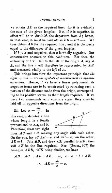
ah
2d. Let x — — .In ^
Therefore, draw two right
lines, AC and AE, making any angle with each other.
On the one, lay off AB =c, and AC= a; on the other,
AD =b. Join BD, and draw CE parallel to BD; then
will AE be the line required. For, (Geom., 307) the
triangles ABD, ACE being similar, we have
AB : AC :: AD : AE; or, c : a :: b : AE.
this case, x denotes a line
whose length is a fourth
proportional to e, a, and b.
e
10 ANALYTIC GEOMETRY.
_ , T abc . ab ,
3d. Let x — y- . Putting -j — k, this may be
written ,
ke
x = — .
9
ab
Therefore, construct k — y, as in the preceding case,
and, with the line thus found, apply the same construc
tion to x.
abed k'd . abe keIn like manner, -j-^ = , by putting k' = -j^ = — •
And, in the same way, we may construct any quotient
of the first degree.
II. The Roots of the Pure Quadratic.—Three or
four cases deserve attention :
1st. Let x = Vab. Here we have a line whose length
is the geometric mean of a and b. There are several
constructions, but the following is as elegant as any.
On any right line, lay off AB — a,
and BO = b. Upon AO = a + b, ,--
describe a semicircle. At B erect a / \
perpendicular meeting the curve in ^— ^
B: BB is the line sought. For
(Geom., 325)
BB = \rABxBC = Vab = x.
Strictly speaking, since the radical Vab has a double
sign, there are two lines answering to x, equal in length,
but measured in opposite directions. And for this, in
fact, the construction provides: since there is a semi
circle below, as well as above AC, to which the per
pendicular dropped from B has the same length as BB,
but is drawn in a direction exactly opposite.
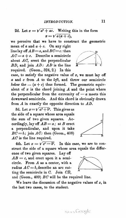
INTRODUCTION. 11
2d. Let x — l/a2 + ae. Writing this in the form
x = Va (a + c),
we perceive that we have to construct the geometric
mean of a and a + c. On any right
line lay offAB= a, andjBC= c : then
A C= a + c. Describe a semicircle
about AC, erect the perpendicular
BD, and join AD: AD is the line
required. (Geom., 324, 2.) In this
case, to satisfy the negative value of x, we must lay off
a and c from A to the left, and throw our semicircle
below the — (a + c) thus formed. The geometric equiv
alent of x is the chord joining A and the point where
the perpendicular from the extremity of — a meets this
downward semicircle. And this chord is obviously drawn
from A in exactly the opposite direction to AD.
3d. Let x=V a2-\-b2. This gives us
the side of a square whose area equals
the sum of two given squares. Ac
cordingly, lay off AB = a; at B erect
a perpendicular, and upon it take
BC= b; join A 0: then (Geom., 408)
AG is the line required.
4th. Let x = VcL — b2. In this case, we are to con
struct the side of a square whose area equals the differ
ence of two given squares. Lay off
AB — c, and erect upon it a semi
circle. From A as a center, with a
radius AC— b, describe an arc cut
ting the semicircle in C. Join CB,
and (Geom., 409) BC will be the required line.
We leave the discussion of the negative values of x, in
the last two cases, to the student.

12 ANALYTIC GEOMETRY.
q. At B erect the
III. Roots of the Complete Quadratic. — Let
us consider the Four Forms separately. (See Alg.,
231.)
1st. The First Form of the complete Quadratic is
x" + %px = q2- 9
Its roots are given in the formula
x = —p ± Vp2 + q*.
To construct these: Lay off AB
perpendicular BC =p. From
C as center, with the radius BO
describe a circle. Join A C, and
produce the line to meet the cir
cle in E: AD and EA are the
required roots. For, by the con-
construction, AC = Vp2 + q2;
and, the first of the above roots having the radical positive,
we must lay it off to the right, from A to C. The neg
ative p must now be laid off to the left, from C to D.
Hence,
AB= —p + Vf + f= x' (1).
In the second of the above roots, the radical is negative.
Both that and p must therefore be measured to the left
from their origin. We begin, then, at E and lay off
EC— — p; continuing in the same direction, OA =
— Vp2 + ql- Whence
EA = —p—Vf + q2 = x" (2).
2d. The Second Form is written
x" — 2px = q-.
* By writing tho absolute term as of the 2d degree, since (Art. 9, 5) the
equation is homogeneous.
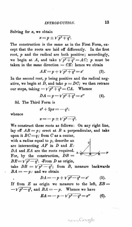
INTROD UCTIOX. 18
Solving for x, we obtain
x=p ± Vp2 + q2.
The construction is the same as in the First Form, ex
cept that the roots are laid off differently. In the first
root, p and the radical are both positive; accordingly,
we begin at A, and take Vp2 + q2 — A C; p must be
taken in the same direction = CE: hence we obtain
AE=p + Vp2 + q2 = x' (3).
In the second root, p being positive and the radical neg
ative, we begin at D, and take p = DC; we then retrace
our steps, taking — Vp2 + q2= CA. Whence
DA =p— Vp2 + q2 = x" (4).
3d. The Third Form is
x2 + 2px = — q2 :
whence
x — —p ± Vp2— q2.
We construct these roots as follows : On any right line,
lay off AB—p; erect at B a perpendicular, and take
upon it BC— q; from C as a center,
with a radius equal to p, describe an
arc intersecting AF in D and E: /j
DA and EA are the roots required.
For, by the construction, DB =
BE=Vp2— q2. -From D as origin,
take DB = Vp2 — q2 ; from B, measure backwards
BA = —p: and we obtain
DA= —p + Vp2— q2 = x> (5).
If from E as origin we measure to the left, EB —
—Vp2— q2, and BA ——p. Whence we have
EA = —p— Vf^q2=x" (6).
14 ANALYTIC GEOMETRY.
4th. The Fourth Form is
x2 — 2px = — q2.
Its roots are
x=p ± V p2— q2.
Using the same general construction as in the Third
Form, we find the linear equivalent of the first of these
by assuming A as origin, taking AB =p to the right,
and, in the same direction, BE=Vp2— q2. Whence,
AE=p + Vf=q2= x' (7).
For the second root, still making A the origin, we have
AB=p, and BD= —Vp2 — q2. Therefore,
AD= p— Vp2— q2 = x" (8).
Remarks.—The constructions just explained furnish
a good example of the clearness and completeness with
which algebraic and geometric properties reflect each
other, when the necessary conventions are established.
Thus,
First: The construction in the First Form reflects the
algebraic property (Alg. 234, Prop. 4th) that the absolute
term of a complete quadratic is equal to the product of
its roots.* For, by the construction, AB — q is tangent
to the circle BBE at B. Hence (Geom., 333) AB2 =
AD X AB. That is, q2 = x'x".
On the other hand, we may see that the algebraic con
dition, q2 — x'x", gives us the geometric property that
the square on the tangent to a circle, from any point with
out the curve, is equal to the rectangle under the segments
*We assume here, as we shall generally throughout the book, that
the absolute term is written in the first member of the equation.
INTRODUCTION. 15
of the corresponding secant. For, multiplying together
equations (1) and (2), we have,
x'x" = ADxEA.
But our condition gives us x'x" — q^\ and, by the con
struction, q2 — AB2. Hence,
AB- = AD X EA.
Now, AB and AE are respectively the tangent and
secant from A to the circle DBE.
Second: If we compare equations (1) and (4), (2) and
(3), we observe that the linear equivalents of x' in (1)
and x" in (4), of x" in (2) and x' in (3), are identical
lengths, measured in opposite directions. In other words,
the positive root of the First Form is the negative root
of the Second, and vice versa. This is as it should be :
for, obviously, the First Form becomes the Second, if
we put — a; for + x.
Third: If, in equations (5), (6), (7), (8), we suppose
p ^> q, the roots are real and unequal. The construc
tion also indicates this. For, so long as the hypotenuse
CD—p is greater than the perpendicular OB= q, it will
intersect AF in two real points.
If we suppose p — q, the roots are real, but equal.
This, too, is involved in the construction. For, when the
radius CD=p becomes equal to CB— q, the circle touches
AF; that is, its two points of section with AF become
coincident in B, and AD = AB = AE.
Fourth: If, in (5), (6), (7), (8), we suppose > p, the
roots become imaginary. With this, again, the construc
tion perfectly agrees. For, if 5 > p, the radius CD is
less than the perpendicular CB, and the circle cuts AF
in imaginary points. The supposition, moreover, re
quires us to construct a right triangle whose hypotenuse
An. Ge. 5.
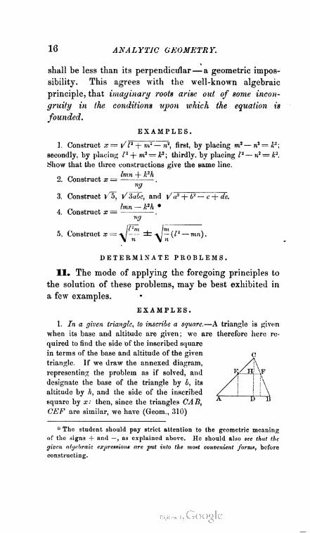
16 ANALYTIC GEOMETRY.
shall be less than its perpendicular— a geometric impos
sibility. This agrees with the well-known algebraic
principle, that imaginary roots arise out of some incon
gruity in the conditions upon which the equation is
founded.
EXAMPLES.
1. Construct x—vli-\-rrit — nl, first, by placing m2 — ns=i2;
secondly, by placing l2 -+- m2 = k2 ; thirdly, by placing I2 — n2 = k2.
Show that the three constructions give the same line.
Imn + k2hA. Construct x = .
ng
3. Construct V 5, V'iabc, and V a' + b2 — c + de.
Imn — k2h *<t. Construct x —
ng
5. Construct x ~ — =t [P — mn) .
DETERMINATE PROBLEMS.
11. The mode of applying the foregoing principles to
the solution of these problems, may be best exhibited in
a few examples.
EXAMPLES.
1. In a given triangle, to inscribe a square.-—A triangle is given
when its base and altitude are given ; we are therefore here re
quired to find the side of the inscribed square
in terms of the base and altitude of the given C
triangle. If we draw the annexed diagram, /\
representing the problem as if solved, and fjZ.H;..\F
designate the base of the triangle by b, its / j j j\
altitude by h, and the side of the inscribed / \ j i \
square by x: then, since the triangles CAB, A u
CEF are similar, we have (Geom., 310)
* The student should pay strict attention to the geometric meaning
of the signs + and — , as explained above. He should also see that the
given algebraic expressions are put into the most convenient forms, before
constructing.

INTRODUCTION. 17
AB : EF : : CD : CH; or, b
bh
: : h : h —x.
That is, the side of the inscribed square is a fourth proportional to
the base, the altitude, and their sum. We therefore construct it as
in Art. 10, I. 2d. Or it may be more conveniently done as follows:
Produce the base of the given tri
angle until BL = h ; through L
draw LM, parallel and equal to
BC; join MA, and from JV, the
point where MA cuts BC, drop a
perpendicular upon AB: then is 5 <5 <3 fe ~~P"
NO the side required. For, letting
fall MP perpendicular to AL, we have, by the similar triangles
MAL, NAB,
AL : AB :: MP : NO; that is, b + h : b :: h : NO.
E
\ \L
NO =bh
b + h ~~ ■
Note.—The student should consider what several positions the
side of the square may assume according as the triangle is acute-
angled, right-angled, or obtuse-angled.
2. In a given triangle, to inscribe a rectangle whose sides are in a
given ratio.—Let x and y represent the two sides, and r their con
stant ratio. Then we shall have
xy (!)•
And, as in the previous example, (the other
symbols remaining the same,) wo obtain the
proportion b : y :: h : h — x.
.-. hy — bh —bx (2).
Eliminating y between (1) and (2),
bhX~ b + rh-
This value we construct in the same manner as the side of the
inscribed square. In fact, as is obvious, the first problem is merely
a particular case of the present one ; for a square is a rectangle, the
ratio between the sides of which is equal to 1. The solution, too,

18 ANALYTIC GEOMETRY.
shows this ; for the value of x in the present example becomes that
obtained in the former, when r = 1.
Produce, then, the base of the given triangle until BL equals
rh ; and complete the
drawing exactly as in
the case of the inscribed
square : the point N, in
which the diagonal AM
cuts the side of the tri
angle, is a vertex of the
required rectangle. Let the student prove this.
3. To draw a common tangent to two given circles.—Here our data
are the radii of the circles, and the distance between their centers.
Let r denote the radius of the circle on the left, and r' that of the
other. Let d = the distance between the centers.
The problem may be otherwise stated : Required a point, from
which, if a tangent be drawn to one of two given circles, it will also
touch the other. From the method of constructing a tangent, (see
Geom., 230,) it follows
that this point is some
where on the line join
ing the centers. Hence,
drawing the diagram as
annexed, it is evident
that our unknown quan
tity is the intercept made
by the tangent on this line ; that is, we let
x = CT.
Now we have (Geom., 333)
MT2=NTXLT; or, MT2 = (x + r) (x — r)
In like manner,
M'T2 = N'TXL'T; or, M'T2= (x — d + r') (x — d -r/) (2).
Expanding, and dividing (1) by (2),
MT2 _ x2 — r2M'T2 ~ (x~df— r/1 ( >■
But, by similar triangles,
MT2 r3
(!)■
MT : M'T :M'T2

INTRODUCTION. 19
Substituting in (3), and reducing,
(r2 - r") x! — 2r*dx + rH a= 0 :
rd
Before constructing this result, let us interpret it. We observe
that our problem involves the solution of a quadratic, and that we
thus obtain a double value for x = CT. The required tangent,
therefore, cuts the line of the centers in two points; that is, there
are two points from which a common tangent to the two circles
may be drawn.9
Let us now consider the two values of x more minutely. We
shall find all the geometric facts of the problem perfectly repre
sented in them.
First take the value numerically the greater, namely,
rdx — z>-
r — r
Since this must be numerically greater than d, and since the
definition of a tangent renders it impossible that the point sought
should fall within either of the circles, the point determined by this
value of x is beyond both. If r > r', x is positive, and the point T
falls to the right of both circles, as in the diagram; if r<r/, x is
negative, and the point then falls to the left of both.
Secondly, the value numerically' the less,
rdx — —rz>-
r r
This is numerically less than d, and, in connection with the defi
nition of the tangent, indicates that the corresponding point lies
between the two circles— a fact with which the sign of x agrees:
for the present value being necessarily positive places the point to
the right of C.
We learn, then, from this analysis, that (1) there are two points
which satisfy the conditions of the problem; that (2) one lies
beyond both circles, and the other between the two; that (3) the
former falls to the right of both circles, or to the left of both, ac
cording as the circle whose center is taken as the origin has a
* Of course, there are four common tangents — two tangents from
any given point to a circle being always possible. But as these exist in
pairs, all the analytic conditions will be exhausted in two. Hence, we
have a quadratic to solve, rather than an equation of the fourth degree.
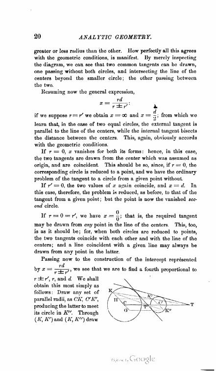
20 ANALYTIC GEOMETRY.
greater or lees radius than the other. How perfectly all this agrees
with the geometric conditions, is manifest. By merely inspecting
the diagram, we can see that two common tangents can be drawn,
one passing without both circles, and intersecting the line of the
centers beyond the smaller circle ; the other passing between
the two.
Resuming now the general expression,
rd
if we suppose r=iy we obtain x — 00 and x — -; from which wo
learn that, in the case of two equal circles, the external tangent is
parallel to the line of the centers, while the internal tangent bisects
the distance between the centers. This, again, obviously accords
with the geometric conditions.
If r — 0, x vanishes for both its forms : hence, in this case,
the two tangents are drawn from the center which was assumed as
origin, and are coincident. This should be so, since, if r = 0, the
corresponding circle is reduced to a point, and we have the ordinary
problem of the tangent to a circle from a given point without.
If r* = 0, the two values of x again coincide, and x = d. In
this case, therefore, the problem is reduced, as before, to that of the
tangent from a given point ; but the point is now the vanished sec
ond circle.
If r — 0 = )y, we have x = ^ ; that is, the required tangent
may be drawn from any point in the line of the centers. This, too,
is as it should be; for, when both circles are reduced to points,
the two tangents coincide with each other and with the line of the
centers; and a lino coincident with a given line may always be
drawn from any point in the latter.
Passing now to the construction of the intercept represented
by x = —gg—/ , we see that we are to find a fourth proportional to
r ± r", r, and d. We shall
obtain this most simply as
follows: Draw any set of
parallel radii, as CK, CK\
producing the latter to meet
its circle in K". Through
{K, K') and (ff, K") draw
INTROD UCTION. 21
right linos: the points T and 2f, in which these intersect the line
of the centers, arc the extremities of the required intercepts. For,
drawing K'H and K"(J parallel to C'T, we have, by similar tri
angles,
: CK :: CC : { £y ; or, rir' : r :: rf : |
V/'ionce,
GT—-^—.\ cr =
cr
ct'
Therefore, draw through T, or J", a tangent to either of the
given circles, and the construction is complete. *
4. To construct a rectangle, given its area and the difference between
its sides.—This problem is of importance, as illustrating the fact
that we are not always to interpret the presence of a quadratic in
our investigations as indicating a double solution of the problem
in hand. On the contrary, a quadratic not unfrequently arises
when but one solution is possible. One of its most important
interpretations in that case, will appear in solving the present
example.
Let (Art. 0, 2) a2 = the given area of the rectangle, and d =
the difference between its sides. Let x = the less side; then will
x + d = the greater.
By the data (Geom., 379) we have
x (x + d) = a2 ; or, x1 + dx = a2.
. • . x — — ^ ± -^a2 -+- ~ = the less side.
/ rf~2-v| "■'"' + -j- = the greater side.x+d = ~±
• This construction, so well adapted for analytic discussion, some
times fails in practice, as the extremity of the outer intercept may not
fall upon the paper. The following elegant construction is practicable in
all cases :
From the center of the larger circle, with a radius equal to the
difference between the given radii, describe a circle, to which draw a
tangent from the center of the smaller circle. A tangent to either given
circle, parallel to this, is tangent to both.

22 ANALYTIC GEOMETRY.
This is a case of the roots of a
quadratic in the First Form. We f
therefore construct x as in Art. 10, j
III, 1. Wc then have, taking the
upper sign in the values of both ^^"^
sides, A
AD = — ^ + a fa1 + ^- = x, the less side ;
x -f- d, the greater.
If we take the lower sign in the values of the two sides, we obtain
—S-^-U+^)1
Comparing with the former values, we see that the present less side
is the negative of the former greater ; and the present greater, the
negative of the former less. Hence, in this case,
— AE = the less side.
— AD = the greater.
It is obvious that the expressions less and greater are here
used in their algebraic sense; for AE is still numerically greater
than AD.
Now, by the construction, (Geom., 333) the rectangle of the
parts gives us
AD X AE= —AE X — AD = AS1 = a1.
Hence, in both cases, the rectangle is positive, . and absolutely the
same. The quadratic, therefore, does not here indicate two solu
tions. It merely signifies that the required rectangle may bo
obtained either by representing its sides by x and x + d, or by
— x and — (x + d). That is, it points not to two rectangles an-
swering the given conditions, but merely to two correlated modes
of expressing the conditions of one and the same rectangle.
We learn, then, that the algebraic discussion of a problem not
only possesses the greatest generality — indicating by the equa
tions to which the problem gives rise every possible solution; but
INTRODUCTION. 23
that, if there are various modes of expressing conditions, which
still lead to the same equation, the equation formed on the basis
of any one of these modes will include all of them in the form of
its roots.
12. From the foregoing examples, we gather the fol
lowing rule for solving Determinate Problems:
Draw a diagram representing the problem as if solved,
inserting any auxiliary lines needed to develop the rela
tions between the known and unknown parts. By means
of the geometric properties which the diagram involves,
form equations between these parts, taking care that they
be independent and equal in number to the unknown
quantities. Construct upon a single figure the roots of
these equations.
A few exercises are added, which the beginner should
carefully perform. In each, let the problem be dis
cussed, as to the number of its solutions, their various
meanings, etc. In the construction, select that method
which is neatest and most convenient.
EXAMPLES.
1. To construct a square of equal area with a given rectangle.
2. In a given triangle, to inscribe a rectangle of a given area.
3. In a given semicircle, to inscribe a square.
4. To draw, parallel to the base of a triangle, a line which shall
divide it into two parts equal in area.
5. Through a given point without a circle to draw a secant
whose internal segment shall be equal to a given line.
6. To describe a circle equal in area to two given ones.
7. To draw, from a given line to a given circle, a tangent of a
given length.
8. To draw, from a given line to a given circle, the tangent of the
least length.
'24 ANALYTIC GEOMETRY.
9. Through two given points, to describe a circle touching a
given right line.
10. In a given circle, to inscribe three equal circles touching
each other externally.
II. INDETERMINATE GEOMETRY.
13. The geometry of Form is called Indeterminate,
because all Forms are conceived to arise out of the rela
tive positions of points ; that is, out of a point's being
so far indeterminate as to be capable of assuming any one
of a series of positions which define a Form : or, from
the algebraic point of view, because the equations which
express the conditions under which a point may vary its
position, are always found to be less in number than the
unknown quantities they contain, and hence, admitting
of an infinite number of values for these, are indeter
minate. 5
14. It is in this second main division of the subject,
that we come upon the proper province of Analytic
Geometry. In fact, as the student has doubtless already
noticed, the method of Determinate Geometry, is rather
that of ordinary geometry than of algebra : the reason
ing is based mainly on the diagram, and the only use
of the algebraic symbol is to abbreviate the terms of
ordinary language. But, in the geometry of Form, as
we shall soon discover, the method is really analytic:
the reasoning is strictly algebraic, while the symbol
has assumed a meaning and power entirely new. In
the articles immediately following, we will endeavor,
first, to show and establish the fundamental principle of
this Geometry of Form, or of Analytic Geometry strictly
so called; secondly, to explain in outline its method and
*Alg., 168.
INTROD UCTION. 25
the reasons for calling it analytic; and thirdly, to un
fold its several subdivisions, especially those discussed
in the body of the present work.
I. DEVELOPMENT OF THE FUNDAMENTAL PRINCIPLE.
15. The principle upon which the whole method of
Indeterminate Geometry is founded is this: The alge
braic symbol of geometric form is the Equation.
IG. The figure of any magnitude is obviously deter
mined by that of its boundaries. Hence, all Forms are
either surfaces or lines. If, then, we can show that an
equation, geometrically interpreted, represents either
some line, or else some surface, the fundamental prin
ciple will be established.
17. There is, of course, no necessary connection be
tween the symbols of algebra and the conceptions of
geometry : the former are merely conventional marks,
denoting magnitudes and operations; while the latter are
forms, which can be imagined and pictured, and which
are necessarily the same to every mind.
18. The truth of the proposition in Art. 15 is ac
cordingly not necessary, but must depend upon certain
arbitrary assumptions. In other words, if the symbols
of algebra are to be applied to represent lines and
surfaces— if symbols of magnitude are to be converted
into symbols of form—we must introduce some conven
tion as to their meaning in the new connection. This
convention, summarily stated, consists in making the
algebraic symbols of magnitude denote the distances, linear
or angular, of a point from certain assumed limits. One
form of it, the most important and characteristic, we will
now illustrate, confining ourselves, for the sake of sim
plicity, to points in a given plane.
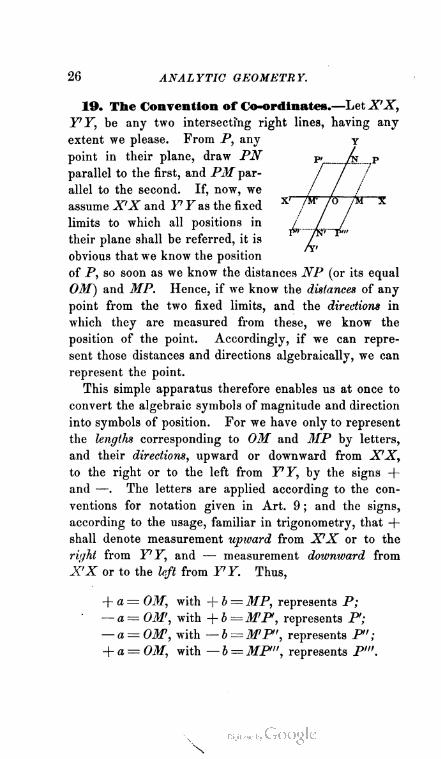
2(3 ANALYTIC GEOMETRY.
19. The Convention of Co-ordinates.—Let X'X,
FF, be any two intersecting right lines, having any
limits to which all positions in / / /
their plane shall be referred, it is /
obvious that we know the position
of P, so soon as we know the distances NP (or its equal
OM) and MP. Hence, if we know the distances of any
point from the two fixed limits, and the directions in
which they are measured from these, we know the
position of the point. Accordingly, if we can repre
sent those distances and directions algebraically, we can
represent the point.
This simple apparatus therefore enables us at once to
convert the algebraic symbols of magnitude and direction
into symbols of position. For we have only to represent
the lengths corresponding to OM and MP by letters,
and their directions, upward or downward from X'X,
to the right or to the left from F7, by the signs +
and —. The letters are applied according to the con
ventions for notation given in Art. 9 ; and the signs,
according to the usage, familiar in trigonometry, that +
shall denote measurement upward from X'X or to the
right from FF, and — measurement downward from
X'X or to the left from FF. Thus,
+ a = OM, with + b =MP, represents P;
■ —a=- OM', with + b =MP, represents P';
— a = OM, with — b = MP', represents P" ;
+ a=OM, with —b=MP", represents P'".
extent we please. From P, any
point in their plane, draw PN
parallel to the first, and PM par
allel to the second. If, now, we
assume X'X and I77 Fas the fixed
Y
s
INTROD UCTION.■27
The lines X'X, Y'Y are called axes; their intersec
tion 0 is called the origin; 031, MP, etc., are called
co-ordinates.
If, now, instead of the particular lines 031, 3IP, etc.,
we take x and y as general symbols for the co-ordinates
of a point, and denote by a and b the values they as
sume for any particular point, we obtain the algebraic
expression for a determinate point in a given plane,
namely,
x = a I
y = b) :
in which a and b may have any value from 0 to go, and
be either positive or negative.
As already hinted, the foregoing is only one form of the
convention upon which rests the whole structure of the
geometry of Form. Several others are used, differing
from the present in the nature of the assumed limits
and of the means by which the point is referred to
them : in some, as in the present one, the co-ordinates
are linear; in others, one of them is angular. The
present form, moreover, applies only to points in a given
plane; forms suitable for representing a point any
where in space, are obtained by assuming for Fixed
Limits planes instead of lines. But whether the forms
of the convention apply to points in space or to points
in a given plane, and however they may differ in their
details, they all agree in this: that a point shall be de
termined by referring it to certain Fixed Limits by
means of certain Elements of Reference, called Co
ordinates.
Definition.—The Co-ordinates of a point are its
linear or angular distances from certain assumed limits.

28 ANALYTIC GEOMETRY.
Corollary.—By the Convention of Co-ordinates
we therefore mean, The agreement that the algebraic
symbols of magnitude shall denote the co-ordinates of a
point.
2©. This convention once established, the connection
between an equation and a geometric form will readily
become apparent. The discovery of this connection, in
its universal bearing, and the first exhaustive applica
tion of it to the discussion of curves, was the work of
the French philosopher Descartes. His method was
first published in 1637, in his treatise Be la Geometric
We shall now show that the connection alluded to really
exists ; but must first define certain conceptions on
which it depends.
21. Variables and Constants.—In analytic inves
tigations, the quantities considered are of two classes:
variables and constants.
Definition.—A Variable is a quantity susceptible, in
a given connection, of an infinite number of values.
Definition.—A Constant is a quantity susceptible of
but one value in any given connection.
Remark.—In problems of analysis, constants impose the con
ditions; variables are subject to them. Constants arc represented
by the first letters of the alphabet; variables by the last. At
times, both are designated by such Greek letters as may be con
venient.
22. Functions.—In the investigations belonging to
Indeterminate Geometry, the variables are so connected
by the conditions of the problem in hand, that any
change in the value of one produces a corresponding
change in that of the others.
Definition.—A Function is a variable so connected
with others, that its value, in every phase of its changes,

INTROI) UCTION. 29
is derived from theirs in a uniform manner. Thus, in
y = ax -f- b, y is a function of x ; in z? = mx3 -\- ny2 + I,
z is a function of x and y.
Remark.—Functions are classed, according to the number of
the variables on which they depend, as functions of one variable,
functions of two variables, etc.
23. With these definitions in view, we may state our
Fundamental Principle with greater exactness, thus :
Every equation between variables that denote the co-ordi
nates of a point, represents, in general, a geometric form.
The proof of this now follows.
24. Equations between Co-ordinates: their
Geometric Meaning.—Every equation is the expres
sion of a constant relation between the variables which
enter it. Further, if we solve any equation for one
of its variables in terms of the others, it becomes ap
parent that such variable is a function of the rest.
Accordingly, by varying either, we may cause all of
them to vary together, by differences as great or as
small as we please ; but, so long as the constants that
express the manner in which each is derived from the
others remain unchanged, all the changes must comply
with one uniform law. That is, whatever be the absolute
value of either variable, its relative value, as compared
with the others, is always the same. If either changes
by infinitely small differences, the others must change
by corresponding infinitesimals.
If, then, we assume that the variables in an equation
denote co-ordinates, the equation itself must represent a
number of points, as many as wc please, all of which
have co-ordinates of the same relative values. Now,
since these co-ordinates vary by differences as small
as we please, the equation really represents an infinite

30 ANALYTIC GEOMETRY.
number of points, lying infinitely near to each other,
and thus forming a continuous series. This continuous
series of positions, moreover, has a definable form, of
the same nature in all its parts; since, from the
definition of an equation, every point in the infinite
succession must comply with a law of position, the same
for all: — a law expressed by the constants in the equa
tion, which subject the variable co-ordinates to an inflex
ible relation in value. Every equation between variables
that denote co-ordinates must therefore, in general,
represent a geometric form.
Remark.—It will represent a line or a surface, according as
the co-ordinates are taken in a plane or in space.
25. A few illustrations will render the principle just
proved still more apparent. For the sake of variety, we
will take these from the converse point of view, from
which it will appear that every attempt to state a law of
form in algebraic symbols results in an equation between
co-ordinates. To simplify, let us confine ourselves to
rectilinear co-ordinates in a given plane, and (since the
axes of reference may be any two intersecting right
lines) suppose X'X, IT to intersect at right angles:
the co-ordinates OM, MP will then be at right angles
to each other.
First: Let it be required to
represent in algebraic symbols
a right line parallel to the axis
Y'Y. The law of this form
plainly permits the variable
point P of the line to be at any
distance above or below X'X,
but restricts it to being at a
constant distance from Y'Y: a condition imposed by
1
P
X' u M X
Y'
P
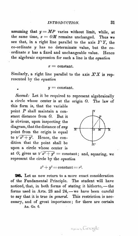
INTROD UCTION. 31
assuming that y = MP varies without limit, while, at
the same time, x = OM remains unchanged. Thus we
see that, in a right line parallel to the axis Y'Y, the
co-ordinate y has no determinate value, but the co
ordinate x has a fixed and unchangeable value. Hence
the algebraic expression for such a line is the equation
x = constant.
Similarly, a right line parallel to the axis X'X is rep
resented by the equation
m V — constant.
Second: Let it be required to represent algebraically
a circle wThose center is at the origin 0. The law of
this form is, that the variable
point P shall maintain a con
stant distance from 0. But it
is obvious, upon inspecting the
diagram, that the distance of any
point from the origin is equal
to V x2 + y2. Hence, the con
dition that the point shall be
upon a circle whose center is
at 0, gives us Vx2 -f y2 = constant ; and, squaring, we
represent the circle by the equation
x2 + y2 = constant = r2.
26. Let us now return to a more exact consideration
of the Fundamental Principle. The student will have
noticed, that, in both forms of stating it hitherto,— the
forms used in Arts. 23 and 24,—we have been careful
to say that it is true in general. This restriction is nec
essary, and of great importance ; for there are certain
An. Ge. 6.

32 ANALYTIC GEOMETRY.
equations which no real values of the variables will sat
isfy: and such, of course, can denote only imaginary, or
impossible, forms. Others can only be satisfied by in
finite values of the variables, and consequently denote a
series of points situated at infinity : a conception as im
possible, geometrically, as that corresponding to the
previous class of equations. Others, again, can be sat
isfied by only one set of real values for the variables,
and therefore represent a single point ; while others,
which can be satisfied by a fixed, finite number of
values, but by no others, represent a finite number of
separate points. Others, still, are satisfied by distinct
sets of values, each set being capable of an infinite
number of values within itself, and having a distinct
relation among the variables which belong to it ; and
such equations represent a group of distinct, though
related forms.
All this makes it clear that, to hold universally, our
Fundamental Principle must be stated in more abstract
terms. We should be obliged to say, merely, that every
equation between co-ordinates represents some conception
relating to form or position, were it not that the happy
expedient of a technical term saves us from this cum
brous circumlocution. It being established that every
equation between co-ordinates has some equivalent in the
province of geometry, it only remains to assign a name
to that equivalent— a name generic enough to include
not only surfaces and lines, but all the exceptional
cases, real, imaginary, or at infinity, that have been
mentioned above.
ST. IiOci.—To include all the cases that may arise
under the conception that an equation has geometric
meaning, the term locus is used.

INTRODUCTION. 33
Definition.—A Locus is the series of positions, real or
imaginary, to which a point is restricted by given con
ditions of form.
Corollary.—Since the locus is the geometric equiva
lent of the equation, we may state the Fundamental
Principle of Indeterminate Geometry universally as fol
lows: Every equation between variables which denote the
co-ordinates of a point, represents a locus.
28. The locus being the fundamental conception of
purely analytic geometry, it is of the utmost importance
that correct views of it be secured at the outset. The
beginner is liable to conceive of it loosely, or else too
narrowly. To guard against these errors, let us illus
trate what has been said or implied above somewhat
more at length.
I. Classification.—Loci are either Geometric or
merely Analytic: the former, when they can be repre
sented in a diagram ; the latter, when they can not.
Geometric Loci include real surfaces, lines, points, and
related groups of either.
Merely Analytic Loci include imaginary loci and
loci at infinity, and loci to be explained hereafter under
the conception of a locus in general. The first have no
existence whatever, except in the equations which sym
bolize them; the last two exist to abstract thought, but
can neither be drawn n_or imagined. The value of con
sidering these merely analytic loci, lies in their important
bearings upon some of the higher problems of the science.
II. Conformity to Law.—It is essential to the con
ception of a locus, that it shall conform to some definite
law. No form that comes within the scope of analytic
geometry can be generated at hazard; no locus is the
least capricious. For it is always the counterpart of an
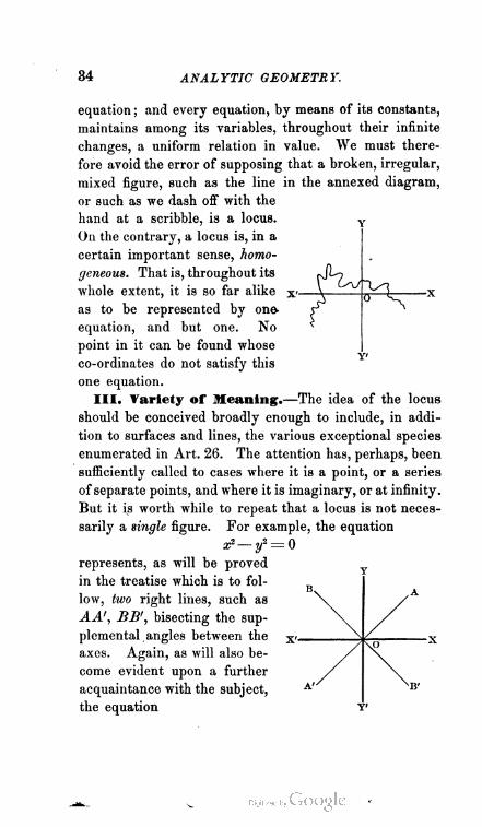
34 ANALYTIC GEOMETRY.
equation ; and every equation, by means of its constants,
maintains among its variables, throughout their infinite
changes, a uniform relation in value. We must there
fore avoid the error of supposing that a broken, irregular,
mixed figure, such as the line in the annexed diagram,
or such as we dash off with the
hand at a scribble, is a locus.
On the contrary, a locus is, in a
certain important sense, homo
geneous. That is, throughout its
whole extent, it is so far alike
as to be represented by one-
equation, and but one. No
point in it can be found whose
co-ordinates do not satisfy this
one equation.
III. Variety of Meaning.—The idea of the locus
should be conceived broadly enough to include, in addi
tion to surfaces and lines, the various exceptional species
enumerated in Art. 26. The attention has, perhaps, been
sufficiently called to cases where it is a point, or a series
of separate points, and where it is imaginary, or at infinity.
But it is worth while to repeat that a locus is not neces
sarily a single figure. For example, the equation
X2— y2 = 0
represents, as will be proved
in the treatise which is to fol
low, two right lines, such as
AA', BB', bisecting the sup
plemental angles between the
axes. Again, as will also be
come evident upon a further
acquaintance with the subject,
the equation
B A
\0
A'' ^B'

INTRODUCTION. 35
represents three circles, such
as 31, M, and M", having
a common center at the
origin.
Examples of this kind
might be greatly multi
plied, but these are perhaps
enough to render the prin
ciple clear, and to fix it in tl
r") (xt + y2—r"*)=0
Y
X
IT'
memory.
H. THE METHOD OUTLINES ; IN WHAT SENSE IT IS
ANALYTIC.
29. The following is a very simple example of the
method by which Analytic Geometry investigates the
properties of figures. The
beginner, of course, must
accept upon authority the
meaning of the equations
employed.
To prove that the tangent
to a circle is perpendicular to
the radius drawn to the point
of contact.—Let the axes be
rectangular, and the center of the circle at the origin.
The equation to the circle is, in that case,
x* + y2 — r2-
The equation to the tangent at any point P, whose co
ordinates are x', y1, is
xfx + y'y = t2 (!)•
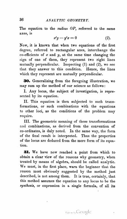
36 ANALYTIC GEOMETRY.
The equation to the radius OP, referred to the same
axes, is
x'y — y'x = 0 (2).
Now, it is known that when two equations of the first
degree, referred to rectangular axes, interchange the
co-efficients of x and y, at the same time changing the
sign of one of them, they represent two right lines
mutually perpendicular. Inspecting (1) and (2), we see
that they answer to this condition. Hence, the lines
which they represent are mutually perpendicular.
30. Generalizing from the foregoing illustration, we
may sum up the method of our science as follows :
I. Any locus, the subject of investigation, is repre
sented by its equation.
II. This equation is then subjected to such trans
formations, or such combinations with the equations
to other loci, as the conditions of the problem may
require.
III. The geometric meaning of these transformations
and combinations, as derived from the convention of
co-ordinates, is duly noted. In the same way, the form
of the final result is interpreted. Thus the properties
of the locus are deduced from the mere form of its equa
tion.
31. We have now reached a point from which to
obtain a clear view of the reasons why geometry, when
treated by means of algebra, should be called analytic.
We must, in the first place, warn the beginner that the
reason most obviously suggested by the method just
described, is not among them. It is true, certainly, that
this method assumes the equation to any locus to be the
synthesis, or expression in a single formula, of all its

INTRODUCTION. 37
properties. It is true that these properties are drawn
out from the equation by a process of real analysis—
namely, by solving or transforming the equation, thus
causing it to give out the several conditions which its
original form unites in one symbol.
But this obvious fact, that we proceed from a com
plex unity to the elements that have vanished into it,
by directly taking apart the unity itself, is not the dis
tinctive reason for calling the Geometry of the Equation
analytic ; for it is a fact which does not distinguish it
from the Geometry of the Diagram. In this last-named
form of the science, the whole scheme of demonstration
consists merely in developing what certain definitions
and axioms imply: that is, the basis of the reasoning—
all that gives it force and validity— is analytic. And,
in fact, the same is true in every department of math
ematics.
32. In short, the term analytic is applied to the
Geometry of the Equation, not so much by way of con
trast, as of emphasis. It should not be taken as imply
ing that the Geometry of the Diagram is wholly synthetic,
and the Geometry of the Equation wholly analytic, each
to the exclusion of the other. Both are analytic, both
synthetic ; and in both, the vital principle of the proofs
is analysis. But to the Geometry of the Equation, the
character of analysis belongs in a special sense, and in a
higher degree; just as that of synthesis belongs, in a
special sense and higher degree, to the Geometry of the
Diagram. It involves, moreover, certain phases of an
alysis, of a higher and more subtle kind than ordinary
geometry attains.
33. Now, this special analytic character, it owes to
its use of the algebraic symbol. The question therefore

38 ANALYTIC GEOMETRY.
naturally arises : How does the use of this symbol bring
with it this special character ? The answer is — In two
ways : first, by giving scope to the analytic tendency
inseparable from algebraic investigation ; secondly, by
introducing the convention of co-ordinates, with its
added elements of analysis. We will illustrate both of
these ways somewhat in detail.
34. Special Analytic Character of the Alge
braic Calculus.—This is due to two facts : the first,
that operations with symbols necessarily thrust into prom
inence the analytic phase of the thinking they imply,
while they obscure the synthetic ; the second, that the
Theory of Equations —the essence of the science of
algebra, and the ground upon which all its investiga
tions are based— is an application of analysis, pecu
liarly complex and subtle. That these are facts, Tvill
best be seen by considering them separately.
I. To exhibit the first, let it be borne in mind that
every demonstration involves both analysis and syn
thesis — analysis, in thinking out the steps connecting
the premise with the conclusion; synthesis, in arrang
ing those steps in their due order, and constructing the
conclusion as their unity. Now, if we use ordinary
language in making this array, clearness can not be
secured without stating these steps one by one ; thus we
seem to begin with parts, and to construct the conclusion
as the whole which they compose.
But if we employ algebraic language, our premise is
written down in a formula, and, at the outset, our atten
tion is fixed upon it as a whole. The formula is the
permanent object of our thought; the operations, the
transformations it undergoes, seem transient and subor
dinate, and their results but dependent phases of its
INTRODUCTION. 3!)
original form. Derived from the formula by a partic
ular series of transformations, while a number of others
are equally possible, the conclusion stands in the mind,
not as a whole but rather as a part. It appears to us
as but one of many elements involved in the original
formula— elements that may be made to show them
selves, if we apply other transformations. Thus the
synthetic phase, though as real here as in using ordi
nary language, is lost to view, and we are only con
scious of the analytic.
II. That the Theory of Equations involves a subtle
and peculiar form of analysis, is obvious, and need not
be enlarged upon. It is sufficient merely to recall its
topics and their accessories, such as the Doctrine of
Co-efficients, the Theory of Roots— their Number,
Form, Situation, and Limits, the Discussion of Series,
and the Binomial Theorem. But it is important to
mention, that, so controlling a part does this Theory
play in the whole science of algebra, and so emphat
ically does it embody a method peculiarly analytic, the
science itself, from its earliest years, has been known by
the name of Analysis. And it was mainly in allusion to
the fact that the Geometry of the Equation brings the
discussion of Form within the scope of this Theory, that
the title analytic was originally applied to it.
35. Elements of Analysis added by the Con
vention of Co-ordinates.—This convention has a
twofold analytic meaning :
I. First, it asserts that the conceptions of Position
and Form are merely relative ones, always implying
certain fixed limits to which they are referred— the
positions of points are their distances from these limits ;
the forms of loci are the relative positions of their con-
An. Qe. 7.

40 ANALYTIC GEOMETRY.
stituent points. This assertion reaches the real essence
of Position and Form, and gives to the science based
upon it an element of analysis not attained in the Ge
ometry of the Diagram.
II. Secondly, in referring the form of every locus to
fixed limits by means of the co-ordinates of every point,
the convention really determines that form by decom
posing it into infinitely small elements. It thus brings
the form under the highest analytic conception known
to mathematics, and prepares for its discussion by the
various branches of the Infinitesimal Calculus.
36. To recapitulate : The Geometry of the Equation
is called Analytic, first, because its use of algebraic
processes puts forward the analytic, and retires the
synthetic phase of every demonstration, thus rendering
us conscious of investigation rather than of proof ;
secondly, because its method consists in applying those
special modes of analysis which mark the Theory of
Equations; thirdly, because its convention of co-ordi
nates penetrates to the real nature of Position and
Form, resolving them into their essential constituents—
Fixed Limits and Distance ; finally and most signifi
cantly, because it resolves all Forms into elements
infinitely small, and thus brings the discussion of loci
within the sphere of the Infinitesimal Calculus— the
highest expression of mathematical analysis.
37. These facts constitute a sufficient reason for pre
ferring to call the science Analytic Geometry, rather
than Algebraic. The former title, more forcibly than
the latter, calls up the characteristics of its method, as
they have been detailed above. Moreover, the term
algebraic is ambiguous; for it is generally used, in con
trast to transcendental, to characterize operations which
INTRODUCTION. 41
involve only addition, subtraction, multiplication, di
vision, or involution and evolution with constant indices.
But Analytic Geometry considers all loci whatsoever,
not only Algebraic but Transcendental, whether the
latter be Exponential, Logarithmic, or Trigonometric.
38. The superiority of the Geometry of the Equation
to that of the Diagram consists partly in its greater
brevity and elegance, but mainly in its greater power
of generalization. For since the equation to any locus
is the complete synthesis of all its properties, our power
of investigating and discovering these is limited only by
our ability to transform the equation and to determine
the form, limits, number, and situation of its roots. And
since every equation denotes some locus, the equations
of the several degrees may be discussed in their most
general forms. Loci may thus be grouped into Orders,
according to the degree of their equations, and proper
ties common to an entire Order may be discovered by
absolute deduction—properties which, if they could be
established at all by ordinary geometry, would in
volve the most tedious processes of comparison and
induction.
III. THE SUBDIVISIONS OF THE SCIENCE.
39. The subdivisions of Indeterminate Geometry refer
to the nature of the loci discussed in each ; and these are
classified, primarily, according to the form of their equa
tions ; secondarily, according to their situation in a plane,
or in space.
40. Hence, the first division of Indeterminate Geom
etry is into Transcendental and Algebraic.
Transcendental Geometry discusses those loci
whose equations involve transcendental functions ; that is,

42 ANALYTIC GEOMETRY.
functions which depend on either a variable exponent, a
logarithm, or one of the expressions sin, cos, tan, etc.
Algebraic Geometry, those whose equations in
volve none but algebraic functions; that is, functions
which imply only the operations of addition, subtraction,
multiplication, division, or involution and evolution with
constant indices.
41. Algebraic loci are classed into Orders, according
to the degree of their equations referred to rectilinear
axes. Thus, the locus whose equation is of the first
degree, is called the locus of the First order; those
whose equations are of the second degree are called loci
of the Second order; and so on.
The loci of the First and Second orders, on account
of their simplicity, symmetry, and limited number, are
considered to form a class by themselves ; and those of
all higher orders are grouped together as a second class.
42. Accordingly, the second division of our subject
is that of Algebraic Geometry into Elementary and
Higher.
Elementary Geometry is the doctrine of loci of
the First and Second orders.
Higher Geometry is the doctrine of loci of higher
orders than the Second.
43. Each of these divisions based upon the form of
the equations considered, falls into the province of
Plane or of Solid Geometry, according as the equa
tions are between plane co-ordinates, or co-ordinates in
space ; that is, according as the system of reference
is iivo intersecting lines, giving rise to two co-ordinates
for every point ; or three intersecting planes, giving rise
to three co-ordinates.
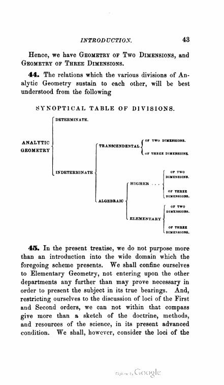
INTROD UCTIOS. 43
Hence, we have Geometry of Two Dimensions, and
Geometry of Three Dimensions.
44. The relations which the various divisions of An
alytic Geometry sustain to each other, will be best
understood from the following
SYNOPTICAL TABLE OF DIVISIONS.
ANALYTIC
GEOMETRY
DETERMINATE.
- OF TWO DIMENSIONS.
INDETERMINATE J
TRANSCENDENTAL |
ALGEBRAIC
OF THIIEE DIMENSIONS.
OF TWO
DIMENSIONS.
OF THREE
DIMENSIONS.
ELEMENTARY
f OF TWO
DIMENSIONS.
OF THREE
DIMENSIONS.
45. In the present treatise, we do not purpose more
than an introduction into the wide domain which the
foregoing scheme presents. We shall confine ourselves
to Elementary Geometry, not entering upon the other
departments any further than may prove necessary in
order to present the subject in its true bearings. And,
restricting ourselves to the discussion of loci of the First
and Second orders, we can not within that compass
give more than a sketch of the doctrine, methods,
and resources of the science, in its present advanced
condition. We shall, however, consider the loci of the

44 ANALYTIC GEOMETRY.
first two orders, both in a plane and in space. Ac
cordingly, our treatise falls naturally into two Books:
the first, upon Plane Co-ordinates; the second, upon
Co-ordinates in Space.
NOTE.
As Greek characters are extensively used in all analytic investi
gations, and as we shall very frequently employ them in the following
pages, we subjoin a list for the benefit of readers unacquainted with
Greek.
A a
r y
A 6
E e
z C
H v
e e
alpha.
beta.
gamma.
delta.
epsilon.
zeta.
eta.
theta.
I i iota.
K k kappa.
A X lambda.
M/i mu.
N v nu.
S f xi.
0 o omicron.
II 7r pi.
Pp
2 a
T T
r v
rho.
sigma.
tau.
upsilon.
phi.
ehi.
psi.
omega.

BOOK FIRST:
PLANE CO-ORDINATES.

PLANE CO-ORDINATES.
PART I.
THE REPRESENTATION OF FORM BY
ANALYTIC SYMBOLS.
46. In applying to plane curves of the First and
Second orders the method sketched in the foregoing
pages, our work will naturally divide itself into two
portions : we shall first have to determine the equations
which represent the several lines to be discussed; and
then deduce from these equations the various properties
of the corresponding lines. Accordingly, our First Book
falls into two parts :
Part I.—On the Representation of Form by An
alytic Symbols.
Part II.—On the Properties of Conics.
47. We say Properties of Conics, because, as will be
shown hereafter, all the lines of the First and Second
orders may be formed by passing a plane through a
right cone on a circular base. By varying the position
of the cutting plane, its sections with the conic surface

48 ANALYTIC GEOMETRY.
will assume the forms of the several lines; and these
may therefore he conveniently grouped under the gen
eral name of Conic Sections, or Conies.
It must be added, however, that this use of the term Conies is
wider than ordinary. For, speaking strictly, we mean by the
Conies the curves of the Second order alone; namely, the Ellipse,
the Hyperbola, and the Parabola; and ordinarily the line of the
First order is not included in the term.
48. We shall therefore proceed to develop the modes
of representing in algebraic language the Right Line,
the Circle, the Ellipse, the Hyperbola, and the Parabola.
And as these modes of representation are all derived
from the conventions adopted for representing a point,
we shall begin by explaining in full the principal forms
of those conventions, which were merely sketched in
the Introduction.
We shall obtain, first, the formulae in ordinary use, or
those which may be said to constitute the Older Geom
etry; and, afterward, those belonging to the Modern
Geometry, based on what is called the Abridged No
tation.
CHAPTER FIRST.
THE OLDER GEOMETRY: BILINEAR AND POLAR
CO-ORDINATES.
Section I.—The Point.
BILINEAR OR CARTESIAN SYSTEM OF CO-ORDINATES.
49. Resuming the topic and diagram of Art. 19,
let us examine the Cartesian* system of co-ordinates
* Cartesian, from Cartesius, the latinized form of Descartes' name.

BILINEAR CO-ORDINATES. 49
more minutely, and develop its elements in complete
detail.
The distances OM, MP being /Y,
known, the position of P is de
termined. These distances are called the bilinear co
ordinates of the point P. They are also termed recti
linear, and sometimes parallel, co-ordinates. They are
frequently cited as the Cartesian co-ordinates of the
The co-ordinate MP, drawn parallel to Y'Y, is called
the ordinate of the point P. The co-ordinate OM,
which the former cuts off from X'X, is called the abscissa
of the point. The abscissa of a point is represented by
the symbol x; its ordinate, by the symbol y.
The two lines X'X and Y'Y are called the axes of
reference, or simply the axes. X'X, on which the ab
scissas are measured, is called the axis of abscissas; or,
more briefly, the axis of x. Y' Y, parallel to which the
ordinates are drawn, is called the axis of ordinates; or,
for brevity, the axis of y.
The point 0, in which the axis of x cuts the axis of y,
is called the origin.
The angle YOX is called the inclination of the axes.
It is designated by the Greek letter to, and may have
any value from 0 to 180°. If to = 90°, the axes and
co-ordinates are said to be rectangular; if to has any
other value, they are said to be oblique.
The two axes, being of infinite length, divide the
P being any point on a given
plane, two right lines X'X and
FY are drawn in that plane,
intersecting each other in 0.
From P, a line PM is drawn
parallel to Y'Y.
point.
50 ANALYTIC GEOMETRY.
whole planar space about 0 into four angles. These
are numbered to the left, beginning at the line OX.
XOY is the first angle; YOX' is the second; X'OY,
the third; and YOX, the fourth.
The signs + and — are used in connection with the
co-ordinates, and are taken to signify measurement in
opposite directions. Positive abscissas are measured to
the right from 0, as OM; negative ones, to the left; as
OM. Positive ordinates are measured upward from XX,
as MP; negative ones, dotvnward ; as MP".
By attributing proper values to the co-ordinates x and
?/, and taking account of their signs, we may represent
any point in either of the four angles. Thus,
x — -j- adenotes a point in the first angle.
" " " second "
" " " third "a I « U i
■=—bi
Z^_l} " " " fourth'
x — — a
y = +t>.
x = -
y
X =
y
Corollary 1.—For any point on the axis of x, we shall
evidently have
y=0,
while x, being susceptible of any value whatever, is in
determinate. Hence, the equation just written is the
equation to the axis of x.
Corollary 2.—For any point on the axis of y, we shall
have
x = 0,
while y is indeterminate. Hence, the equation last writ
ten is the equation to the axis of y.
BILINEAR CO-ORDINATES. 51
Corollary 3.—For the origin, we shall obviously have
x = 0,
y = 0;
and these expressions are therefore ihe symbol of the origin.
Remark 1.—For the sake of brevity, any point
designated by Cartesian co-ordinates is written and
cited as the point x y, the point a b, the point (3, 5), etc.
These expressions are not to be confounded with alge
braic products.
Remark 2.—The symbols x and y are used for co
ordinates of a variable point, and are therefore general in
their signification. But it is often convenient to repre
sent particular, or fixed, points by the variable symbols ;
especially when their positions, though fixed, are arbi
trary. In such cases accents, or else inferiors, are used
with the x and y. Thus a/ y', x" y", xl y„ x2 y.2, all rep
resent points which are to be considered as fixed, but
fixed in positions chosen at pleasure. This distinction
between the point x y as general, and points such as
x1 y', x2 y2 as particidar, should be carefully remembered.
Remark 3.—A point is said to be given by its co
ordinates, when their values and that of the angle co are
known. And when so given, the point may always be
represented in position to the eye. For we have only to
draw a pair of axes with the given inclination, and lay
off by any scale of equal parts we please the given ab
scissa and ordinate. In practice, it is most convenient
to lay off the co-ordinates on the axes, and draw through
the points thus determined, lines parallel to the axes ;
the intersection of the latter will be the point required.
The truth of this will be apparent on inspecting the dia
gram at the head of this article.
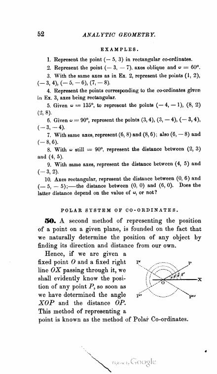
52 ANALYTIC GEOMETRY.
EXAMPLES.
1. Represent the point (— 5, 3) in rectangular co-ordinates.
2. Represent the point (— 3, — 7), axes oblique and u = 00°.
3. With the same axes as in Ex. 2, represent the points (1, 2),
(-3, 4), (-5, -6), (7,-8).
4. Represent the points corresponding to the co-ordinates given
in Ex. 3, axes being rectangular.
5. Given <■> — 135°, to represent the points (— 4, — 1), (8, 2)
(2, 8).
6. Given a = 90°, represent the points (3, 4), (3, — 4), (— 3, 4),
(-3,-4).
7. With same axes, represent (6, 8) and (8, 6) ; also (6, — 8) and
(—8,6).
8. With u still = 90°, represent the distance between (2, 3)
and (4, 5).
9. With same axes, represent the distance between (4, 5) and
(-3, 2).
10. Axes rectangular, represent the distance between (0, 6) and
(— 5, — 5) ; the distance between (0, 0) and (6, 0). Does the
latter distance depend on the value of u, or not?
POLAR SYSTEM OF CO-ORDINATES.
50. A second method of representing the position
of a point on a given plane, is founded on the fact that
we naturally determine the position of any object by
finding its direction and distance from our own.
Hence, if we are given a
fixed point O and a fixed right f
line OX passing through it, we
shall evidently know the post- (
tion of any point P, so soon as
we have determined the angle p»
XOP and the distance OP.
This method of representing a
point is known as the method of Polar Co-ordinates.
• o \
POLAR CO-ORDINATES. 53
The fixed point 0 is called the pole; the fixed line OX,
the initial line.
The distance OP is termed the radius vector; the angle
XOP, the vectorial angle. It is customary to represent
the former by the letter p, and the latter by 6. In this
system, accordingly, a point is cited as the point p 0,
the point p' 8', etc.
By attributing proper values to p and 0, we may repre
sent any point whatever in the plane PXO. Thus,
p = OP
0 = XOP
p> — OP
0' =XOP
j- denotes the point P.
p" = OP" \
0" = XOP" i
p.
P".
nm — Q pin -)r — ujr I « " « pin
0"' = XOP" j
The student will observe that all the angles 6, 0', 6",
6"' are estimated from XO toward the left.
Corollary 1.—For the pole, we evidently have
p = 0:
which may therefore be considered as the equation to that
point.
Corollary 2.—For any point on the initial line to the
right of the pole, we have
6 = 2 n ?r *
For any point on the same line to the left of the pole,
we have
0 = (2 » + 1) jr.
* We shall frequently employ the symbol tt = the semi-circumference
to radiu3 1, to denote the angle 180° ; on the principle that angles are
measured by the arcs which subtend them.

54 ANALYTIC GEOMETRY.
In these expressions, n may have any integral value
from 0 upward.
Note—It is customary to measure the angle 8 from XO toward
the left; and the radius vector p, from O in such a direction as to
bound the angle. When any distinctions of sign are admitted in
polar co-ordinates, the directions just named are considered positive;
while an angle measured from OX toward the right, and a radius
vector measured from O in the direction opposite to that which
bounds its angle, are considered negative. Thus, the point P is
commonly denoted by the positive angle 8 = XOP and the positive
vector p — OP ; but it may also be represented by the negative angle
XOP'* = — (~ — 6) and the then negative vector p = OP. And,
again, the same point may be represented by the positive angle
0" = 0 + ir = XOP" and the negative vector p = OP.
The student will not fail to note that the signs + and —, as
applied to a line revolving about a fixed point, have a signification
quite different from that in connection with bilinear co-ordinates.
They discriminate between radii vectores, not necessarily as measured
in opposite directions, but in directions having opposite relations to the
bounding of the vectorial angle. We may therefore define the positive
direction of a radius vector to be that which extends from the pole
along the front of the vectorial angle ; and the negative, to be that ex
tending opposite.
In practice, negative values of p and 8 are excluded from the
ordinary formulas; but the distinction of sign just explained has an
important bearing on the principles of the Modern Geometry. For
this reason, it should be mastered at the outset.
Remark.—To represent any point given in polar co
ordinates, we have only to draw the initial line, and lay
off at any point taken for the pole, an angle equal to
the given angle 6 : then the distance p being measured
from the pole, the required point is obtained.
EXAMPLES.
1. Represent in polar co-ordinates the point (p = 8; 0 = 7r).
2. Represent (p = — 8 ; 8 = 0) and (p = — 8 ; 8 = ir).
3. Represent (p = 15 ; B =--) and (p — 5 ; 8 = ^V
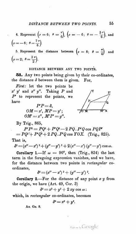
DISTANCE BETWEEN TWO POINTS. 55
4. Represent (p = 6 ; f = ^ = — 6 ; 0 = — and
5. Represent the distance between (p = 8 ; 8 =
DISTANCE BETWEEN ANY TWO POINTS.
51. Any two points being given by their co-ordinates,
the distance 3 between them is given. For,
First: let the two points be
x1 y' and x" y". Taking P and
P to represent the points, we
have
PP= 3,
OM=x', MP= y';
OM = x", MP = y".
By Trig., 865,
P'P> = PQ2 + PQ2— 2PQ.P'Q cos PQF
= PQ2*+ P Q2 + 2 PQ.P'Q cos YOX. (Trig., 825).
That is,
<J2 = (x" — x>) 2 + (y»—y')2Jr2 (x»— x1) (y"—y>) cos to.
Corollary 1.—If a> = 90°, then (Trig., 834) the last
term in the foregoing expression vanishes, and we have,
for the distance between two points in rectangular co
ordinates,
Corollary 2.—For the distance of any point x y from
the origin, we have (Art. 49, Cor. 3)
(J2 = x2 + y2 + 2 xy cos co :
which, in rectangular co-ordinates, becomes
d2=x2 + y2.
An. Ge. 8.
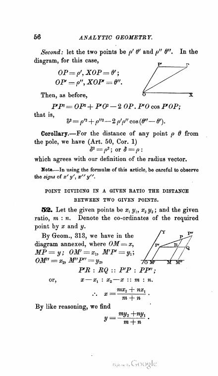
56 ANALYTIC GEOMETRY.
Second : let the two points be p' and p" 0". In the
diagram, for this case,
OP= [>', X0P=6';
OP' = p", XOP = 0".
Then, as before,
PP2 = OP» + PO2— 2 OP. P'O cos POP;
that is,
V = pn + p»i—2 (>'(>" cos (/?"— 0')-
Corollary.—For the distance of any point p 0 from
the pole, we have (Art. 50, Cor. 1)
£2 _ ^2 . or § _ p .
which agrees with our definition of the radius vector.
Note—In using the formulas of this article, be careful to observe
the signs of x' y', x" y".
POINT DIVIDING IN A GIVEN RATIO THE DISTANCE
BETWEEN TWO GIVEN POINTS.
52. Let the given points be xt ylf x2y2; and the given
ratio, to : n. Denote the co-ordinates of the required
point by x and y.
By Geom., 318, we have in the
diagram annexed, where OM=x, /pi
MP = y; OM' = xv MP = yl; / /
OM' = x2,M"P" = y2, -yUr
PR : BQ :: P'P : PP" ;
or, x — xY : x2 —x :: to : n.
mx2 + nx,' $ — 1 ,
to + n
By like reasoning, we find
my2 +ny1
" m-\-n

DISTANCE DIVIDED IN GIVEN RATIO. 57
If the distance between two points xl y„ x2 y2 were
cut externally in the given ratio, we should have
x — xl : x — x2 : : m : n.
mxo — nx,
.-. x — — ;m— n
and, similarly,
myf2 — nyx
" m— n
And this we should expect : for, if the point P fell
beyond P", the segment PP" would be measured in the
direction opposite to P'P, and n would have the negative
sign.
53. As the student may have surmised from what he
has already noticed, formulas referred to rectangular axes
are generally simpler than those referred to oblique. For
this reason, it is preferable to use rectangular axes when
ever it is practicable. Hereafter, then, the attention
should be fixed chiefly upon those formulas which corre
spond to rectangular axes. In some cases, formulas are
true for any value of a). Such are those deduced in the
last article. In the examples given hereafter, the axes
are supposed to be rectangular, unless the contrary is men
tioned.
EXAMPLES.
1. Draw the triangle whose vertices are (2, 5), (— 4, 1),
(-2,-6).
2. Find the lengths of the three sides of the same triangle.
3. Express algebraically the condition that x y is equidistant
from (2, 3) and (4, 5). Ans. x + y = 7.
4. Find the distance between (— 3, 0) and (2, — 5).
5. Determine the co-ordinates of the point equidistant from the
three points (1, 2), (0, 0), and (—5, — 6).

58 ANALYTIC GEOMETRY.
6. Solve Ex. 2, supposing <j successively Z and -g ■
7. Find the co-ordinates of the point bisecting the distance
between Xi j/i and x2 yi
8. The point x y is midway between (3, 4) and (— 5, — 8):
find its distance from the origin.
9. x y divides externally the distance between (2, — 8) and
(— 5, — 3) in the ratio 6 : 7. What is its distance from the point
midway between (3, 4) and (6, 8)?
10. Given the points (p = 5 ; 0 = 30°) and (p = 6 ; 0 = 225°) to
find the distance between them, and the polar co-ordinates of its
middle point.
TRANSFORMATION OF CO-ORDINATES.
54. A point being given by its co-ordinates, we can
at pleasure change either the axes or the system to
which they refer it. The process is called Transforma
tion of Co-ordinates.
The position of the point is of course not affected by
such a change. Its co-ordinates merely assume new values
corresponding to the new axes or new system.
The transformation is effected by substituting for the
given co-ordinates their values in terms of the elements be
longing to the new limits. General formulae for these substi
tutions are easily obtained. In investigating them, it is
convenient to consider the subject in four cases; namely,
I. To change the Origin, the direction of the axes
remaining the same.
II. To change the Inclination of the Axes, the origin
remaining the same.
III. To change System—from Bilinears to Polars, and
conversely.
IV. To change the Origin, at the same time trans
forming by II or III.

TRANSFORMATION OF CO-ORDINATES. 59
55. Case First: To transform to parallel axes through
a new origin.
Let x and y be the co-ordinates of the point for the
primitive axes ; and X and Y its co-ordinates for the
proposed parallel axes. Let
m, n be the co-ordinates of
the new origin. Then, if OY,
OX represent the primitive
axes, and O'Y', O'X' the
new : we shall have x = OM,
y = MP; X=0'M', Y=
MP; and m = 0S, n= SO'.
Now, from the diagram,
OM=OS + O'M' and MP= SO' + MP;
that is, x —m + X,
y = n+Y:
which are the required formulae of transformation.
56. Case Second : To transform to new axes through
the primitive origin, the inclination being changed.
Let to represent the inclination of the primitive axes.
Let a = the angle made by the new axis of x with the
primitive ; and /? = that made by the new axis of y.
Drawing the annexed dia
gram, we have x — OM, y
= MP; X = OM', Y =
MP; a = X'0X = M'OE,
and p = Y'OX = PM'S.
Then, letting fall PQ and
M'R perpendicular to OX,
and M'S perpendicular to
PQ, we obtain (Trig., 858)
MP sin PMQ =QP = RM + SP.
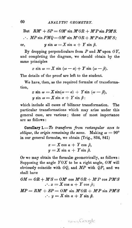
60 ANALYTIC GEOMETRY.
But RM' + SP= OM' sin M'OR + M'P sin PMS.
. • . MP sin PMQ= OM' sin WOR + M'Psin iW/S1;
or, y sin at =X sin « + Y sin /?.
By dropping perpendiculars from P and M' upon 0]T,
and completing the diagram, we should obtain by the
same principles
x sin at = X sin {co — a) + Y sin (at — ft).
The details of the proof are left to the student.
We have, then, as the required formulas of transforma
tion,
x sin co =-3Tsin(fti — «) + !Fsin (co — /5),
y sin at — X sin « + P" sin /9 :
which include all cases of bilinear transformation. The
particular transformations which may arise under this
general case, are various ; those of most importance
are as follows :
Corollary 1.—To transform from rectangular axes to
oblique, the origin remaining the same. Making co — 90°
in our general formulae, we obtain (Trig., 834, 841)
x = X cos a + Y cos /9,
y = X sin a -j- !Fsin {3.
Or we may obtain the formulae geometrically, as follows :
Supposing the angle YOX to be a right angle, OM will
obviously coincide with OQ, and MP with QP, and we
shall have
OM=OR + M'S = OM cos M'OR + M'P cos PM'S
.' . x — X cos a + Y cos /3 ;
iffP = iZM' + SP= OM' sin MOR + M'P sin PlfS
. • . y = X sin a + !F sin
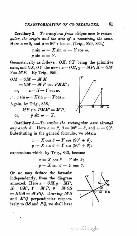
TRANSFORMATION OF CO-ORDINATES. 61
Corollary 2—To transform from oblique axes to rectan
gular, the origin and the axis of x remaining the same.
Here a = 0, and 0 = 90° : hence, (Trig., 829, 834,)
x sin co = X sin «» — Y cos «,
2/ sin co — Y.
Geometrically as follows : OX, OY being the primitive
axes, and OX, 0F the new : x= OM, y = MP;X= OM>
Y=MP. By Trig., 859,
OM= OM'— M'M
= OM>—MP cot PMM ;
or, x—X— Ycot co.
.-. resin w=Xsin W— Ycosco.
Again, by Trig., 858,
MP sin PMM' =MP;
or, y sin co = Y.
Corollary 3.—To revolve the rectangular axes through
any angle 0. Here a = 0, /? = 90° + d, and co — 90°.
Substituting in the general formulae, we obtain
x = Xcos 0 + Y cos (90° + ff),
y = X sin 0 + Y sin (90° + 0) :
expressions which, by Trig., 843, become
x =X cos 0 — Y sin 0 ;
y =X sin 0 + J" cos 0.
Or we may deduce the formulae
independently, from the diagram
annexed. Here x - OM,y=MP;
X=OM, Y= M'P; 0 = M'OS
=ROM=M'PQ. Drawing M'S
and M'Q perpendicular respect
ively to OS and PQ, we shall have
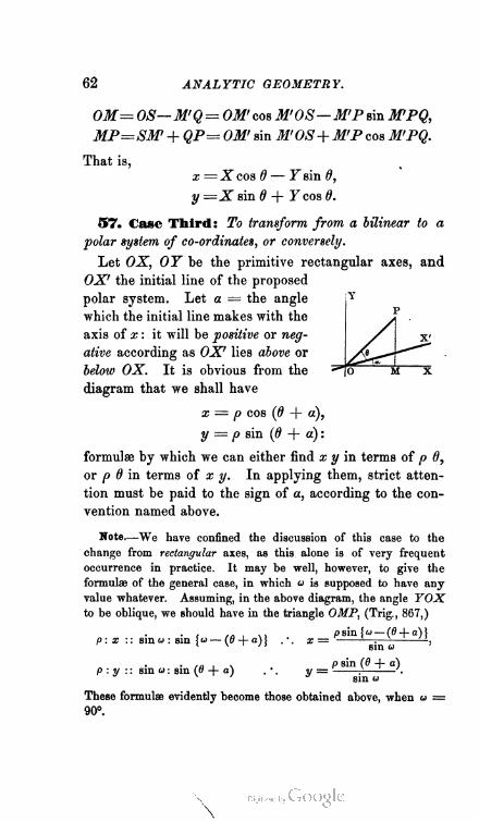
62 ANALYTIC GEOMETRY.
0M= OS—M'Q = OM' cos M'OS—M'P sin M>PQ,
MP=SM' + QP= OM sin M'OS+M'P cos M'PQ.
That is,
x =X cos 0 — Y sin 0 ,
2/=Xsin0 + Fcostf.
57. Case Third: To transform from a bilinear to a
polar system of co-ordinates, or conversely.
Let OX, OF be the primitive rectangular axes, and
OX' the initial line of the proposed
polar system. Let a = the angle
which the initial line makes with the
axis of x : it will be positive or neg
ative according as OX' lies above or
below OX. It is obvious from the
diagram that we shall have
x = p cos (0 + a),
y = p sin (0 + a) :
formulae by which we can either find x y in terms of p 0,
or p 0 in terms of x y. In applying them, strict atten
tion must be paid to the sign of a, according to the con
vention named above.
Note—We have confined the discussion of this case to the
change from rectangular axes, as this alone is of very frequent
occurrence in practice. It may be well, however, to give the
formulas of the general case, in which a is supposed to have any
value whatever. Assuming, in the above diagram, the angle YOX
to be oblique, we should have in the triangle OMP, (Trig., 867,)
• ( fa i \) Psm — (e + a)}p : x : : sin a : sin ia — (0 + a) J .-. x — • ' ■ v——1 x ' ' sin a
■ ,a i \ P sin (8 + a)p : v : : sin a : sin (8 + a) . • . y = H ■
* v ' * sinu
These formulae evidently become those obtained above, when a =
90°.

TRANSFORMATION OF CO-ORDINATES. 68
Corollary.—If the axis of x is taken as the initial line,
a — 0 ; and we have
x = p cos 0,
y — p sin 0 :
a set of formulae in very extensive use.
58. Case Fourth: To combine a change of origin
with any other transformation.
To effect this, we first apply the formulae of Art. 55,
and thus pass to the new origin with a system of axes
parallel to the primitive. That is, in effect, we remove
the original system to the new position which the proposed
origin requires. The formulae for the special transforma
tion in hand are then applied, and the whole change is
accomplished.
From the nature of the formula? in Art. 55, it is obvious
that the present case is solved analytically by merely
adding to the expressions for x and y, the co-ordinates
m and n of the new origin. Thus, in general, by Art. 56,
, X sin (to — a) + Y sin (to — S)x = m H t1 ; J — ,
sin — to ■ f
, X sin a + Y sin 8
y — n -\ :y sin to '
To pass from bilinears to polars when the pole is a dif
ferent point from the origin, we have
x — m + p cos (d + a),
y = n + p sin (6 + «)■
59. It should be observed that in applying these
various formulae, great care is to be exercised in respect
to the signs of the constants involved. And in the ex
amples which follow, where given points are to be trans
formed, the same care should be taken with respect to all
An. Ge. 9.

64 ANALYTIC GEOMETRY.
the known co-ordinates. It is recommended that the
student reduce every problem to drawing, at least in the
earlier stages of his studies. In no other way will he
readily acquire the habit of bringing every analytic
process to the test of geometric interpretation.
EXAMPLES.
1. Given the point (5, 6) : what are its co-ordinates for parallel
axes through the origin (2, 3)?
2. Transform (— 3, 0) to parallel axes through (— 4, — 5);—
to parallel axes through (5, —3); — through (—3, 5); — through
(-3,0).
3. Given in rectangular co-ordinates the points (1, 1), (— 1, 1),
(2, — 1), and (— 3, — 3). find their polar co-ordinates, the origin
being the pole, and the axis of x the initial line.
4. Transform the points in Ex. 3, supposing the pole to be at
( — 4, 5), and the initial line to make with the axis of x an angle
„ = _ 30°.
5. Solve Ex. 4, on the supposition that a = 45°.
6. Find the rectangular co-ordinates of (p = 3; 8 = 60°) and
(/> = — 3 ; 6 = — 60°), the origin and axis of x coinciding respect
ively with the pole and the initial line. Find the same, supposing
the origin at (— 2, — 1), and the angle a = 30°.
7. The co-ordinates of a point for a set of axes in which u =
60°, satisfy the equation 'Ax + 4y — 8=0: what will the equation
become when transformed to i/ = 45° a = 15°? What, when in
addition the origin is moved to (—3, 2)?
8. Transform x1 + y1 = r2 to parallel axes through (— a, — b).
9. It is evident that when we change from one set of rectangular
axes to another having the same origin, x2 + y% must be equal to
a/2 + y'2, since both express the square of the distance of the point
from the origin. Verify this by squaring the expressions for x and
y given in Art 56, Cor. 3, and adding the results.
10. Transform to rectangular co-ordinates the following equations
in polar ; origin same as pole, and axis of x as initial line :
P2sin20 = 2c2; p*cos £0= c*; p2 = c2 cos 2 0.

INTERPRETA TION IN GENERA L. 65
GENERAL PRINCIPLES OF INTERPRETATION.
60. In an important sense, the whole science of
Analytic Geometry may be said to consist in knowing
how to translate algebraic symbols into geometric facts.
Supposing that we have solved any geometric problem
by analytic methods, our result must be some algebraic
expression. Hence, in the end the question is, How
shall we interpret that expression into the geometric
property which we are seeking ?
The principles governing such an interpretation are to
be mastered in their fullness, only through an exhaustive
study of the whole field of Analytic Geometry.' But
there are a few of them, which, lying at the root of all
the others, are of universal application, and must be de
termined at the outset. In the following articles, we
will state and establish them. The student may notice
that the illustrations and, in some cases, the phraseology
refer to Cartesian co-ordinates ; but this does not affect
the generality of the principles, since we can convert any
geometric expression into one relating to the Cartesian
system by transformation of co-ordinates.
61. A single equation between plane co-ordinates repre
sents a plane locus.
This theorem follows directly from the corollary of
Art. 27. It may be well, however, to add here some
illustrations of the principle.
It is plain that if we have any equation between two
variables, as ^
ax? -f bx2y + cxy2 + dy* +/-= 0,
we may assign to x any value we please, and obtain a
corresponding value for y. The unknown quantities in
such an equation are therefore not determinate. On the
contrary, there is a series of values, infinite in number,

G6 ANALYTIC GEOMETRY.
any of which will satisfy the equation. Taking these
values as denoting the co-ordinates of a point, the equa
tion must represent an infinite number of points. . But,
though infinite in number, these points can not be taken
at random; for the equation can not be satisfied by
values arbitrary for y as well as x, but only by such
values of y as its own conditions require in answer to
the assigned values of x. Hence, the infinite series
of points which the equation represents, conforms in all
its members to the same law of position : a law ex
pressed in the uniform relation which the equation
establishes between the values of its variables. Such a
series of points must constitute a line.
To illustrate by a diagram,
we may suppose that in a
given equation between two va
riables, x has the value Om.
Corresponding to this there will
be, let us say, three values of y,
represented by mp, mq, mr. We
thus determine three points, p,
q, r. Again, supposing x = Om', we determine three
other points, p', q', r'. And again, making x = Om",
we obtain the points p", q", r". We may continue this
process as long as we please, and determine any number
of points, by assigning successive values to x. By taking
these sufficiently near each other, and drawing a line
through the points thus found, we may determine the
figure of the locus which the equation represents.
Remark.—We must here carefully recall the proposition, stated
in the Introduction, that to render the principle of this article uni
versally true we must take into account imaginary loci, loci at
infinity, and cases where a locus degenerates into disconnected points
or a single point. For example, the equation
x> + y2 + 1 = 0
INTERPRETATION IN GENERAL. 67
can not be satisfied by any real values of x and y : consequently, in
order to bring it within the terms of our principle, we must say that
it denotes an imaginary locus. It should be borne in mind that
this amounts to saying that it has no geometric locus.
Again, the equation
Ox + Oy + c = 0
can be satisfied by none but infinite values of x and y. All the
points on its locus are therefore at an infinite distance from the
origin, and it can be brought within the terms of our principle only
by saying that it denotes a locus at infinity. This, too, is only another
way of saying that it has no geometric locus.
Again, the equation
Or-a)*+ys = 0
obviously can not be satisfied unless we have, at the same time,
{x — a)2= 0 and f — 0;
that is, it admits of no values except
x = a and y = 0.
Accordingly, if we would bring it within our principle, we must say
that it denotes a locus which has degenerated into a point situated on
the axis of x, at a distance a from the origin. We shall learn here
after that this point is an infinitely small circle, having (a, 0) for
its center.
62. Any two simultaneous equations between plane co
ordinates represent determinate points in a given plane.
For, given two equations between two variables, we
can determine the values of x and y by elimination.
Moreover, the points which such a pair of simultaneous
equations determines, are the points of intersection common
to the two lines which the equations respectively repre
sent. For it is obvious that the values of x and y found
by elimination, must satisfy both of the equations ; hence,
the points which these values represent must lie on both
of the lines represented by them : that is, they are the
points common to those lines.
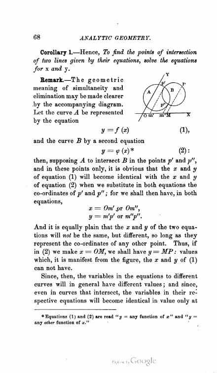
68 ANALYTIC GEOMETRY.
Corollary 1.—Hence, To find the points of intersection
of two lines given by their equations, solve the equations
for x and y.
Remark.—The geometric
meaning of simultaneity and
elimination may be made clearer
by the accompanying diagram.
Let the curve A be represented
by the equation
y=/(«) (i),
and the curve B by a second equation
* = ?(*)* (2):
then, supposing A to intersect B in the points p' and p",
and in these points only, it is obvious that the x and y
of equation (1) will become identical with the x and y
of equation (2) when we substitute in both equations the
co-ordinates of p' and p" ; for we shall then have, in both
equations,
x = Om' ,pr Om",
y = m'p' or m"p".
And it is equally plain that the x and y of the two equa
tions will not be the same, but different, so long as they
represent the co-ordinates of any other point. Thus, if
in (2) we make x — OM, we shall have y = MP : values
which, it is manifest from the figure, the x and y of (1)
can not have.
Since, then, the variables in the equations to different
curves will in general have different values ; and since,
even in curves that intersect, the variables in their re
spective equations will become identical in value only at
* Equations (1) and (2) are read "y = any function of x" and "y —
any other function of x."
INTERPRETATION IN GENERAL. 69
the points of intersection ; we learn the important principle,
that to suppose two geometric equations simultaneous is
to suppose that their loci intersect. In short, simultaneity
means intersection ; and elimination determines the intersect
ing points.
Corollary 2.—Two equations, of the m"' and n"1 degree
respectively, represent mn points.
For (Alg., 246), elimination between them involves
the solution of an equation of the mnth degree ; and such
an equation (Alg., 396, 397) will have mn roots.
Two lines, therefore, of the mth and nth order respect
ively, intersect in mn points. Two lines of the first order,
for example, have but one point of intersection ; two of
the second, have four ; a line of the first order intersects
one of the second, in two points ; a line of the second
order cuts one of the third, in six; and so on.
It should be observed that any number of these mn
points may become coincident : a fact which will be indi
cated, of course, by the existence of a corresponding
number of equal roots in the equation obtained by elimi
nation. Or, any number of them may become imaginary ;
or, in certain cases, be situated at infinity : facts respect
ively indicated by the presence of imaginary and infinite
roots.
63. An equation lacking the absolute term represents a
line passing through the origin.
For every such equation will be satisfied by the values
x = 0, y = 0 ; and these (Art. 49, Cor. 3) are the co
ordinates of the origin.
64. Transformation of co-ordinates does not alter the
degree of an equation, nor affect the form of the locus which
it represents.

70 ANALYTIC GEOMETRY.
For, supposing the equation to be originally of the
n"1 degree, the term which tests that degree may be
written Mafxf, in which r + s = n. Now the most gen
eral case of transformation (compare Arts. 56, 58) will
require us to substitute for this an expression of the
form
M(aX+ bY f- c)T (a'X+ b'Y+ c')' :
which when expanded will certainly contain terms of the
form APXPYQ, where p + q— r + * = n, but can contain
none in which the sum of the exponents of X and Y is
greater than n. Hence the degree of the equation, and
therefore the order of its locus, will remain unchanged
through any number of transformations.
Nor will transformation affect the form of the locus at
all. For, obviously, the figure of a curve does not depend
upon limits to which we arbitrarily refer its points.
EXAMPLES.
1. What point is represented by the equations Zx + 5y = 13
and Ax — y — 21
2. Given the two curves x2 -(- y2 = 5 and xy = 2, in how many
points will they intersect? Find the points of intersection.
3. Find the points in which x — y = 1 intersects x1 + y1 = 25
4. Of what order is the curve y* = 4px? Show, by actual trans
formation, that it continues of the same order when passed from its
original rectangular axes to oblique ones through a, 2Vpa : the
new axis of x being parallel to the old, and the inclination of the
new axes being the angle whose tan2 =p : a.
5. Decide whether the following curves pass through the origin :
y = mx + I ; x2 — y2 = 0 ; x2 — y2 = 1 ; y2 — 4px ;
3x3 — r>xy + ~x2 —Sy = 0.
SPECIAL INTERPRETATION. 71
SPECIAL INTERPRETATION OF PARTICULAR EQUATIONS.
65. The foregoing principles illustrate the doctrine
that there is a general connection between an equation
and the locus of a point. But every curve * has its own
particular equation, and we may appropriately close our
discussion of the Theory of Points by explaining briefly
how to discover the form and situation of a curve from
its equation.
66. The Special Interpretation of an Equation
consists in tracing, by means of determined points, the
curve which it represents.
67. In order to trace any curve from its equation, we
solve the equation for either of its variables, say for y.
We then assign to x various values at pleasure, and com
pute the corresponding values of y. Then, drawing the
axes, we lay down the points corresponding to the co
ordinates thus found. A curve traced through these
points will approximately represent the locus of the
equation. Could we take the points infinitely near each
other, we should obtain the exact curve.
68. Attention to certain characteristics of the given
equation and of the values of the variable for which it is
solved, will enable us to decide certain questions con
cerning the peculiar form of the corresponding curve.
These algebraic characteristics, and their geometric
meaning, we will now specify.
69. If the given equation is of a degree higher than
the first, for every value assigned to x there will arise
*It is customary to call any plane locus a curve, even though this in
volves the apparent harshness of saying that the right line or an isolated
point is a curve.

72 ANALYTIC GEOMETRY.
two or more values of y. The several points correspond
ing to the common abscissa are
said to lie on different portions
of the curve. Thus, in the figure,
the points p, p', p" lie on one
portion of the curve represented;
the points q, q', q" on another; f , p ^ _
and the points r, r1, r" on a third. /o m m* m" x
The limits of a portion — that
is, the points where it merges into another portion —
are the points whose abscissas cause two values of the
ordinate to become equal.
Corollary.—Hence, To test whether a curve consists of
several portions, note whether its equation is of a degree
higher than the first. To find the limits of the portions,
observe what values of x give rise to equal roots for y.
TO. If all the values assigned to x within the limits
separating two portions of a curve, make the y's of the
two portions numerically equal but of opposite sign, the
corresponding points of these portions will be equally
distant from the axis of x. Similar conditions with
respect to the axis of y will determine points equally
distant from that axis.
Two portions of a curve, whose points are thus situated
with reference to either axis, are said to be symmetbical
to that axis. A curve is symmetrical, when all its por
tions taken two and two are symmetrical.
Corollary.—Hence, To test for symmetry, note whether the
values of either variable, corresponding to all values of the
other between the limits of two portions of a curve, appear
in pairs, numerically equal with contrary signs.
71. If any value assigned to x gives rise to imaginary
SPECIAL INTERPRETATION. 73
values for y, the corresponding point or points will be
imaginary. That is, the curve is interrupted at such
points. And if, between any two values of either vari
able, the corresponding values of the other are all
imaginary, the curve does not exist between the corre
sponding limits. Thus, in the curve
t. — f- =i
a2 b2 '
by solving for y we obtain
y=± -Vx2—a2 :
a
so that y is real for every value of x which lies beyond
the limits x = a and x =— a, but is imaginary for every
value of x lying between them ; and the curve is interrupted
in the latter region.
When the extent of a curve is nowhere interrupted,
and it suffers no abrupt changes in curvature, * it is said
to be continuous. A curve may be either continuous
throughout or composed of continuous parts.
Corollary.—To test for continuity in extent, note whether
the equation to a curve gives rise to limiting values of either
variable, beyond or between which the values of the other
are imaginary.
Remark.—To test for continuity in curvature, we
employ the Differential Calculus.
72. The continuous parts of a curve are called its
branches. A branch should be distinguished from a
portion of a curve : a branch may consist of several
portions; or a portion, of several branches.
Curvature i. e. the rate at which a curve deviates from a rigat line.
74 ANALYTIC GEOMETRY.
A branch of a curve may degenerate into isolated
points, or a single point: such points are called conju
gate points.
Corollary.—The number and extent of the branches
belonging to a curve may often be determined by exam
ining the limits beyond or between which its equation gives
rise to imaginary values of the variables. Thus, if
b
y = ± - V a1 — x2,
y will be real for all values of x lying between the limits
x = — a and x = a, but imaginary for all lying beyond.
The curve therefore consists of a single branch, surround
ing a portion of the axis of x whose length = 2a. If
b ,
g=±-Vx2— a2,
y is real for all values of x lying beyond the limits
x = — a and x = a, but imaginary for all lying between.
Hence, the curve consists of two branches, separated by
a portion of the axis of x whose length = 2a. If
y = 2 Vpx,
y is imaginary for all negative values of x, but real for
all positive values. Hence, the curve consists of a single
infinite branch, extending from the origin toward the
right.
Remark.—Conjugate points belong to a class, known
as singular points, whose existence can not in general
be tested without the aid of the Differential Calculus.
If, however, a given equation is obviously satisfied by
none but isolated values between, certain limits, its locus
between those limits will consist of conjugate points.

SPECIAL INTERPRETATION. 75
73. We add a few examples, merely premising that
it is often convenient first to find the situation of the
axes to which the given equation is referred. This is
done by making the x and y of the equation suc
cessively equal to zero : the resulting values of y and x
(Art. 62, Cor. 1) are the intercepts made by the curve
on the axis of y and of x respectively.
We have given, for the sake of widening a little the
student's view of the subject, a few equations to Higher
Plane Curves, both Algebraic and Transcendental. These
curves, of course, are beyond the province of the present
work; and the reader who desires full information in
regard to them is referred to Salmon's Higher Plane
Curves or to the writings of Plucker, Poxcelet, and
Chasles.
It will be most convenient, in tracing the curves of the
following examples, to use paper ruled in small squares,
whose constant side may be taken for the linear unit.
Let the limits of the imaginary values, if such exist in
any equation, be first found : then, within the sphere of
real values, let the abscissas be taken near enough
together to determine the figure of the curve.
The axes are rectangular: as we shall always suppose
them in examples, unless the contrary is indicated.
EXAMPLES.
1. Represent the curve denoted by y = 2x + 3.
Making, successively, x = 0 and y — 0, we obtain
3y — 3 and x = — ^ •
The curve therefore cuts the axis of y at a distance 3 above the origin,
3and the axis of x at a distance ^ to the left of the origin. Draw the axes
and lay down the corresponding points.
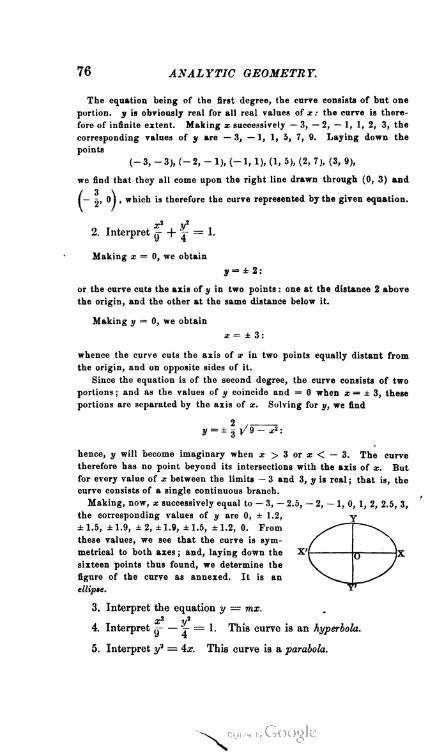
76 ANALYTIC GEOMETRY.
The equation being of the first degree, the curve consists of but one
portion, y is obviously real for all real values of x: the curve is there
fore of infinite extent. Making x successively —3,-2,-1, 1, 2, 3, the
corresponding values of y are —3, —1, 1, 5, 7, 9. Laying down the
points
(- 3, - 3), (- 2, - 1), (- 1, 1), (1, 5), (2, 7), (3, 9),
we find that they all como upon the right line drawn through (0, 3) and
(~ \' ') ' w''>cn '3 therefore the curve represented by the given equation.
2. Interpret if + J = 1-
Making x = 0, we obtain
y= ± 2:
or the curve cuts the axis of y in two points : one at the distance 2 above
the origin, and tho other at the same distance below it.
Making y = 0, we obtain
x = ± 3:
whenco the curve cuts the axis of x in two points equally distant from
the origin, and on opposite sides of it.
Since the equation is of the second degree, the curve consists of two
portions ; and as the values of y coincide and = 0 when x = ± 3, these
portions arc separated by the axis of x. Solving for y, we find
2y = ±3 /A-■ x*:
hence, y will become imaginary when x > 3 or x < — 3. The curve
therefore has no point beyond its intersections with the axis of x. But
for every value of x between the limits — 3 and 3, y is real ; that is, the
curve consists of a single continuous branch.
Making, now, x successively equal to — 3, — 2.5, — 2, — 1, 0, 1, 2, 2.5, 3,
the corresponding values of y are 0, ± 1.2,
± 1.5, ± 1.9, ± 2, + 1.9, ± 1.5, ± 1.2, 0. From
these values, we see that the curve is sym
metrical to both axes ; and, laying down the
sixteen points thus found, we determine the
figure of the curve as annexed. It is an
ellipse.
3. Interpret the equation y
4. Interpret g- — ~ = I . This curve is an hyperbola.
5. Interpret yl = 4x. This curve is a parabola.
THE RIGHT LINE. 77
6. Interpret y = x3 and y2 = x3. The first of these curves is
a cubic parabola ; and the second, a semi-cubic parabola.
7. Interpret x3 — (a — x) y* = 0. This is known as the Cissoid
of Diodes.
8. Interpret x2y* = {a? — y1) (b + yf. This is the Conchoid
of Nicomedes.
9. Interpret x = versin —1 y * — V'2 ry — y'. This is the Com
mon Cycloid.
10. Interpret y — sin x, the Curve of Sines ; y = cos x, the Curve
of Cosines ; and y = log x, the Logarithmic Curve.
Section II. — The Right Line.
THE RIGHT LINE UNDER GENERAL CONDITIONS.
74. In discussing the mode of representing the Right
Line by analytic symbols, we shall in the first place have
to determine the various forms of the equation which rep
resents any right line; that is, our problem will be to
represent the Right Line under general conditions only.
This accomplished, we shall then pass to the more partic
ular forms of the equation — those which represent the
Right Line under such special conditions as passing
through two given points, passing in a given direction
through one given point, etc.
75. In showing that a certain curve is represented by
a certain equation, we may proceed in either of two ways.
* This is the notation for an inverse trigonometric function, and is in this
ease read " the arc whose versed-sine is y." Similar expressions occur in
terms of the other trigonometric functions : as, x = sin _1 y ; x = tan -1 y ;
etc., read " x — the arc whose sine is y," " x = the arc whose tangent is y,"
and so on.

7s ANALYTIC GEOMETRY.
First, we may begin by assuming some fundamental
property of the curve, define the curve by means of it,
and, with the help of a diagram which brings it into rela
tion with elementary geometric theorems, embody it
in an equation between the co-ordinates of any point
on the curve — an equation from which all other prop
erties may be deduced by suitable transformations.
Or, secondly, we may begin without any geometric
assumptions except those on which the convention of
co-ordinates is founded; may take an equation of any
degree, in its most general form; and, by the purely
analytic processes of algebraic, trigonometric, or co
ordinate transformation, reduce the equation to such
simpler forms as will show us the species, figure, and
properties of the corresponding curve. The latter
method is the purely analytic one ; the former mingles
the processes of geometry and analysis.
76. In the present Book, both of these methods will
be applied in succession. It' will be natural to set out
from the geometric point of view : for in this way we
shall secure simplicity and clearness, by constantly
bringing the analytic formulae and operations to the
test of interpretation by a diagram. After the char
acteristic forms of the equation to any locus have been
obtained by the aid of geometry, and the beginner
has become familiar with their geometric meaning,
he may safely ascend to the higher analytic stand
point, and will be able to descend from it with some
real appreciation of the scientific beauty which it brings
to light.
We proceed to apply to the Right Line the two
methods mentioned, and shall follow the order which
has just been indicated.
\

EQUATION TO RIGHT LINE. 79
I. GEOMETRIC POINT OF VIEW : — THE EQUATION TO THE
RIGHT LINE IS ALWAYS OF THE FIRST DEGREE.
77m There are three principal forms of the equation
to the Right Line, arising out of the three sets of data
by which the position of the line is supposed to be deter
mined. Each of these will prove to be of the first
degree.
78. Equation to the Right Line in terms of its
angle with the axis of ac and its intercept on the
axis of y.—It is obvious, on inspecting the diagram, that
the position of the line DT is given f . ■
when the angle DTX* and the
intercept OD are given.
Let x and y denote the co-ordi
nates OM, MP of any point P on
the line. Let the angle DTX= a,
and let OD = b. Then, drawing
MR parallel to DT, we shall have
(Trig., 867)
OR : OM : : sin OMR : sin ORM.
That is, b— y : x : : sin a : sin (a — ai).
sin a , ,x + b;
sin (at — a)
sin aor, putting m = -.—; r ,
' * * sin (co — a) '
y = mx + 6:
which is the equation in the terms required.
s" The student will not fail to notice that the angle which a lino makes
with the axis of x is always measured, positively, from that axis toward
the left; an angle measured from the axis toward the right, is negative.
This principle holds true of the angle between any two lines.
An. Ge. 10.
80 ANALYTIC GEOMETRY.
Corollary 1.—In the equation just obtained, the axes
are supposed to have any inclination whatever. If the
axes are rectangular, w — 90° and m — tan a. Hence, in
y — mx + b,
when referred to rectangular axes, m denotes the tangent
of the angle which the line makes with the axis of x;
but when the equation is referred to oblique axes, m de
notes the ratio of the sines of the angles which the line
makes with the two axes respectively.
Remark.—In interpreting an equation of the form
y = mx + b, and tracing the line corresponding to the
values m and b have in it, account must be taken of the
signs of those constants. * The constant m will be posi
tive or negative according as the angle a is less or greater
than co. For m = -—^in -— : which is positive or neg-
sin (to — a)
ative upon the condition named, according to Trig., 829 ;
since a is supposed not to exceed 180°. The constant b
(Art. 49) will be positive or negative according as the
intercept on the axis of y falls above or below the origin.
Thus, in the case of the line in the diagram, m is
negative, and b positive.
If the axes are rectangular, the sign of m will be + or
— according as a is acute or obtuse. For, in that case,
m — tan « ; and the variation of sign is determined by
Trig., 825.
Corollary 2.—We can thus determine the position of a
right line with respect to the angles about the axes, by
merely inspecting the signs of its equation.
* The quantities m and b are constants, since they can have bat one
value for any particular right line. But the equation is true for any right
line, because we can assign to wt and b any values we please. They are
hence called arbitrary constants.
EQUATION TO RIGHT LINE. 81
If m is negative, and b positive, the line crosses the
axis of y above the origin, and makes with the axis of x
an angle greater than to : it therefore crosses the latter
at some point to the right of the origin, and so lies across
the first angle.
If m and b are both positive, the line lies across the
second angle.
If m and b are both negative, the line lies across the
third angle.
If m is positive, and b negative, the line lies across the
fourth angle.
[The student may draw a diagram and verify the last
three statements.]
Corollary 3.—If m = 0, we shall have sin a = 0
. • . a = 0, and the line will be parallel to the axis
of x.
Corollary 4.—If m — oo, sin [to — a) = 0 . • . a = a>,
and the line will be parallel to the axis of y.
If m = cc when the axes are rectangular, we shall
have tan a — oo . • . a = 90°, and the line will be per
pendicular to the axis of x : which is essentially the same
result as before.
Corollary 5.—If 6 = 0, the line must pass through the
origin. But, in that case, the equation becomes
y = mx:
which is therefore the equation to a right line passing
through the origin.
79. Equation to the Bight Line in terms of its
intercepts on the two axes.—The diagram shows that
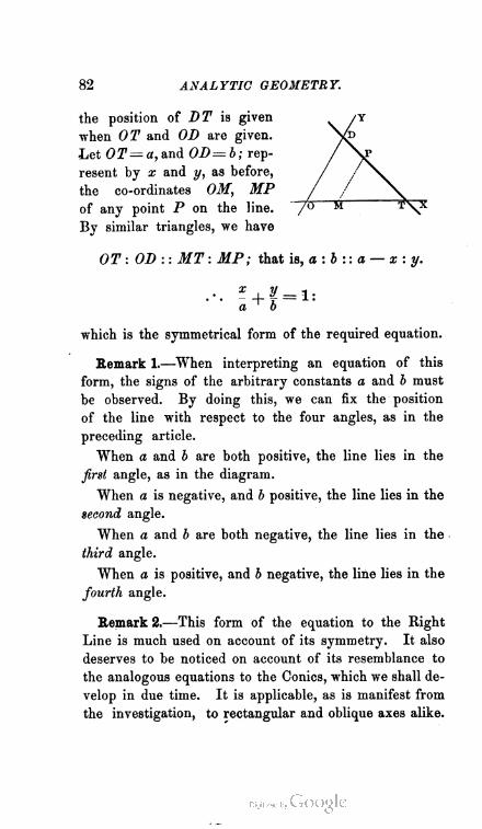
82 ANALYTIC GEOMETRY.
the position of DT is given
when OT and OD are given.
Let 0T= a, and OD=b; rep
resent by x and y, as before,
the co-ordinates OM, MP
of any point P on the line.
By similar triangles, we have
OT : OD : : MT : MP; that is, a : b : : a — x : y.
which is the symmetrical form of the required equation.
Remark 1.—When interpreting an equation of this
form, the signs of the arbitrary constants a and b must
be observed. By doing this, we can fix the position
of the line with respect to the four angles, as in the
preceding article.
When a and b are both positive, the line lies in the
first angle, as in the diagram.
When a is negative, and b positive, the line lies in the
second angle.
When a and b are both negative, the line lies in the
third angle.
When a is positive, and b negative, the line lies in the
fourth angle.
Remark 2.—This form of the equation to the Right
Line is much used on account of its symmetry. It also
deserves to be noticed on account of its resemblance to
the analogous equations to the Conies, which we shall de
velop in due time. It is applicable, as is manifest from
the investigation, to rectangular and oblique axes alike.

EQUATION TO RIGHT LINE. 83
SO. Equation to the Right Line in terms of its
perpendicular from the origin and the angle
made by the perpendicular with the axis of x.—
By examining the diagram, it
becomes evident that the po
sition and direction of DT are
given, if the length of OR per
pendicular to DT, and the angle
TOR which it makes with OX,
are given. Let OR=p; and let
the angle TOR = a, whence the
angle DOR = to — a. Then, a and b representing the
intercepts OT and OD as before, we have (Trig., 859)
a=_P_ ■ h = V
cos a cos (cu — «)
Substituting these values of a and b in the equation of
Art. 79, we obtain
x cos a y cos (to — «) ^
P P
Clearing of fractions,
x cos a + y cos (to — a) = p :
which is the equation sought.
Remark.—The co-efficients of x and y in the foregoing
equation are called the direction-cosines of the line which
the equation represents. In using this form of the
equation, it is most convenient to suppose that the
angle a may have any value from 0 to 360°, and that
the perpendicular p is always positive—that is, (Art. 50,
Note,) measured from 0 in such a direction as to bound
the angle. This convention can not be too carefully
remembered.
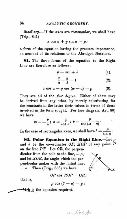
84 ANALYTIC GEOMETRY.
Corollary.—If the axes are rectangular, we shall have
(Trig., 841)
x cos a -\- y sin a = p:
a form of the equation having the greatest importance,
on account of its relations to the Abridged Notation.
81. The three forms of the equation to the Right
Line are therefore as follows:
y = mx + b (1),
5 + ? = \ <2>'
x cos a + y cos (a> — a) = p (3).
They are all of the first degree. Either of them may
be derived from any other, by merely substituting for
the constants in the latter their values in terms of those
involved in the form sought. For (see diagram, Art. 80)
we have
b P . A Pm = ; a = — ; o = ; r •
a cos a cos (to— a)
In the case of rectangular axes, we shall have b = . P .
& ' sin a
82. Polar Equation to the Right line.—Let f>
and 6 be the co-ordinates OP, XOP of any point P
on the line PT. Let OR, the perpen
dicular from the pole to the line, = p ;
and let XOR, the angle which the per
pendicular makes with the initial line,
i= a. Then (Trig., 858) we have
OP cos ROP=OR;
that is,
p cos (0 — a) — p:
is the equation required.

POLAR EQUATION TO RIGHT LINE. 85
Corollary.—If the initial line were perpendicular to the
right line, we should have a = 0, and the equation
would become
ft cos 0 = p :
the equation to a right line perpendicular to the initial line.
Remark.—In applying the equation of the present
article, it will be convenient to regard the sign of the
angle «. This will be + if the perpendicular OR falls
above the initial line; but — , if it falls below.
83. To trace a Right Line.—The most direct
method of solving this problem, consists in finding the
intercepts made by the line on the axes, and laying them
off according to any chosen scale of equal parts.
Hence, to trace a right line given by its equation :
Make the y and x of the equation successively — 0 : the
resulting values of x and y will be the intercepts on the
axis of x and of y respectively. Lay off on the axes
these intercepts, and the line drawn through their extremi
ties will be the line required.
Remark.—If the line is given by its polar equation,
we find its intercept on the initial line by making 0 = 0.
When this and the perpendicular from the pole are laid
off, we draw the line through their extremities.
Note.—This method fails when the line passes through the origin
or the pole, or is parallel to either axis. In the former case, in the
Cartesian equation, make x=l, construct the corresponding ordi
nate, and join its extremity to the origin ; in the polar system, lay
off the constant vectorial angle of the line. A parallel to either
axis must be drawn as such, at the distance its equation requires.
84. We add a few miscellaneous exercises on the
foregoing articles.
86 ANALYTIC GEOMETRY.
EXAMPLES.
1. Across which of the four angles does the line y — Zx + 5
lie?—the line y = — 6x + 2?— the line y = — 2x — 4? — the
line y = x — 1 ?
2. What is the situation and direction of the line y = x ?
3. Axes being oblique, what angle does the line y = x make
with the axis of x f — the line y = -f 2 ?
V 3
4. What is the direction of the line y = 4?
5. What is the direction of the line y — ^ + 6 ? What are the
intercepts made by the preceding lines on the axis of y ?
6. Trace the line y = bx + 3 ; — the line y — a; = 0.
7. Trace the lino % + | = 1 ; — the line § — | = 1.
8. Trace the line \x VZ +i y = 1.
9. What is the value of the angle a in the line of the previous
example?—of the angle u?—of the perpendicular pi [Here
cos a = i Vi ; cos (u — a) = i . ]
10. a: + i y = 3 is in the form x cos a + y cos (<■> — a) = p •"
determine the values of p, a, and w, and trace the line.
11. \ x l/3 + ^ y = 5 being referred to rectangular axes, find
the values of a and and lay off the line by means of them.
12. In which of the angles lie the lines 2 3 ~ ^' 3~2^~ ^'
f + f = -l,andf-* = l?
13. In which angle does the line | x y/Z — - y = 2 lie?
14. Trace the lines p cos (0 — 45°) = 8 and p sin 0 =— 6. What
is the value of a in the second line, and on which side of the initial
line is it measured ?
15. Find the intercepts of the line 5a; + 7y — 9 = 0, and trace
the line.
RIGHT LINE IN STRICT ANALYSIS. 87
II. ANALYTIC POINT OF VIEW:—EVERY EQUATION OF THE
FIRST DEGREE REPRESENTS A RIGHT LINE.
85. The most general form of the equation of the
first degree in two variables, is
Ax + By + C=0,
in which A, B and C are arbitrary constants, and may
have any value whatever. We propose to prove that
this equation, no matter what the values of A, B and C,
always represents a right line.
Solving the equation for y, we obtain
A _C
y—~Bx~~B'
That is, y is always equal to x multiplied by an arbitrary
constant, plus an arbitrary constant. In other words,
the equation is always reducible to the form
y = mx + b,
and therefore (Art. 78) always represents a right line.
86. A second proof of the same proposition, by means
of the trigonometric function which the equation implies,
is as follows :
Write the equation in the form (to which we have just
shown that it is always reducible)
y = mx + b :
in which m and b are merely abbreviations for the arbitrary
constants — -g and — -g . Now the equation, being true
for every point of its locus, must be true for any three
points x'y', x"y", x'"y'". Hence,
y' — mx' + b (1),
y" — mx» + b (2),
y"' = nuf" + b (3),
An. Ge. 11.
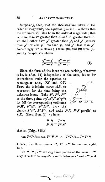
88 ANALYTIC GEOMETRY.
Supposing, then, that the abscissas are taken in the
order of magnitude, the equation y = mx + b shows that
the ordinates will also be in the order of magnitude ; that
is, if we take x" greater than x', and x'" greater than x",
we shall either have y" greater than y', and y'" greater
than y", or else y" less than y', and y'" less than y".
Accordingly, we subtract (1) from (2), and (2) from (3),
and by comparison obtain
y"-y' _ y"'-y"
x" —x'~ x'" — x"
Since the form of the locus we are seeking, whatever
it be, is (Art. 64) independent of the axes, let us for
convenience refer the equation to
rectangular axes, OX and OY.
Draw the indefinite curve AB, to
represent for the time being the
unknown locus. Take P', P", P"
as the three points x'y', x"y", x"'y"';
let fall the corresponding ordinates
PM, P'M", P"M"'; draw the
chords PP", P'P"; and make PR, P"8 parallel to
OX. Then, from (4), we have
P'R P"S .
P R— P" S;
that is, (Trig., 818,)
tan P"PR = tan P"P"S .-. P"PR=P"'P'S.
Hence, the three points P, P", P" lie on one right
line.
But P', P", P" are any three points of the locus. P"
may therefore be anywhere on it between P and P", and

RIGHT LINE IN STRICT ANALYSIS. 89
is independent * of them. Hence, as we may take the
points as near each other as we please, all the points of
the locus lie on one right line ; that is, the locus itself is
a right line.
871. A third proof of the same proposition is furnished
by transformation of co-ordinates.
Ax + By + C=0
being given for geometric interpretation, is of course
referred to some bilinear system of co-ordinates. Sup
pose the original axes to be rectangular, and let us
transform the equation to a new rectangular system
having the origin at the point x'y' .
To effect this, write (Art. 56, Cor. 3, cf. Art. 58) for
x and y in the given equation x' + x cos 6 — y sin 0
and y' + x sin 6 + y cos d. This gives us
(AcozO+ B&mf))x — {A sin0 — Bcos S)y + Ax' + B/ + C=0
as the equation to the unknown locus, referred to the
new axes.
Since x1, y', and d are arbitrary constants, we may
subject them to any conditions we please. Let us then
suppose that a/ and y' satisfy the relation
Ax' + By' + C=0,
and that the value of 0 is such that
A cos d + B sin 0 — 0 i. e. tan 0= s •
• This is essential to the argument. For three
points of a curve may lie on one right line, if the
third is determined by the other two. Thus, in the
annexed diagram, P' , P" , P'" are three points on
the curve AB ; yet they all lie on the right line
PP1". Tho reason is, that P" is determined by
joining P and P".
Tip M" M'" >'
90 ANALYTIC GEOMETRY.
The first of these suppositions means that the new origin
is taken somewhere on the unknown locus, since its co
ordinates satisfy the given equation; the second, that
the new axis of x makes with the old, an angle whose
Atangent is — -g- •
Applying these suppositions to the transformed equa
tion, we obtain, after reductions,
y = o.
Hence (Art. 49, Cor. 1) the locus coincides with the new
axis of x.
And, in general, since the equation Ax + By + C=0
can, upon the suppositions above made, always be reduced
to the form y = 0, we conclude that it represents a right
line, which passes through the arbitrary point x'y', and
makes with the primitive axis of x an angle whose tangent
is found by taking the negative of the ratio between the
co-efficients of x and y. That is to say, since these co
efficients are also arbitrary, Ax + By + C — 0 is the
Equation to any Right Line.
88. We have thus shown, by three independent demon
strations, that we can take the empty form of the General
Equation of the First Degree, and, merely granting that
it is to be interpreted according to the convention of co
ordinates, evoke from it the figure which it represents.
It must not be supposed, however, that we were ignorant
of the figure of the Right Line when we set out upon the
foregoing transformations. On the contrary, each of the
three demonstrations just given presupposes the figure
of the Right Line, and certain of its properties. What
we did not know is, that the equation Ax + By + C= 0
represents, and always represents, that figure.

EQUATION OF THE FIRST DEGREE. 91
It is important to call attention to this, because the
significance of the result just obtained is sometimes over
estimated ; and because the case of the Right Line is
different in this respect from that of any higher locus.
In the strictly analytic investigation of loci of higher
orders than the First, not even the figure of the curves
is presupposed, but is conceived as being learned for the
first time from their equations. But the whole scheme
of Analytic Geometry takes the figure and elementary
properties of the Right Line for granted ; as is obvious
from the nature of the convention of co-ordinates and
of the theorems for transformation.
89. Starting, then, from Ax + By + 0 = 0 as the
equation to the Right Line in its most general form, our
next step will naturally be to determine the meaning
of the constants A, B, and C. This meaning will be
found to vary according to the data by which we may
suppose the position of a right line to be fixed. In dis
cussing the Right Line from the geometric point of view,
we found that its equation assumed three forms, de
pending upon the three sets into which the data for its
position naturally fall. We shall now see that the gen
eral equation
Ax + By + (7=0
will assume one or another of those forms, according as
the constants in it are interpreted by one or another of
the sets of data.
OO. The first step toward a correct interpretation of
these, is to observe that the arbitrary constants in our
equation are but two:— a proposition which we might
infer from the fact that in an equation we are concerned
only with the mutual ratios of the co-efficients. But
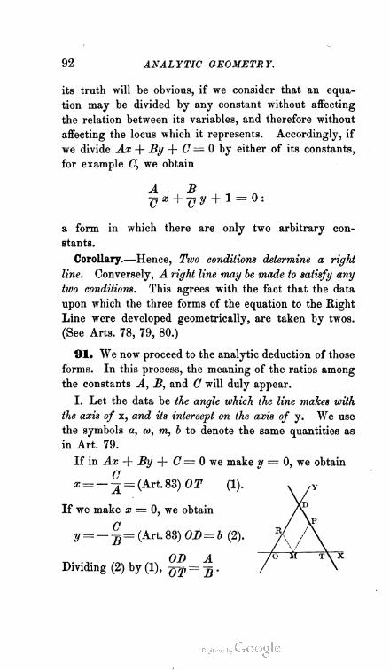
02 ANALYTIC GEOMETRY.
its truth will be obvious, if we consider that an equa
tion may be divided by any constant without affecting
the relation between its variables, and therefore without
affecting the locus which it represents. Accordingly, if
we divide Ax + By + C = 0 by either of its constants,
for example C, we obtain
a form in which there are only two arbitrary con
stants.
Corollary—Hence, Two conditions determine a right
line. Conversely, A right line may be made to satisfy any
two conditions. This agrees with the fact that the data
upon which the three forms of the equation to the Right
Line were developed geometrically, are taken by twos.
(See Arts. 78, 79, 80.)
91. We now proceed to the analytic deduction of those
forms. In this process, the meaning of the ratios among
the constants A, B, and C will duly appear.
I. Let the data be the angle which the line makes with
the axis of x, and its intercept on the axis of y. We use
the symbols a, w, m, b to denote the same quantities as
in Art. 79.
If in Ax -f- By + 0= 0 we make y = 0, we obtain
x =- ~ = (Avt. 83) OT (1). x /Y
If we make x = 0, we obtain
0 / V

MEANING OF THE CONSTANTS. 93
A sin a
Hence, (see Trig., 867,) -n = ——7 ; =—m (3).' v 6 ' B sin (a— <o) v '
From (2), we have -B =— -j; and from (3), J. =— mB=
. Substituting these values in the original equation,
we obtain
mC C
—x—by+C=0.
. • . y = mx + 6.
^ Q
Corollary 1.—By (3), m =— -g ; and by (2), b =— -g .
Hence, in the equation to a given right line the ratio
between the co-efficients of x and y, taken with a con
trary sign, denotes the ratio between the sines of the angles
which the line makes with the two axes: or, when the axes
are rectangular, it denotes the tangent of the angle made
with the axis of x ; and the ratio of the absolute term to
the co-efficient of y, taken with a contrary sign, denotes
the intercept of the line on the axis of y.
Corollary 2.—Hence, to reduce an equation in the
form Ax -f- By + C = 0 to the form y = mx + b, we
merely solve the equation for y.
II. Let the data be the intercepts of the line on the two
axes. Here a and b have their usual signification.
Making y = 0 in Ax + By + C = 0, we find as
before
x = -- = 0T=a (1). V,
Making x — 0, we obtain

94 ANALYTIC GEOMETRY.
C C
From (1), A=— ~; and from (2), B=— -r . Substi
tuting for A and B in the equation, and reducing,
-+£ = 1.a o
Corollary 1.—From (1) and (2), we see that the ratios
of the absolute term to the co-efficients of x and y re
spectively, taken with contrary signs, denote the intercepts
of the line on the axis of x and the axis of y.
Corollary 2.—To reduce Ax + By + C = 0 to the
x y
form- + ^- = l, we divide it by its absolute term, and,
if necessary, change its signs.
III. Let the data be the perpendicular from the origin
on the line, and the angle of that perpendicular with the axis
of x. We use p and a in the same sense as in Art. 80.
Making y and x successively equal to 0 in the general
equation, we obtain, as before,
(Trig., 859)P
cos a(1),
P^__ = 0^(Trig.,859)cos [(o_,a)
„ . 6'cosaFrom (1), A= — •
„ „ „ C cos (to—a)
From (2), B = j
Substituting for A and B in
the general equation, we have
C cos a
(2).
P
C cos (to — «)
P
y + C=Q:
x cos a + y cos (to — a) =p.

CONSTANTS IN TERMS OF DIRECTION-COSINES. 95
Corollary.—From (1) and (2) we learn that
A cos a
B cos (to — a) '
or, the ratio between the co-efficients of x and y, denotes
the ratio between the direction-cosines.
Remark.—The reduction of Ax + By + C= 0 to the
form x cos a + y cos (co — a) = p is of such importance
that we shall discuss its method in a separate article.
92. Reduction of Ax + By + C= 0 to the form
x cos a -j- y cos (co — a)— p.—The problem may be more
precisely stated : To find the values of cos a, cos (co — a),
and p, in terms of A, B, and C.
If, in the preceding article, we divide (1) by (2), we
find & = cos (<0.-a)m That i8> (Trig-j 845; IV ; 839,)
jfi. COS fit
B
-j = cos co + sin to tan a.
B—A cos co. • . tan a = ——A—= •
A sin to
1 A sin co
V(l+ tan2a) = i/(^2 2 ^LB cos a») '
Bcosa B sin co
cos (">— «)= ^ = 2 AjBcosw) "
Ccosa (Tsinw
P = ~ ^ =—^/(A'+B2— 2 AB cos co)
cos fit
Therefore, to make the required reduction, Multiply the
sin co %
equation throughout by ^j-2 + &_2AB cos co) '
9 The following elegant solution of this problem is by Salmon : Conic
Sections, p. 20 :
" Suppose that the given equation when multiplied by a certain factor
R is reduced to the required form, then RA = cos a, MB = cos ($. But it
can easily be proved that, if a and /3 be any two angles whose sum is q}
we shall have
9G ANALYTIC GEOMETRY.
Remark.—Since we have agreed always to consider p
a positive quantity, it may be necessary to change the signs
of the given equation, before multiplying, so that its abso
lute term when transposed to the second member may be
positive.
Corollary 1.—If the axes are rectangular, we shr.il
have
A . B
cos a = + B2y, sin « - + ^ ;
C
P—'v'(A' + &)'
Accordingly, Ax + By + C = 0 is reduced to the form
x cos a + y sin a = p, by dividing all its terms by V A2-\-B2,
after the necessary changes of sign.
Great importance pertains to the transformation ex
plained in this corollary. The general reduction to
x cos a -f- y cos (to — a)~P is of comparatively infre
quent use.
Corollary 2.—From the values of p above obtained, we
learn that the length of the perpendicular from the origin
upon the line Ax -f- By -f- C= 0 is
cos2 a + cos2 3 — 2 cos a cos [5 cos w = sin2 u.
Hence, R2 (A2 + Bl — 2 ^tif cos a) = sin2 u ; and the equation reduced to
the required form is
A sin 6) B sin 6>»'(A2 + .B2-2 4JBcoscj) x + y'{A2 + B^2 ABeoau) 3
C sin w
+ rtiH'ff -2 JScos u)
And we learn that
A sin o B sin 6)
f'( ,i2 + fi2~2 XBcoFu) ' y'(A2 + £2"-:r2/lBcos u)
arc respectively the cosines of the angles that the perpendicular from the
origin on the line Az+By + C=0 makes with the axes of x and y; and
C sin uV(A*+ B' — 2 ABcos^ is the lenEth of that perpendicular."
POLAR EQUATION BY ANALYSIS. 97
Csin to
~ v {A2 + B*—2AB cos to) '
and that this length becomes
0
when the axes are rectangular.
93. Polar Equation to tbe Right Line, deduced
analytically.—The polar equation may be obtained
from the Cartesian as follows : Let Ax + By -f- 0'= 0,
referred to rectangular axes, be reduced to the form
x cos a + y sin a = p.
Transforming to polar co-ordinates, we have (Art. 57,
Cor.) x = p cos 0, and y — p sin 6 : and the equation
becomes
p (cos 6 cos a + sin 0 sin a) =p;
that is, pcos(0 — a)=p,
the equation of Art. 82.
Corollary.—Transforming the original equation to
polars, we have
p (A cos 6 + B sin 0) + C= 0.
Hence, an equation in the form p (A cos d + 5 sin 8) =C
may be reduced to the form p cos (d — a) =p by dividing
each term by y/Ai-\- B2.
94. Before advancing to the more particular forms
of the equation to the Right Line, the student should
make sure of having mastered the general ones which
precede, and the principles which have been developed in
the course of the discussions just closed. To this end,
let the following exercises be performed.

98 ANALYTIC GEOMETRY.
EXAMPLES.
1. Transform 3x — by + 6 = 0 to y = 0. What is the angle
made by the new axis of x with the old ?
2. What angle does the line Sx + )2y + 2 = 0 make with the
axis of x t What is the length of its intercept on the axis of y J
In which of the four angles does it lie?
3. Find the intercepts of the line x -\- Sy — 3 = 0.
4. Find the ratio between the direction-cosines of the right line
2x + Zy + 4 = 0, u being = 60°.
5. What is the tangent of the angle made with the axis of x
by the perpendicular from the origin on 3x — 2y — 6 = 0?
6. Reduce all the equations in the previous examples to the
form x cos a + y sin a— py and determine a and p for each line.
7. Reduce 3.r + 4y = 12 to the form x cos a -\- y cos (u — a)~P-
What are the values of a and (u — a), supposing a successively
equal to 30°, 45°, 60°, and sin"1 f ?
8 Find the length of the perpendicular from the origin on
3x + 4y + 12 = 0, under the several values of a last supposed.
9. Find the length of the perpendicular from the origin on
Zx — 4y — 12=0, axes being rectangular.
10. Reduce 2 p cos 6 — 3 p sinfl = 5 to the form p cos (6 — a) =p.
What are the values of a and p ?
THE BIGHT LINE UNDER SPECIAL CONDITIONS.
95. Equation to the right line passing through
Two Fixed Points.—Let the two points be x?y', x"y".
Since they are points on a right line, their co-ordinates
must satisfy the equation
Ax + By + C= 0 (1),
and we therefore have
Ax' +By' +O=0
Ax" + By"+ C=0
(2) ,
(3) .
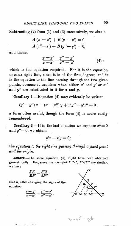
RIGHT LINE THROUGH TWO POINTS. 99
Subtracting (2) from (1) and (3) successively, we obtain
A(x -x') + B(y -«/')=0,
A(x"-x') + B(1,"-y')=0,
and thence
y — y' y" — y'
x" — x>(4):
which is the equation required. For it is the equation
to some right line, since it is of the first degree ; and it
is the equation to the line passing through the two given
points, because it vanishes when either x' and y' or x"
and y" are substituted in it for v and y.
Corollary 1.—Equation (4) may evidently be written
(y' — y") x—(x'— x") y + x'y" — y'x" = 0 :
a form often useful, though the form (4) is more easily
remembered.
Corollary 2.—If in the last equation we suppose x"= 0
and y"~ 0, we obtain
y'x — x'y = 0 :
the equation to the right line passing through a fixed point
■and the origin.
Remark.—The same equation, (4), might have been obtained
geometrically. For, since the triangles PRP/} P'SP" are similar,
we have
Pit _P'S
RP' ~ SP" '
that is, after changing the signs of the /e^\p'
equation, / ,/ a/\Y"

100 ANALYTIC GEOMETRY.
It is worth while to place the analytic and geometric proofs thus
side by side, in order to make sure that the geometric meaning of
all the symbols in the equations developed, shall be clearly under
stood.
96. Angle between two right lines given by
their equations.—All formulae for angles are greatly
simplified by the use of rectangular axes. We therefore
present the subject of this article first in the form which
those axes determine.
Let the two lines be y = mx + h
and y = m'x + V ; and let <p = the
angle between them. From the dia
gram, <p — a' — a ; and we have
(Trig., 845, vi)
tan a1 — tan a
a ^ tan a tan c'
m' — m
= rr , (Art. 78, Cor. 1).1 + mm' v ' >
Corollary 1.—If the equations were given in the form
Ax + By + C=0, A'x + B'y + C = 0, we should have
A A'
(Art. 91, 1, Cor. 1) m = — -g , and m' = — -^7 . Hence,
in that case,
AB' — A'B
tan?- AA> + BB''
Corollary 2—If f — 0 or jr, tan <p = 0 ; and we have
m> — m = 0 or AB' — A'B = 0 :
the condition that two right lines shall be parallel.
Corollary 3.—If <p = 90°, tan <p = oo ; and we have
1 +W= 0 or AA' + BB' = 0 :
the condition that two right lines shall be mutually perpen
dicular.
ANGLE BETWEEN TWO RIGHT LINES. 101
97. Angle between two lines, axes being; oblique.—From
Art. 92 we shall have cos a = , f sln " . and cos a'=
y (A' -t- Bl — 2A B cos u) '
,4' sin"TP7^ £/2-2 A'B' cos 6,)- ^nce (frig., 838)
. . B'— ,4'cosu
V(4'a + 2i'a-2 4'iJ'cos «) '
-B — ^4. cos u
Therefore (Trig., 845, in and iv)
. (AB'—A'B) sin a
J AA/ + BjB/ — (AB'+A'B) cos 6)
Whence (Trig., 839)
(AB' —A'B)smutan <? — —
AA' + BBT- (AB' + A'B) cos u '
a formula which evidently becomes that of Art. 96, Cor. 1, ifu=90°.
Corollary 1—The condition that the two lines shall be parallel,
is
AB' — A'B=0:
from the identity of which with the condition of Art. 96, Cor. 2,
we learn that the condition of parallelism is independent of the value
of The same follows from the fact that the condition itself is
not a function of u.
Corollary 2—The condition that the lines shall be perpendicular
to each other, is
AA' + BB' - (AB' + A'B) cos <j = 0.
98. Equation to a right line parallel to a given
one.—Let the given line be y = mx-\-b. The required
equation will be of the form
y = mix + V.

102 ANALYTIC GEOMETRY.
But in this, the condition of parallelism (Art. 96, Cor. 2 ;
Art. 97, Cor. 1) gives us ml = m. The required equation
is therefore
y = mx + V.
Corollary.—If the given line were Ax-\-By-\- C=0,
the equation would be of the form A'x + B'y + C* = 0.
A C
In that case, m =— jj , and 6' = — ^ . The required
JSC"
equation would therefore be, after writing C" for -g/- ,
^r + 5y+ O"=0.
From this we infer that the equations to parallel right lines
differ only in their constant terms.
99. Rectangular equation to a right line per
pendicular to a given one.—The equation will be of
the form y= m'x + b', in which w! is determined by the
condition (Art. 96, Cor. 3)
1 + mm' — 0.
Hence, m' — — — ; and the equation is
y = — — x + b'.
Corollary.—When the given line is Ax-\-By-\- O—0,
the equation to its perpendicular is (Art. 91, I, Cor. 1)
Ay — Bx + Oi = 0.
Hence, if two right lines are perpendicular to each other,
their rectangular equations interchange the co-efficients of
x and y, and change the sign of one of them.
SYMMETRIC EQUATION TO RIGHT LINE. 103
1.00* Equation to a right line perpendicnlar to a given
one, axes being obliqne.—From the condition of perpendicularity,
(Art. 97, Cor. 2,)
A' (A — B cos o) + B' (B— A cos u) = 0
A' B— A cos u
Hence, frr — —; t-, j' B' A — B cos u
and the required equation (Art. 91, I, Cor. 1) is
(A — B cos u) y — (B — A cos ") x + C% = 0.
101. Equation to a right line parallel to a
given one, passing through a Fixed Point.—By
Art. 98 we have the form of the equation,
y = mx + V (1).
Calling the fixed point x'y', we therefore obtain
y' = mx' + V :
. • . b' =y' — mx'.
Substituting for b' in (1), the equation sought is
y — y' = m (x — x').
Corollary 1.—If in this equation we suppose m indeter
minate, the direction of the line is indeterminate ; and we
have th.e*equation to any right line passing through a fixed
point.
Corollary 2.—Let sin a : sin co = k, and sin (co — «) ;
sin co = h. Then k : h ^ sin a : sin (co ■— a) = m; and
the equation may be written. ',
y — y' x — x'
~~~k^=~~7T>
or, if we denote either of these equal ratios by I,
y — y' _ a — s' _
k - h ~l:
An. Ge. 12.
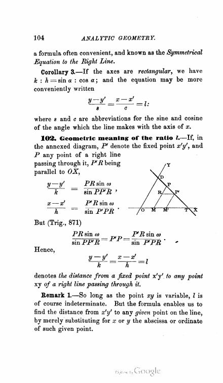
104 ANALYTIC GEOMETRY.
a formula often convenient, and known as the Symmetrical
Equation to the Rigid Line.
Corollary 3.—If the axes are rectangular, we have
k : h = sin a : cos a ; and the equation may be more
conveniently written
y —y'_x — x'
8 C
where s and c are abbreviations for the sine and cosine
of the angle which the line makes with the axis of x.
102. Geometric meaning of the ratio /.—If, in
the annexed diagram, P' denote the fixed point x'y', and
P any point of a right line
passing through it, PR being
parallel to OX,
y—y' PR sin 10
~k~ = sin PP'R '
x — x' PR sin (i>
h ~~ sin PPR
But (Trig., 871)
PR sin a PR
PP
Hence,
sin PPR ~* " — sin PPR
y — y' x — x'
denotes the distance from a fixed point x'y' to any point
xy of a right line passing through it.
Remark 1,—So long as the point xy is variable, I is
of course indeterminate. But the formula enables us to
find the distance from x'y' to any given point on the line,
by merely substituting for x or y the abscissa or ordinate
of such given point.

LINE CUTTING ANOTHER AT GIVEN ANGLE. 105
Thus, supposing the given point of the line to be x"y",
we should have (assuming the axes for convenience to be
rectangular)
x" - x'
Squaring both sides of these equations, adding, and
remembering (Trig., 838) that s2+ c2 = l, we obtain
p = (x» — x')2 + (y" — y'f :
which agrees with the formula (Art. 51, I, Cor. 1) for
the distance between two given points.
Remark 2.—The signs + and — in connection with I
denote distances measured along the line in opposite di
rections from x'y'. Thus, if + I were measured in the
direction P'D, — I would be measured in the direction
P' T; and vice versa. Speaking with entire generality,
+ I must be laid off from x'y' in the positive direction
of the line (Art. 50, Note), and — I in the negative.
103. Rectangular equation to a right line
passing through a Fixed Point, and cutting a
given line at a Given Angle.—Let the given line be
y = mx + b, and let 0 = the given angle. The equation
sought (Art. 101, Cor. 1) is of the form
y— y'=m' {x — xf),
in which m' is to be determined from the conditions of the
problem.
The line in question obviously makes with the axis of x
an angle a' — a + 0. Hence, (Trig., 845, v,)
; m + tan 0
m =1— mtan0 '

106 ANALYTIC GEOMETRY.
Substituting this value for m', the required equation is
m + tand
Corollary 1.—Dividing both terms of m' by tan 0, this
equation may be written
m cot 6 + 1
y-lt= cot 0-m C*-^-
Accordingly, if 0 = 90°, it becomes
y—y>=—— (x—xf):
the equation to a right line passing through a fixed point,
and perpendicular to a given line.
Corollary 2.—By substituting for — m its value A : B,
we obtain
as the equation to the perpendicular of Ax-\-By ~f-C=0,
passing through x'y' : the co-efficients of which evidently
satisfy the criterion of the corollary to Art. 99.
lO-l. Kqnntion to a right line passing through a Fixed
Point and cutting a given line at a Given Angle, axes being
oblique Let the given line be Ax -{-By +C= 0. Since </= a + 0,
e = a' — a.
By putting for mf its value, the required equation assumes the
form
A'y — y' = — -]p(x—x').
From Art. 97, we have
(AB' — A'B) sin 6)tan 6-
' AA' + BB' — (AB' + A'B) cos u '
therefore
A' A sin u — (B — A cos a) tan 8
W ~~ B sin u + {A — B cos a) ten 0 '
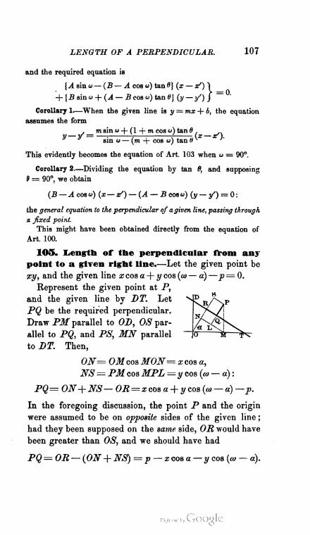
LENGTH OF A PERPENDICULAR. 107
and the required equation is
{A sin u — (B — A eos a) tanO] (x — x') "1
+ {B sin a + (A — B cos u) tan 8} {y — /) J =
Corollary 1.—When the given line is y = mi + 4, the equation
assumes the form
, msin <•> + (1 + m cos <•>) tan 8 ,
2/ — y = —: 7 i 7, (x — x).sin u — (m-\- cos u) tan w
This evidently becomes the equation of Art. 103 when u = 90°.
Corollary 2—Dividing the equation by tan fl, and supposing
9 = 90°, we obtain
(B — Acosu) (x—x/) — (A — B cosu) (y — = 0:
the general equation to the perpendicular of a given line, passing through
« fixed point.
This might have been obtained directly from the equation of
Art. 100.
105. Length of the perpendicular from any
point to a given right line.—Let the given point be
xy, and the given line x cos a + y cos (co — a) —p= 0.
Represent the given point at P,
and the given line by DT. Let
PQ be the required perpendicular.
Draw PM parallel to OD, OS par
allel to PQ, and PS, MN parallel
to DT. Then,
OiV= OM cos MON= x cos a,
NS= PM cos MPL =y cos (co — a) :
PQ= ON-\-NS— OR= xcosa + y cos (to — a)—p.
In the foregoing discussion, the point P and the origin
were assumed to be on opposite sides of the given line ;
had they been supposed on the same side, OR would have
been greater than OS, and we should have had
PQ= OR—(ON+ NS) =p — xcosa—ycoa [co — a).

108 ANALYTIC GEOMETRY.
Hence, if a perpendicular be let fall from any point xy to
the line
x cos « + y cos (to — a) —p = 0,
its length will be
± (x cos a + y cos (to — a) —p)
according as the point and the origin lie on opposite sides
of the line, or on the same side.
Remark—The student will observe that we here use the same
symbols xy to denote the co-ordinates of the point from which the
perpendicular is dropped, and those of any point on the given line.
But it must not be supposed that the xy of the point and the xy
of the line have necessarily the same values. Generally, of course,
they have not; for the point from which the perpendicular falls,
is generally supposed not to be a point on the line. It may be; and
when it is, the length of the perpendicular vanishes. Hence, sup
posing the quantity x cos a -\-y cos (u — a) —p to denote the length
of the perpendicular from xy on a given line, the equation
X cos a + y cos (u — a) — p = 0
signifies that the point lies somewhere on the line in question.
The double use of xy may cause some confusion at first, but its
advantages more than compensate for the attention required to
overcome this.
Corollary 1.—If the axes are rectangular, the length
of the perpendicular is
± (x cos a -\- y sin a —p)
according as the point and the origin lie on opposite sides
of the line, or on the same side.
Corollary 2.—The length of the perpendicular from xy
on the line Ax + By + C= 0 (Art. 92 cf. Cor. 1) is
(Ax + By+C) sin to Ax+By+C
± + 2 AB cos to) or * V(^2+-52)
according as the axes are oblique or rectangular.
POINT OF INTERSECTION. 109
Corollary 3.—The perpendicular from a point on the
same side of a line as the origin must have the same
sign as p. But we have agreed (Art. 80, Rem.) that p
shall always be positive; and we have seen that the per
pendicular changes sign in passing from one side of the
line to the other. Hence, Perpendiculars falling on the
side of a line next the origin are positive; and those falling
on the side remote, are negative.
106. To find the point of Intersection of two
right lines given by their equations.—Eliminate
between the equations to the two lines : the resulting
values of x and y (Art. 62) are the co-ordinates of the
required point.
Thus, in general, the lines being Ax + By -f- C— 0
and A'x + B'y + C = 0, we have
BC'— B'C OA' — C'A
x~ AB' — A'B> y~AB' — A'B
as the co-ordinates of the common point.
107. Equation to a right line passing through
the intersection of two given ones.—If we multiply
the equations to two given lines each by an arbitrary
constant, and add the results, thus :
I \Ax + By+C) + m (A'x + B'y + C) = 0,
the new equation will represent a right line passing
through the intersection of the lines Ax + By -f- C= 0
and A'x + B'y + C"=0.
For it manifestly denotes some right line, since it is
of the first degree. Moreover, it is satisfied by any
values of x and y that satisfy Ax -\- By + C= 0 and
A'x + B'y -f- C?= 0 simultaneously ; for its left member
must vanish whenever the quantities Ax + By + C and

110 ANALYTIC GEOMETRY.
A'x + B'y + C are both equal to zero. That is, it
passes through a point whose co-ordinates satisfy the
equations of both the given lines. But such a point
(Arts. 62, 106) is the intersection of the two lines.
Corollary.—By varying the values of the constants I
and m, we can cause the above equation to represent
as many different lines as we please, all passing through
the intersection of the two given ones.
Remark.—The truth of the above equation is inde
pendent of co, and of the form of the equations to the
given lines. This is manifest from the method by which
it was obtained. It may therefore, when convenience
requires, be written
I {x cos a-\- y cos (co — a) —p }
-\-m{x cos ft + y cos (co — ^3) —p'}
or
I (x cos a -f y sin a — p) -f m (x cos /? + y sin /3 —p') = 0.
108. meaning' of the equation L + kL' — O.—If
we put k — m : I, and represent by L and L' the
quantities which are equated to zero in the equations
of the two given lines, the equation of the preceding
article becomes
L + kL' = 0.
We shall now prove that this is the equation to any right
line passing through the intersection of two given ones. *
* The beginner may suppose that this has been done already, in the
preceding article. But we merely proved there, that the equation may
represent an infinite number of lines answering to the given condition.
Now, that an infinite number of lines is not the same as all the lines
passing through the intersection of two others, is evident. For between
two intersecting right lines there are two angles, supplemental to each
other, in each of which there may be an infinite number of lines passing
through the common point.
LINE THROUGH INTERSECTION. Ill
Let d = the angle made with the axis of x by the line
which the equation represents. Then (Art. 91, 1, Cor. 1)
sin d A -f kA'
sin (co — d) ~~B + kB> '
Therefore
(A + kA') sin co
tan 9 ~ (A cos to—B) + k (A' cos'w-^ '
Hence, as k may have any value from 0 to oo, and
be either positive or negative, tan 0 may ha.ve any
value, either positive or negative, from 0 to oo. That
is, the equation is consistent with any value of 6 what
ever.
Therefore, if L = 0 and L' = 0 are the equations to
two right lines,
L + kL' = 0
is the equation to any right line passing through the
intersection of the two.
Corollary 1.—The equation to a particular line inter
secting two others in their common point, is formed
from the above by assigning to It such a value, in terms
of the conditions which the line must satisfy, as the
relation L + kL' = 0 implies.
Thus, if the condition were that the intersecting line
make with the axis of a; a given angle = 0, we should
have, from the value of tan 6 above,
A sin a) — (^4. cos co — B) tan 0
k=— A'smoj ^(A'cosw ^B')iim~d '
or, in case the axes were rectangular,
A + B tan 0
k = ~ A' + B't&nd'
An. Ge. 13.

112 ANALYTIC GEOMETRY.
If the condition were that the intersecting line pass
through a fixed point x'y', we should have
(Ax1 + By' +C) + k {A'x* + B'y' + C) = 0 :
Ax>+By'+C
•'■ 10 — A'x' + B'y' + C" •
Corollary 2.—The sign of ir has a most important
geometric meaning. Obviously, in order to change its
sign, a quantity must pass through the value 0 or oo.
Now if k = 0, we have by Cor. 1
A + B tan 6 = 0 . • . tan 0 — — ^ .
And if k — oo,
A'A' + ^' tan 0 = 0 . • . tan 0 = — -g7 .
That is, (Art. 91, 1, Cor. 1,) a< the instant when k changes
sign, the line which passes through the intersection of two
given ones coincides with one of them. Hence, of the lines
L -f- kU = 0 and L —kU = 0, one lies in the angle be
tween L = 0 and U — 0 supplemental to that in which
the other lies.
It now remains to determine which of these supple
mental angles corresponds to -f k, and which to — k.
If the two lines are x cos a^-y cos {to — a) —p = 0 and
zcos/? + 2/cos(«>—^3) —jp'=0, we shall have
x cos a -\- y cos (to — a) — p
x cos ft + y cos (a> — /5) — '
that is, (Art. 105,) one of the geometric meanings of k is,
the negative of the ratio between the perpendiculars let fall
on two given lines from any point of a line passing through
their intersection. Hence, when k is positive, those per
pendiculars have unlike signs ; and when k is negative,
their signs are like. That is, (Art. 105, Cor. 8,) the per
pendiculars corresponding to + k fall one on the side of
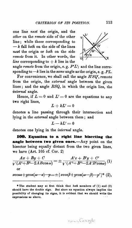
CRITERION OF ITS POSITION. 113
one line next the origin, and the
other on the remote side of the other Y
line ; while those corresponding to
— k fall both on the side of the lines
next the origin or both on the side .
remote from it. In other words, the
line corresponding to + k lies in the
angle remote from the origin, e.g. PL'; and the line corre
sponding to—k lies in the same angle as the origin, e. g. PL.
For convenience, we shall call the angle R'SQ', remote
from the origin, the external angle between the given
lines ; and the angle BSQ, in which the origin lies, the
internal angle.
Hence, if L = 0 and L' = 0 are the equations to any
two right lines,
L + kL' = 0
denotes a line passing through their intersection and
lying in the external angle between them ; and
L — kU = 0
denotes one lying in the internal angle.
109. Equation to a rigbt line bisecting the
angle between two given ones.—Any point on the
bisector being equally distant from the two given lines,
we have (Art. 105 cf. Cor. 2)
Ax + By + 0 ^ A'x + B'y + C
l/(A2+B2—2ABcos(o) ~ ± ^(A't+B'2—2A'B'cobw) W
or
a;cosa+?/cos(w—a)—p=±{xcos^-\-ycos(a»—ft)—p'}* (2),
* The student may at first think that both members of (1) and (2)
should hare the double sign. But since an equation always implies the
possibility of changing its signs, it is evident that we should write the
expressions as above.
114 ANALYTIC GEOMETRY.
according as the given lines are Ax + By + C= 0 and
A'x + + C = 0 or a; cos a -f «/ cos («j — a) —p = 0
and a: cos ft + y cos (w — /3) —p' — 0. Expressions (1)
and (2) are the principal forms of the required equation.
Corollary 1.—When the axes are rectangular, the
equation becomes
Ax + By + C A'x + B'y + C
>/(A2 + B-) - ~ V(An + B'2) W
or
x cos a -f- «/ sin a —p — ± (x cos ft + sin ft—p1) (4).
Corollary 2.—Expressions (1), (2), (3), (4) are evidently
in the form L ± kL' = 0. Hence (Art. 108, Cor. 2)
there are two bisectors: one lying in the external angle
of the given lines, and the other in the internal. For
the sake of brevity, we shall call the former the external
bisector ; and the latter, the internal bisector.
Corollary 3.—If we put, as we conveniently may,
a~x cos a + y cos (<u — a) —p,
ft = x cos ft -j- y cos (<u — /5) — p',
expressions (2) and (4) will be included in the brief and
striking form
f a±ft = 0.
Hence, if a = 0, ft — 0 are the equations to any two right
lines, the line
a + ft ■= 0
bisects the external angle between them ; and the line
a — ft = 0
bisects their internal angle.

BISECTOR OF ANGLE. 115
Caution.—From the proposition just reached, the stu
dent is apt to rush to the conclusion that
L ± L' = 0
is the equation to the bisector of the angle between the
lines L = 0 and U= 0, without regard to the values of
L and L'. This is a grave error. It assumes that the
value of k, in the case of a bisector, is always ± 1.
When the equations to two lines are in terms of the
perpendicular from the origin and its angle with the
axis of x ; that is, when L = x cos a + y cos (w— o) —p
and L' = x cos /3 + y cos {to — /3) — p', k = ± 1 . But
from equation (1) we have
l/(A2 + B2— 2AB cosw)
k—± y{An + B'1 — 2 A'B' cos to) :
which is obviously not in general equal to ± 1. The
condition that it shall have that value is
A2 + B2 — 2 AB cos co = A'2 + B'2 — 2 A'B' cos w
or, when the axes are rectangular,
. A2 + B2=A'2 + B'2.
Corollary 4.—If we denote by r the particular value
which k assumes in the case of a bisector, then
L + rL' = 0
represents the external, and
L — rl! = 0
the internal bisector of the angle between the lines L= 0
and L' = 0.

116 ANAL YTIC GEOMETR Y.
In these expressions, r is to be determined from the
relation
\/(A 2 + B 2 — 2 A B cos w)
r^± y/(An + B'2 — 2 A'BUoT^) '
which, in case the axes are rectangular, becomes
x/(A' + B*)
r-~V{An + Bn)'
HO. Equation to a right line situated at in
finity.—To assume that a right line is at an infinite
distance from the origin is to assume that its intercepts
on the axes are infinite. Hence, we have
0 c
— — oo ana — -g = oo.
That is, supposing C to be finite,
A = 0 and B = 0.
The required equation is therefore
0x + Oy + C=0:
in which C is finite. We shall cite it in the somewhat
inaccurate but very convenient form
0=0.
Remark.-—The student will of course remember that a line at
infinity is not a geometric conception at all— in fact does not exist,
in any sense known to pure geometry. As an analytic conception,
however, it has important bearings; and the equation just obtained
is useful in some of the higher investigations of curves.
111. Equations of Condition.—When elements of
position and form sustain certain geometric relations to
each other, the constants which enter their analytic equiv
alents must sustain corresponding relations. In other
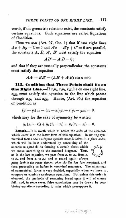
THREE POINTS ON ONE RIGHT LINE. 117
words, if the geometric relations exist, the constants satisfy
certain equations. Such equations are called Equations
of Condition.
Thus we saw (Art. 97, Cor. 1) that if two right lines
Ax + By + 0= 0 and A'x + B'y + C' = 0 are parallel,
the constants A, B, A', B' must satisfy the equation
AB' — A'B = 0;
and that if they are mutually perpendicular, the constants
must satisfy the equation
AA! + BB' — (AB' + A'B) cos a = 0.
113. Condition that Three Points shall lie on
One Right Line.—If £,«/,, t^fa x$3 lie on one right line,
x^y3 must satisfy the equation to the line which passes
through and x$y2. Hence, (Art. 95,) the equation
of condition is
(#i — 2/2) *3 — (x, — x2) y3 + xty2 — yxx2 = 0 :
which may for the sake of symmetry be written
y\ O2 — z3) + y2 te) — *i) + 2/3 (*i — z2) = 0-
Remark.—It is worth while to notice the order of the elements
which enter into the latter form of this equation. In writing sym
metrical forms, the analogous symbols must be taken in a fixed order,
which will be best understood by conceiving of the
successive symbols as forming a circuit, about which -s?"
we move according to the annexed diagram. Thus, XH \
as in the last equation, we pass from xt to x2, from x2 fc^—j'V
to x3, and from x3 to xY\ and so round again: always
going lack to the first element when the list has been completed, and
then proceeding as before in numerical succession. The advantage
of symmetrical forms is very decided, especially when we have to
compare or combine analogous equations. But unless this order is
observed, the methods of reasoning based upon it will of course
fail ; and, in some cases, false conclusions may be drawn by com
bining equations according to rules which presuppose it

118 ANALYTIC GEOMETRY.
113. Condition that Three Right Lines shall
meet in One Point.—If three lines Ax + By +(7= 0,
A's + -B'y + C" = 0, A"x + + C" = 0 pass through
the same point, the co-ordinates of intersection for the
first two must satisfy the equation to the third. Hence,
(Art. 106,) the required condition is
A" (BC'—B'C) +B" (CA'—C'A) + C" (AB'—A'B)= 0.
114. A condition often more convenient in practice,
is derived from the principle of Arts. 107, 108. For
if three right lines meet in one point, the equation to
the third must be in the form of the equation to a right
line passing through the intersection of the first and
second. Therefore, supposing the three lines to be
L = 0, L' = 0, L" = 0, we can always find some three
constants, I, m, and — n, such that
— nL"= lL + mL',
where — n may be either a positive or a negative quan
tity. Hence, the condition is
lL + mL' + nL"=0.
That is, three right lines meet in one point when (heir
equations, upon being multiplied respectively by any^
three constants and added, vanish identically. %
Remark.—For brevity, we shall often refer to three
right lines passing through one point by the name of
convergents.
115. Condition that a Morable Right lane shall
pass through a Fixed Point.—Comparing Art. 101,
Cor. 1 with Art. 91, I, Cor. 1, it is evident that the
equation to a right line passing through a fixed point
whose coordinates are I : n and m : n, may be written
A (nx — T) + B {ny — m) = 0.

MOVABLE LINE THROUGH FIXED POINT. 119
And comparing this with the general equation to a right
line, we have
— (IA + mB) = nC.
The required condition is therefore
IA + mB + nC=0.
Hence, a movable right line passes through a fixed point, so
long as the co-efficients in its equation suffer no change in
consistent with their vanishing when multiplied each by a
fixed constant and added together.
Corollary.—The criterion of this article may be other
wise taken as the condition that any number of lines
shall pass through one point. For every line whose
co-efficients satisfy the equation IA + mB + nC = 0,
must pass through the point I : n, m : n.
116. In this connection also, Art. 108 furnishes us
with a second condition. For, since we may always
regard a fixed point as the intersection of two given
right lines, the most general expression for a right line
passing through a fixed point is
L + kL' = 0.
By writing L and L' in full, and collecting the terms,
this becomes
(A + kA') x + (B + kB') y + (C + kC) = 0.
Now the condition that the line shall be movable is that
k be indeterminate. Hence, a movable right line passes
through a fixed point lohenever its equation involves an
indeterminate quantity in the first degree.
Corollary.—The co-ordinates of the fixed point may
be found by throwing the given equation into the form
L + kL' — 0, and solving L = 0 and L' — 0 for x and y.
120 ANALYTIC GEOMETRY.
117. A third condition may be obtained as follows :
Suppose that we have an equation of the form
(Ax' + By' + C) x + {A' x' + B> y> + C) y)
+ (A"s/ + B"y' + C") j '
in which x1, y' are the co-ordinates of any point on the line
Ma/ + Ny' + P=0.
By means of the latter relation, we can eliminate y' from
the given equation, which will then contain the indeter
minate x' in the first degree. Therefore, a movable right
line passes through a fixed point whenever its equation
involves in the first degree the co-ordinates of a point
which moves along a given right line.
11S. If in any equation Ax + By + C= 0, C : A or
C : B is constant, the corresponding line (Art. 91, II,
Cor. 1) makes a constant intercept on one of the axes.
Hence, as a fourth condition, a movable right line
passes through a fixed point whenever its equation satisfies
the relation C : A = constant or C : B — constant.
Corollary.—A particular case of this is, that the line
passes through a fixed point when C= 0. And, in fact,
(Art. 63) every such line does pass through the origin.
Kemark,—It has seemed worth while to present the condition
of this article separately, as it is often convenient in practice. It
is obviously, however, only a particular case of Art. 116.
EXAMPLES ON THE RIGHT LINE.
I. NOTATION AND CONDITIONS.
119. In some of the exercises which follow, the
student must use his judgment as to the selection of the
axes. The labor of solving will be much lessened by
a judicious choice. A few hints have been given where
they seemed necessary.
EXAMPLES ON THE BIGHT LINE. 121
1. Form the equations to the sides of a triangle, the co-ordi
nates of whose vertices are (2, 1), (3, — 2), (— 4, — 1). *
2. The equations to the sides of a triangle are x + y = 2,
x — 3y = 4 and Zx + 5y + 7 = 0 : find the co-ordinates of its
vertices.
3. Form the equations to the lines joining the vertices of the
triangle in Ex. 1 to the middle points of the opposite sides.
4. Form the equation to the line joining x'y' to the point mid
way between x"y" and x"'y"'\ or, show that, in general, the
equations to the lines from the vertices of a triangle to the middle
points of the opposite sides are
iy" +y"'-ty )x-(x" +x"'-2x' )y+(x" y' -y" x' )+(x"'y' -y"'x' )=0,
(y"'+y -2y" )x-(x"'+x' -2x" )y+(x"'y"-y"'x")+(x' y" -y> *")=0,
(/ +y" -2y"')x-{x' +x" -2x"')y+{x' y"'-y' x'" )+(x"y'"-y"y>" )=0.
5. In the triangle of Ex. 1 , form the equations to the perpen
diculars from each vertex to the opposite side. What inference as
to the shape of the triangle ?
6. Prove that, in general, the equations to such perpendiculars
are
(x" -x"')x + {y" -y"')y + (x' *"'+y y"')-(x' x" +y y") = 0,
(x"'-x' )x-\-(y"'-y' )y + (x"x' +y"y' )•- (x" x"' +y" y"') = 0,
(x' -x")x + (y -y" )y + (x"'x" +yy )-(x"'x' +y"'y> ) = 0.
7. Prove that the general equations to the perpendiculars through
the middle points of the sides are
(x" -«"') x -I- (/' -y"')y = M (x" 2 -x'"2) + % ill" 2 -y'"2),
(x"'-x' )x + (y'"-y )y = M(.r"'2-x' 2) + X (y'"2 ~}f 2),
(x' -x" ) x + (y -y» )y=y2(*' 2 -*" 2) + H (/ 2 2)-
8. Find the angle between the lines x -\- y — \ and y — x= 2,
and determine their point of intersection.
9. Write the equation to any parallel of x cos a -f- y sin a —p = 0.
Decide whether a; sin a — i/ cos a = jt/ or # sin a + 3/ cos a —p" may
be parallel to it; and, if so, on what condition.

122 ANALYTIC GEOMETRY.
10. Taking for axes the sides a and b of any triangle, form the
equation to the line which cuts off the m" part of each, and show
that it is parallel to the hase. What condition follows from this?
11. Prove that y = constant is the equation to any parallel of the
axis of x, and x = constant the equation to any parallel of the axis
of y, whether the axes are rectangular or oblique.
12. Two lines AB, CD intersect in O; the lines AC, BD join
their extremities and meet in E; the lines AD, BC join their
extremities and meet in F: required the condition that EF may
be parallel to AB.
13. Form the equation to the line which passes through (2, 3)
and makes with the line y = 3x an angle 6 = 60°.
14. Form the equation to the line which passes through (2, — 3)
and makes with the line 3x — 4y = 0 an angle 0 = — 45°.
15. We have shown that, in rectangular axes, — A : J3 = tan a,
but that, in oblique axes, — A : B = sin a : sin (" — a). Prove that,
in all cases, tan a = ^1 sin w : {A cos u — B).
16. Axes being oblique, show that two lines will make with the
axis of x angles equal but estimated in opposite directions (one
above, the other below) upon the condition
17. Find the length of the perpendicular from (3, — 4) on the
line 4x + 2y — 7 = 0, when u = 60°. On which side of the line
is the given point?
18. Find the length of the perpendicular from the origin on the
line a{x — a) + b (y — b) = 0.
19. Given the equations to two parallel lines : to find the distance
between them.
20. What points on the axis of x are at the distance a from the
21. Form the equation to the bisectors of the angles between
3z + 4y — 9=0 and 12a; + by — 3=0; the equation to any
right line passing through their intersection.
-r> = 2 cos u.
)ine- + f =1?a 0
EXAMPLES ON THE BIGHT LINE. 123
22. Prove that whether the axes be rectangular or oblique the
lines x-{- y = 0, x — y = 0 are at right angles to each other, and
bisect the supplemental angles between the axes. Show analytically
that alt bisectors of supplemental angles are mutually perpendicular.
23. Find the equation to the line passing through the intersec
tion of 3a; — by + 6 = 0 and 2x + y — 8 = 0, and striking the point
(5, 6).
24. Find the equation to the line joining the origin to the inter
section of Ax + By + C= 0 and A'x + B'y + C = 0.
25. Show that the equation to the line passing through the inter
section of Ax + By + C— 0 and A/x + B'y + C— 0, and parallel
to the axis of*, is(^4B/ — A'B)y + (AC—A'C) = 0. Does this
agree with the theorem of Ex. 11?
26. Find the equation to the line passing through the intersec
tion of
x cos a -f y sin a =p, xcos j3 -f- y sin /3 =p*
and cutting at right angles the line
x cos 7 + y sin y —p".
27. Given any three parallel right lines of different lengths ; join
the adjacent extremities of the first and second, and produce the
two lines thus formed until they meet; do the same with respect
to the second and third, and the third and first : the three points
of intersection lie on one right line.
28. Given the frustum of a triangle, with parallel bases : the
intersection of its diagonals, the middle points of the bases, and
the vertex of the triangle are on one right line. [Take vertex
of triangle as origin, and sides for axes.]
29. On the sides of a right triangle squares are constructed ;
from the acute angles diagonals are drawn, crossing the triangle to
the vertices of these squares ; and from the right angle a perpen
dicular is let fall upon the hypotenuse : to prove that the diagonals
and the perpendicular meet in one point. [Let the lengths of the
sides be a and b, and take them for axes ]
30. Prove that the three lines which join the vertices of a tri
angle to the middle points of the opposite sides are convergents,
taking for axes any two sides. [See also their equations above,
Ex. 4.]

124 ANALYTIC GEOMETRY.
31. The three perpendiculars from the vertices on the sides, and
the three that rise from the middle points of the sides, are each
convergent^. [See their equations, Exs. 6 and 7.]
32. The three bisectors of the angles in any triangle are con
vergents: for their equations are
(x cos a -f y sin a — p ) — (x cos /J -f- y sin /3 — p' ) = 0,
(i cos /? + y sin ji — p' ) — (x cos y + y sin 7 — p") = 0,
(x cos y + y sin y — p") — (x cos a -\- y sin a — p ) = 0,
if we suppose the origin to be within the triangle.
33. Through what point do all the lines y = mx, Ax + By = 0,
2x = Zy, x cos a -\- y sin a = 0, p cos 0 = 0 pass ?
34. Decide whether the lines 2a; — 3y + 6 = 0, 4x + 3y — 6 = 0,
5x — 5y + 10 = 0, 7x + 2y — 4 = 0, x —y + 2 = 0 pass through a
fixed point.
35. Given the line 3x — 5y + 6=0: form the equations to five
lines passing through a fixed point, and determine the point.
36. Given three constants 2, 3, 5 : form the equations to five lines
passing through a fixed point, and determine the point
37. Given the vertical angle of a triangle, and the sum or differ
ence of the reciprocals of its sides : the base will move about a fixed
point.
38. If a line be such that the sum of the perpendiculars, each
multiplied by a constant, let fall upon it from n fixed points, is = 0, it
will pass through a fixed point known as the Center of Mean Position
to the given points.
The conditions of the problem (Art. 105, Cor. 1) give us
m' (x' cos a + y' sin a —p) + m" (x" cosa+y" sin a — p)+ !»"'■ (*"' OOS a + /" %\na-p) + &e.
or, putting X(mm') as an arbitrary abbreviation for the sum of the due's,
I (my) for the sum of the my's, and S(m) for the sum of the m's,
X (iM')eos a + X (my' ) sin a — S(m) p = 0.
Solving for p, and substituting its value in x cos a + y sin a —p= 0, the
equation to the movable line becomes
£(»l)a:— Z(mx') + tana X(my')J = 0 :
which (Art. 116) proves the proposition. [Solution by Salmon.]

RECTILINEAR LOCI. 125
39. If the three vertices of a triangle move each on one of three
convergent, and two of its sides pass through fixed points x'y\ tf'y",
the third will also pass through a fixed point. [Take the two exterior
convergents for axes.]
40. If the vertex in which the two sides mentioned in Ex. 39
meet, does not move on a line convergent with the two on which
the other vertices move, to find the condition that the third side
may still pass through a fixed point.
II. RECTILINEAR LOCI.
120. The following examples illustrate the method
of solving problems in which the path of a moving point
is sought. When a point moves under given conditions,
we have only to discover what relation between its co-ordinates
is implied in those conditions: then by writing this relation
in algebraic symbols we at once obtain the equation to its
locus.
As the investigation of loci is one of the principal uses
of Analytic Geometry, it is important that the student
should early acquire skill in thus writing down any
geometric condition. The relation between the co-ordi
nates is sometimes so patent as to require no investiga
tion : for instance, if we were required to determine the
locus of a point the sum of the squares on whose co-ordi
nates is constant, we should at once write the equation
j? + yl = r2
and discover (Art. 25, II) that the locus is a circle.
But as a general thing the relation must be developed
from the conditions by means of the geometric or trigo
nometric properties which they imply. The process may
be much simplified by a proper choice of axes. As a rule,
the equations are rendered much shorter and easier to
interpret by taking for axes two prominent lines of the
figure to which the conditions give rise. Still, by taking
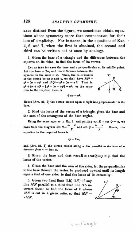
126 ANALYTIC GEOMETRY.
Y
\R U M Q
axes distinct from the figure, we sometimes obtain equa
tions whose symmetry more than compensates for their
loss of simplicity. For instance, in the equations of Exs.
4, 6, and 7, when the first is obtained, the second and
third can be written out at once by analogy.
1. Given the base of a triangle and the difference between the
squares on its sides : to find the locus of its vertex.
Let us take for axes the base and a perpendicular at its middle point.
Let the base = 2m, and the difference between the
squares on the sides = n2. Then, the co-ordinates
of the vertex being x and y, we shall have RP2 =
yi + {m + xf and PQ* = y2 + (m — xf. That is,
y2 + (m + x)1 — {y2 + (m — a:)2} = n2 ; or the equa
tion to the required locus is
4 mx — n2.
Hence (Art. 25, I) the vertex moves upon a right line perpendicular to the
base.
2. Find the locus of the vertex of a triangle, given the base and
the sum of the cotangents of the base angles.
Using the same axes as in Ex. 1, and putting cot R 4- cot Q = n, we
have from the diagram cot R — and cot Q = . Hence, they V
equation to the required locus is
ny = 2m;
and (Art. 25, I) the vertex moves along a line parallel to the base at a
distance from it ™ 2m : n.
3. Given the base and that rcot R± scotQ=p ± q, find the
locus of the vertex.
4. Given the base and the sum of the sides, let the perpendicular
to the base through the vertex be produced upward until its length
equals that of one side : to find the locus of its extremity.
5. Given two fixed lines OM, ON; if any
line MN parallel to a third fixed line OL in- /
tersect them : to find the locus of P where
MN is cut in a given ratio, so that MP =
nMN. 0i
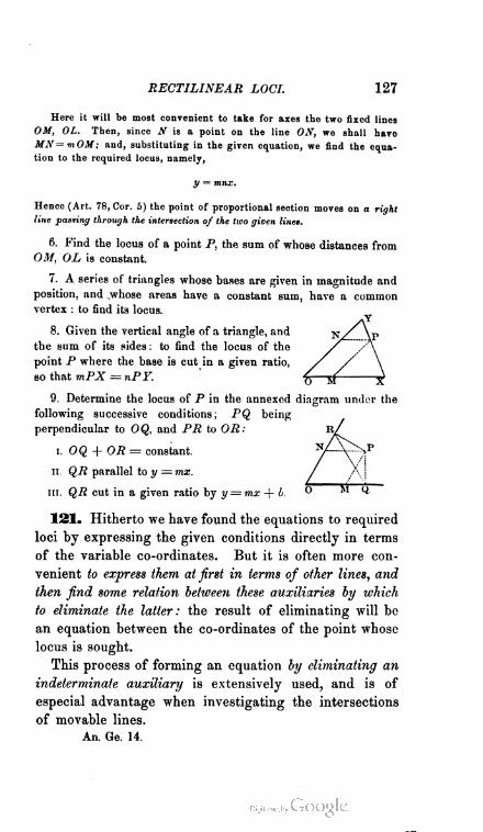
RECTILINEAR LOCI. 127
Here it will bo most convenient to take for axes the two fixed lines
OM, OL. Then, since ^ is a point on the line OX, we shall have
MX= mOM : and, substituting in the given equation, we find the equa
tion to the required locus, namely,
y = mnx.
Hence (Art. 78, Cor. 5) the point of proportional section moves on a right
fine paBting through the intersection of the two given tinea.
6. Find the locus of a point P, the sum of whose distances from
OM, OL is constant.
7. A series of triangles whose bases are given in magnitude and
position, and whose areas have a constant sum, have a common
vertex : to find its locus.
8. Given the vertical angle of a triangle, and N/_ \p
the sum of its sides : to find the locus of the / /\
point P where the base is cut in a given ratio, / / \
so that mPX = nPY. \{ ^
9. Determine the locus of P in the annexed diagram under the
following successive conditions ; PQ being
perpendicular to OQ, and PR to OR: b/
i. OQ + OR = constant. /^Y^
ii QR parallel to y = mx. / A j
in. QR cut in a given ratio by y — mx + b. ° ™ 5
121. Hitherto we have found the equations to required
loci by expressing the given conditions directly in terms
of the variable co-ordinates. But it is often more con
venient to express them at first in terms of other lines, and
then find some relation between these auxiliaries by which
to eliminate the latter: the result of eliminating will be
an equation between the co-ordinates of the point whose
locus is sought.
This process of forming an equation by eliminating an
indeterminate auxiliary is extensively used, and is of
especial advantage when investigating the intersections
of movable lines.
An. Ge. 14.
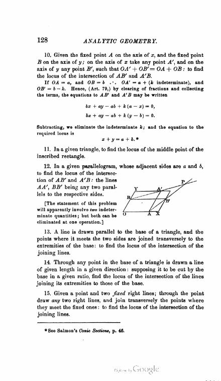
128 ANALYTIC GEOMETRY.
10. Given the fixed point A on the axis of x, and the fixed point
B on the axis of y ; on the axis of x take any point A', and on the
axis of y any point B', such that OA' + OB'= OA + OB : to find
the loeus of the intersection of AB' and A'B.
If OA = a, and OB = b . • . OA' = o + (k indeterminate), and
OB' = b — k. Hence, (Art. 79,) by clearing of fractions and collecting
the terms, the equations to AB1 and A'B may be written
6a: + ay — ab -f- k (a — x) = 0,
bx + ay — ab + k (y — b) = 0.
Subtracting, we eliminate the indeterminate k; and the equation to the
required locus is
x + y = a + b. a
11. In a given triangle, to find the locus of the middle point of the
inscribed rectangle.
12. In a given parallelogram, whose adjacent sides are a and b,
to find the locus of the intersec
tion of AB' and A'B : the lines
A A', BB' being any two paral
lels to the respective sides.
[The statement of this problem
will apparently involve two indeter
minate quantities ; but both can be
eliminated at one operation.]
13. A line is drawn parallel to the base of a triangle, and the
points where it meets the two sides are joined transversely to the
extremities of the base : to find the locus of the intersection of the
joining lines.
14. Through any point in the base of a triangle is drawn a line
of given length in a given direction : supposing it to be cut by the
base in a given ratio, find the locus of the intersection of the lines
joining its extremities to those of the base.
15. Given a point and two fixed right lines; through the point
draw any two right lines, and join transversely the points where
they meet the fixed ones : to find the locus of the intersection of the
joining lines.
*See Salmon's Conic Sections, p. 46.

PAIRS OF RIGHT LIKES. 129
122. When we have to determine the locus of the
extremity of a line drawn through a fixed point under
given conditions, it is generally convenient to employ
polar co-ordinates. We make the fixed point the pole,
and then the distance from it to the extremity of the
moving line becomes the radius vector.
16. Through a fixed point 0 is drawn a line OP, perpendicular
to a line QR which passes through the fixed
point Q : to find the locus of its extremity P,
if OP. OR = constant.
Let the distance OQ = a, and let OP.OR=mP.
From the diagram, 0R = OQ cos ROQ. Hence, the
equation to the locus of P is
pa cos 8 = m2 ;
and (Art. 82, Cor.) P moves on a right line perpendicular to OQ.
17. One vertex of an equilateral triangle is fixed, and the second
moves along a fixed right line : to find the locus of the third.
18. In a right triangle whose two sides are in a constant ratio,
one acute angle has a fixed vertex, and the vertex of the right angle
moves on a given right line: to find the locus of the remaining
vertex.
19. Given the angles of any triangle : if one vertex is fixed, and
the second moves on a given right line, to find the locus of the third.
[The student will readily perceive that Exs. 17 and 18 are particular
cases of Ex. 19. He should trace this relation through the equations to
the corresponding loci.]
20. Given the base of a triangle, and the sum of the sides;
through either extremity of the base, a perpendicular to the adjacent
side is drawn : to find the locus of its intersection with the bisector
of the vertical angle.
Section III. —Paiks of Right Lines.
123. Since the equation of the first degree always
represents a right line, there is but one locus whose equa
tion is of the first degree. But there are several loci
130 ANALYTIC GEOMETRY.
whose equations are of the second degree ; and, in accord
ance with the principle of Art. 76, we shall consider these
separately before discussing their relations to the locus
of the Second order in general. In the case of each,
we shall first obtain its equation, and then find the con
dition on which the general equation of the second degree
will represent it. When this has been done for all of
them, we can pass to the purely analytic ground, and
show that the equation of the second degree always
represents one of these lines.
We begin with the cases in which it represents a pair
of right lines. These have a special interest, as furnish
ing the title by which the Right Line takes its place in
the order of Conies.
I. GEOMETRIC POINT OF VIEW : — THE EQUATION TO A PAIR
OF RIGHT LINES IS OF THE SECOND DEGREE.
124. Any equation in the type of LMN. . . = 0 will
obviously be satisfied by supposing either of the factors
L, M, N, etc., equal to zero. If, then, L=0, M— 0,
N= 0, etc., are the equations to n different lines, their
product will be satisfied by any values of x and y that
satisfy either of them. That is, LMN. . . = 0 will be
satisfied by the co-ordinates of any point on either of the
n lines: its locus is therefore the group of lines severally
denoted by the separate factors. Hence, we form the
equation to a group of lines by multiplying together the
equations to its constituents.
125. Equation to a Pair of Bight Lines.—By
the principle just established, the required equation is
LL' = 0 ;
or, by writing the abbreviations in full, expanding, and
collecting the terms,

PAIR OF LINES THRO UGII FIXED FOIST. 131
A'A"xs+A'B"
+A"B'
y+CC'xy+B'B"y*+A'C" x+B'C"
+A"C +B"C
which is manifestly a particular case of the general equa
tion of the second degree in two variables,
Ax2 + 2Hxy + Btf + 2Gx + 2Fy + C=0,*
in which A, B, C, F, G, H are any six constants.
136. Equation to a Pair ofRight Lines passing
through a Fixed Point.—The equations to two right
lines passing through the point x'y' (Art. 101, Cor. 1)
are
A\x — x')+B' (y — 2/') - 0, A"(x — x^+B'^y—y') = 0.
Hence, (Art. 124,) the required equation is
A'A"{x-x,Y+{A'B"+A"B') {x-x') {y-y') +B'B"(y-/)'=() ;
or, since A'A", A'B"+A"B', B'B" are independent
of each other,
A(x— x'y + 2H(x -a/)(i/ -</)+-%- yj = 0.
Corollary 1.—The equation to a pair of right lines
passing through the origin (Art. 49, Cor. 3) will be
Ax2 + 2Hxy + By2 = 0.
Corollary 2.—Of the two equations last obtained, the
former is evidently homogeneous with respect to (x — x')
and (y — ?/) ; and the latter, with respect to x and y.
Hence, Every homogeneous quadratic in (x — x') and
* The equation of the second degree in two variables is usually written
Ax* + Bxy + Cy1 + Ox + Ey + F= 0.
I have followed Salmon in departing from this familiar expression. The
sequel will show, however, that the new form imparts to the equations
derived from it a simplicity and symmetry which far outweigh any incon
venience that may arise from its unfamiliar appearance.

132 ANALYTIC GEOMETRY.
(j — yO represents two right lines passing through the fixed
point x'y' ; and, Every homogeneous quadratic in x and y
represents two right lines passing through the origin.
127. The equation Ax2 + 2Hxy + By2 — 0 deserves
a fuller interpretation, as it leads to conditions which
have a most important bearing on the relations of the
Right Line to the Conies.
If we divide it by x2, it assumes the form of a complete
quadratic in y : x,
But (Arts. 124 ; 78, Cor. 5) it may also be written
(«_„)(«_.,)_. (2).
Hence, (Alg., 234, Prop. 2d,) its roots are the tangents of
the angles made with the axis of x by the two lines which
it represents. Now if we solve (1) for y : x, we obtain
y _ H±V/(H2 — AB) .
x~ B '
that is, the roots are real and unequal when H2 > AB ;
real and equal when H2 = AB ; and imaginary when
H2 < AB. Therefore, if H2 — AB> 0, the equation
denotes two real right lines passing through the origin ;
if H2—AB= 0, two coincident ones ; but in case
H2— AB<C 0, two imaginary ones.
Corollary.—The reasoning here employed is obviously
applicable to the equation of Art. 126. The meaning
of any homogeneous quadratic may therefore be deter
mined according to the following table of corresponding
analytic and geometric conditions :
ANGLE OF A PAIR OF LINES. 133
H2— AB > 0 . • . Two real right lines passing through
a fixed point.
H2 — AB= 0 . • . Two coincident right lines passing
through a fixed point.
H2—AB < 0 . • . Two imaginary right lines passing
through a fixed point.
Note—By thus admitting the conception of coincident and im
aginary lines as well as of real ones, we are enabled to assert that
every quadratic which satisfies certain conditions represents two
right lines. In fact, the result just obtained permits us to say that
every equation between plane co-ordinates denotes a line (or lines),
and to include in this statement such apparently exceptional equa
tions as
(x — af + y* = 0.
Of this equation, we saw (Art. 61, Rem.) that the only geometric
locus is the fixed point (a, 0). But it is evidently homogeneous in
(x — a), (y — 0) and fulfills the condition H* — AB<0. We
may therefore with greater analytic accuracy say that it denotes
two imaginary right lines passing through the point (a, 0) ; or, as we
shall see hereafter, two imaginary right lines whose intersection is the
center (a, 0) of an infinitely small circle.
Such statements may seem to be mere fictions of terminology;
but the farther we advance into our subject, the greater will appear
the advantage of thus making the language of geometry correspond
exactly to that of algebra. If we neglect to do so, we shall overlook
many remarkable analogies among the various loci which we in
vestigate.
128. Angle of a Pair of Right Lines.—From
Art. 96 we have, as the expression for determining this,
m! — mtan w = *—; 7 •
~ 1 + mm
But we saw (Art. 127) that m and m' are the roots of the
equation Ax2 + 2 Hxy + By2— 0. Hence,
ty(H2 — AB) , Aw! — m— -g ; mm = -g •
134 ANALYTIC GEOMETRY.
Therefore tan a = ^-r- ,— .r ^4 + i?
Corollary-—The condition that a pair of right lines shall
cut each other at right angles is
A + B = 0.
Eemark—The student can readily convince himself that when
the axes are oblique
2sinu^/(H'~AB)tan V = a i i> TTT3
A -f- B — 2 H cos u
129. Equation to the Bisectors of the angles
between the Pair Ax2 +2Hxy+ By2=0.—The equa
tion (compare Arts. 124; 109, Cor 1) will be
(A'x + B'y)2 (A"2 + B"2) — (A"x + B"yf ( An + B'2) = 0.
Expanding, collecting the terms, and dividing through by
A'B" — A"B\ this becomes
{A'B"+A"B') x1- 2 {A'A"— B'B") xy - (A'B"-Y A"B')y*= 0.
Comparing the co-efficients with those in the original
form of the equation to the two given lines (Art. 126)
we obtain
Ex1 — {A — B) xy — Hy2 = 0 .
Corollary 1.—The co-efficients of this equation satisfy
the condition (Art. 128, Cor.) A + B = 0, and show that
the two bisectors are at right angles : which agrees with
the result of Ex. 22, p. 123.
Corollary 2.—The equation to the bisectors is evidently
a quadratic in y : x of the first or second form : its roots
are therefore always real, whether those of the equation
to the given pair are real or not. Hence we have the
singular result, that a pair of imaginary lines may have
a real pair bisecting the angles between them. And it is a
noticeable inference from the discussion in Art. 127, that
two imaginary lines may have a real point of intersection.
ANAL YTIC CONDITION FOR PAIR OF LINES. 135
Remark—These two equations, Ax2 + 2Hxy + By* = 0 and
Hx*— (A — B) xy — Hy1 = 0, merit the student's special attention.
They will re-appear, in a somewhat unexpected quarter.
II. ANALYTIC POINT OF VIEW : — THE EQUATION OF THE
SECOND DEGREE ON A DETERMINATE CONDITION
REPRESENTS TWO RIGHT LINES.
130. This theorem is an immediate consequence of
the method by which we form the equation to a pair of
right lines. For, as that equation always originates in
the expression
£27= 0,
so, conversely, it must always be reducible to this form.
Hence, An equation of the second degree will represent two
right lines whenever it can be resolved into two factors of
the first degree.
Corollary.—The same reasoning manifestly applies to
LMN. . . = 0. Hence, an equation of any degree, which
can be separated into factors of lower degrees, represents
the assemblage of lines separately denoted by the several
factors. In particular, if an equation of the nth degree
is separable into n factors of the first degree, it represents
n right lines.
131. We may express the condition just determined,
in the form of a constant relation among the co-efficients
in the general equation of the second degree.
The equation to any pair of right lines may be written
{ y — (m'x + b')}{y— (m"x + b") } = 0.
Hence, (Alg., 234, Prop. 2d,) in order that the equation
of the second degree may represent two right lines, its
roots must assume the form y = mx -f- b. Now if we
solve Ax2 + 2Hxy + By2 + 2Gx + 2Fy + C= 0 as a
complete quadratic in y, we obtain
An. Ge. 1.5.
136 ANALYTIC GEOMETRY.
By=-(Hx+F)±y/{(H1-AB)x*+2(HF-BG)x+(F'—BC)\:
and in order that this may assume the form y =mx-\-b,
the expression under the radical must be a perfect square.
But the condition for this (or, in other words, the condi
tion that the general equation of the second degree may
represent two right lines) is
{H2— AB) (F2 — BC) = (HF— BGf (1).
Expanding and reducing, we may write this in the striking
symmetrical form
ABC+2FGH—AF2—BG2—CB:2 = 0 (2).
Corollary.—It is evident from (1), that H2— AB and
F2— BC will be positive together or negative together,
but will not necessarily vanish together.
133. In the light of these results, it will be interesting
to test the conditions H2— AB>0, H2— AB = 0,
H2 — AB < 0 in the general equation to a pair of right
lines.
From (1), it follows that the roots of this equation may
be written
(Hx +F)±V{(H*-AB)x*+ 2xV(H*-AB)(F*-BC) + (F?-BC)\
y— b :
hence (taking account of the preceding corollary) they
will be real and unequal, when H2 > AB; will differ by
a constant, when H2 = AB ; and will be imaginary, when
H2 < AB. But these roots are the ordinates of the two
lines represented by the equation of Art. 125 : hence, in
any equation of the second degree whose co-efficients
satisfy the condition (2), we shall have the following
criteria :
H2—AB > 0 .•. Two real, intersecting right lines.
H2—AB= 0 .•. Two parallel right lines.
H2—AB <0 .-. Two imaginary, intersecting right lines.
\
EXAMPLES ON PAIRS OF LINES. 137
Corollary.—If H2 — AB = 0, and F2 — BC=0 at
the same time, the two lines are coincident. Hence, A
right line formed by the coincidence of two others is the
limit of two parallels.
EXAMPLES.
1. Form the equation to the two lines passing through (2, 3),
(4, 5) and (1, 6), (2, 5).
2. What locus is represented by xy = 0 ? By a? — y2 = 0 ?
By ,r2 — bxy + 6/= 0? By x2 — 2xy tan 0 — y2 = 0?
3. What lines are represented by x3 — 6a:2y + llxy1 — 6y*= 0?
4. Show what loci are represented by the equations x2 -f- y2 = 0,
x2 + xy = 0, x2 + y2 + a2 = 0, a;y — or = 0.
5. Interpret (a; — a) (y — A) = 0, (a; — a)2+ (y — i)2 = 0, and
(s-y + a^ + Oe +y-a^O.
6. Show that (y — 3a; + 3) (3y + x — 9) = 0 represents two
right lines cutting each other at right angles.
7. Find the angles between the lines in Ex. 2.
8. What is the angle between the lines x2 -f- xy — 6y2 = 0?
9. Write the equation to the bisectors of the angles between
the pair x2 — bxy + 6y2 = 0.
10. Write the equations to the bisectors of the angles between
the pairs x2—y2 = 0 and x2 — xy + y2 = 0.
11. Show that the pair (>x2-\-bxy — 6y2 = 0 intersect at right
angles.
12. Show that 6a;2 + bxy — 6y2 = 0 bisect the angles between the
pair 2a;2 + 12.ry + 7y2 = 0.
13. Verify that i2 — bxy + 4y2 + x + 2y — 2 = 0 represents two
right lines, and find the lines.
14. Show that 9a;2 — I2xy + 4y2 — 2x+ y — 3 = 0 does not rep
resent right lines, and find what value must be assigned to the co-
eflicient of x in order that it may.
15. Show that 4a;2 — 12a;y + 9y2 — 4a; + 6y — 12 = 0 represents
two parallel right lines, and find the lines.
138 ANALYTIC GEOMETRY.
16. Show that 4a:2 — \2xy +V— 4a: + Oy + 1 = 0 denotes two
coincident right lines, and find the line which is their limit.
17. Show that 5a:2 — 12xy + 9j/2 — 2x + 6y + 10 = 0 represents
two imaginary right lines, and find them.
18. Show tha* if A, B, C, L, N are any five constants, the equation
to any pair of right lines may be written
(Ax + By+CY=(Lx + Nf;
that the lines are real, when (iai + iV)2 is positive; imaginary,
when (Lx + JV)2 is negative; parallel, when L = 0; and coinci
dent, when L and N are both = 0.
19. Form an equation in the type of .4a:2 + 2Hxy + By2 + 2Gx
+ 2Fy + C=0 with numerical co-eflicients, which shall represent
two real right lines.
20. Form a similar equation representing two parallel lines, and
one representing two coincident ones; also, one representing two
imaginary lines.
Section IV. —The Circle.
I. GEOMETRIC POINT OF VIEW : — THE EQUATION TO THE
CIRCLE IS OF THE SECOND DEGREE.
133. The Circle is distinguished by the following
remarkable property : The variable point of the curve is
at a constant distance from a fixed point, called the center.
134. Rectangular equation to the Circle.—If
xy represent any point on the curve, and r its constant
distance from the center gf, the required equation
(Art. 51, I, Cor. 1) will be
(x-gy + (y-fy=r*.
After expansion and reduction, this assumes the form
7? + f-2gx-2fy + (g> +f-r) = 0:
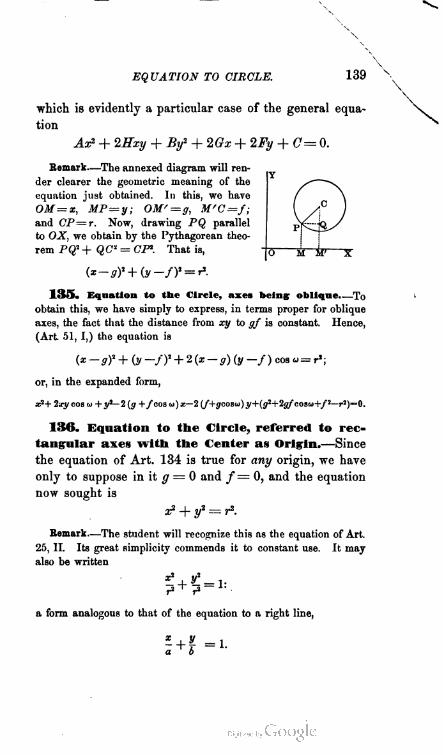
EQUATION TO CIRCLE. 139
\
which is evidently a particular case of the general equa
tion
Ax2 + 2Rxy + By2 + 2Gx + 2Fy + C= 0.
Remark—The annexed diagram will ren
der clearer the geometric meaning of the
equation just obtained. In this, we have
OM=x, MP= y; OM' = g, M'C=f;
and CP—r, Now, drawing PQ parallel
to OX, we obtain by the Pythagorean theo
rem PQ1 + QC = CP1. That is,
(*-y)* + (y -/)' = *
135. Equation to the Circle, axes being: oblique.—To
obtain this, we have simply to express, in terms proper for oblique
axes, the fact that the distance from xy to gf is constant. Hence,
(Art 51, I,) the equation is
(x - gf + (y -/)' + 2 (x - g) (y -/ ) cos o = r* ;
or, in the expanded form,
x2+ Ixy cos M + y*—2 (g +/cos u) x—2 (/+jcoso>) y+(j2+2a/'cosu+/2-''2)=0-
136. Equation to the Circle, referred to rec
tangular axes with the Center as Origin.—Since
the equation of Art. 134 is true for any origin, we have
only to suppose in it g = 0 and /= 0, and the equation
now sought is
X2 -f- y2 = r2.
Bemark—The student will recognize this as the equation of Art.
25, II. Its great simplicity commends it to constant use. It may
also be written
*
+* =
a form analogous to that of the equation to a right line,

140 ANALYTIC GEOMETRY.
137. Equation to the Circle, referred to any
Diameter and the Tangent at Its Vertex.—Since
the diameter of a circle is perpendicular to its vertical
tangent, in order to obtain the present equation we have
merely to transform the last one to parallel axes through
(— r, 0). Writing, then, x — r for x in x2 + y2 = r2, and
reducing, we find
a?+y2 — 2rx= 0;
or,
y2 = 2rx — x2.
Remark—In the equation just obtained, we suppose the origin
to be at the left-hand vertex of the diameter. It is customary to
adopt this convention. If the origin were at the right-hand vertex,
we should have to replace the x of x1 + y* = r2 by
x + r, and the equation would be Y
£2 + V1 + 2rx = 0; or, y1 — — (2 rx + a;2).
The equation of this article is verified by the 0
diagram. For (Geom., 325) MP2 = OM.MV;
that is,
y^ — x (2r — x) =2rx — x1.
The form of this equation (Art. 63) shows that the origin is on the
curve: which agrees with our hypothesis.
138. PolarEquation to the Circle.—The property
that the distance from the center (d, a) to the variable
point of the curve is constant, when expressed in polars,
(Art. 51, II) gives us
p2 + d2 — 2Pd cos (0 — a) = r2.
Hence, the equation now sought is
p2 — 2pd cos (0 — a) = 7s — d2.
Corollary 1.—Making a — 0 in the foregoing expres
sion, we obtain
p2 — 2pd cos 0 = r2 — d2 :
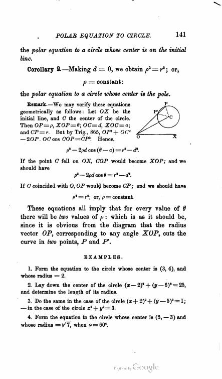
POLAR EQUATION TO CIRCLE. 141
the polar equation to a circle whose center is on the initial
line.
Corollary 2.—Making d = 0, we obtain p2 = r2 ; or,
p = constant :
the polar equation to a circle whose center is the pole.
Eemark.—We may verify these equations
geometrically as follows: Let OX be the
initial line, and C the center of the circle.
Then OP=p, XOP=6; OC=d, XOC=a;
and CP= r. But by Trig., 865, OP2 + OCl
— 2OP . OC cos COP=CP2. Hence,
p2 — 2pd cos (0 — a) = r2— d*.
If the point C fell on OX, COP would become XOP; and we
should have
p2 — 2pdcos0 = r2— d1.
If C coincided with 0, OP would become CP; and we should have
P2 = r2; or, p = constant
These equations all imply that for every value of 0
there will be two values of p : which is as it should be,
since it is obvious from the diagram that the radius
vector OP, corresponding to any angle XOP, cuts the
curve in two points, P and P' .
EXAMPLES.
1. Form the equation to the circle whose center is (3, 4), and
whose radius = 2.
2. Lay down the center of the circle (x— 2)2 + (y — 6)2 = 25,
and determine the length of its radius.
3. Do the same in the case of the circle (s+ 2)2+ (y — 5)2= 1;
— in the case of the circle x* + y2= 3.
4. Form the equation to the circle whose center is (5, — 3) and
whose radius = Yl, when « = 60°.
142 ANALYTIC GEOMETRY.
5. Form the equation to the circle whose radius = 3, and whose
center is (3, 0). Transform the equation to the opposite vertex of
the diameter.
6. Form the equation to the circle whose radius = 6, and whose
center lies, at a distance from the pole = 5, on a line which makes
with the initial line an angle = 60°.
7. Form the equation to the circle whose center is on the initial
line at a distance of 16 inches from the pole, and whose radius =
1 foot.
8. Transform the equation of Ex. 6 to rectangular axes, the origin
being coincident with the pole.
9. Form the equation to the circle whose center is at the pole,
and whose radius = 3. Transform it to rectangular axes, origin
same as pole.
10. Form the equation to an infinitely small circle whose center
is (a, 0). [Compare the result with the Remark, Art. 61, and the
Note, Art. 127.]
II. ANALYTIC POINT OF VIEW : — THE EQUATION OF THE
SECOND DEGREE ON A DETERMINATE CONDITION
REPRESENTS A CIRCLE.
139. The theorem is implied in the fact established
in Arts. 134, 135, that the equation to the Circle is a
particular case of the general equation of the second
degree. To determine the condition on which the gen
eral equation will represent a circle, we have therefore
merely to compare its co-efficients with those of the
equation to the Circle written in its most general form.
140. We saw (Art. 134) that the rectangular equation
to the Circle is
t? + f-2gx-2fy + (f +/» - r2) = 0.
Since g and / may be either positive or negative, and r
is not a function of either / or g, this may be written in
the still more general form
A(x2 + if) + 2Gx + 2Fy + C= 0.

CIRCLE AND GENERAL EQUATION. 143
If, then, the equation
Ax2 + 2Hxy + Btf + 2Gx + 2Fy + 0= 0
represent a circle, it must assume the form just obtained.
But in order to this, we must have
#=0 with A = B:
which therefore constitutes the condition that the general
equation of the second degree shall represent a circle.
Corollary.—It is obvious from the condition just deter
mined, that when the equation of the second degree
represents a circle, it also fulfills the condition
H2 — AB<0.
141. From the result of Art. 135, it follows that
H=A cos a with A = B
is the condition in oblique axes that the equation of the second degree
shall represent a circle. And it is evident that in this case, too, we
have the condition
H3— AB<0.
143. If we are given an equation in the general
form
A(x2+y2) + 2Gx + 2Fy + C= 0, ■
we can at once determine the position and magnitude of
the corresponding circle.
G2 + F2
For, by transposing C, adding —-g-— to both mem
bers, and dividing through by A, the given equation may
be thrown into the form
(.+!j+(,+;j_z±£=i?.
Comparing this with the equation of Art. 134, namely,
144 ANALYTIC GEOMETRY.
we obtain, for determining the co-ordinates of the center,
G . F .
9 =-A> f=~A'
and for determining the radius,
V(G2+F2-AC)
A
Corollary 1.—From the expressions for g and /, which
are independent of C, we learn the important principle,
that the equations to concentric circles differ only in their
constant terms.
Corollary 2.—From the expression for r, we derive the
following conclusions :
I. G2 + F2 —AC> 0 .-. the circle is real.
II. G2 + F2— AC= 0 .•. the circle is infinitely small.
III. G2 + F2— JLC< 0 .-. the circle is imaginary.
143. We may also determine the position and magni
tude of the circle by finding its intercepts on the two
axes.
Thus, if we make the y and x of the given equation
successively = 0, we obtain the two equations
Ax2 + 2Gx+O=0, Ay2 + 2Fy+ C=0.
Since each of these is a quadratic, the circle cuts each
axis in two points; and as a circle is completely deter
mined by three points, its center and radius are a fortiori
fixed by the four points thus found. We have therefore
only to find the co-ordinates of the point equidistant from
either three of the four, and we obtain the center : the
distance between this and any one of the four, is the ra
dius. Or we may proceed with greater brevity as follows :

CIRCLE TOUCHING AXES. 145
Let the intercepts on the axis of x be x1, x" ; and those
on the axis of y be y', y" : then (Alg., 234, Props. 3d
and 4th) 2G : A =— (x' + x"), 2F : A = —{y' + y"),
and C : A = x'x" ~ y'y". Hence, (Art. 142,) for deter
mining the center,
x> + x" y' + y" .
g= g ' J = 2 '
and for determining the radius,
r = i v'^+x'^ + ^ + y"2).
Corollary.—Hence, the equation to any circle whose
intercepts on the axis of x are given, is
x2 + y2— (x' + x") x — 2fy + x'x" = 0 ;
the equation to any circle whose intercepts on the axis
of y are given, is
a* + f- 2gx- (y> + y") y + y'y" = 0 ;
and the equation to the circle whose intercepts on both
axes are given, is
2 (x*+y*) — 2 (x'+x") x — 2(y'+y") y+(x'x"+y'y")=Q.
144. Of the two equations
Ax2 + 2Gx + (7= 0, ^h/2 + 2F«/ + C= 0,
the first (Alg., 237, 1) will have equal roots when
G2 = AC; and the second, when F2 — AG. Hence,
G2—AC=Q
is the condition that a circle shall touch the axis of x ;
F2—AC=0
is the condition that it shall touch the axis of y ; and
G* = F2 = AC
is the condition that it shall touch both axes.
146 ANALYTIC GEOMETRY.
EXAMPLES.
I. NOTATION AND CONDITIONS.
1. Decide whether the following equations represent circles :
Zx1 + 5xy— 7yt+2x — 4y + &=0;
hx2 — 5y2+3x — 2y + 7 = 0;
bx2 + 5y2 — 10* — 30y + 15 = 0.
2. Determine the center and radius of each of the circles
x2 + y2 + 4y — 4x — 1 = 0,
x2 + y2 + <Sx — 3y — 1 = 0.
3. Form the equation to the circle which passes through the
origin, and makes on the two axes respectively the intercepts + h
and + k.
4. Find the points in which the circle x2 + y1 = 9 intersects
the lines a; + y + 1 = 0, x + y — 1=0, and 2x + y Vb = 9.
5. What must be the inclination of the axes in order that each
of the equations
x1 — xy + y' — hx — hy = 0,
x2 + xy + y1 — hx — hy = 0,
may represent a circle ? Determine the magnitude and position
of each circle.
6. Write the equations to any three circles concentric with
2 {x1 + y1) + 6a:— 4y — 12 = 0.
7. Form the equation to the circle which makes on the axis
of x the intercepts (5, — 12), and on the axis of y the intercepts
(4, — 15). Determine the center and radius of the same.
8. What is the equation to the circle which touches the axes
at distances from the origin, each = a ?— at distances = 5 and 6
respectively ?
9. ABC is an equilateral triangle: taking A as pole, and AB
as initial line, form the polar equation to the circumscribed circle.
Transform it to rectangular axes, origin same as pole, and axis of x
as initial line.
10. If S = 0 and S/ — 0 are the equations to any two circles,
what does the equation S— k'S/=0 represent, k being arbitrary?
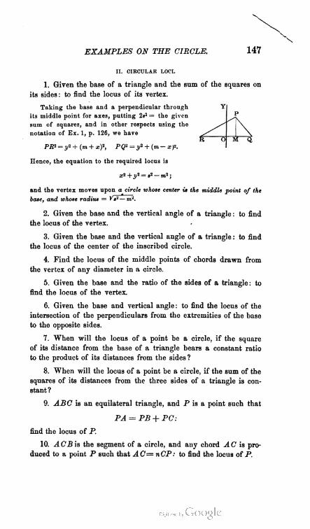
EXAMPLES ON THE CIRCLE. 147
II. CIRCULAR LOCI.
1. Given the base of a triangle and the sum of the squares on
its sides : to find the loeus of its vertex.
Taking the base and a perpendicular through
its middle point for axes, putting 2s2 = the given
sum of squares, and in other respects using the
notation of Ex. 1, p. 126, we have
PR2 = y-i + (m + xf, PQ> = y' + (m-xp.
Hence, the equation to the required locus is
X1 + y2 — ,2 _ m2 .
and the vertex moves upon a circle whose center is the middle point of the
base, and whose radius = V«2 — m2.
2. Given the base and the vertical angle of a triangle : to find
the loeus of the vertex.
3. Given the base and the vertical angle of a triangle : to find
the locus of the center of the inscribed circle.
4. Find the locus of the middle points of chords drawn from
the vertex of any diameter in a circle.
5. Given the base and the ratio of the sides of a triangle: to
find the locus of the vertex.
6. Given the base and vertical angle: to find the locus of the
intersection of the perpendiculars from the extremities of the base
to the opposite sides.
7. When will the locus of a point be a circle, if the square
of its distance from the base of a triangle bears a constant ratio
to the product of its distances from the sides ?
8. When will the locus of a point be a circle, if the sum of the
squares of its distances from the three sides of a triangle is con
stant?
9. ABC is an equilateral triangle, and P is a point such that
PA = PB + PC:
find the locus of P.
10. ACBis the segment of a circle, and any chord AC is pro
duced to a point P such that AC=nCP: to find the locus of P.
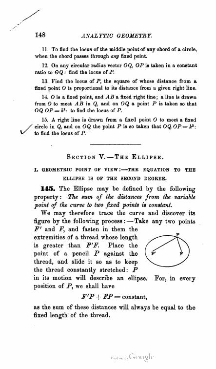
148 ANALYTIC GEOMETRY.
11. To find the locus of the middle point of any chord of a circle,
when the chord passea through any fixed point.
12. On any circular radius vector OQ, OP is taken in a constant
ratio to OQ : find the locus of P.
13. Find the locus of P, the square of whose distance from a
fixed point O is proportional to its distance from a given right line.
14. O is a fixed point, and AB a fixed right line; a line is drawn
from O to meet AB in Q, and on OQ a point P is taken so that
OQ. OP= k2 : to find the locus of P.
15. A right line is drawn from a fixed point O to meet a fixed
circle in Q, and on OQ the point P is so taken that OQ.OP= W:
to find the locus of P.
Section V. —The Ellipse.
I. GEOMETRIC POINT OP VIEW:—THE EQUATION TO THE
ELLIPSE IS OF THE SECOND DEGREE.
145. The Ellipse may be defined by the following
property : The sum of the distances from the variable
point of the curve to two fixed points is constant.
We may therefore trace the curve and discover its
figure by the following process: —Take any two points
F' and F, and fasten in them the
extremities of a thread whose length
is greater than F'F. Place the
point of a pencil P against the
thread, and slide it so as to keep
the thread constantly stretched: P
in its motion will describe an ellipse. For, in every
position of P, we shall have
F'P+FP= constant,
as the sum of these distances will always be equal to the
fixed length of the thread.

EQUATION TO ELLIPSE. 149
146. The two fixed points, F' and F, are called the
foci; and the distances with a constant sum, F'P and
FP, the focal radii of the curve.
The right line drawn through the
foci to meet the curve in A' and A,
is called the transverse axis. The A,j
point 0, taken midway between F'
and F, we may for the present call
the focal center.
The line B'B, drawn through 0 at right angles to
A'A, and terminated by the curve, is called the conjugate
axis.
147. Equation to the Ellipse, referred to its
Axes.—Let 2c = the constant distance between the foci,
and 2a — the constant sum of the focal radii.
Then, from the diagram above, F'P2 — (x + c)2 -f- y2,
and FP2 = (x — c)2 + y2. Hence, the fundamental prop
erty of the Ellipse, expressed in algebraic symbols,
will be
V{ (x + cf + y2} + V { (* - cf+ y2} = 2a.
Freeing this expression from radicals, we obtain the
required equation,
(a2 — c2) x2 + a2y2 = a2 (a2 — c2) (1) .
To abbreviate, put a2— c2 = b2, and this becomes
b2x2 + a2y2 = a2b2 (2):
which may be more symmetrically written
■ + — = 1
Remark—The student will observe the analogy between the last
form and the equation to the Right Line in terms of its intercepts.
150 ANALYTIC GEOMETRY.
148. It is important that ive should get a clear con
ception of the general form of the equation just obtained.
Let us for a moment return to the form (1),
{a2 — c2) x2 + a2y2 - a2 (a2 — c2).
In this, the definition of the Ellipse requires that a2— c2
shall have the same sign as a2 ; for the sum of the dis
tances of a point from two fixed points can not be less
than the distance between them : that is, a can not be
numerically less than c, and consequently a2 not less than
c2. Therefore, in the equation to the Ellipse, the co-effi
cients of Xs and y2 must have like signs.
Advancing now to the form (2),
b2x2 + ay= a2b2,
it is obvious that the constant term a2b2 will have but one
sign, whether the co-efficients of x2 and y2 be both positive
or both negative. Supposing, then, that a2 and b2 are both
positive, the equation after transposition would be
b2x*+ a2y2— a'b2 = 0 (3).
Supposing them both negative, it would become, after
transposition and the changing of its signs,
b2x2+ a2y2 + a2b2 = 0 (4).
Now, what is the meaning of the supposition that a2
(and thence b2) is negative ? Plainly (since in that case
we shall have, instead of a, aV— 1) it signifies that the
corresponding ellipse is imaginary.* Hence, admitting
into our conception of this curve the imaginary locus
of (4), we learn that the equation to the Ellipse is of the
general form
A'x2 + B'y2 + C = 0 :
* This interpretation is put beyond question by the form of equation
(4) itself, which denotes an impossible relation.
POLAR EQUATION TO ELLIPSE. 151
in which A' and B' are positive, and C is either positive
or negative according as the curve is imaginary or real.
149. We may at this point derive from the equation
to the Ellipse a single property of the curve, as we
shall need it in discussing the general equation of the
second degree.
Definition.—A Center of a Curve is a point which
bisects every right line drawn through it to meet the
curve.
Theorem.—In any ellipse, the focal center is the center
of the curve. The equation to any right line drawn
through the focal center (Art. 78, Cor. 5) is
y — mx.
Comparing this with the equation to any ellipse, namely,
we see that if x', y' satisfy both equations, — x', — y'
will also satisfy both. In other words, the points in
which the ellipse is cut by any right line drawn through
the focal center may be represented by x', y1 and — x',
— y. But these symbols (Art. 51, I, Cor. 2) necessarily
denote two points equidistant from the focal center:
which proves the proposition.
15©. Polar Equation to the Ellipse, the Center
being the Pole.—Replacing (Art. 57, Cor.) the x and
y of a2y2 + Vx2= a2b2 by p cos d and p sin 0, we find
P a2 sin20 + b2 cos2d '
that is, (Trig., 838,)
2_ a2b2
p a2— (a2— V) cos20 "
An. Ge. 16.
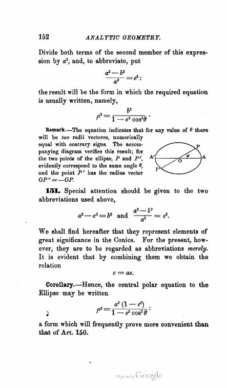
152 ANALYTIC GEOMETRY.
Divide both terms of the second member of this expres
sion by a2, and, to abbreviate, put
a2 — b2
-——=e2:a2
the result will be the form in which the required equation
is usually written, namely,
b2
p2-~l — e2 cos2(? '
Remark—The equation indicates that for any value of 0 there
will be (wo radii vectores, numerically
equal with contrary signs. The accom
panying diagram verifies this result; for
the two points of the ellipse, P and P/,
evidently correspond to the same angle 0,
and the point P' has the radius vector
OP"=—OP.
151. Special attention should be given to the two
abbreviations used above,
a2—b2
a? — c2 — b2 and ;— = e2.a'
We shall find hereafter that they represent elements of
great significance in the Conies. For the present, how
ever, they are to be regarded as abbreviations merely.
It is evident that by combining them we obtain the
relation
e = ae.
Corollary.—Hence, the central polar equation to the
Ellipse may be written
a form which will frequently prove more convenient than
that of Art. 150.
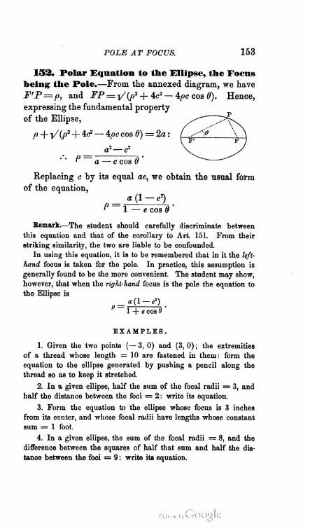
POLE AT FOCUS. 153
152. Polar Equation to the Ellipse, the Focus
being the Pole.—From the annexed diagram, we have
F'P= p, and FP=yV+ 4c2— 4pc cos d). Hence,
expressing the fundamental property
of the Ellipse,
P + V(P2 + 4c2 — 4/>c cos 6) = 2a :
a2— c2
P a — c cos 0
Replacing c by its equal ae, we obtain the usual form
of the equation,
a (1 — e2)
^ 1 — e cos d '
Remark—The student should carefully discriminate between
this equation and that of the corollary to Art. 151. From their
striking similarity, the two are liable to be confounded.
In using this equation, it is to be remembered that in it the left-
hand focus is taken for the pole. In practice, this assumption is
generally found to be the more convenient. The student may show,
however, that when the right-hand focus is the pole the equation to
the Ellipse is
P ~ 1 + e cos 6 '
EXAMPLES.
1. Given the two points (— 3, 0) and (3,0); the extremities
of a thread whose length = 10 are fastened in them: form the
equation to the ellipse generated by pushing a pencil along the
thread so as to keep it stretched.
2. In a given ellipse, half the sum of the focal radii = 3, and
half the distance between the foci = 2 : write its equation.
3. Form the equation to the ellipse whose focus is 3 inches
from its center, and whose focal radii have lengths whose constant
sum = 1 foot.
4. In a given ellipse, the sum of the focal radii = 8, and the
difference between the squares of half that sum and half the dis
tance between the foci = 9 : write its equation.

154 ANALYTIC GEOMETRY.
5. Show that in each of the ellipses hitherto given, the focal
center bisects the lines y = 2x, y = 3x, y = bx, and any others
whose equations are in the form y= mx.
6. Write the central polar equation to the ellipse in which the
difference between the squares of half the sum of the focal radii
and half the distance between the foci = 9, and the ratio of the
distance between the foci to the sum of the focal radii = 1:2.
7. Write the central polar equation to the ellipse of Ex. 2.
8. Find, in the same ellipse, the ratio of the sum of the focal
radii to the distance between the foci, and write the equation in
the form corresponding to that in the corollary to Art 151.
9. In a given ellipse, the sum of the focal radii = 12, and the
ratio between that sum and the distance from the left-hand focus
to the right-hand one = 3 : write its polar equation, the focus being
the pole.
10. The focus being the pole, form the polar equation to the
ellipse of Ex. 3. What would the equation be, if the right-hand
focus were the pole ?
II. ANALYTIC POINT OF VIEW: — THE EQUATION OF THE
SECOND DEGREE ON A DETERMINATE CONDITION
REPRESENTS AN ELLIPSE.
153. We have seen (Art. 148) that the equation to
the Ellipse may always be written in the form
A'x2 + B'tf + C = 0,
in which A' and B' are positive, and C is indeterminate
in sign. If, then, we can show that the general equation
of the second degree is reducible to this form, and can
find real conditions upon which the reduction may always
be effected, we shall have established the theorem at the
head of this article.
ELLIPSE AND GENERAL EQUATION. 155
154. In order that the general equation of the
second degree,
Ax2 + 2Bxy + By2 + 2Gx + 2Fy + C= 0,
may assume the form
A'a? + B'y2 + C = 0,
the co-efficients of its x, y, and xy must all vanish.
The question therefore is : Can we transform the equation
to axes such as will cause these co-efficients to disappear?
155. As we have seen, the equation A'x2+B'y2-\- C'—O
is referred to the center of the Ellipse, and to its axes,
which by definition cut each other at right angles. As
suming, then, as we may, that the general equation of
the second degree as above written is referred to rectan
gular axes, our first step will naturally be to determine,
if possible, the center of the locus which it represents, and
to reduce it to that center as origin.
Let x', y' be the co-ordinates of the center sought,
and let us transform
Ax2 + 2Hxy + By2 + 2Gx + 2Fy + C=0 (1)
to parallel axes passing through x'y'. Replacing (Art. 55)
the x and y of (1) by (x' + x) and (y' + y), we obtain,
after reductions,
Ax2 + 2Exy + By2 ^
+ 2 (Ax' + By' + Q) x + 2 (By'+Sx' + F) y I = 0.
+ Ax'2 + 2Hx'y' + By'2 + 2Gx' + 2Fy' +C)
Now, since this equation is referred to the center as
origin, it must (Art. 149) be satisfied equally by x, y
and — x, — y. But in order to this, we must have
Ax' + By' + G = 0, By' + Bx' + F= 0.
156 ANALYTIC GEOMETRY.
Eliminating between these simultaneous equations, we
find the co-ordinates of the center,
, BG—HF , AF—HG
x - H2 - AB ' y — IP — AB'
It is obvious that these values of x' and y' will be finite so
long, and only so long, as H2—AB is not equal to zero.
Hence we conclude that the locus of (1) has a center,
which is situated at a finite distance from the origin or
at infinity, according as (1) does not or does fulfill the
condition H2 — AB^O.
If, then, in the result of our first transformation above,
we substitute these values of x' and y', we shall obtain
an equation to the locus of (1), referred to its center.
Now the only elements of that result which depend on
x' and y', are the co-efficients of x and y, and the abso
lute term. Of these, the first two vanish, when the finite
co-ordinates of the center are substituted in them ; the
third may be thrown into the form
(Ax'+ffy'+G) x'+ (By' + Hx'+F) y'+ (Gx'+Fy'+C) :
and if in this we substitute the finite co-ordinates of the
center, it becomes
AF2 — 2FGH + BG2
H2-AB +° W5
or,
ABC+2FGB—AF2—BG2—Cff2
II2— AH ^
Hence, putting C to represent either (a) or (6), the
equation of the second degree, reduced to the geometric
center of its locus, is
Aa? + 2Hxy + By2 + <7r= 0 (2).
ELLIPSE AND GENERAL EQUATION. 157
156. The transformation from (1) to (2) has destroyed
the co-efficients of x and y, but the co-efficient of xy still
remains. Reduction to the center as origin is therefore
not sufficient to bring (1) into the form
A'xt + B'f + O'= 0.
And, in fact, we might have anticipated as much; for
the equation to the Ellipse, of which the required form
is the type, is referred not to the center merely, but to
the axes of the curve. To destroy the co-efficient of xy,
then, we must resort to additional transformation; and
our next step will naturally be to determine, if possible,
the axes of the locus represented by (2), and to revolve the
reference-axes until they coincide with them.
Let 0 = the angle made with the reference-axes of
(2) by the possible axes of the locus. Replacing (Art.
56, Cor. 3) the x and y of (2) by x cos 0 — y sin 0 and
x sin 0 + y cos 9, we obtain, after reductions,
(J.cos20 + 2#sin0cos0 + £sin20).T2 ^
— 2 { (A—B) sin 0 cos 0—ff(cos2 0—sin2 0)}xy I +C'=0 ;
+ (A sin2 0 — 2#sin 0cos0 + B cos2 0) y2 J
that is, (Trig., 847 : I, II, iv,)
%{(A+B)+ (A—B)cos20+2Ksm20}x2 ~\
—{ (A—B) sin 20—2Hcos20}xy I +C"= 0.
+ %{(A+B)— (A—B)cos20—2B7sm20}y2 J
If, in this expression, we equate to zero the co-efficient
of xy, we shall have
(A — B) sin 20 — 2Hcos 20 = 0:
2H
158 ANALYTIC GEOMETRY.
That is, since a tangent may have any value positive or
negative from 0 to oo, 2d (and therefore 0) is a real angle ;
in other words, there do exist two real lines, at right angles
to each other, which in virtue of their destroying the co
efficient of xy we may call axes of the curve to the locus
of (2). Accordingly, if in the equation last obtained we
substitute for the functions of 2d their values as implied
in (c),* the resulting equation will represent the locus,
referred to these so-called axes.
2HFrom (c), sin 26 =^{{A_Bf + {2Hy} >
cos 20 = .
V{{A-Bf + (2Hf}
Substituting these values in our last equation, we find
u(A+B)+vwfWTwy}^\
+ \ {(A + B) - V{A-By+ (2H)n f]^
whence, by writing
A' = i {(A + B) + V (A -By + {2Hf} (d),
B' = i{(A + B) — V(A—Bf + (227} («)>
the equation of the second degree, reduced to the axes of
its locus, is
AV + .By-f C"=0 (3).
*By Trig., 836, sinvl = "; cos^ = *. But since c represents the
hypotenuse, and a and b the sides, of a right triangle: c = Va* + i*.
Hence, when the tangent is given, e. g. tan A = y , we at once derive the
sine and cosine by writing
CRITERION OF THE ELLIPSE. 159
157. From (3) it appears, that, setting aside the
question of signs, the general equation of the second
degree can be reduced to the required form; provided it
is not subject to the condition H2— AB— 0.
158. It remains, then, only to inquire what condition
the general equation must fulfill in order that its reduced
form (3) may have that combination of signs which (Art.
148) is characteristic of the Ellipse.
If A' and B' are both positive, we shall have
A'B' = positive ;
or, by substituting for A' and B' from (d) and (e) above,
and reducing,
AB—H2 = positive ;
that is, changing the signs of both sides of the expression,
H2— AB = negative.
Hence, The equation of the second degree represents an
ellipse whenever its co-efficients fulfill the condition
H2— AB<0.
159. At the close of Art. 148 we saw that the sign
of C is plus or minus according as the ellipse is imag
inary or real. Let us then seek the conditions which the
general equation must fulfill in order to distinguish between
these two states of the curve.
Applying the condition H2 —AB < 0 to the value
of C as given in (b) of Art. 155, we see that, for C to
be negative, we must have
ABC+ 2FGH— AF2 — BG2 — CH2 < 0 ;
and, for C to be positive,
ABO+ 2FGff—AF2 — BG2 — QH2 > 0. '
An. Ge. 17.
160 ANALYTIC GEOMETRY.
In other words, we find that the same quantity which
(Art. 131) by vanishing indicates a pair of right lines as
the locus of the general equation, by changing sign indi
cates the transition from the real to the imaginary ellipse.
This quantity is called, in modern algebra, the Discrimi
nant of the general equation ; and we may appropriately
represent it by the Greek letter J. Adopting this nota
tion, we have
H2— AB < 0 with J<0
as the condition that the equation of the second degree shall
represent a real ellipse; and
H2— AB<0 with J>0
as the condition that it shall represent an imaginary one. *
160. We can now see, at least in part, the real bearing
of the conditions in terms of H2—AB which we some
time ago developed respecting Pairs of Right Lines.
Comparing the results of Arts. 131, 132, we infer that
H2 — AB < 0 with A = 0 (I)
is the condition that the equation of the second degree
shall represent two imaginary intersecting lines. But this
condition evidently lies between the two criteria
H2 —AB<0 with J<0 (k),
H2 — AB<0 with A > 0 (m) ;
so that we can not pass from (k) to (m) without passing
through (7). We thus learn that two imaginary right
lines intersecting each other, form the limit between the
real and the imaginary ellipse.
If we now revert to the equation (Art. 132) denoting
* In testing any given equation by these criteria, we must see that its
signs are so arranged that A (the co-efficient of x2) may be positive. The
conditions with respect to A, are derived on this assumption.
POINT AND CIRCLE AS ELLIPSE. 161
two right lines, and take its two roots separately, we see
that the two lines are
(H+ VlP—AB) x + By + {F+VF2—BC) = 0,
(H— VH'—AB) x + By + (F—VF*—BC) = 0.
Eliminating between these equations, and recollecting
[Art. 131, (1)] that
F — BO- H*_AB '
we find, as the co-ordinates of intersection for the two lines,
BG—HF AF—HG
x~ W—AB' y~H2—AB
That is, (Art. 155,) the lines intersect in the center of the
locus of the general equation. But we have seen that this
center is real, irrespective of the state of H2—AB; and
is finite, so long as H2 —AB is not zero. Hence, when
ever the equation of the second degree represents two
intersecting lines, their intersection is a finite real point,
whether they be real or imaginary.
Uniting the two conclusions thus reached, we obtain
the following important theorem : The Point, as the inter
section of two imaginary right lines, is the limiting case
of the Ellipse.
Remark,—This result is corroborated by the equation (Art. 148)
to the Ellipse itself. For if, in the expression
A'x2 + BY + C= 0,
we suppose A = 0, then C = 0 , and the equation becomes
^V + By= 0:
which (Art. 126, Cor. 2 cf. Art. 127) denotes two imaginary lines
passing through the origin ; that is, in this case, through the center.
161. The Point and the Pair of Imaginary Intersecting
Lines have thus been brought within the order of Conies.
We shall now show that the Circle likewise belongs there.
162 ANALYTIC GEOMETRY.
The condition that the equation of the second degree
shall represent a circle (Art. 140) is
LT= 0 with A = B.
But, as we noticed in the corollary to Art. 140, this is
merely a special form of the condition
H2 — AB<0.
Hence, the Circle is a particular case of the Ellipse.
Resuming, then, the equation to the Ellipse, namely,
(a2 — e2) 3? + a2y2 = a2 (a2 — e2),
we notice that it already fulfills the condition H= 0.
Adding the condition A — B, necessary to make it rep
resent a circle, we obtain, as characteristic of the Circle,
a2 — c2 — a2 .'. c = 0.
We hence learn that the Circle is an ellipse whose two
foci have become coincident at the center.
Moreover, the Circle is real, vanishes, or is imaginary,
on the same conditions as the Ellipse. For we saw
(Art. 142, Cor. 2) that it assumes these several phases
according as the quantity
G2 + F2— AC
is positive, zero, or negative. Now, if we apply to the
Discriminant A the conditions H= 0, A = B, we find,
as true for the Circle,
- A = A (G2 + F2 — AC).
And since we are always to suppose A positive, we have
J < 0 .'. a real circle.
A = 0 .•. a point.
A > 0 .*. an imaginary circle.
Eemark.—In allusion to the fact that its foci do not in general
vanish in the center, the Ellipse may be called eccentric.
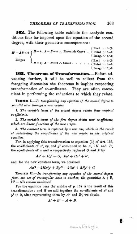
THEOREMS OF TRANSFORMATION. 163
163. The following table exhibits the analytic con
ditions thus far imposed upon the equation of the second
degree, with their geometric consequences :
f Real •■• A<0.
IP — AB<0 (H=:k> A— B = ± .-. Eccentric Curve . -J Point v A=0.
I Imag. v A>0.
ff=0,
Ellipse I f Real v A<0.
" " -.Circle J Point . . A=0
( Imag. ••• A>0.
163. Theorems of Transformation.—Before ad
vancing further, it will be well to collect from the
foregoing discussion the theorems it implies respecting
transformation of co-ordinates. They are often conve
nient in performing the reductions to which they relate.
Theorem I.—In transforming any equation of the second degree to
parallel axes through a new origin:
1. The variable terms of the second degree retain their original
co-efficients.
2. The variable terms of the first degree obtain new co-efficients,
which are linear functions of the new origin.
3. The constant term is replaced by a new one, which is the result
of substituting the co-ordinates of the new origin in the original
equation.
For, in applying this transformation to equation (1) of Art 155,
the co-efficients of x2, xy, and y1 continued to be A, 1H, and B;
the co-efficients of x and y respectively replaced Q and F by
Ax' + Hy'+G, By' + Hx' + F;
and, for the new constant term, we obtained
Ax"+ 2Hx/y/ + By'1 + 2Gx/ + 2Fy' + C.
Theorem II.—In transforming any equation of the second degree
from one set of rectangular axes to another, the quantities A + B,
H2 — AB remain unaltered.
For the equation near the middle of p. 157 is the result of this
transformation ; and if we add together the co-efficients of x2 and
y2 in it, after representing them by A' and B', we obtain
A' + B' = A + B.

164 ANALYTIC GEOMETRY.
In like manner, representing the co-efficient of xy by 2EF, and
performing the necessary operations, we find
Hn-A'B' = IP— AB.
Theorem III—If, in the process of transforming an equation of the
•second degree, the co-efficients of x and y vanish, the new origin is the
center of the locus.
For, in that event, the new equation will be satisfied equally by
x, y and — x, — y ; that is, all right lines drawn through the new-
origin to meet the curve will be bisected by that origin.
Corollary—If only one of these co-efficients vanish, the new origin
will lie on a right line passing through the center. For we must then
have either
Ax' + Hy'+ G = 0 or By' + Hx/ + F= 0 ;
that is, the co-ordinates of the new origin must satisfy one of the
equations (Art. 155) by eliminating between which we determined
the center.
Theorem IV—If the co-efficient of xy vanish, the new reference-axes,
if rectangular, will be parallel to the axes of the locus.
For when in Art. 156 * this co-efficient vanished, with the center
as origin, the new reference-axes coincided with the axes of the
locus; hence, if the origin is at any other point, they must be
parallel to them.
* As the beginner is liable to misapprehend the argument of Art. 156,
it may be well to restate it, in the form "which the present connection
suggests: — When we revolved the reference-axes through the angle
2H6=^tan-> -j^-jy,
(which was found by equating the co-efficient of xy to zero) we produced an
equation (3) identical in form with that previously obtained for the
Ellipse by referring it to its axes. So far then as concerned the Ellipse,
the new reference-axes were identical with the two lines which (Art. 146)
we had described as the axes of that curve. But on account of their
power to reduce the general equation to a fixed form, these two lines were
properly assumed to have a fixed relation to its locus, analogous to that
which they bore to tho Ellipse j and hence were called the " axes " of that
locus.
EXAMPLES ON THE ELLIPSE. 165
164. These theorems not only furnish criteria for
selecting such transformations as will represent required
geometric conditions, but they enable us to shorten the
process of transformation.
Thus, knowing Theorem I, we can henceforth write
the result of transforming to parallel axes, without going
through with the ordinary substitutions.
Knowing Theorem II, we can immediately write the
central equation of a second order curve from its general
equation, by merely setting down the first three given
terms and adding a new constant term found as in
Theorem I, 3.
By uniting Theorems II and IV, we may shorten the
process of reduction to the axes. For, if such a reduc
tion is required, we shall have H' = 0 ; and, therefore,
A' + B' = A + B with A'B'=AB— H2 : two equa
tions from which we can easily find A' and B'. C is
found as in Theorem I, 3. It is preferable, however, to
write the reduced equation at once ; for its form is
A'z? + B'y2 + C = 0 : in which A', B' are found by
formulae (d) and (e) Art. 156, arid C is obtained as
before. When the given equation is already central,
this reduction becomes very brief ; since we do not then
have to calculate C.
EXAMPLES.
I. NOTATION AND CONDITIONS.
1. Determine by inspection the locus of each of the equations
2.r2 + 3f = 12,
2.r2 + 3»/2 = 0,
2x2 + 3y2 = — 12.
2. Transform 3x* + 4.ry + y1 — bx — 6y — 3=0 to parallel axes
through (2, 3). Is the curve an ellipse?

166 ANALYTIC GEOMETRY.
3. Reduce x2 -\-2xy — ?/'-(- 8a; +4y — 8 = 0 to the center. Does
this represent an ellipse ?
4. If in a given equation of the second degree H= 0, what
condition must be fulfilled in order that the equation may represent
an ellipse ? What, if A or B equals zero ?
5. Transform 14a:* — 4ary + lly2 = 60 to the axes of the curve,
by all three methods. What is the origin in the given equation?
What is the locus, and is the same locus indicated by the reduced
equation ?
6. Find the center of 5x2 + 4xy + y1 —-5x — 2y = 19, and
reduce the equation to it. Show that the curve is a real ellipse,
both by the original equation and the reduced one.
7. Show that 14a^ — 4xy + lly2 = 0 denotes an infinitely small
ellipse ; that is, an ellipse in the limiting case.
8. Show that 5a:2 + 4xy + y* — 5x — 2y + 19 = 0 represents an
imaginary ellipse, and verify by writing the equation as referred to
the axes.
9. Find the equation to the Ellipse, the origin x'y' being on the
curve, and the reference-axes parallel to the axes of the curve.
10. Find the equation to an ellipse whose conjugate axis is equal
to the distance between its foci, taking for axes the two lines that
join the extremities of the conjugate to the left-hand focus.
II. ELLIPTIC LOCI.
1. Find the locus of the vertex of a triangle, given the base
and the product of the tangents of the base angles.
Taking the base and a perpendicular through
its middle point for axes, calling the given product Y|
P : n2, and in other respects retaining the notation
of Ex. 1, p. 126, we shall have
V Vtani?= , , tan Q = y ■
m + x m — x
V2Hence, by the conditions of the problem, mi '_ xa = —2 ; and the equation
to the required locus is
Px1 + nhj* = Pm2.
Therefore, (Art. 147) the vertex moves on an ellipse whose center is the
middle point of the haee, and whose foci are on the base at a distance from
the center = m^n2 — l2 : n.

ELLIPTIC LOCI. 167
2. Find the locus of the vertex, when the base and the sum
of the sides are given.
3 Find the loeus of the vertex, given the base and the ratio
of the sides.
4. Given the base, and the product of the tangents of the halves
of the base angles : to find the locus of the vertex.
5. Two vertices of a given triangle move along two fixed lines
which are at right angles : to find the locus of the third.
6. A right line of given length moves so that its extremities
always lie one on each of two fixed lines at right angles to each
other: to find the locus of a point which divides it in a given
ratio.
7. In a triangle of constant base, the two lines drawn through
the vertex at right angles to the sides make a constant intercept
on the line of the base : find the locus of the vertex.
8. The ordinate of any circle a? -f- /32 = r2 is moved about its
foot so as to make an oblique angle with the corresponding diam
eter : find the locus of its extremity in its new position.
9. The ordinate of any circle x2 + y2 = rJ is augmented by a
line equal in length to the corresponding abscissa: find the locus
of the point thus reached.
10. To the ordinate of any circle there is drawn a line, from
the vertex of the corresponding diameter, equal in length to the
ordinate: find the locus of the point of meeting.
11. In any ellipse, find the locus of the middle point of a focal
radius.
12. Find the locus of the extremity of an elliptic radius vector
prolonged in a constant ratio.
13. A right line is drawn through a fixed point to meet an ellipse :
find the locus of the middle point of the portion intercepted by the
curve.
14. Through the focus of an ellipse, a line is drawn, bisecting
the vectorial angle, and its length is a geometric mean of the radius
vector and the distance from the focus to the center: find the locus
of its extremity.
15. Through any point Q of an ellipse, a line is drawn parallel
to the transverse axis, and upon it QP is taken equal to the corre
sponding focal radius : find the locus of P.

168 ANALYTIC GEOMETRY.
Section VI. —The Hyperbola.
I. GEOMETRIC POINT OF VIEW:—THE EQUATION TO THE
HYPERBOLA IS OF THE SECOND DEGREE.
163. The Hyperbola is characterized by the following
property : The difference of the distances from the variable
point of the curve to two fixed points is constant.
Hence, we may trace the curve, and determine its figure,
as follows :— Take any two points, as F' and F. At F',
pivot the corner of a ruler
F'B, ; at F, fasten one end \ _^r~^f^'v-
of a thread, whose length is
less than that of the ruler.
Then, having attached the
other end to the ruler at R,
stretch the thread close against the edge of the ruler
with the point of a pencil P. Move the ruler on its
pivot, and slide the pencil along its edge so as to keep
the thread continually stretched : the path of the pencil-
point will be an hyperbola. For, in every position of P,
we shall have
F'P—FP= (F'P + PR) — (FP+ PR) =F'R—FPR.
That is, the difference of the distances from the variable
point P to the two fixed points F' and F will always be
equal to the difference between the fixed lengths of the
ruler and the thread ; or, we shall have
F'P—FP = constant.
By pivoting the ruler at F, and fastening the thread
at F', we shall obtain a second figure similar in all
respects to the former, except that it will face in the
opposite direction. The complete curve therefore con
sists of two branches, as represented in the diagram.
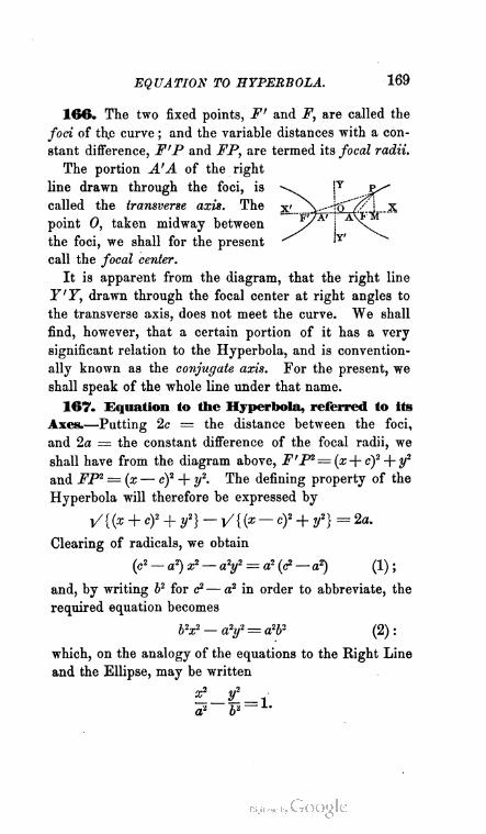
EQUATION TO HYPERBOLA. 169
166. The two fixed points, F' and F, are called the
foci of th.o curve ; and the variable distances with a con
stant difference, F'P and FP, are termed its focal radii.
The portion A'A of the right
line drawn through the foci, is -v. |Y Re
called the transverse axis. The xi j j, x-
point 0, taken midway between K/A' j
the foci, we shall for the present ~"
call the focal center.
It is apparent from the diagram, that the right line
Y'Y, drawn through the focal center at right angles to
the transverse a.xis, does not meet the curve. We shall
find, however, that a certain portion of it has a very
significant relation to the Hyperbola, and is convention
ally known as the conjugate axis. For the present, we
shall speak of the whole line under that name.
167. Equation to the Hyperbola, referred to its
Axes.—Putting 2c = the distance between the foci,
and 2a = the constant difference of the focal radii, we
shall have from the diagram above, F'P2— (x-\- cf + y2
and FP2 = (x — cf + y2. The defining property of the
Hyperbola will therefore be expressed by
V{ (x + c)2 + y2} - V{ (* - cf + y2} = 2a.
Clearing of radicals, we obtain
(c2 — a2)x2 — a2y2 = a2 (f — a2) (1);
and, by writing b2 for c2— a2 in order to abbreviate, the
required equation becomes
b2x2 — a2y2 = a2b2 (2):
which, on the analogy of the equations to the Right Line
and the Ellipse, may be written
x2 y2 v
170 ANALYTIC GEOMETRY.
Corollary.—Hence we may regard the b2 of the
Hyperbola as the negative * of the b2 of the Ellipse, and
we infer the following principle : Any function of b that
expresses a property of the Ellipse, will be converted into
one expressing a corresponding properly of the Hyperbola
by merely replacing its hbyh V—1.
Remark—The relation thus suggested between these two curves
will display itself completely when we come to discuss their prop
erties. Results will continually occur, which give color to the
fancy that an hyperbola is a reversed ellipse.
168. We must next, as in the case of the Ellipse,
investigate the general form of the equation we have
obtained.
Taking it up in the form (2), namely,
b2x* — ay = a2b2,
we speedily discover that a2 and b2 must have like signs ;
for if their signs were unlike, the equation would assume
one or the other of the forms
6V + a2f — a?b2 = 0,
b27? + a2y2 -f a2b2 = 0,
and thus would denote (Art. 148) not an hyperbola, but
an ellipse. Hence, in the equation to the Hyperbola
referred to its axes, the co-efficients of x2 and y2 must
have unlike signs.
This condition may be fulfilled either by supposing
a2 and b2 both positive or both negative. On the former
supposition, the equation will be
b2x2— a2y2— a262 = 0;
• It .must be remembered that I2 is only an abbreviation. All that is
meant, then, by the expression in the text is, that the operation for
which i>2 stands in the Hyperbola is the reverse of the corresponding one
in the Ellipse.

ITS GENERAL FORM. 171
and on the latter, after changing its signs, it will
become
b2x2 —ay + a?b2 = 0.
What, now, is the geometric meaning of the variation
in the sign of a2b2, which is thus brought into view ? In
the case of the Ellipse it indicated (Art. 148) the transi
tion from the real to the imaginary state of the curve ;
and (as the transition to + a2b2 was made by replacing
a and b by a V—1 and b V—1) we might suppose that
it indicated the same thing here, were it not that a dif
ferent conclusion is rendered certain by the following
considerations.
Let us conceive of an hyperbola whose foci F' and F
are at the same distance from their center 0 as those of
the curve already considered, but lie upon the conjugate
axis instead of the transverse.
Then, retaining the same axes of
reference as before, we shall evi
dently have, for the new positions
of F< and F,
F'F2 =x2+ (c + y)2, FP2 = x2 + (c— yf.
Supposing now that, in addition, the constant difference
of the focal radii in the new curve is 2b instead of 2a,
its equation will be
V{x2 + (c + y)2} (c-y)2} =26;
or, after clearing of radicals,
(c2 — P) */2 — b2x* = b2 (c2 — b2).
By substituting for c2— b2 its value a2, this becomes
a2y2 — bV= a2b2 ,
and, by changing the signs and transposing,
b2x2— a2f + a2b2 = Q:

172 ANALYTIC GEOMETRY.
which is precisely the expression we obtained above by
supposing, in the equation to the original hyperbola, both
a2 and b2 to be negative.
An hyperbola which thus has its foci on the conjugate
axis of another, yet at the same distance apart, and
whose a is the other's b, is said to be conjugate to the
given one. We learn, therefore, that the equation to the
Hyperbola conforms to the general type
A'x2 + B'y2 + C = 0,
in which A' is positive, B' is negative, and C is negative
or positive according as the curve is primary or con
jugate.
1G9. Theorem.—In any hyperbola, the focal center is
the center of the curve.
For the equation obtained by taking the focal center
as origin contains no variable terms except such as are
of the second degree. But (Art. 163, Th. Ill) the origin
for such an equation is the center of the curve.
17©. Polar Equation to the Hyperbola, the
Center being the Pole.—Changing b2n? — a2y2 = a2b2 to
polar co-ordinates, we find (Art. 57, Cor.)
9 b2 cos2 0 — a2 sin2 0 '
or, (Trig., 838,)
2_ a2b2
9 (a2 + b2) cos2 0 — a2 '
Dividing both terms of the second member by a2, and
putting
a2

POLAR EQUATION TO HYPERBOLA. 173
we obtain the usual form of the required equation,
namely,
b2
P2 =e2 cos2 0 — 1
Remark—Here, as well as in the case of the Ellipse, the equa
tion implies that for any value of 8 there are two radii vectores,
numerically equal, with contrary signs.
Here, too, the equation is verified by the
diagram; for the two points, P and P/,
obviously correspond to the same angle 0,
if we fix the position of P' by the radius
vector OP' = —OP.
It is also worthy of notice, that this equation may be derived
from the central polar equation to the Ellipse (Art. 150) by sub
stituting — V for 1? in the latter.
171. The two abbreviations employed above, namely,
a2 + b2
c2 — a2 = b2 and -„— = e2,
may evidently be derived from the two used in connection
with the Ellipse (Art. 151), by substituting — b2 for b2.
By combining them, however, we still obtain the relation
c — ae.
Corollary.—Hence, the central polar equation to the
Hyperbola may be written
1 — e2 cos2 6
a formula which we leave the student to distinguish
from that given for the Ellipse in the corollary to
Art. 151.
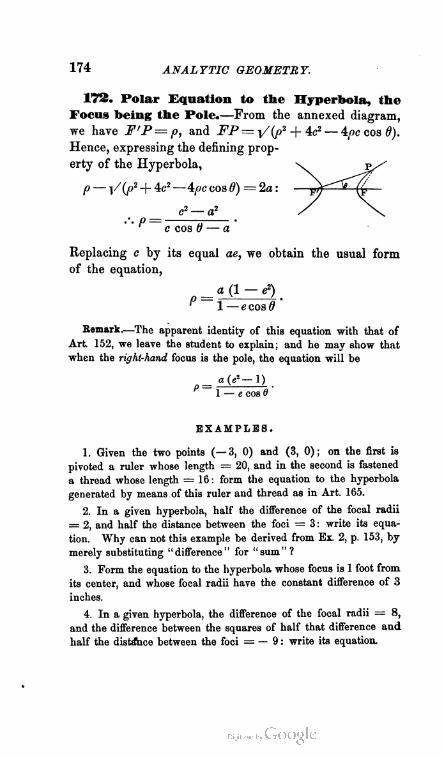
174 ANALYTIC GEOMETRY.
172. Polar Equation to the Hyperbola, the
Focus being the Pole.—From the annexed diagram,
we have F'P = p, and FP= Vip2 + 4c2 — 4/>c cos 6).
Hence, expressing the defining prop
erty of the Hyperbola, \ r>
P — V(P2 + 4«2~4,oc cos 9) = 2a :
c2 — a2
c cos 0 — a
Replacing c by its equal ae, we obtain the usual form
of the equation,
_ a (1 — e2)
P 1 — e cos 0
Remark—The apparent identity of this equation with that of
Art. 152, we leave the student to explain; and he may show that
when the right-hand focus is the pole, the equation will be
_ qQ'— 1)
1 — e cos 6
EXAMPLES.
1. Given the two points (— 3, 0) and (3, 0); on the first is
pivoted a ruler whose length = 20, and in the second is fastened
a thread whoso length = 16 : form the equation to the hyperbola
generated by means of this ruler and thread as in Art. 165.
2. In a given hyperbola, half the difference of the focal radii
= 2, and half the distance between the foci = 3 : write its equa
tion. Why can not this example be derived from Ex. 2, p. 153, by
merely substituting "difference" for "sum"?
3. Form the equation to the hyperbola whose focus is 1 foot from
its center, and whose focal radii have the constant difference of 3
inches.
4. In a given hyperbola, the difference of the focal radii = 8,
and the difference between the squares of half that difference and
half the distslhce between the foci = — 9 : write its equation.

HYPERBOLA AND GENERAL EQUATION. 175
5. Write the equations to the hyperbolas which are the conju
gates of those preceding.
6. Write the central polar equation to the hyperbola in which
the squares of half the difference of the focal radii and half the
distance between the foci differ by — 9, and the ratio of the dis
tance between the foci to the difference of the focal radii =2:1.
7. Write the central polar equation to the hyperbola of Ex. 2.
8. Find, in the same hyperbola, the ratio which the difference
of the focal radii bears to the distance between the foci, and write
the equation in the form given in the corollary to Art. 171.
9. In a given hyperbola, the difference of the focal radii = 12,
and the ratio of that difference to the distance between the foci
= 1:3. Write its polar equation, the focus being the pole.
10. The focus being the pole, form the equation to the hyperbola
of Ex. 3. What would this be, if the right-hand focus were the
pole?
H. ANALYTIC POINT OP VIEW: —THE EQUATION OP THE
SECOND DEGREE ON A DETERMINATE CONDITION
REPRESENTS AN HYPERBOLA.
173. To establish this theorem, we must show (Art.
168) that the general equation of the second degree is
reducible to the form
A'a? + By,+ C' = 0,
in which A' is positive, and B' negative ; and we must
be able to find real conditions upon which the reduction
can always be effected.
From (3) of Art. 156, we already know that, apart
from the question of signs, the general equation is re
ducible to the required form. It only remains, then, to
determine the condition which must be fulfilled in order
that the signs of A' and B' may be such as characterize
the Hyperbola.
An. Ge. 18.
176 ANALYTIC GEOMETRY.
174. If A' is positive, and B' negative, the product
A'B' must be negative. Therefore (see Art. 158) for
the Hyperbola we shall have
AB —H2 = negative ;
or, after changing the signs throughout,
H2 — AB =positive.
Hence, The equation of the second degree represents an
hyperbola whenever its co-efficients fulfill the condition
H2 -AB> 0.
175. Let us now inquire what additional criteria the
equation must satisfy, in order to distinguish between a
primary hyperbola and its conjugate.
For the reduced form of the equation, (Art. 168,) the
curve is primary or conjugate according as C is nega
tive or positive. But [Art. 155, (6)] we have
0,- fL_:v ~ H'— AB
in the case of the Hyperbola therefore, since H2 —AB
is positive, C will be negative when J is positive, and
positive when A is negative. Hence,
H2 - AB > 0 with J > 0
is the condition that the equation of the second degree
shall represent a primary hyperbola; and
H2 — AB > 0 with J < 0
is the condition that it shall represent a conjugate one.
RIGHT LINE AS HYPERBOLA. 177
176. The limit separating the two conditions just
determined, is evidently
H2— AB>0 with J = 0.
But (Arts. 131, 132 ; cf. 160) this is the condition that
the equation of the second degree shall represent two
real right lines intersecting in the center of its locus.
Hence, Two real right lines, intersecting in its center,
form the limiting case of the Hyperbola.
Remark—The student may verify this by applying the condition
A = 0 to the equation A'x1 - B'y1 + C = 0.
177. In Art. 161, we found the Circle to be a partic
ular case of the Ellipse. We shall now see that the
Hyperbola has an analogous case.
One way of satisfying the criterion of the Hyperbola
is, to have in the general equation the condition
A + B = 0.
For then H2 —AB will become H2 + A2 : which is
necessarily positive. But if A + B — 0, then (Art. 163,
Th. II) A' + B' = 0 ; and, after dividing through by A',
the equation referred to the axes will become
x2 — y2 = constant :
an expression denoting an hyperbola, by the condition
just established, and strongly resembling the equation to
the Circle,
x2 -\- y2 = constant.
Corollary.—Suppose now we push this hyperbola to its
limiting case. Its equation will of course continue to
fulfill the condition A -\- B = 0, and the corresponding
pair of right lines will therefore (Art. 128, Cor.) intersect
at right angles. Accordingly, this curve is known as the
Rectangular Hyperbola.
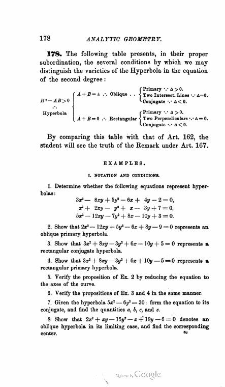
178 ANALYTIC GEOMETRY.
178. The following table presents, in their proper
subordination, the several conditions by which we may
distinguish the varieties of the Hyperbola in the equation
of the second degree :
Hyperbola
{Primary •.• A > 0.
Two Intersect. Linea v A=0.
Conjugate v A< 0.
{Primary ••• A > 0.
Two Perpendiculars ■•• A = 0.
Conjugate ••• A<0.
By comparing this table with that of Art. 162, the
student will see the truth of the Remark under Art. 167.
EXAMPLES.
I. NOTATION AND CONDITIONS.
1. Determine whether the following equations represent hyper
bolas :
3**— 8xy + by1 — 6a; + 4y — 2 = 0,
a:2 + 2xy- y2 + * - Zy + 7 = 0,
5a;2 — \2xy — 7y2 + 8x — lOy + 3 = 0.
2. Show that 2a;2 — 12a;y + 5y2 — 6x + Sy — 9 = 0 represents an
oblique primary hyperbola.
3. Show that 3a;2 + 8xy — Zy1 + 6a; — 1 Oy + 5 = 0 represents a
rectangular conjugate hyperbola.
4. Show that 3a;2 + 8xy— Zy2 + 6a; + 10y— 5 = 0 represents a
rectangular primary hyperbola.
5. Verify the proposition of Ex. 2 by reducing the equation to
the axes of the curve.
6. Verify the propositions of Ex. 3 and 4 in the same manner.
7. Given the hyperbola 5a;2 — 6y2 = 30 : form the equation to its
conjugate, and find the quantities a, b, c, and e.
8. Show that 2a:2 + xy— 15y2 — x+ 19y — 6 = 0 denotes an
oblique hyperbola in its limiting case, and find the corresponding
center.
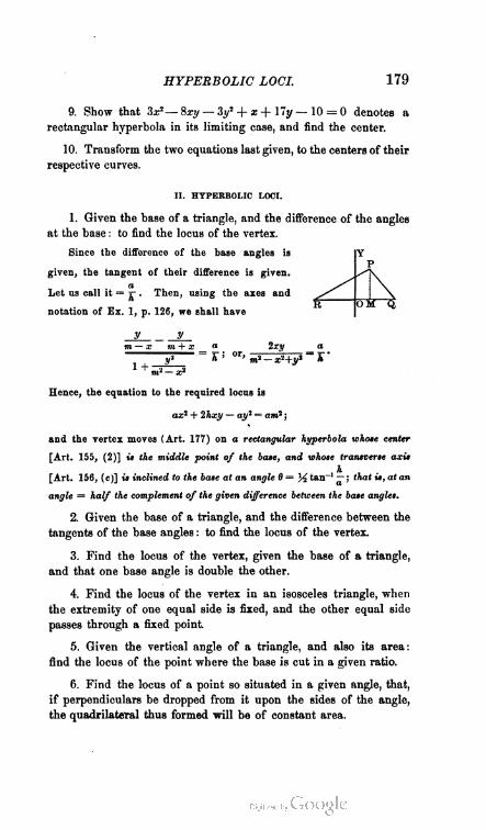
HYPERBOLIC LOCI. 179
9. Show that 3x2— Sxy — Zy1 + x + 17y — 10 = 0 denotes a
rectangular hyperbola in its limiting case, and find the center.
10. Transform the two equations last given, to the centers of their
respective curves.
II. HYPERBOLIC LOCI.
1. Given the base of a triangle, and the difference of the angles
at the base : to find the locus of the vertex.
Since the difference of the base angles is
given, the tangent of their difference is given.
aLet us call it = ^ . Then, using the axes and
notation of Ex. 1, p. 126, we shall have
Y
P
OM Q
1 + -
. ym + x _ a 2xy a
"y* A ' or' «i2 — x'+y'2 = A '
Hence, the equation to the required locus is
ax1 + Ihxy — ay1 = am' ;
and the vertex moves (Art. 177) on a reciangular hyperbola whose center
[Art. 155, (2)] is the middle point of the bate, and whose transverse axis
h[Art. 156, (c)] is inclined to the base at an angle 8= ]4 tan-1 — ; that is, at an
angle = half the complement of the given difference between the base angles.
2. Given the base of a triangle, and the difference between the
tangents of the base angles : to find the locus of the vertex.
3. Find the locus of the vertex, given the base of a triangle,
and that one base angle is double the other.
4. Find the locus of the vertex in an isosceles triangle, when
the extremity of one equal side is fixed, and the other equal side
passes through a fixed point.
5. Given the vertical angle of a triangle, and also its area:
find the locus of the point where the base is cut in a given ratio.
6. Find the locus of a point so situated in a given angle, that,
if perpendiculars be dropped from it upon the sides of the angle,
the quadrilateral thus formed will be of constant area.
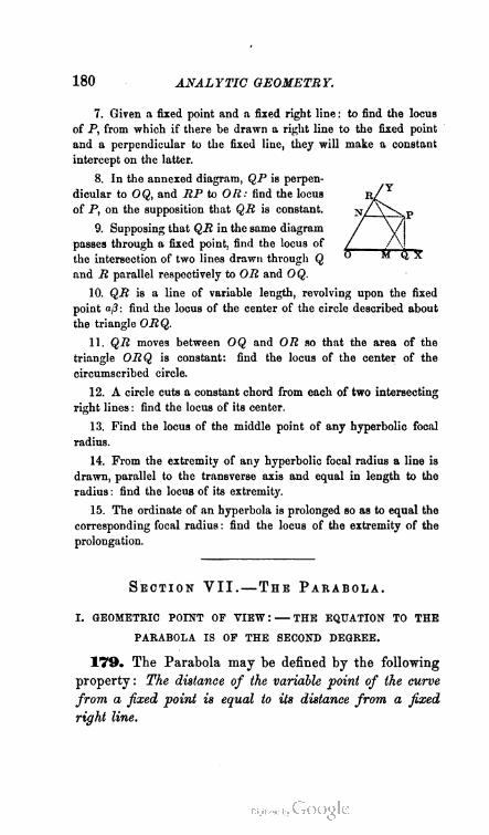
180 ANALYTIC GEOMETRY.
7. Given a fixed point and a fixed right line : to find the locus
of P, from which if there be drawn a right line to the fixed point
and a perpendicular to the fixed lino, they will make a constant
intercept on the latter.
8. In the annexed diagram, QP is perpen
dicular to OQ, and BP to OR: find the locus
of P, on the supposition that QR is constant.
9. Supposing that QR in the same diagram
passes through a fixed point, find the locus of
the intersection of two lines drawn through Q
and R parallel respectively to OR and OQ.
10. QR is a line of variable length, revolving upon the fixed
point a/3: find the locus of the center of the circle described about
the triangle ORQ.
11. QR moves between OQ and OR so that the area of the
triangle ORQ is constant: find the locus of the center of the
circumscribed circle.
12. A circle cuts a constant chord from each of two intersecting
right lines : find the locus of its center.
13. Find the locus of the middle point of any hyperbolic focal
radius.
14. From the extremity of any hyperbolic focal radius a line is
drawn, parallel to the transverse axis and equal in length to the
radius : find the locus of its extremity.
15. The ordinate of an hyperbola is prolonged so as to equal the
corresponding focal radius : find the locus of the extremity of the
prolongation.
Section VII.—The Parabola.
I. GEOMETRIC POINT OF VIEW : — THE EQUATION TO THE
PARABOLA IS OF THE SECOND DEGREE.
179. The Parabola may be defined by the following
property: The distance of the variable point of the curve
from a fixed point is equal to its distance from a fixed
right line.
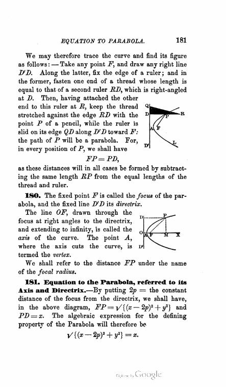
EQUATION TO PARABOLA. 181
We may therefore trace the curve and find its figure
as follows : — Take any point F, and draw any right line
D'D. Along the latter, fix the edge of a ruler ; and in
the former, fasten one end of a thread whose length is
equal to that of a second ruler RD, which is right-angled
at D. Then, having attached the other
end to this ruler at R, keep the thread Q
stretched against the edge RD with the D
point P of a pencil, while the ruler is
slid on its edge QD along D'D toward F:
the path of P will be a parabola. For,
in every position of P, we shall have
FP= PD,
as these distances will in all cases be formed by subtract
ing the same length RP from the equal lengths of the
thread and ruler.
ISO. The fixed point F is called the focus of the par
abola, and the fixed line D'D its directrix.
The line OF, drawn through the
focus at right angles to the directrix,
and extending to infinity, is called the
axis of the curve. The point A,
where the axis cuts the curve, is c
termed the vertex.
We shall refer to the distance FP under the name
of the focal radius.
181. Equation to the Parabola, referred to its
Axis and Directrix.—By putting 2p = the constant
distance of the focus from the directrix, we shall have,
in the above diagram, FP=-[/{(x — 2p)2 -\- y2} and
PD = x. The algebraic expression for the defining
property of the Parabola will therefore be
V{{x-2p)*+tf}=x.
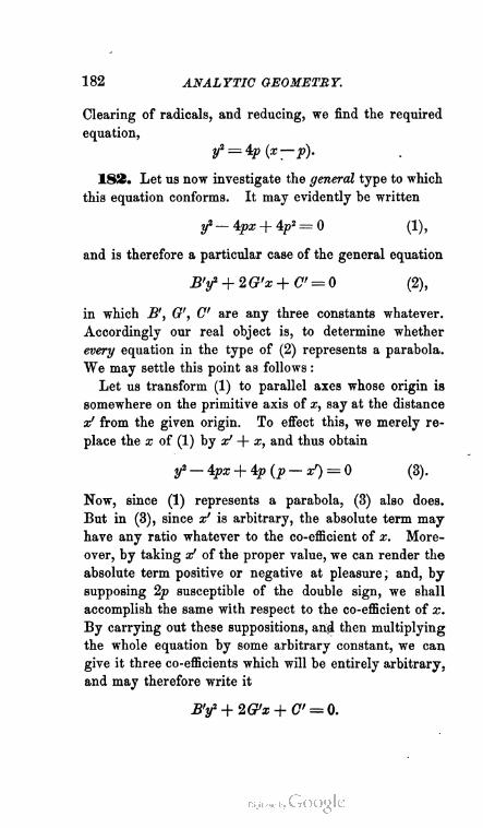
182 ANALYTIC GEOMETRY.
Clearing of radicals, and reducing, we find the required
equation,
y2 = 4p (x—p).
182. Let us now investigate the general type to which
this equation conforms. It may evidently be written
f — 4px + 4p2 = 0 (1),
and is therefore a particular case of the general equation
B'y2 + 2Q'x + C' = 0 (2),
in which B', G', C are any three constants whatever.
Accordingly our real object is, to determine whether
every equation in the type of (2) represents a parabola.
We may settle this point as follows :
Let us transform (1) to parallel axes whose origin is
somewhere on the primitive axis of x, say at the distance
x' from the given origin. To effect this, we merely re
place the x of (1) by x' + x, and thus obtain
y2 — 4px + 4p(p — x1) = 0 (3).
Now, since (1) represents a parabola, (3) also does.
But in (3), since x' is arbitrary, the absolute term may
have any ratio whatever to the co-efficient of x. More
over, by taking x' of the proper value, we can render the
absolute term positive or negative at pleasure; and, by
supposing 2p susceptible of the double sign, we shall
accomplish the same with respect to the co-efficient of x.
By carrying out these suppositions, and then multiplying
the whole equation by some arbitrary constant, we can
give it three co-efficients which will be entirely arbitrary,
and may therefore write it
B'tf + 2G'z+C' = Q.
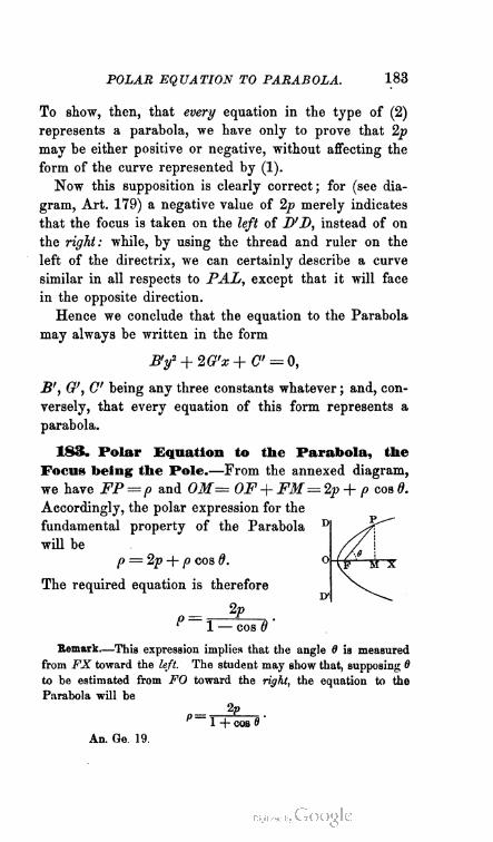
POLAR EQUATION TO PARABOLA. 183
To show, then, that every equation in the type of (2)
represents a parabola, we have only to prove that 2p
may be either positive or negative, without affecting the
form of the curve represented by (1).
Now this supposition is clearly correct ; for (see dia
gram, Art. 179) a negative value of 2p merely indicates
that the focus is taken on the left of D'D, instead of on
the right: while, by using the thread and ruler on the
left of the directrix, we can certainly describe a curve
similar in all respects to PAL, except that it will face
in the opposite direction.
Hence we conclude that the equation to the Parabola
may always be written in the form
B'f + 2G'x+ C' = 0,
B', Q', C being any three constants whatever ; and, con
versely, that every equation of this form represents a
parabola.
183. Polar Equation to the Parabola, the
Focus being the Pole.—From the annexed diagram,
we have FP= p and 0M= OF+ FM= 2p + p cos 0.
Accordingly, the polar expression for the
fundamental property of the Parabola
will be
p = 2p + p cos 0.
The required equation is therefore
2pP~l — eoad'
Remark.—This expression implies that the angle S is measured
from FX toward the left. The student may show that, supposing 6
to be estimated from FO toward the right, the equation to the
Parabola will be
2pp~l+cosf'
An. Ge. 19.

184 ANALYTIC GEOMETRY.
184. To exhibit in part the analogy of the equation
just obtained to those of the Ellipse and Hyperbola in
Arts. 152, 172, let us agree to write
e = l
as an abbreviation characteristic of the Parabola, and
analogous to those adopted in Arts. 150, 170 for the
other two curves. We may then write (see also Art. 627)
= 2p _
* 1 — ecosd
Corollary.—Adopting the convention last suggested,
we may arrange the abbreviations referred to, according
to their numerical order, thus :
Ellipse . . . . e < 1.
Parabola . . . . e = 1.
Hyperbola . . . . e > 1.
EXAMPLES.
1. Given the points (4, 0), (1, 0), (3, 0): write the rectangular
equations to the three parabolas of which they are the foci.
2. Write the rectangular equation to the parabohv whose focus is
the point ( — 3, 0).
3. Transform the equations just found to parallel axes passing
through the foci of their respective curves.
4. What are the positions of the foci with respect to the direc
trices, in the parabolas y2 = 4(x — 4), 4y' = — 3 (4x + 3), and
5y2 - 6a: + 9 = 0 ?
5. Write the focal polar equation to the parabola whose focus is
2 feet distant from the directrix, and find the length of its radius
vector when 0 = 90°. Also, find the polar equation to any parabola,
the pole being at the intersection of the axis and directrix.
PARABOLA AND GENERAL EQUATION. 185
II. ANALYTIC POINT OP VIEW : — THE EQUATION OF THE
SECOND DEGREE ON A DETERMINATE CONDITION •
REPRESENTS A PARABOLA.
185. To establish this theorem, we must show that
there are real conditions upon which the general equation
of the second degree may always be reduced to the form
(Art. 182)
B'tf + 2O'x + O' = 0.
186. In the investigation on which we are about to
enter, we must confine our attention to those equations of
the second degree whose co-efficients fulfill the condition
H2 - AB = 0.
For we have already proved (Arts. 158, 174) that
every equation of the second degree in which H2— AB
is not equal to zero, represents either an ellipse or an
hyperbola.
187. Further : The restriction just established carries
with it the additional one, that, in the equations we are
permitted to consider, the condition
J>0
can not occur.
For, reverting to the general value of the Discrimi
nant (Art. 159), we have
A = ABC+ 2FGH— AF2 — BG2 — OH2.
Whence, multiplying the second member by B : B,
adding H2F2 — H2F2 to the numerator of the result,
and factoring, we may write
. (H2-AB)(F2-BC)—{HF—BG)2
j = s

186 ANALYTIC GEOMETRY.
But, by the preceding article, we must assume
* H2 — AB = 0 ;
hence, for the purposes of the present inquiry,
{HF-BGJ
a- ^
Now the condition H2—AB= 0 obviously requires
that A and B shall have like signs ; and we have
agreed (see foot-note, p. 160) to write all our equations
so that A shall be positive: therefore B, in the present
inquiry, is positive. Whence it follows, that the fore
going expression for J is essentially negative; unless
HF— BG = 0, when it will vanish. Our proposition is
therefore established.
188. The restrictions of the two preceding articles
being accepted, our actual problem is, to determine
whether the equation
Ax2 + 2Hxy + By2 + 2Gx + 2Fy + C= 0 (1),
in which we suppose H2 — AB = 0, can be reduced to
the form
B'tf+2G'x+ C = 0;
that is, whether it can be subjected to such a transforma
tion of co-ordinates as will destroy the co-efficients of
x2, xy, and y.
189. In the first place, then, we can certainly destroy
the co-efficient of xy. For, to effect this, we need, only
revolve the axes through an angle 0, such that [Art. 156,
(c)] we may have
tan 20 = 211A—B
a condition compatible with any values of A, H, and B.

PARABOLA AND GENERAL EQUATION. 187
Making this transformation, therefore, we shall get an
equation of the form
A'x2 + B'y2 + 2G'x + 2F'y + C= 0 :
in which (see the third equation in Art. 156)
A'■= I {(A + B) + (A — B) cos 20 + 2H sin 20},
B> = } {(A + B) — (A — B) cos 20 — 2Hsm 20},
and (Art. 56, Cor. 3)
G' = G cos 0 + Fsin 0, F'=F cos 6 — G ain 0.
Now, from the value of tan 20 above, (see foot-note,
p. 158,) we know that
sin20=—tj-,— Cos2fl =
or, by applying the condition H2 = AB, and taking the
radical as negative, that
• on 2H on A-B.
and therefore, by Trig., 847, iv, and by again applying
the condition H 2 = AB, that
H B
sin0 =— ^(H'+ B2)' COsd = y^H'+ B2)
Substituting these values in the expressions for A', B',
G', and F', we obtain
j/_n- w—AA-Tt-r'— BG—HF . kv_ HG+BFA-0,B-A+B,G-^{Ht+B,y F -V{H,+Bi)
so that the proposed transformation has destroyed the
co-efficient of x2 as well as that of xy, and (1) becomes
B'y2 + 2 G'x + 2F'y +C= 0 (2).

188 ANALYTIC GEOMETRY.
190. In the second place, we can certainly destroy
the co-efficient of y. For our ability to do so depends
on finding some new origin, to which if we transform
(2) in parallel axes, the new co-efficient of y shall be
zero ; and that we can find such an origin is easily
proved. For, if the new origin be x'y', the new equation
(Art. 163, Th. I) will assume the form
B'y2 + 2G'x + 2 (B'y' +F')y + O' = 0:
in which the co-efficient of y will vanish, if
and y' being thus necessarily finite and real, while x' is
indeterminate, there is an infinite number of points,
lying on one right line, to any of which if we reduce
(2) by parallel transformation, the co-efficient of y will
disappear, and (2) will become
By + 2G'x+C' = 0 (3).
191. We see, then, that we can reduce (1) to the
required form ; and that, too, without imposing any
condition upon it other than the original one, that
H2 — AB shall be equal to zero.
Hence, The equation of the second degree will represent
a parabola whenever its co-efficients fulfill the condition
H2— AB= Q.
Corollary.—It follows from this, that whenever the
equation of the second degree denotes a parabola, its first
three terms form a perfect square.
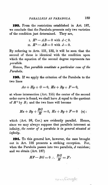
PARALLELS AS PARABOLA. 189
192. From the restriction established in Art. 187,
we conclude that the Parabola presents only two varieties
of the condition just determined. They are,
I. J5P — AB = 0 with A < 0.
II. H2—AB=0 with J = 0.
By referring to Arts. 131, 132, it will be seen that the
second of these is identical with the condition upon
which the equation of the second degree represents two
parallels.
Hence, Two parallels constitute a particular case of the
Parabola.
193. If we apply the criterion of the Parabola to the
two lines
Ax + ffy+ G = 0, Hx + By + F=0,
at whose intersection (Art. 155) the center of the second
order curve is found, we shall have A equal to the quotient
of H2 by B ; and the two lines will become
Hx + By+^= 0, L7z+By + F=0 (n):
which (Art. 98, Cor.) are evidently parallel. Hence,
since we may always suppose that parallels intersect at
infinity, the center of a parabola is in general situated at
infinity.
194. To this general law, however, the case brought
out in Art. 192 presents a striking exception. For,
when the Parabola passes into two parallels, A vanishes ;
and we obtain (Art. 187)
LTF—BG = 0 .-. BJ? = F:

190 ANALYTIC GEOMETRY.
so that, in this case, the lines in (n) become coincident,
and the center is any point on the line
Hx + By +F=0.
We thus arrive at the conception of the Right Line as
the Center of Two Parallels.
Remark—The result of this article is fully corroborated by the
equations to the two parallels themselves. For (Art. 160) these
are
Hx + By + F+ VF1 —BC= 0,
Hx + By + F— VF* — BC'= 0 :
which obviously represent two lines equally distant from
Hx + By + jP=0.
195. Two parallels, considered as a variety of the
Parabola, present three subordinate cases, each of which
has its proper criterion.
For, since the equations to the parallels are
Hx + By + F+ VF2 —BC= 0,
Hx + By + F— VF2 — BC= 0,
we shall evidently have the following series of conditions :
I. F2—BOO /. Two parallels, separate and real.
ii. F2—BC=0 .". Two coincident parallels,
in. F2—-BC<0 .•. Two parallels, separate but imaginary.
Corollary.—Hence, The Might Line, as the limit of two
parallels, is the limiting case of the Parabola.
Remark.—It is noticeable that the limit into which
the two parallels vanish when F2 — BC=0, is the line
Hx + By+F=0,

EXAMPLES ON THE PARABOLA. 191
which we have just shown to be the center of the rec
tilinear case of the Parabola.
196. The results of the foregoing articles, as fixing
the varieties of the Parabola and their corresponding
analytic conditions, may be summed up in the following
table :
A<0 .-. Center atlnfinity.
f Two Keal Parallels v F2-BC>0.
A=0.-. Center a R't Line J Single Right Line v F2—BC=0.
I Twolmag. Parallels-. •F''—BC<0.
H->-AB=Q
Parabola.
EXAMPLES.
I. NOTATION AND CONDITIONS.
1. Show why the following equations represent parabolas:
4a:2 + \2xy + V+ 6x — lOy + 5 = 0,
(2x — 5y)2 = 3x + 4y — 5,
5?/2 — 6a; + 2y — 7 = 0.
2. Show that the preceding equations represent true parabolas,
having their centers at infinity; but that
4a:2 — 12xy + V=25
denotes two parallels, whose center is the line
2x = 3y.
3. Show that 4a:2 — 12xy + 9y2 + 8x— 12y+ 5 = 0 denotes two
imaginary parallels, whose center is the real line 2a: — 3y — 2 = 0;
and that 4a;2 — 12a;y + 9y2 — 8a: + \2y + 4 = 0 denotes the limit
of these parallels.
4. Reduce 9a:2 — 24xy + 1 6y2 -f 4a: — &y — 1 = 0 to the form
BY + 2G,x+ C" = 0.
5. Show that when a parabola breaks up into two parallels, the
line Hx + By + F= 0 becomes the axis of the curve.

192 ANALYTIC GEOMETRY.
psi.— t
0-
R
II. PARABOLIC LOCI.
1. Given the base of a triangle, and the sum of the tangents
of th3 base angles: to find the locus of the vertex.
r.
Let us take the base for the axis of yt and a per
pendicular through its middle point for the axis of x.
Then, in the annexed diagram, OM will be the ordi
nate, and MP the abscissa of the variable vertex P.
Therefore, supposing the length of the base = 2m,
and the given sum of tangents = n, we shall have
— x — x
»TTy m—y '
and the equation to the locus sought will bo ny'2 — 2m.r — nm2 — 0.
Hence, (see close of Art. 182,) the vertex moves on a parabola whose axis
is the perpendicular through the middle of the base.
By comparing this equation with (3) of Art. 182, it will be seen that
the distances of the directrix and focus from the base are respectively
£(„*+ !),
2. Given the base and altitude of a triangle: to find the locus
of the intersection of perpendiculars drawn from the extremities
of the base to the opposite sides.
3. Given a fixed line parallel to the axis of a;, and a movable
line passing through the origin: to find the locus of a point on
the latter, so taken that its ordinate is always equal to the portion
of the former included between the axis of y and the moving line.
4. Lines are drawn, through the point where the axis of a par
abola meets the directrix, so as to intersect the curve in two points:
to find the locus of the points midway between the intersections.
5. Through any point Q of a circle, OQ is drawn from the
center 0, and Qli made a chord parallel to the diameter EOT and
bisected in S: to find the locus of P, where OQ and ES intersect.
6 Find the locus of the center of a circle, which passes through
a given point and touches a given right line. [Take given line for
axis of y, and its perpendicular through given point for axis of x.]
7. Given a right lino and a circle : to find the locus of the center
of a circle which touches both. [Take perpendicular to given line,
through center of given circle, for axis of z.]

LOCUS OF SECOND ORDER. 193
8. OA is a fixed right line, whose length = a; about 0, a second
line POP' revolves in such a manner that the product of the areas
PA 0, P'A 0 = a\ and their quotient = cot2 J POA : to find the
locus of P or P'. [Polars.]
9. Given the base of a triangle, and that the tangent of one base
angle is double the cotangent of half the other: to find the locus
of the vertex.
10. Find the locus of the center of a circle inscribed in a sector
of a given circle, one of the bounding radii of the sector being fixed.
Section VIII.—The Locus of the Second
Order in General.
197. We have now seen that the equations to the
Pair of Right Lines, the Circle, the Ellipse, the Hyper
bola, and the Parabola, are all of the second degree.
We have proved, too, that the general equation of the
second degree may be made to represent either of these
loci, by giving it co-efficients which fulfill the proper con
ditions ; and, in the course of the argument, it has come
to light that the Point, the Pair of Lines in their various
states of intersection, parallelism, and coincidence, and the
Circle, are phases of the three curves mentioned last.
The latter result suggests the question, Is not the gen
eral equation, considered without reference to any of these
conditions, the symbol of some locus still more generic than
either the Ellipse, the Hyperbola, or the Parabola, of which
these three curves are themselves successive phases? It is
the object of the present section, to show that this ques
tion, in a certain important sense, is to be answered in
the affirmative ; and to aid the student in forming an
exact conception of what is meant by the phrase Locus
of the Second Order in General.
194 ANALYTIC GEOMETRY.
198. We proceed, then, to show that such a locus
exists ; and to explain the peculiar nature of the existence
which belongs to it.
In the first place, a moment's reflection upon the dis
cussions in the preceding pages will convince us that
hitherto we have not regarded the equation
Ax2 + 2Hxy + By2 + 2Gx +2Fy+ C=0 (1)
in the strictly general aspect at all. For we have sup
posed its co-efficients to be subject to some one of the
three conditions
H* — AB<0, H2 —AB = 0, H2— AB>0,
and therefore to be actual numbers, since it is only in
actual numbers that the existence of such conditions can
be tested. But, obviously, we can conceive of equation
(1) as not yet subjected to any such conditions, the
constants A,B,C, F,G,H not being actual numbers, but
symbols of possible ones; and, in fact, we must so con
ceive of it, if we would take it up in pure generality.
In the second place, not only does the equation await
this purely general consideration, but when so considered
it still has geometric meaning. For, though its co-efficients
are indeterminate, its exponents are numerical and fixed :
it therefore still holds its variables under a constant law,
not so explicit as before, but certainly as real. It is still
impossible to satisfy it by the co-ordinates of points taken
at random ; it will accept only such as will combine to
form an equation of the second degree.
Since, then, we must consider (1) in its purely general
aspect as well as under special conditions ; since, even in
this aspect, it still expresses a laiv of form; and since
this law, consisting as it does in the mere fact that the

THE LOCUS AS PURE LAW.
equation is of the second degree, must pervade all the
curves of the Second order: it follows that this law
may be regarded as a generic locus, whose properties
are shared alike by the Ellipse, the Hyperbola, and
the Parabola.
109. By the phrase Locus of the Second Order in
General we therefore mean not a figure but an abstract
law of form. It exists to abstract thought, but can not
be drawn or imagined. To illustrate the nature of its
existence by a more familiar case, we may compare it to
that of the generic conception of a parallelogram. We
can define a parallelogram ; but if we attempt to imagine
or draw one, we invariably produce some particular phase
of the conception— either a rhomboid, a rhombus, a rect
angle, or a square. In the same way, the Locus of the
Second Order exists so as to be defined ; but not other
wise, except in its special phases. In short, when
speaking of it, we are dealing with a purely analytic
conception ; and the beginner should avoid supposing
that it is any thing else.
200. Further: This common lata of form not only
manifests itself in all the three curves we have been
considering, but they may be regarded as successive
phases of it, whose order is predetermined. For, as we
have seen, they may be supposed to arise out of the
general locus whenever the condition characteristic of
each is imposed on the general equation. Now these
conditions may be summed up as follows :
H2 — AB<0, H2— AB = 0, H2-AB>0.
A < 0, A = 0, A > 0.
F2—BC<Q, F2— BC = 0, F2 — BC>0.
//

196 ANALYTIC GEOMETRY.
Hence, since 0 lies between — and +, while the condi
tions in J actually entered our investigations as subordi
nates of those in H2 — AB, and the conditions in
F2 — BC as subordinates of A — 0, it follows that the
three curves have a natural order corresponding to the
analytic order of their criteria, and that their several
varieties have a similar order corresponding to theirs.
Accordingly, we should expect the curves to occur thus :
Ellipse ; Parabola ; Hyperbola. In due time hereafter,
this order will be verified geometrically.
201. Our three curves and their several varieties are
thus shown to be species of the Locus of the Second
Order : are there any others ? We shall now show that
there are not, by proving that every equation of the
second degree must represent one of the three curves
already considered.
We have just seen that all the conditions hitherto
imposed on the general equation are subordinate to the
three,
H2—AB<0, H2 — AB = 0, S2—AB>0;
and we have proved that any equation of the second
degree fulfilling either of these must represent one of the
three curves. But no equation of the second degree can
exist without being subject to one of these conditions;
for, whatever be the numerical values of A, H, and B,
we can always form the function H2 —AB, which can
not but be less than, equal to, or greater than zero.
Hence, the series of conditions already imposed on the
general equation exhaust the possible varieties of its
locus, and we have the proposition at the head of this
article.
202. We mentioned in Art. 47, that the term Conic
Section or Conic is used to describe a curve of the
THE CONIC IN GENERAL. 197
Second order. From what has now been shown, we may
define the Conic in General as the embodiment of that
general law of form which is expressed by the uncondi
tioned equation of the second degree.
It also follows that there are three species of the Conic,
corresponding to the three leading conditions which have
become so familiar.
203. Let us now recapitulate the argument by which
we have thus gradually established the theorem : —Every
equation of the second degree represents a conic.
I. We proved (Arts. 153—162) that every equation of the second
degree whose co-efficients fulfill the condition H'1 — AB < 0, repre
sents an ellipse, and showed that the Point, the Pair of Imaginary
Lines, and the Circle, are particular cases of that curve.
II. We proved (Arts. 173—178) that every equation of the second
degree whose co-efficients fulfill the condition H2— AB >0, repre
sents an hyperbola, and showed that the Pair of Real Intersecting
Lines are a case of that curve.
III. We proved (Arts. 185—196) that every equation of the second
degree whose co-efficients fulfill the condition H* — AB — 0, repre
sents a parabola, and showed that Two Parallels, whether separate,
coincident, or imaginary, are a case of that curve.
IV. We combined (Art. 200) the results of the three preceding
steps, and inferred that, of the conditions previously imposed, the three
H1— AB<0, W-AB-=0, H2 — AB>0
were all that we needed to consider in testing the leading signifi
cation of the equation of the second degree, since all the others
had proved to be subordinates of these.
V. We showed (Art. 201) that these three conditions are of such
a nature that every equation of the second degree must be subject
to one of them; and thence inferred the theorem.
204. The existence of three conditions by which the
signification of the general equation may be varied, indi
cates, as we have already noticed, three species of the
Conic. But we must not overlook a previous subdivision
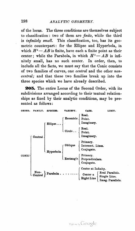
198 ANALYTIC GEOMETRY.
of the locus. The three conditions are themselves subject
to classification : two of them are finite, while the third
is infinitely small. This classification, too, has its geo
metric counterpart : for the Ellipse and Hyperbola, in
which H2 — AB is finite, have each a finite point as their
center; while the Parabola, in which H2— AB is infi
nitely small, has no such center. In order, then, to
include all the facts, we must say that the Conic consists
of two families of curves, one central and the other non-
central; and that these two families break up into the
three species which we have already described.
205. The entire Locus of the Second Order, with its
subdivisions arranged according to their mutual relation
ships as fixed by their analytic conditions, may be pre
sented as follows:
ORDER. FAMILY. SPECIES.
Ellipse .
CONIC
Central
VABIETY.
Eccentric
Non-
Central
Hyperbola
\ Parabola .
Circle .
Oblique
Keetang'r
CASE.
Real.
Point.
Imaginary.
Real.
Point.
Imaginary.
Primary.
Intersect. Lines.
Conjugate.
Primary.
Perpendiculars.
Conjugate.
f Center at Infinity.
I . f Real ParallelsCenter a
[ Right LineSingle Line.
Imag. Parallels.
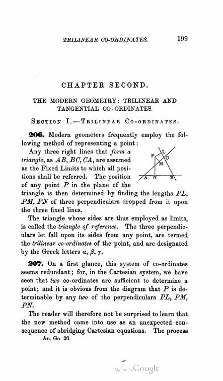
TRILINEAB CO-ORDINATES. 199
CHAPTER SECOND.
THE MODERN GEOMETRY: TRILINEAR AND
TANGENTIAL CO-ORDINATES.
Section I.—Trilinear Co-ordinates.
206. Modern geometers frequently employ the fol
lowing method of representing a point :
Any three right lines that form a
triangle, as AB, BC, OA, are assumed
as the Fixed Limits to which all posi
tions shall he referred. The position
of any point P in the plane of the
triangle is then determined by finding the lengths PL,
PM, PN of three perpendiculars dropped from it upon
the three fixed lines.
The triangle whose sides are thus employed as limits,
is called the triangle of reference. The three perpendic
ulars let fall upon its sides from any point, are termed
the trilinear co-ordinates of the point, and are designated
by the Greek letters a, /?, y.
207. On a first glance, this system of co-ordinates
seems redundant ; for, in the Cartesian system, we have
seen that two co-ordinates are sufficient to determine a
point; and it is obvious from the diagram that P is de
terminable by any two of the perpendiculars PL, PM,
PN.
The reader will therefore not be surprised to learn that
the new method came into use as an unexpected con
sequence of abridging Cartesian equations. The process
An. Ge. 20.
200 ANALYTIC GEOMETRY.
by which the trilinear system thus grows out of the
bilinear, will now be explained.
208. In Art. 108, we have already hinted at the
Abridged Notation, which gives rise to the system of
which we are speaking. We will now present the subject
in detail.
If the equation to any right line is written in terms of
the direction-cosines of the line, namely, in the form
x cos « + y sin a —p = 0,
we may use a as a convenient abbreviation for the whole
member equated to zero ; for it naturally recalls the ex
pression into which it enters as so prominent a constant.
Similarly, in the equations
x cos $ + y sin /9 —p' — 0,
x cos y + y sin y —p" = 0,
we may represent the first members by ft and y- Thus
the equations to any three right lines may be written
a = 0, /9 = 0, y = 0.
The brevity of these expressions is advantageous, even
when they are taken separately ; but it is not until we
combine them, that the chief value of the abridgment
appears. We then find that it enables us to express, by
simple and manageable symbols, any line of a given
figure in terms of three others.
209. It is this last named fact, which constitutes the
fundamental principle of trilinear co-ordinates. That we
can so express a line, follows from our being able (see
Art. 108) to write, in terms of the equations to two given
right lines, the equation to any line passing through their
intersection.
ABRIDGED NOTATION. 201
210. We may convince ourselves of this, by a few
simple examples. If a = 0, /9 = 0 represent any two
right lines, then (Art. 108)
a + kp = 0
is the equation to any right line passing through their
intersection, provided h is indeterminate. Now k, in
this equation, (Art. 108, Cor. 2) is the negative of the
ratio of the perpendiculars dropped from any point in
the line a + hp = 0 upon the two lines a — 0 and /? = 0.
Therefore, writing k so as to display its intrinsic sign,
a + k[$ = 0
denotes a right line passing through the intersection of
a — 0 and /9 = 0, and lying in that angle of the .two
lines which is external to the origin ; but
a— 7c/? = 0
denotes one lying in the same angle as the origin.
Moreover, when the perpendiculars mentioned are equal,
the value of h= ± 1 ; and we have (Art. 109, Cor. 3)
« + /9 = 0
the equation to the bisector of the external angle between
two given lines, and
a — p = 0
the equation to the bisector of the infernal angle.
Suppose, then, that we have a given triangle, whose
sides are the three lines
a = o, p = 0, y = o.
Granting, as we may, that the origin is within the triangle,
the equations to the three bisectors of the angles will be
a — 0 = 0, ft — r = 0, y — a = 0.
202 ANALYTIC GEOMETRY.
The equations to the three lines which bisect the three
external angles of the triangle, will be
« + /9 = 0, /3+r = 0, r + «-o.
Thus, these six lines of the triangle are all expressed in
terms of its three sides.
311. We can of course extend this system of abbre
viations to the case of lines whose equations are in the
general form
Ax+By + C=Q,
by representing the member equated to zero by a single
English letter, such as L or v. Thus,
L + kL' = 0 or v + kv' = 0
denotes a line passing through the intersection of the
lines
Ax + By + O=0, A'x + B'y + C = 0.
It must be borne in mind, however, that in these equa
tions k does not denote the negative of the ratio of the
perpendiculars mentioned above, and in consequence
does not become ± 1 when those perpendiculars become
equal. Hence, in these cases, the equations to the ex
ternal and internal bisectors of the angle between two
given lines, are respectively (see Art. 109, Cor. 4)
L + rL' =0 or Iv + mv' = 0,
L — rL' =0 or Iv — mv' = 0,
in which r, or m : I, is to be determined by the formula on
p. 116.
In this notation, if the three sides of a triangle are
tt=0, v — 0, w—0,
ABRIDGED NOTATION. 203
the three bisectors of its interior angles may be repre
sented by
lu —m»= 0, mv — nw = 0, nw — lu = 0 ;
and the three bisectors of its exterior angles, by
lu + mv = 0, mv + nw = 0, nw + lu = 0.
Here, too, the six lines are all expressed in terms of the
three sides.
212. Having thus learned how to interpret the equa
tions
a ± /9 = 0, /3±r = 0, r±a = 0
when a=0, /3 = 0, f = 0 are given as forming a tri
angle, we next advance to the interpretation of
la + mj3 -\- ny = 0:
an equation of which the preceding six are evidently
particular cases, and in which I,- m, n are any three
constants whatever.
On the surface, this looks like the condition (Art. 114)
that the three lines a = 0, /? = 0, f=0 shall meet in
one point* But the terms of that condition are, that
three lines will meet in one point whenever three con
stants can be found such that, if the equations to the lines
he each multiplied by one of them, the sum of the products
will be zero. Hence, the I, m, and n of that condition are
not absolutely arbitrary, but only arbitrary within the
limits consistent with causing the function la -f- mfl + ny
to vanish identically. On the contrary, the I, m, and n
of the present equation are absolutely arbitrary.
With this fact premised, let us now investigate the
meaning of the equation.

204 ANALYTIC GEOMETRY.
213. If we replace «, ft, and y by the functions for
which they stand, and reduce the equation on the sup
position that x and y have but one signification in all
its three branches, we obtain
(I cos a + m cos ft + n cos y) x
+ (I sin a + m sin ft + n sin 7-) «/
+ /p + Wip' + Tip"
which is evidently the equation to some right line, since
it conforms to the type
Ax + By+ C=0.
Its full significance, however, will not appear until we
discuss it under each of three hypotheses concerning the
relative position of the three lines whose equations enter
it. To this discussion, we devote the next three articles.
214. Let the three lines a — 0, ft = 0, y = 0 meet in
one point.
When this is the case, the equation
la + mft + ny — 0
denotes a right line passing through the point of triple
intersection. For the co-ordinates of this point will
render a, ft, and y equal to zero simultaneously, and
will therefore satisfy the equation just written.
215. Let the three given lines be parallel.
In this case, their equations (Art. 98, Cor.) may be
written
a = 0, a + c' = 0, a + c" = 0,
and the equation we are discussing will thus become
(I + m + n) a + (mo' + nc") = 0 ;
that is, it will assume the form
« + c = 0,

a, ft, y, AS CO-ORDINATES. 205
and will therefore denote a right line parallel to the three
given ones.
216. Let the three given lines form a triangle.
In this case the preceding results are avoided; hence,
the equation of Art. 213 assumes the form
Ax + By + C=0
without imposing any restriction upon the values of A,
B, and C. In this case, therefore, it denotes any right
line whatever.
This result is simply the extension of that obtained in
Arts. 210, 211 ; and shows that we can (as was stated
in Art. 208) express any line of a figure in terms of three
given ones.
217. From the results of the last three articles, we
conclude that
la + m,p -f- ny = 0
is the equation to any right line ; provided, however,
that the lines
a = 0, p=0, y = 0
are so situated as to form a triangle. This proviso, we
can not too carefully remember.
218. The examination of an example somewhat more
complex than any yet presented, will convince us that
this abridged method of writing equations is in effect a
new system of co-ordinates, applicable to lines of any order.
Before commencing this example, it may be necessary
to remind the student that the use of a Greek letter for
an abbreviation, always implies that the equation to the
line so represented is in the form
x cos a + y sin a — p = 0,
and the like ; and that, when the fundamental equations

206 ANALYTIC GEOMETRY.
are in any other form, they will be abridged by means of
English characters.
For the sake of still greater brevity, the line a = 0 is
often cited as the line a, the line /3=0 as the line /3, etc.
The point of intersection of two lines is frequently spoken
of as the point aft, etc. The last notation should be care
fully distinguished from that of the co-ordinates of the same
point.
219. Example.—Any line of a quadrilateral in terms
of any three.
Let ABEF be any quadrilateral, and
let
a = 0, /? = o, r = o
be the equations to its three sides BC,
CA, AB. We can now represent any
other line in the figure, in terms of a, /?,
and y.
Suppose the origin of bilinear co-ordinates to be within the tri
angle ABC, and, in fact, within the triangle EOB. The equation
to AE, which passes through the intersection of /? and y, and lies
in their internal angle, will be of the form
m/? — ny=0 (AE).
The equation to BF, which passes through the intersection of y
and a, and lies in their internal angle, will be of the form
ny—la = Q (BF).
The equation to EF, which joins the intersections of (a, AE) and
(/3, BF), and lies in the external angle of the first two lines, but in the
internal angle of the second pair, must be formed (Art. 108, Cor. 2)
so as to equal either the sum of la and m/3 — ny or the difference
of m/? and ny— la. It is therefore
la + mp— ny = 0 (EF).
The equation to CD, which joins a/3 to the intersection of (y, EF),
and lies in the external angle of both pairs of lines, must be the
sum of either la and m/3, or ny and la + m/3 — ny. Consequently,
it is
la + m/3 = 0 (CD).

a, ft, y, AS CO-ORDINATES. 207
The equation to OC, which joins a/3 to the intersection of (AE, BF),
and lies in the internal angle of a/3, but in the external angle of the
other two lines, must be equal either to the difference of la and m/3
or the sum of m/3 — ny and ny— la. Accordingly, it is
fa-m/3 = 0 (OC).
Finally, the equation to OD, which joins the intersection of (y, EF)
to that of {AE, BF), and lies in the internal angle of both pairs
of lines, must be formed so as to equal the difference of either
la + m/3 — ny and ny, or m/3 — ny and ny — la. Therefore, it is
fa + m/3 — 2ny = 0 ( OD).
We have thus expressed all the lines of the quadrilateral in
terms of the three lines a, /?, and y. We can do more : we can
solve problems involving the properties of the figure, by means
of these equations, and test the relative positions of its lines
without any direct reference to the x and y which the symbols a,
fS, y conceal. Thus, the form of the equations
la — m/3 = 0, m/3 — ny = 0, ny — la = 0
shows (Art. 114) that the three lines OC, AE, BF meet in one
point, and the same relation between OD, AE, BF is shown in
the form of their equations.
220. We see, then, that by introducing this abridged
notation we can replace the Cartesian equations in x and
y by a set of equations in a, /9, y. Moreover, it is notice
able that all these abridged equations to right lines are
of the first degree with respect to «, /9, and y. Since,
therefore, we operate upon these symbols (as the last
example shows) just as if they were variables, and since
they combine in equations which satisfy the condition
that an equation to a right line must be of the first
degree, it appears that we may use a, /?, y as co-ordinates.
Thus, we may say that the equation
la -f- ot/9 + ny = 0
is the equation to any right line, and that a, /?, y are the
co-ordinates of any point in the line.
An. Ge. 21.

208 ANALYTIC GEOMETRY.
What now is the system of reference to which these
co-ordinates belong? We have seen that, in order to the
interpretation we have given of the last-named equation,
the lines a, ft, y must form a triangle. We know, too,
(Art. 105) that a is the length- of a perpendicular let
fall from any point to the line a ; that ft is the length
of a perpendicular from the same point to the line ft;
and that y is the length of a perpendicular from the
same point to the line y. Hence, we see that if a, ft, y
are taken as co-ordinates, they are referred to the tri
angle formed by
« = 0, ft = 0, y = 0,
and that they signify the three perpendiculars dropped
from any point in its plane upon its three sides. In
short, we have come out upon the system of trilinear
co-ordinates described in Art. 206.
PECULIAR NATURE OF TRILINEAR CO-ORDINATES.
221. Before making any further application of the
new system, it is important to notice that trilinear co
ordinates are in one respect essentially different from
bilinear. In the Cartesian system, the x and y are
independent of each other, unless connected by the
equation to some locus. In the trilinear system, on the
contrary, the a, ft, and y are each of them determined
by the other two ; that is, there is a certain equation
between them, which holds true in all cases, whether the
point which they represent be restricted to a locus or not.
In the language of analysis, we express this peculiarity
by saying that each of these co-ordinates is a determined
function of the other two.
That trilinear co-ordinates are subject to such a con
dition, is proved by the fact, that two co-ordinates com
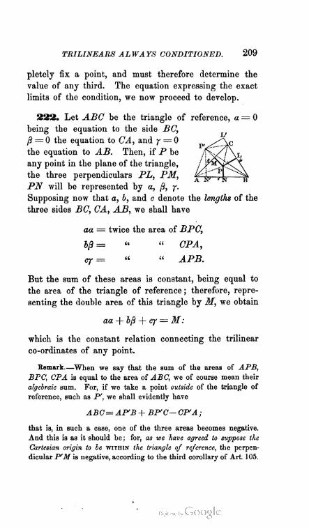
TRILINEARS ALWAYS CONDITIONED. 209
pletely fix a point, and must therefore determine the
value of any third. The equation expressing the exact
limits of the condition, we now proceed to develop.
222. Let ABC be the triangle of reference, a — 0
being the equation to the side BC,
j8 = 0 the equation to CA, and y — 0
the equation to AB. Then, if P be
any point in the plane of the triangle,
the three perpendiculars PL, PM,
PN will be represented by a, /?, y.
Supposing now that a, b, and c denote the lengths of the
three sides BO, CA, AB, we shall have
twice the area of BPC,
" " CPA,
" " APB.
But the sum of these areas is constant, being equal to
the area of the triangle of reference ; therefore, repre
senting the double area of this triangle by M, we obtain
aa + bp + cy = M:
which is the constant relation connecting the trilinear
co-ordinates of any point.
Bemark—When we say that the sum of the areas of APB,
BPC, CPA is equal to the area of ABC, we of course mean their
algebraic sum. For, if we take a point outside of the triangle of
reference, such as P', we shall evidently have
ABC= AP'B + BP'C— CP'A ;
that is, in such a case, one of the three areas becomes negative.
And this is as it should be ; for, as we have agreed to suppose the
Cartesian origin to be within the triangle of reference, the perpen
dicular P'M is negative, according to the third corollary of Art. 105.
aa =
6/3 =
cy =
210 ANALYTIC GEOMETRY.
223. This peculiarity of trilinear co-ordinates may
be made to promote the advantages of the system.
In the first place, it gives rise to a very symmetrical
expression for an arbitrary constant. For if k be arbi
trary, kM will also be; and we shall have, for the
symbol alluded to,
k (aa + 6/9 + ef) (1).
We can also modify this symbol, and render it still
more useful. Let 1 : r = the ratio of the side a, in
the triangle of reference, to the sine of the opposite
angle A. Then, by Trig., 867, we shall have
sin A sin B sin 0
— —j— = = r.a o c
Now, by the principle of Art. 222,
r (aa + bft + cy) ~ constant ;
hence, substituting for ra, rb, re from the equal ratios
above,
a sin A + /9 sin B + y sin 0= constant ;
or, the symbol for an arbitrary constant may be written
k(asinA + fismB+ysmC) (2).
224. In the second place, the peculiarity of trilinears
enables us to use homogeneous equations in all cases.
For, if a given trilinear equation is not homogeneous,
we can at once render it so by means of the relation in
Art. 222. Thus, if the given equation were ft=p, we
might write
Mp=p(aa+bfi + cy).
225. In the third place, instead of the actual trilinear
co-ordinates of a point, we may employ any three quan
tities that are in the same ratio, without affecting the
TRANSFORMATION TO BILINEARS. 211
equation to the locus of the point. For, since all tri-
linear equations are homogeneous, the effect of replacing
a, /?, y by pa, pft, py will only be to multiply the given
equation by the constant p : which of course leaves it
essentially unchanged.
This principle will often prove of great convenience.
Remark—In case it becomes desirable to find the actual tri-
linear co-ordinates when they have been displaced in the manner
described, we may proceed as follows : — Let I, m, n be the three
quantities in a constant ratio to a, /?, y: then, supposing the ratio
to be 1 : r,
a — rl, j} = rm, y — rn.
Hence, (Art. 222,)
r {la + mb + nc) = M:
from which r is readily found.
326. Finally, the property in question enables us to
pass from trilinear co-ordinates to Cartesian. For, by
means of the relation aa-\-bft-\- <:y =M, we can convert
any trilinear equation into one which shall contain only
/3 and y. Then, supposing the side y of the triangle of
reference to be the axis of x, and the side /? the axis of y,
we shall have
/? = x sin A, y = y sin A.
Corollary.—If the triangle of reference should be right-
angled at A, the reduction-formulae will become
P = x, y = y.
But, in general, to pass from trilinears to rectangulars
when the side y is taken for the axis of x, we must use
;3 = x sin A — y cos A, y = y-
The student may draw a diagram, and verify the last
formulae.
212 ANALYTIC GEOMETRY.
227. The advantage of the trilinear system consists
in this : Its equations may all be referred to three of
the most prominent lines in the figure to which they
belong, and hence become shorter and more expressive
than those of the Cartesian system, which can go no
farther in the process of simplification than the use of
two prominent lines. The student will see a good illus
tration of this in the equations to the bisectors of the
internal angles of a triangle. The trilinear equations
are
a — £ = 0, /3 — r = 0, r— a = 0
which are much simpler than the Cartesian ones given
in Ex. 32, p. 124.
TRILINEAR EQUATIONS IN DETAIL.
228. Equation to any Right Line.—This we have
already (Arts. 212—217) found to be
la + m/9 + ny = 0.
229. Equation to a right line parallel to a given
one.—It is obvious geometrically, that the «, /?, y of the
parallel line will each diner from the a, /?, y of the given
one by some constant. Hence, the given line being
la -\* mft + ny — 0, the required equation [Art. 223, (2)]
will be
la + 7W/9 + n-y -f- k (a sin A -f /? sin B + y sin C) = 0.
230. Equation to a right line situated at in
finity.—The Cartesian equation to this is 0=0, in
which (Art. 110) C is a finite constant. Therefore
(Art. 223) the trilinear equation is
a sin A + /3 siji B + y sin C= 0.

TRILINEAB EQUATIONS. 213
231. Condition that two right lines shall be
mutually perpendicular.—Let the two lines be
la + mft + ny = 0, I'a + m'ft + n'y = 0.
By writing a, ft, y in full, collecting the terms, and apply
ing (Art. 96, Cor. 3) the criterion AA' + BB' = 0, we
obtain, as the required condition,
( (mn' + m'n) cos (ft — y) \
W +mm' -f nn' + < (nV + n't) cos (y — a) f = 0
I (lm' + I'm) cos (a — ft) )
Now, in this expression, a, ft, f are the angles made with
the axis of x by perpendiculars
from the origin on the lines a, ft, y.
Supposing the latter to form the
triangle of reference, and to inclose
the origin, it is evident from the
diagram, that ft — y is the angle
between the perpendiculars ft and
y ; that ; a is the angle between
the perpendiculars y and a ; and that a — ft is the angle
between the perpendiculars a and ft. From the proper
ties of a quadrilateral it then follows, that ft — y is the
supplement of A, y — a of B, and a — ft of C. Hence,
the required condition may be otherwise written
[ {mn' + m'n) cos A
U' + mm' + nn'— < (nV + n't) cos B J- = 0.
[ (lm' -f l'm) cos C
Corollary.—The condition that la + mft + ny= 0 shall
be perpendicular to y = 0, is
w = m cos .4 + Z cos 5.

214 ANALYTIC GEOMETRY.
2152. Length of a perpendicular from any
point to a given right line.—Let the point be afty,
and the line la -f- mft + ny — 0. Write the latter equa
tion in full, collect its terms, and apply the formula of
Art. 105, Cor. 2. We thus find
la + w,9 + ny _
V\l2+m2+n-—2mn cosA—2nl cosB—2lm cos 6")
233. Equation to a right line passing through
Two Fixed Points.—The form of this will of course
be
la + 7)1)3 + ny = 0 ;
and our problem is, to determine the ratios l:m:n so
that the line shall pass through the two points a${(x,
Since the two poin-ts are to be on the line, we shall
have
lax + m/?! + nyj = 0,
la2 + mfi2 + ny2 = 0.
Solving for I : n and m : n between these conditions, we
find
I : m: n = (frfr— T&) ■ (n«2 — <*ih) : —
The required equation is therefore
« (fix* — r&) + P (n«2 — «ir2) + r ia& — = o.
Corollary.—Hence, in trilinears, the condition that
three points shall lie on one right line is
«s ii^r-i — r&) + A (ri«2 — «ir2) + r3 — ft«2) = o.
Expanding, and re-collecting the terms, we may write
this more symmetrically (see Art. 112),
«i (&rs — rA) + «2 (An — tWO + «a Oto— rA) = °-

TRILINEAR EQUATIONS. 215
234. Theorem.—Evert/ trilinear equation of the second
degree represents a conic.
For, since a, /?, y are linear functions of x and y,
every such equation is reducible to an equation of the
second degree in x and y. But the latter (Art. 203)
will represent a conic.
Remark.—In passing now to the trilinear expressions
for curves of the Second order, we shall at first suppose
the triangle of reference to have a special position, such
as will tend to simplify the resulting equations. The more
general equations, corresponding to any position of the
triangle, will be investigated afterward.
235. Equation to the Conic, referred to the
Inscribed Triangle.—To obtain this, we must form
an equation of the second degree in a, ft, y, such as the
co-ordinates of the vertices of the reference-triangle will
satisfy.
Now, at the vertex A, we have
fi=0, y = 0 ; at the vertex B, y=0,
a = 0 ; and, at the vertex C, a — 0,
/3 = 0. Hence, the required equation
may be written
lj3y -)- mya -f- nafl = 0 ;
for this expression is obviously satisfied by either of the
three suppositions
/9 = 0, y = 0; r = 0, « = 0; « = 0, 0 = 0.
Corollary.—Dividing through by afty, we may write
the equation just found in the more symmetrical form
I m n
a ,3 y
216 ANALYTIC GEOMETRY.
Equation to the Circle, referred to the
Inscribed Triangle.—Our problem here is, to deter
mine I :m :n so that
I , m n
shall' represent a circle.
Write a, ft, y each in full, expand the equation, collect
the terms with reference to x and y, and apply the cri
terion (Art. 140) H=0, A — B = 0. The conditions
in order that (1) may represent a circle will thus be
found to be
I cos {ft + 7-) + m cos (7- + a) + n cos (a -f- ft) = 0,
£ sin (ft -f 7-) + m sin (7- + a) + n sin (a + ft) — 0.
Solving these for I : n and m : n, and applying Trig., 845,
in, we obtain
l:m:n — sin (ft — 7-) : sin (j — a) : sin (a — ft).
But (see Art. 231) ft— 7-= 180°—A, r — a =180°—B,
a— /9 = 180°— C. Hence, the equation sought is
sin A sin B sin C ~
2 h U.
« ft r
Corollary.—The equation to any circle concentric with
the one circumscribed about the triangle of reference, will
only differ from the foregoing (Art. 142, Cor. 1) by some
constant. Hence, it may be written
sin A sin B . sin O , ', . . . Q . n . . „,-— 1 -p- H — = k (a smJ.+ ft sin B-{-y sin G).
237. General equation to the Circle.—The
equation of the preceding article applies only to the

TRILINEAR EQUATIONS. 217
circle described about the triangle of reference. We
are now to seek an equation which will represent any
circle.
The rectangular equation to a circle (Art. 140) may
be put into the form
x2 + f + Ax + By + C= 0.
In this, the only arbitrary constants are A, B, C.
Hence, rectangular equations to different circles will
vary only in the linear part, and the equation to any
circle may be formed from that of a given one by merely
adding to the latter an arbitrary linear function. Now
this property is as true of trilinear as of rectangular
equations, since a trilinear equation is only a rectangu
lar one written in a peculiar way. We can therefore
form the equation to any circle from that of the circle
described about the triangle of reference, by adding to
the latter, terms in the type of la + mft + nr.
By clearing of fractions, and replacing sin A, sin B,
sin C by a, b, c, which are in the same ratio, the equation
to the circumscribed circle becomes
afty -f bya -j- c«/9 = 0.
Hence, the required equation is
afr + bya + ca$ + M(la + mfi + nf) = 0 :
in which M is the fixed constant aa-j-bft + cy, and is
multiplied into the linear function in order to render the
equation homogeneous.
Remark,—When convenience requires it, we can replace M
(Art. 223) by the constant a sin A + /?sin B + y sin C, and write
the equation
/3ysin^.+7asiniJ+a/3sinC+(fe+TO/3+ny)(asin^-(-/?sinB+7sin(7)=0.
218 ANALYTIC GEOMETRY.
23$. Trilinear equation to the Conic in Gen
eral.—From Arts. 224, 234, it follows that this is simply
the general homogeneous equation of the second degree
in a, {}, y. We therefore write it
Ao? + Bp2 + Of + 2Ffr + 2Gya + 2Hafi = 0.
Remark—It is worthy of notice, that, if we suppose 7 = 1, this
expression becomes
Ac? + 2Haj3 + Bp2 + 2Ga + 2Fj3+ C— 0,
and is, in form, identical with
Ax1 + IHxy + By1 + 2Gx + 2FV + C= 0,
the Cartesian equation to the Conic in General. This fact has led
Salmon to the opinion that Cartesian co-ordinates are a case of
trilinear.*
239. Problem.—To determine the condition in order
that the general trilinear equation of the second degree
may represent a circle.
From the equation of Art. 222, it is evident that we have the
following relations :
ac? = Ma — baft — cya,
J/32 = Mii — cpy — aa/3,
cy2 — My — aya — b[)y.
Substituting from these for a2, /32, y2 in the equation of Art. 238, we
find that it may be written
• See his Conic Sections, p. 67, 4th edition ; but compare the principles
of Arts. 221, 222.
TBILINEAB EQUATIONS. 219
Comparing this with the equation to the circle,
a/3y + bya -f • cap + M {la + to/3 + ny) = 0,
we see that it will represent a circle, provided
2F——-— 1G———— 2H———~b c c a a b
a b c
Hence, the required condition is
2Fbe — Be1—CP = 2Gca —Ca' — Ac2 = 2Hab — Ab2 — Ba2.
240. Equations to tbe Chord and the Tangent
of any Conic.—For the sake of simplicity, we shall
suppose the inscribed triangle to be the triangle of
reference.
I. The equation to the chord is the equation to the
right line which joins any two points on the curve, as
a'jS'y', a!'$"y". Now since these points are on the conic,
we shall have (Art. 235, Cor.)
I m n I m n
We can now easily see that the equation to the chord
may be written
la m/3 ny _ft
a'a" ^ /3'/3" ^ ff' ~ '
For this is the equation to a right line, since it is of the
first degree ; and to the line that passes through a'[i'y',
a"ft"y", since it is satisfied by the co-ordinates of either
point, inasmuch as they convert it into one of the con
ditions just found above.
II. The point a"P"y" may be supposed to approach
the point a'fi'y' as closely as we please. At the moment
of coincidence, the chord becomes the tangent at a'pY,
220 . ANALYTIC GEOMETRY.
and we also have a" = a', = y" = y>. By making
the corresponding substitutions in the equation to the
chord, we shall therefore obtain the equation to the
tangent. It is
la mB nr
1—— -I— 0a" ^ + r'2 —
241. There are many other equations, more or less
symmetrical, representing the Conic or the Circle, but
our limits forbid their presentation. Those already
developed have the widest application, and are sufficient
to illustrate the trilinear method. The student who
wishes further information on the subject, may consult
Salmon's Conic Sections.
EXAMPLES.
1. When will the locus of a point be a circle, if the product
of its perpendiculars upon two sides of a triangle is in a constant
ratio to the square of its perpendicular on the third?
Take the triangle mentioned, as the triangle of reference ; and repre
sent the constant ratio spoken of, by k. The conditions then give us
a/3 = ky1 ;
so that the locus is, in general, a conic of some form. In order that it
may be a circle, the equation just found must satisfy the condition of
Art. 239. Applying this, and observing the fact that in the present
equation C= — k, 2H= 1, and A,B,F, G each = 0, we find that the locus
will be a circle if
£62 = fca2 = ab.
From the first of these conditions, we obtain a~b; from the second and
third, k = 1. The required condition then is, that the triangle shall be
isosceles, and the constant ratio unity.
It is interesting to notice how clearly the equation above written
expresses the position of the locus with respect to tho triangle. To find
where the side a cuts tho conic, we simply make (Art. 62, Cor. 1) a = 0
in the equation
aff = kyK
The result is y2 = 0 ; that is, the equation whose roots are the co-ordinates
of the points of intersection is a quadratic with equal roots. Hence,

CONIC BY TWO TANGENTS AND CHORD. 221
(Art. 62, 3d paragraph of Cor. 2,) the line a meets the curve in two coin
cident points ; in other words, it touches the conic. Moreover, since the
quadratic of intersection is y2 = 0, the two points coincide on the line y.
We thus learn that the conic touches the side a of the triangle at the
point ya.
If we make 0 = 0 in the equation, we again obtain y2 = 0. Hence, the
conic touches the side 0 of the triangle at the point 0y. If we make
y = 0, we get either a = 0 or 0 = 0 ; the side y therefore cuts the conic in
two points : one on the side a, the other on 0 ; or, one the point ya, the
other, the point 0y.
We may sum up the Whole result by saying that a0 = ky1 denotes a
conic, to which two of the sides of the triangle of reference are tangents, while
the third is a chord uniting their points of contact.
2. Form the trilinear equations to the right lines joining the
vertices of a triangle to the middle points of the opposite sides.
Take the triangle itself as the triangle of reference, and suppose the
Cartesian origin within it. The required equations (Art. 108, Cor. 2) will
be of the form
a-k0 = O, 0-k'y = O, y-k"a=0:
in which we are to determine k, k', k" so that the lines shall bisect the
sides of the triangle.
We know that k is = the ratio of the perpendiculars dropped from
the middle of y on a and 0 respectively. But this ratio is evidently
= sin B : sin A. Similarly, k' — sin 0 : sin B ; and k" = A : sin C.
Hence, the equations sought are
a sin A — 0 sin B= 0, 0 sin B — y sin C= 0, y sin G— a sin A = 0.
3. Form the trilinear equations to the three perpendiculars
which fall from the vertices of a triangle upon the opposite sides.
We begin, as before, with the forms of the equations, namely,
a — 4/3=0, 0 — k'y=0, y—k"a=0. Now the condition that the first
line shall bo perpendicular to y (Art. 231, Cor.) gives us
cos B — fccos ^4 = 0.
Hence, fc = cos B : cos A; and, similarly, i'= cosC: cos B, k"— cosC: cos A.
The required equations are therefore
ucos A — 0cos B= 0, /Scos B— y cos (7= 0, y cos C— a cos A = 0.
4. Form the trilinear equations to the three perpendiculars
through the middle points of the sides of a triangle.
The middle points of the sides may be regarded as the intersections
of y, a, and 0 with the lines of Ex. 2. Hence, the form of the equations
will be
a sin A—0 sinB+ny=0, 0 sin B—y sinC+ia = 0, y sinC—a sin A+ m0= 0.
222 ANALYTIC GEOMETRY.
But the condition of Art. 231, Cor., gives us n = sin (A—B), I — sin (B— C),
m~ sin ( C— A). Therefore, the equations sought are
a sin A — 0 sin B + y sin (A — B) — 0,
B sin B - y sin C + a sin ( B - C ) = 0,
y sin C — a sin -A4-/?sin(C— A)— 0.
If the student will now compare the equations of the last three ex
amples with those of Exs. 4, 6, 7 on page 121, he will at once see how
much simpler the trilinear expressions are than the Cartesian.
5. Show that the equation representing a perpendicular to the
base of a triangle at its extremity, is a -\- y cos B — 0.
6. Show that the lines a — £3 = 0, 8 — ka = 0 are equally-
inclined to the bisector of the angle between a and /3.
7. Prove that the equation to the line joining the feet of two
perpendiculars from the vertices of a triangle on the opposite sides is
a cos A + /3 cos B — y cos C— 0.
Also, that the equation to a line passing through the middle points
o? two sides is
a sin A + 3 sin B — y sin 0= 0.
8. Show that the equation to a line through the vertex of a
triangle, parallel to the base, is a sin A + f3 sin B = 0.
9. Find the equation to the line which joins the centers of the
inscribed and circumscribed circles belonging to any triangle.
By the principle of Art. 225, we may take for tho co-ordinates of the
first point 1, 1, 1 ; and, of the second, cos A, cos B, cos C. Hence,
(Art. 233,) the equation is
a (cos B — cos C) + 0 (cos C— cos A) + y (cos A — cos B) = 0.
10. What is the locus of a point, the sum of the squares of the
perpendiculars from which on the sides of a triangle is constant?
Show that when the locus is a circle, the triangle is equilateral.
11. Find, by a method similar to that of Art. 231, the tangent
of the angle contained by tho lines
la + m/3 + ny = 0, I'a + m'fi + n'y = 0.
12. Write the equation to the circle circumscribing the triangle
whose sides are 3, 4, 5.
13. A conic section is described about a triangle ABC; lines
bisecting the angles A, B, and C meet the conic in the points A',
B', and C : form the equations to A'B, A'C, A'B'.
INSCRIBED AND ESCRIBED CONICS. 223
14. Find an equation to the conic which touches the three sides
of a triangle.
If the equations to the three sides of the triangle aro n = 0, 0 = 0,
y — 0, the required equation may be written
yu+y^+ v^7=o.
Verify this, by clearing of radicals, and showing that y, a, and 0 are all
tangents to the curve. (See Art. 240.)
Note.—The preceding equation is of great importance in some investi
gations, and it will be found upon expansion to involve four varieties of sign,
in the terms containing 0y, ya, a0. This agrees with the fact that there
are four conies which touch the sides of a triangle, namely, one inscribed,
and three escribed— that is, tangent to one side externally, and to the
prolongations of the other two internally. If we suppose a, (1, y all pos
itive, therefore, the equation will represent the inscribed conic ; thus,
Vu + VroS + Vn7=0.
The equations to the escribed conies will be
V^Ta + Vm~0 + ^ny = 0, yTa + V=m~0 + V,"^T= 0, V/S + !/l^+*'=^y = 0,
since, in each, one set of perpendiculars must fall on the triangle exter
nally.
15 Find the equation to the circle inscribed in any triangle.
We may derive this from Via + Vmli + V/»y = 0, by clearing of radicals
on the assumption that a, 0, y are positive, and then taking I, in, n so as
to satisfy the condition of Art. 239. Or, we may develop the equation
from that of the circumscribed circle, as follows * : — Let the sides of the
triangle formed by joining the points of contact of the inscribed circle be
a', 0' , y'. Its equation (Art. 236) will then be
sin A' sin B' sin ff
a ti y
But, with respect to the triangles AB'C, etc., we have (Ex. 1) an=0y,
0'i = ya, y'2=a/3; and A'= 90° - % A, B' = 90° - % B, C'=90°- %C.
Substituting these values, and multiplying the resulting expression
throughout by V'ally, the required equation is found to be
co**AAVa + ms}4BVJ+ cos%CV7=0.
The student may now investigate the equations to the three
escribed circles. By the principle developed in Ex. 14, Note, these
may be written down at once, from the equation just found.
* Hart's solution, quoted by Salmon.
An. Ge. 22.

224 ANALYTIC GEOMETRY.
Section II. —Tangential Co-ordinates.
242. We now come to a method of representing lines
and points, which, in connection with the trilinear, plays
a very important part in the Modern Geometry. It is
known as the method of Tangential Co-ordinates, and was
first employed by Mobius, in his Barycentrische Calcul,
which appeared in 1827.
We can here give only an outline of the system. For
a full exhibition of it in its most important applications,
the student is referred to the work just cited, to Plucker's
System der analytischen Gcometrie, and to Salmon's Conic
Sections.
243. The following considerations will bring into
view the relations of the new system to the Cartesian
and the trilinear.
Let kx + fy + v = 0 be the equation to a right line.
Since the position of the line is determined by fixing the
values of («, v, it is evident that we may regard these
co-efficients as the co-ordinates of a rigid line.
Suppose then we take X, ft, v as variables, and connect
them by any equation of the first degree, aX-\-bft-\-cv—0.
Such an equation (Art. 115, Cor.) is the condition that
the whole system of lines denoted by Ix + fiy -f- v = 0
shall pass through a fixed point, whose co-ordinates are
a : c, b : c. Since, then, the point becomes known
whenever aX-\-bft-{- cv=0 has known co-efficients, we
must regard the condition just written as the equation
to a point.
Accepting this result, and putting a, /?, etc., as abbre
viations for the expressions equated to zero in the equa
tions to different points, we shall have, by the analogy
of Art. 108, la-}-mft=0 as the equation to a point

TANGENTIAL CO-ORDINATES. 225
dividing in a given ratio the distance between the points
a=0, j9 = 0. Similarly,
la — mft — 0, mft — ny — 0, ny— la = 0
denote three points which lie on one right line.
244. From what has just been said, we can see that
we may have a system of notation in which co-ordinates
represent rigid lines, while points are represented by equa
tions of the first degree between the co-ordinates. This is
what we mean by a system of tangential co-ordinates.
The tangential method is in a certain sense "the recip
rocal of the Cartesian. It begins with the Right Line,
and, by means of an infinite number of right lines all
passing through the same point, determines the Point;
the Cartesian method, on the contrary, begins with the
Point, and determines the Right Line as the assemblage
of an infinite number of points. In the tangential sys
tem, accordingly, the Right Line fulfills the office assigned
to the Point in the Cartesian : it is the determinant of all
forms, which are conceived to be obtained by causing an
infinite number of right lines to intersect each other in
points infinitely close together.
215. Article 243 has shown us that Cartesian co
efficients are tangential co-ordinates, and that the tan
gential equation of the first degree is a Cartesian equation
of condition. We shall presently see that tangential
equations are always Cartesian conditions, and in fact
signify that a right line passes through two consecutive
points on a given curve; that is, through two points
infinitely near to each other; and so, is a tangent to the
curve.
246. The truth of this will appear from the following
geometric interpretation of tangentials, which will bring

226 ANALYTIC GEOMETRY.
the system into relation to curves of all orders, and show
that we can represent any curve in thi3 notation.
Let AB, CD, EF be any three
lines, each passing through two : / L
consecutive points of the curve cnI L m
LM, and therefore touching it, j /\q /
say at P, Q, E. It is plain from E^~^s^~s::~~^f
the diagram, that the perimeter -Qifg—-\d x
of the polygon formed by such
tangents will approach the curve more and more closely
as the number of the tangents is increased. Hence,
when the number becomes infinite, the perimeter will
coincide with the curve.
Suppose then that X, /i, v being continuous variables we
connect them by an equation expressing the condition
that every line represented by Xx + [iy + v = 0 shall
touch LM. We shall then have an infinite system of
tangents to LM; that is, we shall have the curve itself.
Hence, the equation of condition in X, /i, v may be taken
as the symbol of the curve, and is called its tangential
equation for obvious reasons.
247. To form the tangential equation to any curve,
we therefore have only to find the condition in X, p, v
which must be fulfilled in order that the line
Xx -f fty -f v = 0, or Xa -\- + vy = 0,
may touch the curve. This may be done by elimi
nating one variable between the equation to the line and
that of the curve, and then forming the condition that
the resulting equation may have equal roots. For the
roots of the resulting equation are the co-ordinates
of the points in which the line cuts the curve (Art. 62,
Cor. 1) ; and, if these roots are equal, the points of

ENVELOPES. 227
section become coincident (that is, consecutive), and the
line is a tangent.
Instead of this method, it is often preferable to employ
another, which will be illustrated a little farther on.
248. The Right Line in Tangentials.—This is
represented not by an equation, but by co-ordinates. The
symbol of a fixed right line is therefore
a' A + b' n + c' v = 0 1
a"X + V'/i + c"v = 0 J '
For, by solving between these simultaneous equations to
two points, we can fully determine the ratios X : p. : v ;
that is, we can determine the line which joins the points
represented by the given equations.
This result is in harmony with the fact already no
ticed, that the Right Line plays in the tangential system
the same part that the Point does in the Cartesian.
In the abridged notation, the simultaneous equations
a = 0, /? = 0 are the tangential symbol of a right line.
For the sake of brevity, we shall generally speak of the
line joining the points a and /9 (that is, the points whose
equations are a = 0, y9 = 0) as the line a/9; just as, in
the trilinear system, we call the point in which the lines
a and /? intersect, the point aft.
ENVELOPES.
249. We have called the geometric equivalent of a
Cartesian or trilinear equation the locus of a point.
Similarly, the geometric equivalent of a tangential
equation is called the envelope of a rigid line. This
term needs explanation.
Every tangential equation takes the co-efficients of
).a + fifi + vy — 0 as variables. It therefore implies the
228 ANALYTIC GEOMETRY.
existence of an infinite series of right lines, the successive
members of which have directions differing by less than
any assignable quantity, and intersections lying infinitely
near to each other. Such a series of consecutive direc
tions, blending at consecutive points, will of course form
a carve, whose figure will depend on the equation con
necting the variable co-efficients I, ft, v. A curve thus
defined by a right line whose co-ordinates vary continu
ously, is what we mean by an envelope. From the rea
soning of Art. 24G, it is evident that a right line always
touches its envelope.
Definition.—The Envelope of a right line is the
series of consecutive directions to which it is restricted
by given conditions of form.
Or, The envelope of a right line is the curve which
it always touches.
Remark.—We thus come upon an essential distinction between
the tangential system and the Cartesian. In the latter, a curve is
conceived to bo the aggregate of an infinite number of positions ;
in the former, it is regarded as the complex of an infinite number
of directions. It appears from this article, that, instead of calling
the condition that a right line shall touch a curve the tangential
equation to the curve, wo may say it is the equation to the envelope
of the line.
250. Tangential equation to the Conic cir
cumscribed about a Triangle.—We might form this
by the method of Art. 247, but can proceed more rapidly
as follows : — The trilinear equation to the tangent of a
conic, referred to the inscribed triangle, (Art. 240, II) is
the equation to the conic itself being
(1),
(2)-

THE CONIC AS ENVELOPE. 229
Hence, in order that the line la + pfi + vy = 0 may
touch the curve, we must have Xa'2 = pi, pfi'2 = pm,
vy'2 = pn ; that is,
«'=V?- "'=Vf- ?'=^-
But a', ft', y' are the co-ordinates of the point of contact,
and must satisfy the equation to the curve. Therefore,
after substituting in (2) the values just found,
VTl + Vmp. + Vnv = 0
is the condition that /a + j«/3 + vy = 0 shall touch the
conic. In other words, it is the tangential equation to
the conic.
Eemark—By clearing this equation of radicals, we shall find
that it is of the second degree in /t, fi, v.
251. The further investigation of tangentials requires
that we now turn aside from our direct path, to examine
the method of finding the envelope of a right line when
the constants which enter its equation are subject to
given conditions.
By the terms of this problem, the equation to the line
may be written so as to involve a single indeterminate
quantity ; for instance, in the form
m2a — 2kmy -f- Ar/? = 0,
where m is indeterminate, and k is fixed. For, by means
of the given conditions, we can eliminate one of the arbi
trary constants which enter the original equation, and
thus leave but one.
Now, by the definition of an envelope (Art. 249), the
right line
m2a — 2Jcmy + kp = 0 (1),
230 ANALYTIC GEOMETRY.
is tangent to its envelope. In this particular instance,
then, the envelope is such a curve that only two tangents
can be drawn to it from a given point. For if we suppose
the line (1) to pass through the given point a'^'y', we
shall have
a'.m- — 2kf.ni + left' = 0 (2),
from which to find m, the indeterminate in virtue of
which (1) represents a system of tangents to the envelope ;
and, since (2) is a quadratic in m, only two lines of the
system can pass through a'fi'f. This property of the
envelope is designated by calling it a curve of the Second
class : the class of a curve being determined by the
number of tangents that can be drawn to it from any
one point. We learn, then, that if the equation to a right
line involves an indeterminate quantity in the nth degree,
the envelope is a curve of the nth class. *
The question still remains, How shall we obtain the
equation to this envelope? The definition of Art. 249
answers this ; for since the envelope is the series of
consecutive directions of the tangent, we have only to
form the condition that the n values of the indeterminate
m may be consecutive, and the required equation is found.
Now this condition is of course the same as that which
requires the equation in m to have equal roots. For
example, the equation to the envelope of (1) is ajS — ky2.
Hence, To find the envelope of a right line, throw its
equation, by means of the given conditions, into a form
involving a single indeterminate quantity in the nth degree :
the condition that this equation in m shall have equal roots,
is the equation to the envelope.
*The student mast not confound the class of a curve with its order.
A conic belongs to the Second order, and also to the Second class; but
other curves do not in general show this agreement.
TANGENTIAL EQUATION TO CONIC. 231
Example—Given the vertical angle and the sum of the sides of
a triangle : to find the envelope of the base.
Take the sides for axes ; then the equation to the base is
x . y _ i-T; i,a o
in which a and h are subject to the condition a -f b — c. The equation
to the base may therefore be written
a? + {y — x — c) a -f cx = 6.
Hence, the equation to the envelope is
(y — x — c)2 = 4cx ;
or, x2 - Ixy + y2 — 2c.r — Icy + c2 = 0.
The required envelope is therefore (Art. 191) a parabola; which
touches the sides .r=0 and y = 0, since the equations for deter
mining its intercepts on the axes are
x2 — 2cx + c2 = 0, y! — 2cy + c2 — 0.
We may now resume the direct course of our investi
gation, and finish this part of it by establishing, in their
proper order, the theorems necessary for interpreting
tangential equations of the first and second degrees.
252. Tangential equation to any Conic.—We
shall here follow the method of Art. 247, and find the
condition that Xa. + + vy— 0 may touch the conic
Aa2 + B[P + Cf + 2Ffr + 2Gya + 2ffat9 = 0.
Eliminating y between the equation to the line and that
of the conic, and collecting the terms of the result with
reference to a : /?, we obtain
(A 2 GvX + OX2) a2 + 2 (Rv2—Gf*v —FvX + OXju) «/?
+ + C/i2) /?*= 0.
Forming the condition that this complete quadratic in
a : ft may have equal roots, we get the required tangential
equation, namely,
(Hv2- Guv —FvX + C2fY= (Av2— IGvX +CX2) (Bv2— 2Fyv + Cy?) :
An. Ge 23.
232 ANALYTIC GEOMETRY.
which, after expansion and division by v2, becomes
+2(HG—AF)fn>+2{HF-BG)vl+2(GF-CH)7i/t)
Now it is remarkable that the co-emcients of (1)
are the derived polynomials (see Alg., 411) of the
Discriminant J, obtained by supposing the variable to
be successively A, B, C, F, G, H. They may there
fore be aptly denoted by a, b, c, 2f, 2g, 2h, so that (1)
shall be written
aX2 + bfi2 + cv1 + 2/fJLV + 2gvX + 2hXfi = 0 (2).
Corollary.—If we represent the Discriminant of (2),
namely,
abc + 2fgh — af2 — bg2 — ch2
by d, and substitute for a, b, c, etc., their values from (1),
we shall obtain the relation
8= J2:
a property which has some important bearings.
253. Theorem.—The envelope of a right line whose
co-ordinates are connected by any relation of the first
degree, is a point.
For (Art. 243) every such relation is the tangential
equation to a point through which the line always passes
(that is, to which it is always tangent) ; and (Art. 249,
Rem.) the tangential equation is the equation to the
envelope.
Corollary.—By means of the relation aX + bfi + cv — 0,
we can eliminate either X : v or fi : v from the equation
Xa /-(/? + = 0, and so cause it to involve only a
Bingle indeterminate, of the first degree. Hence, If the

ENVELOPE OF SECOND CLASS. 233
equation to a right line involves a single indeterminate
quantify in the first degree, the envelope of the line is
a point. [Compare Art. 116.]
This corollary only carries out the principle of Art.
251. For a point may of course be regarded as a
curve of the First class.
254. Theorem.—The envelope of a right line whose
co-ordinates are connected by any relation of the second
degree, is a conic.
We are here required to prove that any tangential
equation of the form
aX2 + bpt2 + cv2 + 2f{w + 2gvl + 2hXp. == 0,
in which a, b, c, f, g, h are any six constants whatever,
represents a conic. Eliminating v between the given
equation and Xa + j«/9 + = 0, we find
(af^2gya + ca?) X2+2 (hf—gfr—fra + ca/3 )Xfi
•Hence, the equation to the envelope of the line is
{hf-gpr-fra+capf={af-2gra+co?) (bf^ffr+cpF) ;
that is, after expanding and dividing through by r2,
(be -/*) a2 + (ae -f)$ 2 + (ab - hF) f ) q
\-2(hg-af)pr+2(hf-bg)ra+2tgf-ch)ap f
or, since the co-efficients are the derived polynomials
of d, supposing the variable to be successively a, b, c,
etc., and may therefore be represented by A, JB, C, etc.,
Ao? +Bp> +Or2+ 2Ffr +2Gya + 2Haj3 = 0 (2) :
which is the trilinear equation to a conic. Our propo
sition is therefore established.

234 ANALYTIC GEOMETRY.
Corollary.—By means of the relation given in the
hypothesis of the theorem above, we can cause the
equation Xa + /ifi + vy= 0 to involve but a single inde
terminate, say X : v, in the second degree. Hence, If
the equation to a right line involves an indeterminate quan
tity in the second degree, the envelope of the line is a conic.
This conclusion might have been deduced at once
from the equation of Art. 251, namely,
m2a— 2mky + kft — 0.
For this is a general type for all equations answering
the description of the corollary, and the equation to the
envelope of the corresponding line is
which, as we have seen in Ex. 1, p. 221, is the equation
to a conic, referred to two tangents and their chord of
contact.
255. Interchange of the Trilinear and Tan
gential equations to a Conic.—If we compare
equation (1) of the preceding article with equation (1)
of Art. 252, it becomes apparent that the former is
derived from
aX2 + bp2 + cv2 + 2fp> + 2gvX + 2hX/i = 0
by exactly the same series of operations by which the
latter is derived from
Aa2 + Bp? +Cr2+ 2Ffr +2Gya + 2Ha.fi = 0.
Hence, To form the tangential equation to a conic when
its trilinear equation is given, replace a, ft, y by X, fi, v,
and the co-efficients A, B, C, etc., by the corresponding
derived polynomials of A ; and to form the trilinear
equation from the tangential, replace X, p, v by a, /?, y,
and the co-efficients a, b, c, etc., by the derived polynomials
of d.
PRINCIPLE OF DUALITY. 235
256. It is obvious that the application of the fore
going principles will often facilitate the investigation of
envelopes. We may make the following summary of
results :
I. Every tangential equation of the first degree
represents a point.
II. Every tangential equation of the second degree
represents a conic.
III. A tangential equation of the nth degree represents
a curve of the class.
RECIPROCAL POLARS.
357. Reciprocal relation between Points and
Ijines.—We have already noticed the reciprocity of Car
tesian and tangential equations, as suggested by the fact
that the Point and the Right Line interchange their ofiices
in passing from one system to the other. This remarkable
property, however, does not appear in its full significance
until we apply to tangentials the same system of abridged
notation that converts a Cartesian into a trilinear equa
tion. When this notation is applied, it is found that an
equation in a, /9, y or u, v, w is susceptible of two inter
pretations, according as it is read in trilinears or in tan
gentials ; and gives rise to two distinct theorems (one
relating to points, the other to lines), which in view of
their derivation may not inaptly be styled reciprocal
theorems.
This capability of double interpretation is known
among mathematicians as the Principle of Duality, and
has led to many of the most striking results of the
Modern Geometry. A few illustrations will enable the
student to conceive of the principle clearly.
236 ANALYTIC GEOMETRY.
Suppose, for brevity, we vcrite iS = 0, S'= Q as the equations
to two conies, either Cartesian or tangential. Then the equation
S -f- kS'= 0, being satisfied either by the co-ordinates of points
which render fi and S' simultaneously equal to zero, or by the
co-ordinates of lines which effect the same result, denotes in tri-
linears a conic which passes through the four points in which the
conic S cuts the conic S', and in tangentials a conic which touches
the four lines that touch S and S' in common.
Similarly ay = kjSS, being the equation to a conic since it is of
the second degree, may be read either in trilinears or tangentials.
It is obviously satisfied by either of the four conditions
(a = 0, 0 = 0), (/3 = 0, 7 = 0), (r = 0,rf = 0), (<! = 0,a = 0).
Hence, in trilinears it denotes a conio passing through the four
points a/3, Py, yd, 6a; that is, circumscribed about the quadrilateral
whose sides are the four lines a, /?, y, 6: while in tangentials it
represents a conic touching the four lines a/3, /3y, y<J, da; that is,
inscribed in the quadrilateral whose vertices are the four points
a, P, y, (5.
Again, S+ in/3 = 0 is a conic passing through the four points
in which the lines a and /3 cut the conic S, or touching the four
lines drawn from the points a and /3 to touch the conic 8 If, flien,
wc have three conies S, S-{- ka(3t S+ k'ay, we may either say that
all three pass through the two points in which the line a cuts S, or
that all three touch the two lines drawn from the point a to touch S.
We can now exemplify the method of obtaining reciprocal theo
rems. The three conies S, S + ka{3, S+ k'ay, as we have just
Bhown, all pass through the two points in which the line a cuts
them. Moreover, the line /3 evidently joins the two remaining
points in which S cuts S + kafl ; the line y joins the two remaining
points in which S cuts S + k'ay; while, for the line joining the two
remaining points in which S -f- kaf} cuts iS+ k'ay, we get, by elim
inating between these equations, k/i — k'y = 0. Now (Art. 108)
this last line must pass through the point jiy. Hence, we have the
following theorem :
I. If three conies have two points common to all, the three lines
joining the remaining points common to each two, meet in one point.
Let us now take the same equati6ns in tangentials. The two
tangents from a are common to the three conies, the pair from j3 is
RECIPROCAL POLARS. 237
common to the first and second, the pair from y is common to the
first and third, while the pair common to the second and third
intersect in the point k(i — k'y. But, on the analogy of Art. 108,
the latter point is on the line /3y. Hence the reciprocal theorem:
II. If three conies have two tangents common to all, the three points
in which the remaining tangents common to each two intersect, lie on
one right line.
By comparing the phraseology of I and II, we see
that either may be derived from the other by simply
interchanging the words point and tangent, and point
and line. In fact, if the reader chooses to push his
inquiries by consulting other authors upon this subject,
he will find that the entire process of reciprocation, as
it is called, may be reduced to the operation of inter
changing the terms point and line, chord and tangent,
circumscribed and inscribed, locus and envelope, etc.
258. Geometric meaning of the Reciprocal Re
lation.—The process of reciprocation being so mechan
ical, the student may very naturally ask how we can be
cei'tain that reciprocal theorems are any thing more
than fanciful trifling with words. As a sufficient
answer to this question, we shall now show that if a
given theorem is proved of a certain curve, we can
always generate a second curve from the first, to which
the reciprocal of the given theorem will surely apply.
In short, we shall show that the reciprocity which we
have illustrated is not merely a property of trilinear and
tangential equations identical in form, but that the curves
to which such equations belong are reciprocal.
The truth of this statement will appear in two steps:
we shall first explain the meaning and establish the
existence of reciprocal curves; and then prove that the
tangential equation to a curve is the trilinear equation
to its reciprocal.
238 ANALYTIC GEOMETRY.
259. Generation of Reeiproeal Cnrves.—To
explain this, and establish its possibility, we shall have
to anticipate a single property of conies. The theorem
will be proved in its proper place in Part II, but for the
present the student must take it upon trust.
Every conic, then, is characterized by the following
twofold property :
I. If different chords to a conic be drawn through the
same point, and tangents to the curve be formed at the
extremities of each chord, the intersections of all these pairs
of tangents will lie on the same right line.
II. If different pairs of tangents be drawn to a conic
from points lying on the same right line, and chords be
formed joining the points of contact belonging to each pair,
all these chords of contact will intersect in the same point.
From this it appears, that, in relation to any conic,
there is a certain right line determined by, and there
fore corresponding to, any assumed point ; and a certain
point determined by, and therefore corresponding to,
any assumed right line. This interdependence of points
and lines is expressed by calling the point the pole of
the line, and the line the polar of the point.
If the student will now draw diagrams, fonninx the
polar of a point according to I, and the pole of a line
according to II, he will find that when a point is ivithin
the conic (a circle will be most convenient for illustration),
its polar is without; that when the point is ivilhout the
conic, its polar is within, and in fact is the chord of
contact of the two tangents drawn from the point; that
when the point is on the conic, its polar is also on the
curve — in fact, is the tangent at the point. Conversely,
if a right line is without a conic, its polo is within; if the
line is within (that is, if it forms a chord), its pole is

RECIPROCAL CURVES. 239
without, and is the intersection of the two tangents
drawn at the extremities of the chord ; if the line is on
the curve, the pole is the point of contact. Thus, in the
diagram, P is the pole of LM,
and LM the polar of P; L is
the pole of TT, and T'T the
polar of L; M is Hfil pole of
V V, and V Fthe polar of if;
T is the pole of LT, and LT
the polar of T; and so on.
The pole is said to correspond
to its polar, and reciprocally.
It is obvious that as the polar changes its position,
the position of the pole is changed ; so that, if the polar
determine a curve as its envelope, the pole will deter
mine another as its locus. Suppose, then, we have any
curve S, and relate it to the conic E by taking the pole
with respect to 2 of any tangent to 8: the locus of the
pole will be a second curve s, which may be called the
polar curve of S. It is evident that every point of s
will correspond to (that is, be the pole of) some tangent
to S. Therefore, if we take any two points on s, they
will at the same time determine a chord of s, and the
intersection of two tangents to S; that is, every chord
of s is the polar of the intersection of the two tangents
to »S' which are the polars of the extremities of that
chord. Hence, supposing the points of s to be consecu
tive, and the corresponding tangents to S on that account
to intersect on the curve, we have : Every point of S is
the pole with respect to S of some tangent to s. That is,
as s is the locus of the pole of any tangent to S, so *S' is
the locus of the pole of any tangent to s. Or, in other
words, a curve and its polar with respect to a fixed conic
E may be generated each from the other in exactly the

240 ANALYTIC GEOMETRY.
same manner. A curve and its polar are thus seen to
be reciprocal forms.
Given, then, any curve whatever, by means of a fixed
conic 2' we can always generate a second curve, which
may properly be called the reciprocal polar of the first.
260. The tangential equation to a Curve, the
trilinear equation to its Reciprocal.—This theo
rem is clearly true ; for the co-ordinates of any tangent
to S may of course be taken as the co-ordinates of its
pole, that is, as the co-ordinates of any point on s:
hence, the equation to the envelope S may be regarded
as the equation to the locus s.
261. Since it thus appears that every curve has its
reciprocal, whose equation is identical with the tangential
equation to the curve, it follows that all the results obtain
able either by mechanical reciprocation or by the double
interpretation of equations, are real properties of real
curves. Given, then, any equation in «, /?, y, we are not
only justified in reading it both in trilinears and in tan-
gentials, but must so read it, if we wish to exhaust its
geometric meaning.
Note—From the relation now established between the curves
corresponding to the two interpretations of an equation in a, /3, y,
the method of deriving reciprocal theorems is sometimes called
the Method of Reciprocal Polars, instead of the Principle of Duality.
It should be stated, however, that both these terms, as now applied
to processes purely analytical, are borrowed from the cognate branch
of pure geometry. They both entered the history .of Geometry as
titles of purely geometric processes, and the larger part of their
remarkable results were established by the aid of the diagram
alone. From the very process of generating a reciprocal polar, it
is evident that the Method of Reciprocals contains in itself the
evidence for the truth of all theorems based upon it, and need not
invite the aid of analysis.

PROPERTIES OF RECIPROCALS. 241
The Principle of Duality, as a purely geometric method, is due
to the French mathematician Gergonne; its first presentation in
the analytic form of an equation with double meaning, was made
by Plucker, in his System der analytischen Geometric, 1835. The
geometric Method of Reciprocal Polars was the invention of Pon-
cei.et, who presented an account of its elements in Gergonne's
Annates de Mathimatiques, torn. VIII, 1818; and, afterward, an
extended development of its general theory in Crelle's Journal far
die reine und angewandte Mathematik, Bd. IV, 1829. The latter,
however, was previously read in 1824 to the Royal Academy of
Sciences at Paris, and led to a dispute between Poncelet and Ger-
gonne as to the prior claims of the Principle of Duality. For the
discussion which ensued, the reader is referred to the Annales,
torn. XVIII.
The conic 2l, upon which the Principle of Duality and
the Method of Reciprocal Polars as analytic processes
arc based, is called the auxiliary conic. It may be any
fixed conic whatever, but is in practice usually a circle;
because that curve enjoys certain properties by means
of which we can reciprocate theorems concerning magni
tude as well as those concerning position. The use of a
parabola for 1' has been introduced by Chasles, but the
applications of which his method is capable are compara
tively few.
We shall now demonstrate two or three of the leading
properties of reciprocals.
tiiit*. Theorem.—The reciprocal of a rigid line with
respect to 2' is a point ; and conversely.
For the tangential equation of the first degree denotes
a point.
363. Theorem.—The reciprocal of a conic with respect
io 1' is a conic.
For the trilinear equation to a conic is of the second
degree, and every equation of the second degree, when
interpreted in tangentials, denotes a conic.
242 ANALYTIC GEOMETRY.
264. Theorem.—The reciprocal of a curve of the nth
order, is a curve of the nth class.
For the trilinear equation of the nth degree, when
interpreted in tangentials, denotes a curve to which n
tangents can be drawn from a given point.
26'1. We add a few exercises upon various subjects
treated in this Section, premising that the student must
not suppose them to be adequate illustrations of the scope
of the tangential method : they are in fact only useful for
fixing the leading points of the preceding sketch. The
reader who wishes to see the very remarkable results
of the principles of Duality and Reciprocal Polars may
consult, in addition to the works already mentioned,
Chasles's Trai/e de Geometric Superieure, Steiner's
Entwickelung der Abhangigkeit geomeirischen Gestalten,
etc., Booth's treatise On the Application of a New
Analytic Method to the Theory of Curves and Curved
Surfaces, Salmon's Higher Plane Curves and Geometry
of Three Dimensions, and Foncelet's Traite des Proprietes
Projective^.
EXAMPLES.
1. Interpret in tangentials the several equations of the example
in Art. 219.
2. Write the equations to the points (5, 6), (—3, 2), (7, 8, —9).
3. What is the tangential symbol of the right line passing through
(2, 3) and (4, 5)?
4. Form the tangential equation to the circle represented by
sin A sin B sin C
—t~ + +~y=
5. Interpret the equation a/? = ky1 both in trilinears and tan
gentials.
6. Show that ?n:a — 2mky + kfl — 0 is the tangential equation to
any point on the curve a/3 = ky\
EXAMPLES Itf TANGENTIALS. 243
7. Find the equation to the reciprocal of the conic represented
by _ _
Yla-\-Ymj3 + Yny= 0.
8. Find the equation to the envelope of the right line whose
co-efficients fulfill the condition
'+™+»= 0,A. 1 ji 1 v '
and the equation to the envelope of one whoso co-efficients satisfy
YTk + Ymjt + Ynv= 0.
What is the meaning of the results ?
9. Prove that the envelope of the conic represented by
(3 +A~U'
in which /, m, n are subject to the condition
YU + Y~pn + Yvn = 0,
is the right line + /tp -f vy = 0.
10. Prove that the envelope of the conic Y la + Yin/3 + Yny — 0,
whose co-efficients satisfy the relation
I , m n
ft v
is the right line + + vy= 0.
11. Find the envelope of a right line, the perpendiculars to which
from two given points contain a constant rectangle.
12. The vertex of a given angle moves along a fixed right line
while one side passes through a fixed point: to find the envelope
of the other side.
13. A triangle is inscribed in a conic, and its two sides pass
through fixed points : to find the envelope of its base.
14. Prove that if three conies have two points common to all,
their throe reciprocals will have two tangents common to all ; and
conversely.

244 ANALYTIC GEOMETRY.
15. Establish the following reciprocal theorems, and determine
the conditions for the cases noticed under them :
If two vertices of a triangle
move along fixed right lines while
the three sides pass each through
a fixed point, the locus of the
third vertex is a conic.
But if the points through which
the sides pass lie on one right line,
the locus will be a right line.
In what other case will the
locus be a right line?
If two sides of a triangle pass
through fixed points while the three
vertices move each along a fixed
right line, the envelope of the
third side is a conic.
But if the lines on which the
vertices move meet in one point,
the envelope will be a point.
[Compare Ex. 39, p. 125.]
In what other case will tho
envelope be a point? [Compare
Ex. 40, p. 125.]
PLANE CO-ORDINATES.
PART II.
THE PROPERTIES OF CONICS.
266. The investigations of Part I, have taught us
the methods of representing geometric forms by analytic
symbols ; and furnished us, in the resulting equations to
curves of the First and Second orders, with the necessary
instruments for discussing those curves. We now proceed
to apply our instruments to the determination of the
properties of the several conies. We shall adhere to
the order of Part I, considering first the several vari
eties in succession, and then, by way of illustrating the
method of investigating the common properties of a
whole order of curves, determining those of the Conic
in General.
CHAPTER FIRST.
THE RIGHT LINE.
267. Under this head, we only purpose developing
a few properties, noticeable either on account of their
usefulness or their relations to the new or to the higher
geometry.
(245)
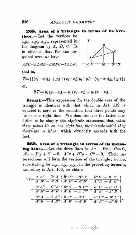
240 ANALYTIC GEOMETRY.
20$. Area of a Triangle in (onus of its Ver
tices. —Let the vertices be
x\H\i xsVv> represented in
the diagram by A, B, C. It
is obvious that for the re
quired area we have
ABC=ALMB+BMNC—CALN;
that is,
T=\{ (x—x,)(yi+y2)+(z3—x-^i+y^—{x —*i)(y3+yi) } ;
o4r rr
or,
2 T= yx (x2—x3) + ?/2 (a,—*,) + & a?).
Remark.—This expression for the double area of the
triangle is identical with that which in Art. 112 is
equated to zero as the condition that three points may
lie on one right line. We thus discover the latter con
dition to be simply the algebraic statement, that, when
three points lie on one right line, the triangle which they
determine vanishes: which obviously accords with the
fact.
2C9. Area of a Triangle in terms of its inclos
ing Liincs.—Let the three lines be Ax + By + C= 0,
A'x + B'y + C = 0, A"x + B"y + C" = 0. Their in
tersections will form the vertices of the triangle ; hence,
substituting for x${, x.,y2, xzyz, in the preceding formula,
according to Art. 106, we obtain
27'=O A' C A
A B' A' B
{ B' C"
I A' B"
— B"C B"C B C
C A" — C"A' [B"C
+ A' B" — A"B' \ ~F7B~
- A"B'
-B C"
+
C"A
~AFB
— G A"\B c
— A B"\A B'
■A B"
-B' O
A"B —A B"
B C —B'O
'A B' —A'B
B' C"—B
-A' B A' B" — A"B'
91\
B' Y
AREA OF A TRIANGLE. 247
Now if we reduce each of the sets of fractions inside the
braces to a common denominator, the three new numera
tors will be respectively
B" I B( C"A'—C A ") +B'{ CA"—C" A)+B//( C A—CA') \ ,
B \ B( C v A'—C A") +B'( GA"-C" A) +B"(C A-CA')\,
B' { B( G" A'-C A") +B'( GA"-C"A)+B"(CA- CA.') \ .
Hence, the final expression for the required area may be
written
{ B( G"A'—G'A") + B'( CA"—C"A)+B"(C'A—CA')*p
{AB'~A'B) {A'B^^A^B') {AB"—A"B)
Remark.—The numerator of this expression may be
otherwise written
\A"{BG'-B'G) + B'/{GA'—C/A) + G"{AB'-A'B)Y;
so that (Art. 113), if the three lines pass through the
same point, 2T vanishes. On the other hand, the
expression for 2T becomes infinite (Art. 96, Cor. 2)
whenever any two of the lines are parallel. In both
respects, then, the formula accords with the facts.
270. Ratio in which the Distance between
Two Points is divided by a Given Line.—Let
m : n be the ratio sought, and xxyx, x2y2 the given points.
The co-ordinates of division (Art. 52) will then be
mx2 + nxx my2 + nyxX m + w ' m -f- n
But these must of course satisfy the equation to the given
line ; hence,
A (mx2 -\- nXf) + B (?ny2 + nyt) + C (m + n) = 0.
m Axt + By^ + 0
n~~ Ax2 + By2 + 0 '
An. Ge. 24.

248 ANALYTIC GEOMETRY.
Corollary If the given line passed through two fixed
points x3y3 and xtyt, we should have (Art. 95, Cor. 1)
m_ (ffa — — fe — aQyt + a;^— y3st ' ■
» (2/3— y*)Xt — (a«— *4) i/2 + ztfi— ysx, '
as the raft'o m tvhich the distance between two fixed points
is divided by the line joining two others.
TRANSVERSALS.
271. Definition.—A Transversal of any system of
lines is a line which crosses all
the members of the system.
Thus, LMN is a transversal
of the three sides AB, BO, CA
in the triangle ABC.
272. Theorem.—In any triangle, the compound ratio
of the segments cut off upon the three sides by any trans
versal is equal to — 1.
In the above diagram, let the vertices A, B, 0 be
represented by a;,y„ x.2y2, x3y3, and the transversal LN
by Ax + By + C= 0. Then (Art. 270)
AL LB = - (Ax,+Byi+C) : (Ax.+Bt/.+ C),
BM:MC= — (Axt+Byt+C) : (Ax3+By3+C),
CN :NA =- (Ax.+By.+ C) : (Axx+Byi+C).
Multiplying these equations member by member, we
obtain the proposition.
273. Theorem.—In any triangle, the compound ratio
of the segments cut off upon the three sides by any three
convergents that pass through the vertices is equal to -\- 1.
For, if the point of convergency be 0, represented
by xty4 while the vertices are denoted as in the preceding

THREE CONVERGENTS. 249
article, we shall have (Art. 270, Cor.), after merely re
arranging the terms,
AP X\(y*--y3)+xi(y3--yi)+x3(y,--?/«)
PB~ -y«)+*«(yi-
BQ _x-i(yt--yi)+x,(y,---?/4) + .T4(j/1--*)
QC -y»)+*«(jfc- -2/4)
CR _My«- -.Vs)+a:4(.Va--?/»)
RA -yi)+xi(j/i--y«.)+*»(yi--2/2)
and the product of these equations is the algebraic
expression of the theorem.
We shall next give some illustrations of the uses of
abridged notation, as applied to rectilinear figures and
to right lines in general.
TRIPLE CONVERGENTS IN A TRIANGLE.
274. Theorem.—The three bisectors of the internal
angles of a triangle meet in one point.
For their equations are a—/9=0, /?—y—0, y—a=0 ;
and (Art. 114) these vanish identically when added
together.
275. Theorem.—The bisectors of any two external
angles of a triangle, and the bisector of the remaining
internal angle, meet in one point.
For their equations are a+/9=0, /9+^=0, y—a=0,
etc. But (Art. 108) y—a is a line passing through the
intersection of a+/9 and fi-\-y.
276. Theorem.—The three lines which join the vertices
of a triangle to the middle points of the opposite sides meet
in one point.
For (Ex. 2, p. 221) their equations are respectively
asinA—/3sin.B=0, /?sini5—^sinC=0, y sin G—a. sinA—0,
and therefore vanish identically when added together.

250 ANALYTIC GEOMETRY.
277. Theorem.—The three perpendiculars let fall from
the vertices of a triangle upon the opposite sides meet in
one point.
For (Ex. 3, p. 221) the corresponding equations are
acosA—/9cosjB=0,/9cosi?—^cosC=0,^cos(7—acosJ.=0.
278. Theorem.—The three perpendiculars erected at the
middle points of the sides of a triangle meet in one point.
For (Ex. 4, p. 221) we have found their equations
to be
a sin A — /3 sin B + 7 ain {A—B) = 0,
PsinS — ysin C+ a sin (J5— C) =0,
ysin C — a sin .4 + /3sin (C—A) = 0;
and, if we multiply these by sin2C, sin2A, sin2!? respect
ively, we shall cause them to vanish identically. (See
Trig., 850, Ex. 2.)
HOMOLOGOUS TRIANGLES.
279. Definitions.—Two triangles, the intersections of
whose sides taken two and two lie on one right line, are
said to be homologous.
The line on which the
three intersections lie is
called the axis of homology.
Any two sides that form
one of the three intersec
tions are termed corre
sponding sides ; and the
angles opposite to them,
corresponding angles.
Thus, in the diagram, the triangles ABC, A'B'C are
homologous with respect to the axis LMN. AB, A'B';
BC, B'C ; CA, C'A' are the corresponding sides; and
A, A'; B, B'; C, C, the corresponding angles.

HOMOLOO Y. 251
2S0. Theorem.—In any two homologous triangles, the
right lines joining the corresponding vertices meet in one
point.
Let a, /?, y be the sides of ABO, and take the latter
for the triangle of reference ; the equation to the axis
LN may then be written la + m/9 + ny = 0. Suppose
the Cartesian origin to be somewhere between the tri
angles, and (Art. 108, Cor. 2) the equations to A'B',
B'C, C'A', which pass through the intersections of
a, jS, y with the axis, will be
{l—l')a+mp+ny=-<i, la+(m—m/)[}+ny=0, fo+m/3+(n—7i')y=0.
Subtracting the second of these from the first, the third
from the second, and the first from the third, we get
I'a — m'P= 0, tm'/9 — n'y = 0, n'y — I'a = 0.
But these equations (Art. 107) evidently denote the lines
BB', CO', AA'; and they vanish identically, when added
together.
Remark.—The point in which the lines joining the
corresponding vertices meet, is called the center of
homology.
281. Theorem.—If the lines joining the corresponding
vertices of two triangles meet in one point, the intersections
of the corresponding sides lie on one right line.
This theorem, the converse of the preceding, is ob
tained at once by merely interpreting the equations of
the foregoing article in tangentials. We leave the student
to carry out the details.
COMPLETE QUADRILATERALS.
282. Definitions.—A Complete Quadrilateral is
the figure formed by any four right lines intersecting in
six points.

252 ANALYTIC GEOMETRY.
The three remaining right lines by c
which the six points of intersection f\
can be joined two and two, are called / \\ /
the diagonals of the quadrilateral. F/ \ W
Thus, ABCDEF is the complete \
quadrilateral of the four lines AB, / ^2-^^"-\
BE, EF, FA, which meet in the six a bT>
points B, E,F,A, C, D. AE, BF are
the two inner diagonals, and CD is the outer one, some
times called the third.
283. Theorem.—In any complete quadrilateral, the
middle points of the three diagonals lie on one right line.
Let a, /9, y, 8 be the equations to the four sides of the
quadrilateral, and let the respective lengths of BE, EF1,
FA, AB equal a, b, c, d. Then L, M, N being the middle
points of the three diagonals, we have the following equa
tions to the lines drawn from the vertices to the middle
points of the bases of the triangles ABE, EFA, ABF,
FEB:
dd — aa = 0 (BL), b@ — cr = 0 (FL) ;
cr —dS.= 0 (AM), aa — 6/9 = 0 (EM).
Hence, L and M both lie upon the line
aa— bp + c-r — dd = 0 (1),
as this obviously passes through the intersection of
(BL, FL), and of (AM, EM). If we now put Q = the
double area of ABEF, we shall have
aa + bj3 + cr + dd= Q,
and thence
aa — bp + cy — dd = 2 (aa + cy) — Q,
aa — bp + cr—dS =—2 (6/9 + dd) + Q.
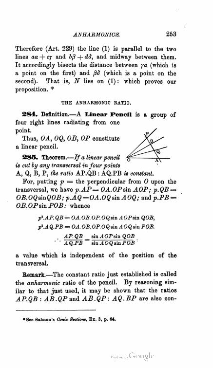
ANHARMONICS. 253
Therefore (Art. 229) the line (1) is parallel to the two
lines aa -f- cy and 6/9 -f dd, and midway between them.
It accordingly bisects the distance between ya (which is
a point on the first) and [33 (which is a point on the
second). That is, N lies on (1) : which proves our
proposition. *
THE ANHARMONIC RATIO.
284. Definition.—A Linear Pencil is a group of
four right lines radiating from one
point.
Thus, OA, OQ, OB, OP constitute
a linear pencil.
2S5. Theorem.—If a linear pencil
is cut by any transversal in four points
A, Q, B, P, the ratio AP.QB : AQ.PB is constant.
For, putting p — the perpendicular from 0 upon the
transversal, we have p.AP= OA.OP&m AOP ; p.QB=
OB.OQsinQOB; p.AQ =OA.OQ sin AOQ; and p.PB=
OB.OP sin POB: whence
p\APQB = OA.OB.OP.OQsin AOPsin QOB,
piA Q.PB = OA. OB. OP.OQ sin AOQ sin POB.
AP.QB _ sin A OP sin QOB"'■ AQ.PB~ sin AOQ sin POB
a value which is independent of the position of the
transversal.
Remark.—The constant ratio just established is called
the anharmonic ratio of the pencil. By reasoning sim
ilar to that just used, it may be shown that the ratios
AP.QB : AB.QPand AB.QP : AQ.BP are also con-
*See Salmon's Conic Sections, Ex. 3, p. 64.
254 ANALYTIC GEOMETRY.
stant. To these, accordingly, the term anharmonic is at
times applied ; but it is generally reserved for the par
ticular ratio to which we have assigned it, and we shall
always intend that ratio when we use it hereafter.
Note—The Anharmonic Ratio has an important place in the
Modern Geometry, especially in connection with the doctrine of the
Conic. Its existence, however, has been known since the time of
the Alexandrian geometer Pappus, who gives the property in his
Mathematics Collecliones, Book VII, 129, and who probably belongs
to the fourth century. The name anharmonic was given by Chasles.
But the bearing of the ratio upon the new geometry had been pre
viously investigated by Mobius, who called it the Ratio of Double
Section (Doppelschnittsverhaltniss).
286. Definition.—An Harmonic Proportion sub
sists between three quantities, when the first is to the
third as the difference between the first and second is to
the difference between the second and third.
Thus, if the pencil in the .above diagram cut the trans
versal so as to make AP-.AQ :: AP—AB : AB — AQ,
the whole line AP would be in harmonic proportion with
its segments AB and AQ.
Corollary.—A line is divided harmonically, when it is
cut into three segments such that the whole is to either
extreme as the other extreme is to the mean. For the
proportion given above may obviously be written
AP : AQ :: BP: BQ.
287. Definitions.—An Harmonic Pencil is one
which cuts its transversals harmonically.
I. From the final equation of Art. 285, it is evident
that when the anharmonic ratio of a pencil is numerically
equal to 1, the pencil is harmonic.
II. The four points in which a line is cut by an har
monic pencil, are called harmonic points.

HARMONIC PENCILS. 255
III. Linear pencils are in general termed anharmonic,
because they do not in general cut off harmonic segments
from their transversals.
288. Theorem.— The anharmonic of the pencil formed
by the four lines a, ft, a + kft, a + k'ft is equal to k : k'.
Let OA be the position of a,
OB of ft, OP of a + kft, and OQ of
a + Then, A; being the ratio of
the perpendiculars from OP upon
O.A, OP, and k' the ratio of those
from OQ on the same lines, we shall
have &=sin AOP: sin POP, and F=sin ^100. : sin QOB.
Hence, ^ ^ sin ^ OP sin QOP .
. k>~ sin AOQ sin POB'
which (Art. 285) proves the proposition.
Corollary.—If k' = — k, the anharmonic of the pencil
becomes numerically equal to 1. Hence (Art. 287, I)
the important property : The four lines a, ft, a + kft,
a — kft form an harmonic pencil.
Also, by the analogy of tangentials : The four points
a, ft, a-\- kft, a — left are harmonic.
2S9. Theorem.—The anharmonic of any four lines
a + kft, a-^-lft, a + mft, a-\-nft is equal to
(n — k) (m — Z)
(n — m) (I — k)
Let OA, OB represent the lines
a and ft, and OK, OL, OM, ON the
four lines a-{-kft, a-\-lft, a-\-mft, a-\-nft.
Then, if rs be any transversal, the
anharmonic of the four given lines
will be au.eo : ae.ou; or, what
amounts to the same thing, it will be
An. Ge. 25.

256 ANALYTIC GEOMETRY.
(ru—ra) (ro — re) : (re— ra) (ru — ro). Now, taking the
lengths of the perpendiculars from a, e, o, u upon a, both
trigonometrically and from the equations to the given
lines, we obtain
ru =— rift cosec Ors, ra=— kft cosec Ors,
ro = —mft cosec Ors, re =— Ift cosec Ors.
Substituting these values in the ratio last written, and
recollecting that, since the anharmonic is independent
of the position of the transversal, we may take rs parallel
to the line ft, and thus render the perpendicular ft a
constant, we find after reductions
B== (n — jO (m — 0 .
(n — m) (I — k)
Remark.—The student can easily convince himself
that the harmonic and anharmonic properties above
obtained are true for lines whose equations are of the
more general form L = 0, M= 0, L -f- kM= 0, etc.
290. Theorem.—If there be two systems of right lines,
each radiating from a fixed point, and if the several mem
bers of the one be similarly situated with those of the other
in regard to any two lines of the respective groups, then
will the anharmonic of any pencil in the first system be
equal to that of the pencil formed by the four correspond
ing lines of the second.
For, in such a case, the two reference-lines of the
first group being L = 0, U= 0, and those of the second
M=0, M'=0, the corresponding pencils will be (L-\-kLr,
L + W, L + ml/, L + nL') and (M+ kM', M+ IM',
M+mM', M+nM'). Hence, the theorem follows
directly from the result of Art. 289.

NOMOGRAPHIC LINES. 257
291. Definition.—Systems of lines whose correspond
ing pencils have equal anharmonics are called homographic
systems.
Thus, in the diagram of Art. 289, the two systems
{OA, OK, OL, OM, ON, OB) and {O'A, O'K', O'L',
O'M', O'N', O'B) are intended to represent a particular
case of homographics.
292. In the examples which follow, some are best
adapted for solution by the old notation, and others by
the abridged. We have room for only a few of the
manifold properties of the Right Line.
EXAMPLES.
1. If from the vertices of any triangle any three convergents be
drawn, and the points in which these meet the opposite sides be
joined two and two by three right lines, the points in which the
latter cut the sides again will lie on one right line.
2. Any side of a triangle is divided harmonically by one of the
three convergents mentioned in Ex. 1, and the line joining the feet
of the other two.
3. In the figure drawn for the two preceding examples, deter
mine by tangentials all the points that are harmonic.
4. In any triangle, the two sides, the line drawn from the vertex
to the middle of the base, and the parallel to the base through the
vertex, form an harmonic pencil.
5. The intersection of the three perpendiculars to the sides of a
triangle, the intersection of the three lines drawn from the vertices
to the middle points of the sides, and the center of the circum
scribed circle, lie on one right line.
6. APB, CQD are two parallels, and AP-.PB:: DQ: QC: to
prove that the three right lines AD, PQ, BC are convergent.
7. From three points A, B, D, in a right line ABCD, three con
vergents are drawn to a point P; and through C is drawn a right
line parallel to AP, meeting PB in E and PD in F: to prove that
AD.BC: AB.CD:: EC: CF.
258 ANALYTIC GEOMETRY.
8. The six bisectors of the angles of any triangle intersect in
only four points besides the vertices.
9. If through the vertices of any triangle lines be drawn parallel
to the opposite sides, the right lines which join their intersections
to the three given vertices will meet in one point. [Use both notations
in succession.]
10. If through the vertices of any triangle there be drawn any
three convergents whatever, to prove that these three lines and the
three sides of the triangle may be respectively represented by the
equations
v — w = 0, w — u = 0, u — t> = 0,
w + to = A, to + u = /l, u + v = ^.
11. ItOAA'A", OBB'B" are two right lines harmonically
divided, the former in A and A', the latter in B and B', the lines
AB, A'B', A"B" either meet in one point or are parallel.
12. If on the three sides of a triangle, taken in turn as diagonals,
there be constructed parallelograms whose sides are parallel to two
fixed right lines, the three remaining diagonals of the parallelograms
will meet in one point.
13. The three external bisectors of the angles of any triangle
meet the opposite sides in three points which lie on one right line.
14. If three right lines drawn from the vertices of any triangle
meet in one point, their respective parallels drawn through the
middle of the opposite sides also meet in one point.
15. In every quadrilateral, the three lines which join the middle
points of the opposite sides and the middle points of the diagonals,
meet in one point.
16. If the four inner angles A,B,E,F of a complete quadrilateral
(see diagram, Art. 219) are bisected by four right lines, the diago
nals of the quadrilateral formed by these bisectors will pass through
the two outer vertices of the complete one, namely, one through C
and the other through D.
17. Let the two inner diagonals of any complete quadrilateral
(same diagram) intersect in O : the diagonals of the two quadri
laterals into which either CO or DO divides ABEF, intersect in
two points which lie on one right line with O.
18. In any complete quadrilateral, any two opposite sides form
an harmonic pencil with the outer diagonal and the line joining
their intersection to that of the two inner diagonals.

PROPERTIES OF THE CIRCLE. 259
19. Also, the two inner diagonals are harmonically conjugate to
the two lines which join their intersection to the two outer vertices.
20. Also, two adjacent sides are harmonically conjugate to their
inner diagonal and the line joining their intersection to that of the
outer diagonal and the remaining inner one; etc.
CHAPTER SECOND.
THE CIRCLE.
293. Before attempting the discussion of the three
Conies strictly so called, it will be advantageous to
illustrate the analytic method by applying it to that
case of the Ellipse with whose properties the reader
is already familiar from his studies in pure geometry :
we mean, of course, the Circle. As we proceed in this
application, we shall be enabled to define those elements
of curves in general, which constitute at once the leading
objects and principal aids of geometric analysis.
THE AXIS OF X.
294. The rectangular equation to the Circle referred
to its center (Art. 136) is
x2 -j- y2 = r2.
If we solve this for y, we obtain
y —V{r+x) (r—x). But, from x'-
the diagram, r + x = AM, and
r — x = MB ; and we have the
well-known property of Geom.,
325,
The ordinate to any diameter of a circle is a mean
proportional between the corresponding segments.

260 ANALYTIC GEOMETRY.
295. If we eliminate between the equation to a circle
x2 -(- y2 = r2 and that of any right line y = mx + b by
substituting for y in the former from the latter, we
shall obtain, as determining the abscissas of intersection
between a right line and a circle, the quadratic
(1 + m2) x2 + 2mb.x + b2 — r2 = 0.
Now the roots of this quadratic are real and unequal,
equal, or imaginary, according as (1 + m2) r2 is greater
than, equal to, or less than b2. Hence, when the first of
these conditions occurs, the right line will meet the circle
in two real and different points ; when the second, in two
coincident points ; when the third, in two imaginary points.
Adhering, then, to the distinction between these three
classes of points, we may assert, with full generality,
Every right line meets a circle in two points, real, coin
cident, or imaginary.
296. It is so important that the distinction just
alluded to shall be exactly understood in our future
investigations, that we consider it worth while to
illustrate it somewhat more at length.
I. The conception of two real points, situated at a
finite distance from each other, is of course already clear
to the student. We therefore merely add, that such points
are sometimes called discrete, or discontinuous points.
II. The conception of coincident, or, as they are more
significantly called, consecutive points, is peculiar to the
analytic method. The most general definition of con
secutive points is, that they are points whose distance from
each other is infinitely small. It may aid in rendering this
definition clear, to think of two points which are drawing
closer and closer together, which tend to meet but not

CONSECUTIVE POINTS. 261
to pass each other, and whose mutual approach is never
for an instant interrupted. The distance between two
such points is evidently less than any assignable quantity ;
for however small a distance we may assign as the true
one, the points will have drawn nearer together in the
very instant in which we assign it : so that their distance
eludes all attempts at finite statement, and can only be
represented by the phrase infinitely small.
The geometric meaning of this analytic conception
varies with its different applications. Thus, it may sig
nify exactly the same thing as the single point which, in
the language of pure geometry, is common to a curve
and its tangent. For since the distance between con
secutive points is infinitely small ; that is, so small that
we can not assign a value too small for it ; we may
assign the value 0, and take the points as absolutely
coincident. It is in this aspect, mainly, that we shall
use the conception in our future inquiries. Hence, as
from the infinite series of continuous values which the
distance between two consecutive points must have, we
thus select the one corresponding to the moment of
coincidence, we have preferred to designate the concep
tion by the equivalent and for us more pertinent phrase
coincident points.
The student should be sure that he always thinks of
the distance between coincident points as a true infinit
esimal. The error into which the beginner almost always
falls is, to think of a very small, instead of an infinitely
small, distance. He thus confounds with two consecutive
points, two discrete ones extremely close together, between
which there is of course a finite distance. The conse
quence is, that he finds in such a distance, however small,
an infinite number of points lying between his supposed
consecutives, and fancies that all the arguments based
262 ANALYTIC GEOMETRY.
on the conception of consecutiveness are fallacious.
Whereas, if he excludes from his thoughts, as he should,
all points separated by any finite distance however small,
he will have points absolutely consecutive, in the only
sense that mature reflection attaches to that term.
III. The phrase imaginary points is also peculiar to
analytic investigation. It really means, when translated
into the language of pure geometry, that the correspond
ing points not only do not exist, but are impossible. But, as
we have mentioned once before, the expression, together
with the accessories which serve to carry out its use, is
found to be of real value in developing certain remote
analogies in the properties of curves. We shall therefore
retain it, only cautioning the student not to be misled
by a false interpretation of it.
297. Definition.—A Cbord of any curve is any right
line that meets it in two points.
298. Equation to a Circular Chord.—Let the
equation to the given circle be x2 + y2 = r2. Since
the chord passes through two points of the curve, its
equation (Art. 95) will be of the form
in which xfy', x"y", since they both lie upon the circle,
y — y' _ y"—y' .
x — x' x"—x>'
are subject to the condition
Hence, a/2 — xm — y'n— y'2; and we obtain
y"-y' _
x"—x'~
x' + x'
y'+y

CHORD AND DIAMETER. 263
Therefore the required equation to a chord is
y — y' x' x" .
x — x' y' -\- y"
in which x'y', x"y" are the points in which the chord
cuts the circle.
Corollary.—By a course of analysis exactly similar to
that just used, we find the equation to any chord of the
circle (x — g)2 -(- (y —/)2 = r2, namely,
y — y'_ x' + x" — 2g
x — x'~~y' + y" — 2f
in which x'y', x"y" are the intersections of the circle
with its chord, and gf is its center.
DIAMETERS.
299. Definition.—A Diameter of any curve is the
locus of the middle points of parallel chords.
300. Equation to a Circular Diameter.—To
find this, we must form the equation to the locus of
the middle points of parallel chords in a circle. Let
x, y be the co-ordinates of any middle point : the
formula for the length of the chord from xy to the
point x'y' of the curve (Art. 102) gives us either
x' =x-j- cl or y' = y + si.
But since x'y' is a point on the circle x2 + y2 — r2, we
have
(x + ct)2 + (y + siy = r2;
or, remembering that s2+ c2 = 1, we get, for determining
the distance I of the point xy from the circle, the quadratic
l2 + 2(cx+sy)l+ (x2 + y2— r2) = 0.
264 ANALYTIC GEOMETRY.
Now, as xy is the middle point of a chord, the two values
of I in this quadratic must be numerically equal with
contrary signs. Hence, (Alg., 234, Prop. 3d,) the co
efficient of I must vanish, and we get
ex-\- sy = 0.
But, in the present inquiry, s and c are the sine and
cosine of the angle which a chord through xy makes
with the axis of x; and as this angle is the same for
all parallel chords, the equation
cx + sy = 0
is a constant relation between the co-ordinates of the
middle points of a series of parallel chords. That is,
it is the required equation to any diameter of the
circle.
301. If 6 be the inclination of a series of parallel
chords to the axis of x, the equation just obtained may
be written y=— xcotd. Hence, (Arts. 63; 96, Cor. 3,)
we have the familiar property,
Every diameter of a circle passes through the center,
and is perpendicular to the chords which it bisects.
Corollary.—From this we immediately obtain the im
portant principle : If a diameter bisects chords parallel to
a second, the second bisects those parallel to the first.
302. Definition.—By Conjugate Diameters of a
curve, we mean two diameters so related that each bisects
chords parallel to the other.
303. We have seen (Art. 301) that the equation to
any diameter of a circle may be written y — — x cot 0,
in which expression d is the inclination of the chords
<
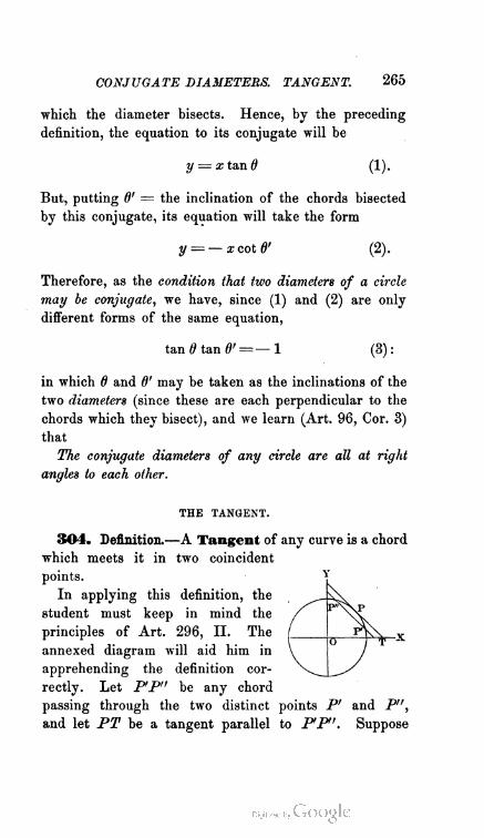
CONJUGATE DIAMETERS. TANGENT. 265
which the diameter bisects. Hence, by the preceding
definition, the equation to its conjugate will be
y — xtund (1).
But, putting 0' = the inclination of the chords bisected
by this conjugate, its equation will take the form
y = — xcotd' (2).
Therefore, as the condition that two diameters of a circle
may be conjugate, we have, since (1) and (2) are only
diiferent forms of the same equation,
tan 0 tan 0' =—l (3):
in which 0 and 6' may be taken as the inclinations of the
two diameters (since these are each perpendicular to the
chords which they bisect), and we learn (Art. 96, Cor. 3)
that
The conjugate diameters of any circle are all at right
angles to each other.
THE TANGENT.
304. Definition.—A Tangent of any curve is a chord
which meets it in two coincident
points.
In applying this definition, the
student must keep in mind the
principles of Art. 296, II. The
annexed diagram will aid him in
apprehending the definition cor
rectly. Let P'P" be any chord
passing through the two distinct points P' and P",
and let PT be a tangent parallel to P'P". Suppose
266 ANALYTIC GEOMETRY.
PP' to move parallel to itself until it coincides with
PT. It is evident that as PP' advances toward PT,
the points P' and P" will move along the curve toward
each other, and that when P'P' at length coincides with
PT, they will become coincident in P, which is called the
point of contact. We shall often allude to the position
of the two coincident points through which a tangent
passes, by the term contact alone.
305. Equation to a Tangent of a Circle.—Let
the given circle be represented by x2 -f y2 — r2. Then,
to obtain the required equation, we have only to suppose,
in the equation to any chord (Art. 298), that the co-ordi
nates x' and x", y' and y", become identical. Making this
supposition, reducing, and recollecting that x'2 -f- y'2 = r2,
we obtain
x'x + y'y = r2 :
in which x'y' is the point of contact.
Corollary.—To obtain the equation to a tangent of
the circle (x — <7)2+(«T—fY — r2, which diners from
x2 -\- y2= r2 only in having the origin removed to the
point (— g, —/), we simply transform the expression
just found to parallel axes passing through the last-
named point, by replacing x and y, a;' and y', by x — g,
y—/, x'— g, y'—/. We thus get
■. V-g)(x-g) + (y'-f) {y-f)=r>.
We may also obtain this less directly, by applying the
condition for coincidence to the equation in the corollary
to Art. 298.
306. Condition that a right line shall touch a
Circle.—In order that the line y = mx + b may touch
the circle x2 + y2 = r2, it must intersect the latter in two

EQUATION TO TANGENT. 267
coincident points ; that is, the co-ordinates of its two in
tersections with the circle must become identical. Hence,
the required condition will be found by eliminating between
y — mx + b and x2 -\- y2 — r2, and forming the condition
that the resulting equation may have equal roots.
The resultant of this elimination is the quadratic
(1 + wi2) x2 + 2mb.x + (b2 — r2) = 0 ;
and (see third equation of Art. 127, et seq.) the condition
that this may have equal roots is
m2b2=(l + m2) (b1 — r2) .-. 6= rl/l + m2.
Corollary.—Hence, every line whose equation is of the
form
y = mx + r V\ + m2,
touches the circle x2 + y2= r2. This equation belongs to
a group of analogous expressions for the tangents of the
several Conies; and, on account of its great usefulness,
especially in problems where the point of contact is not
involved, is called the Magical Equation to the Tangent.
307« Anxlliary Angle In problems that concern the in
tersection of lines with a circle, it is often advantageous to express
the co-ordinates of the point on the curve in terms of the angle which
the radius drawn to such point makes with the axis of x. By so doing,
we obtain formulae involving only one variable.
Thus, if V= the angle POM, it is evi
dent that we shall have, for the co-ordi
nates of any point JF",
x/ = rcosS/, y'=r&m8'.
In this notation, the equation to any
chord P'P" becomes (see Art. 298)
x cos i + y sin } (6"+ef) = r cos \ :
268 ANALYTIC GEOMETRY.
in which V = the angle POM, and 0" = the angle P"OM'.
Hence, the corresponding equation to any tangent is
x cos V + y sin W = r.
This may also be obtained by substituting directly in the equation
ofArt 305; and it expresses (Art. 80, Cor.) the well-known property,
that the tangent to a circle is perpendicular to the radius at contact
308. To draw a Tangent to a Circle from a
Fixed Point.—This problem, so far as it belongs to
analytic investigation, requires us to find the point of
contact corresponding to the tangent which passes'
through the arbitrary point x'y' .
Let x"y" be the unknown point of contact. The
equation to the tangent is then (Art. 305)
x"x + y"y — r2.
But, since this tangent is drawn through x'y', we have
x"x' + y"y' = r2 (1).
Moreover, since x"y" is upon the circle,
a.^2 + y/2 = r2 (2).
Solving for x" and y" between (1) and (2), we get the
co-ordinates of the point of contact, namely,
„ r2x'±ry'V/xl2+y'2—r2 _ r'y'^rx'Vx'^y'2—r2
" x'*+y'2 ' & ~~ x'2 + y'2
Corollary.—Hence, through any fixed point there can
be drawn two tangents to a given circle, real, coincident,
or imaginary. Meal, when x'2 + y'2 > r2 ; that is, when
x'y' is outside the circle. Imaginary, when x'2 + !//2<r2;
that is, when x'y' is within the circle. Coincident, when
z?2 + yn — 72 j that is, when x'y' is on the circle.
LENGTH OF TANGENT. 269
309. Length of the Tangent from any point
to a Circle.—Let xy be any point in the plane of a
circle whose center is the point gf. Then (Art. 51,
I, Cor. 1) for the square of the distance between xy
and gf, we have
S2 = (x-g)2+(y-f)2.
Putting t = the required length of the tangent, we get
(since the tangent is perpendicular to the radius at
contact) t2 = 82 — r2. That is,
t2={x-g)2+(y-f)2-r2.
From this we learn that if the co-ordinates x and y of
any point be substituted in the equation to any circle, the
result will be the square of the length of the tangent drawn
from that point to the circle.
Remark.—We have shown (Art. 142) that the general
equation
A (x2 + y2) + 2Qx + 2Fy + 0= 0
is equivalent to (x — g)2 + (y —f)2 = r2, provided we
take out A as a common factor. Hence, the property
just proved applies to every equation denoting a circle,
provided it be reduced to the form in question by the
proper division. If, then, we write S as a convenient
abbreviation for the left member of the equation to a
circle, in which the common co-efficient of x2 and y2 is
unity, we get
Corollary—The square of the length of the tangent
from the origin of the circle.
A {3? + y2) + 2Gx + 2Fy+C= 0,
is equal to C: A; that is, to the quotient of the absolute
term by the common co-efficient of x2 and y2.
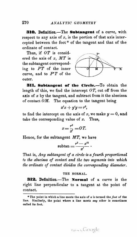
270 ANALYTIC GEOMETRY
310. Definition.—The Subtangent of a curve, with
respect to any axis of x, is the portion of that axis inter
cepted between the foot * of the tangent and that of the
ordinate of contact.
Thus, if 027 is consid- P,
ered the axis of x, MT is
the subtangent correspond-
\° M 1 T Xing to PT of the inner
curve, and to PT of the
outer.
311. Subtangent of the Circle.—To obtain the
length of this, we find the intercept OT, cut off from the
axis of x by the tangent, and subtract from it the abscissa
of contact OM. The equation to the tangent being
x'x + y'y = r2,
to find the intercept on the axis of x, we make y — 0, and
take the corresponding value of x. Thus,
r2
x=-, =0T.
x?
Hence, for the subtangent MT, we have
r2 — xn
subtan = ;—■ •
x'
That is, Any subtangent of a circle is a fourth proportional
to the abscissa of contact and the two segments into which
the ordinate of contact divides the corresponding diameter.
THE NORMAL.
313. Definition.—The Normal of a curve is the
right line perpendicular to a tangent at the point of
contact.
* The point in which a line meets the axis of x is termed the foot of the
line. Similarly, the point where a line meets any other is sometimes
called its foot.

NORMAL AND SUBNORMAL. 271
313. Equation to a Normal of a Circle.—Since
the normal is perpendicular to the line x'x-\-y'y= r2, and
passes through the point of contact x'y', its equation (Art.
103, Cor. 1) is
V — */'=f> ix — x');
or, after reduction,
y'x — x'y = 0.
The form of this expression (Art. 95, Cor. 2) shows
that every normal of a circle passes through the center : —
a property which we might have gathered at once from
the definition.
314. Definition.—The portion of the normal included
between the point of contact and the axis on which the cor
responding subtangent is measured, is called the length of
the normal. For example, P'O in the diagram of Art. 310.
From the result of Art. 313, it follows that the length of
the normal in any circle is constant, and equal to the radius.
315. Definition.—The Subnormal of a curve, with
respect to any axis of x, is the portion of that axis inter
cepted between the foot of the normal and that of the
corresponding ordinate of contact.
Thus, in the diagram of Art. 310, OM is the subnormal
corresponding to the point P1.
Hence, for the Circle, we have
subnor = x'.
That is, Any subnormal of a circle is equal to the corre
sponding abscissa of contact.
SUPPLEMENTAL CHOEDS.
316. Definition.—By Supplemental Chords of a
circle, we mean two chords passing respectively through
the extremities of a diameter, and intersecting on the curve.
An. Ge. 26.
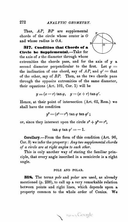
272 ANALYTIC GEOMETRY.
Thus, AP, BP are supplemental
chords of the circle whose center is 0
and whose radius is OA.B
317. Condition that Chords of a
Circle be Supplemental.—Take for
the axis of x the diameter through whose
extremities the chords pass, and for the axis of y a
second diameter perpendicular to the first. Let f ==
the inclination of one chord, say of AP, and f' = that
of the other, say of BP. Then, as the two chords pass
through the opposite extremities of the same diameter,
their equations (Art. 101, Cor. 1) will be
y = (x— r) tan f, y—(x-\- r) tan <p'.
Hence, at their point of intersection (Art. 62, Rem.) we
shall have the condition
y2 = (x2— r2) tan <p tan <p' ;
or, since they intersect upon the circle x2 -\- y^—r2,
tan f tan f' = — 1.
Corollary.—From the form of this condition (Art. 96,
Cor. 3) we infer the property : Any two supplemental chords
of a circle are at right angles to each other.
This is only another way of stating the familiar prin
ciple, that every angle inscribed in a semicircle is a right
angle.
POLE AND POLAR.
318. The terms pole and polar are used, as already
mentioned (p. 238), to call up a very remarkable relation
between points and right lines, which depends upon a
property common to the whole order of Conies. We
\

POLE AND POLAR. 273
shall now endeavor to develop the conception of the
pole and polar with respect to the Circle, in the order
according to which they naturally appear in analysis.
319. Chord of Contact belonging to Two Tan
gents which pass through a Fixed Point.—By
the chord of contact here mentioned, we mean the right
line joining the two points of contact corresponding to
the pair of tangents which (Art. 308, Cor.) we have seen
can be drawn to a circle from any external point. Let
x'y' be the fixed external point, and xiy„ x2y2 the two
corresponding points of contact. The equations to the
two tangents (Art. 305) will then be
*is+yiy=r*, x2x + y2y=r2.
Now, since both the tangents pass through x'y', we have
the two conditions
*\x? +ytf= rt, x2x' + y2y' = r2.
Hence, the co-ordinates of both points of contact satisfy
the equation
x'x + y'y = r2 :
which is therefore the equation to the chord of contact.
320. Locus of the intersection of Tangents at
the extremities of a Chord passing through a
Fixed Point.—Let x'y' be the fixed point through
which the chord passes, and x<yx the point in which the
two tangents drawn at its extremities intersect. The
equation to the chord (Art. 319) will be x^x-\-y{y = r2;
and, as x'y' is a point on the chord, we shall have the
condition

274 ANALYTIC GEOMETRY.
no matter what be the direction of the chord. Hence,
supposing the chord to be movable, and the intersection
of the two corresponding tangents to be a variable point,
the co-ordinates of the latter will always satisfy the
equation
x'x + y'y — r2 :
which is therefore the equation to the locus required,
and shows (Art. 85) that this locus is a right line.
321. Relation of the Tangent to this Locus
ami to the Chord of Contact.—The equation to the
chord of contact of the two tangents drawn from any
point outside of a circle, is
x'x + y'y= r2 (1),
in which x'y' is the point from tohich the tangents are
drawn. The equation to the locus of the intersection
of two tangents drawn at the extremities of any chord
passing through a fixed point, is
x'x + y'y=r2 (2),
in which x'y' is the point through which the movable chord
is drawn. The equation to any tangent of the same circle
to which the chord (1) and the locus (2) refer, is
x'x + y'y = r2 (3),
in which x'y' is the point of contact. What, then, is the
significance of this remarkable identity in the equations
to these three lines? It certainly means that there is
some law of form common to the tangent, the chord of
contact, and the locus mentioned. For (1), (2), (3) assert
that the chord of contact is connected with the point
from which the two corresponding tangents are drawn,
and that the right line forming the locus of the inter

POLE AND POLAR. 275
section of two tangents at the extremities of a chord
passing through a fixed point is connected with that
point, in exactly the same way that the tangent is con
nected with its point of contact. Now a right line in
the plane of a circle must he either a tangent, a chord
of contact, or a locus corresponding to (2): hence we
learn that the Circle possesses the remarkable property
of imparting to any right line in its plane the power
of determining a point ; and reciprocally.
This property is known as the principle of polar re
ciprocity ; or, as it is sometimes called, the principle of
reciprocal polarity. It is fully expressed in the following
twofold theorem :
I. Iffrom a fixed point chords be drawn to any circle,
and tangents to the curve be formed at the extremities of
each chord, the intersections of the several pairs of tangents
will lie on one right line.
II. Iffrom different points lying on one right line pairs
of tangents be drawn to any circle, their several chords of
contact will meet in one point.
The truth of (I) is evident from the equation of Art. 320 ;
that of (II) appears as follows : — Let Ax-\-By+C=Q be
any right line. The chord of contact corresponding to
any point x'y' of this line (Art. 319) is x'x-\- y'y = rl.
Now the co-efficients of this equation are connected by
the linear relation
Ax' + By' + C=0,
and the chord passes through a fixed point by Art. 117.
We shall find, as we go on, that the property just
proved of the Circle is common to all conies. The
reciprocal relation between a point and a right line is
expressed by calling the point the pole of the line, and
the line the polar of the point.

276 ANALYTIC GEOMETRY.
Definitions.—The Polar of any point, with
respect to a circle, is the right line which forms the locus
of the intersection of the two tangents drawn at the ex
tremities of any chord passing through the point. Thus,
LL'L" is the polar of P.
The Pole of any right line, with respect to a circle,
is the point in which all the chords of contact corre
sponding to different points on the line intersect each
other. Thus, P is the pole of LL'L".
These definitions
enable us to con
struct the polar when
the point is given,
or the pole when we
have the line. Thus,
if P be the point, we
draw any two chords
through it, as MPN,
OPQ, and the corre
sponding pairs of tan
gents, ML,NL; OL",
QL". The line which
joins the points L and
L", in which the re
spective pairs of tangents intersect, is the polar of P.
On the other hand, if LL" be the given line, we draw
from any two of its points, as L and L", two pairs of
tangents, LM,LN; L"0,L"Q, and the two correspond
ing chords of contact, MN, OQ: the point P in which
the latter meet, is the required pole.
We have given the construction in the form above be
cause it answers in all cases. It is evident, howrever, from
the results of Art. 321, that when P is without the circle,
its polar is the corresponding chord of contact QR; and
CONSTRUCTION OF POLAR. 277
that when it is on the curve, its polar is the corresponding
tangent I'S. In these cases, then, our drawing may be
modified in accordance with these facts.
323. From all that has now been shown, it follows
that the equation to the polar of any point x'y', with
respect to the circle x2 + y1 — r2, is
x'x + y'y = r2.
Now the equation to the line which joins x'y' to the center
of the same circle (Art. 95, Cor. 2) is
y'x — x'y - 0.
Hence, (Art. 99,) The polar of any point is perpendicular
to the line which joins that point to the center of the corre
sponding circle.
Corollary.—This property affords a method of con
structing the polar, simpler than that explained in the
preceding article. For (Art. 92, Cor. 2) the distance
of the polar from the center of its circle is
r2
in which (Art. 51, I, Cor. 2) Vxn -f yn is the distance
of the pole from the center ; hence, To construct the polar,
join the pole to the center of the circle, and from the latter
as origin lay off upon the resulting line a distance forming
a third proportional to its whole length and the radius:
the perpendicular to the first line, drawn through the point
thus reached, will be the polar required.
In the next four articles, we will present a few striking
properties of polars.

278 ANALYTIC GEOMETRY.
324. The condition that a point x"y" shall lie upon the polar
of x'y' is of course
Now, obviously, this is also the condition that x'y' shall lie upon
the polar of x"y". Therefore, If a point lie upon the polar of a
second, the second will lie upon the polar of the first.
Corollary—Hence, The intersection of two right lines is the pole
of the line which joins their poles.
Bemark.—We shall find hereafter that these properties are com
mon to all conies.
325. The distance of x'y' from the polar of x"y" (Art 105,
Cor. 2) is
x"x'+i/y— r2
and the distance of x"y" from the polar of x'y' is
xfx"+yfy"-r'
W+y")
Hence, The distances of two points from each other s polars are pro
portional to their distances from the center of the corresponding circle.
326. Definitions—Two triangles so situated with respect to
any conic that the sides of the one are polars to the vertices of the
other, are called conjugate triangles.
Thus, in the diagram, ABC and
abc are conjugate triangles with
respect to the circle HQS.
The corresponding sides of two
conjugate triangles are those sides
of the second which are opposite to
the poles of the sides of the first, and
reciprocally. The corresponding an
gles lie opposite to the polars of the
several vertices. Thus, AB and ah are corresponding sides; A and a,
corresponding angles ; etc.
A triangle whose sides are the polars of its own vertices is called
self-conjugate. To draw a self-conjugate triangle, take any point P,
and form its polar ; on the latter, take any point T, and form its
polar: this new polar (Art 324) will pass through P, and will of
CONJUGATE TRIANGLES. 279
course intersect the polar of P in some point Z; join PT, and
PTZ will be the required triangle. For TZ is the polar of P, and
ZP of T, by construction; while PI1 is the polar of Z by the cor
ollary to Art. 324.
327. Theorem—The three lines which join the corresponding
vertices of two conjugate triangles meet in one point.
Let the vertices of one triangle be x'y', oc"y", x"'y"' ; the sides
of the other will then be
x'x + y'y — r*, x"x + y"y = »-5, x"'x + y"'y = r*.
For brevity, write these equations P/= 0, P"= 0, P"'— 0 ; and let
7V, P/" denote the results of substituting x'y' in P" and P"' ;
P"', P/, the results of substituting x"y" in P"' and P/; and
Pa', Pa", the results of substituting «//y// in P' and P". For the
three lines joining the corresponding vertices (see diagram, Art. 326)
we shall then have (Art. 108, Cor. 1 )
?/»,P" —P^ .P"= 0 (Aa),
P./ .P"'—P/".P' =0 (Bb).
P," .JV -Pa' P"=0 (ft-).
Now, writing the abbreviations in full, we get Pl"'=P/; P"=P/;
P"'—P". Hence, the three equations just written vanish iden
tically when added, and the proposition is proved.
Corollary—By Art. 281, it follows that the intersections of the
corresponding sides of two conjugate triangles lie on one right line.
That is, conjugate triangles are homologous.
Systems of Circles,
i. system with common radical axis.
328. Any two circles lying in the same plane give
rise to a very remarkable line, which is called their
radical axis. Its existence and its fundamental property
will appear from the following analysis:
An. Ge. 27.
280 ANALYTIC GEOMETRY.
Let S= 0, aS" = 0 be the equations to two circles, so
written that in each the common co-efficient of x2 and y1
is unity. Then will the equation jS'-f- /c*S"= 0 in general
denote a circle passing through the points in which S and
S' intersect; for in it x2 and- y2 will have the common
co-efficient (1 + Jc), and obviously it will vanish when S
and S' vanish simultaneously. To this theorem, how
ever, there is one exception, namely, when k — — 1.
The resulting equation is then
S— S' = 0,
and, being necessarily of the first degree, denotes a right
line.
Moreover, this equation is satisfied by an infinite
series of continuous values, whether any can be found
to satisfy S and S' simultaneously or not. That is, The
line S — S' is real even when the two common points of the
circles, through which it passes, are imaginary. When the
circles intersect in real points, the line is of course their
common chord; and it might still be called by that name
even when the points of intersection are imaginary, if we
chose to extend the usage in regard to imaginary points
and lines which has been so frequently employed. To
avoid this apparent straining of language, however, the
name radical axis has been generally adopted.
The equation S—S' asserts (Art. 309, Rem.) that the
tangents to S and S', drawn from any point in its locus,
are equal. Hence, The radical axis of two circles is a
right line, from any point of which if tangents be drawn
to both of them, the two tangents will be of equal length.
329. Writing S— S' in full, and reducing, the equa
tion to the radical axis becomes (Art. 134)
W-g) * + (f'-f)y=H i^-r'2) - ( <72+/2) + ( <?'2+/'2) }•

RADICAL AXIS. 281
Now the equation to the line joining the centers of the
two circles (Art. 95, Cor. 1) may be written
(J'-f)*-{9'-9)y=f'9-9'f-
Therefore, (Art. 99, Cor.,) The radical axis of two circles
is perpendicular to the line which joins their centers.
Corollary.—Hence, To construct, the radical axis of two
circles, find its intercept on the axis of x by making y = 0
in the equation S — S'=0, and through the extremity of the
intercept draw a perpendicular to the line of the centers.
Remark.—This construction is applicable in all cases;
but, when the circles intersect in real points, the axis is
obtained at once by drawing the common chord.
330. If S, S', S" be any three circles, the equations
to the three radical axes to which the group gives rise
will be
S—S'=0, S'—S" = 0, S"—S=0:
which evidently vanish identically when added. Hence,
The three radical axes belonging to any three circles meet
in one point, called the radical center.
Corollary.—We may therefore construct the radical
axis as follows: Find the
radical center of the two
given circles with respect to
any third, and through it
draw a perpendicular to the
line of their centers. The
annexed diagram will illus
trate the details of the pro
cess. In it, c and c' are the
centers of the two given cir
cles, 0 the radical center, and OQC the radical axis.
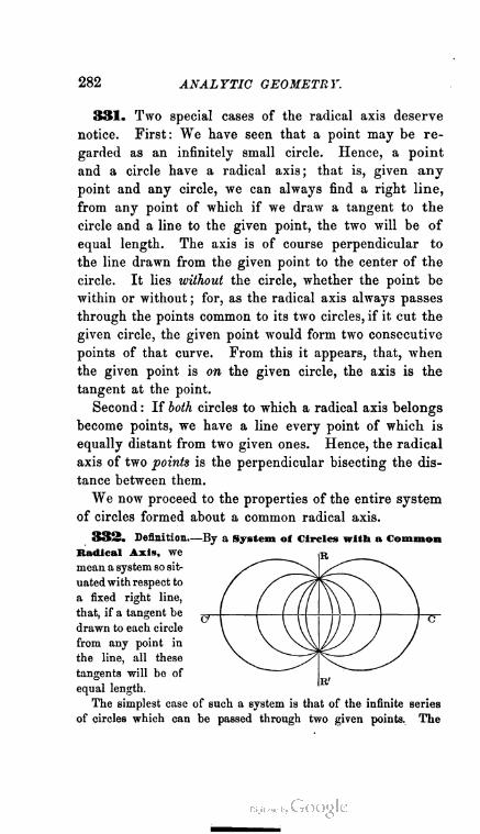
282 ANALYTIC GEOMETRY.
331. Two special cases of the radical axis deserve
notice. First: We have seen that a point may be re
garded as an infinitely small circle. Hence, a point
and a circle have a radical axis; that is, given any
point and any circle, we can always find a right line,
from any point of which if we draw a tangent to the
circle and a line to the given point, the two will be of
equal length. The axis is of course perpendicular to
the line drawn from the given point to the center of the
circle. It lies without the circle, whether the point be
within or without ; for, as the radical axis always passes
through the points common to its two circles, if it cut the
given circle, the given point would form two consecutive
points of that curve. From this it appears, that, when
the given point is on the given circle, the axis is the
tangent at the point.
Second : If both circles to which a radical axis belongs
become points, we have a line every point of which is
equally distant from two given ones. Hence, the radical
axis of two points is the perpendicular bisecting the dis
tance between them.
We now proceed to the properties of the entire system
of circles formed about a common radical axis.
332. Definition—By a System of Circles with a Common
Radical Axis, we
mean a system so sit
uated with respect to
a fixed right line,
that, if a tangent be
drawn to each circle
from any point in
the line, all these
tangents will be of
equal length.
The simplest case of such a system is that of the infinite series
of circles which can be passed through two given points. The
CIRCLES WITH COMMON AXIS. 283
diagram illustrates this case. Another is that of a series of circles
touching each other at a common point. The appearance of the
system when the two common points are imaginary, will be pre
sented farther on, in connection with the method of constructing
the system.
It follows directly from Art. 329, that all the centers of the system
lie on one right line at right angles to their radical axis.
333. Equation to any member of tbe System.—The equa
tion to any circle whose center lies on the axis of x, at a distance g
from the origin, may be written (Art. 134)
xl + y1 — 2gx — r2—g'2;
so that the circle will cut the axis of y in real or imaginary points
according as r2 —g1 is positive or negative, the quantity Vr2— g1
representing half the intercept on the axis of y. Hence, if in the
system of circles with a common radical axis, the common line of
centers be taken for the axis of x; and the common radical axis for
the axis of y : by putting k = the arbitrary distance of the center
from the origin, and eP= constant = r2 — k2, we may write the equa
tion to any member of the system
x2 + y2 — 2kx = d2;
and the corresponding system will cut the radical axis in real or
in imaginary points according as c-2 is positive or negative.
Corollary,—Hence, To trace the system from the equation, assume
different centers corresponding to arbitrary values of k, and from them,
with radii in each case equal to l/k2 ± (J2, describe circles.
334. The Ortbogonal Circle.—From the definition of the
system (Art. 332), it follows that the locus of the point of contact
of the tangent drawn from any point in the common radical axis
to any member of the system, is a circle. Since, then, the corre
sponding tangents of the system are all radii of this circle, tangents
to this circle at the points where it cuts the several members of the
system will be perpendicular to the respective tangents of the system.
In other words, the circle in question cuts every member of the
system at right angles,* and may therefore be called the orthogonal
circle of the system.
• The angle between two curves is the angle contained by their re
spective tangents at the point of intersection.
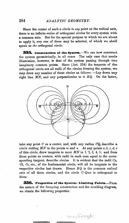
284 ANALYTIC GEOMETRY.
Since the center of such a circle is any point on the radical axis,
there is an infinite series of orthogonal circles for every system with
a common axis. But for the special purpose to which we are about
to apply it, any one of these may be selected, of which we shall
speak as the orthogonal circle.
335. Construction of the System.—We can now construct
the system geometrically, in all cases. The only case that needs
illustration, however, is that of the system passing through two
imaginary common points. Since (Art. 334) the tangents of the
orthogonal circle are all radii of the circles forming the system, we
may draw any number of these circles as follows : —Lay down any
right line MN, and any perpendicular to it HQ. On the latter,
take any point C as a center, and, with any radius CQ, describe a
circle cutting MN in the points m and n. At any points a, b, c, d, e
of this circle, draw tangents to meet MN in 1, 2, 3, 4, 5; and from
these points as centers, with radii in each case equal to the corre
sponding tangent, describe circles. It is evident that the radii Ca,
Cb, Ce, etc., of the fundamental circle, will all be tangents to the
respective circles last drawn. Hence RQ is the common radical
axis of all these circles, and the circle C-Qmn is orthogonal to
them.
336. Properties of the System: Limiting Points.—From
the nature of the foregoing construction and the resulting diagram,
we obtain the following properties-
PONCELET'S LIMITING POINTS. 285
I. The circles of a system having two imaginary common points,
in which the orthogonal circle cuts the line of centers in two real
points m and n, exist in pairs : to every circle on the right of the
radical axis, corresponds an equal one on the left, with an equally
distant center.
II. In a system of this character, the center of no circle can lie
nearer to the radical axis than m or n. For the radius of the vari
able member of the system continually diminishes as the tangent
of the orthogonal circle advances from Q toward m and n, and at
m and n it vanishes.
III. But the center of a member of the system may be as remote
from the radical axis as we please. For the tangents of the orthog
onal circle at Q meet the line of centers at infinity.
IV. Hence, the points m and n, and the axis RQ form the inferior
and superior limits of the system; in short, are the corresponding
limiting members of it : m and n being equal infinitesimal circles at
equal distances from the axis, and the axis itself being the resultant
of two coincident circles having equal infinite radii.
V. The circle C-Qmn is drawn in the diagram to cut MN in real
points ; but if the student will draw a new diagram, in which C- Qmn
fails to cut MN, he will find that the circles of the resulting system
all cut each other in two real points on the line HQ. Hence, a
system of circles with a common radical axis intersect each other
in two real or imaginary points, according as the limiting points m
and n are imaginary or real.
VI. The limiting points m and n are by construction equally
distant from every point in if Q. Moreover, every orthogonal circle
is described from some point in HQ, and cuts every member of the
system at right angles. Hence every orthogonal circle passes through
the limiting points. That is, The orthogonals of any system of circles
with a common radical axis, form a complemental systerh, whose radical
axis is the line joining the centers of the conjugate system.
VII. Hence, if a system of circles intersect in two real points,
the conjugate system of orthogonal circles will intersect in two
imaginary ones; and reciprocally.
337» The Limiting; Points by Analysis.—If a system of
circles cut its radical axis in two imaginary points, the equation to
any member of the system (Art. 333) is
x>+y* — 2kx=— <31 (1),

286 ANALYTIC GEOMETRY.
in which <52 is constant for the whole system, while k varies for each
different member. Xow — d~* = r2 — & . \ r = V Ul — o' : therefore
r vanishes when k = ± &, and becomes imaginary when k < 6 or
> — S. Hence, the two points (y = 0, x = <J) and (y = 0, a: = — <5)
are the infinitesimal circles which we have called the limiting points
of the system ; for we have just shown that they have the property
of Art. 336, II, and they are represented (Art. 61, Rem.) by the
equation
(x=F<5)' +y*= 0; that is, x> + y' =F2fa = — <J*
which conforms to the type of (1).
To exhibit the singular nature of these limiting points, we will
now develop one more property of the system to which they belong.
The equation to any of its members may be thrown into the form
(x-A)» + y» = r«.
Hence, (Art. 305, Cor.,*) the polar of any point x'y', with respect
to any member of the system, will be represented by
x'x + y'y + <SJ -A (x + aT) = 0 (2).
Now (Art. 108) the line denoted by (2) passes through the inter
section of the two lines i/x + y/y + (52 = 0 and x + x'=0, whatever
be the value of k. Therefore, 1/ the po/ars of a given point be taken
with respect to the whole system of circles having a common radical axis,
they will all meet in one point.
Suppose, then, that x'y' be either of the limiting points. The
polar will then become
x = =F S (3).
Hence, The polar of either limiting point is a line drawn through the
other at right angles to the line of centers, and is therefore absolutely
fixed, for the whole system.
II. TWO CIRCLES WITH A COMMON TANGENT.
338. The problem of constructing a common tangent
to two given circles (which properly belongs to Deter-
* The student will remember that the equations to the tangent and polar
of the Circle are identical in form.

CIRCLES WITH COMMON TANGENTS. 287
minate Geometry, and which we solved under that head
on pp. 18—21) leads to some important results when
treated by the methods of Indeterminate Geometry. A
few of these, we shall now present.
33©. The problem, as coming within the sphere of pure
analysis, consists in finding co-ordinates of contact such that the
corresponding tangent may touch both circles. Suppose, then, that
the equations to the two circles are
(x-gy + (y-fy = r' OS),
The equation to a tangent of S will then be (Art. 305, Cor.)
(x' -g)(x-g) + (,/ -/ ) (y _/)= ;
and our problem is, so to determine x'y" that this line may also
touch S'.
In settling what condition x'y' must satisfy in order that this
result may take place, it will be convenient to employ the auxiliary
angle mentioned in Art. 307. Let 0 = the inclination of the radius
through x'y': then will x" —g = r cosd, and y' —/=rsinS. The
equation to the tangent of S may therefore be written
x cos 0 + y sin 8 = g cos 6 +/sin6 + r (1),
and, similarly, the equation to a tangent of S',
xcoay + y sin0'=i/cos0'+//sin0' + r/ (2).
Now (1) will represent the same line as (2), if the mutual ratios
of its co-efficients are the same as those of (2); that is, if simul
taneously
tan0 = tan<?',
(srcos 6»+/sine + r) cos W= (/ cos V +/sin V + r') cos 6.
The first of these conditions is satisfied either by 6'=8, or d'=n-\-6.
Combining the two, then, on both suppositions, we obtain
( g'-g) cos 6 + (/'-/) sin d = r - /,
(g'-g) cos d + (/'-/) sin 6 = r + S ;

288 ANALYTIC GiEOMETRY.
or, after replacing cos S and sin » by their values, and ' — ,r r
W-9) («'-*) + (/'-/) (/-/ ) = r (r-r') (a),
W-9) + (/'-/) (/-/) = r (r+O (b) ;
and we learn that if a;V satisfies either (a) or (b), the tangent of S
will touch <S". Since (a) arose from the supposition O'—d, that is,
from the supposition that the radii of contact in the two circles were
parallel, and lay
in the same direc
tion, a moment's
inspection of the
diagram will show
that, when (a) is
satisfied, the com
mon tangent is
direct, as MN;
while as (b) arose
from V= ?r + 0,
that is, from sup
posing the radii of contact parallel, but lying in opposite directions,
the corresponding common tangent must be transverse, as mn.
To find, then, the required points on S, at which if a tangent be
drawn, it will also touch S/, we merely eliminate between (S) and
either (a) or (b). Now the result of this elimination will be a quad
ratic ; hence, there are in all four tangents common to S and <S" :
two direct, and two transverse.
84©. The Chords of Contact.—Since the points of contact,
M and M', as we have just seen, both satisfy the condition (a), it
follows that
(/- g) {*-g) + (/'-/ ) (y -/) = r (r - ✓) (1 ),
is the equation to the chord of contact for the direct tangents. Similarly,
(/-g) («-*) + (/'-/) (y-/)=r(r + K) (2),
is the equation to mm', the chord of contact for the transverse tangents.
Corollary—If the origin be transferred to the center of S, g andf
will vanish, and the chords of contact will be represented by
g'x +f'y = r (r q= /).
If the axes be now revolved until the line of centers becomes the
CENTERS OF SIMILITUDE. 289
axis of x, f will vanish, and the equation assume the form x =
constant. Hence, The chords of contact corresponding to common
tangents of two circles are perpendicular to the line of their centers.
311. Segments formed on the Line of Centers.—The
points O and C, in which the two direct and two transverse
common tangents have their respective intersections, are the poles
of (1) and (2) in Art. 340. In these, if we multiply by r, and then
divide by r — r/ and r-\-iy respectively, the co-efficients of x and y
(Art. 305, Cor.) will be the co-ordinates of O and C, diminished
by the co-ordinates of the center of S. We thus get
r -t- r r-t-r
r-t-r r -+- r
Now (Art. 95) these values satisfy the equation to the line of centers,
and show (Art. 52) that x'y' divides the distance between gf and
g'f in the ratio of r and r/. Hence, Common tangents of two circles
intersect on the line of their centers, and divide the distance between
those centers in the ratio of the radii.
342. Centers of Similitude.—If the common tangent be made
the initial line, and either O or C be taken for the pole, the polar
equation to the circle S (Art. 138) may be written
, _rcos(0 — a) r2cos2<z .ft2 -2 i '- ft -\ r-^— =0,
sin a sin a
by merely substituting for d its value r : sin a. Hence, for the circle S,
r f cos (ft — a) ± l/cos2 (t> — a) — cos'2 a \ft — ■ ■
sin o
Similarly, for the circle S/, we get
T* { COS (ff — a) ± l/cos2 (H — a) — cos'2 a \ft —■ ■ ■
sin a
Therefore, ft : ft : : r : t/.
Now these vectors of <S' and S/ are the segments formed by the two
circles on any right line drawn through O or C. Hence, All right
lines drawn through the intersection of the common tangents of two circles
are cut similarly by the circles, namely, in the ratio of the radii.
Remark—On account of this property, the points in which the
common tangents intersect are called centers of similitude.

290 ANALYTIC GEOMETRY.
343. Axis of Similitude.—This name is given to a certain
right line whose relation to three circles we will now develop.
Let gf, g'f, g"f" be the centers of any three circles, and r,
r" their radii. The co-ordinates of the external center of similitude
for the first and second (Art. 341) will then be
rg/— r'g rf —iJf
r — r' ' » r-r'
those of the corresponding center for the second and third,
r'g"— r"g' , ff"—>i"f
0);
7f:r— r" r'—r"
and those of the corresponding center for the third and first,
^,= r"g-rg" „_r"f-rf"
(2);
(3).
Now, if we make the necessary sub
stitutions and reductions, we shall find
that (1), (2), (3) satisfy the condition
of Art. 112. Hence, Any three homolo
gous centers of similitude belonging to
three circles lie on one right line, called
the AXIS OF SIMILITUDE.
Corollary.—If two circles touch each
other, one of their centers of similitude
becomes the point of contact. Hence,
If in a group of three cirqles the third
touches the other two, the line joining
the points of contact passes through a
center of similitude of the two.
Remark—The homologous centers of
similitude are either all three external,
as in the diagram, or else two internal
and the third external. Corresponding
to the latter case, there will of course be three different axes of
similitude; making in all four such axes for every group of three
circles.
THE CIRCLE IN THE ABRIDGED NOTATION.
344. We ^have room for only a few examples of the
uses to which this notation can be advantageously applied

CIRCLE IN ABRIDGED NOTATION. 291
in the case of the Circle. The illustrations given will
afford the beginner some further insight into the method,
and the reader who desires fuller information must con
sult the larger works to which we have already referred
in connection with this subject.
345. Since a, ft, y are the perpendiculars dropped from any
point P to the three sides of a triangle, it is evident that the
function
fty sin A -f ya sin B + aft sin C
denotes (Trig., 874) the double area of the triangle formed by
joining the feet of those perpendiculars; for the angle A, included
between the sides ft and y, will be either the supplement of the
angle between the perpendiculars ft and y, or else equal to it: and
so, also, of the angles B and C. Now (Art. 236) if the point P be
on the circumference of the circumscribed circle,
we have \ /
fty sin A-\-ya sin B + aft sin C= 0 ;/ /MY j X
that is, the triangle contained between the feet / / \\ \
of the perpendiculars from P vanishes, and we \ / \j \ I
obtain the following theorem : The feet of the A\~ S\/
perpendiculars droppedfrom any point in a circle
upon the sides of an inscribed triangle lie on one
right line.
34G. The equation to the circle circumscribed about a triangle
may, by factoring, be written
y(a sin B + ft sin A) + aft sin C=0:
which shows that the line a sin B + ft sin A meets the circle on the
line a, and also on the line ft; since, if a sin B + ft sin A = 0 in
the above equation, we get aft = 0, a condition satisfied by either
a = 0 or ft = 0. But the only point in which either a or ft meets
the circle is their intersection : hence a sin B + ft sin A is the tangent
of the circle at aft. Now (Ex. 8, p. 222) a sin A+ftsin B is the parallel
to the base of the triangle, passing through its vertex; and (Ex. 6,
p. 222) this parallel, and therefore the base, has the same inclina
tion to a or ft as the tangent a sin B + ft sin A has to ft or a. Hence,
the tangent of the circumscribed circle, at the vertex of a triangle.
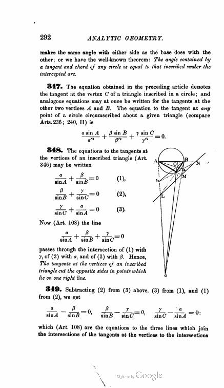
292 ANALYTIC GEOMETRY.
makes the same angle with either side as the base does with the
other; or we have the well-known theorem: The angle contained by
a tangent and chord of any circle is equal to that inscribed under the
intercepted arc.
347. The equation obtained in the preceding article denotes
the tangent at the vertex C of a triangle inscribed in a circle ; and
analogous equations may at once be written for the tangents at the
other two vertices A and B. The equation to the tangent at any
point of a circle circumscribed about a given triangle (compare
Arts. 236; 240, II) is
a sin A /3 sin B y sin C n
a" 1 /F3 *~ ■/*
348. The equations to the tangents at
the vertices of an inscribed triangle (Art
346) may be written
£b + ^c=» <2>-
fife + ah-0 (3)-
Now (Art. 108) the line
sin.4 sin.fi sinC
passes through the intersection of (1) with
7, of (2) with a, and of (3) with /?. Hence,
The tangents at the vertices of an inscribed
triangle cut the opposite sides in points which
lie on one right line.
349. Subtracting (2) from (3) above, (3) from (1), and (1)
from (2), we get
_2 L. = Q A >l = 0 JL-lf- =o-sin.4 sin.fi ' sin.fi sinC ' sinC sin^
which (Art. 108) are the equations to the three lines which join
the intersections of the tangents at the vertices to the intersections
CIRCLE IN ABRIDGED NOTATION. 293
of the sides. Hence, (Art. 114,) The lines which join the vertices
of a triangle to those of the triangle form.ed by drawing to its circum
scribed circle tangents at its vertices, meet in one point.
Bemark The theorems of the last two articles, which are illus
trated in the diagram, are evidently a particular case of homology
(Art. 327) due to a pair of conjugate triangles.
350. Radical Axis in Trilinears.—The equations
to any two circles, in the abridged notation, (Arts. 236,
237) are
sin A sin B sin C . a , N n
___ 4- _— -| — -f M (la + mp + nf) = 0,
sin A , sin B , sin C . . ,a , , ■. A1 1 f- M (l a + m'p -f- n'y) = 0.
Hence, their radical axis, S—S', is denoted by
la + mft + ny= Va + m'jj + n'y.
Corollary.—The radical axis of any circle and the
circle circumscribed about the triangle of reference, is
represented by
la + ni/3 ~\- ny — 0.
EXAMPLES ON THE CIRCLE.
1. Find the intersections of the line 4.r+3y = 35e with the
circle
(x— c)2 + (y— 2c)2= 25cs.
Also, the tangents from the origin to the circle a'+y2—6x—2y+8=0.
2. Show that the equation to any chord of a circle may be
written
{X-x>)(x-x") + (y-y'){y-y") = x> + tf- r2,
the origin being at the center, and x'y', x"y" being the extremities
of the chord.
3. Find the polar of (4, 5) with respect to x2+ y1— 3x — 4y = 8,
and the pole of 2x + Zy= 6 with respect to (x—1)2+ {y—2)2= 12.
294 ANALYTIC GEOMETRY.
4. Prove that the condition upon which Ax + By + C= 0 will
touch the circle (x — g)'1 + (y —fY = r* is
Ag±fy± C
5. Find the length of the chord common to the two circles
(x - af + (y - py = r1, (x - PY + (y- a)2 = r».
Also, the equations to the right lines which touch x2 + y2 = '"2 at
the two points whose common abscissa is 1.
6. Find the equation to the circle of which y = 2x + 3 is a
tangent, the center being taken for the origin.
7. Prove that the bisectors of all angles inscribed in the same
segment of a circle pass through a fixed point on the curve.
8. Given the hypotenuse of a right triangle : the locus of the
center of the inscribed circle is the quadrant of which the given
hypotenuse is the chord.
9. Given two sides and the included angle of a triangle : to
find the equation to the circumscribed circle.
10. The locus of a point from which if lines be drawn to the
vertices of a triangle, their perpendiculars through the vertices will
meet in one point, is the circle circumscribed about the triangle.
11. If any chord be drawn through a fixed point on the diameter
of a circle, and its extremities joined to either end of the diameter,
the joining lines will cut from the tangent at the other end, portions
whose rectangle is constant. [See Art. 137.]
12. The locus of the intersection of tangents drawn to any circle
at the extremities of a constant chord is a concentric circle. [See
Art. 307.]
13. If a chord of constant length be inscribed in a given circle,
it will always touch a concentric circle.
14. If through a fixed point 0 any chord of a circle be drawn,
and OP be taken an harmonic mean between its segments OQ,
OQf, the locus of P will be the polar of O.
15. If through any point O of a circle, any three chords be
drawn, and on each, as a diameter, a circle be described, the three
circles which thus meet in O will meet in three other points, lying
on one right line.
EXAMPLES ON THE CIRCLE. 295
16. If several circles pass through two fixed points, their radical
axes with a fixed circle will pass through a fixed point.
[This example may be best solved by means of the Abridged Notation,
but can be done very neatly without it.]
17. Form the equation to the system of circles which cuts at
right angles any system with a common radical axis, and prove,
by means of it, that every member of the former system passes
through the limiting points of the latter.
18. IfPQbe the diameter of a circle, the polar of P with respect
to any circle that cuts the first at right angles, will pass through Q.
19. The square of the tangent drawn to any circle from any point
on another is in a constant ratio to the perpendicular drawn from
that point to their radical axis.
20. If a movable circle cut two fixed ones at constant angles, it
will cut at constant angles all circles having the same radical axis
as these two.
[First prove that the angle 0 at which two circles cut each other, is
determined by the formula
D2=B2 + r2-2Jtr cos <p,
in which R, r are the radii of the circles, and D the distance between
their centers.]
21. Find the equations to the common tangents of the two
circles
rf+y2 — 4x — 2y + 4 = 0, x* + f + 4x + 2y— 4 = 0.
What is the equation to their radical axis?
22. If a movable circle cut three fixed ones, the intersections of
the three radical axes will move along three fixed right lines which
meet in one point.
23. The radical axis of any two circles that do not intersect,
bisects the distances between the two points of contact correspond
ing to each of the four common tangents.
24. If through a center of similitude belonging to any two circles,
we draw any two right lines meeting the first circle in the points
R and R', S and S' respectively, and the second in r and r', s and
s' : then will the chords RS and rs, R'S' and rV, be parallel ; while
RS and rV, R'S' and rs, will each intersect on the radical axis.
An. Ge. 28.
290 ANALYTIC GEOMETRY.
25. Find the trilinear equation to the circle passing through the
middle points of the sides of any triangle, and prove that this circle
passes through the feet of the three perpendiculars of the triangle,
and bisects the distances from the vertices to the point in which
the three perpendiculars meet. [This circle is celebrated in the
history of geometry, and, on account of passing through the points
just mentioned, is called the Nine Points Circle.]
Find, also, the radical axis of this and the circumscribed circle.
GHAPTER THIRD.
THE ELLIPSE.
I. The Curve referred to its Axes.
351. We may most conveniently begin the discussion
of the Ellipse by means of the equation which we obtained
in Art. 147, namely,
-4-^-1a2 + ¥ - A'
At a later point in our investigations, we shall refer the
curve to lines which have a relation to it more generic
than that of the two known as the axes (Art. 146), which
give rise to the equation just written.
THE AXES.
352. If in the above equation we make y = 0, we
shall obtain, as the intercept of the curve upon the
transverse axis,
x = ±a (1);

PROPERTIES OF THE ELLIPSE. 297
and, making x= 0, we get, for the intercept upon the
conjugate axis,
y = ±b (2).
Comparing (1) and (2), we see that the curve cuts both
axes in two points, and that in each case these two points
are equally distant from the focal center, which (Art. 147)
was taken for the origin. Hence we have
Theorem I.—The focal center of any ellipse bisects the
transverse axis, and also the conjugate.
Corollary.—We must therefore from this time forward
interpret the constants a and b in the equation
*- + t = 1
a2 + b>
as respectively denoting half the transverse axis and
half the conjugate axis.
Remark—This theorem follows, of course, directly from that of
Art. 149. We have purposely developed it by a separate analysis,
however, in order that the student may see the consistency of the
analytic method.
353. If in the equation of Art. 147, which may be
written
y = ±-Va2-x2,
we suppose x > a or < — a, the corresponding values
of y are imaginary; so that no point of the curve is
farther from the origin, either to the right or to the left,
than the extremities of the transverse axis. Now (Art.
147), for the distance from the origin to either focus,
we have
c* = a2-&2.
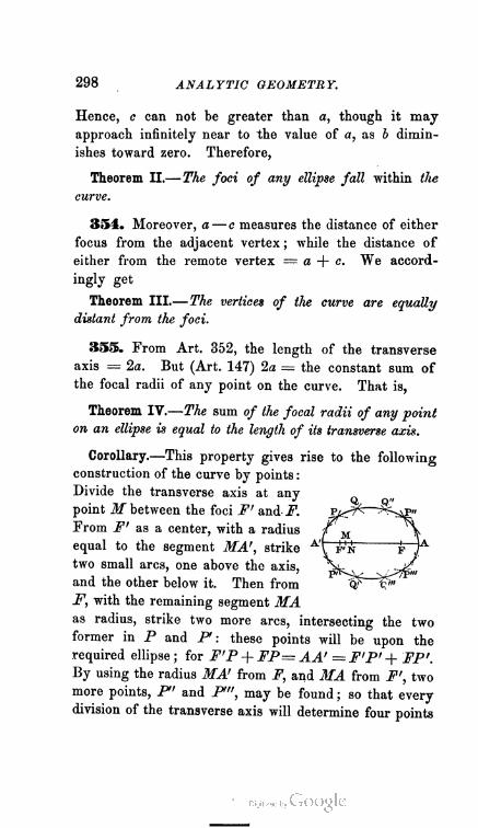
298 ANALYTIC GEOMETRY.
Hence, c can not be greater than a, though it may
approach infinitely near to the value of a, as b dimin
ishes toward zero. Therefore,
Theorem II.— The foci of any ellipse fall within the
curve.
354. Moreover, a — c measures the distance of either
focus from the adjacent vertex ; while the distance of
either from the remote vertex = a + c. We accord
ingly get
Theorem III.—The vertices of the curve are equally
distant from the foci.
355. From Art. 352, the length of the transverse
axis = 2a. But (Art. 147) 2a = the constant sum of
the focal radii of any point on the curve. That is,
Theorem IV.—The sum of the focal radii of any point
on an ellipse is equal to the length of its transverse axis.
Corollary.—This property gives rise to the following
construction of the curve by points :
Divide the transverse axis at any
point M between the foci F' and F.
From F' as a center, with a radius
equal to the segment MA', strike A'
two small arcs, one above the axis,
and the other below it. Then from
F, with the remaining segment MA
as radius, strike two more arcs, intersecting the two
former in P and P : these points will be upon the
required ellipse ; for F'P + FP= AA' = F'P' + FP'.
By using the radius MA' from F, and MA from F', two
more points, P" and P", may be found ; so that every
division of the transverse axis will determine four points
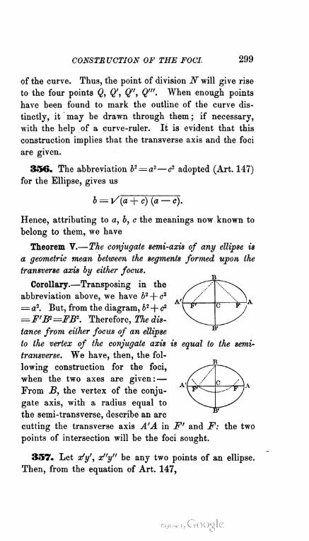
CONSTRUCTION OF THE FOCI. 299
of the curve. Thus, the point of division 2V will give rise
to the four points Q, Q', Q", Q'". When enough points
have heen found to mark the outline of the curve dis
tinctly, it may be drawn through them ; if necessary,
with the help of a curve-ruler. It is evident that this
construction implies that the transverse axis and the foci
are given.
356. The abbreviation 62=a2— c2 adopted (Art. 147)
for the Ellipse, gives us
b = VJa + c) (a — c).
Hence, attributing to a, b, c the meanings now known to
belong to them, we have
Theorem V.—The conjugate semi-axis of any ellipse is
a geometric mean between the segments formed upon the
transverse axis by either focus.
Corollary.—Transposing in the
abbreviation above, we have b2-{-c2
= a2. But, from the diagram, b2 -\- c2
=F'B2=FB2. Therefore, The dis
tance from either focus of an ellipse
to the vertex of the conjugate axis is equal to the semi-
transverse. We have, then, the fol
lowing construction for the foci,
when the two axes are given:—
From B, the vertex of the conju
gate axis, with a radius equal to
the semi-transverse, describe an arc
cutting the transverse axis A'A in F' and F: the two
points of intersection will be the foci sought.
357. Let x'y', x"y" be any two points of an ellipse.
Then, from the equation of Art. 147,

300 ANALYTIC GEOMETRY.
*2(a2-x% y"2=bl(a2-x"2) (1);
|>-y"), x"2=^{b2-y"2) (2).
Dividing the first equation of (1) by the second, we get
y 12 : y"2 : : (a + x') (a — x') : {a + x") (a — x").
By a like operation in (2), we obtain
x'2 : x"2 : : (b + y') (b - y') : (b + y") (b - y").
Now a + x', a — xf are evidently the segments formed
by y' upon the transverse axis, and a + x", a — x" are
those formed by y". Similarly, b-\-y', b — y' are the
segments formed by X* upon the conjugate axis, and
b + y", b — y" those formed by x". Hence,
Theorem VI.— The squares on the ordinates drawn to
either axis of an ellipse are proportional to the rectangles
under the corresponding segments of that axis.
Corollary.—If in the first expression of (1) we make
x' = ± c, we get
2/'2 = ^(«2-*2)-
But a2— c2 = b2. Hence, after re- A'
ductions,
y>= FP or F'F = - .a a
Now, either of the double ordinates that pass through
the foci, PQ or PQ', is called the latus rectum of the
ellipse to which it belongs. Hence,
latus rectum = — = •
a 2a
yn=
x'2=
CIRCUMSCRIBED CIRCLE. 301
That is, The latus rectum of any ellipse is a third propor
tional to the transverse axis and the conjugate.
358. The equation to the Ellipse (Art. 147) may be
thrown into either of the forms
y2 b2 x2 a2
{a + x) (a-x) = a2 ' (b + y)(b- y) = b2 '
Hence, since a ratio is not altered when both its terms
are multiplied by the same number,
Theorem VII.—The squares on the axes of any ellipse
are to each other as the rectangle under any two segments
of either is to the square on the ordinate which forms the
segments.
Note.—It may be worth while to observe, in passing, that, in this
theorem and the one of Art 357, the word ordinate has been used
in a wider setose than we originally assigned to it. We shall fre
quently have occasion to employ it in this larger meaning, of a line
drawn to either axis of co-ordinates parallel to the other.
359. The equation to the Ellipse being put into the
form
»■ (1),
the equation to the circle described on the transverse
axis as a diameter (Art. 161) will be
f = a2 — xi (2).
Hence, supposing the x of (1) and (2) to become iden
tical, we get
ye: yc::b : a.
That is to say,
Theorem VIII.—The ordinate of any ellipse is to the
corresponding ordinate of the circumscribed circle, as the
conjugate semi-axis is to the semi-transverse.

302 ANALYTIC GEOMETRY.
Corollary 1.—By similar reasoning, we should find
that the abscissa of an ellipse is to the corresponding
abscissa of the inscribed circle, as the transverse semi-axis
is to the semi-conjugate. When the axes are given, we
may therefore construct the curve by either of the
following methods :
First: Describe circles upon the
given axes A'A, B'B. At any point
Mof the transverse axis, erect a per
pendicular, and join the point Q, in
which it meets the outer circle, with
the common center C. Through It,
in which QC cuts the inner circle,
draw MP at right angles to the con
jugate axis : the point P, in which MP cuts MQ, will
be upon the required ellipse. For, by similar triangles,
MP : MQ :: CM : CQ ::b : a.
Second : Suppose PS to be a ruler whose length = OA.
From the end P, lay off upon it PV= OB. Set the end
S against the conjugate axis, say at some point below C,
and rest the point V upon the transverse axis, say to the
right of C. Move the ruler so that S and V may slide
along the axes : the extremity P will describe an ellipse.
For, if MPQ be drawn through P perpendicular to CA,
and QC be joined, the latter will be equal and thence
parallel to the ruler PS, and we shall have the proportion
MP-.MQ:: PV : PS::b: a.
The second of these methods constitutes the principle
of the so-called elliptic compasses— an instrument used
for describing ellipses, and consisting of two bars, A'A,
B'B, fixed at right angles to each other, along which
a third, PS, slides freely upon two points, £ and V,
whose distance apart is constant. [See Ex. 6, p. 167.]
i

ECCENTRICITY. LINEAR EQUATION. 303
Corollary 2.—We are now enabled to interpret the
abbreviation
adopted in Art. 150. In the first place, since a2— b2= c2,
we learn that e is the ratio which the distance from the
center to either focus of an ellipse bears to its transverse
semi-axis. But (Art. 161) a circle is an ellipse in which
c — 0, or in which, therefore, a = b. In any circle, then,
the ratio e is equal to zero. Hence, if we compare ellipses
having a common transverse axis =2a with their common
circumscribed circle, it is evident (since e will increase as
the conjugate semi-axis b diminishes from the maximum
value a toward zero) that e may be taken to measure
the deviation of any of these ellipses from the circum
scribed circle. For this reason, the ratio e is called the
eccentricity of the ellipse to which it belongs.
The eccentricity of any ellipse evidently lies between
the limits 0 and 1. In fact the name ellipse (derived from
the Greek iXXdzeiv, to fall short) may be taken as signi
fying, that, in this curve, the eccentricity is less than unity.
Since e increases as b diminishes, it is evident that the
greater the eccentricity, the flatter will be the correspond
ing ellipse.
360. The distance of any point on an ellipse from
either focus, may be expressed in terms of the abscissa
of the point. For, putting p to denote any such focal
distance, we have (Art. 147)
pi = (c ± xf + y\
But, from the equation to the Ellipse,
An. Ge. 29.

804 ANALYTIC GEOMETRY.
Substituting and reducing, and remembering (Art. 151)
that b2 + c2 = a2, d2 — b2 = aV, and c = ae, we get
/£> = a ± ear,
in which the upper sign corresponds to the left-hand
focus, and the lower sign to the right-hand one. Hence,
since p and x are of the first degree,
Theorem IX.—The focal radius of any point on an
ellipse is a linear function of the corresponding abscissa.
Remark.—The expression just obtained is accordingly
known as the Linear Equation to the Ellipse.
361. The form of the Ellipse is already familiar to
the student, from the method of generating it given in
Art. 145. Its appearance shows, or at least suggests,
that it is an oblong, closed curve, continuous in extent,
and symmetric to both of its axes. But it may be inter
esting, at this point, to show how we might have discovered
each of these peculiarities of form from the equation itself,
without the aid of any drawing.
I. The curve is oblong. For, no matter where we take it between
its two limiting cases, the Point and the Circle, in its equation
b (since it is equal to Va.1— c1) must be less than a; that is, the
conjugate axis must be less than the transverse.
II. It is closed, i. e., limited in the directions of both axes. For,
if we suppose i>aor < — a, the corresponding values of y are
imaginary; and, if we suppose y~>b or < — b, the corresponding
values of x are imaginary.
III. It is continuous in extent. For, between the limits x = — a
and x = a, all the values of y are real.
IV. It is symmetric to both axes. For, corresponding to every
value of x between the limits — a and a, the two values of y are
numerically equal with opposite signs; and the same is true of the
values of x corresponding to any value of y between — b and b.

BISECTORS OF PARALLEL CHORDS. 305
DIAMETERS.
362. Equation to any Diameter.—We are re
quired to find the equation to the locus of the middle
points of any system of parallel chords in an ellipse.
Let xy be the variable point of this locus, 0' the common
inclination of the bisected chords, and x'y' the point in
which any chord of the system cuts the curve. Then
(Art. 101, Cor. 3)
x1 — x — I cos 0', y" — y — I sin 0'.
But x'y' is a point on the curve ; hence (Art. 147)
(x — I cos O'Y (y — lsm gQ2_,
a1 + b2
That is, to determine the distance I between xy and x'y',
we get
{a2 sin2 d' + b2 cos2 6') P—2 (a2y sin 0' + b2x cos 0') I
+ (b2x2 + ay—a262) = 0.
Now, xy being the middle point of any chord, the two
values of I must be numerically equal with opposite
signs. Therefore (Alg., 234, Prop. 3d) the co-efficient
of I vanishes, and we obtain, as the required equation,
y — x cot 0'.
Corollary.—Let 6 = the inclination of any diameter
to the transverse axis. The co-efficient of x in the
equation just found is equal (Art. 78, Cor. 1) to tan 0.
Hence, as the condition connecting the inclination of any
diameter with that of the chords which it bisects,
tan d tan 6' = = •
a2
306 ANALYTIC GEOMETRY.
363. The equation to any diameter conforms to the
type y = mx. Therefore (Art. 78, Cor. 5) we have
Theorem X.—Every diameter of an ellipse is a right
line passing through the center.
Corollary.—Since 0' in the foregoing condition is ar
bitrary, 6 is also arbitrary. Hence, the converse of this
theorem is true ; that is, Every right line that passes through
the center of an ellipse is a diameter.
364. If we eliminate between the equation to the
Ellipse and that of any diameter, the roots of the result
ing equation will be
a2sin#'x—~ v'(a2sin2<y' + b2 cosW) ''
which, it is evident, are necessarily real. Hence,
Theorem XI.—Every diameter of an ellipse cuts the
curve in two real points.
365. Length of any Diameter.—This is of course
double the radius vector given by the central polar equa
tion (Art. 150), namely,
9 1 — e2 cos2 1) '
Hence, given the inclination 0, the length of the corre
sponding diameter can at once be found.
366. From the preceding formula, it is evident that
the diameter is longest when 6 = 0, and shortest when
6 = 90°. That is,
Theorem XII.—In every ellipse, the transverse axis is the
maximum, and the conjugate axis the minimum diameter.
Remark.—For this reason, the transverse axis is called
the axis major, and the conjugate, the axis minor.

CONJUGATE DIAMETERS. 307
367. Moreover, since d enters the foregoing formula
by the square of its cosine, the value of p is the same for
6 and tz — 0. Hence,
Theorem XIII.—Diameters which make supplemental
angles with the axis major of an ellipse are equal.
Corollary.—The converse of this is also given by the
formula; so that, having the curve,
we can always construct the axes as
follows: —Draw any two pairs of
parallel chords, and, by means of A'
them, two diameters DC, D'C: their
intersection C (Art. 363) will be the
center. From C describe any circle cutting the curve
in four points P, Q, P, Q'. The diameters PF, QQ'
will then be equal, and, by the converse of the theorem
above, the two bisectors of the angles between them
will be the axes. These bisectors may be drawn most
readily by forming the chords PQ, QP' which subtend
the angles : they will be perpendicular to each other
(Art. 317, Cor.), and their parallels through C will be
the bisecting axes required.
368. Let d and 0' be the inclinations of any two
diameters to the axis major. Then the condition that
the first shall bisect chords parallel to the second (Art.
362, Cor.) is
b2tan 0 tan 0' = r, •
<r
But this is also the condition upon which the second
would bisect chords parallel to the first. Hence,
Theorem XIV.—If one diameter of an ellipse bisects
chords parallel to a second, the second bisects chords
parallel to the first.
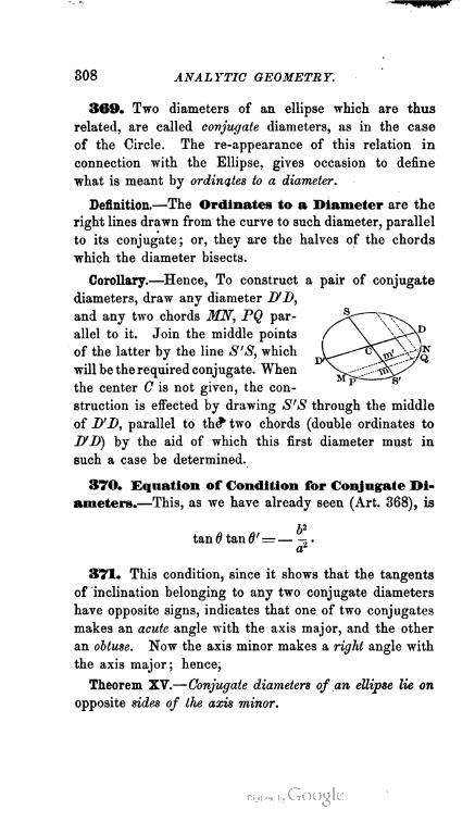
308 ANALYTIC GEOMETRY.
369. Two diameters of an ellipse which are thus
related, are called conjugate diameters, as in the case
of the Circle. The re-appearance of this relation in
connection with the Ellipse, gives occasion to define
what is meant by ordinates to a diameter.
Definition.—The Ordinate* to a Diameter are the
right lines drawn from the curve to such diameter, parallel
to its conjugate; or, they are the halves of the chords
which the diameter bisects.
Corollary.—Hence, To construct a pair of conjugate
diameters, draw any diameter ItD,
and any two chords MN, PQ par
allel to it. Join the middle points
of the latter by the line S'S, which
will be the required conjugate. When
the center C is not given, the con
struction is effected by drawing S'S through the middle
of D'D, parallel to the* two chords (double ordinates to
D'D) by the aid of which this first diameter must in
such a case be determined.
370. Equation of Condition for Conjugate Di
ameters.—This, as we have already seen (Art. 368), is
b2tan d tan 6' = ?, •
a1
371. This condition, since it shows that the tangents
of inclination belonging to any two conjugate diameters
have opposite signs, indicates that one of two conjugates
makes an acute angle with the axis major, and the other
an obtuse. Now the axis minor makes a rigid angle with
the axis major; hence;
Theorem XV.—Conjugate diameters of an ellipse lie on
opposite sides of the axis minor.

EXTREMITIES OF CONJUGATES. 309
372. Equation to a Diameter conjugate to a
Fixed Point.—For brevity, we shall say that a diam
eter is conjugate to a fixed point, when it is conjugate to
the diameter drawn through such point. If, now, x'y'
be any fixed point, the diameter drawn through it (Art.
95, Cor. 2) will be
y'x — x'y = 0 (1).
The equation to the conjugate will be of the form
y = x tan d' (2),
in which (Art. 370) tan 6' is determined by the condition
b2tan 0 tan 0' —
a2
But (1), tan 0 = y' : x1. Hence, the equation sought is
*te , vfy _ n
Corollary.—The equation to the diameter conjugate to
that which passes through the point (a, 0) is evidently
£= 0. But the diameter through (a, 0) is the axis major,
while x= 0 denotes the axis minor. Hence, The axes of
an ellipse constitute a case of conjugate diameters.
It is from this fact, that the axis minor derives its
name of the conjugate axis.
373. Problem.—Given the co-ordinates of the extremity
of a diameter, to find those of the extremity of its conjugate.
Let x'y' be the extremity of the given diameter. The
required co-ordinates, found by eliminating between the
equation of Art. 372 and that of the Ellipse, are
, au' bx'
b a
374. The expressions just obtained, transformed into the pro
portionsx0 ■■ y' : : a : b, a/ : yc : : a : b,
give us

310 ANALYTIC GEOMETRY.
Theorem XVI—The abscissa of the extremity of any diameter is to
the ordinate of the extremity of its conjugate, as the axis major is to
the axis minor.
375. Squaring the second expression of Art. 373,
adding y'2, and remembering that x'y' satisfies the equa
tion to the Ellipse, we find
Hence, in ordinary language, we have
Theorem XVII.—The sum of the squares on the ordinates
of the extremities of conjugate diameters is constant, and
equal to the square on the semi-axis minor.
Remark.—The student may prove the analogous prop
erty:—The sum of the squares on the abscissas of the
extremities of conjugate diameters is constant, and equal
to the square on the semi-axis major.
876. Problem.—To find the length of a diameter in
terms of the abscissa of the extremity of its conjugate.
Let a' be half the length required. Then, x'y' being the
extremity of a', we have (Art. 51, 1, Cor. 2) an = xn-\-y'2.
Substituting for x? and y1 from Art. 373, we get
n a2 i , & 2a
But xc and yc satisfy the equation to the Ellipse ; hence,
az c a2
Therefore (Art. 151), for determining the required length,
we have
a'2 = a2 — e2x2.
By a precisely similar analysis, we should find
b'2=a2— e2x'2.
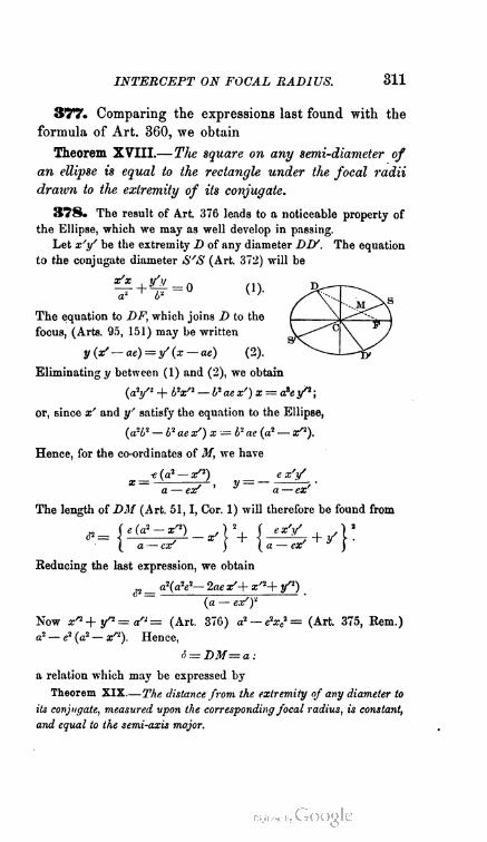
INTERCEPT ON FOCAL RADIUS. 311
STTo Comparing the expressions last found with the
formula of Art. 360, we obtain
Theorem XVIII.—The square on any semi-diameter of
an ellipse is equal to the rectangle under the focal radii
drawn to the extremity of its conjugate.
378. The result of Art. 376 leads to a noticeable property of
the Ellipse, which we may as well develop in passing.
Let x'y' be the extremity D of any diameter DW. The equation
to the conjugate diameter S'S (Art. 372) will be
¥ +*=° ('>•
The equation to DF, which joins D to the
focus, (Arts. 95, 151) may be written
y (3/ — ae) = y'(x — ae) (2).
Eliminating)/ between (1) and (2), we obtain
(ay2 + l>V2 — b2 ae x') x = a>e y* ;
or, since x' and y' satisfy the equation to the Ellipse,
(a%2 — b2 ae x') x -=b*ae (a2 — x'2).
Hence, for the co-ordinates of M, we have
■e (a2 — x/r) e x't/X = — 7^ , y — ■
a — ear a — ex'
The length of DM (Art. 51, 1, Cor. 1) will therefore bo found from
Reducing the last expression, we obtain
_ a!(aV- 2aex,+ x'2+ y'2)
° ~~ (a — ex'f
Now xn + y/2 = of2 = (Art. 376) s'-eV= (Art. 375, Rem.)
a2 — e2 (a2 — xn). Hence,
a = DM=a:
a relation which may be expressed by
Theorem XIX—The distance from the extremity of any diameter to
its conjugate, measured vpon the corresponding focal radius, is constant,
and equal to the semi-axis major.

312 ANALYTIC GEOMETRY.
379. Let V denote the length of the semi-diameter
conjugate to that whose extremity is x'y'. Then (Art.
51, I, Cor. 2) we shall have
V2 = x* + y?= (Art. 147) x? + ^ (a2-*,2).
Reducing, and applying the abbreviation of Art. 150,
we get
b'2 = b2+ e%\
Now (Art. 376) a'2 = a2— (?x*. Adding this expression
to the preceding, we find
a'2 + bn == a2 + b2,
giving us the following important property :
Theorem XX.—The sum of the squares on any two con
jugate diameters of an ellipse is constant, and equal to the
sum of the squares on the axes.
3S0. Angle between two Conjugates.—Let <p de
note the angle required. We shall then have <p — d'— d;
whence (Trig., 845, in)
sin (p = sin 6' cos 0 — cos d' sin 0.
But, putting a', V for the lengths of the semi-diameters,
and x'y', xcye for their extremities, we have
sin 6'— yc : V, cos d'= xc : V ;
cos 0 =■■ x1 : a', sin 0 = y1 : a'.
Hence, sin <p — - ^c ,,f — ;
ao'
or, substituting for xc and yc from Art. 373, and reducing,
5V2 + aV2sin 0 = -—— .
V ab.a'b'
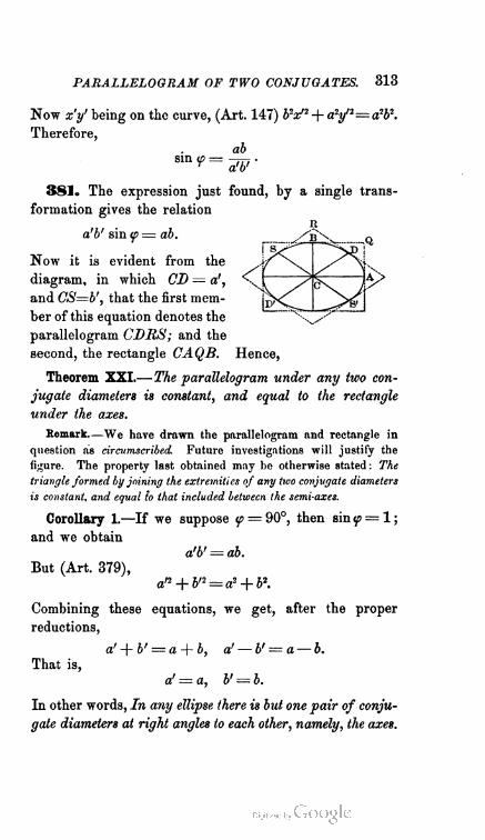
PARALLELOGRAM OF TWO CONJUGATES. 313
Now x'y' being on the curve, (Art. 147) &V2 + a2yn= a2b2.
Therefore,
ab
' a'b'
381. The expression just found, by a single trans
formation gives the relation
a'b' sin <p = ab.
Now it is evident from the
diagram, in which CD = a', *\
and CS—b', that the first mem
ber of this equation denotes the
parallelogram CDMS; and the
second, the rectangle CAQB. Hence,
Theorem XXI.—The parallelogram under any two con
jugate diameters is constant, and equal to the rectangle
under the axes.
Remark—We have drawn the parallelogram and rectangle in
question as circumscribed. Future investigations will justify the
figure. The property last obtained may be otherwise stated : The
triangle formed by joining the extremities of any two conjugate diameters
is constant, and equal to that included between the semi-axes.
Corollary 1.—If we suppose ip = 90°, then sin f = 1 ;
and we obtain
a'b' ab.
But (Art. 379),
av+b'2 = a2 + b\
Combining these equations, we get, after the proper
reductions,
a' + b' = a + b, a' — b' = a— b.
That is,
a' — a, b' = b.
In other words, In any ellipse there is hit one pair of conju
gate diameters at right angles to each other, namely, the axes.

314 ANALYTIC GEOMETRY.
Corollary 2.—From the formula (Art. 380), <p is obvi
ously greatest * when a'b' is greatest. But since a'2 -f- b'2
is constant, the rectangle a'b' has a constant diagonal,
and is therefore greatest when a' = b'. Hence, The
inclination of two conjugate diameters is greatest when
the diameters are of equal lengths.
382. The diameters corresponding to the condition
a'= b' may be appropriately termed the equi-conjugate
diameters of the ellipse to which they belong. Now
(Art. 367, Cor.) for the case of equi-conjugates,
tan 6' =— tan 0 ;
hence (Art. 370), for the inclinations of the equi-conju
gates to the axis major,
, M B l
tan 0 = ± - •
aA'
If we form the rectangle of the
axes, LMNR, it is evident that the
first of the two values just found,
corresponds to the angle ACL; and the second, to the
angle ACM. Hence,
Theorem XXII.—The equi-conjugates of an ellipse are
the diagonals of the rectangle contained under its axes.
Corollary.—It follows directly from this, that an ellipse
can have but one pair of equi-conjugates. In this case,
(Art. 379,) 2a'2 = a2 + b2; so that (Art. 380)
2ab
383. We shall find hereafter that the two lines just
brought to our notice have a striking significance with
• Tho angle ip is supposed to be that angle between two conjugates
which is not acute.

TANGENT OF THE ELLIPSE. 315
respect to the analogy between the Ellipse and the
Hyperbola. They in fact foreshadow the two remarka
ble lines known as the asymptotes of the latter curve,
which, though still the diagonals of the rectangle formed
upon its axes, meet it only at infinity.
THE TANGENT.
384. Equation to any Chord.—Let x'y\ x"y" be
the extremities of any chord in an ellipse : then (Art. 147)
6V2 + a2y'2 = b2x"2 + a2y"2.
Hence, after transposing and factoring,
y"—y' _ x'+x"
x"—a/ tf'y'+y" W'
Now the equation to the chord (Art. 95) must be of the
form
y — y' _ y"—y' _
x — x' x"— x1
Substituting from (1) for the second member, the required
equation is
y — y' b2 x' +
x — a/ a2 y'-\-y"
385. Equation to tbc Tangent.—Suppose the
two points in which the chord cuts the curve to become
coincident : then, in the preceding expression, x" = x1,
y" — y' ; and the required equation to the tangent, in
terms of the point of contact x'y', is
y — y' b2 x' .'
x — x' a2 y' '
or, by clearing of fractions and remembering that x' and
y' satisfy the equation to the curve,
x'x y'y

316 ANALYTIC GEOMETB.Y.
3S6. Condition that a Right Line shall touch
an Ellipse.—Eliminating y between the line y=mx-\- n
and the ellipse ,2
we obtain, as the equation determining the intersections
of the line and the curve, the quadratic
(wiV + V) x2 + 2ma2nx + a2 (n2— b2) = 0.
The condition that this may have equal roots is .
(ma2n)2 = a2 (n2 — ¥) (m2a2 +„ b2).
Hence, after the necessary reductions, the required con
dition of tangency is
n = /mV+ 4*.
Corollary.—Every right line, therefore, whose equation
is of the form
y= mx + VmV + b2
is a tangent to the ellipse whose semi-axes are a and b.
This expression, like the corresponding one belonging to
the Circle (Art. 306, Cor.), affords singularly rapid solu
tions of problems which do not involve the point of contact ;
and for this reason is called the Magical Equation to the
Tangent.
387. Tne Eccentric Angle.—If the ordinate of any point P
on an ellipse be produced to meet the cir
cumscribed circle in Q, and Q be joined to
the center C, the angle QCM is called the
eccentric angle of the point P. We intro
duce it here, because it serves the impor
tant purpose of expressing the position of
any point on an ellipse in terms of a single
variable : a purpose sometimes especially
useful in connection with the equation to a chord or a tangent.
The eccentric angle is usually denoted by <j>.
/B k JV s
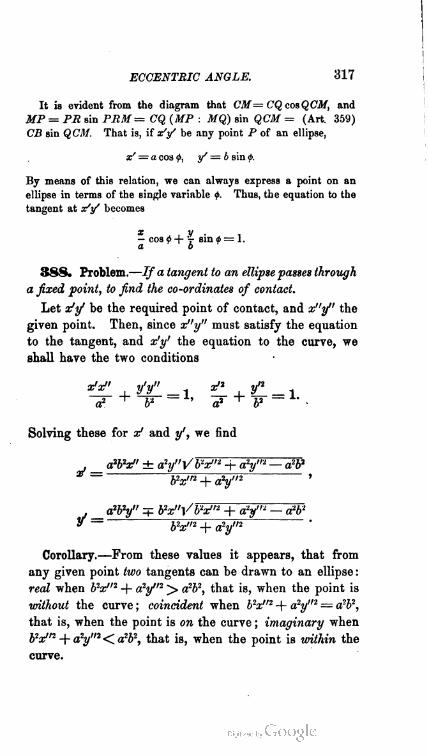
ECCENTRIC ANGLE. 317
It is evident from the diagram that CM=CQeosQCM, and
MP = PR sin PRM= CQ (MP : MQ) sin QCM = (Art. 359)
CB sin QCM. That is, if ar'y' be any point P of an ellipse,
3/' = a cos 0, y' = b sin 0.
By means of this relation, we can always express a point on an
ellipse in terms of the single variable ^. Thus, the equation to the
tangent at x'y' becomes
x , v . ,— cos if> + r sin 6 = 1.a o
3SS. Problem.—If a tangent to an ellipse passes through
a fixed point, to find the co-ordinates of contact.
Let x'y1 be the required point of contact, and x"y" the
given point. Then, since x"y" must satisfy the equation
to the tangent, and x'y' the equation to the curve, we
shall have the two conditions
a2 + b1 ~ ' a? i" b2 ~
Solving these for x' and y\ we find
, aW ± a2y"Vblx"1 + ay"— a2b2
, a2b2y" q= Px'Vtfx"2 + ay" — a262
Corollary.—From these values it appears, that from
any given point two tangents can be drawn to an ellipse :
real when b2x"2 + a2y"2 > a2b2, that is, when the point is
without the curve ; coincident when 62x"2 + a2?/"2 = «2&2,
that is, when the point is on the curve ; imaginary when
bV2 + a2y"2< a262, that is, when the point is within the
curve.
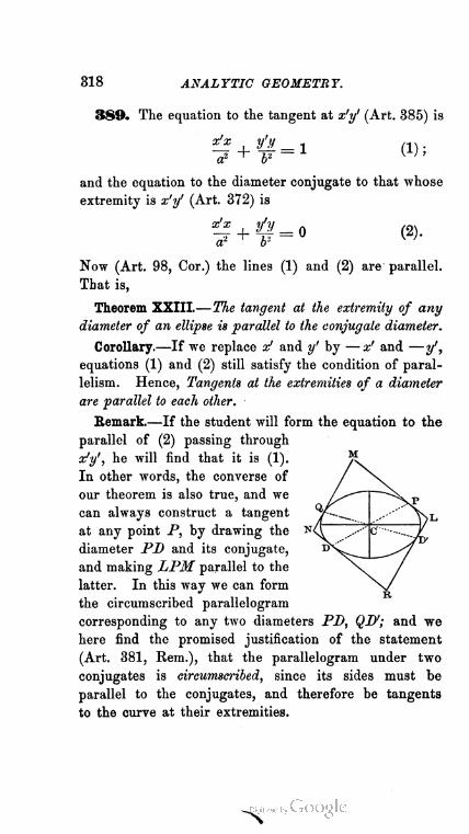
318 ANALYTIC GEOMETRY.
The equation to the tangent at x'y' (Art. 385) is
(i);
a2 + b1
and the equation to the diameter conjugate to that whose
extremity is x'y' (Art. 372) is
x[x -ijy
a* ^ V= 0 (2).
Now (Art. 98, Cor.) the lines (1) and (2) are parallel.
That is,
Theorem XXIII.—The tangent at the extremity of any
diameter of an ellipse is parallel to the conjugate diameter.
Corollary.—If we replace x' and y' by — x' and —y1,
equations (1) and (2) still satisfy the condition of paral
lelism. Hence, Tangents at the extremities of a diameter
are parallel to each other.
Remark,—If the student will form the equation to the
parallel of (2) passing through
x'y', he will find that it is (1).
In other words, the converse of
our theorem is also true, and we
can always construct a tangent
at any point P, by drawing the
diameter PD and its conjugate,
and making LPM parallel to the
latter. In this way we can form
the circumscribed parallelogram
corresponding to any two diameters PD, QD1; and we
here find the promised justification of the statement
(Art. 381, Rem.), that the parallelogram under two
conjugates is circumscribed, since its sides must be
parallel to the conjugates, and therefore be tangents
to the curve at their extremities.
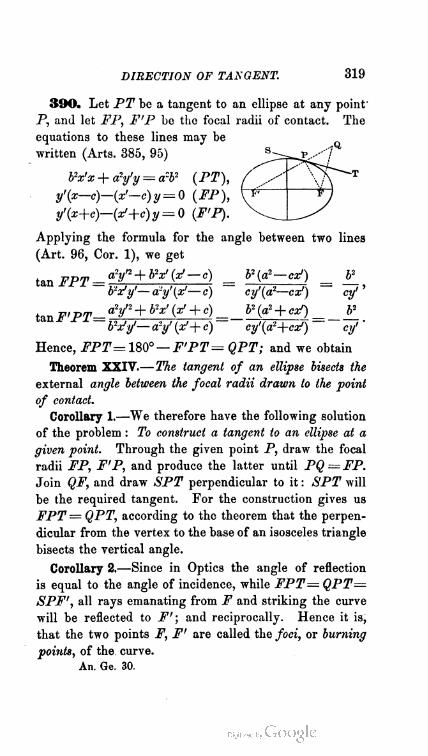
DIRECTION OF TANGENT. 319
390. Let PT be a tangent to an ellipse at any point'
P, and let FP, F'P be the focal radii of contact. The
equations to these lines may be
written (Arts. 385, 95)
b2x'x + a2y'y = a:b2 (PT),
y'(x—c)—(x'—c)y = 0 (FP),
y'(x+c)-(x'+c)y = 0 (F'P).
Applying the formula for the angle between two lines
(Art. 96, Cor. 1), we get
tanjppy^ay2+6y(*'-c) = b2(a2-cx>) = V_
b-x'y'— d-y'(x'— c) cy'(dl—cx') cy'''
tanF'PT= aY'+^'(x' + c) =_ b2(a2 + cx') = _ ¥_ _
b2xly>— dry' (x'-\- c) cy'(dl-\-cx') cy' '
Hence, FPT=180°— F'PT= QPT; and we obtain
Theorem XXIV.—The tangent of an ellipse bisects the
external angle between the focal radii drawn to the point
of contact.
Corollary 1.—We therefore have the following solution
of the problem : To construct a tangent to an ellipse at a
given point. Through the given point P, draw the focal
radii FP, F'P, and produce the latter until PQ=FP.
Join QF, and draw SPT perpendicular to it : SPT will
be the required tangent. For the construction gives us
FPT= QPT, according to the theorem that the perpen
dicular from the vertex to the base of an isosceles triangle
bisects the vertical angle.
Corollary 2.—Since in Optics the angle of reflection
is equal to the angle of incidence, while FPT= QPT=
SPF', all rays emanating from F and striking the curve
will be reflected to F'; and reciprocally. Hence it is,
that the two points F, F' are called the foci, or burning
points, of the curve.
An. Ge. 30.
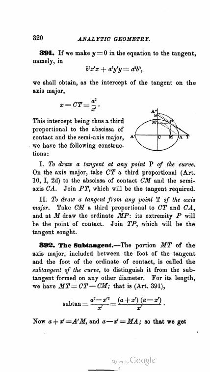
320 ANALYTIC GEOMETRY.
391. If we make y = 0 in the equation to the tangent,
namely, in
b-xfx + ary'y = a2b"-,
we shall obtain, as the intercept of the tangent on the
axis major,
x = CT=-,.
This intercept being thus a third
proportional to the abscissa of
contact and the semi-axis major,
we have the following construc
tions :
I. To draw a tangent at any point P of the curve.
On the axis major, take CT a third proportional (Art.
10, I, 2d) to the abscissa of contact CM and the semi-
axis CA. Join PT, which will be the tangent required.
II. To draw a tangent from any point T of the axis
major. Take CM a third proportional to CT and CA,
and at M draw the ordinate MP: its extremity P will
be the point of contact. Join TP, which will be the
tangent sought.
392. The Subtangent.—-The portion MT of the
axis major, included between the foot of the tangent
and the foot of the ordinate of contact, is called the
subtangent of the curve, to distinguish it from the sub-
tangent formed on any other diameter. For its length,
we have MT= CT—CM; that is (Art. 391),
subtan=^^^±4^).
x' ar
Now a + xZ—A'M, and a— x1=MA ; so that we get
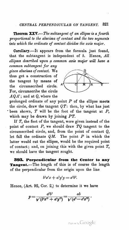
CENTRAL PERPENDICULAR ON TANGENT. 321
Theorem XXV.—The subtangent of an ellipse is a fourth
proportional to the abscissa of contact and the two segments
into which the ordinate of contact divides the axis major.
Corollary.—It appears from the formula just found,
that the subtangent is independent of b. Hence, All
ellipses described upon a common axis major will have a
common subtangent for any
given abscissa of contact. We
thus get a construction of
the tangent by means of
the circumscribed circle.
For, circumscribe the circle
A QA' ; and at Q, where the
prolonged ordinate of any point P of the ellipse meets
the circle, draw the tangent QT: then, by what has just
* been shown, T will be the foot of the tangent at P,
which may be drawn by joining PT.
If T, the foot of the tangent, were given instead of the
point of contact P, we should draw TQ tangent to the
circumscribed circle, and, from the point of contact Q,
let fall the ordinate QM. The point P in which the
latter would cut the ellipse, would be the required point
of contact ; and, on joining this with the given point T,
we should have the tangent sought.
393. Perpendicular from the Center to any
Tangent.—The length of this is of course the length
of the perpendicular from the origin upon the line
b2x'x + dry'y — a7b2.
Hence, (Art. 92, Cor. 2,) to determine it we have
_ a?V ab
P~y/{^xn + aiy'2)~^/{a2—e2xn) '

322 ANALYTIC GEOMETRY.
But (Art. 376) a2 — eV2 = b'2. Hence, finally,
Expressing this relation in ordinary language, and ob
serving the principle of Art. 389, we obtain
Theorem XXVI.—The central perpendicular upon any
tangent of an ellipse is a fourth proportional to the parallel
semi-diameter and the semi-axes.
394. Central Perpendicular In terms of Its Inclination
to tlie Axis Major.—For the length of the perpendicular from the
origin upon the tangent whose equation (Art. 386, Cor.) is
y = mx + V'mW + 62,
we have (Art. 92, Cor. 2)
Now let 0 = the inclination of the perpendicular: then will
m = — cot 0, and we get
p = vVcos20 + 6'-sin20.
393* The following investigation will illustrate the usefulness
of the expression last obtained, and of the equation to the tangent
from which it is derived.
Let it be required to find the locus of the intersection of tangents
to an ellipse which cut at right angles. The inclinations of the two
tangents will be 0 and 90° + 0; and we shall have, for their central
perpendiculars,
p2 = a2cos20 + 62sin20, pn = a2sin20 + 4W0.
. •. y+y= a' + 6».
Now, if xy be the intersection of the tangents, the square of its dis
tance from the center will be x1 -f- y2 =p2 + p/i. Hence, from what
has just been proved, the co-ordinates of intersection are connected
by the constant relation
*, + y,= aJ + i*:

FOCAL PERPENDICULARS ON TANGENT. 323
which is the equation to a circle concentric with the ellipse, and
circumscribed about the rectangle of the axes.* That is,
Theorem XXVII.—The locus of the intersection of tangents which
cut each other at right angles, is the circle circumscribed about the
rectangle formed on the axes.
396. Perpendiculars from the Foci to any
Tangent.—The co-ordinates of the right-hand focus
are x = ae, y — 0 : hence, for the length of the perpen
dicular from F upon the tangent JV.-c + cPy'y — a2b2, we
have (Art. 105, Cor. 2)
b2x'ae — a2b2 ab2(ex'— a) b (ex'— a)
P ~ x/{b4xr2 + a4y'2) ~ ab ^(a2 — e2x'2) = i/(a2— e2x'2) '
Now (Art. 360) a — ex' — p, the right-hand focal radius
of contact ; and (Art. 376) a2 — e2x'2 = b'2, the square of
the semi-diameter conjugate to the point of contact.
Hence, for the right-hand focus,
bp
P = t-
Similarly, for the left-hand focus, we should find
, bp'
?=-¥'
Corollary.—By Art. 377, b'2 =pp' : hence, after squar
ing the expressions just obtained,
2 b2p n b2p'
P P
formulae which, in certain cases, are more useful than
the preceding.
s This locus may be obtained even more readily, as follows : — The
equations to the two tangents (Arts. 386, Cor. ; 99, Cor.) may be written
y — mx = ^m2a2 + 62, my + x= Vm'b'1 + a2.
Squaring and adding these expressions, we eliminate m, and get

324 ANALYTIC GEOMETRY.
397. Comparing the two results of Art. 396, we get
p : p' : : p : p',
a relation expressed in ordinary terms by
Theorem XXVIII.—The focal perpendiculars upon any
tangent of an ellipse are proportional to the adjacent focal
radii of contact.
398. Multiplying together the values of p and p',
and observing Art. 377, we obtain
PP' = t>\
which is the algebraic expression of
Theorem XXIX.—The rectangle under the focal perpen
diculars upon any tangent is constant, and equal to the
square on the semi-axis minor.
399. The equation to any tangent of an ellipse
(Art. 386, Cor.) being
y — mx = Vni'd2 + b2,
that of the focal perpendicular, which passes through
(vV— b\ 0), may be written (Art. 103, Cor. 2)
my + x = Va2— b2.
Squaring these equations, and adding them together,
we obtain
x2 + y2 = a2
as the equation to the locus of the point in which the focal
perpendicular meets the tangent. Hence, (Art. 136,)
Theorem XXX.—The locus of the foot of the focal per
pendicular upon any tangent of an ellipse, is the circle
circumscribed about the curve.
Corollary.—From this property, we obtain the follow
ing method of constructing a tangent to any ellipse, —

GENERIC CONSTR UCTION FOR TANGENT. 325
a method which deserves special attention, because it is
applicable alike to all the Conies, and holds good whether
the point through which the tangent is drawn be without
the curve or upon it.
To draw a tangent to an ellipse through any given
point.—Join the given point P with either focus F, and
upon PF as a diameter describe
a semicircle. Then through Q,
where this semicircle cuts the
circumscribed circle, draw PQ:
it will touch the ellipse at some
point T. For the angle FQP is
inscribed in a semicircle, and Q is therefore the foot of
the focal perpendicular upon PQ.
In case, as in the second dia
gram annexed, the point P is on
the ellipse, the circle described
on PF will be found to touch
the circumscribed circle at Q
(see Ex. 8, p. 359). The con
struction still holds, however ; for the point of contact Q
must lie on the line joining the centers of the auxiliary
and circumscribed circles, and may therefore be found
at once by joining C with the middle point of PF, and
producing the line thus formed until it meets the cir
cumscribed circle.
Remark.—It is obvious that the ordinary method of drawing a
tangent to a circle through a given point (Geom., 230), is only a
particular case of the method here described : the case, namely,
where the two foci of the ellipse become coincident at C, when of
course the ellipse becomes identical with the circumscribed circle.
We have seen (Art. 388, Cor.) that two tangents can, in general,
be drawn to an ellipse from a given point P; and the construction
evidently corroborates this, since the auxiliary circle PQF must in
general cut the circumscribed circle in two points.
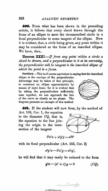
326 ANALYTIC GEOMETRY.
400. From what has been shown in the preceding
article, it follows that every chord drawn through the
focus of an ellipse to meet the circumscribed circle is a
focal perpendicular to some tangent of the ellipse. Now
it is evident, that, a circle being given, any point within it
may be considered as the focus of an inscribed ellipse.
We have, then,
Theorem XXXI.—If from any point within a circle a
chord be drawn, and a perpendicular to it at its extremity,
the perpendicular will be tangent to the inscribed ellipse of
which the point is a focus.
Corollary—This is of course equivalent to saying that the inscribed
ellipse is the envelope of the perpendicular.
Advantage may be taken of this principle,
to construct an ellipse approximately by
means of right lines; for it is evident that
by taking the perpendiculars sufficiently
near together, we can approach the line
of the curve as closely as we please. The
diagram presents an example of this method.
401. If the student will now form, by the method of
Art. 108, Cor. 1, the equation
to the diameter CQ, that is,
the equation to the line join
ing the origin to the inter
section of the tangent
b2x'x -+- a2y'y = a2b2
with its focal perpendicular (Art. 103, Cor. 2)
a2y'x— b2x'y — a2cy',
he will find that it may easily be reduced to the form
y'x-(x' + c)y = 0 (CQ).
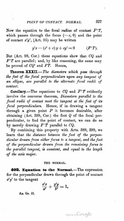
POINT OF CONTACT. NORMAL. 327
Now the equation to the focal radius of contaet F'T,
which passes through the focus (— c, 0) and the point
of contact x'y', (Art. 95) may be written
y'x— (x'+c)y + cy' = 0 (F'T).
But (Art. 98, Cor.) these equations show that CQ and
F'T are parallel ; and, by like reasoning, the same may
be proved of CQ' and FT. Hence,
Theorem XXXII.—The diameters which pass through
the feet of the focal perpendiculars upon any tangent of
an ellipse, are parallel to the alternate focal radii of
contact.
Corollary.—The equations to CQ and F'T evidently
involve the converse theorem, Diameters parallel to the
focal radii of contact meet the tangent at the feet of its
focal perpendiculars. Hence, if in drawing a tangent
through a given point P it becomes desirable, after
obtaining (Art. 399, Cor.) the foot Q of the focal per
pendicular, to find the point of contact, we can do so
by merely drawing F'T parallel to CQ.
By combining this property with Arts. 389, 399, we
learn that the distance between the foot of the perpen
dicular drawn from either focus to a tangent, and the foot
of the perpendicular drawn from the remaining focus to
the parallel tangent, is constant, and equal to the length
of the axis major.
THE NORMAL.
402. Equation to the Normal.—The expression
for the perpendicular drawn through the point of contact
x'y' to the tangent
x'x ,y'y_A
a? + b2 - '
An. Ge. 31.
328 ANALYTIC GEOMETRY.
according to Art. 103, Cor. 2, is
f5(*-*o= ^-y)-
Clearing of fractions, dividing through by x'-yf, and
putting (Art. 151) c2 for a2 — 62, we may write the
equation sought
a2x b2y _ ,
403. If we seek the angle <p made by the normal
with the left-hand focal radius of contact F'T, whose
equation is y'x— (x' + c) y + ey' — 0, we get (Art. 96,
Cor. 1)
a/ ey1
taDy~62(^+c) |~~~lr"
Similarly, for the angle <p' made with the normal by the
right-hand focal radius of contact FT, wo get
a2(s' — e) _ b,
an f — ^ 62 (a/ — c) ~ Vs '
xf + y>
Hence <p' = <p ; or, the normal makes equal angles with
the two focal radii drawn to the point of contact, and
vre have
Theorem XXXIII.—The normal of an ellipse bisects the
internal angle between the focal radii of contact.
Corollary 1.—This property enables us to construct a
normal at a given point on the curve. For let P be the
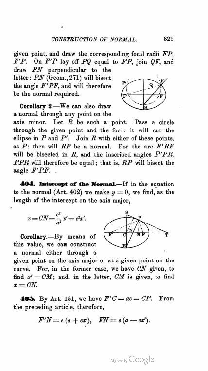
CONSTRUCTION OF NORMAL. 329
given point, and draw the corresponding focal radii FP,
F'P. On F'P lay off PQ equal to FP, join QF, and
draw PN perpendicular to the
latter: PN (Geom., 271) will bisect
the angle F'PF, and will therefore
be the normal required.
Corollary 2.—We can also draw
a normal through any point on the
axis minor. Let R be such a point. Pass a circle
through the given point and the foci : it will cut the
ellipse in P and P'. Join R with either of these points,
as P: then will RP be a normal. For the arc F'RF
will be bisected in R, and the inscribed angles F'PR,
FPR will therefore be equal ; that is, RP will bisect the
angle F'PF.
404. Intercept of the Normal.—If in the equation
to the normal (Art. 402) we make y = 0, we find, as the
length of the intercept on the axis major,
x =CN=-x'=e2x'.
a2
Corollary.—By means of
this value, we can construct
a normal either through a
given point on the axis major or at a given point on the
curve. For, in the former case, we have ON given, to
find x' = CM; and, in the latter, CM is given, to find
x=ON.
405. By Art. 151, we have F'C=ae = GF. From
the preceding article, therefore,
F'N= e (a + eaf), FN=e(a— ex1).

330 ANALYTIC GEOMETRY.
Hence (Art. 360), F'N : FN=F'P : FP; that is,
Theorem XXXIV.— The normal of an ellipse cuts the
distance between the foci in segments proportional to the
adjacent focal radii of contact.
406. ^Length of the Subnormal.—The portion
NM of the axis major, in
cluded between the foot of
the normal and that of the
ordinate of contact, is called
the subnormal of the curve,
to distinguish it from that
formed on any other diameter. For its length, we have
NM=QM—GN=a/-eV= (1— That is (Art. 151),
subnor = ^ x'.
a'
407. Comparing the results of Arts. 404 and 406,
ON : NM= c2 : V. Hence, as c2 = a2 — b2, we get
Theorem XXXV.—The normal of an ellipse cuts the
abscissa of contact in the constant ratio (a2 — b2) : b2.
408. ^Length of the Normal.—By this is meant
the portion of the normal intercepted between the point
of contact and either axis. We have, then,
PN2=PM2 +NW=y'2 4- *»= bl (a2 — eV2).
a4 or
Hence, since (Art. 376) a2 — eV2 = b'2,
PN=™.a
By similar reasoning, the details of which are left for
the student to supply,

SEGMENTS OF NORMAL. 331
409. From the foregoing, it follows immediately that
PN.PR—b'2. In other words, we have obtained
Theorem XXXVI.—The rectangle under the segments
formed by the two axes upon the normal is equal to the
square on the semi-diameter conjugate to the point of
contact.
Corollary.—We have proved (Art. 377) that b'2 — pp'.
Hence, PN.PR—pp'; and we get the additional property :
The rectangle under the segments of the normal is equal to
the rectangle under the focal radii of contact.
41©. It has been shown (Art. 393) that, for the length
of the central perpendicular upon any tangent, we have
CQ = fr
Therefore, CQ.PR = a2, and CQ.PN=b2. That is,
Theorem XXXVII.—The rectangle under the normal
and the central perpendicular upon the corresponding
tangent is constant, and equal to the square on the
semi-axis other than the one to which the normal is
measured.
SUPPLEMENTAL AND FOCAL CHOKDS.
411. Definition.—By Supplemental Chords of an
ellipse, are meant two chords passing b
through the opposite extremities of
any diameter, and intersecting on A,/S^__
the curve. \J
Thus, BP, B'P are supplemental ly^v^^
with respect to the diameter B'B;
and AQ, A'Q, with respect to the axis major.

332 ANALYTIC GEOMETRY.
412. Condition that Chords of an Ellipse be
Supplemental.—Let <p be the inclination of any chord
DP, and <p' that of the supplemental chord D"P. Then,
since (Art. 149) every diameter is bisected by the center C,
if the co-ordinates of D be x', y', those of D' will be — x',
— y'; and the equations to DP, D'P (Art. 101, Cor. 1)
may be written
y — y'^'x— x1) tan tp, y + y' = (x + x') tan <p'.
Hence, at the intersection P, we shall have the condition
y2 — y'2= (x2 — x12) tan tp tan <p',
in which xy, x'y' , being both upon the curve, are so con
nected (Art. 147) that
x2 — x'- a2
The supplemental chords are therefore subject to the
constant condition
b2tan w tan w = = .
7 a1
413. If d and Q' are the respective inclinations of two
diameters drawn parallel to a pair of supplemental chords,
then d = <p and 6'=<p'; and, from the preceding condition,
we have
b2tan d tan 6' — ■ .
a2
But this (Art. 370) is the condition that the diameters
corresponding to 0 and 0' shall be conjugate. Hence,
Theorem XXXVIII.—Diameters of an ellipse which are
parallel to supplemental chords are conjugate.

SUPPLEMENTAL CHORDS. 333
Remark.—This theorem may be otherwise stated:
If a diameter be parallel to one of two supplemental
chords, its conjugate will be parallel to the other. It
therefore gives rise to the following constructions.
Corollary 1.—To construct a pair of conjugate diameters
at a given inclination. On any diameter, describe (Geom.,
231) an arc containing the given angle, and join either
of the remaining points in which the circle cuts the ellipse
with the extremities of the diameter : the diameters drawn
parallel to the supplemental chords thus formed will be
the conjugates required.
Caution.—It should be borne in mind, in connection with this
problem, that the inclination of two conjugates in an ellipse is
subject to a restriction, and is not any angle we please, but only
(Arts. 381, Cor. 1 ; 382, Cor. 2) any angle between the limits 90° and
sin-^ab : (aJ + b').
Corollary 2.—To construct a tangent parallel to a given
right line. Let LM represent the given line. The point
of contact of the required tan
gent (Art. 389) is the extrem
ity of the diameter conjugate
to that drawn parallel to LM.
Draw, then, the chordA Q par
allel to LM from the extremity
of the axis major, and the di
ameter DP parallel to the supplemental chord QA' :
the line PT drawn through the extremity P of this
diameter, parallel to the given line LM, will be the
tangent sought.
Corollary 3.—To construct the axes in the empty curve.
Draw any two parallel chords, bisect them, and form the
corresponding diameter, say BP. On the latter, describe
a semicircle cutting the ellipse in R. Join DR, RP:
334 ANALYTIC GEOMETRY.
they will be supplemental chords of the circle, and there
fore (Art. 317, Cor.) at right angles. They will also be
supplemental chords of the ellipse : hence A'A, B'B,
drawn parallel to them through C, will be the rectangular
conjugates of the curve ; that is, its axes.
414. Definition.—A Focal Chord of an ellipse, and in
fact of any conic, is simply a chord drawn through a focus.
The focal chords possess some special properties,
several of which, in the form corresponding to the
Ellipse, will be given in the examples at the close of
this Chapter. One of them, however, has an important
bearing upon the properties of a certain element of the
curve, and we shall therefore develop it here.
413. The equation to any focal chord, having the
inclination 0 to the axis major, may be written (Art.
101, Cor. 3)
y x — ae ^
sinO cos 0 '
I being the distance from the focus to any point on the
chord. At the intersections of the chord with the curve,
we shall therefore have (Art. 147)
(a2 sin2 6 + b2 cos2 6) P + W ae cos 0. 1 = b\
The roots of this quadratic are readily found to be
b2 (1 -f e cos 0) ri b2 (1 — e cos d)
a (1 — e2cos2#) ' a (1 — e2cos20)
But these roots are the values of the two opposite seg
ments into which the focus divides the chord. Neglecting,
then, the sign of I", we have, for the length of the whole
chord,
,2 b2cno = - . = .
a 1 — <r cos2 0

ELLIPSE REFERRED TO CONJUGATES. 335
Now (Art. 365) the second factor in this expression is
the square on the semi-diameter whose inclination is 0.
Hence, if we put a' = the semi-diameter parallel to the
chord, we get
2a'2 (2a')2cho = = v n ' :
a la
a property which we may express by
Theorem XXXIX.—Any focal chord of an ellipse is a
third proportional to the axis major and the diameter
parallel to the chord.
Remark.—This result is exemplified in the value found
(Art. 357, Cor.) for the latus rectum, which is the focal
chord parallel to the axis minor.
ii. The Curve referred to any two Conjugates.
DIAMETRAL PROPERTIES.
416. We are now ready to consider the Ellipse from
a point of view somewhat higher than the one we have
hitherto occupied, and shall presently discover that many
of the properties we have developed are only particular
cases of theorems more generic. Heretofore, we have
referred the curve to its axes : let us now refer it to any
two conjugate diameters.
417. Equation to the Ellipse, referred to any
two Conjugate Diameters.—To obtain this, we must
transform the equation of Art. 147,

336 ANALYTIC GEOMETRY.
from rectangular axes to oblique ones having the respective
inclinations 0 and 0' to the axis major. Replacing (Art.
56, Cor. 1) a; and y by x cos 0 + y cos 0' and z sin 0 + ?/ sin 0',
we obtain, after obvious reductions,
(a2 sin2 0 + ¥ cos2 (?) x2 + (a2 sin2 d'+ b2 cos2 0') #2
+ 2 (a2 sin 0 sin 0' + b2 cos 0 cos 0') xy=aW.
But, as the new reference-axes are conjugate diameters,
we have, by a single transformation of the condition in
Art. 370,
a2 sin 0 sin 0' + b2 cos 0 cos 0' = 0.
The transformed equation is therefore in fact
(a2 sin2 0 + b2 cos2 0) x2 + (a2 sin2 0' + b2 cos2 0') «/2 = a2b2.
In this, the co-efficients are still functions of the semi-
axes ; but if we seek the values of the semi-conjugates
a' and b' by finding (Art. 73) the intercepts of the curve
upon the new axes of reference, we readily obtain
a2sin20 + 62cos20 = ^ , «2sin20' + 62cos20' = ^ .a'1 bn
Hence, the required equation, in its final form, is
- + -^=1.
418. Comparing this equation with that of Art. 147,
and remembering (Art. 372, Cor.) that the axes are a
case of conjugates, it becomes evident that the equation
hitherto used, namely,
t J_ £ — 1ai 1- j2 — h
DIAMETRAL PROPERTIES. 337
is only the particular form assumed by the general one
we have now obtained, when the reference-conjugates
have the specific lengths 2a, 2b, and are at right angles
to each other. Moreover, from the identity of form in
the two equations, we see at once that the transforma
tions applied to
t _i_ t — 1
a2 b2
are equally applicable to
a'2 ^ b'2 ~ '
and that the theorems derived from the former may
therefore be immediately extended to any conjugate
diameters, provided they do not involve the inclination
of the reference-axes. Thus, we learn that the theorems
of Arts. 357, 358 are particular cases of the following :
Theorem XL.—The squares on the ordinates to any
diameter of an ellipse are proportional to the rectangles
under the corresponding segments of the diameter.
Theorem XLI.—The square on any diameter of an
ellipse is to the square on its conjugate, as the rectangle
tinder any two segments of the diameter is to the square
on the corresponding ordinate. -v,
419. The equation of Art. 417 may of course be
written
b'2
The equation to a circle described upon the diameter
2a' is
y2 — a'2— 7?.

338 ANALYTIC GEOMETRY.
Supposing, then, that we consider those ordinates of the
two curves that correspond to a common abscissa, we
get
ye-yc = b': a',
and therefore have the following extension of the rela
tion (Art. 359) between the Ellipse and the circumscribed
circle :
Theorem XLII.—The ordinate to any diameter of an
ellipse is to the corresponding ordinate of the circle de
scribed on that diameter, as the conjugate of the diameter
is to the diameter itself.
Corollary 1.—Hence, given two _ci .
conjugate diameters in position and /^f^^fv^o.
magnitude, we may construct the /y \ /
curve by points, as follows : — On (! i j ])
each of the given diameters DL, ^n^,
D'L', describe a circle. At M, '<::z^/
any point on the diameter selected
for the axis of x, set up a rectangular ordinate of the
corresponding circle, meeting the curve in Q, and draw
MP parallel to the conjugate diameter D'L'. Join Q,
the extremity of the circular ordinate, to the center C,
and through 0, where QC cuts the inner circle, draw OR
parallel to DL : then will RM measure the distance of 0
from DL. From M as a center, with the radius MR,
describe an arc cutting MP in P: then will P be a
point of the required ellipse. For MP — MR = the
perpendicular from 0 upon CD. Hence, MP : MQ =
CO:CQ = V : a'.
Corollary 2.—The use of the equation x2 + y2 = a'2 in
the preceding investigation, to denote a circle described
upon a diameter of an ellipse, suggests a point of con
siderable importance. The equation denotes such a
ELLIPSE REFERRED TO EQ UI-CONJUGATES. 339
circle, only on the supposition that the axes of refer
ence are rectangular; and, in the construction just
explained, the ordinate MQ was drawn in accordance
with this principle.
The equation, however, is susceptible of a more gen
eral interpretation. It evidently arises from the general
equation
fL 4- t- — 1an "I" bn — ^
whenever a' = b'. In other words, the equation
+ y2 — a'2i
when the reference-axes are oblique, denotes an ellipse
referred to its equi-conjugate diameters.
420. By throwing the equation of Art. 417 into the
form
b'2
and subjecting it to an analysis precisely like that of
Art. 361, we can determine the figure of the Ellipse
with respect to any two conjugates. It will thus appear
that the curve is oblong, closed, continuous in extent,
and symmetric not only to the axis major and axis minor,
but to any diameter whatever.
CONJUGATE PROPERTIES OF THE TANGENT.
421. Equation to the Tangent, referred to any
two Conjugate Diameters.—From the relation estab
lished (Art. 418) between the equations
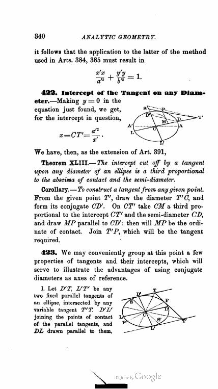
340 ANALYTIC GEOMETRY.
it follows that the application to the latter of the method
used in Arts. 384, 385 must result in
x"xy'y
a'2 + bn ~~ *'
433. Intercept or the Tangent on any Diam
eter.—Making y = 0 in the
equation just found, we get,
for the intercept in question,
a'2x=CT'=~.
x'
We have, then, as the extension of Art. 391,
Theorem XLIII.—The intercept cut off by a tangent
upon any diameter of an ellipse is a third proportional
to the abscissa of contact and the semi-diameter.
Corollary.—To construct a tangent from anygiven point.
From the given point T', draw the diameter T'C, and
form its conjugate CD'. On OT' take CM a third pro
portional to the intercept CT' and the semi-diameter CD,
and draw MP parallel to CD1 : then will MP be the ordi
nate of contact. Join T'P, which will be the tangent
required.
433. We may conveniently group at this point a few
properties of tangents and their intercepts, which will
serve to illustrate the advantages of using conjugate
diameters as axes of reference.
I. Let VT, L'T' be any
two fixed parallel tangents of
an ellipse, intersected by any
variable tangent T'T. I/L'
joining the points of contact
of the parallel tangents, and
DL drawn parallel to them,
X

TANGENT REFERRED TO CONJUGATES. 341
(Art. 389) will be conjngate diameters. Taking these for reference-
axes, the equation to the variable tangent T'T is
f^f 4. — l
a'1 ^ b"
In this, making y successively equal to + b' and — V, we obtain
Hence, multiplying together the two values of x, and substituting
for i/72 its value from the equation to the Ellipse, we get
JYT. L'T' = a".
Interpreting this relation in ordinary language, we have
Theorem XLIV.—The rectangle under the intercepts cut off upon
two fixed parallel tangents by any variable tangent of an ellipse is
constant, and equal to the square on the semi-diameter parallel to the
two tangents.
II. If we take for axes of reference the diameter CP drawn to
the point of contact of any variable tangent, and the conjugate
diameter SS', the equations to any two fixed parallel tangents
IZT, L'T' will be
x'x I v'y _ i ofx tfy _
a'1 ~t~ bn ' of' ~l~ bn
Making a; = a/ in each of these, and remembering (Art. 389) that
the axis of y (SS') is parallel to the variable tangent T'T, we get
Hence, after substituting for y'2 from the equation to the curve,
PT. PT'= b'2,
the sign of the second factor being disregarded, as we are only
concerned with the area of the rectangle. We have, then,
Theorem XLV—The rectangle under the intercepts cut off upon
any variable tangent of an ellipse by two fixed parallel tangents is
variable, being equal to the square on the semi-diameter parallel to the
tangent.
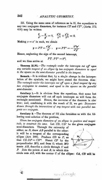
342 ANALYTIC GEOMETRY.
III. Using the same axes of reference as in II, the equations to
any two conjugate diameters, for instance C^and CT', (Arts. 372,
418) may be written '
9 _y — n — n
x1 y> ~ a" b'1 ~
Making x = a' in each, we obtain
Hence, neglecting the sign of the second intercept,
FT. PT' = bn,
and we thus arrive at
Theorem XLVI.— The rectangle tinder the intercepts cut off upon
any variable tangent of an ellipse by two conjugate diameters is equal
to the square on the semi-diameter parallel to the tangent.
Remark.—It is evident that, by a single change in the interpre
tation of the symbols, we might have stated the theorem thus:
The rectangle under the intercepts cut off upon a fixed tangent by any
two conjugates is constant, and equal to the square on the parallel
semi-diameter.
Corollary 1.—It is obvious from the equations, that none but
conjugate diameters will cut off such intercepts as will form the
rectangle mentioned. Hence, the converse of the theorem is also
true; and, combining it with the result of II, we get: Diameters
drawn through the intersections of any tangent with two parallel tan
gents arc conjugate.
Corollary 2.—The theorem of 111 also furnishes us with the fol
lowing neat solution of the problem,
Given two conjugate diameters of an ellipse in position and magni
tude, to construct the axes. Let CD, CD' be the given conjugate
semi-diameters. Through the extremity of
either, as D, draw AD parallel to the other: '
it will be a tangent of the corresponding
ellipse (Art. 389). Produce CD to P, so \
that CD.DP= CD"1. Bisect CP by the B^"7&~t)":;;"^A
perpendicular MO, and from O, where MO ^/--~'~~ j.
meets AB, describe a circle through C and V„
P. Join the points A and B, in which this
circle cuts AB, with the center C of the ellipse : CA, CB will be

SUBTANGENT IN GENERAL. 343
the axes sought. For (Geom., 331) AD.DB= CD DP= Ciy\ and
therefore (Th. xlvi) CA, CB are conjugate diameters. Moreover,
since ACB is inscribed in a semicircle, they are the rectangular
conjugates of the curve; or, in other words, the axes.
424. Subtangent to any Diameter.—This being
the portion of any diameter intercepted between the
foot T' of a tangent, and the foot M of the ordinate
of contact, we have, for its
length, MT> = CT' — CM. ,.;.v -H.
Hence, (Art. 422,)
a'2 xn
subtan' = ;
x'
That is, since a' + x1 = LM,
and a' — x' = MP, The subtangent to any diameter of an
ellipse is a fourth proportional to the abscissa of contact
and the corresponding segments of the diameter.
Corollary.—This value is independent of the length
of the conjugate semi-diameter b'; and, if we compare
it with that of the subtangent in the circle x2 + y2 = a'2
described upon the diameter which serves as the axis
of x, we find (Art. 311) that the two are equal. Hence
the following construction :
To draw a tangent to an ellipse from any given point.
Let T' be the given point. Through it draw the diameter
T'DL ; upon DL describe a circle, and form its tangent
TQ passing through the given point. Let fall QM per
pendicular to DL, and through its foot M draw PP' a
. double ordinate to the diameter DL : the points P, P'
in which this meets the curve will be the points of con
tact of the two possible tangents from T', either of which
may be obtained by joining T' to the proper point of
contact.
An. Ge. 32.
344 ANALYTIC GEOMETRY.
Remark.—It is obvious that the same principle may
be used to construct a tangent at any point P of the
curve, by simply drawing any diameter and its conjugate,
forming the corresponding ordinate of the ellipse from P,
and erecting at its foot the ordinate MQ of the circle
described on the diameter first drawn : the tangent to
this circle at Q will determine the foot T' of the required
tangent to the ellipse. This method is very convenient
when the curve only, or an arc of it, is given ; but, when
the axes are known, the construction described in the
corollary to Art. 392 is preferable.
425. If we multiply the value of the subtangent by
the abscissa of contact x1, we get x' subtan' = a'2 — x12.
Comparing this with the square on the ordinate of
contact, as given by the equation to the curve, namely,
y'2=b^(a'2 -*'*)>
we obtain x' subtan' : y12 — a'2 : b'2, a relation expressed
by
Theorem XLVII.—The rectangle under the subtangent
and the abscissa of contact is to the square on the ordinate
of contact, as the square on the corresponding diameter is
to the square on its conjugate.
426. The equations to the tangents at the extrem
ities of any chord of an ellipse, by taking for axes the
diameter parallel to the chord, and its conjugate, may
be written

PARAMETER OF THE ELLIPSE. 345
Eliminating between these, we find that the co-ordinates
of the point in which the tangents intersect are
a'2 n
Hence, comparing Arts. 369 ; 49, Cor. 1, we have
Theorem XLVIII.— Tangents at the extremities of any
chord of an ellipse meet on the diameter which bisects that
chord.
PARAMETERS.
4137* Definitions.—The Parameter of an ellipse,
with respect to any diameter, is a third proportional to
the diameter and its conjugate. Thus, if a', V denote
the lengths of any two conjugate semi-diameters, we
shall have, for the value of the corresponding parameter,
parameter(26')2 _ 2b'2
2a'
The parameter with respect to the axis major, is called
the principal parameter ; or, the parameter of the curve.
We shall represent its length by the symbol 4p.
428. From the definition above, we have, for the value
of the parameter of the Ellipse,
2b24» =
a
Hence, (Art. 357, Cor.,) the principal parameter is iden
tical with the line which we named the latus rectum;
that is, it is the double ordinate drawn through the
focus to the axis major.
346 ANALYTIC GEOMETRY.
429. In Art. 415, we proved that the focal chord
(or double ordinate) parallel to any diameter is a third
proportional to the axis major and the diameter. Now
(Art. 366) the axis major is greater than any other
diameter—greater, therefore, than the diameter conju
gate to that of which the focal chord is a parallel,
unless the chord is the latus rectum. Hence,
Theorem XLIX.—No parameter of an ellipse, except
the principal, is equal in value to the corresponding
focal double ordinate.
POLE AND POLAR.
430. We can now show that the reciprocal relation
of points and right lines which we established (Arts.
318— 321) in the case of the Circle, is a property of
the generic curve of which the Circle is only a particu
lar case. We shall develop the conception of the polar
line in the Ellipse by the same steps as in the former
investigation.
431. Chord of Contact in the Ellipse.—Let x'-tf
be the fixed point from which the two tangents that
determine the chord are drawn, and a?,y„ x^y2 their
respective points of contact. Their equations (Art.
421) will be
^4_M_ 1 A-VA — 1an -T b,2 — an "I" hn ~ A>
But x'y' being upon both tangents, we have

POLAR JiV THE ELLIPSE. 347
That is, the co-ordinates of both points of contact satisfy
the equation
*te , tL — 1
a'2 ^ bn ~ '
This is therefore the equation to the chord of contact.
432. Locus of the Intersection of Tangents to
the Ellipse.—Let x'y' be the fixed point through
which the chord of contact belonging to two inter
secting tangents is drawn, and xly1 the intersection of
the tangents. The equation to the chord (Art. 431)
will be
5£ -j- M. — 1an -T- 0n — >
and, as x'y' is on the chord, we shall have the condition
a'2 b" ~ '
irrespective of the direction of the chord. The co-ordi
nates of intersection for the two tangents drawn at its
extremities must therefore always satisfy the equation
£!? -4- tl— 1 •a'2 "•" &'2 "
which is for that reason the equation to the required
locus.
433. Tangent and Chord of Contact Included
In the wider conception of the Polar.—The equa
tions to the tangent, to the chord of contact, and to the
locus of the intersection of tangents drawn at the ex
tremities of chords that pass through a fixed point, are
thus seen to be identical in form. These three lines are
therefore only different expressions of a common formal
law ; and, inasmuch as the fixed point x'y', in the case

348 ANALYTIC GEOMETRY.
of the chord of contact, is restricted to being without
the curve ; and, in that of the tangent, to being on the
curve ; while, in the case of the locus in question, it is
not restricted at all : it follows that the tangent and
chord of contact are cases of the locus, due to bringing
the point x'y' upon the curve or outside of it. More
over, the relation between the locus which thus absorbs
the tangent and chord of contact, and the fixed point
x'y', is that of polar reciprocity. For, by precisely the
same argument as that used (Art. 321) in the case of
the Circle, we have the twofold theorem :
I. Iffrom a fixed point chords be drawn to any ellipse,
and tangents to the curve be formed at the extremities of each
chord, the intersections of the several pairs of tangents will
lie on one right line.
II. Iffrom different points lying on one right line pairs
of tangents be drawn to any ellipse, their several chords
of contact will meet in one point.
It thus appears that the Ellipse imparts to every point
in its plane the power of determining a right line ; and
reciprocally.
434. Equation to the Polar with respect to an
Ellipse.—From what has been shown in the preceding
articles, it is evident that this equation, referred to any
pair of conjugate diameters, is
x'x y'y
an + hn -
x'y' being the point to which the polar corresponds.
Consequently, the equation referred to the axes of the
curve will be
x'v , tl — 1
a2 I" b2 —
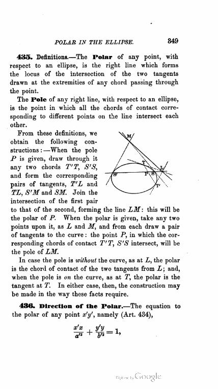
POLAR IN THE ELLIPSE. 349
435. Definitions.—The Polar of any point, with
respect to an ellipse, is the right line which forms
the locus of the intersection of the two tangents
drawn at the extremities of any chord passing through
the point.
The Pole of any right line, with respect to an ellipse,
is the point in which all the chords of contact corre
sponding to different points on the line intersect each
other.
From these definitions, we
obtain the following con
structions : —When the pole
P is given, draw through it
any two chords T'T, S'S,
and form the corresponding
pairs of tangents, T'L and
TL, S'M and SM. Join the
intersection of the first pair
to that of the second, forming the line LM: this will be
the polar of P. When the polar is given, take any two
points upon it, as L and M, and from each draw a pair
of tangents to the curve : the point P, in which the cor
responding chords of contact T'T, S'S intersect, will be
the pole of LM.
In case the pole is without the curve, as at L, the polar
is the chord of contact of the two tangents from L; and,
when the pole is on the curve, as at T, the polar is the
tangent at T. In either case, then, the construction may
be made in the way these facts require.
436. Direction of the Polar.—The equation to
the polar of any point x'y', namely (Art. 434),
i y'y _ iaii -f 5/2 — A>
350 ANALYTIC GEOMETRY.
when compared with that of the diameter conjugate to
the same point, namely (Arts. 372, 418),
^x . tfy _ nIP + bn - u'
shows (Art. 98, Cor.) that the polar and the diameter
are parallel. We have, then, the following extension
of the property reached in Art. 389 :
Theorem L.— The polar of any point, with respect to
an ellipse, is parallel to the diameter conjugate to that
which passes through the point.
437. Polars of Special Points.—It is easy to see,
by comparing the equations to the polar in the Ellipse
and in the Circle (Arts. 434, 323), that the general
properties of polars proved in Art. 324 are true in the
case of the Ellipse. We leave the student to convince
himself of this, and will here present certain special
properties of polars, which depend on taking the pole
at particular points.
If we substitute for x'y', in the equation of Art. 434,
the co-ordinates of the center, we shall get 1 = 0: an
expression conforming to the type (Art. 110)
C=0.
Hence, The polar of the center is a right line at infinity.
If in the same equation we make y'— 0, we shall get
Hence, The polar of any point on a diameter is a right
line parallel to the conjugate diameter, and its distance from
the center is a third proportional to the distance of the point
and the length of the semi-diameter.

POLAR OF THE FOCUS. 351
Similary, The polar of any point on the axis major is
the perpendicular whose distance from the center is a third
proportional to the distance of the point and the length
of the semi-axis.
Corollary.—The second of these properties obviously
leads to the following construction of the polar: —Join
the given point with the center of the curve, and, from
the latter as origin, lay oif upon the resulting diameter
a third proportional to the distance of the point and the
length of the semi-diameter. Through the point thus
reached, draw a parallel to the conjugate diameter,
which will be the polar required.
438. Polar of the Focus.—The equation to the
polar of either focus, by substituting (± ae, 0) for x'y'
in the second equation of Art. 434, is found to be
j_ ax= ± — .
e
Hence, The polar of either focus in an ellipse is the
perpendicular which cuts the axis major at a distance
from the center equal to a : e, measured on the same
side as the focus.
439. The distance of any point P of the curve from
either focal polar, say DM,
is evidently equal to the D
distance of that polar from
the center, diminished by the o
abscissa of the point. Thus,
PD^-x=a—^. R
e e
Now (Art. 360) a — ex = FP. Therefore,
FP _PD~e'
An. Ge. 33.
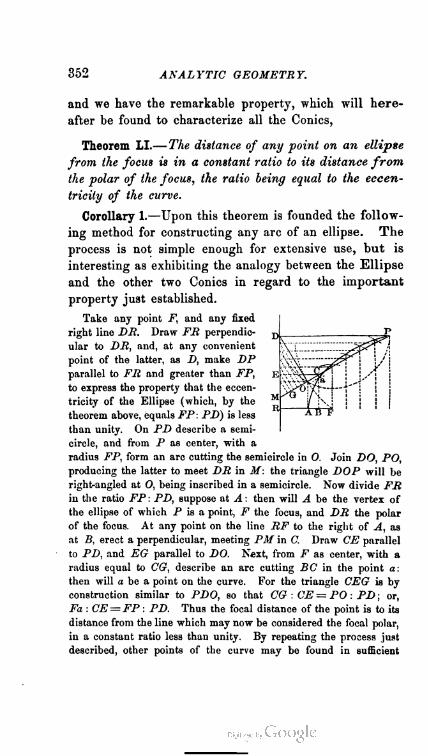
352 ANALYTIC GEOMETRY.
and we have the remarkable property, which will here
after be found to characterize all the Conies,
Theorem LI.—The distance of any point on an ellipse
from the focus is in a constant ratio to its distance from
the polar of the focus, the ratio being equal to the eccen
tricity of the curve.
Corollary 1.—Upon this theorem is founded the follow
ing method for constructing any arc of an ellipse. The
process is not simple enough for extensive use, but is
interesting as exhibiting the analogy between the Ellipse
and the other two Conies in regard to the important
property just established.
Take any point F, and any fixed
right line DR. Draw FR perpendic- D
ular to DR, and, at any convenient
point of the latter, as D, make DP
parallel to FR and greater than FP, js
to express the property that the eccen
tricity of the Ellipse (which, by the ^jj
theorem above, equals FP: PD) is less
than unity. On PD describe a semi
circle, and from P as center, with a
radius FP, form an are cutting the semicircle in O. Join DO, PO,
producing the latter to meet DR in M: the triangle DOP will be
right-angled at O, being inscribed in a semicircle. Now divide FR
in the ratio FP : PD, suppose at A : then will A be the vertex of
the ellipse of which P is a point, F the focus, and DR the polar
of the focus. At any point on the line RF to the right of A, as
at B, erect a perpendicular, meeting PM in C. Draw CE parallel
to PD, and EG parallel to DO. Next, from F as center, with a
radius equal to CG, describe an arc cutting BC in the point a:
then will a be a point on the curve. For the triangle CEG is by
construction similar to PDO, so that CG : CE— PO : PD ; or,
Fa : CE = FP : PD. Thus the foeal distance of the point is to its
distance from the line which may now be considered the focal polar,
in a constant ratio less than unity. By repeating the process just
described, other points of the curve may be found in sufficient

ELLIPSE DEFINED BY POLE AND POLAR. 353
numbers to determine its outline, and it can then be drawn
through them.
Corollary 2.—The fact has been brought to light
(Arts. 431—433), that the positions of the pole and
polar may be as near to or as remote from each other
as we please. It is therefore not only true that an
ellipse imparts to every point in its plane the power
of determining a right line, but any given right line
is the polar of any given point, with respect to some
ellipse. Now the construction just explained rests upon
this principle, and the given line DR is therefore con
stantly taken as the boundary against which, as the
polar of the given point F, the horizontal distances
of the points on the curve are measured. From this
constant relation to the figure of the resulting ellipse,
the polar of the focus is called the directrix of the
curve.
Corollary 3.—The theorem of this article invests the
term ellipse with a new meaning. We now see that the
name of the curve may be interpreted as signifying the
conic in which the constant ratio between the focal and
polar distances falls short of unity.
44©. Focal Angle snbtended by any Tangent.—By this
is meant the angle PFT included between two focal radii FT,
FP: one drawn to the point of contact
of the tangent passing through any
fixed point P; and the other, to such
fixed point itself. The determination
of this angle involves a remarkable
relation, which, although not depend
ing upon the properties of conjugate
diameters, we shall nevertheless present
here, because the proper statement of it implies that the reader is
acquainted with the definition of the pole and the polar.

354 ANALYTIC GEOMETRY.
Let xy be the arbitrary point P through which a tangent PT is
drawn, and x'y' the corresponding point of contact T. Also, let
0=CFP, ov--=CFT,
P = FP, and f/=FT.
We shall then have
ae — x ycos a = , sin V — — ;
P P Q
—x/ . ,„ 1/cos^= y— , sin 6^= i- .
Therefore, putting 9 = PFT, we shall
get (Trig., 845, iv)
(ae — x) (ae — a/) + v'vcos (j> = * ' v , 7 y y ■
PP
Now, from the equation to the tangent, y'y = b2— ~^ix'x- Hence,
pp' cos 9 = a2 — aex — aex' + (Vi= (o— ex') (a-— ex).
But (Art. 360) /= a— ex'. Hence, finally,
a — excos * — ■
P
441. This expression, being independent of the point of contact
x'y', must be true for either of the tangents drawn from P. Hence
<f> =PFT=PFT'. Therefore, with respect to the whole angle TFT',
we have
Theorem LII.—The right line that joins the focus of an ellipse to
the pole of any chord, bisects the focal angle which the chord subtends.
Corollary.—Since the angle subtended by any focal chord is 180°,
we obtain the further special property : The line that joins the focus
to the pole of any focal chord is perpendicular to the chord.
in. The Curve referred to its Foci.
443. We are now prepared to attach the proper
meanings to the constants which enter the equations of
Art. 152 and the subjoined Remark; and it may deserve
to be mentioned in passing, that the phrases polar equa
tion, polar co-ordinates, etc., have no reference to the polar
relation lately developed as a property of the Ellipse.
POLAR EQUATION TO TANGENT. 355
443. From the preceding discussions, then, we are
henceforth to understand that in the polar equations
q (!-«») a (1-6°)
" 1— ecostf' " l+ecos#'
the constant a is the semi-axis major of the given ellipse,
and the constant e its eccentricity.
Further : If we replace 1 — e2 by its value (Art. 151)
b2 : a2, we may write these equations
b2 1 b2 1
* a 1— ecostf' " a l+ecos#
Now (Art. 428) b2 : a is half the parameter of the curve.
1 ± e cos # '
the upper or lower sign being used according as the
right-hand or left-hand focus is taken for the pole.
444. Polar Equation to the Tangent.—We shall
obtain this most readily by transforming the equation
^1 m tl — i
a? + V
from rectangular to polar co-ordinates, at the same time
removing the pole to the left-hand focus, whose co-ordi
nates are — ae, 0. We have (Art. 58) x' — (>' cos 0'— ae,
x — p cos 6 — ae, y' — p' sin 8', y —p sin 6. Hence, the
transformed equation is
(ft' cos 6' — ae) (p cos 6 — ae) p'p cos t) cos 0' _ 1
a2 + V ~ '
But p'0' is on the curve : therefore, (Art. 443,)
a (1 — e2) b2
1 — e cos 6' a (1 —• e cos 0')

356 ANALYTIC GEOMETRY.
Substituting these values in the first and second terms
of the last equation respectively, and reducing,
(cos0'—e) (f> cos0—ae)+/> sin0 sin 0'=a (1—ecos0') (1).
Therefore, (Trig., 845, iv,) the required equation is
_ a (1 — e2)
P~ cos (0 — 0') — ecosd '
Corollary.—Since the equation to the diameter conju
gate to x'y' (Art. 372), differs from that of the tangent
at x'y' only in having 0 for its constant term, we have,
by putting 0 instead of a (1— ecosd') in (1), and reducing,
P =
ae (cos 0' — e)
cos (0 — 0') — e cos 0 '
as the polar equation to the diameter conjugate to that
which passes through p'O'.
445. These polar equations afford a proof of Theorem XIX
so much simpler than the one given in Art. 378, that we present
it here expressly to invite comparison.
Let p'ty be the extremity D of any
diameter Djy. The equation to its ^^r^lp
conjugate SS/ is
ae{cos(y— e)
P~~ cos(« — V) — ecosd '
In this, making 6 = S', we obtain
p = F'M= -pi
1 — e cos tr
Now, from the polar equation to the curve, as given in Art 152,
Hence,
1 — ccosfr
DM= F'D —F'M= a.
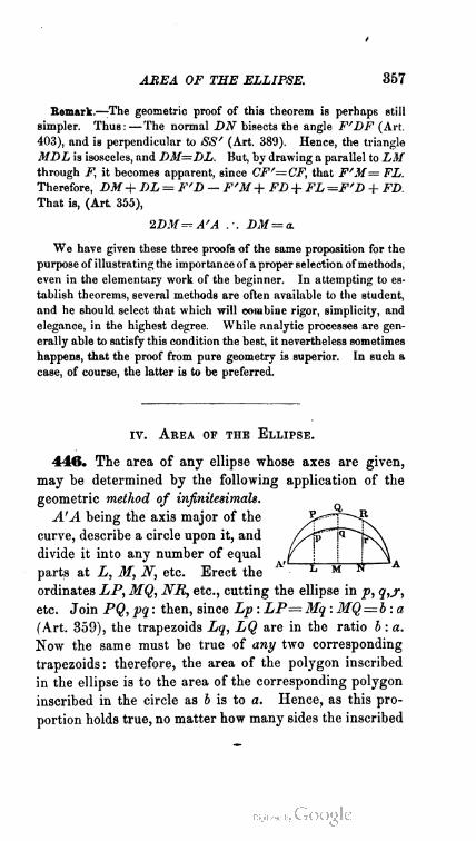
AREA OF THE ELLIPSE. 357
Remark.—The geometric proof of this theorem is perhaps still
simpler. Thus: — The normal DN bisects the angle F'DF (Art.
403), and is perpendicular to SS' (Art. 389). Hence, the triangle
MDL is isosceles, and DM=DL. But, by drawing a parallel to LM
through F, it becomes apparent, since CF/=CF, that F'M= FL.
Therefore, DM+DL = F'D — F'M+ FD+ FL =F'D + FD.
That is, (Art. 355),
IDM—A'A .-. DM=a.
We have given these three proofs of the same proposition for the
purpose of illustrating the importance of a proper selection ofmethods,
even in the elementary work of the beginner. In attempting to es
tablish theorems, several methods are often available to the student,
and he should select that which will combine rigor, simplicity, and
elegance, in the highest degree. While analytic processes are gen
erally able to satisfy this condition the best, it nevertheless sometimes
happens, that the proof from pure geometry is superior. In such a
case, of course, the latter is to be preferred.
iv. Area of the Ellipse.
446. The area of any ellipse whose axes are given,
may be determined by the following application of the
geometric method of infinitesimals.
A'A being the axis major of the
curve, describe a circle upon it, and
divide it into any number of equal
parts at L, M, N, etc. Erect the
ordinates LP, MQ, NR, etc., cutting the ellipse in p, q,jr,
etc. Join PQ, pq : then, since Lp : LP= Mq : MQ= b:a
(Art. 359), the trapezoids Lq, LQ are in the ratio b : a.
Now the same must be true of any two corresponding
trapezoids: therefore, the area of the polygon inscribed
in the ellipse is to the area of the corresponding polygon
inscribed in the circle as b is to a. Hence, as this pro
portion holds true, no matter how many sides the inscribed
358 ANALYTIC GEOMETRY.
polygons may have, and as we can make the number of
sides as great as we please by continually subdividing
the axis major, in the limiting case where the polygons
vanish into their respective curves, we shall have area
of ellipse : area of circumscribed circle — b:a. Now
(Geom., 500) the area of the circle = na2. Therefore,
putting A = the required area,
A — Ttab.
That is,
Theorem LIII.—The area of an ellipse is equal to it times
the rectangle under ils semi-axes.
Corollary.—Since rrab = VTia2. >-6", we have the addi
tional property : The area of an ellipse is a geometric
mean between the areas of its circumscribed and inscribed
circles.
EXAMPLES ON THE ELLIPSE.
1. Find the equations to the tangent and normal at the extremity
of the latus rectum, and determine the eccentricity of the ellipse in
which the normal mentioned passes through the extremity of the
axis minor.
2. Find the equations to the diameter passing through the ex
tremity of the latus rectum, and the chord joining the extremities
of the axes ; and determine the eccentricity of the ellipse in which
these lines are parallel.
3. A point P is so taken on the normal of an ellipse, that its
distance from the foot of the normal is in a constant ratio to the
length of the normal: find the locus of P, and prove that when P
is the middle point of the normal, its locus is an ellipse whose eccen
tricity e' is connected with that of the given one by the condition
(1— erl){\ + elf=\ — e\
4. Prove that two ellipses of equal eccentricity and parallel axes
can have only two points in common. Also, show that if three such
ellipses intersect, their three common chords will meet in one point.

EXAMPLES ON THE ELLIPSE. 359
5. If two parallels be drawn, one from an extremity A of the
axis major, and the other from the adjacent focus, meeting the axis
minor in M and N, the circle described from N as a center, with a
radius equal to MA, will either touch the ellipse or fall entirely
outside of it.
6. A circle is inscribed in the triangle formed by the axis major
and any two focal radii: find the locus of its center.
7. Find a point on an ellipse, such that the tangent there may
be equally inclined to both axes. Also, a point such that the tangent
may form upon the axes intercepts proportional to them.
8. Prove that the circle described on any focal radius of an ellipse
touches the circumscribed circle.
9. From the vertex of an ellipse a chord is drawn to any point
on the curve, and the parallel diameter is also drawn : the locus
of the intersection of this diameter and the tangent at the extrem
ity of the chord, is the tangent at the opposite vertex.
10. From the center of an ellipse, two radii vectores are drawn
at right angles to each other, and tangents to the curve are formed
at their extremities: the tangents intersect on the ellipse
^ , .V2 _ 1_ , Ia* "t" 6* a- + b* '
11. Two ellipses have a common center, and axes coincident in
direction, while the sum of the squares on the axes is the same in
both: find the equation to a common tangent.
12. The ordinate of any point P on an ellipse is produced to
meet the circumscribed circle in Q : the focal perpendicular upon
the tangent at Q is equal to the focal distance of P.
13. The lines which join transversely the foci and the feet of the
focal perpendiculars on any tangent, intersect on the corresponding
normal, and bisect it.
14. If a right line drawn from the focus of an ellipse meets the
tangent at a constant angle 6, the locus of its foot is a circle, which
touches the curve or falls entirely outside of it according as cos 6 is
less or greater than e.
15. When the angle between a tangent and its focal radius of
contact is least, the radius = a; and when the angle between a
tangent and its central radius of contact is least, the radius =
\ Vd' + b\
360 ANALYTIC GEOMETRY.
16. The locus of the foot of the central perpendicular upon any
tangent to an ellipse, is the curve
p2 = a' cos," 8 -f h2 sin2 d.
17. The locus of the variable intersection of two circles described
on two conjugate semi-diameters of an ellipse, is the curve
2p2 = a2 cos2 0 + 42sin20.
18. If lines drawn through any point of an ellipse to the extrem
ities of any diameter meet the conjugate CD in M and N, prove
that CM.CN= CD2.
19. In an ellipse, the rectangle under the central perpendicular
upon any tangent and the part of the corresponding normal inter
cepted between the axes, is constant, and equal to a2— 6s.
20. The condition that two diameters of an ellipse may be conju
gate, referred to a pair of conj ugates as axes of co-ordinates, is
bn
tan 8 tan & =— -p. ■
a1
21. Normals at P and D, the extremities of conjugate diameters,
meet in Q: prove that the diameter CQ is perpendicular to PD,
and find the locus of its intersection with the latter.
22. Given any two semi-diameters, if from the extremity of each
an ordinate be drawn to the other, the triangles so formed will be
equal in area. Also, if tangents be drawn at the extremity of each,
the triangles so formed will be equal in area.
23. Find the locus of the intersection of the focal perpendicular
upon any tangent with the radius vector from the center to the point
of contact. Also, the locus of the intersection of the central perpen
dicular with the radius vector from the focus to the point of contact.
24. The equi-conjugates being taken for axes, find the equation
to the normal at P, and prove that the normal bisects the line
joining the feet of the perpendiculars dropped from P upon the
equi-conjugates.
25. Find the locus of the intei-section of tangents drawn through
the extremities of conjugate diameters.
26. Putting p, p' to denote the focal radii of any point on an
ellipse, and <j> for its eccentric angle, prove that
p = a(l — «cos0), p' = a(l + ecos0).

EXAMPLES ON THE ELLIPSE. 361
27. Express the lengths of two conjugate semi-diameters in terms
of the eccentric angle, namely, by
a" — a2 cos2 (j> + V sin2 <j>, bn — a2 sin2 <p + ^2 cos2 <j>.
28. The ordinate MP of an ellipse being produced to meet the
circumscribed circle in Q, find the locus of the intersection of the
radius CQ with the focal radius FP.
29. Normals to the ellipse and circumscribed circle pass through
the points P and Q just mentioned, and intersect in It : find the
locus of It.
[First show that the equation to the normal of the ellipse is
ax _ _h_ _ 2
cos0 sin0 '
<p being the eccentric angle of the point of contact.]
30. Prove that the area of any parallelogram circumscribed
about an ellipse may be expressed by
4abarea = ——; — ,
sin (0 — '
where 0, are the eccentric angles corresponding to the points of
contact of the adjacent sides. Show that this area is least when
the points of contact are the extremities of conjugates.
31. Upon the axis major of an ellipse, two supplemental chords
are erected, and perpendiculars are drawn to them from the vertices :
show that the locus of the intersection of these perpendiculars is
another ellipse, and find its axes.
32. Let CP, CD be any two conjugate semi-diameters: the
supplemental chords from P to the extremities of any diameter are
parallel to those from D to the extremities of the conjugate.
33. The rectangle under the segments of any focal chord is to
the whole chord in a constant ratio.
34. The sum of two focal chords drawn parallel to two conjugate
diameters is constant.
35. The sum of the reciprocals of two focal chords at right angles
to each other is constant.
36. To a series of confocal ellipses, tangents are drawn from a
fixed point on the axis major : find the locus of the points of contact.
362 ANALYTIC GEOMETRY.
37. Tangents to two confocal ellipses are drawn to cut each other
at right angles: the locus of their intersection is a circle concentric
with the ellipses.
38. Find the sum of the focal perpendiculars upon the polar
of xy.
39. The intercept formed on any variable tangent by two fixed
tangents, subtends a constant angle at the focus. Also, the line
which joins the focus to the point in which any chord cuts the
directrix, is the external bisector of the focal angle subtended by
the chord.
40. One vertex of a circumscribed parallelogram moves along
one directrix of an ellipse : prove that the opposite vertex moves
along the other, and that the two remaining vertices move upon the
circumscribed circle.
CHAPTER FOURTH.
THE HYPERBOLA.
i. The Curve referred to its Axes.
44% In discussing the Hyperbola by means of its
equation (Art. 167)
ar y2 1
a% ~~ ¥ = '
we shall avoid the repetition of much that has already
been said in connection with the Ellipse, by considering
that the similarity of the equations to these two curves
makes most of the arguments used in the foregoing pages
at once applicable to the Hyperbola. We shall therefore
avail ourselves of the principle developed in the corollary
to Art. 167, and, for details, shall refer the student to
the proper article in the preceding Chapter.
For the sake of bringing out the antithesis between
the Ellipse and Hyperbola, alluded to in the Remark

PROPERTIES OF THE HYPERBOLA. 363
under Art. 167, the theorems of this Chapter are num
bered like the corresponding ones of the preceding.
THE AXES.
448. Making y and x successively equal to zero in
the equation of Art. 167, we get, for the intercepts of
the Hyperbola upon the lines termed its axes,
x—±a, y=±b V— 1.
Hence, the curve cuts the transverse axis in two real
points equally distant from the focal center, and the
conjugate axis in two imaginary points situated on
opposite sides of that center at the distance b j/— 1.
Assuming, then, the conjugate axis to be measured by
the imaginary unit V— 1, we may infer
Theorem I.—The focal center of any hyperbola bisects
the transverse axis, and also the conjugate.
Corollary.—In the light of the analysis leading to this
theorem, we should therefore interpret the constants a
and b in the equation
a2 b2~
as respectively denoting half the transverse axis and
half the modulus of the imaginary conjugate axis.
440. At the outset (see Art. 166.), we arbitrarily
used the phrase conjugate axis to
denote the whole line drawn through
the center 0 at right angles to the
transverse axis A'A. We now see
that the phrase in strictness means
an imaginary portion of that line,
of the length — 2b V^—i.
But, as was promised in Art. 166, we shall now show

364 ANALYTIC GEOMETRY.
that a certain real portion of this line has a most signifi
cant relation to the Hyperbola, on account of which it is
by universal consent taken- for the conjugate axis. This
relation depends on the companion-curve called the conju
gate hyperbola, whose equation we developed in Art. 168.
By referring to the close of Art. 168, it will be seen
that the equations to two conjugate hyperbolas, when
referred to their common center and axes, differ only in
the sign of the constant term. The equation to the curve
whose branches lie one above and the other below the
line A'A in the diagram, may therefore be written
Now, if in this we make x = 0, we get
y = ±b.
Hence, the conjugate hyperbola has a real axis, identical
in direction with the imaginary axis of the primary curve,
whose length is the same multiple of 1 that the length
of the imaginary is of V—1. Moreover, it is found that
this real axis of the conjugate hyperbola, when used in
stead of the imaginary one of the primary curve, enables
us to state the properties of the latter in complete analogy
to those of the Ellipse. It is customary, therefore, to lay
off CB, OB' each equal to b, and to treat the resulting
line B'B as the conjugate axis of the original hyperbola,
though in fact it is only the transverse axis of the conju
gate curve.
Adopting this convention, the statement in Theorem I
is to be taken without reference to imaginary quantities,
and the constants a and b in the equations
t. _ t.— -4-1
a2 b*

CONSTRUCTION OF CURVE AND FOCI. 365
are henceforth to be interpreted as denoting the semi-axes
of the curve.
450. If in the equation of Art. 167, which may be
written
b ,y = ±- Vx2 - d\
€1/
we suppose x < a or > — a, the corresponding values
of y are imaginary ; so that no point of the curve is
nearer to the origin, either on the right or on the left,
than the extremities of the transverse axis. But (Art.
171), for the distance from the origin to either focus,
we have
<? = a2 + b2.
Hence, c can not be less than a, though it may approach
infinitely near to the value of a, as b diminishes toward
zero. Therefore,
Theorem II.—The foci of any hyperbola fall without
the curve.
451. Moreover, c — a measures the distance of either
focus from the adjacent vertex; while the distance of
either from the remote vertex = c + a. Hence,
Theorem III.—The vertices of the curve are equally
distant from the foci.
452. From Art. 448, the length of the transverse
axis = 2a. But (Art. 167) 2a = the constant difference
of the focal radii of any point on the curve. That is,
Theorem IV.— The difference of the focal radii of any
point on an hyperbola is equal to the length of its trans
verse axis.
Corollary.—We may therefore construct the curve by
points as follows:—From either focus, as F', lay off
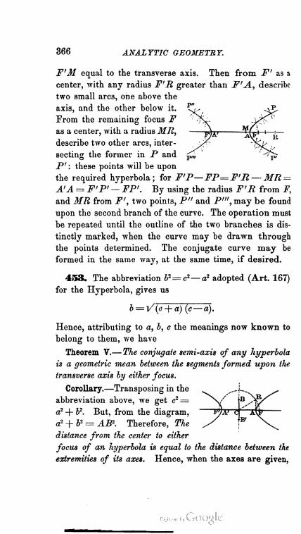
366 ANALYTIC GEOMETRY.
F'M equal to the transverse axis. Then from F' as a
center, with any radius F'R greater than F'A, describe
two small arcs, one above the
axis, and the other below it.
From the remaining focus F
as a center, with a radius MR,
describe two other arcs, inter
secting the former in P and
P' : these points will be upon
the required hyperbola; for F'P—FP-^F'R— 31R =
A'A = F'P' — FP'. By using the radius F'R from F,
and MR from F', two points, P" and P'", may be found
upon the second branch of the curve. The operation must
be repeated until the outline of the two branches is dis
tinctly marked, when the curve may be drawn through
the points determined. The conjugate curve may be
formed in the same way, at the same time, if desired.
453. The abbreviation b2—c2— a2 adopted (Art. 167)
for the Hyperbola, gives us
b = V(o + a) (c— a).
Hence, attributing to a, b, c the meanings now known to
belong to them, we have
Theorem V.—The conjugate semi-axis of any hyperbola
is a geometric mean between the segments formed upon the
transverse axis by either focus.
Corollary.—Transposing in the
abbreviation above, we get c2 =
a2 + b2. But, from the diagram,
a? + b2 = AB?. Therefore, The
distance from the center to either
focus of an hyperbola is equal to the distance between the
extremities of its axes. Hence, when the axes are given,

LATUS RECTUM OF HYPERBOLA. 367
we may construct the foci as follows : — From the center C,
with a radius equal to the diagonal of the rectangle under
the semi-axes, describe an arc cutting the transverse axis
produced in F and F' : the two points of intersection will
be the foci sought.
4*54. By an analysis similar to that of Art. 357, the
details of which the student must supply,* we obtain
Theorem VI.—The squares on the ordinates drawn to
either axis of an hyperbola are proportional to the rect
angles under the corresponding segments of that axis.
Corollary.—For the ordinate passing through .either
focus, we shall therefore have
h2 *\ 9
But c2—a2=b2. Hence, doubling
FP or F'P',
latus rectum = — = „ ^ .
a la
That is, The latus rectum of any hyperbola is a third
proportional to the transverse axis and the conjugate.
455. Throwing the equations to the Hyperbola and
its conjugate into the forms
y2 b2 x2 a2
{x+a) {x-a) = a2 ' (y + b) (y - b)=P '
we at once obtain
Theorem VII.—The squares on the axes of any hyperbola
are to each other as the rectangle under any two segments
of either is to the square on the ordinate which forms the
segments.
KWhen seeking properties of the conjugate axis, we must of course uso
tho equation to the conjugate hyperbola.
An. Ge. 34.
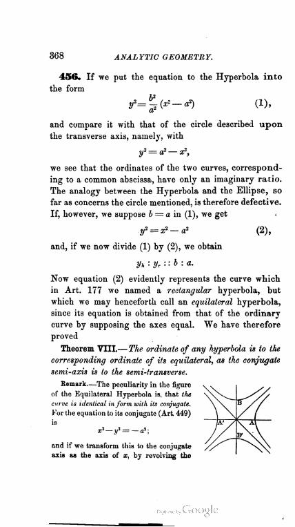
368 ANALYTIC GEOMETRY.
456. If we put the equation to the Hyperbola into
the form
and compare it with that of the circle described upon
the transverse axis, namely, with
y2=a? — x2,
we see that the ordinates of the two curves, correspond
ing to a common abscissa, have only an imaginary ratio.
The analogy between the Hyperbola and the Ellipse, so
far as concerns the circle mentioned, is therefore defective.
If, however, we suppose b = a in (1), we get
y* = x>-a* (2),
and, if we now divide (1) by (2), we obtain
yh: yr::b : a.
Now equation (2) evidently represents the curve which
in Art. 177 we named a rectangular hyperbola, but
which we may henceforth call an equilateral hyperbola,
since its equation is obtained from that of the ordinary
curve by supposing the axes equal. We have therefore
proved
Theorem VIII.—The ordinate of any hyperbola is to the
corresponding ordinate of its equilateral, as the conjugate
semi-axis is to the semi-transverse.
Kemark—The peculiarity in the figure
of the Equilateral Hyperbola is, that the
curve is identical in form with its conjugate.
For the equation to its conjugate (Art 449)
is
x2— y2 = — a2;
and if we transform this to the conjugate
axis as the axis of x, by revolving the

EQUILATERAL HYPERBOLA. 369
reference-axes through 90°, and therefore (Art. 56, Cor. 3) replacing
a; by — y, and y by x, we obtain
so that the conjugate curve, when referred to its own transverse
axis, is represented by the same equation as its primary, and is
therefore the same curve. The diagram presents a pair of conjugate
equilaterals.
Corollary.—Notwithstanding the defective analogy be
tween the Ellipse and the Hyperbola with respect to the
circle formed upon the transverse axis, this curve still
aids us in fixing the meaning of the abbreviation
adopted in Art. 170, and warrants us in calling e the
eccentricity of the Hyperbola. For, as in the case of the
Ellipse, since ar + b2 = c2, we learn that e is the ratio
which the distance from the center to either focus of an
hyperbola bears to its transverse semi-axis. Let us, then,
suppose a series of ellipses and hyperbolas to be described
upon a common transverse
axis: we saw (Art. 359,
Cor. 2) that, as the vary
ing ellipse of such a series
deviates more and more
from the circle formed
upon the same axis, and
approaches nearer and nearer to coincidence with the
axis A'A, the eccentricity e advances nearer and nearer
to the limit 1. Assuming, then, that e actually reaches
this limit, the corresponding ellipse must vanish into the
line A'A, which forms the common axis. Now, from the
abbreviation above, the e of the Hyperbola lies between
the limits 1 and co : hence the series of hyperbolas may
be said to arise out of the common axis A'A at the

370 ANALYTIC GEOMETRY.
instant when the series of ellipses vanishes into it, and
to recede farther and farther from the axis as e advances
from 1 toward oo. But since e, with respect to the ellipses
and the hyperbolas both, is at all times the ratio between
the same elements of the curves ; and since, taking the circle
described upon the common axis as the starting-point, this
ratio steadily advances from 0 through 1 toward oo; we
may regard the recession of the hyperbolas from the axis
A'A as a farther deviation from the curvature of the circle
mentioned, and consequently call e, which measures this
deviation, the eccentricity.
We may therefore interpret the name hyperbola (derived
from the Greek urrsofid/j.siu, to exceed) as signifying, that,
in this curve, the eccentricity is greater than unity.
Since e increases as b increases, it follows that the
greater the eccentricity, the more obtuse will be the
branches of the corresponding hyperbola. In case the
curve is equilateral, or b — a, we shall have
e = V2.
457. The distance of any point on an hyperbola from
either focus, may be expressed in terms of the abscissa
of the point. For, putting p to denote any such focal
distance, we have (Art. 167)
P*=(x±cy+f.
Substituting for y2 from the equation to the curve, and
reducing by means of the relations in Art. 171, we get
p = ex ± a,
where the upper sign corresponds to the left-hand focus,
and the lower to the right-hand one. Hence,
Theorem IX.—The focal radius of any point on an
hyperbola is a linear function of the corresponding abscissa.
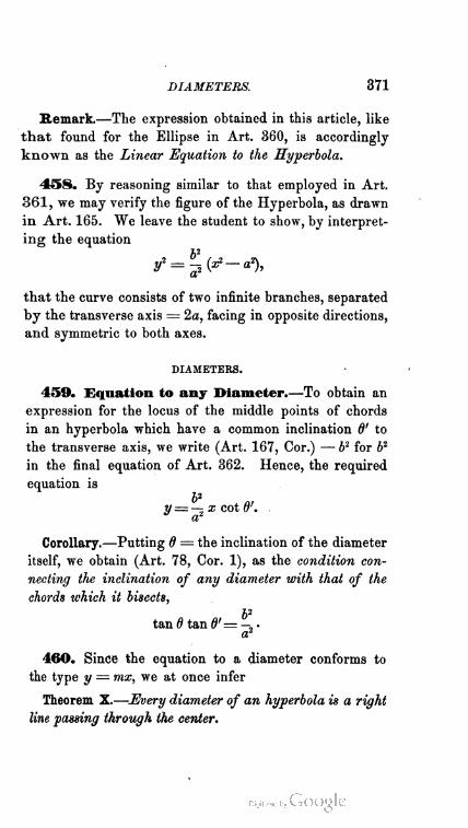
DIAMETERS. 371
Remark.—The expression obtained in this article, like
that found for the Ellipse in Art. 360, is accordingly
known as the Linear Equation to the Hyperbola.
458. By reasoning similar to that employed in Art.
361, we may verify the figure of the Hyperbola, as drawn
in Art. 165. We leave the student to show, by interpret
ing the equation
that the curve consists of two infinite branches, separated
by the transverse axis = 2a, facing in opposite directions,
and symmetric to both axes.
DIAMETERS.
459. Equation to any Diameter.—To obtain an
expression for the locus of the middle points of chords
in an hyperbola which have a common inclination d' to
the transverse axis, we write (Art. 167, Cor.) — b2 for b2
in the final equation of Art. 362. Hence, the required
equation is
b2y =— x cot 0'.
a~
Corollary.—Putting 6 = the inclination of the diameter
itself, we obtain (Art. 78, Cor. 1), as the condition con
necting the inclination of any diameter with that of the
chords which it bisects,
b2tan d tan d'= — •
a2
46©. Since the equation to a diameter conforms to
the type y = mx, we at once infer
Theorem X.—-Every diameter of an hyperbola is a right
line passing through the center.
372 ANALYTIC GEOMETRY.
Corollary.—The angle 01 being arbitrary, it follows
from the above condition, that d is also arbitrary.
Hence the converse theorem : Every right line that
passes through the center of an hyperbola is a diameter.
461. Eliminating, then, between the equation
y — x tan d
and the equation to the Hyperbola, we get, for the
abscissas of intersection between the curve and any
diameter, ,ab
x~ — V'(b2 — a2 tan2 W) '
Now these abscissas evidently become imaginary when
a2 tan2 1) > b2. Hence,
Theorem XI.—The proposition that every diameter cuts
the curve in two real points, is not true of the Hyperbola.
Corollary 1.—It is obvious, however, that the intersec
tions will be real, and at a finite distance from the center,
so long as a1 tan' d < b2. Hence, the diameters corre
sponding to a2 tan2 d = b2, that is, the two diameters
whose tangents of inclination are respectively
tan 0 — — , tan d' = — — ,
a a
form the limits between those diameters which have real
intersections with the curve and those which have not.
But, from the values of their tangents of inclination,
these two diameters are the diagonals of the rectangle
contained by the axes. We learn, then, that diameters
which cut the Hyperbola in real points must either
make with the transverse axis an angle less than is made
by the first of these diagonals, or greater than is made by
the second.

LENGTH OF DIAMETER. 373
It deserves notice, that the condition a2 tan2 0 = b2
renders the abscissas of intersection, as expressed above,
infinite. The two limiting diameters therefore meet the
curve at infinity: and we have come upon the analogue
of the equi-conjugates in the Ellipse. We shall soon
find that these lines are the most remarkable elements
of the Hyperbola, giving it a series of properties in
which the other Conies do not share.
Corollary 2.—Eliminating between y — x tan d and the
equation to the conjugate hyperbola, we get
abx~ — j/ (a2 tan2 0 — b2) '
Here, then, the condition of real intersection is a2tan20>62.
Hence, Every diameter that cuts an hyperbola in two imag
inary points, cuts its conjugate in two real ones.
462. Length ofany Diameter.—This being double
the central radius vector of the curve, may be determined
(Art. 170) by ,2
2 •
P = e2 cos2 0 — 1 '
or, if the diameter meets the conjugate curve instead of
the primary, by ,2
2
9 ~ 1 — e2 cos2 0 '
an expression readily obtained by transforming to polar
co-ordinates (Art. 57, Cor.) the equation to the conjugate
hyperbola, found in Art. 449.
463. The first of the above expressions is least when
6 = 0; and the second, when 0 = 90°. Hence,
Theorem XII.—Each axis is the minimum diameter of
its own curve.
Remark.—We see, then, that the terms major and minor
are not applicable to the axes of an hyperbola.
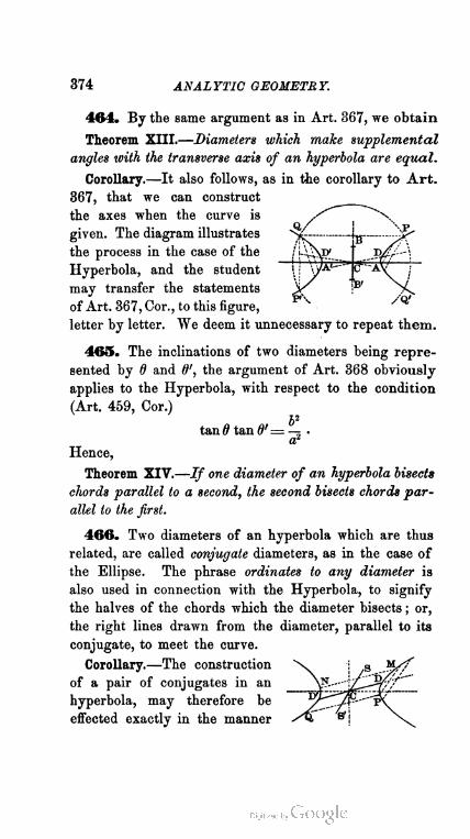
374 ANALYTIC GEOMETRY.
464. By the same argument as in Art. 367, we obtain
Theorem XIII.—Diameters which make supplemental
angles icith the transverse axis of an hyperbola are equal.
Corollary.—It also follows, as in the corollary to Art.
367, that we can construct
the axes when the curve is
given. The diagram illustrates
the process in the case of the
Hyperbola, and the student
may transfer the statements
of Art. 367, Cor., to this figure,
letter by letter. We deem it unnecessary to repeat them.
465. The inclinations of two diameters being repre
sented by 0 and 0', the argument of Art. 368 obviously
applies to the Hyperbola, with respect to the condition
(Art. 459, Cor.)
b2
tan 0 tan
a'
Hence,
Theorem XIV.—If one diameter of an hyperbola bisects
chords parallel to a second, the second bisects chords par
allel to the first.
466. Two diameters of an hyperbola which are thus
related, are called conjugate diameters, as in the case of
the Ellipse. The phrase ordinates to any diameter is
also used in connection with the Hyperbola, to signify
the halves of the chords which the diameter bisects ; or,
the right lines drawn from the diameter, parallel to its
conjugate, to meet the curve.
Corollary.—The construction \ i a m>
of a pair of conjugates in an
hyperbola, may therefore be
effected exactly in the manner

CONJUGATE DIAMETERS. 375
described in the corollary to Art. 369. The details may
be gathered by applying to the parts of the annexed
diagram, the statements of that corollary.
467. Equation of Condition for Conjugates in
tlie Hyperbola.—The conjugate of any diameter being
parallel to the chords which the diameter bisects, the in
clinations of two conjugates must be connected in the
same way as those of a diameter and its ordinates.
Hence, if 6 and 6' represent the inclinations, the re
quired condition (Art. 459, Cor.) is
b2tan 6 tan 6'= —.-
a2
Corollary.—Hence, if tan 0 < & : a, tan d'^>b : a; and
if tan d > — b : a, tan 6' < — b : a. Therefore (Art. 461,
Cors. 1, 2), If one of two conjugates meets an hyperbola,
the other meets the conjugate curve.
Bemark.—The condition of this article might have heen obtained
from that of Art. 370, by merely changing b2 into — b1.
468. The preceding condition shows that the tangents
of inclination have like signs. Hence, the angles made
with the transverse axis by two conjugates are either
both acute, or else both obtuse. That is,
Theorem XV.—Conjugate diameters of an hyperbola lie
on the, same side of the conjugate axis.
469. Equation to a Diameter conjugate to a
Fixed Point.—Making the requisite change of sign
(Art. 167, Cor.) in the equation of Art. 372, we get the
one now sought, namely,
— _ tl — n
a2 ¥ ~
An. Ge. 35.

376 ANALYTIC GEOMETRY.
Corollary.—The diameter conjugate to that which
passes through {a, 0) is therefore x = 0, that is, the
conjugate axis. Hence, The axes of an hyperbola con
stitute a case of conjugate diameters.
470. Problem.—Given the co-ordinates of the extrem
ity of a diameter, to find those of the extremity of its
conjugate.
By the extremities of the conjugate diameter, are
meant the points in which the conjugate cuts the conju
gate hyperbola. The required co-ordinates are therefore
found by eliminating between the equation of Art. 469
and
They are
- , ay' , bx1xc= ±-%-, yc=± — .
o a
Remark.—By comparing these expressions with those
of Art. 373, we notice that the abscissa and ordinate of
the conjugate diameter in the Ellipse have opposite signs,
but in the Hyperbola like signs. This agrees with the
properties developed in Arts. 371, 468.
471. The equations of Art. 470, like those of Art. 373, give
rise to
Theorem XVI.—The abscissa of the extremity of any diameter is
to the ordinate of the extremity of its conjugate, as the transverse axis
is to the conjugate axis.
473. By following, with respect to the second ex
pression of Art. 470, the steps indicated in Art. 375,
excepting that we subtract the yn, we arrive at
Theorem XVII.—The difference of the squares on the
ordinates of the extremities of conjugate diameters is con
stant, and equal to the square on the conjugate semi-axis.

LENGTH OF CONJUGATES. 377
Remark.—We leave the student to prove the analogous
property : The difference of the squares on the abscissas
of the extremities of conjugate diameters is constant, and
equal to the square on the transverse semi-axis.
473. Problem.— To find the length of a diameter in
terms of the abscissa of the extremity of its conjugate.
Let x'y' be the extremity of any diameter, a' half its
length, and V half the length of its conjugate. Then
a'2 = x12 + yn, and we get (Art. 470)
«'2- ai V? + ^ W+ a*) + %
since xc and yc must satisfy the equation to the conjugate
hyperbola. Hence, (Art. 171,)
a'2 = e2x2 -f- a2.
By performing similar operations with respect to b', we
should get
b'2 = e2x'2—a2.
474. Between these results and those of Art. 376,
there is a striking difference ; and, as only the value of
b'2 equals (Art. 457) the rectangle of the focal radii
drawn to x'y', it appears as if the property proved of
the Ellipse in Art. 377 were only true of the Hyperbola
with respect to those diameters which meet the conju
gate curve instead of the primary. But when we reflect
that it is entirely arbitrary which of two conjugate hyper
bolas we consider the primary, it becomes evident that
the property of Art. 377 is also true of the diameters
which meet the curve hitherto called the primary, pro
vided we suppose the focal radii in question to be drawn
from the foci of the conjugate curve. With this under
standing, then, we may state
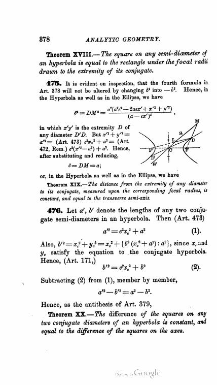
378 ANALYTIC GEOMETRY.
Theorem XVIII.—The square on any semi-diameter of
an hyperbola is equal to the rectangle under thefocal radii
drawn to the extremity of its conjugate.
475. It is evident on inspection, that the fourth formula in
Art. 378 will not be altered by changing b1 into — b2. Hence, in
the Hyperbola as well as in the Ellipse, we have
(a — ex')'
in which x'y' is the extremity D of
any diameter Z/D. But x'1 + y'2 =
an= (Art. 473) Ace* + a1= (Art.
472, Rem.) e\3/1— dl) + a\ Hence,
after substituting and reducing,
6=DM=a;
or, in the Hyperbola as well as in the Ellipse, we have
Theorem XIX.—The distance from the extremity of any diameter
to its conjugate, measured upon the corresponding focal radius, is
constant, and equal to the transverse semi-axis.
476. Let a', b' denote the lengths of any two conju
gate semi-diameters in an hyperbola. Then (Art. 473)
an= e2x? + a? (1).
Also, b'2— xc2-\- y? = %?Jc {b2 (x2 + a2) : a2}, since £rand
ye satisfy the equation to the conjugate hyperbola.
Hence, (Art. 171,)
6'J = eV + b2 (2).
Subtracting (2) from (1), member by member,
Hence, as the antithesis of Art. 379,
Theorem XX.—The difference of the squares on any
two conjugate diameters of an hyperbola is constant, and
equal to the difference of the squares on the axes.
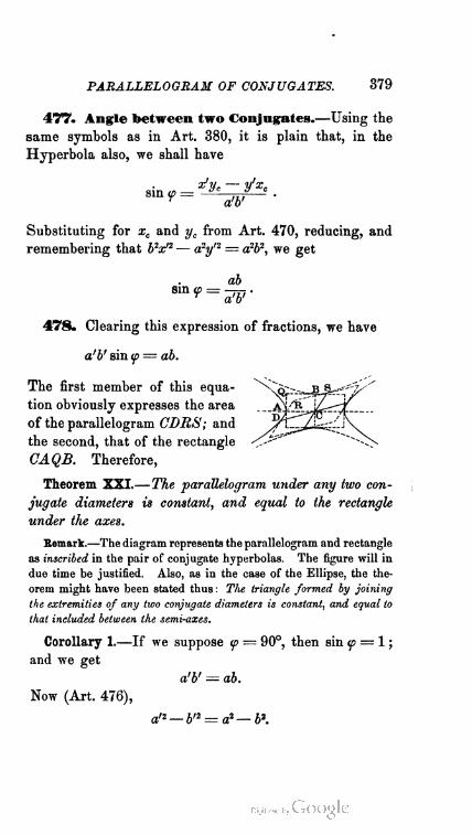
PARALLELOGRAM OF CONJUGATES. 379
47"7. Angle between two Conjngates.—Using the
same symbols as in Art. 380, it is plain that, in the
Hyperbola also, we shall have
Substituting for xc and yc from Art. 470, reducing, and
remembering that b2x'2 — dry'2 = a2b2, we get
478. Clearing this expression of fractions, we have
a'b' sin f = ab.
CAQB. Therefore,
Theorem XXI.—The parallelogram under any two con
jugate diameters is constant, and equal to the rectangle
under the axes.
Remark.—The diagram represents the parallelogram and rectangle
as inscribed in the pair of conjugate hyperbolas. The figure will in
due time be justified. Also, as in the case of the Ellipse, the the
orem might have been stated thus : The. triangle formed by joining
the extremities of any two conjugate diameters is constant, and equal to
that included between the semi-axes.
Corollary 1.—If we suppose <p = 90°, then sin <p = 1 ;
and we get
sin f --x'yc — y%
a'b'
ab
The first member of this equa
tion obviously expresses the area
of the parallelogram CDRS; and
the second, that of the rectangle
a'■!V — ab.
Now (Art. 476),
a'2 — b'2 = a2 — b2.

380 ANALYTIC GEOMETRY.
Solving these equations for a' and b', we find, as the only
real values,
a' — a, b' = b.
Therefore, In any hyperbola there is but one pair of eon-
jugate diameters at right angles to each other, namely, the
axes.
Corollary 2.—We saw (Arts. 381, Cor. 1 ; 382, Cor.)
that, in the Ellipse, sin <p lies between the limits 1 and
2ab : (a2 + b2). But (Art. 476), a'2 = b'2 + constant, in the
Hyperbola: whence a' and V must increase or diminish
together. Therefore, as any diameter (Art. 461, Cor. 1)
tends toward an infinite length the nearer its inclination
approaches the limit 0 = tan-1 6 : a, the semi-conjugates
a' and ¥ must advance together toward the value oo, and
the product a'V tends toward oo for its maximum. That
is, sin <p tends toward the limit 0 ; or, The angle between
two conjugates in an hyperbola diminishes without limit.
But though the conjugates thus tend to final coinci
dence as each tends to an infinite length, the relation
a'2 — b'2 = constant renders it impossible that the condi
tion a' — V shall ever arise in the Hyperbola, unless
the curve is equilateral. The infinite diameters that
form the limit of the ever-approaching conjugates are
therefore not equal infinites, and the conception of
equi-conjugates is not in general present in the curve.
However, from the equation of condition for conjugate
diameters, namely,
b2tan# tan d'= —.,
a2
it is plain that when the conjugates finally coincide,
each makes with the transverse axis an angle whose
tangent is either b : a or else — b : a. Hence, the two
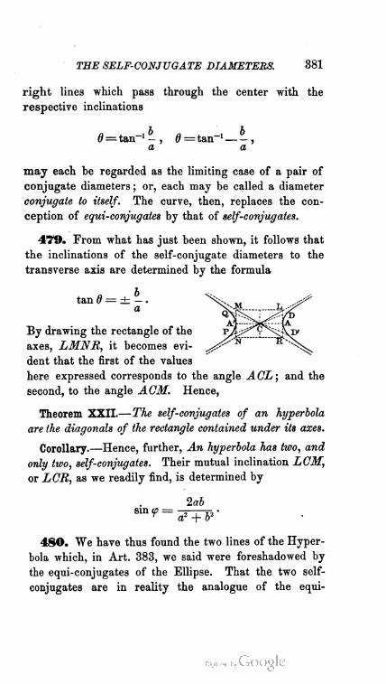
THE SELF-CONJUGATE DIAMETERS. 381
right lines which pass through the center with the
respective inclinations
0=^tan_1 — , 0=tan-1 — — ,
a a
may each be regarded as the limiting case of a pair of
conjugate diameters ; or, each may be called a diameter
conjugate to itself. The curve, then, replaces the con
ception of equi-conjugates by that of self-conjugates.
479. From what has just been shown, it follows that
the inclinations of the self-conjugate diameters to the
transverse axis are determined by the formula
tan 0 = ± - .
a
By drawing the rectangle of the
axes, LMNR, it becomes evi
dent that the first of the values
here expressed corresponds to the angle ACL; and the
second, to the angle ACM. Hence,
Theorem XXII.—The self-conjugates of an hyperbola
are the diagonals of the rectangle contained under its axes.
Corollary.—Hence, further, An hyperbola has two, and
only two, self-conjugates. Their mutual inclination LCM,
or LCR, as we readily find, is determined by
2ab
4SO. We have thus found the two lines of the Hyper
bola which, in Art. 383, we said were foreshadowed by
the equi-conjugates of the Ellipse. That the two self-
conjugates are in reality the analogue of the equi
382 ANALYTIC GEOMETRY.
conjugates, we can easily show : for though it is true,
as we saw in the second corollary to Art. 478, that the
two infinitely long conjugates which unite in either of
the self-conjugates are not equal infinites, still the two
self-conjugates, when compared with each other, are
equal infinites. For, since they make equal angles
ACL, ACR with the transverse axis, they are the
limiting case to which two equal diameters DP, D'Q
necessarily tend as their extremities D and D' move
along the curve in opposite directions from the vertex A.
But the chief interest of the self-conjugates is due to
a property in which the equi-conjugates of the Ellipse
have no share, and in virtue of which they are called
the asymptotes of the Hyperbola. From this property
are derived several others, peculiar to the latter curve,
which will receive a separate consideration in the proper
place.
THE TANGENT.
481. Equation to the Tangent.—To obtain this
for the Hyperbola, we simply change b2 into — b2 in the
equation of Art. 385. We thus get
7>x y'y _ 1
a2 62 — '
483. Condition that a Right Line shall touch
an Hyperbola.—Making the characteristic change of
sign in the condition of Art. 386, we have
11 = Vm2d2 — b2
as the condition that the line y — mx + n may touch
the curve
x2 y2
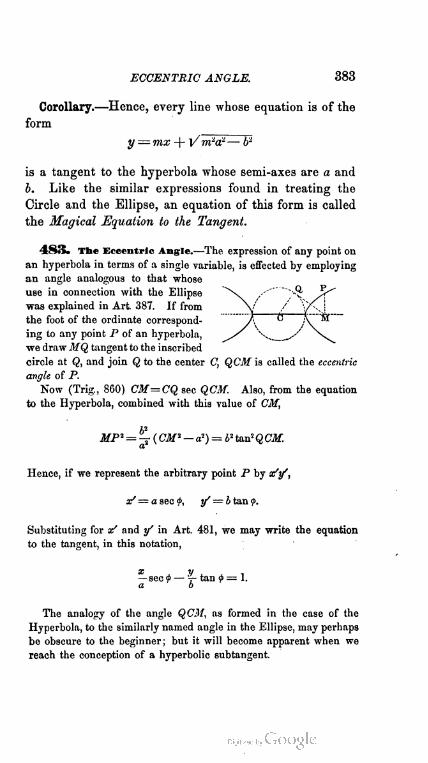
ECCENTRIC ANGLE. 383
Corollary.—Hence, every line whose equation is of the
form
y =mx -f- Vniidi— b3
is a tangent to the hyperbola whose semi-axes are a and
b. Like the similar expressions found in treating the
Circle and the Ellipse, an equation of this form is called
the Magical Equation to the Tangent.
483. The Eccentric Angle.—The expression of any point on
an hyperbola in terms of a single variable, is effected by employing
an angle analogous to that whose
U8e in connection with the Ellipse
was explained in Art. 387. If from
the foot of the ordinate correspond
ing to any point P of an hyperbola,
we draw MQ tangent to the inscribed
circle at Q, and join Q to the center C, QCM is called the eccentric
angle of P.
Now (Trig., 860) CM=CQ sec QCM. Also, from the equation
to the Hyperbola, combined with this value of CM,
MP2= ~( CM2 — a2) = 42 tan2 Q CM.
Hence, if we represent the arbitrary point P by x'y/,
x' — a sec <j>, y' — b tan <p.
Substituting for x' and y' in Art. 481, we may write the equation
to the tangent, in this notation,
x j. V i. a. i— sec <t> — t tan 0=1.a b
The analogy of the angle QCM, as formed in the case of the
Hyperbola, to the similarly named angle in the Ellipse, may perhaps
be obscure to the beginner; but it will become apparent when we
reach the conception of a hyperbolic subtangent.

•384 ANALYTIC GEOMETRY.
1
484. Problem.—If a tangent to an hyperbola posset
through a fixed point, to find the co-ordinates of contact.
Let x"y" be the fixed point, and x'y' the required
point of contact. Then, changing the sign of b2 in the
results of Art. 388, we get
, _ a2b2x" + a2y" Va2y"2— + a2°*
b2x"2— a2y"2 '
a2b2if ± b2x" Va2y"2 — b2x"2 + a2b2
y — b2x"2—a2y"2
Corollary 1.—The form of these values indicates that
from any given point two tangents can be drawn to an
hyperbola : real when a2y"2 — b2x"2 + a2b2 > 0, that is,
when the point is inside of the curve ; coincident when
ahf"2— b2x"2 + a2b2 — 0, that is, when the point is on the
curve ; imaginary when a2y" — b2x"2 + a2b2 < 0, that is,
when the point is outside of the curve.
Corollary 2.—With regard to any two real tangents
drawn from a given point, it is evident that their ab
scissas of contact will have like signs, if they both touch
the same branch of the curve, and unlike signs, if the
two touch different branches. But, if the two values of
x' above have like signs, then, merely numerical relations
being considered,
aW > a2y" Va2y"2—b2x"2 + a2b2\
that is, after squaring, transposing, and reducing,
y"<h-x".
a
Hence, as y — (b : a) x is the equation to the diagonal
of the rectangle formed upon the axes (Art. 461, Cor. 1),
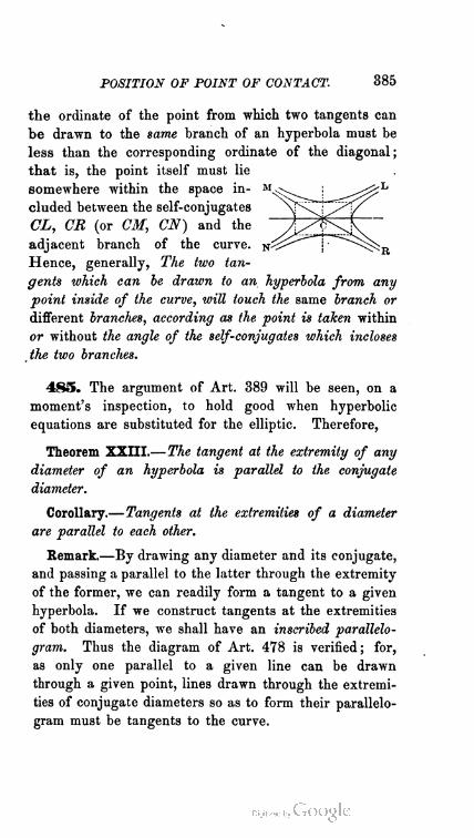
POSITION OF POINT OF CONTACT. 385
the ordinate of the point from which two tangents can
be drawn to the same branch of an hyperbola must be
less than the corresponding ordinate of the diagonal;
that is, the point itself must lie
somewhere within the space in- M,
eluded between the self-conjugates
CL, CR (or CM, CN) and the "
adjacent branch of the curve, n-'
Hence, generally, The two tan
gents which can be drawn to an hyperbola from any
point inside of the curve, will touch the same branch or
different branches, according as the point is taken within
or without the angle of the self-conjugates which incloses
the two branches.
485. The argument of Art. 389 will be seen, on a
moment's inspection, to hold good when hyperbolic
equations are substituted for the elliptic. Therefore,
Theorem XXIII.—The tangent at the extremity of any
diameter of an hyperbola is parallel to the conjugate
diameter.
Corollary.—Tangents at the extremities of a diameter
are parallel to each other.
Remark.—By drawing any diameter and its conjugate,
and passing a parallel to the latter through the extremity
of the former, we can readily form a tangent to a given
hyperbola. If we construct tangents at the extremities
of both diameters, we shall have an inscribed parallelo
gram. Thus the diagram of Art. 478 is verified; for,
as only one parallel to a given line can be drawn
through a given point, lines drawn through the extremi
ties of conjugate diameters so as to form their parallelo
gram must be tangents to the curve.
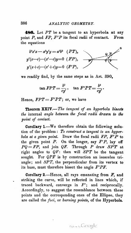
38G ANALYTIC GEOMETRY.
486. Let PT be a tangent to an hyperbola at any
point P, and FP, F'P its focal radii of contact. From
the equations
we readily find, by the same steps as in Art. 390,
tan FPT= , tan F'PT= —f .
cy cy'
Hence, FPT= F'PT; or, we have
Theorem XXIV.—The tangent of an hyperbola bisects
the internal angle between the focal radii drawn to the
point of contact.
Corollary 1.—We therefore obtain the following solu
tion of the problem : To construct a tangent to an hyper
bola at a given point. Draw the focal radii FP, F'P to
the given point P. On the longer, say F'P, lay off
PQ = FP, and join QF. Through P draw SPT at
right angles to QF: then will SPT be the tangent
sought. For QPF is by construction an isosceles tri
angle; and SPT, the perpendicular from its vertex to
its base, must therefore bisect the angle F'PF.
Corollary 2.—Hence, all rays emanating from F, and
striking the curve, will be reflected in lines which, if
traced backward, converge in F'; and reciprocally.
Accordingly, to suggest the resemblance between these
points and the corresponding ones of the Ellipse, they
are called the foci, or burning points, of the Hyperbola.
s
bix'x — a2y'y = a2b2 (PT),
y'(x-c)-(x'-c)y=Q (FP),
y'(x+c)-(x>+c)y=0 (F'P),
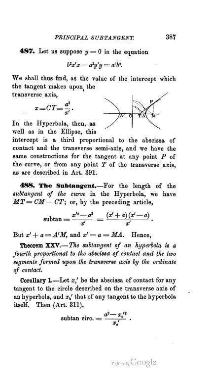
PRINCIPAL SUBTANGENT. 387
487. Let us suppose y — 0 in the equation
Vx'x— a2y'y = a2b2.
We shall thus find, as the value of the intercept which
the tangent makes upon^ the
transverse axis,
a2
x=CT=~.
In the Hyperbola, then, as
well as in the Ellipse, this
intercept is a third proportional to the abscissa of
contact and the transverse semi-axis, and we have the
same constructions for the tangent at any point P of
the curve, or from any point T of the transverse axis,
as are described in Art. 391.
488. The Subtangent.—For the length of the
subtangent of the curve in the Hyperbola, we have
MT= CM— CT; or, by the preceding article,
x'2— a2 (a/ + a)(af— a)
subtan = ;— = 5 ^ ' .x x
But x'+a= A'M, and x' — a — MA. Hence,
Theorem XXV.—The subtangent of an hyperbola is a
fourth proportional to the abscissa of contact and the two
segments formed upon the transverse axis by the ordinate
of contact.
Corollary 1.—Let xj be the abscissa of contact for any
tangent to the circle described on the transverse axis of
an hyperbola, and xh' that of any tangent to the hyperbola
itself. Then (Art. 311),
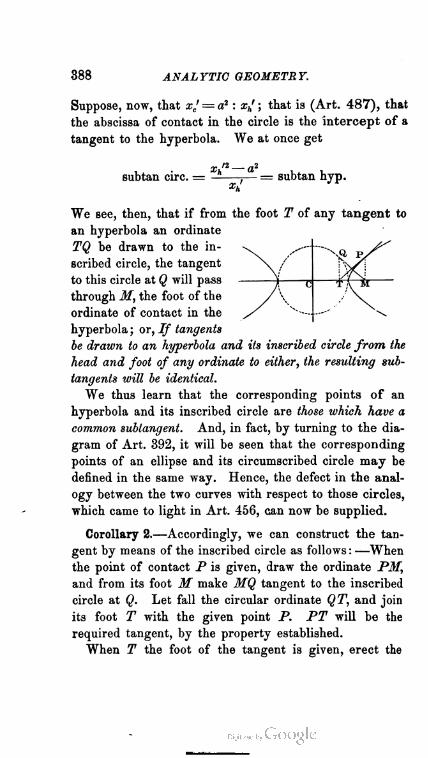
388 ANALYTIC GEOMETRY.
Suppose, now, that xj = a2 : xh' ; that is (Art. 487), that
the abscissa of contact in the circle is the intercept of a
tangent to the hyperbola. We at once get
We see, then, that if from the foot T of any tangent to
TQ be drawn to the in
scribed circle, the tangent
to this circle at Q will pass
through M, the foot of the
ordinate of contact in the
hyperbola ; or, If tangents
be drawn to an hyperbola and its inscribed circle from the
head and foot of any ordinate to either, the resulting sub-
tangents will be identical.
We thus learn that the corresponding points of an
hyperbola and its inscribed circle are those ivhich have a
common sublangent. And, in fact, by turning to the dia
gram of Art. 392, it will be seen that the corresponding
points of an ellipse and its circumscribed circle may be
defined in the same way. Hence, the defect in the anal
ogy between the two curves with respect to those circles,
which came to light in Art. 456, can now be supplied.
Corollary 2.—Accordingly, we can construct the tan
gent by means of the inscribed circle as follows : —When
the point of contact P is given, draw the ordinate P3I,
and from its foot M make MQ tangent to the inscribed
circle at Q. Let fall the circular ordinate QT, and join
its foot T with the given point P. PT will be the
required tangent, by the property established.
When T the foot of the tangent is given, erect the
subtan circ. =
= subtan hyp.
an hyperbola an ordinate
CENTRAL PERPENDICULAR ON TANGENT. 389
circular ordinate TQ, and draw the corresponding tan
gent QM. From M, the foot of this, erect the hyperbolic
ordinate MP, and join its extremity P with the given
point T.
Remark.—By comparing the diagrams of Arts. 387, 483 with
those of Art 392 and the present article, the complete analogy of
the eccentric angles in the two curves will, as we stated in Art. 483,
become apparent. The eccentric angle of any point on either curve,
may be defined as the central angle determined by the corresponding
point of the circle described upon the transverse axis, it being under
stood that the "corresponding" points are those which have a
common subtangent.
489. Perpendicular from the Center to any
Tangent.—The length of the perpendicular from the
origin upon the line
b2x'x — a2y'y — a2b2,
(Art. 92, Cor. 2) must be
— a2&2 _ ah
P ~ i/(b4x'2 + «y2) ~~ ^/(eV2— a2) '
Now (Art. 473) eV2— a2=6'2. Therefore,
ah
P=V->
or, as in the Ellipse, we have
Theorem XXVI.—The central perpendicular upon any
tangent of an hyperbola is a fourth proportional to the
parallel semi-diameter and the semi-axes.
49©. Central Perpendicnlar in terms of its inclination
to the Transverse Axis.—-Changing the sign of b2 in the formula
of Art. 394, we get
p — Va'coa't) — 62sinaft
390 ANALYTIC GEOMETRY.
491. Making the same change in the final equation of Art. 395,
we obtain, as the equation to the locus of the intersection of tangents
to an hyperbola which cut at right angles,
x1 + y1 = a2 — &2.
From this (Art. 136) we at once get
Theorem XXVII,—The locus of the intersection of tangents to an
hyperbola which cut each other at right angles, is the circle described
from the center of the hyperbola, with a radius = j/a2 — b2.
492. Perpendiculars from the Foci to any
Tangent.—For the length of the perpendicular from
the right-hand focus (ae, 0) upon bVa; — a2y'y — a2b2,
we have (Art. 105, Cor. 2)
b2x'ae — a2b2 b(ex' — a)
P = i/(Vx'2 + ay*) = y(e2x12 — a2) '
or, since (Arts. 457, 473) ex'—a = p, and eV2— a?=b'\
bp
And, in like manner, for the perpendicular from the
left-hand focus,
, bp'
Corollary.—Since b'2 = pp' (Art. 474), we may also
write
F = -7> Pn—— •
p p
493. Upon dividing the value of p by that of p', we
obtain
Theorem XXVIII.—The focal perpendiculars upon any
tangent of an hyperbola are proportional to the adjacent
focal radii of contact.

FOCAL PERPENDICULARS ON TANGENT. 391
And if we multiply these values together, pp' = b2 ;
or, we have
Theorem XXIX.—The rectangle under the focal perpen
diculars upon any tangent is constant, and equal to the
square on the conjugate semi-axis.
494. Changing the sign of b2 in the first two equa
tions of Art. 399, we get
y — mx = Vmla2— b2,
my -\-x— va2 + b'1,
as the equations to any hyperbolic tangent and its focal
perpendicular. Adding the squares of these together,
we eliminate m, and obtain
x2 + y2 = a2
as the constant relation between the co-ordinates of
intersection belonging to these lines. Hence, (Art.
136,)
Theorem XXX.—The locus of the foot of the focal per
pendicular upon any tangent of an hyperbola, is the circle
inscribed within the curve.
Corollary.—We may therefore apply in the case of
the Hyperbola, the construction given in the corollary
to Art. 399, as follows:
To draw a tangent to an
hyperbola through any given
point : — Join the given
point P with either focus
jP, and upon PF describe a
circle cutting the inscribed
circle in Q and Q'. The
line which joins P to either of these points, for example
An. Ge. 36.
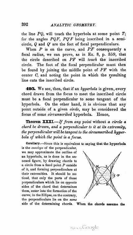
392 ANALYTIC GEOMETRY.
the line PQ, will touch the hyperbola at some point T;
for the angles PQF, PQ'F being inscribed in a semi
circle, Q and Q are the feet of focal perpendiculars.
When P is on the curve, and PF consequently a
focal radius, we can prove, as in Ex. 8, p. 359, that
the circle described on PF will touch the inscribed
circle. The foot of the focal perpendicular must then
be found by joining the middle point of PF with the
center C, and noting the point in which the resulting
line cuts the inscribed circle.
495. We see, then, that if an hyperbola is given, every
chord drawn from the focus to meet the inscribed circle
must be a focal perpendicular to some tangent of the
hyperbola. On the other hand, it is obvious that any
point outside of a given circle, may be considered the
focus of some circumscribed hyperbola. Hence,
Theorem XXXI.—If from any point without a circle a
chord be drawn, and a perpendicular to it at its extremity,
the perpendicular will be tangent to the circumscribed hyper
bola of which the point is a focus.
Corollary.—Since this is equivalent to saying that the hyperbola
is the envelope of the perpendicular,
we may approximate the outline of
an hyperbola, as is done in the an
nexed figure, by drawing chords to
a circle from a fixed point P outside
of it, and forming perpendiculars at
their extremities. It should be no
ticed, that only the parts of these
perpendiculars which lie on opposite
sides of the chord that determines
them, enter into the formation of the
curve; in the Ellipse, on the contrary,
the perpendiculars lie on the same
side of the determining chords. When the chords assume the

NORMAL OF THE HYPERBOLA. 393
limiting positions PL, PR, so as to touch the circle at L and R,
the corresponding perpendiculars LN, MR are the two lines which
we have named the self-conjugates.
496. A little inspection of the equations in Art. 401,
after the sign of b2 has been changed in the first and
second, will show that the reasoning of that article is
entirely applicable to the Hyperbola. Hence,
Theorem XXXII.—The diameters which pass through
the feet of the focal perpendiculars upon any tangent of
an hyperbola, are parallel to the corresponding focal radii
of contact.
Corollary.—Hence, also, as in the case of the Ellipse,
we have the converse theorem, Diameters parallel to the
focal radii of contact meet
the tangent at the feet of its
focalperpendiculars. Con
sequently, after finding the
foot Q of the focal perpen
dicular, we can determine
the point of contact T, if
we wish to do so, by sim
ply drawing F'T parallel to CQ.
It follows, also, that the distance between the foot of the
perpendicular drawn from either focus to a tangent, and
the foot of the perpendicular drawn from the remaining
focus to the parallel tangent, is constant, and equal to the
length of the transverse axis.
THE NORMAL.
497. Equation to the Normal.—From the equa
tion of Art. 402, by changing the sign of b2, we have
a2x b2u
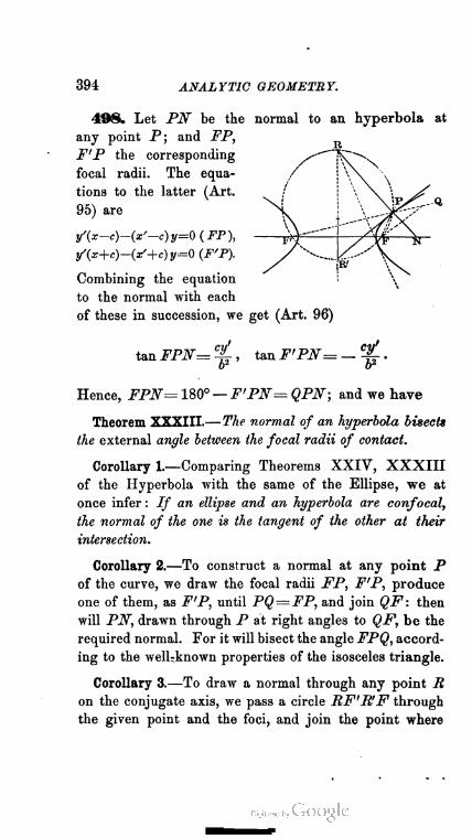
394 ANALYTIC GEOMETRY.
498. Let PN be the normal to an hyperbola at
any point P; and FP,
F'P the corresponding
focal radii. The equa
tions to the latter (Art.
95) are
/(*-<;)-(*'-<:) y=0(.FP),
y'{x+c)-(x'+c)y=Q {F'P).
Combining the equation
to the normal with each
of these in succession, we get (Art. 96)
tan FPN=C-£, twF'PN= — %.
b2 o2
Hence, 2^2^=180°—F'PN=QPN; and we have
Theorem XXXIII.—The normal of an hyperbola bisects
the external angle between the focal radii of contact.
Corollary 1.—Comparing Theorems XXIV, XXXIII
of the Hyperbola with the same of the Ellipse, we at
once infer : If an ellipse and an hyperbola are confocal,
the normal of the one is the tangent of the other at their
intersection.
Corollary 2.—To construct a normal at any point P
of the curve, we draw the focal radii FP, F'P, produce
one of them, as F'P, until PQ=FP, and join QF: then
will PN, drawn through P at right angles to QF, be the
required normal. For it will bisect the angle FPQ, accord
ing to the well-known properties of the isosceles triangle.
Corollary 3.—To draw a normal through any point R
on the conjugate axis, we pass a circle RF'R'F through
the given point and the foci, and join the point where
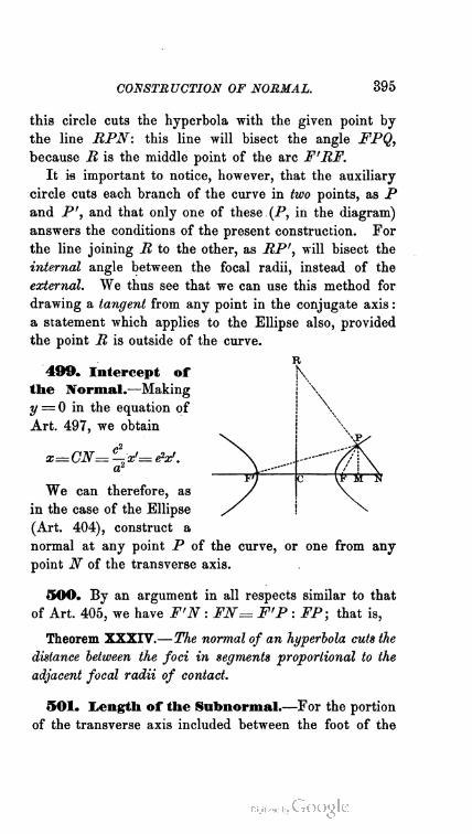
CONSTRUCTION OF NORMAL. 395
this circle cuts the hyperbola with the given point by
the line RPN: this line will bisect the angle FPQ,
because R is the middle point of the arc F'RF.
It is important to notice, however, that the auxiliary
circle cuts each branch of the curve in two points, as P
and P', and that only one of these (P, in the diagram)
answers the conditions of the present construction. For
the line joining R to the other, as MP', will bisect the
internal angle between the focal radii, instead of the
external. We thus see that we can use this method for
drawing a tangent from any point in the conjugate axis :
a statement which applies to the Ellipse also, provided
the point R is outside of the curve.
499. Intercept of
the Normal.—Making
y = 0 in the equation of
Art. 497, we obtain
c2
R
K
x=CN= ■ x'— e2x'.
\
We can therefore, as
in the case of the Ellipse
(Art. 404), construct a
normal at any point P of the curve, or one from any
point iV of the transverse axis.
50O. By an argument in all respects similar to that
of Art. 405, we have F'N : FN= F'P : FP; that is,
Theorem XXXIV.—The normal of an hyperbola cuts the
distance between the foci in segments proportional to the
adjacent focal radii of contact.
501. Length of the Subnormal.—For the portion
of the transverse axis included between the foot of the
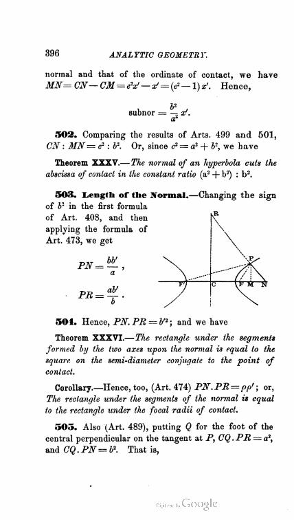
,396 ANALYTIC GEOMETRY.
normal and that of the ordinate of contact, we have
MN= CN— CM=eV— x' = {e2 — 1) x'. Hence,
subnor
502. Comparing the results of Arts. 499 and 501,
CN : MN= <r : b2. Or, since c2 = a2 + b-, we have
Theorem XXXV.—The normal of an hyperbola cuts the
abscissa of contact in the constant ratio (a2 + b2) : b2.
90S. Length of the Normal.—Changing the sign
of b2 in the first formula
of Art. 408, and then
applying the formula of
Art. 473, we get
a
aV
\
\
504. Hence, P~N. PR = b'2 ; and we have
Theorem XXXVI.—The rectangle under the segments
formed by the two axes upon the normal is equal to the
square on the semi-diameter conjugate to the point of
contact.
Corollary.—Hence, too, (Art. 474) PN.PR= pp'; or,
The rectangle under the segments of the normal is equal
to the rectangle under the focal radii of contact.
505. Also (Art. 489), putting Q for the foot of the
central perpendicular on the tangent at P, CQ.PR = a2,
and CQ.PN^b2. That is,

SUPPLEMENTAL CHORDS. 397
Theorem XXXVII.—The rectangle under the normal
and the central perpendicular upon the corresponding
tangent is constant, and equal to the square on the
semi-axis other than the one to which the normal is
measured.
SUPPLEMENTAL AND FOCAL CHORDS.
506. Condition that Chords of an Hyperbola
be Supplemental.—Let
<p, f' denote the inclina
tions of any two supple
mental chords BP, DT.
Then, from Art. 412, by
the characteristic change
of sign, the required condition will be
, b2tan <p tan w'
1 1 a1
507. Hence, the argument of Art. 413 applies directly
to the Hyperbola, and we have
Theorem XXXVIII.—Diameters of an hyperbola which
are parallel to supplemental chords are conjugate.
Corollary 1.— To construct a pair of conjugate diam
eters at a given inclination. The method of solving
this problem in the Hyperbola being identical with
that given for the Ellipse in the first corollary to Art.
413, we do not consider it necessary to repeat the
details here.
Corollary 2.—To construct a tangent parallel to a given
right line. Let LMbe the given line. Draw any diameter
QR, and through its extremity Q pass the chord QS

398 ANALYTIC GEOMETRY.
parallel to LM. Form the supplemental chord SR
and its parallel di
ameter DP: the lat- ..
ter, by the present ^N^/ '
theorem, will be con
jugate to that drawn
parallel to LM; and
(Art. 485) the line
PT, drawn through
its extremity P, and
parallel to LM, will be the tangent required.
Corollary 3.—To construct the axes in the empty curve.
Draw any two parallel chords, bisect them, and form the
corresponding diameter, say QR. On the latter, describe
a semicircle cutting the hyperbola in N. Join RN~, NQ,
and through the middle point of QR draw A'A, B'B par
allel to them : the latter will be the axes, by the same
reasoning as that used in Art. 413, Cor. 3.
308. Focal Chords.—The properties of these chords
presented in Exs. 33—35, p. 361, are as true for the Hy
perbola as for the Ellipse. The reader can easily con
vince himself of this by looking over his solutions of
those examples, and making such changes in the formulae
as the equation to the Hyperbola requires. We shall
here consider only that single property, proved for the
Ellipse in Art. 415, which serves to characterize the
parameter of the curve.
509. For the length of any focal chord in an hyper
bola, we have, by changing the sign of b2 in the formula
at the foot of p. 334,
2 b2
a e2cos2o —1

HYPERBOLA REFERRED TO CONJUGATES. 399
in which d = the inclination of the chord. Hence
(Art. 462), putting a' — the semi-diameter parallel to
the chord,
2a'2 (2a')2cho = = s „ ' ■
a la
That is,
Theorem XXXIX.—Any focal chord of an hyperbola
is a third proportional to the transverse axis and the
diameter parallel to the chord.
Remark.—The latus rectum is the focal chord parallel
to the conjugate axis, and its value (Art. 454, Cor.)
exemplifies this theorem.
ii. The Curve referred to any two Conjugates,
diametral properties.
510. Equation to the Hyperbola, referred to
any two Conjugate Diameters.—The equation to
the primary curve, transformed to two conjugates whose
respective inclinations are 6 and 8', is found hy simply
changing the sign of b2 in the equation at the middle
of p. 336. It is
{a2sm2d— &2cos20) x2 + (a2sin20'— 62cos20') y2=— a2b2.
Hence, by changing the sign of the constant term, the
equation to the conjugate hyperbola, referred to the same
pair of diameters, is
(a2sin20— J2cos20) x2 + (a2sin20' — b2cos2d') y2= a2b\
Now let a', V denote the lengths of the semi-diameters
An. Ge. 37.
400 ANALYTIC GEOMETRY.
of reference : we shall get, by making y — 0 in the first
of these equations, and x = 0 in the second,
a2sin20 — 62cos20 a2sin20'— 62cos20' -- ^ .
a'2 o'1
Substituting in the first equation above, we obtain
*L. _ t..— 1
a'2 6'2 "
Corollary 1.—The transformed equation to the conju
gate curve is therefore
i
a'2 V2
Moreover (since a'2— b'2 = a2 — b2), in the Equilateral
Hyperbola we have b' = a' : hence, the equations to
that curve and its conjugate, referred to any two conju
gate diameters, are
x2—y2=±a'2.
Corollary 2.—The new equation to the Hyperbola
differs from the analogous equation to the Ellipse (Art.
417), only in the sign of V2. Hence, Anyfunction ofb'
that expresses a property of the Ellipse, will be converted
into one expressing a corresponding property of the Hyper
bola by merely replacing its b' by b' V—1.
511. The remarks of Art. 418 evidently apply to the
equations
£ — t — + 1 + i
a2 b2 ' a'2 b'2
Hence, we have the following extensions of Theorems
VI, VII:
DIAMETRAL PROPERTIES. 401
Theorem XL.—The squares on the ordinates to any
diameter of an hyperbola are proportional to the rectangles
under the corresponding segments of the diameter.
Theorem XLI.—The square on any diameter of an hy
perbola is to the square on its conjugate, as the rectangle
under any two segments of the diameter is to the square
on the corresponding ordinate.
512. Writing the equation of Art. 510 in the form
2/2 = ^(*2-«'2),
and comparing it with that of the Equilateral Hyperbola,
namely, with
y2 — x2 — a'2,
we get yh : yr = b' : a'. That is, as the extension of
Theorem VIII,
Theorem XLII.—The ordinate to any diameter of an
hyperbola is to the corresponding ordinate of its equi
lateral, as the conjugate semi-diameter is to the semi-
diameter.
Remark—We may take the corresponding ordinate of the equi
lateral as signifying either the oblique ordinate of the equilateral
described upon the same transverse axis as the given hyperbola, or
the rectangular ordinate of the equilateral described upon the diam
eter selected for the axis of x. For the equation x2 — y1= an will
denote either of these equilaterals, according as it is supposed to
refer to oblique or rectangular axes. Only we must understand
that, in either interpretation, the corresponding ordinates are those
which have a common abscissa.
It is evident, also, that the ratio between the corresponding
ordinates of the hyperbola and the circle x2 + y2 = a'2, described
on any diameter of the curve, is imaginary. Hence, with respect
to this circle, there is a defect in the analogy between the Ellipse

402 ANALYTIC GEOMETRY.
and the Hyperbola: a defect that will be supplied, however, as
soon as we develop the conception of the subtangent to any diameter.
513. We leave the student to show, by interpreting
the equation
bn
that, with reference to any diameter, the Hyperbola
consists of two infinite branches, extending in opposite
directions, and both symmetric to the diameter.
CONJUGATE PROPERTIES OF THE TANGENT.
514. Equation to the Tangent, referred to any
two Conjugate Diameters.—By changing the sign
of bn (Art.. 510, Cor. 2) in the equation of Art. 421,
the equation now sought is seen to be
x'x tfy _
a'2 b'2 '
515. Intercept of the
eter.—Making y — 0 in
the equation just found, we
get, for the intercept in
question,
a'2
x = CT'= ^r.
x
Tangent on any Diam-
Hence, as the extension of Art. 487,
Theorem XLIII.—The intercept cut off by a tangent
upon any diameter of an hyperbola is a third propor
tional to the abscissa of contact and the semi-diameter.
Corollary.—To construct a tangent from any given

INTERCEPTS OF TANGENTS. 403
point. The method of the corollary to Art. 422 applies
directly to the Hyperbola, and the student may interpret
the statements there made, as referring to the present
diagram letter by letter.
516. The properties of tangential intercepts, proved
in Art. 423 with respect to the Ellipse, are also true of
the Hyperbola. We shall
merely restate them here,
leaving the reader to make
such simple modifications of
the analyses in I, II, III
of the article mentioned, as
may be necessary to establish
them. To aid him in this, the parts of the annexed dia
gram are lettered identically with the corresponding parts
of that in Art. 423.
I. Theorem XLIV.-—The rectangle under the intercepts cut off
upon two fixed parallel tangents by any variable tangent of an hyper
bola is constant, and equal to the semi-diameter parallel to the two
tangents.
II. Theorem XLV.—The rectangle under the intercepts cut off
upon any variable tangent of an hyperbola by two fixed parallel
tangents is variable, being equal to the square on the semi-diameter
parallel to the tangent.
III. Theorem XLVI.—The rectangle under the intercepts cut off
upon any variable tangent of an hyperbola by two conjugate diameters
is equal to the square on the semi-diameter parallel to the tangent.
Corollary 1.—By the same reasoning as in the first corollary to
III of Art. 423, we have: Diameters drawn through the intersections
of any tangent with two parallel tangents are conjugate.
Corollary 2.—The problem, Given two conjugate diameters of an
hyperbola in position and magnitude, to construct the axes, is solved
by the same process as the corresponding one on p. 342 ; excepting
that the point P must be taken on the side of D nest to C, instead
of on the side remote from it

404 ANALYTIC GEOMETRY.
517. Subtangent to any Diameter For the
length of this, we have MT'^CM—CT'. Hence,
putting x' — CM, and sub
stituting the value of CT'
from Art. 515,
Xn — an
subtan' - - -. .
x
That is, since vf -f- a'= LM,
and x1 — a' = MB, The sub-
tangent to any diameter of an hyperbola is a fourth pro
portional to the abscissa of contact and the corresponding
segments of the diameter.
Corollary.—If we compare this value of the general
subtangent with that of the subtangent of the curve
(Art. 488), we see at once that the argument used in
Art. 488, Cor. 1, with respect to the Hyperbola and its
inscribed circle, applies to the curve and the circle de
scribed upon any of its diameters. Hence, If through
the head and foot of an ordinate to any diameter of an
hyperbola tangents be drawn to the curve and to the circle
described upon the diameter, they will have d common
subtangent.
In other words, if Q is the point in which a rectangular
ordinate drawn through the foot of a tangent to the hy
perbola pierces the circle mentioned, the tangent to this
circle at Q passes through M, the foot of the ordinate of
contact for the tangent to the hyperbola. The defect
noticed in the Remark under Art. 512, is therefore
supplied; and we may employ the circle in question, to
solve the following problem :
To draw a tangent to an hyperbola from any given point.
Let T' be the given point. Draw the diameter DT'L,
and form the corresponding circle C-DQL. At the given
PARAMETER OF THE HYPERBOLA. 405
point, set up T'Q a rectangular ordinate to this circle,
and through its extremity Q draw the tangent QM.
Then, through the foot M of this tangent, pass MP
parallel to the diameter conjugate to DL : the point P
in which this parallel cuts the hyperbola, will be the
point of contact of the required tangent, which may be
obtained by joining T'P.
Remark.—To form a tangent at any point P of the
curve, we draw the ordinate PM, and, through its foot,
the circular tangent MQ. Then, if QT' be drawn at
right angles to the diameter DL, T' will be the foot
of the required tangent.
518. By the same reasoning as in Art. 425, we get
Theorem XLVII.—The rectangle under the subtangent
and the abscissa of contact is to the square on the ordinate
of contact, as the square on the corresponding diameter is
to the square on its conjugate.
519. Changing the sign of b'2 in the equations of Art.
426, and then taking the steps indicated there, we obtain
Theorem XLVIII.—Tangents at the extremities of any
chord of an hyperbola meet on the diameter which bisects
that chord.
PARAMETERS.
520. Definitions.—The Parameter of an hyperbola,
with respect to any diameter, like the parameter of an
ellipse, is a third proportional to the diameter and its
conjugate. Thus,
(2b')2 2b'2parameter = L_ = ^ .
406 ANALYTIC GEOMETRY.
The parameter with respect to the transverse axis, ia
called the principal parameter; or, the parameter of the
curve. We shall denote its length by 4p.
521. For the value of the parameter of the Hyper
bola, we accordingly have
1 a 262ip= — .c a
Thus (Art. 454, Cor.) the principal parameter is identical
with the latus rectum, and may therefore be described as
the double ordinate to the transverse axis, drawn through
the focus.
522. In Art. 509, we proved that the focal double
ordinate parallel to any diameter is a third proportional
to the transverse axis and the diameter. Now (Art. 463)
the transverse axis is less than any other diameter—less,
therefore, than the diameter conjugate to that of which
the focal chord is a parallel, unless the chord is the latus
rectum. Hence,
Theorem XLIX.—No parameter of an hyperbola, except
the principal, is equal in value to the corresponding focal
double ordinate.
POLE AND POLAR.
523. We now proceed to develop the polar relation
as a property of the Hyperbola ; and shall follow the
steps already twice taken, in connection with the Circle
and the Ellipse.
524. Chord of Contact in the Hyperbola.—Let
x'y' be the fixed point from which the two tangents that
POLAR IN THE HYPERBOLA. 407
determine the chord are drawn. Then, by merely chang
ing the sign of bn in the equation of Art. 431, the equation
to the hyperbolic chord of contact will be
^1 _ tl — 1a'2 bn ~
525. Locos of the Intersection of Tangents to the
Hyperbola.—Let x'y' denote the fixed point through
which the chord of contact belonging to any two of the
intersecting tangents is drawn, and change the sign of
b'2 in the equation of Art. 432 : the equation to the locus
now considered will then be
x'x y'y 1
~o7l ~~ ~V2 = '
526. Tangent and Chord of Contact taken up
into the wider conception of the Polar.—From the
identity in the form of the last two equations with the
form of the equation to the tangent, we see that, in the
Hyperbola also, the law which connects the tangent with
its point of contact, and the chord of contact with the
point from which its determining tangents are drawn, is
the same that connects the locus of the intersection of
tangents drawn at the extremities of chords passing
through a fixed point, with that point.
In short, the three right lines represented by these
equations are only different expressions of the same formal
law : a law, moreover, of which the locus mentioned is the
generic expression. For, in the case of the tangent, the
point x'y' is restricted to being on the curve ; and, in that
of the chord of contact, to being within ; while, in that of
the locus, it is unrestricted : so that the tangent and the
chord of contact are cases of the locus, due to bringing

408 ANALYTIC GEOMETRY.
the point x'y' upon the curve or within it. Moreover, the
formal law which connects the locus with the fixed point
is the law of polar reciprocity. For, by its equation, the
locus is a right line ; and, if we suppose the point x'y' to
be any point on a given right line, the co-efficients of the
equation in Art. 524 will be connected by the relation
Ax1 + By' + C= 0; whence (Art. 117) we have the
twofold theorem:
I. If from a fixed point chords be drawn to any
hyperbola, and tangents to the curve be formed at the
extremities of each chord, the intersections of the several
pairs of tangents will lie on one right line.
II. If from different points lying on one right line
pairs of tangents be drawn to any hyperbola, their several
chords of contact will meet in one point.
The Hyperbola, then, imparts to every point in its
plane the power of determining a right line ; and recip
rocally.
527. Equation to the Polar with respect to an
Hyperbola.—From the conclusions now reached, this
equation, referred to any two conjugate diameters, must
be
5:5 _ t}L — \.a'2 bn~ '
or, referred to the axes of the curve,
x'y' being the point to which the polar corresponds.
52S. Definitions.—The Polar of any point, with re
spect to an hyperbola, is the right line which forms the
locus of the intersection of the two tangents drawn at the
extremities of any chord passing through the point.
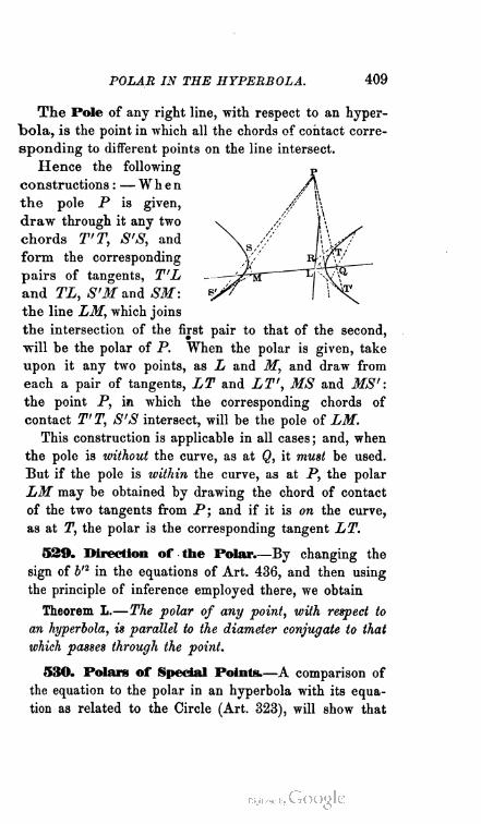
POLAR IN THE HYPERBOLA. 409
The Pole of any right line, with respect to an hyper
bola, is the point in which all the chords of contact corre
sponding to different points on the line intersect.
Hence the following p
constructions : — When f\
the pole P is given,
draw through it any two
chords T'T, S'S, and
form the corresponding
pairs of tangents, T'L
and TL, S'M and SM:
the line LM, which joins
the intersection of the first pair to that of the second,
will be the polar of P. When the polar is given, take
upon it any two points, as L and M, and draw from
each a pair of tangents, LT and LT', MS and MS':
the point P, in which the corresponding chords of
contact T'T, S'S intersect, will be the pole of LM.
This construction is applicable in all cases; and, when
the pole is without the curve, as at Q, it must be used.
But if the pole is within the curve, as at P, the polar
LM may be obtained by drawing the chord of contact
of the two tangents from P; and if it is on the curve,
as at T, the polar is the corresponding tangent LT.
529. Direction of the Polar.—By changing the
sign of b'2 in the equations of Art. 436, and then using
the principle of inference employed there, we obtain
Theorem L.—The polar of any point, with respect to
an hyperbola, is parallel to the diameter conjugate to thai
which passes through the point.
530. Polars of Special Points.—A comparison of
the equation to the polar in an hyperbola with its equa
tion as related to the Circle (Art. 323), will show that

410 ANALYTIC GEOMETRY.
the general properties proved of polars in Art. 324 are
true for the Hyperbola. We therefore pass at once to
those special properties which characterize the polars of
certain particular points.
Applying the processes of Art. 437 to the equation of
Art. 527, we get
I. The polar of the center is a right line at infinity.
II. The polar of any point on a diameter is a right
line parallel to the conjugate diameter, and its distance
from the center is a third proportional to the distance of
the point and the length of the semi-diameter.
III. The polar of any point on the transverse axis is
the perpendicular whose distance from the center is a
third proportional to the distance of the point and the
length of the semi-axis.
Corollary.—From II it follows, that the construction
for the polar, given under Art. 437 with respect to the
Ellipse, is entirely applicable to the Hyperbola.
531. Polar of the Focus.—The equation to this is
found by putting (± ae, 0) for x'y' in the second equa
tion of Art. 527, and is therefore
Hence, The polar of either focus in an hyperbola is the
perpendicular which cuts the transverse axis at a distance
from the center equal to a : e, measured on the same side
as the focus.
Remark.—Since the e of the Hyperbola is greater than
unity, the distance of the focal polar from the center is
in that curve less than a. In the Ellipse, on the contrary,
this distance is greater than a, because the e of that curve
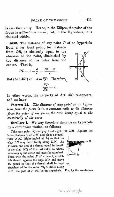
POLAR OF THE FOCUS. 411
is less than unity. Hence, in the Ellipse, the polar of the
focus is without the curve ; but, in the Hyperbola, it is
situated within:
532. The distance of any point P of an hyperbola
from either focal polar, for instance
from DR, is obviously equal to the
abscissa of the point, diminished by
the distance of the polar from the
center. That is,
a ex — a
e
But (Art. 457) ex— a =FP. Therefore,
Fp_PD~e-
In other words, the property of Art. 439 re-appears,
and we have
Theorem LI.—The distance of any point on an hyper
bola from the focus is in a constant ratio to its distance
from the polar of the focus, the ratio being equal to the
eccentricity of the curve.
Corollary 1.—We may therefore describe an hyperbola
by a continuous motion, as follows :
Take any point F, and any fixed right line DR. Against the
latter, fasten a ruler DLV, and place a second
ruler NQL (right-angled at L) so that its
edge LN may move freely along DD'. At
F fasten one end of a thread equal in length
to the edge NQ of this last ruler, to whose
extremity Q the other end must he attached.
Then, with the point P of a pencil, stretch
this thread against the edge NQ, and move
the pencil so that the thread shall he kept jyl
stretched while the ruler NQL slides along
DD': the path of P will be an hyperbola. For, by the conditions
412 ANALYTIC GEOMETRY.
named, FP must equal PN in every position of the pencil : whence
FP : PD = NQ : QL. That is, since DR must be the polar of
F with respect to some hyperbola, the focal distance of P is in a
constant ratio to its distance from the focal polar.
This construction derives interest from a comparison
with that of the Ellipse in Art. 439, Cor. 1. It will be
seen that the essential principle is the same in both,
namely, the use of the parts of a right triangle to de
termine a constant ratio between the distances of points
from a fixed point and a fixed right line. It is notice
able, that, in the Ellipse, this constant ratio is that of
the base to the hypotenuse ; while, in the Hyperbola, it
is that of the hypotenuse to the base; thus illustrating
the inverse relation existing between the two curves.
Corollary 2.—In the construction just explained, the
polar of the focus is used as the directing line of the
motion which generates the curve. For this reason, it
is called the directrix of the corresponding hyperbola.
Corollary 3.—In the light of the present theorem, we
may interpret the name hyperbola as denoting the conic
in which the constant ratio between the focal and polar
distances exceeds unity.
533. Focal Angle subtended by any Tangent.—By exam
ining the investigation conducted in Art. 440, the student will see
that it is applicable to the Hyperbola, with the single exception of
a change in the sign of the final result. Hence, if p — the focal
distance of any given point from which a tangent is drawn to an
hyperbola, and x = the abscissa of the point, the angle <? which the
portion of the tangent intercepted between the given point and the
point of contact subtends at the focus, will be determined by the
formula
ex — acos <j> = •
P
534. This expression, being independent of the point of con
tact #y, would seem to indicate that both of the tangents that can

HYPERBOLA REFERRED TO ITS FOCI. 413
be drawn from a given point to the curve subtend the same focal
angle. It is found, however, as in the case presented in the dia
gram, that when the given point P is taken under such conditions
(Art. 484, Cor. 2) as fix the two
points of contact T and T' on \ ^
opposite branches of the curve, N>i' 7^
the angles PFT, PFT' are not y^^7—^-.^/^
equal, but supplemental. But, J \
whether they be the one or the / \ /\.
other, the line FP must bisect j> \
the whole angle T'FT subtended
by the chord of contact, either internally or externally. Hence,
Theorem LII.—The right line that joins the focus io the pole of any
chord, bisects the focal angle which the chord subtends.
Corollary.—The angle subtended by a focal chord being 180°,
we have, as a special case of the preceding: The line that joins
the focus to the pole of any focal chord is perpendicular to the chord.
in. The Curve referred to its Foci.
535. In the polar equations of Art. 172 and the
subjoined Remark, namely, in
qfl-e*) a(e>-l)
" 1 — e cos 0 ' 1 — ecosfl'
we now know that the constant a is the transverse semi-
axis of the corresponding hyperbola, and the constant e
its eccentricity.
Replacing, then, e2 — 1 by its value (Art. 171) b2:a?,
we may write these equations
b2 1 b2 1
r a 1 — ecosd' a 1 — e cos 6
But (Art. 521) b2 : a is half the parameter of the curve.
± 2»
1 — e cos a
414 ANALYTIC GEOMETRY.
1
the upper sign corresponding to the right-hand focus,
and the lower to the left-hand.
538. Polar Equation to the Tangent.—By an
analysis exactly similar to that in Art. 444, we find this
to be
a(l— e2)
P ~ cos (p — 0')—e cos 0 '
Corollary.—The equation to the diameter conjugate to
x'i/ (Art. 469) differs from that of the tangent at s/y'
only in having 0 for its constant term. Hence, as in
the corollary to Art. 444,
ae (cos 6'— e)
'" = cos (V — 0') — ecos ~d
is the polar equation to the diameter conjugate to that
which passes through p'O'.
iv. The Cueve referred to its Asymptotes.
j 537. Hitherto, the properties established for the
Hyperbola have had a fixed relation, either of identity
or of antithesis, to those of the Ellipse. We now come,
however, to a series of properties peculiar to the Hyper
bola, arising from the presence of the two lines which
we have named the self-conjugate diameters. We might
proceed at once to transform the equation of Art. 167
to these diameters as axes of reference ; but, before
doing so, let us subject the self-conjugates themselves
o a more minute examination.
"*-S. Definition.—An Asymptote of any curve is a
nich continually approaches the curve, but meets
nly at infinity.

ASYMPTOTES OF THE HYPERBOLA. 415
Asymptotes are either curvilinear or rectilinear. The
term asymptote is derived from the Greek a privative,
and ouuxixzscv, to coincide, and may be taken as signi
fying that the line to which it is applied never meets the
curve which it forever approaches.
539. We have already once or twice spoken of the
self-conjugates of the Hyperbola as its asymptotes. We
now proceed to show that they are such. We have
proved (Arts. 461, Cor. 1 ; 480) that they meet the
curve only at infinity : it remains to show that they
draw nearer and nearer to the curve the farther they
recede from the center.
Let CM be any common abscissa of an hyperbola and
its self-conjugate diameter CL. The equations to CL
and the curve being respectively
y=-x, y-
■ \/x- -
we get, for the difference between
any two corresponding ordinates, B'
PQ=h- (x-V/^=^)= f-
Hence, as x increases, PQ diminishes ; so that, if we
suppose x to be increased without limit, or the point P
of the curve to recede to an infinite distance from the
origin, PQ will converge to the limit 0. Now the
distance of any point P of the curve from the self-
conjugate CL is equal to PQ sin PQC : therefore, as
the angle PQC is the same for every position of P,
this distance diminishes continually as P recedes from
the center; or, we have
An. Ge. 38.

416 ANALYTIC GEOMETRY.
Theorem LIII.—The self-conjugate diameters of an
hyperbola are asymptotes of the curve.
Remark.—We have inferred this theorem with respect to L'R
as well as LR', although the preceding investigation is conducted
in terms of LR' only. But it is manifest that a similar analysis
applies to L'R; and it can be shown, in like manner, that LR'
and L'R are asymptotes of the conjugate hyperbola. We leave the
proof of this, however, as an exercise for the student
540. Angle between the Asymptotes.—From Art.
479, we have tan LCM=b : a, and tanL'CM=— b : a;
hence LCM= 180° —L'CM= ROM. If, then, we put
(p = the required angle LOR, and 0 = LCM, we shall
get <p = 2d ; or, since tan 6~b: a, and therefore cos d =
a : c,
(p = 2 sec-1 e.
Hence, if the eccentricity of an hyperbola is given,
the inclination of its asymptotes is also given ; for it is
double the angle whose secant is the eccentricity. Con
versely, when the inclination of the asymptotes is known,
the eccentricity is found by taking the secant of half the
inclination.
Thus, in the case of an equilateral hyperbola, whose
eccentricity (Art. 456, Cor.) = j/2, we have
^ = 2sec-'l/2=90°:
which agrees with the property by which (Art. 177, Cor.)
we originally distinguished this curve.
541. Equations to the Asymptotes.—These are
respectively (Art. 479) y = (b : a) x, y = — (b : a) x.
Or we may write them
a b a b
\
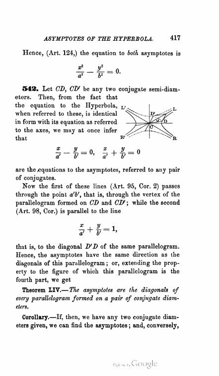
ASYMPTOTES OF THE HYPERBOLA. 417
Hence, (Art. 124,) the equation to both asymptotes is
± - t- = 0.
a' ¥
542. Let CD, CD' be any two conjugate semi-diam
eters. Then, from the fact that
the equation to the Hyperbola,
when referred to these, is identical
in form with its equation as referred
to the axes, we may at once infer
that
a' b' ~ a' + b'
are the /equations to the asymptotes, referred to any pair
of conjugates.
Now the first of these lines (Art. 95, Cor. 2) passes
through the point a'b', that is, through the vertex of the
parallelogram formed on CD and CD'; while the second
(Art. 98, Cor.) is parallel to the line
„i ^ V '
that is, to the diagonal D'D of the same parallelogram.
Hence, the asymptotes have the same direction as the
diagonals of this parallelogram ; or, extending the prop
erty to the figure of which this parallelogram is the
fourth part, we get
Theorem LIV.—The asymptotes are the diagonals of
every parallelogram formed on a pair of conjugate diam
eters.
Corollary.—If, then, we have any two conjugate diam
eters given, we can find the asymptotes ; and, conversely,

418 ANALYTIC GEOMETRY.
given the asymptotes and any diameter CD, we can find
its conjugate by drawing DO parallel to CM, and pro
ducing it till OD' = OD, when D1 will be the extremity
of the conjugate sought.
543. From the equation to the tangent (Art. 481)
we get
_ JVx _ 6* .
V ~ ay y' '
or, after substituting for y' from
the equation to the curve, and
factoring,
b 1 _ b*
■ ;;! •'"
Supposing, then, that x' and y' are increased without
limit, or that the point of contact P recedes to an infinite
distance from the origin, the limiting form to which this
equation tends is
b
y ~ — x.
But this (Art. 541) is the equation to CL; and a like
result can be readily obtained with respect to the other
asymptote. Hence,
Theorem LV.— The asymptotes are the limits to which
the tangents of an hyperbola converge as the point of
contact recedes toward infinity.
Remark—We might therefore define the asymptotes as the right
lines which meet the hyperbola in two consecutive points at infinity.
544. Accordingly, by Theorem XXIX (Art. 493), the
product of the focal perpendiculars upon an asymptote

ASYMPTOTES OF THE HYPERBOLA. 419
must be equal to b2. But, since the asymptote passes
through the center, these focal perpendiculars must be
equal to each other, and therefore each equal to b.
That is,
Theorem LVI.—The perpendicular from either focus to
an asymptote is equal to the conjugate semi-axis.
545. Let FP be the focal dis
tance of any point on an hyperbola,
and PD its distance from the direc
trix DB. By Art. 532, FP=e.PD.
But (Art. 540), e= sec LGF. Hence,
FP=PD secLCF=PB cosec PRD,
if PR be drawn parallel to the asymp
tote CL. That is (Trig., 859), FP =
PR; or, we have
Theorem LVII.—The focal distance of any point on an
hyperbola is equal to its distance from the adjacent direc
trix, measured on a parallel to either asymptote.
Corollary—We here find a new reason
for the method of generating an hyperbola,
given in the first corollary to Art. 532.
For, by the requirements of the method,
FP= PB = e.PD. Now, by the diagram,
PR = PD sec RPD. Hence, the method
makes sec RPD — e\ that is (Art. 540), it
makes the angle RPD equal to the inclina
tion of the asymptote, and PR therefore par
allel to that line.
546. Equation to the Hyperbola, referred to its
Asymptotes.—The equation to the Hyperbola, trans
formed to a pair of oblique axes whose inclinations to
the transverse axis are respectively 0 and 6', is found

420 ANALYTIC GEOMETRY.
by changing the sign of b2 in the first equation of p. 336,
and is
(a2 sin2 0 — b2 cos2 0) x2 + (a2 sin2 0' — b2 cos2 0') ?/2
+ 2 (a2 sin 0 sin 0' — b2 cos 0 cos 0') =—- a262.
If, then, the new axes are the asymptotes, and there
fore (Art. 479) tan2 0 = b2 : a2 = tan2 0', we shall have
a2 sin2 0 — b2 cos2 0 = 0 = a2 sin2 0' — 62 cos2 0' ; and the
equation will become
2 (a2 sin 0 sin 0'— 62 cos 0 cos 0') zy =— a2b2.
In this, again, since* sin0 = — b : Va2 + 62 =— sin 0',
and cos 0 — a : Va2 + 62 = cos 0', it is evident that we
have a2 sin 0 sin 0' — 62 cos 0 cos 0' = — 2 a2*2 : (a2 + b2).
Hence, the required equation is
a2+ b2
and putting k2 to represent the constant in the second
member, we may write it in the form in which it is
usually quoted, namely,
xy = k2.
Corollary.—Hence, the equation to the conjugate hy
perbola will be
xy = — k2;
and, in the case of an equilateral hyperbola, we shall
have
* It must be remembered that 0 = the inclination of the new axis of x;
and, in our investigation, the axis of x is that asymptote which corre
sponds to 8 = tan-1 — b : a.
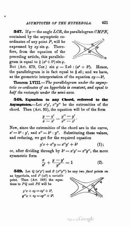
ASYMPTOTES OF THE HYPERBOLA. 421
547. If ip — the angle LGR, the parallelogram CMPN,
contained by the asymptotic co
ordinates of any point P, will be
expressed by xy sin <p. There
fore, from the equation of the
preceding article, this parallelo
gram is equal to 5 (a2 + b2) sin <p.
But (Art. 479, Cor.) sin <p = 2ab : (a2 + b2). Hence,
the parallelogram is in fact equal to \ ab ; and we have,
as the geometric interpretation of the equation xy= k2,
Theorem LVIII.—The parallelogram under the asymp
totic co-ordinates of an hyperbola is constant, and equal to
half the rectangle under the semi-axes.
548. Equation to any Chord, referred to the
Asymptotes.—Let x'y', x"y" be the extremities of the
chord. Then (Art. 95), the equation will be of the form
y — ¥
x"
Now, since the extremities of the chord are in the curve,
x' =k2 : y', and x" = k2 : y". Substituting these values,
and reducing, we get for the required equation
y'x + x"y = x"y' + k2 (1) ;
or, after dividing through by k2 = x'y' = x"y", the more
symmetric form
1 (2).— _l y — y'
2/ ^ y"
549. Let Q {x'y') and S (x"y") be any two fixed points on
an hyperbola, and P (aff) a variable
point. Then (Art. 548) the equa
tions to PQ and PS will be
y'x + ay = ay/ +
y"x + ay = ay" +lc\

422 ANALYTIC GEOMETRY.
Making y = 0 in each of these, we get CM= a-\- 3/, CT= a + x".
Hence, MT=x" — x\ which being independent of a/3, we have
Theorem LIX.—The right lines which join two fixed points of an
hyperbola to any variable point on the curve, include a constant portion
of the asymptote.
550. Equation to the Tangent, referred to the
Asymptotes.—Assuming that the point x"y" in the final
equation of Art. 548 becomes coincident with x'y', we
get, for the equation now sought,
x
551. Equations to Diameters, referred to the
Asymptotes.—The diameter which passes through a
fixed point x'y' (Art. 95, Cor. 2), is represented by
y'x — x'y — 0 ; and this equation, when x'y' is on the
curve, may be written (Art. 546)
» _ 3L = 0 (l).k* y'1 y '
The equation to the diameter conjugate to x'y' must
have 0 for its absolute term (Art. 63) ; and, as the
diameter is parallel to the tangent at x'y1, the variable
part of its equation (Art. 98, Cor.) must be identical
with that of the tangent. Hence, the equation is
^ + y-,= 0 (2).
x> y'
The transverse axis bisects the angle between the
asymptotes, and therefore, at its extremity, x1 = y'.
Hence, the equations to the axes, referred to the
asymptotes, are
x — y = 0, x + y = 0 (3).

ASYMPTOTES OF THE HYPERBOLA. 423
552. Eliminating between (2) of the preceding article,
and the equation to the conjugate hyperbola, we get, for
the co-ordinates of the extremity of the diameter conju
gate to x'y',
*c = =F z', yc = ± y'.
553. From the equation
to the tangent (Art. 550),
we get, by making y and x
successively equal to zero,
CT = 2x', and OS = 2y'.
Hence, P is the middle point
of ST; and we have
Theorem LX.—The portion of the tangent included
between the asymptotes, is bisected at the point of
contact.
Corollary.—Since (Art. 542) S is a vertex of the par
allelogram formed on the conjugate semi-diameters CP
and CD, we have PS=CD. Hence, ST=2PS=Diy.
That is, The segment cut from the tangent by the asymp
totes is equal to the diameter conjugate to the point of
contact.
Remark.—Theorem LX might have been obtained geometrically,
as a corollary to Theorem L1V.
554. From the preceding article, we at once obtain
CT. CS=\x'y' = a2 + i2,
since 4 x'y' = 4k2. That is,
Theorem LXI.—The rectangle under the intercepts cut
off upon the asymptotes by any tangent is constant, and
equal to the sum of the squares on the semi-axes.
An. Ge. 39

424 ANALYTIC GEOMETRY.
555. For the area of the triangle SOT, we have
T=2 x'y' sin <p = ah,
since 2 x'y' = 2F, and sin^> = 2a£> : (a2-\-b2). Hence,
Theorem LXII.—The triangle included between any
tangent and the asymptotes is constant, and equal to the
rectangle under the semi-axes.
556. The equations to the tangents at the extremi
ties of two conjugate diameters (Arts. 550, 552) are
- 4. y- — 2 x- _ 2
x' ^ y'~ ' x> y'~
Adding these together, we get x — 0, the equation to
the line CL. Hence,
Theorem LXIII.—Tangents at the extremities of conju
gate diameters meet on the asymptotes.
557. The equation to Q'Q, an ordinate to any diam
eter VD, will only differ
from that of the conjugate
diameter VD1 by some con
stant, which we may call 2c.
The equation will therefore
[Art. 551, (2)] be
x1 + y>
= 2c.
Now this, when combined with the equation to VD,
x1 y'~V>
gives x = cxf, y = cy' as the co-ordinates of M, the point
in which Q'Q cuts VD. But the intercepts' of Q'Q upon
the asymptotes are obviously CQ' = 2cxf, CQ = 2cy''.
Hence, M is the middle point of Q'Q; or, we have
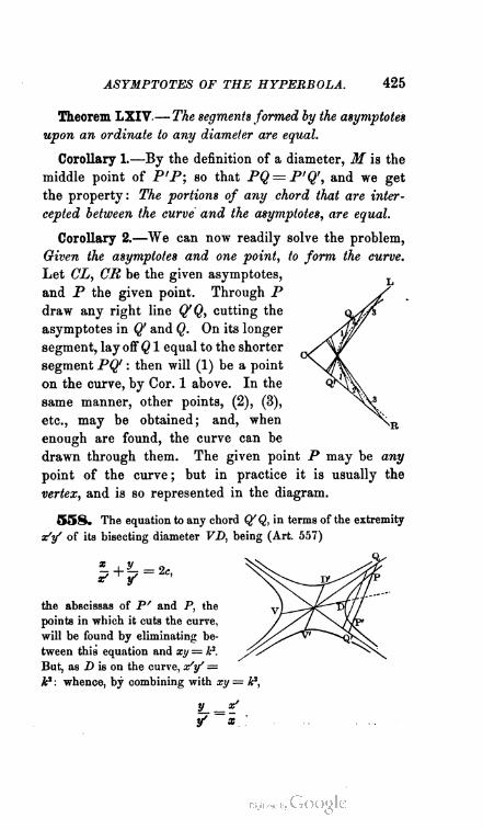
ASYMPTOTES OF THE HYPERBOLA. 425
Theorem LXIV.—The segments formed by the asymptotes
upon an ordinate to any diameter are equal.
Corollary 1.—By the definition of a diameter, M is the
middle point of P'P; so that PQ — P'Q', and we get
the property: The portions of any chord that are inter
cepted between the curve and the asymptotes, are equal.
Corollary 2.—We can now readily solve the problem,
Given the asymptotes and one point, to form the curve.
Let CL, CR be the given asymptotes,
and P the given point. Through P
draw any right line Q'Q, cutting the
asymptotes in Q' and Q. On its longer
segment, lay off Q 1 equal to the shorter
segment PQ' : then will (1) be a point
on the curve, by Cor. 1 above. In the
same manner, other points, (2), (3),
etc., may be obtained; and, when
enough are found, the curve can be
drawn through them. The given point P may be any
point of the curve ; but in practice it is usually the
vertex, and is so represented in the diagram.
558. The equation to any chord Of Q, in terms of the extremity
x'y' of its bisecting diameter VD, being (Art. 557)
= 2C,
the abscissas of P' and P, the
points in which it cuts the curve,
will be found by eliminating be
tween this equation and xy= k'.
But, as D is on the curve, x'y' =
A* : whence, by combining with xy = k*,
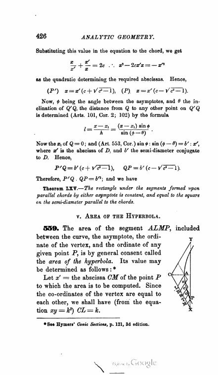
426 ANALYTIC GEOMETRY.
Substituting this value in the equation to the chord, we get
% + — = 2c .-. x1 — 2cx/x = — x"1
as the quadratic determining the required abscissas. Hence,
(P') x = x'(c + YcT=~l), (P). x = x'(c—Vl?=~l).
Now, <p being the angle between the asymptotes, and 6 the in
clination of Of Q, the distance from Q to any other point on 0/Q
is determined (Arts. 101, Cor. 2; 102) by the formula
^ x— Xi (x — Xi) sin (j>
~~ h sin — 0)
Now the Xi of Q = 0 ; and (Art. 553, Cor. ) sin <j> : sin (</> — ") = b' : x/,
where x' is the abscissa of D, and 1/ the semi-diameter conjugate
to D. Hence,
P'Q= 6'(C+ t/?=1), QP = A/(c-V/?^r"l).
Therefore, P'Q . QP=i/2; and we have
Theorem LXV.—The rectangle under the segments formed upon
parallel chords by either asymptote is constant, and equal to the square
on the semi-diameter parallel to the chords.
v. Area op the Hyperbola.
559. The area of the segment ALMP, included
between the curve, the asymptote, the ordi
nate of the vertex, and the ordinate of any
given point P, is by general consent called
the area of the hyperbola. Its value may
be determined as follows : *
Let x' = the abscissa CM of the point P
to which the area is to be computed. Since
the co-ordinates of the vertex are equal to
each other, we shall have (from the equa
tion xy — A2) CL — k.
* See Hymers' Conic Sections, p. 121, 3d edition.
\

AREA OF THE HYPERBOLA. 427
It is customary to take the quantity k as the unit in
this computation. Adopting this convention, let the
distance LMbe so subdivided at n points R, S, . . . , M,
that the abscissas CL, CR, CS, . . . , CM may increase
by geometric progression. Then, if CR= x, we shall have
CL= 1, CR = x, CS = x*, . . . , C3f=x".
Thus x? = x" ; or, x = 2/" : so that, as n increases, x
diminishes, and converges toward 1 as n converges to
infinity. Now, at R, S, . . . , M, erect n ordinates, and
form n corresponding parallelograms RA, Sa, . . . , Mb,
situated as in the figure. Then
area RA = RL . LA sin <f> = ( CR — CL) LA sin p = (x — 1 ) sin <j>,
" Sa = SR . Ra sin <j> = (x1 — x) — sin <p = (a: — 1 ) sinx
" Te=TS.Se sin (x3 — r1) ^ sin <S> = (x — 1 ) sin 0,
and so on for the whole series of n parallelograms.
Hence, replacing x by its value a/« , and putting I =
the sum of the n parallelograms, we get
1
I = n (x' » — 1) sin cp.
But an inspection of the diagram shows that the
greater the number of the parallelograms, the more
nearly does the sum of their areas approach the area
ALMP. And since x, the ratio of the successive
abscissas, tends to 1 as n tends to 00, we can make the
number of the equal parallelograms as great as we
please ; in other words, the true value of the area
ALMP is the limit toward which 2' converges as n
converges to co. Hence,
\_ 2area ALMP = n {x'n — 1 ) sin <p = n [j 1 + {3/— 1) }n — 1] sin 9

428 ANALYTIC GEOMETRY.
Now [Alg., 373, (5)] the series in the braces denotes the
Naperian logarithm of x'. Therefore, calling this loga
rithm lx', and the hyperbolic area A, we obtain
A — sin <p . lx'.
But (Alg., 376) sin <p . I x' = the logarithm of x' in a
system whose modulus = sin f. Hence,
Theorem LXVI.—The area of any hyperbolic segment
is equal to the logarithm of the abscissa of its extreme point,
taken in a system whose modulus is equal to the sine of the
angle between the asymptotes.
Corollary.—In an equilateral hyperbola, since <p = 90°,
sin <p — 1 ; and we get A = lx'. That is, The area of an
equilateral hyperbola is equal to the Naperian logarithm
of the abscissa of the extreme point.
For this reason, Naperian logarithms are called hyper
bolic. But, as we have just seen, the title belongs with
equal propriety to logarithms with any modulus.
EXAMPLES ON THE HYPERBOLA.
1. Prove that the middle points of a series of parallels inter
cepted between an hyperbola and its conjugate, lie on the curve
2 Find the several loci of the centers of the circles inscribed
and escribed to the triangle F'PF, F' and F being the foci of any
hyperbola, and P any point on the curve.
EXAMPLES ON THE HYPERBOLA. 429
3. An ellipse and a pair of conjugate hyperbolas are described
upon the same axes, and, at the points where any line through the
center meets the ellipse and one of the hyperbolas, tangents are
drawn : find the locus of their intersection.
4. In any triangle inscribed in an equilateral hyperbola, the
three perpendiculars from the vertices to the sides, converge in a
point upon the curve.
5. To determine the hyperbola which has two given lines for
asymptotes, and passes through a given point.
6. Between the sides of a given angle, a right line moves so as
to inclose a triangle of constant area: the locus of the center of
gravity in the triangle is the hyperbola represented by
9 xy Bin 4> = 2k*,
where <? = the given angle, and k* = the constant area.
7. QQf is a double ordinate to the axis major A'A of an ellipse ;
QA, A'Qf are produced to meet in P: find the locus of P.
8. To a series of con focal ellipses, tangents are drawn having a
constant inclination to the axes : the locus of the points of contact
is an hyperbola concentric with the ellipses.
9. The radius of the circle which touches an hyperbola and its
asymptotes, is equal to that part of the latus rectum produced
which is intercepted between the asymptote and the curve.
10. About the focus of an hyperbola, a circle is described with
a radius equal to the conjugate semi-axis, and tangents are drawn
to it from any point on the curve : their chord of contact is tangent
to the inscribed circle.
1 1 . Tangents to an hyperbola are drawn from any point on either
branch of the conjugate curve: their chord of contact touches the
opposite branch.
12. In any equilateral hyperbola, let d = the inclination of a
diameter passing through any point P, and = that of the polar
of P, the transverse axis being the axis of x : then will
tan if tan = 1.
13. The circle which passes through the center of an equilateral
hyperbola and any two points A and B, passes also through the
intersection of two lines drawn the one through A parallel to the
polar of B, and the other through B parallel to the polar of A.
430 ANALYTIC GEOMETRY.
14. The locus of a point such that the rectangle under the focal
perpendiculars upon its polar with respect to a given ellipse shall
be constant, is an ellipse or an hyperbola according as the foci are
on the same side or on opposite sides of the polar.
15. A line is drawn at right angles to the transverse axis of aii
hyperbola, meeting the curve and its conjugate in P and Q: show
that the normals at P and Q intersect upon the transverse axis.
Also, that the tangents at P and Q intersect on the curve
4 \ul a' i ~ a'
16. Given two unequal circles: the locus of the center of the
circle which touches them both externally, is an hyperbola whose
foci are the centers of the given circles.
17. Every chord of an hyperbola bisects the portion of either
asymptote included between the tangents at its extremities.
18. If a pair of conjugate diameters of an ellipse be the asymp
totes of an hyperbola, to prove that the points of the hyperbola at
which its tangents will also touch the ellipse, lie on an ellipse con
centric and of the same eccentricity with the given one.
19. A tangent is drawn at a point P of an hyperbola, cutting
the asymptote CY in E; from E is drawn any right line EKH
cutting one branch of the curve in A* H; and Kk, PM, Hh are
drawn parallel to CY cutting the asymptote CK in h, M, h: to
prove that
Ilh + Kk = IMP.
20. Three hyperbolas have parallel asymptotes: show that the
three right lines which join two and two the intersections of the
hyperbolas, meet in one point
CHAPTER FIFTH.
THE PARABOLA.
i. Tiie Curve referred to its Axis and Vertex.
560. In discussing the Parabola, we shall find it
most convenient to transform its equation, as found in
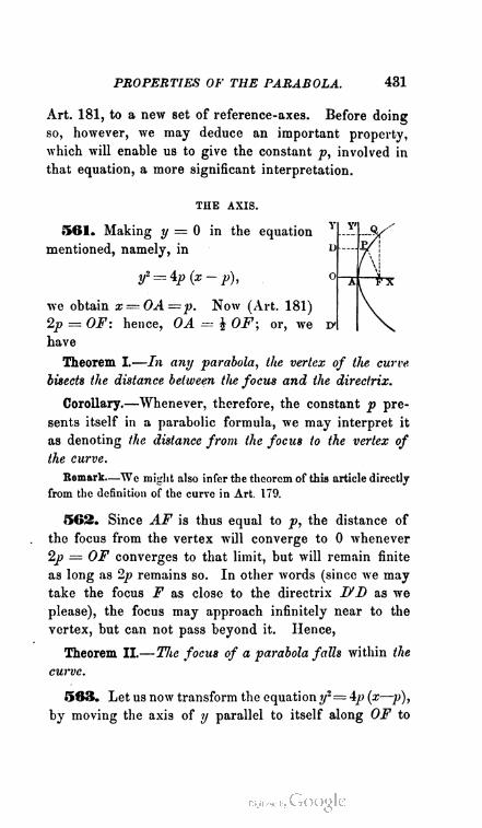
PROPERTIES OF THE PARABOLA. 431
Art. 181, to a new set of reference-axes. Before doing
so, however, we may deduce an important property,
which will enable us to give the constant p, involved in
that equation, a more significant interpretation.
THE AXIS.
561. Making y — 0 in the equation
mentioned, namely, in
y2=--4p(x- p),
we obtain x = OA =p. Now (Art. 181)
2p = 0F: hence, OA = & OF; or, we
have
Theorem I.—In any parabola, the vertex of the curve
bisects the distance between the focus and the directrix.
Corollary.—Whenever, therefore, the constant p pre
sents itself in a parabolic formula, we may interpret it
as denoting the distance from the focus to the vertex of
the curve.
Remark—Wc might also infer the theorem of this article directly
from the definition of the curve in Art. 179.
562. Since AF is thus equal to p, the distance of
the focus from the vertex will converge to 0 whenever
2p = OF converges to that limit, but will remain finite
as long as 2p remains so. In other words (since we may
take the focus F as close to the directrix D'D as we
please), the focus may approach infinitely near to the
vertex, but can not pass beyond it. Hence,
Theorem II.—The focus of a parabola falls within the
curve.
*563. Let us now transform the equation y*—4p (x—p),
by moving the axis of y parallel to itself along OF to
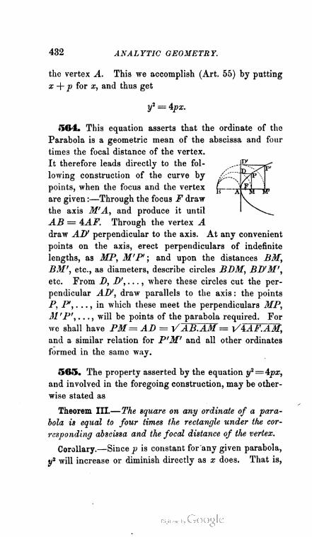
432 ANALYTIC GEOMETRY.
the vertex A. This we accomplish (Art. 55) by putting
x + p for x, and thus get
y2 — 4px.
564. This equation asserts that the ordinate of the
Parabola is a geometric mean of the abscissa and four
times the focal distance of the vertex.
It therefore leads directly to the fol
lowing construction of the curve by
points, when the focus and the vertex
are given :—Through the focus F draw
the axis M'A, and produce it until
AB — 4AF. Through the vertex A
draw AD' perpendicular to the axis. At any convenient
points on the axis, erect perpendiculars of indefinite
lengths, as MP, M'P'; and upon the distances BM,
BM', etc., as diameters, describe circles BBM, BD'M',
etc. From B, B', . . . , where these circles cut the per
pendicular AB', draw parallels to the axis : the points
P, P1, . . . , in which these meet the perpendiculars MP,
M 'P', . . . , will be points of the parabola required. For
we shall have PM= AB = VAB.AM= ViAF.A~M,
and a similar relation for P'M' and all other ordinates
formed in the same way.
565. The property asserted by the equation y2— 4px,
and involved in the foregoing construction, may be other
wise stated as
Theorem III.—The square on any ordinate of a para
bola is equal to four times the rectangle under the cor
responding abscissa and the focal distance of the vertex.
Corollary.—Since p is constant for any given parabola,
y2 will increase or diminish directly as x does. That is,
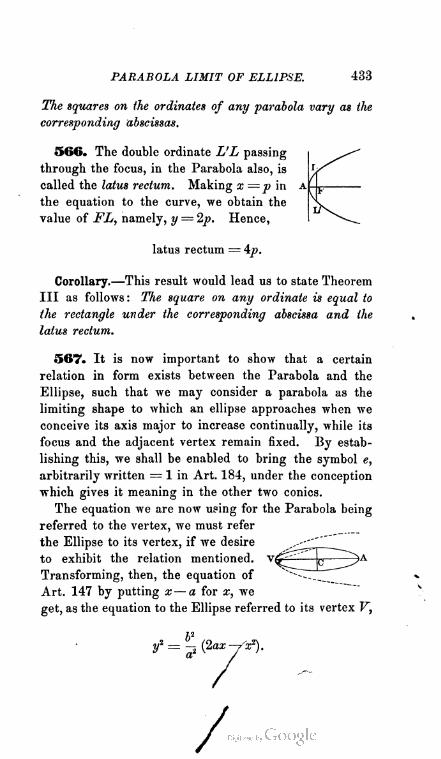
PARABOLA LIMIT OF ELLIPSE. 433
The squares on the ordinates of any parabola vary as the
corresponding abscissas.
566. The double ordinate L'L passing
through the focus, in the Parabola also, is
called the latus rectum. Making x —p in
the equation to the curve, we obtain the
value of FL, namely, y = 2p. Hence,
latus rectum = \p.
Corollary.—This result would lead us to state Theorem
III as follows: The square on any ordinate is equal to
the rectangle under the corresponding abscissa and the
latus rectum.
567. It is now important to show that a certain
relation in form exists between the Parabola and the
Ellipse, such that we may consider a parabola as the
limiting shape to which an ellipse approaches when we
conceive its axis major to increase continually, while its
focus and the adjacent vertex remain fixed. By estab
lishing this, we shall be enabled to bring the symbol e,
arbitrarily written = 1 in Art. 184, under the conception
which gives it meaning in the other two conies.
The equation we are now using for the Parabola being
referred to the vertex, we must refer
the Ellipse to its vertex, if we desire
to exhibit the relation mentioned.
Transforming, then, the equation of
Art. 147 by putting x— a for x, we
get, as the equation to the Ellipse referred to its vertex V,
b2y* = -t (Zaxyx*).
/
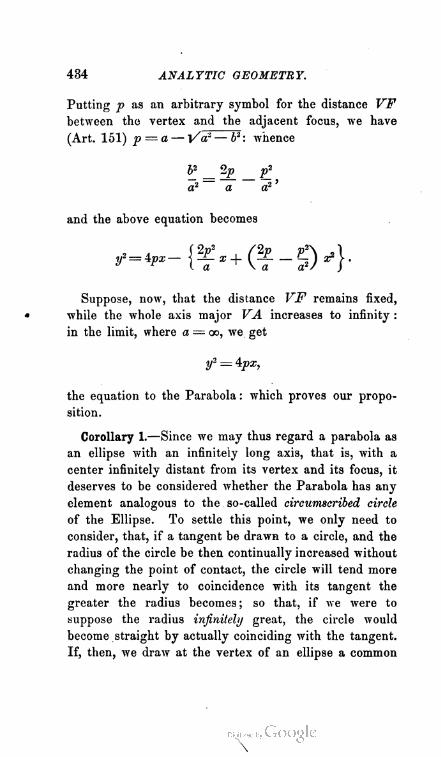
434 ANALYTIC GEOMETRY.
Putting p as an arbitrary symbol for the distance VF
between the vertex and the adjacent focus, we have
(Art. 151) p = a — Vdr — bl: whence
b2 2p p2
a2 a a2
and the above equation becomes
4
Suppose, now, that the distance VF remains fixed,
» while the whole axis major VA increases to infinity :
in the limit, where a = oo, we get
y2 = 4px,
the equation to the Parabola : which proves our propo
sition.
Corollary 1.—Since we may thus regard a parabola as
an ellipse with an infinitely long axis, that is, with a
center infinitely distant from its vertex and its focus, it
deserves to be considered whether the Parabola has any
element analogous to the so-called circumscribed circle
of the Ellipse. To settle this point, we only need to
consider, that, if a tangent be drawn to a circle, and the
radius of the circle be then continually increased without
changing the point of contact, the circle will tend more
and more nearly to coincidence with its tangent the
greater the radius becomes ; so that, if we were to
suppose the radius infinitely great, the circle would
become straight by actually coinciding with the tangent.
If, then, we draw at the vertex of an ellipse a common
\
ECCENTRICITY. 435
tangent to the curve and its circumscribed circle, and
subject the axis major to continual increase under the
conditions which will cause the curve to assume the form
of a parabola in the limit where a = oo, the circumscribed
circle will continually approach the common tangent as
its center recedes from the vertex, and, in the limit where
the ellipse vanishes into a parabola, will coincide with the
tangent. We learn, then, that the Parabola has an ana
logue of the circumscribed circle; that this analogue is
in fact the tangent of the curve at its vertex ; and that
it is also the line used as the axis of y in the equation
y2 — 4px, since this line and the tangent are both per
pendicular to the axis of the curve at its vertex, and
must therefore coincide. All these results will soon be
confirmed by analysis.
Corollary 2.—But, as a point of greater importance,
the relation established above enables us to assert that
the symbol e = 1 denotes the eccentricity of the corre
sponding parabola. For, in the Ellipse, we have
, a2 — b2 , P<? — — = 1 , ;
a2 a2
and if in this we make a = oo, or suppose the curve to
become a parabola, we get e — 1. That is, we may con
sider a parabola to be an ellipse in which the eccentricity
has reached the limit 1. Moreover, in the view taken
of this subject in the corollaries to Arts. 359, 456, the
condition e — 1 corresponds to that ellipse which has so
far deviated from the curvature of its circumscribed circle
as to vanish into the right line that forms its axis major.
Now, when we recollect (Art. 195, Cor.) that a right line
is a particular case of the Parabola, and that, in reaching
the limit 1, e has assumed a value fixed and the same
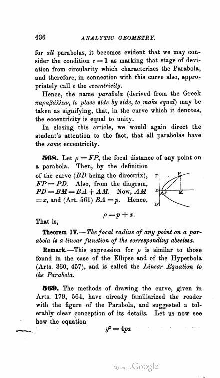
436 ANALYTIC GEOMETRY.
for all parabolas, it becomes evident that we may con
sider the condition e — 1 as marking that stage of devi
ation from circularity which characterizes the Parabola,
and therefore, in connection with this curve also, appro
priately call e the eccentricity.
Hence, the name parabola (derived from the Greek
napafidXteiv, to place side by side, to make equal) may be
taken as signifying, that, in the curve which it denotes,
the eccentricity is equal to unity.
In closing this article, we would again direct the
student's attention to the fact, that all parabolas have
the same eccentricity.
568. Let p = FP, the focal distance of any point on
a parabola. Then, by the definition
of the curve {BP being the directrix),
FP= PP- Also, from the diagram,
PD - BM=BA + AM. Now, AM
=x, and (Art. 561) BA —p. Hence,
p =p -f x.
That is,
Theorem IV.—The focal radius of any point on a par
abola is a linear function of the corresponding abscissa.
Remark.—This expression for p is similar to those
found in the case of the Ellipse and of the Hyperbola
(Arts. 360, 457), and is called the Linear Equation to
the Parabola.
569. The methods of drawing the curve, given in
Arts. 179, 564, have already familiarized the reader
with the figure of the Parabola, and suggested a tol
erably clear conception of its details. Let us now see
how the equation
y* = \px
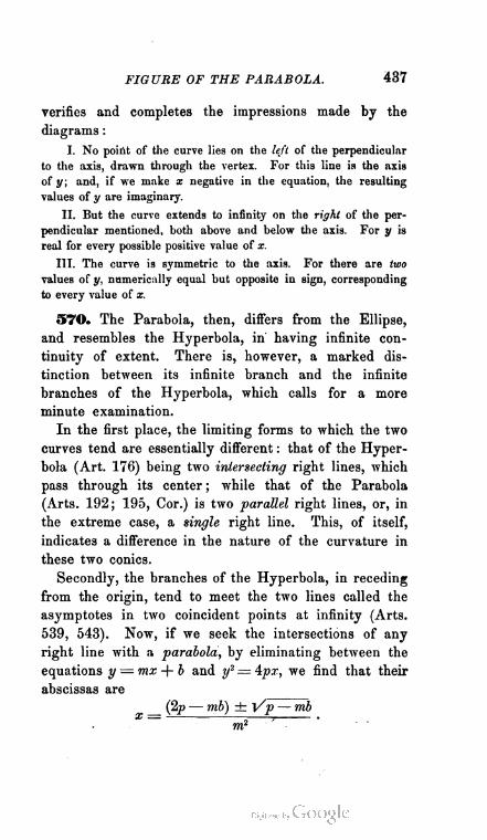
FIGURE OF THE PARABOLA. 437
verifies and completes the impressions made by the
diagrams :
I. No point of the curve lies on the left of the perpendicular
to the axis, drawn through the vertex. For this line is the axis
of y; and, if we make x negative in the equation, the resulting
values of y are imaginary.
II. But the curve extends to infinity on the right of the per
pendicular mentioned, both above and below the axis. For y is
real for every possible positive value of x.
III. The curve is symmetric to the axis. For there are two
values of y, numerically equal but opposite in sign, corresponding
to every value of x.
570. The Parabola, then, differs from the Ellipse,
and resembles the Hyperbola, in having infinite con
tinuity of extent. There is, however, a marked dis
tinction between its infinite branch and the infinite
branches of the Hyperbola, which calls for a more
minute examination.
In the first place, the limiting forms to which the two
curves tend are essentially different : that of the Hyper
bola (Art. 176) being two intersecting right lines, which
pass through its center ; while that of the Parabola
(Arts. 192; 195, Cor.) is two parallel right lines, or, in
the extreme case, a single right line. This, of itself,
indicates a difference in the nature of the curvature in
these two conies.
Secondly, the branches of the Hyperbola, in receding
from the origin, tend to meet the two lines called the
asymptotes in two coincident points at infinity (Arts.
539, 543). Now, if we seek the intersections of any
right line with a parabola, by eliminating between the
equations y — mx + b and y1 = 4px, we find that their
abscissas are
(2p — mb) ± l/p — mbx — , .
mr

438 ANALYTIC GEOMETRY.
In order, then, that these intersections may be coinci
dent, we must have mb — p : in which case, for the
abscissas, Ave get
* = A (1),ni-
and, for the equation to the given line,
y= mx-\- — ; or, m2x— my-\-p = 0 (2).
If, now, the coincidence takes place at infinity, we shall
have, from (1), ni — O; and (2) will assume the form
(Art. 110)
(7=0.
That is, any right line that tends to meet a parabola in
two coincident points at infinity, is situated altogether at
infinity; or, what is the same thing, no parabola has any
tendency to approach a finite right line in the manner
characteristic of the Hyperbola.
DIAMETERS.
571. Equation to any Diameter.—In a system of
parallel chords in a parabola, let 6 be the common in
clination to the axis, xy the middle point of any member
of the system, and x'y' the point in which the chord cuts
the curve. We have (Art. 101, Cor. 3)
x' = x — I cos d, y' =y — I sin 0.
Hence, as x'y' is on the parabola mentioned,
(y — I sin d)2 = \p (x — I cos 0).
That is, for determining I, we get the quadratic
Psin2 0 — 2 (y sin 0 — 2p cos 6) I = 4px — y2.
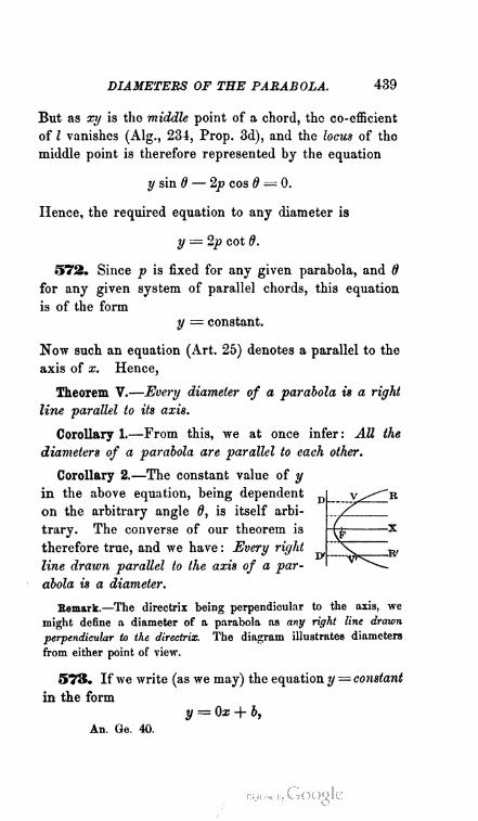
DIAMETERS OF THE PARABOLA. 439
But as xy is the middle point of a chord, the co-efficient
of I vanishes (Alg., 234, Prop. 3d), and the locus of the
middle point is therefore represented by the equation
y sin 0 — 2p cos 0 — 0.
Hence, the required equation to any diameter is
y — 2p cot d.
572. Since p is fixed for any given parabola, and d
for any given system of parallel chords, this equation
is of the form
y = constant.
Now such an equation (Art. 25) denotes a parallel to the
axis of x. Hence,
Theorem V.—Every diameter of a parabola is a right
line parallel to its axis.
Corollary 1.—From this, we at once infer: All the
diameters of a parabola are parallel to each other.
Corollary 2.—The constant value of y
in the above equation, being dependent
on the arbitrary angle 0, is itself arbi
trary. The converse of our theorem is
therefore true, and we have : Every right
line drawn parallel to the axis of a par
abola is a diameter.
Remark.—The directrix being perpendicular to the axis, we
might define a diameter of a parabola as any right line drawn
perpendicular to the directrix. The diagram illustrates diameters
from either point of view.
573. If we write (as we may) the equation y = constant
in the form
y — Oz + b,
An. Ge. 40.

440 ANALYTIC GEOMETRY.
and then eliminate y between it and y2 = 4px, we get,
for determining the intersections of a parabola with its
diameter, the relation Ox2 + Ox + b2 = 4px ; or,
Ox2 — 4px + b2=0.
Now (Alg., 238) the roots of this quadratic are
b2
4p
whence, observing the form of these roots, we have
Theorem VI,—Every diameter of a parabola meets the
curve in two points, one finite, the other at infinity.
Remark.—The meaning of this theorem, in ordinary geometric
language, is, of course, that a diameter only meets the curve in the
one finite point whose abscissa = V: 4p. The argument and the
phraseology adopted here are only used for the purpose of com
pleting analogies, and will seem less forced when we approach the
subject from a more generic point of view.
574. From the last theorem, it follows that no chord
of a parabola can be parallel to the axis, and, therefore,
that no diameter can bisect a system of chords parallel
to a second diameter. We thus learn, that, in the Par
abola, the conception of conjugate diameters vanishes in
the parallelism of all diameters.
THE TANGENT.
575. Equation to any Chord.—If x'y', x"y" be the
extremities of any chord in a parabola, we shall have
y'2 = 4px' and y"2— 4px". Hence, y"2—y'2=4p (x"—a/),
and we get
y"—y' _ 4p
x"— z> ~ y' + y"'
TANGENT OF THE PARABOLA. 441
Substituting this value for the second member of the
equation in Art. 95, we obtain the equation now re
quired, namely,
y — y' = *p
x — x' 1/ + y"
576. Equation to the Tangent.—Making y" = y'
in the preceding equation, reducing, and recollecting
that y'2 = ipx1, we get
y'y = 2p (x + x1).
577. Condition that a Right Line shall touch a
Parabola.—We have seen, in the second part of Art.
570, that y = mx + b will meet the parabola y2 = 4px in
two coincident points, whenever mb=p. The condition
now required is therefore
b = P.
m
Corollary.—Every right line, then, whose equation is
of the form
y = mx + —
m
is a tangent to tbe parabola y2 = \px. We have here
another instance of the so-called Magical Equation to the
Tangent.
578. Problem.—If a tangent to a parabola passes
through a fixed point, to find the co-ordinates of contact.
Putting x'y' for the required point of contact, and
x"y" for the fixed point through which the tangent
passes, we have (Arts. 563, 576)
= ipx1, y'y" = 2p (x1 + x").
442 ANALYTIC GEOMETRY.
Solving these conditions for x1 and y', we get
t_ (y"2 — ggg") ± y" Vy"'1 — ±px"
y'= y" ± Vy"'1 — 4px".
Corollary.—These values indicate that from any given
point two tangents can be drawn to a parabola : real
when y"2 — 4px" > 0, that is, when the point is without
the curve; coincident when y"2— £px" = Q, that is, when
the point is on the curve ; imaginary when y"2 —4px"< 0,
that is, when the point is within the curve.
579. Definition.—The halves of the chords which any
diameter of a parabola bisects, are called the ordinates
of the diameter. The term is also applied at times to
the entire chords, or to the right lines formed by pro
longing them indefinitely.
580. Let x'y' be the extremity of any parabolic di
ameter. Then, from Art. 571, y' — 2pcotd ; and we get,
for determining the angle 6 which the ordinates of the
diameter make with the axis,
tan 0 — .
y
Now the equation to the tangent at x'y' (Art. 576) may
be written
y = y (* + aO-
Hence, by the principle of Art. 78, Cor. 1,
Theorem VII.—The tangent at the extremity of any
diameter of a parabola is parallel to the corresponding
ordinates.

DIRECTION OF THE TANGENT. 443
Corollary.—Hence, further, the tangent at the vertex
of the curve is perpendicular to the axis ; and we confirm
by analysis the result of Art. 567, Cor. 1, namely, The
vertical tangent and the axis of y are identical.
581. The equations to any tangent of a parabola and
its focal radius of contact (Arts. 576, 95) may be written
y'y = >2p{x + x') (PT),
y'* + (p-*)y=py (FP).
For the angle FPT between these
lines, we therefore have (Art. 96,
Cor. 1)
tyy —yip—A y
But, by Art. 580, this is also the value of tan QPT.
Hence FPT= QPT; and we get
Theorem VIII.— The tangent of a parabola bisects the
internal angle between the diameter and focal radius drawn
to the point of contact.
Corollary 1.—To draw, then, a tangent to a parabola
at any point P, we form the focal radius PF, and the
diameter MP. We next prolong RP until PQ equals
PF, join QF, and draw PT perpendicular to QF: it
will be the tangent required, by virtue of the theorem
just proved, and the isosceles triangle FPQ.
Corollary 2.—Since SPR=QPT=FPT, all rays that
strike the concave of the curve in lines parallel to the
axis will be reflected to F, which is therefore called the
focus, as in the Ellipse and the Hyperbola.
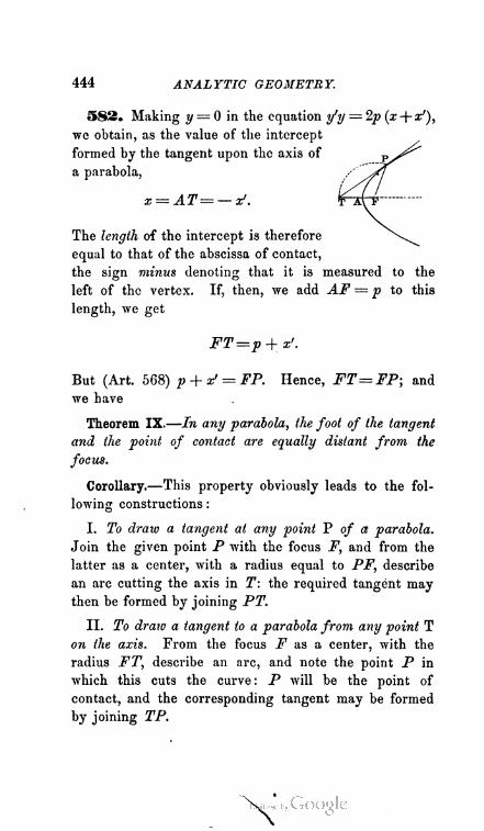
444 ANALYTIC GEOMETRY.
5S2. Making y — 0 in the equation
we obtain, as the value of the intercept
formed by the tangent upon the axis of
a parabola,
x = AT= — x'.
The length of the intercept is therefore
equal to that of the abscissa of contact,
the sign minus denoting that it is measured to the
left of the vertex. If, then, we add AF = p to this
length, we get
FT=p-+ x'.
But (Art. 568) p + x' = FP. Hence, FT=FP; and
we have
Theorem IX.—In any parabola, the foot of the tangent
and the point of contact are equally distant from the
focus.
Corollary.—This property obviously leads to the fol
lowing constructions :
I. To draw a tangent at any point P of a parabola.
Join the given point P with the focus F, and from the
latter as a center, with a radius equal to PF, describe
an arc cutting the axis in T: the required tangent may
then be formed by joining PT.
II. To draw a tangent to a parabola from any point T
on the axis. From the focus F as a center, with the
radius FT, describe an arc, and note the point P in
which this cuts the curve: P will be the point of
contact, and the corresponding tangent may be formed
by joining TP.
X

SUBTANGENT OF THE PARABOLA. 445
583. The Subtangent.—For the length of the sub-
tangent of the curve in the Parabola,
or of that portion of the axis which is Vy^^
included between the foot of the tan-
gent and that of the ordinate of con- y^f
tact, we have TM= TA+ AM; or, ^ Al »
subtan = z? + z' — 2x'.
584. Thus TA = AM= J TM, and we get the im
portant property,
Theorem X.—The subtangent of a parabola is bisected
in the vertex.
Corollary 1.—"We can now construct the tangent at
any point of the curve or from any point on the axis, as
follows : —When the point of contact P is given, draw
the ordinate PM, and on the prolonged axis lay off
AT'— AM: then, by the theorem just proved, T will
be the foot of the tangent at P, which is found by
joining PT.
When the foot T of the tangent is given, lay off upon
the axis AM— AT, and erect the ordinate MP. The
point P in which this meets the curve, will be the point
of contact sought ; and the tangent is obtained by join
ing TP.
Corollary 2.—As the value of the subtangent is depend
ent upon the peculiar form of the equation to the Para
bola, the present theorem is peculiar to this curve, and
hence leads to the following mode of constructing it,
which is often used by mechanics and draughtsmen.
Lay down two equal right lines AB, AC making any convenient
angle with each other. Bisect them in E and F, join EF, BC, and
draw AX perpendicular to the latter: it will bisect EF in V, and
BC in X, by the well-known properties of the isosceles triangle.

446 ANALYTIC GEOMETRY.
Now divide AE and its equal EB into the same number of equal
parts, and the equals AF, FO in the
same manner: the whole lines A B, A C
will thus be subdivided into equal parts Jrr^
at the points 1, 2, 3, E, 4, 5, 6 and 6, 5, 'i^Cf
4, F, 3, 2, 1. Having numbered these \^\X/>
points in reverse order upon the two A<~~><j")><9(y-
lines, as in the diagram, join those which ^^\)\ \
have the same numeral : the resulting ^SwV
lines will envelope a parabola, which s^V
we can approximate as closely as we r
please, by continually diminishing the
distances Al, 1.. .2, etc. For, by the construction, V is the middle
point of AX; and the curve touches all the lines AB, AC, 1 ... 1 ,
6 ... 6, etc. : hence, with respect to the lines AB, A C, which may
be regarded as limiting cases of all the others, it is a curve that
bisects Its subtangent in the vertex ; that is, a parabola.
From another point of view, the curve here formed is the envel
ope of a line EF, which moves within the fixed lines AB, AC in
such a manner that the sum of the remaining sides of the triangle
EAF is constant, being equal to AB. It is therefore a parabola,
by the result of the Example solved in Art. 251.
585. Perpendicular from the Focus to any Tan
gent.—For the length of the perpendicular from the focus
(p, 0) upon the line y'y — 2p [x + a/), we have (Art. 105,
Cor. 2)
2p(p + a/) _ 2p(p + x') ,/^T—rV)
\/(ip2 + yn) i/{4p(p + z')} ^P ;"
But (Art. 568) p-{-x'—p, the focal distance of the point
of contact. Hence,
P2=pp.
5S6. In this expression, p being constant, it is evident
that P2 will change its value as p changes its value ; or,
P will change with the square root of p : a property
usually expressed by
FOCAL PERPENDICULAR ON TANGENT. 447
Theorem XI.—The focal perpendicular upon the tangent
of a parabola varies in the subduplicate ratio of the focal
radius of contact.
587. Focal Perpendicular In terms of Its inclination to
tbe Axis.—The perpendicular from (p, 0) upon the line whose
equation (Art. 577, Cor.) is
rrfx — my -\- p = 0,
will be, according to Art. 105, Cor. 2,
P= fP + P P-VT+^.
V (m -f- m ) m
Put 6 = the inclination of P, measured from the axis toward the
right : then m = cot 0, and we get
P—p sec
588. The equation to the tangent being written (Art.
577, Cor.)
my — m2x =p,
that of its focal perpendicular, which passes through
O, 0), will be
my + x = p.
Combining these so as fo eliminate m, we get
x = 0
as the equation to the locus of the point in which the
focal perpendicular meets the tangent. Hence, (Art.
580, Cor.,)
Theorem XII.—The locus of the foot of the focal per
pendicular upon any tangent of a parabola, is the tangent
at the vertex of the curve.
Corollary 1.—By means of this property, we can solve
in its most general form the problem,
An. Ge. 41.

448 ANALYTIC GEOMETRY.
To draw a tangent to a parabola through any given
point. — Let P be the given
point, and join it with the focus
F. On PF as a diameter, de
scribe a circle cutting the ver
tical tangent in Q and Q' : these
points will be the feet of focal
perpendiculars, as the angles
PQF, PQ'F are inscribed in
semicircles. Hence, a line join
ing P to either of them, for instance the line PQ, will
touch the parabola in some point T.
If the point of contact is required, produce the axis to
meet PQ in R, and then apply the method of Art. 582,
Cor. When the given point is on the curve, as at T, the
auxiliary circle will touch the vertical tangent ; but the
point Q can still be found, by dropping a perpendicular
from the middle point of FT upon AY.
Corollary 2.—The present theorem, and the resulting
construction, completely justify the view, taken in Art.
567, Cor. 1, that the vertical tangent of the Parabola is
the analogue of the circle circumscribed about the Ellipse.
We thus arrive at the conclusion, often serviceable in anal
ysis, that the Right Line may be defined as the circle whose
radius is infinite.
589. Since the vertical tangent is the locus of the foot
of the focal perpendicular on any other tangent, that is,
the line in which the foot of every such perpendicular is
found, it follows that every right line drawn from the
focus to the vertical tangent is a focal perpendicular to
some other tangent of the curve. Besides, it is obvious
that any given point and right line may be regarded as
the focus and vertical tangent of some parabola. Hence,
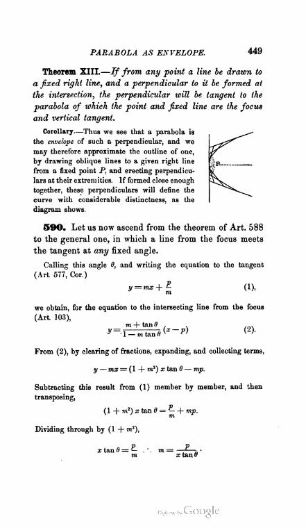
PARABOLA AS ENVELOPE. 449
Theorem XIII.—If from any point a line be drawn to
a fixed right line, and a perpendicular to it be formed at
the intersection, the perpendicular will be tangent to the
parabola of which the point and fixed line are the focus
and vertical tangent.
Corollary—Thus we see that a parabola is
the envelope of such a perpendicular, and we
may therefore approximate the outline of one,
by drawing oblique lines to a given right line
from a fixed point P, and erecting perpendicu
lars at their extremities. If formed close enough
together, these perpendiculars will define the
curve with considerable distinctness, as the
diagram shows.
590. Let us now ascend from the theorem of Art. 588
to the general one, in which a line from the focus meets
the tangent at any fixed angle.
Calling this angle 0, and writing the equation to the tangent
(Art. 577, Cor.)
y = mx+m (J)<
we obtain, for the equation to the intersecting line from the focus
(Art. 103),
m + tanff . . .
3 1 — mtantf v ^' v '
From (2), by clearing of fractions, expanding, and collecting terms,
y — mx — ( 1 + m2) x tan 6 — mp.
Subtracting this result from (1) member by member, and then
transposing,
P(1 + m2) x tan 8 = — + mp.
m
Dividing through by (1 + m2),
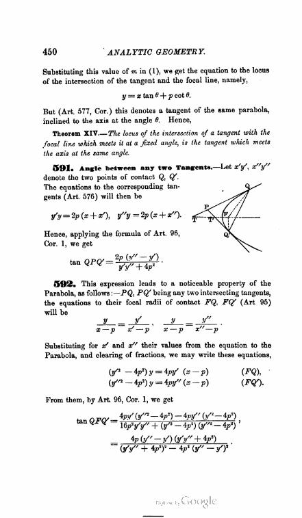
450 ANALYTIC GEOMETRY.
Substituting this value of m in (1), we get the equation to the locus
of the intersection of the tangent and the focal line, namely,
y = x tan 6 + p cot 0.
But (Art. 577, Cor.) this denotes a tangent of the same parabola,
inclined to the axis at the angle 6. Hence,
Theorem XIV—The locus of the intersection of a tangent with the
focal line which meets it at a fixed angle, is the tangent which meets
the axis at the same angle.
591. Angle between any two Tangents.—Let x'y', x"y"
denote the two points of contact Q, Of.
The equations to the corresponding tan
gents (Art. 576) will then be
y'y = 2p(x + x'\ y"y = 2p (x + x").
Hence, applying the formula of Art. 96,
Cor. 1, we get
2p Q/'-yQ
tan QPQf-
y'y" + W
592. This expression leads to a noticeable property of the
Parabola, as follows :—PQ, PQf being any two intersecting tangents,
the equations to their focal radii of contact FQ, FQf (Art. 95)
will be
y _y_ y
x —p x? —p
Substituting for x' and x" their values from the equation to the
Parabola, and clearing of fractions, we may write these equations,
ry -v)y =W (*•«).
{y>n _ V) y = 4py,, (x _ p) (W
From them, by Art 96, Cor. 1, we get
4p}f {y'n—V) — Apy" (y"— 4p2)
tan QFQf--\<Sfy'y" + (y» - 4p') (y"> - 4p>)
4p(y//-y,)(y,y// + ¥!)

NORMAL OF THE PARABOLA. 451
Now, if we apply the formula for the tangent of a double angle
(Trig., 847, m) to the angle QPQ', whose tangent we found in the
preceding article, we shall get, for the tangent of 2QPQ/, the ex
pression just obtained. Hence QFQ/ = 2QPQ/; and we have
Theorem XV.—The angle between any two tangents of a parabola
is equal to half the focal angle subtended by their chord of contact.
593. The equations to any two tangents of a parabola that cut
each other at right angles (Arts. 577, Cor. ; 96, Cor. 3) will be
i P xy = mx + — i y — mp.
m m
Subtracting the second of these from the first, we obtain
x — — p
as the equation to the locus of the intersection. But this equation
denotes a right line perpendicular to the axis at the distance p on
the left of the vertex; in other words, the line called the directrix
in our primary definitions. Hence,
Theorem XVI.—The locus of the intersection of tangents which cut
each other at right angles, is the directrix of the curve.
Corollary.—Since this locus, in the case of the Ellipse, is a circle
concentric with the curve (Art. 395), this theorem again shows us
that the Circle converges to the form of the Right Line as its radius
tends to infinity, and that we may therefore correctly regard the
Right Line as a circle with an infinite radius.
THE NORMAL.
594. Equation to the Normal.—The equation to
the perpendicular drawn through the point of contact
x'y' to the tangent
y'y = 2p(x + x'),
is found by Art. 103, Cor. 2, and is therefore
2p (y — y') = y' — x).

452 ANALYTIC GEOMETRY.
jr
595. Let P be any point x'y' on a parabola, PN the
corresponding normal, DP a diameter
through P, and jPP the focal radius
of its vertex. The equation to FP
(Art. 95) is
y'x—(x'—p)y=py'.
Comparing this with the equation to
the normal, we get (Art. 96, Cor. 1)
y'--2p(x'—p) 2p
But, since every diameter is parallel to the axis, DPN—
PNX, and we have, from the equation to the normal,
tain DPN=— }L.
zp
Hence, FPN= 180° — DPN = QPN; and we obtain
Theorem XVII.—The normal of a parabola bisects the
external angle between the corresponding diameter and
focal radius.
Corollary.—To construct a normal at any point P of
the curve, we therefore draw the focal radius PF, and
the diameter DPQ, laying olf upon the latter PQ =PF,
and joining QF: then will PN, drawn perpendicular to
QF, bisect the angle FPQ, and for that reason be the
normal required.
596. Intercept of the Normal—Making y = 0 in
the equation of Art. 594, we obtain
x = AN— 2p + x'.
Corollary.—This result enables us to
construct a normal at any point of the
curve, or from any point on the axis.
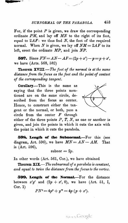
SUBNORMAL OF THE PARABOLA. 453
For, if the point P is given, we draw the corresponding
ordinate PM, and lay off MN to the right of its foot,
equal to 2AF: we thus find N, the foot of the required
normal. When N is given, we lay off NM= 2AF to its
left, erect the ordinate MP, and join NP.
597. Since FN=AN—AF= {2p +x')—p=p + x',
we have (Arts. 568, 582)
Theorem XVIII.—The foot of the normal is at the same
distance from the focus as the foot and the point of contact
of the corresponding tangent.
Corollary.—This is the same as
saying that the three points men
tioned are on the same circle, de
scribed from the focus as center.
Hence, to construct either the tan
gent or the normal, or both, pass a
circle from the center F through
either of the three points P, T, N, as one or another is
given, and join the points in which it cuts the axis with
the point in which it cuts the parabola.
598. Length of the Subnormal.—For this (see
diagram, Art. 596), we have MN= AN— AM. That
is (Art. 596),
subnor = 2p.
In other words (Art. 561, Cor.), we have obtained
Theorem XIX.— The subnormal of a parabola is constant,
and equal to twice the distance from the focus to the vertex.
599. Length of the Normal.—For the distance
between x'y' and (2p + x1 , 0), we have (Art. 51, I,
Cor. 1)
PN2 = 4p2 + yn = 4p (p + x').
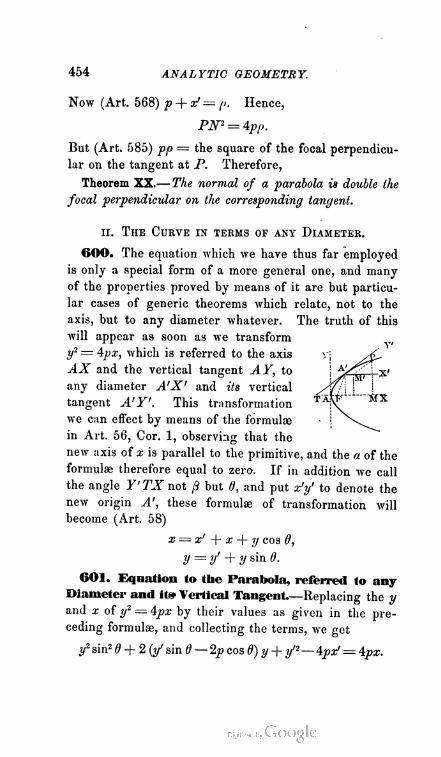
454 ANALYTIC GEOMETRY.
Now (Art. 568) p + x' — p. Hence,
pjSf2 = 4PP.
But (Art. 585) pp — the square of the focal perpendicu
lar on the tangent at P. Therefore,
Theorem XX.—The normal of a parabola is double the
focal perpendicular on the corresponding tangent.
u. The Curve in teems of any Diameter.
600. The equation which we have thus far employed
is only a special form of a more general one, and many
of the properties proved by means of it are but particu
lar cases of generic theorems which relate, not to the
axis, but to any diameter whatever. The truth of this
will appear as soon as we transform
y2 — 4px, which is referred to the axis
AX and the vertical tangent AY, to
any diameter A'X' and its vertical
tangent A'Y'. This transformation
we can effect by means of the formulas
in Art. 56, Cor. 1, observing that the
new axis of x is parallel to the primitive, and the « of the
formulae therefore equal to zero. If in addition we call
the angle Y' TX not ft but 0, and put x'y' to denote the
new origin A', these formulae of transformation will
become (Art. 58)
x = x' + £ + y cos d,
y = y' + y sin 0.
GOl. Equation to the Parabola, referred to any
Diameter and it» Vertical Tangent.—Replacing the y
and x of y1 — 4px by their values as given in the pre
ceding formulae, and collecting the terms, we got
y2 sin2 6 -f 2 (y' sin 6 — 2p cos 6) y + y'2— 4px! = 4px.

PARABOLA REFERRED TO ANY DIAMETER. 455
But, as the new origin x'y' is on the curve, y'2— 4j»a;'=0.
Also, since the new axis of y is a tangent, tan 6 = 2p : y' ;
so that y' sin# — 2p cos 6 — 0. Hence, the transformed
equation is in reality
y2 sin2 0 — 4px . (1).
Putting p : sin20—p', we may write the equation
y2 = \p'x (2).
This at once shows that yl = 4px is the form which (1)
assumes when the diameter chosen for the axis of x is
that whose vertical tangent is perpendicular to it, so
that sin2 0=1.
G02. Before employing our new equation itself, we
may extend the property of Theo
rem I by means of relations derived
from y2 — 4px : this will better pre
pare the way for the use of y2 — 4cp'x.
Let DA' be any diameter, and A' T
its vertical tangent. Parallel to the
latter, draw FF' through the focus.
Then, in the parallelogram F'T, we
shall have A'F' = FT = (Art. 582) FA'. But, from
the definition of the curve, supposing D'D to be the
directrix, FA' = A'D. Hence, A'D = A'F' ; or,
Theorem XXI.— The vertex of any diameter bisects the
distance from the directrix to the point in which the
diameter is cut by its focal ordinate.
603. The factor p' =p : sm!d which enters the second
member of equation (2), Art. 601, may be expressed in
terms of p and x', by the following process :
456 ANALYTIC GEOMETRY.
According to Art. 576, tan 0 — 2p : y'. Hence,
sin e- 2p - Vp ■
We have, then,
-JLj = p + x'.
sm-a
Now (Art. 568) p + x! = FA', the focal distance of the
vertex of any diameter. Hence,
Theorem XXII.—The focal distance of the vertex of any
diameter is equal to the focal distance of the principal
vertex, divided by the square of the sine of the angle between
the diameter and its vertical tangent.
604. The expression just obtained aids us to interpret
the new equation y2 = ip'x. For, from what precedes,
the equation may be written
y2 = 4 (p + x') x,
and we learn that the symbol p' signifies the focal
distance of the vertex taken for the new origin. We
therefore read from the equation at once, the following
extension of Theorem III :
Theorem XXIII.— The square on an ordinate to any
diameter is equal to four times the rectangle under the
corresponding abscissa and the focal distance of the
vertex.
Corollary.—Hence, the squares on the ordinates to
any diameter vary as the corresponding abscissas.

FOCAL DOUBLE ORDINATES. 457
605. In Art. 602, we found A'F' = FA' — p + x'.
Hence, making x ~p + x' in the equa
tion of Art. 604, we get
y=F'P= 2 (p + a/) = 2FA'.
Now, since every diameter bisects the <i\
chords parallel to its vertical tangent,
PQ = 2F'P=4FA'; and we have
Theorem XXIV.— The focal double ordinate to any
diameter is equal to four times the focal distance of its
vertex.
Remark.—The value of the latus rectum (Art. 566),
furnishes a particular case of this theorem ; and, as 4p
signifies the length of the focal double ordinate to the
axis, so 4p', by what precedes, represents that of the
focal double ordinate to any diameter. From Arts. 429,
522, we see that this uniform analogy among the focal
double ordinates to all diameters, is peculiar to the
Parabola.
606. The reader may now interpret the equation
y — ± 2Vfx,
and show by means of it, that, with reference to any
diameter, the Parabola consists of a single infinite
branch, tending to two parallel right lines as its limiting
form, and symmetric to the diameter.
DIAMETRAL PROPERTIES OP THE TANGENT.
607. Equation to the Tangent, referred to any
Diameter.—From the identity of form in the equations
y2 = 4px, y2 = 4p'x, we at once infer that this must be
y'y = 2p' (x + x').

458 ANALYTIC GEOMETRY.
GOS. Making y = 0 in this equation, wc get, for the
intercept of the tangent on any diameter,
x =— x'.
This shows that the tangent cuts any diameter on the
left of its vertex, at a distance equal to the abscissa of
contact. Thus the vertex of any diameter is situated
midway between the foot of the tangent and that of its
ordinate of contact, and we have, as the extension of
Theorem X,
Theorem XXV.—The subtangent to any diameter of a
parabola is bisected in the corresponding vertex.
Corollary 1.—This property enables us to construct a
tangent to a parabola from any P
external point whatever. For, if ^^/ '>
T' be such point, we have only ...■■"'yv,/k'—j
to draw the diameter T'M', form —JlZLZ. ^
the tangent A'T at its vertex V
(by dropping a perpendicular
from A' upon the axis, and
setting off AT = the abscissa thus determined), take
A'M' = A'T', draw M'P parallel to the tangent A'T,
and join FT'.
Corollary 2.—By the same property, we can construct
an ordinate to any diameter. This is either done in the
way M'P was formed above, or as follows:—Take any
point T" on the axis, make AM— AT", erect the per
pendicular MP, and join PT". Then, T' being the
point where this tangent cuts the given diameter, take
A'M' = A' T', and join M'P.
609. Let PQ be any chord of a parabola. Then
(Art. 607) the equations to the tangents at its opposite
POLAR IN THE PARABOLA. 459
extremities P and Q, by referring them to its bisecting
diameter, will be
2p' (x + O —y'y = 0, 2p' (x + x>) + y'y = 0.
Subtracting the first of these from the second, we get
y = 0
as the equation to the locus of the intersection. Hence,
Theorem XXVI.—Tangents at the extremities of any
chord of a parabola meet on the diameter which bisects
that chord.
POLE AND POLAR.
610. We shall now prove that the polar relation is a
property of the Parabola, following the same steps as in
the Ellipse and the Hyperbola.
611. Chord of Contact in the Parabola.—Let x'y'
denote the point from which the two tangents that deter
mine the chord are drawn, and xjyt the extremities
of the chord. Since x'y' is upon both tangents, we have
M' =V + xd> yiy' = 2p' (x' + x2).
That is, the two extremities of the chord are on the line
whose equation is
y'y = 2p' (x + x').
And this is therefore the equation to the chord itself.
612. Locus of the Intersection of Tangents to the
Parabola.—Let x'y' be the fixed point through which
the chord of contact of the intersecting tangents is drawn.
Then, if a?,^, be the intersection of the two tangents, since
x'y' is always on their chord of contact, we shall have
(Art. 611)
yxy' = 2p' (x' + a;,).
460 ANALYTIC GEOMETRY.
And this being true, however xlyl may change its position
as the chord of contact revolves about x'y', the co-ordi
nates of intersection must always satisfy the equation
y'y = 2p' (x + x').
This, therefore, is the equation to the locus sought.
613. Tangent and Chord of Contact taken np
into the wider conception of the Polar.—Here, too,
as well as in the Ellipse and the Hyperbola, the two
equations just found are identical in form with that of
the tangent. By the same reasoning, then, as in Arts.
433, 526, we learn that the tangent and chord of contact
in the Parabola are particular cases of the locus just dis
cussed. Now, too, by its equation, this locus is a right
line ; and, if we suppose x'y' to be any point on a given
right line, the co-efficients of the equation in Art. 611
will fulfill the condition Ax' + By' + C— 0, and thus
(Art. 117) the chord of contact will pass through a fixed
point. In the curve now before us, therefore, we have
the twofold theorem :
I. Iffrom a fixed point chords be drawn to any para
bola, and tangents to the curve be formed at the extremities
of each chord, the intersections of the several pairs of tan
gents will lie on one right line.
II. Iffrom different points lying on one right line pairs
of tangents be drawn to any parabola, their several chords
of contact will meet in one point.
Thus the law that renders the locus of Art. 612 the
generic form of which the tangent and chord of contact
are special phases, is the law of polar reciprocity : whence
the Parabola, in common with the other two Conies, im
parts to every point in its plane the power of determining
a right line ; and reciprocally.

POLAR IN THE PARABOLA. 461
614. Equation to the Polar with respect to a
Parabola.—This, as we gather immediately from the
preceding results, is
y'y = 2p' (x + x%
if referred to any diameter; or, if referred to the axis,
y'y = 2p{x + x').
615. Definitions.—The Polar of any point, with re
spect to a parabola, is the right line which forms the
locus of the intersection of the two tangents drawn at
the extremities of any chord passing through the point.
The Pole of any right line, with respect to the same
curve, is the point in which all the chords of contact
corresponding to different points on the line intersect.
We have, then, the following constructions : —When
the pole P is given, draw through it
any two chords T'T, S'S, and form
the corresponding pairs of tangents,
T'L and TL, S'M and SM: the line
LM which joins the intersection of
the first pair to that of the second,
will be the polar of P. When the
polar is given, take any two of its
points, as L and M, draw a pair of tangents from each,
and form the corresponding chords of contact, T'T, S'S:
the point P in which these intersect, will be the pole of
LM.
When the pole is without the curve, as at M, the polar
is the corresponding chord of contact S'S; and when it
is on the curve, as at T, the polar is the tangent at T.
In these cases, the drawing may be made in accordance
with the facts.

462 ANALYTIC GEOMETRY.
616. Direction of the Polar.—By referring the
polar of any point to the diameter drawn through the
point, the y' of its equation will become = 0, and the
equation itself (Art. 614) will assume the form
x = — x'.
This denotes a parallel to the axis of y. Hence,
Theorem XXVII.—The polar of any point, with respect
to a parabola, is parallel to the ordinates of the diameter
which passes through the point.
Corollary 1.—The equation x = — x', more exactly
interpreted, gives us : The polar of any point on a
diameter is parallel to the ordinates of the diameter, and
its distance froni the vertex of the diameter is equal, in an
opposite direction, to the distance of the point. And, in
particular, The poldr of any point on the axis is the per
pendicular which cuts the axis at the same distance from
the vertex as the point itself, but on the opposite side.
Corollary 2.—To construct the polar, therefore, draw
a diameter through the pole, take on the opposite side
of its vertex a point equidistant with the pole, and draw
through this a parallel to the corresponding ordinates.
617. Polar of the Focus.—The equation to this is
obtained by putting (p, 0) for x'y' in the second equation
of Art. 614, and is
x = — p.
The focal polar of the Parabola is therefore identical
with the line which in Art. 180 we named the directrix,
and we shall presently see that our ability to generate
the curve by the means employed in Art. 179, is due to
the polar relation of that line to the focus.
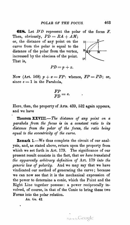
POLAR OF THE FOCUS. 463
618. Let jyi) represent the polar of the focus F.
Then, obviously, PD = RA + AM;
or, the distance of any point on the d
curve from the polar is equal to the
distance of the polar from the vertex, R
increased by the abscissa of the point.
That is, " V
PD=p + x.
Now (Art. 568) p + x = FP: whence, FP = PD; or,
since e = 1 in the Parabola,
FP _PD~e-
Here, then, the property of Arts. 439, 532 again appears,
and we have
Theorem XXVIII.—The distance of any point on a
parabola from the focus is in a constant ratio to its
distance from the polar of the focus, the ratio being
equal to the eccentricity of the curve.
Remark 1.—We thus complete the circuit of our anal
ysis, and, as stated above, return upon the property from
which we set forth in Art. 179. The significance of our
present result consists in the fact, that we have translated
the apparently arbitrary definition of Art. 179 into the
generic law of polarity. And we may say that we have
vindicated our method of generating the curve ; because
we can now see that it is the mechanical expression of
the power to determine a conic, which the Point and the
Right Line together possess : a power reciprocally in
volved, of course, in that of the Conic to bring these two
Forms into the polar relation.
An. Ge. 42.
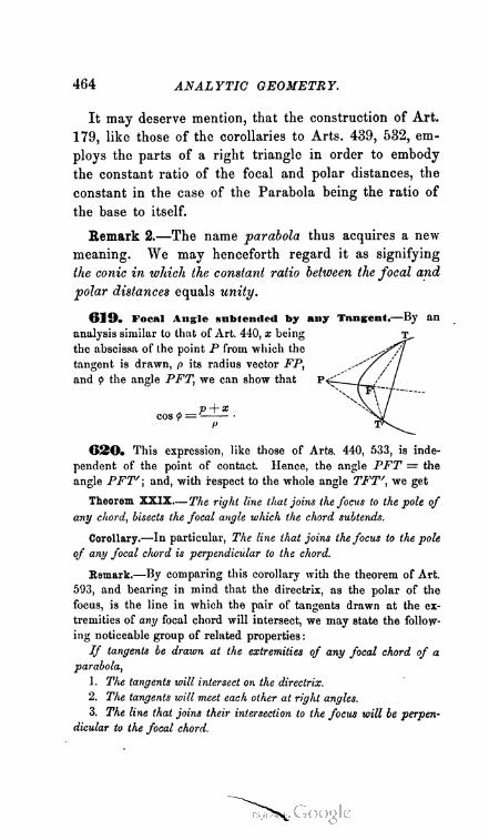
464 ANALYTIC GEOMETRY.
It may deserve mention, that the construction of Art.
179, like those of the corollaries to Arts. 439, 532, em
ploys the parts of a right triangle in order to embody
the constant ratio of the focal and polar distances, the
constant in the case of the Parabola being the ratio of
the base to itself.
Remark 2.—The name parabola thus acquires a new
meaning. We may henceforth regard it as signifying
the conic in which the constant ratio between the focal and
polar distances equals unity.
61 0. Focal Angle subtended by any Tangent.—By an
analysis similar to that of Art. 440, x being
the abscissa of the point P from which the
tangent is drawn, p its radius vector FPt
and <? the angle PFT, we can show that P
p + xcos ? = ■
I'
620. This expression, like those of Arts. 440, 533, is inde
pendent of the point of contact. Hence, the angle PFT = the
angle PFT'; and, with respect to the whole angle TFT', we get
Theorem XXIX—The right line that joins the focus to the pole of
any chord, bisects the focal angle which the chord subtends.
Corollary.—In particular, The line that joins the focus to the pole
of any focal chord is perpendicular to the chord.
Remark.—By comparing this corollary with the theorem of Art.
593, and bearing in mind that the directrix, as the polar of the
focus, is the line in which the pair of tangents drawn at the ex
tremities of any focal chord will intersect, we may state the follow
ing noticeable group of related properties :
If tangents be drawn at the extremities of any focal chord of a
parabola,
1. The tangents will intersect on the directrix.
2. The tangents will meet each other at right angles.
3. The line that joins their intersection to the focus will be perpen
dicular to the focal chord.
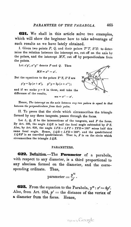
PARAMETER OF THE PARABOLA. 465
621. We shall in this article solve two examples,
which will show the beginner how to take advantage of
such results as we have lately obtained.
I. Given two points P, Q, and their polars T'T, S'S: to deter
mine the relation between the intercept mn, cut off on the axis by
the polars, and the intercept MN, cut off by perpendiculars from
the points.
Let x'y', x"y" denote P and Q. Then
MN=x" -x'.
But the equations to the polars 2" T, S'S are
y'y--=2p(x+ x'), y"y=2p{x + x");
and if wo make y = 0 in these, and tako the
difference of the results,
mn = x" — x' .
Hence, The intercept on the axis between any two polars is equal (o that
between the perpendiculars from, their poles.
II. To prove that the circle which circumscribes the triangle
formed by any three tangents, passes through the focus.
Let L, Q, R be the intersections of the tangents, and F the focus.
By Art. 592, the angle LQR is half the focal angle subtended by S'S.
Also, by Art. 620, the angle LFR = LFT+ TFR = 180° minus half this
same focal angle. Hence, LQR + LFR = 180°, and the quadrilateral
LQRF is an inscribed quadrilateral. That is, F is on the circle which
circumscribes the triangle L QR.
PARAMETERS.
622. Definition.—The Parameter of a parabola,
with respect to any diameter, is a third proportional to
any abscissa formed on the diameter, and the corre
sponding ordinate. Thus,
parameter = ~- .
623. From the equation to the Parabola, y'2 : xf= 4j)'.
Also, from Art. 604, p' = the distance of the vertex of
a diameter from the focus. Hence,

466 ANALYTIC GEOMETRY.
Theorem XXX.—The parameter of any diameter in a
parabola is equal to four times the focal distance of its
vertex.
Corollary.—The parameter of the axis, or, as it is
usually called, the principal parameter, is therefore
equal to four times the distance from the focus to the
vertex of the curve ; that is, its value is 4p.
Remark.—In the equations y2 — 4p'x, y2 = \px, we
are henceforward to understand that p' is one-fourth
the parameter of the reference-diameter, and p one-
fourth the parameter of the axis. Or, with greater
generality, in any equation of the form
f - P*,
P, the constant co-efficient of x, is to be interpreted
as the parameter of the corresponding parabola, taken
with respect to the diameter to which the equation is
referred.
624. In Art. 605, we proved that the focal double
ordinate to any diameter is equal to four times the focal
distance of its vertex. Hence,
Theorem XXXI.—The parameter of any diameter in
a parabola is equal to the focal double ordinate of that
diameter.
Corollary.—Accordingly, the parameter of the axis is
equal to the lotus rectum: as we might also infer from
the fact that both are equal to 4p.
Remark.—From Arts. 429, 522, as already noticed in
another connection, we see that the Parabola is the only
conic in which the parameter of every diameter is equal
to the corresponding focal double ordinate.
PARABOLA REFERRED TO ITS FOCUS. 467
625. It is sometimes useful to express the parameter
of any diameter in terms that refer to the axis of the
curve as the axis of x. To effect this, we either use the
relation
p'=p + *? (1),
whei-e z' is the abscissa of the vertex of the diameter
whose parameter is sought, measured on the axis; or
else
n' — P '(2)
where 0 is the angle made with the axis by the tangent
at the vertex of the diameter.
626. The latter of the foregoing relations may be
interpreted as
Theorem XXXII.—The parameter of any diameter
varies inversely as the square of the sine of the angle
which the corresponding vertical tangent makes with the
axis.
in. The Curve referred to its Focus.
627. The polar equations to the Parabola (Art. 183
cf. Rem.) being
_ 2pP ~ 1 ± cos 0 '
our present knowledge leads us to assign to p its proper
meaning, and to describe the numerator in the value of p
as half the "parameter of the curve.
Moreover, since e — 1 in the Parabola, we may write

468 ANALYTIC GEOMETRY.
thus completely exhibiting the analogy of these ex
pressions to the corresponding elliptic equations of Art.
443 : an analogy which we partially established in Art.
184, and which verifies the proposition of Art. 567, that
a parabola may be regarded as an ellipse in which the
eccentricity has passed to the limiting value = 1.
C»US. Polar Equation to the Tangent.—In seeking
this, we shall avail ourselves of the property just men
tioned.'
If in the equation of Art. 444 we replace a (1 — e2)
by its value 2p, as found in Art. 443, we may write the
polar equation to an elliptic tangent
P =2p
cos (p — 0') — e cos 0
Making e — 1 in this, we get the equation to a ■parabolic
tangent, namely,
^ ; 2p_P cos (0 — 0') — cos 0 '
iv. Area of the Parabola.
629. The area of any parabolic segment, included
between the curve and any double ordinate to the axis,
may be computed as follows :
Supposing A-PMQ to be the segment
whose area is sought, divide its abscissa
AM into any number of equal parts at
B, C, I), . . . , erect ordinates BL, CN,
DR, ... at the points of division, and
through their extremities L, N, R, . . .
draw parallels to the axis, producing both
the ordinates and the parallels until they meet as in the

AREA OF THE PARABOLA. 469
figure. The curve divides the circumscribed rectangle
TJM into two segments : and, by the process just de
scribed, there will be formed in both of these a number
of smaller rectangles, corresponding two and two ; as
UR to EM, ON to ND, EL to LC, etc.
Let x'y', x"y" be any two successive points thus formed
upon the curve ; for instance, L, N. Then
area LC= y' (x» — af) =^^n~^ ,
area EL = x' (y" — y') = ~^ ■
To express, then, the ratio of any interior rectangle to
its corresponding exterior one, we shall have an equation
of the form
LC _ y" + y' _-,,y!
EL~ y> ~ + y' '
Hence, the limiting value to which this ratio tends as y"
converges to y', is evidently = 2 : and therefore the
ratio borne by the sum of the interior rectangles to the
sum of the exterior, also tends to the limit 2 as y" con
verges to y'. Now the condition that y" may converge
to y' is, that the subdivision of AM shall be continued
ad infinitum: and if this takes place, the sum of the in
terior rectangles will converge to the area of the interior
segment APM; and the sum of the exterior, to the area
of the exterior segment APU. Therefore, APM =
2APU; or, putting x = AM, y = MP, and A = the
area of the interior segment,

470 ANALYTIC GEOMETRY.
Similarly, the segment AQM= -xy: whence,
o
Theorem XXXIII.—TJie area of a parabolic segment
cut off by any double ordinate to the axis, is equal to
two-thirds of the circumscribing rectangle.
Corollary—Since the same reasoning is obviously
applicable to the equation y2 = ±p'x, we may at once
state the generic theorem : The area of a parabolic seg
ment cut off by a double ordinate to any diameter, is equal
to two-thirds of the circumscribing parallelogram.
EXAMPLES ON THE PARABOLA.
1. The extremities of any chord of a parabola being x'y', x"y",
and the abscissa of its intersection with the axis being x, to prove
that
x'x" = x2, y'y"= — 4px.
2. Two tangents of a parabola meet the curve in x'y' and x"y" \
their point of intersection being xy, show that
x = Wx77, y - ■
3. The area of the triangle formed by three tangents of a para
bola is half that of the triangle formed by joining their points of
contact.
4. To prove that the area of the triangle included between the
tangents to the parabolas
y1 = mx, y2 = nx
at points whose common abscissa = a, and the portion of the cor
responding ordinate intercepted between the two curves, is equal to
1 13
5. To prove that the three altitudes of any triangle circum
scribed about a parabola, meet in one point on the directrix.

EXAMPLES ON THE PARABOLA. 471
6. The cotangents of the inclinations of three parabolic tangents
are in arithmetical progression, the common difference being = <5:
prove that, in the triangle inclosed by these tangents, we shall have
area = p'1^3.
7. Given the outline of a parabola: to construct the axis and
the focus.
8. Find the equation to the normal of a parabola, in terms of
its inclination to the axis; and prove that the locus of the foot of
the focal perpendicular upon the normal is a second parabola, whose
vertex is the focus of the given one, and whose parameter is one-
fourth as great as that of the given one.
9. Show that the locus of the intersection of parabolic normals
which cut at right angles, is a parabola whose parameter is one-
fourth that of the given one, and whose vertex is at a distance = Sp
from the given vertex.
10. The centers of a series of circles which pass through the
focus of a parabola, are situated on the curve: prove; that each
circle touches the directrix.
11. To find the area of the rectangle included by the tangent
and normal at any point P of a parabola, and their respective focal
perpendiculars ; and to determine the position of P when the rect
angle is a square.
12. If two parabolic tangents are intersected by a third, parallel
to their chord of contact, the distances from their point of intersec
tion to their respective points of contact are bisected by the third
tangent.
13. Show that the locus of the vertex of a parabola which has
a given focus, and touches a given right line, is a circle, of which
the perpendicular from the given focus to the given line is a diameter.
14. Show that, if a parabola have a given vertex, and touch a
given right line, its focus will move along another parabola, whose
axis passes through the given vertex at right angles to the given
line, and whose parameter = the distance from the given vertex
to the given line.
15. TP and TQ are tangent to a given parabola at P and Q,
and TF joins their intersection to the focus: prove that
FP. FQ = FT2.
An. Ge. 43.

472 ANALYTIC GEOMETRY.
16. A right angle moves in such a manner that its sides are
respectively tangent to two confocal parabolas whose axes are
coincident: to find the locus of its vertex.
17. Prove that the pole of the normal which passes through one
extremity of the latus rectum of a parabola, is situated on tiie diam
eter which passes through the other extremity, and find its exact
position on that line.
18. The triangle included by two parabolic tangents and their
chord of contact being of a given area = a2, prove that the locus
of the pole is a parabola whose equation is
y"- = ipx + (2po')*
19. Prove that, if two parabolas whose axes are mutually per
pendicular intersect in four points, the four points lie on a circle.
20. If two parabolas, having a common vertex, and axes at right
angles to each other, intersect in the point x'y': then, / denoting
the latus rectum of the one, and V that of the other,
I : X* : : y' : V.
[This property has a special interest, on account of its connection with
the ancient problem of the Duplication of the Cube. It affords, as the
reader will observe, a method of determining graphically two geometric
means between two given lines ; and was proposed for this purpose by
Menechmus, a geometer of the school of Plato, in connection with his
attempt to solve the problem just mentioned. The graphic problem of
"two means" received a variety of solutions at the hands of the Greek
geometers, two of the most celebrated being discovered by Diocles and
Nicomedes. They are effected, respectively, with the help of the curves
called the Cissoid and the Conchoid.]
CHAPTER SIXTH.
THE CONIC IN GENERAL.
630. Having in the previous Chapters become familiar
with the properties of the several conies considered as
THE CONIC IN GENERAL. 473
separate curves, let us now ascend to the wholly generic
point of view, from which we may comprehend them not
as isolated Forms, but as members of a united System,
and, in fact, as successive phases of a generic locus which
may be called the Conic, whose idea we sketched in the
eighth Section of Part I.
We may begin by showing in what sense this name is
descriptive of the system ; or, how the curves may be
grouped together as sections of a cone.
THE THREE CURVES AS SECTIONS OF THE CONE.
631. Definitions.—A Cone is a surface generated by
moving a right line which is pivoted upon a fixed point,
along the outline of any given curve whose plane does
not contain the fixed point.
The fixed point is called the vertex of the cone; the
given curve, its directrix; and the moving right line, its
generatrix.
Since the generatrix extends indefinitely on both sides
of the vertex, the cone will consist of two exactly similar
portions, extending from the vertex in opposite directions
to infinity. Of these, one is called the upper nappe of the
cone; and the other, the lower nappe.
Any single position of the generatrix is called an ele
ment of the cone.
When the directrix is a circle, the cone is called cir
cular; and the right line drawn through the vertex and
the center of the directrix, is termed the axis of the cone.
632. Definitions.—A Right circular Cone is a cone
whose directrix is a circle, and whose axis is perpendic
ular to the plane of its directrix.
The section formed with any cone by a plane, is
termed a base of the cone ; consequently, the directrix

474 ANALYTIC GEOMETRY.
of a right circular cone may be called its base. For
this reason, such a cone is often named a right cone on
a circular base. The diagram of the next article presents
an example of one.
633. We shall prove, in the proper place in Book
Second, tho following propositions, which we ask the
student to take upon trust for the present, in order that
we may use them in grouping the three curves according
to their geometric order :
I. Every section formed by passing a plane through
a right circular cone is a curve of the Second order.
II. If the angle which the secant plane makes with
the base is less than that made by the generatrix, the
section is an" ellipse.
III. If the angle which the secant plane makes with
the base is equal to that made by the generatrix, the
section is a parabola.
IV. If the angle which the secant plane makes with
the base is greater than that made by the generatrix,
the section is an hyperbola.
These three cases are represented
in the diagram : that of the Ellipse,
at AE; that of the Parabola, at
LPR; and that of the Hyperbola,
at HA- A'H'. It is manifest, how
ever, from the fact that the secant
plane makes with the base an angle
successively less than, equal to, and
greater than the angle made by the
generatrix (whose angle must have
a fixed value for any given cone),
that the three sections may be formed by a single

SECTIONS OF A CONE. 475
plane, by simply revolving it on the line in which it
cuts the base. Beginning with it in such a position
that its inclination to the base is less than that of the
generatrix (whose inclination is often called the incli
nation of the side of the cone), and revolving it upward
toward the position of parallelism to the side, we shall
cut out a series of ellipses of greater and greater
eccentricity. When the secant plane becomes parallel
to the side, the section will be a parabola. When it is
pushed still farther upward, so that its angle with the
base becomes greater than that of the side, it will reach
across the space between the two nappes of the cone,
and pierce the upper as well as the lower one, and the
section will be an hyperbola, whose two branches will
lie in the two nappes respectively.
From this it appears, that, granting the proposition
that the sections are the curves mentioned, the natural
geometric order in which they occur is : Ellipse, Para
bola, Hyperbola. This is the same as their analytic
order, as we found it in Art. 200. We shall be able to
give a more explicit account of their appearance as suc
cessive phases of the Conic, so soon as we have presented
a fuller view of the modes in which we can represent
that generic locus by analytic symbols.
VARIOUS FORMS OF THE EQUATION TO THE CONIC.
634. Equation in Rectangular Co-ordinates at
the Vertex.—We have not as yet referred the three
Conies to the same axes and origin : let us now do so,
by transforming the central equations of the Ellipse and
the Hyperbola to such a vertex of each curve as will
correspond to the vertex of the Parabola.

476 ANALYTIC GEOMETRY.
This will require us to transform the equation
to the left-hand vertex of the Ellipse; and the equation
f=~^~a2) (2)
to the right-hand vertex of the Hyperbola. Accordingly,
putting x — a for x in (1), and x + a for x in (2), and
expanding, we get
2 2b2 V t 2b2 , b2 2V = — a; a;2, ?r = — x A sr.J a a2 ' 9 a ^ a2
Hence, (Arts. 428, 521,) the equations to the Ellipse,
the Hyperbola, and the Parabola may be written
b2 b2y2= 4px——x2, y2 — 4px -f- — x2, y2 = 4px.
Remembering, now, that b2 : a2 = ± (1 — e2), and that its
value in the case of the Parabola must therefore be = 0,
we learn that the equation to the Conic in General is
y2 = Px + Rx2,
in which P is the parameter of the curve, and R the ratio
between the squares of the semi-axes; and we have the
specific conditions
R < 0 . • . Ellipse,
R = 0 . • . Parabola,
R > 0 . • . Hyperbola.
Corollary.—By the three equations from which y2 —
Px + Ri? was generalized, we see that in the Ellipse,

NAMES OF THE SECTIONS. 477
the square on the ordinate is less than the rectangle
under the abscissa and parameter; that in the Parabola,
the square is equal to the rectangle; and that in the
Hyperbola, the square is greater than the rectangle.
Kemark—According to Pappus (Math. Coll., VII: c. a. d. 350),
the names of the three curves were originally given to designate
this property. But Eutooius (a. d. 560) says that the names were
derived from the fact, that, according to the ancient Greek geome
ters, the three sections were cut respectively from an acute-angled,
a right-angled, and an obtuse-angled cone, by means of a plane
always passing at right angles to the side. Thus, if the angle
under the vertex of the cone were acute, the sum of that and the
right angle made by the secant plane with the side would be less
than two right angles, and the name ellipse was given, either to
indicate this deficiency, or to show that the curve would then fall
short of the upper nappe of the cone. But if the angle under the
vertex were right, the mentioned sum of angles would be equal to
two right angles, and the plane of the curve consequently be par
allel to the side of the cone: to denote which facts, the nsxme para
bola was given. Finally, if the angle under the vertex were obtuse,
the mentioned sum of angles would be greater than two right angles,
and the name hyperbola was given, either to suggest this excess, or
to indicate that the curve would then reach over to the upper nappe
of the cone.
It is noticeable here, that the early geometers supposed the three
sections to be peculiar respectively to an acute-angled, a right-angled,
and an obtuse-angled cone. The improvement of forming them all
from the same cone by merely changing the inclination of the secant
plane, was introduced by Apollonius op Perga, b. c. 250.
Which of these etymologies should have the preference, is a
question among critics of mathematical history. It is remarkable,
however, that the names represent equally well all the distinguish
ing properties of the curves, whether geometric or analytic : as the
reader may perhaps have already observed for himself
The name parameter, which simply means corresponding measure,
or co-efficient, is given to the quantities '2!r : a and yn : x', on account
of the position they occupy in the equation
ya = Px + Rx\
one or the other of them being the first co-efficient in the second
478 ANALYTIC GEOMETRY.
member, according as the conic is central or non-central. More
over, as the dimensions of the curve depend mainly upon the value
of P, the ratios which it symbolizes are naturally termed par excel
lence the measures of the Conic. On the other hand, the namo
parameter may be defined in each conic by the value which i;
denotes for each, as in the preceding Chapters.
635. Equation in terms of the Focus and its
Polar.—We have seen (Arts. 439, 532, 618) that in
every conic the distance of any point on the curve from
the focus is in a constant ratio to its distance from the
polar of the focus, the ratio being equal to the eccen
tricity. Hence, calling the focal distance p, and the
distance from the polar (or directrix) 8, we may write,
as the equation to the Conic,
p = e.d:
which will denote an ellipse, a parabola, or an hyperbola,
according as e is less than, equal to, or greater than unity.
636. It follows from the property mentioned above,
that the Conic may be defined as the locus of a 'point
whose distance from a fixed point is in a constant ratio
to its distance from a fixed right line. In fact, this
definition has been made the basis of several treatises
upon the Conies.
Calling the fixed point x'y', the fixed right line
Ax + By + O=0, and the variable point of the curve
xy, the equation to the Conic is
[(*-^+(y-^'='(f;+*y a*.
If we suppose the arbitrary axes of this equation to be
changed so that the given line shall become the axis of y,
and a perpendicular to it through the given point the

LINEAR EQUATION TO THE CONIC. 479
axis of x, we shall have 5=0=0, y' = 0, and a new
value of x' which may be called 2p : e. We then get
eW-f= |2£_-l_^j2 (2).
This represents an ellipse when e < 1, a parabola when
e = l, an hyperbola when e > 1 ; and, as it can be
written
ey = 4p (ex — p) — (1 — e2) e¥ (3),
is evidently the generic relation of which the equation
in Art. 181 is a particular case.
Remark.—The formulae of this article are only modi
fied expressions of the relation p — e.8 ; and it is obvious,
on comparing this with (1) above, that the focal distance
of any point on a conic can always be expressed as a
rational function of the co-ordinates of the point, in the
first degree.
We leave the student to prove the converse theorem,
that a curve must be a conic, if the distance of every point
on it from a fixed point can be expressed as such a rational
linear function.
637. Linear Equation to the Conic.—It is evident
from what has just been said, that this title would cor
rectly describe either the expression of Art. 635 or the
modified form of it given in (1) of Art. 636. But the
phrase is in fact reserved to designate a still further
modification of the same expression, which we will now
obtain.
Suppose the origin of abscissas to be at the focus, and
the axis of x to be the perpendicular drawn through the
focus to its polar: the distance from this polar (or direc
trix) to the point on the curve, will then be equal to the
480 ANALYTIC GEOMETRY.
distance between the directrix and the focus, increased
by the abscissa of the point; or, we shall have
e
and the equation p — e.d will become
p — 2p + ex.
Bemark—The so-called Linear Equations to the Ellipse, thg
Parabola, and the Hyperbola, namely (Arts. 360, 457, 568),
p = a-{-ex, p = ex — a, p=p-\-x,
will all assume the form just found, if we shift their respective
origins to the focus, by putting x — ae for x in the first, x + ae for
x in the second, and x +p for a; in the third. We leave the actual
transformation to the student, only reminding him, that, in the first
two curves, ± a (1 — «2) = 2p ; and that, in the third, e = 1.
638. A form of the preceding equation with which
the reader may sometimes meet, is
r — mx + n,
and any equation of this form, in which m and n are any
two constants whatever, will denote a conic, whose eccen
tricity will — m, while its semi-latus rectum will = n.
©3D. Equation referred to Two Tangents.—A useful ex
pression for the Conic may be developed as follows :
Let the equation to the curve, referred to any axes whatever, be
Ax1 + 2Hxy + Bf + 2Gx + 2Fy + C = 0 (1).
To determine the intercepts of the curve on the axes, we get, by
making y and x successively = 0,
Ax1 + 2 Gx + C= 0, By1 + 2Fy + C= 0.
But if the axes are tangents, the two intercepts on each will be
equal, these quadratics will have equal roots, and we shall have
Gi = AC, F2 = BC.

CONIC REFERRED TO TWO TANGENTS. 481
Putting into (1) the values of A and B which these conditions
give,
GV + ICHxy + FY + 2GCx+ 2FCy + C2 = 0.
Whence, by adding IFGxy— IFGxy, and re-arranging the terms,
This is the equation we are seeking; and, as the co-efficient of xy
in it is arbitrary with respect to G, F, C, we may write it
where G, F, C, M are any four constants whatever.
Corollary 1—Making y and x successively = 0 in this equation,
we get the distances of the two points of contact from the origin,
namely.
Calling the first of these distances a, and the second k, we have
and may write the equation in the more convenient form
Corollary 2.—The special modification of this which represents
a parabola, deserves a separate notice. In order that (3) may
denote a parabola, we must have (Art. 191)
a condition satisfied by either n = 0 or /i = 4 : an. If /i = 0, the
equation becomes
and denotes the chord of contact of the tangent axes. If ^ = 4: a/;,
we get, by taking the square root of both members of (3),
( Gx + Fy + Cy = 2 (FG — CH) xy.
(Gx + Fy + Cy=M.vy (2),
(3).

482 ANALYTIC GEOMETRY.
or, after transposing and again taking the square root,
an equation which is sometimes written
Vox -f- Vay = l^aK.
G40. Polar Equation to the Conic—By compar
ing Arts. 443, 535, 627, it becomes evident that the
Conic may be represented by the general equation
1 — e cos tr
In this, as the reader will see by referring to the original
investigations (Arts. 152, 172, 183), the pole is at the
focus, and the vectorial angle d is reckoned from the
remote vertex.
A more useful expression, however, and the only one
universally applicable in Astronomy, is
P = 1 + ecosd . ^'
Here, 6 is reckoned from the vertex nearest the focus
selected for the pole, and I denotes the semi-latus rectum.
The conic represented is an ellipse, a parabola, or an
hyperbola, according as e < 1, e — 1, or e>l.
641. The Conic as the Locos of the Second Order
in General.—All the Cartesian equations that precede,
are only reduced forms of the general and unconditioned
equation
As? + 2Hxy + By2 + 20x + 2Fy + C= 0,
which may be converted into any one of them by a
proper transformation of co-ordinates, and to whose
type they all conform.
SYSTEM OF THE CONICS. 483
THE CONICS IN SYSTEM, AS SUCCESSIVE PHASES OF
ONE FORMAL LAW.
642. That the Conies are successive phases of some
uniform law, we have already seen in Section VII of
Part I. Of the nature of that law, however, we were
there unable to give any better account than this : that
it expressed itself in the unconditioned equation of the
second degree, and became visible in a threefold series
of curves, determined by the successive appearance, in
that equation, of the three conditions
H2 —AB<0, H2—AB = 0, H- — AB>0.
But we have now reached a position which will enable
us to state the law in geometric language, to exhibit the
elements of form which it embodies, and to trace the
steps by which those elements cause the three curves to
appear in an unbroken series. And it deserves especial
mention, that this geometric statement of the law is fur
nished by the polar relation, as expressed in the definition
of Art. 636.
643. The generic law ofform which is designated by
the name of The Conic, may therefore be stated as follows :
The distance of a variable point from a fixed point shall
be in a constant ratio to its distance from a given right line.
Expressing this law in the equation (Art. 637)
p = 2p + ex (1),
let us observe the development of the system of the three
curves, member after member, as the given line advances
nearer and nearer to the fixed point.
We have (Art. 637), for the distance of the given line
from the fixed point,
d = ?P (2).
P.
484 ANALYTIC GEOMETRY.
Also, supposing a perpendicular to the given line to be
drawn through the fixed point, the perpendicular to be
called the axis, and the point in which it cuts the curve
to be called the vertex, we get, for the distance of this
vertex from the fixed point, by making x —— p in equa
tion (1),
Let the generation of the system begin with the given
line at an infinite distance from the fixed point. In that
case, from (2), we shall have e = 0. Under this suppo
sition, equation (1) becomes
P = 2p,
which (Art. 138, Cor. 2) denotes a circle, described from
the fixed point as a center, with a radius = the semi-latus
rectum of the Conic : a result confirmed by the fact, that,
under the same supposition, equation (3) becomes p'—2p;
or, the distance of the vertex from the focus becomes equal
to the radius.
Now let the given line move parallel to itself along the
axis, assuming successive finite distances from the fixed
point, but with the condition that every distance shall be
greater than 2p. Then, from (2), e < 1 ; and, from (3),
p' < 2p and > p : so that a continuous series of ellipses
will appear, of ever-increasing eccentricity, but with a
constant latus rectum, their vertices all lying within a
segment of the axis = p, contained between the points
reached by measuring from the fixed point distances = p
and 2p.
Next, let the given line have attained the distance = 2p
from the fixed point. We shall then have, from (2), e — 1 ;
and, from (3), p' — p. That is, we shall have a parabola,
described upon the constant latus rectum.

GENERATION OF THE SYSTEM. 485
Finally, let the given line advance from its last posi
tion, and approach the fixed point indefinitely. Then, d
being less than 2p, we shall have, from (2), e > 1 ; and,
from (3), (>'<^p: so that there will arise a continuous
series of hyperbolas, with a constant latus rectum, but
with an ever-increasing eccentricity; with their vertices
all lying within a segment of the axis -- p, measured from
the fixed point, and with their branches tending to coin
cide with the given line as that line tends toward the fixed
point. When the given line attains the particular distance
= p v2 from the fixed point, we shall have e — V2\ or,
the hyperbola (Art. 456, Cor.) will be rectangular.
Thus, the order of the curves, as foreshadowed by
their analytic criteria, is verified by a systematic gen
eration.
644. The results of the preceding article may be
tabulated as follows:
/ e = 0 .'. Circle.
Semi-latus rectum < Distance of Focal Polar J
.-. Ellipse. (_«<1.\ Eccentric.
Semi-latus rectum = Distance of Focal Polar } c __ j
.•. Pahabola. J
I „ _ ( e > 1 ■•• Oblique.
I Semi-latus rectum > Distance of Focal Polar J
.-.Hyperbola. ( e = »'2".-. Kect'r.
THE
CONIC
PROPERTIES OP THE CONIC IN GENERAL.
645. The views thus far taken of the Conic in the
present Chapter, although generic, have nevertheless
been obtained from a standpoint not strictly analytic.
For our results have been derived from a comparison
of the properties in which the three curves, after sepa
rate treatment by means of equations based upon certain
assumed properties, have been found to agree. But we
shall now, for a few pages, ascend to the strictly analytic
486 ANALYTIC GEOMETRY.
point of view, and, beginning with the unconditioned
equation
Ax2 + 2Hxy + By2 + 2Gx + 2Fy + C= 0,
shall show how the properties common to the System
of the Conies, or peculiar to its several members, may
be developed from this abstract symbol, without assum
ing a single one of them.
TIIE POLAR RELATION.
646. Intersection of the Conic with the Bight
Iiine.—If we eliminate between
Ax2 + 2Hxy + By2 + 2Gx + 2Fy + C= 0 (1)
and y — nix + b, we shall obviously get a quadratic in
x to determine the abscissa of the point in which the
Conic cuts any right line. Hence, Every rigid line
meets the Conic in two points, real, coincident, or imag
inary.
In particular, for the points in which the curve meets
the axes of reference, we get, by making y and x in (1)
successively = 0, the determining quadratics
Ax2 + 2Gx + 0=0, By2 + 2Fy + (7= 0 (2).
647. The Chord of the Conic—If a right line
meets the Conic in two real points, x'y' and x"y", we
may write its equation
A (x-x') (x-x") + 2H{x-x') (y-y") + B (y-y>) (y-y")
= Ax2+ 2Hxy + By2+ 2Gx + 2Fy + C.
For this is the equation to some right line, since, upon
expansion, its terms of the second degree destroy each

TANGENT OF THE CONIC. 487
other ; and to a line that passes through the points x'y',
x"y" of the curve, because if x' and y' or x" and y" be
substituted for x and y in it, we either get
Ax'2 + 2Hx'y' + By'2 + 2Gx' + 2Fy' + 0= 0
or else
Ax"2 + 2Ex"y" + By"2 + 2Gx" + 2Jfy" + 0= 0,
which are simply the conditions that x'y', x"y" may be
on the curve.
648. The Tangent of the Conic.—Making x" = x',
and y = y', in the preceding equation to the chord, we
get the equation to the tangent,
A (x-x'y + 2H (x- x') (y-y>) + B (y -y'f
= Ax2 + 2Hxy + By2 + 2Gx + 2Fy + C,
which, after expansion, assumes the form
2Ax>x + 2H(x'y + y'x) + 2By'y + 2Gx + 2Fy+C
= Ax12 + 2Rx'y' + By'2.
Adding 2GX1 + 2Fyl + C to both members of this, and
remembering that the point of contact x'y' must satisfy
the equation to the Conic, we get the usual form of the
equation to the tangent, namely,
Ax'x +H(xfy + y'x) + By'y
+ G(x + x')+F(2, + y') + C=0 (1).
By expanding, and re-collecting the terms, this may be
otherwise written
{Ax1 + Hy' + G) x + (Hx' +By' + F)y
+ Gx' + Fy'+ C=0 (2).
An. r,e. 44.
488 ANALYTIC GEOMETRY.
These equations express the law which always con
nects the co-ordinates of any point on the tangent with
those of the point of contact. Hence, if a point through
which to draw a tangent were given, and the point of
contact were required, equation (1) would still express
the relation between the co-ordinates of these points,
only x'y' would then denote the given point through
which the tangent would pass, and xy the required point
of contact. That is, the equation which when x'y' is on
the curve Represents the tangent at x'y' , when x'y' is sit
uated elsewhere denotes a right line on which will be
found the point of contact of the tangent drawn through
x'y'. Now this line, in common with every other, meets
the Conic in two points: hence, From any given point,
there can be drawn to the Conic two tangents, real, coin
cident, or imaginary.
We thus learn that our curve is of the Second class as
well as of the Second order.
649. Chord of Contact in the Conic—From what
has just been stated, it follows that
Ax'x + H {x'y + y'x) + By'y
+ G(x + x')+F(y + y') + C=0,
or its equivalent form (2) above, is the equation to the
chord of contact of the two tangents drawn through x'y'.
650. Locus of the Intersection of Tangents whose
Chord of Contact revolves about a Fixed Point.—Let
x'y' be the fixed point, and xxyx the intersection of the
two tangents corresponding to the chord. Then, as x'y'
is by supposition always on the revolving chord of con
tact, we shall have the condition
AXlx' + H(x]y' + yxx') + By,y'
+ G(xl + :S)+F(y1 + y') + C=0,

POLAR IN THE CONIC. 489
irrespective of the direction of the chord. In other
words, the intersection of the tangents will always be
found upon a right line whose equation is
Ax'x + II (x'y + y'x) + By'y
+ G(x + x,)+F(y + i/) + C=0.
651. The Point and the Right Line, Reciprocals
with respect to the Conic—The result of the preceding
article may be stated as follows : If through a fixed point
chords be draivn to the Conic, and tangents be formed at
the extremities of each chord, the intersections of the sev
eral pairs of tangents will lie on one right line.
Also, we may write the equation to the chord of con
tact of two tangents drawn through x'y' (Art. 649)
(Ax' + Hy'+G)x + {Hx' + By' + F)y
+ Gx' + Fy' + C=0:
so that (Art. 117), if we suppose x'y' to move along a
given right line, the chord of contact will revolve about
a fixed point. In other words : If from different points
lying on one right line pairs of tangents be drawn to the
Conic, their several chords of contact will meet in one
point.
Combining these two properties, we see that our curve
imparts to every point in its plane, the power of deter
mining a right line ; and to every right line, the power
of determining a point. That is, it renders the Point
and the Right Line reciprocal forms.
652. The Polar and its Equation.—We perceive,
then, that the relation between a tangent and its point
of contact, and the relation between the chord of contact
and the intersection of the corresponding tangents, are
only particular cases of a general law which, with respect

490 ANALYTIC GEOMETRY.
to the Conic, connects any fixed point with a correspond
ing right line. From the result of the last article, more
over, it appears that we shall fitly express this law by
calling the line which corresponds to any point, the polar
(i. e. the reciprocal) of the point, and the point itself the
pole of the line.
We are henceforth, then, to consider the equation
Ax'x + H(x'y + y'x) -f By'y
+ G(x + x') + F(y + y') + C= 0
as in general denoting the polar of x'y' ; and must regard
the tangent at x'y' as the position assumed by the polar
when x'y' is on the Conic.
653. The Conic referred to its Axis and Ver
tex.—Before taking out any additional properties of the
curve, it will be best to reduce the general equation
Ax2 + 2Hxy + By2 + 2Gx + 2Fy + C=Q
to a simpler form. Supposing the axes of reference to
be rectangular, let us revolve them through an angle 6,
such that
2JTtan 20 = , „ .
A—B
We shall thus (Art. 156) destroy the co-efficient of xy,
and the equation will assume the form
A'x2 + B'y2 + 2G'x + 2F'y + 0= 0.
If in addition we remove the origin to a point x'y', we
shall get (Art. 163, Th. I)
A'x2 + B'y2 + 2 {A'x! +G')x+2 (B'y' -\- F') y
+ (A'x'2 + B'y'2 + 2G'x' + 2F'y> + C) = 0.

VERTICAL EQUATION TO THE CONIC. 491
In order, then, that the constant term and the co-efficient
of y may vanish together, we must have simultaneously
A'x'2 + B'y'2 + 2 G'af + 2F'y' + C= 0, B'y' + F= 0 ;
that is, we must take the new origin x'y' at the inter
section of the curve with the right line By + F= 0.
Making this change of origin, our equation becomes
A'x2 +B'y2 + 2G"x = 0,
which, by putting 2G" : B' = — P, and A' : B' =— R,
and transposing, may be written
y2 = Fx + Rx2.
Here, for every value of x, there will be two values
of y, numerically equal with opposite signs : the curve
is therefore symmetric to the new axis of x, which for
that reason shall be called an axis of the curve. If we
seek the intersections of the curve with the new axis of
y, by making x— 0 in the equation, we get y= ± 0; so
that the new axis of y meets the curve in two coincident
points at the origin ; or, in other words, is tangent to the
curve at the origin. Besides, the new axes are rectan
gular: hence, combining this fact with those just estab
lished, the new origin is the extreme point, or vertex, of
the curve ; and we learn that our axes of reference are
the principal axis of the curve and the tangent at its
vertex. And, in fact, our new equation is identical with
that obtained in Art. 634.
054. Focus of the Conic, and its Polar.—Taking
up our equation in its new form
f^Fz + Bx2 (1),

492 ANALYTIC GEOMETRY.
let e be such a quantity that
e; = 1 + R (2),
and let that point whose co-ordinates are
be called the focus of the Conic.
The equation to the polar of any point, referred to our
present axes, is at once found from the general equation
of Art. 652, by putting for A, H, B, G, F, C their values
as given by (1). It is therefore
2 (y'y — Rx'x) = P (x + x') (4).
Hence, substituting for x' and y' the values given in
(3), we get, for the polar of the focus,
2(l + e + R)x + P=0 (5),
or, after replacing R by its value e2 — 1 from (2),
X = -WTWe (6)-
Equation (6) shows that the polar of the focus is per
pendicular to the axis of the Conic, and cuts it on the
opposite side of the vertex from the focus, at a distance
= an eth part of the distance of the focus. And we
shall see, in a moment, that the ratio thus found between
the distances of the vertex from the focus and from its
polar, subsists between the distances of any point on the
curve from those two limits.
From (3) we have (Art. 51, 1, Cor. 1), for the distance p
of any point xy from the focus,
THE FOCUS AND ITS POLAR. 493
since xy is on the Conic. Replacing R by its value e2— 1,
and reducing, we get
_ 2 (1 + e) ex + P
2(1 + ,)
(7)-
Also, for the distance from xy to the polar of the focus,
we have, from (6) by Art. 105, Cor. 2,
2(l+e)ex + P
2(l+e)e KJ
Hence, dividing (7) by (8), we get
f— - <9)-
That is, The distance of any point on the Conic from the
focus, is in a constant ratio to its distance from the polar
of the focus.
The ratio e, we will call the eccentricity of the Conic.
655. The Species of the Conic, and their Fig-
tires.—The preceding investigation leads directly to the
resolution of the vague and general Conic into three
specific curves, and the generic property just developed
will enable us at once to determine the figures of these.
For since e2 = 1 + R, we shall evidently have
e < 1, e—1, e>l
according as R is negative, equal to zero, or positive.
Therefore, by embodying the property of (9) in the
mechanical contrivances described in the corollaries to
Arts. 439, 532, 618, we can generate three distinct
curves, depending on the value of e ; as follows :
In the first, e will fall short of 1 : whence the curve
may be called an ellipse.

494 ANALYTIC GEOMETRY.
In the second, e will equal 1 : whence the curve may
be called a parabola.
In the third, e will exceed 1 : whence the curve may
be called an hyperbola.
The figures of these curves are therefore such as the
methods of generation give, and need not be drawn here,
as they are already familiar.
If we put x=P : 2 (1 + e) in equation (1) of the pre
ceding article, we get, for the ordinate erected at the
focus,
y 2
whence, calling the double ordinate through the focus
the latus rectum,
latus rectum = P (1).
We thus obtain a significant interpretation for the par
ameter P of our equation ; but we do more. For, by
the generic property of the preceding article, the distance
of the focus from its polar must equal an eth part of its
distance from the extremity of the latus rectum, and
therefore can now be expressed by
* = fi »•
Hence, when e < 1, the semi-latus rectum will be less
than the distance of the focus from its polar ; when
e — 1, it will be equal to that distance; and when e>l,
it will be greater than that distance. In other words,
the classification reached above, is identical with that
of Art. 644 : as may be further shown by the fact, that,
if R= — 1, e = 0; and if B = + 1, e = l/2.
DIAMETERS AND THE CENTER. 495
Also, when e — 0, equation (7) of the preceding article
That is, when e — 0, the curve is such that all its points
are equally distant from the focus, or its figure is that
of the Circle. Hence, as e increases from 0 toward oo,
the figure of the curve may be supposed to deviate more
and more from the circular form, and we see the pro
priety of calling e the eccentricity.
DIAMETERS AND THE CENTER.
656. A very significant question in regard to any
curve is, What is the form of its diameters, that is, of the
lines that bisect systems of parallel chords in it ? Let us,
then, settle this question for the Conic.
657. Equation to any IMameter.—If we suppose 6'
to be the common inclination of any system of parallel
chords, x'y' the intersection of any member of the system
with the Conic, and xy its middle point, we shall have
(Art. 102)
a/ = x — I cos 0', y' = y — I sin 6',
where I is the distance from xy to x'y'. But since x'y'
is on the Conic, we get, by equation (1) of Art. 646,
A (x — I cos ^)2+ 2H(x— I cos &) (y — I sin (f) + B (y — Isin ^f
+ 2G(x — lcos 0/) + 2F(y — lsmf/)+ C=().
Expanding, collecting terms, and putting *S' for the first
member of the general equation of the second degree,
we get
(A cos2 (f + 2ii"cos V sin V + B sin2 P
— 2 [(Ax + Hy+ G) cos <?'+ (Hx + By + F) sin (T| I + S= 0.
An. Ge. 45.
496 ANALYTIC GEOMETRY.
Now xy being the middle point of a chord, the two
values of I given by this quadratic must be numerically
equal with opposite signs. Hence, (Alg., 234, Prop. 3d,)
the co-efficient of I vanishes, and we obtain, as the equa
tion to any diameter,
(Ax + Hy + (?) + (Hx + By + F) tan 0' = 0,
in which 6' is the inclination of the chords which the
diameter bisects.
Form and Position of Diameters.—Com
paring the equation just obtained with that of Art. 108,
we learn that every diameter of the Conic is a right
line, and passes through the intersection of the two
lines
Ax + Hy + G= 0, Hx + By + F=0;
that is, through the point whose co-ordinates (Art. 106)
are
BG—RF _ AF—HG mX~ H* — AB' y~ H*-AB { h
Moreover, putting d = the inclination of any diameter,
we have (Art. 108)
tand = -H+Bt*nO' (2)-
so that, as 6' is arbitrary, a diameter may have any in
clination whatever to the axis of x; or, every right line
that passes through the point (1) is a diameter. Hence,
as (1) is in turn upon every diameter, it is the middle
point of every chord drawn through it, and may there
fore be called the coder of the Conic.
For the form and position of conic diameters in gen- •
eral, we therefore have the two theorems : Every diam
eter is a right line passing through the ".enter; and, Every
right line that passes through the center is a diameter.
DIAMETERS AND THE CENTER. 497
Hence, the lines Ax + Uy+G-^O, Hx+ By + F— 0
are both diameters ; and, by making d' = 0 in the final
equation of Art. 657, we learn that the former bisects
chords parallel to the axis of x ; while, by making 6'— 90°,
we see that the latter bisects chords parallel to the axis
of y.
From (1) we see that the center of the Conic will be
at a finite distance from the origin, so long as H2—AB
is not equal to zero ; but will recede to infinity, if H2—AB.
Now, by putting for A, B, F, G, H the values they have
when the equation to the ■Conic takes the form
we get the co-ordinates of the center, referred to the prin-
which show that the center is situated on the principal
axis, at a distance from the vertex = — P : 2M. This
distance, then, will be finite if R is either positive or
negative, but infinite if B = 0. Hence, (Art. 655,) the
diameters of the two curves which we have named the
Ellipse and the Hyperbola, meet in a finite point, and
are inclined to each other; but the diameters of the
curve called the Parabola meet only at infinity, or, in
other words, are all parallel: a result corroborated by
the fact, that, if in (2) we replace A by the value H2 : B,
which it will have if H2 = AB, we get
y2 = Px + Bx2,
(3),
tan d = =- (4),
showing that all the diameters of any given parabola are
equally inclined to the axis of x.

498 ANALYTIC GEOMETRY.
659. Farther Classification of the Conic.—It thus
appears that the Ellipse and the Hyperbola may be
classed together as central conies, while the Parabola
may be styled the non-central conic. Adding this prior
subdivision, the table of Art. 644 will appear thus :
o
Semi-latus Rectum < Dist. of Foe. Pol
.-. Ellipse.
Semi-latus Rectum > Dist. of Foe. Pol
.-. Hyperbola.
I" e = 0 .-. Circle.
I e< 1 .■. Eccent.
( e > 1 .•. Oblique.
{ e= V%.-. Rect'r.
non- f Semi-latus Rectum = Dist. of Foe. Pol. 1 j
. central 1 .•. Parabola. J
CONJUGATE DIAMETERS AND THE AXES.
660. Relative inclination of Diameters and their
Ordinates.—The halves of the chords which a diameter
bisects may be called its ordinates. If, then, 6 = the
inclination of any diameter, and 6' = that of its ordi
nates, we have, from (2) of Art. 658,
B tan 6 tan 6' + 5" (tan 0 + tan 0')+A = 0
as the relation always connecting the inclinations of a
diameter and its ordinates.
Now this may either be read as the condition that the
diameter having the inclination 6 may bisect chords
having the inclination 6', or vice versa. Hence, If a
diameter bisect chords parallel to a second, the second
will bisect chords parallel to the first.
This property is however restricted to the central
conies ; for it is impossible that the ordinates of any
parabolic diameter should be parallel to a second, since
all parabolic diameters are parallel to each other.

AXES OF THE CONIC. 499
661. Condition that two Diameters be Conju
gate.—We indicate that two diameters of a central, conic
are in the relation above-mentioned, by calling them
conjugate diameters. Since, then, the conjugate of any
diameter is parallel to its ordinates, by interpreting 0
and 8' as the inclinations of two diameters,
B tan 0 tan 0' + H (tan 6 + tan 0') + A = 0
becomes the condition that the two diameters may be
conjugate.
663. The Axes, and their Equation.—The condi
tion just established may be referred to the principal
axis and vertex of the Conic by putting for A, B, H the
values they have in the equation y2 — Px + Rx2. It
thus becomes
tan0tan0' = i2 (1).
In this, if we suppose 0 = 0, but not otherwise, we
get
tan 6' = go,
and learn that the conjugate of the principal axis is
perpendicular to it. Hence, In a central conic there is
one, and but one, pair of rectangular conjugates.*
We will call these rectangular conjugates the axes of
the conic. The one hitherto named the principal, shall
now be termed the transverse axis; and the other, the
conjugate axis. Their respective equations, referred to
the same system as the conic y2 = Px + Rx2, will be
y = Q, 2Rx + P= 0 (2).
* Unless the conic is a circle : when R will = — 1, and the condition
(1) will become 1 + tan 9 tan 8' =0; so that (Art. 96, Cor. 1) all the con
jugates will be at right angles.
500 ANALYTIC GEOMETRY.
For the first equation represents the axis of x; and the
second, a perpendicular to it passing through the center.
Hence,
(2Rx + P)y = 0 (3)
is the equation to both axes, in the same system of
reference.
663. Equation to the Conic, in its Simplest
Forms.—If in the equation
tf = Px + Bx> (1),
we suppose R= 0 . • . e = 1, the quantity P : 2 (1 -f- e),
which by (3) of Art. 654 denotes the distance of the
focus from the vertex, will become = £ P: showing that
in the Parabola the latus rectum P is equal to four times
the focal distance of the vertex. Putting this latter dis
tance = p, and giving to It in (1) its corresponding
value = 0, the equation to the Parabola will be
y2—ipx (2).
But if Ii be positive or negative, or (1) denote the
Ellipse or the Hyperbola, this simplification is impossi
ble. If, however, we transform (1) to the center and
axes, by putting [x — (P : 272)] for x, we get
or, after obvious reductions,
4R°-x2 — 4Ef = P2.
Here, making y and x successively — 0, we obtain, for
the lengths of the semi-axes,

ASYMPTOTES OF THE CONIC. 501
Putting a to denote the first of these lengths, and b to
denote the second, we get
*»=4' "R=--¥ (A)'
and the central equation becomes
the upper sign corresponding to — .R, and the lower to
+ E.
Equations (2) and (3) are the simplest forms of the
equation to the Conic. In them, we have reached the
same forms with which we set out upon the separate in
vestigation of the Parabola, the Ellipse, and the Hyper
bola. Of course, then, we can now develop all the prop
erties derived from them in the preceding Chapters, and
the reader will be convinced of the adequacy of the purely
analytic method without proceeding farther. We will
therefore present but a single topic more, whose treat
ment from the generic point of view has an especial
interest.
THE ASYMPTOTES.
664. We have shown (Art. 646) that every right line
meets the Conic in two points, real, coincident, or imag
inary. A particular case of the real intersections deserves
notice.
The quadratic by which we determine the intersections
of a right line with the Conic, may sometimes take the
form of a simple equation, by reason of the absence of
the co-eificient A or B in the equation to the Conic.
Thus
Hxy +Bf + 2Gx + 2Fy + C=0 (1)
502 ANALYTIC GEOMETRY.
gives, on making y = 0, only the simple equation
2Gx+C=Q (2)
to determine the intersections of the curve with the axis
of x, apparently indicating but a single intersection. In
fact, it docs indicate a single finite intersection; but it
is a settled principle of analysis (Alg., 238) that an
equation arising in the manner (2) does, shall be re
garded as a quadratic of the form
Ox2 + 2Hx + B = 0,
one of whose roots is finite, and the other infinite.
Hence, the consistent interpretation of such an equation
as (2), will be that the corresponding line meets the
Conic in one finite point and in one point infinitely
distant from the origin.
665. Transforming the general equation to polar
co-ordinates, we obtain
(A cos2 6 + 2H cos 0 sin 0 + B sin2 6) p2
+ 2 {G cos d + F sin d)p + (7=0 (1).
The condition, then, that the radius vector may meet the
Conic at infinity is
A cos2 0 + 2/fcos Osind + B sin2 d = 0 (2) :
a quadratic in 0, and therefore satisfied by two values
of the vectorial angle, which evidently will be real, equal,
or imaginary, according as H2 —■ AB is greater than,
equal to, or less than zero. Hence, as the origin may
be taken at any point, Through any given point there can
be drawn two real, coincident, or imaginary lines which
will meet the Conic at infinity.
\

ASYMPTOTES OF THE CONIC. 503
Moreover, since a change of origin (Art. 163, Th. I)
does not affect the co-efficients A, IT, B, the directions
of these lines for any given conic will in all cases be
determined by the same quadratic (2). That is, All lines
that meet the Conic at infinity are parallel.
It is to be noted, that in general each of the radii
vectores determined by (2) also meets the curve in one
finite point, whose position is given by the finite terms
of (1), namely, by
2(Gcosd + Fsin6)p + C=0 (3).
A convenient method of finding the equation to the
two lines which pass through the origin and meet the
curve at infinity, will be to multiply (2) throughout by
p2, and then put x for p cos 6, and y for p sin 0. We
thus obtain
Ax2 + 2Hxy + By2 = 0 (4),
the equation of Art. 127. The two lines, then, in case
the conic is an ellipse, will be imaginary ; in case it is
a parabola, they will be coincident; and in case it is an
hyperbola, they will be real.
G66. If we now suppose the general equation to be
transformed to the center, the co-efficients G and F
(Art. 163, Th. Ill) will vanish. For that origin, then,
the condition (2) of the preceding article will occur
simultaneously with the disappearance of the co-efficient
of p in (1), and the roots of the latter equation will
therefore be simultaneously infinite and equal. Hence,
Through the center there can be drawn two lines, each
of which will meet the Conic in two coincident points at
infinity.
These tangents at infinity may appropriately be called
asymptotes; since the curve must converge to them as it
504 ANALYTIC GEOMETRY.
recedes to infinity, but can not merge into them except
at infinity. Since, then, all the lines that meet the curve
at infinity are parallel, equation (4) of the preceding
article will in general denote a pair of parallels to the
asymptotes, passing through the origin. Hence, sup
posing the center to be the origin, we have, for the
equation to the asymptotes,
Ax2 + 2Hxy + By2 = 0 (1),
since the co-efficients A, H, B remain the same for every
origin. This is the same as saying, that, given any
central equation to a conic, the asymptotes are found by
equating to zero its terms of the second degree. The form
of (1) shows that these lines are real in the Hyperbola,
coincident in the Parabola, and imaginary in the Ellipse.
If now, in the condition of Art. 661, we make tan 6' =
— cot d, the corresponding conjugates will be at right
angles; that is, they will be the axes. But then
H tan2 0 + (A—B) tan 6 — H= 0.
Multiply this by ft2, put x for p cos 0, and y for p sin 0 : then
Hx2—{A—B)xy — Hy2 = 0 (2),
the equation to the axes, if the center is origin.
Now (2) is the equation of Art. 129, and therefore
denotes two right lines bisecting the angles between the
lines represented by (1). Hence, The axes bisect the
angles between the asymptotes, and are real ivhether the
asymptotes are real or imaginary.
CONDITIONS DETERMINING A CONIC.
667. The general equation of the second degree,
Ax2 + 2Hxy + By2 + 2Gx + 2Fy + C= 0,
CONDITIONS DETEBMINING A CONIC. 505
may of course be divided through by any one of its co
efficients, and therefore contains five, and only five,
arbitrary constants. Hence, Five conditions are neces
sary and sufficient to determine a conic.
Thus, a conic may be made to pass through five given
points ; or, to pass through four points and touch a given
line ; or, to pass through three points and touch two given
lines ; etc. And in case the equation to a conic contains
less than five constants, we must understand that the
curve has already been subjected to a series of condi
tions, equal in number to the difference between five
and the number of constants in its equation. Thus, the
conic
tf = Pz + Rx2
has already been subjected to three conditions; namely,
passing through a given point (the vertex), touching a
given line (the axis of y), and having the focus on a
given line (the axis of x).
668. The solution of two general problems which are
often of use in connection with conies, may conveniently
be presented here.
I. To determine the relation between the parameters P
and R in the vertical equation to the Conic.—From the
first of the equations at (a) in Art. 663, we have
P2 = \a2R2 .-. P = 2aR (1).
Also, by combining both of the equations at (a),
4a2R? = — 4b2R .-. R=— -, (2).
a1
II. To determine the axes and eccentricity of a conic
given by the general equation.—Comparing (3) of Art.

506 ANALYTIC GEOMETRY.
663 with (3), (d), and (e) of Art. 156, and taking the
radicals in (d) and (e) as negative, we get
1 A' A + B—Q 1 _B' _A + B + Q
tf—Qi— 2C ' b2~ G'~ 2L"
where Q2 = (A — B)2 4- (2B7)2, and C [Art. 155, (J)]
= —J:(H2— AB). Hence,
a2 = —
J2:
{H2-AB) (A + B-Q)
2A (3)-
(H2 — AB) (A + B + Q)
These equations give the semi-axes in terms of the
general co-efficients. For the eccentricity, we have, by
putting e2 — 1 for R in (2) above,
. . b2 a2 — b2
Substituting for a2 and b2 from (3), we therefore get
2Q<?-.
A + B + Q
669. Two conies that have the same eccentricity,
are said to be similar. It follows, then, that all circles,
all parabolas, and (Art. 540) all hyperbolas included
within equally inclined asymptotes, are similar.
Moreover, since e (Art. 668) is a function of A, B, H,
these co-efficients must be the same for all similar conies.
THE CONIC IN THE ABRIDGED NOTATION.
67®. The Anharmonic Ratio.—With respect to
this ratio, we shall only develop the fundamental prop

ANHARMONIC PROPERTY OF CONICS. 507
erty of the Conic. The reader who desires to follow
this property through its manifold consequences, may
consult the writings of Salmon and Chasles.
Let A, B, C, B be four fixed points on any conic,
and 0 the variable point of the curve. Then, if a, /?, y, d
be the equations to the four chords which connect the
fixed points, the equation to the curve, referred to this
inscribed quadrilateral (see paragraph 2d, p. 236) will
be
ay = kpd. (1).
Now, if a, b, c, d denote the lengths of the four chords,
we have, for the lengths of the perpendiculars let fall
upon the chords from 0,
OA.OB sin AOB a OB. OC sin BOO
a b
OC.OD sin COB s OB.OA&mBOAr= > o =
c a
Substituting in (1), and reducing,
sin AOB sin COB , a.c ,o\
sinjBC6'sini>^ = bTd U'
But (Art. 285) the first member of (2) is the anharmonic
of the pencil 0 - ABCB, and the second is constant.
Hence, The anharmonic of a pencil radiating from any
point of a conic to four fixed points of the curve is
constant.
671. Definitions.—In any hexagon, two vertices are
said to be opposite, when they are separated by two
others. Thus, if A, B, C, B, E, F are the six successive
vertices, A and B, B and E, C and F are opposite.
Two sides are also called opposite when separated by

508 ANALYTIC GEOMETRY.
two others. Thus, AB and BE, BC and EF, CD and
FA are opposite sides.
Opposite diagonals are those which join opposite ver
tices, and are therefore three in number ; namely, AB,
BE, CF.
672. Pascal's Theorem.—Let a, /?, y, k, p, v be the
successive sides of a hexagon inscribed in any conic.
Then, if 8 be the diagonal joining the opposite vertices
va and yk, the equations
ay — kfid = 0, kv —lfi8 = 0 (1)
will each represent the conic. We may therefore sup
pose the constants k and I to be so taken that a-) k@8
is identically equal to kv — l/id; that is, in such a manner
that
ay— kv = (kp — lp)8' (2).
Hence, all the conditions that will cause ay— hi to vanish
identically, are included in
3 = 0, kp — lfi = 0 (3).
Now the points va, yX evidently satisfy ay — h> = 0, and
these by hypothesis are on the line 8 = 0: so that the
points ak, yv, which also satisfy ay — kv = 0, but which
by hypothesis are not on the line 8 = 0, must lie upon
the line kft — l/i = 0. But, by the form of its equation,
this line contains the point In short, ak, ft/i, yv,
which are the intersections of the opposite sides of the
hexagon, are all on the same line. _ Hence, The opposite
sides of any hexagon inscribed in a conic intersect in three
points which lie on one right line.
This is known as Pascal's Theorem. From this single
property, its discoverer Blaise Pascal is said to have
developed the entire doctrine of the Conic, in a system
i

THEOREMS OF PASCAL AND BRIANCHON. 509
of four hundred theorems, when he was but sixteen years
old; but his treatise was never published, and has un-/
fortunately been lost. Leibnitz, however, has given a
sketch of it, in a letter written in 1676 to Pascal's
nephew Perier.
By joining six points on a conic in every possible way,
we can form sixty different figures, each of which may be
called an inscribed hexagon, and in each of which the
intersections of the opposite sides will lie on one right
line. Consequently there are sixty such lines for every
six points on the curve, which are called the Pascal lines,
or simply the Pascals, of the corresponding conic.
673. Brianchon's Theorem.—If we take the sym
bols of the preceding article as tangentials, a,fi,y, X,;i,u
will be the vertices of a hexagon circumscribed about a
conic, and 8 will denote the intersection of the opposite
sides va, yL The equations at (1) will then be tangen
tial equations to the conic, and the relation (2) will show
that the three lines aX, ft/i, yv intersect in the same point
kft— lfi = 0. That is, The three opposite diagonals of any
hexagon circumscribed about a conic meet in one point.
This is known as Brianehon's Theorem, having been
discovered in the early part of the present century by
Brianchon, a pupil of the Polytechnic School of Paris.
It was one of the fruits of Poncelet's Method of Recip
rocal Polars.
By producing six tangents to a conic till they meet
in every possible way, we can form sixty different figures,
each of which may be called a circumscribed hexagon.
Consequently, for every six points of a conic, there are
sixty different JBrianchon points, determined by the
system of six tangents; just as there are sixty different
Pascal lines, determined by the system of six chords.
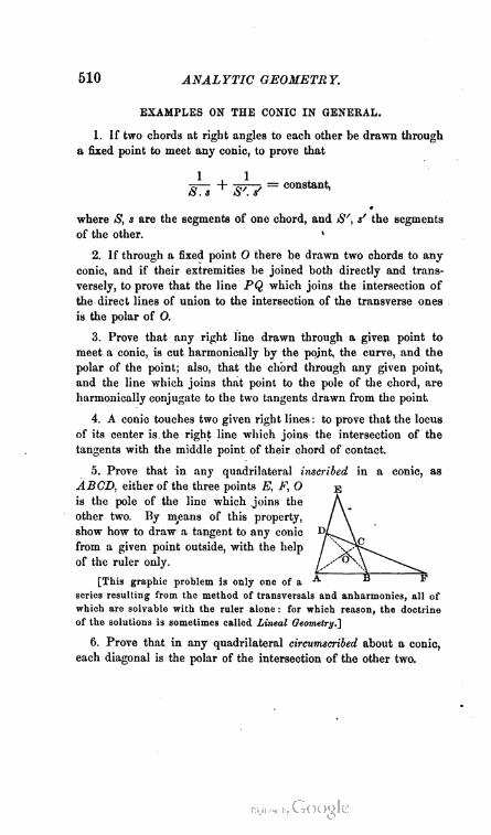
510 ANALYTIC GEOMETRY.
EXAMPLES ON THE CONIC IN GENERAL.
1. If two chords at right angles to each other be drawn through
a fixed point to meet any conic, to prove that
ks + sr? = con8tant'
where S, s are the segments of one chord, and iS", s' the segments
of the other. '
2. If through a fixed point O there be drawn two chords to any
conic, and if their extremities be joined both directly and trans
versely, to prove that the line PQ which joins the intersection of
the direct lines of union to the intersection of the transverse ones
is the polar of O.
3. Prove that any right line drawn through a given point to
meet a conic, is cut harmonically by the pojnt, the curve, and the
polar of the point; also, that the chord through any given point,
and the line which joins that point to the pole of the chord, are
harmonically conjugate to the two tangents drawn from the point.
4. A conic touches two given right lines : to prove that the locus
of its center is the right line which joins the intersection of the
tangents with the middle point of their chord of contact.
5. Prove that in any quadrilateral inscribed in a conic, as
ABCD, either of the three points E, F, O
is the pole of the line which .joins the
other two. By means of this property,
show how to draw a tangent to any conic
from a given point outside, with the help
of the ruler only.
[This graphic problem is only one of a
series resulting from the method of transversals and anharmonics, all of
which are solvable with the ruler alone : for which reason, the doctrine
of the solutions is sometimes called Lineal Geometry.']
6. Prove that in any quadrilateral circumscribed about a conic,
each diagonal is the polar of the intersection of the other two.

BOOK SECOND:
CO ORDINATES IN SPACE.
An. Ge. 46. (511)


CO-ORDINATES IN SPACE.
674. In removing, at this point in our investigations,
the restriction which has confined loci to a given plane,
we shall only enter upon the consideration of the most
elementary parts of the Geometry of Three Dimensions.
That is, we shall only undertake to give the student a
clear general outline of the principles by which we rep
resent and discuss the surfaces of the First and Second
orders. In order to accomplish this, we must begin, as
in the case of the Geometry of Two Dimensions, by
explaining the conventions for representing a point in
space.
CHAPTER FIRST.
THE POINT.
675. About a century after the publication of Des
cartes' method of representing and discussing plane
curves, Clairaut extended the method to lines and
surfaces in space, by the following contrivance for
representing the position of any conceivable point in
space.
(513)
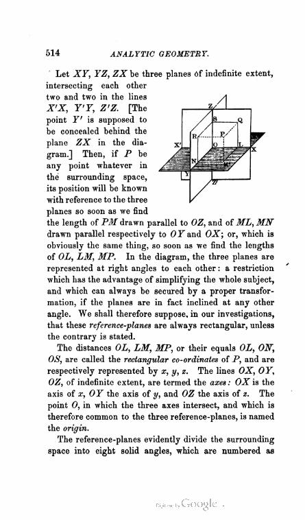
514 ANALYTIC GEOMETRY.
Let XY, YZ, ZX be three planes 6f indefinite extent,
intersecting each other
two and two in the lines
X'X, Y'Y, Z'Z. [The
point Y' is supposed to
be concealed behind the
plane ZX in the dia
gram.] Then, if P be
any point whatever in
the surrounding space,
its position will be known
with reference to the three
planes so soon as we find
the length of PM drawn parallel to OZ, and of ML, MN
drawn parallel respectively to Ol^and OX; or, which is
obviously the same thing, so soon as we find the lengths
of OL, LM, MP. In the diagram, the three planes are
represented at right angles to each other : a restriction
which has the advantage of simplifying the whole subject,
and which can always be secured by a proper transfor
mation, if the planes are in fact inclined at any other
angle. We shall therefore suppose, in our investigations,
that these reference-planes are always rectangular, unless
the contrary is stated.
The distances OL, LM, MP, or their equals OL, ON,
OS, are called the rectangular co-ordinates of P, and are
respectively represented by x, y, z. The lines OX, OY,
OZ, of indefinite extent, are termed the axes : OX is the
axis of x, OY the axis of y, and OZ the axis of z. The
point 0, in which the three axes intersect, and 'which is
therefore common to the three reference-planes, is named
the origin.
The reference-planes evidently divide the surrounding
space into eight solid angles, which are numbered as
RECTANGULAR CO-ORDINATES IN SPACE. 515
follows: Z-XOY is the first angle; Z-YOX', the
second; Z-X'OY', the third; and Z-Y'OX, the fourth.
Similarly, Z'-XOY is the fifth angle; Z'-FOX', the
si^A; Z'-X'OY', the gewratfA; and Z'-F'OX, the
eighth.
By affecting the co-ordinates x, y, z with the proper
sign, we represent a point in either of the eight angles.
Thus,
First angle : x = + a,y = + b, z = + c;
Second " x — — aiy =
+ b, z + c;
Third " x = — fit,y =
-h, 2 = + c;
Fourth " x = + a,y =
-b, 2 = + c;
Fifth " x = + a,y = + b, Z = — c;
Sixth " x = — ai y = + b, Z = — e;
Seventh " x = — a->y =
~b, Z = — c;
Eighth " X = + a,y =
~b, Z = — c.
The student will observe that the positive x lies to the
right of the first vertical plane YZ, and the negative x
to the left of that plane ; the positive y, in front of the
second vertical plane ZX, and the negative y in the rear
of that plane; the positive z, above the horizontal plane
XY, and the negative z below that plane.
Corollary 1.—For any point in the plane YZ, we shall
evidently have
x = 0 (1),
while y and z are indeterminate. Equation (1) is there
fore the equation to the first vertical reference-plane.
For any point in the plane ZX, we shall have
y = o (2),
while z and x are indeterminate. Hence, (2) is the
equation to the second vertical reference-plane.
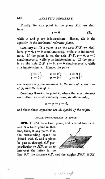
516 ANALYTIC GEOMETRY.
Finally, for any point in the plane XY, we shall
have
z = 0 (3),
while x and y are indeterminate. Hence, (3) is the
equation to the horizontal reference-plane.
Corollary 2.—If a point is on the axis X'X, we shall
have y = 0, z = 0 simultaneously, while x is indetermi
nate. If the point is on the axis Y'Y, 2 = 0, x = 0
simultaneously, while y is indeterminate. If the point
is on the axis Z'Z, x=0, y = 0 simultaneously, while
z is indeterminate. Hence, the pairs
y = 0) 2=0) X = 0)
z =0/' z=0j y = 0j'
are respectively the equations to the axis of x, the axis
of y, and the axis of %.
Corollary 3.—At the point 0, where the axes intersect
each other, we shall evidently have, simultaneously,
x — y = z = 0,
and these three equations are the symbol of the origin.
POLAR CO-ORDINATES IN SPACE.
676. If MN be a fixed plane, OX a fixed line in it,
and O a fixed point in that
line, then, if any point P in
the surrounding space be
joined with O, and a plane
be passed through OP per
pendicular to MN, so as to
intersect the latter in the
line OR, the distance OP, and the angles POB, BOX,

POLAR CO-ORDINATES IN SPACE. 517
are called the polar co-ordinates of the point I*. The
distance OP is called the radius vector, and is repre
sented by the letter p; the angles POR, BOX are
termed the vectorial angles, and are designated respect
ively by <p and 0, as in the diagram.
MN is called the initial plane, OX the initial line,
and 0 the pole. Instead of the angle <p, its complement
is sometimes used, designated by y.
By inspecting the diagram, it will be evident that we
may use
? = 0 (1)
as the equation to the initial plane,
<p = d = 0
as the equations to the initial line, and
p = 0 (3)
as the equation to the pole.
(2)
THE DOCTRINE OP PROJECTIONS.
Definitions.—The point in which a line in space
pierces a given plane, is called the trace of the line upon
the plane. Similarly, the line in which a surface cuts a
given plane, is termed the trace of the surface upon the
plane. In particular, the trace of one plane upon an
other, is the right line in which the former intersects the
latter.
If a perpendicular be let fall from any point to a
given plane, the trace of the perpendicular upon the
plane is called the orthogonal projection of the point on
the plane. When we use the term projection in what
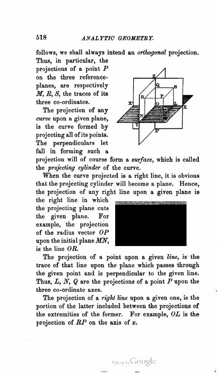
518 ANALYTIC GEOMETRY.
A
Q s
o ! L
follows, we shall always intend an orthogonal projection.
Thus, in particular, the
projections of a point P
on the three reference-
planes, are respectively
M, R, S, the traces of its
three co-ordinates.
The projection of any
curve upon a given plane,
is the curve formed by
projecting all of its points.
The perpendiculars let
fall in forming such a
projection will of course form a surface, which is called
the projecting cylinder of the curve.
When the curve projected is a right line, it is obvious
that the projecting cylinder will become a plane. Hence,
the projection of any right line upon a given plane is
the right line in which
the projecting plane cuts
the given plane. For
example, the projection
of the radius vector OP
upon the initial plane MN,
is the line OR.
The projection of a point upon a given line, is the
trace of that line upon the plane which passes through
the given point and is perpendicular to the given line.
Thus, L, JV, Q are the projections of a point P upon the
three co-ordinate axes.
The projection of a right line upon a given one, is the
portion of the latter included between the projections of
the extremities of the former. For example, OL is the
projection of RP on the axis of x.
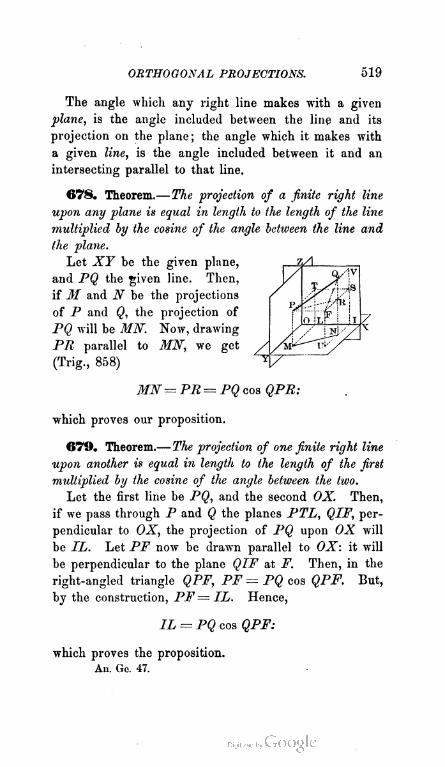
ORTHOGONAL PROJECTIONS. 519
The angle which any right line makes with a given
plane, is the angle included between the line and its
projection on the plane; the angle which it makes with
a given line, is the angle included between it and an
intersecting parallel to that line.
678. Theorem.—The projection of a finite right line
upon any plane is equal in length to the length of the line
multiplied by the cosine of the angle between the line and
the plane.
Let XY be the given plane,
and PQ the given line. Then,
if M and N be the projections
of P and Q, the projection of
PQ will be MN. Now, drawing
PR parallel to MN, we get
(Trig., 858)
MN=,PR= PQ cos QPR:
which proves our proposition.
679. Theorem.—The projection of one finite right line
upon another is equal in length to the length of the first
multiplied by the cosine of the angle between the two.
Let the first line be PQ, and the second OX. Then,
if we pass through P and Q the planes PTL, QIF, per
pendicular to OX, the projection of PQ upon OX will
be IL. Let PF now be drawn parallel to OX: it will
be perpendicular to the plane QIF at F. Then, in the
right-angled triangle QPF, PF = PQ cos QPF. But,
by the construction, PF= IL. Hence,
IL = PQ cos QPF:
which proves the proposition.
An. Go. 47.

520 ANALYTIC GEOMETRY.
680. Theorem.—In any series of points, ihe projection
(on a given line) of the line which joins the first and last,
is equal to the sum of the projections of the lines which join
the points two and two.
The points may be so situated that their projections on
the given line advance successively from the first to the
last : in which case the theorem is an obvious consequence
of the sixth definition in Art. 677. Or they may be so
placed that the projections of some fall on the given line
behind those of the next preceding points : in which case
we still obtain the theorem, if we consider the line which
joins such a point to its predecessor as forming a negative
projection, and understand the sum mentioned above as
algebraic.
Corollary.—The projection of the radius vector of any
point, is equal to the sum of the projections of the co
ordinates of the point.
For the points 0, L, M, P (see diagram, Art. 675)
may of course be considered as a series coming under
the above theorem.
DISTANCE BETWEEN TWO POINTS IN SPACE.
681. Let P and Q be the two points, projected re
spectively at 31, R, S and
N, T, V. Through P, pass a
plane JiPF, parallel to the ref
erence-plane XY; and letPML
be the projecting plane of MP,
and QNE of NQ. Then, in the
right-angled triangle QPF, we
shall have
PQ? = QF* + PF*
DIRECTION-COSINES OF A LINE. 521
But, by the construction of the figure, PF=MN; hence,
from the right-angled triangle MGN,
PF2 = NO* + MG2 (2).
Substituting in (1), we obtain
PQ2 = NG2 + MG2 + QF2.
Hence, if the co-ordinates of P be xf, y', z', and those
of Q be x", y", z", while d represents the distance PQ,
we have
g* = (x" — x*y + (y" — y'f + (z" — zj.
Corollary.—For the distance from the origin to any
point xy in space, we therefore have (Art. 675, Cor. 3)
8* = x2 + f + z2-
683. The last result may be interpreted thus: The
square on the radius vector of any point is equal to the
sum of the squares on the co-ordinates of the point.
This theorem leads to a remarkable relation among the
so-called direction-cosines of a right line, that is, the co
sines of the three angles which the line makes with the
three co-ordinate axes. Let the angle made with the
axis of x be «, that made with the axis of y be /9, and
that made with the axis of z be y. Then, supposing a
parallel to the given line to be drawn through the origin,
the co-ordinates of any point xyz on this parallel will be
the projections of its radius vector on the axes, and we
shall have (Art. 679)
x = p cos a, y — p cos /?, z = p cos y.
Squaring and adding these equations, and observing that
p2 = x2 -j- y2 -j- z2, we get, for the relation mentioned,
cos2 a + cos2 ft + cos2 y = 1.
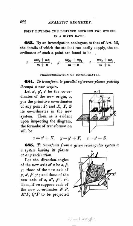
522 ANALYTIC GEOMETRY.
POINT DIVIDING THE DISTANCE BETWEEN TWO OTHERS
IN A GIVEN RATIO.
683. By an investigation analogous to that of Art. 52,
the details of which the student can easily supply, the co
ordinates of such a point are found to be
mx2 + nxx my., + nyt mz., + nzxX m + n ' y m + n ' Z m + n
TRANSFORMATION OF CO-ORDINATES.
684. To transform to parallel reference-planes passing
through a new origin.
Let x', y', z' be the co-or
dinates of the new origin, x,
y, z the primitive co-ordinates
of any point P, and X, Y, Z
its co-ordinates in the new
system. Then, as is evident
upon inspecting the diagram,
the formulae of transformation
will be
X = x' + X, y = y' + Y, z=z> + Z.
685. To transform from a given rectangular system to
a system having its planes
at any inclination.
Let the direction-angles
of the new axis of x be a, ft,
y, those of the new axis of
y, a', ft', f ; and those of the
new axis of z, a", ft", y".
Then, if we suppose each of
the new co-ordinates N'P,
M'P, Q'P to be projected

TRANSFORMATION OF CO-ORDINATES. 523
on one of the old axes, the sum of the three projections
(Art. 680, Cor.) will in each case be equal to the projec
tion of the radius vector OP. But the projection of OP
on OX will be equal to the old x of P; its projection on
OY, to the old y; and its projection on OZ, to the old z.
Hence, (Art. 679,)
x — X cos a + Y cos a' -\- Z cos a",
y = Xcos ,3 + Fcos ? + Z cos 0",
z — X cos y + Fcos f + Z cos r",
are the required formulae of transformation.
Remark.—It must be borne in mind, in using these
formulae, that the direction-cosines of the new axes are
subject to the conditions (Art. 682)
cos2 a + cos2 /? + cos2 y = 1,
cos2 a' + cos2 ft + cos2 f = 1,
cos2 a" + cos2/?" + cos2 f — 1.
686. To transform from a planar to a polar system
in space.
Let the planar system be rectangular. Then, the co
ordinates of any point P in the
two systems being related as in
the diagram, it is evident that
we shall have
x — p cos (f cos 0,
y = p cos <p sin 0,
z — p sin ip.
From these equations we can evidently also find p,<p,d
in terms of x, y, z.

524 ANALYTIC GEOMETRY.
Remark.—To combine a change of origin with this
transformation or that of the preceding article, we have
merely to add the co-ordinates x' , y', z' of the new origin
to the values found for x, y, and z.
GENERAL PRINCIPLES OF INTERPRETATION.
687. These follow from the convention of co-ordinates
in space in much the same manner as the principles of
Plane Analytic Geometry followed from the convention
of plane co-ordinates. We may therefore state them
without further argument, as follows:
I. Any single equation in space-coordinates represents
a surface.
To hold with full generality, this statement must be
understood to include (in addition to surfaces in the
ordinary sense) imaginary surfaces, surfaces at infinity,
surfaces that have degenerated into lines or points, and
surfaces combined in groups.
II. Two simultaneous equations in space-coordinates
represent a line of section betiveen two surfaces.
This principle is also to be taken with restrictions
corresponding to those above stated.
III. Three simultaneous equations in space-coordinates
represent mnp determinate points.
These are the points of intersection of three surfaces,
supposed to be of the mth, nth, and pth order respectively.
IV. An equation which lacks the absolute term, repre
sents a surface passing through the origin.
V. Transformation of co-ordinates in space does not
alter the degree of a given equation, nor affect the form
of its locus in any way.
\
THE PLANE. 525
CHAPTER SECOND.
LOCUS OF THE FIRST ORDER IN SPACE.
688. Form of the IiOcus.—The general equation of
the first degree in three variables, may be written
Ax +By + Cz + D = 0 (1),
where A, B, C, D are any four constants whatever.
Transforming (1) to parallel axes passing through a
new origin x'y', we get (Art. 684)
Ax + By+Cz + (Ax' + By' + Cz' + D) =0.
Hence, if we suppose the new origin to be any fixed
point in the locus of (1), the new absolute term will
vanish, and our equation will take the form
Ax + By + Cz = 0 (2).
If we now change the directions of the reference-
planes (Art. 685), we shall get, after expanding and
collecting terms,
(A cos a + B cos /? -f G cos y ) x \
+ (A cos a' + B cos ji' + Ccos f ) y > = 0.
+ (A cos a" + B cos ft" + Ccos /') z J
Hence, if Ave can take the new reference-planes so as to
give the new axis of x and the new axis of y such
directions that
A cos a + B cos /9 + 0 cos y = 0
= A cos a' + B cos /?' + C cos y' (q),
we shall reduce our equation to the simple form
z = 0 (3).

526 ANALYTW GEOMETR Y.
Now, obviously, the transformation from (1) to (2) is
always possible ; and that we can always effect the
transformation from (2) to (3) will readily appear.
For we can leave the primitive vertical reference-planes
unchanged, obtaining our new system by merely revolv
ing the primitive horizontal plane about the origin: in
which case, we shall have
a = 90° — r, /3=0; «' = 0, /3'=90° — f ;
and the conditions at (q), upon which the transformation
we are now considering depends, will become /
QA sin y -f Ccos y = 0 i. e. tan y = ,
cB sin yr -f C cos f = 0 i. e. tan y' = — ^- :
suppositions compatible with any real values of A, B, 0.
We conclude, then, that by a proper transformation
of co-ordinates we can always reduce the general equa
tion of the first degree to the form
z = 0.
But this [Art. 675, Cor. 1, (3)] denotes the new refer
ence-plane XY. Hence, (Art. 687, V,) The locus of the
First order in space is the Plane; or, as we may otherwise *
state our result, Every equation of the first degree in space
represents a plane.
THE PLANE UNDER GENERAL CONDITIONS.
689. General Form of the Equation to the
Plane.—From what has just been shown, we learn
that
Ax + By + Cz + D = 0
is the Equation to any Plane.
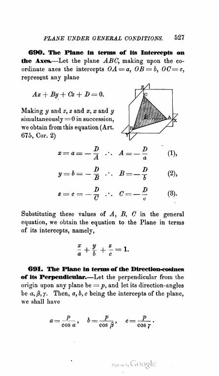
PLANE UNDER GENERAL CONDITIONS. 527
GOO. The Plane in terms of its Intercepts on
the Axes.—Let the plane ABC, making upon the co
ordinate axes the intercepts OA = a, OB = b, OC=c,
represent any plane
Z/
Ax + By + Cz + B = Q.
Making y and z, z and x, x and y
simultaneously = 0 in succession,
we obtain from this equation (Art. A
675, Cor. 2) ^
x = a = —B
D
B
z = c = —D
G
B = .
0 = -
D
b
(1) ,
(2) ,
(3) .
generalSubstituting these values of A, B, Cm the
equation, we obtain the equation to the Plane in terms
of its intercepts, namely,
a o c
601. The Plane in terms of the Direction-cosines
of its Perpendicular.—Let the perpendicular from the
origin upon any plane be =p, and let its direction-angles
be a, /9, y. Then, a, b, c being the intercepts of the plane,
we shall have
528 ANALYTIC GEOMETRY.
Substituting these values in the equation of the preced
ing article, ive obtain
x cos a-\-y cos ft + z cos y=p,
the equation to the Plane in the terms now required.
692. Reduction of the General Equation to the
form last found.—We may suppose the reduction to be
effected by dividing the general equation
Ax + By + Cz + D= 0
throughout by some quantity Q. If so, we shall have
A — Q cos a, B = Q cos ft, C—Q cos y : whence
Q- (cos2 a + cos2 ft + cos2 y) = A2 + B2 + C2.
Now (Art. 682), cos2 a + cos2 ft + cos2 y = 1. Hence,
Q = VA2 + B' + (J2; and we learn that
cos a ---
V(A2 + B*+ C2)'
a- Bcoa^-y{Ar+B^TO^y
0cos y =
V(Al + Bi + o2) '
and that, for the perpendicular from the origin upon a
plane given by the general equation, we have
V(A2 + B2+ C2) '
By always taking the radical Q with that sign which
will render p positive, the resulting signs of cos a, cos ft,

PLANE UNDER SPECIAL CONDITIONS. 529
cos y will indicate whether the direction-angles of the
perpendicular are acute or obtuse.
THE PLANE UNDER SPECIAL CONDITIONS.
693. Equation to a Plane passing through Three
Fixed Points.—By a process exactly analogous to that
of Art. 95, this is found to be
[y'(*"-it"')+y'(."'-«')+y"'(«'-»")]*') f (y"*'"-y'v )x'
+ [x'(x"-x"')+*"{x"'—a;')+«"'(x/—x")]y [ = ] + (/"»' — y' z'")x"
+ W-j"')+x"(j"'-y')+*"'(y'-y")]«) (.+ (✓ )*"',
in which a/y'z', x"y"z", x"'y"'z"' are the three points
which determine the plane.
G94. Angle between two Planes.—This is evidently
equal, or else supplemental, to the angle between the
perpendiculars thrown upon the planes from the origin.
Now, if p, p' be the lengths of these perpendiculars,
a, /?, y an(i a'i ft'■> Y their direction-angles, and o the
distance between the points xyz, x'y'z' in which they
pierce their respective planes, we shall have (Art. 681)
p2-\-p'2— 2pp' cosf = 82~(x— a/)2+ {y—y')2-\- (z— z')2,
where <p = the angle between the planes or their per
pendiculars. But (Art. G81, Cor.) p2 = x2 + y2 -f z2,
and p'2 — a/2 + y'2 -\- z'2. Hence, after obvious reduc
tions,
pp' cos <p = xx1 + yy' + zz' ;
or, since x=pcosa, y=pcosfl, z=p cosy; x'=p' cos a',
y' = p' cos /3', z' = p' cos y',
cos ^ = cos a cos «'+ cos /? cos /?'-)- cos f cos -f (A)-
Here it becomes evident, upon a moment's reflection,
that the direction-angles y and y' are respectively equal

530 ANALYTIC GEOMETRY.
to the angles which the two planes make with the hori
zontal reference-plane ; that a and a' are respectively
equal to those made with the first vertical plane ; and
that /? and ;5' are respectively equal to those made with
the second vertical plane. Calling these new angles
£ and f', u and u', £ and we have, then, as the ex
pression for the angle between two planes in terms of their
inclinations to the reference-planes,
cos tp = cos ? cos f' -f- cos y cos u' + cos £ cos £' (1).
Replacing the cosines in (1) by their values from Art.
692, namely,
c cj/^2 + £2 + 6*) ' • + + C'2) '
A A'COS V = ,, A, ,—777—■—-v.,-7 , COS t/=
+ 2? + C") ' V(A'*+ V") '
B „ B'COS C = , , ... ,—777——777T , COS C =y + £2 + c) ' v' (4/a + Bn + tf"*) '
we obtain, as the expression for the angle between two
planes in terms of the co-efficients of their equations,
_ AA'+BB'+GC m
Corollary 1.—The two planes will be parallel if <p — 0 ;
that is, if cos <p = 1. As the condition of parallelism,
then, the terms of the second member of (2) must be
equal ; or, after squaring and transposing,
(AB'—A'B)1 + (BO' —B'CY + (CA'—C'A)2= 0 :
a condition which can only be satisfied by having simul
taneously
A b^_d o^__c
B1 ~B' C ~ 0' A' ~ A'

PARALLELISM AND PERPENDICULARITY. 531
Corollary 2.—If the two planes are perpendicular to
each other, we shall have cos f = 0 : whence, as the
condition of perpendicularity,
AA! + BB' + CO' = 0.
695. Equation to a Plane parallel to a given
one.—From the condition reached in the first corollary
to the preceding article, it is evident that this can finally
be written in the form
Ax'+By + Cz + iy=0,
A, B, C being the co-efficients of x, y, z in the equation
to the given plane. We learn, then, that the equations
to parallel planes differ only in their constant terms.
Corollary.—The equations to planes parallel respect
ively to the three reference-planes, will be
z = constant, x = constant, y = constant.
■
696. Equation to a Plane perpendicular to a
given one.—If A'x + B'y -j- C'z + V = 0 be the given
plane, we may write the required equation in either of
the forms
Px — By—Cz — D = Q (1),
Ax-Qy+Cz + D = 0 (2),
Ax + By—Rz+D = 0 (3),
by merely making, in accordance with Art. 694, Cor. 2,
BB'+CC n CC'+AA' _ AA'+BB'
r — ' V~ B' ' C>
Corollary.—In particular, the equations to planes per
pendicular to the reference-planes will assume the forms
Ax+By +I)= 0, By +Cz+D=0, Cz+Ax+D=0.
532 ANALYTIC GEOMETRY.
For (Art. 675, Cor. 1) Ii must vanish for the horizontal
reference-plane, P for the first vertical, and Q for the
second.
G97« ILength of the Perpendicular from a Fixed
Point to a Given Plane.—Let the fixed point be xyz,
and the given plane x cos a + y cos /? + z cos y —p = 0.
If we produce the perpendicular p, and then project upon
it the radius vector of xyz, it is evident that the required
perpendicular will be equal to the difference between this
projection and p. Hence, (Art. 680, Cor.,) we have
P= ± (zcos a + y cos/9 + zeosy —p),
the upper or lower sign being used according as the
given point and the origin lie on opposite sides of the
given plane, or on the same side.
Corollary 1.—For the perpendicular from xyz to the
plane Ax + By + Cz + D = 0, we have (Art. 692)
Ax + By+Cz + B
^(A' + B' + C2) '
Corollary 2.—Since we have agreed to consider the
perpendicular from the origin upon any plane as positive
in all cases, consistency requires that perpendiculars
dropped upon a plane from any point on the same side
of it as the origin, shall be reckoned positive; and those
dropped from the opposite side, negative.
698. Equation to a Plane passing through the
Common Section of two given ones.—By reasoning
similar to that of Arts. 107, 108, it is evident that this
may be written
(Ax + By + Cz + B) + k (A'x + B'y + O 'z + &) = 0 ;
\

INTERSECTIONS OF PLANES. 533
or, by adopting abridgments similar to those used in
Plane Geometry,
P+kP'=Q.
Corollary.—Analogy leads at once to the conclusion,
that an equation of the form
IP + mP' + nP" = 0,
in which I, m, n are arbitrary constants, denotes a plane
passing through the point in which the three planes P,
P', P" intersect.
699. Equation to the Plane bisecting the angle
between two given ones.—The reasoning of Art. 109
applies here, and the required equation (Art. 692) is
Q'P±QP' = 0 (1),
or, if the equations to the given planes are already re
duced to terms of their direction-cosines,
«±/? = 0 (2),
the upper sign denoting the external bisector, and the
lower the internal one.
700. Condition that Four Points shall lie on
one Plane.—The fourth point must of course satisfy the
equation to the plane of the other three, and the required
condition is therefore obtained by putting xIvy™zlv instead
of xyz in the equation of Art. 693.
701. Condition that Three Planes shall pass
through one Right Line.—The equation to the third
plane must take the form (Art. 698) of the equation to

534 ANALYTIC GEOMETRY.
a plane passing through the common section of the other
two. There must, then, be some constant — n, such that
— nP" = lP + mP'.
Hence, the required condition is»
IP+mP' + nP"=0.
In other words, Three planes pass through one right line
whenever their equations, upon being multiplied by three
suitable constants and added together, vanish identically.
702. Condition that Four Planes shall meet in
One Point.—By applying the reasoning of the preceding
article to the result of the corollary to Art. 698, we learn
that this condition may be written
IP + mP' + nP" + rP1" = 0 ;
or, if the equations to the planes be in terms of their
direction-cosines,
la + ?»/3 + ny + rd = 0.
Hence, Four planes pass through one point tvhenever their
equations, upon being multiplied by four suitable constants
and added together, vanish identically.
QUADRIPLANAR CO-ORDINATES.
703. The condition of the preceding article subjects
its constants I, m, n, r to certain restrictions, consistent
with the identical vanishing of the function
la + mfl + ny + rd.
But if we now free these constants from this condition
for the converging of four planes, making them abso-
X

RIGHT LINE IN SPACE. 535
Iutely arbitrary, we learn, by reasoning entirely analo
gous to that of Arts. 208—217, that if a = 0, = 0,
y = 0, d = 0 be the equations to any four planes forming
a tetrahedron, the equation
la + mft -j- + rd = 0
is a general symbol for any plane in space.
We thus arrive at what may be called a system of
quadriplanar co-ordinates, analogous to the trilinear
system of Plane Geometry.
LINEAR LOCI IN SPACE.
704. By II of Art. 687, it appears that all lines in
space, whether right or curved, are to be solved as the
common sections of two surfaces, and hence must be rep
resented by two simultaneous equations in three variables.
In particular, the Right Line in Space, which is the only
line we shall have room to consider, must be treated as
the common section of two planes.
705. Equations to the Right Line in Space.—We
might represent this line by the two general equations
Ax + By + Cz-\- D=0, A'x + B'y+C'z + & = (),
but it is far more convenient to denote it by the simul
taneous equations of its two projecting planes (Art. 677),
in accordance with the method by which all curves in
space are usually represented by means of their " pro
jecting cylinders."
In pursuance of this method, then, the equations to
the Right Line projected upon the two vertical reference-
planes, will be of the form (Art. 696, Cor.)
By + Cz + D= 0, Nz + Mx + L = 0.
An. Ge. 48.

536 ANALYTIC GEOMETRY.
Now it is noticeable, that, while these equations taken
together involve three variables, each of them taken sep
arately involves but two. The first, interpreted as an
equation in two variables, denotes a right line in the
first vertical plane; the second, similarly interpreted,
denotes a right line in the second vertical plane. But
these lines, by the principle of the corollary to Art. 696,
must also lie in the two planes which the equations denote
when interpreted in space : hence, they are the common
sections of these planes and the vertical planes of refer
ence ; or, in other words, they are the projections of the
right line represented by the simultaneous equations
By + Cz + D = 0, Nz + 3Ix + L = 0, upon the two
vertical reference-planes.
We see, then, that we may either regard the two
determining equations of the Right Line as the space-
equations to its two projecting planes, or as the plane-
equations to its two projections. It is customary to
interpret them in the latter way, and as each involves
two, and only two, arbitrary constants, to write them
x — mz + a, y = nz-\-b.
Thus the axis of z is made their common axis of abscissas,
and the constants in, a, n, b take meaning as follows :
m— the tangent of the angle which the projection
on the second vertical plane makes with the
axis of z.
a — the intercept which the same projection forms
on the axis of x.
n = the tangent of the angle which the projection
on the first vertical plane makes with the
axis of z.
b — the intercept which this projection forms on
the axis of y.

RIGHT LINE IN SPACE. 537
We learn, then, that the position and direction of a right
line in space, depend upon the magnitudes and signs of
four arbitrary constants.
706. Symmetrical Equations to the Right Line
in Space.—Let the line pass through an arbitrary point
x'y'z', and let its direction-angles be «, /?, y.
Then, if I — the distance from x'y'z' to any point xyz
of the line, the projections of I upon the three co-ordi
nate axes (Art. 679) will be I cos a, I cos /9, I cos y. But
by definition (Art. 677) these projections are respectively
equal to x — x1, y — y', z — z'. Hence,
I cos a = x — x', I cos /? = y— y', I cos y = z — z' :
whence, solving for I and equating the three results,
x — x' y — if z — z' ,
cos a cos /? cos y
which are the symmetrical equations sought.
7©7. To find the Direction-cosines of a Right
lane given hy its Projections.—The direction-cosines
of any right line are of course the same as those of its
parallel through the origin. Let the projections of such
a parallel be
xyz
I m n
Then, if p be the radius vector of any point xyz on the
parallel, we shall have (Art. 681, Cor.)
p" = x2 + y" +• z2,
and, from the above equations of projection,
mx nxy = T> Z = T-
538 ANALYTIC GEOMETRY.
Solving the last three equations for x, y, z, we obtain
lp mpX = y {F + m2 + n2) ' V = i/(P + m2 + n2) '
npZ ~ VW + + n2) '
But, by the doctrine of projections,
x = p cos a, y = p cos /?, z — p cos y.
Substituting, and dividing through by p,
I a m003 a = /in i T1 Y\ ' cos P — 77m i 2~i 2\ »
w
Corollary.—To find the direction-cosines of a line
whose projections are given in any form whatever,
throw its equations into the form
x — x' y — y' _ z — / .
I m n
when the required functions will be I, m, n, each divided
by Vl1 + m2 + n2.
708. Angle between two Ones in Space.—The
angle 6 between two right lines in space is obviously
equal to that between their respective parallels through
the origin. Hence, by formula (a) of Art. 694,
cos 0 = cos a cos a' + cos /3 cos /?' + cos y cos y' (1) :
which expresses the angle between two right lines in terms
of their direction-cosines.

PLANE ANGLES IN SPACE. 539
Substituting for cos «, cos a', etc., from the preceding
article, we get
„ IV + mm' 4- nn' /n.cos 0 — ' (2) :
^{l2 + m1 + n2) {I'2 + m'2 4- n'2) v ;
which expresses the angle between two rigid lines in terms
of their projections.
Corollary 1.—The condition that two right lines in
space shall be parallel, derived from (1), is
cos a cos a' + cos /9 cos /?' + cos y cos f = 1 (1),
or, derived from (2) by steps analogous to those in the
first corollary of Art. 694,
V I , m! m t n' n
m! m ' n' n ' V I
Corollary 2.—The condition that two right lines in
space shall be perpendicular to each other, derived from
(1), is
cos a cos a! + cos /9 cos /3' + cos y cos y' — 0 (1),
or, derived from (2),
IV + mm' + nn' = 0 (2).
709. Equation to a Right Line perpendicular
to a given Plane.—If Ax + By + Cz + D= 0 be the
given plane, the required equation may be written
x — & _y — b z — c
For we may suppose the perpendicular to pass through
any fixed point abc; and, by Art. 692, its direction-
cosines must be proportional to A, B, C.
710. Angle contained between a Right Line
and a Plane.—This being the complement of the angle

540 ANALYTIC GEOMETRY.
contained between the given line and a perpendicular
to the plane, if the given line be
x— a/ y — y' z— z'
I m n '
we have, by comparing Arts. 708, 709,
• ff— Al + Bm+ On8m ~~ y{A1 + B2 + G'2) (I2 + m2+ n2) "
Corollary.—The condition that a right line shall be
parallel to a given plane, is
Al + Bm +On = 0.
711. Condition that a Right Line shall lie
wholly in a given Plane.—If a right line lies wholly
in a given plane, the z co-ordinate resulting from an
elimination between the equation to the plane and those
of the line must of course be indeterminate. Hence, if
the plane be Ax + By + Cz + B — 0, and the line
(x = mz -{-a, y = nz -f- b), so that we have by elimi
nation A {mz + a) + B (nz + b) + Cz + B — 0, or
__Aa + Bb + B
2~ Am + Bn+ C"
we must have, as the condition required, the simultaneous
relations
Am + Bn + 0= Aa + Bb + B — 0.
Remark.—This result is corroborated by the fact, that
the vanishing of the numerator of z indicates that the
point (a, b, 0), in which the line pierces the horizontal
reference-plane, is in the given plane ; while the vanish
ing of the denominator shows, by the corollary to the
RIGHT LINES MEETING IN SPACE. 541
previous article, that the line is parallel to the given
plane : two conditions which obviously place the line
wholly in that plane.
712. Condition that two Right Lines in Space
shall intersect.—Two right lines in space will not in
general intersect, because the four equations
x — mz + a, y = nz + b,
x = m'z + a', y = n'z + b',
being in general independent, are not compatible with
simultaneous values of the three variables x, y, z. If,
then, the two lines represented by these four equations
do intersect, one of the equations must be derivable from
the other three, and the condition of such a derivation
will be the required condition of intersection.
We form this condition, of course, by eliminating x, y, z
from the four equations. To do this, solve the first and
third, and also the second and fourth, for z, and equate
the two values thus found. The result is
m—m' a — a'
n — n' b — b'
EXAMPLES INVOLVING EQUATIONS OF THE FIRST DEGREE.
1. Show that, if L, M and N, R be the equations to two inter
secting right lines, they will be connected by some identical rela
tion
IL + mM+ nN+ rR = 0,
and that the plane of the two intersecting lines may be represented
by either of the equations
IL + mM^O, nN+rR=--0.
2. Find the equation to the plane which passes through the
lines
a; — a v — b z — c x — a v — b z — c

542 ANALYTIC GEOMETRY.
3. Find the equations to the traces of any given plane upon
the three reference-planes, and prove that if a right line be perpen
dicular to a given plane, its projections will be perpendicular to the
traces of the plane.
4. Find the equations to the three planes vrhich pass through
the traces of a given plane upon the reference-planes, and are each
perpendicular to the plane.
5. Find the equation to the plane which passes through a
given right line and makes a given angle with a given plane.
6. If (</, /?' Y), (a", /3", y") be the direction-angles of two
right lines, prove that the direction-cosines of the external bisector
of the angle between them, are proportional to
cos a' + cos a", cos j¥ -f cos /?", cos Y + cos Y',
and that those of the internal bisector are proportional to
cos a' — cos a", cos — cos /?", cos Y — cos Y'-
7. Three planes meet in one point, and through the common
section of each pair a plane is drawn perpendicular to the third :
prove that in general the planes thus drawn pass through one right
line.
8. Find the equation to a plane parallel to two given right lines,
and thence determine the shortest distance between the lines.
9. A plane passes through the origin : find the bisector of the
angle between its traces on two of the reference-planes.
10. Prove that the locus of the middle points of all right lines
parallel to a given plane, and terminated by two fixed right lines
which do not intersect, is a right line.
OHAPTEE THIRD.
LOCUS OF THE SECOND ORDER IN SPACE.
713. The general equation of the second degree in
three variables, which is the symbol of the space-locus
of the Second order, may be written
Ax2 + 2Hxy + By2 + 2Kyz + Ez2 + 2Lzx
+ 2Gx + 2Fy + 2Dz + C=0 (1),

SPACE-LOCUS OF THE SECOXD ORDER. 543
where A, B, E; H, K,L; C, D, F, G are any ten con
stants whatever.
Since we can divide this equation throughout by 0, it
appears that the number of independent constants is nine.
Hence, nine conditions are necessary and sufficient to
determine the locus. Thus we learn that, for example,
the space-locus of the Second order is a surface of such
a form that one, and but one, such surface can he passed
through any nine points which do not lie in the same plane.
The most general and complete criterion of the
form of any surface, is afforded by its curves of section
■with different planes. Let us apply this criterion to test
the figure of the surface denoted by (1).
If in (1) we make z = 0, that is, if we combine (1)
with the equation to the horizontal reference-plane, we
get
Ax2 + 2Hxy + By2 + 2Gx + 2Fy+ C= 0,
the general equation to the Conic. Hence, as we can
transform the reference-plane of XY to any plane that
we please, and as such a transformation will not affect
the degree of the equation of section just found, Every
plane section of a surface of the Second order is a conic.
Moreover, if we combine (1) with z = Jc, that is (Art.
695, Cor.), if wo intersect our locus by any plane parallel
to the plane of XY, we get
Ax2 + 2Hxy + Bf + 2G'x + 2F'y +C' = 0,
where G'=G + kL, F'=F+kK, C' =C+ 2kD+ k2K
Hence, (Art. 669,) since the co-efficients A, H, B remain
unchanged whatever be the value of h, The sections of a
surface of the Second order by parallel planes are similar
conies.
An. Ge. 49.
544 ANALYTIC GEOMETRY.
To denote, then, that the surface of the Second order
is represented by an equation of the second degree in
space, and that all its plane sections are curves of the
Second order, we shall henceforth call it the Quadric.
THE QUADRIC IN GENERAL.
715. To increase the clearness of our conception of
the quadric figure, we must now reduce the general
equation (1) to its simplest forms. We can effect this
reduction most rapidly, however, by taking out a few
leading properties of the surface, partly from the general
equation itself, and partly from the results of its first
transformations.
71C. Let us transform (1) to parallel axes through a
new origin x'y'z'. Since we merely have to write x + x'
for x, y -f- y' for y, and z + z' for z, it is easily seen that
the new equation will be
Ax2 + 2LTxy + By2 + 2Kyz + Ez2 + Lzx
+ 2G'x + 2F'y + 2D'z + C = 0 (2),
where C, the new absolute term, is the result of substi
tuting x'y'z' in (1), and in the new co-efficients of x, y, z
we have
G' = Ax' + Hy> + Lz' + G,
F' = ffx' + By' + Kz' + F,
D> = Lx' + Ky' + JEz' + A
these quantities being planar functions of the new origin.
It deserves especial notice, that G' (Alg., 411) is the
* For the discussion of Quadrics in complete detail, the reader is referred
to Salmon's Geometry of Three Dimensions, from which the investigations
of the following pages have in the main been reduced.
\

DISCRIMINANT OF THE QUADRIC. 545
derived polynomial (or derivative, as we shall call it for
brevity) of C with respect to x; that F' is the derivative
of C" with respect to y; and B', the derivative of C with
respect to z. Hence, if we write the original equation
(1) in the abbreviated form U = 0, we may use for the
four co-efficients C, G', F', If the convenient symbols
U' V U' U'
717. As we shall also find it convenient to employ
the so-called discriminant of the equation U — 0, and
several of its derivatives, we will determine their values
before advancing farther.
The discriminant of any function may be defined as
the result obtained by solving its several derivatives for
its variables, and then substituting the values of these
in the function itself. Accordingly, solving for x, y, z in
Ux = Ax + Hy + Lz + G = 0,
U„ = Hx + By +Kz+ F=0,
U, = Lx + Ky + Ez + D=0,
and then substituting in U, we get
ABCE+ 2ABFK+ 2BDGL + 2CHKL + 2EFGH
— ABB2—ACK~—AEF2—BCLi—BEGi— CEH2
+ K2G2 +L2F2+H2IP—2DFHL—2I)GHK—2FGKL.
This, then, is the discriminant of the given quadric Z7= 0,
and may be appropriately represented by A.
If we now denote the several derivatives of J, taken
with reference to G, F, B, C in succession, by 2g, 2f, 2d, c,
we shall have
g = BBL + EFH— BEG + GK2 — DHK— FKL,
f= ADK+ EGR — AEF+FL2 — BHL — GKL,
d = AFK+ BGL — ABB + BH2 — FHL — GHK,
c = ABE + 2HKL — AK2 - BL2 — EH2.

546 ANALYTIC GEOMETRY.
718. It will be convenient next to determine the
condition upon which the radius vector of the Quadric
will be bisected in the origin. To find this, throw the
general equation into the vectorial form, by writing
j> cos a for x, p cos /? for y, and p cos y for z, which we
may evidently do if a, fi, y are the direction-angles of
the radius vector. Equation (1) then becomes
{A cos2 a -f 2Hcos a cos (1 + B cos2 /?
+ 2Kcos p cos y + Ecos2 y + 2L cos y cos a) p2
+ 2(<?cosa + .Fcos/3+Dcos >-)/>+ C=0.
If the origin bisects the radius vector, this equation will
have its roots numerically equal with opposite signs.
Hence, the required condition of bisection is
G cos a + Fcos [i + D cos y — 0 ;
or, after multiplying through by p, and replacing the
corresponding x, y, z, we learn that all radii vectores
bisected in the origin must lie in the plane
Gx + Fy 4- Dz = 0.
719. If, then, in the equation to the Quadric we had
G, F, D all = 0, the condition of bisection would be
satisfied for all possible values of a, /9, y; or, in other
words, every right line drawn through the origin to meet
the quadric would be bisected in the origin, and the origin
would be a center of the quadric.
720. Resuming now our transformations of equation
(1), let us suppose the new origin x'y'z' to which (2) is
referred, to be a center. The new G, F, D will then
vanish, and we learn (Art. 716) that the center lies at
the intersection of the three planes *
ux = o, uv = o, uz = o.
QUADRICS CENTRAL AND NON-CENTRAL. 547
Solving these three equations, we obtain, as the co-ordi
nates of the center,
* = y' = t, z> = *,
c c c
where g, f, d, c have the values given in the table of
Art. 717.
The center, then, is a single determinate point, and
will be a finite real one if c is not zero, but not other
wise. Hence, Quadrics are either central or non-central,
and central quadrics have only one center.
721. By taking, then, the center for origin, the equa
tion to any central quadric may be written
Ax2+ 2Hxy +Bf+ 2Kyz +Uz2+ 2Lzx + C'= 0 (3),
where (Art. 716) by substituting the co-ordinates of the
center in V, we readily find
C'= G-c' ± H + Dd ± Cc = - ,
where G, F, D, C are -the co-efficients of the planar
terms of (1), and g, f, d, c, J have the meanings assigned
in Art. 717.
722. Let us next inquire into the form of the diame
tral surfaces of the Quadric.
A diametral surface of a given surface may be defined
as the locus of the middle points of chords drawn par
allel to a given right line. Suppose, then, that «, /?, y
are the direction-angles common to a system of chords
in a quadric, and let us remove the- origin of equation
(1) to any point on the locus of the middle points of the

548 ANALYTIC GEOMETRY.
system. By Art. 718, the new co-efficients G', F', If
must then fulfill the condition
G' cos « 4- F' cos /3 4- D' cos y = 0,
and the equation to the diametral surface of the Quadric
will therefore be (Art. 716)
Ux cos a 4- Uv cos /3 4- ZZ, cos ^ = 0.
This (Art. 698, Cor.) denotes a plane passing through
the intersection of the three planes Ux, Uv, Uz, namely
(Art. 720), through the center; and, as the direction-
angles a, ft, y are arbitrary, we have the theorem :
Every surface diametral to a quadric is a plane passing
through the center, and every plane passing through the
center of a quadric is a diametral plane.
It should be observed, of course, that this theorem
applies to the non-central quadrics only by regarding a
point infinitely distant from the origin as their center.
Such, indeed, is the fact indicated by the central co
ordinates (Art. 720) g : c, f :c, d : c, in which c — 0 for
the non-central quadrics. But if the diametral planes
pass through a common point at infinity, their several
common sections will meet in a point at infinity; in
other words, will be parallel. Hence, The diametral
planes of a non-central conic are parallel to a fixed
right line.
723. The diametral planes which bisect chords
parallel to the axis of x, the axis of y, and the axis
of z respectively, are found by successively supposing
/3 = r = 90°, r = a = 90°, a = /? = 90° in the equation
of the preceding article. They are therefore respectively

CONJUGATE PLANES AND DIAMETERS. 549
Ux — 0, Uy — 0, ZZ, = 0 ; or, writing the abbreviations
in full,
Ax + Hy + Lz + G = 0,
Hx + By + Kz+F= 0,
Zz -f Ky + Ez + D = 0.
For brevity, a diametral plane is said to be conjugate
to the direction of the chords which it bisects. Now the
condition that the plane Ux, which is conjugate to the
axis of x, may be parallel to the axis of y, according to
the corollary of Art. 696 is H = 0. But, obviously,
this is also the condition that the plane Uv, which is
conjugate to the axis of y, may be parallel to the axis
of x. Hence, as the co-ordinate axes may have any
direction, If a diametral plane conjugate to a given
direction be parallel to a given right line, the plane con
jugate to this line, will be parallel to the first direction.
724. If in our general equation (1) we had H, K, L
all — 0, the equations of the preceding article would be
reduced to
Ax+G = 0, By + F=Q, Ez + D = 0.
The diametral planes conjugate to the three axes would
thus (Art. 695, Cor.) become parallel to the reference-
planes; and, by the theorem last proved, each would be
conjugate to the common section of the other two.
Three diametral planes thus related are called conju
gate planes, and the three right lines in which they cut
each other two and two are called conjugate diameters.
Three diameters are therefore conjugate, when each is
conjugate to the plane of the other two.
We thus reach the important result, that whenever the

550 ANALYTIC GEOMETRY.
equation to a quadric lacks the co-efficients H, K, L, the
co-ordinate axes to which it is referred are parallel to a
set of conjugate diameters ; and, conversely, that by em
ploying axes parallel to a set of conjugates, we can always
cause these co-efficicnts to vanish from the equation to a
central quadric.
725. As the foregoing argument evidently does not
conflict with the supposition all along made, that the co
ordinate axes are rectangular, it follows that every central
quadric has one get of conjugate planes and diameters which
are at right angles to each other.
In fact, diametral planes perpendicular to the chords
which they bisect, or principal planes, as they are called,
exist in all quadrics whether central or not ; though the
triconjugate groups, of course, are peculiar to central
quadrics. For if we seek the condition that the plane
(Art. 722)
Ux cos a + Uy cos ft + Ut cos y = 0
may be perpendicular to its conjugate chords, the prin
ciple (Art. 709) that the direction-cosines of the chords
must be proportional to the co-efficients of the plane,
gives us, if we put k = the constant ratio between these
quantities,
A cos a + H cos ft + L cos y = k cos a,
H cos a -\- B cos ft -f- K cos y — k cos ft,
L cos a -j- jSTcos ft -f- E cos y = k cos y.
Eliminating cos a, cos ft, cos y from these equations, the
required condition is
THE PRINCIPAL PLANES. 551
¥— (A + B + E)k-
+(AB + BE+EA— H2 — K2 — L2)k — c=0,
where c has the same value as in Art. 717. Having
thus a cubic for determining the ratio k, we learn that
a quadric has in general three, and only three, principal
planes.
In the non-central quadrics however, since in them
(Art. 721) we have c = 0, one of the roots of this cubic
must be 0, and the equation to one of the principal planes
will therefore assume the form •
Ox -f- Oy + Oz + constant = 0.
In the non-central quadrics, therefore, by the analogy
of Art. 110, the third principal plane is situated at
infinity.
726. We are now prepared to put our general equa
tion into its simplest forms.
First, let us suppose that the derivative c is not zero.
From equation (3) in Art. 721, which is already referred
to the center as origin, we can at once proceed by taking
for new axes a set of conjugate diameters; and, as we
still adhere to rectangular co-ordinates, let these new
axes be conjugate to the principal planes. Then (Art.
724) the co-efficients H, K, L vanish from (3), and the
equation to any central quadric takes the form
A'x2 + By+E'z2+ C" = 0 (4).
Secondly, suppose that c is equal to zero. We can
not then arrive at the form (3) ; but, going back to (1),
we may first change the direction of the rectangular
axes, and then remove the origin. Now it can readily
552 ANALYTIC GEOMETRY.
be shown, that, in passing from one set of rectangular
axes to another, the new co-efficients of x2, y2, z2 (or A',
B', E') are the three roots of the cubic *
m3 — (A + B + E) u2
+ (AB +BE+EA—H2—K'—L2) w— e = 0.
* We append Salmon's proof of this, as it is remarkable for its brev
ity. See his Geometry of Three Dimensions, p. 50.
" Let us suppose that by using the most general transformation, which
is of the form «
x — \x + py + vz, y = Vx + n'y + v'z, z = \"x + p"y + v"z,
that Ax2 + 2Hxy + By2 + 2Kyz + Ez2 + 2Lzx
becomes A'x2 + 2H'~xy + B'y2 + 2Kiyz + E'7l + 2Lrzxi
which we write for shortness U= U. If both systems of co-ordinates be
rectangular, we must have
x2 + y2 + z2 = x2 + y2 + a2,
which we write for shortness S= S. Then if k be any constant, we must
have U+fcS= U+ IcS. And if the first side be resolvable into factors,
so must also the second. The discriminants of 17+ kS and U + ktf must
therefore vanish for the same values of k. But the first discriminant is
h?- (A + B + E)k2 + {AB+ BE + EA - B2 - K2 - L2) k - c.
Equating then the co-efficients of the different powers of k to the corre
sponding co-efficients in the second, we learn that if the equation be
transformed from one set of rectangular axes to another, we must have
A + Z?+ E= A' + B' + E'f
AB + BE+ EA- H2 - K2~ L2 = A'B' + B'E'+ E A' - H'2-Kf2-L'2,
ABE + 2HKL - AK2 - BL2~ EH2 =
A'B'E' + 2B'K'V - A' K'2 - B' L't-E' ff2."
By solving these three equations for either A' , B', or E' , we obtain
the cubic in the text above, where u is merely a symbol for the unknown
co -efficient.

THE QUADRICS CLASSIFIED. 553
Hence, as we now have c — 0, one of the roots of this
cubic, and therefore one of the new co-efficients A',
B', must vanish whatever be the directions of the
new rectangular axes. By taking these axes parallel to
the principal planes, thus causing the new II', K', L' to
disappear, we can therefore reduce the original equation
to the form
B'f + E'z2 + 2G'x + 2F'y + W'z + C= 0,
as this transformation (Art. 685) does not affect the
absolute term. And now we can remove the origin to
the point in which the line F' = 0, D' = 0 pierces the
Quadric, thus destroying the absolute term as well as
the co-efficients of y and z. The equation to a non-
central quadric will then take the form
B'f + F'z2+2G"x = Q;
or, as it may be more symmetrically written,
f+ Qz2 = Px (5).
Equations (4) and (5) are the simplest forms of the
space-equation of the second degree.
CLASSIFICATION OF QUADRICS.
727. By means of equations (4) and (5), we can now
ascertain the several varieties of quadric surfaces, and
the peculiar figure of each.
728. We begin with the central quadrics, repre
sented by the equation
A'x> + B'f + E'z2 + C = 0.
554 ANALYTIC GEOMETRY.
I. Let A', B', E' all be positive. Then, if C is neg
ative, the equation can at once be put into the form
t . t + ?! - 1
where a, 6, c are the lengths of the intercepts cut off
upon the axes of x, y, and z respectively. The sections
of the surface with any planes of the form z = k, x = l,
y = m, are the ellipses
a~2 + ¥~ c2 ' b2 + c2~ a?' e- a2_ b2
These are real for every positive or negative value of k,
I, m that is not greater respectively than a, b, c, but are
imaginary for all greater values. The quadric, therefore,
lies wholly inside the rectangular parallelopiped formed
by the six planes z = ± c, x = ± a, y = ±b, but is
continuous within those limits, and, having elliptic sec
tions with the reference-planes and all planes parallel
to them, is properly called the Ellipsoid.
Its semi-axes are of course respectively equal to a, b,
c, and we suppose that the reference-planes are so taken
that a is in general greater than b, and b greater than
c. But the following particular cases must be considered :
1. If b = c, the section with any plane x — I becomes
y2 + z2— constant, and is therefore a circle. The surface
may then be generated by revolving an ellipse upon its
axis major, and is called an ellipsoid of major revolution;
or, with greater exactness, the Prolate Spheroid.
2. If b = a, the section with any plane z = k becomes
a circle, the surface may be generated by revolving an
ellipse upon its minor axis, and is therefore called an
ellipsoid of minor revolution ; or, the Oblate Spheroid.

THE QUADRICS CLASSIFIED. 555
3. If a= b= c= r, all the plane sections of the surface
are circles, and the equation becomes
z2 + y2 + z2 — r2,
which is therefore the equation to the Sphere.
Next, if C is zero, our general central equation, taking
the form
A'a?+ B'y2+E>z2=0,
can only be satisfied by the simultaneous values
x = 0, y = 0, z = 0,
and thus denotes the Point, which may therefore be
regarded as an infinitely small ellipsoid.
Finally, if C is positive, the general equation becomes
, y1 , z"- _ i
a2 + ¥ + ? '
which having the ellipsoidal form in its first member,
but involving an impossible relation, may be said to
denote an imaginary ellipsoid.
II. Let A' and B' be positive, but E' be negative.
Then, if C be also negative, we can write the equation,
in terms of the intercepts,
t. 4_ t. _fi= 1
a1 ^ b2 c2
Here, the sections formed by the planes x = I, y = m,
are the hyperbolas

556 ANALYTIC GEOMETRY.
which are real for all values of I and m, but whose branches
cease to lie on the right and left of the center, and are
found above and below it, when I > a and m > b. The
section by any plane z = k is an ellipse
x2 f k2
"i I Ti — I 2" »a2 ol c'
which being real for every value of k, the surface is
continuous to infinity. This being so, and the sections
by the verticalj reference-planes and all their parallels
being hyperbolas, the surface is called the Hyperboloid
of One Nappe.
The quantities a, b, 0 are called its semi-axes, though
it is evident, by making x — y — 0 in the equation, that
the axis of z does not meet the surface. The real mean
ing of e will soon appear. In general, a is supposed
greater than b. In case we have a — b, the sections
parallel to the plane XY become circles, the surface
may be generated by revolving an hyperbola upon its
conjugate axis, and is called an hyperboloid of revolution
of one nappe.
Next, when C = 0, the equation assumes the form
A'x2 + B'y2 — E'z2=Q.
The section made by the reference-plane z = 0, is the
point A'x2 + B'y2 = 0, while that by any parallel plane
z = k, is the ellipse A'x2 + By2 = JS'k2. The sections
formed by the planes x = 0, y — 0, are pairs of inter
secting right lines, B'y2—E'z2= 0 and A'x2— E'z2= 0;
as also the section by any vertical plane y = mx, is the
pair of lines (A' -f- m2B') x2— B'z2=0. The surface is
therefore a Cone, whose vertex is the origin. If we have
..1 1 „. 1

THE QUADRICS CLASSIFIED. 557
the cone is said to be asymptotic to the preceding hyper-
boloid. If a = b, or A' = B', the section by the plane
z = k is the circle x2 + y2 — constant, and the cone is a
circular one.
Finally, when C is positive, by changing the signs
throughout we may write the equation
z2 x2 y2 ^
c2 _ a2" ~~ ¥ ~~
The plane z = k now evidently cuts the surface in imag
inary ellipses so long as k < c, but in real ones when k
passes the limit c whether positively or negatively. The
surface therefore consists of two portions, separated by
a distance = 2c, and extending to infinity in opposite
directions. The sections by the planes x = l, y — m,
are hyperbolas. The surface is therefore called the
Hyperboloid of Two Nappes.
By making x = y = 0, we find that the intercept of
this surface on the axis of z is = c ; while the intercepts
upon the axes of x and y, found by putting y —z— 0 and
z — x= 0, are the imaginary quantities aV— 1, by — 1.
Moreover, the sections by the planes a; = 0, y — 0, being
z2 y2 \ z* ^ \
c2 b2 ' c2 a2
are hyperbolas conjugate to those in which the same
planes cut the Hyperboloid of One Nappe. We there
fore perceive that the present hyperboloid is conjugate
to the former, and that the real meaning of c in the
equation to the former is, the semi-axis of its conjugate
surface.
When a — b, this hyperboloid also becomes one of
revolution, and is called an hyperboloid of revolution of
two nappes.

558 ANALYTIC GEOMETRY.
III. Let A' be positive, and B' and E' both negative.
The general equation may then be written
— _ t. _ zl — 1
a- 62 — '
when C" is negative ; or
f z2 x2 _
62 + c2 ~~ ^ _ '
when C is equal to zero ; or
y2 z2 x2
¥ + c1 ~ a* = '
when C" is positive. The present hypothesis therefore
presents no ne^v forms, but merely puts those of the pre
ceding supposition into a different order. It is usual,
however, to write the equation to the Hyperboloid of Two
Nappes in the form
x2 y2 z2 ^
b2 c-,2
rather than in that obtained by the final supposition of II.
The advantage of doing so appears in connection with the
hyperboloids of revolution ; for, if we make b — c in the
above equation, we learn that an hyperboloid of revolution
of two nappes may be generated by revolving an hyper
bola upon its transverse axis. Under the present hypoth
esis, therefore, the hyperboloids of two nappes and of one
may be generated by revolving the same hyperbola, first
upon its transverse, and then upon its conjugate axis.
Under the hypothesis of II, on the contrary, the two
surfaces would be generated by a pair of conjugate
hyperbolas revolving upon the same axis.

THE QUADBICS CLASSIFIED. 559
729. Let us, secondly, consider the non-central
quadrics, represented by the equation
f+ Qz> = Px.
I. Suppose Q to be positive. Any plane x — I cuts
the surface in an ellipse y2 + Qz2 — PI, which, if P is
positive, will be real only on condition that I is not
negative ; or, if P is negative, only on condition that I
is not positive. The surface, then, consists of a single
shell, extending to infinity on one side of the plane YZ,
and in fact touched by that plane in the point y2-\-Qz2= 0,
that is, in the origin. The sections of this shell by the
planes y = 0, 2 = 0, are the parabolas z2—(P: Q) x,
y2 = Px. Hence, all sections by planes parallel to these
are also parabolas, and the surface is the Elliptic Para
boloid.
1. If Q = 1, the section by the plane x = lis the circle
y2 -f- z2 = PI, and the surface may be generated by revolv
ing a parabola upon its principal axis. It is then called
a paraboloid of revolution.
2. We have thus far not made P = 0, because the
transformation to y2 -f- Qz2 = Px in general excludes that
supposition, being made upon the assumption that we
can not, in the equation (Art. 726)
By + P'z2 + 2G'x + 2F'y + 2B'z + C= 0,
destroy all the three co-efficients G', F', B together.
But if G' were itself = 0, then any point on the line
F' — 0, B = 0 would be a center of the quadric ; and
as this line would thus pierce the surface only at infinity,
wo could not, by placing the origin at the piercing-point,
cause the absolute term to disappear. However, by taking
An. Ge. 50

560 ANALYTIC GEOMETRY.
the origin upon the line F' = 0, D' = 0, the equation
would be reduced to the form
f + Q* = R.
This equation, at first sight, appears to represent an
ellipse in the plane YZ. But, obviously, it is true not
only for points whose x — 0, but for points answering to
any value of x that corresponds to a given y and z.
It denotes, then, a cylinder whose base is the ellipse
y2 + Qz2 = li, and whose axis is the axis of x. Hence
we learn that a particular case of an elliptic paraboloid
is the Elliptic Cylinder.
When R = 0, this cylinder breaks up into two imag
inary planes, whose common section, however, being
projected in the real point y2 + Qz2 — 0, is a real right
line, perpendicular to the plane YZ.
II. Suppose Q — 0. The equation y2-\- Qz2~Px then
becomes
tf = Px,
and therefore denotes the Parabolic Cylinder.
By shifting the origin along the axis of x, the equation
to this cylinder takes the more general form
y2 = Px + N.
When, therefore, P=0, this cylinder breaks up into the
tivo parallel planes
y = ±VW,
which are real, coincident, or imaginary, according as
2V is positive, equal to zero, or negative.
III. Suppose Q to be negative. Then the surface
f +Qz2 = Px

ANALOGIES OF QUADRICS TO CONICS. 561
will meet all planes parallel to y — 0 and z — 0 in par
abolas ; but, being met by any plane x = I in the real
hyperbola y2 + Qz1 = PI, is called the Hyperbolic Par
aboloid.
It evidently meets the plane x — 0 in the two inter
secting lines y2-\- Qz2= 0, and extends to infinity on both
sides of that plane. As a particular case,
1. Corresponding to the negative Q, we have the
cylinder
y2+Qz2 = R.
As this meets the plane x — 0 in the hyperbola y2 + Qz2
— It, it is called the Hyperbolic Cylinder.
When R — 0, this evidently breaks up into two inter
secting planes.
7550. The foregoing include all the varieties of the
Quadric. By means of the several equations contained
in the two preceding articles, we could now proceed to
develop all the known properties of these surfaces. The
student, however, can hardly have failed to observe the
remarkable analogy, not only in respect to the preceding
classification and its corresponding equations but in re
spect to such properties as have already been developed,
which subsists between these surfaces and the several
varieties of the Conic. He will therefore anticipate that
by applying to the equations we have just obtained, the
methods with which the discussion of conies has now
thoroughly familiarized him, he can obtain the analogous
properties of quadrics for himself. Accordingly, several
of the more important ones have been presented in the
examples at the close of this Chapter.
It may deserve mention, however, that in these quadric
analogies to conies, lines generally take the place of

562 ANALYTIC GEOMETRY.
points, and surfaces the place of lines ; also, that where
conic elements go by twos, the quadric elements gene
rally go by threes. Thus, the conception of two conju
gate diameters is replaced by that of three conjugate
planes.
Often, in connection with this principle of substitution,
the result of the analogy is altogether unexpected. For
instance, the quadric analogue of the conic focus, is itself
a conic, known as the focal conic, which lies in either
of the principal planes ; so that, in general, every quadric
has three infinitudes of foci.
In fact, the subject of Foci and Confocal Surfaces is
one of the most recent as well as the most intricate in
connection with quadrics. It was originally investigated
by Chasles and MacCullagh independently ; of whose
discoveries Salmon has given a brilliant account in the
Abridged Notation.*
SURFACES OF REVOLUTION OF THE SECOND ORDER.
731. Any surface that can be generated by revolving
any curve about a fixed right line is called a surface of
revolution. The revolving curve is named the generatrix,
and the fixed line around which it moves is termed the
axis.
We came upon the Quadrics of Revolution and their
equations, in the preceding investigations. But we shall
here give some account of them from another point of
view, for the sake of putting the student in possession
of the general method of revolutions.
732. Let the shaded surface in the diagram represent
K See his Geometry of Three Dimensions, p. 101.
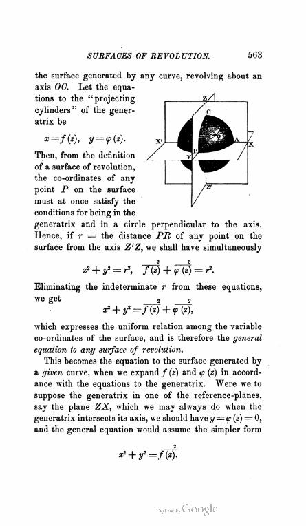
SURFACES OF REVOLUTION. 563
the surface generated by any curve, revolving about an
axis 00. Let the equa
tions to the "projecting zz
cylinders" of the gener
atrix be
*=/(*)> y=f(z)-
Then, from the definition
of a surface of revolution,
the co-ordinates of any
point P on the surface
must at once satisfy the
conditions for being in the
generatrix and in a circle perpendicular to the axis.
Hence, if r — the distance PM of any point on the
surface from the axis Z'Z, we shall have simultaneously
x> + y> = ^, f{z) + <p{z) = r*.
Eliminating the indeterminate r from these equations,
we get 2 2
which expresses the uniform relation among the variable
co-ordinates of the surface, and is therefore the general
equation to any surface of revolution.
This becomes the equation to the surface generated by
a given curve, when we expand / (z) and <p (z) in accord
ance with the equations to the generatrix. Were we to
suppose the generatrix in one of the reference -planes,
say the plane ZX, which we may always do when the
generatrix intersects its axis, we should have y — (p(z) — 0,
and the general equation would assume the simpler form

564 ANALYTIC GEOMETRY.
In this, we suppose the axis of z to be the axis of
revolution ; but, obviously, analogous equations of revo
lution about the axis of x or of y are
2/2 + z2=/», z2 + z2=/(y).
733. Equation to the Right Circular Cone.—Let
the axis of the cone be the axis of z, and its base the
plane XY. Then, if the co-ordinates of the vertex be
x' -— 0, z' = c, the equation to the generatrix (Art. 101,
Cor. 1) will be x~m(z— e), where (Art. 705) m— cot^,
if cp — the inclination of the side to the base of the cone.
Hence
/(2) = ta^5
and, substituting in the equation of revolution, we get
(x2 -f- y2) tan2 f = (z — cf
as the required equation to a right circular cone.
734. Section of a Right Circular Cone by any
Plane.—Since the sections formed by parallel planes
are similar (Art. 714), it will be
sufficient to consider the section
formed by any plane NBL passing
through the axis of y. As this
plane is projected upon the plane
ZX in the line OL, its equation
may be written v
z — x tan d,
where x = OQ, the abscissa of
any point P in the plane ; z = Q31, the corresponding
ordinate ; and 6 = the angle A'OL, which measures the
THE CONE AND ITS SECTIONS. 565
inclination of the plane to the plane XY. Substituting
for z in the above equation to the cone, we obtain
(3? + y2) tan 2 <p = (x tan 6 — c)2,
the equation to the curve of section NBL. Transform
ing this to its own plane, we shall have, in the formulas
of Art. 685, a = 0, ft = 90° ; a' = 90°, /?' = 0 ; a" = 90°,
ft"z=9Q°. We therefore replace x by x cos 6, and leave
y unchanged, thus obtaining, as the equation to any
plane section of a right circular cone,
x2 (tan2 <p — tan2 0) cos2 d + y2 tan2 <p + 2cx sin 0 = c2,
in which tp = the angle OAC, and 0 — the angle A!Oh.
735. The Curves of the Second Order are Con
ies.—The proof of this theorem, promised in Art. 633,
is furnished by the equation just obtained. For this
evidently conforms to the type
Ax2 + 2Hxy + By2 + 2Gx + 2Fy + C= 0,
giving to the -general co-efficients the particular values
A = (tan2 <p — tan2 0) cos2 0, H=Q, B = tan2 <p,
G = c sin d, F =0, C^ — c2.
It therefore denotes a curve of the Second order, whose
species, depending on the sign of H2 — AB, in fact here
depends on the sign of A ; since B7=0, and B is neces
sarily positive.
I. Let A be positive. The function H2 — AB will
then be negative, and (Art. 158) the section will be an
ellipse. But if A is positive, tan2 0 must be less than
tan2 <p ; or, we shall have
9<f.

566 ANALYTIC GEOMETRY.
That is, If the inclination of the secant plane be less than
that of the side of the cone, the section will be an ellipse.
1. One form of the condition 0 < <p is 0 = 0. But
under this supposition, the equation to the section
assumes the form
*2 + y2 — c2 c°t2 <P->
and we obtain a circle, as a particular case of the Ellipse.
2. If under the condition d < <p, we suppose c = 0,
or that the secant plane passes through the vertex of
the cone, the section becomes
3? (tan2 ip — tan2 6) cos2 0 + y2 tan2 <p — 0,
and we have a point, as the limiting case of the Ellipse.
II. Let yl = 0. The function H2—AB will then also
equal 0, and (Art. 191) the section will be a parabola.
When A = 0, however, tan2 6 = tan2 <p ; or,
0 = <p.
That is, If the secant plane be parallel to the side of the
cone, the section will be a parabola.
1. If we suppose 6 — <p — 90°, and c = oo, the equa
tion to the section can readily be put into the form
y2 — constant ; and we learn that when the vertex of the
cone recedes to infinity, the Parabola breaks up into two
parallels.
2. If 0 = <p, and c = 0, the equation to the section
becomes y2 = 0, showing that the limiting case of the
Parabola is a right line.
III. Let A be negative. The function H2 — AB will
then also be negative, and (Art. 174) the section will be
an hyperbola. But if A is negative, tan2 0 > tan2 <p ; or,
6><p.

THE CYLINDER AND THE SPHERE. 567
That is, If the inclination of the secant plane be greater
than that of the side of the cone, the section will be an
HYPERBOLA.
1. If 0 > tp, and be at the same time of such a value
that (tan2 <p — tan2 d) cos2 6 + tan2 <p = 0, the equation to
the section will satisfy the condition A + B = 0, and
the section (Art. 177) will be a rectangular hyperbola.
2. If 0 > <p, and c = 0, so that the secant plane passes
through the vertex, the section becomes
x2 (tan2 f — tan2 8) cos2 6 — y2 tan2 <p = 0,
and the limiting case of the Hyperbola appears as a
pair of intersecting right lines.
We have thus shown that every real variety of the
curve of the Second order can be cut from a right cir
cular cone by a plane. The imaginary varieties, of
course, can not be obtained by any geometric process.
736. Equation to the Circular Cylinder.—The
generatrix of this surface is a right line parallel to the
axis: hence, if we take the latter for the axis of z, the
generatrix will be represented by x — a. We have, then,
/(z) = constant = a ; and the required equation (Art. 732)
is x2 + f = a2,
in which a is the radius of the base.
737. Equation to the Sphere.—Taking the plane
of the generating circle for the plane ZX, the equation
to the generatrix is x2 + z2 = t2. Hence,
/(ijW-z*,
which substituted in the equation of Art. 732 gives
x* + V2 + 22 == f*2-
as the equation now required.
An. Ge. 51.

568 ANALYTIC GEOMETRY.
738. Equations to the Ellipsoids of Revolu
tion.—Let the plane of the generating ellipse be the
plane XY. The equation to the generatrix will be
b'-x2 + a2y2 — a2b2 : whence
7® =
Supposing then the axis major to be the axis of revo
lution, and therefore substituting in the equation for
revolution about the axis of x, we get
- -l y2 + 22 — i
the equation to the Prolate Spheroid.
If the generatrix lie in the plane ZX, its equation
may be written crx2 + a2z2 = a2c2, and we have
/(z) = J(c2-s2)-
Then, taking the axis minor for the axis of revolution,
we substitute in the equation for revolution about the
axis of z, and obtain
■ x2-\-y2 ,z2__,
~~oT~ + ? _ '
the equation to the Oblate Spheroid.
739. Equations to the Hyperboloids of Revolu
tion.—Changing the signs of b2 and c2 in the expressions
of the preceding article for / (xf and / (z)2, we find
THE HYPERBOLOID AND THE PARABOLOID. 569
Supposing the hyperbola to revolve about its trans
verse axis, we substitute in the equation for revolution
about the axis of x, and obtain
x2 _ y2 + z2 _ 1
a2 b2 ~ '
the equation to the Hyperboloid of Revolution of Two
Nappes.
Substituting in the equation for revolution about the
axis of z, which here implies that the hyperbola revolves
about its conjugate axis, we get
z2+ y2 z2 _ 1
~~a~2 ? ~ '
the equation to the Hyperboloid of Revolution of One
Nappe.
740. The Ellipse of the Gorge.—This name is
given to the curve cut from the narrowest part of the
throat of an hyperboloid of one nappe by a plane per
pendicular to its axis. Its equation, found by putting
z= 0 in the equation to the hyperboloid (Art. 728, II), is
£ + £ - 1a2 r b2
In the Hyperboloid of Revolution, this curve becomes
the circle x2 + y2 = a2, which is called the Circle of the
Gorge.
741. Equation to the Paraboloid of Revolu
tion.—Beginning with the generatrix in the plane XY,
its equation is y2 = 4px : whence
2
f(x)=4px,
570 ANALYTIC GEOMETRY.
which, substituted in the equation for revolution about
the axis of x, gives
y2 + z2 = 4px,
the required equation to the generated surface.
TANGENT AND NORMAL PLANES TO THE QUADEICS.
742. General equation to the Tangent Plane.—By
reverting to the vectorial equation near the beginning of
Art. 718, it will be seen that the radius vector will meet
the Quadric in two consecutive points at the origin, if
when 0= 0 we also have
G cos a + jPcos /3 + D cos y = 0.
That is to say, multiplying through by p, and then sub
stituting the corresponding x, y, z, every right line in the
plane
Gx + Fy + Dz = 0
is a tangent to the surface at the origin. Hence, the
equation just written is the equation to the tangent plane
at the origin.
Supposing the origin not to be on the surface, by
transforming to any point x'y'z' of the surface, the
equation to the tangent plane at such point would be,
after putting for the new G, F, D their values as given
in Art. 716,
xUJ + yUJ + zU/ = 0,
which, by re-transformation to the original axes, gives
(x - x>) UJ + (y-y') U> +(z- z') UJ = 0,

TANGENT AND NORMAL PLANES. 571
as the general equation to the tangent plane at any point
x'yV.
Remark.—The generic interpretation of this equation,
as of its analogue in the Conies, is to regard it as the
symbol of the polar plane of the point x'y'z', which in
this view is not restricted to being a point upon the
surface.
743. Tangent Planes to the different Quad-
rtak—The equations to these, in their simplest forms,
are found by deriving UJ, UJ, UJ in the equations
of Arts. 728, 729, and substituting the results in the
general equation last obtained. In this way, we get
x'x y'y ,z'z_.
which represents, in terms of the semi-axes, the tangent
plane to any ellipsoid;
^1 _i_ tl _ — — 1
a2 + b2 c2 '
which represents the tangent plane to any hyperboloid of
one nappe;
x'x y'y z'z 1
~aF ~ ~W ~~ !? ~ '
which represents the tangent plane to any hyperboloid of
two nappes;
2(y'y+Qz'z) = P(x+x>),
which represents the tangent plane to any paraboloid.
744. Normal of a Quadric.—The right line per
pendicular to any tangent plane at its point of contact

572 ANALYTIC GEOMETRY.
with a quadric, is called the normal of the surface at
that point. Hence, by comparing Arts. 709, 742, we
learn that
x — x1 y — y' z — z'
TJi = TP ~ V
are the general equations to the normal at any point x' y' z'.
By deriving UJ, UJ, UJ in the equations of Art. 728,
we obtain the equations to the normals of the central
quadrics, namely,
a2 (x — x') b2 (y — y') c2 (z — z')
x y' z'
in which we must use the upper or lower signs in ac
cordance with the variety of the surface. If we derive
UJ, UJ, UJ in the equation of Art. 729, we obtain
x — x' y' —■ y z' — z
JJ = ~2y~ = 2Qz' '
as the equations to the normal of a paraboloid. These
can of course be thrown into other forms when con
venient.
745. Normal Planes.— Any plane that passes
through the normal of a quadric at any point, is called
a normal plane to the quadric. Comparing Arts. 698
and 744, we learn that the general equation to a normal
plane will be of the form
I (x — x1) m (y — y') (Z + m) (z — z')
IP ' IT1 = IT' '
where the arbitrary k of Art. 698 is for the sake of
symmetry replaced by the ratio m : I.
By deriving UJ, UJ, UJ from any specific equation
to either of the quadrics, and substituting the results in
\\

EXAMPLES. 573
the preceding formula, we can obtain the equation to a
normal plane for any given quadric in any given system
of reference.
It is noticeable that the above equation involves the
indeterminate ratio m : I. This is as it should be ; for
there is obviously an infinite number of normal planes
corresponding to any point on a quadric. When the
normal plane, however, satisfies such conditions as de
termine it, we can readily find the corresponding value
of m : I.
EXAMPLES ON THE QUADKICS.
1. Determine, by means of their discriminating cubies (see Art.
726), whether the quadrics
7a:2 + 6y + 5z2 — \yz — ixy = 6,
7a;2 — 1 3y2 + 6z2 + 24zy + Vlyz — \2zx = ± 84,
2x* + 3ya + 4s2 + 6xy + 4yz + Szx = 8,
are ellipsoids, hyperboloids, or paraboloids.
2. In any central quadric, the sum of the squares on three conju
gate semi-diameters is constant.
3. The parallelopiped whose edges are three conjugate semi-
diameters, is of constant volume.
4. Tangent planes at the extremities of a diameter, are parallel.
5. The length of the central perpendicular upon a tangent plane
is given by the equation
p> ~ a* + b* + <* '
6. The length of the same perpendicular, in terms of its direction-
cosines, is
p2 = a2 cos2 a -|- 42 cos2 /3 + c2 cos2 y.
7. The sum of the squares on the perpendiculars to any three
tangent planes is constant

574 ANALYTIC GEOMETRY.
8. The locus of the intersection of three tangent planes which
are mutually perpendicular, is the sphere
:c2 + .V2 + ;s2 = a2+42 + <:2
9. Find the equation to a diametral plane conjugate to a fixed
point x'y'z'; and prove that if two diameters are conjugate, their
direction-cosines fulfill the condition
cos a cos a' cos ft cos /J' cosy cosy .a< + A5 + T~ = °'
10. The locus of the intersection of three tangent planes at the
extremities of three conjugate diameters is the central quadric

rs \
I


Copyright © 2022 FDOKUMEN