An elementary treatise on the differential calculus : containing the ...
496
-
Upload
khangminh22 -
Category
Documents
-
view
3 -
download
0
Transcript of An elementary treatise on the differential calculus : containing the ...


€ titntnj af
dVUenr
JlrrstuM bxi \l(»»,ii„^«M,,T ^, CV^ cr^aMm\
ill
x?%&5&& >UWGl.^Wkt


AN ELEMENTARY TREATISE
ON
THE DIFFERENTIAL CALCULUS.

AN ELEMENTARY TREATISEON
THE INTEGRAL CALCULUS,CONTAINING
APPLICATIONS TO PLANE CURVES AND SURFACES,AND
A CHAPTER ON THE CALCULUS OF VARIATIONS.
BY
BENJAMIN WILLIAMSON, D.C.L., F.R.S.
Crown 8vo, 10s. 6d.
AN INTRODUCTION TO THE THEORYOF
STRESS AND STRAIN OF ELASTIC SOLIDSBY
BENJAMIN WILLIAMSON, D.C.L., F.R.S.
Crown 8yo, 5s.
AN ELEMENTARY TREATISE ON DYNAMICS,CONTAINING
APPLICATIONS TO THERMODYNAMICS.BY
BENJAMIN WILLIAMSON, D.C.L., F.R.S.,
AND
FRANCIS A. TARLETON, LL.D.
Crown 8vo, 10s. 6d.
LONGMANS, GREEN, AND CO.,
LONDON, NEW YORK, BOMBAY, AND CALCUTTA,

AN ELEMENTARY TREATISE
ON
THE DIFFERENTIAL CALCULUS,
CONTAINING
THE THEORY OF PLANE CURVES,
WITH
NUMEROUS EXAMPLES.
BY
BENJAMIN WILLIAMSON, M.A., D.C.L., Sc.D.,
SENIOR FELLOW OF TRINITY COLLEGE, DUBLIN.
NEW IMPRESSION.
LONGMANS, GREEN, AND CO.,
39 PATERNOSTER ROW, LONDON;
NEW YORK, BOMBAY, AND CALCUTTA.
1912.
[all rights reserved.]
^s^eU)
^TH
PREFACE.
In the following Treatise I have adopted the method of
Limiting Ratios as my basis ; at the same time the co-
ordinate method of Infinitesimals or Differentials has been
largely employed. In this latter respect I have followed in
the steps of all the great writers on the Calculus, from
Newton and Leibnitz, its inventors, down to Bertrand, the
author of the latest great treatise on the subject. An ex-
clusive adherence to the method of Differential Coefficients
is by no means necessary for clearness and simplicity ; and,
indeed, I have found by experience that many fundamental
investigations in Mechanics and Geometry are made more
intelligible to beginners by the method of Differentials than
by that of Differential Coefficients. While in the more ad-
vanced applications of the Calculus, which we find in such
works as the Mecanique Celeste of Laplace and the Mica-
nique Analytique of Lagrange, the investigations are all
conducted on the method of Infinitesimals. The principles
on which this method is founded are given in a concise form
in Arts. 38 and 39.
In the portion of the book devoted to the discussion of
Curves I have not confined myself exclusively to the ap-
plication of the Differential Calculus to the subject, but
have availed mvself of the methods of Pure and Analytic

vi Preface.
Geometry whenever it appeared that simplicity would be
gained thereby.
In the discussion of Multiple Points I have adopted the
simple and general method given by Dr. Salmon in his
Higher Plane Carves. It is hoped that by this means the
present treatise will be found to be a useful introduction to
the more complete investigations contained in that work.
As this book is principally intended for the use of begin-
ners I have purposely omitted all metaphysical discussions,
from a conviction that they are more calculated to perplex
the beginner than to assist him in forming clear conceptions.
The student of the Differential Calculus (or of any other
branch of Mathematics) cannot expect to master at once all
the difficulties which meet him at the outset ; indeed it is only
after considerable acquaintance with the Science of Geometry
that correct notions of angles, areas, and ratios are formed.
Such notions in any science can be acquired only after
practice in the application of its principles, and after patient
study. •
The more advanced student may read with profit Carnot's
Reflexions sur la Mitaphysique da Calcal Infinitesimal; in
which, after giving a complete resume of the different points
of view under which the principles of the Calculus may be
regarded, he concludes as follows :
—
" Le m^rite essentiel, le sublime, on peut le dire, de la
methode infinitesimale, est de reunir la facilite des procedes
ordinaires d'un simple calcul d'approximation a l'exactitude
des resultats de l'analyse ordinaire. Cet avantage immense
serait perdu, ou du moins fort diminue, si a cette methode
pure et simple, telle que nous l'adonnee Leibnitz, on voulait,
sous l'apparence d'une plus grande rigueur soutenue dans
tout le cours de calcul, en substituer d'autres moins naturelles,
Preface. vii
moins commodes, moins conform es a la marehe probable
des inventeurs. Si cette methode est exacte dans les re-
sultats, comme personne n'en doute aujourd'hui, si c'est tou-
jours a elle qu'il faut en revenir dans les questions difficiles,
comme il parait encore que tout le monde en convient,
pourquoi recourir a des moyens detournes et compliques pour
la suppleer? Pourquoi so contenter de l'appuyer sur des
inductions et sur la conformite de ses resultats avex ceux que
fournissent les autres methodes, lorsqu'on peut la demontrer
directement et generalement, plus facilement peut-etre
qu'aucune de ces methodes elles-memes ? Les objections que
Ton a faites contre elle portent toutes sur cette fausse suppo-
sition que les erreurs commises dans le cours du calcul, en ynegligeant les quantites infiniment petites, sont demeurees
dans le resultat de ce calcul, quelque petites qu'on les sup-
pose ; or c'est ce qui n'est point : Telimination les emporte
toutes necessairement, et il est singulier qu'on n'ait pas
apercu d'abord dans cette condition indispensable de Telimi-
nation le veritable caractere des quantites infinitesimales et
la reponse dirimante a toutes les objections."
Many important portions of the Calculus have been
omitted, as being of -too advanced a character ; however,
within the limits proposed, I have endeavoured to make the
Work as complete as the nature of an elementary treatise
would allow.
I have illustrated each principle throughout by copious
examples, chiefly selected from the Papers set at the various
Examinations in Trinity College.
In the Chapter on Eoulettes, in addition to the discussion
of Cycloids and Epicycloids, I have given a tolerably com-
plete treatment of the question of the Curvature of a Eoulette,
as also that of the Envelope of any Curve carried by a rolling

viii Preface.
Curve. This discussion is based on the beautiful and general
results known as Savary's Theorems, taken in conjunction
with the properties of the Circle of Inflexions. I have
introduced the application of these theorems to the general
case of the motion of any plane area supposed to move on
a fixed Plane.
I have also given short Chapters on Spherical Harmonic
Analysis and on the System of Determinant Functions
known as Jacobians, which now hold so fundamental a place
in analysis.
Trinity College,
October, 1899.

TABLE OF CONTENTS.
CHAPTER I.
FIRST PRINCIPLES. DIFFERENTIATION.
FAGHDependent and Independent Variables, I
Increments, Differentials, Limiting Ratios, Derived Functions, . . 3Differential Coefficients, 5Geometrical Illustration, ......... £
Navier, on the Fundamental Principles of the Differential Calculus, . 8
On Limits, ............ 10
Differentiation of a Product, ^ 13
Differentiation of a Quotient, . . . . • . . . • 15
Differentiation of a Power, . . . . . . . . .16Differentiation of a Function of a Function, . . . . . 1
7
Differentiation of Circular Functions, 19
Geometrical Illustration of Differentiation of Circular Functions, . . 22
Differentiation of a Logarithm, 24Differentiation of an Exponential, ........ 26
Logarithmic Differentiation, 27Examples, 30
CHAPTEK II,
SUCCESSIVE DIFFERENTIATION,
Successive Differential Coefficients,
Infinitesimals,
Geometrical Illustrations of Infinitesimals,
Fundamental Principle of the Infinitesimal Calculus,
Subsidiary Principle, .....Approximations, ......Derived Functions of xm
,....
Differential Coefficients of an Exponential,
Differential Coefficients of tan-1x> and tan" 1 -, .
xTheorem of Leibnitz,
Applications of Leibnitz's Theorem,Examples, ... .
3436
37404i
424648
50
5'
53
57
Table of Contents.
CHAPTER III.
DEVELOPMENT OF FUNCTIONS.
Taylor's Expansion, .
Binomial Theorem, ,
Logarithmic Series, .
Maclaurin's Theorem, ....Exponential Series, ....Expansions of sin x and cos x,
Huy gens' Approximation to Length of Circular
Expansions of tan" 1 x and sin"1#,
Euler's Expressions for sin x and cos xf .
John Bernoulli's Series,
Symbolic Form of Taylor's Series, .
Convergent and Divergent Series, .
Lagrange's Theorem on the Limits of Taylor's
Geometrical Illustration,
Second Form of the Remainder,General Form of Maclaurin's Series,
Binomial Theorem for Fractional and NegativeExpansions by aid of Differential Equations,
Expansion of sin mz and cos mzy
Arbogast's Method of Derivation,
Examples, ......
Arc,
Series,
Indices,
PAGH61
63636465666668
697o
70
n76
78
7981
82
8587S8
9*
CHAPTEK IV.
INDETERMINATE FORMS.
Examples of Evaluating Indeterminate Forms without the Differential
,
Calculus,............ 96Method of Differential Calculus, ........ 99Form Oxoo, , . . . . 102
Form 22., ..,..103Forms o°, 00 °, i
±flD., , * . .105
Examples, 109
CHAPTER V.
PARTIAL DIFFERENTIAL COEFFICIENTS.
Partial Differentiation, . .
Total Differentiation of a Function of Two Variables,
Total Differentiation of a Function of Three or more Variables,
Differentiation of a Function of Differences,
Implicit Functions, Differentiation of an Implicit Function,
Euler's Theorem of Homogeneous Functions, .
Examples in Plane Trigonometry, .....Landen's Transformation,
Examples in Spherical Trigonometry, ....Legendre's Theorem on the Comparison of Elliptic Functions,
Examples, .........
"3"5"7119120
123
130
13714c

Table of Contents. XI
CHAPTER VI.
SUCCESSIVE PARTIAL DIFFERENTIATION.
The Order of Differentiation is indifferent in Independent Variables,
Condition that Pdx -f Qdy should be an exact Differentia],
Euler's Theorem of Homogeneous Functions,Successive Differential Coefficients of <p (x -+- at, y -f fit),
Examples, .........
PAGE
145I46
I48
I48
'50
CHAPTER VII.
lagrange's theorem.
Lagrange's Theorem, 151Laplace's Theorem, ., . 154Examples, 155
CHAPTER VIII.
extension of taylor's theorem.
Expansion of <p {x + //, y + /•), . 156Expansion of
<f>(x + h
t y -\ k, z + /), . . . . . , 159Symbolic Forms, .160Euler's Theorem, 162
CHAPTER IX.
maxima and minima for a single variable,
Geometrical Examples of Maxima and Minima,Algebraic Examples, .....Criterion for a Maximum or a Minimum,Maxima and Minima occur alternately, .
Maxima or Minima of a Quadratic Fraction, .
Maximum or Minimum Section of a Right Cone,Maxima or Minima of an Implicit Function, .
Maximum or Minimum of a Function of Two Dependent Variables,
Examples,
164
165
169
173
*77181
185186
188
CHAPTER X.
maxima and minima of functions of two or more variables.
Maxima and Minima for Two Variables,
Lagrange's Condition in the case of Two Independent Variables,
191
191

xii Table of Contents.
PageMaximum or Minimum of a Quadratic Fraction, 194Application to Surfaces of Second Degree, . . . . .196Maxima and Minima for Three Variables, 198Lagrange's Conditions in the case of Three Variables, . . . . 199Maximum or Minimum of a Quadratic Function of Three Variables, . 200Examples, ............ 203
CHAPTER XL
METHOD OF UNDETERMINED MULTIPLIERS APPLIED TO MAXIMA ANDMINIMA.
Method of Undetermined Multipliers, 204Application to find the principal Radii of Curvature on a Surface, . . 208Examples, 210
CHAPTER XII.
ON TANGENTS AND NORMALS TO CURVES.
Equation of Tangent, . . . . . . . . . .212Equation of Normal, 215Subtan gent and Subnormal, . . . . . . . . . 215Number of Tangents from an External Point, 219Number of Normals passing through a given Point, .... 220Differential cf an Arc, 220Angle between Tangent and Radius Vector, ...... 222
Polar Subtangent and Subnormal, ....... 223Inverse Curves, . . . . . . . . . . .225Pedal Curves, 227Reciprocal Polars, 228
Pedal and Reciprocal Polai of rm = am cos m$, ..... 230Intercept between point of Contact and foot of Perpendicular, . . 232Direction of Tangent and Normal in Vectorial Coordinates, . . . 233Symmetrical Curves, and Central Curves, 236Examptea. 238
CHAPTER XIII.
ASYMPTOTES.
Points of Intersection of a Curve and a Right Line, .... 240Method of Finding Asymptotes in Cartesian Coordinates, . . .242Case where Asymptotes all pass through the Origin, .... 245Asymptotes Parallel to Coordinate Axes, 245Parabolic and Hyperbolic Branches, . . . . . . 246Parallel Asymptotes, . . . . . . . . . -247The Points in which a Cubic is cut by its Asymptotes lie in a Right Line, 249Asymptotes in Polar Curves, 250Asymptotic Circles, 252Examples, ......•••••• 254

Table of Contents. xiii
CHAPTEK XIV.
MULTIPLE POINTS ON CURVES.
TageNodes, Cusps, Conjugate Points, 259Method of Finding Double Points in general, 26 1
Parabolas of the Third Degree, 262Double Points on a Cubic having three given lines for its Asymptotes, . 264Multiple Points of higher Orders, 265Cusps, in general, .......... 266Multiple Points on Curves in Polar Coordinates, 267Examples, •••• 268
CHAPTEK XV.
ENVELOPES.
Method of Envelopes, 270Envelope of La2
-f 2Ma +N = O, 271Undetermined Multipliers applied to Envelopes, 273Examples, # 276
CHAPTEE XVI.
CONVEXITY, CONCAVITY, POINTS OF INFLEXION.
Convexity and Concavity, . .278Points of Inflexion, .......... 279Harmonic Polar of a Point of Inflexion on a Cubic, . . . .281Stationary Tangents, 282Examples, 283
CHAPTEK XVII.
RADIUS OF CURVATURE, EVOLUTES, CONTACT,
Curvature, Angle of Contingence, 285Radius of Curvature, . 286Expressions for Eadius of Curvature, 287Newton's Method of considering Curvature, • . . . . .291Radii of Curvature of Inverse Curves, 295Radius and Chord of Curvature in terms of r and p y
.... 295Chord of Curvature through Origin, 296Evolutes and Involutes, 297Evolute of Parabola, 298Evolute of Ellipse, 299Evolute of Equiangular Spiral, 300

XIV Table of Contents.
Involute of a Circle, ,™Radius of Curvature and Points of Inflexion in Polar Coordinates, . .301Intrinsic Equation of a Curve, ^oiContact of Different Orders, [ <,Q t
Centre of Curvature of an Ellipse,*
? 7Osculating Curves,
9oQg
Radii of Curvature at a Node, . . . . . . . .210Radii of Curvature at a Cusp, . . . . . , , . 311At a Cusp of the Second Species the two Radii of Curvature are equal, . 312General Discussion of Cusps, . . . . . . .
*t c
Points on Evolute corresponding to Cusp3 on Curve, . , . .316Equation of Osculating Conic, . . . . , „ . .317Examples,
r m . ?io
CHAPTEE XVIII.
ON TRACING OF CURVES.
Tracing Algebraic Curves,Cubic with three real Asymptotes,Each Asymptote corresponds to two Infinite Branches,Tracing Curves in Polar Coordinates,On the Curves rm =«"» cos md,The Limacon,The Conchoid,Examples, ....
322
323325328328
3V332
333
CHAPTEE XIX.
ROULETTES.
Roulettes, Cycloid, 33-Tangent to Cycloid,
! ! 336Radius of Curvature, Evolute, 337Length of Cycloid, ]
*333
Trochoids, • * . 339Epicycloids and Hypocycloids, 339Radius of Curvature of Epicycloid, . 342Double Generation of Epicycloids and Hypocycloids, .... 343Evolute of Epicycloid,
344Pedal of Epicycloid,
m 346Epitrochoid and Hypotrochoid, 347Centre of Curvature of Epitrochoid, . . . . . '.
. 351Savary's Theorem on Centre of Curvature of a Roulette, . . . .352Geometrical Construction for Centre of Curvature, 352Circle of Inflexions, .......... 354Envelope of a Carried Curve, 355Centre of Curvature of the Envelope, .... ^57
Table of Contents, xv
Radius of Curvature of Envelope of a Right Line,
On the Motion of a Plane Figure in its Plane,
Chasles' Method of Drawing Normals, .
Motion of a Plane Figure reduced to Roulettes,
Epicyclics, ....Properties of Circle of Inflexions,
Theorem of Bobilier,
Centre of Curvature of Conchoid,
Spherical Roulettes,
Examples, • • • •
PAGE35?
359360362
36336736837o
370372
CHAPTER XX.
ON THE CAKTESIAN OVAL.
Equation of Cartesian Oval, 375Construction for Third Focus, 376Equation, referred to each pair of Foci, . 377Conjugate Ovals are Inverse Curves, 378Construction for Tangent, . . . . • . . . 379Confocal Curves cut Orthogonally, 381Cartesian Oval as an Envelope, 382Examples, 384
CHAPTER XXI.
ELIMINATION OF CONSTANTS AND FUNCTIONS.
Elimination of Constants, 384Elimination of Transcendental Functions, 386Elimination of Arbitrary Functions, 387Condition that one expression should be a Function of another, . . 389Elimination in the case of Arbitrary Functions of the same expression, . 393Examples, 397
CHAPTER XXII.
CHANGE OF INDEPENDENT VAKIABLE,
Case of a Single Independent Variable, 399Transformation from Rectangular to Polar Coordinates, .... 403
d2 V d2 VTransformation of -—- + —— , 404
dx2 dyl
m . .. »&V d2 V d2 VTransformation of ——- + —— + —-, 405
dx2 dy2 dz2
Geometrical Illustration of Partial Differentiation, 407

xvi Table of Contents.
PAGELinear Transformations for Three Variables, ...... 408Case of Orthogonal Transformations, ....... 409General Case of Transformation for Two Independent Variables, . .410Functions unaltered by Linear Transformations, 411Application to Geometry of Two Dimensions, 412Application to Orthogonal Transformations, 414Examples, 416
CHAPTER XXIII.
SOLID HAKMONIC ANALYSIS.
d?V d2 V d2 VOn the Equation—+—+— = 0, 418
Solid Harmonic Functions, 419Complete Solid Harmonics, 421Spherical and Zonal Harmonics, ........ 423Complete Spherical Harmonics, . . . . . . . . 427Laplace's Coefficients, 429Examples, 432
CHAPTER XXIV.
JACOBIANS.
Jacobians, 433Case in which Functions are not Independent, 435Jacobian of Implicit Functions, .... .... 438Case where / = o, . . . 44
1
Case where a Relation connects the Dependent Variables, . . . 442Examples, 446
CHAPTER XXV.
GENERAL CONDITIONS FOR MAXIMA AND MINIMA.
Conditions for Four Independent Variables, 447Conditions for n Variables, 449Orthogonal Transformation, ......... 452
Miscellaneous Examples, 454Note on Failure of Taylor's Theorem, 467
The beginner is recommended to omit the following portions on the Jirst
reading :—Arts. 49, 50, 51, 52, 67-85, 88, III, 114-116, 124, 125, Chap, vn.,Chap. viii. ; Arts. 159-163, 249-254, 261-269, 296-301, Chaps, xxiii.,
XXIV., XXV.
DIFFEEENTIiL CALCULUS,
CHAPTER I.
FIRST PRINCIPLES DIFFERENTIATION
.
i . Functions.—The student, from his previous acquaintance
with Algebra and Trigonometry, is supposed to understand
what is meant when one quantity is said to be a function of
another. Thus, in trigonometry, the sine, cosine, tangent, &c,of an angle are said to be functions of the angle, having each
a single value if the angle is given, and varying when the
angle varies. In like manner any algebraic expression in x
is said to be a function of x. Geometry also furnishes us
with simple illustrations. For instance, the area of a square,
or of any regular polygon of a given number of sides, is afunction of its side ; and the volume of a sphere, of its radius.
In general, whenever two quantities are so related, that
any change made in the one produces a corresponding variation
in the other, then the latter is said to be a function of the
former.
This relation between two quantities is usually represented
by the letters F, /, 0, &c.
Thus the equations
U-F(9), *=/(#), I0«0(J?),
denote that u, v, w, are regarded as functions of x, whosevalues are determined for any particular value of x, when the
form of the function is known.2. Dependent and Independent Variables, Con-
stants.—In each of the preceding expressions, x is said to be6

2 First Principles—Differentiation.
the independent variable, to which any value may be assigned
at pleasure ; and «, v, w, are called dependent variables, as their
values depend on that of xyand are determined when it is
known.Thus, in the equations
V - 10*, y = x>, y = sm(P,
the value of y depends on that of #, and is in each case deter-
mined when the value of x is given.
If we suppose any series of values, positive or negative,
assigned to the independent variable x, then every function
of x will assume a corresponding series of values. If a quan-tity retain the same value, whatever change be given to x, it
is said to be a constant with respect to x. We usually denoteconstants by a, J, c, &c, the first letters of the alphabet
;
variables by the last, viz., u9v, w, x, y, z.
3. Algebraic and Transcendental Functions.—Functions which consist of a finite number of terms, involving
integral and fractional powers of x, together with constants
solely, are called algebraic functions—thus
are algebraio expressions.
Functions which do not admit of being represented as
ordinary algebraic expressions in & finite number of terms are
called transcendental : thus, sin x, cos x, tan a?, 0*, log x, &c,are transcendental functions ; for they cannot be expressed
in terms of x except by a series containing an infinite numberof terms.
Algebraic functions are ultimately reducible to the follow-
ing elementary forms : (1). Sum, or difference (u + v, u - v).
(2). Product, and its inverse, quotient (uv>-J.
Powers, and
their inverse, roots (wm , um).
The elementary transcendental functions are also ulti-
mately reducible to : (1). The sine, and its inverse, (sin u,
sin" 1
^). (2). The exponential, and its inverse, logarithm
(V, log a). •

Limiting Ratios—Derived Functions. 3
4. Continuous Functions.—A function (x) is said to
be a continuous function of x, between the limits a and b,
when, to each value of x, between these limits, corresponds a
finite value of the function, and when an infinitely small
change in the value of x produces only an infinitely small
change in the function. If these conditions be not fulfilled
the function is discontinuous. It is easily seen that all
algebraic expressions, such as
atf? + diX71"1 4 . . . . any
and all circular expressions, sin x, tan x, &c, are, in general,
continuous functions, as also ex
, log x.:&c. In such cases,
accordingly, it follows that if x receive a very small change,
the corresponding change in the function of x is also very
small.
5. Increments* and Differentials.—In the Differen-
tial Calculus we investigate the changes which any function
undergoes when the variable on which it depends is made to
pass through a series of different stages of magnitude.
If the variable x be supposed to receive any change, such
change is called an increment ; this increment of x is usually
represented by the notation Ax.
When the increment, or difference, is supposed infinitely
small it is called a differential, and represented by dx, i.e. an
infinitely small difference is called a differential.
In like manner, if u be a function of x, and x becomesx + Ax, the corresponding value of u is represented by u + Ait
;
i. e. the increment of u is denoted by Au.
6. limiting Ratios, Derived Functions.—If w be a
function of x, then for finite increments, it is obvious that the
ratio of the increment of u to the corresponding increment of
x has, in general, a finite value. Also when the increment
of x is regarded as being infinitely small, we assume that the
ratio above mentioned has still a definite limiting value. Inthe Differential Calculus we investigate the values of these
limiting ratios for different forms of functions.
The ratio of the increment of u to that of x in the limit,
when both are infinitely small, is denoted by — . Whenax
B 2

4 First Principles—Differentiation.
u =/(#), this limiting ratio is denoted by /'(#), and is called
the first derivedfunction* off(x).
Thus ; let x become x + h, where h = A#, then u becomes
f{x + h), i. e. u 4 Aw =f(x + ti),
.\ Aw =f(x + A) -/(*),
Aw f{x + h)-f{x)
A# h
The limiting value of this expression when h is infinitely small
is called the first derived function of /(#), and represented
Again, since the ratio — has/' (a?) for its limiting value,
if we assume
Ai=' {X) + "
a must become evanescent along with Air ; also — becomesAx
— at the same time ; hence we havedx
This result may be stated otherwise, thus :—If u x denotethe value of u when x becomes.^, then the value of the ratio
Ui ~~ u, when xx
- x is evanescent, is called ihe first derivedXi— x
function of u, and denoted by —
.
' J dx
* The method of derived functions was introduced by Lagrange, and thedifferent derived functions off(x) were defined by him to be, the coefficients of
the powers of h in the expansion of/(# + h) : that this definition of the first
derived function agrees with that given in the text will be seen subsequently.
This agreement was also pointed out by Lagrange. See " Theorie des
Fonctions Analytiques," N08. 3, 9.

Algebraic Illustration, 5
If Xi be greater than x, then ux is also greater than u, pro-
vided is positive ; and hence, in the limit, when xx- x
is evanescent, u x is greater or less than u according as — iscix
positive or negative. Hence, if we suppose x to increase,
then any function of x increases or diminishes at the sametime, according as its derived function, taken with respect
to x, is positive or negative. This principle is of great
importance in tracing the different stages of a function of x,
corresponding to a series of values of x.
7. Differential, and Differential Coefficient, of
Let u =/(#) ; then since
we have du = d(f(x)) = f(x)dx,
where dx is regarded as being infinitely small. In this
case dx is, as already stated, the differential of x, and duor f (x) dx, is called the corresponding differential of u.
Also f'{x) is called the differential coefficient of /(#), beingthe coefficient of dx in the differential of f(x).
8. Algebraic Illustration.—That a fraction whosenumerator and denominator are both evanescent, or in-
finitely small, may have a finite determinate value, is
a naevident from algebra. For example, we have T = —7 what-
noever n may be. If n be regarded as an infinitely small
number, the numerator and denominator of the fraction
both become infinitely small magnitudes, while their ratio
remains unaltered and equal to -r.
It will be observed that this agrees with our ordinaryidea of a ratio ; for the value of a ratio depends on the
relative, and not on the absolute magnitude of the termswhich compose it.
Again, ff una + n2
a'
nb + n2b"
in which n is regarded as infinitely small, and a, b9
a' and V

6 First Principles—Differentiation.
represent finite magnitudes, the terms of the fraction are
both infinitely small,
but their ratio is r>,
b + no
the limiting value of which, as n is diminished indefinitely,
is j. Again, if we suppose n indefinitely increased, the
limiting value of the fraction is j-r For
a + an a' ab' - ba
b + Vn b' V (b + Vn)'
It 7 /
but the fraction -rrn—ttt diminishes indefinitely as n
t
V(b + Vn)J
increases indefinitely, and may be made less than anyassignable magnitude, however small. Accordingly the
limiting value of the fraction in this case is Tro
9. Trigonometrical Illustration.—To find the values
of -—g, and —tj— , when is regarded as infinitely email.
Here -—- = cos 0, and when 9 = o, cos 6 = 1
.
tanft
Hence, in the limit, when = o,* we havesin 6 _ tan# . .. ,.: a = 1, and, .\ -;
—
s = 1, at the same time.tan sin
n
Again, to find the value of -—^, when 6 is infinitely small.
From geometrical considerations it is evident that if be
the circular measure of an angle, we have
tan > 6 > sin 0,
tan0or -1—£ > -r—5 > 1
;
sin v sin
* If a variable quantity be supposed to diminish gradually, tiUitbe less than
anything finite which can be assigned, it is said in that state/wbe\ndefinitely
small or evanescent; for abbreviation, such a quantity is often denoted oy,>cypher.
A discussion of infinitesimals, or infinitely small quantities of different orders,
will be found in the next Chapter.

Geometrical Illustration.
but in the limit, i.e. when 9 is infinitely small,
tan0
SnU ~ *'
and therefore, at the same time, we have
6
sin0= i
This shows that in a circle the ultimate ratio of an arc to its
chord is unity, when they are both regarded as evanescent.
10. Geometrical Illustration.—Assuming that the
relation y = f(x) may in all cases be represented by a curve,
wherey = /(*)
expresses the equation connecting the co-ordinates (x, y)of each of its points ; then, if the axes be rectangular, andtwo points (x, y), (%l9 y x) be taken on the curve, it is obvious
that represents the tangent of the angle which theX\ ~~ x
chord joining the points (#, y), (xly y x ) makes with the axis
of x.
If, now, we suppose the points taken infinitely near to
each other, so that xY- x becomes evanescent, then the chord
becomes the tangetit at the point (#, y), but
——- becomes —- or f (x) in this case.xx
- x ax
Hence, f (x) represents the trigonometrical tangent of the
angle tvhich the line touching the curve at the point (x, y) makes
ivith the axis of x. We see, accordingly, that to draw the
tangent at any point to the curve
V - /(*)
is the same as to find the derived function f(x) of y with
respect to x. Hence, also, the equation of the tangent to
the curve at a point (x, y) is evidently
y-Y = f{x){x-X), (2)
where X, Y are the current co-ordinates of any point on the

8 First Principles—Differentiation,
tangent. At the points for which the tangent is parallel to
the axis of x, we have f (x) = o ; at the points where the
tangent is perpendicular to the axis, f (x) = oo . For all
other points f (x) has a determinate finite real value in
general. This conclusion verifies the statement, that the
ratio of the increment of the dependent variable to that of
the independent variable has, in general, a finite determinate
magnitude, when the increment becomes infinitely small.
This has been so admirably expressed, and its con-
nexion with the fundamental principles of the Differential
Calculus so well explained, by M. Navier, that I cannot for-
bear introducing the following extract from his "Leconsd'Analyse":
—
" Among the properties which the function y = f(x), or
the line which represents it, possesses, the most remarkable
—
in fact that which is the principal object of the Differential
Calculus, and which is constantly introduced in all practical
applications of the Calculus—is the
degree of rapidity with which the
function /(#) varies when the in-
dependent variable x is made to
vary from any assigned value.
This degree of rapidity of the
increment of the function, when xis altered, may differ, not only
from one function to another, butalso in the same function, ac-
cording to the value attributed to
the variable. In order to form a
precise notion on this point, let us attribute to x a deter-
mined value represented by ON, to which will correspond
an equally determined value of y, represented by PN. Letus now suppose, starting from this value, that x increases byany quantity denoted by Ax, and represented by NM, the
function y will vary in consequence by a certain quantity,
denoted by Ay, and we shall have
y + Ay = f(x + Ax), or Ay = f(x + Ax) -/(#).
The new value of y is represented in the figure by Q3f,
and QL represents Ay, or the variation of the function.
Fig.

Geometrical Illustration. g
The ratio — of the increment of the function to that ofAx
the independent variable, of which the expression is
/Qg+ Ax) -/(a?)
Ax '
is represented by the trigonometrical tangent of the angle
QPL made by the secant PQ with the axis of x.
Ay44 It is plain that this ratio — is the natural expression
of the property referred to, that is, of the degree of rapidity
with which the function y increases when we increase the
independent variable x ; for the greater the value of this
ratio, the greater will be the increment Ay when x is in-
creased by a given quantity Ax. But it is very important
Avto remark, that the value of —- (except in the case when
Axthe line PQ becomes a right line) depends not only on the
value attributed to x, that is to say, on the position of P onthe curve, but also on the absolute value of the increment Ax.
If we were to leave this increment arbitrary, it would be
impossible to assign to the ratio — any precise value, andL±X
it is accordingly necessary to adopt a convention which shall
remove all uncertainty in this respect.14 Suppose that after having given to Ax any value, to
which will correspond a certain value Ay and a certain
direction of the secant PQ, we diminish progressively the
value of Ax> so that the increment ends by becomingevanescent ; the corresponding increment Ay will vary in
consequence, and will equally tend to become evanescent.
The point Q will tend to coincide with the point P, and the
secant PQ with the tangent PT drawn to the curve at the
Aypoint P. The ratio — of the increments will equally
approach to a certain limit, represented by the trigonometrical
tangent of the angle TPL made by the tangent with the
axis of x.
"We accordingly observe that when the increment Ax}

io First Principles—Differentiation,
and consequently Ay, diminish progressively and tend to
A?/vanish, the ratio — of these increments approaches in
general to a limit whose value is finite and determinate.
A?/Hence the value of — corresponding to this limit must be
i\X
considered as giving the true and precise measure of the
rapidity with which the functionf (x) varies when the independent
variable x is made to vary from an assigned value ; for there
does not remain anything arbitrary in the expression of this
value, as it no longer depends on the absolute values of the
increments Ax and Ay, nor on the figure of the curve at anyfinite distance at either side of the point P. It depends
solely on the direction of the curve at this point, that is, on
the inclination of the tangent to the axis of x. The ratio
just determined expresses what Newton called the fluxion of
the ordinate. As to the mode of finding its value in each
particular case, it is sufficient to consider the general
expressionAy /{x + Ax) . /{x)
Ax Ax
and to see what is the limit to which this expression tends,
as Ax takes smaller and smaller values and tends to vanish.
This limit will be a certain function of the independent
variable #, whose form depends on that of the given function
f(x) "We shall add one other remark ; which is, that
the differentials represented by dx and dy denote always
quantities of the same nature as those denoted by the variables
x and y. Thus in geometry, when x represents a line, an
area, or a volume, the differential dx also represents a line, an
area, or a volume. These differentials are always supposed
to be less than any assigned magnitude, however small ; but
this hypothesis does not alter the nature of these quantities :
dx and dy are always homogeneous with x and y, that is to
say, present always the same number of dimensions of the unit
by means of which the values of these variables are expressed."
10a. Iiimit of a Variable Magnitude.—As the con-
ception of a limit is fundamental in the Calculus, it maybe well to add a few remarks in further elucidation of its
meaning :
—

Limit of a Variable Magnitude. 1
1
In general, when a variable magnitude tends continually to
equality ivith a certain fixed magnitude, and approaches nearer to
it than any assignable difference, hoicever small, this fixed magni-tude is called the limit of the variable magnitude. For example,if we inscribe, or circumscribe, a polygon to any closed curve,
and afterwards conceive each side indefinitely diminished,
and consequently their number indefinitely increased, thenthe closed curve is said to be the limit of either polygon.
By this means the total length of the curve is the limit of
the perimeter either of the inscribed or circumscribed polygon.
In like manner, the area of the curve is the limit to the
area of either polygon. For instance, since the area of anypolygon circumscribed to a circle is obviously equal to the
rectangle under the radius of the circle and the semi-perimeter
of the polygon, it follows that the area of a circle is repre-
sented by the product of its radius and its semi-circumfe-
rence. Again, since the length of the side of a regular
polygon inscribed in a circle bears to that of the correspond-
ing arc the same ratio as the perimeter of the polygon to the
circumference of the circle, it follows that the ultimate ratio
of the chord to the arc is one of equality, as shown in Art. 9.
The like result follows immediately for any curve.
The following principles concerning limits are of fre-
quent application:— (1) The limit of the product of two quan-
tities, which vary together, is the product of their limits; (2) Thelimit of the quotient of the quantities is the quotient of their
limits.
For, let P and Q represent the two quantities, and p and
q their respective limits ; then if
P=p+a, Q = y + i3,
a and j3 denote quantities which diminish indefinitely as Pand Q approach their limits, and which become evanescentin the limit.
Again, we have
PQ = pq + pfi + qa + a(3.
Accordingly, in the limit, we have
PQ =pq.

12 First Principles—Differentiation.
AffainP _p + a _p qa - p(5Agam
' Q-f^ q+far®-
The numerator of the last fraction becomes evanescent in
the limit, while the denominator becomes q2, and consequently
the limit of ~ is -.
Q q1 1 . Differentiation.—The process of finding the derived
function, or the differential coefficient of any expression, is
called differentiating the expression.
We proceed to explain this process by applying it to a
few elementary examples.
Examples.
i. y = x2 .
Substitute x -f h for x, and denote the new value of y by yi, then
yi = (x + h)2 = x2 + 2#A + h2;
*/i - y Ay ..*. ; Or —- = 24? + A.
A Ax
If A be taken an infinitely small quantity, we get in the limit
dy
or if /(») = x2ywe have/' (#) = 2X.
i
i. y = -.a?
Here yia: + A
Vl ~ y "a; + h x~ x (x + A)
'
A As # (a; + A)'
which equation, when ^ iB evanescent, becomes
^ L **' = _ 1.dx~ x* dx x2
°

Differentiation of a Product, 13
12. Differentiation of the Algebraic Sum of aFinite Number of Functions.—Let
y = u -t- v - w + &c.
;
then, if xx= x + A, we get
^i - tti + f>| - 14 + . . .
;
t/\ - V __ Ui - U Vi-V Wi - Wh
=:
~h~+
~~A A~ +' "
"»
which becomes in the limit, when h is infinitely small,
dy du dv dw
dx dx dx dx
Hence, if a function consist of several terms, its derived
function is the sum of the derived functions of its several parts,taken with their proper signs.
It is evident that the differential of a constant is zero.
13. Differentiation of the Product of Two Func-tions.—Let y = uv, where u, v, are both functions of x ; andsuppose Ay, Au, Av, to be the increments of y, u
}v, corre-
sponding to the increment Ax in x. Then
Ay = (u + Au) (v + Av) - uv
= uAv + vAu + Aw Av,
Ay Av Auor — = u — + (v + Av) —
.
A^ Aa!v
' Ax
Now suppose Ax to be infinitely small, then
Ay Av AuAx9 Ax9 Ax9
become in the limit
dy dv du#
dx9
dx9
dx
'
also, since Av vanishes at the same time, the last term dis-
appears from the equation, and thus we arrive at the result
dy dv du
dx"Udx
+ Vdx' ^'

14 First Principles—Differentiation,
Hence, to differentiate the product of two functions,
multiply each of the factors by the differential coefficient of the
other, and add the products thus found.
Otherwise thus: let/(#), (j> (#), denote the functions, andh the increment of #, then
Vi = /(* + h) <t>(x + h);
. yx -y _ f(x + h) <p (x + h) -/(a?) (a?)
" h h
_ f(x + h)-f(x)<p(x + h)-
tf>(x)
Y~— \
x + h) +/ \
x) ^ •
Now, in the limit,
f(x\h) -f{x) .,. -
and <p (a? + A) - $>(#)
A~~ =
* W*
and, accordingly,
|=/(*)f(*W(*)/(*),
which agrees with the preceding result.
When y = au, where a is a constant with respect to #,
we have evidently
cly du
dx dx'
14. Differentiation of the Product of any \umberof Functions.—First let
y = uvw;
suppose
then
vw
y = HZ,
and, by Art. 13, we have
dA =dx
dz
it
duzTx
;

Differentiation of a Quotient. 15
but, by the same Article,
dz dv die
hence
dx dx dx9
dy du dv die
-f- = vw— + wu— + uv—
.
dx dx ax dx
This process of reasoning can be easily extended to anynumber of functions.
The preceding result admits of being written in the form
1 dy 1 du 1 dv 1 dw
y dx u dx v dx tv dx
and in general, if y = y x . y% . y3 . . . . yny
it can be easily proved in like manner that
\_djj_= idfr
+ 1^2 + _i <*Vn t.\
y dx y x dx y2 dx'
yn dx
'
15. Differentiation of a Quotient—Let
y = -, then u = yv\
., p , A . du dv dytherefore, by Art. 13, _ = y_ + „-,
ordy du dv du
dx dx *" dx dx
udv
v dx
du dvv u—dx dx
m ;
V'
du dv
dy dx d»
dx v2
(5)
This may be written in the following form, which is often
useful:
d fu\ 1 du u dv
dx \v ) v dx v2 dx'

16 First Principles—Differentiation.
Hence, to differentiate a fraction, multijily the denominator
into the derivedfunction of the numerator, and the numerator into
the derived function of the denominator ; take the latter product
from the former, and divide by the square of the denominator.
In the particular case where u is a constant with respect
to x {a suppose), we obviously have
i.
2.
d fa\ a dv(6)
dx \v) ft1dx'
Examples.a-x A *U 2<l
u = .
a+ s dx (a + xf
u = (a + x) (* + *).du— = a -f o + 2X.dx
1 6. Differentiation of an Integral Power.—Let
y = #», where n is a positive integer.
Suppose y x to be the value of y, when x becomes xu then
Xx- X Xi - X
Now, suppose Xi - x to be evanescent. In this case wemay write x for xx in the right-hand side of the preceding
equation, when it becomes nxn~x
\ but the left-hand side, in
the limit, is represented by — •
Hence -£- = Hof1,
or -^r1 = nx"~\dx
This result follows also from Art. 14 ; for, making
we evidently get from (4),
ip - ««•"£. (?)dx dx
This reduces to the preceding on making u = .%.

Differentiation of a Function of a Function. 17
17. Differentiation of a Fractional Power.
—
Letm
y = «n,
, d(yn) d(um)
then tT = «-, and JO = -LJ;
hence, by (7),
*y -f = mu -7-;dx ax
m
d (un ) dy mum-l du m ™-\du
dx dx n yn~ l dx n dx
18. Differentiation of a Negative Power.—Let
y = u~m9then y = —, and by (6) we get
dumum^—
*(*-) 5=-"~5. (9)
Combining the results established in (7), (8), and (9), wefind that
d (um) , du
dx dx
for all values of m, positive, negative, or fractional. Whenapplied to the differentiation of any power of x we get the
following rule :
—
Diminish the index by unity, and multiply the
power of x thus obtained by the original index ; the result is the
required differential coefficient, with respect to x.
19. Differentiation of a Function of a Function.—Let y = f(x) and u = $ (y), to find — . Suppose y„ u l9 to be
the values of y and u corresponding to the value xx for x;
then if Ay, Au, Ax, denote the corresponding increments,
we have evidently
Ui - u u x- u yi - y
xx- x yx
- y xx- x?
or
Aw Aw Ay
Ax Ay Ax'

1
8
First Principles—Differentiation.
As this relation holds for all corresponding increments,
however small, it must hold in the limit,* when Ax is
evanescent ; in which case it becomes
du dudu . v— = -. (10)dx dy dx
Hence the derived function with respect to x of u is the
product of its derived tvith respect to y ; and the derived of ywith respect to x.
20. Differentiation of an Inverse Function.—Toprove that
dx 1
dy d£dx
Suppose that from the equation
V = /(#) («)
the equation
* = <t>(y) ib)
is deduced, and let xu yXy be corresponding values of x, y,
which satisfy the equation (a), it is evident that they wilj
also satisfy the equation (b). But
yi-yxx\-x
m x
vi-a yi-y ~
As this equation holds for all finite increments, it musthold when xx
- x and y v- y are infinitely small ; therefore
we have in the limit
k.±= t . (11)dx dy
The same result may also be arrived at from Art. 19,
as follows :
—
When y « /(a?), and u = #(y),
* The Student will observe that this is a case of the principle (Art. roa) that
the limit of the product of two quantities is equal to the product of their limits.

Differentiation of sin ft. 19
we have, in all cases,
du du dy
dx dy dx
This result must still hold in the particular case when u = x,
in which case it becomesdxdy
dy dx
Examples.
1. u = (a* - x2)\
Let a2 - x2 =• y, then u = y*>
du . . dy-_ = 5yS and - = -,*.
Hence -^ = - iox (a2 • a;2)*.
3. « « (l + x2)i.
» k du . . . .
4. tt = (i + X*)m. — = «JMJ»"1 (l+^)'«-1.
0g
du x
dx (r + #2)*
du
dx
We next proceed to determine the derived functions of
the elementary trigonometrical and circular functions.
2 1 . Differentiation of sin x,—Let
y = sin#, y x= sin [x + h)
y
. h ( h. , 7X . 2 sin - cos {x-v -
yi - y sin (a? + A) - sin x 2 \ 2
h h h
. Asin -
2But by Art. 9, the limit of —r— = 1 ; moreover, the limit of
J)j cos r.
a

20 First Principles—Differentiation.
_ d (sin x) , xHence —*-=—- = cos 2?. (12)
2 2. Differentiation of cos a\
y = cos #, yi = cos (t + A),
. h . ( A, 7N 2sm- sm # + -
y x- y cos (# + A) - cos a? 2 \ 2
A=
A-
A "
Hence, in the limit,
d cos x z N—-— = - sm<r. (131dx
This result might be deduced from the preceding, by substi-
tuting - - z for x9and applying the principle of Art. 19.
It may be noted that (12) and (13) admit also of being
written in the following symmetrical form :
—
d&inx . / 7r
rfcoso;COS ,A
dx
23. Differentiation of tans.
y = tan x9 yx = tan (x + A),
sin (x + A) sin x
y x -y tan (x + A) -tana? _ cos (x + A) cos x
~T~=
A_ :
A
sin A
A COSiT cos (x 4- A)'
1
which becomes—— ^n the limit.COS
2 #

Differentiation of y = sin'1
x.
Henced (tan x)
dx
i
= sec2x.
cos2a;
Otherwise thus,
d (tan x)
_ sm xd .
cos.r
dx
dsm xcos x
;sm X
dx
d cos x
dx
dx cos2 X
cos2 x +
cos2
sin2
a;
X
i
COS2 X
21
(14)
24. Differentiation of cot x.—Proceed as in the last,
, d (cot x) 1 _, Nand we get —^——- =—;—- = - cosee2
a\ (15)dx sm'jr
This result can also be derived from the preceding, by put-
ting — s for x, as in Art. 22.
25. Differentiation of sec S.
1
y = seo a? =;
cos a;
(fy sina? , „ s% \ -7 = —5— = tan x seca?. (16)
rfar cos2 x
a . ., , rf cosec a?
Similarly = - cot # coseo a?.
26. Differentiation of y = sin"1^.
dxH«d a? = sin v, .*. -7- = cos v.
Hence, by Art. 20, we get
efy 1
= +dx cos y v 1 - x2

22 First Principles.—Differentiation.
The ambiguity of the sign in this case arises from the ambi-guity of the expression y = sin"1 x ; for if y satisfy this equa-tion for a particular value of #, so also does ir - y ; as also2tt + y, &c. If, however, we assign always to y its least value,i. e. the acute angle whose sine is represented by x, then thesign of the differential coefficient is determinate, and is evi-dently positive ; since an angle increases with its sine, so longas it is acute. Accordingly, with the preceding limitation,
d . sin" 1 x
In like manner we find
d . cos"1 x i
('7)
dx V\ - a»*(18)
with the same limitation.
This latter result can be at once deduced from the preceding by aid of the elementary equation
hence
sm l x + cos"1 ^ = -.2
2 7 . Differentiation of tan"1x.
y = tan* 1
.?, .\ x = tan y\
dx i
i *, '
Similarly,
dy cos2
y
d . tan"1 x dy i . .-1— _ _ = cos'y - — ,. (, 9 )
d . cot"1 x
dx i + x7
28. Geometrical Demonstration.—The results ar-
rived at in the preceding Articles admit also of easy demon-

Geometrical Demonstration, 23
stration by geometrical construction. We shall illustrate tliis
method by applying it to
the case of sin 9.
Suppose XPQFtobe a
quadrant of a circle hav-ing as its centre, andconstruct as in figure.
Let 9 denote the angle
XOP expressed in circu-
lar measure ; then
arc PX~~OP
, and h = A0
Accordingly,
• • T = cos P®R ^7yh arc PQPO
JtJut we have seen, in Art. 9, that the limiting value of —
-
v ' 5 arcPQ
= 1 ; also PQR = 9, at the same time ; hence —=~— = cos $>clu
as before.
The student will find no difficulty in applying the pre-
ceding construction to the differentiation of cos 0, sin" 10, and
cos" 10. The differential coefficients of tan 9, tan" 1
9, &c, can,
in like manner, be easily obtained by geometrical construction.
Examples.
1. y = sin (nx -f a).
2. y = cos mx coenz.
3. y — sin* x.
dy-- = n cos(«a:4- a).ax
dy— = - (m cos nx sin m# + w cos mx sin w#).
dx= n sinn
~l x cos x.

24 First Principles—Differentiation.
4. y = sin (1 + x*). ~ ^ 2x cos (1 + x2).
dx v '•
5. Show that sin2 a; — (sinma; sin mx) = m sinm+1# sin (m + 1) *.ax
dHere — (sinm^ sin mx) = w sinw_1 a; (cos x sin w# f sin x cos war)
= m sinml a: sin (m + 1) a? : .*. &c.
6. y = (0 sin* a; + £ cos2 a;)". — = n{a-b) sin 22; (a sin2 x \b cos* a;)"* 1
dx7. y = sin (sin a:).
= sin x.
dy nxn~ l
dyOr y = sin w, where m = sin x. -j- = cos a; cos (sin x),
ax
8. y = sin-1
(#»»)•y V' <fe (I - a;
2")*
9. y = sin-1 (1 - #2)*.
Here (1 - #2)* = sin y ; .\ a- = cos y.
dy dy 1
I = — sin ydx ' dx </ 1 -&
b 4- a cosa; ^ /„ 2 _ a 210. y = cos- 1
;. —- = V a °
a + bcoBX dx a + b(.osx
dy1 1. y - secn x. -i- - n see" x tan x.
dx
12. y = sec" 1 (a*). — = / .
29. Differentiation of loga%.
Let y = loga#, y, = loga (a? + A),
yi -y =loga (x + h) - logqz
=
oga\
+X)
h h h
dyHence -j- is equal to the limiting value of
dx
when h is infinitely small.
Again, let h = xu, then
I, / h\ I l0gfl
( I +«•) I ! , x£

Geometrical Demonstration. 25
.*. -- = - multiplied by the value of loga (1 + u) u when u is
infinitely small.
To find the value of the latter expression, let - = s, then
( 1 + u) u becomes f 1 + -j
, in which z is regarded as infinitely
great. Suppose the limiting value of this expression to be re-
presented by the letter c, according to the usual notation. "Wecan then find the value of e as follows by the BinomialTheorem :
—
/ 1
V
si z (z - 1 ) 1
\ ZJ IS 1.2 Z2
(,.1) ( t -i-)(,-i)
I 1.2 I.2.3
The limiting* value of which, when s = 00, is evidently111 1
1 + - + + + + &c.1 1.2 1.2.3 1.2.3.4
By taking a sufficient number of terms of this series, wecan approximate to the value of e as nearly as we please.The ultimate value can be shown to be an incommensurablequantity, and is the base of the natural or Napierian systemof logarithms. When taken to nine decimal places, its valueis 2.718281828.
Again, since (1 + u)u = e when u = o, we get
d.logax loga e
dx x (20)
Also, since the calculation of logarithms to any otherbase starts from the logarithms of some numbers to the base e
;
* It will be shown in Chapter 3, without assuming the Binomial expansionthat e is the limit of the sum of the series
11 1
1 + - H -\ 4- &c, ad infinitum.I 1.2 1 . 2 . 7
' J

26 First Principles—Differentiation.
and moreover, since the logarithms of all numbers are expressedby their logarithms to the base e multiplied by the modulusof transformation, the system whose base is e is fundamentalin analysis, and we shall denote it by the symbol log withouta suffix. In this case, since log e = i, we have
^dog*)-i. (21)
Again,d log 10 e M
where M or log 10 6 is the modulus of Briggs' or the ordinary
tabulated system of logarithms. The value of this modulus,when calculated to ten decimal places, is
0.4342944819.
On the method of its determination see Galbraith's "Algebra,"
P. 379-If x be a large number, it is evident, from the preceding,
that the tabular difference (as given in Logarithmic Tables),
i. e. the difference between logi (x + 1) and logi #, is — , ap-x
proximately. The student can readily verify,this result byreference to the Tables.
30. Differentiation of a*.
Let y = ax , then log y = x log a;
•
rf(l0g^=l0g.;
but
dx
d (log y) =d (log y) dy_
=\_dy_
%
dx dy dx y dx
'
d . ax dv , _
,
, x= -j- - y log a = ax log a. (23)dx dx
Also, since log e = 1, we have
TT-'- W

Logarithmic Differentiation. 27
Examples.
I. y - log (sin x).
Let 8in x - z, then y = log ».
dy dy dz
dx dz ' dxAnd since
dy cos xwe get — = -:— = cot x.
dx sin x
2. y - log */ a1 - x2 = J log (a2 — a:2)
;
<*y
<&? a2 — a?*
V y = 0"*. -4w*. -^ = net*.dx
y-log/i - cos a:
> I + COS X'
2 sin2 -/i — cos a; xJ = / =tan-;v 1 + cos x / -X 2
W 2 cos2 -
,\ y — log tan-. Hence — = -—
.
2 tf# sin a;
31. Logarithmic Differentiation.—When the func-
tion to be differentiated consists of products and quotients
of functions, it is in general useful to take the logarithmof the function, and to differentiate it. This process is called
logarithmic differentiation.
Examples.
1. y - y\ . y% . ys . . . yn , log y = log y\ + log y% + . . . + log yH .
Hence i * = I ** + L*C + ...+J.*Ly rfa; yi tf* y? rfz y„ <**
This furnishes another proof of formula (4), p. 15.
sin*" x2. y = . Here, log y — m log sin x - n log cos a?;
cosn X
I rfy cos x sin a; dy sinm_1 x . . . , .
. \ --f- = m + n : . \ ~f- = — (m cos* x + n sin2 x).
y dx sin x cos x dx cos™ * x

2 8 First Principles—Differentiation,
(x - l)#3- y =
(s-2)S(*-3)r
Here logy = I log (* - i) - I log (x-2)- 1- log (« - 3)
;
hence I ** = 5_L _ 1 _i Z 1 _ 7* + 30* - 97ydx 2x-i $x-2 ix- z 12. (x - 1) (*- 2){x- 3)
'
. % = _ pr- i)l (7s2 + 30X - 97)'
flfe 12. (a;- 2)J(a?- 3)V '
, dy a4 + a? x1 - 43*
5- */ = x*. Here log 3/ = x log #.
Henc0J %
= (log * + ,} ; '•
d
"W = xx (I + log **
6. y = e**. Here log y - xx,
1 dy d.x*
y£ ="S-
B,i<,+l08 f) J
•'• ^ = 'x *"(« +log*).
7- y = w r, where « and v are both functions of x.
Here log y = v log m,
I *fy . dfo v du- log « h -
y dx dx u dx
dy I dv v du\ dv— = u* log u — + - — = u* log « — +. du
dx
32. The expression to be differentiated frequently admitsof being transformed to a simpler shape. In such cases thestudent will find it an advantage to reduce the expressioc toits simplest form before proceeding to its differentiation.
y = sin
Examples.
x
yr + x'
XT % . XA
*iere = sin y, or —— = sin2 y ; hence x = tan y,
and we get — = cos2 ydx * 1 + *i

Logarithmic Differentiation. 29
. *y 1 + x2 + *y 1 — x%
*. y = tan* 1 - .
\/ 1 + a:2 - <v/ 1 — a:2
y/i + *2 + aA-**Here tan y =
V^i + a;2 - \/i - **
\/ 1 -f x2 tan y + 1#
</7~^x~2~ ton y " *
*
(i + tan ?/)2 - (i - tany)2 2tany
,\ a;2 = - 2— * — — _ = sin iy.
(1 + tan y)a + (1 - tany)2 i + tan*y
Hence -— cos iy — z,dx
dy x x
Hence
dx cos zy y, _ x\
. k/i+x + \/i-x 1. \/ 1 4- a? + v^ 1 -y=log —=r = -log —
=
I I -f a/ I " ** It , / * « ,_ log —. = - log (1 + y/ I - xz) - - log
2
^y
rf* 22 Vl - X*
. v I + ^ - 1 . 2ar
v == tan"1 + tan- 1
1 -*-
Let x m tan z, and the student ?an easily prove that
5 <iy s *
r „.flh-M. .

3 &r** Principle*—Differentiation
i. y^see* 1 *.
3. y = logtanx.
4. y= log tan 1 *.
5. y = «v/-«
6. y = sin (log a),
7- y =: tan*1
8. y = tan-
EnirPL«a.
« *- i
""ax xv/i^TT'
*ax
== 1 -log*.
*> 2
sin 2x*
* I
* : - .-- :=a- : *
4v^'
^ cos (log *).:".- s
# I
ax V/I -T*
^?- I
* y =
y = tan' 1 y/x + tan*1 v/a.
2ax>~»
10.
1 - x2 - aV (I - x*r*
. /I ~X\* . J.
11. y = log
1 2, y = sin-1 -
*3- f = tog t ^- + \ tan*1 x. — = —
.
^ *- t - ax (1 + x) (I - --
1 -x *>_ (1 + x)

Example*. 3
1
f-iTlsin-1 ! . ay i - z- i- :_-- M . ,
15. y = . - = — I - x3 )* . sin" 1 x.x :z j x-
I - tan x dv .10. w= . —- = - (cosx + sinx).
sec x
\/ 1 — r2 — x\/ 2 4y
y/l-r ** (</l - x* - x-/*) (i - x*)
_ - — - fly _ (1 + a1) x *« «»"1*
y "vi -x-,t " <£* (i-xM •
. I-X 1 J- x - r : ,- xv/3 6
20. y = log{(2X- 1) + 2^^ -*- 1}
21. y. li+iv/2-x1 .1/2
V1-1/2+15 -*
dx (x*-x- 1)*
<*x 1 + 2*
22- y = **' ttn-i s.Jr=e**
(—-; +x* tanix (i -+ logx))
Being giren that y = x8 ( I - x-j (
r ~ 7) • **
*y ex2 + e'x* + c"x*
JX
determine the values of e, /, «". -4*i. = - 6, e" = f
.
24. y = log (logx). *=^-.<tx xlogx
,3+5«»* ^ 4
26. y = sin-
5 -:
:'"
5
: - z- in - 2
1 -x« dr 1 - 1*
27. y = *** sin" rx. —- = *** sin"-* rx (« sin rx -f »ir cos rx).
4 •2S. y = #" sin rf, -^ = <**<</ or - r«sm (rr + f),
^zere tan 3 = -.

32 First Principles—Differentiation,
dy29. y = log (\A - a + y/x - ~b). Ans. ^ = "~
V (x - a) (x — #)
30. y = a tan-(|^f)'.
' 2 y
r^= tan
2;
- s~
dx
__ I — a: „ y rfyHere —— = tan2 - ; .*. ar = cos y
;
3 1. y = a?*\ — = x*n+n-1 (n log a; + 1).
m- 1
32. y = (1 + a;2
)
2 sin (w tan"1re). —- = w(l + a;2)
2 cos{(m-i)tan~ 1a;}
«a;
_ /« cos x - £ sin x33. y = log A / :—
:
•
"" y ° \acosx + b smxdy — ab
dx a2 cos2 x — b2 sin2 x
34. Define the differential coefficient of a function of a variable quantity,
with respect to that quantity, and show that it measures the rate of increase of
the function as compared with the rate of increase of the variable.
35 . If y = -, prove the relation
dy dx— o.
y/i + y4 y/i + a:*
, ™ 1 ** + «* +V
T
x ~ + ax)
2 - bx ^ ±du - ftv> ^
36. If u = log -—,prove that —- is of the form
xi + ax - V(x2 + w? - bx dx
Ax 4- B, and determine the values of A and B. Ans. A — 3, B = a.
y/(x2 + ax)2 - bx
d f \ A sin* 6 + B sin2 + C37. Prove that -
^sin , Cos * v^ - * sin2 a
J
= ",/, - ,w7~ '
and determine the values of A, ByG. Ans. A = 3c2 , £ = -2(1 + c2), C = 1.
I it' I 3 a^ I 3 $ x^28. If w = x + + —— — 4- t — + . • • ad inf. ; find the sum6 23 2.45 2.4.67
dtt
of the series represented by —
.
Ans. (1 — x2)~*.
dx
39. Reduce to its simplest form the expression
3a2 d x(x2 + 2«)*Ans.
(x2 + a)| (a;2 + 2a)* <£r
'(a;
2 + «)i'
(x2 + «)» (a;2 + ia)l
dy sin2 (^ 4- y)40. If sin y =s a; &m (a + y), orove that —- = :
.
* 9 *w ' w * dx sin a

Examples. ?\
41. I**(l + y)*+y(l 4 r)4 = o,find^.dx
In this case x2(1 + y) = if (1 + a) ;
••• *2 - y2 = y* (y - x)%
or #-|-y + tfy = o; ,\ y = - xm m
dy__
I •fa;' ' dx (l+xf
42. y = log (* + *A2 _ a*) + sec » -. / m - J .' a dx x^x-a
43. If # and y are given as functions of tf by the.equations
find the value of — indx
terms of f.
44. y =a:2
I + JT2
1 + *2
I + &c
Hence y « ..
1 + y
^TfinPA ij s= .
dx f(ty
dy
d* </x> + i
dy log *'
1 + log* ax (I + log#)a
JD

( 34 )
CHAPTER II.
SUCCESSIVE DIFFERENTIATION.
35. Successive Derived Functions.—In the precedingchapter we have considered the process of finding the derived
functions of different forms of functions of a single variable.
If the primitive function be represented by/(#), then, as
already stated, its first derived function is denoted by f (x).
If this new function, /'(#), be treated in the same manner,its derived function is called the second derived of the original
function /(a?), and is denoted by /"(a?).
In like manner the derived function of f"(x) is the third
derived of /(#), and represented by /"'(a?), &c.
In accordance with this notation, the successive derived
functions of f(x) are represented by
/»> /"(*), /'»,— /«(*),
each of which is the derived function of the preceding.
34. Successive Differential Coefficients.
If y = /(*) we have g =/(*).
Hence, differentiating both sides with regard to x> we get
d fdy\
dx\dx) dx
Let l(l) berePresentedb^S'
then g -/»•
In like manner — f -rj-J
is represented by -7^, and so on ;

Successive Differentials. 35
We % =//" {x)'&c— 2 =/(n)
{x)- w
The expressions
are called the ^rs£, second, third, . . . nth differential coef-
ficients of y regarded as a function of x.
These functions are sometimes represented by
V, iT, y"\ . . . y<»>,
a notation which will often be found convenient in abbre-
viating the labour of forming the successive differential
coefficients of a given expression. From the mode of
arriving at them, the successive differential coefficients of afunction are evidently the same as its successive derived
functions considered in the preceding Article.
35. Successive Differentials.—The preceding result
admits of being considered also in connexion with differen-
tials ; for, since x is the independent variable, its increment,dx, may be always taken of the same infinitely small value.
Hence, in the equation dy = f\x) dx (Art. 7), we mayregard dx as constant, and we shall have, on proceedingto the next differentiation,
d {dy) = dxd [/' (*)] = (<&)»/"(*),
since d [f {x)~\ =f" (x) dx.
Again, representing d {dy) by d'y,
we have d*y =/"{x){dxY;
if we differentiate again, we get
and in general
d»y=fW{x){dx)n.
From this point of view we see the reason why/M (x) is
called the nthdifferential coefficient of/(#).
d2

3 6 Successive Differentiation.
In the preceding results it may be observed that if dxbe regarded as an infinitely small quantity, or an infirtitesimat
of the first order, (dx) 2, being infinitely small in comparison
with dx, may be called an infinitely small quantity or aninfinitesimal of the second order ; as also d 2
y, if jr (x) befinite. In general, d n
y, being of the same order as (dx) u, is
called an infinitesimal of the n th order.
36. Infinitesimals.—We may premise that the expres-
sions great and small, as well as infinitely great and infinitely
small, are to be understood as relative terms. Thus, a magni-tude which is regarded as being infinitely great in comparisonwith a finite magnitude is said to be infinitely great. Similarly,
a magnitude which is infinitely small in comparison with a
finite magnitude is said to be vfinitely small If any finite
magnitude be conceived to be divided into an infinitely great
number of equal parts, each part will be infinitely small withregard to the finite magnitude ; and may be called an infini-
tesimal of the first order. Again, if one of these infinitesimals
be conceived to be divided into an infinite number of equal
parts, each of these parts is infinitely small in comparisonwith the former infinitesimal, and may be regarded as aninfinitesimal of the second order, and so on.
Since, in general, the number by which any measurablequantity is represented depends upon the unit with whichthe quantity is compared, it follows that a finite magnitudemay be represented by a very great, or by a very small num-ber, according to the unit to whioh it is referred. For ex-
ample, the diameter of the earth is very great in comparison
with the length of one foot, but very small in comparison
with the distance of the earth from the nearest fixed star, andit would, accordingly, be represented by a very large, or a
very small number, according to which of these distances is
assumed as the unit of comparison. Again, with respect to
the latter distance taken as the unit, the diameter of the
earth may be regarded as a very small magnitude of the first
order, and the length of a foot as one of a higher order of
smallness in comparison. Similar remarks apply to other
magnitudes.
Again, in the comparison of numbers, if the fraction (one
million) th or —6, which is very small in comparison with

Geometrical Illustration, 37
unity, be regarded as a small quantity of the first order, the
fraction —-, being the same fractional part of —i that thisio 12 ° io6
is of i , must be regarded as a small quantity of the second
order, and so on.
If now, instead of the series —-, (—
-) , ( 7^ )
,
we consider the series
icr
1 1 1
icy \io c
in which n is
supposed to be increased without limit, then each term in the
series is infinitely small in comparison with the preceding
one, being derived from it by multiplying by the infinitely
small quantity -. Hence, if - be regarded as an infinitesimal
of the first order, —2 , —,...—, may be regarded as infini*
11/ 71 Tl
tesimals of the second, third, rth orders.
37. Geometrical Illustration of Infinitesimals.—The following geometrical results will help to illustrate the
theory of infinitesimals, and also
will be found of importance in the
application of the Differential Cal-
culus to the theory of curves.
Suppose two points, A, B, takenon the circumference of a circle
;
join B to E, the other extremityof the diameter AE, and produceEB to meet the tangent at Ain D. Then since the triangles
ABB and EAB are equiangular,
we have Fig. V
AB BE BD ABAD " AE y AD ~ AE'
Now suppose the point B to approach the point A and to
become indefinitely near to it, then BE becomes ultimately
ABequal to AE, and, therefore, at the same time, -jj. = 1.

3 8 Successive Differentiation.
Again, — becomes infinitely small along with -^-=,
i. e. BD becomes infinitely small in comparison with AD or
AB. Hence BD is an infinitesimal of the second order whenAB is taken as one of the first order.
Moreover, since DE - AE < BD, it follows that, when one
side of a right-angled triangle is regarded as an infinitely smallquantity of the first order, the difference between the hypothenuseand the remaining side is an infinitely small quantity of the
second order.
Next, draw BN perpendicular to AD, and BF a tan-gent at B; then, since AB > AN, we get AD - AB<AD-AN<DN;
AD- AB DN ADBD <
BDKDF:
AD - ABConsequently, —— becomes infinitely small along with
AD; .'. AD - AB is an infinitesimal of the third order.
Moreover, as BF= FD, we have AD = AF + BF; .\ AF+ BF- AB is an infinitely small quantity of the third order
;
but AF'+ FB is > arc AB, hence we infer that the difference
between the length of the arc AB and its chord is an infinitely
small quantity of the third order, when the arc is an infinitely
small quantity of the first. In like manner it can be seen
that BD - BN is an infinitesimal of the fourth order, andso on.
Again, if AB represent an elementary portion of anycontinuous* curve, to which AF and BF are tangents, since
the length of the arc AB is less than the sum of the tangents
^JPand BF, we may extend the result just arrived at to all
such curves.
* In this extension of the foregoing proof it is assumed that the ultimate
ratio of the tangents drawn to a continuous curve at two indefinitely near
points is, in general, a ratio of equality. This is easily shown in the case of
an ellipse, since the ratio of the tangents is the same as that of the parallel
diameters. Again, it can be seen without difficulty that an indefinite numberof ellipses can be drawn touching a curve at two points arbitrarily assumed on
the curve ; if now we suppose the points to approach one another indefinitely
along the curve, the property in question follows immediately for any con-
tinuous curve.

Geometrical Illustration. 39
Hence, the difference between the length of an infinitely
small portion of any continuous curve and its chord is an infi-
nitely small quantity of the third order, i.e. the difference between
them is ultimately an infinitely small quantity of the second
order in comparison with the length of the chord.
The same results might have been established from the
expansions for sin a and cos a, when a is considered as infi-
nitely small.
If in the general case of any continuous curve we take
two points A, B, on the curve, join them, and draw BEperpendicular to AB, meeting in E the normal drawn to
the curve at the point A ; then all the results established
above for the circle still hold. When the point B is taken
infinitely near to A, the line AE becomes the diameter of
the circle of curvature belonging to the point A ; for, it is
evident that the circle which passes through A and B, and
has the same tangent at A as the given curve, has a contact
of the second order with it. See " Salmon's Conic Sections/'
Art. 239.
Examples.
1. In a triangle, if the vertical angle be very small in comparison with either
of the- base angles, prove that the difference between the sides is very small in
comparison with either of them ; and hence, that these sides m y be regarded as
ultimately equal.
2. In a triangle, if the external angle at the vertex be very small, show that
the difference between the sum of the sides and the base is a very small quantity
of the second order.
3. If the base of a triangle be an infinitesimal of the first order, as also its
base angles, show that the difference between the sum of its sides and its base
is an infinitesimal of the third order.
This furnishes an additional proof that the difference between the length of
an arc of a continuous curve and that of its chord is ultimately an infinitely
small quantity of the third order.
4. If a right line be displaced, through an infinitely small angle, prove that
the projections on it of the displacements of its extremities are equal.
5. If the side of a regular polygon inscribed in a circle be a very small
magnitude of the first order in comparison with the radius of the circle, showthat the difference between the circumference of the circle and the perimeter of
the polygon is a very small magnitude of the second order.

40 Successive Differentiation.
38. Fundamental Principle of the Infinitesimal
Calculus.—We shall now proceed to enunciate the funda-
mental principle of the Infinitesimal Calculus as conceived byLeibnitz :* it may be stated as follows :
—
If the difference between two quantities be infinitely
small in comparison with either of them, then the ratio of
the quantities becomes unity in the limit, and either of themcan be in general replaced by the other in any expression.
For let a, ]3, represent the quantities, and suppose
a = (3 + 1, or g = I + g.
t
Now the ratio -3 becomes evanescent whenever • is infinitely
psmall in comparison with j3. This may take place in three
different ways : (1) when j3 is finite, and i infinitely small
:
(2) when i is finite, and p infinitely great; (3) when P is
infinitely small, and i also infinitely small of a higher order :
thus, if i = /t/32, then -r = Aj3, which becomes evanescent along
with /3.
* This principle is stated for finite magnitudes by Leibnitz, as follows :—" Caeterum aequalia esse puto, non tantum quorum differentia est omnino nulla,
sed et quorum differentia est incomparabiliter parva." . . ." Scilicet eas
tantum homogeneas quantitates comparabiles esse, cum Euc. Lib. 5, defin. 5,
censeo, quarum una numero sed finito multiplicata, alteram superare potest ; et
quae tali quantitate non differunt, aequalia esse statuo, quod etiam Archimedes
sumsit, aliique post ipsum omnes." Leibnitii Opera, Tom. 3, p. 328.
The foregoing can be identified with the fundamental principle of Newton,as laid down in his Prime and Ultimate Ratios, Lemma I. :
" Quantitates, ut
et quantitatum rationes, quae ad aequalitatem tempore quovis finito constanter
tendunt, et ante finem temporis illius proprius ad invicem accedunt quam pro
data quavis differentia, fiunt ultimo aequales."
All applications of the infinitesimal method depend ultimately either on the
limiting ratios of infinitely small quantities, or on the limiting value of the
sum of an infinitely great number of infinitely small quantities; and it maybe observed that the difference between the method of infinitesimals and that of
limits (when exclusively adopted) is, that in the latter method it is usual to
retain evanescent quantities of higher orders until the end of the calculation,
and then to neglect them, on proceeding to the limit; while in the infinitesimal
method such quantities are neglected from the commencement, from the know-ledge that they cannot affect the jinal result, as they necessarily disappear in the
limit.

Principles of the Infinitesimal Calculus. 41
Accordingly, in any of the preceding cases, the fraction
t~ becomes unity in the limit, and we can, in general, substi-
tute a instead of |3 in any function containing them. Thus,
an infinitely small quantity is neglected in comparison with
a finite one, as their ratio is evanescent ; and similarly aninfinitesimal of any order may be neglected in comparisonwith one of a lower order.
Again, two infinitesimals a, /3, are said to be of the same
order if the fraction — tends to a finite limit. If *-- tendsa an
to a finite limit, (5 is called an infinitesimal of the nth order
in comparison with a.
As an example of this method, let it be proposed to
determine the direction of the tangent at a point (#, y) on a
curve whose equation is given in rectangular co-ordinates.
Let x + a, y + )3, be the co-ordinates of a near point onthe curve, and, by Art. 10, the direction of the tangent
)3depends on the limiting value of -. To find this, we substi-
a
tute x h- a for x, and y + j3 for y in the equation, and neglect-
ing all powers of a and /3 beyond the first, we solve for -,a
and thus obtain the required solution.
For example, let the equation of the curve be a? + yz = $axy:
then, substituting as above, we get
xz + 3#2a + y
z + 32/2j3 = $axy + $ax[3 + iay<i
:
hence, on subtracting the given equation, we get the
limit of £ = IZ*a ax - y
z
39. Subsidiary Principle.—If a Y + a 2 + a 3 + . . . + anrepresent the sum of a number of infinitely small quantities,
which approaches to a finite limit when n is increased indefi-
nitely, and if j3i, j3 2 , • . . j3n be another system of infinitely
small quantities, such that
ft ft fa— - I + ft, — = I + £2, • . • — = I + tn >
<*l «2 «n
42 Successive Differentiation.
where 61, e2 , . . . *n, are infinitely small quantities, then the
limit of the sum of j3i, /32, . . . (in is ultimately the same as
that of ai, a 2 , . . . an .
For, from the preceding equations we have
/3i + )32 + . . . + (in - «i + «2 + • • . + aw + aiei + a 2e2 + . . . + an ew .
Now, if rj be the greatest of the infinitely small quan-
tities, ei, €2 , . . . €n , we have
/3i + j32 + . . . + (in ~ (ai + a2 + . , . . \ an) < >j (ai + a 2 . . . + an )
;
but the factor ai + a 2 + . . . + an has a finite limit, by hypo-thesis, and as r\ is infinitely small, it follows that the limit of
j3i + j32 + . . . + j3n is the same as that of a x + a2 + . . .4 a„.
This result can also be established otherwise as follows :
—
The ratioft + &+••• +&ai + a2 + . . . -f an
by an elementary algebraic principle, lies between the greatest
and the least values of the fractions
ft fa fin,j 9 • • • »
ai a2 an
it accordingly has unity for its limit under the supposed con-
ditions : and hence the limiting value of /3i + j32 + . . . + j3n is
the same as that of a x + a2 + . . . + a„.
40. Approximations.—The principles of the Infini-
tesimal Calculus above established lead to rigid and accurate
results in the limit, and may be regarded as the fundamentalprinciples of the Calculus, the former of the Differential, andthe latter of the Integral. These principles are also of great
importance in practical calculations, in which approximateresults only are required. For instance, in calculating a
result to seven decimal places, if —^ be regarded as a small
quantity a, then a2, a3
, &a, may in general be neglected.
Thus, for example, to find sin 30' and cos 30' to seven de-
cimal places. The circular measure of 30' is—— , or .0087266
;
360

Approximations. 43
denoting this by a, and employing the formulae,
a3a 2
sm a = a - — , COS a = I
O 2
it is easily seen that to seven decimal places we have
a2. a3
= .0000381, — = .OOOOOOI.2 o
Hence sin 30' = .0087265 ; cos 30' = 9999619.
In this manner the sine and the cosine of any small anglecan be readily calculated.
Again, to find the error in the calculated value of the
sine of an angle arising from a small error in the observedvalue of the angle. Denoting the angle by a, and the small
error by a, we have
sin (a + a) = sin a cos a + cos a sin a = sin a + a cos a,
neglecting higher powers of a. Hence the error is repre-
sented by a cos a, approximately.
In like manner we get to the same degree of approxima-tion
tan (a + «) - tan aa
cos2a
Again, to„the same degree of approximation we have
a + a _ a ba - a(5
bTfi=
b+
b2 '
where a, j3 are supposed very small in comparison with a and b.
As another example, the method leads to an easy mode of
approximating to the roots of nearly square numbers ; thus
« /-: ~n a2
vcr + a = a + —; \/a2 + a
2 = a 4- — = a, whenever a2 may
2a 2a J
be neglected.
Likewise, l/az + a = a + — , &c.
If b = a + a, where a is very small in comparison with a,
we have \/ab = \Za2 + aa = a + - =.
2 2

44 Successive Differentiation.
Again, in a plane triangle, we have the formula
C Cc2 = a2 + b2 - lab cos C = (a + b)
2sin
2 — + (a - b)2 cos2 —
.
Now if we suppose a and b nearly equal, and neglect (a - b)2
in comparison with (a + b)2, we have
c = /(« + 6)2sin2 — + [a - 5)
2cos2 — = (a + J) sin —
.
This furnishes a simple approximation for the length of
the base of a triangle when its sides are very nearly of equal
length.
Examples.
i. Find the value of (r + a) (i - 2a2 ) (1 + 3a8), neglecting a4 and higher
powers of a. Ans. I + a - 2a2-f a3
.
2. Find the value of sin {a + a) sin (b -f #), neglecting terms of 2nd orde^
in a and £. Ans. sin a sin b + a cos a sin £ + )8 sin a cos £.
3. If si = ft - e sin «, * being very small, find the value of tan \u.
. . mAns. (1 -f e) tan —
.
2
_ u m $ . « . /m \ .
Here - = — + - sin « ; tan - = tan {— + a , where a = - sin ft ; .*. &c.222 2 \i / 2
4. In a right-angled spherical triangle we have the relation cos c— cos a cos b\
determine the corresponding formula in plane trigonometry.
aThe circular measure of a is — , R being the radius of the sphere ; hence,
ti
orsubstituting I - -— for cos 0, &c, and afterwards making R — 00, we get
c2 = a2 + £2 .
5. If a parallelogram be slightly distorted, find the relation connecting the
changes of its diagonals.
Ans. dAd + d'Ad' - o, where d, d' denote the diagonals, and Ad, Ad' the
changes in their lengths. In the case of a rectangle the increments are equal,
and of opposite signs.
6. Find the limiting value of
Aam + Bam * 1 + Cam+Z + &C.
aan + banii + can" 2 + &c.
when a becomes evanescent. #
Aam AIn this case the true value is that of
aan a
A
Hence the required value is zero, — , or infinity, according as m >, =, or < «.

Examples. 45
7. Find the value of
X2 ««I — - - +
6 I20
X2 X*'
I + —2 24
X 25*neglecting powers of x beyond the 4th. Ans. 1 + — +—
.
3 15
x8. Find the limiting values of - when y = o, x and y being connected by
ythe equation y
3 = 2xy — x2.
Here, dividing by y2 we get
x2 x-— - 2 - = - y,
XIf we solve for - we have
y
- = I +(I _y)l.
- x vHence, in the limit, when y = o, we have - = 2, or - = o.
y y
9. In fig. 3, Art. 37, ifAB be regarded as a side ofa regular inscribed polygonof a very great number of sides, show that, neglecting small quantities of the4th order, the difference between the perimeter of the inscribed polygon andthat of the circumscribed polygon of the same number of sides is represented
by - BD.2
Let n be the number of sides, then the difference in question is n (AD -AB)\
arc AB' v ' AB
J „ BE - AE ir
= * AE AE " * (BE ~ AE) = l**t * P-
This result shows how rapidly the perimeters of the circumscribed and in-scribed polygons approximate to equality, as the number of sides becomes verygreat.
10. Assuming the earth to be a sphere of 40,000,000 metres circumference,show that the difference between its circumference and the perimeter of a regularinscribed polygon of 1,000,000 sides is less than ^th of a millimetre.
n. If one side b of a spherical triangle be small, find an expression for thedifference between the other sides, as far as terms of the second order in b.
Here cos c = cos a cos b + sin a sin b cos C.
Let z denote the difference in question ; i. e. c = a - z;
then cos a cos z + sin a sin z = cos a cos b + sin a sin b cos C;
.*. sin z - sin b cos C ~ cot a (cos b — cos z).

46 Successive Differentiation.
Since z and b are both small, we get, to terms of the second order,
,_ A C08 <7=^i (**_*»).
The first approximation gives z-b cos 0. If this be substituted for * in the
right-hand side, we get, for the second approximation,
„ £2 sin?C cot az = b cos G -.
2
We now proceed to find the successive derived funotions
in some elementary examples.
4 1 . Derived Functions of a^*.
Let y = x™,
then ~ - tnaf**, ~f{= m im ~ x'n~2
>
(IX dx
dnyand in general, — = m (m - i) (m - 2) . . . (tn - n + 1) o?
m~n.
If m be a positive integer, we have
dm (xm)
dx*» 1 • 2 ... in.
and all the higher derived functions vanish.
If m be a fractional, or a negative index, then none of the
successive derived functions can vanish.
Examples.
I. If w = ax* \ bxn'1
-f cxn'2 + &c, prove that
d2u~~n(n- \)ax»'2 + (n - l)(» - 2)^'»" 3-r &c*
<?nw d'^ualso —- = 1 . 2 . . . . « , a. and -—
- = o,
a
4 , ,dy na d2y n(n + 1)0
prove that -f = -, —^ = — TJ—,* dx 0»1' dx2 xn+2 '
<^my . > w (» + 1) . . . (n +m- 1) aand -~ = (- i)m ~ '—
.

Examples. 47
3. y = 2a\/x;
nrrtVO +w dy a <Py a d?y 3 aprove that - = -^ — = - _, g^-jg,
*»*?= , I)n
3-5-7 - • (in-i)a
dxn+l 2n . #"+*
d*v42. If y = #3 log x. to find —f
.
a#4
Here -^ = 3a;2 log x + #2
;
also — = 6# log # f 3x + 2# = 6# log # + 5^,
dzy . d'y 6-rf = 6 log * + 6 + 5,tfc
3 & °' dx x
It might have been observed that in this case all theterms in the successive differentials which do not containlog x will disappear from the final result—thus, by the last
d z (x2)
Article,3
= o, accordingly, that term may be neglected;
and similar reasoning applies to the other terms. The workcan therefore be simplified by neglecting such terms as weproceed.
The student will find no difficulty in applying the samemode of reasoning to the determination of the value of
dny
-z—;, where y = x"-1 log x.
For, as in the last, we may neglect as we proceed all termswhich do not contain log a? as a factor, and thus we get in
this case,
n - 1dny (n - 1) . . . 2 . 1
dx71 x x

48 Successive Differentiation.
43. Derived Functions of sin ww,
Let y = sin mx,
then -7- = m cos nix,dx
—% = - nr sin mx,dar
and, in general, -7-5^ = (- i)nm2n sin w:r,
//2;m
//
(«)
It is easily seen that these may be combined in the single
equation (Art. 22),
d r (sin nix)
dx*
In like manner we have
d r cos mx
. ( w\sin m.r + r - •
\ 2/{2)
— *»rnr cos (nix 4 r ^efef
44. Derived Functions of e"*.
Let y = eax
,
then & «*-, ^ * * , . . . ^ a e . ^
This result may be written in the form
d\n
—J. e
ax = aV*, (4)
where the symbol(—
)denotes that the process of differentia-
tion is applied n times in succession to the fimction eax
.

Derived Functions of eax cos bx. 49
In general, adopting the same notation, we have
<$ d \n~l ( d \n
~2
(— J er+AJ — ) eax + &c.
=A Qaneax + A xa*-
l<f" + A2an~2
eax + &o.
= [Aoan + ^ 1a71' 1 + A 2a
n'2 + &c. ^J e«*.
This result, if ^ (x) denote the expression
Aoaf1 + AiX"' 1 + . . . ^4„,
may be written in the form
*(^) «"-#(«)«"; (5)
in which (a) is supposed to contain only positive integral
powers of a.
45. To find the n th Derived Function of enx cos bx.—
Let y represent the proposed expression,
duthen -f = aeax 00s bx - beax 6in bx
ax
= ePx (a cos bx - b sin &r);
if tan<f>= -, we have J y/V + b
2sin 0, and a = ^/a2 + t
2cos 0.
Hence we get
^= (a* + #)*««* gob (i»+#).

50 Successive Differentiation.
Again,
—| = (a2 + J
2)* e
ax [a cos (to + </>)-£ sin (bx + 0)]
= (a2 + 6
2)
0"* cos (to + 20).
By repeating this process it is easily seen that we have in
general, when n is any positive integer,
^ = (a2 + J
2)V* cos (to + n0). (6)
46. To find the Derived Functions of tan"l
f -),
and tan"1#.
Let y = tan"1( - ],
or x = cot y :
then -7- = 5 = - sm2y.
dx \ + xr
d2
dx
y d (dy\ d dy d .
sin2 y — (sin2y) = sin
23/ sin 2y.
ay
. d*y d . .%
.x
dy d .
AgaiD' ^ = £ (8m y Sm 2y) " S dy
(8m ' Sm 2y)
« - sin2v— (sin
2y sin 2y)
• - 1 . 2 . sins y sin 33/. (Ex. 5, ^r<. 28.)
Hence, also — = 1.2.3. sm4y sm $y ;
and in general, — = (- i)H|» - 1 sinn y sin ny.

Theorem of Leibnitz. 5
1
Again, since tan" 1 x = - - tan^ 1-,
2 x
dn (tan_1#) . v- .
,. n f„\
we have —^-
—
y - (- 1n" U - 1 sm»y sm wy, (7)
where y = cotr1
^, as before.
This result can also be written in the form
7 /i , xsinfntan" 1 -.
^i^!f) .(_ « I „ _ , _v
—
p. (8 )^ ^ ; l—(l + ^5
v
47. Iffy = sin (/» sin"1a;), to prove tbat
Heredy m cos (m sin"1
#)
.*. (1 - x2
) (—
J
- m2 cos2(in sin"1
a?) = m 1(1 - y
2).
Hence, differentiating a second time, and dividing by 2 —-,wx
we get the required result*
48. Theorem of Leibnitz.—To find the nth differen-
tial coefficient of the product of two functions of x. Let
y = uv ; then, adopting the notation of Art. 34, we write
, , , * dy du . dv
and similarly, y" , i/'9v\ &c, for the second and higher
derived functions—thus,
dxn dxn

52 Successive Differentiation.
Now, if we differentiate the equation y = uv, we have
y = uv + to', by Art. 13.
The next differentiation gives
y" = w" + u'v + #V + tw" = uv" + 2wV + vu"
.
The third differentiation gives
y'" - we'" + wV + 2t<V' + 2tiV + ifif + wT
= t*tT + 3ttV' + 3fiV + «Tf
in which the coefficients are the same as those in the expan-sion of {a + b)
3.
Suppose that the same law holds for the nih differential
coefficient, and that
y[n) = upW + nwV«-i) +W
(n " ^ (n-2) + &* 1.2 '
+ ntfi^if + uC")©;
then, differentiating again, we get
y(«+1 ) = wfr") + u'vW + n (wVw) + wV*"1
))
= wW + (n + 1) wV") + ^ + ^ /i'M + &o. . . .
,
1.2
in which it can be easily seen that the coefficients follow the
law of the Binomial Expansion.. Accordingly, if this law hold for any integer value of n
3
it holds for the next higher integer ; but we have shown that
it holds when n = 3 ; therefore it holds for n = 4, &c.
Hence it holds for all positive integer values of n.
In the ordinary notation the preceding result becomes
dn {uv) dnv dudn~l v n(n - i) d2u dn-2v
dxn ~ Ud^^
ndxd^"^ 1.2 <fe?i&w
-* + C#
+ Vd?> (
IO)
Applications of Leibnitz's Theorem. 53
49. To prove that
(£)V«)-r(-+s)V (««)
where n is a positive integer.
Let v = eax in the preceding theorem ; then, since
dvn/r <Pv , dw#
7~ u& j 7 , ~~ u & «... -7-— — CI e ,
da? tf#2 dxn '
we have
dxj K '
\ dec 1 . 2 dfc8 ' <&*/'
which may be written in the form
where the symbolic expression f a + —J
is supposed to be
developed by the Binomial Theorem, and — , — , . . .—
y
dx' dx*' dx"
substituted for HrU \-A u, (—j u, in the resulting ex-
pansion.
50. In general, if (f>(a) represent any expression in-volving only positive integral powers of a> we shall have
KS e<"M = e"^(a+ ^)
M-
(,2)
For let (p f —j,when expanded, be of the form
54 Successive Differentiation.
then the preceding formula holds for each of the componentterms, and accordingly it holds for the sum of all the terms
;
.'. &c.
The result admits also of being written in the form
'(•+£)• •-«-*(£)<'*>
This symbolic equation is of importance in the solution
of differential equations with constant coefficients. See" Boole's Differential Equations," chap. xvi.
51. If y = sin"1a, to prove that
v ' dxn+2 v ; dxn+ l dxn v OJ
Here % = —L=, «(i-^i-i,*» v/i - a? dx
hence, by differentiation,
dyX '
Again, by Leibnitz's Theorem, we have
On subtracting tbe latter expression from the former, weobtain the required result by (14).
If x = o in formula (13), it becomes
(dn"y\ , /d»y\

Applications of Leibnitz's Theorem. 55
(dny\ dny— ) represents the value of -7-^ when x becomes
(XX Jo uXcypher.
Also, since f —J
= 1, we get, when n is an odd integer,
Again we have f —jJ
= o ; consequently, when n is an even
integer, we have(
—)= o.
52. If y = (1 + #2
)
2sin (wtan^o?), to prove that
ox d?y , k dy , s , .
^ )^~ 2^m " 0*^ + w (
w ~ Oy-o-(J 5)
Here
fl?2/ — -
1
- -
1
-f = mx(i + x2
)
2 sin(w tan"1
^) + w(i + #2
)
2 cos(mtan_1#),
dx
or
(1 + x2) -^ = mx(i + iP
2
)
2 sin(mtan"1ii?) + m(n-^) 2 cosm(tan~ 1
^)
m
= m#y + w(i + a?2
)
2 cos (m tan*1
#)
;
/ ,x? /j 1 \ i + x2 dym\ (1 + an 2
cos (m tan"1^) = ;— xy.
v ' v ' m dx
The required result is obtained by differentiating the last
equation, and eliminating cos (m tan"1 x) and sin (m tan_1#) by
aid of the two former.
Again, applying Leibnitz's Theorem as in the last Article,
we get, in general
—
dn*2y dn+1y dny

5& Successive Differentiation.
Hence, when x = o, we have
;)o+(»-m) („-„ +I
)(g)9
-o.ab"+2
ltive y = u, auu
follows from the preceding that
d2ny\ {d2n* l
i/\
^I =0; U^I == ^ I)Wm
(m - I )...(m--2^). (16)
Moreover, as when x = o, we have 3/ = o, and — = m : it
dx2nJ' V^
For a complete discussion of this, and other analogousexpressions, the student is referred to Bertrand, " Traite deCalcul Differentiel," p. 144, &c.

Examples. 57
Examples.
t. y = *4 log *, prove that— =-£=•
fi?wy l. 2.. •(*-*)
-12. y = a; log a?, ,, -— = (— 1)
d 2y3. y = x*
t ,, — = a;*(i + log#) 2 + a;*-1
<
. , . , dzy 2 cos x4. y = log (sin*), „ ^=-^.
5. y = tan-i + tan" 1 -, ,, —- 5*
6. y = *« log (*•), „
i-*2 ' " rfa;2
(1 + x2)'
d6y 2 4
dk5 x
\i + x \/ 2+x* , #\/ 2 d2V 8a/2 .*8
7 - y = log
V.-.v/i^4 tanM^ » 9 "
" F^¥"
a'
. ^My r* sin (a? + wd>)8. y = *r» sin ar, __£ = J T£"
*fon sm»<£ '
where tan <*> = -.
r
9. If y = ea*jtr, prove that
dny r ,.»(*- Or (r - 1) n n"1— = *o* anxr + wran-l ^r-l + __i i_V ' an-2 xr-% .
<fon L x • 2 J
and' (|)V*)= (?)"(*)>.,.).
10. If y = a cos (log a?) + b sin (log a?),
prove that a;8— + a? / + y = o.
11. If y = «««in-i»>
prove that (1 - **) -3f - x^ = «2y.
dx2 dx

5 8 Examples.
1 2 Prove that the equation
<-*»3-J*«r-is satisfied by either of the following values of y :
y = cos (a sin" 1 x), or y = e^" 1 *»-!•,
13. Being given that y - (x + */x2 - i)"»,
d t/ duprove that (*2 - 1) -rr + * ? - "< 8y = o»
14. If y - sin (sin x),
. d2y dyprove that — + ~ tan x + y cos** = o.
15. In Fig. 3, Art. n, ifAB be regarded as a side of a regular polygon of anindefinitely great number of sides, show that the difference between the circum-
ference of the circle and the perimeter of the polygon is represented by - BDt
6to the second order of infinitesimals.
16. If y = A cos nx + B sin nx, prove that (— + n2
1 y m o.
t* t.c*
i\. i.
d"y1 \ I
«.sin» flrf>sin (n + i)rf>
a»H-S
1rt
where d> = tan-1 -.
x
d / a\ — aThis follows at once from Art. 46, since — ( tan* 1 - 1 = -= . It can also be
dx \ xj a2 -f a;2
proved otherwise, as follows
:
_!_. _i_r ! L_1:
i>» 1/ _ 1 / d \ •»1 1 / d \ 1
'''
dx" " 2«P~i)i \dx) ' x-a(- i)J " 2«(- i)i \<&/ ' * + a(- 1)*
(- l) n I . 2 . . . n [" 1 1"1
~ 2fl(- 1)* L(*-«(-o*) m+i " (*+«(-1
W"*1J
__(-i)»lw Hx 4- <i(- i)*)"* 1) - (x - q(- i)*)"+H
"2aTT)iL (* + *)~'J.*
Examples. 59
Again, since - = tan </>, we have a = \/ a* + *" sin </>> and * = V"2+ *2 cos $ »
n+l
hence (* + «(- i)*)"* 1 = («3 + *2)
2 (cos<f>
+ (- i)» sin<f>)'»
+ i
n 4 1
= (a2 + z2)
2{cos (w -f i)(/> + (- i)*sin(;* + i)<f>}
and we get, finally,
dlly |w.sin(» f i)<f>. sin»+1 <p
!_£ = (_ !)n 1= -.
dz»K
' aw+2
18. In like manner, if y =a;
fl2 + S2 '
dny \n . sin"+1<f>
. cos (n + I) <p
9. If z* = xy,
prove that — = (- 1) ^
dnu dny dn~*yprove that _„,_ +„_.
20. If w =. (sin" 1a:)
2,
prove that (1 ~ x2)— - x — = 2.
21. Prove, from the preceding, that
(I - a:2) (2» + 1) x -—
- - n2— « o
,
y ^»+2 v ' ^h+ i dxn
and
jo -J
22. If y - €°x sin bx, prove that ~L - 2a — + (aHJa)y a O.
(XX* uX
23. Given y - -2
, findax+ b d»y
s-2—»find
S?
_ tf# + # ac + £ 1 «£ - £ I
Here —5 = + —
.
X" — C£ 2C X - C 7C X + C
„ d»y (" * )n
\
n I ac 4- b ac-b \Hence —- = - -— + —-
J
dxn 2C \(x - c)'»+I (a; + c)n+1 /
( 6o )
CHAPTER TIL
DEVELOPMENT OF FUNCTIONS.
53. Lemma.—If u be a function of x + y which is finite
and continuous for all values of x + y, between the limits
a and b, then for all such values we shall have
du du
dx dy
For, let u =f(x + y), then if x become x + h}
* - limit of/> + y + *)-/(* + y),
when A is infinitely small.
Similarly, if y become y + A, we have
g- limit of/ (* + * + *>-/(* + *)
,
which is the same expression as before.
TT du duHence ~r = ~r-
dx dy
Otherwise thus :—Let z = x + y, then u =/(*),
dz . dz
du dudz ,.
dx dz dx'
rfy afe dy dx

Taylor's Expansion, 61
54. If a continuous function f[x + y) be supposed ex-
panded in a series of powers of y, the expansion can contain
no negative powers; for, suppose it contains a term of the
form My~m , where M is independent of y, this term would
become infinite, for all values ofx, when y = o ; but the given
function in that case reduces to f(x) ; and since f(x) cannot
be infinite for all values of x, it follows that the expansion
of f(x + y) can contain only positive powers of y.
Again, if f(x) and its successive derived functions be
continuous, the expansion off(x + y) can contain no fractionalp
power of y. For, if it contain a term of the form Pyn+q,
vwhere- is a proper fraction, then its (n + i)
th derived func-
tion with respect to y would contain y with a negative index,
and, accordingly, it would become infinite when y = o ; but this
is impossible for the same reason as in the former case ; hence,
with the conditions expressed above, the expansion oif(x + y)
can contain only positive integral powers of y.
55. Taylor's Expansion of/ (a? + y).*—Assuming that
the function f(x + y) is capable of being expanded in powers of
y, then by the preceding this equation must be of the form
f{x + y) = P + P,y + P>tf + &c. + Pnyn + &c,
in which P , Pi, . . . Pn are supposed to be finite and con-
tinuous functions of x.
When y = o, this expansion reduces tof(x) = P .
Again, let u =/(# + y) ; then by differentiation we have
du dP dPl 2dP2 dPn
-7- = —— + y —r- + y2 —- + . . . + y
n -7- + &c.
;
dx dx * dx * dx * dx
du— = Pj + 2P2y + 3P3y2 + &o.
dy
* The investigation in this Article is introduced for the purpose of showingthe beginner, in a simple manner, how Taylor's series can be arrived at. It is
based on the assumption that the function f{x + y) is capable of being expandedin a series of powers of «/, and that it is also a continuous function. It demon-strates that whenever the function represented by/(# + y) is capable of beingexpanded in a convergent series of positive ascending powers of yy
the series
must necessarily coincide with the form given in (1). An investigation of theconditions of convergency of the series, and of the applicability of the Theoremin general, will be introduced in a subsequent part of the Chapter. The parti-
cular case of this Theorem when f(x) is a rational algebraic expression of the nth
degree in x is already familiar to the student who has read the Theory of Equations.

62 Development of Functions.
Now, in order that these series should be identical for all
values of y the coefficients of like powers must be equal.
Accordingly, we must have
2I . 2 dx ' I . 2 dx* ' I . 2
7 W '
3 dx 1.2.3 cfo3 1.2.3^''
and in general,
r" i.2...n dx" i.2...nJ
{X) -
Accordingly, when f(x) and its successive derived func-
tions are finite and continuous we have
f{*+y) =/(*) +?/» +/-/» + • • • + £/«(•)+... (0
This expansion is called Taylor's Theorem, having been first
published, in 17 15, by Dr. Brook Taylor in his MethodusIncrementorum.
It may also be written in the form
J v y/ J w1 <& 1.2 da? |«_ Ate" '
v ;
or, if w = /(#), and Wj =/(# + y),
^rfw y2 d 2u yn d 1lu . s
To complete the preceding proof it will be necessary to
obtain an expression for the limit of the sum of the series
after n terms, in order to determine whether the series is
convergent or divergent. We postpone this discussion for
the present, and shall proceed to illustrate the Theorem by

The Logarithmic Series. 63
showing that the expansions usually given in elementary
treatises on Algebra and Trigonometry are particular cases
of it.
56. The Binomial Theorem.—Let u = (x + y)n
;
here/(#) = xn , therefore, by Art. 41,
f'(x) = naT\ . . ./W (x) = n (#1 - 1) . . . (n - r + i)*r".
Hence the expansion becomes
W ttifl — I ]
(a; + y)n = #* + - xn
'yy + a?~Y + • • *v *' 1 1.2
n fft - 1 ) . . . (n - r + 1
)
, .— i S; x11-*
yr
. (4)1 . 2 . . . r
J wIf n be a positive integer this consists of a finite number of
terms ; we shall subsequently examine the validity of the
expansion when applied to the case where n is negative
or fractional.
57. The Logarithmic Series.—To expand log (x + y).
Here /(*) = log (*), /» = K /»'—
i
Accordingly
If a? = 1 this series becomes
iog(i + y)=f-^ + ^-...(-irJ..& . (5 )
When taken to the base a, we get, by Art. 29,
log.(i+y) = Jf^_£ + £_£ + &0 \.(6)

64 Development of Functions.
58. To expand sin (x -f y).
Here f(x) = sin#, /X^) = cos#,
/"(#) = - sin #, /"'(#) = ~ cos ^> &c -
Hence
sin (a; + t/) = sin x\ 1 - -^— + = <xc. ± ;
—
in
{ V1
V4
(x + v) = sin a? 1 - — + &c. ±v ;
\ 1.2 1.2.3.4
,3 „,5 „,2n-i
+ C08 J£__J^_ +—r... ± jci_..... (7)
\I I.2.3 1.2.3.4.5 in - 1
As the preceding series is supposed to hold for all values,
it must hold when x = o, in which case it becomes
sin y JL t-X + 1 &c. (8)1 1.2.3 1.2.3.4.57T
Similarly, if x = -, we get
cos y = 1 —-— + &c. (0)1.21.2.3.4
We thus arrive at the well-known expansions* for the sine
and cosine of an angle, in terms of its circular measure.
59. Maclaurin's Theorem.—If we make x = o, in
Taylor's Expansion, it becomes
/ (y) =/(o) + f/(o) + ^/(o) + • • • £/»(©) + . .. , (10)
where /(o) . . ./(w)(°) represent the values which /(a?) and
its successive derived functions assume when x = o.
Substitute x for y in the preceding series and it becomes
m -.. . a?2
/(•) «/(o) + 7 /'(o) +~ /"(o) + ...+£ /« (o) + &c
* These expansions are due to Newton, and were obtained by him by the
method of reversion of series from the expansion of the arc in terms of its sine.
This latter series he deduced from its derived function by a process analogousto integration (called by Newton the method of quadratures). See Opuscula,
torn 1.. pp. 19, 21. Ed. Cast. Compare Art. 64, p. 68.

Exponential Series. 65
This result may be established otherwise thus ; adopting
the same limitation as in the case of Taylor's Theorem :
—
Assume f(x) = A + Bx + Cx2 + Dx3 + Ex* + &c.
then f (x) = B + iCx + 3DX2+ 4EX3 + &c.
f" (x) = 2C + 3 . 2Dx + 4 . sEx2 + &c.
f"(x) = 3 . 2D + 4 . 3 . zEx + &c.
Hence, making # = o in each of these equations, we get
f(o)=A, f(o)=£, ^-C, Q2l = D,&o.1 . £• I.Z.J
whence we obtain the same series as before.
The preceding expansion is usually called Maclaurin's*
Theorem ; it was, however, previously given by Stirling, andis, as is shown already, but a particular case of Taylor's series.
We proceed to illustrate it by a few examples.
60. Exponential Series.—Let y = ax .
Here f{x) = ax,
hence /(o) = i,
f{x) = a* log a, „ /(o) =loga,
f(x) =«*(log«) 2, „ /"(o)=log«)»,
• /(»>(#) = «* (log «r, „ /(»)(o)=(loga)";
and the expansion is
(x log a) (x log a)*,. +
(* log«)\ &<, ,
1.2 I . 2 ... ft(»)
If c, the base of the Napierian system of Logarithms, be
substituted for a, the preceding expansion becomes
xx2 xn t N6* = 1 + - + + . . . + + . . . (12)
1 1.2 1.2. . . w
* Maclaurin.laid no claim to the theorem which is known hy his name, for,
after proving it, he adds—"This theorem wa3 given by Dr. Taylor, Method.
Incremy See Maclaurin's Fluxions, vol. ii., Art. 751.
F

66 Development of Functions.
If x = i this gives for e the same value as that adopted in
Art. 29, viz. : 111 1*! + -+ + + + . . .
I 1.2 I.2.3 I.2.3.4
61. Expansion of sin x and cos x by Maclaurin'sTheorem. Let/(#) = sin#, then
/(o)=o, /(o) = i, /» = o, /"(o)=-i,&c,
and we get
X X* Xssin x = + &o. ....
1 1.2.3 1.2 .3.4.5
In like manner
cos x = 1
*1.2.3.4
the same expansions as already arrived at in Art. 58.
Since sin (-*?)=- sin a?, we might have inferred at once
that the expansion for sin x in terms of x can only consist of
odd powers of x. Similarly, as cos (- x) = cos x, the expan-
sion of cos x can only contain even powers.
In general, if F(x) = F(- x), the development of F(x)can only consist of even powers of x. If F(- x) « - F(x), the
expansion can contain odd powers of * only.
Thus, the expansions of tan.r, sin" 1^, tan"1
^, &c, can con-
tain no even powers of x ; those of cos x, see x9&c, no odd
powers.
62. Huygens' Approximation to length ofCircularArc.*—If A be the chord of any circular arc, and B that of
half the arc ; then the length of the arc is equal to, q.p.
For, let It be the radius of the circle, and L the length of
the arc : and we have
A .LB . Lii
= 2S1U ^' 5 =2Sm ^' •
* This important approximation is due to Huygens. The demonstration
given above is that of Newton, and is introduced by him as an application of
his expansion for the sine of an angle. Vid. " Epis. Prior ad Oldemburgium."

Huygens Approximation. 67
hence, by (8),
A = L ^ + 7 W< ~ &0.2.3 . 4. R2
2 . 3 .4. 5 . 16 . i2 4
Xs X5
85 = aL =r + 77: - &c.2.3.4.^ 2 . 3 . 4 • 5 • 64 . -K
4
consequently, neglecting powers of — beyond the fourth, we
get
8B-A T ( D \ . .-j- mLV' 7-68^}
(I3)
Hence, for an arc equal in length to the radius the error in
adopting Huygens' approximation in less than th part of
the whole arc ; for an arc of half the length of the radius
the proportionate error is one-sixteenth less ; and so on.
In practice the approximation* is used in the form
L = 2B + - I2B - A).3
This simple mode of finding approximately the length of
an arc of a circle is much employed in practice. It may also
be applied to find the approximate length of a portion of
any continuous curve, by dividing it into an even number of
suitable intervals, and regarding the intervals as approxi-
mately circular. See Rankine's Rules and Tables, Part I.,
Section 4.
* To show the accuracy of this approximation, let us apply it to find the
length of an arc of 30 in a circle whose radius is 100,000 feet.
Here B = 2R sin 7 30', A = 2E sin 15 ;
but, from the Tables,
sin 7 30' = .1305268, sin 15 = .2588190.
^ „ iB - AHence iB + = 5 2 359-7 I «
The true value, assuming w = 3.1415926, is 52359.88 ; whence the error is but.17 of a foot, or about 2 inches.
F 2

68 Development of Functions.
63. Expansion of tan_1#.—Assume, according to Art.
61, the expansion of tan'^to be
Ax + Bx* + Cx* + Dx 1 + &c,
where A, B, C, &c, are undetermined coefficients:
d tan"" xthen -^—-z = A + ^Bx2 + ^Cx* + yDx* + &o.
;
. rf.tan"1^ 1 , Dbut ; = 1 = 1 - x2 + xl - #6 + &o.,
a.r 1 + a;2
when # lies between the limits ± 1.
Comparing coefficients, we have
3 5 7
Hence
tan"1^ = + ... + (- i)w
4- . . . ; (14)135 x' 211 + 1
v ^'
when # is less than unity.
This expansion can be also deduced directly from Mac-laurin's Theorem, by aid of the results given in Art. 46.
This is left as an exercise for the student.
64. Expansion of sin"1^.—Assume, as before,
sin_1# = Ax + Bx* + Cx5 + &c.
;
then 7 rrr = A + $Bx2 + 5O4 + &o.
;
(1 - x2p
but .
l
, x. - (1 - s2)-* - 1 + i*8 + ^—^ *4 + . .
.
(1 -ar)4v y
2 2.4
l, 3 ...«r-i2.4... 2T
Hence, comparing coefficients, we get
A=i, £=-.-, (7 = i-^.-,&o.23 2.45
Finally,
. , x 1 ^ 1 . 3 x* i.3...2r-i #2r+1, .
sin^r = - + - . — +.— + . . . + . + ... (15)
1 232.45 2.4. .. 2V 2r+ 1'

Euler's Expressions for Sine and Cosine. 69
Since we have assumed that sin_1# vanishes along with x we
must in this expansion regard sin" 1^ as being the circular
measure of the acute angle whose sine is x.
There is no difficulty in determining the general formula
for other values of sin^ 1
^, if requisite.
A direct proof of the preceding result can be deducedfrom Maclaurin's expansion by aid of Art. 51. We leave
this as an exercise for the student.
From the preceding expansion the value of w can beexhibited in the following series:
7T 1 11 1 . 3 1
6 2 2.38 2. 4. 5 32
I 7T I
For, since sin 30 = -, we have - = shr 1 -;
.'. &c.2 62
An approximate* value of ir can be arrived at by the aid
of this formula ; at the same time it may be observed that
many other expansions are better adapted for this purpose.
65. Euler's Expressions for Sine and Cosine.—In
the exponential series (12), if x <S - 1 be substituted for x,
we get
e"- 1 * 1 + + &o. , , .
1.2 1.2.3.4
x x^+ &c. . . . Iv^
I 1.2.3 J
= cos x + v - 1 sin x ; by Art. 59.
Similarly, e~x^~ l = cos x - </ - 1 sin x.
Hence e*^ 1 + e^^ 1 = 2 cos x, 1
a»M _ er^~\ m 2%
/~~\ sin x. )
A more complete development of these formulae will befound in treatises on Algebra and Trigonometry.
(16)
* The expansion for sin* 1*?, and also this method of approximating to 7r, were
given by Newton.

70 Development of Functions.
66. John Bernoulli's Series.—If, in Taylor's Ex-pansion (i) we make y = - z, and transfer f(x) to the otherside of the equation, we get
/» =/(o) + */» -~ /"(*) + —f- f'{x) - &c. (17)
This is equivalent to the series known as Bernoulli's,*
and published by him in Act. Lips., 1694.As an example of this expansion, let/(#) = &\ then
/(o)-i, /»=«*, /"(*)-«*, &o.,
and we get
0* = 1 + a*^ <? + &c,1 . 2
Or, dividing by e*, and transposing,
£x = 1 - a? + &o..
I «2
which agrees with Art. 60.
67. Symbolic Form of Taylor's Theorem.—Theexpansion
/(* + y) -/<•) +y5-/W +£ (0 •/(*) + &c -
may be written in the form
/(, +y) .{ I+;| +X(0t ... +g|)\...J
/(«), (l8)
in which the student will perceive that the terms within the
brackets proceed according to the law of the exponential
series (12) ; the equation may accordingly be written in the
shape
/(* + *)-/*/(*), (19)
* In his Reduc. Quad, ad long, curv., John Bernoulli introduces this theorem
again, adding—" Quam eandum seriem postea Taylorus, interjecto viginti
annorum intervallo, in librum quern edidit, a.d. 1715, demethodo-incrementorum,
transferre dignatus est sub alio tantum characterum habitu." The great in-
justice of this statement need not be insisted on ; for while Taylor's Theorem is
one of the most important in the entire range of analysis, that of Bernoulli is
comparatively of little use; and is, as shown above, but a simple case of Taylor's
Expansion.

Symbolic Form of Taylor's Theorem. 7
1
d
where e** is supposed to be expanded as in the exponential
theorem, and V- ^~ written for y— ( — ) /(#), &e.in dxtl
\n \dx
This form of Taylor's Theorem is of extensive application
in the Calculus of Finite Differences.
68. Other Forms derived from Taylor's Series.—In the expansion (3), Art. 55, substitute h for y,
hdu h2 d2u hn dnu pthen Ui = u + - — + r-= + • • •
— m + &c«
1 dx 1.2 dx2 1.2... ndxn
If now h be diminished indefinitely, it may be represented
by dx, and the series becomes
du dx d2u dx2 dnu dx"u Y
= u+ +— —-+...+ —dx 1 dx2
1 . 2 dxn 1 . 2 . . . n
or Ul - w =ffl <fe +£^^ +/^1 &3 + & (2o)1 1.2 1.2.3
in which ux- w is the complete increment of u, corresponding
to the increment dx in x.
Again, since each term in this expansion is infinitely small
in comparison with the preceding one, if all the terms after
the first be neglected (by Art. 38) as being infinitely small in
comparison with it, we get
du =f'(x) dx,
the same result as given in Art. 7.
Another form of the preceding expansion is
du d2u d3u dnu , s
u x- u = — + + + . . . + + &o. (2 1
)
1 1.2 1.2.3 1 . a ... 11/
69. Theorem.—If a function of x become infinite for any
finite value of x then all its successive derived functions become
infinite at the same time.
If the function be algebraic, the only way that it can be-
come infinite for a finite value of x is by its containing a
term of the form -r, in which Q vanishes for one or more

-j 2 Development of Functions.
values of x for which P remains finite. Accordingly, let
P #1 du dx Q dx; this also becomes infinite whenu = 7t : then — = -r
Q dx Q
Similarly, —2 , — , &c, each become infinite when Q = o.
Again, certain transcendental functions, such as e,
cosec (x - a), &c, become infinite when x = a; but it can be
easily shown, by differentiation, that their derived functions
also become infinite at the same time. Similar remarks applyin all other cases.
The student who desires a more general investigation is
referred to De Morgan's Calculus, page 179.
70. Remarks on Taylor's Expansion.—In the pre-
ceding applications of Taylor's Theorem, the series arrived
at (Art. 56 excepted) each consisted of an infinite number of
terms ; and it has been assumed in our investigation that the
sum of these infinite series has, in each case, a finite limiting
value, represented by the original function, /(# + y), or f(x).In other words, we have assumed that the remainder of the
series after n terms, in each case, becomes infinitely small
when n is taken sufficiently large—or, that the series is con-
vergent. The meaning of this term will be explained in the
next Article.
71. Convergent and Divergent Series.—A series,
M11 ih, uz , . . . un , . . . consisting of an indefinite number of
terms, which succeed each other according to some fixed law,
is said to be convergent, when the sum of its first n terms
approaches nearer and nearer to a finite limiting value, accord-
ing as n is taken greater and greater ; and this limiting value
is called the sum of the series, from which it can be made to
differ by an amount less than any assigned quantity, on
taking a sufficient number of terms. It is evident that in the
case of a convergent series the terms become indefinitely
small when n is taken indefinitely great.
If the sum of the first n terms approximates to no finite
limit the series is said to be divergent.
Convergent and Divergent Series. 73
In general, a series consisting of real and positive terms
is convergent whenever the sum of its first n terms does not
increase indefinitely with n. For, if this sum do not becomeindefinitely great as n increases, it cannot be greater than a
certain finite value, to which it constantly approaches as nis increased indefinitely.
72. Application to Geometrical Progression.—The preceding statements will be best understood by apply-
ing them to the case of the ordinary progression
1 + X -r X* + X* + ...+#* + ...
I — XnThe sum of the first n terms of this series is in all cases.
1 - x
(1). Let#< 1 ; then the terms become smaller and smaller
as n increases ; and if n be taken sufficiently great the valueof xn can be made as small as we please.
Hence, the sum of the first n terms tends to the limiting
value ; also the remainder after n terms is represented1 x
xnby , which becomes smaller and smaller as n increases,
1 - x '
and may be regarded as vanishing ultimately.
(2). Let x > 1. The series is in this case an increasing
one, and xn becomes infinitely great along with n. Hencej spn q*n _ j
the sum of n terms, or , as well as the remainder1 -x x - 1
after n terms, becomes infinite along with n. Accordinglythe statement that the limit of the sum of the series
i+x + x2 + ... + xn + ...ad infinitum
is holds only when x is less than unity, i.e. when the1 x
series is a convergent one.
In like manner the sum of n terms of the series
I - X + X2 - xz + &0.
I - (- l)n Xn
IS i 1 .
I + X

74 Development of Functions.
As before, when x < i , the limit of the sum is ; buti + x
when x > i, xn becomes infinitely great along with n, and thelimit of the sum of an even number of terms is - oo
; whilethat of an odd number is + oo . Hence the series in this case
has no limit.
73. Theorem.—If in a series of positive terms repre-
sented by
U v + U2 + . . . + un + &c,
the ratio— be less than a certain limit smaller than unity, forun
all values of n beyond a certain number, the series is convergent,
and has a finite limit.
Suppose k to be a fraction less than unity, and greater
than the greatest of the ratios . . . (beyond the numbeT
n), then we have
< fCy • • Ufi+2 ^ rC"H\
W«+r
U< k, .: unH < krun .
w+r-l
Hence, the limit of the remainder of the series after un is
less than the sum of the series
ku n + k2u n + . . . + iftfa . - , ad infinitum ;
therefore, by Art. 72, less than
kun .
-, since k< I.I — A*
Hence, since un decreases as n increases, and becomes infi-
nitely small ultimately, the remainder after n terms becomesalso infinitely small when n is taken sufficiently great ; andconsequently, the series is convergent, and has a finite limit.
Again, if the ratio— be > 1 , for all values of n beyondun
Convergent and Divergent Series. 75
a certain number, the series is divergent, and has no finite
limit. This can be established by a similar process; for,
assuming k > 1, and less than the least of the fractions
-^, . . . then by Art. 72 the series
un + kun + k2un + &c. ad infinitum
has an infinite value ; but each term of the series
«w + Un+l + ww+2 + &o.
is greater than the corresponding term in the above geome-trical progression ; hence, its sum must be also infinite, &c.
These results hold also if the terms of the series be alter-
nately positive and negative ; for in this case k becomesnegative, and the series will be convergent or divergent
according as - k is < or > 1 ; as can be readily seen.
In order to apply the preceding principles to Taylor's
Theorem it will be necessary to determine a general expres-
sion for the remainder after n terms in that expansion ; in
order to do so, we commence with the following :
—
74. Lemma.—If a continuous function <p(x) vanish whenx = a, and also when x = b, then its derived function <j)'(x), if
also continuous, must vanish for some value of x between a
and b.
Suppose b greater than a; then if <p'(x) do not vanish
between a and b, it must be either always positive or alwaysnegative for all values of x between these limits; andconsequently, by Art. 6, (p(x) must constantly increase, or
constantly diminish, as x increases from a to 6, which is
impossible, since <j>(x) vanishes for both limits. Accordingly,
<j>'(x) cannot be either always positive or always negative;
and hence it must change its sign between the limits, and,
being a continuous function, it must vanish for some inter-
mediate value.
This result admits of being illustrated from geometry.For, let y = (j>(x) represent a continuous curve ; then, since
<p(a) = o, and $(b) = o, we have y = o, when x = a, and also
when x = b ; therefore the curve cuts the axis of x at distances
a and b from the origin ; and accordingly at some inter-
76 Development of Functions.
mediate poiut it must have its tangent parallel to the axis of
x. Hence, by Art. 10, we must have §\x) = o for somevalue of x between a and b.
75. Lagrange*** Theorem on the Limits of Tay-lor's Series.—Suppose Rn to represent the remainder after
n terms in Taylor's expansion, then substituting X for x + yin (1), we may write
ax) -/w + <*^*>/'(*) +^rV w + . .
.
(X - r\ n~
l
4[n-i /**& + *-
in which /(#),/'(#) fn(x) are supposed finite and
continuous for all values of the variable between X and x.
If we now make x = X, we get Rn = o ; accordingly it
contains X - x as a factor ; hence we may write
BH = {X-x)*P, (22)
where p is a positive quantity, and P is a function of X and #.
Consequently we may write
AX) - {/(*) + ^0/» + . . . +{^0p/^l] W
+ (X - *)>pj = o. (23)
Now, let z be substituted for 5? in every term in the pre-
ceding, with the exception of P, and letP(s) represent the
resulting expression : we shall have
F(z) =/(X) -{/ («) +^^ /' («) + ...+ (X- z)pp\ , (24)
in which P has the same value as in (22).
Again, the right-hand side in this equation vanishes
when 2 = X; .'. F{X) =0.Also, from (23), the right-hand side vanishes when z = x
;
.-. F(x) = o.

Limits of Taylor's Theorem. 77
Accordingly, since the function F(z) vanishes when z = X,and also when z = x, it follows from Art. 74 that its derived
function F'(z) vanishes for some value of z between the limits
X and x.
Proceeding to obtain F'(z) by differentiation from equa-
tion (24), it can be easily seen that the the terms destroy each
other in pairs, with the exception of the two last. Thus weshall have
F'(z) = -(X ~^ nV (*) + p'(X - z)p-*P.In — 1
Consequently, for some value of z (z' suppose) between x
and X we must have
(X-sT(X-s')'P.
p\n-i J K*
v
Again, if be a positive quantity less than unity it is
easily seen that we may write
z' = x + (X - s),
since by assigning a suitable value to 0, x + 0(X - x) can be
made equal to any number intermediate between x and X.If we substitute this value for z in the foregoing equation it
becomes
(, _ 0)n(X ~^"
fn {x + 0(X - x)\ = {i - 0)*(X - x)pP^ L— =(i-0)*74, by (22).
Hence we infer that p = n, and
^ = (X - s)*^,,) {af + 0(X-*)\. (25)
I n
Making this substitution, equation (22) becomes2
/(X) = /(«) + £^ /» +^-^ />) +
.
+(X
JB)- 1
/(„.a) ^ +
(*_*)»^ {^ + fl (X - tf) ) • (26)
The preceding demonstration is taken, with some modifi-
cations, from Bertrand's " Traite de Oalcul Differentiel " (273)

7 8 Development of Functions.
Again, if h be substituted for X - x, the series becomes
f(x + h)=f(x)+hf'(x) + &o.
hn'1 hn
+ /^M*) + r-/w (* + 0A). (27)n - 1 ' m
In this expression n may be any positive integer.
If n = 1 the result becomes
f(x + A) =/(#) 4 /*/' (a? + W). (28)
When n = 2,
/(* + ^ -/(*) + ¥' (*) +—/" (« + Oh). (29)
The student should observe that has in general different
values in each of these functions, but that they are all subject
to the same condition, viz., > o and < 1.
It will be a useful exercise on the preceding method for
the student to investigate the formulae (28) and (29) inde-
pendently, by aid of the Lemma of Art. 74.The preceding investigation may be regarded as furnish-
ing a complete and rigorous proof of Taylor's Theorem, andformula (27) as representing its most general expression.
76. Geometrical Illustration.—The equation
/(X) =/(*) + {X-x)f \x + d{X-x))
admits of a simple geometrical verification; for, let y =f(x)represent a curve referred to rectangular axes, and suppose(X, F), (x, y) to be two points P1? P2 on it : then
f(X)-f(x) Y-y^X - x X - x
Y - yBut = is the tangent of the angle which the chord Pi P2X — xmakes with the axis of x ; also, since the curve cuts the
chord in the points Pi, P2 , it is obvious that, when the point on
the curve and the direction of the tangent alter continuously,
the tangent to the curve at some point between Pi and P2 must be
parallel to the chord Px P2 ; but by Art. 10,/' (xi) is the tri-
gonometrical tangent of the angle which the tangent at the

Second Form of Remainder. 79
point (#1, t/i) makes with the axis of x. Hence, for some value,
Xi, between X and x, we must have
Y-y /(X)-f(x)f (*°
=Y^x
=Z-* '
or, writing xx in the form x + (X - #),
/(Z) =/(*) + (X - x)f \x + 9 (X - x)).
77. Second Form of Remainder.—The remainderafter n terms in Taylor's Series may also be written in the form
En =(l ~ t,)n
"" 1
A§/(») (* + 0A).w- 1
For it is evident that Bn may be written in the form(X - x) Px ;
.:f(X) =/(*) + (X- *)/» + . .. +
(XJ
X)r^n'1] W+ (X - a?) Pt .
Substitute z for #, as before, in every term except Px ; and the
same reasoning is applicable, word for word, as that employedin Art. 75. The value of F' (z) becomes, however, in this
case
\7l I
and, as F'(z) must vanish for some value of z between x andX, we must have, representing that value by x + 6 (X - x)
y
P, =(X -*)fl~1(l - e)
""'
/w lx + 0(X-x)\, (30)n - 1
where 0, as before, is > o and < 1
.
If h be introduced instead of X - x> the preceding result
becomes
Bn =(l ~^""' *•/« (* + 0A), (3 I
)
which is of the required form.
80 Development of Functions.
Hence, Taylor's Theorem admits of being written in the
form
/(*+ h) -/(*) + -f\x) + -£- />) -i . • • + i^-r/M wI 1 . 2 /t- — I
- (i -e)-v (,,) (*+»*)• (32)^ -
1
The same remarks are applicable to this form* as were madewith respect to (27).
From these formulae we see that the essential conditions
for the application of Taylor's Theorem to the expansion of
any function in a series consisting of an infinite number of
terms are, that none of its derived functions shall becomeinfinite, and that the quantity
shall become infinitely small, when n is taken sufficiently
large; as otherwise the series does not admit of a finite limit.
h*78. Limit of when n is indefinitely great.
1 . 2 . . n
Let un = , then — =;
.*. — becomes smaller1 . 2 . . n un n ^ 1 un
and smaller as n increases ; hence, when n is taken sufficiently
great, the series wn+1 , wn+2 , . . . &c, diminishes rapidly, andthe terms become ultimately infinitely small. Consequently,whenever the nth derivedfunctionfW (x) continues to be finite forall values of n, however great, the remainder after n terms in
Taylor's Expansion becomes infinitely small, and the series hat
a finite limit.
* This second form is in some cases more advantageous than that in (27)An example of this will be found in Art. 83.
Remainder in the Expansion of sin x. 81
79. General Form of Maelaurin's Series,—Theexpansion (27) becomes, on making x = o, and substituting
x afterwards instead of h,
f{x) =/(o) +X-f{o) +£ /"(o) . . . + £L /(«-) (o)
+ ?/»(•")• (33J
Hence the remainder after n terms is represented by
Zjn (Ox);
where 9 is > o and < 1.
This remainder becomes infinitely small for any functionxn
f(x) whenever ,— /("> (6x) becomes evanescent for infinitely
great values of n.
"We shall now proceed to examine the remainders in thedifferent elementary expansions which were given in thecommencement of this chapter.
80. Remainder in the Expansion of a1 .—Our for*
mula gives for Rn in this case
n(log a) n a**.
Now, aex is finite, being less than a* ; and it has been proved(x loff a\ n
in Art. 78 that -
—
8 becomes infinitely small for large
values of n. Hence the remainder in this case becomesevanescent when n is taken sufficiently large. Accordinglythe series is a convergent one, and the expansion by Taylor'sTheorem is always applicable.
8 1 . Remainder in the Expansion of sin x.—In thiscase
„ xn . fnirscti
= — sin — + Oxn v 2

82 Development of Functions.
This value of Rn ultimately vanishes by Art. 78, and the
series is accordingly convergent.
The same remarks apply to the expansion of cos x.
Accordingly, both of these series hold for all values of x.
82. Remainder in the Expansion of log (1 + x).—The series
x x2x* xK
+ -1- &c,1234when x is > 1, is no longer convergent ; for the ratio of anyterm to the preceding one tends to the limit - x ; conse-
quently the terms form an increasing series, and becomeultimately infinitely great. Hence the expansion is inappli-
cable in this case.
Again, sincefn(x) = (- 1V*""
1*
'*
x-—
-, the remainder© v / v /(j + xy
En is denoted by -—— ( 77-J
'; hence, if x be positive and
xless than unity. ^- is a proper fraction, and the value of
1 + Ox r r
Rn evidently tends to become infinitely small for large values
of n ; accordingly the series is convergent, and the expansion
holds in this case.
83. Binomial Theorem for Fractional and Nega-tive Indices.—In the expansion
\>M m tn(m- 1) %(1 + x)m - 1 + — x + — J-x2 +
'1 1.2
mint- 1) . . . (m-n+ i)xn+ —i '- i '-— + &o.
1 . 2 . . . n
if un denote the nth term, we have
un+i m - n + 1
un nx,
the value of which, when n increases indefinitely, tends to
become - x ; the series, accordingly, is convergent if x < 1
,
but is not convergent if x > 1.

Binomial Theorem. 83
Accordingly, the Binomial Expansion does not hold whenx is greater than unity.
Again, as
/(») (x) = m (m - 1) . . . (m - n + 1) (1 + x)
the remainder, by formula (25), is
»(m-i)...(m-»+i) ^ (i + fe)1.2. . . n
or
m (m-i) . . . (m-ra + 1) #"
1 . 2 . . . n (1 + Ox)
Now, suppose a? positive and less than unity; then, whenn is very great, the expression
m(m- 1) . . . (m-n+ 1)
1 . 2 . . . n
becomes indefinitely small ; also „ . ^ is less than unity,
hence, the expansion by the Binomial Theorem holds in this
case.
Again, suppose x negative and less than unity. We employthe form for the remainder given in Art. 77, which becomesin this case
, . m(m- 1) . . . (m-n+ i)xn . ~ ., n . _^
(- i)n—^ \ -
—
I— (1 - 6)n~ l
(1 - 9x)m-n
;'1 . 2 . . . (n- 1)
v ' v '
or
/ x w^(^- 1) ...(*»-»+ 1) (1 - 0)
W~V(" I}
1.2 ... (n- 1)
i-tf
i-fe
w-m
1—0Also, since x< i, 0x< 0; .\ 1 - 0# > 1 -
; hence ^r1 - CM?
is a proper fraction ;.*. any integral power of it is less than
unity ; hence, by the preceding, the remainder, when n is
sufficiently great, tends ultimately to vanish.
G 2

84 Development of Functions.
In general (x + y)m may be written in either of the forms
x\mxm \ i + -1 or y
m\ i + -) :
now, if the index m be fractional or negative, and x > y, or
v- a proper fraction, the Binomial Expansion holds for thex
series
i+£j = xm + — xm~ l
y + -± J xm-2y
2 + &c,
but does not hold for the series
(# + y)m = y
m( i f -
J
= ym + - ^
m~ 1 # +—
*
'- ym~2 x* + &c,
since the former series is convergent and the latter divergent.
We conclude that in all cases one or other of the expan-sions of the Binomial series holds ; but never both, except
when m is a positive integer, in which case the number of
terms is finite.
84. Remainder in the Expansion of tan^ar.—Theseries
X x^ x^tsm~lx = + &c. f
1 3 5
is evidently convergent or divergent, according as x < or > 1.
To find an expression for the remainder when x < 1 , we have,
by (8)> P- 50—
, n \n - 1 . sin f n - -
/(»)(*) = (L \*m tan"1* = (- i)"-
1
(1 + x2)l
Hence we have, in this case,
#" sin In n tan"1 {Ox) >
n(i + 0V);
which, when x lies between + 1 and - 1, evidently becomes
infinitely small as n increases, and accordingly the series holds
for such values of x.

Expansion by aid of Differential Equations. 85
85. Expansion of sirr1 ^.—Since the function mx"l x is
impossible unless x be < 1 , it is easily seen that the series
given in Art. 64 is always convergent ; for its terms are each
less than the corresponding terms in the geometrical pro-
gression
x + ar* + x5 + &o.
Consequently, the limit of the series is always less than the
limit of the preceding progression.
A similar mode of demonstration is applicable to the
expansion of tan^a? when x < 1, as well as to other analogous
series.
In every case, the value of Rny the remainder after n
terms, furnishes us with the degree of approximation in the
evaluation of an expansion on taking its first n terms for
its value.
86. Expansion by aid of Differential Equations.—In many cases we are enabled to find the relation betweenthe coefficients in the expansion of a function of x by aid of
differential* equations ; and thus to find the form of the
series.
For example, let y = e*, then
dx * ?
Now suppose that we have
y = a + a {x + a2x2 + . . . anx
n + . ..
,
then -f- = a x + 2a2x + . . . nanxn '~ x + &o.
dx
Accordingly we have
a x + ia& + iazx% + . . . = a + a {x + a2x
2 + &c,
* This method is indicated by Newton, and there can be little doubt that it
was by aid of it he arrived at the expansion of sin (msin" 1 x), as well as otherseries.—Vide Ep. posterior ad Oldemburgium. It is worthy of observation thatNewton's letters to Oldeniburg were written for the purpose of transmission to
Leibnitz.

86 Development of Functions.
hence, equating coefficients, we have
di = a0y a2 - — = — , ctz = — = —, &o.22 32.3
Moreover, if we make x = o, we get a = 1,
xx7 x%
.\ e* - 1 + - + + + &c.,1 1.2 1.2.3
the same series as before.
Again, let
y = sin (msnr1
^).
Here, by Art. 47, we have
, 9V d2y dy
v ' (fa?2 dx
Now, if we suppose y developed in the form
y = a + a xx + a^x2 + . . . + anxn + &o.,
ihen -f- « »i + 202# + 3#3#2 + • . . + W0w#
n~ 1 + &c,(fa
—4 = 202 + 3 . 203# + . . . + n In - i)anxn'2 + &c.
(far
Substituting and equating the coefficients of #w we get
a"«=(»+!)(»+ a)
*" (34)
Again, when # = o we have y = o ; .*• tf o.
Hence we see that the series consists only of odd powers
of x ; a result which might have been anticipated from Art.
61.
To find «!. When x = o, cos (m sin"1
*?) «= 1 , hence ( -7- )= m 5
accordingly av= m ;
m2 - 1 m(m2 - 1)•"• (Z3 = (?i = — —
,
2.3 1.2.3
m2 - 9 ;«(w2 - 1) (m2 - 9)a5 = a3
= —
:
4-5 1.2.3.4.5

Expansion of sin mz and cos mz. 87
hence we get
• * / • 1 \ m rn{m2 - 1)sin* (m sm_1
a?) = - x arv
I 1.2.3
m(m2 - 1) (m2 - 9) , p , N+ —^ i-5i Z£ x5 - &c. (35)1 .2.3.4.5
In the preceding, we have assumed that sin""1^ is an acute
angle, as otherwise both it, and also sin (m snr1
^), would admit
of an indefinite number of values.—See Art. 26.
87. Expansion of sin mz and cosms.—If, in (35), z be
substituted for sin_1#, the formula becomes
{— m2 - 1 . 2
(SILL to
1.2.3
(m 2 - 1) (m2 -9)+ ^ '— -sin4
2 - &c.J (36)1.2.3.4.5 J
In a similar manner it can be proved that
m2sin2s m2 (m2 - 4) . p , \
cos mz = 1 + —L sin4s - &c. (37)
1.2 1.2.3.4
If m be an odd integer the expansion for sin mz consists
df a finite number of terms, while that for cos mz contains an
infinite number. If m be an even integer the number of
terms in the series for cos mz is finite, while that in sin mz is
infinite.
The preceding series hold equally when m is a fraction.
A more complete exposition of these important expansions
will be found in Bertrand's " Calcul Differentiel."
In general, in the expansion (36), the ratio of any term
to that which precedes it is -. r-7 r sin2s, which, whenr
(n + 1) (n + 2)
n is very great, approaches to sin2s. Hence, since sin z is
less than unity, the series is convergent in all cases. Similar
observations apply to expansion (37).
* This expansion is erroneously attributed to Euler by M. Bertrand ; it wasoriginally given by Newton. See preceding note.
88 Development of Functions.
The expansion
. %m ax a2x2 a(a2 + i2) , a2
(a7 + 2
2) .
I 1.2 1.2.3 I.2.3.4
can be easily arrived at by a similar process.
88. Arbogast's Method of Derivations.
X X23?
If u = a + b- + c + d + &c,1 1.2 1.2.3
to find the coefficients in the expansion of $ (u) in ascending
powers of x—Let f(v) = <p (w),
B Gand suppose f(x) = A + — x + x2 + &o.
=/(o) + ^,/'(o) + -^-/"(o) + &c,
then we have evidently
A'm/(o) = <t>(a).
Also, writing u\ u", u'"9&c. instead of
dn d 2u dhi
by successive differentiation of the equation /(a?) * (w), weobtain
f\x) m j>' (U) . |T + tf>"(f») . (fO
1,
rw - 0'w *"' + 3^w - u . ir + f' (u) (fO8
,
>(*) = f («) . w* + f (u) [>' w'" + 3 (*'?] + 60w
(w) . (u')\ u"
+ fv(w) . [iff.
Now, when a? = o, u}u\ u", u"\ . . . obviously become
a, b, c, d, . t . respectively.

Arbogast's Method of Derivations.
'
89
Accordingly,
B * f (o) = *' (a) . ft,
C= f"(o) = <t>'(a).e + <t>"(a).b\
D = /'" (o) = <j>' (a) . d +3tf>"
(a) . ftc + </>'" (a) . ft3
,
E = /iv (o) =tf (a) . * + 0" {a) (ibd + 3c2
) + 6tf" {a) . ft2c
+ iv (a) . ft4
.
From the mode of formation of these terms, they are seen
to be each deduced from the preceding one by an analogous
law to that by which the derived functions are deduced onefrom the other ; and, as /'(#),/"(#) . . . are deduced from/(a?)
by successive differentiation, so in like manner, B, G> D9
. . .
are deduced from (u) by successive derivation ; where, after
differentiation, a, ft, c, &c, are substituted for
. dn d 2u
If this process of derivation be denoted by the letter 8, then
B = S.A9
0=S.JB, D = S. <7,&c. (38)
From the preceding, we see that in forming the term8 . <t>{a)> we take the derived function <p\a), and multiply it
by the next letter ft, and similarly in other cases.
Thus 8 . ft - c, 8 . c = rf, . . .
8 . bm = mbm-l
c, 8 . cm = wc"1"^
. . .
Also 8 . <t>'(a)b = (j>'(a)c + <j>"{a)b\
This gives the same value for G as that found before ; Dis derived from G in accordance with the same law ; and so
on.
The preceding method is due to Arbogast : for its com-plete discussion the student is referred to his " Calcul des
Derivations." The Rules there arrived at for forming thesuccessive coefficients in the simplest manner are given in" Galbraith's Algebra," page 342.

90 Development of Functions.
As an illustration of this method, we shall apply it to find
a few terms in the expansion of
sin(f X #2
X* \n \ hi l
/» \ rf i &ni \
S,I 1.2 1.2.3 /
Here A = sin a, B = 8 . sin a = b cos «,
C = 8 . b cos a = e cos a - 62sin a,
D == 8 . C = d cos a - 3&c sin a - 6
3 cos #,
E = 8 . Z) = e cos a - (4 Jrf + 3c2) sin a - 66t cos a
+ ¥ sin a.
#2
If the series a + &r -f + &c. consist of a finite num-1 . 2
ber of terms the derivative of the last letter is zero—thus, if
4 be the last letter, 8 . d = o, and rf is regarded as a constant
?vith respect to the symbol of derivation 8.
If the expansion of (u) be required when u is of the
form
a -f- j3.£ + yx2 + 8#3 + &C,
the result can be attained from the preceding method bysubstituting a, #, c, d, &c. instead of a, )3, 1 . 2 7, 1 . 2 . 3 . 8,
&c, and proceeding as before.
The student will observe that in the expression for the
terms D, JE, &c, the coefficients of the derived functions
(p'(a),<f)"(a), &c, are completely independent of the form of the
function 0, and are expressed in terms of the letters, b, c, d,
&c. solely ; so that, if calculated oncefor all, they can be applied
to the determination of the coefficients in every particular
case, by finding the different derived functions <p' (a), <j)"(a),
&c, for that case, and multiplying by the respective coef-
ficients, determined as stated above.

Examples. g i
Examples.
1. If u = f(ax + by). then - —- = - — . This furnishes the condition thatJ x 'a dx b dy
a given function of x and y shouM be a function of ax + by.
2. Find, by Maclaurin's theorem, the first three terms in the expansion of
tan x.
X* 2X5Ans. x + h —
3 '5
3. Find the first four terms in the expansion of sec x.
x2 ca;4 61 x6
Ans. 1 + — + -— + .
2 24 720
4. Find, by Maclaurin's theorem, as far as x*, the expansion of log ( 1 + sin x)
in ascending powers of x.
Let f(x) = log (1 + sin x)f
then/ (x) = :— = = sec x - tan x.
1 + sin x cos x
f"(x) = sec x tan x - sec2# = - f'(x) sec x;
f"'(x) = -/"(#) sec a; -/'(#) sec # tan a; = -/'(#) /"M>
.%/(0)»0, /'(o)=l, /» = -!, r'(o) = i, /-(o) = -2;
a?2
a;3 at
.\ log (1 + sin x) = 3 + — h &c.x 2612
5. Find six terms of the development of in ascending powers of a;
COS X
2X° X* 7a>Ans. 1 + x + x2 + — + — +— .
;3 £4 7X5
-+- +—3 2 10
6. Apply the method of Art. 86, to find the expansions of sin a; and cos a;.
7. Prove that
tan-* (x+h)= tan-i * + A rin . 5^ - (A sin 2)
2 ^-±-Z+ (h sin *)^ - &c,
I 2 3
where 2 - cot- 1^.
Here f(x) = tan" 1a? = - - « ; and by Art. 46, — = (- l)w |»-i smMzsinwz; ,\&c,
2 vdxtl '

92 Examples.
8. Hence prove the expansion
it sin i sin 2% _ sin \z- = z -f COS I -I- COS1* + — COS3* + &c.2 I 2 3
Let h as — cot S =s — *, &c.
q. Prove that
ir z sin z sin 2z sin *z- = - + 4- + - 4 Ac.2 2 I 2 3
COS 3 - I 2Let h sin z = - i in Example 7 ; then /* + * =—:
= - tan - : .'. Arcsin z i
10. Prove the expansion
ir sin z i sin 2s i sin zz- = — +
r- 4f- + &*
2 cos z 2 cos^z 3 cos3*
Assume h -—:
, thensins cos z
x + h =s - tan z = tan (ir - z) ; ,\ » - z = tan-1(* 4- A), &a
Substituting in Example 7, we get the result required.
The preceding expansions were first given hy Euler.
1 1. Prove the equations
sin 9* = 9 sin * - 1 20 sin8* + 432 sin6* - 576 sin7* + 256 sinV-
cos 6 j- = 32 cos6* - 4S cos4* 4 1 8 cos2* - I.
These follow from the formulae of Article 87
.
12. If m = 2, Newton's formula, Art. 87, gives
( . sin3* sin5* __ )sin 2* = 2 sini &c. 5 ;
I 22.4 ,
verify this result by aid of the elementary equation sin 2* = 2 sin * cos *,
13. If <p (* 4- h) 4- <p (* - h) = (p (*) <p (h), for all values of * and ht
<b"(x) <*>iv(*)
prove that £-7-^ = ——-7 = &c. = constant
;
<p(r) <p' (*)
and also <p'(o) = o, <f>'"(o) = o, &c.
14. If, in the last, ^-7— = a2 '> prove that <p{x) = ^«4<r«.<p{x)
If —7-r- = - a2;prove that <p v
*) = 2 cos (<?*).</>(*)
v*

Examples. 93
15. Apply Arbogast's method to find the first four terms in the expansion
of
(a + to + ex2 + dx* + &c.)n .
Ans. an + wa™ to + (— b 1
-f na£ ) a"- 2 x*\ 1.2 J
|("~ ')(»- 2
) gn-3 ^ + („ _ ,) a»-2£c + an-\A XZ+ « + &C.
16. Prove that the expansion of . x can contain no odd powers of x.
(s ~~ I
For if the sign of x be changed, the function remains unaltered.
x17. Hence, show that the expansion of contains no odd powers of x
beyond the first.
x x x e* + 1
Hero + - = - .——
- ; .'. &c.& - 1 a 2 e* - I
iS. If t* = ,prove that
ex - 1
1 \dz»--/o 1.2 \^'r7o V^/o
and hence calculate the coefficients of the first five terms in the expansion of w.
Here exu = x + w, and by Art. 48, we have
/ du nin- 1) d-« tf"w\ d»u
19. Ifa:
** - 1
- 1
X-- +2
£1
1 . 2a:*-
B*~4 1
£3
1 .* • 3 • 4l
1 .2.. .6
ve that
-6 _
i?l = z , 2?2 = , -#3 = —
»
-54 = —j &C.6 30 42 30
These are called Bernoulli's numbers, and are of importance in connexion
with the expansion of a large number of functions.
20. Prove that
x x Bix* , .x
B2x* . . . B3i*(2* - 1) + (2* - 1) 26 - 1 ) + . .
e* + 1 2 1 . 2x ' 1 . 2 . 3 . 4
v 1. 2. ..6

94 Examples.
2 1
.
Hence, prove that
eT - i « . a vBox3 , . . Bzx5
. . .
= 2?!* 2* - l) + 2* - I + I 7 28 - I) f &C.e* + I 3-4 3 • 4 . $ . 6
= + &C2 24 24O
22. Prove that
2-J5i*2 2*.#2S4 2«^3^a: cot x — 1 r — &c
1.2 1.2.3.4 1.2...0
x Bix*23. Also, tan - = B xx (22 - 1) + (2* - 1) + &c.
2 3*4
24. Prove that
x x „ x2 _ X* B3X6
- cot - = r - B\ B2 -. 7722 li.ll I-
This follows immediately hy suhstituting - for x in Ex. 22.
25. Given u (u — x) = 1 ; find the four first terms in the expansion of u in
terms of x, hy Maclaurin's Theorem.
, T » d-y dy
expand y in powers of x by the method of indeterminate coefficients.
27. Show that the series
x &— + — +—- + —+...j»i 2m 2'" A ,n
is convergent when a? < 1, and divergent when * > I, for all values of m.
28. Prove the expansion
(* - a)'"<f>
(x) (x - a)m <p(a) (x - a)"''1 da \<j>(a)
)
I .2 .(x - a)™'2 \da) \<p(a))
29. Find, by Maclaurin's Theorem, the first four terms in the expansion of
(1 + x)x in ascending powers of x.
Let /(*)-(!+*£

Examples. 95
then /»(,)=/(*) (_L__Ml±^
= -/(*) I- - - * + -** - &°- !-
But, by Art. 29, /(o) = «;
.••/'(o) =-J,
/"(<>> =£» /'» = -J'-
A 6# n<?#2 70Hence (i + a?)* = <? - — + —, *3 + &c.
x '2 24 16
This result can be verified by direct development, as follows
:
let t# = (i + s)*,
1 x x2ars
then log w = - log ( i + #) = I — + — + . • •§* 234
... « = <> 3 * = * . £2 3 4
r /* x2 a? \ x2 (i x x2\ 2 x* 1 1 x \
3 "1
[a? 1 1 #2 7a^ 1i -- + ~ . . . .
2 24 16 J
30. In Art. 76, iff(x) and /'(a-) be not both continuous between the points
Pi, P2 , show that there is not necessarily a tangent between those points, parallel
to the chord.
x sin ix31. Find the development of r in ascending powers of #, the coef-
sin x sin 2xficients being expressed in Bernoullian numbers. " Camb. Math. Trip., 1878."
. x sin 3# .
Dince -; ; = x cot x + x cot 2x. the expansion m question, by (22),sm a; sin 2a;r 1 > / \ /t
3 2°~B2 z2 2^4 x A 2 6 £qxS

i 96 )
CHAPTER IV.
INDETERMINATE FORMS.
89. Indeterminate Forms.—Algebraic expressions some-times become indeterminate for particular values of the
variable on which they depend ; thus, if the same value a
when substituted for x makes both the numerator and the
denominator of the fraction —7—^ vanish, then—j-4 becomes of<t>{x) <j>{a)
the form -, and its value is said to be indeterminate.o
Similarly, the fraction becomes indeterminate iif(x) and(x) both become infinite for a particular value of x. Wo
proceed to show how its true value is to be found in such
cases. By its true value we mean the limiting value which the
fraction assumes when x differs by an infinitely small amount
from the particular value which renders the expression indeter-
minate.
It will be observed that the determination of the diffe-
rential coefficient of any expression/^) may be regarded as a
case of finding an indeterminate form, for it reduces to the
1 . j. « /(a? + A) - fix) , .
determination of '— ——— when h = o.h
In many cases the true values of indeterminate forms can
be best found by ordinary algebraical and trigonometrical
processes.
We shall illustrate this statement by a few examples.
Examples.
i . The fraction — : r-z becomes of the form - when x = c ; but sincebx2 - 2bcx + be2 o
it can be written in the shape -f r=. its true value in all cases is t.b(x - c)
2

Examples. 97
x o2. The fraction becomes - when x - o.
V « + * - v « -* °
To find its true value, multiply its numerator and denominator by the com-
plementary surd, \/a + x + y/a-x tand the fraction becomes
x\\/a + x + *fa-x) y/ a + x + v a
IX
Xor - :
;
the true value of which is \/a when x — o.
„ \/a2 + tf# + #2 - \Za2 — a# + #2
3. z, when x = o.
V a + * - v a-x
Multiply by the two complementary surd forms, and the faction becomes
2ax { \/ a + x -f y/a - x)
2x {\/ a* + ax + x2 -f y a%-ax+x2\
a \\/f
a + x 4 >^/a - a:)&r
\Za2 + ax + x2 + y/a? -ax + x*
the true value of which evidently is s/ a when x - o. From the precedingexamples we infer that when an expression of a surd form becomes indeter-minate, its true value can usually be determined by multiplying by the com-plementary surd form or forms.
2X ~ V 5#2 - a 1, 1
4- , when * - a. Am. -.
*- t/ix2 - a2 *
a - v/V - x* 1
5« 5 when x = o. «4w«. —
.
x2 2a
c a sin - sin «0,
o ,
°« 7; : s becomes - when = o.0(cos - cos #0) o
To find its true value, substitute their expansions for the sines and cosines,and the fraction becomes
-(-rJh*-)-(-n£*-)2 a2
-
1I . 2 1.2 '
CI
0*
g- («3 - a) +
J5

98 Indeterminate Forms.
Divide by 3 (a2 - 1), and since all the terms after the first in the new numeratora
3
and denominator vanish when 9 = o, the true value of the fraction is - in this
case.
7. The fraction
Apx™ + Aix<»-1 4- Azx™-* + . . . Am _ „ _
; becomes — when x = 00
:
its true value can, however, be easily determined, for it is evidently equal tothat of
j?«»-
. A\ A%A +— + — + . .
.
X X*
a\ a%
X X1
Moreover, when x = 00, the fractions — , -| ... — .... all vanish : hence,XX" xthe true value of the given fraction is that of
A .
xm~n— when x — 00.
The value of this expression depends on the sign of m - n.
(1.) If m > n, x*n-n = 00 when x = 00 ; or the fraction is infinite in this
case.
(2.) If m = «, the true value is —
.
(3.) If m < n, then xm~n = o when a; = 00 ; and the true value of the frac-
tion is zero.
Accordingly, the proposed expression, when x = oo, is infinite, finite, or zero,
according as m is greater than, equal to, or less than n. Compare Art. 39.
8. u = *y x + a- \/x + by when x = 00.
Here u = —: .= o when x = 00.
\/ x + « + v # + ^
a9. v#2 + ax - x > when # = 00. Ans. -
2
10. u = ax sin ( — ) , when x — 00.>in ( — )
,
(1.) If < 1, a* = o when # = 00, and therefore the true value of u is zero
in this case.
c
(2.) If a > 1, then a* becomes infinite along with x ; but as — is infinitely
c csmall at the same time, we have sin — — — . Hence, the true value
of u is c in this case.
Method of the Differential Calculus. 99
1 1. u = a/ a2 -x2 cot - A is of the form oxoo when x = a.Y2 \ a + x
„ \ra2 - x2
Here u = ._=?»
7r \a - xtan
7r la - x
2 \a + *
but, when a - x is infinitely small,
ir la - x ir la — xtan - ^1 = - J——
;
2 V a \ x 2 A/a + x
a/ a2 - x2 a + x ±a .
= ? =— = — when x = a.
ir la - x *
a\5T« 2
# sin (sin a;) - sm2#12. « = J
-r . when x = o.a?6
Substitute the ordinary expansion for sin x, neglecting powers beyond the sixth,
and u becomes
!sin3a? sin6*) / x3 x5 \*
sm X - — + -; > - ( X - .— + — ]
3 5 ) \ 3 5/
X3 x* 1/ XZ \* X6 I X2 x*\
Hence we get, on dividing by a;5, the true value of the fraction to be — whenI o
X = O.
(a sinfy + j8 cos2<J>)» - frn
.
13. *
an _ fln iWhen a==fi ' Am
'SmV
Similar processes may be applied to other cases ; there
are, however, many indeterminate forms in which such pro-
cesses would either fail altogether, or else be very laborious.*
We now proceed to show how the Differential Calculus
furnishes us with a general method for evaluating indetermi-
nate forms.
90.
—
Hethod of the Differential Calculus.
—
Sup-fix) . o
pose —7-^ to be a fraction which becomes of the form - when0(#) o
x = a;
i. e. /(«) = o, and (a) = o;
h 2

ioo Indeterminate Forms.
substitute a + h for x and the fraction becomes
f{a + h) -f(a)
or0(a + A)'
v
0(« + A) - 0(a)
A
but when h is infinitely small the numerator and denominatorin this expression become /'(«) and <p'(a), respectively; hence,
in this case,
f{a + h) f'{a)'
<f>(a + h) $'(a)'
Accordingly, -rrk repiesents the limiting or true value of<p (a)
the fraction -7-7.
to(1.) If/'(fl) = o, and df(a) be not zero, the true value of
—— is zero.,
(2.) If/ (a) be not zero, and <p'(a) = o, the true value of
(3.) If /'(a) = o, and <p'{d) o, our new fraction'-^ is
to
still of the indeterminate form -. Applying the
preceding process of reasoning to it, it follows that
its true value is that of „, { .
to
If this fraction be also of the form -, we proceed to theo
next derived functions.
In general, if the first derived functions which do not
vanish be /(n)(«) and
<P
(n)
(a)> *nen the true value of '—r-i
18 that of ^i=)^-

Examples. ioi
Examples.
u
x sin x -
cos a;
7T
2when x — -.
2
/to = x sin # —?Here
</> (a;) = cos a;;
••. /'(a;) = # cos a; + sin x, /'()=» i,
<*>» = - sin a?, <p' r-\ =- I.
if
Hence u = - I, when a: = -.2
0»« _ gma2. u = — , when a; =~ a.
(* ~ aYHere /(a:) = emx - *ma
,
<f>(ar) = (« - a)' ;
<£'(#) = r (« - a) 1"1, <j>'(«) is o or oo, as r > or < i
Hence the true value of u is oo or o, according as r > or < I.
This result can also be arrived at by writing the fraction in the form
{x-a) _ i \ ema emh _ j
(x - ayema
fwhere h = x — a
;
hence, expanding emhtand making h = o, we evidently get the same result as
before,
3-X-- sin a
X*when x = o.
Here f'(x) = I - COS*, /'(O) = 0.
<*>'(*) = 3*2, <f>'(o) = o.
/"(*) = sina, /»=o.<*>"(*) = 6*
f ~(o) = o.
/'"(*) = cos a:, /'"(°) = i.
*"'(*) - 6, <f,"'(o)=6.

102 Indeterminate Forms.
Hence, the true value is -, as can also be immediately arrived at by substituting6
x*x - — + &c. instead of sin x.
6
4. when x = o. Ans. log a.
-/()-/(«:> heng = a . ,/-^S.
It may be observed that each of these examples can be exhibited in the formoo - oo , that is, as the difference of two functions each of which becomes in-
finite for the particular value of x in question.
91. Form o x 00.—The expression f(x) x <fr(x) becomesindeterminate for any value of x which makes one of its fac-
tors zero and the other infinite. The function in this case is
easily reducible to the form -; for suppose f(a) = o, and (a)
= 00, then the expression can be written —*-*», which is of the
required form.
Examples.
TTX1. Find the value of (1 - x) tan— when x = 1.
v' 2
1 — x 2
This expression becomes , the true value of which is - when t — 1.
TTX ir
cot —2
2. Sec x I x sin x I
,
when x - -.
it
x sin x—2
This becomes , a form already discussed.cos x
3. Tan (x - a) . log (* - a), when x - a. Ans, o.
4. Cosec2j8# . log (cos ax), „ x = o.2/3
5

Method of the Differential Calculus. 103
m92. Form ~. As stated before, the fraction -~~ also
becomes indeterminate for the value x = a, if
/(a) = 00, and ^(a) =00.
It can, however, be reduced to the form - by writing it
in the shape
0(g) .
1
The true value of the latter fraction, by Art. 90, is that of
{»(*)}' __»'(*)f/(*)
• /(*)
Now, suppose A represents the limiting value of -A~-(<p{x)
when x = a, then we have
A,m A ,, 0lA,mf (a) [a)
that is, the true value of the indeterminate form || is found
in the same manner as that of the form -.o
In the preceding demonstration, in dividing both sides of
our equation by A, we have assumed that A is neither zero
nor infinity ; so that the proof would fail in either of these
cases.
It can, however, be completed as follows :
—
f (n\Suppose the real limit of -—- to be zero, then that of
0(a)
j-~-— is kj where k may be any constant ; but as the

104 Indeterminate Forms.
latter fraction has a finite limit, its value by the precedingmethod is
A") + *»»or A<*) ,
...
therefore -77-r = o ; i. e. when -4 is zero, -rA is also zero, and
wee tterstf.
Similarly, if the true value of -~~ be infinity when x = a,
then ~7~r is really zero ; we have, therefore, -777^= o, by whatf(a)
J'f(a)
J
has been just established ; . . ,, [= 00.
Accordingly, in all cases the value of A ;* determines
that of *~-r for either of the indeterminate forms - or —-.tp(a) o °°
f'fx) .
* On referring to Art. 69, the student will observe that —j]-{ is of the form
ftx\
^ whenever ——- = —-, so that the process given above would not seem to assist
us towards determining the true value of the fraction in this case ; however, wegenerally find a common factor, or else some simple transformation, by which
owe are enabled to exhibit our expression, after differentiation, in the form -.
otin x ir
For example is of the form°° when x =-: here f\x)— 00 2
log(*-|)
1 fix)= sec2#, <b'(x) = . and the fraction —rr-i u still of the form ^-, but it can
x _? *'(*)
2
X
be transformed into r-, which is of the form - : the true value of the lattercos2
a; o
fraction can be easily shown to be - 00 when x = -.
In some instances an expression becomes indeterminate from an infinite value
of x. The student can easily see, on substituting - for xfthat our rules apply
equally to this case.

Indeterminate Expressions of the Form [f(x))*W. 105
93. Indeterminate Expressions of the Form{/(#)}*(*). Let u = {/(a?)}*W, then log u = $(x) log /(a?).
This latter product is indeterminate whenever one of its fac-
tors becomes zero and the other infinite for the same value
of x.
(1.) Let <p(x) = o, and log \f{x)\ = ± 00 ; the latter re-
quires either /(#) = 00, orf(x) = o.
Hence, [f(x)}*W becomes indeterminate when it is of the
form o°, or oo°.
(2.) Let cj)(x) = ±00, and log {/(x)} = o, orf(x) = 1 ; this
gives the indeterminate forms
1 " and 1"*.
Hence, the indeterminate forms of this class are
o°, oo°, and i±m
.
Examples.
1 . (ein x) tan * is of the form o°, when x = o.
Here log u = tan x log (sin x) - ——.
cot#
The true value of this fraction is that of
cot x= - cos x sin x. or o when x = o.- cosec2#
Hence the value of (sin a;)tan * - & = i at the same time.
2. (sin x)*** », when x = -.
This is of the form i *, but its true value is easily found to be unity,
1
/tanaAll3« (
) , *rhen x = o.
, /tan x\log(~
)
Here log u =>
u tana; x1
but =i + — + &c .
* 3

io6 Indeterminate Forms.
, tan x _ / x* \ x1
.*. log = log I i + — + &c.J
= — + &c.
Hence, the true value of log u is - whena; =o; and, accordingly, the value ofw
is e\ at the same time.
4. * = f 1 + -J
, when x = o.
Let j? = -, then log u = 6V —'-;
z z
.'. by Art. 92, the true value of log u when z = 00 is that of , or is zero.1 + az
Hence, the value of w is 1 at the same time.
5. u = f 1 -f -J
, when a; = 00.
Let £ = -, then log u - ——,
z z
the true value of which is a when z is zero.
Hence, the true value of u is e° ; as also follows immediately from Art. 29.
/ 1 \ tan ar
6. ( -) , when x = o. -4?w. 1.G).tan
—
*7. f 2 - -
J
to, when x = a. „ «"'.
94. Compound Indeterminate Forms.—If an in-
determinate form be the product of two or more expressions,
each of which becomes indeterminate for the same value of #,
its true value can be determined by considering the limiting
value of each of the expressions separately ; also when the
value of any indeterminate form is known, that of any powerof it can be determined. These are evident principles : at
the same time the student will find them of importance in the
evaluation of indeterminate functions of complex form. Wewill illustrate their use by a few elementary applications.
Examples.1 . Find the value of
xm (sin x) tan * [—
;
1 ,when x = -.
v' \2Sin2:r/ 2
(7r\ m-
J,and that of (sina;) tan * is unity: see p. 105.

Examples. 107
Again, becomes —; on substituting z for x : hence its true2 sin 2x 2 sin 2Z 2
value is - when z = o.2
Accordingly, the true value of the proposed expression when x = - isIT . Vm
m+n'
2. — when x - oo.
/ X \ n XThis fraction can be written in the form / — \ . The true value of —, by the
method of Art. 92, is that of —— ; but the value of the latter fraction is zero
-e*n
when x = oo ; hence the true value of the proposed fraction is also zero at the
same time.
3. u = xn (log x)m , when x = o, and m and n are positive.
Here u = (#m log x)mt
\os Xis of the form — when a? = o
;
n OO »
its true value is that ofx
> or — .
w --.1 «X «•
Hence, the true value of the given expression is zero.
This form is immediately reducible to the preceding, by assuming xn = e-v.
xm
4- u = — when # = oo.
b*n
Here
but if £ > 1, and n > m, b*n~m - oo when x = oo. Consequently the value of wis
of the form o* , or is zero in this case.
Again, if m > w, b*n
= o when x = oo, and the true value of a is oo.

io8 Indeterminate Forms,
5. u = when x = o.
Let # = -, and this fraction is immediately reducible to the form discussed inz
the previous Example.
(l-C0S*)»{l0g(l+*)}« ^ A_ l^
2"'
V "J \™*K^»), when , = 0# ^#
-r2n+m
u = £ when a; = O.
From Art. 29, this is of the form - ; to find its true value, proceed by theo
method of Art. 90, and it becomes
(I + mA (* -0+*) log (+_*))
Again, substituting for (1 -fa:)* its limiting value e, we get
(x-(i + aplog(i + x))
the true value of which is readily found to be— when x = o. Compare Ex. 29,
* - 1 I ( a sin x - sin «#
)
M
: { —
;
: > , when # = oin a? I (x(cosir- cosa#))
p. 94.
m*
sin8.
The true value of —:, when x = o, is log m ;
sins
a sin x — sin 02and that of -, j , when x = o,
a?(cosa* — c^sa#)
has been found ?u Example 6, Art 89, to be-; hence the true value of the given
expression when x - o, is ( - ] log in.

Examples. 109
Examples.
/sin «x\ m
* (—) '
cos xB — cos «0
\/a + a — <s/ 2%
y a + 33;- 2y^ *
( # + sin 2a; - 6 sin -J
'* 7 *\( 4 + cos ir - 5 cos -
I
x = o
,
»m.
X = «. 00,
5 ' fl+I '
e* - r* - 2*
1 - sin x + cos a
sinic + cosa;«- l*
tan x - sin xo. r-r ,
8ins#
(0* -s2)* + (g-s)l
#J tan #10. -,
(f-l)i
II. . :—
,
log sin x
12. COt (-), tfSU,
X% + 2 COS X - *13-
i , * = o.
a? = a. •;.
ftm~I. - ®-
* = o.I
3
• IT
* = -.2
1.
s = o.1
2'
* - a.
I + ay^3
* = 0. 1.
IT
X = -.2
a log a.
12
14* / v V <=0 (?)'•

no Examples.
V/2 -f COS 2X — sin a; . T . v/ f015. ;
,when x — -. Ans. .
a;,sm 2x + x cos x 2 $t
_, xa sin na — na sin xa16. —
,x = n.
tan na - tan #a
n"" 1 (n cos «« - sin na) oos2wo.
a;2 tan nx — n tan a; 4
17. • : :,
* = o. -..I — cos mx n sin x - sin «a; m*
m (2 sin a? - sin 2x) 2 8
(sec* - cos 2a;) 3 125
9. a:1**, * =
(a; - y) {»'(*) 4- ^(y)> - 2g(s) -f i»(y) <f>'"(f/)
(*-y)
slog(i + #)21. —
, X = 0,i — cos a;
22. x . ex % x = o.
0* - r*22. : ; r, X = O. 2.3
log (I +*)'
ira; — i it ^24
' ~2x^~+
(#»"* - i) JX " °* 6
'
log (tan 2#)D
log (tan a;)
e» + log(i -*)- i i
26. , X = O. - -.tana; - a; 2
27. ;, ,
tan- 1 v A mcos <f> cos d>, m = I.
(i-™)Vi-m* m «-"cos 3«|>
3
lg .log(i+a? + a;
2)+log(i-a; + a;2) ^ = q ^
sec a; — cos x J
la\* + 02* + . . . *»*\ j _ ^ ^19. I I * X = O. 01 02 • . . «H.

Examples. 1 1
1
/log *\*3 °' KIT) '
33. **(« + ;)"- «•»»«(« ;).
4' fite \ «ia? + b\ /
'
-.-.logg)
when « =00. ^4«». 1,
<i + «)--+ T»' ? > • - * *•
sin a? - log (ex cos a?) 1
32. -,
* » o.
i =00.
» = 00,
1 - a? 4- log x34. /——--1 » - • - «•
I - \/ IX - x%
X2 - X35. n , « « I. 00.
I - # + log JT
36. —, f«I. -2.
i - # + log*
cos x - log (1 -f x) + sin x - 1
a 6* + sin x - I
*log (I +*) '
ex _ e-x _ 2a;
tan x - x *
a
*i
a
a — y lax — xl
tan (« + #)- tan (a - x) 1 + a2
42. s —9 x = o. .
tan"1 (a + x) — tan-1 (# — xy cos2a
a3 — 32: + 2
43 ' ^ -6** + 8* -3'»•*•

I 12 Examples.
44. (sin *)•»», when s = o. ^n«. 1,
45. (sec *)»•«<*,
tAQ X
a =- o. 1.
46. (sin #) ,
47. Find the value of
X -,2
(*-_y)^4 (y - a)x* ± (a - g)y» n.n- 1 an.2
(* - y) (y -«)(«- *)' * 1.2
when # = y = a.
Substitute a + A for #, and a + # for y, and after some easy transformation* weget the answer, on making h = o, and k = o.
# + tan # — tan 2x *
4' ix 4- tan x - tan 3^ * * ° ^w*'
26#
# + sin # — sin 2a; _7
ix + tana:- tan 3a;1 ™ 0, "77*
\/x-\/a-\-\/x-a I
5°- 7=> * = «
\Zx2 -a1 \/ 2a
2 . 1
x sin x— tan x, 3 1 ~ J
51. , *«0. —
<
( H3 )
CHAPTER V.
PARTIAL DIFFERENTIAL COEFFICIENTS AND DIFFERENTIATION
OF FUNCTIONS OF TWO OR MORE VARIABLES.
95. Partial Differentiation.—In the preceding chap-
ters we have regarded the functions under consideration as
depending on one variable solely ; thus, such expressions as
eax
, sin bx, xm, &c,
have been treated as functions of x only ; the quantities
a, b, m, . . . being regarded as constants. We may, however,
conceive these quantities as also capable of change, and as
receiving small increments ; then, if we regard x as constant,
we can, by the methods already established, find the differen-
tial coefficients of these expressions with regard to the quan-tities, a, b, m, &c, considered as variable.
In this point of view, eax
is regarded as a function of a as
well as of x, and its differential coefficient with regard to a
d (eax
)
is represented by , or x eax hy Art. 30 ; in the derivation
of which x is regarded as a constant.
In like manner, sin {ax + by) may be considered as &function of the four quantities, c, y, a, b, and we can find its
differential coefficient with respect to any one of them, the
others being regarded as constants. Let these derived functions
be denoted bydu du du du
~dx dy' la' lb'
respectively, where u stands for the expression under con-
sideration, and we have
— - a cos {ax + by), — = b cos {ax + by),
du du,— = x cos {ax + by), — = y cos {ax + by).

11
4
Partial Differen tiation .
These expressions are called the partial differential coef-
ficients of u with respect to x, y, a, 6, respectively.
More generally, if
/(*> V* z)
denotes a function of three variables, #, y, s, its differential
coefficient, when x alone is supposed to change, is called the
partial differential coefficient of the function with respect to x;
and similarly for the other variables y and 2. If the function
be represented by u, its partial differential coefficients are
denoted by
du du du
dx9
dy9
dz'
and from the preceding it follows that the partial derived
functions of any expression are formed by the same rules as
the derived functions in the case of a single variable.
Examples.
1. u as {ax* -r by* *- cz2)n
»
Here — = 2nax (ax* + by" + as*)*"1,
U/X
du— at 2nby (ax2 + by* + as2)*- 1,
—- = 2ncz (ax2 + by2 + ez2)*~Kdz
2 u = sin*1 -.
y
du 1 du _ — a;
^" y^x2 dy yVy l -&
du . du .
3
.
m = #v, — = ^v-i, — = #v log x.* dx dy
4. w = #24> (#y).
— = 2#d> (#y) + x2y<p>' (xy),ax

Differentiation of a Function of Ttvo Variables. 1 15
96. Differentiation of a Function of Two Vari-
ables.—Let u =<p fay), and suppose x and y to receive the
increments A, A, respectively, and let Au denote the corre-
sponding increment of u, then
Aw = (x + A, y + A) - ^ (a?, y)
%= (a? + A, y + A) - 0, y + A) + (a?, y + A) - (a?, y)
tf>(# + A, y + A) - (a?, y + A) (s,y + A) - (p (x,y) 7B # + #.
A A
If now A and A be supposed to become infinitely small,
by Art. 6 we have
<p (x + A, y + A) -<j> (x, y *. k) d . </> (#, y + A)
A=
<fo'
and * ^ y + k)~ 0(*>») & lijL(^y)A tfy
In the limit, when A is infinitely small, ^ (a?, y + A)
becomes </> (a?, y), and
«*•»(****'becomes
«*• + <*'*>;
ax ax
hence we get. neglecting infinitely small quantity of the second
order,
d*' \ du ,
where A and A are infinitely small.
If dx, dy> be substituted for A and A, the precedingbecomes
. du dudU =
TxdX +
dydy- (,)
In this equation du is called the total differential of u,
where both x and y are supposed to vary.
The student should carefully observe the different mean-ings given to the infinitely small quantity du in this equation.
duThus, in the expression — dx, du stands for the infinitely
ax
1 2

1 1
6
Partial Differentiation.
small change in u arising from the increment dx in #, y being
duregarded as constant. Similarly, in — dy, du stands for the
infinitely small change arising from the increment dy in y yx
being regarded as constant. If these partial increments be
represented by dxu, dyu, the preceding result may be written
in the formdu = dxu + dyu.
That is, the total increment in a function of two variables is
found by adding its partial increments, arising from the
differentials of each of the variables taken separately.
»
Examples.
i . Let x = r cos 0, in which r and 9 are considered variables, to find the
total differential of x. .
Heredx dx— = cos 0, — = - r sin 0,dr dd
Hence dx = cos d dr - r sin 6 dB.
2.x2 y2
a2 o*
Heredu ix du 2v
dx a2 ' dy J*'
,\ du = —»dx + -=dy.a2 b2
u = <p (- ) . Let - = z. then u = j> («),
\y) y'
6)du du dz
dx dz dx
-**'©du du dz
dy dz dy y2 '
. (%\ ydx — xdy
Again, multiplying the former of the two preceding equations by a?, and thelatter by y y
and adding, we get
du du
dx dy

Differentiation ofa Function of Three or more Variables. 1 1
7
97. Differentiation of a Function of Three ormore Variables.—Suppose
* - (*> y> *)i
and let h9k, I represent infinitely small increments in x> y y 2,
respectively; then
Au =<j> (x + h
9 y + £, 2 + /) -tf>
(a?, y, 2)
$ (x + h, y + k, z + I) - (a?, y + A, 2 + /)"
A
<f>(x,y + k,z + l) - <f>(x,y,z + l) h t+ (x,y,z+ l)-$(x
9 y9 %)
,
+A * +
/*
whioh becomes in th? limit, foy the same argument as before,
when dx9dy
9dz
9are substituted for h, k
9l9
du1
du1
du . f x
^-s**;*****- (2)
Or, the infinitely small increment in u is the sum of its
infinitely small increments arising from the variation of each
variable considered separately.
A similar process of reasoning can be easily extended to
a function of any number of variables ; hence, in general, if
u be a function of n variables, xl9 x29 x3j . . . xn9
— du du , dv .
du = -7- axi + -7— ax2 + . . . + -7— dxn . (3)dxx dx2 dxn
98. Ifw •=/(*, w)
9
where v9w
9are both functions of x ; then, from Art. 96, it is
easily seen that
du df(v9w) dv df(v9
w) dw
dx dv dx dw dx'
This result is usually written in the form
du du dv dudw .
dx dv dx dw dx"
In general, if

1 1
8
Partial Differentiation.
where yi, y2, . . . yn , are each functions of x, we have
du du dyi du dy2 du dyn
dx dy{ dx dy2 dx dyn dx*
Also, if yh y2, &c, yn , be at the same time functions of
another variable z, we have
du _ du dy x du dy2 « du dyn
dz dy x dz dy2 dz dyn dz'
and so on.
2/ HPLES.
then
1. Let m = <p{X, Y),
where X = ax + by, Y = ax + b'y;
du du dX du dYdx dX dx dY dx
9
du _ du IX du_ dY
\
dy ~ dXly* dTly'
. dX dX _ dY dY „b«lt — = a, — = b, — = a , — = 6
dx dy dx dy
tt du du .duHence — = a— 4- a
—
-, .
dx dX^ dY'
du _ du du
Ty~ dX* dY'
2. More generally, let
U m *(X, F, Z),
where X - ax + by + cz,
Y = a'* + £'y + «'*,
£ = a"* + b"y + *"«.
When these substitutions are made, u becomes a function of x, y, z, and wehave
du du du ,,du
du . du du du
du dutdu „ du
Tz=edx
+cdT
+clz-

Differentiation of a Function of Differences. 119
98*. Differentiation of a Function of Diffe-
rences.—If u be a function of the differences of the vari-
ables, a, j3, y : to prove that
du du du
da d(5 dy
Let a - (5 = x, (5 - y = y, y - a = z; then, u is a function
of x, y, z ; and, accordingly, we may write
Hence — =
Similarly,
H = (tf, y, *).
rfa tforfa %rfa flfe da
du
dx
du
dz
du du du du du
dfi dy aJ dy d%
du
"d~y*
du du du
da d(5 dy
This result admits of obvious extension to a function of
the differences of any number of variables.
1. If
2. If
dA dA dA
oa d& dy
ExAMPLE8,
*i «, 1. >.
A =a,
"2,
ft
7»,
a3 ,8-% y, «3
,
dA dA
"So+
#*
tfA+Ty
ff'A
0.
I. ', 1, 1,
A = <*>
a2,
ft
S3,
y, 5,
«2,
a4 , /8S 74,
S*,
I. ', 1, hdA
di ~ 40, ft
2,
7.
72
,52
,
«3,
3, 73
, 83,
,prove that
,prove that

1 20 Partial Differentiation,
99. Definition of an Implicit Function.—Supposethat y, instead of being given explicitly as a function of x, is
determined by an equation of the form
/(*! y) - °>
then y is said to be an implicit function of x ; for its value, or
values, are given implicitly when that of x is known.100. Differentiation of an Implicit Function.—
Let k denote the increment of y corresponding to the incre-
ment h in x, and denote f(x, y) by u.
Then, since the equation f\x, y) = o is supposed to hold
for all values of x and the corresponding values of y, wemust have
f{x + hy y + k) = o.
Hence du = o ; and accordingly, by Art. 96, we have,
when h and k are infinitely small,
du , du _
-7- A + — £ = o ;
dx dydu
hence in the limit ..JE.^(6)
This result enables us to detetanine the differential
coefficient of y with respect to x whenever the form of the
equation /(a?, y) = o is given.
In the case of implicit functions we may regard x as
being a function of y, or y a function of a?, whichever weplease—
i
n the former case y is treated as the independent
variable, and, in the Tatter, x : when y is taken as the inde-
pendent variable, we have
du
dx _ dy 1
dy du dy
dx dx
This is the extension of the result given in Art. 20, and
might have been established in a similar manner.

Differentiation of an Implicit Function. 1 2
1
Examples.
dyI. If ** + y
3 - laxy = c, to find —
du duHere ^ = 3 (« - «y), ^ = 3 (y
2-r «*) 5
&?* Art. 38,
dy= * gy
<fo~~ ax-y2
2. If — + St' - 1, to find /.
„ du mxm~ l du mywrl dy /x\ m ~ l /b\ mHere — = , — - -~ ; ,',7 = -- (-) .
3. *log3,- y log* = o. S.2(£*KZ*\.J
tf# x\ylogx-x/
1 01. If w = ^ (#, ?/), where a? and y are connected by the
equation /(#, y) = o, to find the total differential of u with
respect to x; y being regarded as a function of x.
Here, by Art. 98, we get
du d$ d$ dy
dx dx dy dx
Also
dx dy dx
Hence, eliminating -^-, we get
d$df_ <tfd$
du__
dx dy dx dy /_\
Jx 4fdy

122 Partial Differentiation,
This result can also be written in the following deter-
minant form
:
d(p d<j>
dx' dy
df_ df_
dx* dydu
dx
dy
More generally, let u = '/>(r, y9s), where x, y> z, are con-
nected by two equations,
f{x, y. z) = o, f(x, y, z) = o;
then, as in the preceding case, we have
and also
du dtp d(j> dy dq> dz
dx dx dy dx dz dx*
df dfdy_ dfcte^
dx dy dx dz dx
df1 +dx
df dy df dz
dy dx dz dx-
, we get
d(j> d<p d(f>
dx' dy' dz
df df df
dx' dy' dz
du
df df df
dx' dy' dz
dx df df
dy' dz
df df
dy' dz
(8)
This result easily admits of generalization.

Euler's Theorem of Homogeneous Functions. 123
102. Euler's Theorem of Homogeneous Func-tions.—If
u - Aaf y« + Bo?' y* + Cx?" yq" + &c,where
p -*- q = p' + y' = p" + /' = &o. = n,
to prove that
eta 6ta / x*^ +^ = WM- (9)
Here x— = ^p^ y* + 5/ ^ y*' + &c.
;
y — = AqxP y? -f Bq X? yqf+ &c.
;
.\ x— + y— = A(p -\ q)xf y* + i?(// 4-<f) xP' y
qf+ &c.
ax ciy
= w^ta^ y? + nBx?' yqf+ &c. = nu.
1nHence, if u be any homogeneous expression of the n z
degree in x and y, not involving fractions, we have
du dux— + y ~ - nu.dx dy
Again, suppose u to be a homogeneous function of a
fractional form, represented by — ; where <p l9<f>
2 , are homo-
geneous expressions of the nth and mth degrees, respectively,
in x and y ; then, from the equation
(fyi dfa
, du2dx dx
we have — = -N2—
-,dx (02)
2'
, du y2rfy
A
dy>

1 24 Partial Differentiation.
accordingly we get
/ aty, d(t>i\ I dcp 2 d$,
du du +\*fo+ y d£)-+\*te+ ydv
* dx+ y dy~ (<p2y
but, by the preceding,
d<b\ dxbi dd>2 dd>2
x -f- 4 t/ -f- = n<h l9 x -7-- + y -f- - Md>3 ;
. du du ntiitoz - M(b{ <t> 2
henoe x— + <y— = -*—^--^ -
= (n - w) — = (w - m) w
;
which proves the theorem for homogeneous expressions of a
fractional form.
This result admits of being established in a more general
manner, as follows
:
It is easily seen that a homogeneous expression of the nih
degree in and y, since the sum of the indices of x and of yin each term is />, is capable of being represented in the
general form of
-(*>
Accordingly, let u ~ xn<f>r?\ = x'%
where -(?}Then
du
dx)ix
n~ lr + •*"—.
dx
dutdv
andST
x"— :
dy
multiply the former equation by x> and the latter by y> andadd ; then
du du : / dc dvy
i**'*--"*"^*'*

Enter's Theorem of Homogeneous Functions. 125
but (by Ex. 3, Art. 96),
dv dv
du duhence x t + Vt = m
v
= nu>
dx dy
which proves the theorem in general.
In the case of three variables, x, y> 2,
suppose u = AxP yq zr,
then we have
du n n ~ du j „ n r du Ax— = ApxP y* zr, r— = Aqxp if zr , z — = ArxPy*z*;
dx " dy dz
du du du ..v n n r .
x.-. x —- + y — + z — = A( p + a + r) xp yq zr = (p + q + r) u ;
dx dy dz
and the same method of proof can be extended to any homo-geneous function of three or more variables.
Hence, if u be a homogeneous function of the nth degree
in xy y, s, we have
du du du . Nx — + y— + z— = nu. (10)dx dy dz
It may be observed that the preceding result holds also
if n be a fractional or negative number, as can be easily seen.
This result can also be proved in general, by the samemethod as in the case of two variables, from the considera-
tion that a homogeneous function of the nth degree in xy y, z
admits of being written in the general form
[ ?l ]>
or in the form
y zu = af*(p (v
yto), where v = -, and w = -.
x x
Proceeding, as in the former case, the student can show,

1 2 6 Partial Differentiation.
without difficulty, that we shall have
du du dux — + y— + % — = nu.dx dy dz
Another proof will be found in a subsequent chapter, along
with the extension of the theorem to differentiations of a
Higher order.
Examines.
Verify Euler's Theorem in the following cases by direct differentiation :
—
x3 + y3 du du ^u
1•
u "7 , u i Prove ^7 + ^7= ~(x -f y)* dx dy 2
Xs + ax2y + £y3 du du
ar + £ y2 dx dy
. , x2 - y2 du du
3. u = sin"1-, „ , 7 + y 7 = o.
«2 + y2 dx dy
(x3 -pz\ du du
•»>103. Theorem.—If U = w f u x + w2 . . . + %where u is a constant*, end u l9 u2 , . . . t£„, are homogeneousfunctions of x, y, 2, &c, <^f the ist, 2nd, . . . nth degrees,
respectively, then
dU dU dUZ-J- + y— + z-r- -\ . . . = u x + 2u2 + 3W3 + ... + W4„. (1 1)dx dy dz
For, by Euler's Theorem, we bsve
dur dur durx -7- + y —r + z—r + &c. = rundx * dy dz
since ur is homogeneous of the rth degree in the variables.
Cor. If U = o, then
dU dU dUt 1 / x
a# dy dz
This follows on subtracting
Wtto + ^Wi + . • • + w^n = O
from the preceding result.

Remarks on Euler's Theorem. 127
104. Remarks on Kulcr's Theorem.—In the appli-
cation of Euler's Theorem the student should be careful to
see that the functions to which it is applied are really
homogeneous expressions. For instance, at first sight the
(x + 11 \-r
—
—Jmight appear to be a homogeneous
function in x and y ; but if the function be expanded, it is
easily seen that the terms thus obtained are of different
degrees, and, consequently, Euler's Theorem cannot be
directly applied to it. However, if the equation be written
in the form -r—^7 = sin u, we have, by Euler's formula,#2 + y$
d sin u d sin u sin ux-—— + y
or cos
dx dy 2 '
( du du\ sin uu\x— + y —\ dx * dy
. du du *m u 1 x + yhence x— + y —
dx dy 2 2</(xh + y$y-(x + yy
When, however, the degrees in th^« numerator and the
denominator are the same, the function is of the degree zero,
and in all such cases w\a bs?f*
du &J •
dx dy
xi i • , /#* + yi\a ^ % + y — o
lor example, sin"1!
1 1 )>tan-1 -, ^, &c, may be
treated as homogeneous expressions, whose degree of homo-geneity is zero. The same remark applies to all expressions
which are reducible to the form ^ ( - )5 as already shown in
Ex. 3, Art. 96.
105. If x =» r cos 9, y = r sin 0,
to prove that xdy - ydx = r2dO. (13)

28 Partial Differentiation,
In Ex. i, Art. 96, we found
dx = cos Odr - r sin Odd ;
similarly dy = sin Odr 4- r cos 0rf0.
Hence <rrfy = r cos sin Odr + r2 cos20^0,
ydx = r cos sin 0rfr - r2 sin
2 0^0
;
.\ xdy - ycfo = r2dO.
106. If a? and y have the same values as in the last, to
prove that
(dx)2 + (dy)
2 = (dr)2 + r2 (dO)\ (14)
Square and *dd the expressions for dx, dyyfound above,
and the required result follows immediately.
The two preceding formulae are of importance in the
theory of plane curves, and admit of being easily established
from geometrical considerations.
107. If u = ax2 + by2 + cz2 + ifyz + igzx + ihxy,
to find the condition among the constants that the same values oj
xy y, z should satisfy the three equations
du
dx
du du
dz
Here -j- = lax + zhy + igz - 0,ax
— = ihx i iby + 2fz = 0,
du— = 2gx + 2jy + 2cz = 0.
Hence, eliminating x, y, z between these three equations,
the required condition is
abc - a/2 - bg2 - ch2 + 2fgh = ;
or, in the determinant form,
a h g
h b f = 0.
9 f c

Remarks on Euler's Theorem. 129
The preceding determinant is called the discriminant of the
quadratic expression, and is an invariant of the function ; it
also expresses the condition that the conic represented bythe equation u = o should break up into two right lines.
(Salmon's Conic Sections, Art. 76.)
The foregoing result can be verified easily from the latter
point of view ; for, suppose the quadratic expression, u, to be
the product of two linear factors, X and Y;
or u = XYy
where X = Ix + my + nz, Y = Vx -f my + nz;
then — = X— + Y— = IX + IY,ax ax ax
du dY dX— = X -r- + Y -r- = mX + mY,dy dy dy
du dY ^dX ,_ ^as as as
Here the expressions at the right-hand side become zero for
the values of x, y, 2, which satisfy the equations X = o, 1^=0,
or Ix + my + ws = o, Vx + w'y + w's = o.
Hence in this case the equations
du du du
dx ' dy9
dz
are also satisfied simultaneously by the same values.
We shall next proceed to illustrate the principles of
partial differentiation by applying them to a few elementaryquestions in plane and spherical triangles. In such cases wemay regard any three* of the parts, a, 6, c, A
yB
yC, as being
The case of the three angles of a plane triangle is excepted, as they are
equivalent to only two independent data.

130 Partial Differentiation.
independent variables, and each of the others as a function of
the three so chosen.
1 08. Equation connecting the Variation* of thethree Sides and one Angle.—If two sides, a, b, and the
contained angle, C, in a plane triangle, receive indefinitely
small increments, to find the corresponding increment in the
third side c> we have
<? = a2 + ¥ - 2ab cos C;
.*. cdc = (a - b cos C) da + (h - a cos G) db + ab sin CdC;
but a = 6 cos + c cos B, I = a cos C + c cos .4.
Hence, dividing by c, and substituting c sin 5 for b sin C,
we get
dc = cos Bda -\- cos -4 d?6 + a sin BdO. (15)
Otherwise thus, geometrically.
By equation (2), Art. 97, we have
dc dc dcdc = — da + — db + —?, dC.
da db dC
dc
daNow, in the determination of — we must regard b and C as
cconstants ; accordingly, let us sup-
pose the side CB, or a, to receive a
small increment, BB' or A a, as in
the figure. Join AB\ and draw BrDperpendicular to AB, produced if
necessary; then, by Art. 37, Alf Dpi= AD when BB/
is infinitely small, ,
neglecting infinitely small quanti-
ties of the second order.
HenceFig.
Ac = AB--AB-= AD-- AB = BD;
dc
da=
AClimit of — BD
BB'= cos B.

Examples in Plane Trigonometry. 131
Similarly, — = cos A ; which results agree with those arriveddb
at before by differentiation.
dcAgain, to find -^. Suppose the angle O to receive a
small iucrement AC, represented by
BOB in the accompanying figure;
take CB' = OB, join AB, and draw
BD perpendicular to A B.Then
Ac = AB -AB = BD (in the limit)
= BB cos ABB =BB sin ABC{q.v.). Fig. 5.
Also, in the limit, BB' == BC sin BOB = a A (7.
Hence -77; = limiting value of —^ = a sin B;aCT ° AGT
the same result as that arrived at by differentiation.
In the investigation in Fig. 5 it has been assumed that
AB - AD is infinitely small in comparison with BD ; or that
AB - ADthe fraction ^-=r— vanishes in the limit. For the proof
of this the student is referred to Art. 37.
When the base of a plane triangle is calculated from the
observed lengths of its sides and the magnitude of its vertical
angle, the result in (15) shows how the error in the computedvalue of the base can be approximately found in terms of the
small errors in observation of the sides and of the contained
angle.
dC100. To find — when a and b are considered
dAConstant.—In the preceding figure, BAB represents the
change in the angle A arising from the change AC in G\moreover, as the angle A is diminished in this case, we mustdenote BAB by - A^4, and we have
hK - AB^A ABAA cAAsin ABB cos B cosJ3*
k 2

132 Partial Differentiation.
Also, BB = a AC;
dC AC• 371
=T~7 (
m tne limit)= 5- (
l6)dA &A v
cos B v 7
This result admits of another easy proof by differentiation.
For a sin B = b sin A;
hence, when a and b are constants, we have
a cos B dB = b cos ^t dL4;
also, since A + B + C = 7r, we have
dA + dB + dC = o.
Substitute for dl? in the former its value deduced from the
latter equation, and we get
(a cos B + b cos A) dA = - a cos i? dO\
or aL4 = - a cos 5 a?0, as before.
no. Equation connecting tbe Variations of twoSides and the opposite Angles.—In general, if we take
the logarithmic differential of the equation
a sin B = b sin A,
regarding a, b, A, B, as variables, we get
da dB db dAa tan B b tan A' *
in. Landen's Transformation.—The result in equa-
tion ( 1 6) admits of being transformed into
dA dCa cos B c
but
c = \/a2 + b2 - 2ab cos (7, and a cos B = \/a2 - b
2 sin2^l;
hence we get
dA dO
<s/a2 - b
2sin
2A v a2 + b2 - zab cos (7'

Examples in Spherical Trigonometry. 133
If C be denoted by 180 - 2<p l9 the angle at A by 0, and
- by k, the preceding equation becomes
d$ 2d^i 2d<p{
y/'i -k2sin2
^ \/i + 2Acos20! + /c2 ^/(i 4 -A)
2 - 4isin a0i
2 <^0i
(1 + A) \/i - Av1
sin2^
'
2v/A
(18)
where kx=
1 + k
Also, the equation a sin B = J sin A becomes
sin (20! - 0) = A sin 0.
The result just established furnishes a proof of LandenVtransformation in Elliptic Functions.
We shall next investigate some analogous formulae in
Spherical Trigonometry.
112. Relation connecting the Variations of ThreeSides and One Angle.—Differentiating the well-knownrelation
cos c = cos a cos b + sin a sin b cos (7,
regarding a and b as constants, we get
dc sin a sin b sin
37V = : ~ sm a sin B.at sm c
dcAgain, the value of — , when b and C are constants, can
da '
be easily determined geometrically as follows :
—
* This transformation is often attributed to Lagrange; it had, however beenpreviously arrived atbyLanden. (See Philosophical Transactions. 1771 and'7750
"

134 Partial Differentiation.
In the spherical triangle ABC, making a construction
similar to that of Fig. 4, Art. 108, we have
j>jy * dc v -a £ Ac BDBE - Aa; .*. -7- - limit of — = -^^da Aa BR
(in the limit) = cos B.
Similarly, when a and are con-
stants, — = cos A.do
Hence, finally,Fi«- 6-
dc = cos Bda -v cos Adb \ sin a sin 5 d(7. (19)
This result can also be obtained by a process of diffe-
rentiation. This method is left as an exercise for the
student.
As, in the corresponding case of plane triangles, wehave assumed that AB> = AD in the limit ; i.e.,, that
AB' - AD-—-— is infinitely small in comparison with AD in the
limit ; this assumption may be stated otherwise, thus :
—
If the angle A of a right-angled spherical triangle beQ Q
very small, then the ratio —— becomes very small at the
same time, where c and b have their usual significations.
This result is easily established, for by Napier's rules wehave
tan b sin b cos ccos A = 7 —.—
;
tan c cos sin c
1 - cosA _ sin c cos b - cos c sin b _ sin (c - b)t
1 + cos A sin c cos b + cos c sin 6 sin (c + 6)
'
or
. , ..2-4 . , x
sin (0-6) . -4sin (c - 6) = tan2 — sin (c + b) ;
.*. —^—~= sin (c + 6) tan—.
tan —2
But the right-hand side of this equation becomes very small
along with A, and consequently c - b becomes at the sametime very small in comparison with that angle.

Examples in Spherical Trigonometry. 135
The formula (19) can also be written in the form
dc da db
sin a sin B sin a tan B sin b tan A'
The corresponding formulae for the differentials of A and Bare obtained by an interchange of letters.
Again, from any equation in Spherical Trigonometry
another can be derived by aid of the polar triangle.
Thus, by this transformation, formula (19) becomes
dC = - cos b dA - cos a dB + sin A sin b dc. (2 1
)
These, and the analogous formulae, are of importance in
Astronomy in determining the errors in a computed angular
distance arising from small errors in observation. They also
enable us to determine the most favourable positions for
making certain observations; viz., those in which small errors
in observation produce the least error in the required result.
113. Remarks on Partial Differentials.—The be-
ginner must be careful to attach their proper significations to
the expressions — , -777, &c, in each case. Thus when a andr da dudc
are constants, we have 777 = sin a sin B ; but when A and acLL/
are constants, we have -„ = -—77; these are quite differentdu tan C
quantities represented by the same expression -7-^.
The reason is, that in the former case we investigate the
ultimate ratio of the simultaneous increments of a side andits opposite angle, when the other two sides are considered as
constant ; while in the latter we investigate the similar ratio
when one side and its opposite angle are constant.
Similar remarks apply in all cases of partial differentia-
tion.
When our formulae are applied to the case of small errors
in the sides and angles of a triangle, it is usual to designate
these errors by Aa, Ab, Ac, AA, AB, AC; and when these
expressions are substituted for da, db, &c, in our formulae,
they give approximate results.

136 Partial Differentiation.
For instance ( 1 9) becomes in this case
Ac = Aa cos B + Ab cos A + AC sin a sin B; (22)
and similarly in other cases.
It is easily seen that the error arising in the application of
these formulae to such cases is a small quantity of the second
order ; that is, it involves the squares and products of the
small quantities Aa, Ab9Ac, &c. This will also appear more
fully from the results arrived at in a subsequent chapter.
114. Theorem.—If the base c, and the vertical angle C,
of a spherical triangle be constant, formula (19) becomes
da db^=0.
cos A cosB
Now, writing <p instead of 0, 1// instead of b, and k fo?
-, this equation becomes
sin c
( . . sin .4 siniAsince k —.— = —:
—
-
\ sin a sin 6/
d(j> d\p
\/i - k2sin
2+v/i -£2
sin2 ^
= °* ^^
where and \p are connected by the following* relation :
—
cos c = cos cos ^ + sin sin *// cos (7,
or cos c = cos (j> cos i// + sin (j> sin ^ v^i - k2sin
20.
115. In a Spherical Triangle, to prove that
da db dc . s
~a+
i>+ n = °> (
2 4)cos A cos B cos C
sin tfwhen — is constant.
sm c
* This mode of establishing the connexion between Elliptic Functions by
aid of Spherical Trigonometry is due to Lagrange.

Examples in Spherical Trigonometry. 137
Let sin C = k sin c, and we get
,„ k cose _ sin A cose _
rfO = 77 rfe = - -p.de :
cos 6 sin a cos C
substitute this value for dC in (19), and it becomes
. „ ^ . cos e sin -4 sin 57
ofc = cos Ado + cos B da + ^ dc;
cos (7
or cos A do + cos B da = 1 7= ae\ cos (7 y
cos ^4 cosJ5 ,
cos G
since sin ^4 sin B cose = cos (7 + cos A cos J?.
rftf tfft dcHence + ^ + -^ = o.
cos A cos B cos V
Again, since cos A = \/i - sin2A = \/i - k2sin
2#, &c,
the preceding result may be written in the form
da db dc
vA - k2sin
2 a ^/i - k2sin2
b \/ 1 - k2 sin2 a
'
where a, b, c, are connected by the equation
cos c = cos a cos b + sin a sin 5 v 1 - A2 sin2e.
116. Theorem of Legeiidre.—
"We get from (24)
cos B cos Cda + cos ^4 cos Cdb + cos 5 cos Adc = o,
or (cos A - sin 5 sin C cos a) afar + (cos B - sin A sin (7 cos 6) db
+ (cos (7 - sinA sin i? cos c) dc = o;
.\ cos ^4flfo + cos i?rfi + cos (7rfe
= sinB sin Crf (sin a) + sin ^4 sin Od (sin J) + sin A sin J5rf (sin c)
= k2{ sin ft sin ed (sin a) + sin a sin erf (sin b) + sin a sin bd (sin c)
}
= k2d (sin a sin 6 sin c);
38 Partial Differentiation.
or v/i - k2 sin 2a da + v^i - A*
2sin
2 bdb + */ \ - A*2sin2
c d-c
= &2tf (sin a sin 6 sin c). (26)
This furnishes a proof of Legendre's formula for the compa-rison of Elliptic Functions of the second species.
The most important application of these results has place
when one of the angles, O suppose, is obtuse ; in this case
cos C is negative, and formula (25) becomes
da db dc
-v/i - A*2 sin
2 a \/i - k2sin
26 y/ \ - k2 sinV
where the relation connecting a, 6, c is
cos c = cos a cos b - sin a sin b ^/i - k2sin
2c.
In like manner, equation (26) becomes, in this case,
v/i - k2sin
2a da + ^/i - k* sin
2b db
= x/i - k2sin 2
c dc + A*2rf (sin a sin ft sin c).
117. If m = <j>(x + rtY, <y + j3^), where r, ^, a, /3, are in-
dependent of t, and of each other, to prove that
du du „ rfw , x
*"-s+^^ <27)
Let fi * e + at, y = 5/ -1- fit;
then w = (x\ y),
dx dy dx dyand *- t>#- l>a-*'WBfi'
Also, since y is independent of ^, we have
du du dx du du du
dx dx dx (hF dy dy'*
du du dx' du di/ du ,du

Partial Differentiation. 139
In like manner, if /, y , z\ be substituted for x + at, y + (it,
s + yt, in the equation
«;= (a? + at, y + j3*, a + 7*),
it becomes n = <p (x, y\ z') ;
du du dx' du dy' du dzdB0
fa=fa'fa*ayfa*aYdx' ;
dx' dy dz'
but 5" 1'*" '*" '
rfw rfw tft* afo rfw du
dx dxn
dy dy" dz dz'
Againda du dx du dy du dz
~di
=aW~dt
+~dy'~di
+di'M'
dx' dy' a dz'but
rfTa
' *-& *"*XT du du „ du du . oxHence
di= a T^^ +
'i' (28)
This result can be easily extended to any number of variables.

140 Examples,
Examples.
r.
If u = *y+ Q ,
e that dudx
,*
\A«--*» Vb% -y2
Mdu
dx= 2U.
3. Find the conditions that u, a function of a:, y, 2, should be a function of
x + y 4- «.
j rfw <fo </w«4f7». — = — =—.
dx dy dz
dy a
dx' " ~y4. If f(ax + ty) - *, find 3.
5. If /(w) = <p{v)ywhere u and p are each functions of x and y, prove that
<fo dv dv du
dx dy dx dy
™ , , , » du du .
b. Find the values of x — * y — , when
ax* hyi
(m) w= —r,mxA + wtr
7. If « = sin aa; + sin £y -f tan' 1I -
J, prove that
zdy — ydidu — a cos ax dx + b cos £y% 4- — —
".
y1 + 2*
_ . du , <£w <fo I du — log a:
8. If u = logytf, find — and —
.
^Lw*. — =dx dy dx a; logy' dy y (log y)
5
o. If = tan 1 - prove thaty
(x2 + y2) <# = y^ar - xdy.
10. If w = y**, prove that
du = y**~ l (xzdy 4- yz log yia; + xy log ytfz).

Examples. 141
J 2 2
11. If a + \/a2 - y2 - ye a
,prove that
<fy =-y
12. In a spherical triangle, when 0, £ are constant, prove that
dA tan .4 , dC sin C-, and
dJB tan 5 ^£ sin B cos .4
13. In a plane triangle, if the angles and sides receive small variations,
prove that
cAB + b cos AAG = o ; a, b being constant,
cos £A# + cos BAc = o ; a, ^4 being constant,
tan A&b = bAC; a, B being constant.
14. The base c of a spherical triangle is measured, and the two adjacent
base angles A, B are found by observation. Suppose that small errors dA, dBare committed in the observations of A and B ; show that the corresponding
error in the computed value of C is
-- cos adB - cos bdA.
15. If the base c and the area of a spherical triangle be given, prove that
a . bsin1 -dB + sin2 - dA = o.
2 2
16. Given the base and the vertical angle of a spherical triangle, prove that
the variation of the perpendicular p is connected with the variations of the sides
by the relation
sin Cdp = sin a'da + sin sdb,
8 and s' being the segments into which the perpendicular divides the vertical
angle.
17. In a plane triangle, if the sides a, b be constant, prove that the variations
of its base angles are connected by the equation
dA dB
</a* -b* sin2A \/b2 - a2 sin2£*
18. Prove the following relation between the small increments in two sides
and the opposite angles of a spherical triangle,
da dB dA db— + =. +
tan a tan B tan A tan b
19. In a right-angled spherical triangle, prove that, if A be invariable
sin 2cdb = sin Zbdp; and if c be invariable, tan ada -t tan bdb = o.
142 Examples.
20. If a be one of the equal sides of an isosceles spherical triangle, whose
vertical angle is very small, and represented by da), prove that the quantity by
which either base angle falls short of a right angle is - cos a da».
21. In a spherical triangle, if one angle G be given, as well as the sura of
the other angles, prove that
da db- o.
sin a sin b
22. If all the parts of a spherical triangle vary, then will
cos Ada + cos Bdb + cos Cde = kd (k sin a sin b sin c) *
sin A sin B sin Cwhere k =
sin a sin b sin e
da db dc . _, _, ,/i\Also
1 -f ^+ —- ^ tan^4 tan2?tanC^( -J
.
cos A cos B cos C
These theorems can be transformed by aid of the polar triangle?
—
Ml Cullagh,
Fellowship Examination, 1837.
These are more general than the theorems contained in Arts. 115 and 116,
and can be deduced by the same method without difficulty.
23. If z - <j>(x2 - y2
), prove that
dz dz
dx dy
24. If z = -/ (-
J,prove that
dz dzx— + y —- +2 = 0.dx dy
25. Find -j- and — when x, y, z are connected by two equations of thedx dx
form
ay<fy ajd<p
dy dx dz dz dx
dx df d<p df d<p
dz dy dy dz
dffy _ d£cUp
dz _dy dx dx dy" dx~ 1lpty~dfll$
dz dy dy dz

Examples. 143
26. Prove that any root of the following equation in yt
ym + Xy = I,
satisfies the differential equation
d? u difi dtp1
27. How can we ascertain whether an expression such as
admits of being reduced to the form
Ans.dip d\p
dx dy*
d<p _ dty
dy dx
28. If IX + mY + nZ, VX + wT+ n'Z, l"X + m"Y' + n"Z, be substituted
for x, y, z, in the quadratic expression of Art. 107 ; and if a', b\ c'tdf
y^,/', be
the respective coefficients in the new expression, prove that
* f * a f e
f V * = 0, whenever f b d
<f d? </ e d c
29. If the transformation be orthogonal, i. e. if a?2 + y2 4- z2 = X* + Y 2 + Z\prove that the preceding determinants are equal to one another.
30. If u be a function of |, % f, and £ = y + -, y m z 4. -, £=#+-,
« a: y
show that
du du du du du ^du / du du du\
dx dy dz d\ dy * d£ \ d£ d£ dri/

( 144 )
CHAPTER VI.
SUCCESSIVE DIFFERENTIATION OF FUNCTIONS OF TWO OR MOREVARIABLES.
1 1 8. Successive Partial Differentiation.—We have in
the preceding chapter considered the manner of determining
the partial differential coefficients of the first order in a func-
tion of any number of variables.
If u be a function of x9 y, s, &c, the expression
du du du -
Jx> ~dy' &' '
being also functions x, y, z, &c, admit of being differen-
tiated in the same manner as the original function ; and the
partial differential coefficient of —, when x alone varies, is
denoted by
d fdv\ d 2ua iau
dx \dx
as in the case of a single variable.
dti
Similarly, the partial differential coefficient of — , when y
alone varies, is represented by
d (du\ d*u
dy \dxf dydx'
and, in general, denotes that the function u is first
cly cix
differentiated n times in succession, supposing x alone to
vary, and the resulting function afterwards differentiated mtimes in succession, where y alone is supposed to vary ; and
similarly in all other cases.

Th< Order of differentiation is Indifferent. 145
We now proceed to show that the values of these partial
derived functions are independent of the order in which the
variables are supposed to change.
1 19. If •** be a Function of x and ?/, to prove that
d (du\ d (du\ d 2u d 2u
dy\dx) dx\dyj dydx dxdy*
where x and y are independent of each other.
duLet u = <p(x, y), then — represents the limiting value of
4>{x+_h,y) ~(j>{x,y)
when h is infinitely small.
This expression being regarded as a function of y> let y
become y + k, x remaining constant ; then — (—j
is the
limiting value of
fl(a? + h
y y + k)-<t>(x,y + k)-<p(x + hy y) +0 (x, y)
hk
when both h and k become infinitely small, or evanescent.
duIn like manner — is the limiting value of
dy
<p(y,y + *) - 4> (*>y)
when £ is infinitely small ; hence — f —)is the limiting value
of
(x + h, y + k) - (a? + A, y) - (a?, y + k) + (a?, y)
when both A and k are infinitely small.
Since this function is the same as the preceding for all
L

46 Successive Partial Differentiation.
finite values of h and k, it will continue to be so in the limit
;
hence we have
d fdu\ d fdu\
dx \dy) dy \dxj
In like mannerdzu
dx2 dy
d2u
dhi
dydx2 f
d 2u
dxoAj dydx
'
dhi d d du d d du
dydx dx ' dy dx dy ' dx dx
for by the preceding
dx \dxdyj dx
similarly in all other cases. Hence, in general,
• =dxp dif dy^dxf
Again, in the case of functions of three or more variables,
by similar reasoning it can be proved that
dhi d zu
dzdxdy dxdydz
Hence we infer that the order of differentiation is in all cases
indifferent, provided the variables are independent of each
other.
•*—©•2. If u = tan-1
( - )
,
\yl
3. If u = sin (ax71 + byn) t
Examples fob Verification.
d*uverify that
dydx
d3u
dy2 dx
d*u
cPu
dxdy
dxdy*
d*u
dx*dy2 dy*dx*
120. Condition that P dx f Qdy shall be a total
Differential.—This implies that P dx + Qdy should be the
exact differential of some function of x and y. Denoting this
funotion by u> then
du = P dx + Q dy,

Condition for a Total Differential. 147
and, by (1), Art. 95, we must have
dx' dy'
dP d*u dQ. d*u
(«)
dy dydx* dx dxdy
Hence the required condition is
dP=dQ
dy dx'
121. If u he any Function of x and y, to prove that
where x and y are independent variables.
Here each side, on differentiation, becomes
d2u , dudu*&+* + *&*+''•'*•
122. More generally, to prove that
d ( dv\ d ( dv\ , .
dyK^r d-x^Jy) ^where u and v are both functions of 2, and z is a function of
x and y.
For
but
d ( dv\ dudv d*vu— = —— + udy \ dx) dy dx dydx
9
du du dz dv dv dz
dy dz dy' dx dz dx*
d ( dv\ du dv dz dz d*v-r U-r = -e-— -r- — + Udy \ dx) dz dz dx dy dydx
'
dv\
dy)and — f u—
)has evidently the same value.
L 2

1 48 Successive Partial Differentiation.
123. JEuler's Theorem of Homogeneous Func-tions.—In Art. 102 it has been shown that
du du
where u is a homogeneous function of the nih degree in
v and y.
Moreover, as — and— are homogeneous functions of the
degree n - 1, we have, by the same theorem,
d (dux—dx
fdu\ d (du\ . . duUr^w =(n_,)^d (du\ d fdu\
*4^r^y =(w_I)
multiplying the former of these equations by x, and the
latter by y, we get, after addition,
_ d?u . . / du du\d?u d?u
d?* 2Xy
d^dy
= (n- i)nu. (5)
This result can be readily extended to homogeneousfunctions of any number of independent variables.
A more complete investigation of Euler's Theorems will
be found in Chapter VIII.124. To find the Successive Differential Coeffi-
cients with respect to t 9 of the Function
4>(x + at, y + j3*)t
where x, y, a, (5, are independent of t, and of each other.
By Art. 11 7 we have in this case, where <p stands for the
expression <p(x + at, y + fit),
d<p d<j> ~ d(f>
dt dx dy
Henoe
Differentiation of <j>{x + at, y + (it). 149
t* - (*t\ a ft -Wdt*~
ndt\dx) P dt\dy)
d fd<t>\ a d (d(j>\
= a te\Jt)^^\di)
dx { dx ^ dy) ^ dy dx dy
This result can also be written in the form
§-{-s + ^i)i-!-s +^ir*' (7)
in which "7 + ^7 is supposed to he developed in the
usual manner, and~ y &o., substituted for ( —j^, &c.
Again, to find —
,
dr
dP~ dt \df) ~ dt\*dx+ P dy)
*
( 4 . dVd<p ( d dYf aty d+\
( d a d \~\a
dl>+ Vdy)*-
By induction from the preceding it can be readily shownthat
This expression, when expanded by the Binomial Theorem,gives the nth differential coefficient of the function in terms of
its partial differential coefficients of the nth order in x and y.

i jo Examples.
I. If u = sin (x2 y), verify the equation
Examples.
d2u (Pu
dxdy dydx
2. If u = sin (y + as) + (y - ax)2,prove that
d2u d2u— — ai—
.
dx2 dy2
3. In general, if u =f(y + ax) +<f> (y - «#), prove that
dx2 dy2'
4. If w = £*, prove that
*fo^y dydx'
xuz5. If « = , find the values of
ax + by + cz
d2u d2u dru
dx~2 ' df'aUd
~d?'
6. If u = (#2 + i/
2)i, prove that
2^w ^w ^w<fo
2 dk% dy2
7. If w = (s3 + y3)*, prove that
_ rf2^ d?u m dlu x
dx2 dxdy dy- 4
8. If F»2y» + 3%2* + 3^2 + Dx*tprove that
fl^FrfTz _ d^TdTdV <PVdV*_dx2 ~ay
" 2dtaify l*r tfy
+ dp rfs2 " 54
and show that the left-hand side of this equation vanishes when V is a perfect
cube.
x\ -W v%
Ay
B, GB, c, D
9 - If " = (^T^T7)i,provethat
d2u d?u d2u1 H = O.
dx2 dy* dz2

(i5i
)
CHAPTER VII.
lagrange's theorem.
125. Lagrange's Theorem.—Suppose that we are given
the equation
z = x + p<l>(z), (1)
in which x and y are independent variables, and it is required
to expand any function of z in ascending powers of y.
Let the function be denoted by F(z)9or by u, and, by
Maclaurin's theorem, we have
y(du\ y2 (d 2u\ y
n fd nu\ m , v
1 \dyJo 1 . 2 \dy2
J 1.2... n\dyn Jv ;
where w, (—
) , &c, represent the values of u, — , &c, when\dyJo
rt
rfy
zero is substituted for y after differentiation.
It is evident that u = i^(^).
To find the other terms, we get by differentiating (1) with
respect to x, and also with respect to y,
dz f, sdz dz , dz
hencedz dz
dx'
Also, since w is a function of 2, we have
du
dx
du dz
dz dx*
du
dy
du dz
dz dy'
152 Lagrange's Theorem.
hence we obtain
du , .du t v
dy= + {Z)
T*(3)
Again, denoting <p(z) by Z> we have by Art. 121, since
Z is a function of u,
i{Z ty)=Ty{
Zt)
=W h0m ^( du\^f-5^^ (4)
Hence also -— =
since x and y are independent variables
;
To prove that the law here indicated is general, suppose
,, , dnu ( d\»-1
( „du\
dy\ dx) dx\ dy)~dx\ dx)y
we have *(**)*(*-.
and hence _ =(_j (*« -j (6)

Lagrange's Theorem, 153
This shows that if the proposed law hold for any integer
w, it holds for the integer n + 1 ; but it has been found to hold
for n = 2 and n = 3 ; accordingly it holds for all integral values
of n.
dn d 2uIt remains to find the values of —. -z-r. &c. when we
dy dy2
make y = o. Since on this hypothesis Z or (j>(z) becomes
<f>(%) 9and -7- becomes
J"' or F\x), it is evident from (3),
(4}, (5), (6), that the values of
du d2u d*u dn"u
dy' 'dy2 ' dy* ' * " dynn
*
become at the same time
Consequently formula (2) becomes
*•(«) - ^(*) +f^)^(<r)+ ^^[{^W}^^)] +&o.
••• + 77iStT)£[(^)^^)] + &c.(7)
This expansion is called Lagrange's Theorem.If it be merely required to expand 2, we get, on making
F(z) = s,

154 Laplace9
s Theorem.
126. Laplace's Theorem.—More generally, supposethat we are given
z=f{x + y<p(z)\, (9)
and that it is required to expand any function F (z) in ascend-
ing powers of //.
Let t = x + y<j>(z), then z =f(t) 9and we have
<=*+** {/(<» (10)
Also F(z) = F{f(t)} ; and the question reduces to the
expansion of the function F{/(t)\ in ascending powers of yby aid of (10) ; accordingly, formula (7) becomes in this case
*(«)- F[f(t)) -F [/(*)} + ^{/(x))F{/(x)\ + &c.
!0(/<*) 1]"" *"[/(*)]} +&o. (11)I . 2 . . . (ft + I ) rf#
w
This formula is called Laplace's Theorem, and is, as wehave seen, an immediate deduction from the Theorem of
Lagrange. These theorems evidently only hold when the
expansions are convergent series.

Examples. 155
Examples.
1. Expand 2, being given the equation
z = a 4- bz\
Here z = a, y = b, (j>(z) = s8,
and we get, from formula (8),
2 = a -f ba* 4- 3&2 a5 4- i2$3 a7 + &c.
Lagrange has shown that this expansion represents the least root of the pro-
posed cubic, and that a similar principle holds in like cases.
2. Given z = a + bz*9find the expansion of z.
b2 b*Ana. 2 = a + anb 4- 2wa2n_1 h v*(v» — I) a3n
~2}- &c.
i.2 x 1.2.3
3. Given z = x 4- y^z, find the expansion of z.
^»*. 2 = x 4- t/** + y2 e** 4- -2— 3*3* + —-—- 4V** 4 &c.1.2 1.2.3
4. 2 = a 4 sin z, expand (1) 2, (2) sin 2.
(l). ^4ws. 2 = a 4- * sin a + — (sin2a) 4 —[ — ] (sin3«) 4- &c.
1 . 2 daK '1.2.3 W«/
«2 d(2). ,, sin 2 = sin a + e sin a cos « 4- — (sin*a cos a) 4- &c.
I • % da
x5. If % = a 4- - (2
2 - 1), prove that
*(a2 -i) x2 d (a2 - i\*2 = a 4—
1 2
s2 rf /a2 - i\»
1 . 2 da \ 2 /
I . 2 . . . n \daj \ 2 /
6. Hence prove that
x d (a2 -\\ x2 I d \ 2 /a2 - I \
a;" / d\» /a2 - i\» B+r-TTT.n (s) (—)
+ &C -

( 156 )
CHAPTER VIII
EXTENSION OF TAYLOR^ THEOREM TO FUNCTIONS OF TWOOR MORE VARIABLES.
127. Expansion of <p(x + A, y + k). Suppose u to be a func-
tion of two variables x and y, represented by the equationu = 0(#, y) ; then substituting x + A for x, we get, by Taylor's
Theorem,
<p(x + A,y) = <p(x, yl + ^^Ky)^— ^i {#(*» y)) + &0 -
Again, let y become y + h, and we get
dp(x + A, y + *) = *(«, y + A) + A— {0(#, y + *)}
+ T72d?^x' y + *^ + &0
- (0
But
rf k2 d2
*{xyy+k) = <i>(x,y)+k— (*(*, y)\ + __{f(*, y)} + &0 -
, rfw k% (Pu« tl + k— + p-r + &0.
ay I.J ay2
Also
1 d . . , v . , rfw , _ <fw AP rf3w D
rf#irx * n dx dxdy 1 . 2 cfetfy
2
and
h2 d2
{ (... A2
(fn A2A; <fw
1 . 2e£r2 * rv '^ " 1 . 2 <&2 i.2dxz dy
Extension of Taylor's Theorem. 157
Substituting these values in (1), we get
7x* 1du
idu
h1 (Pu d^ W_<£u
1 .2 dx2 dxdy 1 . 2 dy2
128. This expansion can also be arrived at otherwise as
follows :—Substitute x + at and y ^ fit for x and y, respectively,
in the expression <\> (x, y), then the new function
<p(x + at, y + fit),
in which x, y, a, fi,are constants with respect to t, may be
regarded as a function of t, and represented by F(t) ; thus
+ (x + at,y + fit) = F(t).
The latter function F(t), when expanded by Maclaurin's
Theorem, becomes, by Art. 79,
F(t) -*•(<>) + \F\o) + ^*» . . .
+ £ *« (00. (3)
where F*[o) is the value oiF(t) when £ = 0, i.e. JP(o) = (a?, y)= u\ also F\o), F'\o), &c. are the values of
when t = o ; whert> , stands for <f>(x + at, y + fit).
Moreover, by Art. 117, we have
d<t> d(j> . d<b
1 = a -r +fi-r>dt dx dy
• Since it is indifferent whether we first change x into x + A, and afterwardschange y into y + k, or vice t^rsd ; the expansion given above furnishes an in-
dependent proof of the results arrived at in Art. 1 19.

158 Extension of Taylor's Theorem.
but, when t = o, (j>(x + at, y + (it) becomes u9or F(o), and -j
(tt
becomes a— + 8 — at the same time.ax ay
Henoe Fip) = a — + B —
.
dx dy
Also, by the same Article,
whioh, when £ = o, reduces to
F (o)-.«^ + a«0— + 0^, (4)
&0. &0. &0.
These equations may also be written in the symbolio
form
Again, ( a— } w = <^r ~r~, &c., since a, j3, are independent
of .r and y : and hence the general term in the expansion of
F(t) can be at once written down by aid of the Binomial
Theorem.
Extension of Taylor's Theorem. 159
Finally, we have, on substituting A for a/, and k for /3/,
_. . du _ du h2 d2u . . d 2u
+ — + ... + ,
[hT + k -r) <t>\x + Vh,y + Qk). (5)
1 . 2 dy2 \n+ i\ dx dyj r v
129. Expansion of <p (x + A, y + kyz + /).—A function
of three variables, x, y, z, admits of being treated in a similar
manner, and accordingly the expression
<j> (x + at, y + fit, z + yt),
when u is substituted for </>(#, y, z), becomes
+ —2{adx
+ Pdy +1dz)
U + &Q ->
or
(x + A, y + k, z f /) = u + ( A— + A -7- + /—) uYy '
y '\ dx dy dzj
1 (h di,d
/rfY je-1- A— + A;— + /-- )u + &c.
1 . 2 \ do? dy dzj
du du du h2 d2u k2 d2u P d2u
dx dy dz 1 . 2 dx2 1.2 dy21 . 2 dz2
d u d2u d2/i4>
+ A/c—— + /A - + kl——- + &o. (6)dawy flfer&r dg/ds
The general term in this expansion, and also the re-
mainder after n terms, can be easily written down.

1 60 Extension of Taylor*s Theorem.
These results admit of obvious generalization for anynumber of variables.
Also, by making xy y, z each cypher in (6), we have
f(M,/)-«; + <i>*(sv'(s).
I . 2 \dx2
J
where f^ ) , f^ 1 , . . . denote the values which the functions(du\ (du\
du du , . ,—, — , . . . assume on making x - o, y = o, and 2 = 0.rf# rf?/
This result may be regarded as the extension of
Maclaurin's Theorem.1 30. Symbolic Expression for preceding Results.—
Since
eT + *f (u d
1d \ l U d
id \
\ tfc rf^y 1 . 2 \ dx dyj
\n\h— + k— ] + &c,
equation (5) may be written in the shape
#*s+^f (*, 3/) = *(* + A, y + A). (7)
This is analogous to the form given for Taylor s Theoremin Art. 67, and may be deduced from it as follows :
—
We have seen that the operation represented by e dx
when applied to any function is equivalent to changing x
into x + h throughout in the function.d_
Accordingly, eh**(p (x, y) =
<p (x + A, y), since y is indepen-
dent of x.
Extension of Taylor's Theorem. 161
d
In like manner, the operation ekdy
, when applied to anyfunction, changes y into y + k
;
d d
.'. ek*y
. ehdx
cj> (x, y) - e*^0(a? + A, y) = <j>{x + h, y + k),
d d_
or ekd~y +hdx
<t>(x, y) =</>(% + h, y + k),
d dassuming that the symbols &— and A— are combined ac-
$y dxcording to the same laws* as ordinary algebraic expressions.
In an analogous manner we obtain the symbolic formula
a***+V'*0(a., y, z )
= 0(a? + ft, y + *, z + I). (8)
131. If in the development (2), efa? be substituted for A,
and rfy for k, it becomes
tf>(#+ dx, y + rfy) = + JJds + -| </y
:
ir.(2*' +*«fc**
+3* ,
)+fc w
If the sum of all the terms of the degree n in dx and dy
be denoted by dn <p, the preceding result may be written in
the form
, . _N
dd> d2d> d3
<f>
<b(x + dx, y + dy) = d> + — + —- + £— + . . .r1 1 . 2 1 . 2 . 3
tSince dx, dy, are infinitely small quantities of the first
cPu dzu* That this is the case appears immediately from the equations—— =—— ,
d2u dzuSec,
dx1 dy dydz2 '
M

1 62 Extension of Taylor's Theorem.
order, each term in the preceding expansion is infinitely small
in comparison with the preceding one.
Hence, since d2<j) is infinitely small in comparison with
d<j>, if infinitely small quantities of the second and higher
orders he neglected in comparison with those of the first, in
accordance with Art. 38, we get
d<p m(f>(x + dx> y + dy) - <j>(x, y) = -j-dx + -j- dy
9dx cty
which agrees with the result in Art. 97.
132. Kuler's Theorems of Homogeneous Func-tions.—We now proceed to give another proof of Euler's
Theorems in addition to those contained in Arts. 102 and 123.
If we substitute gx for h and gy for k in the expansion (5),
it becomes
, x / du du\<t>(x + gxy y + gy)=u + glx— + V ^.)
g2
( d2u d2u d*u\ p+^^2r^
+ 2^^ + y ^^ &c •'
where u stands for $(#, y).
But <p(x + gx,y + gy) = 0{(i + g)x, (1 + g)y\ ;
and, if <j> (x, y) be a homogeneous function of the nth degree
in x and y, it is evident that the result of substituting (1 + g)x
for x, and ( 1 + g) y for y in it, is equivalent to multiplying it
by (1 + g)n
. Hence, we have for homogeneous functions,
(j>(x + gx,y + gy) - (1 + g)n
tf>(#, y) - (1 + g)n u
}
f \m ( du du\or i^9) n u = u + g[x-,y-J
g2
( 2d2u d2u
2d2u\ -
+ -£— x2-- + ixy-r-r + y2-r^ + &o.,
1.2 V dx2 udxdy * dy2
J'
where u is a homogeneous function of the nth degree in x
and y.

Euler's Theorems. 163
Since the preceding equation holds for all values of g, if
we expand and equate like powers of g, we obtain
du du
dx dyx ~r + V ~T = nu
9
9d 2u d2u d2u , K
dx2 * dxdy * dif
. d3u dht dH .dzu . w x
"iff+ i3?VMdy + ™d^* + y Jf
= M(W " '>(W " 2) "'
&0. &0. &0.
The foregoing method of demonstration admits of beiVK?
easily extended to the case of a homogeneous function of three
or more variables.
Thus, substituting gx for A, gy for £, gz for /, in formula
(6) Art. 129, and proceeding as before, we get
du du du
nd2u , d2u d2u (Pu d2u
%! 77 + V 77 + z 19 + 2## 7-7- + 22# 7*7
d2u , s
&c. &o. &c.
These formulae are due to Euler, and are of importance
in the general theory of curves and surfaces, as well as in
other applications of analysis.
The preceding method of proof is taken from Lagrange'sMicanique Analytiqiie.
m 2

(i<>4
)
CHAPTEE IX.
MAXIMA AND MINIMA OF FUNCTIONS OF A SINGLE VARIABLE.
133. Definition of a Maximum or a Minimum.—If anyfunction increase continuously as the variable on which it de-
pends increases up to a certain value, and diminish for highervalues of the variable, then, in passing from its increasing to its
decreasing stage, the function attains what is called a maximumvalue.
In like manner, if the function decrease as the variable
increases up to a certain value, and increase for higher values
of the variable, the function passes through a minimum stage.
Many cases of maxima and minima can be best determinedwithout the aid of the Differential Calculus ; we shall com-mence with a few geometrical and algebraic examples of this
class.
134. Geometries) 1 Example.—To find the area of the
greatest triangle which can be inscribed in a given ellipse. Sup-pose the ellipse projected orthogonally into a circle ; then anytriangle inscribed in the ellipse is projected into a triangle
inscribed in the circle, and the areas of the triangles are to
one another in the ratio of the area of the ellipse to that of
the circle (Salmon's Conies, Art. 368). Hence the triangle in
the ellipse is a maximum when that in the circle is a maxi-mum ; but in the latter case the maximum triangle is evidently
equilateral, and it is easily seen that its area is to that of the
circle as <v/2 7 to 47?-. Hence the area of the greatest triangle
inscribed in the ellipse is
lab^l
where «, b are the semiaxes.
Moreover, the centre of the ellipse is evidently the point
of intersection of the bisectors of the sides of the triangle.

Algebraie Examples of Maxima and Minima. 165
Examples.
1. Prove that the area of the greatest ellipse inscribed in a given triangle is
w/— (area of the triangle).
v 2 7
2. Find the area of the least ellipse circumscribed to a given triangle.
3. Place a chord of a given length in an ellipse, so that its distance from the
centre shall be a maximum.The lines joining its extremities to the centre must be conjugate diameters.
4. Show that the preceding construction is impossible when the length of
the given chord is >ay/ 2 or <b^/ 1 ; where a and b are the semiaxes of the
ellipse. Prove in this case that if the distance of the chord from the centre be
a maximum or a minimum the chord is parallel to an axis of the curve.
5. A chord of an ellipse passes through a given point, find when the triangle
formed by joining its extremities to the centre is a maximum.
6. Prove that the area of the maximum polygon of n sides, inscribed in ?
given ellipse, is represented by - ab sin —
.
135. Algebraic Examples of Maxima and Minima.—Many cases of maxima and minima can be solved by ordi-
nary algebra. We shall confine our attention to one simple
class of examples.
Let /(or) represent the function whose maximum or mini-
mum values are required, and suppose u =/(#), and solve
for x\ then the values of u for which x changes from real to
imaginary', are the solutions of the problem. This method is,
in general, inapplicable when the equation in x is beyond the
second degree. We shall illustrate the process by a few ex-
amples :
—
Examples.
1. To divide a number into two parts such that their product shall be a
maximum.Let a denote the number, x one of the parts, then x (a — x) is to be a maxi-
mum, by hypothesis.
Here u = x(a - x), or x2 - ax + w = c t
solving for x we get
a la*
accordingly, the maximum value of u is — , since greater values would make x4
imaginary.

1 66 Maxima and Minima of Functions of a Single Variable,
2. To find the maximum and minimum values of the fractionz2 + i
I V (l — 2«) (i -f 2W)Here u = — , or x% + i = - ; .•. x = — +
X1 + I U 1U~ 2U
In this case we infer that the maximum and minimum values of u are - and2
; and the proposed fraction accordingly lies between the limits - and2 2 2
for all real values of x.
These results can be also easily established, as follows. We have in all cases
(x + y)2 = (x - y)
2 + 4zy.
Accordingly^ if x 4- y be given, *y is greatest when x-y = o, or when x = y.Conversely, if xy be given, the least value of x + y is when # = «/.
2
Hence, denoting ;ry by a2, the minimum value of x + — is 2a, for positive
values of #.
Again, it is evident that when a function attains a maximum value, its in-verse becomes a minimum ; and vice versd.
Accordingly, the max. value of -5 is — , under the same condition.xA + a? 2a
x3. Find the greatest value of
(a + x) (b + x)*
1
and the max. value in question is
(a + x) (b + x) . . . ab . .,—-.
Here is to be a minimum, or — -f x is a mm. ; .% x = \/ a£,
(%/« + %/*)*'
(a? + a) (x 4- 5)4. .
X + c
Let # 4- e = 2, and the fraction becomes — -.
z
In order that this should have a real min. value, (a — c)(b — c) must be posi-tive ; i. e. the value of c must not lie between those of a and b
y&c.
5. Find the least value of a tan + b cot 6. Am. i\/~ab.
X A- OL
6. Prove that the expression ; will always lie between two fixedvx2 + bx + c°~
J
finite limits if a2 4- c2 > ab and b2 < 4 c2 ; that there will be two limits betweenwhich it cannot lie if a2 4- c2 > ab and b2 > 4 c2 : and that it will be capable of all
values if a2 + c2 < ab.
136. To find the Maximum and minimum valuesof
ax2 + ibxy + cy 1
tfV + 2b'xy + e'y2'

Algebraic Examples of Maxima and Minima. 167
xLet u denote the proposed fraction, and substitute z for -;
if
then we get
az2 + ibz + c . .
or (a - au)z2 + 2 (b - &'w)s + c - </m = o.
Solving for 2, this gives
(a - a'u)z +b-b'u=± ^/(b - b'u)2 - (a - a'u) (c - c'u) . (2)
There are three cases, according as the roots of the equation
(i'2 - a'c') u2 + {ad + cd - ibV) u+b2 -ac = o (3)
are real and unequal, real and equal, or imaginary.
(1). Let the roots be real and unequal, and denoted bya and j3 (of which /3 is the greater) ; then, if b"
1 - cTc' > o, w$shall have
(a - du)z + b-b'u = ± ^(V2 - dc') (u - o )(w-j3).
Here, so long as w is not greater than a, 2 is real ; butwhen u > a and < j3, 2 becomes imaginary ; consequently, the
lesser* root (a) is a maximum value of u. In like manner, it
can be easily seen that the greater root (/3) is a minimum.Accordingly, when the roots of the denominator, a'x
2 + ib'x
+ 0' = o, are real and unequal, the fraction admits of all pos-
sible, positive, or negative values, with the exception of those
which lie between a and )3.
If either a' = o, or c' = o, the radical becomes
b' y{u -a) (u- j3),
and, as before, the greater root is a minimum, and the lesser
a maximum, value of u.
* In general, in seeking the maximum or minimum values of y from theequation, y = <p(x)
fif for all values of y between the limits a and £, the corre-
sponding values of x are imaginary, while x is real when y = a, or y = £ ; thenit is^ evident that the lesser of the quantities, a, j8, is a maximum, and the greatera minimum, value of y. This result also admits of a simple geometrical proof,by considering the curve whose equation is y = <f>(x).

168 Maxima and Minima of Functions of a Single Variable.
(2.) "When o = j3, the expression under the radical sign is
positive for all values of u, and consequently u does not admitof either a maximum or a minimum value.
(3.) "When the roots a and fi are imaginary, the expres-
sion under the radical sign is necessarily positive, and u in
this case also does not admit of either a maximum or a mini-mum value.
Hence, in the two latter cases, the fraction admits of all
possible values between + 00 and - 00 .
In the preceding, the roots of the denominator are sup-
posed real ; if they be imaginary, i.e. if 6'2 - a'c' < o, we have
(a-au)z + b-b'u = ±^/(a'c'-b'2
)(u-a) (j3-«).
It is easily seen that z is imaginary for all values of u
except those lying between a and j3. Accordingly, the greatej
root is a maximum, and the lesser a minimum, value of u.
Hence, in this case, the fraction represented by u lies be-
tween the limits a and j3 for all real values of x and y.
137. Quadratic for determining z.—Again, the value
of 2, corresponding to a maximum or a minimum value of w,
must satisfy the equation
{a - au)z + b - b'u = o.
Substituting for u in (1) its value derived from this latter
equation, we obtain the following quadratic in z :
(aV - ba')z2 + z (ac - cd) + bd - cV = o. (4)
This equation determines the values of z which correspond
to the maximum and minimum values of u. It can be easily
seen that if the roots of equation (3) are real so also are those
of (4) ; and vice versa.
The student will observe in the preceding investigation
that when u attains a maximum or a minimum value, the
corresponding equation in s, obtained from (2), has equal
roots. This is, as will be seen more fully in the next Article,
the essential criterion of a maximum or a minimum value, in
general.
Condition for a Maximum or Minimum, 169
Find the maximum or minimum values of u in the follow-
ing cases :
—
Examples.
X2 + 2X + 1 1 5-5 • Am. u = 2, a max., w = =ra?2 + 4* + 10 '6
X* - X + I 2 - 2#M = _ = , +
X1 + X — I
I -# . . a . X2 + #- 1
.
-3 is a max. or a mm. according as is a min. or a max., i. e
1
as a: is a maximum or a minimum.1 - x
.\ x= o, orx=2; the former gives a maximum, the latter a minimum solution.
We now proceed to a general investigation of the condi-tions for a maximum and minimum, by aid of the principlesof the Differential Calculus.
138. Condition for a Maximum or minimum.—Ifthe increment of a variable, x, be positive, then the corre-sponding increment of any function, f(x), has the same signas that of /'(#), by Art. 6 ; hence, as x increases, /(#) increasesor diminishes according as /'(a) is positive or negative.
Consequently, when f{x) changes from an increasing to adecreasing state, or vice versa, its derived function f{x) mustchange its sign. Let a be a value of x corresponding to amaximum or a minimum value off(x) ; then, in the case ofa maximum we must have for small values of A,
f(a) >/(a + A), and/(a) >f(a-h);
and, for a minimum,
f{a) </(a + A), and/(a) </(a-A).
Accordingly, in either case the expressions
/(« + *)-/(«), and/(a-A)-/(«)i
have both the same sign.

170 Maxima and Minima ofFunctions of a Single Variable.
Again, by formulae* (29), Art. 75, we have
/(« + h) -f(a) = hf{a) + -^-J'\a + dh),
f(a - h) -/(«) = - hf'(a) + -*-/> - U).
Now, when h is very small, and f'{a) finite, the secondterm in the right-hand side in each ofthese equations is verysmall in comparison with the first, and hence f{a + h) -f(a)and f(a - h) - f(a) cannot have the same sign unlessf(a) = o.
Hence, the values of x which render f(x) a maximum or aminimum are in general roots of the derived equation /(x) = o.
This result can also be arrived at from geometricalconsiderations
; for, let y - f(x) be the equation of a curve,then, at a point from which the ordinate y attains a maximumor a minimum value, the tangent to the curve is evidentlyparallel to the axis of x ; and, consequently f{x) = o, byArt. 10.
Moreover, if x be eliminated between the equationsf{x) = u and/^tf) = o, the roots of the resulting equation inu are, in general, the maximum and minimum values of f(x).
This is the extension of the principle arrived at ii?
Art. 134.
Again, since f(a) = o, we have
Aa + h)-f(a) = ^-2f(a + Oh),
f{a - h) - f{a) = JL r{a _ eih)
(5)
* In the investigation of maxima and minima given above, Lagrange's formof Taylor's Theorem has been employed. For students who are unacquaintedwith this form of the Theorem, it may be observed that the conditions for amaximum or minimum can be readily established from the form of Taylor'sSeries given in Art. 54, viz.,
f(a + h) -/(«) = hf (a) + £/» + 7777/"» + &c. 5
for when h is very small and the coefficients /(a), /"(«), &c. finite, it is evidentthat the sign of the series at the right-hand side depends on that of its firstterm, and hence all the results arrived at in the above and the subsequentArticles can be readily established.

Condition for a Maximum or a Minimum. 171
But the expressions at the left-hand side in these equations
are both positive for small values of h when /"(a) is positive
;
and negative, when f\a) is negative ; therefore f(a) is a
maximum or a minimum according as f\a) is negative or
positive.
If, however, f\a) vanish along with f'(a), we have, by-
Art. 75,
Aa + h) -/(a) - 777-/>) + rrr^ fix{a + 9h)>
f(a - h) -/(a) -ff-rW + /' /*(a - M).
Hence it follows that in this case, /(a) ts neither a
maximum nor a minimum unless f'"(a) also vanish; but if
f"{a) = o, then /(a) is a maximum when fw (a) is negative,
and a minimum when/iv (a) is positive.
In general, let/(w)(a) be the first derived function that
does not vanish ; then, if n be odd, f(a) is neither a maximumnor a minimum; if n be even, f(a) is a maximum or a mini-
mum according as/M {a) is negative or positive.
The student who is acquainted with the elements of thetheory of plane curves will find no difficulty in giving thegeometrical interpretation of the results arrived at in this
and the subsequent Articles.
Examples.
1. « = a sin a; + b cos a;.
Here the maximum and minimum values are given by the equation
du . . a— = a cos x - sin x = o, or tan x — -.dx b
Hence, the max. value of u is */
a
2 + £3 , and the min. is - y/ a2 + b2 . This is
also evident independently, since u may be written in the form
*ya2 + b'2 sin (x + a),
where tan a = = —
.
a
2. u = x-8inx.
T .,. du d?u dluIn this case — = 1 - cos a?, -—r = sin x, -—; = cos 2
dx dx 2 dx*

172 Maxima and Minima of Functions of a Single Variable.
A J- 1 'CdU U d2tC
Ad3tl
Accordingly, if — = o, we have— = o, and— = i.
dx (tx dx
Consequently, the function x — sin x does not admit of either a maximum or a
minimum value.
This result can also be easily seen from geometrical considerations.
3. u = a cos x -f cos 2ar, a and being both positive.
rr dli -j.
•
Here —- = - a sin x - 20 sin ix %
dx
d?~u—-5 = — a cos t - 40 cos 2x.dx2
The maximum and minimum values are given by the equation a sin a: + lb
sin ix = o :
— rt
.-. we have, (1), sin x = o ; or (2), cos x - —-•40
The simplest solution of (1) is # =0, in which case
consequently this gives a maximum solution.
Again, let x = 7r, and we have tt = b - a, — •= a — 40 ; consequently thii
gives a maximum or a minimum solution, according as a is < or > 40.
ltfl = 40, we get when x = tt, — = o.
On proceeding to the next differentiation we have
d3u/
•• N 171 = a (sin x -t 2 sm 2*), = o when x = y.
Again, —- = a (cos 2: -f 4 cos 2.r) = $a. Consequently the solution is a
minimum in this case.
Again, the solution (2) is impossible unless a be h'ss than 40. In this case
i. e. when a < 40, we easily find —2positive, and accordingly this gives a min
value of w, viz. — —- — 0.$0
4. Find the value of x for which sec x - % is a maximum or a minimum
A ^~ l
Am. sinx = .

Application to Rational Algebraic Expressions. 173
139. Application to Rational Algebraic Expres-sions.—Suppose f(x) a rational function containing nofractional power of x, and let the real roots of f(x) = o,
arranged in order of magnitude, be a, j3, 7, &c. ; no two of
which are supposed equal.
Then f(x) = (x - a) (* - ]3) (x - y) . . .
and f(a)=(a-li)(a-y) ...
But by hypothesis, a - j3, a - 7, &c. are all positive ; hence
f"(a) is also positive, and consequently a corresponds to a
minimum value of /(#).
Again, /'(/3) = (/3 - a) (j3 - y)
here j3 - a is negative, and the remaining factors are positive;
hence /"(j3) is negative, and/(/3) a maximum.Similarly, /(-y) is a minimum, &c.
140. Maxima and Minima Values occur alter-nately.—We have seen that this principle holds in the case
just considered.
A general proof can easily be given as follows :—Supposef(x) a maximum when x = a
yand also when x = b, where b is
the greater ; then when x = a 4- h, the function is decreasing,
and when x = b - A, it is increasing (where h is a small incre-
ment) ; but in passing from a decreasing to an increasingstate it must pass through a minimum value ; hence betweentwo maxima one minimum at least must exist.
In like manner it can be shown that between Wo minimaone maximum must exist.
141. Case of Equal Roots.—Again, if the equation
f(x) = o has two roots each equal to a, it must be of the form
/» = (^-a) 2
^(4In this case /"(a) = o,/'"(a) = 21// (a), and accordingly,
from Art. 138, a corresponds to neither a maximum nor aminimum value of the function f(x).
In general, iff{x) have n roots equal to a, then
Here, when n is even, /(a) is neither a maximum nor aminimum solution : and when n is odd, /(a) is a maximum ora minimum Recording as xfj(a) is negative or positive.

174 Maxima and Minima ofFunctions of a Single Variable.
142. Case where f\x) = 00. The investigation in
Art. 138 shows that a function in general changes its sign in
passing through zero.
In like manner it can be shown that a function changesits sign, in general, in. passing through an infinite value ; i.e. if
<l>(a) = 00, (j)(a - h) and <p(a + h) have in general opposite signs,
for small values of A.
For, if u and - represent any function and its reciprocal,
they have necessarily the same sign ; because if u be positive,
- is positive, and if negative, negative.
Suppose Uij u2, ud, three successive values of u, and
—, —, —, the corresponding reciprocals.Ui u2 th
Then, if u2 = o, by Art. 138, u x and u* have in general
opposite signs.
Hence, if — = 00 ,— and — have also opposite signs : and
u2 U\ u%
we infer that the values of x which satisfy the equation f'(x)
«= 00 may furnish maxima and minima values of /(#).
143. We now return to the equation
f'(x) = (x-a)»xp(x),
in which n is supposed to have any real value, positive, nega-
tive, integral, or fractional.
In this case, when x = a,f'(x) is zero or infinity according
as n is positive or negative.
To determine whether the corresponding value of f(x) is
a real maximum or minimum, we shall investigate whether
f(x) changes its sign or not as x passes through a.
When x = a + h, f(a + h) = hn ^{a + A),
x = a-h, f(a-h) = (-h)»xf,(a-h):
now, when h is infinitely small, \p(a +h) and \p(a-h) become
each ultimately equal to \p(a) : and therefore f\a + h) and
f\a - h) have the same or opposite signs according as (- 1)"
is positive or negative.

Examples. 175
(1). If n be an even integer, positive or negative,/'^) does
not change sign in passing through a, and accordingly a cor-
responds to neither a maximum nor a minimum solution.
(2). If n be an odd integer, positive or negative, f'{a + h)
and /'(a - h) have opposite signs, and a corresponds to a real
maximum or minimum.2r
(3). If n be a fraction of the form ± — , then ( - 1)
r±-= i
p = i, and a corresponds to neither a maximum nor a
minimum.ar + i £
(4). If n be of the form ± (2r+1\ then ( - i)
P= (- 1)
*
r
this is imaginary Up be even, but has a real value ( - 1) whenp is odd. In the former case,f (a -A) becomes imaginary ; in
the latter, f'{a + h) and/'(tf-A) have opposite signs, and f(a)is a real maximum or minimum.
Thus in all cases of real maximum and minimum values
the index n must be the quotient of two odd numbers.
Examples.
1. f(x) = ax 1 + ibx -f c.
bHere f(x) = i(ax + b) m o ; hence x =—
,
/"(*) = 2«.
And is a maximum or a minimum value of ax2 + ibx + e}according
a
as a is negative or positive.
2. f(x) = 2X* - I5a?2 + 36# + IO.
Here /'(*) = 6(*2 - 5z + 6) = 6(x - 2) (x - 3).
(1.) Let x = 2 ; then/"(#) is negative ; hence /( 2) or 38 is a maximum
(2.) Let x = 3 ; then/ "(#) is positive; hence / (3) or 37 is a minimum.

176 Maxima and Minima of Functions of a Single Variable.
It is evident that neither of these values is an absolute maximum or mini-
mum ; for when x = 00, f(x) = *> , and when x = - 00
, f(x) = - 00 , accord
ingly, the proposed function admits of all possible values, positive or negative.
Again, neither -f 00 nor — 00 is a proper maximum or minimum value, because
for large values of #, f(x) constantly increases in one case, and constantly dimi-
nishes in the other.
It is easily seen that as x increases from - 00 to + 2, f(x) increases from - 00
to 38 ; as x increases from 2 to 3,/(#) diminishes from 38 to 37 ; and as x in-
creases from 3 to *;,/(#) increases from 37 to 00. When considered geome-
tricallv, the preceding investigation shows that in the curve represented by the
equation
y = 2x* — i$x2 4- $6x + 10,
the tangent is parallel to the axis of x at the points x = 2, y = 38 ; and x = 3,
y — 37 ; and that the ordinate is a maximum in the former, and a minimum in
the latter case, &c.
3. f{x) — a + b(x - c)i. Ans. x = e. Neither a max. nor a min.
4. f(x) = b 4- c(x - a)$ -f d(x ~ aj$.
Substitute a + h for #, and the equation becomes
/{a + h) = b +«tf -f dh$\
,lso f(a - h) =b + ch£ + dh£;
cut when h is very small h$ is very small in compsrison with /*§, and accordingly b
is a minimum or a maximum value off(x) according as c is positive or negative.
5- /(*) = 5*6 + I2#5 - l 5xi - 4°^3 + '5** + 6o# + 17.
Ans. x = + 1 gives neither a max. nor a min. ; x = — 2 gives a min.
(x — 1) (x — 6)6. - —
. Let x - 10 = 2, and the fraction becomesx - 10
(* + 9)(*+4) „.,..„ .36, or z + 1 3 + —
.
z z
.36The maximum and minimum values are given by the equation I = o;
z*
.*. z = ± 6, and hence x — 16 or 4 ; the former gives a minimum, the latter
a maximum value of the fraction.
Hence /•(#) =tZzJ? (s + s).
If x = r,/(#) is neither a maximum nor a minimum ; if x = - 5,/W is a
maximum.

nr 7 nr> /. ##* + ^Xl/ + Clf 177Max. and Mm. of -, ^ f-.
/ /
ax2 + 20%y + cy2
Again, the reciprocal function r~ is evidently a max. when x «= — 11
(x - i)
fur if we substitute for x, — i + h, and - I — h, successively, the resulting
values are both negative ; and consequently the proposed function is a minimumin this case.
This furnishes an example of a solution corresponding to f'{x) =00. See
Art. 142.
144. We shall now return to the fraction
ax2 + ibxy + cy2
a'x2 + zb'xy + c'y
2 '
the maximum and minimum values of which have been alreadyconsidered in Art. 136.
Write as before the equation in the form
where z = -
z2(a - a'u) + zz(b - b'u) + (c - c'u) = o,
1
vdu
Differentiate with respect to s, and, as — = o for a maxi*
mum or a minimum, we have
z(a - a'u) + (b - b'u) = o.
Multiply this latter equation by s, and subtract from the
former, when we get
z(b - b'u) + (p - c'u) = o.
Hence, eliminating z between these equations, we obtain
{a-a'u)(c-<fu) = (b-b'u)\
or u2(a'c' - b'
2) - u(ac + ca' - 2W) 4 (ae - 62
) * o; (3)
the same equation (3) as before.
The quadratic for s,
z2(ab' - bd) + z(ac' - ca') + Je' - cV = o, (4)
is obtained by eliminating u from the two preceding linear
equations.
N

178 Maxima and Minima of Functions of a Single Variable.
This equation can also be written in a determinant form,as follows :
—
1-2 z2
a b c
a' V c'
= o,
It may be observed that the coefficients in (3) are in-
variants of the quadratic expressions in the numerator anddenominator of the proposed fraction, as is evident from the
principle that its maximum and minimum values cannot bealtered by linear transformations.
This result can also be proved as follows :
—
aX 2 + 2bXY+cY2
Let u =a'X 2 + 2&'xr + c'r 2 '
where X, Y denote any functions of x and y ; then in seeking
the maximum and minimum values of u we may substitute
z for — , when it becomes
az2 + zbz -f cU =
dz2 + 2b'z +7"
and we obviously get the same maximum and minimum values
for u, whether we regard it as determined from the original
fraction or from the equivalent fraction in z.
Again, let X, Y be linear functions of x and y, i. e.
X = Ix + my, Y = Vx + my,
then u becomes of the form
Ax2 + iBxy + Cy2
Ax2 + iBxy + C'f
where A, B, 0, A\ B, C\ denote the coefficients in the trans-
formed expressions ; hence, since the quadratics which deter-
mine the maximum and minimum values of u must have the
same roots in both cases, we have
AC - B2 = X(ae - b2
) yAC * CA' - zBB' = \(ac' + ca' - ibh%
A'C'-X* = \((f<f-V*). Q-E.D.

Application to Surfaces. 179
It can be seen without difficulty that
A - (fo»' - miy.
"We shall illustrate the use of the equations (3) and (4) byapplying them to the following question, which occurs in the
determination of the principal radii of curvature at any point
on a curved surface.
145. To find the Maxima and Minima Values of
r COS2a + 2S COS a COS j3 + t COS2/3,
where cos a and cos j3 are connected by the equation
(1 + p2) cos
2a + 2pq cos a cos /3 + (1 + q
2) cos
2j3 = 1,
and p, q, r, s, t are independent of a and j3.
Denoting the proposed expression by w, and substituting
£ COS a2 tor pi, we get
cosp
rz2 + isz + tf
(i + J92)s
2 + 2J^2 + (1 4 q2)'
The maximum and minimum values of this fraction, bythe preceding Article, are given by the quadratio
u2
{1 + p
2 + q2)- u
{
(1 + j2)r - 2jbj* + (1 +p2
)t) + rt - 8* = o; (6)
while the corresponding values of z or ^ are given by
s2{(i +y)s -j^r) + «{(i +p2
)^ - (1 + 22)r)
+ {pj*- (1 + 2» =0.*(7)
The student will observe that the roots of the denominatorin the proposed fraction are imaginary, and, consequently, the
values of the fraction lie between the roots of the quadratic
(6), in accordance with Art. 136.
* Lacroix, Dif. Cal., pp. 575, 576.
N 2

180 Maxima and Minima ofFunctions of a Single Variable.
146. To find the maximum and Minimum RadiusVector of the Ellipse
ax* f zbxy + cy2 = 1.
(1). Suppose the axes rectangular ; then
r2 = x2 + y2is to be a maximum or a minimum.
Let - = 2, and we gety
* s2 + 1
r2 =as* + 262 + c
Hence the quadratic which determines the maximum andminimum distances from the centre is
r4 (ac - b2) - r
a(a + <?) + 1 = o.
The other quadratio, viz.
bx2 - (a - c)xy - by2 = o,
«
gives the directions of the axes of the curve.
(2.) If the axes of co-ordinates be inclined at an angle ivf
then
r2 = x2 + y2 + 2#y cos
S2 + 22 COS cii + I
(I)
az* + 262 + c '
and the quadratio becomes in this case
r4 (ac - b2) - r2
(a + c - 2b cos to) + sin2o> = o,
the coefficients in which are the invariants of the quadratio
expressions forming the numerator and denominator in the
expression for r2
.
The equation which determines the directions of the axes
of the conic can also be easily written down in this case.

Maximum and Minimum Section of a Right Cone. 181
147. To investigate the Maximum and MinimumValues of
am? + $bx2y + sexy
1 + dy*
ax2 + }>b'x2y + zc'xif + rfy*
#Substituting 2 for -, and denoting the fraction by u, we have
y
u =az* + 36s2 + 302 + rf
a's3 + 36V + 3c's + dT
Proceeding, as in Art. 144, we find that the values of u and z
are given by aid of the two quadratics
az2 + 2bz + c (aV + 2#'z + c')w,
Js2 + 2cz + rf = (JV + 2cz + d')u.
Eliminating u between these equations, we get the following
biquadratic in z :
—
s4(aft' - ba!) + 2z*{ac' - <*0 + z
2 {adf - aftf + s(bc - c6')}
+ 2*(W - dV) + (ccT - cd) = o. (8)
Eliminating 2 between the same equations, we obtain a
biquadratic in u9whose roots are the maxima and minima
values of the proposed fraction. Again, as in Art. 144, it
can easily be shown that the coefficients in the equation in u
are invariants of the cubics in the numerator and denominatorof the fraction.
148. To cut the Maximum and Minimum Ellipsefrom a Right Cone which stands on a given circularbase.—Let AD represent the axis of
the cone, and suppose BP to be the
axis major of the required section;
its centre; a, b, its semi-axes. Throughand P draw LM and PR parallel to
BC. Then BP = 2a, b2 = LO . OM
(Euclid, Book in., Pr. 35) ; but LO
2 2 4Hence BP* . PR is to be a maximumor a minimum.

1 82 Maxima and Minima of Functions of a Single Variable.
Let L BAB - a, BBC = 9, BC = c.
Then BP = BC™ BCP CC°Sa
PB = BP
sin BBC cos(0-a)
sin PBE ccos (0-1- a)
sin FEB=
cos (9 - a):
cos (9 + a) .
•\ N = —rTn ( is a maximum or a minimum.cos" [0 - a)
-n- flfo sin 20- 2 sin 2a . nHence —- = —
—
— = o ; .\ sin 26 = 2 sm 2a.d9 cos4
(9 - a)
The solution becomes impossible when 2 sin 2a > 1 ; i.e. if
the vertical angle of the cone be > 30 .
The problem admits of two solutions when a is less than
1
5
. For, if 9 l be the least value of 9 derived from the
equation sin 2 9 - 2 sin 2 a ; then the value 0i evidently
gives a second solution.
Again, by differentiation, we get
<Pu 2 cos 29 , . .
~
7770 —rrz ; (when sin 2 = 2 sin 2a).rftr COS 4
(0 - a)
This is positive or negative according as cos 2 is positive or
negative. Hence the greater value of corresponds to a
maximum section, and the lesser to a minimum.In the limiting case, when a = 15°, the two solutions
coincide. However, it is easily shown that the corresponding
section gives neither a maximum nor a minimum solution of
the problem. For, we have in this case = 45° ; which value
d/xigives -j= = o. On proceeding to the next differentiation, we
find, when = 45 ,
cPu - 4 64
d9 j " cos 4
(45" - a) 9'
Hence the solution is neither a maximum nor a minimum.When a > 15°, both solutions are impossible.

Geometrical Examples. 1 83
149. The principle, that when a function is a maximumor a minimum its reciprocal is at the same time a minimum
or a maximum, is of frequent use in finding such solutions.
There are other considerations by which the determina-
tion of maxima and minima values is often facilitated.
Thus, whenever u is a maximum or a minimum, so also
is log (ti), unless u vanishes along with —
.
Again, any constant may be added or subtracted, i.e. if
f(x) be a maximum, so also is f(x) ± c.
Also, if any function, u, be a maximum, so will be any
positive power of u, in general.
150. Again, if * = /(«*), then dz = f(u)du, and conse-
quently 2 is a maximum or a minimum; either (1) when
du = o, i.e. when u is a maximum or a minimum ; or (2) when
f(u) =0.In many questions the values of u are restricted, by the
conditions of the problem,* to lie between given limits;
accordingly, in such cases, any root of f(u) = o does not
furnish a real maximum or minimum solution unless it lies
between the given limiting values of u.
We shall illustrate this by one or two geometrical
examples.
(1). In an ellipse, to find when the rectangle under a pair of
conjugate diameters is a maximum or a minimum. Let r be any
semi-diameter of the ellipse, then the square of the conjugate
semi-diameter is represented by a2 + b2 - r
2, and we have
u = r2 (a2 + b
2 - r2) a maximum or a minimum.
Here — = 2{a2 + b2 - zr2
) r.
dr
Accordingly the maximum and minimum values are,
( 1) those for which r is a maximum or a minimum ; i.e. r = a,
or r = b; and, (2) those given by the equation
t (a2 + b
2 - zr2) = o;
• See Cambridge Mathematical Journal, vol. iii. p. 237.

184 Maxima and Minima ofFunctions of a Single Variable,
or r = o, and rpT¥
The solution r = o is inadmissible, since r must lie betweenthe limits a and b : the other solution corresponds to the
equiconjugate diameters. It is easily seen that the solution
in (2) is the maximum, and that in (1) the minimum value
of the rectangle in question.
151. As another example, we shall consider the following
problem* :
—
Given in a plane triangle two sides (a, b) to find the
maximum and minimum values of
1 A- . cos —
,
C % 2
where A and c have the usual significations.
Squaring the expression in question, and substituting x
/or c, we easily find for the quantity whose maximum andminimum values are required the following expression :
l_ 2b _ g» -b2
XX2X* '
neglecting a constant multiplier.
Accordingly, the solutions of the problem are— (1) the
maximum and minimum values of xy
i.e. a + b and a - b.
du(2) the solutions of the equation — , i.e. of
ax
or x7 + ifbx - 3(a2 - W) = ;
whence we get * - 1/30* + W - 2b,
neglecting the negative root, which is inadmissible.
Again, if b > a, \/^a2 + b2 - 2b is negative, and accord-
ingly in this case the solution given by (2) is inadmissible.
* This problem occurs in Astronomy, in finding when a planet appears
brightest, the orbits being supposed circular.

Maxima and Minima Values of an Implicit Function. 185
If a > b, it remains to see whether \Z$a2 + b2 - lb lies
between the limits a + b and a - b. It is easily seen that
v/302 + 6
2 -2# is ">«-£: the remaining condition requires
a f 5 > v^V*2+ ^
2~ 2 ^>
or a + $h > \/$a2 + 62
,
or «3 + 6#6 + 9J2 > 3a2 + b\
i.e. 4&2 + 3«J- a2 > o,
or (46 - a) (b + a) > o ;
or, finally, b > -,
We see accordingly that this gives no real solution unless
the lesser of the given sides exceeds one-fourth of the
greater.
When tliis condition is fulfilled, it is easily seen that the
corresponding solution is a maximum, and that the solutions
corresponding to x = a + J, and x = a - b> are both minimasolutions.
152. Maxima and Minima Values of an ImplicitFunction.— Suppose it be required to find the maxima or
minima values of y from the equation
f(x, y) m o.
Differentiating, we get
du dudy _dx dy dx '
where u represents f(x9 y). But the maxima and minimadu
values of y must satisfy the equation — = o : accordingly the

1 86 Maxima and Minima of Functions of a Single Variable.
maximum and minimum values are got by combining* the
equations — = o, and u = o.
153. Maximum and minimum in case of a Func-tion of two dependent Variables.—To determine the
maximum or minimum values of a function of two variables,
x and y, which are connected by a relation of the form
f(z, y) = o.
Let the proposed function, <j> (x, y) be represented by u;
then, by Art. 101, we have
d(pdf d(j> df
du dx dy dy dx
dx df
dy
But the maxima and minima values of u satisfy the
duequation — = o, hence the values of x and y derived from
ax
the equations /(#, y) = o, and
d<p df d<j*df
dx dy dy dx '
furnish the solutions required. To determine whether the
solution so determined is a maximum or a minimum, it
d 2uis necessary to investigate the sign of — . We add an
ax
example for illustration.
154. Given thefour sides of a quadrilateral, to find when its
area is a maximum.Let a, b, c
yd be the lengths of the sides, <j> the angle
between a and b, \p that between c and d. Then ab sin <p
+ cd sin \p is a maximum ; also
a2 + b* - 2ab cos <p = c2 + cP - led cos \p
being each equal to the square of the diagonal.
This result is evident also from geometrical considerations.

Ulaximum Quadrilateral of Given Sides, 187
dxLHence ab cos 6 + cd cos \L-y- = o
for a maximum or a minimum ; also,
j • *#00 sm = m sin i//-j-
;
•\ tan <£ + tan ^ = o, or </> + 1// = 1 8o°.
Hence the quadrilateral is inscribable in a circle.
That the solution arrived at is a maximum is evident
from geometrical considerations ; it can also be proved to be
bo by aid of the preceding principles.
For, substitute —r—.—% instead of -^, and we getcd sm t// d(j>
&
du ab sin (^ + \p)
d(j> sin \p
-,-. d2u ab cos (0 + \L) ( dd>\Hence — = ^—— 1 + -j-\
d<p2 sm xp \ d(pj
+ a term which
d*uvanishes when <p f %p = 1 8o° ; and the value of -=-,
tbecomes
in this case
ab f ab1 +
sin t> \ cdjf
which being negative, the solution is a maximum.

i 88 Examples,
Examples,
i. Prove that a sec b ^ b oosec 9 is a minimum when tan 6 = a/-.
2. Find when 4#3 - 15a;2 + I2x - 1 is a maximum or a minimum.
Ans. x =J, a max. ; a? = 2, a min.
3. If a and * be such that f(a) = /($), show that f(x) has, in general, amaximum or a minimum value for some value of x between a and b.
4. Find the value of x which makes
sin x . cos x
cos2 (6o° - x)
maximum. ^ n8t x B 30°.
5- If t^-t—^7-: De a maximum, show immediately that ^-7— is a minimum.
sin2 #6. Find the value of cos x when — is a maximum.
\/ 5 - 4 cos x
Ans. cos a: = 5 -\/*3
7. Find when is a maximum. „ x = - •.
VM + 5*2 5
_, . x2 + ax + b
8. Apply the method of Ex. 5 to the expression -.
9. What are the values of # which make the expression
2X* - 2ix2 4- 36a? - 20
a maximum or a minimum? and (2) what are the maximum and minimumvalues of the expression? Ans. x = 1, a max. ; x = 6, a min.
<o. u = #m (a - #)n
. Ans. x = , a maximum.
11. Given the angle G of a triangle ;prove that sin2-4 + sin2i? is a maximum,
and cos2A + cos2i? a minimum, when A - B.
12. Find the least value of aekx 4- be~kx. Ans. i\/ ah
(a + a;) (b + x) / -r13. 7—T7I ( „x = ±\/ab.

Examples. 189
14. Show that b + c (x - a)$, when x = at
is a minimum 01 a maximumaccording as c is positive or negative.
15. u — x cos x. Ans. x — cot x.
16. Prove that xx is a maximum when x = e.
17. Tanm # . tanM (0 - x) is a maximum when tan (a — ix) = tan a ?n + m
x18. Prove that
;is a minimum when x = e.
log#
19. Given the vertical angle of a triangle and its area, find when its base is
a minimum.
20. Given one angle A of a right-angled spherical triangle, find when th*
difference betweeen the sides which contain it is a maximum.
dcHere tan c cos A = tan b ; and since c - £ is a maximum, — = 1.
Hence we find tan b — y^cos A*
This question admits of another easy solution ; for, as in Art. 112, we havo
sin (g - b) A-—
;— = tan- —
;
sin (c + b) 2
consequently sin (c - b) becomes a maximum along with sin (c + b)> since A uconstant ; and hence c — b is a maximum when c + b = 9O .
This problem occurs in Astronomy, in finding when the part of the equation
of time which arises from the obliquity of the ecliptic is a maximum.
a 1. Prove that the problem, to describe a circle with its centre on the
circumference of a given circle, so that the length of the arc intercepted withinthe given circle shall be a maximum, is reducible to the solution of the equation
9 = cot $.
22. A perpendicular is let fall from the centre on a tangent to an ellipse,
find when the intercept between the point of contact and the foot of the perpen-
dicular is a maximum. Prove that p = \/ab, and intercept = a - b.
23. A semicircle is described on the axis-major of an ellipse ; draw a line fromone extremity of the axis so that the portion intercepted between the circle andthe ellipse shall be a maximum.
24. Draw two conjugate diameters of an ellipse, so that the sum of theperpendiculars from their extremities on the axis-major shall be a maximum.
25. Through a point on the produced diameter AB of a semicircle draw a
secant OUR', so that the quadrilateral ABRR' inscribed in the semicircle shall
be a maximum.
Prove that, in this case, the projection of RRf on AB is equal in length to
the radius of the circle.
26. If sin <p = k sin^, and ip -f \f/= a, where a and k are constants, prove
that cos ty' cos <p is a maximum when tanfy = tan ^ tan i|/'.

1 90 Examples.
27. Find tne area of the ellipse
ax2-f 2hxy + by2 = e
in terms of the coefficients in its equation, by the method of Art. 146.
(i) for rectangular axes. Ans. ..
y/ab - h2
(2) for oblique.7rCsinw
y/ab - h2
28. A triangle inscribed in a given circle has its base parallel to a given line,
and its vertex at a given point ; find an expression for the cosine of its verticalangle when the area is a maximum.
29. Find when the base of a triangle is a minimum, being given the ver-tical angle and the ratio of one side to the difference between the other and afixed line.
30. Of all spherical triangles of equal area, that of the least perimeter is
equilateral ?
31. Let w3-f xz -$axu = o; determine whether the value x = o gives u ?
maximum or minimum. Ans. Neither.
32. Show that the maximum and minimum values of the cubic expression
ax* + $bx2 + lex + d
are the roots of the quadratic
a2z2 - 2Gz+ A = 0;
where G = a2d - labc -f 2b3 , and A = a2d2 + 4^ + qdb3 - $b2c2 - 6abcd.
33. Through a fixed point within a given angle draw a line so that thrtriangle formed shall be a minimum.
The line is bisected in the given point.
34. Prove in general that the chord drawn through a given point so as tocut off the minimum area from a given curve is bisected at that point.
35. If the portion, AB, of the tangent to a given curve intercepted by twofixed lines OA, OB, be a minimum, prove that FA = NB, where Pis the pointof contact of the tangent, and N the foot of the perpendicular let fall on thetangent from 0.
36. The portion of the tangent to an ellipse intercepted between the axes i&
a minimum : find its length. Ans. a + b.
37. Prove that the maximum and minimum values of the expression, Art. 147,.are roots of the biquadratic
(a - ua')'~ {d - ud')~ + 4 (a - ua) {c - ac'f + 4 (d - ud') (b - ub'f
~l(b - ub') 2{c - uc') 2 -6 (a- ua) (b - ub') (c - uc) (d - ud') = o.

( 191 )
CHAPTER X.
MAXIMA AND MINIMA OF FUNCTIONS OF TWO OR MORE IN-
DEPENDENT VARIABLES.
155. Maxima and Minima for Two Variables.—Inaccordance with the principles established in the preceding
chapter, if (#, y) be a maximum for the particular values
x and y , of the independent variables x and y, then for all
small positive or negative values of h and i, <p (x , y ) mustbe greater than <j> (x + A, y + k) ; and for a minimum it mustbe less.
Again, since x and y are independent, w* may supposeeither of them to vary, the other remaining constant;accordingly, as in Art. 138, it is necessary for a maximumor minimum value that
du . du- = o, and- = o; (l)
omitting the case where either of these functions become?infinite.
156. Lagrange's Condition.—We now proceed to
consider whether the values found by this process correspondto real maxima or minima, or not.
Suppose #b, y to be values of x and y which satisfy the
equations
du , du— = o, and — = o,dx dy
and let A, B, C be the values which -— , -^—7-, — assumedx" dxdy dif
when x and ye are substituted for x and y ; then we shallhave
<t>(*o + A, y + k) - <t>(x0> y ) =-^—(Ah2 + iBhk + Ck2
) + &c. (2)

1 92 Max. and Min.for tico or more Independent Variables.
But when h and k are very small, the remainder of theexpansion becomes in general very small in comparison withthe quantity Ah2 + 2Bhk + Ck2
; accordingly the sign of
(j){x + h, y + k) - 0(a?o , y ) depends on that of
am di.7 /ns • AAh + Bk) 2 + k2(AC-B2
)Ah2 + 2i?A* + C%2, i.e. of '—-—2 '
.
ANow, in order that this expression should be either alwayspositive or always negative for all small values of h and k,
it is necessary that AC - B2 should not be negative; as, if
it be negative, the numerator in the preceding expressionwould be positive when k=o, and negative when Ah + Bk = o.
Hence, the condition for a real maximum or minimum is
that AC should not be less than B2, or
(£u<Pu _fd2u\\
dx2 df>0T
\dx~dyp
and, when this condition is satisfied, the solution is a maxi-mum or a minimum value of the function according as tha
sign of A is negative or positive.
If B2 be > AC the solution is neither a maximum nor a
minimum.The necessity of the preceding condition was first estab-
lished by Lagrange ;* by whom also the corresponding con-ditions in the case of a function of any number of variables
were first discussed.
Again, if A = o, B = o, C = o, then for a real maximumor minimum it is necessary that all the terms of the third
degree in h and k in expansion (2) should vanish at the sametime, while the quantity of the fourth degree in h and kshould preserve the same sign for all values of these quan-tities. See Art. 138.
The spirit of the method, as well as the processes em-ployed in its application, will be illustrated by the following
examples.
157. To find the position of the point the sum of the
squares of whose distances from n given points situated in
the same plane shall be a minimum.
k Thcorie des Fonctions. Deuxieme Partie. Ch. onzieme.

Maxima and Minima for Two or more Variables. 193
Let the co-ordinates of the given points referred to
rectangular axes be
(a l9 fti), («,, £2), («3, h) . . • («•» bn), respectively;
(<r, y) those of the point required ; then we have
if - (* - axy + {y- b xy + (w - O 2 + (y - 62)
2 + . . .
(* - any + (y - 6n)
2
a minimum
;
3-=y-6i + y-6«+.- fy-ftn=wy-(6 1 + 68 +.-. + *n)=o.
—. «i -1- a* + . . . + an b v + 62 + . . . + bnHence x * —
, y =;
n n
and the point required is the centre of mean position of the
n given points.
From the nature of the problem it is evident that this
result corresponds to a minimum.This can also be established by aid of Lagrange's con-
dition, for we have
_ d*u _ n d 2u _ d2u
dx2 dxdy ' dy2
In this case AC - B2is positive, and A also positive;
and accordingly the result is a minimum.158. To find the Maximum or Minimum Value
of the expression
ax2 + by2 + 2hxy + igx + 2fy + c.
Denoting the expression by u> we have
1 du-- = ax + hy + g = 0i
1 duZ. J.-— = hx + bv +J = o.
2 dp " J

194 Maxima and Minima for Two or more Variables.
Multiplying the first equation by x> the second by y, andsubtracting their sum from the given expression, we get
whence, eliminating x and y between the three equations,
we obtain
a h g
u{ab-h2
) = h b f . (3)
9 f *
This result may also be written in the form
d&^ = A'
where A denotes the discriminant of the proposed expression.
A . d2u d 2u y d2uAgain, -r-r = 2a, -^-r = 2b, —— = 2h.5
' dx2 ' dy1 ' dxdy
Hence, if ah - ti* be positive, the foregoing value of u is a
maximum or a minimum according as the sign of a is negative
or positive.
If h2 > ab, the solution is neither a maximum nor a
minimum.The geometrical interpretation of the preceding result is
evident ; viz., if the co-ordinates of the centre be substituted
for x and y in the equation of a conic, u = o, the resulting
value of u is either a maximum or a minimum if the curve
be an ellipse, but is neither a maximum nor a minimum for
a hyperbola ; as is also evident from other considerations.
159. To find the Maxima and Minima Valuesof the Fraction
ax2 + by2 + zhxy + igx + ify + c
a'x2 + b'y2 + 2h'xy+ 2gx+ zfy+d*
Let the numerator and denominator be represented by
fa and (p 2 ; then, denoting the fraction by tf, we get
0i = Ufa (a)

Examples for Tivo Variables. 195
Differentiate with respect to x and y separately, then
d(b\ du d<t>2 d<bi du d<b %
dx dx r dx dy dy T dy
but for a maximum or a minimum we must have
du
dx
du
dy= 0;
hence, the required solutions are given by the equations
ax + hy + g = u(ax + ny + g),
hx -- by +/ = u(h'x + Vy +/').
Multiplying the former by x, the latter by y, and subtracting
the sum from the equation (a), we get
gx +fg + c = w(flfa +/> + /):
These equations may be written
(a - a'w)# + (h - A'w)y + g - r/u = o>
{h - A'w)* + (ft - ft'u)y +/ -/'u - o,
(gr - rfu)x + (f-f'u)y + c - c'u =0.
Eliminating # and y, we get the determinant
a - a'u h - h'u g - gu
h-h'u ft - b'u f -fu = o. (4)
9 ~ 9 U f~fu c ~ c'u
The roots of this cubic equation in u are the maxima andminima required.
This cubic is the same as that which gives the three
systems of right lines that pass through the points of
intersection of the conies <j> x= o,
<f>2 = o*
* Salmon's Conic Sections, Art. 370.
02

iq6 Maxima and Minima for Two or more Variables.
The cubic is written by Dr. Salmon in the form
av + ev + eu + a = o, (5)
where A, A' denote the discrimincutts of the expressions <p^ and
^2, and 9, 9' are their two other invariants.
On the proof of the property that the coefficients are in-
variants compare Art. 144.
The cubic reduces to a quadratic if either the numeratoror the denominator be resolvable into linear factors ; for in
this case either A = o, or A' = o.
If both the numerator and denominator be resolvable in'o
factors, the cubic reduces to the linear equation
9u + 9 - o,
and has but one solution, as is evident also geometrically.
160. To find the Maxima for Minima Values ofx2 + y
2 + 22
, where
ax2 + by2 + cz2 + ihxy + ?gxz + ifzy = 1.
X VLet u = x? + y* + s* ; substituce x and y for - and -, and
- z
we have
x 2 + y*2 + 1
w =
- o. (6;
ax'2 + J/2 + c + 2^^y + 2^' + zfy"
Accordingly the cubic of formula (4) becomes in this case
a - u~l h g
h b-u-1 f
9 f c-wl
This is the well-known cubic* for determining the axes of
a surface of the second degree in terms of the coefficients in
its equation : when expanded it becomes
u~3 - (a + b -f c)u~2 + (ab + be + ac -/* - g2 - h2)W l
+• (qf2 + bg2 + cA
2 - abc - 2/gh) = o.
* See Salmon's Geometry qf Three Dimensions, 3rd ed., Art. 82.
Application of Lagrange's Theorem. 197
161. Application of Iiagrange's Condition.—In
applying this condition to the general case of Art. 159, wewrite the equation in the form
from which we get, on making — = o, and — = o,
d2<pi d2
fc d2u
& = Ud^
+ ^d^
(Pfc d2d)2 cPu—— -u—— -+- w> 2 ,
dxdy dxdy dxdy
d2<()i d?<p 2 d?u
but M =2°' ^ = 2"' d^ =2h
'&°-
Hence
**\fa2
fy2 \dMlyJ j
= 4 {(a - ctu)(b - Vu) - (A - h'u)2
}
Accordingly, the sign of AG - B2is the same as that of
the quadratic expression
{ah _ h2) - {aV + bet - ihN) u + {a'V - h'
2)u\ (7)
where u is a root of the cubic (4) or (5).
If A 2 represent the determinant in (4), the preceding
quadratic expression may be written in the form —7-
.
ac
Again, u i9 ih> u3 representing the roots of the cubic (4) ;
a, j3, those of the quadratic (7) ; if u x be a real maximum or
minimum value of u, we must have (ux- a)(w L
- $)(a'b' - h'2
)
a positive quantity.
Accordingly, if otb' - K2 be positive, u x must not lie be-
1 ween the values a and /3. Similarly for the other roots.

198 Maxima and Minima for Two or more Variables.
If all the roots of the cubic lie outside the limits a and j3,
they correspond to real maxima or minima, but any root
which lies between a and j3 gives no maximum or minimum.In the particular case discussed in Art. 1 60 the roots of
the cubic (6) are all real, and those of the quadratic
a - u"\ h= o are interposed between the roots of the
h, h - vrl
cubic. (See Salmon's Higher Algebra, Art. 44). Accord-ingly, in this case the two extreme roots furnish real maximaand minima solutions, while the intermediate root gives
neither. This agrees with what might have been anticipated
from the properties of the Ellipsoid ; viz., the axes a and c
are real maximum and minimum distances from the centre to
the surface, while the mean axis b is neither.
It would be unsuited to the elementary nature of this
treatise to enter into further details on the subject here.
162. JIaxima or Minima of Functions of threeVariables.—Next, let u = <p(x, y, 2), and suppose x0y yo, s
to be values of x, y> z, which render u a maximum or a mini-
mum ; then, if #, y, z be independent of each other, by the
same reasoning as before, it is obvious that xw y , zQ mustsatisfy the three equations
du du du
omitting the case of infinite values.
Accordingly we must have
A* k% P<l>(x + A, y + k, So + I) - 0(#o, 3A>, *o) = A +B + C
+ Fkl + Ghl + Hhk + &o.
where A, B, C, F, G, H, are the values that
d^u d2u d*u d2u d2u d*u
dx* dy* dz2 ' dydz dxdz' dxdy
respectively assume when x, y , z are substituted for x
y y, z
in them.

Maxima or Minima for Three Variables, 199
Now, in this, as in the case of two independent variables,
it is necessary for a real maximum or minimum value that
the preceding quadratic function should be either always
positive or always negative for all small real values of A, k,
and /.
Substituting a I for h, and (31 for k> and suppressing the
positive factor /*, the expression becomes
Aa 2 + Bfi2 + C + 2^3 + 20a + 2jJc/3, (8)
(Hp + G)or o2
-I- 2a 1 + Bfi2 + 2F(3 + C.
Completing the square in the first term, and multiplying byA, we get
(Aa+Hfi + G) 2 + (AB-H2
)(32 + 2{AF- GH)j3 + {AC- G2
).
Moreover, since the first term is a perfect square, in order
that the expression should preserve the same sign, it is neces-
sary that the quadratic
(AB - H2
)(32 + 2(AF - CH)(S + AC - G2
should be positive for all values of j3 : hence we must have
AB-H2 > o, (9)
and [AB - H2)(AO - G2) > (AF- GH)\
or A(ABC + 2FGH - AF2 - BG2 - OH2) > o, (10)
i.e. A and A must have the same sign, A denoting the dis-
criminant of the quadratic expression (8), as before.
Accordingly, the conditions (9) and (10) are necessary
that x, y0y s should correspond to a real maximum or mini-
mum value of the function u.
When these conditions are fulfilled, if the sign of A bepositive, the function in (8) is also positive, and the solution
is a minimum ; if A be negative, the solution is a maximum.163. Maxima and Minima for any number of
Variables.—The preceding theory admits of easy extension

200 Maxima and Minima for Two or more Variables.
to functions of any number of independent variables. Thevalues which give maxima and minima in that case are got
by equating to zero the partial derived functions for each
variable separately, and the quadratic function in the ex-
pansion must preserve the same sign for all values ; i.e. it
must be equivalent to a number of squares, multiplied byconstant coefficients, having each the same sign.
The number of independent conditions to be fulfilled in the
case of n independent variables is simply n - i, and not 2n - i,
as stated by some writers on the Differential Calculus. Asimple and general investigation of these conditions will be
given in a note at the end of the Book.
164. To investigate the Maximum or minimumtalue of the Expression
ax2 + by2 + cz2 + 2/ixy + zgzx + ifyz + zpx + zqy + 2r% -\ d.
Let u denote the function in question, then for its maxi-
mum or minimum value we have
— = 2 (ax + hy + gz + p) = o,ax
— = i(hx + by +/s + q) = o,ay
— = 2(gx + fy + cz + r) = o
;
az
hence, adopting the method of Art. 158, we get
u = px + qy + rz + d.
Eliminating x, y, z between these four equations, we obtain
a h g p
h b f q
g f c r
p q r d
u
a h g
h b f
g f
d2u d 2u .
Again, since — = 2a, — = 26, &c,

a h
h bis positive, and
a h g
h b f
9 f c
Maxima or Minima for tivo or more Variables. 201
the result is neither a maximum nor a minimum unless
has the same sign as a.
The student who is acquainted with the theory of surfaces
of the second degree will find no difficulty in giving the
geometrical interpretation of the preceding result.
165. To find a point such that the sum of thesquares of its distances from // given points shall hea Minimum.—Let (a, b, c)
9(a\ b\ c), &c, be the co-ordi-
nates of the given points referred to rectangular axes ; x, y, 2,
the co-ordinates of the required point ; then
(x - a)2 + (y - by + (* - c)
2
lb equal to the square of the distance between the points
{a, b, c), and (x, y, z).
Hence
u= (x-a) 2 + {y-b)*+ (*-*)»+ (*-02 + (y- b'y + {z-e)'2
+ &c. = 2(# - a)2 4 2(# - b)
2 + 2(s - e)2y
where the summation is extended to each of the n points.
For the maximum or minimum value, we have
= 22(# - a) = 2nx - 2 2a = O,du
dx
du— = 22(y - b) = my - 226 = o,
du
~d%
= 2Sz-c) = inz - 22<? = o ;
2a 26#0 = —
, ^o =—
,
w n
2c
i.e. #, y^ «o are the co-ordinates of the centre of mean posi

202 Maxima and Minima of Independent Variables.
tiou of the given points. This is an extension of the result
established in Art. 157.
A . d2u d2u d*u d?uAgam
A? = 2M' df
= 2n>M = m> d^dy " °' &°-
The expressions (10) and (11) are both positive in this case,
and hence the solution is a minimum.It may be observed with reference to examples of maxima
and minima, that in most cases the circumstances of the prob-
lem indicate whether the solution is a maximum, a minimum,or neither, and accordingly enable us to dispense with the
labour of investigating Lagrange's conditions

Examples. 203
Examples.
Find the maximum and minimum values, if any such exist, of
ax + by + c c + \/a2 4- £f 4- c*1. -
i—
—
i. Ans. -== .
s2 + y2
4- i t
a# 4- £y 4- <?
2. , . „ f y/a* + > + e*.
\/ x2 + y2 4- i
3. #* -I- y4 - x1 4 #y - y
2.
(a), a: = o, y = o, a maximum.
(3). # = y = ± -, a minimum.
(7). x = - y = + -— , a minimum.2
4. «#2 4 bxy 4 rfz2 4 Ixz 4- wy«.
a? = y = 2 = o, neither a maximum nor a minimum.
5. If u = tfa^y2 — s4y2 - afy8 ,
prove that x = -, y — - makes m a maximum.2 3
6. Prove that the value of the minimum found in Art. 165 is the -th part of
the sum of the squares of the mutual distances between the n points, taken twoand two.
7. Find the maximum value of
(ax + by + cz)e . Ans.J-
(- + - + -y).
8. Find the values of x and y for which the expression
(a xx 4 % 4 <?i)2 + («2* 4- % 4 <*)
2 4- • • • 4- (Gnx + i«y 4 «*)2
becomes a minimum.

( *04 )
OHAPTEE XI.
METHOD OF UNDETERMINED MULTIPLIERS APPLIED TO THEINVESTIGATION OF MAXIMA AND MINIMA IN IMPLIJIT
FUNCTIONS.
1 66. method of Undetermined Multipliers.—In manycases of maxima and minima the variables which enter into
the function are not independent of one another, but are con-
nected by certain equations of condition.
The most convenient process to adopt in such cases is
what is styled the method of undetermined* multipliers. Weshall illustrate this process by considering the case of a func-
tion of four variables which are connected by two equations
of condition.
Thus, let u = (p(%i> x2 , #s, #4),
where #1, x2 , x3 , xA are connected by the equations
Fx (xx , x2, #3, #4) = o, F2(xly x2 , #3 , xA) = o. (1)
The condition for a maximum or a minimum value of u
evidently requires the equation
d<b . d<b , dxb , d<b .~- dX\ + ~f- dXi + -r1- a#3 + -y- tf#4 = O.dx } dx2 ax3 dXi
Moreover, the differentials are also connected by the rela-
tions
dF, _ rfjR7
dF, _ dFl _—— dxx + —r- (1x2 + —r— dxz + -_— dXi = o.dx x dx2 dxz dxt
dF2 , dF2 . dF2 _ dF, .-=- dx x + -r- flfo2 -r -7- "#3 + T~ «#4 " °-(?a?i «#2 «#3 «^4
Multiplying the first of the two latter equations by the arbitrary
* This melhod ie also due to Lagrange. See Mic. Anal., tome i., p. 74.

Method of Undetermined Multipliers. 205
quantity Ai, the other by A2 , and adding their sum to the pre-
ceding equation, we get
(d+ . dFx dF2\. (d<p dFx dF%\-\axi dxx dxij \dx2 dx2 dx2 )
fd<p dFl . dF2\. fd<t> . dFx , dFt\.\o#3 o#3 a#3 y \a#4 o#4 aa?4 /
As Ai, A 2 are completely at our disposal, we may suppose
them determined so as to make the coefficients of dx x and dx*
vanish. Then we shall have
dip dFx . dF2\j (d$ , dFx . dF2\,-f-
+ A! — + Aa -7- )dx3 + -r. + Ai — + A2 -r- Wfe4 = o.o#3 »#s 0^3/ \»^4 dXi dxA J
Again, since we may regard £3, #4 as independent variables,
and a?!, #2 as dependent on them in consequence of the equa-
tions (1), it follows that the coefficients of dxz and dxk in the
last equation must be separately zero, for a maximum or a
minimum ; consequently, we must have
dd> . dFx % tfjF23
1- + Ai -j- + A2— = o,a#s «^3 dxz
dd> . dLP, : rfF,
-f- + Ax -7- + A2— = o.dxA dxA dXi
These, along with equations (1) and
d<j> dFx dF2 _dxx
l
dxx
2dx x
'
dd>'
rfj\ . rfjF2/+ A,— + A27-=o,dx? dx2 dx2
are theoretically sufficient to determine the six unknownquantities, xXj x2 , o?3 , xM Ai, A2 ; and thus to furnish a solution
of the problem in general.
This method is especially applicable when the functions
Fiy F2 y &c, are homogeneous ; for if we multiply the preceding

206 Method of Undetermined Multipliers.
differential equations by xu x2 , xz , xM respectively, and add,we can often find the result with facility by aid of Euler'sTheorem of Art. 103.
There is no difficulty in extending the method of undeter-mined multipliers to a function of n variables, xl9 x2 , #3 , . . .
xn , the variables being connected by m equations of condition.
Fx= o, F2 - o, F3 = o, . . . Fm = o,
m being less than n ; for if we differentiate as before, andmultiply the differentials of the equations of condition by thearbitrary multipliers, X ly A2, . . . \m respectively; by the samemethod of reasoning as that given above, we shall have the nfollowing equations,
^ + AdFl
, u\ dFm o— 4- Ai —- H . . . + Am —— = O,dXi dxx dx x
d^ dFx 1dFm— 4- Ai —— + . , . + Am —— = O,
dx2 dx2 dx2
d(j> dFx dF\— 4 Ai —— 4- ... 4- Am -—dxn dxn dx,
These, combined with the m equations of condition, are
theoretically sufficient for the determination of the m + nunknown quantities
#1, #2> • • • #n> Ai, A2, . . . Am .
EXAMPLE8.
I. To find the triangle of maximum area inscribed in a given circle.
Let B denote the radius of the circle, A, B, C, the angles of an inscribed
triangle, u its area ; then
abcu = —- = 2I& sin A sin B sin C.
Also, -4 4 #+ C= 180 ; .: dA + dB + dC=o;
and, taking logarithmic differentials, we get
cot AdA 4- cot BdB 4- cot CdC - o,

w
Examples. 207
and consequently
tan A = tan B = tan C ; hence A = B = G' = 6o°
;
and therefore the triangle is equilateral.
2. Find a point such that the sum of the squares of the perpendicularsdrawn from it to the sides of a given triangle shall be a minimum.
Let a?, yt z denote the perpendiculars : a, b, c the sides of the triangle ; then
u = x* + y2 4- z2 is to be a minimum
;
also ax -f by -f ez = double the area of a triangle = 2A (suppose)
;
. \ xdx + ydy +- zdz - o, adx + bdy + cdz = o,
.*. x = \a, y = \b, z = \e : multiplying these equations by a, bt <?, respectively,
and adding, we obtain
2Aax + by + ez = \ (a2 + ** + o2), or A = _———_;
+ + c
:A« 2Ai 2AC* = o 10 . •» y = _, . ,,o .o f * -„2 + £2 + „2> * «2 + b2 + ^2» «2 + 32 + <,2>
which determine the position of the point. The minimum sum is obviously
a2 + b* + <J2'
3. Similarly, to find a point such that the sum of the squares of its distances
from four given planes shall be a minimum. Suppose A, B> C, D to represent
the areas of the faces of the tetrahedron formed by the four planes ; x, y, z, tv,
the perpendiculars on these faces respectively; then, as in the precedingexample, we have
Ax + By+ Cz + Dw = three times the volume of the tetrahedron = 3 V (suppose),
and u = x%-f y
l + z2 -f- w2, a minimum;
.\ xdx + ydy + zdz -f wdw = o,
Adx + Bdy + Cdz + Ddiv = o
;
hence x = \A, y = \B, z = \G9w = \D
;
9F2
and proceeding as before, we get u = A2 + jB» + C2 + D2
4. To prove that of all rectangular paralk lepipeds of the same volume the cubehas the least surface.
Let x, y, z represent the lengths of the edges of the parallelepiped ; then, if
A denote the given volume, we have
xyz = A, and xy + xz + yz a minimum
;
.*. yzdx + xzdy + xydz = o,
(y + z) dx + (x + z) dy + (x + y) dz = o
;
hence yz = \ (y + «), xz = \ (x + 1), a?y = A (# + #)
:
from which it appears immediately that x - y — z.
208 Method of Undetermined Multipliers.
167. To find the Maximum and minimumValues of
ax2 + by2 + cz2 + ihxy + 2#&r + 2/3/2,
where the variables are connected by the equations
Lx + My + iVs = o, and #2 + ^2 + z
2 = 1
.
In this case we get the following equations
:
ax + hy + gz + A XZ + A^ = o,
hx + 6y +/s + Atilf + \ 2y = o,
^ +/y + cz + AiiV + A 22 = o.
Multiply the first by #, the second by y, the third by s, andadd; then
w + A2 = o, or A2 = - u.
Hence (a - u) x + hy + gz + X XL = o,
hx + (b - u) y<+ fz + Ailf = o,
gx +fy + (c - u) z + AiiV = o,
i.r + J/y + Nz = o
:
eliminating .r, ?/, 2 and Ai, we get the determinant equation
a - Uj h, g, L
h, b - u, /, Mff, /, c-u, NL, . M, N, o
= o. «
The roots of this quadratic determine the maximum andminimum values of u.
The preceding result enables us to determine the principal
radii of curvature at a given point on a surface whose equa-
tion is given in rectangular co-ordinates.

Application to Surfaces. 209
Again, the term independent of u in this determinant is
evidently
a, h, g, L
A, b, /, M<7, /, o
}N
L, M, N, o
and the coefficient of u2is L2 + M2
\ N2. Accordingly, the
product of the roots of the quadratic (2) is equal to the frac-
tion whose numerator is the latter determinant, and denomi-
nator L2 + M2 + iV^. From this can be immediately deducedan expression for the measure of curvature* at any point on a
surface.
* Salmon's Geometry of Three Ditnensiom. Art. 295.

**
2io Exwfiple*.
EXAMPLES.
1. Find the minimum value of
*:+*:+*: + •••+«:.
where xi, x%, . . . xn are subject to the condition
2. Find the maximum value of
where the variables are subject to the condition
ax 4 by + cz = p+ q + r,
- ©'(!)'(:-)'•
V If tan - tan - = m. find when sir P - »w sin d> is a maximum.2 2
Y
4. Find the maximum value of (x 4 1) (y + 1) (z 4 1) where ax bv cl = .4.
{log (^flfo)} 3
a 9-f a" . . . + 0!
1 9 "
Ans. —-r27 log . log b . log <T
5. Find the volume of the greatest rectangular parallelepiped inscribed in
the ellipsoid whose equation is
x2 y2 z* 8 abe
a^^ +?= 1 -
**V?6. Find the maximum or the minimum values of u, being given that
u m a2x2 + b2y2 + c?z2 , x2 + y
2 + z2 = I, and Ix 4 my 4- «z = o.
Proceeding by the method of Art. 167, we get
a2x + \x + pi = O, b2y 4- \y 4 fim = o, <?2z + \e t jaw = o.
Again, multiplying by a?, y, s, respectively, and adding, we get A = - u.
.'. (u - a2 ) x = jul, (u - b2 ) y = /*m, (w - c8) z = /xn.
Hence, the required values of u are the roots of the quadratic
I2 m% n2
5 + 75 1 = °-

Examples. 2 1
1
x9 y* z2
7. Given -=+^,+ -5=1, and Ix 4- my + nz - o, find when x2 + y2 + z2 is a
a* 2 c2
maximum or minimum. Proceeding, as in the last example, we get the quadratic
a2P b2m% e2n2
+ 7z + : = o.u - a2 u - b2 u - c2
This question can be at once reduced to the last by substituting in our equations
ax, by, andez, instead of #, y, z.
8. Of all triangular pyramids having a given triangle for base, and a given
altitude above that base, find that whose surface is least.
Am. Value ofminimum surface is \/r2 + j»2
, where a, b, c repre-2
sent the sides of the triangular base ; r, the radius of its inscribed circle ; and p,the given altitude.
9. Divide the quadrant of a circle into three parts, such that the sum of the
products of the sines of every two shall be a maximum or a minimum ; and
determine which it is.
10. Of all polygons of a given number of sides circumscribed to a circle, the
regular polygon is of minimum area ? For, let <f>i, <f>2,• . . <pn be the externa]
angles of the polygon, then the area can be easily seen to be in general
(tan — + tan — + ... + tan —) ,
\ 2 2 2/'
where<f>\
+ <pz . . . + <f>n = 2*".
Hence, for a minimum, <p\ = (f>2= ^3 = • . . = <pn .
11. Of all polygons of a given number of sides circumscribed to any closed
oval curve which has no singular points, that which has the minimum area
touches the curve at the middle point of each of the sides.
12. Given the ratio sin <p : sin ^, and the angle 0, find when the ratio
sin (<p + 0) : sin (\p + 0) is a maximum or a minimum. Ans. <p + 1// = 0.
13. Required the dimensions of an open cylindrical vessel of given capacity,
so that the smallest possible quantity of material shall be employed in its con-struction, the thickness of the base and sides being given.
Ans. Its altitude must be equal to the radius of its base.
14. Show how to determine the maximum and minimum values of #2+y2 +*2
subject to the conditions
(x2 + y2 + z2
)2 = a2x2 + b2y
2 + c?z2f
Ix + my + nz = o,
P 2
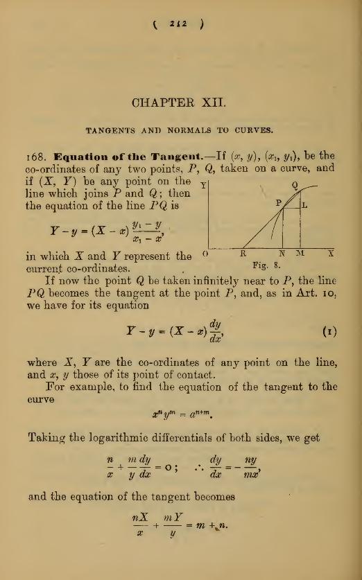
{ *l* )
CHAPTER XII.
TANGENTS AND NORMALS TO CURVES.
1 68. Equation of the Tangent.—If (a?, y)> [x X9 y x), be the
co-ordinates of any two points, P, Q, taken on a curve, and
if (X, Y) be any point on the Yline which joins P and Q ; then
the equation of the line PQ is
in which X and Y represent the ° R n mcurrent co-ordinates. ,
FlS" 8 *
If now the point Q be taken infinitely near to P, the line
PQ becomes the tangent at the point P, and, as in Art. 10,
we have for its equation
r- y -(X-*>| ()
where X, Y are the co-ordinates of any point on the line,
and xy y those of its point of contact.
For example, to find the equation of the tangent to the
curve
Taking the logarithmic differentials of both sides, we get
nyn mdyx y ax
dy
dx mx
and the equation of the tangent becomes
nX mY— +x y
= m +vw.

Tangents Parallel to a Given Line. 2 1
3
_ _ _ . _ . m + nIf we make X= o, and T= o, separately, we get ymtn ~\~ n
and x for the lengths of the intercepts made by the
tangent on the axes of x and y, respectively. This result
furnishes an easy geometrical method of drawing the tangent
at any point on a curve of this class.
If m = 1, n = 1, the preceding equation represents a
hyperbola ; if m = 2, and n = - 1, it represents a parabola.
169. If the equation of the curve be of the form
f(xy y) - o, and if f(x> y) be denoted by u9we have from
Art. 100,
du
dym Jdx
dx duJ
dy
and hence the equation of the tangent becomes
du dulx--) 5+.<r-r)^-a (
2)
The points on the curve at which the tangents are
duparallel to the axis of x must satisfy the equation — = o
;
axthey are accordingly given by the intersection of the curve,
u = o, with the curve whose equation is — = o. The y co-ax
ordinates at such points are evidently in general either
maxima or minima.Similar remarks apply to the points at which the tangents
are parallel to the axis of y.
To find the tangents parallel to the line y = mx + «. Thepoints of contact must evidently satisfy
du du— + m-r =0.dx dy
The points of intersection of the curve represented by

214 Tangents and Normals to Curves.
t
this equation with the given curve are the points of contact
of the system of parallel tangents in question.
The results in this and the preceding Article evidently
apply to oblique as well as to rectangular axes.
Examples.
I. To find the equation of the tangent to the ellipse
a2+
b2
du 2x du iyHere -r- = -«-> -j~ = ii"»dx a2 dy b2
and the required equation is
$(*-.) + J<r-if)-*
xX yY x2 y2
a* o* a2 b2
2. Find tue equation of the tangent at any point on the curve
#m ym Xxm~ l Tyml— + — = i. Ans. + -|— = I.am bm am om
3. If two curves, whose equations are denoted by u - o, u' = o, intersect in
a point (x, y), and if « be their angle of intersection, prove that
du du* du' du
._ dxdydxdydu du* du du**
dx dx dy dy
4. Hence, if the curves intersect at right angles, we must have
du du' du du' _dx dx dy dy
5. Apply this to find the condition that the curves
x2 y2 x2 y2
jnould intersect at right angles. Ans. a2 - b* = a'2 - b' 2.

Equation of Normal. 215
1 70. Equation of formal.—Since the normal at anypoint on a curve is perpendicular to the tangent, its equation,
when the co-ordinate axes are rectangular, is
ordu du_(F- y)=--(X-*). (3)
The points at which normals are parallel to the line
y = mx + n are given by aid of the equation of the curve u = o
along with the equation
du
Ty— = m
du
Examples.
1. Find the equation of the normal at any point (xf y) on the ellipse
-s +b*= l
A a*X FYAns. — a 1 - b%
.
x y
2, Find the equation of the normal at any point on the curve
y"» = ax1*. Ans. nYy + mXx = ny3 + mx2.
171. Subtange nt and Nu s> nor inal.—In the accom-panying figure, let PT repre- ysent the tangent at the point P,Pi^the normal; OM, PM the
co-ordinates at P ; then the
lines TN and DIN are called
the subtangent and subnormal o"
corresponding to the point P. Fig. 9.
To find the expressions for their lengths, let <p = L PTM>
thenPMTM
MN
tand>=^; .\ Tif=|-,r dx dy
da
4d» MN =y%

216 Tangents and Normals to Curves.
The lengths of PT and PN are sometimes called the
lengths of the tangent and the normal at P : it is easily
seen that
-Htl-PN-V.X+ -r- . PT =jfWidy
dx
Examples.
i. To find the length of the subnormal in the ellipse
»»+
** '•
dy V1 .
Here '*—?*'
the negative sign signifies that MN is measured from M in the negative
direction along the axis of x> i.e. the point N lies between M and the centre \
as is also evident from the 6hape of the curve.
2. Prove that the subtangent in the logarithmic curve, y = a*, is of constant
length.
3. Prove that the subnormal in the parabola, y2 = imx, is equal to m.
4. Find the length of the part of the normal to the catenary
. X X.
y*intercepted by the axis of x. <dns. —
.
5. Find at what point the subtangent to the curve whose equation is
xy2 = a2 (a -~ x)
ais a maximum. Ans. x = -, y - a.
172. Perpendicular on Tangent.—Let p be the length
of the perpendicular from the origin on the tangent at anypoint on the curve
F{x, y) = c,

Length of Perpendicular on Tangent. 217
then the equation of the tangent may be written
X 00s to + T sin to = p>
where a> is the angle which the perpendicular makes with
the axis of x.
Denoting F(x, y) by u, and comparing this form of the
equation with that in (2), and representing the common value
of the fraction by A,
du du du du
dx dy dx dy xwe get = --£— = 2= A.00s to sin to p
*-{£)<%)'du dux— +y —
and p=k
** * -.(4)
iftY~ (—Y
W«ACor. If jF(#, ^) be a homogeneous expression of thedegree in x andy, then by Euler's formula, Art. 102, we have
du duX ~T + y^- = nu = nc,dx * dy '
and the expression for the length of the perpendicularbecomes in this case
4\dx)+\dy)
173. In the curve
of" ym
to prove that
m
pm~ l - {a cos a;)™-1 + (b sin w)m~\ (5)

2 1
8
Tangents and Normals to Curves.
By Ex. 2, Art. 169, the equation of the tangent is
Xxm~' Yyrh~ l
am4 ~W * ! ;
comparing this with the form
X cos o) 4 JT sin o> = jt>,
we getcos a) _ xnt~ l sin io ym
~x
p am9 p bm
or
1 1
sin w\m_1y(a cos w\m~l_x (b sin
\ P J ~* \ V
Hence, substituting in the equation of the curve, we obtain
the result required.
1 74. Locus of Foot of Perpendicular for the sameCurve.—Let X, Y be the co- ordinates of the point in ques-
X Ytion, and we have, evidently, cos w *= — , sin <o = — : substi-
tuting these values for cos a; and sin i* in (5), it becomes
(X2 + F2)^1 = (aX)m-1» (b Y)m"\
since p2 = X 2 + F2
.
175. Another Form of the Equation to a Tan-gent.—If the equation of a curve of the n th degree be
written in the form
<j)(x, y) = un + un.i + un„2 + . . . - t#3 + ty + tt - o,
where ww denotes the homogeneous part of the nth degree in
the equation, ^fw_ 1 that of the (n - i)th
9&o. ; then, by Oor.
Art. 103, we have
dx dy

Number of Tangents from an External Point. 219
Hence the equation of the tangent in Art. 169 becomes
X-~ + T -f- + un^ 4- 2uM + . . . -f nu<> = o; (6)
dx dy
an equation of the (n - i)th degree in x and y.
176. Number of Tangents from an ExternalPoint.—To find the number of tangents which can be
drawn to a curve of the nth degree from a point (a, |3), we sub-
stitute a for X, and |3 for Fin (6), and it becomes
dtp dq> .
a j- + /3 j- + ttn-i + 2^n_2 + • • • + nU = O. (7)
This represents a curve of the (n - i)th degree in x and y,
and the points of its intersection with the given curve are the
points of contact of all the tangents which can be drawnfrom the point (a, j3) to the curve. Moreover, as two curves
of the degrees n and n - i intersect in general in n (n - i)
points, real or imaginary (Salmon's Conie Sections, Art. 2 $8),
it follows that there can in general be n(n - 1) real or
imaginary tangents drawn from an external point to a curve
of the nth degree.
If the curve be of the second degree, equation (7) be-
comesd<b ~d<b
a -y- + B -7- 4- t«i + 2U = O,dx ' dy
an equation of the first degree, which evidently represents
the polar of (a, j3) with respect to the conic.
In the curve of the third degree
w8 + u2 + u x + u = o,
equation (7) becomes
dd> d<p
which represents a conic that passes through the points of
contact of the tangents to the curve from the point (a, |3).
This conic is called the polar conic of the point. For theorigin it becomes
U% + 2Ui j $uQ= o.

220 Tangents and Normals to Curves.
177. Number of Normals which pass through aGiven Point.—If a normal pass through the point (a, j3),
we must have from (3),
,du du*-•> ;§?-»-*>
»
This represents a curve of the nth degree, which intersects the
given curve in general in n2 points, real or imaginary, the
normals at which all pass through the point (a, /3).
For example, the points on the ellipse
a2+V '
at which the normals pass through a given point (a, /3),
are determined by the intersection of the ellipse with the
hyperbolaxy{a2 - b
2) - a2 ay - b
2fix.
For the modification in the results of this and the pre-
ceding article arising from the existence of singular points on
the curve, the student is referred to Salmon's Higher Plane
Curves, Arts. 66, 67, m.178. Differential of the Are of a Plane Curve.
Direction of the Tangent.—If the length of the aro of a
curve, measured from a fixed point A on it, be denoted by s,
then an infinitely small portion of it is represented by ds.
Again, if <j>' represent the angle QPL (fig. 8), we have
, PL , . , QLcos <p = -p^, and sin <p = p^ 5
but in the limit, PL = dx, QL = dy, and PQ = ds* and also
<p' becomes PTX, or <p (fig. 9).
* In Art. 37 it has been proved that the difference between the length of an
infinitely small arc and its chord is an infinitely small quantity of the second
arc PQ PQorder in comparison with the length of the chord ; i.e. —
-
is infinitely
small of the second order, and therefore this fraction vanishes in the limit.
Hence J~Fn= l
»ultimately.
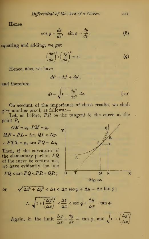
Differential of the Arc of a Carve. 221
Hence
dx dycos* = -, sin = -;
squaring and adding, we get
(%m-Hence, also, we have
ds* = da? + dy\
(8)
(9)
and therefore
dsF dtf
dx2dx. (iot
On account of the importance of these results, we shall
give another proof, as follows :
—
Let, as before, PR be the tangent to the curve at the
point P,
OM=x, PM=y,MN=PL = Ax, QL = Ay.
L PTX = 0, arc PQ = As,
Then, if the curvature of
the elementary portion PQof the curve be continuous,
we have evidently the line
PQ<aroPQ<PR+QR; 6 f M w
Fig. io.
or ^/Ax2 + Ay2 < A« < Ax seo (j> + Ay - Ax tan<f> ;
I /AyY ^ Ay•'• J ! + t^ <T" < sec + tan <p.
V \AxJ Ax Ax
Again, in the limit -~ = -^ = tan </>, and Ji + I—
* A# rfa?T S \Ax

222 Tangents and Normals to Curves.
becomes / 1 + ( -j-)or sec <p , accordingly each of the pre-
ceding expressions converges to the same limiting value, and
we have — = / 1 + ( -7- ; which establishes the required
result.
179. Polar Co-ordinates.—The position of any point
in a plane is determined when its distance from a fixed point
called a pole, and the angle which that distance makes with a
fixed line, are known ; these are called the polar co-ordinates
of the point, and are usually denoted by the letters r and f).
The fixed line is called the prime rector, and r is called the
radius rector of the point.
The equation of a curve referred to polar co-ordinates is
generally written in one or other of the forms,
r = /(0), ori^(r, 0) =0,
according as r is given explicitly or implicitly in terms of 0.
Also, if be positive when measured above the prime vector,
it must be regarded as negative when measured below it.
180. Angle between Tangent and Radius Veetor.
Let be the pole, P and Q two nearpoints on the curve, PM a perpendicular
on OQ, OP = r, POX = 0, and + the
angle between the tangent and radius
vector. Then„_ PM . „„ PMtanOQP=--, sin OOP =_,
QMcos OQP = —r : but in the limit whenQP Fig. 11.
Q and P coincide, the angle OQPbecomes equal to \p, and*
QM dr PM rdO AtS7\
= T) -^7^ = —r> at the same time ;PQ ds PQ ds
,*
1rdd
4. 1rde
1 \or cos 4> = —, sm \l> = •— , tan \L = -=-, (11)ate <& rfr
v
These results can be easily established from Art. 37.
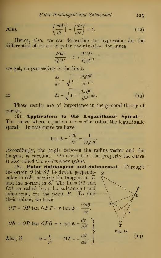
Polar Subtangent and Subnormal. 223
Also,rdOV
Ts)= I (12)
Hence, also, we can determine an expression for the
differential of an arc in polar co-ordinates ; for, since
PQ PM'QM 2
"
QJ["
we get, on proceeding to the limit,
daj
dr=V
rW1 +
d,.2 >
or ds = 1 + —r-=- dr.dr (13)
These results are of importance in the general theory of
curves.
181. Application to the Logarithmic Spiral.—The curve whose equation is r = a9 is called the logarithmic
spiral. In this curve we have
rdO 1
tan ip - -— = = .
dr log a
Accordingly, the angle between the radius vector and the
tangent is constant. On account of this property the curveis also called the equiangular spiral.
182. Polar Subtangent anil Subnormal.—Throughthe origin let ST be drawn perpendi- g
cular to OP, meeting the tangent in T,
and the normal in & The lines T andOS are called the polar subtangent andsubnormal, for the point P. To find
their values, we have2 7/1
OT = OP tan OPT = r tan $ = ---.
08 = OP tan OPS = r cot $ =
Also, if « = -, OT = -
dr
dr •)
Tff \
dd \
du „
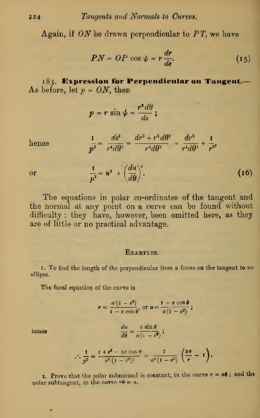
224 Tangents and Normals to Curves.
Again, if ON he drawn perpendicular to PT, we haye
PN = OP cos t/, = rJ. (15)
183. Expression for Perpendicular on Tangent.—As before, let p = ON, then
. , r>d9p = rsin^ =—
;
i_ ds>_ dr2 +rW dr%i_
06 p*~ rW>~ rW %W +r"
or i-"*tsy- <•'f \m
The equations in polar co-ordinates of the tangent andthe normal at any point on a curve can be found without
difficulty : they have, however, been omitted here, as they
are of little or no practical advantage.
Examples.
I. To find the length of the perpendicular from a focus on the tangent to an
ellipse.
The focal equation of the curve is
a(i - e2) 1 - e cos0r = . or w== __ —
;
I -*cos0 a (1 - «»)
du t sin Qhence
d$ a(i -«•)*
1 4- tf2 — ze cos 6
p* a*(i-e2)- a*(i-«2
)\r T
2. Prove that the polar subnormal is constant, in the curve r m aB ;and the
Dolar subtangent, in the ciitva w» = a.
Inverse Carves. 225
184. Inverse Curves.—If on any radius vector OP,drawn from a fixed origin 0, a point P' be taken such that
the rectangle OP . OP" is constant, the point P' is called the
inverse of the point P ; and if P describe any curve, Pf
describes another curve called the inverse of the former.
The polar equation of the inverse is obtained immediately
from that of the original curve byk2
substituting — instead of r in its
equation ; where k2is equal to the
constant OP . OP".
Again, let P, Q be two points,
and P,Q' the inverse points ; then
since OP . 0P; = OQ . OQ', the
four points P, Q, Q', P', lie on a
circle, and hence the triangles
OQP and OP'Q' are equiangular
;
PQ OP OP . OQ OP. OQP'Q' ~ OQ! ~ OQ . OQ' ~ k2
(i7)
Again, if P, Q be infinitely near points, denoting the
lengths of the corresponding elements of the curve and of its
inverse by ds and ds', the preceding result becomes
ds = — ds . (18)
185. Direction of the Tangent to an InverseCurve.—Let the points P, Q belong to one curve, and P', Q'
to its inverse; then when P and Q coincide, the lines PQ,P'Q' become the tangents at the inverse points P and P'
:
again, since the angle SPP' = the angle SQ'Q, it follows that
the tangents at P and P' form an isosceles triangle with the
line PP'.By aid of this property the tangent at any point on a
curve can be drawn, whenever that at the correspondingpoint of the inverse curve is known.
It follows immediately from the preceding result, that if
two carves intersect at any angle, their inverse carves intersect at
the same angle.

226 Tangents and Normals to Curves.
1 86. .Equation to the Inverse of a Given Curve.—Suppose the curve referred to rectangular axes drawn throughthe pole 0, and that # and y are the co-ordinates of a point Pon the curve, X and Y those of the inverse point P/
; then
x 0P_ OP . OF k2.
y_ J?x " op"
=
op"2~~ x2 + r2 ;
similarly y " X 2 + Y2 ;
hence the equation of the inverse is got by substituting
k2x . k2y
anda?2 + y
2 x% + y*
instead of # and y in the equation of the original curve
Again, let the equation of the original curve, as in Art.
174, be
*» + Un_i + Un-2 + . . . 4- U2 + U x + Wo = O.
z*2//, k2/ij
When — and _ _ are substituted for x and y, unx2 + y
2 x2 + y%
k2nubecomes evidently 7-r -rr-*J
(*2+ */
2
)
n
Accordingly, the equation of the inverse curve is
k2nun + k2n-2u^{x2 + y
2) + &2n-%n_2 (#
2 + y2
)
2 + . . .
+ u (x2 + y
2
)
n = o. (19)
For instance, the equation of any right line is of the form
u v + u = o
;
hence that of its inverse with respect to the origin is
k2Ux + u (x
2 + y2) = o.
This represents a cirole passing through the pole, as is
well known, except when u = o ; i.e. when the line passes
through the pole 0.
Again, the equation of the inverse of the circle
x2 + y2 + v x
+ tt = o,
with respect to the origin, is
(A4 + Vih + u (x
2 + if)) (a? + if) = o,
which represents another circle, along with the two imaginaryright lines x2 + y
2 = o.

Pedal Curves. 227
Again, the general equation of a conic is of the form
u% + Ui + tio =» o
;
henoe that of its inverse with respect to the origin is
k*u2 + khh(x2 + y2) + ii (x
2 + y2
)
2=* o,
which represents a curve of the fourth degree of the class
called "bicircular quartics."
If the origin be on the conic the absolute term u vanishes,
and the inverse is the curve of the third degree represented
byk2u2 + Ui (x
2 + y2) = o.
This curve is called a " circular cubic."
If the focus be the origin of inversion, the inverse is a
curve called the Limacon of Pascal. The form of this curve
will be given in a subsequent Chapter.
187. Pedal Curves.—If from any point as origin a per-
pendicular be drawn to the tangent to a given curve, the locus
of the foot of the perpendicular is called the pedal of the curve
with respect to the assumed origin.
In like manner, if perpendiculars be drawn to the tan-
gents to the pedal, we get a new curve called the secondpedalof the original, and so on. With respect to its pedal, the
original curve is styled the first negative pedal, &c.
188. Tangent at any Point to the Pedal of agiven Curve.—Let ON, ON'be the perpendiculars from the
origin on the tangents drawnat two points P and Q on the
given curve, and T the intersec-
tion of these tangents;join NN';
then since the angles ONT andON'T are right angles, the qua-drilateral ONN'T is inscribable
in a cirole,
.-. lON'N= lOTN.
In the limit when P and Q coincide, L OTN = L OPN,and NN' becomes the tangent to the locus of N\ hence the
Q 2

228 Tangents and Normals to Curves.
latter tangent makes the same angle with ON that the
tangent at P makes with OP. This property enables us
to draw the tangent at any point N on the pedal locus in
question.
Again, if j/ represent the perpendicular on the tangent at
iV^ to the first pedal, from similar triangles we evidently have
r -PlVHence, if the equation of a curve be given in the form
p2
r =f(p), that of its first pedal is of the form — = f(p), in
which p and p' are respectively analogous to r and p in theoriginal curve. In like manner the equation of the nextpedal can be determined, and so on.
189. Reciprocal Polars.—If on the perpendicular ONa point P' be taken, such that OP7
. ON is constant (k2 sup-
pose), the point P' is evidently the pole of the line PN withrespect to the circle of radius k and centre ; and if all the
tangents to the curve be taken, the locus of their poles is a
new curve. We shall denote these curves by the letters Aand P, respectively. Again, by elementary geometry, the
point of intersection of any two lines is the pole of the line
joining the poles of the lines * Now, if the lines betaken as
two infinitely near tangents to the curve A, the line joining
their poles becomes a tangent to P ; accordingly, the tangentto the curve P has its pole on the curve A. Hence A is the
locus of the poles of the tangents to P.In consequence of this reciprocal relation, the curves A and
P are called reciprocal polars of each other with respect to the
circle whose radius is k.
Since to every tangent to a curve corresponds a point onits reciprocal polar, it follows that to a number of points in
directum on one curve correspond a number of tangents to its
reciprocal polar, which pass through a common point.
Again, it is evident that the reciprocal polar to any curve
is the inverse to its pedal ivith respect to the origin.
We have seen in Art. 1
7
6 - that the greatest number of tan-
gents from a point to a curve of the nth degree is n (n - 1) ;
* Townsend's Modern Geometry, vol. i., p. 219.

Reciprocal Polars. 229
hence the greatest number of points in which its reciprocal
polar can be cut by a lice is n(n - 1), or the degree of the
reciprocal polar is n(n- /). For the modification in this
result, arising from singular points in the original curve, as
well as for the complete discussion of reciprocal polars, the
student is referred to Salmon's Higher Plane Curves.
As an example of reciprocal polars we shall take the curve
considered in Art. 173.
If r denote the radius vector of the reciprocal polar cor-
responding to the perpendicular p in the proposed curve, wehave
k%
P = -•r
Substituting this value ior p in equation (5), we get
m m mfk
2\m~i m-i. t»-i
I —J
= (a cos (o) *- (0 sin a>) ,
2m n m
or *^ = (axy^" + {byy*-\
which is the equation of the reciprocal polar of the curve re-
presented by the equation
xm vm
In the particular case of the ellipse,
x2 y2
the reciprocal polar has for its equation
** = aV -f by .
The theory of reciprocal polars indicated above admits of
easy generalization. Thus, if we take the poles with respectto any conic section
( U) of all the tangents to a given curveA
ywe shall get a new curve B ; and it can be easily seen, as
before, that the poles of the tangents toB are situated on thecurve A. Hence the curves are said to be reciprocal polarswith respect to the conic U.
It may be added, that if two curves have a common point,

23° Tangents and Normals to Curves.
their reciprocal polars have a common tangent; and if thecurves touch, their reciprocal polars also touch.
For illustrations of the great importance of this " principleof duality," and of reciprocal polars as a method of investi-gation, the student is referred to Salmon's Conies, ch. xv.
"We next proceed to illustrate the preceding by discussinga few elementary properties of the curves which are comprisedunder the equation rm = am cos mO.
190. Pedal and Reciprocal Polar of rm = am oo&mO.We shall commence by finding the Nangle between the radius vector andthe perpendicular on the tangent.
In the accompanying figure we
have tan PON = cot OPN = - —„rdd
Fig. 15.
But m log r = m log a + log (cos mO);
drhence — = - tan mO,
rdd
and accordingly, LPON-^rnQ. (20)
Again, p = ON= r 00s mO^m+l
or rm+1 = amp. (21)
The equation of the pedal, with respect to 0, can be im-mediately found.
For, let lAON = oj, and we have
c*.- (m + i)0.
Also, from (21),(^"-(f)"".
Hence, the equation of the pedal is
m m / v
pmn m am+l cog (J0^!_\ (22 \
\m + 1 /v
On the Curve rm = am cos md. 231
Consequently, the equation of the pedal is got by substi-
tuting: instead of m in the equation of the curve.m + 1
By a like substitution the equation of the second pedal is
easily seen to be
m m n
r2m+l = a2m+i cos .
2W + I
and that of the nth pedal
in^7- mO
rmn+i = amn+, cog # /_)mn + 1
v *
Again, from Art. 184, it is plain that the inverse to the
curve rm = am cos mO, with respect to a circle of radius a}
is
the curve rm cos mO = am .
Again, the reciprocal polar of the proposed, with respect
to the same circle, being the inverse of its pedal, is the curva
rmM cos = am+K (24)m + 1v '
It may be observed that this equation is got by substitut-
ing for m in the original equation.
Accordingly we see that the pedals, inverse curves, andreciprocal polars of the proposed, are all curves whose equa-
tions are of the same form as that of the proposed.
In a subsequent chapter the student will find an additional
discussion of this class of curves, along with illustrations of
their shape for a few particular values of m.
Examples.
1. The equation of a parabola referred to its focus as pole is
r (1 + cos0) = 2a,
to find the relation between r and p.
QHere r* cos - = a\, and consequently p% — ar%
2
a well-known elementary property of the curve.

232 Tangents and Normals to Curves.
2. The equation r2 cos 20 = a2 represents an equilateral hyperbola; provethat pr = a 1
.
3. The equation r3 = a2 cos iB represents a Lemniscate of Bernoulli ; findthe equation connecting^ and r in this case. Ans. rz - a2
p.
4. Find the equation connecting the radius vector and the perpendicular onthe tangent in the Cardioid whose equation is
r - a(i + cos 0). Ans. r3 = lap2.
It is evident that the Cardioid is the inverse of a parabola with respect toits focus ; and the Lemniscate that of an equilateral hyperbola with respect to
its centre. Accordingly, we can easily draw the tangents at any point on either
of these curves by aid of the Theorem of Art. 185.
5. Show, by the method of Art. 188, that the pedal of the parabola, p2 = ar%
with respect to its focus, is the right line p = a.
6. Show that the pedal of the equilateral hyperbola pr = a2 is a Lemniscate.
7. Find the pedal of the circle r2 - lap. Ans. A Cardioid, r3 = lap2 .
191. Expression for PN.—To find the value of th*
intercept between the point of
contact P and the foot N of
the perpendicular from the
origin on the tangent at P.Let p = ON, w = L NOA, >
PN=t; then lNTN'=lNON'- Aw, also SN' = TS sin STN';
SN'•'• TS = -
—
T%T „ A7/ ; but in thesmNON
limit, when PQ is infinitely small, -
—
^r^ - y/ becomes ~,smNON dw
and TS becomes PN or t
;
• *-% w>
Also OF1 = ON* + PN*;
,...-„ + (|Y. (.6)
192. To proYe thai
ds dt . x

Vectorial Co-ordinates. 233
On reference to the last figure we have
ds r ., „PT-TQ dt .. .. „QN'-PN— = limit of -, — = limit 01;
dw £uj> dw Aw
but PT+ TQ- QN' + PN = TN- TJST';
,ds dt _. .. »TN-TN' .. ., .SN niiThence 3 -j- = limit or = limit 01 -— = ON=p\aw aw Aw Aw
This result, which is due to Legendre, is of importance in
the Integral Calculus, in connexion with the rectification of
curves.
dpIf — be substituted for t, the preceding formula becomes
ds d2
p .
This shape of the result is of use in connexion with curva-
ture, as will be seen in a subsequent chapter.
193. Direction of formal in Tectorial Co-ordi-nates.—In some cases the equation of a curve can be
expressed in terms of the distances from two or more fixed
points or foci. Such distances are called vectorial co-ordi-
nates. For instance, if ru r2 denote the distances from twofixed points, the equation rx + r3 = const, represents an ellipse,
and r l- r2 = const., a hyperbola.
Again, the equation
r Y + mr2 = const.
represents a curve called a Cartesian* oval.
Also, the equation
i\r2 = const.
represents an oval of Cassini, and so on.
The direction of the normal at any point of a curve, in
such cases, can be readily obtained by a geometrical con-
struction.
* A discussion ol tne principal properties of Cartesian ovals will be foundin Chapter XX.

234 Tangents and Normals to Curves.
For, let ^^ P
F(ru r2) = const.
be the equation of the curve, where
FxP = rl% FlP~n<then we have Fi
dFdn dFdr2 _drx ds dr2 ds
Now, ifPThe the tangent at P, then, by Art. 1 80, we have
drx dr2— = cos\f/ l9— = cos fa, where fa = l TPFl9 fa = l TPF2 .
TT dFI
dFI I XHence — cos fa + — cos i£2 = o. (29)
dr\ ar2
Again, from any point R on the normal draw RL andRM respectively parallel to F2P and FXP9
and we have
PL : LR = sin RPM : sin RPL = cos fa : - cos ^x
dFm
dFd)\ ' dr2
Accordingly, if we measure on PFX and PF2 lengths
dF dFPL and PIT, which are in the proportion of — to —-, then
clr\ cl)*2
the diagonal of the parallelogram thus formed is the normalrequired.
This result admits of the following generalization :
Let the equation of the curve* be represented by
F(rl9 r2 , r3 , . . . r») = const.,
* The theorem given above is taken from Poinsofs Elements de Statique,
Neuvieme Edition, p. 435. The principle on which it was founded was, how-ever, given by Leibnitz (Journal den Savant, 1693), and was deduced frommechanical considerations. The term resultant is borrowed from Mechanics,and is obtained by the same construction as that for the resultant of a numberof forces acting at the same point. Thus, to find the resultant of a number of
lines Pa, Pb, Pc, Pd, . . . issuing from a point P, we draw through a a right
line aB, equal and parallel to Pb, and in the same direction ; through B, a right
line BG, equal and parallel to Pc, and so on, whatever be the number of lines:
then the line PR, which closes the polygon, is the resultant in question.

Normals in Vectorial Co-ordinates. 235
where rly r2y . . . rn denote the distances from n fixed points.
To draw the normal at any point, we connect the point with
the n fixed points, and on the joining lines measure off
lengths proportional to
dF dF dF dFL . .
*? *? ^'••^' respectlvely;
then the direction of the normal is the resultant of the lines
thus determined.
For, as before, we have
dFdrx dFdr2 dF drn _drx ds dr2 ds * * * drn ds
tt dF , dF . dF, , .
Hence — cos ypx + — cos \p2 + . . . — cos \pn = o. (30)dr\ ar2 ar^
dF , dF , dF-oos^, -cos*,, ... -Now, — COS 1//1, — cos \p2 , . . . — COS t//n,
are evidently proportional to the projections on the tangent
of the segments measured off in our construction. Moreover,in any polygon, the projection of one side on any right line
is manifestly equal to the sum of the projections of all the
other sides on the same line, taken with their proper signs.
Consequently, from (30), the projection of the resultant onthe tangent is zero ; and, accordingly, the resultant is normalto the curve, which establishes the theorem.
It can be shown without difficulty that the normal at anypoint of a surface whose equation is given in terms of the
distances from fixed points can be determined by the sameconstruction.
Examples.
1. A Cartesian oval is the locus of a point, P, such that its distances, PM,PM\ from the circumferences of two given circles are to each other in a constantratio
;prove geometrically that the tangents to the oval at P, and to the circles
at M and M', meet in the same point.
2. The equation of an ellipse ol Cassini is r/ = abfwhere r and / are the
distances of any point P on the curve, from two fixed points, A and B. Ifbe the middle point of AB, and PiVthe normal at P, prove that L APO= I BPN.
3. In the curve represented by the equation rfi + r2z = a3
,prove that the
normal divides the distance between the foci in the ratio of r2 to n.

236 Tangents and Normals to Curves.
194. In like manner, if the equation of a curve be given
in terms of the angles 0i, 2 , . . . &», which the vectors drawnto fixed points make respectively with a fixed right line, the
direction of the tangent at any point is obtained by an analo-
gous construction.
For, let the equation be represented by
F(0i 9 2, . . . n) = const
Then, by differentiation, we have
dFdOi dFdOz dF dOn .
dQ x ds d0 2 ds ' ddn ds
Hence, as before, from Art. 1 80, we get
1 dF . , 1 dF . , 1 dF .'
^«-m* +^«m^"- +^« Bin * ," a (3I)
Accordingly, if we measure on the lines drawn to the fixed
points segments proportional to
i_dF \_dF \_clF
rx Wi9 n dOJ " * rn dOn
'
and construct the resultant line as before, then this line will
be the tangent required. The proof is identical with that of
last Article.
195. Curves Symmetrical with respect to a Line,and Centres of Curves.—It may be observed here, that
if the equation of a curve be unaltered when y is changed
into - y> then to every value of x correspond equal and oppo-
site values of y\ and, when the co-ordinate axes are rect-
angular, the curve is symmetrical with respect to the axis of x.
In like manner, a curve is symmetrical with respect to
the axis of y, if its equation remains unaltered when the sign
of x is changed.
Again, if, when we change x and y into - x and - y, re-
spectively, the equation of a curve remains unaltered, then
every right line drawn through the origin and terminated bythe curve is divided into equal parts at the origin. This
takes place for a curve of an even degree when the sum of

Symmetrical Curves and Centres. 237
the indices of x and y in each term is even ; and for a curveof an odd degree when the like sum is odd. Such a point is
called the centre* of the curve. For instance, in conies, whenthe equation is of the form
ax2 + 2/ixy + by2 = cy
the origin is a centre. Also, if the equation of a cubicf bereducible to the form
th + u x= o,
the origin is a centre, and every line drawn through it is bi-
sected at that point.
Thus we see that when a cubic has a centre, that pointlies on the curve. This property holds for all curves of anodd degree.
It should be observed that curves of higher degrees thanthe second cannot generally have a centre, for it is evidentlyimpossible by transformation of co-ordinates to eliminate therequisite number of terms from the equation of the curve.For instance, to seek whether a cubic has a centre, we substi-
tute X + a for x, and Y + j3 for y> in its equation, and equateto zero the^ coefficients of X\ XFand F 2
, as well as the abso-lute term, in the new equation : as we have but two arbitraryconstants (a and j3) to satisfy four equations, there will betwo equations of condition among its constants in order thatthe cubic should have a centre. The number of conditions is
obviously greater for curves of higher degrees.
* For a general meaning of the word "centre," as applied to curves ofhigher degrees, see Chasles's Apercu Historique, p. 233, note.
t This name has been given to curves of the third degree by Dr. Salmon,in his Higher Plane Curves, and has been generally adopted by subsequentwriters on the subject.

238 Examples,
Examples.
1. Find the lengths of the subtangect and subnormal at any point of thecurve
pn = an-iz. Arts, nx, —
.
nx
2. Find the subtangent to the curve
nxx*"yn = am4n. Ans. .
m
3. Find the equation of the tangent to the curve
x6 = a3 v8. Ans, = 3.
x y
4. Show that the points of contact of tangents from a point (a, j8) to the
curve
xm yn ~ am+*
ire situated on the hyperbola (m + n) xy - n(3x + may.
5. In the same curve prove that the portion of the tangent intercepted be-
tween the axes is divided at its point of contact into segments which are to eachother in a constant ratio.
6. Find the equation of the tangent at any point to the hypocycloid, #i + ifl
- at ; and prove that the portion of the tangent intercepted between the axes is
of constant length.
7. In the curve x* + yn = an, find the length of the perpendicular drawnfrom the origin to the tangent at any point, and find also the intercept made bythe axes on the tangent.
«nt a2»
Ans. p = — ; intercept
8. If the co-ordinates of every point on a curve satisfy the equations
x - c sin 20(i + cos 2d), y = e cos 20(1 - cos 20),
prove that the tangent at any point makes the angle with the axis of x.
9. The co-ordinates of any point in the cycloid satisfy the equations
x = a(d -sin0), y = a(i-cos0):
prove that the angle which the tangent at the point makes with the axis of y.
is -.2
Examples. 239
H*r* -j- = -r- = cot -.dx ax 2
10. Prove that the locus of the foot of the perpendicular from the pole 01?
the tangent to an equiangular spiral is the same curve turned through an angle.
1 1
.
Prove that the reciprocal polar, with respect to the origin, of an equi-
angular spiral is another spiral equal to the original one.
is. An equiangular spiral touches two given lines at two given points; prove
that the locus of its pole is a circle.
13. Find the equation of the reciprocal polar of the curve
. er* cos - = a*,
3
with respect to a circle with radius a. Ans. The Cardioid H = a\ cos -.
14. Find the equation of the inverse of a conic, the focus being the pole of
inversion.
15. Apply Art. 184, to prove that the equation of the inverse of an ellipse
with respect to any origin is of the form
lap = OFi . pi + OF2 . P2,
fcrhere F\ and F2 are the foci, and />, pi, 02 represent the distances of any point
on the curve from the points 0, f\ and /j, respectively ; f\ and f% being thepoints inverse to the foci, F\ and F2.
16. The equation of a Cartesian oval is of the form
r + kr* = a,
where r and r' are the distances of any point on the curve from two fixed points,
and a, h are constants. Prove that the equation of its inverse, with respect to
any origin, is of the form
api + £02 + 7^8 = o,
where pi, f>2, p3 are the distances of any point on the curve from three fixedpoints, and a, #, y are constants.
17. In general prove that the inverse of the curve
api + &po + 7P3 = o,
with respect to any origin, is another curve whose equation is of similar form.
18. If the radius vector, OP, drawn from the origin to any point Pona

240 Examples.
curve be produced to Pi, until PPi be a constant length ; prove that the normalat Pi to the locus of Pi, the normal at P to the original curve, and the perpen-dicular at the origin to the line <9P, all pass through the same point.
This follows immediately from the value of the polar subnormal given in
Art. 182.
19. If a constant length measured from the curve be taken on the normals
along a given curve, prove that these lines are also normals to the new curve
which is the locus of their extremities.
x2 y'1
20. In the ellipse -= -t 7- = I, if x — a sin *,a1 ¥
prove that
-_ = a\/ 1 - e2 sin2 4>.
d<p
21. If ds be the element of the arc of the inverse of an ellipse with respect
to its centre, prove that
_ a \/i - e?2 sin 2
d> _,
a2 - A2
ds = & -; t-^t <*<*>» where n = —73 '
b2 I -f n sm'<p bA
22. If o> be the angle which the normal at any point on the ellipse
—I- — = 1 makes with the axis-major, prove thata2 ft
M P da>ds =
<i fi - 2 sin2 co)2
23. Express the differential of an elliptic arc in terms of the semi-axis major,
/, of the confocal hyperbola which passes through the point.
Ans. yj— dft.y a2e2 — ufi
24. In the curve rm = am cos m0, prove that
, m-lds m-— = a sec m md.dd
25. If F(x, y) = o be the equation to any plane curve, and<f>
the angle be-
tween the perpendicular fiom the origin on the tangent and the radius vector to
the point of contact, prove that
tan (p
dF aFdx dy
dF dF{
Xlh^ V dy

( *4« )
CHAPTEE XIII.
ASYMPTOTES.
196. Intersection of a Curve and a Right Line.—Before entering on the subject of this chapter it will be ne-
cessary to consider briefly the general question of the inter-
section of a right line with a curve of the nth degree.
Let the equation of the right line be y = fix + v, and sub-
stitute jxx + v instead of y in the equation of the curve ; thenthe roots of the resulting equation in x represent the abscisses
of the points of section of the line and curve.
Moreover, as this equation is always of the nth degree, it
follows that every right line meets a curve of the nth degree in n
points, real or imaginary, and cannot meet it in more.If two roots in the resulting equation be equal, two of the
points of section become coincident, and the line becomes 9
tangent to the curve.
Again, suppose the equation of the curve written in theform of Art. 175, viz.
:
Wn + U^x -f Un-2 + . - . U2 + Ux + U = O ;
then, since un is a homogeneous function of the nth degree in
x and y9 it can be written in the form #"/<>(- ); similarly\xj
*w = +*fi(A «_* = «r*f,(A &o.
And accordingly, the equation of the curve may be written,
*"/.(-) + *n-1//->
) + <*"/,(-) + &c. = o. (il\X/ \xj \xl
Substituting fi + - for - in this, it becomesx x

242 Asymptotes*
Or, expanding by Taylor's Theorem,
+ &c. = o. (2)
The roots of this equation determine the points of section in
question.
We add a few obvious conclusions from the results arrived
at above :—i°. Every right line must intersect a curve of an odd de-
gree in at least one real point ; for every equation of an odddegree has one real root.
2 . A tangent to a curve of the nth degree cannot meet it
in more than n - 2 points besides its points of contact.
3 . Every tangent to a curve of an odd degree must meetit in one other real point besides its point of contact.
4 . Every tangent to a curve of the third degree meets
the curve in one other real point.
197. Definition of an Asymptote.—An asymptote is
a tangent to a curve in the limiting position when its point
of contact is situated at an infinite distance.
i°. No asymptote to a curve of the nth degree can meet it
in more than n - 2 points distinct from that at infinity.
2 . Each asymptote to a curve of the third degree inter*
sects the curve in one point besides that at infinity.
198. Method of finding the Asymptotes to a Curveof the nth Degree.—If one of the points of section of the
line y = jjlx + v with the curve be at an infinite distance, one
root of equation (2) must be infinite, and accordingly wehave in that* case
/.GO = o. (3)
Again, if two of the roots be infinite, we have in addition
'/.'GO +/1GO = o. (4)
* This can be easily established by aid of the reciprocal equation ; for if we
substitute - for x in equation (2), the resulting equation in z will have one root1
zero wnen its absolute term vanishes, i.e., when /o (/a) = o ; it has two roots
zero when we have in addition v/o'(m) +/i(/a) = o ; and so on.

Method offinding Asymptotes in Cartesian Co-ordinates. 243
Accordingly, when the values of ili and v are determined
so as to satisfy the two preceding equations, the correspond-
ing line
y = jux + v
meets the curve in two points in infinity, and consequently is
an asymptote. (Salmon's Conic Sections, Art. 154.)
Hence, if /l< {be a root of the equation/ (/i) = o, the line
/o (W
is in general an asymptote to the curve.
If yi(/i) = o aud/^u) = o have a common root (jui suppose),
\he corresponding asymptote in general passes through the
origin, and is represented by the equation
y = \ixx.
In this case un and u^i evidently have a common factor.
The exceptional case when /<>'(/*) vanishes at the sametime will be considered in a subsequent Article.
To each root of fo(iu) = o corresponds an asymptote, andaccordingly,* every curve of the nth degree has in general n
asymptotes, real or imaginary.
From the preceding it follows that every line parallel
to an asymptote meets the curve in one point at infinity.
This also is immediately apparent from the geometrical
property that a system of parallel lines may be considered
as meeting in the same point at infinity—a principle intro-
duced by Desargues in the beginning of the seventeenth
century, and which must be regarded as one of the first
important steps in the progress of modern geometry.Cor. No line parallel to an asymptote can meet a curve
of the nth degree in more than (n - 1) points besides that
at infinity.
Since every equation of an odd degree has one real
root, it follows that a curve of an odd degree has one real
* Since foijx) is of the nth degree in /x, unless its highest coefficient vanishes,in which case, ae we shall see, there is an additional asymptote parallel to the axis
tip.
R 2
244 Asymptotes.
asymptote, at least, and has accordingly an infinite branchor branches. Hence, no curve of an odd degree can be a closed
curve.
For instance, no curve of the third degree can be a finite
or closed curve.
The equation / (ju) = o, when multiplied by #*, becomesun = o ; consequently the n right lines, real or imaginary,
represented by this equation, are, in general, parallel to the
asymptotes of the curve under consideration.
In the preceding investigation we have not considered
the case in which a root of / (/u) = o either vanishes or is
infinite ; i.e., where the asymptotes are parallel to either
co-ordinate axis. This case will be treated of separately in 9
subsequent Article.
If all the roots of /o(ju) = o be imaginary the curve
has no real asymptote, and consists of one or more closed
branches.
Examples.
To find the asymptotes to the following curves :—
1. y8 = ax3 + Xs .
Substituting fix + v for y, and equating to zero the coefficients of Xs aud x\
separately, in the resulting equation, we obtain
p? — 1 = o, and 3fi2v = a
;
.-. M = i, * = -;
hence the curve has but one real asymptote, viz.,
a9 - * + r*
2. y* — x* + 2ax2y = b2x2.
Here the equations for determining the asvmptotes are
ji* - I = o, and 4/iV + 2afi = o
;
accordingly, the two real asymptotes are
a ay = x , and y + x + - = O.
2 2
3. x* + p:2y - xy2 - iyz + x2 - ixy + ^ + $x + 5 = o.
* 3 ! 3Am. y + - 4- - = o, y = * + -, y + x «* -.
3 4 4 *

Asymptotes Parallel to Co-ordinate Axes. 245
199. Case in which un = o represents the n Asymp-totes.—If the equation of the curve contain no terms of
the (n - i)th degree, that is, if it be of the form
Un + Un_% + Un^ + &C. . . . + Ux + U = O,
the equations for determining the asymptotes become
fo(fji) = o, and v/o(jjl) = o.
The latter equation gives v = o, unless /o'(ju) vanishes along
with/ (/x), i.e., unless/o (a0 has equal roots.
Hence, in curves whose equations are of the above form,
the n right lines represented by the equation un = o are the
n asymptotes, unless two of these lines are coincident.
This exceptional case will be considered in Art. 203.
The simplest example of the preceding is that of the
hyperbola
ace2 + ihxy + by1 = c>
in which the terms of the second degree represent the asymp-totes (Salmon's Conic Sections, Art. 195).
Examples.
Find the real asymptotes to the curves
1. xy* - x*y = a2 {x + y) + £8. Am. x = o, y = o, x - y - o.
2. yz - x* = a?x. „ y - x = O.
3. xi - y* = a2 *y + b2y%. „ * + y = o, x - y = o.
200. Asymptotes parallel to the Co-ordinateAxes.—Suppose the equation of the curve arranged accord-
ing to powers of x, thus
Oox" + (a xy + b)xn'1 + &o. = o
;
then, if a = o and a xy + b = o, or y = , two of the roots
of the equation in x become infinite ; and consequently theline a xy + b = o is an asymptote.

246 Asymptotes.
In other words, whenever the highest power of x is
wanting in the equation of a curve, the coefficient of the
next highest power equated to zero represents an asymptoteparallel to the axis of x.
If a = o, and b = o, the axis of x is itself an asymptote.If xn and x"" 1 be both wanting, the coefficient of xn
~2re-
presents a pair of asymptotes, real or imaginary, parallel to
the axis of x ; and so on.
In like manner, the asymptotes parallel to the axis of ycan be determined.
Examples.
Find the real asymptotes in the following curves :
—
1
.
y2x - ay2 = xz 4- ax2 4 £3 . Am. x = a, y - x 4- a, y 4- x + a - o.
2. y(x2 - $bx 4- 2b2) = X* - lax2 4- a3 , x = b, x = ib
f y 4- ia = x 4- 3#.
3. x2 y* = a2 (x2 4- y2). £ = ± «> 2/ = ± «•
4. #2y2 = a2 (s2 - y2
). y 4 « = o, y - = o.
5. y2« - y*x = x*. x = a.
201. Parabolic Branches.—Suppose the equation
f (fi) = o has equal roots, then/ '(/zi) vanishes along with/ (^),
and the corresponding value of v found from (5) becomes in-
finite, unless f\(fi) vanish at the same time.
Accordingly, the corresponding asymptote is, in general,
situated altogether at infinity.
The ordinary parabola, whose equation is of the form
{ax + (3y)2 = Ix + my 4- n,
furnishes the simplest example of this case, having the
line at infinity for an asymptote. (Salmon's Conic Sections,
Art. 254.)
Branches of this latter class belonging to a curve are
called parabolic, while branches having a finite asymptote are
called hyperbolic.
202. From the preceding investigation it appears that
the asymptotes to a curve of the nth degree depend, in
general, only on the terms of the nih and the (n - i)th degrees

Parallel Asymptotes. 247
in its equation. Consequently, all curves which have the
same terms of the two highest degrees have generally the samt
asymptotes.
There are, however, exceptions to this rule, one of which
will be considered in the next Article.
203. Parallel Asymptotes.—We shall now consider
the case where /o(ju) - o has a pair of equal roots, each repre-
sented by jlci, and where /i(jui) = o, at the same time.
In this case the coefficients of xn and xn~l in (2) both
vanish independently of v, when 11 = fix ; we accordingly
infer that all lines parallel to the line y = jxvX meet the curve
in two points at infinity, and consequently are, in a certain
sense, asymptotes. There are, however, two lines which are
more properly called by that name ; for, substituting jul x for ju
in (2), the two first terms vanish, as already stated, and the
coefficient of xn~2 becomes
v2
fiTifn) + v/ZOm) +/,&!,).I . 2
Hence, if v x and v2 be the roots of the quadratio
v2
JSM + vfi'M+fM-o), (6)
the lines y = juliX + vi, and y = jjliX + v2,
are a pair of parallel asymptotes, meeting the curve in three
points at infinity.
If the roots of the quadratic be imaginary, the corre-
sponding asymptotes are also imaginary.Again, if the term u^ be wanting in the equation, and
if /o(/x) = o have equal roots, the corresponding asymptotesare given by the quadratic
2—;fo"(fi) +/a(pi) - o.
In order that these asymptotes should be real, it is
necessary that/a (iii) and /<>"(&) should have opposite signs.
There is no difficulty in extending the preceding investi-
gation to the case where(/ (/u) = o has three or more equal
roots.

248 Asymptotes.
Examples.
1. (x + yf (x2 + y2 + xy) = a2
y2 + az (x - y).
Here / (/*) - (1 + ^)2(i+ p + /**), /ifc) = o, /iW--«V*;
accordingly vi = «, V2 = - a,
and the corresponding asymptotes are
y + a; - a = o, and y + # + a = o.
The other asymptotes are evidently imaginary.
a. x2 (x 4- y)2 + 2a#2
(# + y) + 8a2 #y + a3y = o.
Here fM = (I + /*)*, /IW = 2^(1 + p), /2 (M) = 8aV ,
••• Mi - - I, /o"00 - 2, /i'Ou) = 2a, /2 (M1 ) = - 8a*,
and the corresponding asymptotes are
y + x — ia = o, and y + # -f 4a = o.
204. If the equation to a curve of the nth degree be of
ihe form
Xy + ax + |3)0i + 02 = o,
where the highest terms containing # and y in (pi are of the
degree n - I, and those in 2 are of the degree n - 2 at most,
the line
y + cup + /3 « O
is an asymptote to the curve.
For, on substituting - ax - j3 instead of y in the equation,
it is evident that the coefficients of xn and xn~ l both vanish
;
hence, by Art. 198, the line y + ax + /3 = o is an asymptote.
Conversely, it can be readily seen that if y + ax + /3 be anasymptote to a curve of the nth degree its equation admits of
being thrown into the preceding form.
In general, if the equation to a curve of the nth degree
be of the form
(y + a xx + j3i)(y + a 2x + j3») . . . (y + anx + j3„) +tf>
2 = o, (7)

Asymptotes to a Cubic. 249
where <p2 contains no term higher than the degree n - 2, the
lines
y + a vx + /3i = o, y + a2# + j3 2 = o, . . . y + a„# + /3* = o
are the n asymptotes of the curve.
This follows at once as in the case considered at the com-mencement of this Article.
For example, the asymptotes to the curve
®y (# + V + ciij{x + y + a2) + b xx + b2y = o
are evidently the four lines
# = 0, y = o, # + y + #! = o, # + y + tf2 = o
If the curve be of the third degree, <j>2 is of the first, andaccordingly the equation of such a curve, having three real
asymptotes, may be written in the form
[y + a xx + /3i) (y + a2x + j3 2) (y + azx + j33) + lx + /ray + w - o. (8)
Hence we infer that the tfAr^g points in which the asymp-
totes to a cubic meet the curve lie in the same right line, viz.,
lx + my + n = o.
The student will find a short discussion of a cubic withthree real asymptotes in Chapter xvin.
205. To prove that, in general, the distance of a point
in any branch of a curve from the corresponding asymptote
diminishes indefinitely as its distance from the origin increases
indefinitely.
If y + ax + j3 = o be the equation of an asymptote, then,
as in the preceding Article, the equation of the curve may bewritten in the form
(y + ax + |3) (pi = tf>2,
where 2 is at least one degree lower than $ x in x and y.

250 Asymptotes.
Hence y + ax + /3 = —
,
fa
and the perpendicular distance of any point (# , t/o) on thecurve from the line y + a# + /3 = o is
a/i + a2a/ I + o2 WiA
where the suffix denotes that # and y are substituted for 2
and y in the functions <j> x and 2 .
Now, when # and y are taken infinitely great, the valueof the preceding fraction depends, in general, on the termsof the highest degree (in x and y) in <p x and <j>2 ; and since the
degree of <p2 is one lower than that of <j>i, it can be easily
seen by the method of Ex. 7, Art. 89, that the fraction ~
becomes, in general, infinitely small when x and y becomeinfinitely great. Hence, the distance of the line y + ax + j3
from the curve becomes infinitely small at the same time.
It is not considered necessary to go more fully into this
discussion here.
The subject of parabolic and other curvilinear asymptotesis omitted as being unsuited to an elementary treatise.
Moreover, their discussion, unless in some elementary cases,
is both indefinite and unsatisfactory, since it can be easily
seen that if a curve has parabolic branches, the number of its
parabolic asymptotes is generally infinite. The reader whodesires full information on this point, as well as the discussion
of the particular parabolas called osculating, is referred to a
paper by M. Plucker, in Liouville's Journal, vol. i., p. 229.
206. Asymptotes in Polar Co-ordinates.—If a
curve be referred to polar co-ordinates, the directions of its
points at an infinite distance from the origin can be in gene-
ral determined by making r = 00, or u = o, in its equation,
and solving the resulting equation in 0. The position of the
asymptote corresponding to any such value of is obtained
by finding the length of the corresponding polar subtangent,
i.e., by finding the value of — corresponding to u = o.ctu

Asymptotes in Polar Co-ordinates. 251
d()
It should be observed that when — is positive, the asymp-
tote lies above the corresponding radius vector, and whennegative, below it; as is easily seen from Art. 182.
If we suppose the equation of the curve, when arranged
in powers of r, to be
rnM0) + r»-yi(0) + . . . + r/M (0) + /„(0) = o,
the transformed equation in u is
u%(0) + u"~%-i(0) + . . . + 11/(0) +/o (0) = o : (9)
consequently, the directions of the asymptotes are given bythe equation
/•(0)=o. (10)
Again, if we differentiate (9) with respect to 0, it is easily
duBeen that the values of -^ corresponding to u = o are given
by the equation
/m% +/.'(») - * (to
provided that none of the functions
/i(0), /»(0), • • • Me)
become infinite for the values of which satisfy equation (10).
Consequently, if a be a root of the equation/o(0) = o, the
curve has an asymptote making the angle a with the primevector, and whose perpendicular distance from the origin is
i -i i /i(«)represented by - ~£-r.
It is readily seen that the equation of the correspondingasymptote is
This method will be best explained by applyiug it to oneor two elementary Examples.

252 Asymptotes.
Examples.
I. Let the curve be represented by the equation
r = a sec + b tan 0.
COS0Here u m
a -f b sin 0*
tTT1 IT _ , <fo wWhen = -, we have u = o, and — s=
i7
tf0 a + *
Accordingly, the corresponding polar subtangent is a + b, and hence the line
perpendicular to the prime vector at the distance a + b from the origin is anasymptote to the curve.
Again, u vanishes also when = — , and the corresponding value of the
polar subtangent is a — b ; thus giving another asymptote.
2. r = a sec md + £ tan w0.
cos w?0Here u s=
a + £ sin w0
(Vhen =—, we have w = o, and — = ;.2m dd a + V
whence we get one asymptote.
a • -l « 3 71" ,du m
Again, when = — , u = o, and —- = -,&' zm d9 a - b
which gives a second asymptote.
On making - — , we get a third asymptote, and so on.
It may be remarked, that the first, third, . . . asymptotes all touch onefixed circle; and the second, fourth, &c, touch another.
3. Find the equations to the two real asymptotes to the curve
r2 sin(0 - a) + ar sin (0 - 2a) + a2 = o.
Am. r sin (0 - a) = + a sin a.
207. Asymptotic Circles.—In eome curves referred to
polar co-ordinates, when 6 is infinitely great the value of r
tends to a fixed limiting value, and accordingly the curve

Asymptotic Circles. 253
approaches more and more nearly to the circular form at the
same time : in such a case the curve is said to have a circular
asymptote.
For example, in the curve
ad
so long as & is positive r is less than a, a being supposed
positive; but as increases with each revolution, r con-
tinually increases, and tends, after a large number of revo-
lutions, to the limit a ; hence the circle described with the
origin as centre, and radius a, is asymptotic to the curve,
which always lies inside the circle for positive values of 0.
Again, if we assign negative values to 0, similar remarks aro
applicable, and it is easily seen that the same circle is asymp-totic to the corresponding branch of the curve ; with this
difference, that the asymptotic circle lies within the curve in
the latter case, but outside it in the former. The student
will find no difficulty in applying this method to other
curves, such as
ad aO2
_ g (0 + cos0)
'lUanG'r
"2 4a" f " "0 + anfl '

*54 Examples.
Examples.
Find the equations of the real asymptotes to the following curves :
i. y(a2 - x2) = b2 (2x -f e). Ans. y = o, x + a = o, x - a = o.
2. xi - x*y2 + a2 x* + b* = o. * + y = 0, s-y=o, * = o.
3. *4 -*2y2 4*2 + ^8 -«2 =
. s- 1 =0, *+ 1 = 0, x-y = o, x + y = o.
4. (a + *)2(£
2 -s2) = s2
y2. * = o.
5. (a + s)2 (£2 + *») = sy. r = 0> y = x + ^ y + x + a = o.
6. a?>y - 2x2y2 4 #*/3 = a2*2 4 b2y
2. * = o, y = o, * - y = ± a/«*T^".
7. a3 - 4^2 -3#2 + I2a?y _ r2y2 + &r 4 2?/ 4- 4 = o.
-4«j. x + 3 = o, x - iy = o, * + 2y = 6,
8. #2?/* - <wr(tf 4- y)2 - 2a*y2 - a* = o. * - 2* = o, a? f a = o.
9. If the equation to a curve of the third degree be of the form
uz + U\ + w = o,
the lines represented by u$ - o are its asymptotes.
10. If the asymptotes of a cubic be denoted by 0-0, = o, y - of the
equation of the curve may be written in the form
a#7 = AatJ?0 + Cy.
1 1. In the logarithmic curve
X
y = a*,
prove that the negative side of the axis of x is an asymptote.
12. Find the asymptotes to the curve
r cos nd = a.
1 3
.
Find the asymptotes to
r cos md = a cos nB.
14. Show that the curve represented by
#s 4 aby - axy = o
has a parabolic asymptote, x2 4- Ix 4 b 2 = «y.

Examples. 255
15. Find the circular asymptote to the curve
a$ + br — .
+ a
16. Find the condition that the three asymptotes of a cubic should passthrough a common point.
Let the equation of the curve be written in the form
ao + 3*o* + ihy + 3co*2 + &c\xy + $c2y
2 + d x* + sdix2y + $d2xy2 + *%3 = o,
then the condition is
do, d\, d2y
d\, d%, dzyas o.
% 0|, ^2,
This result can he easily arrived at by substituting x + a and y + £ insteadof * and y in the equation of the cubic, and finding the condition that the partof the second degree in the resulting equation should vanish. See Art. 204.
17. When the preceding condition is satisfied show that the co-ordinates,a and £, of the point of intersection of the three asymptotes, are given by theequations
_ C[d\ — Cod2 €odi — cido
dod2 - d{*9
dod2 - d\ 2'
18. If from any point, 0, a right line be drawn meeting a curve of the n**
degree in ifr, Jt2 , . . . Rn , and its asymptotes in n, r2 , . . . rn ,prove that
ORi + OB2 + . . . 0£n = On + Or% + . . . Orn .
N.B.—The terms of the nth and (n — 1)'* degrees are the same for a curveand its asymptotes.
1 9. If a right line be drawn through the point («, 0) parallel to the asymptoteof the cubic (x - a) 3 - x2y = o, prove that the portion of the line intercepted bythe axes is bisected by the curve.
20. If from the origin a right line be drawn parallel to any of the asymptotesof the cubic
y(ax2 + ihxy + by* + 2gx + ify + c) - Xs = o,
show that the portion of this line intercepted between the origin and the linegx +fy + c = o is bisected by the curve.
21. If tangents be drawn to the curve ot? + y3 = a3 from any point on the
line y = x, prove that their points of contact lie on a circle.
22. Show that the asymptotes to the cubic
ax2y + bxy2 + a'x* + by + a"x + b"y = o
are always real, and find their equations.
Am. bx + V - o, ay + a* = o,
ab{ax -t- by) - a2b' - a' b* = o.

( *56 )
CHAPTEE XIV.
MULTIPLE POINTS ON CURVES.
208. In the following elementary discussion of multiple
points of curves the method given by Dr. Salmon in his
Higher Plane Curves has been followed, as being the simplest,
and at the same time the most comprehensive method for
their investigation. The discussion here is to be regarded as
merely introductory to the more general investigation in that
treatise, to which the student is referred for fuller information
on this as well as on the entire theory of curves.
We commence with the general equation of a curve of the
nth degree, which we shall write in the form
<h
+ b<# + b xy
+ C&? + cxxy + cjy*
+ &o. + &o.
+ l<#n + lxx
n'l
y + &o. + lnyn - Of
where the terms are arranged according to their degrees in
ascending order.
When written in the abbreviated form of Art. 1 75, the
preceding equation becomes
W 4- U v + th + • • • + Wn-i + w* = o.
We commence with the equation in its expanded shape,
and suppose the axes rectangular. Transforming to polar

Multiple Points. 257
co-ordinates, by substituting r cos 9 and r sin 9 instead of
x and y, we get
a + {b cos + 6i sin 9) r
+ (c cos2 + Ci cos sin 9 + c2 sin20) r2 + . . .
+ (l cosn 9 + Acos'^fl sinfl + . . . + /n sinM 0)rw = o. (1)
If 9 be considered a constant, the n roots of this equation
in r represent the distances from the origin of the n points
of intersection of the radius vector with the curve.
If a = o, one of these roots is zero for all values of 9 ; as
is also evident since the origin lies on the curve in this case.
A second root will vanish, if, besides a = o, we have
6 cos 9 + b x sin 9 = o. The radius vector in this case meets
the curve in two consecutive points* at the origin, and is
consequently the tangent at that point.
The direction of this tangent is determined by the
equation
K cos 9 + b x sin 9 = o;
accordingly, the equation of the tangent at the origin is
b<& + biy = o.
Hence we conclude that if the absolute term be wantingin the equation of a curve, it passes through the origin, andthe linear part (u x ) in its equation represents the tangent at
that point.
If b = o, the axis of x is a tangent ; if b x= o, the axis
of y is a tangent.
The preceding, as also the subsequent discussion, equally
applies to oblique as to rectangular axes, provided we sub-
stitute mr and nr for x and y ; where
sin (w - 9) . sin 9m =, and n =
;
sin w sin o)
w being the angle between the axes of co-ordinates.
From the preceding, we infer at once that the equation of
the tangent at the origin to the curve
x2(x
1 + y2)= a (x -
y)
* Two points which are infinitely close to each other on the same branch ofa curve are said to he consecutive points on the curve.
S

258 Multiple Points on Curves.
is x - y = o, a line bisecting the internal angle between the
co-ordinate axes. In like manner, the tangent at the origin
can in all cases be immediately determined.
209. Equation of Tangent at any Point.—By aid
of the preceding method the equation of the tangent at anypoint on a curve whose equation is algebraic and rational
can be at once found. For, transferring the origin to that
point, the linear part of the resulting equation represents the
tangent in question.
Thus, if /(.r, y) = o be the equation of the curve, we sub-
stitute X + #, for #, and Y + y x for y, where (#1, y\) is a
point on the curve, and the equation becomes
f(X + zu Y + yx ) = o.
Hence the equation of the tangent referred to the new axes is
xm.rm.c\dx)i \dy)
On substituting x - xl9 and y - y i9 instead of X and Y9we
obtain the equation of the tangent referred to the original
axes, viz.
(«-)I.^-'.)(|),This agrees with the result arrived at in Art. 169.
210. Double Points.—If in the general equation of a
curve we have aQ= 0, b = o, b x
= o, the coefficient of r is
zero for all values of 0, and it follows that all lines drawnthrough the origin meet the curve in two points, coincident
with the origin.
The origin in this case is called a double point.
Moreover, if be such as to satisfy the equation
c cos2 + Cicos sin + c2 sin
2 = 0, (2)
the coefficient of r2 will also disappear, and three roots of
equation (1) will vanish.
As there are two values of tan satisfying equation (2), it
follows that through a double point two lines can be drawn,
each meeting the curve in three coincident points.

Double Points, 259
The equation (2), when multiplied by r2, becomes
c x2 + c xxy + c2y2 = o.
Hence we infer that the lines represented by this equa-
tion connect the double point with consecutive points on the
curve, and are, consequently, tangents to the two branches of
the curve passing through the double point.
Accordingly, when the lowest terms in the equation of a
curve are of the second degree (u2) ythe origin is a double
point, and the equatitm u2 = o represents the pair of tangents at
that point.
For example, let us consider the Lemniscate, whose equa-
tion is
{x2 + y
2
)
2 = a2(x
2 -y2).
On transforming to polar co-ordinates its equation becomes
r4 = a2r2(cos
2 - sin20), or, r2 = a2
cos 2 0.
Now, when = o, r = ± a;
and, if we confine our atten-
tion to the positive values of
r, we see that as increases
IT
from o to -, r diminishes ^4
from a to zero. When 6 > -4
3*-Fig. 18.and <— , r is imaginary, &c,
and it is evident that the figure of the curve is as annexed,having two branches intersecting at the origin, and that the
tangents at that point bisect the angles between the axes.
The equations of these tangents are
x + y = o, and x - y = o,
results which agree with the preceding theory.
211. Nodes, Cusps, and Conjugate Points.*—Thepair of lines represented by u2 = o will be real and distinct,
coincident, or imaginary, according as the roots of equa-
tion (2) are real and unequal, real and equal, or imaginary.
* These have been respectively styled crunodes, spinodes, and acnodes^ byProfessor Cayley. See galraon'g Higher Plane Curves, Art. 38,
S 2
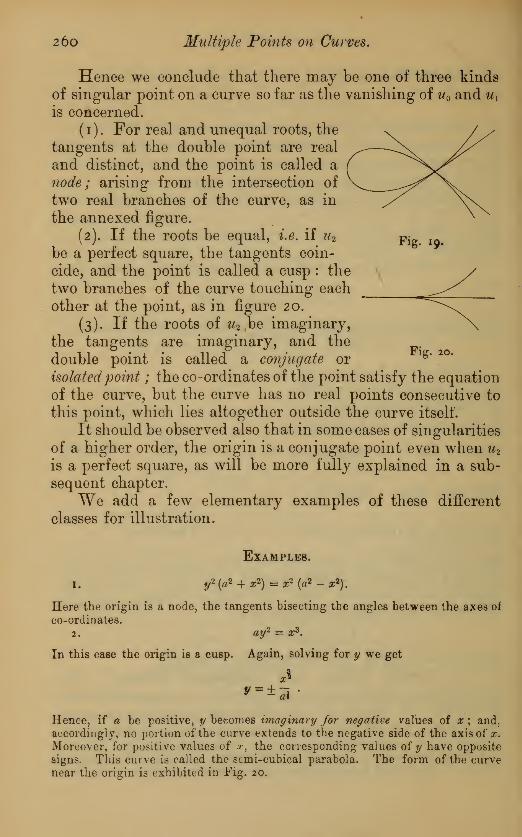
2 tO Multiple Points on Curves.
Fig. 19.
Hence we conclude that there may be one of three kinds
of singular point on a curve so far as the vanishing of u and u{
is concerned.
(1). For real and unequal roots, the
tangents at the double point are real
and distinct, and the point is called a
node; arising from the intersection of
two real branches of the curve, as in
the annexed figure.
(2). If the roots be equal, i.e. if u 2
be a perfect square, the tangents coin-
cide, and the point is called a cusp : the
two branches of the curve touching each
other at the point, as in figure 20.
(3). If the roots of u2 be imaginary,
the tangents are imaginary, and the
double point is called a conjugate or
isolatedpoint ; the co-ordinates of the point satisfy the equation
of the curve, but the curve has no real points consecutive to
this point, which lies altogether outside the curve itself.
It should be observed also that in some cases of singularities
of a higher order, the origin is a conjugate point even when u2
is a perfect square, as will be more fully explained in a sub-
sequent chapter.
We add a few elementary examples of these different
classes for illustration.
Fig. 20.
EXAMPLE8.
1. y2 {a2 + xi
) = x2 {a2 -x2).
Here the origin is a node, the tangents bisecting the angles between the axes of
co-ordinates.
2. ay2 = x3 .
In this case the origin is a cusp. Again, solving for y we get
Hence, if a be positive, y bec.omes imaginary for negative values of x ; and,
accordingly, no portion of the curve extends to the negative side of the axis of x.
Moreover, for positive values of .r, the corresponding values of y have opposite
signs. This curve is called the stmi-cubical parabola. The form of the curve
near the origin is exhibited in Fig. 20.
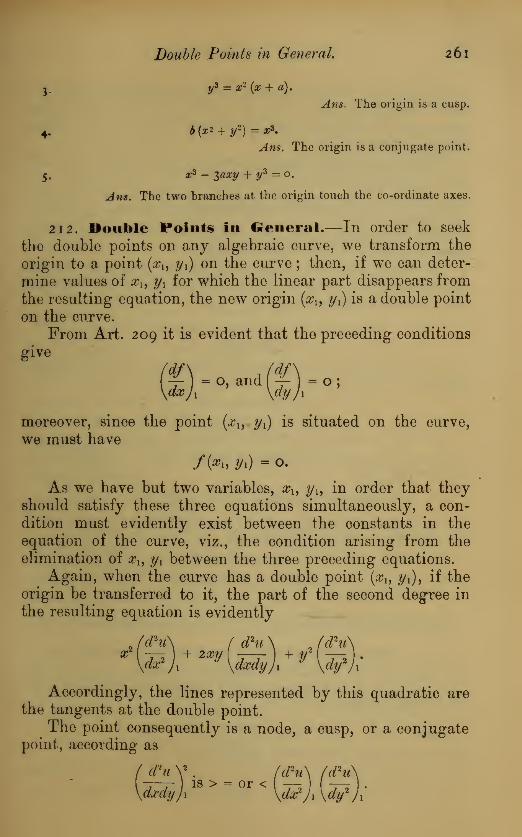
Double Points in General. 261
3. y3 = x2 {x + a).
Ans. The origin is a cusp.
4. |(*t.+ ;)«*.Ans. The origin is a conjugate point.
5. xz - 3<m/ -f y3 = o.
^4w*. The two branches at the origin touch the co-ordinate axes.
212. Double Points in General.—In order to seek
the double points on any algebraic curve, we transform the
origin to a point (xi9 y x ) on the curve ; then, if we can deter-
mine values of x l9 y x for which the linear part disappears from
the resulting equation, the new origin (xl9 y x ) is a double point
on the curve.
From Art. 209 it is evident that the preceding conditions
give
£).=0
'and
(f)ro;
moreover, since the point (x l9 yx ) is situated on the curve,
we must have
As we have but two variables, xl9 y l9 in order that they
should satisfy these three equations simultaneously, a con-
dition must evidently exist between the constants in the
equation of the curve, viz., the condition arising from the
elimination of xl9 y { between the three preceding equations.
Again, when the curve has a double point (xl9 y x ) 9if the
origin be transferred to it, the part of the second degree in
the resulting equation is evidently
Jdhi\ f(Pu\ 2(<Pn\
Accordingly, the lines represented by this quadratic are
the tangents at the double point.
The point consequently is a node, a cusp, or a conjugatepoint, according as
t?u V . (d2u\ fd2u\
^yr >=or<{^)A^l

262 Multiple Points on Curves.
It may be remarked here that no cubic can have morethan one double point ; for if it have two, the line joining
them must be regarded as cutting the curve in four points,
which is impossible.
Again, every line passing through a double point on a cubic
must meet the curve in one, and but one, other point ; ex-
cept the line be a tangent to either branch of the cubic at
the double point, in which case it cannot meet the curve else-
where; the points of section being two consecutive on onebranch, and one on the other branch.
In many cases the existence of double points can be seen
immediately from the equation of the curve. The following
are some easy instances:
—
Examples.
To find the position and nature of the double points in the following
curves :
—
1. (bx - cy) 2 = (x - a) 5.
abThe point x = a
f y = — , is evidently a cusp,c
at which bx - cy = o is the tangent, as in the
accompanying figure
2. (y - c) 2 - (x - ay (x - b).
The point x - a, y = c, is a cusp if a > b, or
if a = b ; but is a conjugate point if a < b.
Fig. 21,
3. y2 = x(x + a) 2
.
The point y = o, # = -#isa conjugate point.
4. x\ \ ift = «i.
The points x = o, y = + a ; and y — o, x = + 0, are easily seen to be cusps.
213. Parabolas of the Third Degree.—The follow-
ing example* will assist the student towards seeing the dis-
tinction, as well as the connexion, between the different kinds
of double points.
Let y1 = {x - a) (x - b) (x - c)
be the equation of a curve, where a< b < c.
* Lacroix, Cal. Dif. t pp. 395-7. Salmon's Higher Plane Curves, Art. 39.

Parabolas of the Third 2)egree. 263
Here y vanishes when x = a, or x = b, or x = c ; accordingly,
if distances OA = a, 05 = J, OG = c, be taken on the axis of
#, the curve passes through the points A, B, and 0.
Moreover, when x < a, y2is negative, and therefore
y is imaginary.
„ x > a, and < 6, y%is positive, and therefore
y is real.
„ x > b, and < c, y2is negative, and therefore
y is imaginary.
„ x > cy y
1is positive, and therefore
y is real ; andincreases indefinitely along with x.
Hence, since the curve is sym-metrical with respect to the axis of
x, it evidently consists of an oval
lying between A and B, and aninfinite branch passing throughC, as in the annexed figure. It
is easily shown that the oval is
not symmetrical with respect to
the perpendicular to AB at its
middle point. Again, if b = c, the
equation becomes
y2 - {x-a)(x- b)
2. Fig. 22.
In this case the point B co-
incides with Cj the oval has
joined the infinite branch, andB has become a double point,
as in the annexed figure.
o
B
X
\Fig. 23.
On the other hand, let b = a9and the equation becomes
y2 = {x -a) 2 {x- c);
in this case the oval has shrunkinto the point A, and the curveis of the annexed form, having qA for a conjugate point.
Next, let a = b = c, and the
equation becomes
y2 = {x-a)*; Pi&- 24 '
A

264 Multiple Points on Curves.
here the points A, B, C, havecome together, and the curve
has a cusp at the points, as in
the annexed figure.
The curves considered in
this Article are called parabolas Fig. 25.
of the third degree.
As an additional example, we shall investigate the fol-
lowing problem :
—
214. Given the three asymptotes of a cubic, to find its equa-
tion, if it have a double point.
Taking two of its asymptotes as axes of co- ordinates, and
supposing the equation of the third to be ax + by + c = o, the
equation of the cubic, by Art. 204, is of the form
xy [ax + by + c) = Ix + my -h n.
Again, the co-ordinates of the double point must satisfy
the equations
du du
or [lax + by + c) y = /, (ax + iby + c) x = m;
from which / and m can be determined when the co-ordinates
of the double point are given.
To find w, we multiply the former equation by x, and the
latter by y, and subtract the sum from three times the equa-
tion of the curve, and thus we get
cxy = zlx + 2my + $n;
from which n can be found.
In the particular case where the double point is a cusp,*
its co-ordinates must satisfy the additional condition
d2u d2u _ f d2u Vdx2 dy2 \dxdyj
'
or [iax + iby + c)2 = qabxy,
and consequently the cusp must lie on the conic represented
by this equation.
* It is essential to notice that the existence of a cusp involves one morerelation among the coefficients of the equation of a curve than in the case of anordinary double point or node.

Double Points on a Cubic. 265
It can be easily seen that this conic* touches at their
middle points the sides of the triangle formed by the asymp-
totes.
The preceding theorem is due to Pliicker,t and is stated
by him as follows :
—
" The locus of the cusps of a system of curves of the third
degree, which have three given lines for asymptotes, is the
maximum ellipse inscribed in the triangle formed by the
given asymptotes."
It can be easily seen that the double point is a node or a
conjugate point, according as it lies outside or inside the
above-mentioDed ellipse.
215. Multiple Points of Higher Curves.—By follow-
ing out the method of Art. 208, the conditions for the existence
of multiple points of higher orders can be readily determined.
Thus, if the lowest terms in the equation of a curve be of
the third degree, the origin is a triple point, and the tangents
to the three branches of the curve at the origin are given bythe equation uz = o.
The different kinds of triple points are distinguished,
according as the lines represented by w3 = o are real anddistinct, coincident, or one real and two imaginary.
In general, if the lowest terms in the equation of a curve
be of the mth degree, the origin is a multiple point of the mih
order, &c.
Again, a point is a triple point on a curve provided that
when the origin is transferred to it the terms below the third
degree disappear from the equation. The co-ordinates of a
triple point consequently must satisfy the equations
du du d2u d2u d2uM =
°' & = °' Ty=
°> ^ =°' ^ =
°' ¥2= °-
Hence in general, for the existence of a triple point on acurve, its coefficients must satisfy four conditions.
The complete investigation of multiple points is effected
* From the form of the equation we see that the lines x = o, y = o aretangents to the conic, and that 2ax + 2by + c = o represents the line joining thepoints of contact ; but this line is parallel to the third asymptote ax + by-\~c = o,
and evidently passes through the middle points of the intercepts made by this
asymptote on the two others.
f Liouvilles Journal, vol. ii. p. 14.
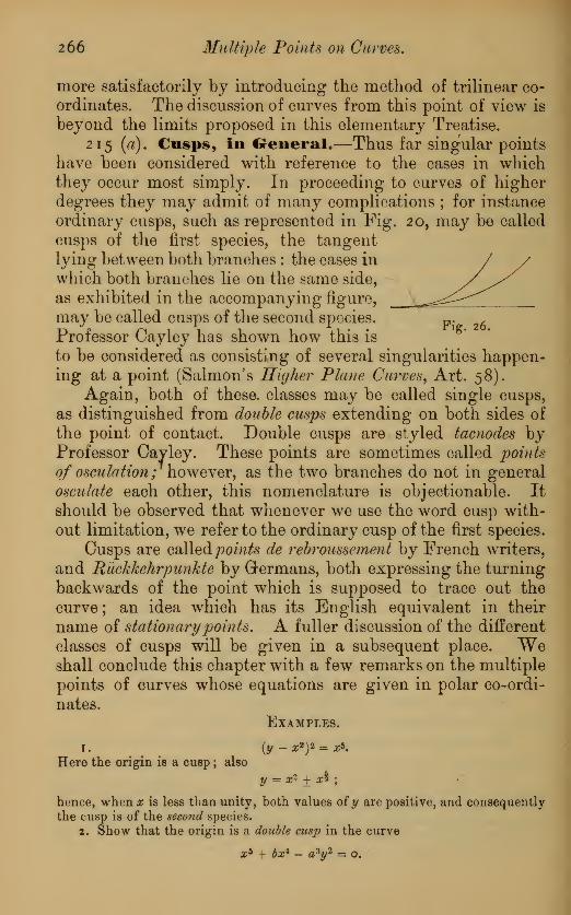
266 Multiple Points on Curves.
more satisfactorily by introducing the method of trilinear co-
ordinates. The discussion of curves from this point of view is
beyond the limits proposed in this elementary Treatise.
215 (a). Cusps, in General.—Thus far singular points
have been considered with reference to the cases in whichthey occur most simply. In proceeding to curves of higher
degrees they may admit of many complications ; for instance
ordinary cusps, such as represented in Fig. 20, may be called
cusps of the first species, the tangentlying between both branches : the cases in
which both branches lie on the same side,
as exhibited in the accompanying figure,
may be called cusps of the second species. „.6
Professor Cayley has shown how this is
to be considered as consisting of several singularities happen-ing at a point (Salmon's Higher Plane Curves, Art. 58).
Again, both of these, classes may be called single cusps,
as distinguished from double cusps extending on both sides of
the point of contact. Double cusps are styled tacnodes byProfessor Cayley. These points are sometimes called points
of osculation
,
'however, as the two branches do not in general
osculate each other, this nomenclature is objectionable. It
should be observed that whenever we use the word cusp with-
out limitation, we refer to the ordinary cusp of the first species.
Cusps are called points de rebroussement by French writers,
and R'uckkehrpunkte by Germans, both expressing the turning
backwards of the point which is supposed to trace out the
curve ; an idea which has its English equivalent in their
name of stationarypoints. A fuller discussion of the different
classes of cusps will be given in a subsequent place. Weshall conclude this chapter with a few remarks on the multiple
points of curves whose equations are given in polar co-ordi-
nates.
Examples.
1. (y ±~ *»)* = *».
Here the origin is a cusp ; also
y = x2 + x%;
hence, when# is less than unity, both values of y are positive, and consequently
the cusp is of the second species.
2. Show that the origin is a double cusp in the curve
xb + bx* - a*y2 = o.
Multiple Points with Polar Co-ordinates. 267
216. multiple Points of Curves in Polar Co-ordi-nates.—If a curve referred to polar co-ordinates pass throughthe origin, it is evident that the direction of the tangent at
that point is found by making r = o in its equation ; in this
case, if the equation of the curve reduce to f(0) = o, the
resulting value of gives the direction of the tangent in
question.
If the equation f(0) = o has two real roots in 0, less than 7r,
the origin is a double point, the tangents being determinedby these values of 0.
If these values of were equal, the origin would be a cusp
;
and so on.
In fact, it will be observed that the multiple points onalgebraic curves have been discussed by reducing them to
polar equations, so that the theory already given must applyto curves referred to polar, as well as to algebraic co-ordi-
nates.
It may be remarked, however, that the order of a multiplepoint cannot, generally, be determined unless with referenceto Cartesian co-ordinates, in like manner as the degree of acurve in general is determined only by a similar reference.
For example, in the equation
r = a cos2 - b sin2
0,
the tangents at the origin are determined by the equation
tan = ± /-, and the origin would seem to be only a double
point ; however, on transforming the equation to rectangularaxes, it becomes
(x2 + fy = (ax2 - by2
)
2
;
from which it appears that the origin is a multiple point of thefourth order, and the curve of the sixth degree. In fact,
what is meant by the degree of a curve, or the multiplicity ofa point, is the number of intersections of the curve with anyright line, or the number of intersections which coincide forevery line through such a point, and neither of these are atonce evident unless the equation be expressed by line co-ordi-nates, such as Cartesian, or trilinear co-ordinates; whereasin polar co-ordinates one of the variables is a circular co-ordinate.

268 Examples.
Examples.
i. Determine the tangents at the origin to the curve
y~ — x2 (i - x2). Ans. x 4 y = o
yx - y - o
2. Show that the curve
x* - l<ixy + y4 = o
touches the axes of co-ordinates at the origin.
3. Find the nature of the origin on the curve
x4 - ax2y 4- by3 = o.
4. Show that the origin is a conjugate point on the curve
ay2 — a? 4- bx2 = o
when a and b have the same sign ; and a node, when they have opposite signs.
5. Show that the origin is a conjugate point on the curve
y2 (x2 - a2 ) = x4
.
6. Prove that the origin is a cusp on the curve
(^ _ x2)2 = x*.
7. In the curve
•(y - x2
)
2 m X»y
show that the origin is a cusp of the first or second species, according as n is
< or > 4.
8. Find the number and the nature of the singular points on the curve
x4, 4- 4ax3 - 2ayz 4- 4a2x2 - T>a2y2 + 4a4 = o.
q. Show that the points of intersection of the curve
er* (!)'
with the axes are cusps.
10. Find the double points on the curve
X4 - qax* 4- <\cr%2 — b2y2
» *b 3y — a4, — b4 -- o.

Examples. 269
11. Prove that the four tangents from the origin to the curve
Ml + Hi + W3 = O
are represented by the equation 4W1 us = u\.
12. Show that to a double point on any curve corresponds another double
point, of the same kind, on the inverse curve with respect to any origin.
13. Prove that the origin in the curve
a4 - iax2y - axy 2 + a ly2 - o
is a cusp of the second species.
14. Show that the cardioid
r = a ( 1 + cos 6)
has a cusp at the origin.
15. If the origin be situated on a curve, prove that its first pedal passes
through the origin, and has a cusp at that point.
16. Find the nature of the origin in the following curves:
—
. • . <*&r3 = «3 sin ;0, rn — aH sin n6, r — .
bQ \ c
17. Show that the origin is a conjugate point on the curve
#* - ax2y + axy2 + a2y2 = o.
18. If the inverse of a conic be taken, show that the origin is a double point
on the inverse curve ; also that the point is a conjugate point for an ellipse, a
cusp for a parabola, and a node for a hyperbola.
19. Show that the condition that the cubic
xy2 + axz + bx2 + ex -I- d + 2ey = o
may have a double point is the same as the condition that the equation
ax* + bx'6 + ex2 + dx - e1 = o
may have equal roots.
20. In the inverse of a curve of the n th degree, show that the origin is a
multiple point of the nth order, and that the n tangents at that point are parallel
to the asymptotes to the original curve.

( *7<> )
CHAPTER XV.
ENVELOPES.
217. method of Envelopes.—If we suppose a series of
different values given to a in the equation
/(*, P> «) = o, (1)
the^i for each value we get a distinct curve, and the above
equation may be regarded as representing an indefinite
number of curves, each of which is determined when the
corresponding value of a is known, and varies as a varies.
The quantity a is called a variable parameter, and the
equation /(#, y, a) = o is said to represent & family of curves;
a single determinate curve corresponding to each distinct
value of a ;provided a enters into the equation in a rational
form only.
If now we regard a as varying continuously, and suppose
the two curves
/(#, y, a) = o, f(x, y, a + Aa) = O
taken, then the co-ordinates of their points of intersection
satisfy each of these equations, and therefore also satisfy the
equation
/(#, ^,a+ Aa) -f{x, y, a)
Aa- O.
Now, in the limit, when Aa is infinitely small, the latter
equation becomes
ffk *">.<,;( 2 )
da
and accordingly the points oi* intersection of two infinitely
near curves of the system satisfy each of tho equations (1)
and (2).

Envelopes. 271
The locus of the points of ultimate intersection for the
entire system of curves represented by /(#, y, a) = o, is ob-
tained by eliminating a between the equations (1) and (2).
This locus is called the envelope of the system, and it can beeasily seen that it is touched by every curve of the system.
For, if we consider three consecutive curves, and suppose
P x to be the point of intersection of the first and second, andP2 that of the second and third, the line Pi P2 joins two infi-
nitely near points on the envelope as well as on the inter-
mediate of the three curves ; and hence is a tangent to each
of these curves.
This result appears also from analytical considerations,
thus :—the direction of the tangent at the point x, y, to the
curve /(a?, y> a) = o, is given by the equation
dx dy dx9
in which a is considered a constant.
Again, if the point x, y be on the envelope, since then a
is given in terms of x and y by equation (2), the direction of
the tangent to the envelope is given by the equation
df df dy df Ida da dy\
dx dy dx da \dx dy dx)
df df dy
dx dy dx
since -j- = o for the point on the envelope.da
Consequently, the values of — are the same for the two(XX
curves at their common point, and hence they have a commontangent at that point.
One or two elementary examples will help to illustrate
this theory.
The equation x cos « + y sin a = />, in which a is a variable
parameter, represents a system of lines situated at the same

272 Envelopes.
perpendicular distance p from the origin, and consequentlyall touching a circle.
This result also follows from the preceding theory ; for
we have
/(^5 //> «) = x °os « + y sin a - p = o,
df (x, y, a)- • = - x sin a + y cos a = O,
and, on eliminating a between these equations, we get
x2 + y2 = jO
2,
which agrees with the result stated above.
Again, to find the envelope of the line
my = aX + —
,
• a
where a is a variable parameter.
Here f(x, y, a) = y - ax - - = o,a »
#/(#, v, a) m fm- -;
}- = -* + - = <>; /. « = /-.
ao a" \ X
Substituting this value for a, we get for the envelope
y1 = imx,
which represents a parabola.
2 1 8. Envelope of La2 + 2Ma + JV= o. Suppose Z, i!f, JV,
to be known functions of x and y, and o a parameter, then
/(#> y, «) = La2 + 2-¥a + i\T = O,
-f-= iLa v iM = o;
da
accordingly, the envelope of the curve represented by the
preceding expression is the curve
LN=M\

Undetermined Multipliers applied to Envelopes. 273
Hence, when L, iff, N are linear functions in x and y>
this envelope is a conic touching the lines L, N, and having
M for the chord of contact.
Conversely, the equation to any tangent to the conic
LN = M 2 can be written in the form
La2 + iMa 4- N= O,*
where a is an arbitrary parameter.
219. Undetermined multipliers applied to Enve-lopes.—In many cases of envelopes the equation of the
moving curve is given in the form
/(*, V, «, /3) - 4f (3)
where the parameters a, /3 are connected by an equation of
the form
(a, /3) = c2 . (4)
In this case we may regard )3 in (3) as a function of a byreason of equation (4) ; hence, differentiating both equations,
the points of intersection of two consecutive curves mustsatisfy the two following equations :
df dfd& jdd> dd> d87 + ^7=0, and-f-
+ -Z-f-
= o.da dp da da dp da
Consequently ' g =||.
da dP
If each of these fractions be equated to the undeterminedquantity A, we get
da da
(5)
•Salmon's Conies, Art. 270.
T

274 Envelopes.
and the required envelope is obtained by eliminating a, |3,and
A between these and the two given equations.
The advantage of this method is especially found whenthe given equations are homogeneous functions in a and ft ;
for suppose them to be of the forms
/{*% v> °> ft) - *• («> P) = *>
where the former is homogeneous of the nth degree, and the
latter of the mth, in a and ft. Multiply the former equation
\n (5) by a, and the latter by ft, and add ; then, by Euler's
theorem of Art. 102, we shall have
nc v= mc2\ or A = —
-, (6)
by means of which value we can generally eliminate a and ft
from our equations.
Examples.
1. To find the envelope of a line of given length {a) whose extremities movealong two fixed rectangular axes.
Taking the given lines for axes of co-ordinates, we have the equations
X V- + ;hI, a* + 0* = a*.a p
Hencex y"1 = ^a > 7ft
= ^&
from which we get1
* = ;*;
.\ a = (a2*)*, = (a>y%
and the required locus is represented by
#t + y\ = at.
2. To find the envelope of a system of concentric and coaxal ellipses of con«
slant area.
x2 y^Here __ + = r , afi = c;
x2yz
hence — = \$, — = Aa ; •• 2A<j = 1
.
or &6
and the required envelope is the equilateral hyperbola
2xy — c.

Examples. 275
3. To find the envelope of all the normals to an ellipse.
Here we have the equations
«*? - & I =# - b\ and -2+ 4* = I,
a £ a2 b2
where a and # are the co-ordinates of any point on the ellipse.
a 2x a b2y BHence, ^ = A
«1' W = ~ &''
consequently \ = a2 - b\
and we get a<x = (a* -b2)a\ fry = - (a2 - b2 )&*;
a / ax \* £( h y
•
' (7" U» - p) ' b
"U* -b 9
)'
Substituting in the equation of the ellipse, we get for the required envelope,
(«b)1+ (%)S=(«2 -£2)!.
This equation represents the evolute of the ellipse.
x y4. Find the envelope of the line - -\— = 1, where a and # are connected by
a £the equation
m mmam + fim _ cm t ^W5. #m+1 -f y
m+1 = Cm+1 .
220. The preceding method can be readily extended to the
general case in which the equation of the enveloping curve
contains any number, n, of variable parameters, which are
connected by n - 1 independent equations. The method of
procedure is the same as that already considered in ChapterXI. on maxima and minima, and does not require a separate
investigation here.
T 2

2j6 Examples.
Examples.
x t/
i. Prove that the envelope of the system of lines - + — = i, where / and mI m
are connected by the equation - + — = i, is the parabolaa o
OH*)'-2. One angle of a triangle is fixed in position, find the envelope of the
opposite side when the area is given. Ans. A hyperbola.
3. Find the envelope of a right line when the sum of the squares of the
perpendiculars on it from two given points is constant.
4. Find the envelope of a right line, when the rectangle under the perpen-
diculars from two given points is constant.
Ans. A conic having the two points as foci.
5. From a point P on the hypothenuse of a right-angled triangle, perpen-
diculars PM, PN are drawn to the sides ; find the envelope of the line MN.6. Find the envelope of the system of circles whose diameters are the chords
drawn parallel to the axis-minor of a given ellipse.
7. Find the envelope of the circle
x% + y2 — 2aex + a2 - b2 = O,
where a is an arbitrary parameter ; and find when the contact between the
circle and the envelope is real, and when imaginary.
(a). Show from this example that the focus of an ellipse may be regarded as
an infinitely small circle having double contact with the ellipse, the directrix
being the chord joining the points of contact.
8. Show that the envelope of the system of conies
x* y2
a a - h
where a is a variable parameter, is represented by the equation
(x ± y/hf + y2 = o.
Hence show that a system of conies having the same foci may be regarded
as inscribed in the same imaginary quadrilateral.
9. Find the envelope of the line
xam -I- t/j8m = «w+1 ,
where the parameters o and 3 are connected by the equation
Ans. xn~m + yn m - I -—
)
n
n-m

Examples, 2JJ
10. On any radius vector of a curve as diameter a circle is described : prove
geometrically that the envelope of all such circles is the first pedal of the curve
with respect to the origin.
1 1. If circles be described on the focal radii vectores of a conic as diameters,
prove that their envelope is the circle described on the axis major of the conic as
diameter.
12. Prove that the envelope of the circles described on the central radii of an
ellipse as diameters is a Lemniscate.
13. Find the envelope of semicircles described on the radii of the curve
r" = an cos nO
as diameters.
14. If perpendiculars be drawn at each point on a curve to the radii vectores
drawn from a given point, prove that their envelope is the reciprocal polar of
the inverse of the given curve, with respect to the given point.
15. Find the envelope of a circle whose centre moves along the circum-
ference of a fixed circle, and which touches a given right line.
16. Ellipses are described with coincident centre and axes, and having the
sum of their semiaxes constant ; find their envelope.
17. Find the equation of the envelope of the line \x + /xy + y = o, wherethe parameters are connected by the equation
a\* + bfi2 + cv2 + ifikv + igv\ + 2h\fi = O.
a, h, g> x
Ans.h, *, /,
*, y, »
,
= 0.
18. At any point of a parabola a line is drawn making with the tangent anangle equal to the angle between the tangent and the ordinate at the point
;
prove that the envelope of the line is the first negative pedal, with regard to the
focus, of the parabola ; and hence that its equation is rl cos - $ = a*, the focus3
being pole.
N.B.—This curve is the caustic by reflexion for rays perpendicular to the
axis of the parabola.
1 9. Join the centre, 0, of an equilateral hyperbola to any point, P, on the
curve, and at P draw a line, PQ, making with the tangent an angle equal to the
angle between OP and the tangent. Show that the envelope of PQ is the first
negative pedal of the curve
r2 = 2a2 sin - $ sin - 0,
3 3
the centre being pole, and axis minor prime vector.
N.B.—This gives the caustic by reflexion of the equilateral hyperbola, thecentre being the radiant point.
20. A right line revolves with a uniform angular velocity, while one of its
points moves uniformly along a fixed right line ; find its envelope.
Ans. A cycloid.

( 2 7 8 )
CHAPTER XVI.
CONVEXITY AND CONCAVITY. POINTS OF INFLEXION.
Fig. 27,
221. Convexity and Concavity.—If the tangent be
drawn at any point on a curve, the neighbouring portion of
the curve generally lies altogether on one side of the tangent,
and is convex with respect to all points lying at the opposite
side of that line, and concave for points at the same side.
Thus, in the accompanying figure, the portion QPQ is
convex towards all points
lying below the tangent, andconcave for points above.
If the curve be referred
to the co-ordinate axes OXand OYy then whenever the
ordinates of points near to
P on the curve are greater
than those of the points on
the tangent corresponding to
the same abscissae, the curve is said to be concave towards
the positive direction of T.
Now, suppose y =<p (x) to be the equation of the curve,
then that of the tangent at a point x, y, by Art. 168, is
r-,-<x-.)g.
Let P be the point x, y, and MN - h = MN\ QN = y x ,
TN = Fi, and we have
y, - *(* + A) = <p(x) + htf(x) +— f(x) + T-r-r^O*) + &c -
Tx= y + h(f>'{x) = <p(x) + h<p'(x)
;
.-. y, - F, = ~ ?{*) + -^—f» + &c. (!)1 . 2 1.2.3

Points of Inflexion. 279
When h is very small, the sign of the right-hand side of
this equation is the same in general as that of its first term,
and accordingly the sign of i/i - Pi, or of QT, is the same as
that of <p"(x).
Hence, for a point above the axis of #, the curve is convextowards that axis when <p"(x) is positive, and concave whennegative.
We accordingly see that the convexity or concavity at any
point depends on the sigtTof <j>"(x) or —^, at the point.U/X
222. Points of Inflexion.—If, however, <p"(x) =0 at
the point P, we shall have
9i- Yi1.2.3
*'"{*) +2-3-4
<j>"(x) + &c. (*)
Now, provided <l>'"(x) be not zero, yx- Yx changes its sign
with h, i.e. if MN' = MN= h,
and if Q lies above T, the
corresponding point Q' lies
below J", and the portions of
the curve near to P lie at
opposite sides of the tangent,
as in the figure.
Consequently, the tangent
at such a point cuts the curve,
as well as touches it, at its FiS- 28 -
point of contact. Such points on a curve are called points of
inflexion.
Again, if <j>'"(x) as well as <j>"{x) vanish at the point P, weshall have
1 .2 .3 .4r
and, provided <£iv(#) be not zero at the point, y x
- Yx does not
change sign with A, and accordingly the tangent does not
intersect the curve at its point of contact.
Generally, the tangent does or does not cut the curve at
its point of contact, according as the first derived function
which does not vanish is of an odd, or of an even order ; as
pan be easily seen by the preceding method,

280 Points of Inflexion,
From the foregoing discussion it follows that at a pointof inflexion the curve changes from convex to concave withrespect to the axis of z, or conversely.
On this account such points are called points of contraryflexure or of inflexion.
223 The subject of inflexion admits also of being treatedby the method of Art. 196, as follows :—The points of in-
tersection of the line?/ = jux + v with the curve y = <j>(x) areevidently determined by the equation
0(*) = fix + v. (3)
Suppose A, B, (7, D, &c, to represent the points of section in
question, and let xXi x2 , . . . xnbe the roots of equation (3) ; ,^~~~^v——^then the line becomes a /p n.
tangent, if two of these ^
roots are equal, i.e., if Fis- 2 9-
<t>'(xi) = jut, where xxdenotes the value of x belonging to the
point of contact.
Again, three of the roots become equal if we have in
addition 0"(#i) = o ; in this case the tangent meets the curve
in three consecutive points, and evidently cuts the curve at its
point of contact ; for in our figure the portions PA and CDof the curve lie at opposite sides of the cutting line, butwhen the points A, B, G become coincident, the portions ABand BC become evanescent, and the curve is evidently cut as
well as touched by the line.
In like manner, if 0"'(#i) also vanish, the tangent mustbe regarded as cutting the curve in four consecutive points :
such a point is called & point of undulation.
It may be observed, that if a right line cut a continuous
branch of a curve in three points, A, B, C, as in our figure,
the curve must change from convex to concave, or conversely,
between the extreme points A and (7, and consequently it
must have a point of inflexion between these points ; and so
on for additional points of section.
Again, the tangent to a curve of the 11th degree at a point of
inflexion cannot intersect the curve in more than n - 3 other
points : for the point of inflexion counts for three amongthe points of section. For example, the tangent to a curve

Harmonic Polar of a Point of Inflexion on a Cubic. 281
of the third degree at a point of inflexion cannot meet the
curve in any other point. Consequently, if a point of in-
flexion on a cubic be taken as origin, and the tangent at it
as axis of xythe equation of the curve must be of the form
<r3 +
y<t>= o,
where <p represents an expression of the second and lower
degrees in x and y. For, when y = o, the three roots of the
resulting equation in x must be each zero, as the axis of x
meets the curve in three points coincident with the origin.
The preceding equation is of the form
lh + U2 + Ui = o,
or, when written in full,
xz + y {ax2-f zhxy + by2
) + y (igx + ify + c) = o. (4)
Now, supposing tangents drawn from the origin to the
curve, their points of contact, by Art. 176, lie on the curve
U 2 + 2Ui = o,
i. e. on the curve
igv+fy + c)t/ = o.
The factor y = o corresponds to the tangent at the pointof inflexion, and the other factor gx + fy + c = o passes
through the points of contact of the three other tangents to
the curve.
Hence, we infer that from a point of inflexion on a cubic
but three tangents can be drawn to the curve, and their three
points of contact lie in a right line.
It can be shown that this right line cuts harmonicallyevery radius vector of the curve which passes through thepoint of inflexion.
For, transforming equation (4) to polar co-ordinates, anddividing by r, it becomes of the form
Ar2 + Br+C = o.
If r', r" be the roots of this quadratic, we have
I i ?.
r+
r"- " C
28
2
Points of Inflexion.
Now, if p be the harmonic mean between r and r", this
gives
21 i £ zg cos + 2/ sin— —^ -j- — — _b
p r r (J c
Hence the equation of the locus of the extremities of the
harmonic means is
gx + fy + e = o. Q. i?. D.
This theorem is due to Maclaurin (Be Lin. Geom. Prop.
Gen., Sec. in. Prop. 9).
From this property the line is called the harmonic polar of
the point of inflexion. This line holds a fundamental place
in the general theory of cubics.*
224. Stationary Tangents.—Since the tangent at a
point of inflexion may be regarded as meeting the curve in
three consecutive points, it follows that at such a point the
tangent does not alter its position as its point of contact
passes to the consecutive point, and hence the tangent in this
case is called a stationary tangent.
d 2
yThe equation — = o follows immediately from the last
ax
consideration ; for when the tangent is stationary we must
have -j- = o, where <j>, as in Art. 171, denotes the angleax
which the tangent makes with the axis of x ; but tan = —
,
hence -r-f = o, which is the same condition for a point ofdx2
inflexion as that before arrived at.
* Chasles, Aper$u Historique, note xx. ; Salmon's Higher Plane Curves.
Art, 179.

Examples. 28$
Examples.
1. Show that the origin is a point of inflexion on the curve
a?y '= bxy + cxz + dxA.
2. The origin is a point of inflexion on the cubic MjjUjsof
3. In the curve am 'ly = xm
,
prove that the origin is a point of inflexion if m be greater than 2.
4. In the sybtem of curves
yn = kxm
y
find under what circumstances the origin is (a) a point of inflexion, (b\ a cusp.
5. Find the co-ordinates of the point of inflexion on the curve
lb*x* — $bx2 + a2y = o. Ans. x = b, y =—
.
Or
6. If a curve of an odd degree has a centre, prove that it is a point of
inflexion on the curve.
7. Prove that the origin is a point of undulation on the curve
Mi + Hi + «5 + &c., + un - o.
8. Show that the points of inflexion on curves referred to polar co-ordinates
are determined by aid of the equation
d 2u _ 1
u + —- = o, where u = -.dd2 r
9. In the curve rdm = a, prove that there is a point of inflexion when
= y/m (1 - m).
x10. In the curve y = c sin -, prove that the points in which the curve
ameets the axis of x are all points of inflexion.
11. Show geometrically that to a node on any curve corresponds a line
touching its reciprocal polar in two distinct points ; and to a cusp corresponds apoint of inflexion.

284 Examples.
1 2. If the origin be a point of inflexion on the curve
Ml + u2 * «3 + . . . + un = o,
prove that ui must contain u\ as a factor.
13. Show that the points of inflexion of the cubical parabola
y2 = {x _ ay (x - b)
lie on the line
ix + a = 4b :
and hence prove that if the cubic "has a node, it has no real point of inflexion;
but if it has a conjugate point, it has two real points of inflexion, besides thatat infinity.
14. Prove that the points of inflexion on the curve y2 - x2 (x2 + 2px + q)
are determined by the equation ixz -f 6px2 + 3 (p2 + q) x + 2pq = o.
15. If y2 = f(x) be the equation of a curve, prove that the abscissae of its
points of inflexion satisfy the equation
irwi*-tfw..rw.
16. Show that the maximum and minimum ordinates of the curve
?=#)/"W-(/WPcorrespond to the points of intersection of the curve y
2 —f{x) with the axis
of a;.
17. When y2 =f(z) represents a cubic, prove that the biquadratic in x
which determines its points of inflexion has one, and but one, pair of real roots.
Prove also that the lesser of these roots corresponds to no real point of inflexion,
while the greater corresponds, in general, to two.
18. Prove that the point of inflexion of the cubic
ay3 + ^bxy2 + ~cx2y + dx? -f $ex2 — o
lies in the right line ay + bx - o, and has for its co-ordinates
xa2e _ \abe* = - — , andy= —
,
where O is the same as in Example 32, p. 190.
19. Find the nature of the double point of the curve
y2 =(*- 2)*(*- 5),
and show that the curve has two real points of inflexion, and that they subtend
a right angle at the double point.
20. The co-ordinates of a point on a curve are given in terms. of an angle
by the equations
x = sec3 0, y = tan sec2 ;
prove that there are two finite points of inflexion on the curve, and find the
values of at these points.

( ^85 )
CHAPTER XVII.
RADIUS OF CURVATURE. EVOLUTES. CONTACT. RADII OF
CURVATURE AT A DOUBLE POINT.
225. Curvature. Angle of Contingence.—Every con-
tinuous curve is regarded as having a determinate curvature
at each point, this curvature being greater or less according
as the curve deviates more or less rapidly from the tangent at
the point.
The total curvature of an arc of a plane curve is measuredby the angle through which it is bent between its extremities
—
that is, by the external angle between the tangents at these
points, assuming that the arc in question has no point of in-
flexion on it. This angle is called the angle of contingence of
the arc.
The curvature of a circle is evidently the same at each of
its points.
To compare the curvatures of
different circles, let the arcs ABand ab of two circles be of equal
length, then the total curvatures
of these arcs are measured by the
angles between their tangents, or
by the angles ACB and acb at
their centres : butlg
*3°*
.-,_ , aroAB arc aft 1 1
LACB: l. acb =——— : = ^tf,:— •AC ac AC ac
Consequently, the curvatures of the two circles are to each
other inverselv as their radii ; or the curvature of a circle
varies inversely as its radius.
Also if As represent any arc of a circle of radius r, andA(j> the angle between the tangents at its extremities, we have
Asr =

286 Radius of Curvature.
The curvature of a curve at any point is found by deter-
mining the circle which has the same curvature as that of anindefinitely small elementary arc of the curve taken at the
point.
226. Radius of Curvature.—Let ds denote an infi-
nitely small element ofa curve at a point, d(p the corresponding
angle of contingence expressed in circular measure, then —d<p
evidently represents the radius of the circle which has the
same curvature as that of the given curve at the point.
This radius is called the radius of curvature for the point,
and is usually denoted by the letter p.
To find an expression for p, let the curve be referred to
rectangular axes, and suppose x and y to be the co-ordinates
of the point in question ; then if cf>denote the angle which the
tangent makes with the axis of x, we have
or
tan * -dlJ
. .
dx''
d . tan <p
dx
d2
y
2d(
t>
dx
<?y' dxv
d(j>
Is"
dih dx d<b= —- — = COS <b -j- = cosdx ds dx
P =1
d$
secs(/> _
d2
ydx*
d-y
d?
1
Again,
Hence . « "ft-l—MBU.. (1)
At a point of inflexion —^ = o : accordingly the radius of
curvature at such a point is infinite : this is otherwise evident
since the tangent in this case meets the curve in three conse-
cutive points. (Art. 222.)
Again, as the expression f 1 +(j-J
Ihas always two
values, the one positive and the other negative, while the

Expressions for Radius of Curvature. 287
curve can have in general but one definite circle of curvature
at any point, it is necessary to agree upon which sign is to be
taken. We shall adopt the positive sign, and regard p as
d2y
being positive when j^ is positive ; i. e. when the curve isax
convex at the point with respect to the axis of x.
227. Other Expressions for p.—It is easy to obtain
other forms of expression for the radius of curvature ; thus
by Art. 178 we have
dx . dy
Hence, if the arc be regarded as the independent variable, weget
d<b d2x d<b dl
y
from which, if we square and add, we obtain
I fd<t>V fd2x\ 2 (d 2
y\P ds \ds2
J \ds+ x? •
12
)
Again, the equations dx = cos $ds, dy = sin <£rfs,
dsgive by differentiation (substituting for d<p)
y
(ds)2
. (ds)2
d2x = cos (pd2s - sin <j>-——, <Py = sin <j>d
2s + cos $ -—-. (3)
9 P
Whence, squaring and adding, we obtain
(d2x)
2 + (d2
y)2 = (d
2s)
2 + <*£,
ds2
°r 9y{d'x) 2 + {d2
y)2 - (d*s)
2' W

288 Radius of Curvature.
Again, if the former equation in (3) be multiplied bysin (p y
and the latter by cos 0, we obtain on subtraction,
ds2 ds3
cos <bd2y - sin <bcPx = — , or dxd 2
y - dyd 2x = —
.
9 P
„ (dx2 + dy2)*
Hence = — ——
.
(<>)P dxd2y - dycPx
Kb)
The independent variable is undetermined in formulae (4)
and (5), and may be any quantity of which both x and y are
functions.
For example, in the motion of a particle along a curve,
when the time is taken as the independent variable, we get
from (4) an important result in Mechanics.
Examples.
1. To find the radius of curvature at any point on the parabola x1 = \my.
tt dy d2y /dy\ 2 #2 vHere 2tn-f- = x
yim-Z = 1, i+[/=i+ —-=i+iL
;
dx dx 1 \dxj 4m2 m
2(w 4 y)*
2. Find the radius of curvature in the catenary
Hence the radius of curvature is equal to the part of the normal intercepted
by the axis of ar, but measured in the opposite direction (Ex. 4, Art. 171).
3. In the cubical parabola ^a2y = s8 , we have
dx ' dx2( \dxj ) a6 2a 4x

General Expression for Radius of Curvature 289
X1 v24. To find the radius of curvature in the ellipse -= + — = I.y
a* b*
Let x — a cos<f>,
then y = b sin<f>>
and we have
dx = - a sin <£dty>, //2# = - a cos <f>aty>
2 - a sin<£^<f>.
dy - b cos <pd<p, cPy = - £ gin <f>dty>2 + £ cos <f>d*<p.
Hence by formula (5) we obtain
(«2 sin2 </> + b2 cos*<p)%
ab
5. In the hypoeycloid x\ + y\ = «i, let x = a cos3</>, then y = sin3<f>,
and re-garding <p as the independent variable, we have
<fc = - 3« cos2</> sin <p d<p> d'x = 3a cos <p d<p2(2 sin2 <£ - cos2 </>),
<fy = 30 sin2^> cos </> «ty>, d^y — $a sin <£ d(/>2
( 2 cos2 <£ — sin2<f>) ,
whence
(dx2 i dy2)i = 3« sin(/> cos <|>Gty>, and dxcPy - dyd2x — - 9a2 sin2<f>cos2«/>aty>3
,
from which we obtain
p=- Z{axy)l.
6. Find the radius of curvature at any point of the curve
v
e* — sec g). ,*«., = « «o (?)
.
228. General Expression for Radius of Curva-ture.—The value of p becomes usually difficult of determi-
nation from formula ( 1) whenever y is not given explicitly in
terms of xythat is, when the equation of the curve is of the
form
u -/(#, y) - o.
We proceed to show how the equation for p is to be trans-
formed in this case. Suppose
du du d2u d 2u d 2u
dx dy ' dx2 ' dxdy ' dy2
then, by Art. 100, we have
dx

2 go Radius of Curvature,
Again, differentiating this equation with respect to #,
regarding y as a function of x in consequence of the given
equation, and observing that
d dL dLdy d dM dM dy
dx dx dy dx dx dx dy dx
we obtain
dL dLdy fdM dMdy\dy d 2
y
dx dy dx \ dx dy dx) dx dx2
or A.*%.0%.kZ-~; (6,
whence, on substituting - — for — , we obtain
<£y AM 2 - 2BLM+ CL2
dx2 ~ M*Consequently
{U + M 2)*
p ~ ± AM2 - 2BLM + OLr (7)
Or, on replacing L> M, A, jB, (7, by their values,
f
duV (du\2
\*
dx)+{dyj]
d 2u (duX1 d 2u du du d 2u fduV
dx2 \dy) dxdy dx dy dy2 \dxj
The result in (6) enables us to determine the second diffe-
rential coefficient of an implicit function in general; a process
which is sometimes required in analysis.
229. The Centime of Curvature is the point ofintersection of two Consecutive Normals.—We shall
next proceed to consider the subject from a geometrical
point of view.
As a circle which passes through two infinitely near
points on a curve is said to h^ve contact of the first order with

Newton's Method of Investigating Curvature. 291
the curve, so the circle which passes through three infinitely
near points on a curve is said to have contact of the second
order with it, and is called the circle of curvature, or the
osculating circle at the point.
Again, the centre of the circle which passes through
three points, P, Q, R, is the intersection of the perpendicu-
lars drawn at the middle points of PQ and QR ; but whenP, Q, R become infinitely near points on a curve, the per-
pendiculars become normals, and the centre of the circle
becomes the limiting position of the intersection of two infinitely
near normals to the curve. (Compare Art. 37, note.)
dsFrom this it is easily seen that we obtain — for the length
U(f)
of the radius of the circle in the limit, as before.
230. Newton's method of investigating Radii ofCurvature.—When the equation of the curve is algebraic
and rational it is easy to obtain anexpression for its radius of curvature*
at any point.
For, take the origin at the
point, and the tangent and normalfor co-ordinate axes; let P be a
point on the curve near to 0, anddescribe a circle through P andtouching the axis of x; draw PNperpendicular to OX and produceit to meet the circle in Q ; then we have
ON2 = PN . NQ.
Hence, if x and y be the co-ordinates of P, we get
ON2 x2
NQ =PN y
But when P is infinitely near to 0, NQ becomes 02), the
* This method of finding the radius of curvature is indicated by Newton(Principia, Lib. I., Sect, 1., Lemma xi.), and has been adopted in a more or leymodified form by many subsequent writers.
U 2

292 Radius of Curvature.
diameter of the circle of curvature, and if p be its radius, wehave
x2
2p = limit of — when x is infinitely small.
Again, since the axis of x is the tangent at the origin,
the equation of the curve, by Art. 208, is of the form
b xy = c x2 + 2cxxy + c2y2 + terms of the third and higher degrees
= Coir2
+ ic xxy + c2y2 + uz + ux + &c. (9)
On dividing by y we obtain
01 = C — + 20!# + C2y + — + &C.
^2
Again, when x is infinitely small, — becomes 2p, and
each* of the other terms at the right-hand side becomes infi-
nitely small ; hence
** 2C'
Thus, for example, the radius of curvature at the origin in
the curve
6y = 2x2 + $xy - \y2 + x*
is -, the axes being rectangular.
* We have assumed above that the terms — , — , &c, become evanescenty y
along with x ; this can be readily established as follows :
—
Let ws = our3 -I- &x2y + yxy2 + Sy8,
t*a xPthen - = a- + fix
2 4 yxy + 5y3 ;
y y
x2
each of the terms after the first vanishes with x, while the first becomes a —*,
V
or 2a/>#, which also vanishes with %ywhen p is finite.
Similar reasoning is applicable to the terms, — , &c.
y
Case of Oblique Axes. 293
From the preceding it follows that when the axis of x is
a tangent at the origin, the length of the radius of curvature
at that point is independent of all the coefficients except
those of y and x2.
231. Case of Oblique Axes.—If the co-ordinate axes
be oblique, and intersect at an angle oj, then PQ no longer
passes through the centre of the circle in the limit, but be-
comes the chord of the circle of curvature which makes the
angle w with the tangent ; accordingly, we have in this case
ON2 x2
2p sin w = -=—l = — , in the limit.PN y'
Henoe, in the case of oblique axes, we have
p sinw = —
.
(101r2Cq
V'
If by and c have opposite signs, p is negative ; this
indicates that the centre of curvature lies below the axis of xy
towards the negative side of the axis of y.
The preceding results show that the radius of curvature
at the origin is the same as that of the parabola, b {y = c x2, at
the same point ; and also that the system of curves obtained
by. varying all the coefficients in (9), except those of y andvT
2, have the same osculating circle, in oblique as well as in
rectangular co-ordinates.
Again, as in Art. 2 2^ 9the osculating circle, since it meets
the curve in three consecutive points, cuts the curve at the
point, in general, as well as touches it.
If c = o in the equation of the curve, and ft, be not zero,
the radius of curvature becomes infinite, and the origin is a
point of inflexion. This is also evident from the form of the"
equation, since the axis of x meets the curve in this case in
three consecutive points.
232. In general, the equation of a curve referred to anyrectangular axes, when the origin is on the curve, may bewritten in the form
2bbx + 2b xy = c x2 + 2c vxy + c2y2 + u z + &c.

294 Radius of Curvature.
Here b x + b xy = o is the equation of the tangent at the
origin ; and the length of the perpendicular PN from the
point (#, y) on this tangent is
b x + bxy
vA,2+ b
x
Also, OP2 = x2 + ^2
, and OP2 = 2p . Pi^ in the limit.
Accordingly, we have, when x and y are infinitely small,
i 2PN 2b x + ibxy
9 OP2
(x2 + y
2)</b 2 + b
c x2 + 2c x xy + c2y2 w8
= — * + j- + &c.(x
2 + y2
)yb
(
2 + J,2
(*» + */2
) -/v + ^(since the point x
y 3/ is on the curve).
Again, the terms contained in _
3
, &c, become evanes-x 1 +y2
cent in the limit, as before (see note, Art. 230).
Hence we have
C + 2d- + ca (-
i c x2 + 2da?y + c2y x \ar
But for points infinitely near the origin we have
oQx + b xy = o, or - = - -:X 0\
Substituting this value instead of - in the preceding equation,x
it becomes
1 c V - 2 J< biCi + c2b*
p (V + *.*)»(II)
The student will find no difficulty in showing the identity
of this result with that given in (7).

Radius of Curvature in terms of r and p. 295
233. Radii of Curvature of Inverse Curves.—It
may be convenient to state here that if two curves be inverse
to each other with respect to any origin, their osculating circles
at two inverse points are also inverse to each other with respect
to the same origin.
Tliis property is evident geometrically from the con-
sideration that a circle is determined when three points on
it are given.
Again, since the centres of the two inverse circles are
in directum with the origin, we can construct the centre of
curvature at any point on a curve, when that for the cor-
responding point on the inverse curve is known.Also, if the osculating circle at any point on a curve
pass through the origin, the corresponding point is a point of
inflexion on the inverse curve.
We shall next proceed to establish another expression for
the radius of curvature, which is of extensive application in
curves referred to polar co-ordinates.
234. Radius of Curvature in terms of r and p.—Let PN and PC be the tangentand normal at any point P on a
curve, FN' and FC those at
the infinitely near point F9then
C is the centre of curvature cor-
responding to the point P. Letbe the origin.
Join OC, and let OC = S,
OP -- r, OF = /, ON = p,ON' =p\ CP= CF = P ;
we havethen
Fig. 32.
OC2 = OP2 + CP2 - 2OP.CP. cos OPC,
or S2 = r2 + p
2 - 2pp.
In like manner we have
S2 = r'2 + p'
Subtracting, we get
2pp
r'% - **' = 2f> (p' - p), or — 2p
P -P r + r

2Qb Radius of Curvature.
Hence we havedr p dr , .— = -, or p = r— . (12)dp r
rdp N
'
This formula can also be deduced immediately from Art.
191 : thus
-r* »t dp dp ds dp dp dr . dpr cos i/, = PiNT « J- - -f
— = p -f - p -f— = p cos \P -f ;aw as «w as dr ds dr
dp dr
235. Chord of Curvature through the Origin.—Let y denote half the intercept made on the line OP by the
circle of curvature, and we evidently have
y = P *mOPN = p£=p-±. (13)
This and the preceding formula are of importance when-ever we can express the equation of the curve in terms of the
lines represented by r and^>.
Their use will be illustrated by the following elementary
examples :
—
Examples.
1 . To find the radius of curvature at any point on a parabola.
Taking the focus as pole, the equation of the curve in terms of r and pevidently is p2 = imr.
_ dr pr /2r3 \iHence = r -— = — = [
—) ; also, 7 -p
dp m \ m J
dr p2
as ir.dp m
2. To find the radius of curvature in an ellipse.
Taking the centre as origin, the equation of the curve is
aH2
a2 + b2 -r2 = —-;
p2
dr _ a2b2
dp plP = r-jz = —i
3. To find the radius of curvature in the Lemniscate.
Here, by Ex. 3, Art. 190, we have r3 = a2p\
dr a2 r.'. v2 — = a2 ; hence p= — ; also, 7 = -.
dp Zr 3

Evolutes and Involutes. 297
4. To find the chord of curvature which passes through the origin in the
Cardioidr = 0(1 + cos 0).
In this case, we have r3 = lap2.
dr 2Hence y = p —
- = - r.dp 3
5. To find the radius of curvature at any point on the curve rm = am cos mO.
Here >'mfl = amp tby Art. 190.
am r2 rHence p = r-—: = ; r- ; also, y = ——
.
(m t i)rml (m + \)p m + I
This result furnishes a simple geometrical method of finding the centre of cur-
vature in all curves included under this equation.
d 2
p236. To prove that p = p dw2
' If p and <»' have the
same signification as in Art. 192, the formula of that Art.
becomesds d2
pdto d<o
2 (h)
If the centre of cur
Pi p
Examples.
1. In a central ellipse prove that
p = *y a2 cos2 cu 4- b'1 sin2 o>,
and hence deduce an expression for the radius of curvature at any point on the
curve.
2. In a parabola referred to its focus as pole, prove that p = m sec», and
hence show that p = 2m sec3 w.
237. Evolutes and Involutes.-
vature for each point on a curve be
taken, we get a new curve called the
evolute of the original one. Also, the
original curve, when considered with
respect to its evolute, is called an in-
volute.
To investigate the connexion be-
tween these curves, let Pi, P2 , P3, &c.,
represent a series of infinitely near
points on a curve; Cu C2 , 3 , &c, the
corresponding centres of curvature,
then the lines P,Ch P2C2 , P3C3 ,&c,
are normals to the curve, and the lines
C x Ci> C2C3 , CsC4,&c,maybe regarded in Fig. 33-
the limit as consecutive dements of the evolute; alfo, since

298 Radius of Curvature.
each of the normals Pi0i, P2C2 , P3 3 , &c, passes through twoconsecutive points on the evolute, they are tangents to that
curve in the limit.
Again, if p 1? p2 , pi, p*, &c., denote the lengths of the radii
of curvature at the points Pl9 P2 , P3 , P4 , &c, we have
/oi - Pid, <o2 - P2 02, ps = P3 3 , pi = Ptd, &c.;
\ Rl - P, = P,0X - P2C2 - P2 Ci - P2C2 - 0,0,
;
alS0 p2 - p, = 2 03, p3~ pi= 0304, . • - /On-1 - /On = 0«-10n *,
hence by addition we have
P\ ~ pn — ^1^2 + C/2C/ 3 + C3C4 4- . . . -r C n_i Gn .
This result still holds when the number n is increased
indefinitely, and we infer that the length of any arc of the
evolute is equal, in general, to the difference between the radii of
curvature at its extremities.
It is evident that the curve may be generated from its
evolute by the motion of the extremity of a stretched thread,
supposed to be wound round the evolute and afterwards
unrolled ; in this case each point on the string will describe
a different involute of the curve.
The names evolute and involute are given in consequenceof the preceding property.
It follows, also, that while a curve has but one evolute, it
can have an infinite number of involutes ; for we may regard
each point on the stretched string as generating a separate
involute.
The curves described by two different points on the
moving line are said to be parallel; each being got from the
other by cutting off a constant length on its normal measuredfrom the curve.
238. Evolutes regarded as Envelopes.—From the
preceding it also follows that the determination of the evolute
of a curve is the same as the finding the envelope of all its
normals. We have already, in Ex. 3, Art. 2 19, .investigated
the equation of the evolute of an ellipse from this point of
view.
239. Evolute of a Parabola.—We proceed to deter-
mine the evolute of the parabola in the same manner.

Evolute of Ellipse. 299
Let the equation of the curve be y2 = 2mx> then that of
its normal at a point (x, y) is
m
or
(r-sO- + x-*-o,
ys + 2my (m - X) - 2m2Y = o.
The envelope of this line, where y is regarded as an arbi-
trary parameter, is got by eliminating y between this equa-
tion and its derived equation
3y2 + 2m (m - X) =0.
Accordingly, the equation of the
required envelope is obtained by
substituting =. instead of y
in the latter equation.
Hence, we get for the required ~vevolute, the semi-cubical parabola
27mF2 - 8(Z-m) 3.
The form of this evolute is exhi-
bited in the annexed figure, whereVN=m = 2VF. If P, P', repre-
sent the points of intersection of the Fi8- 34-
evolute with the curve, it is easily seen that
240. Evolute ofan Ellipse.—The form of the evolute of
an ellipse, when e is greater
than % v 2, is exhibited in
the accompanying figure
;
the points if, N, AL' , N\ are
evidently cusps on the curve,
and are the centres of cur-
vature corresponding to the
four vertices of the ellipse.
In general, if a curve be
symmetrical at both sides
of a point on it, the oscu-
lating circle cannot intersect Fig. 3^,

3°o Radius of Curvature.
the curve at the point ; accordingly, the radius of curvatureis a maximum or a minimum at such a point, and the corre-sponding point on the evolute is a cusp.
It can be easily seen geometrically that through any pointfour real normals, or only two, can be drawn to an ellipse,according as the point is inside or outside the evolute.
It may be here observed that to a point of inflexion onany curve corresponds plainly an asymptote to its evolute.
241. Evolute of an Equiangular Spiral.—We shallnext consider the equiangular or logarithmic spiral, r - a e
Let P and Q be two points
on the curve, its pole, PC,QC the normals at P and Q ;
join
OC. Then by the fundamentalproperty of the curve (Art. 181),
the angles OPC and OQC are
equal, and consequently the four
points, 0, P, Q, C, lie on a circle :
hence L QOC = L QPC; but in
the limit when P and Q are coin-Fi 6
cident, the angle QPC becomesa right angle, and C becomes the centre of curvature belong -
ing to the point P; hence POC also becomes a right angle,
and the point C is immediately determined.
Again, L OOP = L OQP ; but, in the limit, the angle
OQP is constant; .*. L OCP is also constant ; and since the
line OP is a tangent to the evolute at C, it follows that the
tangent makes a constant angle with the radius vector 00From this property it follows that the evolute in question is
another logarithmic spiral. Again, as the constant angle is
the same for the curve and for its evolute, it follows that the
latter curve is the same spiral turned round through a known
angle (whose circular measure is — \oga M).
241 (a). Involute of a Circle.—As an example of
involutes, suppose APQ to represent a portion of an involute
of the circle BA C, whose centre is 0. Let
00 = a, L COA =tf>,
and CA the length of the string unrolled ; then
OP = CA = a<i>.
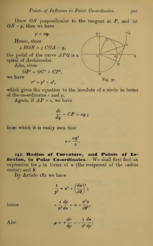
Points of Inflexion in Polar Co-ordinates. 301
Draw ON perpendicular to the tangent at P, and let
ON = p 9then we have
p = aq>.
Hence, since
LBON= l COA =<j>,
the pedal of the curve APQ is aspiral of Archimedes.
Also, since
we haveOP2 = OC2 + CP\
r2 = p2 + a2
,
Fig. 37.
which gives the equation to the involute of a circle in terms
of the co-ordinates r and p.
Again, if AP = s9we have
ds= CP = a<p;
from which it is easily seen that
« =
242. Radius of Curvature, and Points of In-flexion, in Polar Co-ordinates.—We shall first find anexpression for p in terms of u (the reciprocal of the radius
vector) and 0.
By Article 1 83- we have
hence
Al 80
I2-
2= u2 +
o2
fdu\*
1 dp
p*du
d 2uU+oW2
'
dr 1 du
dp u* dp
302 Radius of Curvature.
consequently ,(w+ g)» JL_ i +
'
wrffl
<**«
U + W(15)
i , rfw i drAgain, since u -, we nave -^ = - — ^,
rf2w 2 A^\ 2
i rfVand W =
?\dd)~?d02;
MDTp =
rfv—TrfAi'(l6)
This result can also be established in another manner, as
follows:
—
On reference to the figure of Art. 1 80, it is obvious that
eh = 6 + \p] where </> is the angle the tangent at P makes with
the prime vector OX.
dd> d\p d<f> ds dxpHence
5e= I+
S»'0T^dd = l+
Jd'>
" p d$ <&
dr d 2r i
Again, denotingjQ
and -^ by r and r, we have
tan \L « - : and hencer
*2 " '.2^ • . r - rr r* -rr
• • 1 +^ =i
-— '*also ^ = {r + r
'
d0 r2 + r
2 dv

Hence, we get p = -j
Intrinsic Equation of a Curve. 3°3
- rr + zr %
Or, replaciug f and r by their values,
'dr\*\i
rfV /drV
Again, since p = oo at a point of inflexion, we infer that
the points of intersection of the curve represented by the
equation
(Pr (dr\
with the original curve, determine in general its points of
inflexion.
In some cases the points of inflexion can be easier foundby aid of (15), which gives, when p = 00,
d 2u
Examples.
1. Find the radius of curvature at any point in the spiral of Archimedes,
(» + 0')*t - ad. Ans. a ^-.
2 + 9*
2. Find the radius of curvature of the logarithmic spiral r — a .
Ans. r(i + (loga)2)*.
3. Find the points of inflexion on the curve
ar = 29 - 1 1 cos id. Ans. cos 20 = —
.
11
4. Prove that the circle r - 10 intersects the curve
r = 11 — 2 cos $9
in its points of inflexion.
-. Prove that the curve
r - a + b cos n9
has no real points of inflexion unless a is > b and <(l + n2)b. When a lies be-tween these limits, prove that all the points of inflexion lie on a circle ; and showbow to determine the radius of the circle.

304 Radius of Curvature.
2\2 (a). Intrinsic Equation of a Curve.—In manycases the equation of a curve is most simply expressed in
terms of the length, s, of the curve, measured from a fixed
point on it, and the angle, 0, through which it is bent,
1. e. the angle of deviation of the tangent at any point fromthe tangent at the fixed point, taken as origin. These are
styled the intrinsic elements of the curve by Dr. Whewell,*to whom this method of discussing curves is due.
The relation between the length s and the deviation for
any curve is called its intrinsic equation.
If this relation be represented by the equation
then if p be the radius of curvature at any point, we have
,.-£-,-<,>.
Also, if sx denote the length of the evolute, from Art. 237
it is easily seen that the equation of the evolute is of the form
81 =//
(<?>) + const.
From this it follows that the series of successive evolutes
are in this case easily determined by successive differentiation.
The simplest case of an intrinsic equation is that of the
circle, in which case we have
s = a<j>.
Again, from Art. 241(a), the intrinsic equation of the
involute of a circle is reducible to the form
a<j>2
s = -21.
2
We shall meet with further examples of intrinsio equa-
tions subsequently.
243. Contact of Different Orders.—As already
stated, the tangent to a curve has a contact of the first order
with the curve at its point of contact, and the osculating
circle a contact of the second order. We now proceed to
distinguish more fully the different orders of contact between
two curves.
* Cambridge Philosophical Transactions , Vols. viu. and ix.

Contact of Different Orders. 305
Suppose the curves to be represented by the equations
y =/», and?/ = <j>(x),
and that <r, is the abscissa of a point common to both curves,
then we have
Again, substituting r x + A, instead of # in both equations,
and supposing y xand y2 the corresponding ordinates of the
two curves, we have
V, =/(*. + h) =/(*,) + hf(xx) + ^/>.) + &c.,
y2 - (#1 + A) = <j> (xi) f h(p\xi) + </>"(#i) + &c -
Subtracting, we get
*-*-*l/>0 -*'(*)} + 77; (TM ->.)} + &<>• (17)
Now, suppose y(a?i) 4>'(#i), or that the curves have a
common tangent at the point, then
1.2 1 . 2 . 3
In this case the curves have a contact of the first order
;
and when h is small, the difference between the ordinates is
a small quantity of the second order, and as y {- y2 does not
change sign with h9the curves do not cross each other at the
point.
If, in addition
then Vl - * - —— {/">,) - f>,) } + &c.1.2.3
In this case the difference between the ordinates is an in-
finitely small magnitude of the third order when h is takenan infinitely small magnitude of the first; the curves are
then said to have a contact of the second order, and approachinfinitely nearer to each other at the point of contact than in

306 Radius of Curvature.
the former case. Moreover, since y x- y2 ^anges its sign
with A, the curves cut each other at the point as well as touch.
If we have in addition /'"(#i) = 0"'(#i), the curves are
said to have a contact of the third order: and, in general, if
all the derived functions, up to the nth inclusive, be the samefor both curves when x = av the curves have a contact of the
nth order, and we have
hn+i
yi - y2 = {/(w+1)
(*0 - (n+1)(*0 ) + &o. (18)
n +
Also, if the contact be of an even order, n + i is odd, andconsequently h*+l changes its sign with A, and hence the curves
out eac other at their point of contact ; for whichever is the
lower at one side of the point becomes the upper at the
other side.
If the curves have a contact of an odd order, they do not
cut each other at their point of contact.
From the preceding discussion the following results are
immediately deduced :
—
(i). If two curves have a contact of the nth order, no curve
having with either of them a contact of a lower order can
fall between the curves near their point of contact.
(2). Two curves which have a contact of the n th order at
a point are infinitely closer to one another near that point
than two curves having a contact of an order lower than
the nth.
(3). If any number of curves have a contact of the second
order at a point, they have the same osoulating circle at the
point.
244. Application to Circle.—It can be easily verified
that the circle which has a contact of the second order with a
curve at a point is the same as the osoulating circle determined
by the former method.
For, let (X-a)2 + (F-|3) 2 = jR2
be the equation of a circle having contact of the second order
at the point (#, y) with a given curve ; then, by the preceding,7 72
the values of -7- and -7-^ must be the same for the circle anddx dx"
for the curve at the point in question.

Application to Circle. 307
Differentiating the equation of the circle twice, and sub-
stituting x and y for X and Y, we get
*-a + (y-0)£ = o, (19)
and «*&-fts? + (£)-* (*>)
1T ^ \dxj axlience y - p -75 , # - a =
1 + Dl
iP - s - a)' + (y - /32) = L W J
'rfy
(21)
t&7
This agrees with the expression for the radius of curvature
found in Art. 226.
The co-ordinates a, j3 of the centre of curvature can
be found by aid of equations (21) ; and the equation of the
e olute by the elimination of x and y between these equa-
tions and that of the curve.
In practice, the following equations aire often more useful :
thus, by differentiation with respect to x> we get from (19),
In like manner, from the equation
[y - 0) + (x - a) -r - O,
we obtain
<Px d ( dx\ , xa— = I + — [x— . (23)rfy
2 rfy\ dy
245. Centre of Curvature, and E volute ofEllipse.—As an illustration, we shall apply these equations to de-
x 2

308 Radius of Curvature.
terrnine the co-ordinates of the centre of curvature, and the
equation of the evolute of the ellipse
x2 y2
a2 b2
dy b% dx
dx a2 dy
-r-r ay u ax w
d I dy\ b2 d I dx\ d#2
dx\P dx) a? dy\dy) b2
'
„ cPy b2 (dy\% b
2 V x%
Hence ^ =-^-U)
='^~"V
b2( b
2x2
2 W2a2y2) a2
y
In like manner, we have
d 2x aK
xdy2
b2x2'
Substituting in (22) and (2$), we obtain for the co-ordinates
of the centre of curvature
P £. « = —~< (24)
Again, substituting the values of 2 and y given by these
Lations, in t
of the evolute
x ifequations, in the equation - + -= i,we get for the equation
(aa)l + (j3ft)I = {a2 - b
2)\.
246. It may be noticed that the osculating circle cttts the
curve in general, as well as touches it. This follows fromArticle 243, since the circle has a contact of the second order
at the point.
At the points of maximum and minimum curvature the

Osculating Curves, 309
osculating circle has a contact of the third order with the
curve ; for example, at any of the four vertices of an ellipse
the osculating circle has a contact of the third order, and does
not cut the curve at its point of contact (Art. 240)^
247. Osculating Curves.—When the equation of a
curve contains a number, u, of arbitrary coefficients, we can
in general determine their values so that the curve shall have
a contact of the (n - i)th order with a given curve at a given
point ; for the n arbitrary constants can be determined so
that the n quantities
dp (Py dT*yVy dx
y
dx2 ' ' ' (kTv
shall be the same at the point in the proposed as in the
given curve, and thus the curves will have a contact of the
(n - i)th order.
The curve thus determined, which has with a given curve
a contact of the highest possible order, is called an osculating
curve, as having a closer contact than any other curve of the
same species at the point.
For instance, as the equation of a circle contains but
three arbitrary constants, the osculating circle has a contact
of the second order, and cannot, in general, have contact of a
higher order ; similarly, the osculating parabola has a contact
of the third order ; and, since the general equation of a conic
contains five arbitrary constants, the general osculating conic
has a contact of the fourth order. In general, if the greatest
number of constants which determine a curve of a given
species be n, the osculating curve of that species has a contact
of the (n - 1)** order.
248. Geometrical Method.—The subject of contact
admits also of being considered in a geometrical point of view ;
thus two curves have a contact of the first order, when theyintersect in two consecutive points ; of the second, if they inter-
sect in three ; of the nth, if in n + 1 . For a simple investi-
gation of the subject in this point of view the student is
referred to Salmon's Conic Sections, Art. 239.
249. Curvature at a Double Point.—We now pro-
ceed to consider the method of finding the radii of curvatureof the two branches of a curve at a double point.

310 Radius of Curvature.
In this case the ordinary formula (8) becomes indetermi-
nate, since
du . du— = o, and — = oax dy
at a double point. The question admits, however, of beingtreated in a manner analogous to that already employed in
Art. 230 : we commence with the case of a node.
250. Radii of Curvature at a Node.—Suppose the
origin transferred to the node, and the tangents to the twobranches of the curve taken as co-ordinate axes, o> represent-
ing the angle between them.
By Art. 210, the equation of the curve is in this case of
the form
zhxy = of + fix2y + yxy2 + 8y* + uK + &o.
:
dividing by xy we obtain
X t/2
Ma2A = a- + j3# + 7y + S— + — + &C
y x xy
Now, let pi and p2 be the radii of curvature at the origin
for the branches of the curve which touch the axes of x and y,
respectively; then, by Art. 231, we have
x2y
2
2pi sin en = — , and 2p2 sin w = — , in the limit.
V *
Again, it can be readily seen, as in the note to Art. 230,
that the terms in — , &c, become evanescent along with xxy
x 9/
and y, and accordingly the limiting values of — and — cany x
be separately found, as in the Article referred to.
Hence we obtain
hP l
=•
9 P* §-- •• (
2 5)a sin id o sin w
Also, if a = o, we get p x= 00, and the corresponding
branch of the curve has a point of inflexion at the origin.
Similarly, if 8 = o, p2 = 00.

Radii of Curvature at a Cusp. 3 1
1
If a = o, and 8 = 0, the origin is a point of inflexion onboth branches. This appears also immediately from the
consideration that in this case uz contains u2 as a factor.
If the equation of a curve when the origin is at a nodecontain no terms of the third degree, the origin is a point of
inflexion on both branches. An example of this is seen in
the Lemniscate, Art. 210.
Examples.
1. Find the radii of curvature at the origin of the two branches ot the curve
ax* - 2bxy + cyz = xi + y4,
b bthe axes being rectangular. Am. - and -.
a e
2. Find the radii of curvature at the origin in the curve
a (y2 - x l
) = X*,
Transforming the equation to the internal and external bisectors of the angle
between the axes, it becomes
$axy y/z = {x-yf\
hence the radii of curvature are 2a y' 2 and - 2av 2 > respectively.
251. Radii of Curvature at a Cusp.—The preceding
method fails when applied to a cusp, because the angle wvanishes in that case. It is easy, however, to supply an in-
dependent investigation : for, if we take the tangent andnormal at the cusp for the axes of x and ?/, respectively, the
equation of the curve, by the method of Art. 210, may be
written in the form
y1 = ax3 + (3x
2y + yxy2 + $y* + u4 + &c. (26)
Now in this, as in every case, the curvature at the origin
depends on the form of the portion of the curve indefinitely
near to that point ; consequently, in investigating this formwe may neglect ?/V, ?/
3, &c, in comparison with y
2; and x4
x*y, &c., in comparison with x*.

3 1
2
Radius of Curvature.
Accordingly, the curvature at the origin is the same, in
general, as that of the cubic
y2 = ax* + fix
2y. (27)
Dividing by #2, we get
*- = ax + |3y.a2
Hence, in immediate proximity to the origin, be-X
comes very small, i. e. y is very small in comparison with x.
Accordingly, the form of the curve near the origin is repre-
sented by the equation
y2 = aa?.
From this we infer that the form of any algebraic curve
near a cusp is, in general, a semi-cubical parabola (see Ex. 2,
Art. 211).
Again, since
xk x
we have, by Art. 230,
\a
from which we see that p vanishes along with x, and accord-
ingly the radii of curvature are zero for both branches at the
origin.
This result can also be arrived at by differentiation, byaid of formula (
i)
.
252. Case where the Coefficient of x3 is wanting.—Next, suppose that the term containing x3 disappears, or
a = o, then the equation of the curve is of the form
// = fix?y + yxy2 + S;/3 + aV + &c.
;
and proceeding as before, the curvature at the origin is the
same as in the curve
y2 - ftx
2y + a'x\ (28)

Radii of Curvature at a Cusp. 313
The two branches of this curve are determined by the
equation
r-|^±YV^M7. (29)
The nature of the origin depends on the sign of j32 + 4a', and
the discussion involves three cases.
(1). If |32 + 4a 7 be positive, it is evident that the curve
extends at both sides of the origin, and that point is a doable
cusp (Art. 215(a)).
On dividing equation (28) by y2> and substituting 2p for
x2
—, we get 1 = 2j3/o + 4«V- (3°)
The roots of this quadratic determine the radii of curva-
ture of the two branches at the cusp.
These branches evidently lie at the same, or at opposite
sides of the axis of x, according as the radii of curvature
have the same or opposite signs : 1. e. according as a has a
negative or positive sign.
These results also appear immediately from the circum-
stance, that in this case the form of the curve very near the
origin becomes that of the two parabolas represented byequation (29).
(2). If fi2 + 4a be negative, y becomes imaginary, and the
origin is a conjugate point.
(3). If /32 + 4a' = o, the equation (30) becomes a perfect
square : we proceed to prove that in this case the origin is a
cusp of the second species.
To investigate the form of the curve near the origin, it is
necessary in this case to take into account the terms of the
fifth degree in x (y being regarded as of the second) : this gives
(y _ & x*y = yxtf + j3Vy + aV = x(yy2 + j3Vy + aV). (31)
It will be observed that the right-hand side changes its
sign with x ; accordingly the origin is a cusp. Also, the cuspis of the second species, for the two roots of the equation in yplainly have the same sign, viz., that of |3 ; and consequentlyboth branches of the curve at the origin lie at the same side
of the axis of x.
3 14 Radius of Curvature.
Moreover, as equation (30) has equal rooib in this case,
the radii of curvature of the tivo branches are equal, and thebranches have a contact of the second order.
We conclude that when the term involving x% in equation
(28) disappears, the origin is a double cusp, a cusp of the second
species, or a conjugate point, according as fi2 + 4a' > = or < o.
Moreover, if a = o, one root of the quadratic (30) is in-
finite, and the other is — . The origin in this case is a double2\5
cusp, and is also a point of inflexion on one branch. Such a
point is called a point of oscul-inflexion by Cramer.If j3 = o in addition to a = o, the origin is a cusp of the
first species, but having the radii of curvature infinite for bothbranches.
It is easy to see from other considerations that the radii
of curvature at a cusp of the first species are always either
zero or infinite.
For, since the two branches of the curve in this case
d 2
yturn their convexities in opposite directions, -
2must have
ax
opposite signs at both sides of the cusp, and consequently it
must change its sign at that point ; but this can happen only
in its passage through zero, or through infinity.
It should be observed that the preceding discussion applies
to the case of a curve referred to oblique axes of co-ordinates,
provided that we substitute 7 instead of p ; where y is half
the chord intercepted on the axis of y by the osculating circle
at the origin.
253. Recapitulation.—The conclusions arrived at in the
two preceding Articles may be briefly stated as follows :
—
( 1) . Whenever the equation of a curve can be transformed
into the shape y1 = aa? + terms of the third and higher degrees,
the origin is a cusp of the first species ; both radii of curva-
ture being zero at the point.
(2). When the coefficient of x3 vanishes,* the origin is
* In this case, if V\ be the equation of the tangent at the cusp, the equation
of the curve is of the form
t>l2 + V\V2 -t- vi + &c. = o.
This is also evident from geometrical considerations.

General Investigation of Cusps. 3 1
5
generally either a double cusp, a conjugate point, or a cusp
of the second species. In the latter case the two branches
of the curve have the same centre of curvature, and conse-
quently have a contact of the second order with each other.
(3). If the lowest term in x (independent of y) be of the
5th degree, the origin is a point of oscul-inflexion.
If, however, the coefficient of x2y also vanish, the origin
is not only a cusp of the first species, but also a point of
inflexion on both branches of the curve.
254. Oeneral Investigation of Cusps.—The pre-
ceding results admit of being established in a somewhat moregeneral manner as follows :
—
By the method already given, the equation which deter-
mines the form of an algebraic curve near to a cusp may bewritten in the following general shape :
y2 = iAxa
y + Bxb + Cx% (32)
where iAxais the lowest term in the coefficient of y, and
Bxb, Cx°* are the lowest terms independent of y.
By hypothesis, r/, b, c are positive integers, and a > 1, b> 2,
c > 3 ; now, solving for y, we obtain
y = Axa ± ^A2x2a + Bxh + Oaf,
which represents two parabolasf osculating the two branches
at the origin.
The discussion of the preceding form for y resolves itself
into three cases, according as za is > = or < b.
(1). Let 2a = b + h, then
b + h b
y = Ax*± xl yB + ASx* + Cxc~\
b
(a). If b be odd, x2 becomes imaginary for negative values
of x, and accordingly the origin is a cusp of the
first species in this case.
* This term is retained, as it is necessary in the case of a cusp of the second
species.
t The word parabola is here employed in its more extensive signification.
3 1
6
Radius of Curvature.
((5). If b be even, and B positive, y is real for all values
of x near the origin ; accordingly that point is a
double cusp.
(y). If b be even, and i? negative, the origin is a conjugate
point.
(2). If 2a = b, we have
y = A&±<xfi </{A2 + 5) + Oaf-*.
In this case,- the origin is either a double cusp, or a conju-
gate point, according as A2 + B is positive or negative.
Again, if A 2 + B = o, we have
y-s-^l + # 2 y/C).
(a). If - b be an odd number, the origin is a cusp of the
second species.
(j3). If c - b be even, the origin is a double cusp or a con-
jugate point according as C is positive or negative.
(3). 2a < b}or b = 2a + h.
Here y = Aafi ± x* ^/
A
2 + Bxh + Cxc~2a,
and the curve evidently extends at both sides of the origin,
which accordingly is a doable cusp.
This method of investigating curvature is capable of being
modified so as to apply to the case of multiple points of a
higher order ; the discussion, however, is neither sufficiently
elementary, nor sufficiently important, to be introduced here.
255. Points on £volute corresponding to €usns onCurve.—In connexion with evolutes and involutes, the pre-
ceding results lead to a few interesting conclusions.
(1). If a curve has a cusp of the first species, its evolute
in general passes through the cusp. However, if in addition
the cusp be a point of inflexion, the normal at it is an asymp-tote to the evolute.
(2). To a cusp of the second species corresponds in general
a point of inflexion on the evolute : in some cases the point
of inflexion lies altogether at infinity.
(3). To a double cusp corresponds a double tangent to the
evolute.

Equation of Osculating Conic. 3 1
7
256. Equation of the Osculating Conic.—As an
additional illustration of the principles involved in the pre-
ceding investigation, it is proposed to discuss the question of
the conic which osculates an algebraic curve at a given point-
Transferring the origin to the point, and taking the tangent
as axis of xy the equation of the curve may be written in the
form
ay = x* + axxy + a^y2 + b a? + b x x?y + b2xy
2 + fay*
+ e xi + c xxzy + &c. + d^ + &o. (33)
In considering the form of the curve near the origin, as a
first approximation we may, as in Art. 251, neglect xy, y\ &c,
in comparison with y ; and a?*, x\ &c, in comparison with x2
;
thus the equation reduces to the form
iv - **. (34)
Hence the form to which every curve of finite curvature
approximates in the limit is that of the common parabola, as
already seen in Art. 231.
To proceed to the next approximation, we retain terms of
the third order (remembering that when x is a very small
quantity of the first order, y is one of the second), and the
equation becomes
ay = a? + axxy + b x*.
On substituting ay instead of x2 in the term & #3, the pre-
ceding equation becomes
ay = x2 + (ax + b a) xy. (35)
This represents a conic having contact of the third order
with the proposed curve at the origin. When a x + b a = o, the
parabola ay = x2 has a contact of the third order at the origin,
and accordingly so also has the osculating circle.
In proceeding to the next and final approximation, we re-
tain terms of the fourth order, and we get
ay «= x2 + a xxy + a2y2 + b x* + b x x
2y + c x*. (36)

3 1
8
Radius of Curvature.
Moreover, from the preceding approximation we have
Kaxy = b x* + b x2
y (a x 4 ab ).
Henee, we get for the equation of the conio having a
contact of the olosest kind with the given curve
ay = x2 + («i + b a) my + \jh + a(6, - a x b ) + a2 (c - b2
)]y2. (37)
This conic, since it has the closest contact possible with
the given curve at the origin, is the osculating conic ("Art. 246)
for that point.
In like manner the parabola
ay = x2 + (a { + b a) xy + v'- y
2> (38)
4
since it has the closest contact possible for a parabola, is the
osculating parabola at the point.

Examples. 3 1
9
Examples.
1. Prove that the radius of curvature at the vertex of a parabola is equal to
its semi-latus rectum.
2. Find the length of the radius of curvature at the origin in the curve
yl » x3 + a (x2 f y
2) = a2
y. Ant. -,
3. Find the radius of curvature at the origin in the curve
a2y = bx2 v cx*y. Ans. 00.
4. Prove that the locus of the centre of a conic having contact of the third
order with a given curve at a common point is a right lino.
5. Prove that the locus of the centres of equilateral hyperbolas, which havecontact of the second order with a given curve at a fixed point, is a circle, whoseradius is half that of the circle of curvature at the point.
6. Prove geometrically that the centre of curvature at any point on an ellipse
is the pole of the tangent at the point, with respect to the confocal hyperbolawhich passes through that point.
7. The locus of the centres of ellipses whose axes have a given direction, andwhich have a contact of the second order with a given curve at a common point,
is an equilateral hyperbola passing through the point?
8. Prove that the locus of the focus of a parabola, which has a contact of
the second order with a given curve at a given point, is a circle.
9. Prove that the radius of curvature of the curve a171' 1 y = xm at the origin is
azero, -, or infinity, according as m is < = or > 2 : m being assumed to be greater
than unity.
10. Two plane closed curves have tho same evolute : what is the difference
between their perimeters ?
Am. 2wd$where d is the distance between the curves.
1 1. Find the radius of curvature at the origin in the curve
3y = 44; - 15*2 - 3s3 :
find also at what points the radius of curvature is infinite.
12. Apply the principles of investigating maxima and minima to find the
greatest and least distances of a point from a given curve ; and show that the
problem is solved by drawing the normals to the curve from the given point.
(a). Prove that the distance is a minimum, if the given point be nearer to
the curve than the corresponding centre of curvature, and a maximum if it be
further.

320 Examples.
(It). If tho given point bo on the evoluto, show that the solution arrived nt
is neither n maximum nor a minimum ; and hence show that the circle of curva-
ture cuts as well as touches tho curve ut its point of contact.
i \. Find an expression for the whole length of the cvolute of an ellipse.
Ans- * i~«no
14. Find the radii of curvature at the origin of tho two branches of the curve
5 ax* ax 1
if - axy2 -4 axy2 - o. Ans. a and -.
2 4
15. Prove that the evoluto of the hypocycloid
*! + //I = a\
is the hypocycloid(a I £)• + (a - j8)f = id.
16. Find the radius of curvature at any point on the curve
y + \/'x (1 - x) - sin-1 y/x.
17. If the angle between the radius vector and the normal to a curve has a
maximum or a minimum value, prove that y = r ; where 7 is the semi-chord of
Curvature which passes through the origin.
18. If the co-ordinates of a point on a curvo be given by the equations
x - c sin 20 (I + cos id), y - c cos 20 ( 1 - cos 2 0),
find the radius of curvaturo at the point. Ans. <\c cos 30
19. Show that the evoluto of the curve
r2 - a2 = mp2
has for its equationr2 - ( I - m) a2 = mp%
.
20. If a and £ be the co-ordinates of the point on the ovolute corresponding
to the point («, y) on a curve, prove that
dy da-r "Jk + « ©•dx dp
21. If p be the radius of curvature at any point on a curve, prove that the
radius of curvature at the corresponding point in the evolute is --; where o>
is tho angle tho radius of curvature makes with a fixed line.
22. In a curvo, prove that
1 d (dyy
p dxm

Examples. 321
23. Find the equation of the evolute of an ellipse by means of the eccentric
angle.
24. Prove that the determination of the equation of the evolute of the
curve y - kx* reduces to the elimination of x between the equations
it. - ->. k2^ _ . . in - 1,
1
x zln~l
, and fi = kxn -\
n - 1 n - 1 n — 1 kn(n - \)xn -%
25. In figure, Art. 239, if the tangent to the evolute at P meet the parabolain a point 77, prove that 1IN is perpendicular to the axis of the parabola.
26. If on the tangent at each point on a curve a constant length measuredfrom the point of contact be taken, prove that the normal to the locus of thepoints so found passes through the centre of curvature of the proposed curve.
27. In general, if through each point of a curve a line of given length bedrawn making a constant angle with the normal, the normal to the curve locusof the extremities of this line passes through the centre of curvature of the pro-posed. (Bertrand, Cal. Iftf., p. 573.)
^This and the preceding theorem can be immediately established from geome-
trical considerations.
28. If from the points of a curve perpendiculars be drawn to one of its tan-gents, and through the foot of each a line be drawn in a fixed direction, pro-portional to the length of the corresponding perpendicular ; the locus of theextremity of this line is a curve touching the proposed at their common point.
Find the ratio of the radii of curvature of the curves at this point.
29. Find an expression for the radius of curvature in the curve /> = —p being the perpendicular on the tangent.
30. Being given any curve and its osculating circle at a point, prove thatthe portion of a parallel to their common tangent intercepted between the twocurves is a small quantity of the second order, when the distances of the pointof contact from the two points of intersection are of the first order.
Prove that, under the same circumstances, the intercept on a line drawnparallel to the common normal is a small quantity of the third order.
31. In a curve referred to polar co-ordinates, if the origin be taken on thecurve, with the tangent at the origin as prime vector, prove that the radius of
Tcurvature at the origin is equal to one-half the value of in the limit.
32. Hence find the length of the radius of curvature at the origin in the• YlCL
curve r = a sin nQ. Ana. p —r
2
33. Find the co-ordinates of the centre of curvature of the catenary ; andshow that the radius of curvature is equal, but opposite, to the normal.
34. If p, p be the radii of curvature of a curve and of its pedal at corre-sponding points, show that
p(2r2 -pp) =r3.2nd. Civ. Ser. Exam., 1878.
Y
( 3" )
CHAPTER XVIII.
ON TRACING OF CURVES.
257. Tracing Algebraic Curves.—Before concluding the
discussion of curves, it seems desirable to give a brief state-
ment of the mode of tracing curves from their equations.
The usual method in the case of algebraic curves consists
in assigning a series of different values to one of the co-ordi-
nates, and calculating the corresponding series of values of
the other ; thus determining a definite number of points onthe curve. By drawing a curve or curves of continuous cur-
vature through these points, we are enabled to form a tolerably
accurate idea of the shape of the curve under discussion.
In curves of degrees beyond the second, the precedingprocess generally involves the solution of equations beyondthe second degree : in such cases we can determine the series
of points only approximately.
258. The following are the principal circumstances to beattended to :
—
(1). Observe whether from its equation the curve is sym-metrical with respect to either axis; or whether it can bemade so by a transformation of axes. (2). Find the points
in which the curve is met by the co-ordinate axes. (3). De-termine the positions of the asymptotes, if any, and at whichside of an asymptote the corresponding branches lie. (4). De-termine the double points, or multiple points of higher orders,
if any belong to the curve, and find the tangents at such
points by the method of Art. 212. (5). The existence of
ovals can be often found by determining for what values of
either co-ordinate the other becomes imaginary. (6). If the
curve has a multiple point, its tracing is usually simplified bytaking that point as origin, and transforming to polar co-or-
dinates : by assigning a series of values to we can usually
determine the corresponding values of r, &c. (7). The points

On Tracing of Curves. 323
where the y ordinate is a maximum or a minimum are founddv
from the equation -j- = o : by this means the limits of the(IX
curve can be often assigned. (8). Determine when possible
the points of inflexion on the curve.
259. To trace the Curve y2 = x2
(x - a) ; a beiog sup-
posed positive.
In this case the origin is
a conjugate point, and the
curve cuts the axis of x at a
distance OA = a. Again,when x is less than 0, y is .
imaginary, consequently noportion of the curve lies to
the left-hand side of A.The points of inflexion, /
and i', are easily determined
d 2
yfrom the equation — = o ; the
(XX
corresponding value of x is — ; accordingly AN =.
3 ...Again, if TI be the tangent at the point of inflexion i, it
a ANcan readily be seen that TA = - =
.
J9 3.
. This curve has been already considered in Art. 213, and
is a cubical parabola having a conjugate point.
260. Cubic with three Asymptotes.—We shall next
consider the curve*
Fig. 38.
y2x + ey = ax* + bx2 + ex + d, (0
where a is supposed positive.
The axis of y is an asymptote to the curve (Art. 200), and
the directions of the two other asymptotes are given by the
equation
y2 - ax2 = 0, or y = ± x */a.
* This investigation is principally taken from Newton's Enumeratio Li-
nearum Tertii Ordinis.
Y 2

324 On Tracing of Curves.
If the term bx2 be wanting, these lines are asymptotes ; if b
be not zero, we get for the equation of the asymptotes
y = x a/ a + =, y-f x */ a + —— = o.
2*/a 2\/a
On multiplying the equations of the three asymptotes
together, and subtracting the product from the equation of
the curve, we get
ey = [c ) x + a:4#
this is the equation of the right line which passes through the
three points in which the cubic meets its asymptotes. (Art.
2 °4-)
Again, if we multiply the proposed equation by x, andsolve for xy, we get
xye l e
2
=— ± lax* + bxz + ex2 + dx + - : (2)2 V 4
from which a series of points can be determined on the curve
corresponding to any assigned series of values for x.
It also follows that all chords drawn parallel to the axis
of y are bisected by the hyperbola xy + - = o : hence we infer
that the middle points of all chords drawn parallel to anasymptote of the cubic lie on a hyperbola.
The form of the curve depends on the roots of the bi-
quadratic under the radical sign. (1). Suppose these roots
to be all real, and denoted by a, j3, 7, 8, arranged in order of
increasing magnitude, and we have
xy =— ± <ya (x - a)(x - j3)(o? - y)(x - 8).
Now when x is < a, y is real ; when x > a and < /3, y is
imaginary ; when x > )3 and < 7, y is real ; when x > 7 and
< 8, y is imaginary ; when x > 8, y is real.

Asymptotes, 325
We infer that the curve consists of three branches, extendingto infinity, together
with an oval lying
between the values
/3 and y for x.
The accompany-ing figure* repre-
sents such a curve.
Again, if either
the two greatest
roots or the twoleast roots becomeequal, the corres-
ponding point be-
comes a node.
If the interme-
diate roots become FiS- 39-
equal, the oval shrinks into a conjugate point on the curve.
If three roots be equal, the corresponding point is a cusp,
If two of the roots be impossible and the other two un-
equal, the curve can have neither an oval nor a double point.
If the sign of a be negative, the curve has but one real
asymptote.
261. Asymptotes.—In the preceding figure the student
will observe that to each asymptote correspond two infinite
branches ; this is a general property of algebraic curves, of
which we have a familiar instance in the common hyperbola.
By the student who is acquainted with the elementary
principles of conical projection the preceding will be readily
apprehended ; for if we suppose any line drawn cutting a
closed oval curve in two points at which tangents are drawn,and if the figure be so projected that the intersecting line is
sent to infinity, then the tangents will be projected into
asymptotes, and the oval becomes a curve in two portions,
each having two infinite branches, a pair for each asymptote,
as in the hyperbola.
The figure is a tracing of the curve
yxy2 + io8y = (x - 5) (x - 11) (x - 12).

3^6 On Tracing of Curves.
It should also be observed that the points of contact at
infinity on the asymptote in the opposite directions along it
must be regarded as being one and the same point, since they
are the projection of the same point. That the points at
infinity in the two opposite directions on any line must beregarded as a single point is also evident from the considera-
tion that a right line is the limiting state of a circle of in-
finite radius.
The property admits also of an analytical proof; for if
the asymptote be taken as the axis of xythe equation of the
curve (Art. 204) is of the form
yfa + fa = o,02
or y- -f-,
where fa is at least one degree lower than fa in x and y.
Now, when x is infinitely great, the fraction — becomes in
general infinitely small, whether x be positive or negative
;
and consequently the axis is asymptotic to the curve in both
directions.
262. To trace the Curve
azy
2 = bxx + x5,
where a and b are both positive.
Here ya% = ± x2(x + 6)i
The curve is symmetrical with respect
to the axis of x, and has two infinite
branches ; the origin is a double cusp.
The shape of the curve is exhibited in the
figure annexed. Fig. 40.
If b were negative, we should have
ya* = ± x2(x - b)%.
Here y becomes imaginary for values of x less than b;
accordingly, the origin is a conjugate point in this case : the
curve has two infinite branches as in the former case
263. To trace the Curve
a?y2 = 2abx2
y + xb.

Form of Curve near a Double Point, 327
From the form of its equation we see that the origin is
a point of oscu/-inflexion (Art. 251).Solving for y y
we can easily
determine any number of points
on the curve we please. It hastwo infinitebranches at opposite
sides of the axis of %, and a loop
at the negative side of that axis,
as exhibited in the figure.
264. To trace the CurveFig. 41.
x* + x2
y2 + y* = x (ax
2 - by2
).
(1). Let a and b have the
same sign, then the origin is
a triple point, having for its
tangents the lines
x = o, x */a + y \/b - o,
and x^/a-y <s/b = o.
Moreover, since the curve
has no real asymptote, it is
a finite or closed curve with
three loops passing through the Fis* 4*-
origin ; and it is easily seen that its shape
is that represented in the accompanyingfigure.
(2). If a and b have opposite signs, the
lines represented by ax2 - by2 = o becomeimaginary. The curve in this case consists
of a single oval as in the figure.
This and the preceding figure were
traced for the case where b = 3a: if the
value of - be altered, the shape of the curve Fig. 43.
will alter at the same time. If a be greater than 6, the
curve (2) will lie inside the tangent at the point X.
265. Form of Curve near a Double Point.—When-ever the curve has a node or a cusp, by transforming the
origin to that point, the shape of the curve for the branches

328 On Tracing of Curves,
passing through the point admits of being investigated by the
method explained in Arts. 250, 251. It is unnecessary to
enter into detail on this subject here, as it has been already
discussed in the articles referred to.
266. In connexion with the tracing and the discussion of
curves there is an elementary general principle which maybe introduced here.
If the equation of a curve be of the form
LU - MM' - o,
where L, M, L\ Mr
are each functions of the co-ordinates x
and y, the curve evidently passes through all the points
of intersection of the curves represented by the equations
L = o and M = o ; similarly it passes through the intersec-
tions of L = o and M' = o ; and also those of M = o andI! = o ; and of 1! = o and M' = o. Moreover, if L and L'become identical, the points of intersection coincide in
pairs, and the equation of the curve becomes of the formL2 - MM' = o ; which represents a curve touching the curves
M = o, M' = o, at their points of intersection with the curve
L = o.
This principle admits of easy extension; but as the subject
belongs properly to the method of trilinear co-ordinates, it is
not considered necessary to enter more fully into it here.
267. On Tracing Curves given in Polar Co-ordi-nates.—The mode of procedure in this case does not differ
essentially from that for Cartesian co-ordinates. We have
already, in Arts. 206 and 207, considered the method of
finding the asymptotes and asymptotic circles in such cases.
It need scarcely be observed that the number and variety of
curves whose discussion more properly comes under the
method of polar co-ordinates are indefinite. We propose to
confine our attention to a few varieties of the class of curves
represented by the equation
rm = am cos mO.
268. On the Curves rm = am cos m9.—In this case,
since the equation is unaltered when is changed into - 0,
the curve is symmetrical with respect to the prime vector
:
again, when = o, we have r = a ; and as increases from zero

Curves of the Form rm = am cos mO. 329
to — , r diminishes from a to zero. When m is a positive in-2m
teger, it is easily seen that the curve consists of m similar loops.
There are many familiar curves included under this
equation. Thus, when m = 1, we have r = a cos 0, whichrepresents a circle : again, if m = - 1 , the equation gives
r cos = a, which represents a right line. Also, if m= 2, wehave r2 = a2
cos 2 0, a Lemniscate (Art. 210). If m = - 2, weget r2 cos 26 = a2
, an equilateral hyperbola.
If m = - we get r£ = ah cos -, whence r = - (1 + cos 0), a2 ° 2 2
v '
1 ft
cardioid (Ex. 4, p. 232) ; with m =, itis#4 cos - = «*, a
parabola (Ex. 1, p. 231) ; and so on. As already observed,
if we change m into - m we get a new curve, inverse of
the original. Also, the reciprocal polar is obtained by sub-771
stituting - instead of m.m + 1
The tangent and normal can be immediately drawn at
any point on a curve of this class by aid of the results arrivedat in Art. 190. The radius of curvature at any point hasbeen determined in Ex. 5, Art. 235. The method of findingthe equations of the successive pedals, both positive andnegative, has been also already explained.
A few examples in the case of fractional indices are hereadded.
Example 1.
rl = ah cos -.
3Here when = o, we have r = a,
and the curve cuts the prime vector
at a distance OA equal to a : again,
30^/3when = r =8
also when
e = ^ r = -, or OBo
Fig. 44-
The shape of the curve is given in the accompanyingfigure. This curve is the inverse of the caustic considered in
Example 18, p. 277.

330 On Tracing of Curves.
Ex. 2. Ex. 3. Ex. 4.
1 A C
rl = Af cos - 0. r* = at cos - 0. r* = a^ cos - 9.
4 5 3
In Ex. 2, as increases from zero to 120 , r diminishes
from a to zero : when 9 increases
from 120 to 240 , r increases fromzero to a : when increases from240 to 360 , r diminishes from a
to zero. By assigning negative
values to 9, the remaining part of
the curve is seen to be symmetrical (with that traced as above. Thesame result plainly follows by con-
tinuing the values for 9 from 360up to 720 . The form of the curve
is exhibited in the annexed figure. Fig. 45.
In Ex. 3, according as cos - 9 is positive or negative, we
get equal and opposite real values, or imaginary values, for r.
Hence it is easily seen that for values of 9 between ± - ir the
radius vector traces out two symmetrical portions of the
curve : again, between — tt and — w we get two other
Fig. 46. Fig. 47.
symmetrical portions. The shape is that given in the former
of the two accompanying figures.

The Limagon. 33i
The latter figure represents the curve in Ex. 4 ; it consists
of five symmetrical portions ranged round the origin.
The results above stated admit of generalization, and it
can be shown, without difficulty, that in general the curve-
p- p9rq = aq cos — consists of p similar portions arranged about
the origin ; and that the entire curve is included within a
circle of radius a when p is positive, but lies altogether
outside it when p is negative.
Many curves can be best traced by aid of some simple
geometrical property. We shall terminate the Chapter withone or two examples of such curves.
269. The Umaeon.—The inverse of a conic section
with respect to a focus is called a Limacon. From the polar
equation of a conic, its focus being origin, it is evident that
the equation of its inverse may be written in the form
r = a cos + b>
where a and b are constants.
It is easily seen that - is the eccentricity of the conic.
The curve can be readily traced by drawing from a fixed
point on a circle any number of chords, and taking off a
constant length on each of these lines, measured from the
circumference of the circle.
If a be less than b, the curve is the inverse of an ellipse,
and lies altogether outside the circle.
If a be greater than b, the
curve is the inverse of a hy-perbola, and its form can beeasily seen to be that exhibited
in the annexed figure, whereOB = a - b, and the point is anode on the curve.
If b = a, the curve becomesthe inverse of the parabola,and is called a cardioid. Theinner loop disappears in this
case, and the origin is a cuspon the curve. Fig. 48.

332 On Tracing of Curves.
When a= 2b, the Limacon is called the Triseotrix; acurve by aid of which any given angle can be readilytrisected.
270. The Conchoid of Nicomedes.—If through anyfixed point A a secant P
XAP be
drawn meeting a fixed right line LMin i2, and UP and PPX be taken
each of the same constant length
;
then the locus of P and P l is called
the conchoid.
This curve is easily traced fromthe foregoing geometrical property,
and it consists of two branches,
having the right line LM for a __
common asymptote. Moreover, if
the perpendicular distance AB of
A from the fixed line be less than
HP, the curve has a loop with a
node at A, as in the annexed figure.
It is easily seen that whenAB = EP, the point A is a cusp
on the curve ; and when AB is
greater than HP, A is a conjugate
point.
The form of the curve in the
latter case is represented by the dotted lines in the figure.
If AB = 0, RP = b, the polar equation of the curve is
(r ± b) cos 6 = a.
When transformed to rectangular co-ordinates, this
equation becomes
(;r + y2)(a-tf) 2 = b
2 x\
The method of drawing the normal, and finding thecentre of curvature, at any point, will be exhibited in thenext Chapter.
Examples. 333
Examples..
1. Trace the curve y = (x - 1) {x - 2) (x - 3), and find the position of its
point of inflexion.
2. Trace the curve yz - $axy +«3 = o, drawing its asymptote.
This curve is called the Folium of Descartes.
3. Tra the curve a2x -y(b2 4 x2), and find its points of inflexion, and
points of greatest and least distance from the axis of x.
4. If an asymptote to a curve meets it in a real finite point, show that the
corresponding branch of the curve must have a point of inflexion on it.
5. Find the position of the asymptotes and the form of the curve
xi — yi + 2axy2 = o.
6. Show that the curve r = a cos 20 consists of four loops, while the curve
r = a cos 3d consists of but three. Prove generally that the curve r = a cos nd
has n or 2w loops according as n is an odd or even integer.
7. Trace the curve
y2 (x - a){x - #) = c2 (x + a)(x + b).
8. Show that the eurve xiy2 + x* = a2 (x2 - y2) consists of two loops passing
through the origin, and find the form of the curve.
9. Trace the curve y(x + a) 4, = b2x{x + c)2, showing the positions of its
asymptotes and infinite branches.
10. Trace the curve whose polar equation is
r = a cos 6 + b cos 20,
and show that it consists of four loops passing through the origin.
n. Given the base and the rectangle under the sides of a triangle, find the
equation of the locus of the vertex (an oval of Cassini). Exhibit the different
forms of the curve obtained by varying the constants, and find in what case the
curve becomes a Lemniscate.
12. Trace the curve y2 = ax* -f ibx2 + t>cx + d
yand find its points ofgreatest
and least distance from the axis of x.
Show that two of these points become imaginary when the roots of the cubic
in x are all real.
13. Given the base and area of a triangle, prove that the equation of the
locus of the centre of a circle touching its three sides is of the form
x2y - a (x2 + y2)— b2 (y - a) = o.

334 Examples.
14. Prove that all curves of the third degree are reducible to one or other of
the forms
(1). xy2 + ey — ax3-f bx* + ex + d.
(2). xy = ax* + bx2 + ex + d.
(3). y2 = axz + bx2 + ex + d.
(4). y = as3 + bx2 + ex + d.
Newton, Enum. Linear. Ter. Ordinis.
15. Prove that all curves of the third degree can be obtained by projection
from the parabolas contained in class (3) in the preceding division. [Newton.]
For every cubic has at least one real point of inflexion : accordingly, if the
curve be projected so that the tangent at the point of inflexion is projected to
infinity, the harmonic polar (Art. 223) will bisect the system of parallel chords
passing through this point at infinity. Hence the projected curve is of the
class (3). [This proof is taken from Chasles, Histoire de la Geomeirie, note xx.]
a$216. Trace the curve r — --
, and show that it has a point of inflexionB" — 1
when $2 = 3 ; find also its asymptotes and asymptotic circle.
x17. Trace the curve y = «sin-, and show how to draw its tangent at any
a
point. (This is called the curve of sines.)
18. The base of a triangle is fixed in position ; find the equation of the locus
of its vertex, when the vertical angle is double one of the base angles.
Trace the locus in question, finding the position of its asymptote.
19. Show geometrically that the first pedal of a circle with respect to a
point on its circumference is a cardioid.
20. Show in like manner that the Liniacon is the first pedal of a circle with
respect to any point.
2 1
.
Trace the curve
«/4 + 2axy2 = axz + a?
4,
and find the equations of its asymptotes, and of the tangents at the origin.
Ind. Civ. Ser. Ex., 1876.

( 335
CHAPTER XIX,
ROULETTES.
271. Roulettes.—"When one curve rolls without sliding
upon another, any point invariably connected with the rolling
curve describes another curve, called a roulette.
The curve which rolls is called the generating curve, the
fixed curve on which it rolls is called the directing curve, or
the base, and the point which describes the roulette, the tracing
point. We shall commence with the simplest example of a
roulette : viz., the cycloid.
272. The Cycloid.—This curve is the path described by
a point on the circumference of a circle, which is supposed to
roll upon a fixed right line.
The cycloid is the most important of transcendental
curves, as well from the elegance of its properties as from its
numerous applications in Mechanics.
We shall proceed to investigate some of the most
elementary properties of the curve.
Let LPO be any position of the rolling circle, P the
generating point, the point of
contact of the circle with the fixed
line. Take the length AO equal
to the arc PO, then, from the
mode of generation of the curve,
A is the position of the generating
point when in contact with the
fixed line ; also, if AA be equal to the circumference of the
circle, A! will be the position of the point at the end of one
complete revolution of the circle. Bisect AA! in D, anddraw DB perpendicular to it and equal to the diameter of
the circle, then B is evidently the highest point in the
cycloid. Draw PN perpendicular to AA', and let PN = y,
AN = x, L PCO = 6, OC= a, and we get
* = AO-NO = a(0-f&nO), y = PN'- a(i -cos0). (1)
ANFig. 50.
336 Roulettes.
The position of any point on the cycloid is determined bythese equations when the angle is known, i. e. the anglethrough which the circle has rolled, starting from the position
for which the generating point is upon the directing line.
2 73' Cycloid referred to its Vertex.—It is often
convenient to refer the cycloid to its vertex as origin, and to
the tangent and normal at that point as axes of co-ordinates.
In the preceding figure let
x = BN', y = PN\ lPCL = V = tt-0;
then we have
x = BN' = a(0' + sin0'), y - PN' = a (i - cos 0'). (2)
274. Tangent and Normal to Cycloid.—It can be
easily seen that the line PO is normal at P to the cycloid
;
for the motion of each point on the circle at the instant is one
of rotation about the point 0, i. e. each point may be regarded
as describing at the instant an infinitely small circular* arc
whose centre is at : and hence PO is normal to the curve.
This result can also be established from the values of x
and y in (1) : for
dx , nv dy . n , x
—q - a{\ - cos 0), —Q= a sin : (3)
dy sin .$ , D T „.'. -f =
j. = cot - = cot PLO;
dx 1 - cos 2
and, accordingly, PL is the tangent, and PO the normal to
the curve at P.
Again, if we square and add the values of -^ and -^, we
obtain
^Y = a'{(1 - cos Oy + sin
26} = 4«
2 sin2 1
;
* This method of finding the normal to a cycloid is due to Descartes, and
evidently applies equally to all roulettes.

The Cycloid. 337
henceds
dO2a sm- = PO.
2(4)
275. Radius of Curvature and Evolute ofCycloid.—Let p denote the radius of curvature at the point P, and
lPOA =tf>= -;
then P =ds ds .9 ^^
2 — = 4« sin- = 2PO ;
2(5)
From this
Fig. 5'.
or the radius of curvature is double the normal,
value of p the evolute of the curve
can be easily determined. For,
produce PO until OP' = OP, then
P' is the centre of curvature be-
longing to the point P. Again,
produce LO until 00' = OL, anddescribe a circle through 0, P' andCf ; this circle evidently touches
AA\ and is equal to the generating
circle LPO.Also, the arc OP' = arc OP = ^0
;
.-. arc <7P' - 07*0 -P'0 = AD-AO=OD = B'O'.
Hence the locus of P' is the cycloid got by the rolling ofthis new circle along the line
B'O'-, and accordingly the evo-
lute of a cycloid is another
cycloid. It is evident that the
evolute of the cycloid ABA'is made up of the two semi-
cycloids, AB' and B'A\ as in
figure 51. Conversely, the
cycloid ABA' is an involute of
the cycloid AB'A'.The position of the centre of
curvature for a point P on a
cycloid can also be readily de-
termined geometrically, as fol-
lows :
—
Suppose O v a point on the
E'
Fig- 5*-
urcle infinitely near to 0, and take 002 = 00it LstPz

338 Roulettes.
be the centre of curvature required, and draw POi and P'02 ,
Now suppose the circle to roll until O x and 2 coincide, then
C02 becomes perpendicular to AD, and PO x and P'02 will
lie in directum (since P' is the point of intersection of twoconsecutive normals to the cycloid). Hence
L OCO, = L PO& = L OPO, + L OP'O,,
since each side of the equation represents the angle throughwhich the circle has turned.
But L OCO, = ilOP Ox. (Euclid, III. 20.)
Hence lOPO, = l OP'Or9
.-. POt = 1* Or,
and consequently in the limit we have
PO = P'O,as before.
We shall subsequently see that a similar method enables
js to determine the centre of curvature for a point in anyroulette.
276. JLengtli ofArc ofCycloid.—Since AP'B (Fig. 51)is the evolute of the cycloidAPP, it follows, from Art. 23 7, that
the arc APf
of the cycloid is equal in length to the line PF,or to twice Pf
; hence, as A is the highest point in the
cycloid AP'iy, it follows that the arc APf
measured from the
highest point of a cycloid is double the intercept P'O, madeon the tangent at the point by the tangent at the highest
point of the curve.
Hence, denoting the length of the arc AP' by s, we have
s = 4.a sin P'OD = \a sin (p. (6)
This gives the intrinsic equation of the cycloid (see Art.
242 (a)). Hence, also, the whole arc AB" is four times the
radius of the generating circle : and accordingly the entire
length ABA' of a cycloid is eight times the radius of its
generating circle.
Again, if the distance of P' from AA be represented byxj, we shall have
P'O2 = 00' xy = lay.
Hence s2 = $P'0* = 8ay. fj)

Epicycloids and Hypocycloids. 33Q
This relation is of importance in the applications of the
cycloid in Mechanics.
Again, since AO = arc OP' , if we represent AO by v, wehave*
V - 2tff (8)
277. Trochoids.— In general, if a circle roll on a
right line, any point in the.
plane of the circle carried round*
with it describes a curve. Suchcurves are usually styled tro-
choids. When the tracing
point is inside the circle, the
locus is called a prolate tro-
choid ; when outside, an oblate,
the accompanying figure.
Their equations are easily determined; for, let x, y be
the co-ordinates of a tracing point P, referred to the axes
AD, and AI (A being the position for which the movingradius CP is perpendicular to the fixed line).
Then, if CO = a, CP = d, L OOP = 9, we have
x = AN=AO- ON=aO-dsmO,\
y = PN = a - d cos 0. )
278. Epicycloidsf and Hypocycloids.—The investi-
ng. 53.
Their forms are exhibited in
* This is called, by Professor Casey, the tangential equation of the cycloid,
and by aid of it he has arrived at some remarkable properties of the curve (" Ona New Form of Tangential Equation," Philosophical Transactions, 1877). "Ingeneral, if a variable line, in any of its positions, make an intercept v on the axis
of or, and an angle<f>with it; then the equation of the line is
ar + 2/cot</> — v = o ;
and v,<J>,
the quantities which determine the position of the line may be called
its co-ordinates. From this it follows that any relation between v and <ptsuch
as
will be the tangential equation of a curve, which is the envelope of the line."For applications, the reader is referred to Professor Casey's Memoir. See also
Dub. Exam. Papers, Graves, Lloyd Exhibition, 1847.
f I have in this edition adopted the correct definition of these curves as
given by Mr. Proctor in his Geometry of Cycloids. I have thus avoided theanomaly existing in the ordinary definition, according to which every epicycloid
Z 2

340 Roulettes.
gation of the properties of the cycloid naturally gave rise to
the discussion of the more general case of a circle rolling on a
fixed circle. In this case the curve generated by any point
on the circumference of the rolling circle is called an epicycloid,
or a hypocycloid, according as the rolling circle touches the outside,
or the inside of the circumference of the fixed circle. We shall
commence with the former case.
Let P be the position of the generating point at any in-
stant, A its position whenon the fixed circle ; then
the arc OA = arc OP.Again, let Cand C be
the centres of the circles,
a and b their radii,
lACO = Q,L OC'P=&;then, since arc OA = arc
OP, we have ad = b9.
Now, suppose C taken
as the origin of rectangu-
lar co-ordinates, and CAas the axis of x ; draw PNand C'L perpendicular, FiS- i4
and P31 parallel, to CA, and we have
x=CN=CL-NL = (a + b) cos 6 - b cos (0 + 0').
y = PN=C'L-C'M= (a + b)smO-b sin (0 + 0');
aor, substituting - for 0',
x = (a + b) cos - b cos —j- 0.
. a + 6y = {a + b) sin - b sin —j— 0.
> IOI
is a hypocycloid, but only some hypocycloids are epicycloids. While according
to the correct definition no epicycloid is a hypocycloid, though each can be gene-
rated in two ways, as will be proved in Art. 280.

Epicycloids and Hypocycloids. 341
When the radius of the rolling circle is a submultiple of
that of the fixed circle, the tracing point, after the circle
has rolled once round the circumference of the fixed circle,
evidently returns to the same position, and will trace the
same curve in the next revolution. More generally, if the
radii of the circles have a commensurable ratio, the tracing
point, after a certain number of revolutions, will return to its
original position : but if the ratio be incommensurable, the
point will never return to the same position, but will describe
an infinite series of distinct arcs. As, however, the suc-
cessive portions of the curve are in every respect equal to
each other, the path described by the tracing point, fromthe position in which it leaves the fixed circle until it returns
to it again, is often taken instead of the complete epicycloid,
and the middle point of ihis path is called the vertex of the
curve.
In the case of the hypocycloid, the generating circle rolls
on the interior of the fixed circle, and it can be easily seen
that the expressions for x and y are derived from those in (10)
by changing the sign of b ; hence we have
x = (a - b) cos + b cos —j— 0,
a-b i
(I °y = (a - b) sin - b sin —— 0.
The properties of these curves are best investigated byaid of the simultaneous equations contained in formulas (10)
and (11).
It should be observed that the point A, in Fig. 54, is a
cusp on the epicycloid ; and, generally, every point in whichthe tracing point P meets the fixed circle is a cusp on the
roulette. From this it follows that if the radius of the rolling
circle be the nih part of that of the fixed, the corresponding epi-
or hypo-cycloid has n cusps : such curves are, accordingly,
designated by the number of their cusps : such as the three-
cusped, four-cusped, &c. epi- or hypo-cycloids.
Again, as in the case of the cycloid, it is evident fromDescartes' principle that the instantaneous path of the point Pis an elementary portion of a circle having as centre ; ac-
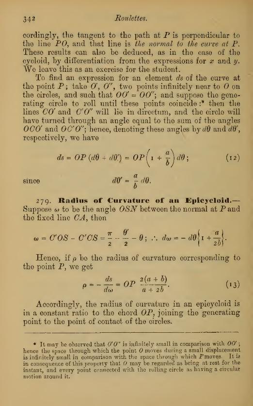
34 2 Roulettes.
cordingly, the tangent to the path at P is perpendicular to
the line PO, and that line is the normal to the curve at P.These results can also be deduced, as in the case of the
cycloid, by differentiation from the expressions for x and y.
We leave this as an exercise for the student.
To find an expression for an element ds of the curve at
the point P; take 0', 0", two points infinitely near to onthe circles, and such that 00' = 00"; and suppose the gene-
rating circle to roll until these points coincide :* then the
lines CO' and CO" will lie in directum, and the circle will
have turned through an angle equal to the sum of the angles
OCO' and OCO"; hence, denoting these angles by dd and dO',
respectively, we have
ds = OP (dO + dff) = Op(i + ~) dO; (12)
since dff = r dO.
279. Radius of Curvature of an Epicycloid.—Suppose (o to be the angle OSN between the normal at P andthe fixed line CA, then
w = COS- C'CS = ----0; .\ tfo^-^ji+^ri22 { 2b)
Hence, if p be the radius of curvature corresponding to
the point P, we get
,= * p 2ii±|). (I3)rda) a + 2b
Accordingly, the radius of curvature in an epicycloid is
in a constant ratio to the chord OP, joining the generating
point to the point of contact of the circles.
* It may be observed that O'O" is infinitely small in comparison with 00'\
hence the space through which the point moves during a small displacement
is infinitely small in comparison with the space through which Pmoves. It is
in consequence of this property that may be regarded as being at rest for the
instant, and every point connected with the rolling circle as having a circular
motion around it.

Double Generation of Epicycloids and Hypocycloids. 343
Fig. 55s
280. Double Generation of Epicycloids and Hypo-cycloids.—In an Epicycloid, it can be easily shown that
the curve can be generated in a second manner. For,suppose the rolling circle in-
closes the fixed circle, and join
P, any position of the tracing
point, to 0, the correspond-
ing point of contact of the twocircles; draw the diameter OED,and join O'E and PD ; connect
C, the centre of the fixed circle,
to 0', and produce CO' to meetDP produced in D', and describe
a circle round the triangle (/PD';this circle plainly touches the
fixed circle ; also the segmentsstanding on OP, O'P, and OC are obviously similar ; hence,
since OP = 00' + OP, we have
arc OP = arc 00' + arc O'P.
If the arc 00'A be taken equal to the arc OP, we havearc OfA = aro O'P; accordingly, the pointP describes the samecurve, whether we regard it as on the circumference of the
circle OPD rolling on the circle OO'E, or on the circumference
of O'PD' rolling on the same circle;provided the circles each
start from the position in which the generating point coincides
with the point A. Moreover, it is evident that the radius oj
the latter circle is the difference
between the radii of the other two.
Next, for the Hypocycloid,suppose the circle OPD to roll
inside the circumference of O'E,
and let be the centre of the
fixed circle;join OP, and pro-
duce it to meet the circum-
ference of the fixed circle in Of;
draw O'E and PD, join CO',
intersecting PD in D', and de-
scribe a circle round the triangle
PD'O\ It is evident, as be-
fore, that this circle touches the Fig. 5^

344 Roulettes.
larger circle, and that its radius is equal to the difference be-
tween the radii of the two given circles. Also, for the samereason as in the former case, we have
arc Off = arc OP + arc O'P.
If the arc OA be taken equal to OP, we get are O'P= arc O'A ; consequently, the point P will describe the samehypocycloid on whichever circle we suppose it to be situated,
provided the circles each set out from the position for which
P coincides with A.The particular case, when the radius of the rolling circle is
half that of the fixed circle, may be noticed. In this case the
point D coincides with (7, and P becomes the middle point of
00\ and A that of the arc Off. From this it follows im-
mediately that the hypocycloid described by P becomes the
diameter OA of the fixed circle. This result will be proved
otherwise in Art. 285.
The important results of this Article were given by Euler
(Acta.Petrop.y 1 78 1). By aid of them all epicycloids can be
generated by the rolling of a circle outside another circle
;
and all hypocycloids by the rolling of a circle whose radius
is less than half that of the fixed circle.
281. Evolute of an Epicycloid.—The evolute of an
epicycloid can be easily
seen to be a similar epi-
cycloid.
For, let P be the trac-
ing point in any position,
A its positionwhen on the
fixed circle;join P to 0,
the point of contact of the
circles, and produce PO
until PP= OP^,then P is the centre of
curvature by ( 1 3) ; hence
OF = OP -^—va + 20 Fig. 57.
Next, draw P'ff perpendicular to P'O; circumscribe the

Evolute of Epicycloid. 345
triangle OFCf by a circle ; and describe a circle with as
centre, and CO' as radius : it evidently touches the circle OP' (J.
Then 00' : OE = OP' : OP = a: a + 2b = CO : CE;
/. CO-OC:CE-OE = CO:CE}
or C(/:CO= CO : CE;
that is, the lines CE, CO, and CO' are in geometrical pro-
portion.
Again, join C to J?', the vertex of the epicycloid ; let CBmeet the inner circle in D, and we have
arc 0'D:arcOJ5 = CO' : C0= CO : CE = 00 .EO
= arc P'O' : arc OQ.
But arc OB = arc OQ ; .\ arc OB = arc P/
(/.
Accordingly, the path described by P' is that generated by a
point on the circumference of the circle OP'O' rolling on the
inner circle, and starting when P' is in contact at B. Hencethe evolute of the original epicycloid is another epicycloid.
The form of the evolute is exhibited in the figure.
Again, since CO : OE = CO' : O'O, the ratio of the radii
of the fixed and generating circles is the same for both epicy-
cloids, and consequently the evolute is a similar epicycloid.
Also, from the theory of evolutes (Art. 237), the line
PP' is equal in length to the arc FA of the interior epicy-
cloid ; or the length of P'A, the arc measured from the
vertex A of the curve, is equal to
*J^or, i0F c°:,2oP cc
co ca
Hence, the length* of any portion of the curve measuredfromits vertex is to the corresponding chord of the generating circle as
tivice the sum of the radii of the circles to the radius of the fixed
circle.
* The length of the arc of an epicycloid, as also the investigation of its
evolute, were given by Newton (Principia, Lib. 1., Props. 49, 50).

34^ Roulettes.
With reference to the outer epicycloid in Fig. 57, this
gives
arcPP^PP.-^. (14)
The corresponding results for the hypocycloid can befound by changing the sign of the radius b of the rolling
circle in the preceding formulae.
The investigation of the properties of these curves is of
importance in connexion with the proper form of toothed
wheels in machinery.282. Pedal of Epicycloid.-
with respect to the centre of the
fixed circle, admits of a very
simple expression. For let P be
the generating point, and, as be-
fore, take arc OA = arc OP, andmake AB = 90 . Join CA, CB>CP, and draw CN perpendicular
to DP. Let l PDO = 0, L BON= w,LACO = e, CN = p.
Then since AO = PO, we have
The equation of the pedal,
a9 = 2b(p = ^*.a
Again, w = go° -ACN= +
2 V-f 1 +
hence
Fig. 5*.
=rroj
a + 2b(15)
Also CN= CD sin 0;
,\ p = {a + 2b) sineta)
a + 2b9 (16)
which is the equation of the required pedal.
283. Equation of Epicycloid in terms of r and p.—Again, draw OL parallel to DiY, and let CP = r, and we have
r2 -p2 = PN2 - OL2 = OC 2 - CL2 = a2 -
a + 2bf\

Epitrochoids and Hypotrochoids. 347
hence r2 = a2 + -^—-~p2
. (17)(a + 2b) 2 x "
Also, from (16) it is plain that the equation of DN, the tan-
gent to the epicycloid (referred to GB and CA as axes of x
and y respectively), is
#cos 10 + y sin w = (a + 2 J) sin 7. (18)
The corresponding formulae for the hypocycloid are
obtained by changing the sign of b in the preceding equa-
tions.
Again, it is plain that the envelope of the right line re-
presented by equation (18) is an epicycloid. And, in general,
the envelope of the right line
x cos to + y sin w = k sin mw,
regarding w as an arbitrary parameter, is an epicycloid, or a
hypocycloid, according, as m is less or greater than unity. Forexamples of this method of determining the equations of epi-
and hypo-cycloids the student is referred to Salmon's Higher
Plane Curves, Art. 310.
284. Epitrochoids and Hypotrochoids.—In general,
\vhen one circle rolls on another, every point connected with
the rolling circle describes a distinct curve. These curves are
called epitrochoids or hypotrochoids, according as the rolling
circle touches the exterior or the interior of the fixed circle.
If d be the constant distance of the generating point fromthe centre of the rolling circle, there is no difficulty in
proving, as in Art. 278, that we have in the epitrochoid the
equations
x - {a + b) cos - d cos —— 0,
a + b> <*9)
y = (a + b) sin - d sin —7— 0.

348 Roulettes,
In the case of the hypotrochoid, changing the signs of hand d, we obtain
oc = {a - b) cos + d cos —— 0,
y = (a - 5) sin - tf sin ^— 0.[
(20)
In the particular case in which a = 2/;, i.e. when a circle
rolls inside another of double its diameter, equations (20)become
x = (b + d) cos 6, y = (b - d) sin 6
;
and accordingly the equation of the roulette is
x2if
(bTdf+
(b - d)2= l
;
which represents an ellipse whose semi-axes are the sum andthe difference of b and d.
This result can also be established geometrically in thofollowing manner :
—
285. Circle rolling inside another of double itsDiameter.—Join d and to anypoint L on the circumference of the
rolling circle, and let C{L meet the
fixed circumference in A ; then since
L OCL = 2OCA, and OC, = 2 00, wehave arc OA = arc OL ; and, accord-
ingly, as the inner circle rolls on the
outer the point L moves along CVA.In like manner any other point onthe circumference of the rolling circle
describes, during the motion, a dia-
meter of the fixed circle.
Again, any point P, invariably connected with the rolling
circle, describes an ellipse. For, if L and M be the points in
which CP cuts the rolling circle, by what has been just
shown, these points move along two fixed right lines C\Aand CiB, at right angles to each other. Accordingly, by a

Epitrochoids and Hypotrochoids. 349
well-known property of the ellipse, any other point in the
line LM describes an ellipse.
The case in which the outer circle rolls on the inner is
also worthy of separate consideration.
286. Circle rolling on another inside it and ofhalf its Diameter.—In this case, any diameter of the rolling
circle always passes through a fixed point, which lies on the
circumference of the inner circle.
For, let CiL and CJL be any two positions of the movingdiameter, Cx and C2 being the corresponding positions of the
centre of the rolling circle : and 2 the corresponding posi-
tions of the point of contact of the circles. Now, if the outer
circle roll from the former to the latter position, the right
lines Ci02 and C02 will coincide in
direction, and accordingly the outer
circle will have turned through the
angle C2 2Cl ; consequently, the mov-ing diameter will have turnedthrough the same angle ; and hence
L Cjj& = L C2 2 Ci ; therefore the
point L lies on the fixed circle, andthe diameter always passes throughthe same point on this circle.
Again, any right line connected
with the rolling circle will ahcays touch
a fixed circle.
For, let DE be the moving line in any position, and drawthe parallel diameter AB\ let fall CJ? andLM perpendicular
to DE. Then, by the preceding, AB always passes through
a fixed point L ; also LM= dF= constant ; hence DE always
touches a circle having its centre at L.Again, to find the roulette described by any carried point
Pi. The right line P1C1, as has been shown, always passes
through a fixed point L ; consequently, since dPi is a con-
stant length, the locus of Pi is a Limagon (Art. 269). In like
manner, any other point invariably connected with the outer
circle describes a Limacon ; unless the point be situated onthe circumference of the rolling circle, in which case the
locus becomes a cardioid.
Fig. 60.

350 Examples—Roulettes.
i. When the radii of the fixed and the rolling circles become equal, provegeometrically that the epicycloid becomes a cardioid, and the epitrochoid a
Limacon (Art. 269).
2. Prove that the equation of the reciprocal polar of an epicycloid, withrespect to the fixed circle, is of the form
r sin ma) = const.
3. Prove that the radius of curvature of an epicycloid varies as the perpen-
dicular on the tangent from the centre of the fixed circle.
4. If a = 4#, prove that the equation of the hypocycloid becomes
5. Find the equation, in terms of r and p, of the three-cusped hypocycloid;
i. e. when a = 3 3. Ans. r1 = a2 — %p2.
6. Find the equation of the pedal in the same curve.
Ans. p — b sin 3a.
7. In the case of a curve rolling on another which is equal to it in everyrespect, corresponding points being in contact, prove that the determination of
the roulette of any point P is immediately reduced to finding the pedal of the
rolling curve with respect to the point P.
8. Hence, if the curves be equal parabolas, show that the path of the focus
is a right line, and that of the vertex a cissoid.
9. In like manner, if the curves be equal ellipses, show that the path of the
focus is a circle, and that of any point is a bicircular quartic.
10. In Art. 285, prove that the locus of the foci of the ellipses described bythe different points on any right line is an equilateral hyperbola.
11. A is a fixed point on the circumference of a circle ; the points L and Mare taken such that arc AL = m arc AM, where m is a constant
;prove that the
envelope of LM is an epicycloid or a hypocycloid, according as the arcs AL andAM are measured in the same or opposite directions from the point A.
12. Prove that LM, in the case of an epicycloid, is divided internally in the
ratio m : 1, at its point of contact with the envelope ; and, in the hypocycloid,
externally in the same ratio.
13. Show also that the given circle is circumscribed to, or inscribed in, the
envelope, according as it is an epicycloid or hypocycloid.
14. Prove, from equation (14), that the intrinsic equation of an epicycloid is
±b (a + b) . ad>s = — sin
a + ib*
where s is measured from the vertex of the curve.
15. Hence the equation s = I sin ncp represents an epicycloid or a hypo-cycloid, according as n is less or greater than unity.

Centre of Curvature of an Epitrochoid or Hypotrochoid. 351
16. In an epitrochoid, if the distance, d, of the moving point from the centre
of the rolling circle be equal to the distance between the centres of the circles,
prove that the polar equation of the locus becomes
adr = 2 (a + b) cos 7.v ' a + 2b
17. Hence show that the curve
r = a sin mO
is an epitrochoid when m < 1, and a hypotrochoid when m > 1.
This class of curves was elaborately treated of by the Abbe Grandi in the
Philosophical Transactions for 1723. He gave them the name of " RhodoneaVfrom a fancied resemblance to the petals of roses. See also Gregory's Exampleson the Differential and Integral Calculus, p. 183.
For illustrations of the beauty and variety of form of these curves, as well as
of epitrochoids and hypotrochoids in general, the student is referred to the admi-rable figures in Mr. Proctor's Geometry of Cycloids.
287. CentreHypotrochoid.
-
of Curvature of an Epitrochoid or-The position of the centre of curvature for
any point of an epitrochoid can be easily
found from geometrical considerations. For,
let Ci and C2 be the centres of the rolling
and the fixed circles, P2 the centre of cur-
vature of the roulette described by P, ; and,
as before, let 0, and 2 be two points on the
circles, infinitely near to 0, such that OOi= 002 . Now, suppose the circle to roll until
0i and 2 coincide; then the lines C x Oi
and C2 2 will lie in directum, as also the
lines Pid and P2 % (since P2 is the point Fig. 61.
of intersection of two consecutive normals to
the roulette).
Hence L OC.O, + L OC2 2 = L OP.O, + L OP2 2,
since each of these sums represents the angle through whichthe circle has turned.
Again, let L COP, = 0, 00, - 002 = ds;
then L 00,0,ds --in ^
~~0C2
'OC L 0C2 0*
L0Pi0i_d*«*±
9LOP2 2
=d-^:

352 Roulettes.
consequently we have
i i
oc, ' oc2
= ecs^(0pi
+I
OP:
Or, if OP, = ru 0P2 = i%i i
~ + Ia o= COS d) (
— +ftJ
)•
(21)
From this, equation r2 , and consequently the radius of curva-ture of the roulette, can be obtained for any position of thegenerating point Pi.
If we suppose Pi to be on the circumference of the rolling
circle, we get cos <j> =*
; whence it follows that2 C/Oi
OP, = —^ OPr,a + 20
ivhich agrees with the result arrived at in Art. 279.2 88. Centre of Curvature of any Roulette.—The
preceding formula can be readily extended to any roulette : for
if d and 2 be respectively the centres of curvature of the
rolling andfixed carves, corresponding to the point of contact 0,we may regard 00\ and 002 as elementary arcs of the circles
of curvature, and the preceding demonstration will still
hold.
Hence, denoting the radii of curvature Od and 002 bypi and p2y we shall have
— + _ = COS d>( - 4- -J. (22)
Pi /o 2r\n r2J
It can be easily seen, without drawing a separate figure,
that we must change the sign of p 2 in this formula when the
centres of curvature lie at the same side of 0.
It may be noted that P x is the centre of curvature of the
roulette described by the point P2 , if the lower curve be sup-
posed to roll on the upper regarded as fixed.
289. Geometrical Construction* for the Centre of
* This beautiful construction, and also the formula (22) on which it is based,
were given by M. Savary, in his Lemons des Machines a V Ecole Folytechnique.
See also Leroy's Geometrie Descriptive, Quatrieme Edition, p. 347.

Construction for Centre of Curvature. 353
Curvature of a Roulette.—The formula (22) leads toa simple and elegant construction for the centre of curva-ture P2 .
We commence with the case when the base is a rightline, as represented in the accom-panying figure.
Join Pi to Cu the centre of curva-
ture of the rolling curve, and drawON perpendicular to 0PU meetingP,C, in N\ through N draw NM
4
parallel to OCi, and the point P2 in
which it meets OPi is the centre of
curvature required.
For, equation (22) becomes in
this caseFig. 62.
ocr cos<t>OP, 0P2)
\
whence we get
PiP2 _OP, . OP2 OC, sin d ON NCL sin &N0
P^NP,'
' OP, NCX
;
NP\NCl TOP l
and, accordingly, the line NP2 is parallel to 0CX . Q. E. D.The construction in the general case is as follows :
—
Determine the point N as in the former
jase, and join it to ft, the centre of curva-
ture of the fixed curve, then the point of
intersection of NC2 and P x is the required
centre of curvature. •
This is readily established ; for, from
the equation
we get0CX . OC,
CiCt OP,
0C2 P,P,
OPi . OP,
OC 1 cos<t>
~OP~'2 A
Fig. 63.

354
But, as before,
OCi cos <j>
hence
Roulettes.
CxN.OP x 0CX cos NCX
NPX OPx NP X
'
CXC2 0P2 NC^OC2 P xP2
~~NPX
Consequently, by the well-known property of a transversal
cutting the sides of a triangle, the points C2 , P2 , and N are
in directum.
The modification in the construction when the rolling
curve is a right line can be readily supplied by the student.
290. Circle of Inflexions.—The following geometrical
construction is in many cases more Cj
useful than the preceding.
On the line OC\ take OD x such
that
1 1
ODx 00, 002
and on OD xas diameter describe a
circle. Let E xbe its point of inter-
section with OPi, then we have
cos <j>=OEx
02V
smd formula (22) becomes
1 1
+OP x
TOP2
" 01) x cos"" OEx
m *23 '
Hence, if the tracing point P x lie on the circle* OExD x ,
* This theorem is due to La Hire, who showed that the element of the
roulette traced by any point is convex or concave with respect to the point of
contact, 0, according as the tracing point is inside or outside this circle. (See

Envelope of a Carried Curve. 355
the corresponding value of OP2 is infinite, and consequently
Pi is a point of inflexion on the roulette.
In consequence of this property, the circle in question is
called the circle of inflexions^ as each point on it is a point of
inflexion on the roulette which it describes.
Again, it can be shown that the lines PiP2 , PiO and P xE x
are in continued proportion ; as also C\C2, CiO, and CiD x .
For, from (23) we have
PiP2 1
OP, . OP2 OE{
Hence P,P2 :P,0= OP2 : OEx \
.: P^iPtO^PtPt-OPt-.PLO-OE^P.OiP^. (24)
In the same manner it can be shown that
C,C2 : 0,0 = C,0 : CXDX . (25)
In the particular case where the base is a right line, the
circle of inflexions becomes the circle described on the radius
of curvature of the rolling curve as diameter.
Again, if we take OD2 = ODiy we shall have, by describing
a circle on OD2 as diameter,
\j%\j\ *. L/ 2 (J = \s2 \J l \j 2D2 \
and also P2PX : P2 = P2 : P2E2. (26)
The importance of these results will be shown further on.
291. Envelope of a Carried Curve.—We shall next
consider the envelope of a curve invariably connected with the
rolling curve, and carried with it in its motion.
Since the moving curve touches its envelope in each of its
Memoires de VAcade'mie des Sciences, 1706.) It is strange that this remarkableresult remained almost unnoticed until recent years, when it was found to
contain a key to the theory of curvature for roulettes, as well as for the
envelopes of any carried curves. How little it is even as yet appreciated in
this country will be apparent to any one who studies the most recent produc-tions on roulettes, even by distinguished British Mathematicians,
2 A Z

35 6 Roulettes.
positions, the path of its point of contact at any instant mustbe tangential to the envelope; hence the normal at their
common point must pass through 0, the point of contact of
the fixed and rolling curves.
In the particular case in which the carried curve is aright line, its point of contact withits envelope is found by dropping a
perpendicular on it from the point of
contact 0.
For example, suppose a circle to
roll on any curve : to find the envelope*
of any diameter PQ :
—
From draw ON perpendicular
to PQ, then N, by the preceding, isFi 6
a point on the envelope.
On OC describe a semicircle ; it will pass through N,and, as in Art. 286, the arc ON = arc OP = OA, if A be
the point in which P was originally in contact with the
fixed curve. Consequently, the envelope in question is the
roulette traced by a point on the circumference of a circle
of half the radius of the rolling circle, having the fixed curve
A for its base.
For instance, if a circle roll on a right line, the envelope of
any diameter is a cycloid, the radius of whose generating circle
is half that of the rolling circle.
Again, if a circle roll on another, the envelope. of any
diameter of the rolling circle is an epicycloid, or a hypocycloid.
Moreover, it is obvious that if two carried right lines be
parallel, their envelopes will be parallel curves. For ex-
ample, the envelope of any right line, carried by a circle
which rolls on a right line, is a parallel to a cycloid, i.e. the
involute of a cycloid.
These results admit of being stated in a somewhat different
form, as follows
:
If one point, A, in a plane area move uniformly along a
right line, while the area turns uniformly in its own plane,
then the envelope of any carried right line is an involute to a
cycloid. If the carried line passes through the moving point
* The theorems of this Article are, I helieve, due to Chasles : see his Histoire
de La Geometrie, p. 6q.

Centre of Curvature of the Envelope of a Carried Curve. 357
A, its envelope is a cycloid. Again, if the point A moveuniformly on the circumference of a fixed circle, while the
area revolves uniformly, the envelope of any carried right
line is an involute to either an epi- or hypo-cycloid. If the
carried right line passes through A, its envelope is either anepi- or hypo-cycloid.
292. Centre of Curvature of the Envelope of aCarried Curve.—Let a x b x represent a
portion of the carried curve, to which Omis normal at the point m ; then, by the
preceding, m is the point of contact of a xb x
with its envelope.
Now, suppose a2 b2 to represent a por-
tion of the envelope, and let Pi be the
centre of curvature of arb ly for the point m,
and P2 the corresponding centre of cur-
vature of a2 b 2 .
As before, take}and 2 such that
00, = 002 , and join PyO, and P2 2 .
Again, suppose the curve to roll until
0, and 2 coincide; then the lines P X X
and P2 2 will come in directum, as also
the lines { Ci and 2C2 ; and, as in Art.
288, we shall have
Fig. 66
and consequently
+ -OOBf -l- + -L-\0P l OPJ (27)
From this equation the centre of curvature of the enve-
lope, for any position, can be found. Moreover, it is obvious
that the geometrical constructions of Arts. 289, 290, equally
apply in this case. It may be remarked that these construc-
tions hold in all cases, whatever be the directions of curvature
of the curves.
The case where the moving curve a x b x is a right line is
worthy of especial notice.

358 Roulettes
In this case the normal Om is perpendicular to the movingline ; and, since the point P x is infinitely
distant, we have
COS0 i i
+ --(Art. 29o);
Fig. 67,
whence, P2 is situated on the lower circle of
inflexions. Hence we infer that the dif-
ferent centres' of curvature of the curves en-
veloped by all carried right lines, at anyinstant, lie on the circumference of a circle.
As an example, suppose the right line OM to roll on a
fixed circle, whose centre is C2 , to
find the envelope of any carried right
line, LM.In this case the centre of cur-
vature, P2 , of the envelope of LM,lies, by the preceding, on the circle
described on OC as diameter; and,
accordingly, 0P2 is perpendicular
to the normal PiP2 .
Hence, since L OLPi remainsconstant during the motion, the line
CPi is of constant length ; and, if
we describe a circle with C as centre,
and CPi as radius, the envelope ofFig. 68.
the moving line LM will, in all positions, be an involute of a
circle. The same reasoning applies to any other movingright line.
We shall conclude with the statement of one or two other
important particular cases of the general principle of this
Article.
(1). If the envelope a2 b2 of the moving curve a l b l be a right
line, the centre of curvature P x lies on the corresponding circle of
inflexions.
(2). // the moving right line always passes through a fixed
point, that point lies on the circle OD2E2 .
292 (a). Expression for Radius of Curvature ofEnvelope of a Right Line.—The following expression
for the radius of curvature of the envelope of a moving right

On the Motion of a Plane Figure in its Plane. 359
line is sometimes useful. Let p be the perpendicular distance
of the moving line, in any position, from a fixed point in the
plane, and id the angle that this perpendicular makes with a
fixed line in the plane, and p the radius of curvature of the
envelope at the point of contact ; then, by Art. 206, we have
p=p+-rL2 . (28)ClU)
Whenever the conditions of the problem give/) in terms of
ui (the angle through which the figure has turned), the value
of p can be found from this equation. For example, the re-
sult established in last Article (see Fig. 68) can be easily
deduced from (28). This is left as an exercise for the student.
293. On the motion ofa Plane Figure in its Plane.—We shall now proceed to the consideration of a general
method, due to Chasles, which is of fundamental importance
in the treatment of roulettes, as also in the general investi-
gation of the motion of a rigid body.
We shall commence with the following theorem :
—
When an invariable plane figure moves in its plane, it can
be brought from any one position to any other by a single rotation
round a fixed point in its plane.
For, let A and B be two points of the figure in its first
position, and A x , B { their newpositions after a displacement.
Join AA X and BBU and sup-
pose the perpendiculars drawnat the middle points of AA V
and BB X to intersect at;
then we have AO = A x O, andBO = B x O. Also, since the
triangles AOB and A xOB x
have their sides respectivelylg
*9#
equal, we have LAOB = lA,OB x ; .\ L AOA x = lBOB x.
Accordingly, AB will be brought to the position A XB Xby
a rotation through the angle AOA { round 0. Consequently,
any point C in the plane, which is rigidly connected with AB,will be brought from its original to its new position, d, bythe same rotation.
This latter result can also be proved otherwise thus :—Join
OC and OCx ; then the triangles OAO and OA{Cx are equal,

360 Roulettes.
because OA = 0A Y , AC = A Y C^ and the angle OAC, "being
the difference between OAB and BAC, is equal to OA Y Chthe difference between OAiB k and B
XA X C\ ; therefore OC
= 0C„ and lAOC=lA xO&\ and hence lAOA, = L COC,.Consequently the point C is brought to d by a rotation
round through the same angle A OA x . The same reasoning
applies to any other point invariably connected with A and B.
The preceding construction re-
quires modification when the lines
AA X and BB { are parallel. In this
case the point, 0, of intersection of the
lines BA and B XA X is easily seen to be
the point of instantaneous rotation.
For, since AB = A YBU and AA U F].
BBly are parallel, we have OA = 0A ly
and OB = 0B Y . Hence, the figure will be brought from its
old to its new position by a rotation around through the
angle AOA lt
Next, let AA U and BB}be both equal and parallel. In
this case the point is at an infinite distance ; but it is
obvious that each point in the plane moves through the samodistance, equal and parallel to AA X ; and the motion is one oj
simple translation, without any rotation.
In general if we suppose the two positions of the movingfigure to be indefinitely near each other, then the line AA^joining two infinitely near positions of the same point of the
figure, becomes an element of the curve described by that point,
and the line OA becomes at the same time a normal to the curve.
Hence, the normals to thepaths described by all the points of the
moving figure pass through 0, which point is called the instan-
taneous centre of rotation
The position of is determined whenever the directions of
motion of any two points of the moving figure are known; for it
is the intersection of the normals to the curves described bythose points.
This furnishes a geometrical method of drawing tangents
to many curves, as was observed by Chasles.*
* This method is given by Chasles as a generalization of the method of Des-cartes (Art. 273, note). It is itselfa particular case of a more general principle
concerning homologous figures. See Chasles, Histoirc de la Geonutrie, pp. 54S-9 :
also Bulletin Universel des Sciences, 1830.

Chasles' Method of drawing Normals. 361
The following case is deserving of special consideration :
—
A right line always passes through a fixed L
point, while one of its points moves along a
fixed line : to find the instantaneous centre of
rotation. Let A be the fixed point, and ABany position of the moving line, and take
B A' = BA ; then the centre of rotation, 0, is
found as before, and is such that OA = 0A\and OB = OB'. Accordingly, in the limit the
centre of instantaneous rotation is the inter-
section of BO drawn perpendicular to the fixed
line, and AO drawn perpendicular to the moving line. at the
fixed point.
In general, if AB be any moving curve, and LMany fixed
curve, the instantaneous centre of rotation is the point of inter-
section of the normals to the fixed and to the moving curves, forany position.
Also the normal to the curve described by any point in-
variably connected with AB is obtained by joining the point
to 0, the instantaneous centre.
More generally, if a moving curve always touches a fixed
curve A, while one point on the moving curve moves along a
second fixed curve J5, the instantaneous centre is the point of
intersection of the normals to A and B at the corresponding
points; and the line joining this centre to any describing
point is normal to the path which it describes.
We shall illustrate this method of drawing tangents byapplying it to the conchoid and the limacon.
294. Application to Curves.—In the Conchoid (Fig. 49,
Page 33 2 ), regarding AP as a moving right line, the
instantaneous centre is the point of intersection of AOdrawn perpendicular to AP, with RO drawn perpendicular to
LM; and consequently, OP and 0PX are the normals at Pand P^ respectively.
For the same reason, the normal to the Limacon (Fig. 48,
Page 33 l ) at any point P is got by drawing OQ perpendicular
to OP to meet the circle in Q, and joining PQ.

362 Roulettes.
Examples.
1. If the radius vector, OPfdrawn from the origin to any point P on a curve,
be produced to Pi, until PP\ be a constant length; prove that the normal at Pi
to the locus of Pi, the normal at Pto the original curve, and the perpendicularat the origin to the line OP, all pass through the same point.
2. If a constant length measured from the curve be taken on the normalsalong a given curve, prove that these lines are also normals to the new curvewhich is the locus of their extremities.
3. An angle of constant magnitude moves in such a manner that its sides
constantly touch a given plane curve ; prove that the normal to the curve de-
scribed by its vertex, P, is got by joining P to the centre of the circle passing
through P and the points in which the sides of the moveable angle touch the
given curve.
4. If on the tangent at each point on a curve a constant length measuredfrom the point of contact be taken, prove that the normal to the locus of the
points so found passes through tho centre of curvature of the proposed curve.
5. In general, if through each point of a curve a line of given length bedrawn making a constant angle with the normal, the normal to the curve locus
of the extremities of this line passes through the centre of curvature of the pro-
posed.
295. motion of any Plane Figure reduced to
Roulettes.—Again, the most general motion of any figure
in its plane may be regarded as consisting of a number of
infinitely small rotations about the different instantaneous
centres taken in succession.
Let 0, 0\ 0'\ 0"\ &c., represent the successive centres of
rotation, and consider the instant when / -Tthe figure turns through the angle O^OO 1/
3
round the point 0. This rotation will Q/>-
'T
2
bring a certain point Ox of the figure to __2i^^-coincide with the next centre C. The next ^\^ T
i
rotation takes place around 0'\ and suppose o n>«.. tthe point 2 brought to coincide with the o \vcentre of rotation 0". In like manner, by o'V T
'
a third rotation the point 3 is brought to l \coincide with <7", and so on. By this ' N
T «
means the motion of the moveable figureFi
is equivalent to the rolling of the polygon
OOiOiOz . . . invariably connected with the figure, on the
polygon 00'0"0'". . . fixed in the plane. In the limit, the
polygons change into curves, of which one rolls, without

Epicyclics. 363
sliding, on the other ; and hence we conclude that the generalmovement of any plane figure in its own plane is equivalent to the
rolling of one curve on another fixed curve.
These curves are called by Reuleaux* the " centrodes" ofthe moving figures.
For example, suppose two points A and B of the movingfigure to slide along two fixed right
lines CX and CY; then the instan-
taneous centre is the point of inter-
section of AO and BO, drawn perpen-
dicular to the fixed lines. Moreover,
as AB is a constant length, and the
angle ACB is fixed, the length CO is
constant ; consequently the locus of
the instantaneous centre is the circle
described with C as centre, and CO aslg
*73 '
radius. Again, if we describe a circle round CBOA, this
circle is invariably connected with the line AB, and moveswith it. Hence the motion of any figure invariably connected
with AB is equivalent to the rolling of a circle inside another
of double its radius (see Art. 285).
Again, if we consider the angle XG'Fto move so that its
legs pass through the fixed points A and B, respectively ; then
the instantaneous centre is determined as before. More-over, the circle BCA becomes & fixed circle, along which the
instantaneous centre moves. Also, since CO is of constant
length, the outer circle becomes in this case the rolling curve.
Hence the motion of any figure invariably connected with the
moving lines CX and CY is equivalent to the rolling of the
outer circle on the inner (compare Art. 286).
295 {a). Epicyclics.—As a further example, suppose onepoint in a plane area to move uniformly along the circum-ference of a fixed circle, while the area revolves with a uniformangular motion around the point, to find the position of the" centrodes."
The directions of motion are indicated by the arrowheads. Let C be the centre of the fixed circle, P the position
* See Kennedy's translation of Reuleaux's Kinematics of Machinery,
pp. 65, &c.

364 Roulettes,
of the moving point at any instant, Q a point in the movingR
Fig. 74-
figure such that CP = PQ.Now, to find the position of
the instantaneous centre of
rotations it is necessary to
get the direction of motion of
the point Q.
Let Pi represent a con-
secutive position of P, then
the simultaneous position of Qis got by first supposing it to
move through the infinitely
small length QR, equal andparallel to PPi, and then to
turn round Pb through the
angle PPiQ,, which the area
turns through while P movesto Pi. Moreover, by hypo-thesis, the angles PCP
{and RP x Qy are in a constant ratio
if this ratio be denoted by m, we have (since PQ •= PC)
RQ Y= mPPl
= mQR.
Join Q and Q„ then QQ, represents the direction of mo-tion of Q. Hence the right line QO, drawn perpendicular
to QQi, intersects CP in the instantaneous centre of rotation.
Again, since the directions of PO, PQ, and QO are, re-
spectively, perpendicular to QR, RQi, and QQ,, the triangles
QPO and Q {RQ are similar;
.-. PQ = mPOyi.e. CP = mPO.
Accordingly, the instantaneous centre of rotation is got
by cutting off
rip
PO = —
.
(29)
Hence, if we describe two circles, one with centre C andradius CO, the other with centre P and radius PO; these
circles are the required centrodes; and the motion is equivalent
to the rolling of the outer circle on the inner.

Epicyclics. 365
Accordingly, any point on the circumference of the outer
circle describes an epicycloid, and any point not on this cir-
cumference describes an epitrochoid. When the angularmotion of PQ is less than that of CP, i.e. when m < 1,
the point lies in PC produced. Accordingly, in this
case, the fixed circle lies inside the rolling circle ; and the
curves traced by any point are still either epitrochoids or epi-
cycloids.
In the preceding we have supposed that the angularrotations take place in the same direction. If we suppose themto be in opposite directions, the construction has to be modified,
as in the accompanying figure.
In this case, the angle Rr^p?%
EP1Q1 must be measured in
an opposite direction to that
of PCPi ; and, proceeding as
in the former case, the direc-
tion of motion of Q is repre-
sented by QQi ; accordingly,
the perpendicular QO will in-
tersect CP produced, and, as
before, we have
m
. Hence the motion is equi- Fig. 75.
/alent to the rolling of a circle
of radius PC) on the inside of a fixed circle, whose radius is
CO. Accordingly, in this case, the path described by anypoint in the moving area not on the circumference of the
rolling circle is a hypotrochoid.
Also, from Art. 291, it is plain that the envelope of anyright line which passes through the point P in the movingarea is an epicycloid in the former case, and a hypocycloid
in the latter.
Again, if we suppose the point P, instead of moving in a
circle, to move uniformly in a right line, the path of anypoint in the moving area becomes either a trochoid or a
cycloid.
Curves traced as above, that is, by a point which moves

366 Roulettes.
uniformly round the circumference of a circle, ivhose centre moves
uniformly on the circumference of a fixed circle in the sameplane, are called epicyclies, and were invented by Ptolemy(about a.d. 140) for the purpose of explaining the planetary
motions. In this system* the fixed circle is called the deferent,
and that in which the tracing point moves is called the
epicycle. The motion in the fixed circle may be supposed in
all cases to take place in the same direction around C, that
indicated by the arrows in our figures. Such motion is called
direct. The case for which the motion in the epicycle is direct
is exhibited in Fig. 74.
Angular motion in the reverse direction is called retro-
grade. This case is exhibited in Fig. 75. The corresponding
epicyclies are called by Ptolemy direct and retrograde epicy-
clies.
The preceding investigation shows that every direct epi-
cyclic is an epitrochoid, and every retrograde epicyclic a
hypotrochoid.
It is obvious that the greatest distance in an epicyclic
from the centre C is equal to the sum of the radii of the circles,
and the least to their difference. Such points on the epicyclic
are called apocentres and pericentres, respectively.
Again, if a represent the radius of the fixed circle or
deferent, and /3 the radius of the revolving circle or epicycle;
then, if the curve be referred to rectangular axes, that of x
passing through an apocentre, it is easily seen that we have
for a direct epicyclic
x = a cos 9 + (3 cos mQ, \
y = a sin + j3 sin mi).)
* The importance of the epicyclic method of Ptolemy, in representing ap-
proximately the planetary paths relative to the earth at rest, has recently been
brought prominently forward by Mr. Proctor, to whose work on the Geometry of
Cycloids the student is referred for fuller information on the subject.
We owe also to Mr. Proctor the remark that the invention of cycloids, epi-
cycloids, and epitrochoids, is properly attributable to Ptolemy and the ancient
astronomers, who, in their treatment of epicyclies, first investigated some of
the properties of such curves. It may, however, be doubted if Ptolemy had
any idea of the shape of an epicyclic, as no trace oi such is to be found in the entire
of his great work. The Almagest.

Example on the Construction of Circle of Inflexions. 367
The formulae for a retrograde epieyelic are obtained bychanging the sign of m (compare Art. 284).
It is easily seen that every epieyelic admits of a twofold
generation.
For, if we make md =<j>, equation (30) may be written
aX = P COS0 + O cos —
,
r r m^ . •
V = psmd) + asin —
,
which is equivalent to an interchange of the radii of the
deferent circle and of the epicycle, and an alteration of m
into — . This result can also be seen immediately geometri-
cally.
It may be remarked that this contains Euler's theorem
(Art. 280) under it as a particular case.
296. Properties of the Circle of Inflexions.—It
fihould be especially observed that the results established in
Art. 290, relative to the circle of inflexions, hold in all cases
of the motion of a figure in its plane, and hence we infer
that the distances of any moving point from the centre of curva-
ture of its path, from the instantaneous centre of rotation, andfrom the circle of inflexions, are in continued proportion.
Again, from Art. 292, we infer that if a moveable curve
slide on a fixed curve, the distances of the centre of curvature ofthe moving, from that of the fixed curve, from the centre of in-
stantaneous rotation, and from the circle of inflexions, are in
continued proportion.
The particular cases mentioned in these Articles obviously
hold also in this case, and admit of similar enunciations.
These principles are the key to the theory of the curvature
of the paths of points carried by moving curves, as also to the
curvature of the envelopes of carried curves.
We shall illustrate this statement by a few applications.
297. Example on the Construction of Circle ofInflexions.—Suppose tivo curves a vb x and ddh invariably con-
nected icith a moving plane figure, always to touch two fixedcurves a2b2 and c2d2) to find the centre of curvature of the roulette
described by any point R x of the moving figure.

368 Roulettes.
The instantaneous circle of inflexions is easily constructedin the following manner :—LetPi and P2 be the centres of cur-
vature for the point of contact
m for the curves af> x and a2b2 ,
respectively : and let Qh Q2 , bethe corresponding points for
the curves ddi and c2d2 . Take
p,*, -££,..a «,«-§£,
then, by Art. 290, the pointsFi 6E x and Fx lie on the circle of
inflexions. Accordingly, the circle which passes through 0,Ei and Fiy is the circle of inflexions.
Hence, if liiO meet this circle in G l9 and we takeR O1
R1R2 = p „ , the point R2 (by the same theorem) is the
centre of curvature of the roulette described by R x .
In the same case, by a like construction, the centre of cur-
vature of the envelope of any carried curve can be found.The modifications when any of the curves a xb x , a2b 2 , &c,
becomes a right line, or reduces to a single point, can also bereadily seen by aid of the principles already established for
such cases.
298. Theorem of Bobillier.*—If two sides of amovingMangle always touch two fixed circles, the third side also always
touches- a fixed circle.
Let ABC be the moving triangle ; the side AB touching
at c a fixed circle whose centre is 7, and AC touching at b a
circle with centre ($. Then the instantaneous centre is the
point of intersection of bfi and cy.
Again, the angle /30y, being the supplement of the con-
stant angle BAG, is given ; and consequently the instanta-
neous centre always lies on a fixed circle.
* Cours de gdome trie pour les e'coles des arts et metiers. See also Collignon,
Traite de Mecanique Cinematique, p. 306.
This theorem admits of a simple proof by elementary geometry The in-
vestigation above has however the advantage of connecting it with the general
theory given in the preceding Articles, as well as of leading to the more general
theorem stated at the end of this Article.

Analytical Demonstration. 369
Fig. 77,
Also if Oa be drawn perpendicular to the third side BC,a is the point in which the side
touches its envelope (Art. 291).
Produce aO to meet the circle
in a ; and since the angle aOfi
is equal to the angle ACB, it
is constant ; and consequently
the point a is a fixed point on the
circle. Again, by (4) Art. 292,
the circle (30y passes through
the centre of curvature of the
envelope of any carried right
line ; and accordingly a is the
centre of curvature of the enve-
lope of BC; but a has already
been proved to be a fixed point
;
consequently BC in all positions touches a fixed circle whose
centre is a. (Compare Art. 286.)
This result can be readily extended to the case where the
sides AB and AC slide on any curves ; for we can, for an in-
finitely small motion, substitute for the curves the osculating
circles at the points b and c, and the construction for the point
a will give the centre of curvature of the envelope of the
third side BO.298 (a). Analytical Demonstration.—The result of the
preceding Article can also be established analytically, as wasshown by Mr. Ferrers, in the following manner :
—
Let a, b, c represent the lengths of the sides of the mov:ngtriangle, and pu p2 , Pz the perpendiculars from any point
on the sides a, b9
c, respectively ; then, by elementarygeometry, we have
.
api + bp 2 + cp3 = 2 (area of triangle) = 2 A.
Again, if p ly p^ p 3 be the radii of curvature of the enve-lopes of the three sides, and w the angle through which eachof the perpendiculars has turned, we have by (28) ,
ap l+ bp 2 + cp 2 = 2A (30
Hence, if two of the radii of curvature be given the third
can be determined.
2 B

3?a Roulettes.
We next proceed to consider the conchoid of Nicomedes.
299. Centre of Curvature for a Conchoid.—Let Abe the pole, and LM the directrix of a conchoid. Construct
the instantaneous centre 0, as before : and produce AO until
OA, = AO.It is easily seen that the circle circumscribing A Y OR\ is
the instantaneous circle of inflexions : for the instantaneous
centre always lies on this circle ; also R l lies on the circle
by Art. 290, since it moves along a right line : again, A lies
on the lower circle of inflexions of same Article, and conse-
quently A] lies on the circle of inflexions.
Hence, to find the centre of curvature of the conchoid
described by the moving point Pi, produce Px
to meet the
circle of inflexions in P,, and take
P 0'4
PiP2 = j^; then, by {22), P2 is
the centre of curvature belonging to
the point P}on the conchoid.
In the same case, the centre of
curvature ol the curve described byany other point Qn which is inva-
riably connected with the movingline, can be found. i^'or^ if weproduce QiO to meet the circle of
inflexions in P: , and take QiQ2
= TT^r > then, by the same theorem,
Q> is the centre ol curvature re- Fig. 78.
quired.
A similar construction holds in all other cases.
300. Spherical itouiettes.—The method of reasoning
adopted respecting the motion of a plane figure in its plane
is applicable identically to the motion of a curve on the sur-
face of a sphere, and leads to the following results, amongstothers:
—
(1). A spherical curve can be brought from any one
position on a sphere to any other by means of a single
rotation around a diameter of the sphere.
(2). The elementary motion of a moveable figure on a
sphere may be regarded as an infinitely small rotation
Motion of a Rigid Body about a Fixed Point. 371
around a certain diameter of the sphere. This diameter is
called the instantaneous axis of rotation, and its points of
intersection with the sphere are called the poles of rotation.
(3). The great circles drawn, for any position, from the
pole to each of the points of the moving curve are normals to
the curves described by these points.
(4). When the instantaneous paths of any two points are
given, the instantaneous poles are the points of intersection
of the great circles drawn normal to the paths.
(5). The continuous movement of a figure on a sphere
may be reduced to the roiling of a curve fixed relatively to
the moving figure on another curve fixed on the sphere.
By aid of these principles the properties of spherical roulettes*
can be discussed.
301. Motion of a Rigid Body about a FixedPoint.—We shall next consider the motion of any rigid
body around a fixed point. Suppose a sphere described
having its centre at the fixed point ; its surface will intersect
the rigid body in a spherical curve Aywhich will be carried
with the body during its motion. The elementary motion of
this curve, by the preceding Article, is an infinitely small
rotation around a diameter of the sphere ; and hence the
motion of the solid consists in a rotation around an instan-
taneous axis passing through the fixed point.
Again, the continuous motion of A on the sphere by (5)
(preceding Article) is reducible to the rolling of a curve
i, connected with the figure A, on a curve X, traced on the
sphere. .But the rolling of L on A is equivalent to the
rolling of the cone with vertex standing on L, on the cone
with the same vertex standing on A. Hence the most general
motion of a rigid body having a fixed point is equivalent to
the rolling of a conical surface, having the fixed point for its
summit, and appertaining to the solid, on a cone fixed in
space, having the same vertex.
These results are of fundamental importance in the gene-ral theory of rotation.
* On the Curvature of Spherical Epicycloids, see Resal; Journal de lEcoUPoly'technique , 1858, pp. 235, &c.
2 B 2
31 z Examples t
Examples.
1. If the radius of the generating circle be one-fourth that of the fixed,
prove immediately that the hypocycloid becomes the envelope of a right line of
constant length whose extremities move on two rectangular lines.
2. Prove that the evolute of a cardioid is another cardioid in which the
radius of the generating circle is one-third of that for the original circle.
3. Prove that the entire length of the cardioid is eight times the diameter of
its generating circle.
4. Show that the points of inflexion in the trochoid are given by the
equation cos + - = o ; hence find when they are real and when imaginary.
5. One leg of a right angle passes through a fixed point, whilst its vertex
slides along a given curve; show that the problem of finding the envelope of
the other leg of the right angle is reducible to the investigation of a locus.
6. Show that the equation of the pedal of an epicycloid with respect to anyorigin is of the form
adr = (a + 2b) cos - c cos (6 4 a).x ' a + lb
v '
7. In figure 57, Art. 281, show that the points C, P' and Q are in directum.
8. Prove that the locus of the vertex of an angle of given magnitude, whososides touch two given circles, is composed of two limacons.
9. The legs of a given angle slide on two given circles : show that the
locus of any carried point is a lima^on, and the envelope of any carried right
line is a circle.
10. Find the equation to the tangent to the hypocycloid when the radius of
the fixed circle is three times that of* the rolling.
Ans. x cos co + y sin a> = b sin 3«.
This is called the three-cusped hypocycloid. See Ex. 5, Art. 286.
11. Apply the method of envelopes to deduce the equation of the three-
cusped hypocycloid.
Substituting for sin 3« its value, and making t = cot a>, the equation of the
tangent becomes
*& + (y - 3*) t2 + *t + * + y = o,
in which t is an arbitrary parameter, If t be eliminated between this and its
derived equation taken with respect to t, we shall get for the equation of thfc
hypocycloid,
(Xi + y
iyi + M2 (x* f y%) + 24&*2y - Uy* = 27K

Examples. 373
12. If two tangents to a cycloid intersect at a constant angle, prove that the
length of the portion which they intercept on the tangent at the vertex of the
cycloid is constant.
13. If two tangents to a hypocycloid intersect at a constant angle, prove
that the arc which they intercept on the circle inscribed in the hypocycloid is of
constant length.
14. The vertex of a right angle moves along a right line, and one of its legs
passes through a fixed point : show geometrically that the other leg envelopes a
parabola, having the fixed point for focus.
15. One angle of a given triangle moves along a fixed curve, while the
opposite side passes through a fixed point : find, for any position, the centre of
curvature of the envelope of either of the other sides, and also that of the curve
described by any carried point.
16. If a right line move in any manner in a plane, prove that the locus of
the centres of curvature of the paths of the different points on the line, at anyinstant, is a conic.— (Kesal, Journal de VEcole Polytechnique, 1858, p. 112).
This, as well as the following, can be proved without difficulty from equa-tion (22), p. 352.
17. When a conic rolls on any curve, the locus of the centres of curvature
of the elements described simultaneously by all the points on the conic is a newconic, touching the other at the instantaneous centre of rotation.—(Mannheim,tame Journal, p. 179.)
18. An ellipse rolls on a right line : prove that p ythe radius of curvature of
the path described by either focus, is given by the equation - =; wherepar
r is the distance of the focus from the point of contact, and a u the semi-axis
major.—(Mannheim, Ibid.)
19. The extremities of a right line of given length move along two fixed
right lines : give a geometrical construction for the centre of curvature of the
envelope in any position.
20. Prove that the locus of the intersection of tangents to a cycloid whichintersect at a constant angle is a prolate trochoid (La Hire, Mem. de VAcad, des
Sciences, 1704).
21. More generally, prove that the corresponding locus for an epicycloid is
an epitrochoid, and for a hypocycloid is a hypotrochoid. (Chasles, Hist, de la
G^om.j p. 125).
22. If a variable circle touch a given cycloid, and also touch the tangent at
the vertex, the locus of its centre is a cycloid. (Professor Casey, Phil. Trans.
is77 .)
23. Being given three fixed tangents to a variable cycloid, the envelope ofthe tangent at its vertex is a parabola. (Ibid.)
24. If two tangents to a cycloid cut at a constant angle, the locus of thecentre of the circle described about the triangle, formed by the two tangents andthe chord of contact, is a right line. (Ibid.)
25. If a curve (A) be such that the radius of curvature at each point is ntimes the normal intercepted between the point and a fixed straight line (B).

374 Examples.
then when the curve rolls along another straight line, (B) will envelope a curve
in which the radius of curvature is n + i times the normal.
Thus, when n = - 2, [A) is a parabola, and (B) the directrix ; and whenthe parabola rolls along a straight line, its directrix envelopes a catenary (for
which n = — 1), to which the straight line is directrix.
When the catenary rolls along a straight line, its directrix passes through a
fixed point, for which n = o.
When the point moves along a straight line, the straight line which it car-
ries with it envelopes a circle (n = 1), and (B) is a diameter.
When the circle rolls along a straight line, its diameter envelopes a cycloid
(n = 2), to which (B) is the base. When the cycloid rolls along a straight line
its base envelopes a curve which is the involute of the four-cusped hypocycloid,
passing through two cusps, and is in figure like an ellipse whose major axis is
twice the minor. (Professor Wolstenholme.)
The fundamental theorem given above follows immediately from equation
(27), p. 357.
26. Prove the following extension of Bobillier's theorem :—If two sides of a
moving triangle always touch the involutes to two circles, the third side will
always touch the involute to a circle.
27. Investigate the conditions of equilibrium of a heavy body which rests ona fixed rough surface.
In this case it is plain that, in the position of equilibrium, the centre of
gravity G of the body must be vertically over the point of contact of the bodywith the fixed surface.
Again, if we suppose the body to receive a slight displacement by rolling onthe fixed surface, the equilibrium will be stable or unstable, from elementarymechanical considerations, according as the new position of G is higher or
lower than its former position, i. e. according as G is situated inside or outsidefhe circle of inflexions (Art. 290).
Hence, if p\ and p% be the radii of curvature for the corresponding fixed androlling curv 3, and h the distance of G from the point of contact of the surfaces,
the equilibrium is stable or unstable according as h is < or > -^-— . See Walton'sp\ + f>2
Problems, p. 190 ; also, for a complete investigation of the case where h =Pi 4 P*
1
Minchin's Statics, pp. 320-2, 2nd Edition.
28. Apply the method of Art. 285 to prove the following construction for
the axes of an ellipse, being given a pair of its conjugate semi-diameters OP, OQ,in magnitude and position. From P draw a perpendicular to OQ, and on it takePD = PQ
;join Pto the centre of the circle described on OB as diameter by a
right line, and let it cut the circumference in the points E and F; then the right
lines OE and OF are the axes of the ellipse, in position, and the segments PEand PF are the lengths of its semi-axes (Mannheim, Now. An. de Math. 1857,p. 188).
29. An involute to a circle rolls on a right line : prove that its centre describes
a parabola.
30. A cycloid rolls on an equal cycloid, corresponding points being in con-tact: show that the locus of the centre of curvature of the rolling curve at thepoint of contact is a trochoid, whose generating circle is equal to that of eithercycloid.

( 375 )
CHAPTER XX.
ON THE CARTESIAN OVAL.
302. Equation of Cartesian Oval.—In this Chapter*
it is proposed to give a short discussion of the principal pro-
perties of the Cartesian Oval, treated geometrically.
We commence by writing the equation of the curve in its
usual form, viz.,
r% ± pr2 a,
where n and r2 represent the distances of any point on the
curve from two fixed points, or foci, Fland JP8> while jx and
a are constants, of which we may assume that ^ is less thanunity. We also assume that a is greater than F\F2y the dis-
tance between the fixed points.
It is easily seen that the curve consists of two ovals, onetying inside the other ; the former corresponding to the
equation rx + fir2 = a, andQ
the latter to n - jir2 = a.
Now, with Fi as centre,
and a as radius, describe a
circle. Through F2 drawany chord BF, join FiBand FxE\ then, if P bethe point in which FXDmeets the inner oval, wehave
PD = a-n = iir.2 ^iiPF2 .
From this relation the
point P can be readily Fig* 79«
found.
* This Chapter is taken, with slight modifications, from a Paper published
by me in Hermathena^ No. iv.} p. 509.

376 On the Cartesian Oval.
Again, let Q be the corresponding point for the outeroval r:
- /ur2 = a ; and we have, in like manner, DQ = fxF2Q ;
/. F2Q : F2P = QD : DP;
consequently, F2D bisects the angle PF2 Q.Produce QF2 and PF2 to intersect F
XF, and let Px and Q x
be the points of intersection.
Then, since the trianglesPF2D and P YF2E are equiangular,we have P XE = \iP\F2 ; and consequently the point P
xlies on
the inner oval. In like manner it is plain that Q x lies onthe outer.
Again, by an elementary theorem in geometry, we have
F2P . F2Q = PD . DQ + F2D2
;
/. (i - /*) F2P . F2Q = F2D\
Also, by similar triangles, we get
F2P:F2P X= F2D:F2E;
consequently ^
(i - n2) F2Q . F2P, = F2D . F2E = const. (2)
Therefore the rectangle under F2Q and .F2P, is constant; a
theorem due to M. Quetelet.
303. Construction for Third Focus.—Next, drawQF3 , making /lF2QF3 = LF2FXP X ; then, since the points P„Pi, Q, P3 lie on the circumference of a circle, we get
FXF2 . P2P3 = F2Q . P2P A= const. (3)
Hence the point F-6 is determined.
We proceed to show that F3 possesses the same properties
relative to the curve as Fx and F2 ; in other words, that P3 is
a thirdfocus*For this purpose it is convenient to write the equation of
the curve in the form
mr x ± lr2 = nc39 (4)
in which c3 represents F^F2y and /, m9n are constants.
It may be observed that in this case we have n>m> L
* This fundamental property of the curve was discovered by Chasles. SeeHistoire de la Geotnetrie. note xxi., p. 352.
Construction for Third Focus. 377
Now, since L F,F3Q = lFxP vF2 = L F,PF2 , the triangles
FiPF2 and FXF3Q are equiangular ; but, by (4), we have
mFxP + IFJP = nF
xF2 ;
accordingly we have
rnFiF* + IF*Q = nFx Q,
or wi^Q -IF,Q = mFxF3 ;
i.e. denoting the distance from F3 by r3 and ^i^ by c%f
nr}- lr3 = mc2 .
This shows that the distances of any point on the outer oval
from Fxand F3 are connected by an equation similar in form
to (4) ; and, consequently, F3 is a thirdfocus of the curve.
304. Equations of Curve, relative to each pair ofFoci.—In like manner, since the triangles F
{QF2 and FYF3P
are equiangular, the equation
mFxQ - lF2Q = nF
xF2
gives
mF}F3
- IFJP = nF,P.
Hence, for the inner oval, we have
nrx+ lr3 = mc2 .
This, combined with the preceding result, shows that the con-
jugate ovals of a Cartesian, referred to its two extreme foci,
are represented by the equation
nrx ± lr3 = mc2 . (5)
In like manner, it is easily seen that the conjugate ovals re-
ferred to the foci F2 and F3 are comprised under the equation
nr2 - mr3 = ± lcu (6)
wherec
x= F,F3 .
305. Relation between the Constants.—The equa-tion connecting the constants /, m, n in a Cartesian, whichhas three points Fl9 F%}
F^ for its foci, can be readily found.

37^ On the Cartesian Oval,
For, if we substitute in (3), cz for F{F2 , &c, the equation
is easily reduced to the form
Pcx+ n% = m2
c2y
or l2F2F3 + m2F3Fx
+ »«F,Fa = o, (7)
in which the lengths F2F2 , &c., are taken with their propersigns, viz., FZFX
= - F,FSy &c.
306. Conjugate Ovals are Inverse Curves.—Next,since the four points F2 , P, Q, F3, lie in a circle, we have
FXP . F,Q = F
XF2 . F\ F3 = const. (8)
Consequently the tivo conjugate ovals are inverse to each other
with respect to a circle* whose centre is Flf and whose radius
is a mean proportional between FXF2 and Fx
Fz .
It follows immediately from this, since F2 lies inside bothovals, that F3 lies outside both. It hence may be called the
external focus. This is on the supposition that the constants!
are connected by the relations n > m > I.
Also we have
LPF3F2 = L PQF2 = L F2Q,P, = L F2FZP X ;
hence the lines FZP and FZP\ are> equally inclined to the
axis FXFZ . Consequently, if P2 be the second point in whichthe line FZP meets the inner oval, it follows, from the sym-metry of the curve, that the points P2 and Pi are the
* It is easily seen that when I = o the Cartesian whose foci are F\, F2 , F$,
reduces to this circle. Again, if n = o, the Cartesian becomes another circle,
whose centre is F3, and which, as shall be presently seen, cuts orthogonally the
system of Cartesians which have i^i, F2, F$ for their foci. These circles are
called by Prof. Crofton (Transactions, London Mathematical Society, 1866), the
Confocal Circles of the Cartesian system.
t From the above discussion it will appear, that if the general equation of
a Cartesian be written \r + fir' = vc, where c represents the distance betweenthe foci; then (1) if, of the constants, A, p, v, the greatest be y, the curve is
referred to its two internal foci; (2) if v be intermediate between A. and /*, the
curve is referred to the two extreme foci; (3) if v be the least of the three, the
curve is referred to the external and middle focus; (4) if \ = /j., the curve is a
conic; (5) if v = A, or v - /u, the curve is a limacon
; (6) if one of the constants
\, yu, v vanish, the curve is a circle.

Construction for Tangent at any Point. 379
reflexions of each other with respect to the axis FXF2 , and the
triangles FlP2F2 and FXP\F2 are equal in every respect.
Again, since
L F2PF3= L F2QF3 = L F2FxPi = L F2FxP2y
the four points P, P2 , FYand F2 lie on the circumference of a
circle.
From this we have
F3P . P3P2 = FdFi . F3F2 = constant.
Hence, the rectangle under the segments, made by the inner oval,
on any transversalfrom the external focus, is constant.
In like manner it can be shown that the same property-
holds for the segments made by the outer oval.
If we suppose P and P2 to coincide, the line F3P becomesa tangent to the oval, and the length of this tangent becomesconstant, being a mean proportional between F3FX
and FZF2 .
Accordingly, the tangents drawn from the external focus
to a system of triconfocai Cartesians are of equal length.
This result may be otherwise stated, as follows :
—
A system
of triconfocai Cartesians is cut orthogonally by the confocal circle
whose centre is the externalfocus of the system (Prof. Crofton).
This theorem is a particular case of another—also due, I
believe, to Prof. Crofton—which shall be proved subsequently,
viz., that if two triconfocai Cartesians intersect, they cut each
other orthogonally.
307. Construction for Tangent at any Point.—We next proceed to give a geometrical method of drawingthe tangent and the normal at any point on a Cartesian.
Retaining the same notation as before, let R be the point
in which the line F2D meets the circle which passes throughthe points P, F2 , P3 , Q ; then it can be shown that the lines
PR and RQ are the normals at P and Q to the Cartesian
oval which has Fxand F2 for its internal foci, and F3 for its
external. For, from equation (4), we have for the outer oval
dn dr%m -- - / .— = o.ds ds

38o On the Cartesian Oval.
Hence, if wi and w2 be the augles which the normal at Qmakes with QFX and QF2 respectively, we have
m sin wi = / sin u>2 ; or sin hji : sin a» 2 = / : m. (9)
Q
Fig. 80.
Again, we have seen at the commencement that
l:m = DQ:F%Q;
also, by similar triangles,
RQ:RF2 = DQ:F2Q = l:m;
RQ : RF2 = sin RQP : sin RQF2 ;
sin RQF, : sin iJQj; = / : m.
but
hence
(10)
Consequently, by (9), the line RQ is the normal at Q to the
outer oval. In like manner it follows immediately that PRis normal to the inner oval.
This theorem is given by Prof. Crofton in the following
form :
—
The arc of a Cartesian oval makes equal angles with the
right line drawn from the point to any focus and the circular arc
drawn from it through the two other foci.
This result furnishes an easy method of drawing the
tangent at any point on a Cartesian whose three foci are
given.
Confocal Cartesians intersect Orthogonally. 381
The construction may be exhibited in the following
form :
—
Let P,, P2 , P3 be the three foci, andP the point in question.
Describe a circle through P and two foci F2 and P3 , and let
Q be the second point in which F\P meets this circle ; then
the line joining P to P, the middle point of the arc cut off
by PQ, is the normal.
308. Co 11 local Cartesians intersect Orthogonally.—It is plain, for the same reason, that the line drawn fromP to Pi, the middle point of the other segment standing onPQ, is normal to a second Cartesian passing through P, andhaving the same three points as foci
—
F2 and P3 for its in-
ternal foci, and Fx for its external.
Hence it follows that through any point two Cartesian ovals
can be drawn having three given points—which are in directum—for foci.
Also the two curves so described cut orthogonally.
Again, if PC be drawn touching the circle PRQ, it is
parallel to PQ, and hence
F2C : FXC = F2R : RD = F2R9
: F2R . RD;
but F2R . RD = RP2
;
.-. F2C :FXC= F2R 2: PR2 = m2
: l\ (1 1)
Hence the point C is fixed.
Again
CR : FXD = RF2 : DF2 = m2: m% - l>\
.\ CR = ——~, (12)
which determines the length of CR.Next, since RP = RQ, if with R as centre and RP as
radius a circle be described, it will touch each of the ovals,from what has been shown above.
Also, since C is a fixed point by (1 1), and CR a constantlength by (12), it follows that the locus of the centre of a circle
which touches both branches of a Cartesian is a circle (Quetelet,Nouv. Mem. de I
9
Acad. Roy. de Brux. 1827).

3«2 On the Cartesian Oval.
This construction is shown in the following figure, in
which the form of two conjugateovals, having the points Flf F2j
F9i for foci, is exhibited.
Again, since the ratio of
FZB to HP is constant, we get
the following theorem, whichis also due to M. Quetelet :
—
A Cartesian oval is the
envelope of a circle, whosecentre moves on the circum-
ference of a given circle, while
its radius is in a constant ratio
fco the distance of its centre
from a given point.
310. Cartesian Ovalstruction has been given
as an Envelope.—This con-
in a different form by Professor
Casey, Transactions Royal Irish Academy, 1869.
If a circle cut a given circle orthogonally', while its centre
moves along another given* circle, its envelope is a Cartesian
oval.
This follows immediately ; for the rectangle under F\Pand FiQ is constant (8), and therefore the length of the tan*
gent from FY to the circle is constant.
This result is given by Prof. Casey as a particular case of
a general and elegant property of bicircnlar quartics, viz. : if
in the preceding construction the centre of the moving circle
describe any conic, instead of a circle, its envelope is a bicir-
cular quartic.
•' It is easily seen that the three foci of the Cartesian oval are : the centre
of the orthogonal, centre, and the limiting points of this and the other fixed
circle.

Examples. 383
Examples.
1. Find the polar equation of a Cartesian oval referred to a focus as pole.
If the focus F\ be taken as pole, and the line F\Fz as prime vector, we easily
obtain, for the polar equation of the curve,
(m2 - l2)r* - 2c-i (mn - I
2 cos 6) r -\ c32(«
2 - P) = a.
The equations with respect to the other foci, taken as poles, are obtained bya change of letters.
2. Hence any equation of the form
r2 - 2 (a -f b cos 6) r f- c2 = o
represents a Cartesian oval.
3. Hence deduce Quetelet's theorem of Art. 302.
4. If any chord meet a Cartesian in four points, the sum of their distances
from any focus is constant ?
For, if we eliminate 6 between the equation of the curve and the equation of
an arbitrary line, we get a biquadratic in r, of which — \a is the coefficient of
the second term.
~. Show that the equation of a Cartesian may in general be brought to the
torm
S2 = ^Z,
where S represents a circle, and L a right line, and k is a constant.
6. Hence show that the curve is the envelope of the variable circle
\2kL i 2\S + & = o.
Compare Art. 309.
7. From this show that the curve has three foci; i.e. three evanescentcircles having double contact with the curve.
8. The base angles of a variable triangle move on two fixed circles, whileihe two sides pass through the centres of the circles, and thejmse passes througha fixed point on the line joining the centres
;prove that the locus of the vertex
is a Cartesian.
9. Trove that the inverse of a Cartesian with respect to any point is a bi-
circular quartic. (See Salmon, Higher Flane Curves, Arts. 280, 281.)
10. Prove that the Cartesian
r2 - 2 (a + b cos 0) r + c2 = o
has three real foci, or only one according as
a - b is > or < e*
( 384 )
CHAPTER XXI.
ELIMINATION OF CONSTANTS AND FUNCTIONS.
311. Elimination of Constants.—The process of dif-
ferentiation is often applied for the elimination of constants
and functions from an equation, so as to form differential
equations independent of the particular constants and func-
tions employed.
We commence with the simple example if = ax + b. Bydv
differentiation we get 2y— = a,& result independent of b.
A second differentiation gives
dy\ (Py
a differential equation containing neither a nor 6, and whichaccordingly is satisfied by each of the individual equations
which result from giving all possible values to a and b in the
proposed.
In general, let the proposed equation be of the form
f(x> y ya) = o. By differentiation with respect to #, we get
dx dy dx
The elimination of a between this and the equation /(a?, y,a) = oda
leads to a differential equation involving x, y and -^-, whichax
holds for all the equations got by varying a in the proposed.
Again, if the given equation in x and y contain twoconstants, a and b ; by two differentiations with respect to x,
we obtain two differential equations, between which and the

Examples. 385
original, when the constants a and b are eliminated, we get a
da ci^udifferential equation containing x, y, — and —
.
ax ax
In general, for an equation containing n constants, the
resulting differential equation contains ^, y, r, 77 . . . -r?
;
* dx dx" dxn
arising from the elimination of the n constants between the
given equation and the n equations derived from it by suc-
cessive differentiation.
Examples.
1. Eliminate a from the equation
y2 - lay + & = a2 . Am. (x2 - 2y2
) {^£\ -W ?jL-s*=o.
2. Eliminate a and j3 from the equation
3. Eliminate the constants a and & from the equation
dryy = acosnx + Painnx. Am. ~+n2u = o.
dx2
4. Eliminate a and b from the equation
(x-a)2 +(y-b)2 = c2. ^im. ^ = i ^f./}
>
This agrees with the formula for the radius of curvature in Art. 226.
5: Eliminate a and # from the equation
In \ A dly ri3y
6. Eliminate the constants «o> a\, . . . an from the equation
dnJtXxi
y= <p(x) + a i»+ ai-r'--1 + . . . «». <4*% — * = 0(»+1)(*).
7. Eliminate a and j8 from the equation
Ann.dx2 dx
d2u dyy = ae«* + fie
b*. Am. -*-(a + b)-^ + aby = o.
8. Eliminate a and b from the equationd2y dy
xy = aex + for*. -4»s. a?— + 2 xy = O.dfo^ *fo
9. Eliminate tf and <?' from the equation
1y= ex* -r c'xe
*- Am. xl -—i = \t
dx1
2 C

386 Elimination of Constants and Functions.
3 12. Elimination of Transcendental Functions.—The process of differentiation can also be employed for the
elimination of transcendental functions from equations
of given form ; for example, the logarithmic function
can be eliminated by differentiation from the equation
y = log <£(#), which gives— = y^ A We have met several
ax (p [xj
instances of this process of elimination already ; thus, in
Art. 86, we found that the elimination of the symbolic
functions, sin and sin" 1
, from the equation y = sin (in sin~2#)
leads to the differential equation
, „, d2y dy
(i -x2) -r4 - # -r + m y = °-dx2 dx
The principles involved in this process of elimination are
of great importance in connexion with the converse problem
—
viz., the procedure from the differential equation to the
primitive from which it is derived. This part of the subject
belongs to the Integral Calculus in connexion with the solu-
tion of differential equations.
Examples.
I. y = tan"1^. Ans. -f= -.
dx i + x2
3. Eliminate the exponential and logarithmic functions from the equation
y =log(w). Ans. g+(|)=i.
4. Eliminate the circular and exponential functions from y = ex sin x.
2.
Here -— = ex sin x+ e* cos x = y + e* cos x
;
dx
therefored2y dy . dy-r-r = —- + ex cos x— £* sin # = 2 --— 2y •
dx1 dx dx
5-
ex + e~x M dy
6, y = sm (log x). Ans. x~ -— + x— + y = 0.dx" ax

Elimination of Arbitrary Functions. 387
In the preceding examples we have only considered the
case of a single independent variable : the differential equa-
tions arrived at in such cases are called ordinary differential
equations.
When our equations are of such a nature as to admit of
two or more independent variables the equations derived fromthem by differentiation are called partial differential equa-
tions. We proceed to consider some cases of elimination
whioh introduce differential equations of this class.
313. Elimination of Arbitrary Functions.—Theequations hitherto considered contained only two variables
;
we now proceed to the more general case of an equation in-
volving three variables, two of which accordingly can beregarded as independent. We shall denote the independentvariables by the letters x and y, and the dependent variable
by z. It will also be found convenient to adopt the usual
notation, and to represent the partial differential coefficients
d% dz d2z d2
z d2z
dxy
d\f dx2 ' dxdy dy2
by the letters p, q, r, s and t, respectively.
We proceed to show that in this case we are enabled bydifferentiation to eliminate functions whose forms are alto-
gether arbitrary. In fact we have already met with examples
of this process : for instance, if z = xn <j>( -
j,we have seen, in
Art. 102, that in all cases we have
dz dz
whatever be the form of the function : this function accord-
ingly may be regarded as completely arbitrary in its form,
and the preceding differential equation holds whatever formis assigned to it. This can also be shown immediately bydifferentiation. Conversely, it can be established without
difficulty that #"</>(-) is the most general form of z which
satisfies the preceding partial differential equation, and con-
sequently z = xn(p( -jis said to be the solution of equation (1),
202

388 Elimination of Constants and Functions.
where the function is perfectly arbitrary. This latter
process, as in the case of ordinary differential equations,
comes under the province of the Integral Calculus, and is
mentioned here for the purpose of showing the connexionbetween the integration of differential equations and the
formation of such equations by the method of elimination.
As another simple example, let it be proposed to eliminate
the arbitrary function from the*equation z = /(#* + y2).
Here p = •£ = ixf\x2 + ?/), qJ-^ = 2yf\x2 + ya
);
hence we get yp - xq = o
;
an equation which holds for all values of z whatever the formof the function (/) may be.
1. z = <p(ax + by).
2. y — bz = <p(x — az).
3. *-a = («- 7)*(^)4. (p(x» + y
m) = 22 .
5. **«*y+*g).
6. x + y/x2 + y2 + z2 = x*
Examples.
Am. aq = bp.
ap + bq = I.
-* (9
(*-a)i>+(y-iB)0=:*-7.
tt#M_1 # = mym~ lp.
xzp -f ysy = #y.
=^ + qy + wVir2 + #2 + z2 .
314. Condition that one Expression should be aFunction of another.—Let z = <p(v), where v is a knownfunction of x and y.
Heredz , , ,dv dz ,, .dv
reforedz dv dz dh) dv dv
dx dy dy dx dy dx
This furnishes the condition that z should be a function of
the quantity represented by v. Also, denoting z by V, andsupposing V and v to be two given explicit functions of x and
y ythe condition that V is a Junction ofvis that the equation
dVdv_ dVdv_dx dy dy dx *

Condition that one Expression is a Function of another. 389
shall hold for all values of x and y, i. e. shall be identically
satisfied. For instance, if
\/l -X2 - y/l -y= V l ~ x -v l ~V
, and v = xy/i - y2 + y</i -x2
,
x + y
dVdv dVdv . . ,. „weget ^^-^^ = °' ldentlcally;
hence V is a function of v in this case.
This can also be independently verified : for, if x = sin 0,
and 2/ = sin 0, we get
__ cos - cos . + 6V= T—5 r—7 = - tan £
;
sin - sin 2
= sin cos + cos sin = sin (0 + 0)
:
this establishes the result required.
We have here assumed that whenever equation (2) is satis-
fied identically, V is expressible as a function of v : this canbe easily shown as follows :
—
Since V and v are supposed to be given functions of x and
y, if one of these variables, y 9be eliminated between them we
can represent V as a function of v and x.
Accordingly, let
V=f(x, v) ;
If - dL &•** dV__dfdv_%
dx dx dv dx9
dij dv dy'
thereforedVdv_ _ dVdv_
_ 4fdv
dx dy dy dx dxdy'
Hence, since the left-hand side is zero by hypothesis, we must
have — = o ; i.e. the function /(#, v) or V reduces to a func-ax
tion of v solely ; which establishes the proposition.

390 Elimination of Constants and Functions.
315. More generally, let it be proposed to eliminate the
arbitrary function from the equation
V=<p(v),
where V and v are given functions of three variables, x, y,
and z.
Eegarding x and y as independent variables, we get bydifferentiation
dV dV ,, . (dv dv\
dV dV ,, Jdv dv\
eliminating $'(v) we obtain
dVdv (Wd^_dvdr\dy dx \dz dy dzdy J
[dVdv dvdV\Mars-s* J-
01 (3)
dVdvdx dy
a result independent of the arbitrary function 0.
This equation can also be established as follows :
—
Differentiating the equation V = $(#), considering x, y yz
as all variables, we get
— dx + —dx dy
Then, since the form of <p(v) is perfectly arbitrary, this equa-
tion must hold whatever be the form of the function <j>'(v),
and hence we must have
dV , dF. ^dr .
d*^ +W dy+te
d% ~°>\
dv , dv . dv .— dx + —- dy + — dz = o.dx dy dz

Condition that one Expression is a Function of another. 391
Moreover, introducing the condition that z depends on x
and y, we have
dz = pdx + qdy;
consequently, eliminating dx, dy, dz between this and the
equations in (4), we get
dV d_V dVdx ' dy ' dz
dv dv dv
dx9
dyy
dz
This agrees with the result in (3).
« o. (5)
Examples.
Eliminate the arbitrary functions in the following cases :
—
I. x = <f>(a sin x + b sin y).
8. x2 + y2-f z2 = {ax + by + cz).
, * dz dzAm. ocosy-— a cos cc— = 0.
dx dy
dz dz z2. z = ea (f>(x- y). 99
<to dy a'
3. z2 =xy + <p(-). »>
dz dz xy^7 + ^7 =^## dy z
11 /i l\
^ s x \y xl•>
.dz n dz
dx dy
__y2<i>{y)+x
i-x<p{y)'>>
dz
fv\»>6. z = aVx2 +y2 + <M
-J.x— + y-j~ = aVx2+y2
t
dx dy
7. z=(# + 2/)»<f>(z2 -y2
). >>
dz dzy-r- + x-- = nz.dx dy
dz dzAm. (bz— cy)— + (ex — az) — = ay - bx*
1 dx dy

392 Elimination of Constants and Functions.
3 1 6. Next, let it be required to eliminate the arbitrary
function <p from the equation
F[x, y, s, $(11)} =o,
where u is a given explicit function of x, y and s.
Eegarding x and ?/ as the independent variables, we maydifferentiate the equation with respect to #, and also withrespect to y\ then, since z is a function of x and y, we have
d . <b(u) ,. Jdu du \
* - *K* + *^»,, Jdu da \
anddy
hence we obtain two partial differential equations involving
^j Pi *> Pi ?> <t>(u ) an(l 0'(*O- Accordingly, if 0(t*) and 0'(w) be
eliminated between these and the original equation, we shall
have a resulting equation containing only x, y, s, p and q.
317. Case of Two or more Arbitrary Functions.—If the given equation contain more than one arbitrary func-
tion, we must proceed to partial differentiations of a higher
degree in order to eliminate the functions : thus, in the case
of two arbitrary functions, <p(u), and \p(v), the first differen-
tiations with respect to x and y introduce the functions <j>'(u)
and \p'(v). It is plainly impossible, in general, to eliminate
the four arbitrary functions between three equations; weaccordingly must proceed to form the three partial differen-
tials of the second order, introducing two new arbitrary
functions <l>"(u) and \f/'(v). Here, again, it is in general
impossible to eliminate the six functions between six equa-
tions, so that it is necessary to proceed to differentials of the
third order : in doing so we obtain four new equations, con-
taining two additional functions, <p'"[u) and \p'"(v)* After
the elimination of the eight arbitrary functions there wouldremain, in general, two resulting partial differential equa-
tions of the third order.
318. There is one case, however, in which we can always
obtain a resulting partial differential equation of the second
order—viz., where the arbitrary functions are functions of
the same quantity, u.

Case of Two or more Arbitrary Functions. 393
Thus, suppose the given equation of the form
F[x9 y, z, <p(u), \p{u)\ = o, (6)
where u is a known function of #, y and z.
By differentiation we get
dF dF dFfdu du\
dx dz du \dx dz) '
dF dF dFfdu du\_
dy dz du \dy dz J
dFEliminating — between these equations, we obtain
dFdu dFdu (dFdu dFdu\
dx dy dy dx \dz dy dy dz)
(dFdu dFdu\+ q{d^dz-diTx) = - (7)
This equation contains only the original functions $(11),
\p(u), along with x, y, z, p and q. Again, if we apply the
same method to it, we can form a new partial differential
equation, involving the same functions <j>(u) and 'A(w), along
with x, y, z, p, q, r, s, t.
The elimination of the unknown functions, (j)(u) and i/r(w),
between this last equation and equations (6) and (7), leads to
the required partial differential equation of the second order.
The result in (7) admits also of being arrived at by the
method adopted in the second proof of Art. 315. For, re-
garding x, y, zyas all variables, we get from (6), on differen-
tiation,
dF , dF7
dF7 dFfdu , du
7du _ \ /0 ,— dx +— dy-¥—dz + —[—dx +— dy + —dz =0. (81
dx dyJ
dz du\dx dy * dz Jw
T> 1
dF dF n \dF in ^
du d(j){u)r v J
d\P{u)r v

394 Elimination of Constants and Functions.
and accordingly, since (8) must hold for all values of <p'(u)
and yf!{u) 9we have
and
dF , dF , dF7
-7- dx+-r-dy + -7- dz = odx dy dz
du
dx
1, du du I
dx + — dy + — dz = oay as J
(9)
Eliminating between these equations and
dz =^# + qdy9
we get the following determinant
:
dF dF dFdx'* dy' dz
du du du
dx' dy' dz
Pi It -
1
(10)
which, plainly, is identical with (7).
This admits also of the following statement: substitute c
instead of u in the proposed equation ; then regarding c as con-
stant, differentiate the resulting equation, as also the equation
u = c (on the same hypothesis) : on combining the resulting
equations with
dz = pdx + qdy,
we get another equation connecting (c) and \p (c) ; andapplying the same method to it, we obtain the result, oneliminating the arbitrary functions (j>(e) and \fj(c) betweenthe original equation and the two others thus arrived at.
These methods will be illustrated in the following ex-
amples :
—

Examples. 395
Examples.
1. * = x<p(z) + yty{z).
Here p = <j>{z) + {x<p'(z) + yty'(z) }p,
*«(*) +WW + **»}*
„ p 0(2)Hence - = ^H =./lz)> suppose.
Applying the principle of Art. 314, we have
d tp\ d (p\
or q2r - 2pqs + pH = o.
Otherwise thus : let z = 0, and we get dz = o, and <f>(c)dx + ^ (<?) dy = oj
also js>^# + ^y = o
;
therefore £-«
Differentiating again, we have
or q \ rax + *<fy } - p(*dx + sr>fyj * t^
which, comhined with pdx + $^y = o,
leads to the same result as above.
2. z = ##(04; 4- by) + yi//(a# + by).
Here |? = <£(## + by) + «{#</> («# 4 by) + «/\f> (## + by) },
$ = ^(0# + by) + £{#</>'(«# + by) + yty'(ax + by)};
therefore bp - aq — b<p(ax + by) - fli//(a# + by)
;
hence br— as = a{b<j>'(ax + £t/) - «»(/(«# + by)];
bs - at = b{b<f>'(ax + #y) - a\p'(ax + by)};
therefore b2r — labs + aH = o.

3Q6 Elimination of Constants and Functions.
Otherwise thus : let ax + by — c, then adx -f bdy = o ; also,
dz = <p(c)dx + \p(e) dyfand dz — pdx + qdy
;
hence
bp - aq — b<p(c) — a\p(c).
Differentiating again, we get
bdp - adq = o, or b(rdx -f sdy) - a{sdx + tdy) = O.
Comhining this with the equation adx + bdy — o, we get
b2r - labs + aH = o,
as before.
319. Case of n Arbitrary Functions of sameFunction.— It can be readily seen that the precedingmethod is capable of extension to the elimination of anynumber n of arbitrary functions from an equation, providedthat they are all functions of the same quantity a.
For the equation (7) plainly holds in this case, and, pro-
ceeding as in the last Article, we obtain a series of equations
(the last being of the nth order of differentiation), each con-
taining the n arbitrary functions along with the variables andtheir derived functions. If the n functions be eliminated
between the n differential equations and the original equation,
we -obtain a differential equation of the nth order which is
independent of the arbitrary functions in question.

Examples* 397
Examples,
T. Given y = eax(G + C'x), prove that
-fr - 2a -f + «fy = a.
2. Eliminate the constants from the equation
„ . . d2y dyy = Cie2x cos lx + <72£
2* sin 3a;. Ans. ~ - 4 -^ + i$y = o.wX" (AJO
3. Eliminate (7 and C" from the equations
—
/ vcos ma; ., _ .
(a) y = — - + C7cosw^+ C sinw,N w2 - m4
(5) y = a; sin wa; -f (7 cos w# + C" sin war.
d2y d2y
Ans. (a) — -f n2y = cos mx. (b) —+
h
2y = 2n cos nx
.
(XX" UX"
4. Eliminate the arbitrary functions from the equation
x*yz = — -f <j>(y + ax) + ty(y
- ax). Ansn r-art~ xy»
5. Eliminate the functions from the equation
x d?y dyy = Acos (a sin-1 - + b). Ans, (<?- x2
)— - - x— -f «2# = o.
c Ma? wa?
6. Eliminate A and a from
d2y dy _ . _
y = ^L cos (w cos a: + a)
.
-dws. — — cot a;— -f »aw sm2ar = o.
dx2 dx
7. If z = cos ax <p I - ) -f sin ax\p ( -] ,
prove that
rx2 + 2sxy + ty2 + a2x2z = O.
8. If «i, «2 , «3 be the roots of the equation
z3 4- piz2 + pzz + pz » o,

398 Examples.
prove that the result of eliminating the exponentials from the equation
y = Ci*«i* + fye"** + Ctf«3*
d3y d2
y dy
9. Find the result of the elimination of the arbitrary functions from
z = <p{x + ay) + ty{x — ay), Ans. a2r — t = O.
10. If z =/ ( -J+ <t>{xy), prove that
x2r — yH -f xp - yq = O.
11. If ae-v 4- berv = cex + «fc-*, prove that
L*ca W*7 «teJ L \dx) \ dx \dx* J
'
Ans. x2r + 2#?/s + y2£ - (m + w — i)(p# + #y) -f m»s = O.
13. Eliminate the arbitrary functions from the equation
z = <f){x +/(y)}
.
-4*«. ps - qr = O.
14. Prove that y = ^a* satisfies the differential equation with constant
coefficients
dny dn~ly dy
provided a is a root of the equation
Zn + pi**"1 + . . . + p^ iZ + pn = O.
15. Show that
y = Aie"!* + Aiefiz* + . . . + AneP**
is the general solution of the equation in Ex. 14, where «i, a% . . . an are the
w roots of the equation in z, and ^4i, A^ . . . -^n are arbitrary constants.
16. Eliminate the constants from the equation
ax2 + 2bxy + cy2 + zdx + 2*y +/= o.
«4ws. 40r3 - 45<?r2« + $q2t = o, where p = y, £= -t-l, r = -j-j, &c »
(*# W# <WJ

( 399 )
CHAPTER XXII.
CHANGE OF THE INDEPENDENT VARIABLE.
320. Case of a Single Independent Variable.—Wehave already pointed out the distinction between indepen-
dent and dependent variables in the formation of differen-
tial coefficients.
In applications of the Differential Calculus it is sometimes
necessary to make our differential equations depend on newindependent variables instead of those which had been origi-
nally selected.
To show how this transformation is effected we commencewith the case of one independent variable, and suppose Fto
rJtj flr'tj
represent any function of x, y y— , — , &c. We proceed to
7 72
show how the expressions for — , -~, &c, are transformed,
when, instead of x, any function of x is taken as the indepen-
dent variable.
Let this new function be denoted by t, and suppose that
dx d?x-j y— , &c, are represented by x, £f then, in all cases
we havedu du dx . du
dt dx dt dxy
where u is any function of x;
dN
1 d . . , .
<fo>>=i^(M>- (I)
Hence g-lf; (2 )dx xdt

400 Change of the Independent Variable.
(Py d_(dy\ d_(ldy\ i_rf AfkA. hv MaiS0dx*
~ dx\dx) " dx\xdt) " xdt \xdtj'y [ ]
hence
Again
j(2y dy
d*y _Xd¥ ~*li
_ (3)
dx* &
<Py _tf dt2
dt)
±dl J£__dtdx3 dx \ (xf J xdt\ o?
, n d3t/ . d2
y dt/(
. xo ....
(4)
and so on for differentiations of higher degrees.
If y be taken as the independent variable, we obtain the
corresponding values by making
dy <Py p-=I, ^ = o,&o.
Hence dx dx' dx- (dx\ % '
dy \dy
fd?xV dx d3x
da?(6)
(a)'\dyJ
and so on.
The preceding results can also be arrived at otherwise,
as follows:—The essential distinction of an independent
variable is, that its differential is regarded as constant ; ac-
cordingly, in differentiating -^, when x is the independent

Case of a Single Independent Variable. 401
variable we have dl-f )
- -7^. However, when x is no longerjlx) dx
regarded as the independent variable we must consider the
numerator and the denominator of the fraction -f as bothdx
variables, and, by Art. 15, we get
j(d'!/\ _ &x <Py ~ ty d2x d (dy\ dx d2y - dy d2x
dx) dx1 dxXdxJ dxz
Differentiating again on the same hypothesis, we get
d (d2y\ dx2 dzy - dxdyd3y - 3dx d
2xd2y + 3 (d
2x)
2dy
dx\dx2
J
"
dx5
These results are perfectly general whatever function of x
be taken as the independent variable. Their identity with
the equations previously arrived at is manifest.
Examples.
1. Being given that x = « (0 — sin 0) and y = a (1 — cos 0), find the value of
d*y - I
Am.dx°~ a{l- cos 0)
2
2. Hence deduce the expression for the radius of curvature in a cycloid.
3. If x = (a + b) cos - b cos —— dandy -(a -f b) sin 0-b sin—— 0, find
drythe value of -—
.
dx~a + b
cos - cos —:—dy b
Hero -f = t = tandx . a + b . m
sin —-— - sinb
dry _ a -f 2b
dx~*
=
(a + 0*
4a(rt + *)singcos3 Q5+1)*
4. Change the independent variable from x to in the expression — , sup-
posing x = sin 0.
Gie^ cos tf0'* * <^2 cos ^0 Vcos d0/ cos2 tf0
2 r-#
COS,j
2 D

402 Change of the Independent Variable.
5. Transform the equation
. d2y dy
into another in which is the independent variable, being given x = ee,
dy dy dx __dy
HereTe = Txde~
xTx'
d /dy\ dl dy\ d*y .d2y dyhence - -f-) =*:r \*-r >
or 3^ = * y^ + X T*de\dd) dx\ dx)' dB l dx2 dx
1
therefore *&=!*-#?
and the transformed equation is
6. Transform the equation
d2y dy a2
into another where 2 is the independent variable, being given x = -.z
dy dyIt is evident that in this case x — = -«—- ; hence
ate dz
-ixdA = z -(z
dAdx \ dx] dz\ dz J'
_ ^2v dy . d 2«/ dy
dx2 dx dz- dz
therefore a2— + 2# -- = 22—-,dx1 dx dz i
and the transformed equation is
*v.
7. Change the independent variable from x to 2 in the equation
#4 —-n 4- «"«/ = o, where x = -.dx2 z
d2u 2 dy

Two Independent Variables. 403
321. Two Independent Variables.—We will next
consider the process of transformation for two independent
variables, and commence with the transformations intro-
duced by changing from rectangular to polar coordinates
in analytic geometry. In this case we have
x = r cos 0, y = r sin 9 ;
"
(7)
yand therefore r2 = x2 + y
2, tan 9 = -. (8)
x
Accordingly, any function V of x and y may be regardedas a function of r and d, and by Art. 98 we bave
clV_dVdx dV(ly-)
dd ~ dx d9+dy d% I
> • (9)dV _dVdx dVdy[
VV/
dr dx dr dy dr J
x; (10)
But, from (7),
dx - dx . n dy . n- r sin 9 = - y9
-- - sin 9,dr
dy
d9
hence we obtain
dV dV dVd9"
Xdy
V dx '
dV_ dV dVdr dx dy
*
<")
(12)
These transformations are useful in the Planetary Theory :
Again, we have
dV_dVd_r d_Vd9^
dx dr dx dd dx I
dV_dVdr_ dVd9J
dy dr dy d9 dy J2 d 2

404 Change of the Independent Variable.
But from (8) we have
dr x „ dr
therefore
-— = - = cos 0, — = sin 0,a# r dy
(14)
dd y sin0 rffl_
cos•
(*5)
dp rfr singerA? rfr r dO
9 (16)
dV . n dF cosOdV—-=sm8— + -r^-. (17)
The two latter equations can also be derived from equa-
tions (i i) and (i 2) by solving for — and—
.
d2 V d2 V7,22. Transformation of -—and —— . — Since for-
clx2 dy2
mula (16) holds, whatever be the form of the function V,
we haved , x „ d , v sin 6 d_W = cos0-W dd
(*,
where $ stands for any function of x and y. On substituting
— instead of (p 9this equation becomes
dx
dtf/W\=cos 0_
dx\dx J d>COsd
dV sinOdVdr r dd
sin e d
r ddCOS0
dV sinOdVdr r dd
d% V cos6smdd*V cosJ_wa_ddV-C0B
rfr» r drdd+
r2 dd
sin d
r
sin d
costf-r-^-smt/drdd
cos ddV sin d d* Vr M +
r dd'
dindr j

d2V d2 VTransformation of—- and-— .
dy
or
dx"
d2 V , n d2 V 2 sinfl cos
&-"»*& +r
dV (PV1
dti drdO]
sitfOdV sm20d2 Vr dr r2 dH2
"
In like manner we get
d2 V . „d2 V zsinOcosOridV d2 Vsin
2
dy dr
TidV _ d2VIrdO drdO_
405
cotfQdV cos29d 2 V
+r dr d02
•
The latter result can also be readily deduced from the
preceding by substituting in it — for Q.
If these equations be added we have
<PV d?V_<PV \_dV i_(?V
dx2+dy2
=
dr2+
r dr+
r2 dd2 '
(18)
„d2 V d2 V d2 V323. Transformation of —- + -—- + -—- to Polar
dx2 dy2dz2
Coordinates.
Let the polar transformation be represented by the equa-
tions
x = r sin cos #, y = r sin sin </>, 2 - r cos;
also, assume p = r sin 0, and we have
x = p cos<f>> y = p sin cf> ;
i_ / ox ^2 ^ ^
2 ^ ^P *dV 1 rfThence, by (18), —- + —- = —- + -— + — —-
.
J ' dx 1 dy2 dp2 pdp p d</>1

406 Change of the Independent Variable.
Again, from the equations
p = r sin 0, z = r cos 6,
we have in like manner
d2 V <£V^d*V idV i d?
V
dp*+
dz* ~ dr*+
r dr+p2 dQ*
'
Accordingly,
<PV d*V (£V=d*V i_d_V J_cPV i_dV \d*V
dx*+
dy*+
dz*=
dr*+9 dp
+p* dtf
+r dr
+r2 d&
'
But hy (17) we have
dV . adV cos OdV
,, . idV idV cot OdVtherefore -— =»-—-+ —— _.
p dp r dr r' du
Hence we get finally
<PV (PV d*V d*V 1 d*Vdx%
+dy*
+dz* ~ dr*
+r2
sin2~0
df*
1 d*V zdV cot OdV+
r* dd*+rdr~
+ ~?~ dB
ild ( JV\ 1 d ( . n dV"3i 'r'fdrx dr J sin
+d . a dV\ 1 <PV\ . .
324. Remarks on Partial Differentials.—As already
stated in Art. 113, the student must be careful to attach the
correct meaning to the partial differential coefficients in each
case.
clxThus in finding — in (10) we regard x as a function of r
and 6, and differentiate on the supposition that 6 is constant;
in like manner the value of— in (14) is found on the suppo-
sition that y is constant.
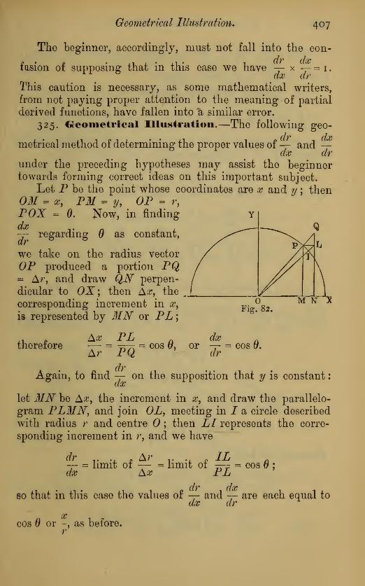
Geometrical Illustration* 407
The beginner, accordingly, must not fall into the con-dr dx
fasion of supposing that in this case we have — x -— = 1
.
ax arThis caution is necessary, as some mathematical writers,
from not paying proper attention to the meaning of partial
derived functions, have fallen into a similar error.
325. Geometrical Illustration.—The following geo-
dr dxmetrical method of determining the proper values of— and —
ax arunder the preceding hypotheses may assist the beginnertowards forming correct ideas on this important subject.
Let P be the point whose coordinates are x and y ; thenOM = x
}PM = y, OP = r,
POX = 0. Now, in finding
— regarding 9 as constant,
we take on the radius vector
OP produced a portion PQ= Ar, and draw QN perpen-
dicular to OX; then A#, the
corresponding increment in x,
is represented by MN or PL;
Fig. 82.
therefore — = ^r^ = cos 0, or -7- = cos 9.Ar PQ dr
Again, to find — on the supposition that y is constant
:
let MN be A#, the increment in x, and draw the parallelo-
gram PLMNy and join OL9meeting in / a circle described
with radius r and centre ; then LI represents the corre-
sponding increment in r, and we have
-7- = limit of — = limit of —^ = cos 9 ;
dx A# PLdr dx
so that in this case the values of — and — are each equal todx dr
xcos 9 or -, as before.
r

408 Change of the Independent Variable.
dvThe values of —^ &c. can also be readily represented
geometrically in a similar manner.
326. Linear Transformations.—If we are given
x = aX + 6F+ eZ, y = a'X + b'Y+c'Z, s = d"X+ b"Y+ c"Z, (20)
then any function V, of x, y and z, is transformed into afunction X, F, Z\ and, as in Ex. 2, Art. 98, we have
dV=
dV ,dV „dVdX dx dy dz
'
dV dV v dV 7„dV
dY dx dy dz
dV^ d_V ,dV „dVdZ dx dy dz
'
Again, proceeding to second differentiation, we get
d*V d( dV ,dV „dV\ ,d(dV ,dV „dVa—\a—+a -^- + a —- + a — [a— + a -—- + adX2 dx\ dx dy dz J dy\ dx dy dz
„d( dV ,dV „dV+ a -7- a-j— + a — + a —
dz\ dx dy dz
2d2 V , d2 V „ d2 V „ , d2 V
= a — + 2aa -—7-+ iaa -
—
r + za a —
—
dx2 dxdy dxdz dzdy
,2d2 V „J
2 Vdy2 dz2
Similarly we have
d*y ^y m d2 v v^2 y 7/ ,<?y
dY2 dx2 dy2 dz2 dxdy
_.„d2 V .„., d2V+ 200 ——- + 2b b
dxdz dzdy'

Orthogonal Transformation. 409
<pv2d2 v ,2
d2 v „ d*r , d2 rJr%
= c TT + c Tl + c2 — + 2CC —
—
dZ2 dx2 dy2 dz2 dxdy
„d2 V „, d2 V+ 2CC -—- + 20 C -7-7-.
dxdz dzdy
327. Orthogonal Transformations.—If the transfor-
mation be such that
x2 + y2 + z
2 = X2 + Y 2 + Z2
,
we have
a2 + a 2 + a"2 - 1, £
2 + 6'2 + i"2 =1, c
2 + c'2 + c"2 = 1. (21)
ai+a'6' + a"6"=o, ac + a'c'+a"c"=o, bc + b'c' + b"c"=o. (22)
Again, multiplying the first of equations (20) by a, the
second by a , and the third by a", we get on addition, by aid
of (21) and (22),
X = ax + a'y + a"z,
In like manner, if the equations (20) be respectively
multiplied by byb\ b'\ we get
Y=bx + b'y + b"z;
similarly,
Z=cx+ c'y + c"z.
If these equations be squared and added, we obtain
a* + V + & - 1, a'2 + V* + c* = 1, a"2 + b"% + c"
2 = i. (23)
aa'+bb'+cc' = o, aa"+ bb"+ cc"= o, a'a"+b'b"+c'c"=o. (24)
Hence in this case, if the equations of the last Article beadded, we shall have
cPV d*V (PV_d*V d?V d?Vda?
+dtf
+dz'
~~ dX>+dY 2
+dZ* ^5 '

4io Change of the Independent Variable.
The transformations in this and the preceding Article
are necessary when the axes of co-ordinates are changed in
Analytic Geometry of three dimensions ; and equation (25)
shows that, in transforming from one rectangular system to
d2 V d2 V d2 V.another, the value of the function -7-=- + -7-7- + -77 is un-
dx2 dy2 dz2
altered.
328. General Case of Transformation for TwoIndependent Variable*.—Suppose that we are given the
equations
a = 0(r, 0), p = *P(r, 0), (26)
then any function of x and y may be regarded as a function
of r and 0, and we have, from (9),
dV dVdx dVdydO ~dx~ d6
+dy Iff
dJT_dVdx dVdydr dx dr dy dr
where the values of -^, ~. —, — can be determined fromdO dv dr dr
equations (26).
Whenever these equations can be solved for r and 0,
separately, we can determine, by direct differentiation, the
values of — , — , —, — , and hence, by substituting in (13),dx dy dx dy
we can obtain the values of -7- and — •
d* dy
When, however, this process is impracticable, we can ob-
tain the values of —, — , &c, by solving tor — and —dx dy J & dx dy
in the preceding equations.
Thus we obtain
dVdVdy^dVdj
—- d9 dr dr dOm
/2-\
dx dy dx dy
dOdr~' drdO

Transformation for Two Independent Variables. 4 1
1
dVdx _dVdxdV d$ dr ~d7dQ
dy dx dy dx dy'
drdd'Mdr
(28)
d2V d2 VThe values of -r-r , tt > &c., can be deduced from these :
dx* dy2
but the general formulae are too complicated to be of muchinterest or utility.
329. Concomitant Functions.—We add one or tworesults in connexion with linear transformations, commencingwith the case of two variables. We suppose x and y changedinto aX + 6Fand a'X + b'Y, respectively, so that any func-
tion (p (x, y) is transformed into a function of X and Y : let
the latter be denoted by </>i(X, Y), and we have
0O*,y) = 0i(X, Y).
Again, let x and y be transformed by the same substitu-
tions, t. e.,
x' = aX' + bY\ y' = a'X'+b'Y';
then since x + kx = a{X-\ kX) + b(Y + IcY),
and y + ky' = a\X + kX) + b'(Y+ kY),
it is evident that
(<* + **', y + ky') =(l>
l{X+kX', Y+kY').
Hence, expanding by the theorem of Art. 127, andequating like powers of k> we get
dx y dy dX dY y v v/
&c. &c. (30)

412 Change of the Independent Variable.
Accordingly, if u represent any function of x and y, the
expressions denoted by
dx
,d\ ( ,d , rf\»J
dy) \ dx J dy) ' '
are unaltered by linear transformation.
Similar results obviously hold for linear transformations
whatever be the number of variables (Salmon's Higher Algebra,Art. 125).
Functions, such as the above, whose relations to a quantio
are unaltered by linear transformation, have been called con-
comitants by Professor Sylvester.
330. Transformation of Coordinate Axes.—Whenapplied to transformation from one system of coordinate
axes to another, the preceding leads to some importantresults, by applying Boole's method* (Salmon's Conies,
Art. 159).
For in the case of two dimensions, when the origin is
unaltered we have
x'2 + 2x'y' cos o> + y
2 = X" + 2X'T cos Q + F'2, "(31)
where to and Q, denote the angle between the original axes
and that between the transformed axes, respectively.
Multiply (31) by A, and add to (30): then denoting
(p(x, y) by u, and <j>i(X, Y) by XI we get
Now, suppose A assumed so as to make the first side of
this equation a perfect square, it is obvious that the other
side will be a perfect square also. The former condition
gives
(d2u .\f(Pu .\f(Pu ,V
fe+MW + \)H^"fAC0SW
J'
* I am indebted to Prof. Burnside for the suggestion that the equations of
this Article are immediately obtained by Boole's method.

Transformation of Coordinate Axes. 413
x o • o a (<?u d2u d2uor A2 Sin2w + A — + -7-y - 2—— cos w
\dx2 ay* dx dy
d2ud2u ( <Pu Y_do?
2<^/
2 \dxdyj
Accordingly, we must have at the same time
AWO + A^h-^ -2^^cosa
d2Ud2U f d2U \+
tfX2 tfF2 U^W" °'
Hence, comparing coefficients, we get
<Pti tfw _ / d2u \ 2 (£UcPU__/_rf£
sin2w sin
2Qand
dHi rf1!! d2w d?U d2U d*U
d#2 dy2 dxdy _ dJ£2 rfF2 dXdYsin
2w sin2Q
(32)
.(33)
Consequently, if u be any function of the coordinates of
a point, the expressions
d2u d2u f d2u V d2w cPu cPu
dx2 dy2 \dxdyj ~dx2 dy2 dxdy
sin2w sin2w
are unaltered token the axes of coordinates are changed in anymanner, the origin remaining the same.
In the particular case of rectangular axes, it follows that
(Pu d?u d^ucPu _ / d2u Vdx2 dy2 dx2 dy2 \dxdyj
preserve the same values when the axes are turned roundthrough any angle.

414 Change of the Independent Variable.
331. Implication to Orthogonal Transformation.
—
When the transformations are orthogonal it is easy to extend
the preceding results to three or more variables (Art. 327).
Thus, in the case of three variables, we have
x 2 + y'2 + z'2 = X'2 + F'2 + Z'2
.
Multiplying this by A, and adding the result to the equation
that corresponds to (30), it follows that the expression
/2dft*
dx2+*M$ +xMS' +xHv!s
, , d2u . , d2u2Z X -7—— + 2X ydzdx dxdy
is unaltered by orthogonal transformation.
Next, suppose that X is such that the quadratic function
in x\ y and z' is the product of two linear factors ; then, byArt. 107, we have
d2u d2u
dx2' dxdy
9
d2u
dxdy9
d2u
d2u .
dhi
dxdz
d*u
dydz
dhi
dx dz' dy dz' dz''
+ \
= o. (34)
But, as the transformed expression must also be the productof two linear factors, we have
d?u . d2u (Pu
dx% ' dxdy' dxdz
dhi dhi , <Fu+ X,
dydx' dy" '
' dydz
dhi dhi dhi
dxdz' dydz' dz7+ A
d*U
dX>+ A
>
<PU d2UdXdY' dXdZ
cW d'U' 7vi + *>
tPUdXdY' dY2 ' "' dYdZ
<ru d2u d*udXdZ' dYdZ* dZ 1
+ A
(35)

Orthogonal Transformation. 415
Equating the coefficients of like powers of A, we see that the
expressions
dht d2u d2u
dx2+dy% * dz2 '
dht d2u I d2u \8 d2u d2u f d2
u V d2u d*u
dx2 dy2 \dxdy) dx2 dz2 \dxdzj dy2
dz2
d2u ydydzj'
and
d2u d2udhc
dx2 ' dxdy' dxdi
d2u d2u d2u
dxdy' dy* dzdy
d2u d2u d2u
dx dz' dy dz' dz2
are unaltered by orthogonal transformation.
The first of these results has been already arrived at bydirect substitution (Art. 327).
These results readily admit of generalization.

416 Change of the Independent Variable.
Examples.
dry1
.
Being given y =/ (w) and u = <f>(x) , find — •
2. Hy = F(t)f *=/(«), u = <p{x), find the value of-^.
3. Change the independent variable from x to z in the equation
a:*—;— 2nxz— + a~y — O, where x = -.
<fa?2 dx z
d2y 2(n + 1) dy
4. Transform (I - x2) — - #— 4-
«
2i/ e= o, beingy^ - #— -t- ay s= o, being given x = sin s.
dx dx
5. If x = r sin cos </>, «/ = r sin sin 0, 2 = r cos 0, prove that — = —-,
dr dxdx
where 6 and <p are regarded as umstants in finding — ; while y and z are re
drgarded as constants in finding -—
•
dx
6. If « be a function of two independent variables, x and y, which are
connected with two other variables, u and vtby the equations
fi(x, y, u, v) b o, f2(x, y, «, v) «o;
show how to express — and— in terms 01 -— and— •
dx dy du dv
7. Transform the equation
d2y 2x dy ydx2 1 + x2 dx (I + xY *
into another in which is the independent variable, supposing x = tan 0.
Am. — + y = o.

Examples. 417
8. If z be a function of x and y, and w = px + #y - js, prove that whenp and q are taken as independent variables, we have
du du dlu d2w dhi
dp "' dq " dp2 rt-*~ dpdq rt-*-' dq 2 rt - s2'
where p y q yr, s, t denote the partial differential coefficients of z, as in Art. 304.
9 If the equation
dHy dn~ ly dyXn -~ + A\X»- 1—-. + . . . + ^n-l# / + An m O
/XT'* /xr'*_1 //'r^' ^be transformed to depend on 0, where x = e0, prove that the coefficients in thetransformed differential equation are all constants.
10. Given x =
d*y
% .-$&.-»-
ay t F(t)
*(t)M) -*{*)*„ )
F(t), F'(t), F"{t)
<p{t), f(o, *"(<)
+(0» fW. *"M
3B

( 4i8 )
3 + 13 + 23 by V 2.
CHAPTER XXIII.
SPHERICAL HARMONIC ANALYSIS.
332. It is proposed in this chapter to give a brief discussion
of the differential equation
tPV d*V cPV^ + ^ +^ = °' (,)
an equation which occurs so frequently in physical investi-
gations. We shall denote the symbolic operator
dx2 dy2dz*
Adopting this notation, we readily see that
9/ x , . fdudv du dv du dv\ , v
V>t<) = u^v + vVu + 2 f——+——+--). (2)
Again, since — (rm )= m#rm~2
,
d2
we have — (rm ) = mrm~2 + m (m - 2) x2>m_4
,(XX
and we readily get
V 2(rm)
= m(m + 1) rm~2
. (3)
Hence, from (2), we have
V 2(rm V) = rmv 2 V+ m (m + 1 ) rm
~2 V
m J dV dV dV\, x+ 2tnrm
-2 [x-— + y — + 2 -5- . (4)
Moreover, if Vbe a homogeneous function of the wf* de-
gree in x, y, z, we get, by Euler's theorem of Art. 98,
V 2{rm V) - r
wV 2 r + w (w + 2 w + 1 ) rm"2F. (5)

Solid Harmonic Functions. 419
333. Solid Harmonic Functions.—Any homogeneousfunction in x, y, z which satisfies equation ( 1
) is called a solid
spherical harmonic function, and frequently a solid harmonic.
We shall denote a solid harmonic of the nth degree byFn, in which the degree n may be positive or negative, in-
teger or fractional, real or imaginary.
It is evident that any constant multiple of an harmonic is
also an harmonic of the same order.
From (5) it follows that a solid harmonic of the nth degree
satisfies the equation
V* (rm Vn ) = m (m + in + 1) rm~2 Vn . (6)
Hence we see that if Vn be a solid harmonic, -r-77 is also
a solid harmonic, whose degree is - (n + 1).
Again, from (3) we see that - is a solid harmonic of the
degree - 1 . Also it can be readily shown that - is the only
function of r that satisfies equation (1). For by (19), Art.
323, we can transform that equation into
-(dr\
idV\ 1 d ( . a dV\ 1 d'V
, ,
dr J+
sin 6 dd \Sm
dO J+
sins dp
dr\ dr
)
Hence, if V be a function of r solely, we must have
do. This gives V in the form - + b.
In like manner, if Vhe a function of the angle <j> solely,
d2 Vit must satisfy the equation -— = o : this leads to V= a<j> + b.
Hence we observe that tan'1( - ] is a solid hannonio of the#
degree zero.
Again, if jFbe a function of solely, we have
^(8in0^) =0,
2 E Z

420 Spherical Harmonic Analysis.
Hence we see that log f tan -J
satisfies the equation
(V 4- z\\7
2 V= o, and we infer that log I
J
is a solid harmonic.
r 4- x r 4" ij
In like manner, log and log are also solid har-° r - x r - y
monies.
It is readily seen that </> log tan(-
)satisfies equation (7)
;
2
hence we see that
tan-1 - log -r + z
x r - z
is a solid harmonic, of zero degree.
If V satisfies equation (1) it is seen immediately that
— ,-— , and —- also satisfy it, as also the general expres-
sion -, in which p y q> r are any positive integers.
Hence, from any solid harmonic, a number of others can
be immediately deduced by differentiation.
dVn .
Again, since -7-^ is a harmonic of degree n - 1, it follows(IX
I (IVn .
from (6) that -r—:;-7— is also a solid harmonic, whose degree
is - n: and so on.
For example, any expression of the form .
k—
xI -
J
is a solid harmonic, whose degree is - (J+ k+ /+ 1).
Examples.
I . Find the condition that
ax2 4- by 1 + ez2 4- <£ry 4- ezz 4 /y«
should be a solid harmonic. ^n«. a 4- b 4 c = Q.
Complete Solid Harmonics. 42
1
2. Prove that
x x . y ,,** + «z tan-1 -, and z log 2r
%r+z y
r (r 4 z)* x* r - z
are solid harmonics.
3. If Vo be a solid harmonic of degree zero, prove that r2u~ l —-— is also ar dxn
solid harmonic.
tt *sin nd> d^tr2"- 1
) . . ^4. Hence prove that — — is a harmonic function.
(a;2 + y
2)2
For, let To = tan" 1( -
J; then, since y - x tan <p f
it can be shown, as in
Art. 46, that
£( teni)=(-')"L^sin nd>
1
Hence is a solid harmonic, as also any function derived from
(*• + y2f2
it by differentiation.
r2 Vn5. Prove that u = — -« is a solution of the differential equation
2(2W + 3 )
v2« - rn.
334. Complete Solid Harmonics.—A solid harmonicthat is finite and single valued for all finite values of the co-
ordinates is said to be a complete harmonic. It can be proved,
by aid of the Integral Calculus, that every complete solid
harmonic is either a rational integral function of the coordi-
nates, or is reducible to one by multiplication by some powerof r. Assuming this, it follows that the number of indepen-dent complete harmonics of degree n is 2/1+ 1, when n is
positive.
For it is readily seen that the number of terms in Vm a
rational homogeneous function of the nth degree in x. y> z, is
(n + 2) {n + 1)- ; and also the number of terms in V 2 Vn is
2
ti (ft ~— 1
1
; hence, since V 2 Vn s o identically, we must have
n In - 1
)
. . .
linear equations connecting the coefficients in Vn ;
consequently, the number of independent constants is
In + 2) (n + 1) n (n - 1)— 2 ', or 2n + I.

422 Spherical Harmonic Analysis.
It can now be shown that every complete harmonic can be
deduced from - by differentiation.T
For the solid harmonio
dx>dyk dz l {x2 f sr + s3)*'
when the differentiations are performed, is readily seen to be
a fraction of which the numerator is a homogeneous func-
tion of the degree n, and whose denominator is -^7, where
11 k + J + /. If this function be represented by -^, the
numerator F«, by (6), is also a solid harmonic.
We can now show that the number of independent har-
monics of degree n that can be thus derived is in + 1.
For, since
dz2 \r) " \dx2+
dy 2
) \r}we see that
dz2m \r) K ] \dx2 dy2
) \rf
( d% d2\m
in which f—- + —
]can be expanded by the binomial theorem
as if— and— were algebraic quantities, and the resultingax ay
differentiations of - taken.r
Hence, if / be even, we have
1 1
dx>dyk dzl \r) " '" *' dx> dyk \d^2+dy2
) \7/
and, if I be odd,
dxQy1^1 \r)~^l' dx* dy
k \dx2+dy2
) dz \ rj

Spherical and Zonal Harmonics, 423
Accordingly, in the former case, we get a number of terms
d?¥q 1 1 \each of the form -——
- - , where p + q = n ; and in the
latter, terms of the form - „ . - \-r ( - )> , in which p + a = n - 1
.
Now there are p + q + 1 , or n + 1 terms in the former case,
and n in the latter. Hence there are in + 1 independentforms, as was to be proved.
335* Spherical and Zonal Harmonics.—If a solid
harmonic Vn be divided by rn , the quotient may be regarded
as a function of the two angular coordinates, or spherical
surface coordinates, 9 and </>. Such a function is called a
spherical surface harmonic of the degree n.
Hence, if Vn = rnYn , then Yn is a spherical harmonic of
the nth degree.
It is obvious that the general spherical harmonio of the first
degree is of the form a cos 6 + b sin 6 cos </> + c sin sin <£, wherea, 6, c are arbitrary constants. Also, the general expression
for Y2 can be written down readily (see Ex. 1, Art. 333).Again, by (19), Art. 323, we see that Yn satisfies the
differential equation
d ( . a dTn\ 1 <?Ynsin d0 \ tf0 7 sin
2dxf>
This equation admits of a useful transformation : for, let
jut = cos 0, then, since
we get
Again, if a spherical harmonic be a function of solely, it
is called a zonal harmonic. Hence, if Pn be a zonal harmonic
of the nth order, it must satisfy the equation
£{(l ^£-} + ,(„ +1)P.-a do)

424 Spherical Harmonic Analysis.
When n is a positive integer, the value of Pn can be readily-
represented by a finite series. For since, by hypothesis, Pn
is a function of the nth degree in ju, we may assume
m-n
Pn = S {am »'•').
m=o
dPHence —- = 2 (mam jui
m~ l
) ;dp
•"• -r-(i "i"2) -r1' = 2w(m - i)am u
m-*- 2m(m + i)tfm /uM
.
djj. dp
Substituting in (10), and equating the coefficient of f±m to
zero (since the result must vanish identically), we get
(m + i) (m + 2) tfm+2 == - (n - m) (m + n + 1) tfm .
Hence, observing that the highest power of ju is n, wehave
n(n-\)dn-2 = - an — r, <&C,
2 (2W - I)
and we may write
n (1
2 (2
n^)_ «(.-i)(»-2)(W_-3} )
2«-l)^ 2.4(2n- l)(2W~3))
(»)wliere r/w is an arbitrary constant.
This is the general form of a zonal harmonic of integer
positive degree ; and we see that two zonal harmonics of the
same degree can only differ by a constant multiplier.
It can be shown independently of the above that
d \n—J
(jit2 - i)
wsatisfies the equation (10).
In order to prove this we shall assume u ** /** - 1 , and
write the symbol 1) for — ; then we have to prove that
D {uDnn (un)} - n (n + 1) D" (un) = o.

Zonal Harmonics. 425
till
Now, observing that — = 2/x, we get, by Leibnitz'sdp
theorem of Art. 48,
+ w(n+ OD"-1 ^'*).
Again, since
D(un+l) = 2 (rc + i)^mw
,
we have
Dn"(un+1)= 2 (n + 1) Dn
(iuiin)
- 2 (» + 1) /iDn
(t*n) + 2^ (» + 1) D*" 1 (wn ).
Equating these values of i)7i+1 (ww+1 ), we get
uDu+ l
(**) - ft (ft + 1) I)91- 1 (u
n) ;
hence D {uDnn (nn)
) - n (n + i ) Dn (un ) = o. (12)
Consequently l)n (un ) satisfies the equation in question.
Hence we infer that
P- - C(0<"' - "'
The student can verify, by direct differentiation, that
this expression differs only by a constant factor from the
value of Pn found in (11).
It is usual to assume that Pn is that value of the pre-
ceding expression which becomes unity when fx = 1
.
To find this value, we have
= 2«ju(jPj' V - I)-* + 2n (» - ( -T- ) </*' " O"-',
by Leibnitz's theorem.

426 Spherical Harmonic Analysis.
I $ \ n-2
Now it is readily seen that f—j
{u2 -
1)
n_1 = o when yu = 1;
hence, when u = 1, we have
(fiTo*-*—(STV-on-i
= 22«(w - (jYV - O""
1* &e.
Consequently, when /u = 1
,
and we have
'•-^sCfifr' -> (,s
The foregoing result can be readily shown in another
manner. For 2[nl— ) (u
2 - 1)
nis the coefficient of hn in the
expansion of (1 - 2uh + A2)-* (see Ex. 6, p. 155).
Again
((# - a)2 + 3/
2-»- s
2)"* = (r2 - 2#r/z + a2
)
= - (1 - ha + A2)"*, where A = -,
_ 2 _^_l.(-Y^-.)»-
in which we suppose a > r.
But V*{(* -«)* + »* + *")"* -o;
hence
•*• v,K^" ij")" o;
[— )(u2 - i)
n satisfies equation (10), &o.
The functions Plf • . . Pn are usually called Legendre's
Coefficients.

Complete Spherical Harmonics. 42
7
Examples.
1. If /i = I, prove that P« = I for all values of n.
2. If fx «= - I, prove that P„ = (- l)».
3. If (x < I, show that the series
Pi + P» + . , . + P» + . . .
is convergent.
4. Prove the relations
P4= g , P* = g-
5. Prove the equations
— (Pnf i - Pn-l) - (2H l)P„,
(« + l)P-+ i- (2>* + O/i/'* + /*PM_i = O.
336. Complete Spherical Harmonics.—From Art. 334 it follows that a complete spherical har-
monic Yn of the nth order, when n is an integer, contains
in -f 1 arbitrary constants. Its value can be expressed byaid of the corresponding zonal harmonic Pw , as we prooeed
to show.
Since Tn is in this case a rational integer function oi
sin $ cos </>, sin 6 sin <p and cos 0, we may suppose it expressed
in a series of sines and cosines of multiples of <£, whose coef-
ficients are functions of #, or of fx. We accordingly assumethat Yn consists of a number of terms each of the formM8 eoss0; then, substituting in equation (8), and observing
. . . d2cos *(b . , . . * . , i i
that —2
= - a* coss^, we obtain, on equating to zero the
coefficient of cos $0,
^|(l^^rrv +w(w+i)^ =o
-(I4)
If, as before, we write u for jx2 - 1 , and 2) for -7-, this
dfj.
becomeswD{wZ)i!f,)-62
ilf, -w(n+ i)wiI/, = o. (15)

428 Spherical Harmonic Analysis.
s
Now, let M8 = u 2v ; then
f s
uDHf8 = u2 Dv + sjmifv;
therefore , 8 8 9
uD (uDMs) - u2*D2v + 2 (s + 1 )
^aTDv + su2"v + iVVtV«
Substitute in (15), and divide by w2; then
uD2v + 2 (s + 1 ) juDt? + [s (9 + 1 ) - w (n + 1 )
} v = o. (16)
It is readily seen that this equation is satisfied by assum-ing v = D*Pm ; for substituting this value for v in (16), it
becomes
uD*2Pm + 2 {9 + i)M 7)*+1Pm + * (« + 1 ) Z)*Pm-»(•+ i)D°Pm = o;
but by Leibnitz's theorem the first three terms are equivalent
to Dsn (uDPm ) ; whence the equation becomes
B* 1 {uDPm ) -n(n+i)DsPm = o.
But this equation follows immediately from (10) bydifferentiating it s times with respect to /i.
Accordingly, the expression
satisfies equation (14), and hence
G08s<l>(S-if(J-)*Pn
satisfies (8).
T i-i <tf*(sin$0) .,
In like manner, as— r = - s2 sin s0, the expression
d(j)
ri^^-o^iyp.also satisfies the same equation.
Accordingly, equation (8) is satisfied by the expression
(^,008*0 + A sin «0) (/I1 - lylj-UPn), (17)
in which ^4, and Bt are arbitrary constants.

Laplace's Coefficients. 429
This expression is called a Tesseral Surface Harmonic, andis said to be of the degree n and order s.
If we give all integer values to s from 1 to n9the com-
plete spherical harmonic Yn can be written in terms of
Tesseral harmonics as follows :
—
Ld*PnFn = ^( Pn + 2 (A s eoss<f> +
B
8 sin s<t>)(iu2 - i)
? tt, (18)5=1 Cl
fX
( d \n
in which (-7-) (/n2 - i)
n may be substituted for Pn if neces-\dfxj
sary.
This equation contains the proper number 2n + 1 of arbi-
trary constants, and consequently may be regarded as a
general expression for a complete spfygrical harmonic of in-
teger positive degree.
There is no difficulty in showing by differentiation that
d \w+*— ) (fx2 - i)
n differs only by a constant from
A* / \ A*2[2n- 1)
[n - s) (n - s - 1 )(n - s - 2) (w - s - 3)
2.4. (2W - i) (2tt - 3)+ — —— /i
n-5-4 + &c.
Hence that part of Yn which depends on the angle s<p maybe written
(1 - ii)2Un-- {
n ~ s
^n~^~ l
\n-*-* + &cA {A 8 cos scp + B9 sinsft).
This agrees with the general expression given by Laplace(Mecanique Celeste, tome in., chap, ii., p. 46).
337. Laplace's Coefficients.—It is immediately seen
that the expression — 7^—7 7^—;
ttttt satisfies the{(a?
-
x) 2 + (y - j/)1 + (* -a) 8
}*
general equation (1), as also the corresponding equation
rfT cPV d2 Vdx 2
+<fy'
2+
dz 2 ~ °*

430 Spherical Harmonic Analysis,
Transferring to polar coordinates, the preceding expression
may be written (r2 - i\rr + r 2
) , where
x' = r sin 0' cos 0', y' = / sin ff sin <p\ z = r cos 0'
;
and A = cos cos 9' + sin sin 0' cos (<£ - <p')
.
If P and P' be the points whose coordinates are xyz and#'#V, respectively, then
i i / , r' r/2Y* i / . r r2
, = - I - 2A - + — = - I - 2A — + -7-
PP r \ r r'J r \ r r 2
Accordingly, if
( i - 2AA + h2)-% = i + Lxh + LJi2 + . . . + Lnh
n + . . .,
we have
and
i i L,r L^r"i
. when r > r
i i Zir X3 (
2
PP' ~r' ' r'
2r'
3+
'"
P„r», when r < r
Hence, since V 2( -p-p ]
= o, we must have V 2(-~[
)o,
and also V 2 (Lnrn
)s o.
From this we see that Ln is a spherical harmonic of the
degree n, and that it satisfies the equation
d ( , .. dLn ) i d?L
d/j.(l -rti?) +
irrfsW + ttiH + l)Ln =
The functions Lu X2 , . . Ln are called Laplace's Coef-
ficients, after Laplace, to whom their introduction into
analysis is due.
The value of Ln may be deduced from that of Pn in (i i)
or (13), by substituting pix + </i - /u2 y/ 1 - jx
2 cos ((p - <p') in
place of /x, where /u = cos 6, and jjl == cos 0'. Hence it is a
function of the nth degree in /x, y/ 1 - u2 cos and </ 1 - fi
2 sin;
as also in 1/, \/ 1 - p.'2 cos 0' and </i - /u
2sin f\

Laplace's Coefficients. 431
Moreover, since Ln is a spherical harmonic of the uth
degree, and symmetric in ji and //, as also in <p and <^', it
must, by (18), be of the form
*=» i LdsPn dsP*'Ln = a PnPn+Z_
i
a9 oos8 (£-0')(/if-i)» (iu'
2-i>— __f
in which the coefficients #<>, «i, ...«#.. . are constants, the
values of which remain to be determined.
It is immediately seen that a = 1 : for if jul = 1 , we have
Pnf = i, and Ln - Pn .
In the Integral Calculus, Art. 233, it is shown that
%s = (- 1)*L Assuming this result, we have
*="In - 5 * * d5P„ rf'Pn
Some further applications of spherical harmonics will befound in the Integral Calculus, Arts. 230-5, but for a morecomplete treatment of the subject, which involves the applica-
tion of Multiple Integrals as well as the solution of Differential
Equations, the student is referred to Thomson and Tait's
Treatise on Natural Philosophy ; to Ferrers' Spherical Har-monics; or to Todhunfcer's Treatise on Laplace's, Lamp's, andBessel's Functions.

432 Spherical Harmonic Analysis.
Examples.
I. If u be a solution of the differential equation
du du du ... . _ . .
prove that x I- y -7- + *— w"l a^so oe a solution of it,r dx dy dz
2. Show that each of the quantities
- - /a2, (1 -/x2
) cos 20, (I - fi2) sin 20, ph-p? cos 0, /4V7 1 -/x 2 sin
is a surface harmonic of the second degree.
3. Prove that the expressions
r+ z r r+§ z . r + z 2rxzz log 2r, log— -, x log + —
r - z / r - z r3 r - « #2z a;2 4- y
2
are solid harmonic functions.
4. If the polar variables be replaced by u and v, where
cot -el(*> = u. tan - e^ = v % and i = V - 1,
2 2
prove that any surface harmonic of the order n satisfies the equation1
d2 V n(n+ i)Vdudv {u 4- v) 2
5. If p1
, pi2, pz2 be the roots of the equation in A.,
x%y
l z2
I= —
+
\ \ - A2 A - k2 '
and if
, __dp
, <h\M ~ 1{f-V)if-*f
Ul ~ ^(h2 - pi2)(pi
2 -K2)'
dp2duz =
prove that
d2v d2 v d2v\-
\= o
dx2 dy2 dz2
transforms into
d2v d2v dtv(p* - pi*) J~% + (p* - p,») -r-, + fp,» - p») -

( 433 )
CHAPTER XXIV.
JACOBIANS.
338. JTacobians.—The results obtained in Articles 330and 331 are particular cases of a class of general theorems
in determinants which were first developed by Jacobi (Crelle's
Journal, 1841).
Thus, if w, vyw be functions of x, y, s, the determinant
</-
du du du
dx~' dy 1%
dv dv dv
dx* dy' ~d!
dw dw dw
dx~9
d~y' dz
(I)
was styled by Jacobi a functional determinant. Such a
determinant is now usually represented by the notation
d(u, t\ w)
d(x, y, z)'
and is called the Jacobian of the system uyv, iv with respect
to the variables #, y, z.
In the particular case where u, v, w are the partial diffe-
rential coefficients of the same function of the variables x, y, z,
their Jacobian becomes of the form given in Art. 331, and
is called the Hessian of the primitive function. Thus the
determinant in Art. 331 is called the Hessian of u, after
Hesse, who first introduced such functions into analysis, and
pointed out their importance in the general theory of curves
and surfaces.
2F
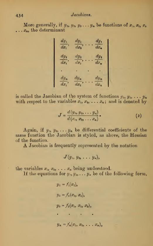
434 Jacobians.
More generally, if yly y2 , y*. . . yn bQ funotions of xl9 x2 , x*
. . . xn9 the determinant
dyi
dxi'
dy%
dx* '
dyi
dxn
dy2 dy% dy2
dxi dx2'
' dxn
•
dyn
• •
dyn dyn
(IX \ (XX^ dxn
is called the Jaeobian of the system of functions v/„ y2y . . . ynwith respect to the variables x i9 x2 , . • . xn ; and is denoted by
J*d(yl9 y2,...yn)d(x l9 x2 , ...xn)
(2)
Again, if y X9 y2 , . . . yn be differential coefBcients of the
same function the Jaeobian is styled, as above, the Hessianof the function.
A Jaeobian is frequently represented by the notation
J(yi> y*> • • • yn),
the variables xu x2j . . . xn being understood.
If the equations for yu y2y . . . yn be of the following form,
yi - /i(«0,
1/2 = /2 (#1, «*),
2/n—
./"»»(#!> ®2y • • • #«/>

Examples. 435
it is obvious that their Jacobian reduces to its leading term,
viz.
dyx dy2 dyn , ,
J T"" • rr~ • • • ~r~#
(3)a^i dx2 dxn
This is a case of a more general theorem which will be
given subsequently (Art. 343)-
Examples.
1. Find the Jacobian of y\> y2 , . . . t/n, being given
yi = 1 - x\, y2 = x\ (1 - *a)f Jte = #1*2 (1 - #3) . . .
y,» = #i#2 . • . xn .\ (I - #»). -4w*. /= (- i)"^"" 1^""2. . . #«-i.
2. Find the Jacobian of x x , #2, . . . #>» with respect to 0i, 02, . . . 0», being
given
#1 = cos 0i, X2 = sin 0i cos 2 , #3 = sin 0i sin 02 cos 03, . . .
xn = sin 0i sin 2 sin 3 . . . sin 0,4-i cos 0„.
d(x\. x%% . . . xn) ... . ,
Ans. -j—9-—-
[ = (- i)'» sinM 0i . sm'»- ,
2 . . . sm0M .
"(01, 02, ... 0m)
339. Case where tbe Functions are not Indepen-dent.—If yu y2 . . . yn be connected by a relation, it is
easily seen that their Jacobian is always zero.
For, suppose the equation of connexion to be represented
by
F[yu tf%, . • • y») - o 5
then, differentiating with respect to the variables #„ x2, . . . xmwe get the following system of equations :
—
dF dy x dF dy2 dF dyn
dyxdx x dy2 dxx dyn dx x
2 F2

436 Jacobians.
dF dyx dFdy2 dF di/n
dy x dx2 dy2 dx2 dyn dx2
dF dyx dF dy2 dF dyn
dyx dxn dy2 dxn dyn dxn
. .. . ,. dF dF dFwhence, eliminating -—
,—- . . .
—— , we get6 dy: dy2 dyny *
d{yuij*,...yn) = Q,.
d (xx , x2 , . . . xn ) ''
The converse of this result will be established in Art. 344 ;
and we infer that whenever the Jacobian of a system of
functions vanishes identically the functions are not indepen-
dent. This is an extension of the result arrived at in Art.
3H.
340. Case of Functions of Functions.—If we sup-
pose f#i 9u2y uz to be functions of t/h y2y y3 > where y Xy y2 , y3 are
functions of xu x2 , x3 ; we have
dn x dui dy x du x dy% du x dy-.
dx xdy x dx x dy2 dxx dy3 dxx
'
du x du x dy x du x dy2 duxdyz
dx2 dy x dx2 dy% dx2 dy3 dx2
'
du x du x dyx
du x dy2 du x dy3
dxs dy x dx3 dy2 dx3 dyz d.r3
'
&c.

Case of Functions of Functions. 437
Hence, by the ordinary rule for the multiplication of
determinants, we get
dui dux du x du x du x du x dyx dyx dyx
dx2 dxz Wx dy2 dy* dx' dx2 dxz
du2
dxx
du2
dx%
du2
dxz
=du2
dffi9
du2
dy*'
du2
dy*•
dy2
dxC
dy2
dx2
dy2
dx-*
du3 dih du3 du3 du3 duz dy* dy* dy*
dxx
f
dx>i dxz dyt dyl dy dxx' dx2 dxz
ajh ujh / x
ordjiix, u2y ih) d(u l9 u29 ih) d{y l9 y29 y3)
d{xx, x2 , x3) d(y l9 y29 yz )' d(xl9 x2 , <r3)
It follows as a particular case, that
d(y\, y*> y») d(x l9 x29 xz )
d(xl9 x29 x3) d(;y l9 y2y y»)(6)
These results are readily generalized, and it can be shownby the method given above that
d(u l9 u29 . . . un ) d(u l9 u29 . . .un) d(y l9 y29 . . . yn )
d(xl9 x2 , . . . xn ) d[yl9 y2 , . , yn )' d(xl9 «*»,•.. xn)' (?)
This is a generalization of the elementary theorem of
Art. 19, viz.
Again,
du du dy
dx dy dx
djyxy y2 , . . yn )d(x l9 x29 . . . xn )
d(x]9 x29 . . . xn )d(yl9 y29 . . yn )
= 1. (8)
This may be regarded as a generalization of the result
dx dy
dy ' dx

438 Jacobiam.
341. The Jacob!an is an Invariant.—In the parti-
cular case of linear transformations we have a system of
equations as follows:
—
y x= a xxx + a2x2 + anxn9
y2 = b xx x + b2x2 + bnxn9• •••••
In this case
d\ Ct2 • • • (In
d{V\, Vl Vn)
d{xl9 x2 xn )
b x b 2 . . . bn
l\ l2 . . . /
„
This determinant is a constant, and is called the modulus
of the transformation.
Accordingly, in linear transformations the transformed
Jacobian is equal to the original Jacobian multiplied by the
modulus of the transformation.
In the case of orthogonal transformation (see Art. 327)the modulus of the transformation is unity, and accordingly
the Jacobian is unaltered by such a transformation.
342. Jacobian of Implicit Functions.—Next, if
u 9 v9w
9instead of being given explicitly in terms of x
9 y 9z
9
be connected with them by equations such as
Fx(x,y 9z,u
9v
9w) = o, Ft{z9y,z,u,v,w) = Oi F%(x 9
y,z,u,v,w) = o9
then u9 v, w may be regarded as implicit functions of x
9 y 9z.
In this case we have, by differentiation,
dFx dFx du dFxdv dF
xdw _
dx du dx dv dx dw dx
dFx dFxdu dFx dv dFx dw— + -7- +
dy du dy dv dy dw dy— = o,
IF* dF, du-r +
dx du dx dv dx
dF2 dv dF2 dw _dw dx
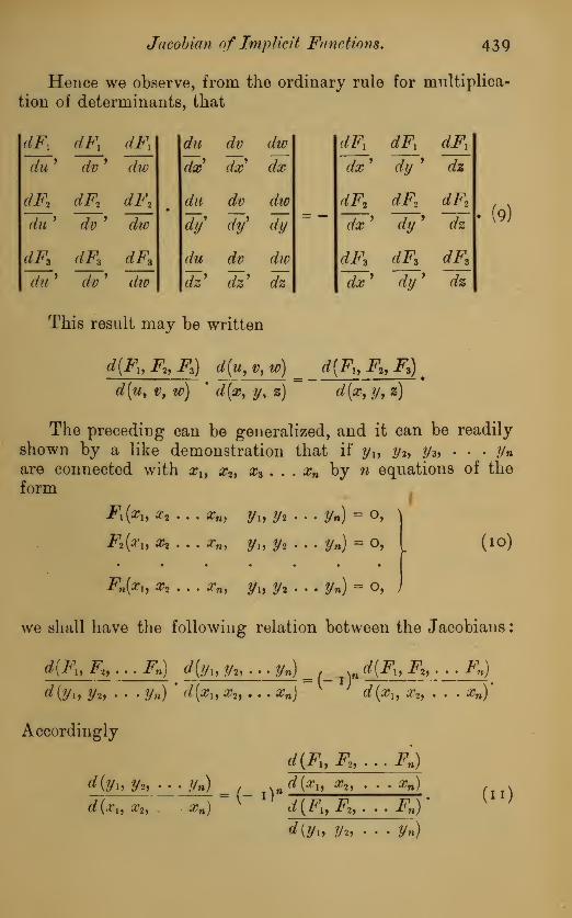
Jacobian of Implicit Functions. 439
Hence we observe, from the ordinary rule for multiplica-
tion of determinants, that
dFx dFl dFx
du' dv' dw
dF3
du'
dFz
dv'
dF2
dw
dF3 dF3 dF±
du dv dw
dx dx dx
du dv dw
dy d? dy~
du dv die
dz9
dz' dz
dFx dFx dFx
dx' dy' dz
dF2
dx'
dF*
dy'
dF%
dz
dF, dF3 dF3
dx dy ' dz
(9)
du ' dv ' dw
This result may be written
d{Fl9 F2y FJ d{u, v, w) _ d{Fu F2y Ft)
d{uy v, w) ' d(xy y, 2)
~ d[x9 y9
z)
The preceding can be generalized, and it can be readily
shown by a like demonstration that if y X9 y 2 , y^ . . . ynare connected with xu x2y x* . . . xn by n equations of the
form
Fx (xXy x2 . . . xn , y ly y2 . . . yn )= o,
F2 (x Xy Xt
.
. . xn9 yXy y2 ... yn) = o,
Fn(xx , x2 . . . xn , yXy y2 . . . yn)= o,
(10)
we shall have the following relation between the Jacobians
:
d(Fl9 F2y ... Fn ) d{y iy y2y . . . yn) d{Fly F2y . . . Fn )
d(y Xj y2y . . . yn ) d[x Xy x2y . . . xn )d(x x , x2y . . . xn)
Accordingly
d{ffiy y*,
d(xi, x2y
d(Fly F2y ... Fn)
• Vn) m <_ )nd{xXy X2y . . . Xn )
xn )
v d{FXy F2y . ..FH)
d(yu ?h, • • • Vn)
(II)

440 Jacobians.
343. Again, the equations connecting the variables are
always capable by elimination of being transformed into the
following shape :
—
(12)
0i (a?ij #2 j • • • #», */l) = O,
02 (#2 j #3, • • • *», y» y%) = 0,
03 (#3, #4, • • • ff*J ?1| #2, £/») - O,
*n(a«, yn 3/2, ... y») = o.
In this case the Jacobian determinant
d(<l>i, 2? . . . <pn)
d{yi, y%> . . . y«)'
as in Art. 338, reduces to its leading term
d(f>i d<j>2 d<j>z d(pn
df/i dy2 dyz' ' dt/n
In like manner,
d(<f>i, 02, • • • </>n)
d(xly x2 , ... xn)
reduces to
dcf>i dfo d(p tl
dx x dx2' ' dxn
Accordingly, in this case, the Jacobian
rf0, d(j)2 d<pn
d{t/» V%> • • - Vn) , y, dxi dzi'
d{xly x2l . . . xn)
x/d<p l d(f)2
' dxn
d<j>n
dy x di/2' dyn
(-3)
344. Case where Jacobian vanishes —We can nowprove that if the Jacobian vanishes, the functions yu y2 ,
. . . ynare not independent of one another.

Case where Jacobian Vanishes. 441
For, as in the previous Article, the equations connecting
the variables are always capable of being transformed into
the shape given in ( 1 2), and accordingly, if J (y\ yl} • • . ytl) o,
we must haved(j>\ d(f)2 d(pn _
dxi dx2"
* dxn
f;hat is, we have —^ 3 o for some value of i between 1 and n.
dxi
Hence, for that particular value of i the function <£,- mustnot contain x* ; and accordingly the corresponding equation
is of the form
<f>i (tijftii • • • Xn% Ply y*> • • • Pi) = O.
Consequently, between this and the remaining equations,
0t+i = 0> </>i+2 = 0, . . . (pn = o,
the variables $i+\ $<«j . • • #n can be eliminated so as to give
a final equation between y Xy //2 , . . . yn alone. This establishes
our theorem.
Also, it follows that if the Jacobian does not vanish,
the functions are independent.
345. In the particular case where
yx- Fx (xu x2f . . . x„),
y* = F2 (yi, x2 , . . . xn),
yn =Fn {yu y2, . . . y*_u xn),we have
d (y/ It ya , • - . ?/») djh dy% dy%^
.
r/ (a?!, ir2 , . . . #n ) ^ * dx2' ' dxn
It may be observed that the theory of Jacobians is offundamental importance in the transformation of MultipleIntegrals (see Int. Calc.
}Art, 225).

44 2 Jacobians.
Examples.
i. Find the Jacobian of yu y2 , . . . yn with respect to r, U 2 , . . . 0„-i,being given the system of equations
—
yx = r cos 0i, y2 — r sin 0i cos 02, y3 = r sin 0i sin 2 cos 03, . . .
yn = r sin 0i sin 6% . . . sin 0„-i.
If we square and add we get
yr + y-i7, + . . . yn
2 - r1.
Assuming this instead of the last of the given equations, we readily find
/= r"- 1 sin»»-20i sin" 3
02 ... sin 0„-3 .
2. Find the Jacobian of yi, y2 . . . y„, being given
yi = #i (i - #2), ^2 = #1*2 (1 - «*) . • .
y»-l = X\X2 • • • %n-\ (I ~ Xn) t
j/n = #1 #2 . • • #m
Here, yi + y2 + . . . yn = X\, and we get
rf(yi, 2/2, .. . yn)
<*(*!, #2, • • Xn)= r,»»-l/»:o»-2
346. Case where a Relation connects the Depen-dent Variables.—If y„ //2 . . . yn , which are given func-
tions of the n variables x ly x2 , . xny be connected by an
independent relation,
F{yi,y%, . . . yn ) = o, (15)
we may, in virtue of this relation, regard one of the variables,
xn suppose, as a function of the remaining variables, and thus
consider yu y2 , • . . yn-\ as functions of xh x2 , . . . #n_i. Inthis case it can be shown that
dFd{y\, /A, » • . yn-i) ^ dyn d{yu yt . . . y»)
d{xu x 2 , . . . #„_!) dF_d(x l9 x%9 . . . xn)
dxn

Case where a "Relation connects the Dependent Variables. 443
For, if we regard xn as a function of xu x2 , &c, we have
dx\W dx
x
+dxn dxx
9dxx
KV2) dx x dxn dx x
'
Also, from equation (15),
dF dFdx„_ dF dF dx^ _ &dxx dxn dxx
%
dx2 dxn dx2
dF dF dF
A . 1 . v aX\ ^ ctx2 . &xn_\Again, let A, - -p A 2 =^p . . . A M-i = -^jr \
dxn dxn dxn
. ctxn . dxn ^ctxn
tnen —— = — Ai, —— = — A 2 , . . .—— = — A n_i.
dxx dx2 dxn_x
Hence ' W -£. X * ' W..^X* 4..
• . . &c.
Accordingly, substituting in the Jacobian
d(yu y2 , . .. yn_ x)
it becomes
a \X\y x2y » • . xn_\)
dy\^
^yi ^L_A ^L --^--A —tf#i flfcn
'
rfr2 ^n' " * ^n_!
n~ d#n
^i_A — -^! -A —
—
rfy>A —
dxx dxn' dx2 dxn ' " r/#n_! flfcn
If this determinant be bordered by introducing an addi-
tional column as in the following determinant, the other

444 Jacobians.
terms of the additional row being cyphers, its value is readily
seen to be
or
dFdxn
dyx dffx
dt/n.i dyn_ x
dxx*
dx>
dF dFdxi
'
dx2
'
dyi
dxx
*
dx2 dxn
dy2
dxx
y
dy*
dx2
dy%
dxn
dyn-i dyn -\ dyn-i
dxif
dx2
'
dxn
K K . . . i
df/i dyx dyx
dxx
*dx2
*
dXn
dy2
dxi
dyt
dx2
'
dy%
dxn
dyn-i
dxn
dFdx„
Again, we have
dF dF dyx dF_ dfr dF dy,
dxi dyx dx\ dy2 dxx
dF dF dy x dF dy2
dx2 dyi dx2 dy2 dx2
dyn dxx
'
dF dyn
dyn dx2
'
Substituting these values in the last row of the preceding

Case inhere a Relation connects the Dependent Variables. 445
the theorem is established, since we readily find that the
determinant is reducible to
dyx d]h dyx
dx\ dx2
9
dxn
dF dy± djh ty_2
dyn chcx* dx2' dxn
dF a • • •
dxndjjn dt/n dyn
dx x
'
dx2
y' dxn
(16)
It may be well to guard the student from the supposition
that this latter determinant is zero, as in Arts. 339 and 344.
The distinction is, that in the former cases the equation
F{t/u yi • • • !/n) = o, connecting the y functions, is deduced
by the elimination of the variables xl9 x2 > . . . xn from the
equations of connexion ; whereas in the case here considered
it is an additional and independent relation.
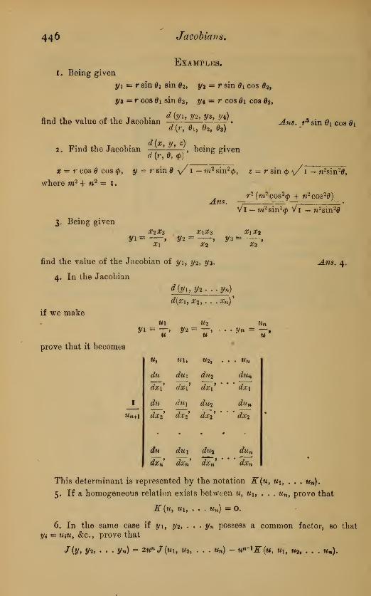
446
I. Being given
Jacobians.
Examples,
yx = r sin 6\ sin 2 , y% - r sin 0i cos 2,
ya = r cos 0i sin 3 , y4 = r cos d\ cos 3 ,
-4ws. r3 sin 0i cos 0ifind the value of the JacobiandJ*
1' ^pJ'l
d{r, 0,, 2 , 3)
_. , , T . . d(x* y, z) .
2. Find the Jacobian —), being given
d(r,d,<p)
x-r cos cos <p, y = r sin y/ 1 — m2 sin2</>, z = r sin <p \/ 1 — n2sm%
where m2 + n2 = I.
r2 (m- cos2(p + «2 cos20)
Vl-w2 sin2<f>Vi - n2sin26
Ans.
3. Being given
#2 #3 X\Xz X\.X%
y* = ~> y* =—•y* = ^
_»
X\ X2 X3
find the value of the Jacobian of yi, y2 , y3.
4. In the Jacobian
d(x l} X2 ,. . .«*)'
^4w*. 4.
if we make
prove that it becomes
u\ U2 un
w, Ml, U2, ... Un
du <£wi diii dun
dx\ Si' dx\ ' ' dx\
I du du\ du2 dun
Wn+1 dxi dX2 dX2* ' ' dX2
du du\ du% dun
di~n dxn dXn "* dxn
This determinant is represented by the notation K(u, u\, . . . ww).
5. If a homogeneous relation exists between u, u\ f . . . wn ,prove that
K(u, wi, . . . u„) = 0.
6. In the same case if yi, y2 , . . . y« possess a common factor, so that
yi - UiU, &c, prove that
J(y* V2, . • • yn) - 2Un J(uh W2 , . . . «„) - ^"^(w, «,, W2, . . . «n).

( 447 )
CHAPTER XXV.
GENERAL CONDITIONS FOR MAXIMA OR MINIMA.
347. Conditions for a Maximum or Minimum forFour Variables.—The conditions for a maximum or a
minimum in the case of two or of three variables have been
given in Chapter X.It can be readily seen that the mode of investigation, and
the form of the conditions there given, admit of extension
to the case of any number of independent variables.
We shall commence with the case of four independentvariables. Proceeding as in Art. 162, it is obvious that the
problem reduces to the consideration of a quadratic expres-
sion in four variables which shall preserve the same sign for
all real values of the variable.
Let the quadratic be written in the form
u = aux2 + a%2x
2 + a^x 2 + aux?
+ 2a l2x xx2 + 2a i3XiX3 + 2a liX lxi + 2a2ix2xZ9
+ 2a2iX&i + 2034^4, (1)
in which an , a l2y a22 , &c, represent the respective seconddifferential coefficients of the function, as in Art. 162.
We shall first investigate the conditions that this ex-
pression shall be always a positive quantity. In this case
#n> «22, #33, &c, evidently are necessarily positive : again,
multiplying by au , the expression may be written in thefollowing form :
—
anti^{anXi^a 12X2 +a^x^a lixi
)
2-¥(ana22 -au
2)x2
2 ^(ana^-an)xi2
+ (#ii#44-#u2)^4
2 + 2(ana 2^-a l2a l3)x2xd
4 2 [anau - a l2au)x2Xt + 2 [anau - a lzau)xzxA . (2)

448 General Condition* for Maxima or Minima.
Also, in order that the part of this expression after the
first terra shall be always positive, we must have, by theArticle referred to, the following conditions :
—
and
#11#22 - #12 > o,
(ana22 - an) (#ii#33 - au2) - (an a2Z
- a ]2an)
2 > o,
#n#22 — #12 #11#23 — #12#13, #11#24 ~~ #12#14
#11#23—
#I2#13, #11#33 ~" #13 , #11#34-#13#U
#11#24~-#12#14> #ll#34"~#13#14> #n#44 ~ #14
> o.
(3)
(4)
(5)
To express the determinant (5) in a simpler form, wewrite it as follows:
—
1
#11
a n> a 12, #13, #14
O, #11#22~#12% #11#23 ~"#ll#13, #11#24 ~ #12#{4
O, #H#23 "" #12#13, #11#33 ~ #U , #11#34 "~ #13#14
O, #11#24 ~ #12#14, #ll#34 ~#1*#14, #n#44 — #14
(6)
Next, to form a new determinant, multiply the first rowby #12, #13, #i4, successively, ami add the resulting terms to
the 2nd, 3rd, and 4th rows, respectively ; then, since each
term in the rows after the first contains an as a factor, the
determinant is evidently equivalent to
#i]
#11, #12, #13, #14
#12, #22, #23, #24
#13, #23, #33, #34
#14, #24, #34, #44
(7)
In like manner the relation in (4) is at once reducible to
the form
#11, #12, #13
#11 #12, #22, #23
#13, #23, #33
> o.

Maxima and Minima, 449
Hence we conclude that whenever the following condi-tions are fulfilled, viz.
#11) #12) #13) #14
#11) #12) #13
an > o,#11) #12
#12) #22
>o, #12) #22) #23
#13) #23) #33
>o, > o, (8)#12) #22) #23) #24
#13) #23) #33) #34
#14) #24) #34) #44
the quadratic expression in (i) is positive for all real valuesOf Xi, #2 , #3 , Xi.
Accordingly, the conditions are the same as in the case(Art. 162) of three variables, with the addition that the deter-minant (7) shall be also positive.
In like manner it can be readily seen that if the secondand fourth of the preceding determinants be positive, andthe two others negative, the quadratic expression (1) is
negative for all values of the variables.
The last determinant in (8) is called the discriminant ofthe quadratic function, and the preceding determinant is
derived from it by omitting the extreme row and column,and the others are derived in like manner.
When the discriminant vanishes, it can be seen withoutdifficulty that the expression (1) is reducible to the sum ofthree squares.
_It can now be easily proved by induction that the preceding
principle holds in general, and that in the case of n variablesthe conditions can be deduced from the discriminant in themanner indicated above.
348. Conditions for n Variables.—If the notationalready adopted be generalized, the coefficient of xr
2is
denoted by arr , and that of xrxm by 2arm . In this case thediscriminant of the quadratic function in n variables is
#11) #12) a 13) #1!
#12) #22) #23) • • • #2»
#13) #23,
•
#33) • • • #3*
#in) #2?i) #3n> • • •
2G#»»
(9)

450 General Conditions for Maxima or Minima.
and the conditions tliat the quadratic expression shall be
always positive are, that the determinant (9) and the series
of determinants derived in succession by erasing the outside
row and column shall be all positive.
To establish this result, we multiply the quadratic func-
tion by #n, and it is evident that
anu = {anxx + a l2x2 + . . . a uixnj2 + (#ii#22 - a\%)$% + • • •
+ (#ii#«u - «\n)Xn + 2 (#n#23 - ^12^13)^2^3 +
+ 2 (anarn - alrain)xr#n + &o.
In order that this should be always positive it is necessary
that the part after the first term should always be positive.
This is a quadratic function of the n - i variables xiy x2 ,
.
. . xn .
Accordingly, assuming that the conditions in question hold
for it, its discriminant must be positive, as also the series of
determinants derived from it. But the discriminant is
#11#22 "~ #12 9 #11#23 ~" #12#13,
#11#23 "" #12#13, #11#33 "" #13 ,
#11#24 " #12#J4, #ll#34_
#13#14,
• • • • •
#n#2n - #i2#m> #n#3n ~ #i3#m,
#n#2n - #i2#in
#n#3» -" #l3#in
(liidin "- #u#in
#H#nn '-(fin
(10)
Writing this as in (6), and proceeding as in Art. 347, it
is easily seen that it becomes
0iM-2
#11, #12, #13, • • • #m
#12, #22, #23, . • . #2W
#13, #23, #33, . • • #3»
• • • • •
#m, #2tt, #3W, • • • #n;t
(")
i.e. the discriminant of the function multiplied by an*"*.
Hence we infer, that if the principle in question hold for
n - 1 variables it holds for n. But it has been shown to hold
in the cases of 3 and 4 variables, consequently it holds for
any number.

Maxima and Minima. 45*
We conclude finally that the quadratic expression in n
variables is always positive whenever the series of determi-
nants
#ll> #12> • • • #m
#11,
#11> #12
#12? #22
#1J> #12> #13
#12> #22> #23 , . . •
#13> #23j #33
#12) #22? . #2H
ini #2nj . a,
(.2)
are all positive.
According as the number of rows in a determinant is
even or odd, the determinant is said to be one of an even or
of an odd order.
If the determinants of an even order be all positive, andif those of an odd order, commencing with aUy be all negative,
the quadratic expression is negative for all real values of the
variables.
Hence we infer that the number of independent conditions
for a maximum or a minimum in the case of n variables is
n - 1, as stated in Art. 163.
It is scarcely necessary to state that similar results hold
if we interchange any two of the suffix numbers ; i. e. if anyof the coefficients, a22, #33, • . • finm be taken instead of au as
the leading term in the series of determinants.
If the determinants in ( 1 2 j be denoted by Ai, A a , A 3 , . . . A,„
it can be seen without difficulty that whenever no one of these
determinants vanishes the quadratic expression under con-
sideration may be written in the form
Ai A 2
. . +An
TT 2(13)
>tt-l
Hence, in general, when the quadratic is transformed into a
sum of squares, the number of positive squares in the sumdepends on the number of continuations of signs in the series
of determinants in (12).
It is easy to see independently that the series of conditions
in (12) are necessary in order that the quadratic function
under consideration should be always positive ; the preceding
2G2

452 General Conditions for Maxima or Minima.
investigation proves, however, that they are not only necessary,
but that they are sufficient.
Again, since these results hold if any two or more of the
suffix numbers be interchanged, we get the following theoremin the theory of numbers : that if the series of determinants
given in (12) be all positive, then every determinant obtained
from them by an interchange of the suffix numbers is also
necessarily positive.
Also, since when a quadratic expression is reduced to a
sum of squares the number of positive and negative squares
in the sum is fixed (Salmon's Higher Algebra, Art. 162), weinfer that the number of variations of sign in any series of
determinants obtained from (12) by altering the suffix
numbers is the same as the number of variations of sign
in the series.
349. Orthogonal Transformation.—As already stated,
a quadratic expression can be transformed in an infinite
number of ways by linear transformations into the sum of
a number of squares multiplied by constant coefficients;
there is, however, one mode that is unique, viz. what is
styled the orthogonal transformation (see Art. 341).
In this case, if Xh X2 , X3> . . . Xn denote the new linear
functions, we have
x x
2 + x? + . . . + xn2 = X,2 + X2
2 + &c. + Xn2 - V;
also, denoting the coefficients of the squares in the transformed
expression by aXf a2 , . . . an ,
(7= anX2 + a22X2
2 + .-..'+ (lnn%n + • • • + 2anxlx2 + 2a l7-x lxr + . . .
= a xX 2 + a2X2 + anXn2
.
Hence, equating the discriminants of U - A V for the twosystems, we get
#11 ~~ A, #12, . . . a
i
n
$i2> ei22 — A > ... a2n
#13> #23> • • • #3n
lw) (htvt
>i-A)(tf2-A)...(tfn -A).
(14)

Conditions of Maxima or Minima in General, 453
Accordingly, the coefficients au a2 , . . . an are the roots of
the determinant A.Moreover, in order that the function U should be always
positive or always negative for all real values of the variables
#1, #2 , . . . xn , the coefficients au aa . . . an must be all positive
in the former case, and all negative in the latter ; and con-
sequently, in either case, the roots of the determinants in (14)
must all have the same sign.
For a general proof that the roots of the determinant Aare always real, and also for the case when it has equal
roots, the student is referred to Williamson and Tarleton's
Dynamics, Second Edition, Chapter XIII.

454 Miscellaneous Examples,
Miscellaneous Examples.
i. If a, )3, y be the roots of the cubic
xz + px2 + qx + r = O,
show that
dp
da
dq
ISdr
da
dp dq dr
^8
dp
dy
dq
dy*
dr
dy
= (7-/8)(j3-a)(a-7).
e. Being given the three simultaneous equations
<p\{x\, X2 , #3, #4) = O, 2(#1, #2, #3, a*) = O, 03 (#1, «4j *3. *4) = O,
determine the values of -—dx2 d%3 dxi
dx\ dx\ dx\
_.„ _ . . . _ , . d-u d2u3. If x and y be not independent, prove that the equation —— = —
—
does not hold good, in general.
4. Prove that the points of intersection of a curve of the fourth degree withits asymptotes lie on a conic ; and in general for a curve of the degree n theylie on a curve of the degree n — 2.
5. Prove that every curve of the third degree is capable of being projected
into a central curve, (Chasles).
For if the harmonic polar of a point of inflexion be projected to infinity, the
point of inflexion will be projected into a centre of the projected curve (see p. 282).
6. Two ellipses having the same foci are described infinitely near oneanother, how does the interval between them vary ?
(a) How will the interval vary if the ellipses be concentric, similar, andsimilarly placed?
7. Eliminate t#he arbitrary functions from the equation z = <t>(x) 0(y).
8. Show that in order to eliminate n arbitrary functions from an equation
containing two independent variables, it is, in general, requisite to proceed to
differentials of the order 2n - 1. How many resulting equations would be ob-
tained in this case ?
9. In the Lemniscate r2 = a2 cos 20, show that the angle between the tan-
gent and radius vector is - -f 20,

Miscellaneous Examples. 455
10. If the determinant of the n th order
a?, a, a, a
a, x, *> a
«> <*> *, a
a, a, a>
X
be denoted by A», prove that -— = wAM-i.
ir. Prove that the ellipses
ahf + b2x2 = a2 b2 (i) , a2x^ sec4<f> -f £2 */
2 cosec4 </> = a4e* (2),
are so related that the envelope of (2) for different values of <p is the evolute of
(1) ; and the point of contact of (2) with its envelope is the centre of curvature
at the point of (1) whose excentric angle is <p.
12. Being given the equations
bx = \fr by = \ljx2~-b2){b2 ~ix%prove that
P-fS\2 -b2
13. If 1 - y - aym = o, develop yr in terms of a by Lagrange's Theorem.
14. Being given x = r cos 0, y = r sin 0, transform
! +(1)1
into a function of r and 0, where 6 is taken as the independent variable.
Ans, h+(IL_
<*V ldr\
15. Apply the method of infinitesimals to find a point such that the sum of
its distances from three given points shall be a minimum.
If pi, p2, p3 denote the three distances, we have dpi + dp2 + dp^ = o: suppose
dpi = o, then d(pi + ^3) = o, and it is easily seen that pi bisects the angle be-
tween pi and p3i and similarly for the others ; therefore &c.
16. Eliminate the circular and exponential functions from the equation
y = esm x.
17. One leg of a right angle passes through a fixed point whilst its vertex
slides along a given curve, show that the problem of finding the envelope of the
other leg of the right angle may be reduced to the investigation of a locus.

45° Miscellaneous Examples.
1 8. If two pairs of conjugates, in a system of lines in involution, be givenby the equations
u = ax2 + ibxy + cy2 = o, u = ax2-f 2#'#*/ -f cy 1 = o,
show that the double lines are given by the equation
du du du du
dxdj-Tyte= °- (
Salm0Q's C°™s
>Al't- 342 ).
'9- H », = % *»=% **.-&!,#» #n X»
where #1, #2, . . . arN are connected by the relation
OCX2 + X2
2 + *32 + . . . + Xn2 = I,
prove that the Jacobian
d(u l} m2 , • . . w«-i) I
d(xu x2 , . . . tf„-i) a:,,"- 1
'
20. If the variables yu y2i ... y„ are related to xlf x2y . . . xn by theequations
yi = a\X\ + a2x2 + . . . -f anxn}
y% = h\X\ + b2 x2 -J- . . . + #Ma?n,
and if we have also
yn = l\X\ -f l2x2 + . . . + /„#„,
*i2 + #22 + . . . + #»2 = I,
yi2 + ?/2
2 + . . . + y„2 = 1,
prove that the Jacobian
*(t/h ya, . . . y»-i) ^yn
d(xi, x2y . . . #M-i) #M"
21. Prove that the equation
ry2 - 2s## + tx2 - px + qy - 2
may be reduced to the form— + z = o by putting x = w cos v, y =* u sin v.
22. Investigate the nature of the singular point which occurs -at the originof coordinates in the curve
x* — 2ax2y - axy2 + a2y2 = o.

Miscellaneous Examples. 45)
23. Investigate the form of the curve represented by the equation y = e
1
24. How would you ascertain whether an expression, V, involving x> y> and z,
is a function of two linear functions of these same variables ?
Am. The given function must be homogeneous ; and the equations
dV dV dVs= o, — = o, — = o,
dx dy dz
must be capable of being satisfied by the same values of x, y, z: i. e. the result
of the elimination of x, y, and z between these equations must vanish identi-
cally.
25. If y - <p (x2), prove that
^ = (2x)»tf>(»)
{x2 ) + n(n - 1) {2x)»~2 $(»-*) (x2)
CLX
,(»-.)(,,- 2) («- 3) )M_4 {nA)(̂
&c1.2 V
'V
'
26. If x + iy = (o + ifi)n
y where i = V- 1, prove that
dx2-I- <fy°- = 2 ^_+_^2
#2 + 2/2
=" a2 + 0*
'
27. If tan , tan *.j=9 prove thatg + J\_*^+ - a
28. If* 7—, prove thatky
dxtransforms into
V(i _ «?)(i_^2)"«™ V(i-y2)(i-*V)'
Prove that -- (xii) = ll + x — )u.dx ^
\ dx)
29. Hence prove that
(x-\ (x- - 1^ = 2—\ dx] \ dx ) ~ dx**
™ ( d\I
du\I d\ du du „ d2u
r or[x—
) [ x — ) = [ x+x2— 1 — = x— + x2 —:
V dx) \ dx) V dx) dx dx^ dx2'
therefore (x -— i] ( x —\\ dx J \ dx)
d \ l du\ m d2u
dx?m

45
8
Miscellaneous Examples.
30. Prove that
By the preceding example we have
(£-)(•*-) («>-(•£.:)'£'
therefore (#— - 2 ) .t2— = #3
\ ate / *fc2 ck3*
31. Prove, in general, that
(•3 (=-)(•= -)•••(•!-)••=-£•
This can he easily arrived at from the preceding hy the method of mathematicalinduction
: that is, assuming that the theorem holds for any positive integer n,prove that it holds for the next higher integer (n 4-1), &c.
_. _ I d2 /i\ *fl*
32. Find -+-_(-) m terms of r. when r2 = a2 cos 20. Am. — •
r eta" \r
)
r»
S3- If u = (x2 + y2 + z2)J, prove that
d4?« d^u d*u dxu diu dhi
dx1 * djj*+
rf?+ 2 ^^"2
+ 2^^2+ 2
StfT^a=a
34. If z =3,
and ft= tan- 1
( -J
, prove that
d"z _ 11 . 2 . 3 . . . n . cos (ft + 1) ft . cos'^'ft
^n z , . I . 2 . 3 . . . 2ft . cos {in 4- I) ft . cos2" 1
ft= (— i)«
d2*
dy
d**+l z _ j+1I .2.3 . . . (2ft -f i)sin(2ft + 2)ft .cos2» +2
ft

Miscellaneous Examples. 459
35. If w be a homogeneous function of the n th degree in x, y, z, and if »i, W2, W3,
denote its differential coefficients with regard to #, y, z, respectively, while
will wi2> &c-> in hke manner denote its second differential coefficients, prove that
Wll, W]2> W13, Wi
«21, w22, W23, «2
W31, W32, W33, «3
Wll «2, «3, O
WW
tt - 1
Wll, W12, W13
W21, «22, «23
W31, W32, W33
36. If w be a homogeneous function of the nth degree in x, y> *, w, show
that for all values of the variables which satisfy the equation w = o we have
Wll, W12, W13, Wi
W21, W22, W23, W2
«31| W32, W33, W3
Wl, W2,
w(»-I) 5
Wll, W12, W13, W14
W21, W22, W23, W24
W31, W32, W33, W34
W41, W42, W43, W44
37. If x + A be substituted for x in the quantic
n (n — 1)aoxn + na\Xu' 1 +
1.2azxn
~'z + &c. 4- On>
and if a'o, •V, • . . • #'r • • • • denote the corresponding coefficients in the newquantic, prove that
da'r ,
u:= rar-1 '
It is easily seen that in this case we have
r(r-i)a r = ar + rar.\\ + --
1.2(?r-2A
2 + &C. • • • + 0oA.r ; .'•
38. If <p be any function of the differences of the roots of the quantic in the
preceding example, prove that
Id d d d\( «0 3- + 20i -— + 3«2 — + . . . + tttf,»-i 3—
<t>= o.
\ a«i a#2 «#3 ##«/
This result follows immediately, since any function of the differences of the
roots remains unaltered when x + A is substituted for xf and accordinglyd<p
d\— o in this case.
39. Being given
u = xy + Vi - x2 - y2 + z2
t/2, v = # Vl"^2"+ y Vl - a;
2,

460 Miscellaneous Examples.
prove that
du do dv du
dx dy dx dy '
and explain the meaning of the result.
40. Find the minimum value of
sin A sin B sin , _ „ _ _
+ . , .— + -:
—
. . _ , where A + B + C*\ l8oc
sin B sin G sin G sin A sin ^4 sin J5
41. Prove that
(*|) /(«)- («£)/(«).
where<J> (#) is a rational function of x.
42. Show that the reciprocal polar to the evolute of the ellipse
t JL £. m I
a2+
ft'
If
with respect to the circle described on the line joining the foci as diameter, hasfor its equation
a2 b2
3 + 3 - I-x1 y~
43. If the second term be removed from the quantio
(a0i a\, a2 , . . . a„)(x, y)n
by the substitution of x y instead of x, and if the new quantic be denoted
by (Ao, o, A2, A$, . . . An )(x, y) ; show that the successive coefficients
A2, A3 . . . A fl are obtained by the substitution of a\ for x and — ao for y in
the series of quantics
(<*o, *ii «2) (#, y)t K, «h #2, «$) (a?, t/), . . . («o, «i, . . • an) (xt y).
44. Distinguish the maxima and minima values of
\-\-2x tan-1 x
1+x2
a'x2 4- 2&'# + c'
45'
If y - «,» + ate-M '
Pr°Ve that
^^_ (gg - 62) y
2 + (ac' -f g-'g - 266') y + aV - y»
2 dx~ (ab')x2 - (ca')x+ {be')9
where (ab') = ab' — ba\ &c. . . .

Miscellaneous Examples. 461
46. If IX + mY f nZ, I'X + m'Y+n'Z, l"X + m"Y \ n" Z, be substituted
for ar, y, 2, in tbe quadratic expression «z2 + b?/2 + cz2 + 2%z + 2e:x + 2/#y ;
and if a\ b\ c\ d\ e\f be the respective coefficients in the new expression;
prove that
= o whenever
«, /. 6J
/ », rf
«l *
= o.
47. If tbe transformation be orthogonal, i.e. if
x2 4- */2 + z2 = Z 2 + F2 + £2
,
prove that the preceding determinants are equal to one another.
48. Prove that tbe maximum and minimum values of the expression
ax* + \bxz - 6cx2 + \dx + e
are the roots of the cubic
aV - 3 (a2I - 3^2) z2 + 3 (a/ 2 - iSHJ) z - A = o,
where H = ac - b\ I = ae- \bd + 3c2,
/ =
#, #, c
b, ct
d
c, d, e
, and A = I3 - 27/2.
By Art. 138 it is evident that the equation in z is obtained by substituting
e - z instead of e in the discriminant of tbe biquadratic ; accordingly, since the
discriminant of the biquadratic is
2 8 - 27/2 = o,
we have for the resulting equation
(I - az)* = 27 (J -zH) 2.
In general, the equation in z whose roots are the n — 1 maximum and mini-
mum values of a given function of n dimensions in x can be got from the dis-
criminant of the function, by substituting in it, instead of the absolute term,
the absolute term minus z.
It is evident that the discriminant of the function in x is, in all cases, the
absolute term in the equation in z,
49. If A be the product of the squares of the differences of the roots of
xs — px2 4- qx — r = O,

462 Miscellaneous Examples.
find an expression for —- by solving from three equations of the formdr
dA dA dp dA do dA dr. = L ^ . ± a.
da dp da dq da dr da
Ans. 2 (£ + 7 -2a) (7+ a- 20) (a+&-2y).
50. If X -f 7V-I be a function of x + y V7- 1, prove that X and Y satisfy
the equations
d*X <PX_ d~Y <PY'
dec2 dy2 dx2 dy2
51. If the three sides of a triangle are 0, + a, a -f £, where a and /8 are
infinitesimals, find the three angles, expressed in circular measure.
. 7r a + )8 7r 2a-j8 tt 2)9-aul«*. — , - + — , - -f -r •
3 a\/ 1 3 «V 3 3 ^v/3
52. If y = # 4- ax*, where a is an infinitesimal, find the order of the error in
taking x — y — ay2.
53. The sides #, b, cyof a right-angled triangle become a + a, b + j8, c + 7,
where a, /3, 7 are infinitesimals ; find the change in the right angle.
cy — aa - b$Ans. ~ -
.
54. If a curve be given by the equations
2a; </t2 + 2M y/t2 -2t,
2y = V^^2 + 2£ - v^~ ~ 2 *>
find the radius of curvature in terms of t.
55. In the curve whose equation is y — e~x% determine all the cases wherethe tangent is parallel to the axis of x.
If 6 be the greatest angle which any of its tangents makes with the axis of x,
prove thaf tan0=A-.
56. In a curve traced on a sphere, prove the following formula for the-
radius of curvature at any point
:
sin rdrtan p = —•
cos pdp
57. Apply this form to show that in a spherical ellipse we have
sinp sin jo' = const.,
where p and p are the perpendiculars from the foci on any great circle which
touches the ellipse.

Miscellaneous Examples. 463
58. Prove the following relation between (p, p')fthe radii of curvature at
corresponding points of two reciprocal polar curves :
PP cosV
where 1// is the angle between the radius vector and normal.
59. If AB, BC, CD, ... be the sides of an equilateral polygon inscribed in
any curve, and if AD be produced to meet BC in P, prove that, when the sides
P2
of the polygon are diminished indefinitely, BP = 3 — , where p and p are theP
radii of curvature at B and at the corresponding point of the evolute.
oo. if n± ^( l - *) (i + y + y-) + V(i - y) (i + * + *2)yx-y
_ /Vi -s3 - Vi -y3\
2
and r=(—— =>-) + * + y,
dnd the value ofdx dy dx dy°
6i. If F=zn +—, and 2 = a: + -;
prove that
,, rf 2 F tfF 9Tr
62. Determine 3 and k so that the curve
(x2 + y2)(x cos a + y sin a - a) = jfe
2(a? cos £ + y sin j8 - b)
may have a cusp ; o, £, and « being given, and the coordinates being rectan-gular.
Prove that in this case the cuspidal tangent makes equal angles with theasymptote and with the line drawn fr*om the cusp to the origin.
63. Find the coordinates of the two real finite points of inflexion on thecurve y
2 — (z — 2)2 (x - 5), and show that they subtend a right angle at the
double point.
64. If x, y, z, be given in terms of three new variables, u, v, to, by the fol-
lowing equations : x - Pu, y = (P - b) v, z = (P - c) tv, where
.
I 4- bv2 + cw2
u- + v* -f w2 »

464 Miscellaneous Examples.
it is required to prove that dx2 + dy2 + dz2 = L2du2 + M2dv2 + N2dw2, and to
determine the actual values of X, M, N.
65. If * + p = X, y = 17, prove that
d?u d2u du ^d 2u „ d2u du
dx2 * dxdij dx dX 1 dX dY dX'
xd'i/ • t/dx66. Being given x = iP - ^uv 2
f y = $u2 v - v3, find what -f——-- becomes
in terms of utv, dtt, dv. x"x + yfy
adv - vduAns. =-.
udu -f vdv
67. If the polar equation of a curve be r = a sec2 -, find an expression for
its radius of curvature at any point.
dx68. Show that the differential — — is transformed into
a/V - s*2 + 3
Idy
Ans. \ = ;• 30'
v/(i + y2 tan2 A) (1 + y2 uot2 \y
by assuming x = */T , and find the value of A.
69. If y^ ^ xy - 1, prove that
" dry dip dy2
70. The pair of curves represented by the equation
r2 _ zrF{a) + c°- = o
may be regarded as the envelope of a series of circles whose centres lie on a
certain curve, and which cut orthogonally the circle whose radius is cyand
whose centre is the origin (Mannheim, Journal de Math., 1862).
71. A chord PQ cuts off a constant area from a given oval curve ; show that
the radius of curvature of its envelope will be \PQ (cot -f cot <p) yand <p being
the angles at which PQ cuts the curve.
72. In the polar equations of two curves,
F(r9o>)=0, /(r,co)=o,
if Rtn be substituted for r, and n£L for «, prove that the curves represented bythe transformed equations intersect at the same angle as the original curves.
W. Roberts, Liownlle'}
s Journal, Tome 13, p. 209.

Miscellaneous Examples. 465
rdcoThis result follows immediately from the property that —— is unaltered by
or
the transformation in question.
73. A system of concentric and similarly situated equilateral hyperbolas is
cut by another such system having the same centre, under a constant angle,
which is double that under which the axes of the two systems intersect.
Ibid., p. 210.
74. In a triangle formed by three arcs of equilateral hyperbolas, having the
same centre (or by parabolas having the same focus), the sum of the angles is
equal to two right angles. Ibid., p. 210.
75. Being given two hyperbolic tangents to a conic, the arc of any third
hyperbolic tangent, which is intercepted by the two first, subtends a constant
angle at the focus. Ibid., p. 212.
An equilateral hyperbola which touches a conic, and is concentric with it, is
called a hyperbolic tangent to the conic.
76. A system of confocal cassinoids is cut ortbogonally by a system of equi-
lateral hyperbolas passing through the foci and concentric with the cassinoids.
Ibid., p. 214.
The student will find a number of other remarkable theorems, deduced bythe same general method, in Mr. Roberts' Memoir. This method is an exten-
sion of the method of inversion.
77. If on each point on a curve a right line be drawn making a constant
angle with the radius vector drawn to a fixed point, prove that the envelope of
the line so drawn is a curve which is similar to the negative pedal of the givencurve, taken with respect to the fixed point as pole.
78. If 2 U = ax'1 4 2bxy + cy2, 2f= a'x°' 4- 2b'xy 4- c'y\
and
dU dUdx
'dy
dV dVdx* dy
^AV2 \ 2BUV+CV 2, fiud-4, B, V.
79. Prove that the values of the diameters of curvature of the curve y2 =f(x)
at the points where it meets the axis of x are /'(a), /'(#), .... if a, j8, ... bethe roots off(x) = O.
Hence find the radii of curvature of y2 = (x2 - m2
)[x-a) at such points.
80. A constant length PQ is measured along the tangent at any point P ona curve
;give, by aid of Art. 290, a geometrical construction for the centre of
curvature of the locus of the point Q.
81. In same case, if PQ' be measured equal to PQ, in the opposite directionalong the tangent, prove that the point P, and the centres of curvature of theloci of Q and Q' lie in directum.
82. A framework is formed by four rods jointed together at their extremitiesprove that the distance between the middle points of either pair of opposite sides
2 H

466 Miscellaneous Examples.
is a maximum or a minimum when the other rods are parallel; being a maximumwhen the rods are uncrossed, and a minimum when they cross.
83. At each point of a closed curve are formed the rectangular hyperbola,and the parabola, of closest contact ; show that the arc of the curve described bythe centre of the hyperbola will exceed the arc of the oval by twice the arc of
the curve described by the focus of the parabola;provided that no parabola has
five-pointic contact with the curve. (Camb. Math. Trip., 1875.)
84. A curve rolls on a straight line : determine the nature of the motion of
one of its involutes. {Prof. Grofton.)
85. Prove the following properties of the three-cusped hypocycloid :
—
(1). The segment intercepted by any two of the three branches on anytangent to the third is of constant length. (2). The locus of the middle point
of the segment is a circle. (3). The tangents to these branches at its extremities
intersect at right angles on the inscribed circle. (4). 'The normals correspondingto the three tangents intersect in a common point, which lies on the circum-scribed circle.
Definition.—The right line joining the feet of the perpendiculars drawn to
the sides of a triangle, from any point on its circumscribed circle, is called the
pedal line of the triangle relative to the point.
86. Prove that the envelope of the pedal line of a triangle is a three-cusped
hypocycloid, having its centre at the centre of the nine-point circle of the
triangle. (Steiner, Weber eine besondere curve dritter klasse und vierten grades,
Crelle, 1857.)
This is called Steiner' s Envelope, and the theorem can be demonstrated,
geometrically, as follows :
—
Let JPbe any point on the circumscribed circle of a triangle ABC, of which Dis the intersection of the perpendiculars; then it can be shown without difficulty
that the pedal line corresponding to P passes through the middle point of DP.Let Q denote this middle point, then Q lies on the nine-point circle of the
triangle ABC. If be the centre of the nine-point circle, it is easily seen that,
as Q moves round the circle, the angular motion of the pedal line is half that of
OQ, and takes place in the opposite direction. Let R be the other point in
which the pedal line cuts the nine-point circle, and, by drawing a consecutive
position of the moving line, it can be seen immediately that the corresponding
point Ton the envelope is obtained by taking #7"= QR. Hence it can bereadily shown that the locus of T is a three-cusped hypocycloid.
This can also be easily proved otherwise by the method of Art. 295 (a).
87. The envelope of the tangent at the vertex of a parabola which touches
three given lines is a three-cusped hypocycloid.
88. The envelope of the parabola is the same hypocycloid.
For fuller information on Steiner's envelope, and the general properties of
the three-cusped hypocycloid, the student is referred, amongst other memoirs, to
Cremona, Crelle, 1865. Townsend, Educ. Times. Reprint. 1866. Ferrers,
Quar. Jour, of Math., 1866. Serret, Nouv. Ann., 1870. Painvin, ibid., 1870Cahen, ibid., 1075.

On the Failure of Taylorfs Theorem. 467
On the Failure of Taylor's Theorem.
As no mention has been made in Chapter III. of the cases when Taylor's
Series becomes inapplicable, or what is usually called the failure of Taylor's
Theorem, the following extract from M. Nader's Lemons d' Analyse is intro-
duced for the purpose of elucidating this case :
—
On the Case when* for certain particular Values of theVariable, Taylor's Series does not give the Development ofthe Function.—The existence of Taylor's Series supposes that the function
f(x) and its differential coefficients /'(#), /"(#), &c. do not become infinite for
the value of x from which the increment h is counted. If the contrary takes
place the series will be inapplicable.
Fix)Suppose, for example, that f(x) is of the form — — , m being any positive
number, and F(x) a function of x which does not become either zero or infinite
when x = a.
Fix + h)If, conformably to our rules, —- be developed in a series of posi-
tive powers of A, all the terms would become infinite when we make x = a. AtF(a + h)
the same time the function has then a determinate value, viz. :—^—
; but,
as the development of this value according to powers of h must necessarily con-
tain negative powers of h, it cannot be given by Taylor's Series.
Taylor's Series naturally gives indeterminate results when, the proposedfunction f(x) containing radicals, the particular value attributed to x causes
these radicals to disappear in the function and in its differential coefficients.
In order to understand the reason, we remark that a radical of the formp_
(x - a)9f p and q denoting whole numbers, which forms part of a function f(x),
gives to this function q different values, real or imaginary. As this same radical
is reproduced in the differential coefficients of the function, these coefficients also
present a number, q, of values. But, if the particular value a be attributed to #,
the radical will disappear from all the terms of the series, while it remainsp
always in the function, where it becomes hi. Therefore the series no longer re-
presents the function, because the latter has many values, while the series canhave but one. The analysis solves this contradiction by giving infinite valuesto the terms of the series, which consequently does not any longer represent a
determined result.
The development of f(x) ought, in the case with which we are occupied, to
contain terms of the form hi. We should obtain the development by makingx = a -f A in the proposed function.

468 On the Failure of Taylor's Theorem.
Fractional powers of h would appear in the latter development : for example,suppose
this gives
/(«) = 2ax - x2 + a \/x2 -««;
/'(*) = 2 (a -ax
._ •X)I
vV -»
a2
/'»= -2 +a ax2
On making x = a, we have f(x) = a2, and ail the differential coefficient?
become infinite. This circumstance indicates that the development of f(x 4- h)ought to contain fractional powers of h when x = a : in fact the function be-comes then
f(a + A) = a2 - h2 + a V2«A + A2,
of which the development according to powers of A would contain h*, /*?, A*, &c.It should be remarked that a radical contained in the function/^) may-
disappear in two different ways when a particular value is attributed to thevariable x
; that is, 1°, when the quantity contained under the radical vanishes :
2°, when a factor with which the radical may be affected vanishes.In the former case the development according to Taylor's Theorem can never
agree M'ith the function f{x + h) for the particular value of x in question, forthe reason already indicated.
But it is not the same in the latter case, because the factor with which theradical is affected, and which becomes zero in the function, may cease to affectthe radical in the differential coefficients of higher orders ; in fact it may notdisappear at all, and the series may in consequence present the necessary numberof values.
For example, let the proposed function be
f{x) = (x -a)m ^x-b,m being a positive integer.
Here we have
m(x-a) ,n
f(x) =m(x- a)™-1 Vx - b +\lx-b
f (x) = m{m -l)(x- a)™-2 Vx-b+ x ' Al—-L #
Vx-b 4(# - b)*
Each differentiation causes one of the factors of (x - a)m to disappear in thefirst term. After m differentiations these factors would entirely disappear
; andconsequently the supposition x = a, in causing the first m -derived functions to
vanish, will leave the radical Vx - b to remain in all the others.

INDEX.
ACNOPE, 259.
Approximations, 4.2.
further trigonometrical applica-
tions of, 1 30- 8.
Arbogast's method of derivations, 88.
Arc of plane curve, differential ex-
pressions for, 220, 223.Archimedes, spiral of, 301, 303.Asymptotes, definition of, 242, 249.
method of finding, 242, 245.number of, 243.parallel, 247.of cubic, 249, 325.in polar coordinates, 250.circular, 252.
Bernoulli's numbers, 93.series, 70.
Bertrand, on limits of Taylor's series,
77-
Bobillier's theorem, 368, 374.Boole, on transformation of coordi-
nates, 412.Brigg's logarithmic system, 26.
Burnside, on covariants, 412.
Cardioid, 297, 372.Cartesian oval, or Cartesian, 233, 375.
third focus, 376.tangent to, 379.confocals intersect orthogonally,
381.
Casey, on new form of tangential
equation, 339.on cycloid, 373.on Cartesians, 382.
Cassini, oval of, 233, 333.Catenary, 288, 321.
Cayley, 259, 266.
Centre of curve, 237.Centrode, 363.Change of single independent variable,
399-
Change of two independent variables
4°3> 4 x O-b .
Chasles, on envelope of a carried right
line, 356.construction for centre of instan-
taneous rotation, 359.generalization of method of draw-
ing normals to a roulette, 360.
on epicycloids, 373.on Cartesian oval, 376.
on cubics, 454.Circle of inflexions in motion of a plane
area, 354, 358, 367, 374.
Complete Solid Harmonics, 421.
Conchoid of Nicomedes, 332, 361.
centre of curvature of, 370.
Concomitant functions, 411.
Condition that Pdx + Qdy should be a
total differential, 146.
Conjugate points, 259.
Contact, different orders of, 304.
Convexity and concavity, 278.
Crofton on Cartesian oval, 378, 379,
380.
Crunode, 259.
Cubics, 262, 281, 323, 334.Curvature, radius of, 286, 287, 295,
297, 301.
chord of, 296.
at a double point, 310.
at a cusp, 311, 313.
measure of, on a surface, 209.
Cusps, 259, 266, 315.curvature at, 311.
Cycloid, 335, 356.equation of, 335, 336.
radius of curvature, and evolute,
337.length of arc, 338.
Descartes, on normal to a roulette, 336.
ovals of, 375.Differential coefficients, definition, 5.
successive, 34.

470 Index.
Differentiation of, a product, 13, 14.
a quotient, 15.
a power, 16, 17.
a function of a function, 17.
an inverse function, 18.
trigonometrical functions, 19, 20.
circular functions, 21, 22.
logarithm, 25.
exponential functions, 26.
functions of two variables, 115.
three or more variables, 117.
an implicit function, 120.
partial, 113, 406.
of a function oftwo variables,
of three or more variables,
"> .
applications in plane trigono-
metry, 130.
in spherical trigonometry,
133-
.
successive, 144.
of <p (x + at, y + fit) with respect
to t, 148.
Discriminant of a ternary quadratic
expression, 129, 194, 196.
of any quadric, 449.Double points, 258, 261.
Elimination, of constants, 384.of transcendental functions, 386.
of arbitrary functions, 387, 396.Envelope, 270.
of La2 + 2Ma + iV = O, 272._
of a system of confocal conies,
Ex. 8, p. 276.
of a carried curve, 355.centre of curvature of, 357.
Epicyclics, 363.
are epi- or hypo-trochoids, 366.
Epicycloids and hypocycloids, 339,
356, 466.
radius of curvature of, 342.
cusps in, 341.
double generation of, 343.evolute of, 344.length of arc, 345.pedal, 346, 372.regarded as envelope, 347.
Epitrochoids and hypotrochoids, 347.ellipse as a case of, 348, 363.
centre of curvature of, 351.
double generation of, 367.
Equation of, tangent to a plane curve,
212, 218.
normal, 215.
Errors in trigonometrical observation,
135.Euler, formulae for sin x and cos x
t69.
theorem on homogeneous func-
tions, 123, 127, 148, 162.
on double generation of epi- andhypo-cycloids, 344.
Evolute,* 297.of parabola, 298.
of ellipse, 299, 308 ; as an enve-lope, 297.
of equiangular spiral, 300.
Expansion of a function, by Taylor's
series, 61.
by Arbogast's method, 88.
of <p(x + h, y + k)y
156.
of <t>(x+ h, y + k, z + l), 159.
Family of curves, 270.
Ferrers, on Bobillier's theorem, 369,on Steiner's envelope, 466.
Folium of Descartes, 333.Functions, elementary forms of, 2.
continuous, 3.
derived, 3.
successive, 34.examples of, 46.
partial derived, 113.
elliptic, illustrations of, 136, 138.
Graves, on a new form of tangential
equation, 339.
Harmonic polar of point of inflexion
on a cubic, 28 1
.
Huygens, approximation to length of
circular arc, 66.
Hyperbolic branches of a curve, 246.
Hypocycloid, see Epicycloid.
Hypotrochoid, see Epitrochoid.
Indeterminate forms, 96.
treated algebraically, 96-9.treated by the calculus, 99, etseq.
Infinitesimals, orders of, 36.
geometrical illustration, 57.
Inflexion, points of, 279, 281.
in polar coordinates, 303.
Intrinsic equation of a curve, 304.of a cycloid, 338.
of an epicycloid, 350.of the involute of a circle, 301.

Index. 471
Inverse curves, 225.
tangent to, 225.radius of curvature, 295.conjugate Cartesians, as, 378.
Involute, 297.of circle, 300, 358, 374.of cycloid, 356.of epicycloid, 357.
Jacobians, 433 45-
Lagrange, on derived functions, 4, note.
on limits of Taylor's series, 76.
on addition of elliptic integrals,
136.
theorem on expansion in series,
IS*-
on Euler's theorem, 163.
condition for maxima and minima,191, 197, I99> 202.
La Hire, circle of inflexions, 354.on cycloid, 373.
Landen's transformation in elliptic
functions, 133.
Laplace's theorem on expansion in
series, 154.
coefficients, 429.Legendre, on elliptic functions, 137.
on rectification of curves, 233.coefficients of, 426.
Leibnitz, on the fundamental principle
of the calculus, 40.
theorem on the n th derived func-tion of a product, 5 1
.
on tangents to curves in vectorial
coordinates, 234.Lemniscate, 259, 277, 296, 329, 333.Lima<jon, is inverse to a conic, 227,
..331, 334. 349, 36i, 372.
Limiting ratios, algebraic illustration
of, 5.
trigonometrical illustration, 7.
Limits, fundamental principles, II.
Maclaurin, series, 65, 81.
on harmonic polar for a cubic, 282.
Manheim, construction for axes of anellipse, 374.
Maxima or minima, 164.
geometrical examples, 164, 183.algebraic examples, 166.
ax2 + 2bxy + cyrof
ax2 + 2b'xy + c'y
condition for, 169, 174.
r-2, 166, 177.
problem on area of section of a
right cone, 181.
for implicit functions, 183.
quadrilateral of given sides. 186.
for two variables, 191 ; Lagrange'scondition, 191, 197.
for functions of three variables,
198.
of n variables, 199, 449.application to surfaces, 200.
undetermined multipliers applied
to, 204.
Multiple points on curves, 256, 265,
367.Multipliers, method of undetermined,
204.
Napier, logarithmic system, 25.
Navier, geometrical illustration of
fundamental principles of the
calculus, 8.
on Taylor's theorem, 467.Newton, definition of fluxion, 10.
,prime and ultimate ratios, 40.
expansions of sin #, cos.r, sin_1#,
&c, 64, 69.
by differential equations, 85.
method of investigating radius of
curvature, 291.
on evolute of epicycloid, 345.Nicomedes, conchoid of, 332.Node, 259.Normal, equation of, 215.
number passing through a givenpoint, 220.
in vectorial coordinates, 233.
Orthogonal transformations, 409, 414,
452.Osc-node, 259.
Osculating curves, 309.circle, 291, 306.
conic, 317.Oscul-inflexion, point of, 314, 317.
Parabola, of the third degree, 262, 288
osculating, 318.
Parabolic branches of a curve, 246.
Parameter, 270.
Partial differentiation, 113, 406.
Pascal, limacon of, 227.
Pedal, 227.
tangent to, 227.
examples of, 230.
negative, 227.

472 Index.
Pliicker, on locus of cusps of cubics
having given asymptotes, 265.Points, de rebroussement, 266.
of inflexion, 279.
Polar conic of a point, 219.
Proctor, definition of epi- and hypo-cycloids, 399.
epicyclics, 366.
Ptolemy, epicyclics, 366.
Quetelet, on Cartesian oval, 376, 381.
Radius of curvature, 286.
in Cartesian coordinates, 287, 289.in r, p coordinates, 295.in polar coordinates, 30 1
.
at singular points, 310.
of envelope of a moving right
line, 358.Reauleaux, on centrodes of moving
areas, 363.Reciprocal polars, 228, 230.
Remainder in series, Taylor's, 76, 79.
Maclaurin's, 81.
Resultant of concurrent lines, 234.
Roberts, W., extension of method of
inversion, 464.Rotation, of a plane area, 359.
centre of instantanous, 360, 364.of a rigid body, 371.
Roulettes, 335.normal to, 336.
centre of curvature, 352 ; Sa-vary's construction, 352.
circle of inflexions of, 354.motion of a plane figure reduced
to, 362.
spherical, 370.
Savary's construction for centre of
curvature of roulette, 353.Series, Taylor's, 61, 70, 76.
binomial, 63, 82.
logarithmic, 63, 82.
for sin x and cos x, 64, 66, 81.
Maclaurin's, 64, 81.
exponential, 65, 81.
Bernoulli's, 70.
convergent and divergent, 72, 75.
for sin _l#, 68, 85.
for tan_1#, 68, 84.
for sin tnx and cos mx9 87.
Arbogast's, 88.
t
Lagrange's, 151.
Solid Harmonic functions, 419.Spherical Harmonics, 423.Spinode, 259.Stationary, points, 266.
tangents, 282.
Subtangent and subnormal, 215.polar, 223.
Symbols, separation of , 53.representation of Taylor's theo-
rem by, 70, 160.
Tacuode, 266.
Tangent to curve, 212, 218, 258.number through a point, 219.expression for perpendicular on,
217, 224.
expression for intercept on, 232.Taylor's series, 61.
symbolic form of, 70.
Lagrange on limits of, 76.
extension to two variables, 156.
to three variables, 159.symbolic form of, 160.
on inapplicability of, 467.Tesseral Surface Harmonics, 429.Three-cusped hypocycloid, 350, 372.
466.
Tracing of curves, 322, 328.
Transformations, linear, 408.
orthogonal, 409, 452.Trisectrix, 332.Trochoids, 339.
Ultimate intersection, locus of, 271.for consecutive normals, 290.
Undetermined multipliers, application
to maxima and minima, 204.
applied to envelope, 273.Undulation, points of, 280.
Variables, dependent and indepen-
dent, 1
.
Variations of elements of a triangle,
plane, 130; spherical, 133.
Vectorial coordinates, 233.
Whewell, on intrinsic equation, 304.
Zonal Harmonics, 423.
THE END.


Date Due
^^N=2
jfio&rs
frtfl U
***
JUI\T~4 #
MAY 4 '49
Jk§ i ',i r)
j^^pr 1
MAY 3 3 1
3&IH «3f'
Jfr' . ./
PC? 1 %
i
iff.ti»
/
OCT 19% 1
r /
/.L. B. CAT. NO. 1187

QA304 .W7 SCffl
3 5002 00179 448Williamson, BenjaminAn elementary treatise on the different
QA304W7
AUTHOR
JlIJjlaDiaQji83582-
llll^enW^^paiculusBORROWER'S NAME
MatS*
£M£fcf
^M 30^QA30W7
' » y
S-358&
iAY4 «4P
JUN 1 '>