Solving Partial Integro Differential Equations using Modified ...
Upload
khangminh22Category
view
5download
0

B E L L ’S MAT HEMAT I CAL S ER IESADVANCED SECTION
Gener al Editor :W ILLIAM P. MILNE, M.A. ,
D.
Paopassoa OF MATHEMATICS , LEEDS Uriwnnsn v
AN ELEMENTARY TREAT ISE
ON D IFFERENT IAL EQ UAT IONS AND
THE IR APPL ICAT IONS

G . B E L L AN D S O N S, L T D.
LONDON PORTUG AL K INGSW AYCAMBR IDG E:DE IGHTON , BELLNEw YOR K THE MACM ILLAN COM
PANY BOMBAY ' A. H. W HEELER CO.


PREFACE
THE Theory of Differential Equations, said Sophus Lie , is the
most important branch of modern mathematics . The subj ect may
be considered to occupy a central position from whi ch differentlines of development extend in many directions. If we travel alongthe purely analytical path , we ar e soon led todiscuss Infinite Series ,Existence Theorems and the Theory of Functions. Another leadsus to the Differential Geometry of Curves and Sur faces. Betweenthe two lies the path fir st discovered by Lie, leading to continuousgroups of transformation and their geometrical interpretation .
Diverging in another dir ection, we ar e led to the study of mechanicaland electrical vibrations of all kinds and the important phenomenonof resonance . Certain partial differential equations form the starting point for the study of the conduction of heat, the transmissionof electric waves, and many other branches of physics. PhysicalChemistry, with its law of mass-action , is largely concerned withcertain differential equations .
The obj ect of this book is to give an account of the‘
centr al
parts of the subj ect in as simple a form as possib le , suitab le forthose with no previous knowledge Of it, and yet at the same timeto point out the different directions in Which it may be developed.
The greater part of the text and the examples in the body of itwill be found very easy . The only previ ous knowledge assumed isthat o f the elements of the differential and integral calculus and a
little coordinate geometry . The miscellaneous examples at the end
of the various chapters ar e slightly harder . They contain severaltheorems of minor importance , with hints that should be sufficientto enab le the student to solve them . They also contain geometricaland physical applications, but great care has been taken to statethe questions in such a way that no knowledge of physics is required.
For instance, one question asks for a solution of a certain partialV

v i PREFACE
differential equation in terms of certain constants and variables .
This may be regarded as a piece of pure mathematics, but it isimmediately foll owed by a note pointing out that the work refersto a well-known experiment in heat, and giving the physical mean ingof the constants and variab les concerned. Finally ,
at the end of
the book ar e given a set of 115 examples of much greater di fficulty ,
most of which ar e taken from university examination papers . [Ihave to thank the Universities of London , Sheffield and Wales , andthe Syndics of the Cambridge University Press for their kind permission in allowing me to use these ] The book covers the coursein differential equations required for the London B .Sc . Honour s or
Schedule A of the Cambridge Mathematical Tripos, Part II. ,and
also includes some of the work required for the London M.Sc . or
Schedule B of the Mathematical Tripos . An appendix gives suggestions for further reading . The number of examples, both workedand unworked,
is very large , and the answers to the unworked onesar e given at the end of the book .
A few special points may be mentioned. The graphical methodin Chapter I. (based on the MS.
’
kindly lent me by Dr . Br odetsky
of a paper he read before the Mathematical Association , and on a
somewhat similar paper by Prof . Takeo Wada) has“
not appearedbefore in any text- book . The chapter dealing with numericalintegration deals with the subj ect rather more fully than usual .It is chiefly devoted to the methods of Runge and Picard,
but italso gives an account of a new method due to the present writer .The chapter on linear differential equations wi th constant co
efficients avoids the unsatisfactory proofs involving infinite con
stants .
”
It also points out that the use of the operator D in findingparticular integrals requires more j ustification than is usually given .
The method here adopted is at first to use the operator boldly and
obtain a result , and then to verify this result by direct differentiation.
This chapter is followed immediately by one on Simple PartialDifferential Equations (based on Riemann’
s Par tielle DifferentialThe methods given ar e an obvious extension of
those in the previous chapter , and they ar e of such great physicalimportance that it seems a pity to defer them un til the later portionsof the book , which is chiefly devoted to much more difiicult subj ects .
In the sections dealing with Lagrange’
s linear partial differentialequations, two examples have been taken from M. J. M. Hill’
s
recent paper to illustrate his methods of obtaining Special integrals.

PREFACE vfi
In dealing with solution in series, great prominence has been
given to the method of Frobenius . One chapter is devoted to theuse of the method in working actual examples . This is followeduby a much harder chapter , j ustifying the assumptions made and
dealing with the d ifficult questions of convergence involved. An
effort has been made to state very clearly and definitely where thedifficulty lies, and what ar e the general ideas of the somewhatcomplicated proofs. It is a common experience that many studentswhen fir st faced by a long epsilon-proof ar e so bewildered bythe details that they have very little idea Of the general trend.
Ihave to thank Mr . S. Pollard, B .A. , of Trinity College , Cambridge ,for his valuab le help with this chapter . This is the most advancedportion of the book , and,
unlike the rest of it , requires a little know~
ledge of infini te series . However , references to standard text-bookshave been given for every such theorem used .
I have to thank Prof . W . P . Milne , the general editor of Bell’
s
Mathematical Series, for his continual encour agement and criticism ,
and my colleagues Mr . J . Marshall, M.A. , B .Sc . , and Miss H. M.
Browning,M.Sc . ,
for the ir work in verifying the examples and
drawing the diagrams .
I shall be very grateful for any corrections or suggestions fromthose who use the book .
H . T. H. PIAGGIO.
UN IVERS ITY COLLEGE , NOTT INGHAM ,Febr ua r y , 1920.


CONTENTS
H ISTORICAL INTRODUC TION
CHAPTER I
INTRODUCTION AND DEFINITIONS . ELIMINATION.
GRAPHICAL REPRESENTATION
1 -3 . Introduction and defini tions4 -6 . Formation Of differential equations by e limination7-8. Complete Primitives, Particular Integrals, and Singular
Solutions9. Br odetsky and W ada
’
s method Of graphical representation10. Ordinary and Singular points
Miscellaneous Examples on Chapter I
CHAPTER II
EQUATIONS OF THE FIRST ORDER AND FIRST DEGREE
1 1 . Types to be considered12. Exact equations13. Integrating factors14 . Variables separate
15 - 17 . Homogeneous equations of the first order and degree18-21 . Linear equations of the first order and degree22. Geometrical problems . Orthogonal trajectories
Miscellaneous Examples on Chapter II
CHAPTER III
LINEAR EQUATIONS W ITH CONSTANT COEFFICIENTS
23 . Type to be considered24 . Equations of the first order

CONTENTS
ART.
25 . Equations of the se cond order26 . Modification when the auxiliary equation has imaginary Or
complex roots27 . The case of equal roots28.Extension to higher orders
29. The Complementary Function and the Particular Integral30-33 . Properties of the operator D34. Complementary Function when the auxiliary equation
‘
has
repeated roots35 -38 . Symbolical methods Of fin ding the Particular Integral. Ten
tative methods and the verification of the results they give39. The homogeneous linear equation40. Simultaneous linear equations
Miscellaneous Examples on Chapter III . (with notes onmechanical and electri cal interpretation s , fr ee and
forced vibrations and the phenomenon of re sonance )1
CHAPTER IV
SIMPLE PARTIAL DIFFERENTIAL EQUATIONS
Physical origin of equations to be consideredElimination of arbitrary functions and constantsSpecial difiiCul ties of partial differential equationsParticular solutions. Initial and boundary conditionsFourier’
s Half-Range SeriesApplication of Fourier’
s Series in forming solutions satisfyinggiven boundary conditionsM iscellaneous Examples on Chapter IV. (with not e s onthe conduction of heat, the transmission of e le ctr icwaves and the di ffusion of dissolved salts)
(1
CHAPTER V
EQUATIONS OF THE FIRST ORDER, BUT NOT OF THE
FIRST DEGREE
5 1 . Types to be considered52. Equations solvable for p53 . Equations solvable for y54. Equations solvable for x
33
43

CONTENTS
CHAPTER VI
SINGULAR SOLUTIONS
The envelope gives a singular solutionThe c-discriminant contains the envelope (once ) , the nodelocus (twice ), and the cusp
- locus (three times)The p
-discriminant contains the enve lope (once ), the tac - locus(twice ), and the cusp
-locus (once )Examples of the identification of loci, using both discriminantsClairaut’
s formMiscellaneous Examples on Chapter VI
CHAPTER VII
MISCELLANEOUS METHODS FOR EQUATIONS OF THE
SECOND AND HIGHER ORDERS
Types to be consideredy or x absentHomogeneous equationsAn equation occurring in DynamicsFac torisation Of the operatorOne integral b elonging to the complementary function kn ownVariation of Parame tersComparison of the di fferent methodsMisce llaneous Examples on Chapter VII. (introducing the
Normal form, the Invariant of an equation, and theSchwarzian Derivative )
CHAPTER VI I I
NUMERICAL APPROXIMATIONS TO THE SOLUTION OF
82.
83 -84.
85 .
86-87 .
88.
89.
90-93.
DIFFERENTIAL EQUATIONS' Methods to be consideredPicard’
s method of integrating successive approximationsNumerical approximation direct from the differential equa
tion. Simple methods suggested by geometryRunge ’
s methodExtension to simultaneous equationsMe thods of Heun and K uttaMethod of the present writer, with limits for the error
xi

ART
96.
101 .
102.
103- 105 .
106-1 10.
CONTENTS
CHAPTER IX
SOLUTION IN SERIES . METHOD OF FROBENIUS
Frobenius’
form of trial solution. The indicial equationCase I. Roots of indicial equation unequal and differing by a
quantity not an integerConn ection between the region Of convergence of the seri es
and the singularities of the coefficients in the di fferentialequation
Case II. Roots of indicial equation equalCase III. Roots of indicial equation differing by an integer,making a coe ffi cient infini te
Case IV. Roots of indicial equation differing by an integer,makin g a coefficient indeterminate
Some cases where the method fails. No regular integralsMiscellaneous Examples on Chapter IX. (with notes on
the hypergeometric series and its twenty-four solutions)
CHAPTER X
EXISTENCE THEOREMS OF PICARD, CAUCHY , AND
FROBENIUS
Nature of the problemPicard’
s method of successive approximationCauchy’
s methodFrobenius’
method. Diff erentiation of an infinite series wi threspect to a parameter
CHAPTER XI
ORDINARY DIFFERENTIAL EQUATIONS W ITH THREE
1 1 1 .
VARIABLES AND THE CORRESPONDING CURVESAND SURFACES
The equations of this chapter express properties of curves andsurfaces
1 12. The simultaneous equations dart/P =dy/Q = dz/R1 13. Use of multipliers1 14 . A second integral found by the help of the first1 15. General and Special integrals

CONTENTS
Geometrical inte rpretation of the equationd +Q dy + R dz =O
Method of in tegration of this equation when it is integrableNecessary and sufficient condition that such an equationshould be integrable
Geometrical significance of the non-integrable equationMiscellaneous Examples on Chapter XI
CHAPTER XII
PARTIAL DIFFERENTIAL EQUATIONS OF THE FIRST
121 - 122.
124.
125.
126-127 .
128-129.
130.
132.
1 33-135.
ORDER. PARTICULAR METHODS
Equations of this chapter of geometrical inte restLagrange’
s linear equation and its geometrical interpretationAn alytical verification Of the general integralSpecial in tegrals. Examples of M. J. M. Hill ’
s methods Of
obtaining themThe linear equation with 71. independent variablesNon-linear equations . Standard 1 . Only p and q presentStandard II. Only p, q, and 2 presentStandard III. f (x, p ) =F (y, q)Standard IV. Partial differential equations analogous toClairaut’
s formSingular and Genera l integr als and their geometrical signifi
cance . CharacteristicsPeculiarities of the linear equationMiscellaneous Examples on Chapter XII. (with a note on
the Principle of Duality )
CHAPTER XI I I
PARTIAL DIFFERENTIAL EQUATIONS OF THE FIRST
137 .
“38- 139.
141 .
142.
ORDER. GENERAL METHODS
Methods to be discussedCharpit
’
s methodThree or more independent var iables. Jacobi
’
s methodSimultaneous partial differential equationsMiscellaneous Examples on Chapter XIII
x i i i
PAGE

CONTENTS
CHAPTER XIV
PARTIAL DIFFERENTIAL EQUATIONS OF THE
AND HIGHER ORDERSART.
143. Types to be considered144 . Equations that can be integrated
tion of arbitrary functions by145 - 15 1 . Linear partial differential equations with constant152- 153.
154 . Monge’
s method of in tegrating Rr + 8 8 Tt V
155. Monge’s method of integrating Rr + 8 8 Tt U(r t 8
2)
156 - 157 . Formation of In termediate Integrals158. Further integration of In termediate Integrals
the vibrations of strings, bars, and membranes,on potential)
APPENDIX A
Nece ssary and sufficient condition that the equationM dx +N dy =O
should be exact
I
APPENDIX B
An equation with no specia l integrals
APPENDIX C
The equation found by Jacobi’
s me thod of Ar t. 140
always in tegrable
APPENDIX D
Suggestions for further reading
M ISCELLANEOUS EXAMPLES ON THE W HOLE BOOK (withnote s on solution by definite intregals , asymptotic se r ies ,
the W ronskian , Jacobi’
s last multiplier, finite di fferenceequations, Hamilton’
s dynamical equations , Foucault’
s
pendulum, and the perihe lion of Mercury )
ANSW ERS TO THE EXAMPLES
INDEX

HISTORICAL INTRODUCT ION
THE study of Differential Equations began very soon after theinvention of the Differential and Integral Calculus, to which itforms a natur al sequel . Newton in 1676 solved a differentialequation by the use of an infinite series, only eleven years afterhis discovery of the fiuxional form of the differential calculus in1665 . But these results were not pub lished un til 1693 , the sameyear in which a differential equation occurred for the fir st time inthe work of Leibniz (whose account of the differential calculuswas published inIn the next few years progress was rapid. In 1694-97 John
BernoulliTexplained the method of Separating theVariables, and
he showed how to reduce a homogeneous differential equation of
the fir st order to one in whi ch the variables were separable . He
applied these methods to problems on orthogonal traj ectories . He
and his brother Jacob i f (after W hom Bernoulli’s Equation is
named) succeeded in reducing a large number of differential equations to forms they could solve . Integrating Factors were probablydiscovered by Euler (1734) and (independently of him) by Fontaineand Clairaut
,though some attribute them to Le ibniz . Singular
Solutions, noticed by Leibni z (1694) and Br ock Taylor ar e
generally associated with the name of Clairaut The geo
metrical interpretation was given by Lagrange in 1774, but thetheory in its present form was not given until much later by Cayley(1872) and M. J . M. HillThe first methods of solving differential equations of the second
or higher orders with constant coefficients were due to Euler .D
’
Alember t dealt with the case when the auxiliary equation hadequal roots. Some of the symbolical methods of finding the particular integral were not given un til about a hundr ed years laterby Lobatto (1837) and BooleThe fir st partial differential equation to be noticed was that
giving the form of a vibrating string . This equation , which is of
the second order,was discussed by Euler and D
’
Alember t in 1747 .
Lagrange completed the solution of this equation , and he a lsoAlso spe lt Le ibnitz . TAlso spelt Bernouilli. TTAlso known as James .
xv

xvi HISTORICAL INTRODUCTION
dealt, in a series of memoirs fr om1772 to 1785 , with partial differ ential equations of the fir st order . He gave the general integralof the linear equation, and classified the di fferent kinds of integralspossible when the equation is not linear .These theories still remain in an unfinished state contributions
have been made recently by Chrystal (1892) andHill Othermethods for dealing with partial differential equations of the fir storder were given by Charpit (1784) and Jacobi For higherorders the most important investigations ar e those of LaplaceMonge Ampere and BarbouxBy about 1800the subj ect of differential equations in its original
aspect, namely the solution in a form involving only a fin ite numberof known frmctions (or the ir integrals) , was in much the same stateas it is tod ay . At first mathematicians had hoped to solve everydifferential equation in this way, but their efforts proved as fruitlessas those of mathematicians of an earlier date to solve the generalalgebraic equation of the fifth or higher degree . The subj ect nowbecame transformed, becoming closely allied to the Theory ,
of
Functions. Cauchy in 1823 proved that the infinite series obtainedfrom a differential equation was convergent, and so really did
define a function satisfying the equation . Questions of convergency(for whi ch Cauchy was the first to give tests) ar e very prominentin all the investigations of this second period of the study of dif
fer ential equations . Unfortunately this makes the subj ect veryabstract and di fficult for the student to grasp . In the first periodthe equations were not only Simpler in themselves, but were studiedin close connection with mechanics and physics, which indeed wereoften the starting point of the work .
Cauchy’
s investigations were continued by Briot and Bouquetand a new method, that of Successive Approximations ”
was introduced by Picard Fuchs (1866) and Frobenius
(1873) have studied linear equations of the second and higherorders with variable coefficients . Lie’
s Theory of ContinuousGroups (from 1884) has revealed a unity underlying apparentlydisconnected methods . Schwarz , K lein , and Gour sat have madetheir work easier to grasp by the introduction of graphical considerations, and a recent paper byWada (1917) has given a gr aphi calrepresentation of the results of Picard and Poincare. Runge (1895)and others have dealt with numerical approximations .
Further historical notes will be found in appropriate placesthroughout the book . For more detailed biographies, see RouseBall’
s Short History of Mathematics .

2 D IFFERENTIAL EQUATIONS
An equation like which involves a secondefficient
,but none of higher orders, is sa id to be of t
(4) is of the fir st order, (3 ) and (5) of the second; and (2) of the third
The degree of an equation is the degree of the highest differentialcoefficient when the equation has been made rational and integralas far as the difl
'
erential coefficients are concerned. Thus(4) and (5)
'
ar e of the first degree .
(3) must be squared to rationalise it . W e then see that it is of2
the second degree , asLife occurs squared.
Notice that this definition of degree does not require at or y tooccur rationally or integrally .
Other definitions will be introduced when they ar e required.
4. Formation of differential equations by elimination . The
problem oi\ elimination will now be considered, chiefly because itgives us an
‘idea as to what kind of solution a differential equationmay have .
W e shall give some examples of the elimination of arbitraryconstants by the formation of ordinary differential equations. Later
(Chap . IV. ) we shall see that partial differential equations may beformed by the elimination of either arbitrary constants or arbitraryfunctions.
5. Examples.
(i) Consider m=Acos (pt a ) , the equation of simple harmonicmotion . Let us eliminate the arbitrary constants A and a .
dxDifferentiating,
dt 19A srn (pt a )
dza
2
Thus —p2x is the r esult
'
r equir ed, an equation of the second
order, whose interpretation is that the acceleration varies as the distancefrom the origin .
(ii) Eliminate p from the last resultd3
Differentiating again , diff
Hencedt
x, (from the last result) .
d3x div .d2xMultiplyi ng up, x .
21—
5:d? dH’ an equation of the third order .

ELIMINATION 3
(iii) Form the differential equation of all parabolas whose axis isthe axis of 33.Such a parabola must have an equation of the form
4a(ze h) .
Differentiating twice,we get
d z
df—y+(d—y) o h
'
h’
f th d dand 2
+dx
, w 10 Is o e secon or er .
Examples for solution.
Eliminate the arbitrary constants fr om the following equations
(1 ) y== Ae2x Be
‘ zx. (2) y= A cos 3x B sin
A(3) y=Ae
Bx
(4) y=Acc+A3
dy xA
(5) If x2+y2= a2, prove that
geometrically.
and interpret the resultdiv y
(6) Prove that for any straight line through the origininterpret thi s .
2
(7) Prove that for any straight line whatever 3720. Interpret
6. To eliminate n arbitrary constants requir es (in general) a differential equation of the n
thorder . The reader will probably have
arrived at this conclusion already,from the examples of Ar t.
‘
5.
If we differentiate n times an equation containin g n arbitrary con
tain (n 1 ) equations altogether, from which theeliminated. As the result contains an n
th differ
The ar gument in the text is that usually given, but the advanced studentwill notice some weak points in it . The statement that from any (n 1 ) equationsn quan tities can be eliminated , whatever the nature of those equations, is too sweeping.
An exact statement Of the necessary and suffi cient conditions would be extremelycomplicated .
ometimes less than (n + 1 ) equations are required. An obvious case is
y=(A + B )x, where the two arbitrary constants occur in such a way as to be
really equivalent to one .
A less obvious case is y2=2Axy + Bx
2. This represents two straight lines
through the origin, say g =m,x and y=m,x, from each of which we easily get
f
iz z—Z , of the first instead of the second order. The student Should also obtainthis result by differentiating the original equation and eliminating B . This willgive
(y xd
Ax)=0

4 DIFFERENTIAL EQUATIONS
7 . The most general solution of an ordinary differential equation of
the nth order contains 11 arbitrar y constants. This will probably seemObvious from the converse theoremthat in gen eral n arbitrary con
stants can be eliminated by a differential equation Of the nth order .
But a rigorous proof offers much difficul ty.
If, however,we assume that a differential equation has a solutionexpansible in a convergent series of ascending integral powers of
a,we can easily see why the arbitrary constants ar e n in number .
d3y dyConsIder , for example, a? d_
x’Of order three.
A h t“2
”a"
t'
nfinitssume t a y— a0+ a1x + a2
-
2o r y.
Then,substituting in the differential equation , we get
sen
can
a + a x a + a + a3 4 52!
"
(n“1 2x 3
2! n — l ) i’
“ 3 an
“4 “23
a 5 a 3= ah
an
etc.
Hx3
x5
(x2
x4
x6
a0
'
+ a1 sinh x + a2(cosh xcontainin g thr ee arbitrary constants, ao, a1 and (12.
Similar reasoning applies to the equationdny =f(w, y,
dy dzy (Z n— lg)dx" dx
’
dxz’
daz’“ 1
In Dynamics the differential equations ar e usually of the seconddzy
dt2
To get a solution without arbitrary constants we needditions, such as the value of y and dy/dtwhen t= 0, giving thedisplacement and velocity .
8 . Complete Pr imitive, Particular Integral, Singular Solution. Thes tion of a differential e us_t_i_on containingjhfi i ululfl lbg li f
arbitrary constants is called the Complete Primitive .
Any solution derived from the Complete Primitive by givin gparticular values to these constants is called a Particular Integral .
order, e .g . +p2y= 0
,the equation of simple harmonic motion.
The student will see in later chapte rs that this assumption is not always
justifiable .

GRAPHICAL REPRESENTATION 5
y= a0+ a1 sinh x + a2(cosh x
y= c a1 sinh x + a2 cosh x, where c = ao a, ,
y c aea’ where a i; (a1 a2) and b (a2 d l ) .
This illustrates the fact that the Complete Primitive may oftenbe wr itten in several different (but really equivalent ) ways.
The following ‘
are Particular Integrals
y= 4
,taking c = 4, d 1 = a2 =0 ;
y= 5 sinh x, takin g a1
= 5, c = az= o
y= 6 cosh x — 4
,taking az = 6, a1
=0,c — 4
'
y= 2 + 6” taking c = 2, a = 1
,b= — 3 .
In most equations every solution can be derived from the Complete Primitive by giving suitable values to the arbitrary constants.
However , in some exceptional cases we Shall find a solut ion,called
a Sin gular Solution, that cannot be derived in th is way . These willbe discussed in Chap . VI.
Examples for solution.
Solve by the method of Ar t . 7
(1 )dy
dzy(2)
th e y.
d_y
1(3) Show that the method fails for
da; (5
[log 3:cannot be expanded in a Maplaur in series ]
(4) Verify by eliminationof c that y ca: is the Complete'
Pr imitive
of y=— xgi+ 1 33. Verify also that y2 4a:is a solution of the differential
equation not derivable fr om the Complete Primitive (a c. a SingularSolution) . Show that the Singular Solution “
is the envelope of the
family of lines represented by the Complete Primitive . Illustrate bya graph .
9. Graphical representation. W e shall now give some examplesof a method of sketching rapidly the general form of the family of
curves representing the Complete Primitive of
31; y),
Due to Dr. S. B rodetsky and Prof. Takeo W ada.

6 DIFFERENTIAL EQUATIONS
where f (x, y) is a function of a; and y having a perfectly“
definitefinite value for every pair of fin ite values of x and yThe curves of the family are called the character istics of the
equation .
dyEx. (i)dx
= x(y
2My 1 + x
d—y
dxz dz
Now a curve has its concavIty upwards when the second differentialcoeflicient is positive . Hence the characteristics will be concave upabove y= 1 , and concave down below this line . The maximum orminimum points he on m= o, since dy/dx= 0 there . The characteristicsnear y= 1 , which is a member of the family, ar e flatter than thosefurther from it .
These considerations Show us that the family iSof the general formshown in Fig.
Fro. 1
Ex. (11 )
Here exy
W e start by tracing the curve of maxima and minimaand the curve of inflexions y+ 2e
x=0. Consider the characteristicthrough the origin . At this point both differential coefficients ar e
positive , so as 93 increases 3; increases also , and the cur ve is concaveupwards. This gives us the right hand portion of the characteristicmarked 3 in Fig . 2. If we move to the left along this we get to the
Thus excluding a function like y/x, which is indeterminate when m=o and

GRAPHICAL REPRESENTATION 7
curve of minima . At the point of intersection the tangent is parallel to0113. After this we ascend again , so meeting the cur ve of inflexions.
After crossing this the characteristic becomes convex upwards . It stillascends. Now the figure shows that if it out the curve of minima again
the could not be parallel to Or , so it cannot cut it at all, butbecomes asymptotic to it .The other characteristics ar e of Similar nature.
Sketch the characteristics ofdr
(1 )dx
dy_ 2
(lg 2(3)
dx= y+w
10. Singular points. In all examples like those in the lastarticle , we get one characteristic , and only one , through every point
of the plane . By tracing the two curves3—91} =0and223— 11=0we can
easily Sketch the system .
If, however , f (x, y) becomes indeterminate for one or morepoints (called singular points), it is often very difficult to Sketch the

8 DIFFERENTIAL EQUATIONS
system in the neighbourhood of these points . But the followingexamples can be treated geometrically . In general , a complicatedanalytical treatment is requir ed .
*
Ex. (i) . Here the origin is a singular point . The geo
metrical meaning of the equation.
is that the radius vector and the
tangent have the same gradient, Whl ch can only
FIG . 3 .
lines through the origin . As thenumber of these is infinite , in thisan infinite number of characteristics pass through the singular point .
Ex .
dy x
,
y dy1 .
dx 3] 5:dccq
This means that the radius vector and the tangent have
FIG . 4 .
whose product is — 1 , i .e. that they ar e perpendicular . The character istics ar e therefore circles of any radius with the origin as centre .
See a paper, Graphical Solution, by Prof. Takeo W a
‘
da , M emoir s of theCollege of Science, K yoto Imper ial Un iver sity, Vol. II . No. 3 , July 1917 .

IO DIFFERENTIAL EQUATIONS
MISCELLANEOUS EXAMPLES ON CHAPTER I.
Eliminate the arbitrary constants from the following(1 ) y= Ae
x+ Be
(2) Ben Ce“.
[To eliminate A,B
,C’from the four equations obtained by successive
d ifferentiation a determinant may be used. ]
(3) y ex(A cos x B sin x) .
(4) y c coshg, (the catenary) .Find the differential equation of
(5) All parabolas whose axes ar e parallel to the axis of y.
(6) All circles of radius a .
(7 All circles that pass through the origin .
(8) All circles (whatever their radii or positions in the plane[The result of Ex. 6 may be used . ]
(9) Show that the results of eliminating a from
2y= xzfi+ ax
,
1 dy_ 2a nd b from y — ma
—
ibx
xzdzy dy
a r e in each case xdwz
2xd—
x+ 2y 0. (3)
[The complete primitive of equation (1 ) must satisfy equations ince (3) is derivable from This primitive will contain a and also:an arbitrary constant . Thus it is a solution of (3) containing two~constants,
'
both of which ar e arbitrary as far as (3) is concerned, as a
does not occur in that equation . In fact, it must be the completeprimi tive of Similarly the complete primitives of (2) and (3)the same . Thus (1 ) and (2) have a common complete primitive .]
(10) Apply the method of the last example to prove that
a nd
have a common complete primitive .
(1 1 ) Assuming that the first two equations of Ex . 9 have a commond__y
da:of w, y, and the constants . Verify that it satisfies equation (3) of Ex. 9.
(12) Similarly obtain the common complete primitive of the twoe quations of Ex. 10.
c omplete primitive , find it by equating the two values of in terms

MISCELLANEOUS EXAMPLES 1 1
(13) Prove that all curves satisfying the differential equationdy
<dy
>z
2d2y
dx i ta:
(1705
out the axis of y at
(14) Find the inclination to the axis of a:at the point (1 , 2) of thetwo cur ves which pass through that point and satisfy
dy
>z
2 2(55 y 2x+ x .
(15) Prove that the radius of curvature of either of the curves of
Ex. 14 at the point (1 , 2) is 4.
(16) Prove that in general two curves satisfying the differentiale uation 2q
x(dy
> + ygg+ l = 0dz
pass through any point , but that these coincide for any point on a
certain parabola , which is the envelope of the curves of the system.
(17) Find the locus of a point such that the two curves through itsatisfying the differential equation of Ex . (16) out (i) orthogonally ;(ii) at
(18) Sketch (by Br odetsky andW ada’
smethod) the characteristics ofdy“
CZ—“
xx+ ey.

CHAPTER II
EQUATIONS OF THE FIRST ORDER AND FIRST DEGREE
1 1 . In this chapter we shall consider equations of the form
M +N10,
where M and N ar e functions of both a:and y”
This equation is often written ,* more symmetrically,as
Unfortunately it is not possible to solve the general equation of
this form in terms of a finite number of known functions, but weshall discuss some special types in which this can be done .
It is usual to classify these types as
(a) Exact equations(b) Equations solvable by separation of the variables(0) Homogeneous equations(d) Linear equations of the first order .
The methods of this chapter ar e chiefly due to John Bernouilliof Bale (1667— 17 the most inspiring teacher of his time , and tohis pupil , Leonhard Euler , also of Bel le (1707— 17 Euler made
great contributions to algebra, trigonometry ,calculus, rigid dynamics,
hydrodynamics, astronomy and other subj ects.
1 2. Exact equationsTEx . (i) . The expression y dx+ xdy is an exact differential .Thus the equation y dx wdy 0
giving d(yx) 0,
i .s. ya: c,is called an exact equation .
For a rigorous justification of the use of the difi'
er entials dx and fly see Hardy’
s
Pur e fil a lhematics, Ar t. 136 .
1' For the necessary and sufficient condition thatM dz +Ndy=0should be exact
see Appendix A.
12

EQUATIONS OF FIRST ORDER AND FIRST DEGREE 13
Ex ; Consider the equation tan g dx+ tan a:This is not exact as it stands, but if we multiply by cos x cos y it
sin y cos x dx+ sin it:cos y dg =0,wh ich is exact .
The solution is sin y sin 90= c.
13. Integrating factors. In the~ last example cos 51; cos y is
called an integr ating factor , because when the equation is multipliedby it we get an exact equation which can be at once integrated.
There ar e several rules which are usually given for determinin gintegrating factors in particular classes of equations. These will befound in the miscellaneous examples at the end of the chapter . The
proof of these rules forms an interesting exercise , but it is generallyeasier to solve examples without them .
14. Variables separate.
dxEx. (i) . In the equation
2;tan g dy, the left-hand side involves
a:only and the right-hand side g only, so the var iables ar e separ ate.
Integrating,we
. get log x= — log cos y+ c,i .e. log (2:cos y) = c
,
33 cos say .
Ex.
a;2reg .
The variables ar e not separate at present, but they can easily bemade so. Multiply by dz and divide by y. W e get
dg2x doc.
yIntegrating
,log g r a ss
2+
'
c.
As 0 is arbitrary, we may put it equal to log a, where a is anotherarbitrary constant .
Thus, finally,Examples for solution.
(1 ) (12x+ 5y — 9) clx+ (5x 4 2g — 4) clg = 0.
(2) {cos'x tan g cos (x y)} sec
2g cos (a:y)} dy O.
(sec cc tan cc tan g ex) dx sec a:sec2 g dg = 0.
(x+ g) (doc dg) = dx + dg .
(5) g clx'
a:dg ,
+ 3a 2g2emsclx 0.
g dre — a dg r -O.
a} ! (7) (sin to cos x) (lg (cos x sin x) dx= O.
x48) 3—1 953312.
(9) g dx — x dg = ag dx. (10) tan a:dy= cot g dx.

14 D IFFERENTIAL EQUATIONS
15. Homogeneous equations. A homogeneous equation of the
fir st order and degree is one which can be written in the form
To test whether a -function of as and y can be written in the formof the right-hand side
,it is convenient to put
3 v or y = vx.
(I?
If the result is of the form f (v), i .e. if the a3’
s all cancel , thetest is satisfied .
2 2 2
Ex. (i) .jg : becomes 33 1
21)
This equation is homo~geneous .
a a: x
dg y3 dy 3Ex.
CE 55becomes
Clo—
cxv Thi s is not homogeneous,
16. Method of solution. Since a homogeneous equation can be
reduced to 3g; by putting g = vx on the r ight -hand side, it is
natural to try the effect of this substitution on the left-hand sidealso . As a matter of fact, it will be found that the equation can
always be solved by this substitution (see Ex. 10 of the miscel
laneous set at the end of this chapter ) .(ig_ x
2g2
dx_
y= w ’
3—1 1) + 2:3—2, (for if g is a function of 27, so is v) .
db 1 + 112
The equation becomes v+ xfi 2
i .s. 233 (lb + 112 — 2v) dam.
2dv dccSeparatmg the van ables,
(v ”2
as
2Integrating,
c 1log or c
2 2
v 1 ax
Multiplying by a:y, 22:(a:y) (log a: c) .
By solved we mean reduced to an ordinary integration. Of course , thisintegral may not be expressible in te rms of ordinary elementary functions .

ONS OF FIRST ORDER AND FIRST DEGREE 15
dy udx y x
.
Putting g =acx, and proceeding \
as before , we get
dz: 1) 1
i .e . at? v — l
_sz+ 1
.
dx 1) 1 v 1
Separating the variables,v if
vdd dv do:v2+ 1 11
2 1 a:
Integrating, i log 1 ) tan
- Iv= log a:c,
i .e. 2 log a: log 2 tan—11) 20 0,
log (b2 1 ) 2 tan
—M4» a O, putting 20 a .
(I)Substituting for log (y
2902)
1
+ 2 tan a O.
17. Equations reducible to the homogeneous form.
dg y x lEx. The equat1on da: y a:5
is not homogeneous.This example is similar to Ex . (ii) of the last article , except that
g— x . y
— x+ l
g + xi s replaced by y + x+ 5
Now y -a:=o and g +m= o represent two straight lines through theorigin .
The intersection of y a+ 1 = 0 and g x 5 =0 is easily found tobe 2,
- P.ut a:=X 2 y Y 3 . This amounts to taking new axes parallelto the old with — 2, 3) as the n ew ori gin .
Then y— s + l = Y —X and
Also dx dX and dy dY.
dY Y XThe equation becomes
dX Y X
As in the last article , the solution is
log (Y2+X2) + 2 tan
y 3t .e . log
1
m + a =0

16 DIFFERENTIAL EQUATIONS
dy g— z + l
Ex.
dz y— z + 5
°
This equation cannot be treated as the last example , because the
lines g — z + 1 = 0 and y— z + 5 = 0 ar e parallel .
As the right-hand side is a function of g- z , try putting g
dg dz
dz £3.
dz 3 lThe equation becomes 1 +
323 2 5,
dz z + 5.
Separating the variables, (z 5) dz
Integrating, éz
2 52:
i .e. 22 102 8z 20.
Substituting for z, (y z )
2 10(g z ) 8x 20,
i .e. (g z )2 103] 2z a
, putting 20 a.
Examples for solution.
(I) (2z g) dy (2g z ) dz . [Wales ]
(zz —yz) zg . [Sheffield ]
$ 43) gfi/
[Math . Tripos.]
2 2xdz
+ y
d 2z + 9 —2O(5)
y 3/
(6) (l 2z + 21y - 9) dx+ (47z + 40g + 7) dg = 0.
dg 3z — 4g— 2
(7) dz 3z — 4g- 3
(z 2g) (dz dg) = dz dg.
3
1 8. Linear equations.
drThe equatIOn dz
PZ/ Q,
where P and Q ar e functions of z (but not of g), is said to
of the fir st order .
A simple example is

18 D IFFERENTIAL EQUATIONS
Mul tiplying by this, ex“
(5:2ze’i‘
g 2,
d2
a.(yez 2
Integrating, ye” 2z c,
g (2z c) e ”z
dy 2,(111 )dz
3g e
Here the integrating factor is e”.
Multiplying by this, e“g?) 3e3 °°g e
“,
d3 52:
£016a”) 6
Integrating, ye
“3543
5”c,
21 . Equations reducible to the linear form.
Ex. (i) . y3e
' x°.
Divide by so as to free the right-hand side from g.
1 1 dy
727 5 dw= e
i .e. z -
l+ 1 f—
l
y2 2 dz
1 dzPutting
dz
This is linear and, in fact, is similar to Ex. (11) of the last article withz instead of g .
Hence the solution is
where P and Q are functions of z .
’
Ja
‘
cob Bernouilli or BernoulliBale (1654- 1705) studied it in - 1695.

EQUATIONS OF FIRST ORDER AND FIRST DEGREE
(2z 10g3) + y= 0.
This is n ot linear as it stands, but if we multiply by if;we get
dzdy
Thi s is linear, considering g as the independent variable .
Proceeding as before , we find the integrating factor to bethe solution
(z + a) Z—z [Wales ]
z cos egg+ g(z sin z + cos z ) = 1 . [Sheffield ]
z log zgfi + g = 2 log z (4) z zg - zszi/ = g
4cos z .
z z
g + 2 g3(z — l ) . (z + 2y
3) = g.
(7) dz + z dy= ely sec
zg dg .
“
22. Geometrical Pr oblems. Orthogonal Trajectories. W e shall
now cons ider some geometrical problems leading to.
FIG . 6 .
Ex . (i) . Findthe curve whose subtangent is constant.dz

DIFFERENTIAL EQUATIONS
Hence
3/
z + c = k log g,
ew e"?
putting the arbitrary constant 0 equal to k log a .
Ex. (ii) . Find“
the curve “
such that its length between anypoints PQ is proportional to the ratio of the distances of Qfr om a fixed point 0.
If we keep P fixed, the ar c QP will vary as OQ.
Use polar co-ordinates, taking 0 as pole and OP as initial lineThen , if Q be (r , we have s=kr .
But,as shown in treatises on the Calculus,
(da)z(r dd)
2(dr ) 2.
Hence , in our problem ,
k2(dr )2= (r dd)
2(dr )
2
i .e. d9= :l:V(k2 1 )
1 alla r
giving r = ecao
, the equiangular spiral .
Ex . (iii) . Find the Orthogonal Traj ectories of the family of semicubical parabolas ag
2= z3,where a i s a variable parameter .
Two families of cur ves ar e said to be orthogonal trajectories whenevery
'
member of one family cuts every member of the other at rightangles.
W e first obtain the differential equation of the given family byeliminating a .
Differentiating agz
z3,
dy_2aydz
2 dg 3whence , by division ,
drNow
dz
axis Of z . .The value of W for the trajectory, say is given by
i .e. tan d — cot (V,
dyi .e .
dfor the given family is to be replaced by for the trajectory.
z
g-dz z
tan xl , where \b is the inclination of the tangent to the

EQUATIONS OF FIRST ORDER AND FIRST DEGREE 21
Making this change in (l ) , we get2
'
dz 3
y dy=
z’
2z dz + 3g dg = 0,
2z 2 3g2
c,
a family of similar and similarly situated ellipses.
Ex. (iv) . Find the family of curves that cut the family of spiralsr = a9 at a constant angle a .
As before, we start by eliminating a .
This givesr
die
Now Lg?
tan qS, where gb is the angle between the tangent and the
radius vector . If qs'
is the corresponding angle for the second family,ru m,
putting in the value found for tan and writing It instead of i tan a .
Thus,for the second family,
r d6 6 4- 70
d?‘ l — ke 1
The solution of this wi ll be left as an exercise for the student.The result will be found to be
r = c(6
Examples for solution.
(1 ) Find the cur ve whose subnormal is constant.
(2) The tangent at any point P of a curve meets the axis of z in T.
Find the curve for which OP = PT, 0 being the origin .
Find the cur ve for which the angle between the tangent andradius vector at any point is twice the vectorial angle .
Find the curve for which the projection of the ordinate on the
normal is constant .Find the orthogonal trajectories of the following families of curves
r (5) z2 —g2= a
2. x§ + y
fr = ai
(7) pz2gy
2a
‘e‘
, (p and g constant) .a9
(8) re a . (9) r ITO’
(10) Find the family of curves that cut a family of concentric circlesat a constant angle a .

22 DIFFERENTIAL EQUATIONS
MISCELLANEOUS EXAMPLES ON CHAPTER II.
dg dz(1 ) ey
e — x)a? (2) xI
f
,ya wn— we) .
(3) tan z cos y dg + sin g dz + e8 in x dz = 0.
(4) z333 3g
2=fzg2. [Sheffield 1
019
(6) Show thatdz hz by f
represents a family of conics .
(7) Show that g dz 2z dy= 0
represents a system of parabolas with a common axis and tangent atthe vertex .
7 (8) Show that dy= 0
represents a family of hyperbolas having as asymptotes the linesz + y= 0 and 2z + y+ 1 = O.
d_y
dz
andy= 0when show that the maximum value of y is —g[Math . Tr ipos
v"(10) Show that the solution of the general homogeneous
of the first order and degreesZ —f(g> is
If 2g tan z sin z
where v g/z .
(1 1 ) Prove that z hgk is an integrating factor of
pg dz + gz dg + zmg
”(ry dz + sz dg) =O
h+ 1 k+ 1
P 9 7’
3
Use this method to solve3g dz 2z dg z
zy- l (10g dz 6z dg) O.
(12) By differentiating the equation
floor ) F (my) d(soy) a:
f (my) F(my) my y1
wy{f(xy) F(me)}verify that

MISCELLANEOUS EXAMPLES 23
is an integrating factor off (zy) g dz F(zg) z dg ==0.
Hence solve (z 2g2 zg 1 ) y dz (z zg2
z g 1 ) z dg 0.
(13) Prove that if the equation M dz +N dg = 0is exact,
[For a proof of the converse see Appendix A.]
(14) Verify that the condition for an exact equation is satisfied
(P dz +Q dwelf ‘x’di‘
317 8Qay
Hence show that an integr ating factor can always be found forP dz Q dg O
is a function of z only.
Solve by thi s method(z3+ zg
4) dz + 2g
3dg = 0.
(15) Find the curve (i) whose polar subtangent is constant(ii) whose polar subnormal is constant .
(16) Find the curve which passes through the ori gin and is suchthat the area included between the curve , the ordinate, and the axisof z is k times the cube of that ordinate .
(17) The normal PG’ to a curve meets the axis of z in G. If the
distance of G from the origin is twice the abscissa of P, prove that thecurve is a rectangular hyperbole .
(18) Find the curve which is such that the portion of the axis of zcut off between the origin and the tangent at any point is proportionalto the ordinate of that point .(19) Find the orthogonal traj ectories of the following families of
curves(1) (z l ) 2+ y
2+ 2az =0,
(11) r = a9,
(iii) r = a + cos nd,and interpret the first result geometrically.
(20) Obtain the differential equation of the system Of confocal conics
a 2+ 7\+b2+ 7x
1 ’
and hence show that the svstem is its own orthogonal trajectory .
(21 ) Find the family of curves cutting the family of parabolasg2= 4az at

DIFFERENTIAL EQUATIONS
(22) If u + iv where u, v, z and y ar e all real , prove that
the famil ies u = constant, v= constant ar e orthogonal trajectories .
an an 821) 821)
6z 2 aye az z
[This theorem is of great use in obtaining lines of force and lines ofconstant potential in Electrostatics or stream lines in Hydrodynamics.
u and v ar e called Conjugate Functions ]W
(23) The rate of decay ofW is proportional to the amountremaining . Prove that the amount at any time t is given by
Also prove that
(24) If and v= 0 if t= o, prove that
v= k tanh
[This gives the velocity of a falling body in air , taking the resistanceof the air as proportional to M. As t increases, 1) approaches the limitingvalue It . A similar equation gives the ionisation of a gas after beingsubjected to an ionising influence for time t. ]q; (25) Two liquids ar e boiling in a vessel . It is found that the ratioof the quantities of each passing off as vapour at any instant is proportional to the ratio of the quantities still in the l iquid state . Provethat these quantities (say z and y) ar e connected by a relation of the
formg
[From Partington’
s Higher Mathematics for Students of Chemistry,p .

26 DIFFERENTIAL EQUATIONS
The solution of equation (2) suggests that y =Aem , where m 13
some constant,may satisfy
With this value of y, equation (3 ) reduces toAd ”
(pom2+p1m p2) 0.
Thus,if
'
m is a root of
Pom2+2717” +272
=0,
g =Aem‘” is a solution of equation whatever the value of A.
Let the roots of equation (4) be a and,8 . Then
,if a and
,8 are
unequal , we have two solutions of equation namelyg=Ae°x and g
Now,if we substitute g +Be3” in equation we shall get14301550909
2+ 171 0 + 172) +Beflz (P0/8
2+ 1716 + 172) = 0,
which is obviously true as a and Bar e the roots of equationThus the sum of two solutions gives a third solution (this might
have been seen at once from the fact that equation (3) was linear ) .As this third solution contains two arbitrary constants, equal inn umber to the order of the equation , we shall regard it as the generals olution .
Equation (4) is known as the auxiliary equation .
Example.
dzg dgTo solve 2
ltd put g= Aem¢ as a trial solution . Th is
l eads to Aem‘”(2m2 5m 2) O,
which is satisfied by m 2 or «5.
The general solution is thereforeBe
‘ éf"
26. Modification when the auxiliary equation has imaginary or
complex roots. When the auxiliary equation (4) has roots Of the
form p + ig, p ig, where i2 1, it is best to modify the solution
y Ae(p+iq)x +Be(p— iq)x
,
-
so as to present it without imaginary quantities.
To do this we use the theorems (given in any book on AnalyticalTrigonometry) e
iq“ccos gz + i sin qz ,
e‘ iqx = co
'
s gz- i sin gz .
Equation (5) becomes
g = eP“
{A(cos qz + i sin qz ) +B(cos qz — i sin gz )}eP
”
{E cos qz +F sin qz } ,
w riting E for A +B and F for i(A — B ) . E and F are arbitrary

LINEAR EQUATIONS W ITH CONSTANT COEFFICIENTS 27
constants,j ust as A and B ar e . It looks at fir st sight as if F must
be imaginary, but this is not necessarily so. Thus, if
A = l + 2i and B : 1 2i,E = 2 and F = - 4.
M 0131
dz 26dz+ 13y= 0
leads to the auxiliary equationm2 6m 13 = 0,
W hose roots ar e m= 3.
- 2i .
The solution may be written as
y:Ae(3+2i )z Bel3
' 2il2'
,
or in the preferable formy= e
3 2(E cos 2z + F Sin 2x),
or again as y Ce“cos (2z a ) ,
C cos a = E and O sin a = F ,
so that O= J(E2+ F2) and tan a F/E.
27 . Peculiar ity of the case of equal roots. When the auxiliaryequation has equal roots a the solution
y Ac“ Be22
r educes to y (A
Now A +B ,the sum of two arbitrary constants, is really only a
single arbitrary constant . Thus the solution cannot be regarded as
the most general onW e shall prove later (Art . 34) that the general solution is
(A
28 . Extension to orders higher than the second. The methodsof Ar ts. 25 and 26 apply to equation (1 ) whatever the value of n ,
as
long as f(z )d3g d2g d
_g _EX .
dz 36w
‘f’ l lCT]?
The auxiliary equation is— 6m2+ 1 1m— 6 = O,
giving m= l , 2, or 3 .
Thus y A6 2 Be2“c Ce“.
di gEx . (11)dx3
— 8y= 0.
The auxiliary equation is m3 8 = 0,
i .e.. (m—
0
2)(m2 2m 4) =0,
m= 2 or
g = Ae22
e‘ x(E cos xx/ 3 F sin sex/ 3) ,
y Ae22 Ce’ ”
cos (z \/ 3 a ) .

28 DIFFERENTIAL EQUATIONS
Examples for solution.
Solve
fimgn sp a
d3g d2g dg(7)
cE§+ 2dx2 dz
(8) W hat does the Solution to the last example become if the initial
— 2g= 0.
conditions ar e dgy
—jl , 0when z = 0,
dz
and if g is to r emain‘finite when z = co2
SolveM
s (9)CE l
+ 13d
dfg d2gv (10)dz4
13dz 2
+ 36y O.
d3r day(1 1 ) dF
+ 8y— Odz 6
_ 64y_ 0'
2
that 6 = a and(
die
0when t= o.
[The approximate equation for small Oscillations of a simple pendulum Of length l, starting from rest in a position inclined at a to thevertical ]
Find the condition that trigonometrical terms should appearin the solution of d23 ds
—
t
‘l' cs r -O.
[The equation of motion of a particle of mass m,attracted to a
fixed point in its line of motion by a force of 0 times its di tance fromthat point
,and damped by a frictional resistance of 10times its velocity ;
The condition required expresses that the motion should be oscillatory,
e .g . a tuning fork vibrating in air where the elastic force tending torestore it to the equilibrium position is proportional to the displacementand the resistance of the air is proportional to the velocity ](15) Prove that if k is so small that k2/me is negligible , the solution
of the equation of Ex . (14) is approximately e‘ kW’m times what it would
be if k were zero .
[This shows that slight damping leaves the fr equency practicallyunaltered, but causes the amplitude Of successive vibrations to diminishin a geometric progression ]

LINEAR EQUATIONS W ITH CONSTANT COEFFICIENTS 29
s dQ Q_W
+ Rdt
+C
— O’ given that Q — QO and 0 when
t=0, and that CR2 4L .
‘
[Q is the charge at time t on one of the coatings of a Leydenjar ofcapacity 0, whose coatings ar e connected when t= 0by a wire of resistance R and coefficient of self- induction L . ]
29. The Complementary Function and the'
Particular Integral. So
far we have dealt only with examples where the f (z ) of equation (1 )has been equal to zero . W e shall now show the relation betweenthe solution of the equation when f(it ) is not zero and the solutionof the simpler equation derived from it by replacing f (z ) by zero .
To start with a simple example , consider the equation
2%é+ +2y= 5 + 2z
It is obvious that y = z is one solution . Such a solution , containing no arbitrary constants, is called a Par ticular Integral.Now if we write y = z + f
v, the differential equation becomes
2
2 iiJ+ 5(1 4 5g
?
)dz 2 dz
db‘ dct .e.
‘\giving v Ae
- 22 Be 22,
so that y= z +Ae
— 2ao+Be
- lx
The terms containing the arbitrary constants ar e called the
Complementary Function .
This can easi ly be gen e ral ised.
If y = u is a particular integral ofd"
- 1 d+p1 dz n -
yl +pu_i dill
;+p,,y
dna d"" 1u da
so that p0W+p1 dz n
- l a}+pn
u f(z ) ,
put y= u + v in equation (6) and subtract equation This gives
’
Cln ’l) (in dz)
0pow'i' pl
If the solution Of (8) be fo = F (z ), containing n arbitrary con
stants, the general solution of (6) is
r= u + Fat
and F(z ) is called the Complementary Function .

30 DIFFERENTIAL EQUATIONS
Thus the gener al solution of a linear differ ential equation withconstant coefiicients is the sum of a Par ticular Integr al and the Com
plementary Function ,the latter being the solution of the equation
obtained by substituting zerofor the function of z occurr ing .
Examples for solution.
Verify that the given functions ar e particular integrals of the following equations, and find the general solutions
d2y dy wd2y d
_y
2
(3) 2 sin 3z ;dz 2
For what values of the constants ar e the given functions particularintegrals of the following equations
(4) aebx; Zig+ 1331+ 42y = 1 12ea w x,»
aeb‘
a Sin pz 32+ y= 12 sin 2z .
W 7) a sin pz + b cos pz ; Ziz+ 4g+ 3y= 8 cos z 6 sin z .
(8) a ; 322 + 5gi+ 6y= 12.
Obtain , by trial , particular integrals of the followingdzu d
_edzu fly 7
d2y d2y dy“
(1 1 )dx
—2 d
—
z
_2_
dz+ 9y=
— 40 sin 5z
2
g/(13) 50.
30. The operator D and the fundamental laws of algebra. Whena particular integral is not Obvious by inspect ion , it is convenientto employ certain methods in volving the operator D, which stands
for(El
.
z
complementary function when the auxil iary equation has equalroots.
D2 will be used for D3 for and so on .
Th is operator is also useful in establishing the form of the

LINEAR EQUATIONS W ITH CONSTANT COEFFICIENTS 31
The expression 2 + 5hold+ 2y may then be written2D2
y 5Dy 2y,
(2D2+ 5D + 2)y.
W e shall even wr ite th is in the factorised form
(2D 1 )(D + 2)y,factor ising the expression in D as if it were an ordinary algebraicquantity. Is this j ustifiableThe operations performed in ordinary algebra are based upon
three laws:I. The D istr ibutive Law
m(a + b) =ma +mb ;II. The Commutative Law
ab ba
III. The Index Law am
a”am”
Now D satisfies the first and thir d of these laws, forD(a + v) =Du +Dv,D'"
u
(m and n positive integers).As for the second law,
D(cu) = c (Du) is true if c is a constant,but not if c is a variable\
\
Also Dm(D”u) D”
(Dma )
(m and n positive integers) .Thus D satisfies the fundamental laws of algebra except in that
it is not commutative with variables. In what follows we shallwrite F(D) ptD
"+ 1910
“- 1 +pH D
where the p’
s are constants and n is a positive integer . W e are
justified in factorising this or performing any other operationsdepending on the fundamental laws of algebra. For an exampleof how the commutative law for operators ceases to hold whennegative powers of D occur, see Ex. (iii ) of Ar t. 37.
31 . F(D) eax SinceDea f” ac
“,
Dzeaz
azeaz
’
and so on ,
F(D) (p0D”
+’l
pn_,D pn ) e“
lan ‘ 1
pn_1a p" ) e”
62 2F

K
32 DIFFERENTIAL EQUATIONS
32.= eu F(D + a)V, where v is any function of
‘
x. ByLeibniz’
s theorem for the nth differential coefficient of a product,(D
ne
‘w)V n (D
” - 1e
“2
)(DV)
%n(n 1 )(Dn (D
217 ) e“
(D”V)
a”e
“2 l7 nan - l
e‘wDV in(n 1 ) s
aa V
e“2
(a" m f
- lDK’
+ %n(n 1 ) a” —2D2 D”
)V
e‘“Ic(D a)
”V.
Similarly = c‘“c
(D and so on .
Therefore+pn—1D
e‘wF (D a)V.
33. F(D2) cos ax= F(- a2) cos ax. Since
D2cos az a
2cos az ,
D4cos az a2)2 cos az ,
(p0D2” +plD
2”- 2pn) cos az
{Po( a2)"+P1( +Pn - 1( 0
2) +1971 } COS aw
F a2) cos az .
Similarly F(D2) sin az F( a
2) sin az .
34. Complementary Function when the auxiliary equation has equalroots. When the auxiliary equation has equal roots a and a , itmay be written m2 2ma
The original differential equation w ill then bed2y 2a Qg + a
2y= 0
,
dz 2 dz
i .e. (D2 2aD + 01
2) y = O,
W e have already found that y = Ae*“ c is one solution .
a more general one put y = eaf V, where V is a function ofBy Art . 32,
(D a )2{eaxV} = e
“
(D a\+ a )
2V= e° 2D2V.
Thus equation (9) becomesD2V,
= 0,
i s V= A +Bn
so that y e”
(A Bz ).

34 DIFF
tity. W e shall proceed ttions that seem plausible
,and then
,when a result has been
in this manner, verifyin g it by dir ect differentiation . W e
the notationF (
l
p )f (z ) to denote a particular integral of the e
F(D) r f(x) .
(i) If f(z ) = e“, the result of Art. 31
,
F(D) e”
e°2F(a)1
am1
suggests that,as long as F(60350, F (a )
3 may be avalue Of F(D)This suggestion is easily verified, for “
1 e“2F (a)
F(D) m F (a)l
iy Af t . 31 ,
ea”
.
(11 ) If F(a) =0, (D — a) must be a factor of F(D) .Suppose that whereThen the result of Art. 32
,
F V} cazF (D c )V,
suggests that the following may be true , if V is 1 ,l
e”
1 e“ 1 e
” 1-
(D — a)p qua) qua ) Dr
e‘“
z”
¢(a) p
adopting the very natural suggestion that Is the operator inverse
to D , that is the operator that integrates with respect to z , while
DP integrates p times . Aga in the result Obtained in this tentative
manner is easily verified, for
F(D)eff (1) — aw )
by Ar t.

LINEAR EQUATIONS W ITH CONSTANT COEFFICIENTS 35p
In working numerical examples it will not be necessary to repeatver ification of our tentative methods .
Ex. (D 3)2g 50622 .
The particular integral is1 5Oe22?
(D (2 3 )2
Adding the complementary function, we get
y 2e22 (A Ex) e‘ 32
.
Ex. (D 2)2y==5Oe22
If we substitute 2 for D in(D1 5Oe2x, we get infinity.
But using the other method,
(D _
1
_0 5062x= 506 2w£2 %x2 5 2527
2623:A
,
Adding the complementary function , we get
y 25z 2e2’c
(A Ex) e2x
.
Examples for solution .
J,
- 1Q4e3 2
.
(D3
(5) (D2 -
rizm - 2x
36. Particular Integral when f (x) = cos ax. From Ar t. 33,
(15(D2) cos az g; 7 a
2) cos az .
This suggests that wei
may obtain the particular integralwr iting a
2 for D2 wherever it occur s.
Ex. (i) . y= cos 2z
1 1
D2+ 3D + 2'
— 4 + 3D + 2 30 - 2“ 2 22 °
To get D2in the denominator, try the effect of writing1 3D 2
3D 2 9D2 4’
gestecl by the usual method of dealing with surds.
This gives
cos 2z I1
3 (3D cos 2z 2 cos 2z )
11A— 6 sin 2z + 2 cos 2z )

36 DIFFERENTIAL EQUATIONS
Ex. sin 3z .
1
D3 + 6D2+ 1 1D + 6
2 8m 3x— 2
1
D _ 24s1n 3z
D + 243
l ) 2 - 5768111 CB
‘
5—33 cos 3x 24 sin 3z )
T ia—(cos 3z 8 sin 3z ) .
W e may now show, by direct differentiation, that the resultsObtained ar e correct .If this method is applied to
(D2) Dtb (D
2) ]y= P cos az +Q sin az ,
where P, Q and a ar e constants,we Obtain
{91> 0232
azf‘h a
2)}2
It is quite easy to Show that this is really a particular integral ,provided that the denominator does not vanish . This exceptional caseis treated later (Ar t .
Examples for solution.
SolveD2
A(3) (D2+ 8D + 25) y= 48 cos z 16 sin z .
(D2 2D 401 ) y sin 20z 40cos 20x.
(5) Prove that the particular integral of
Z cos gt
may be wr itten in the form b cos (qt e) ,where b g
2)2 4k2g
2}2
and tan e 2kg/(p2
Hence prove that if g is a variable and k, p and a constants, b isgreatest when — 2k2) p approx. if k is very small , and thene = 7r /2 approx. and b= a/2kp approx .
[This differential equation refers to a vibrating system dampedby a force proportional to the velocity and acted upon by an externalperiodic force . The particula'r' integral gives the forced vibrationsand the complementary function the free vibrations, which are soondamped out (see Ex . 15 following Art . The forced vibrationshave the greatest amplitude if the period 27r /qof the external forceis very nearly equal to that of the free vibrations (which is

LINEAR EQUATIONS W ITH CONSTANT COEFFICIENTS 37
and then e the difference in phasend the response is approx. 7r /2. This
is the important phenomenon of Resonance, which has i mportantapplications to Acoustics, Engineer ing and Wireless Telegraphy .]
1In this case the tentative method is to expand in a series of
F(D)ascendi ng powers of D .
i 1Ex.
D2 4
R1 e ms —w 1x2
as — aHence , adding the complementary function, the solution suggested
(D2"+ 4) y= z
2
cos 2z + B sin 2z .
1 1 O 0
233 (1 D 5T ? )z3 , by partia l fractions,
+D D2 D3 D4
3 4 1
g m+ g—1
—3D4 2
3
.
13 z3§z
2 +2
T z + 37
Adding the complementary function , the solution suggested for
(D2 - 4D + 3) y= z
3
y= 11
3z3+ 34
2+ 3n + 35} +Ae2+ Be“
Ex. (iii) . D (D
I
, 4)96112: 96 53
1 l-n
112 Z
(241 f
f
)4 12 4
2204 6z 2.
Hence the solution of D2(D2+ 4) y= 96z2should be
y= 2z4 6z 2+A cos 2z + B sin 2z + E + Fz .
Alter native method.
1 1 96
B , fi. i (1
(24D‘ 2 — 6 + %D
2
2z4 6z 2 + 3 .
fr om Ex. (i) ,

38 DIFFERENTIAL EQUATIONS
This gives an extra term 3, which is, however, included in thecomplementary function .
The method adopted in Exs . (i) and (ii) , where F(D) does notcontain D as a factor, may be justified as follows . Suppose the exPansions have been obtained by ordinary long division. This is alwayspossible , although the use of partial fr actions may be more convenientin practice . If the division is continued until the quotient contains D“
,
the remainder will have as a factor . Call it ¢(D) Dmf l . Then1
F D)This is an algebraical identity, leading to
1 (2)Now equation which is true when D is an algebraical quantity,
is of the simple form depending only on the elementary laws of algebra,which have be. shown to apply to the operator D,
and it does notinvolve the difficulties which arise when division by functions of D isconcerned. Therefore equation (2) is also true when each side of the
equation is regarded as an operator . Operating on zm we get, since
Dm+l zm= 0,zm +c 02D
2cmD
m) zm} , (3)
which proves that the expansion obtained in disregarding the
r emainder,supplies a particular integral of F(D)
It is interesting to note that this method holds good even if theexpansion would be divergent for algebraical values of D .
To verify the first method in cases like Ex. (iii) , we have to provethat 1
“
17
i .e. (coD‘ r
c‘ Hrl czD
" +2
is a particular integral of {F(D) D } y= zm,
i .e. that {F(D) Dr
} {(coD c‘ fi l
ozD
(c0 c 02D2
zm} = z
m.
Now {F(D)also 96
m} (08D
8
)
hence the expression on the left-hand side of (4) becomesF(D) {(c0 c 02
D2cmD
m) zm} by
which is what was to be proved.
In the alter native method we get r extra terms in the particularintegral , say e
ng ulf“
) 90“
These give terms involving the (r - 1 )‘h
and lower powers of z .
But these all occur in the complementary function . Hence the firstmethod is preferable .
The r est of this article should be omitted on a first reading.

ITI-I CONSTANT COEFFICIENTS 39
denotes the simplest form of the integral of a,any arbitrary constant,
D (D" 1 1 ) = D z = 1
,
D (D‘ 1
. l )#D- 1
. (D .
Similarly D7” (D‘ m if m is greater than n .
SO when negative powers of D ar e concerned, the laws Of algebraar e not always obeyed . This explains why the two different methodsadopted in Ex. (iii ) give different resul ts.
Examples for solution.
J(l ) (Du mp, 4z .
4 3) (D2 (D4 - 6D3 + 2
)y
J(5) (D2 —D — 2)y= 44 — 76z — 48z 2.
o
(D3 —D2 — 2D)y= 44 — 76z — 48z 2. t
38. Particular integrals in other simple cases. W e shall now
give some typical examples of the evaluation of particular integralsin simple cases which have not been dealt with in the precedingarticles. The work is tentative , as before . For the sake of brevity ,
the ver ification is omitted, as it is very similar to the verificationsalr eady given .
Ex. (D2 4) y sin 2z .
1
D2 4
Art . 36, for this gives zero in the denominator .But i sin 22 is the imaginary part of e2‘x
, and
1 1
1
1 6 4 3 1:1 D
)‘ 1
“ice
an“
47
1“ 2+
D2
_
4iD°
415
12ix
x
4rD' l ‘ e
It
i iz(cos 2z +'
i sin 2z )
W e cann ot evaluate sin 2z by writing —22 for D2, as in

40 DIFFERENTIAL EQUATIONS
hence, picking out the imaginary part ,1
D2 4
Adding the complementary function , we get
sin 2z i z cos 2z .
y= A cos 2z + B sin 2z — [ z cos 2z .
Ex. (11 ) (D2 — 5D + 6) g = e22z3
e22z3 —
1—1
— } z4 — z
3 — 3z 2 — 6z
Adding the complementary function , we gety= Ae
3 2e22(iz
“+ z
3 3z 2 6z B ) ,including the term 6e22 in Be2x.
Ex. (iii ) . (D2
sin 2z .
1
(D22”
x1
863
_
'
D2+ 4
Sin 2z
8e3 2(,—
‘i z cos 2z ) (see Ex .
2z e3 ~2 cx
os 2z .
Adding the complementary function , we getcos 2z B sin 2z 2z cos 2z ) .
These methods ar e sufficient to evaluate nearly all the particularin tegrals that the student is likely to meet . All other cases maybe dealt with on the lines indicated in (33 ) and (34) of the miscellaneous examples at the end of this chapter .
Examples for solution.
/Sol
(1 ) z . 2) (D
f (s) (D3 — 3D —21y 5 540z
3e2
21 m
sinx.
‘
008 z .
(7) (D2 6D + 25) y= 2e
‘“ccos 4z + 8e32 (1 2z ) sin 4z .
39. The Homogeneous Linear Equation . This is the name givento the form (p0z
"D" - 1y f (z ) .
It reduces to the type considered before if we put z = e'.

42 DIFFERENTIAL EQUATIONS
40. Simultaneous linear equations with constant coefficients. The
method will be illustrated by an example . W e have two de
pendent variables, y and z, and one independent variable z .
D stands for i , as before .
dz
Consider (5D 4) y (2D 1 ) z
(D 8) y 3z 56
Eliminate z, as in simultaneous linear equations of elementarya lgebra . To do this we multiply equation (1 ) by 3 and operate on
e quation (2) by (2DSubtracting the resul ts, we get
{3 (5D + 4) (2D 1 )(D 3; 3e- 4c (2D 1 ) 5c
”,
i s. 2D2 86
(U D 2)) y = — 4e‘
Solving this ln theusual way, we get
y == 2e‘ ” Ae‘”
+Be
The easiest way to get z in this particular example is to use
e quation which does not involve any differential coefficients of z.
Substituting for y in we get
146- 9” 9Ae‘” 6Be
- 2x 3z 534 ,
so that z 3Ae°c 2Be‘ z‘”
However, when the equations do not permit of such a simplem ethod of finding z, we may eliminate y.
In our case this gives
(D + 8)(2D + 1 ) + 3(5D y = (D (5D
i .e . 2D2 2D 4) z = 12e
g iving z B6“ Fee
To find the relation between the four constants A, B , E, and F,
substitute in e ither of the original equations, say This gives
(D 8) (2c‘ °c Ac"c Be
— zx) 3 Eex Fed ”)
t.e. (9A 3B ) (GB 3F ) e‘ zx
E = 3A and F =— 2B ,
z E'
e“c Fe
- Z ‘c 3c“ °c 3Ae¢ 2Be as before .
Examples for solution.
(1 ) Dy— z 0, (2) (D
(D — 1 )y (13D — 53)y— 2z = 0.
(3) (2D2— D + 9)y
— (D2

LINEAR EQUATIONS W ITH CONSTANT COEFFICIENTS 43
(5) (02+ 36 cos 7z ,
99 cos 7z .
(6) sin 2z + 135 cos 2z ,
y (D sin 2z + 23 cos 2z .
MISCELLANEOUS EXAMPLES ON CHAPTER III.
Solve
(D
J (3) y= 2Oe sin z .
(4) (D3 D2
+ 4D 4) y= 68e’csin 2z .
(5) (D4 - 6D2 — 8D
(6) (D4 — 8D2 - 9) y= 5Osinh 2z .
.
(7) (D4 cosh z .
(8) (D (9) (D sin 2z .“
(10) (D2+ 1 ) y= 3 cos
2z + 2 sin3 z .
(1 1 ) y= 96 sin 2z cos z .
(12) (D where a is a positive integer .
(13)V(14) fi:
(16)
if
ii” iii “W iifW ’ O ’ ‘C
iiw fl ’
(20)
tag— if
— 2z = 0
(21 ) Show that the solution of (D2"+1 1 ) y= 0 consists of As‘"and
91 pairs of terms of the forme
”(B, cos sz 0, sin sz
where c cos27 "
and s sin2n + 1
7 taking the values 1 , 2, 3 n successively .
(22) If (D
(D a) v u,
and (D a) yfind successively u, v, and y, and hence solve (D

44 DIFFERENTIAL EQUATIONS
(23) Show that the solution of
(D— a) (D — a k) (D a 2k) y=- 0
1 2e"x+ l )k
Cekz
Hence deduce the solution of (D a )3y= 0.
[This method is due to D’
Al ember t . The advanced student willnotice that it is not quite satisfactory without further discussion . It
is obvious that the second differential equation is the limit of the fir st ,but it is not obvious that the solution of the second is the limit of thesolution of the fir st.]
2
(24) If (D is denoted by z, prove that z, Q
6m 8m2vani sh when m a .
Hence prove that e“,ace
“,and z ze‘”
ar e all solutions of (D a)3y= 0,
[Note that the Operators (D —a)3and i ar e commutative .
am
cos az cos (a, h) z
(a + b)z
a2
is a solution of (D2+ a
2) y= cos (a h) z .
Hence deduce the Particular Integral of dx. XM
[This is open to the same obj ection as Example aa
(26) Prove that if V is a function of z and F(D) has its usualmeaning,
(i) Dn
[zV]
(ii) F (D) [zV]1 1 F (D)
(111) [zV] — zF(D)
V
(iv) (D) [znV]= zn
¢ V1 to (u + 1 ) terms,
F(D)
(27) Obtain the Particular Integrals of (i) (D 1 ) y= z e23’
,
(ii) (D + 1 ) y= z2cos z ,
by using the results (iii) and (iv) of the last example .
can be written Be “
(25) Show that
where ¢(D) stands for
(28) Prove , by induction or otherwise , that if 6 stands for z —d
xn yd
ndill
,
wind— “
z"
(29) Prove that(i) F(9) zm s (m) ;
(11)1736)
provided
m1
(iii)F(O)
[m ] z V,
where V is a function of z .

LINEAR EQUATIONS W ITH CONSTANT COEFFICIENTS 45
(30) By using the results of the last question , prove that the solu
where a and b ar e the roots of m(m l ) 4m+ 6 =0,
i .e . 2 and 3 .
(31 ) Given that (D — 1 ) y= e
prove that (D — 1 ) (D
By writing down the general solution of the second differentia le quation (involving two unknown constants) and substituting in thefirst, obtain the value of one of these constants
,hence obtaining the
solution of the first equation .
d2y(32) Solve
dz_ —
2+p
2y=— sin oz by the method of the last question .
(33) If u1 denotes ea”
ue‘ “ dz
,
u2 denotes eb”
al e
- b“ dz,
etc . ,
prove the solution of where F(D) is the product of n
factors.
(D — a) (D — b)
may be written y= un
.
This is true even 1f the factors of F (D) ar e not all different .Hence solve (D a) (D b) y log z .
1
(D)F (D) y = u may be expressed in the form
1EF (a)
provided the factors of F(D) ar e all different .[If the factors of F(D) ar e not all di fferent, we get repeated inte
grations .
Theoretically the methods of this example and the last enable us tosolve any linear equation with constant coeffi cients . Unfortunately,unless u i s one of the simple functions (products of exponentials, sinesand cosines, and polynomials) discussed in the text , we ar e generallyleft with an indefinite integration which cannot be performed .
(34) By putting F into partial fractions, prove -the solution of
If u =f(z ) , we can rewrite ea “
ue- ‘J'acdz
in the form f (t) cw" t) dt,
where the lower limit k is an arbitrary constant .

46 DIFFERENTIAL EQUATIONS
(35) (i) Verify that
y =5f (t)sin p(z t) dt
is a Part icular Integral ofd2y
dz 2+p
2y=f (x)
[Remember that if a and b ar e functions of z ,
F(z , t) dt= FF(b, od—b
F(a , 03-39;”
g;t)
(11 ) Obtain this Particular Integral by using the result of theexample .
dt. ]
(iii) Hence solve (D2+ 1 )y cosec z .
(iv) Show that this method will also give the solution of
(in a form free from signs’
of integration) , iff(z ) is any on e of the functions tan z
, cot z , sec z ) .zy
(36) Show that the Particular Integral of(
3n + 192y=— k oos pt r epr e
sents an oscillation with an indefinitely increasing amplitude .
[This is the phenomenon of RESONANCE,whi ch we have mentioned
before (see Ex . 5 following Ar t . Of course the physical eof this type ar e only approximate , so it must not be assumed
oscillation really becomes infinite . Still it may becomefor safety . It is for thi s reason that soldiers break step onbridge , in case their steps might be in tune with the natural 0Of the structur e ]
(37) Show that the Particular Integral ofd2y dy 2 2 _M
dt2+ 2h
dt+w+ 17 )y — ke cospt
represents an oscillation with a variable amplitude 22Find the maximum value of this amplitude , and show that it is very
large if k is very smal l . What is the value of the amplitude after aninfinite time[This represents the forced vibration of a system which is in r eson ~
ance with the forcing agency, when both ar e damped by fri ction . The
result shows that if this friction is small the forced vibrations soonbecome large, though not infinite as in the last example . This i s an
advantage in some cases . If the receiving instruments of wire lesstelegraphy were not in resonance with the Hertzian waves, the effectsw ould be too faint to be detected ]

=O.
[This equation gives the lateral displacement y of any portion of a .
thin vertical shaft in rapid rotation , z being the vertical height of the
(39) If, in the last example ,d_a
dz
prove that y E(cos nz cosh nz ) F(sin nz sinh nz )cos ul cosh nl 1 .
[This means that the shaft is supported at two pomts , on e a height1 above the other, and is compel led to be vertical at these points . The
n when Iis known . ]
-
,y O when z 0 and z l
Prove that the Complementary Function of(Pg dy
dt3+ 3E
—
2+ 4
dt
becomes negligible when t increases sufficiently, while that ofd3y d2y
dt3 dt2
oscillates with indefinitely increasing amplitude .
[An equation of this type holds approximately for the angularvelocity of the governor of a steam turbine . The first equation corresponds to a stable motion of revolution , the second to unstable motionor hfinting . See the Appendix to Perry
’
s Steam Engine.
+ 2y= 40
+ 2y= 40
(41 )lPaove
' that the general solution of the simultaneous equationsdzz
He
dym2172
“ VG He
dt,
mdfi /dzm
dtz dt
where m, V, H, and e ar e constants, isJ
z = A+ B oos (w'
t a ) ,
Vy —
Ht+ C + B s1n (wt—
a ) ,
where w and A,B
, C, a ar e arbitrary constants.
dz dyGiven that =
w= z = y==Owhen t= 0, show that these reduce to
(1 cos wt) ,
(wt sin wt) , the equations of a cycloid.

48 DIFFERENTIAL EQUATIONS
[These equations give the path of a corpuscle of mass m and chargee repelled from a negatively-charged sheet of zinc illuminated withultra-violet light , under a magnetic field H parallel to the surface . V isthe electric intensity due to the charged surface . By finding ex
per imentally the greatest value of z, Sir J. J . Thomson determined
2V
wH’ from whi ch the important ratio i s calculated when V andHa r e
e
known . See Phil. Mag . Vol . 48, p . 547, 1899 ]
(42) Given the simultaneous equations,
(121, an
,I,
lv
clt—
z' i' M -
a'
t
—
é- ‘t'
aEp COS pt,
Ewe l l
2dt2 di z 02
where LI, L2, M ,cl , 02, E and p ar e constants, prove that II is of the
forma l cos pt+AIcos (mt a ) B
1 cos (nt B) ,and 1 2 of the form
a2 cos pt+A2 cos (mt a ) B
2 cos (nt B),
where a. fipclu—
pe zlza
EM3
“
76—19 C102,
10denoting the expression
(L1L2 M 2) 010229
4(L101 L
202)P
2 ‘ l' l
m and n ar e certain definite constants AI,B1 , or and B ar e arbitrary
c onstants ; and A2 is expressible in terms of AIand B
2 in termsof A2 .
Prove fur ther that m and n ar e r eal if LI, L2, M, cl ,and 0
2ar e real
and positive .
[These equations give the primary and secondary currents I1 andI2in a transformer when the circuits contain condensers Of capacities
c 1 and 02. L I and L2 ar e the coefficients of self- induction and M thatof mutual induction . The resistances (which ar e usually very small)have been neglected . E sin pt is the impressed of the primary ]

50 DIFFERENTIAL EQUATIONS
62 1 62From (2) and
863,a partial differential equation of the second order .*
Ex . (ii) . Eliminate the arbitrary function f from
e
Examples for solution.
Eliminate the arbitrary functions from the following equations(1 ) W here i 2= — 1 .
(3) z =f (z cos a + y sin a — at) + F(z cos a + y sin a + at) .
A4) z =f <x2 —y2> . v (5) z = e
aw+byf (ax —by) .
(6) z fi fe).43 . Elimination of arbitrary constants. W e have seen in
Chapter I . how to eliminate arbitrary constants by ordinarydifferential equations. This can also be effected by partials.
Ex . Eliminate A and p from z = Aep t sin pz .
onW e get
dz ?p2Ae p‘
sin pz ,
2
2; pep‘sin pz
We
ther eforR 6302 a?
Ex . Eliminate a,b,and c from
z = a (z + y) + b(z y) + abt+ c.
W e get 3; a b,
32:331
az
at
* This equation holds for the transverse vibr ation s of a str etched str ing.
The most gene ral solution o f it is equation which repr e sents two wa‘ves
tr ave lling with speed a ,one to the right and the othe r to the le ft.

PARTIAL DIFFERENTIAL EQUATIONS 5 1
(a b)2 (a b)
2 = 4ab.
dz 2 dz 2 dzTherefore (55 > (a) 4
67.
Examples for solution.
Eliminate the arbitrary constants from the following equations2 = Ae
‘ 1petcos pz .
s/ (2) z Ae‘ l’t
cos qz sin ry, where p2 92
r2
z = az + (1 (4)z = (z — b)
2. (6)
44 . Special difiicultieso f par tial differential equations. As we havealready stated in Chapter I. , every ordinary differential equationOf the n
th order may be regarded as derived from a solution con
taining n arbitrary constants .
* It might be supposed that everypartial differential equation of the n
th order was similarly derivablefr om a solution containing n arbitrary functions . However
,th is is
not true . In general it is impossible to express the eliminant of
n arbitrary functions as a partial differential equation Of order n .
An equation of a higher order is required, and the result is not
unique TIn this chapter we shall content ourselves with finding particular
solutions . By means of these we can solve such problems as mostcommonly arise from physical considerations i W e may con soleourselves for our inability~
to find the most general solutions by thereflection that in those cases when they have been found it is oftenextremely difficult to apply them to any particular problem . §
It will be shown later (Chap. VI. ) that in certain exceptional cases an
ordinary diffe r ential equation admits of Singular Solutions in addition to the
solution with arbitr ary constants These Singular Solutions ar e not de r ivablefrom the ordinary solution by givmg the constants particular values , but ar e of
quite a different form.
TSee Edwards’Differ en tia l Ca lculu s, Arts. 5 12 and 5 13, or W illiamson’
s
Difi'
er ential Ca lculus, Ar t . 3 17.
IThe physic ist will take it as Obvious that every such problem has a solution,and moreove r that this solution is un ique. From the point of view of puremathematics, it is a matter of great difficult to prove the fir st of these factsthis proof has only be en given quite recently by the aid Of the Theory Of IntegralEquations (see Heywood and Frechet’
s L’Equa tion ale Fr edholm et ses applica tions
a la Physique Ma the’
matiqne ). The second fact is easily proved by the aid of
Green’
s Theorem (see Car slaw’
s Four ier’
s Ser ies and Integr als, p.
§ For example , W hittaker has proved that the most general solution of
Laplace ’
s equat1on 8 2V 82V 5 2V
as+ay
e+w
V=£ t) dt,
but if we w ish to find a solution satisfying certa in g iven conditions on a g ivensurface , we generally use a solution in the form of an in
'
fin ite se r ie s .

52 DIFFERENTIAL EQUATIONS
45 . Simple particular solutions.
1 dzEx. Consider the equation
at(whi ch gives the coin
duction‘
of heat in one dimension) . This equation is linear . Now ,in
the treatment Of ordinary linear equations we found exponentials veryuseful . This suggests as a trial solution . Substituting inthe differential equation , we get
which is true if n = rn2a2.
Thus is a solution .
Changing the Sign of m,e
‘ m mflagi is also a solution .
Ex . (ii) . Find a solution of the same equation that vanishes when.
t= 00
In the previous solutions t occurs in This increases with t,since rn
za2 is positive if rn and a ar e real . To make it decrease , put
m = ip, so that rn 2a 2= p2az
.
This gives eim'
ff’z‘f 2t
as a solution .
Similarly is a solution .
Hence,as the differential equation is linear, Be d “ ) is
a solution , which we replace , as usual , bve
‘
P2a2‘(E cos pz F sin pz ) .
onEx . Find a solution of which shall vanish when
y= + oo,and also when z = O.
z 9
Putting we get so m2+ n
2 = 0.
The condition when y= + 00 demands that it should be real andnegative , say n p.
Then m r ip.
Hence is a solution ,e
' Py(E cos pz+ F sin pat) is a solution .
But z = 0 if z = 0,
so E = 0.
The solution required is therefore Fe‘ l’l’sin pz .
Examples for solution .
2 2
given that y= 0when z = + 00 and also when t= + 00
822 1(2)
37 23 2 ay2 ’ given that z i s never i nfinite (for any real values of
z or y) , and that z = 0when z = 0or y= O.
(3)93 agi 0, given that z is never infinite , and that 0when

PARTIAL DIFFERENTIAL EQUATIONS 53
32V 62
6y2 az
12
7
= 0, given that V= O when z = + 00 when
y= 00 and also when z = 0.
62V
83] de’ given that V i s never infini te , and that V= C and
gr=g=g= 0 when
82V 82V 8V(6) 5 5
+ay
2 atgiven that V= 0 when t= + 00 when z = 0 or
l,and when y= 0 or Z .
46 . More complicated initial and boundary conditions.
* In Ex. (iii)of Ar t . 45, we found Fe—
I’i’ sin pz as a solution of
622
az z dyz
satisfying the conditions that z = 0 if y 00 or if z = 0.
Suppose that we impose two extra conditions,Tsay z = 0 if z = l
and z lx if y = 0 for all values of z between 0and l.
The fir st condition gives Sin pl = 0,t .e. pl = n 7r , where n is any integer .
For Simplicity we will at first take l = 7r , giving p n , any integer .The second condition gives F sin pz
==7rz — z2 for all values of z
between 0and 77 . This is impossible .
However , instead of the solution consisting of a Single term , we
may takesin z F26
4 ?! sin 2z + F3e— 3y sin 3z
since the equation is linear (if this is not clear , of . Chap . I II .Art.
g iving p the values 1 , 2, 3 , and adding the results.
By putting y = 0and equating to 7 m— z2 we get
F1 sin z +F2 sin 2z + F3 sin 3z
7rz — z2 for all values Of 53 between 0and W .
The student will possibly th ink thi/S'
equation as impossible tosatisfy as the other , but it is a remarkable fact that we can choosevalues of the F ’
s that make this true .
This is a particular case of a more general theorem , which wenow enunciate .
As t usually denote s time and z and y rectangular coordinates , a conditionsuch as z=0when t=0 is called an in itia l cond ition, while one such as z=0 if
x=0.,or if z z l , or if y = z , is called a bounda ry condition1
“ This is the problem Of finding the steady d istr ibution of tempe r ature in a
semi- infin ite rectangula r strip of metal of breadth l , when the infinite sides ar e
kept at 0° and the base at (lx

54 DIFFERENTIAL EQUATIONS
47 . Four ier ’s Half-Range Series. Every fun ction of as which
satisfies certain conditions can be expanded in a convergent seriesof the form
f (z ) = a1 sin z + a2 sin 2z + a s sin to inf .
for all values of z between 0 and 71 (but not necessarily for theextreme values z =0and z = 7r ) .
This is cal led Fourier’
s half- range sine series.
The conditions alluded to ar e satisfied in practically everyphysical pr oblemrl
‘
Similarly, under the same condi tions f(z ) may be expanded ina half- range cosine series
l0+ l1 cos z + l2 cos 2z +- la cos to inf .
These ar e called half- range series as against the series validbetween 0 and 27r , which contains both sine and cosine terms .
The proofs of these theorems ar e very long and difficult.I However , ii it be assumed that these ezpansions are possible , it is easy to
find the values of the coefficients.
Multiply the sine series by sin nz , and integrate term by term, §
giving
f (z ) sin nz dz = a1 sin z sin nz de a2
The term with anas a factor is
sin2 nz dz
(1 — cos 2nz ) dz sin 2nz
Jean Baptiste Joseph -Four ier of Auxe r re (1768 -1830) is best known as the
author o f La Theor ie ana lytique de la chaleur . His series arose in the solution Of
problems on the conduction of heati It is sufiicient for f (z ) to be single
~valued , finite , and continuous, and haveonly a limited numbe r Of maxima and minima between z =0and z z ir . However,these conditions ar e not necessary . The necessary and sufficient se t of condi tionshas not ye t been discovered.
IFor a full d iscussion Of Fourier’
s Serie s, se e Ca r slaw ’
s Four ier’s Ser ies and
Integr a ls and Hobson’s Theor y of Functions .
§ The assumption that this is leg itimate is another point that requiresjustification.

PARTIAL DIFFERENTIAL EQUATIONS 55
The term involvin g any other coefficient, say a r , is
sin rz sin nz dz
cos (n — r )z cos (n + r )z } dz
— r ) z sin (n + r )zn + r
z ) sin nz dz éanw,
an f(z ) sin nz dz .
Similarly , it is easy to prove that if
f (z ) = b0+ b1 cos z + b2 cos 2z
for values of z between 0and 97 , then
f(z ) dz
b,, f (z ) cos nz dz
values of n other than 0.
48. Examples of Four ier ’
s Series.
(i) Expand 7rz — z2 in a half- range sine series, valid between z = 0
It is better not to quote the formula established in the last article .
i rz — z2= a 1 Sin z -l- a2 sin 2z + a 3 sin
Multiply by sin nz and integrate fr om O to W , giv mg
(7rz z2) sin nz dz = a
nsin 2 nz dz a
n , as before .
Now,integrating by parts,
1(7rz — z
2) sin nz dz —
7
—
z(7rz — z
2) cos (7r — 2z ) cos nz dz
7 2z ) sin n sin nz dz
i f n is odd or 0if n is even.
Thus an
i f n is Odd or 0if n is even , giving finally
7rz — z2
(sin z + 7‘7 sin 3z + Té g sin

DIFFERENTIAL EQUATIONS
(ii) Expandf(z ) in a half- range series valid from z = 0to z 7r,where
f(z ) = mz between z = 0 and z zand — z ) between z
7
2_r
and z = 7r .
In this case f (z ) is given by different analytical expressions indi fferent parts of the range .
* The only novelty lies in the evaluationof the integrals .
In this case
f (z ) sin nz
'
dz = f (z ) sin nz dz +"f (z ) sin nz dz
mz sin nz dz m(7r z ) sin nz dz .
W e leave the rest of the work to the student . The result is4m
—
7
z sin 3z + 71—g sin biz sin
The student should draw the graph of the given function ,and
compare it with the graph of the first term and of the sum of the fir sttwo terms of this
Examples for solution.
Expand the following functions in half -range sine series, validbetween z = 0and z = 7r
1 (2) 27. (4) cos z
(6) f (z ) = 0 from z = 0 to z and from z
- 7r )(3 7r — 4z ) from z = § iii
.
(7 W hich of these expansions hold good (a ) for z = 0(b) for z = 7r ?
49. Application of Fourier’
s series to satisfy boundary conditions.
W e can now complete the solution of the prob lem of Ar t. 46.
W e found in Ar t. 46 thatFl e
—y sin z +e
‘ zy sin 2z +F 3e‘ 3 i/ sin 390
satisfied all the conditions,if
F1 sin z + F2 sin 2z + F 3sin i rz — z
2
for all values of z between 0and 7r .
Four ier ’s theorem applies even if f (x ) is given by a g r aph w ith no analytical
expression at all , if the conditions given in the footnote to Ar t. 47 ar e satisfied .
For a function given graphically , these integ r als ar e determin ed by arithmetical approximation or by an instrument known as a Ha rmonic Analyse r .
‘
l' Several of the graphswill be found in Car slaw’s Four ier
’
s Ser ies and In teg r a ls,Ar t. 59. More elaborate ones ar e given in the Phil. Fl ay ,
Vol . 45
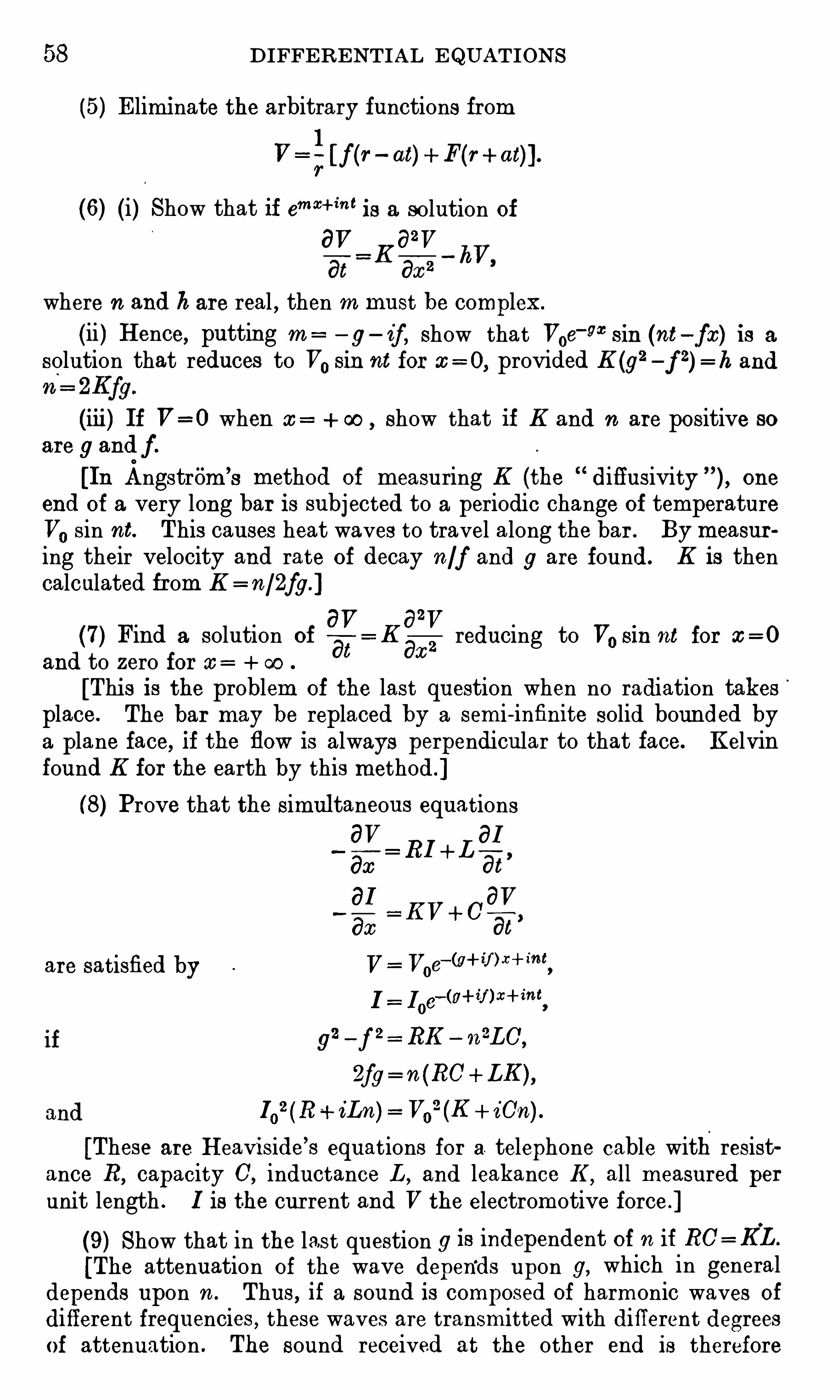
58 DIFFERENTIAL EQUATIONS
(5) Eliminate the arbitrary functions from
V= ; [f(r - at)
(6) (i) Show that if emaci‘i"t is a solution of
where n and k ar e real , then mmust be complex.
(ii ) Hence, putting m —g
— if , show that Voe‘ ” sin (nt—fz ) is a
solution that reduces to V0sin nt for z = 0, provided K(92 f 2) = h and
(iii ) If V= 0 when z = + 00 show that if K and n ar e positive soar e g and f .
[In Angstrom’
s method of measuring K (the diffusivity one
end Of a very long bar is subj ected to a periodic change Of temperatureV0 Sin nt. This causes heat waves to travel along the bar . By measur
ing their velocity and rate of decay n /f and g ar e found. K is thencalculated fr om K
2
(7) Find a solution ofS17
K0_ V reducing to V0sin nt for z =0at fiz z
and to zero for z 00
[This is the problem of the last question when no radiation takes '
place . The bar may be replaced by a semi - infinite solid bounded bya plane face , if the flow is always perpendicular to that face . K elvinfound K for the earth by this method ]
8) Prove that the simultaneous equations6V 81
amRI“
L bs?
81 aV
ar e satisfied by VI l
og
92 — f
2 RK n2LC',
2fg = n(RC + LK ) ,
1O2(R iLn) V0
2(K iC’
n) .
[These ar e Heaviside’
s equations for a telephone cable with resistance R,
capacity C,inductance L ,
and leakance K ,all measured per
unit length . Iis the current and V the e lectromotive force ]
(9) Show that in the last question 9 is independent of n if RC = K L[The attenuation of the wave depends upon 9, which in general
depends upon n . Thus, if a sound is composed of harmonic waves of
different frequencies, these waves ar e transmitted with different degreesof attenuation . The sound received at the other end is therefore

MISCELLANEOUS EXAMPLES 59
distorted . Heaviside’
s device of increasing L and K to make RC = K L
(10) In question if L = K = O, show that both V and I ar e
propagated with velocity[The velocity is given by n/f .]
(1 1) Show that the simultaneous equationst ap dy as
, ,u. da are ac ,
c at—
dy dz’
c dt dy dz’
k ao da dy . Mas aP aR,
c dt dz dz’
c dt dz dz’
11:dB dB da,u. dy dQ dB
0 dl dz dy c dt dz dy
ar e satisfied by P = O a = 0
Q= 0 ; B=Bo SinMOO— vi)
R= R0sin p (z — vt) ; y
= 0 ;
provided that and so= fl ak/MR,[These ar e
'
Maxwell ’s electromagnetic equations for a dielectric ofspecific inductive capacity It and permeability ,
u . P, Q,
R ar e the
components Of the electric intens ity and a , B, y those of the magneticintensity. 0 is the ratio of the electromagnetic to the electrostaticun its (whi ch is equal to the velocity of light in free ether) . The solutionshows that plane electromagnetic waves travel with the velocity c/X/FIL:and that the electric and magnetic intensities ar e perpendicular to thedirection of propagation and to each other .]
(12) Find a solution ofa
d—l/
= K g such that
V¢oo if t= 00 ;
V= 0 if z = 0 or W, for all values of t ;
V= 7rz z2 if t= 0, for values of z between 0and i r .
[N.B . Before attempting this question read again Arts . 46 and 49.
V is the temperatur e of a non - radiating r od of length 7r whose ends ar e
kept at the temperature of the r od being initially (7rz — z2)°at a
distance z from an end .]
(13) W hat does the solution of the last question become if thelength of the r od is l instead of 7r
[N.B . Proceed as in Ar t.
(14) Solve question (12) if the condition V= 0 for z = O or 7r is
replaced by g= 0 for z = 0 or 7r .
[Instead of the ends being at a constant temperature , they ar e heretreated so that no heat can pass through them .]
(15) Solve question (12) if the expression 7rz z2 is replaced by 100.

60 D IFFERENTIAL EQUATIONS
(16) Find a solution of such that
V# oo if t= co
V= IGO if z = 0 or 7r for all values of t ;V= O if t= 0 for all values of z between 0and W .
[Here the initially ice - cold r od has its ends in boiling water .](17) Solve question (15) if the length is l instead of 7r . If l fincr eases
indefinitely, Show that the infinite series becomes the integral200 1 _K a
,t— e sin az da .
[N .B . This is called a Fourier’
s Integral . To obtain this resultand 27r /l= da .
K elvin used an integral in his celebrated estimate of the age of the
earth from the Observed rate of increase of temperature underground.
(See example (107 ) of the miscellaneous set at the end of the book . )Strutt
’
s recent discovery that heat is continually. generated within theearth by radi o—active processes Shows that K elvin’
s estimate was toosmall ]
(18) Find a solution of K such that
V is finite when t= + 00 ;
7d_l= 0 when z = 0,
dz
V= O when.
z = l,
V= V0when t= 0, for all values Of z between 0and l.
[If a small test- tube containing a solution of salt is completelysubmerged in a very large vessel ful l Of water, the salt diffuses up out
of the test-tube into the water of the large vessel . If V0 is the initialconcentration of the salt and l the length of test- tube it fills, V givesthe concentration at any time at a height z above the bottom of the
test -tube . The condition d_V 0 when z = O means that no diffusiondz
takes place at the closed end. V= Owhen x= l means that at the topof the test- tube we have nearly pure water .]
azy 2d2y
(19) Find a solution of87
— 1) such that
y involves z trigonometric-allyy= 0 when z = 0 or 7r
,for all values of t ;
as
at
y= mz between z = 0 and
r all values of t
0when t= o, for all values of z
for all values Of l .71
y= m(7r — z ) between z =
§and 7
,

MISCELLANEOUS EXAMPLES 61
[N 48 .
y i ement of a string stretched between twopoints a d istance 7r apart . The string is plucked aside a distancem7r /2 at its middle point and then released ]
d2Writing the solution of D2
y, where D i s a constant,in
y=— e
xDA+ e‘ xDB
,
d_
2y_ d
2ydeduce the solution of in the form
dz_
2_
dl 2
— z )
by substituting da
tfor D
, f(t) and F(t) for A and B respectively ,and
using Taylor’
s theorem in its symbolical form
[The results obtained by these symbolical methods should be
regarded merely as probably correct . Unless they can be verified byother means , a very careful examination of the argument is necessaryto see if it can be taken backwards from the result to the differentia l
Heaviside has used symbolical methods to solve some otherwiseinsoluble problems . See his Electromagnetic Theory ]
drFrom the solution oi
dz2
that ofd_y
d y in the formdz dl 2 2 2 4
W f t + za— f +
z d f+
an 21 a“
= D2i where D is a constant , deduce
[This is not a solution unless the series is convergent ]Use this form to Obtain a solution which is rational , integral , and
algebraic of the second degree in t.d2y
a2d_
2
_y
dl2az
dz 2
pendent variables z and t to X and T, whereX= x - at ; T= z + at.
Hence solve the original equation .
Transform the equation by changing the inde
TO be omitted on a first r eading.

CHAPTER V
EQUATIONS OF THE FIRST ORDER BUT NOT OF THE
FIRST DEGREE
51 . In this chapter we shall deal with some special types of
equations of the first order and of degree higher than the first forwhi ch the solution can sometimes be obtained without the use of
infinite series .
These special types ar e(a) Those solvable for p.
(b) Those solvable for y.
(0) Those solvable for z .
52. Equations solvable for p. If we can solve for p,the equation
Of the n“L1 degree is reduced to n equations of the first degree , to
W hich we apply the methods Of Chap . II.
Ex . (i) . The equation p2 pz py zy 0 gives
P“ 27 01
'
P y ifrom which 2y
— z2+ c1 or z = — log y + oz ;
or, expressed as one equation ,
(2y+ z2
y
At this point we meet with a difficulty ; the complete primitiveapparently contains two arbitrary constants , whereas we expect onlyone, as the equation is Of the first order .
But consider the solution(2y + z
2y
If we ar e considering only one value Of each of the constants 0,cl ,
and 02,these equations each represent a pair of cur ves , and of course
not the same pair (unless But if we consider the infiniteset Of pairs of curves obtained by giving the constants all possiblevalues from 00 to 00 we shall get the same infinite set when takenaltogether, though possibly in a di fferent order . Thus (2) can be takenas the complete primitive .

EQUATIONS OF THE FIRST ORDER 63
p2+p
p= 1 or p= — 2
,
giving y= z + c1 or y=— 2z + cz.
As before , we take the complete primitive as
(y— z — c) = 0,
(y — z - c2) =0.
Each of these equations represents all lines parallel eithery=
. z or to y= — 2z .
p2+p W2) p
2+ 2zp = 3z
2. p
2= z5
.
(4) x+ yr2 =r (l (5) p
3
v (’
6) p2 — 2p cosh z + 1 = 0.
53 . Equations solvable for y . If the equation is solvable for y,we differentiate the solved form with respect to z .
Ex . (i) . p2
Solving for y, y=
dp 1 z dpDi fferentiating, _
da_
c+
p 192 dz
’
p17 dr 19
2
This is a linear equation of the first order , considering p as the
independent variable . Proceeding as in Ar t. 19, the student will Obtainz = p(c cosh
“ 1p)(p
2 1 )- 2
Hence , asP
These two equations for z and y in terms of p give the parametrice quations of the solution of the di fferential equation . For any given
p correspond one definite value of z and
As p varies, the point moves, tracing out
this example we can eliminate p and get the equation cony, but for tracing the curve the parametric forms ar e as
good ,if not better.
Ex . (ii) . 3p5 —py+ 1
= 0.
Solving for y, y 3194104
.
dr dz?Di fferenti ating, p 12193
do:p2
35,
dz (12p2p
—3)dp
Integrating, z 4113 $13
4 c,
and from above , y 3104194
.
The student should trace the graph of this some particular valueof c
,say c = 0.

64 DIFFERENTIAL EQUATIONS
54. Equations solvable for x. If the equation is solvable for z,
we differentiate the solved form with respect to y, and
in the form 1 .
P
Ex . p2 —py+ z =
— 0. This was solved in the last article byfor y.
Solving for z ,z = py
—p2
Differentiating with respect to y,l dp _
pP y
‘
dy
dri e = 2
p dp.
7/ P
which is a linear equation of the first order , considering p as the independent and y as the dependent variable . This may be solved as inAr t. 19. The student will obtain the result found in the last article .
Examples for solution.
(1 ) z = 4p + 4p3
.
(7) p3 —p (y+ 3) + z = 0.
(9) y= p tan p+ log cos p.
P(l l ) p — tan < l +p
2
(12) Prove that all curves of the family given by the solution of
Ex . 1 cut the axis of y at right angles . Find the value of c for thatcurve of the family that goes through the point (0,
Trace this curve on squared paper .(13) Trace the curve given by the solution of Ex . 9 with c =0.
Draw the tangents at the points given by p= 0, p = l , p = 2 and p= 3 ,
and verify , by measurement , that the gr adients of these tangents ar e
respectively 0, 1 , 2 and 3 .
(2) p2
M) y = w+ r 2
(6)
(8) y= p sin p + cos p.
(10) d" 2 =
p2 — 1 .
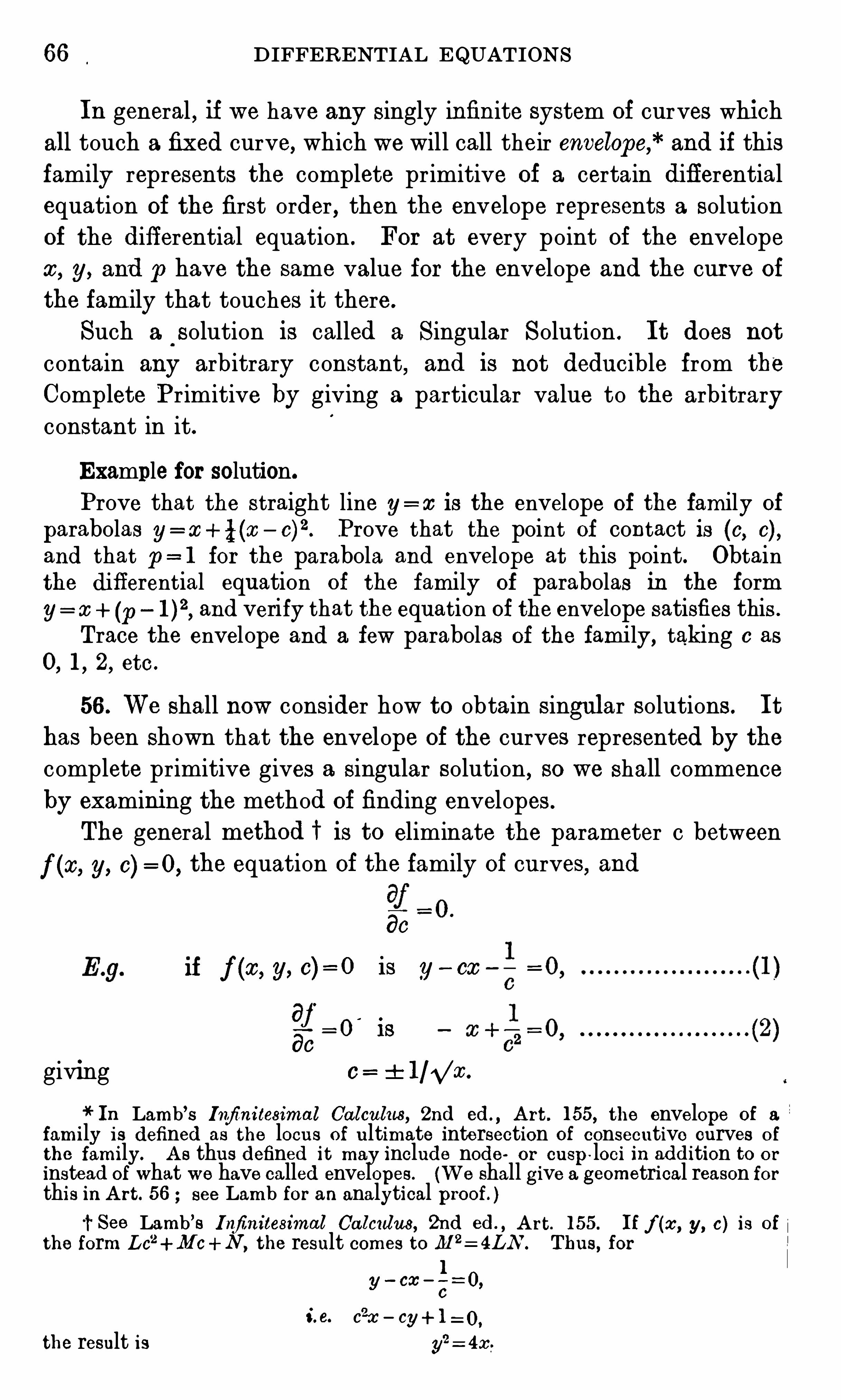
66 DIFFERENTIAL EQUATIONS
In general , if we have any singly infin ite system of curves whichall touch a fixed curve, which we will call the ir envelope,* and if thisfamily represents the complete primitive Of a certain differentialequation of the first order , then the envelope represents a solutionof the differential equation . For at every point of the envelopez , y, and p have the same value for the envelope and the cur ve of
the family that touches it there .
Such a solution is called a Singular Solution . It does not
contain any arbitrary constant, and is not deducible from the
Complete Primitive by giving a particular value to the arbitraryconstant in it.
Example for solution.
Prove that the straight line y= z is the envelope of the family of
parabolas y= z + i (z — c)2
. Prove that the point of contact is (c, c) ,and that p = 1 for the parabola and envelope at this point. Obtainthe differential equation of the family of parabolas in the formy z (p and verify that the equation of the envelope satisfies this .
Trace the envelope and a few parabolas of the fami ly , taking c as
0, 1 , 2, etc .
56 . W e shall now consider how to obtain singular solutions. It
has been shown that the envelope of the curves represented by thecomplete primitive gives a singular solution, so we shall commenceby examining the method of finding envelopes.
The general method l is to eliminate the parameter c between
f (z , y, 0) = 0, the equation of the family of curves, and
dc
if f (z , y, a) = o is y— cz
dj’
do0 i s
giving c = i l /Vz .
* In Lamb’s Infin itesima l Ca lculus, 2nd ed . , Ar t. 155, the enve lope of a
family is defined as the locus of ultimate inte rsection of consecutive curves of
the family . As thus defined it may include node or cusp-loci in addition to or
instead of what we have called envelopes. (W e shall give a geometrical reason forthis in Ar t. 56 see Lamb for an analytical proof . )’
l' See Lamb’
s Infinitesimal Ca lculus, 2nd ed . , Ar t. 155. If f (z , y, c) is Of
the form Lc2+M c+N ,the result comes to M 2= 4LN . Thus, for
ly
— cz —
ZO,
i. e. c2z cy + 1 =0,
the result is y2= 4z

SINGULAR SOLUTIONS 67
y2 4z .
Thismethod is equivalent to finding the locus of intersection of
f (x’ fl], 0) = 0,and f (z , y, c + li ) =0,two c urves of the family with parameters that differ by a smallquantity h, and proceeding to the limit when It approaches zero .
The result is called the c-discr iminant of f (z , y, c) = 0.
57 . Now consider the diagrams 8 , 9, 10, 1 1 .
Fig . 8 shows the case where the curves of the family havespecial singularity . The locus of the ultimate intersections
a cur ve which has two points in common with each-Of the cur ves of the family (e.g . Q and R lie on the locus and alsoon the cur ve marked In the limit the locus PQRSTUV therefore touches each curve of the family, and is what we have defined
In Fig . 9 each curve of the family has a node . Two con
secutive cur ves intersect in three points (e .g . curves 2 and 3 in thepoints P
, Q,and R) .
The locus of such points consists of three distinct parts EE'
,
AA’
, and BB'
.
When we proceed to the limit, taking the consecutive curvesever closer and closer , AA
'
and BB' will move up to coincidence
with the node - locus NN’
,while EE’ will become an envelope . So

68 DIFFERENTIAL EQUATIONS
in this case we expect the c-discriminant to contain the square o f
the equation of the node—locus, as well as the equation of the envelope .
E'r b flo wez
NZ 7 M ir
As Fig . 10 shows,the direction of the node - locus NN'
at any
point P on it is in general not the same as that of e ither branch ofthe curve with the node at P . The node- locus has z and y in commonwith the curve at P , but not p,
so the node- locus is not a solution of“
the difi'
er ential equation of the cur ves of thefamily.
FIG . 10.
If the node shrinks into a cusp , the loci EE’
and NN Of Fig . 10,
move up to coincidence , forming the cusp- locus CC’
of Fig . 1 1 .
Now NN was shown to be the coincidence Of the two loci AA’
and
BB'
of Fig . 9, so CC’
is really the coincidence of three loci , andits equation must be expected to occur cubed in the c—discriminant .Fig . 1 1 shows that the cusp- locus
,like the node - l ocus, is not
(in general ) a solution of the differential equation .
Fm. 1 1 .
To sum up,we may ezpect the c-discr iminant to contain
(i) the envelope, f fI
(ii) the node- locus squar ed,
(iii):the c usp- locus cubed.

SINGULAR SOLUTIONS 69
The envelope is a singular solution , but the node and cusploci ar e not (in general solutions at all.
58 . The fo llowing examples will illustrate the preceding resultsEx. (i) .The complete primitive is easily found to be 4y (z c)
i .e. c2 2cz + z 2 4y= O.
As this 18 a quadr atic in c, we can write down the discriminant atonce as 4(z
2 4g) ,
the envelope of the family of equal parabolasprimitive , and occurring to the fir st degree only,
FIG . 12.
3y 2pz 2
Proceeding as in the last chapter, we get
p2
— 4
2 2dp
t .e. pz- 2p
= (2z3
i .e . z2 2p= 0 or p
= 2z
dz d_p
z p
W e say in gener a l , because it is conce ivable that in some special example a
or cusp-locus may coincide with an enve lope or W i th a curve of the fami ly .

70 DIFFERENTIAL EQUATIONS
log z = 2 log p — log 0,
oz p2,
whence 3y 2cfz2 2c,
i .e . (3y a family of semi - cubical parabolas with their cuspson the axis Of y.
The c—discriminant is (3y z3)2 9y
2,
i .e. z3(6y z
3) = 0.
The cus'p-locus appears cubed, and the other factor represents theenvelope .
It is easily verified that 6y= z3 is a solution of the differential
equation , while z = 0(giving p= 00 is not .
If we take the first alternative of the equations (A) ,i .e. z
2 — 2p=0,
we get by substitution for p in the differential equation3y W ,
i .e . the envelope .
This illustrates another method of finding singular solutions.
Examples for solution.
Find the complete primitives and singular solutions (if any)following differential equations. Trace the graphs for Examples
(1 ) 4p2 — 9z = 0. (2) 4p
2(z
(3) zp2 (4) p
2 + y2
(5) p2+ 2zp
—y= 0. (6) zp
2
(7) 4zp2 4yp

SINGULAR SOLUTIONS 71
59. The p-discriminant. W e shall now consider how to Obtainthe singular solutions Of a differential equation directly from the
equation itself,without having to find the complete primitive .
Consider the equation z2p2yp 1 = 0.
If we give z and y any definite numerical values, we get a quad
r atic for p. For example , if
y = 3 , 2p2
p=
. Or 1 .
Thus there ar e two curves of the family satisfying this equationthrough every point . These two curves will have the same tangentat all poin ts where the equation has equal roots in p, i .e . wherethe discriminant y2 4z 2 0.
Similar conclusions hold for the quadratic Lp2 +Mp +N =0,
where L , M , N ar e any functions of z and y. There ar e two curvesthrough every point in the plane , but these cur ves have the samedirection at all p oints on the locus M 2 4LN = 0.
More generally , the differential equation
f (z , y, p) s Lopn+Ll p
n — 1 — 2+Ln
= O,
where the L’
s ar e fun ct ions Of z and y, gives n values of p for a
given pair of values of z and y, corresponding to n curves throughany point . Two of these n cur ves have the same tangent at allpoints on the locus given by eliminating p from
x, y, P) = O:
for this is the condition given in books on theory of equations forthe existence of a repeated root .W e ar e thus led to the p-discriminant , and we must now in
vestigate the properties of the loci represented by it .
60. TheEnvelope . The p-di scriminant of the equation
y = rw+lr
W e have already found that the complete primitive consists of
the tangents to the parabola ,which is the singular solution . Two
of these tangents pass through every point P in the plane, and
these tangents coincide for points on the envelope .

72 DIFFERENTIAL EQUATIONS
This is an example of the p—discr imin
Fig . 15 shows a more general case Of this.
FIG . 1 4.
Consider the curve SQP as moving up to coincidence with thecurve FRT
,always remaining in contact with the envelope QRU.
The point P will move up towards R, and the tangents to the twocurves through P will finally co incide with each other and with thetangent at the envelope at R. Thus R is a point for whi ch the pieof the two curves Of the system thr ough the point coincide , andconsequently the
‘
p-discriminant vanishes
FIG . 1 5 .
Thus the p-discriminant may be an envelope of the curves of
the system ,and if
'
so,as shown in Ar t. 55 , is a singular solution .
61 . The tac-locus. The envelope is thus the locus of pointswhere two consecutive curves of the family have the same valueof p. But it is quite possible for two non- consecutive curves totouch .
Consider a family of c ircles,all of equal radius
,whose centres
lie on a straight lin e .

74 DIFFERENTIAL EQUATIONS
of between two different curves,i .e . the p
-discr
a cusp .
As shown in Fig . 1 8, the direction Of the
point P on it is in general not the same as
the cusp , so the cusp- locus is not a solution of
FIG . 1 8 .
It is natural to enquire if the equation of the cusp - locus willappear cubed in the p-discriminant, as in the c-discriminant . Todecide this, consider the locus of points for which the two p
’
s are
nearly but not quite equal,when the cur ves have very flat nodes.
This will be the locusNN of Fig . 19. In the limit, when the nodesI
FIG . 19.
contract into cusps, we get the cusp - locus, and as in this case thereis no question of two or more loci coinciding , we expect the pdiscriminant to contain the equation Of the cusp - locus to the firstpower only .
64. Summary of results. The p-di scriminant therefore may be
expected to contain(i) the envelope,(ii) the tac- locus squared,
(iii) the cusp - locus,c-discriminant to contain
(i) the envelope,(ii) the node- locus squared,(iii) the cusp - locus cubed .

SINGULAR SOLUTIONS 75
Of these only the envelope is a solution differentialequation .
65. Examples.Ex. (i) . p
2(2 —y) .
Writing this in the formdz 2 3y
dyi2x/ (1 —
y)’
(w c)2=y2(1 y),
The c-discriminant and p-discriminant ar e respectivelyy2(1 y) = 0 and (2 - 3y)
2(1 y) =0.
1. y= O, whi ch occur s in both to the first degree, gives an envelopewhich Occurs squared in the c-discriminant and not at all in
the p-discriminant , gives a node - locus 2 3y
= 0, whi ch occur s squaredin ,
‘
the p-discriminant and not at all in the c-discriminant, gives a
It is easily verified that of these three loci only the equation Of the
envelope satisfies the differential equation .
FIG . 20.
Consider the family of circlesz2+ y
2+ 2gz + 2c2 1 = 0.
By eliminating c (by the methods of Chap . we obtain the di fferential equation
2y2p2 2zyp + z
2y2

76 DIFFERENTIAL EQUATIONS
The c and p-discriminants ar e respectively
z2 2(z 2 y
2 1 ) = 0 and z2y2 2y
2(z 2 + y
2 1 ) = 0,i .e. z
2+ 2y2
and y2(z 2+ 2y
2
z2 2y
2 2= 0 gives an envelope as it occurs to theboth discriminants, while y = 0 gives a tac- locus, as it occursin the p-discriminant and not at all
Examples for solution.
In the following examples find the complete primitive if the differential equation is given or the differential equation if the completeprimitive is given . Find the singular solutions (if any) . Trace thegraphs.
(1 ) 4z(z —l )(z — 2)p2 —(3z
2 (2) 4zp2 — (3z
(3) yp2 (4) 3zp
2
(5) p2+ 2pz
3 — 4z 2y 7= 0.
(6) p3
(7) z2+ y
2 (8) c2 + 2cy
(9) — zy= 0. (10) z 2 + y2 + 2ozy+ o
2 — 1 = O.
66. Clairaut’s Form.
* W e commenced this chapter by con
elder ing the equation ay = px “F
iAlexis Claude Cla iraut, Of Pa r is (1713 although best known in con
nection with d iffe r ential equations , wr ote chiefly on astronomy .

SINGULAR SOLUTIONS 77
This is .a particular case of Clairaut’
s Form
To solve, differentiate with respect to ps i .
10=P {w
dPthereforedz
0, p c,
(1 ) and (2) we get the complete primitive , the family of
(4)
If we e liminate p from (I) and (3 ) we shall simp ly get the p-dis
To.
fin d the c-discriminant we eliminate c fr om (4) and the result(4) partially with respect to c, i .e .
0 z fEquations (4) and (5) differ from (1 ) and (3 ) only in having c
instead Of p. The e liminants ar e therefore the same . Thus bothdiscriminants must represent the envelope .
_Of cour se it is obvious that a family of straight lines cannot
Equation (4) gives the important result that the complete pr imiForm may be wr itten down
wr iting 0 in place of p.
”
Find the curve such that 0T varies as tan tb , where T is the pointin which the tangen t at any point cuts the axis Of z , \/I‘ is its inclinationto. this axis, and 0 is the origin .
FIG . 22.

78 DIFFERENTIAL EQUATIONS
From the figure, 0T= 0N TN
z y cot x];
r,
P
tan T p
therefore 11 hp,
P
i .e . y=pz kp
2.
Thisis of Clairaut’
s Form, so the complete primitive is
y cz kc2,
and the singular solution is the di scrimi nant of this,i .e. z
2= 4ky.
The curve required is the parabola represented by thissolution . The complete primitive represents the family Of
lines tangent to this parabola .
Examples for solution.
Find the complete primitive and singular solutions of the followingdifferential equations. Trace the graphs for Examples (7
(8) and
W 1 ) y= pw+ r2 W2) y= rw+p3
v(3) y= pz + cos p. (4)
p= log (pz y) . (6) sin pz cos y= eos pz sin y+p.
(7 Find the differential equation of the cur ve such that the tangentmakes with the co-ordinate axes a triangle of constant area 102, andhence find the equation of the curve in integral form .
(8) Find the curve such that the tangent cuts Off intercepts fromthe axes whose sum is constant .
(9) Find the curve such that the part of the tangent interceptedbetween the axes is of constant length .
MISCELLANEOUS EXAMPLES ON CHAPTER VI.
Il lustrate the solutions by a graph whenever possible .
(1 ) Examine for singular solutions 192 2zp= 3z2.
(2) Reduce zyp2 — (z 2+ y
2
to Clairaut’
s form by the substitution X= z2 Y =
y2
.
Hence Show that the equation represents a family of conics touchingthe four sides of a square .

MISCELLANEOUS EXAMPLES 79
of confocal conics, with the foci at (i h ,touching
lines joining the foci to the circular points at infinity .
(4) Show by geometrical reasoning or otherwise that the sub
z = aX + bY,
Converts any differential equation of Clairaut’
s form to another equationof Clairaut’
s fo
(5) Show that the complete primitive of 8p3z = y(l 2p
2 9) is
(x+ c)3 = 3y
2c, the p
-discriminant y2(9z
2 4y2) = 0, and the c-dis
cr iminant y4(9z
2 4y2) = 0. Interpret these discriminants.
(6) Reduce the di fferential equation
z2p2yp(2z y) y
2= 0, where p
to Clairaut’
s form by the substitution f = y, 7; zy.
Hence , or otherwise , solve the equation .
Prove that y+ 4z = 0 is a singular solution and that y=0 is bothpart of the envelope and part of an ordinary solution . [London ]
2
(7 Solve y2(y zg—Z)= z
4 which can be transformed to
Clairaut’
s form by suitable substitutions . [London ](8) Integrate the differential equations
(i) - <v)3
(ii) y2(1 4p2) 2pzy
— 1 = O.
In (11 ) find the singular solution and explain the significance of anyfactors that occur . [London ]
(9) Show that the curves of the familyy2 — 2cz 2y+ c
2(z4 — z
3) =0
all have a cusp at the origin , touchi ng the axis of z .
By eliminating c obtain the differential equation of the family inthe form
4p2z2(z 1 ) — 4pzy (4z — 3y) + (16z 9)y
2=0.
Show that both discriminants take the form z3y2 = 0, but that z =0
is not a solution, while y Ois a particular integral as well as an envelope .
[This example shows that our theory does not apply without modification to families of curves with a cusp at a fixed point ]
(10) Show that the complete primitive Of
represents the family of equal lemniscates of Bernoullir2
a2cos a ) ,
inscribed in the circle r = a ,which is the singular solution , with the
point r = 0as a node—locus .

80 D IFFERENTIAL EQUATIONS
(1 1 ) Obtain and interpret the complete primitivesolution of
dr 2
dd) + r 2 — 2r a = 0.
(12) Show that r 06 02 is the complete primitive and 4r = 92 the
gular solution ofdr dr 2
dd dd
Verify that the singular solution touches the completethe point (c2, the common tangent there making an angle tan - l
o
with the radius vector.

82 D IFFERENTIAL EQUATIONS
W e shall use suffixes to denote differentiations with respect todza
z , e.g . y2 for dx2’ but when the independent variable is any other
than z the differential coefficients will be written in full .
69. y absent. If y does not occur explicitly in an equation of
the second order , write p for y1 and for yz.
W e obtain an equation containing only p, and z , and so
the first order . 0
Consider, for example, xyz + y1 4z .
This transforms into zd_p
p
which can be integrated at oncezp 2z 2 a ,
at .e . p
= 2z +x
By integrating, y= z
2a log z b,
Evher e a and b ar e arbitrary constants.
This method may be used to reduce an equation of the nth order’
not containing y explicitly to one of the (n
70. x absent. If z is the absent letter, we may still write 19 for
y,, but for y2 we now write q sincedp dp The
dy’
dy dd= y2'
procedure reduces an equation of the second order without z to one
of the fir st order in the variables p and y.
For example , yy2 = y12
transforms into p2,
from which the student will easily obtainp= by and y
= aeb”
.
Examples for solution.
A ccez z = l . (2) yyz+ y12=y1 l (3) yy2+ 1 = y1
2.
(4) Reduce to the previous example , and hence solveai r s + y1
2= 2yz2
(5) Pys+ y2= 1223 (6) ga ‘ zyn - i
(7) Integrate andinterpret geometrically(1 M

EQUATIONS OF SECOND AND H IGHER ORDERS 83
(8) .,The radius of curvature of a certain curve is equal to the length
of the normal between the curve and the axis of z . Prove that thecording as it is convex or concave to
(9) Find and solve the difier ential equation of the curve the lengthof whose ar e, measured from a fixed point A to a variable point P, is
proportional to the tangent of the angle between the tangent at P and
the axis of z .
71 . Homogeneous equations. If z and y ar e regarded as of
dimens ion 1 ,yl is of dimension 0,
y2 is of dimens ion 1 ,
31 3 is of dimension — 2,
define a'
homogeneous equation as one in which all the termsthe same dimensions. W e have already in Chap . II. dealt
of the first order and degree, and inlinear equation
zfl
yn Az n‘ lynq Bz ” Hzy1 K y =0
(where A, B , H, K ar e merely constants) , for which we used thesubstitution z = e‘
or t= log z .
Let us make the same substitution in the homogeneous equationwan 3n
dl dy l dyyl = dz dl z dl
’
dy1 1 dy+1 d dy
W z2 dt
+z dz dt
1 dy+1 dt d2y
z2 dt
+z dz dt2
1 dy+l d2y
.
z2 dl
+z2 dl2
(1 ) and multiplying by z ,we get
ri ff-t? 33+ w il
l—l
i e' 237? (dt>This is an equation , with t absent, similar to those in the last
absent .
Arts . 71 -73 may be omitted on a first reading .

84 D IFFERENTIAL EQUATIONS
By putting q, the student will easily obtain
w= 2 (y2
giving t c log (y2
Hence y2 b= cw“ )
az“, replacing c“ by another arbitrary constant a .
72. The example of Art . 71 came out easily because it hadsuperfluous z ’
s left after associating z 2 with y2 and z with yl .fact, it could have been written
3; ($tBut
cannot be so wr itten . To reduce this to a form similar to thatthe last example , put y = vz , a substitution usedequations in Chap . II.
(2) becomes(z2
zzvz)(vz vl z
2Oz ) z
4112(zv2 2111) 0,
i .e. (1 + fv2)v1 -1 + 2111 ) = O,
which may be wr itten 02x202= (1
W e now proceed as before and put z = e‘, giving
dv(1701
(
“
l—
t
2(PO do
“5 ”2 dt2 dt‘
d2 d do
(3) becomes “(d— ti.)
if) : — v2) df
a
2d% do
we . vz
dtz di
an equation wi th t absent.dv dz?) (13As before , put dt
= q.(F
(4) becomes vzqii
i—g= q.
Ell
—Z: ”
12 (un less q= 0, giving y
(E _1_ 1
di— q
a v’
cwdo a2
diOw (“HT— 71
do,
t= av+ a2 log (1) —a) + b,
and finally log z ay/z (12 log (y az ) a
2 log z b.

86 DIFFERENTIAL EQUATIONS
dl 1
dz p V(a — z
1 zt= s1n
“ 1+ const . ,
p a
z = a sin (pt
Hence
Examples for solution.
(1 ) y2= y3 —y, given that y1 = 0 when y= 1 .
(2) y2= e2y
, given that y= 0 and yl = l when z = O.
(3) y2= sec2y tan y, given that y=0 and y1 = 1 when z =0.
dzz ga2 dz
(4) given that z = h and when t= 0
[h z is the distance fallen from rest under gravity varying inverselyas the square of the distance z from the centre of the earth, neglectingair resistance , etc .]
dzu P(5)
61—
62+ u
hzuz’ in the two cases
i P = ,uu2 ; (11 P = u
"(l u
given that when u 2, where ,u , h, and c ar e constants.
[These give the path described by a particle attracted to a fixed
point with a force varying inversely as the square and cube respectivelyof the distance r
.u is the reciprocal of r , 9 has its ordinary meaning
in polar co-ordi nates, M is the acceleration at unit distance, and h istwice the areal velocity ]
X 75. Factor isation of the operator . The lin ear equation(z + 2)y2 (2z + 5 )yl + 2y (z l )e
“’
may be written as
{(z + 2)D2(2z + 5)D + 2}y = (z
where D stands for£0, as in Chapter III.
Now the operator in this particular example can begiving - l }(D
Put (D 2)yThenTh is is a linear equation of the first order . Solving as
W 3 get
t.e. (D 2)y = c(x + 2)
another linear equation , giving finallyy a(2z 5) be? ”
e”, replacing 10 by a .

EQUATIONS OF SECOND AND HIGHER ORDERS 87
Of cour se it is only in special cases that the operator can befactorised. It is important to notice that these factors must bewr itten in the right order , as they ar e not commutative . Thus, onreversin g the order in this example , we get
(1) + 2)D 1 }y {(z + 2)D2 - (2z + 4)D + 2}y.
(1 ) (2) zy2+ (z — l )y1 —y=0.
(3) zy2+ (z — l )yl -
y= z
2.
given that y= 2 and y1=0 when
(5) (z 2 l )yz (4x2 3z 5)y1 + (4z2 6z given that y= 1
and y1 2 when z =0.
76. One integr al belonging to the complementary function known .
When one integral of the equation
is known , say y = z, then the more general equation of the second
yz +Py1 +Qy = R, (2)
wher e'
P, Q, R ar e functions of z , can be reduced to on e of the fir st
order by the substitution y= vz.
Differentiating, y1 el z vzl ,
y2fuzz 20121 vzz.
Hence (2) becomesO22 vl (2z1 Pz) 1) (z2 l Qz) = O,
i .e. z
S ince by hypothesis
(3) is a linear equation of the first Order in 01 .
Similarly a linear equation of the nth order can be reduced to
one
'
of the (n — 1 )th if one integral belonging to the complementary
function is known .
77 . Example.
Consider again the equation
(z + 2)y2
The proof of Ar t. 29 that the gener al solution of a linea r d ifi'
er entia l equation is
the sum of a Par ticular Integr a l and the Comp lementar y Function holds good whencoefficients ar e functions of z as well as in the case when they ar e constants.

88 DIFFERENTIAL EQUATIONS
If we notice that y= e2‘” makes the left -hand side of the equation
zero , we can put y= ve2”
,
yr= (v1
y2 (v2 M ) e“
.
Substitution in (4) gives(2z + 5)} vl e
zx
d
Solving this in the usual way (by finding the integrating factor )we Obtam ”1
= e— 2z
Integrating, v e“
} C(2z 5) e‘ u b,
whence y= ve2x=
Examples for solution.
(1 ) Show that y2+ Py1 + Qy=O is satisfied by y= e” if 1
and by y= z if P +Qz = O.
(2) x2y2+ xy1
-
y= 8w3
(3) z 2y2 (z2 2z )y1 (z 2)y z
3ea’
.
(4) zy2 - 2 y= (z
(5) z2y2+ zy1 9y
= 0, given that y = z3 is a solution .
(6) zy2(z cos z — 2 sin z ) (z 2 4- 2)y1 sin z — 2y (z sin z + cos z ) = O,
given that y= z2 is .a solution .
78. Var iation of Parameters. W e shall now explain an elegantbut somewhat artificial method for finding the complete primitiveof a linear equation whose complementary function is known .
Let us illustrate the method by applying it to the examplealready solved in two different ways, namely ,
(z + 2)y2 (2z + 5 )y1 + 2y = (z 1 )
of whi ch the complementary function is y a(2z 5 ) be“.
Assume that y (2z 5 )A es ,
where A and B ar e fun ctions of z .
This assumption is similar to , but more symmetrical than, thatOf Art. 77 , VIZ .
y = v62z
’
Differentiating
y1 = (2z + 5)AI+ 62“°B l + 2A + 262xB . (3 )
Now so far the two functions (or parameters) A and B are onlyconnected by the single equation W e can make them satisfythe additional equation
(2z 5)AI as ,=0.

90 DIFFERENTIAL EQUATIONS
A B RSolving (4) and 7
0
3
T ; W 1— uv1
W e then get A and B by integration, sayA =f (x) M .
B = F (z ) + b,where f (z ) and F (z ) ar e kn own functions of z , and a and b are
a rbitrary constants.
Substituting in we get finally= uf (z ) + vF (z ) an be .
80. This method can be extended to linear equations of anyo rder . For that of the third order,
of which the complementary function y =— au + bv + cw
m
is supposedknown , the student will easily obtain the equations
provided thathence y2 uzA vZB wzC,
provided that 0 ulAl 013 1 W101
y3 usA v3B + 1030
11 2A1 czB1 10201
by substitution in (l S 0. l 1”23 1 + 1s ,
AI, B1 , and 01 ar e then found from the three equations (6)and
Examples for solution.
(1 ) y2+ y= cosec z . (2) y2+ 4y= 4 tan 2z .
2(3) y2 “
y1 + e
x.
(4) zzy2 zy1 y given the complementary function az bz
—l.
(5) ya Ggg Hy] 69= ezx
o
81 . Compar ison of the different methods for solving linear equations.
If it is required to solve a linear equation of the second order andn o special method is indicated, it is generally best to try to guessa particular integral belonging to the complementary function andproceed as in Art . 76. This method may be used to reduce a lineare quation Of the n'“h order to one of the (n
To be omitted on a first reading.

EQUATIONS OF SECOND AND HIGHER ORDERS 91
The method of factorisation of the operator gives a neat solutionin a few cases, but these ar e usually examples specially constructedfor this purpose . In general the operator cannot be factorised.
The method of variation of parameters is inferior in practicalvalue to. that of Ar t. 76, as it requires a complete knowledge of the
c omplementary function instead of only one part of it. Moreover ,if applied to equations of the
.
third or higher order,it requires too
much labour to solve the simultaneous equations for AI, B1 , 01 , etc . ,
and to perform the integrations.
MISCELLANEOUS EXAMPLES ON CHAPTER VII.
(1 ) (2) zy2+ zy12 -
y1 =0.
(3) 4z.- 1. (4) yu_z 8 cos 3z .
(5) 73 x2)yz $91 9
= 0'
(6) (z2 2z l )yz (3z
2 8z l )y1 (2z 2
(7 Verify that cos nz and sin nz ar e integrating factors ofy2 n
zy (z ) .
Hence obtain two first integrals ofy2 n
zy sec nz ,
and by elimination of y1 deduce the complete primitive .
(8) Show that the linear equationAy+ By1 + + Syn = T,
where A,B
, C,T ar e functions of z ,
is ezact, i .e . derivable immediately by difier entiation from an equation of the next lower order , ifthe successive difier ential coefficients of A,
B,C,
satisfy the relationA B
1 + Cz
[N .B .— By successive integration by parts,
Syndz = Syn- 1 7 Slyn—2“l' Sayn—s l " dz .]
Verify that this condition is satisfied by the following equation , andhence Solve it
(9) Verify that the following non - l inear equations ar e exact, andsolve them (i ) W 2 + y1
2= 0.
(11) yyl O
(10) Show that the substitution y= ve
" %lp d“
y2'
+ Pyl +Qy R.
where P, Q,and R ar e functions of z , into the Normal Form
cz+ l v
= S ,
transforms

92 DIFFERENTIAL EQUATIONS
where I= Q ' iP 1 — iP2,
and S Rei lp dx
Put into its Normal Form,and hence solve
y2 4zy1- 1 )y 36 97
2
sin 2z .
(1 1) Show that if the two equationsye Pyl = 0
and zz+pzl + gz
= 0
reduce to the same Normal Form,they may be transformed
each other by the relation
yel l-
P dz
zeflp dx
i.e. the condition of equivalence is that the Invar iant I should be thesame .
(12) Show that the equationsz2y2
-1-2(z3 - z )y1 — 2z 2)y= 0
and — 2z 2) z = 0
have the same invariant , andfind therelation that transforms one intothe other . Verify by actually Carrying out this transformation .
(13) If u and su ar e any two solutions ofv2+ Iv= O,
prove that 2 : 2u1
8 1 u2
and hence that8 3 3
(22>s
12 3
1
From (2) show that if s is any solution of sl
—éand 33
,
- lf
solutions of[The function of the difier ential coefficients Of
‘
s on the left-handSide of (3) is called the Schwarzian Der ivative (after H. A. Schwarz of
Berlin) and written { 3 , z } . It is Of importance in the theory of the
Hypergeometric Series }(14) Calculate the Invariant Iof the equation
z2y2
Taking s as the quotient of the two solutions z e”and z
, verify that{ s, z } 21
,
and that 3 1 i and 33 1
—5ar e solutions of the Normal Form of the original
equation .
(15 ) If u and v ar e two solutions of
prove that vu2 P(av1 vul ) 0,
and hence that fav1
vu 1 as
- lp dx.
Verify this for the equation of the last example .

CHAPTER VIII
NUMERICAL APPROXIMATIONS TO THE SOLUTION OF
DIFFERENTIAL EQUATIONS
82. The student will have noticed that the methods given in thepreceding chapters for Obtaining solutions in finite form only applyto certain Special types of difier ential equations. If an equationdoes not belong to one of these special types, we have to use approximate methods. The graphical method of Dr . Brodetsky, given inChapter I. , gives a good general idea of the nature of the solution ,but it cannot be relied upon for numerical values .
In this chapter we shall first give Picard’
s method for gettingsuccessive algebraic approximations. By putting numbers in these ,we generally get excellent numerical resul ts. Unf ortunately the
method can only be applied to a limited class of equations, in whichthe successive integrations can be easily performed .
The second method, which is entirely numerical and of muchmore general application, is due to Rungesl With proper pr ecautions it gives good resul ts in most cases, although occasionallyit may involve a very large amount of arithmetical calculation . W e
shall treat several examples by both methods to enable their meritsto be compared.
Variations of Runge ’
s method have been given by Heun , K utta,and the present writer .
83. Picard’s method of integrating successive approximations. The
differential equation d
if f (90 y)E . Picard, Professor at the University of Paris, is one of the most distinguished
mathematicians Of to day. He 18 well known for his rese arches on the Theory of
E motions , and his Cour s d’
analyse is a standard text book .
+0. Bun
gle ,
dBProfessor at the University of Gottingen, is an author ity on
graphical met

NUMERICAL APPROXIMATIONS
where y = b when z = a, can be wr itten
y= b f (z , y) dz .
For a first approximation we replace"
the y in f (z , y) by ba second we replace it by the fir st approximation , for a third bysecond, and so on .
Ex . (i) . z + y2, where y= 0 when z = 0.
y= (z + y2) dz .
First approz imation . Put y= 0 in z + y2,giving
z dz = §z 2
Second approz imation . Put y W in z + y2, giving
y (z lf z“)dz é—z
zglvz5
Third approz imation . Put y £z 2 fi z5 in z y
2, giving
y (z i—z“
71
3 1107
I il
mzw) dz
%_x2
916 f 1
1$8 1
x11,
and so on indefinitely .
Ex.
where y= 1 and z = l» when z = O.
Here y= 1 + z dz and
Fir st appr oz imation .
y= 1 + % dz = l + -lg z ,
z= g+ -g-x4
.
Second appr oz imation .
y= 1 + dz = 1
95

«96 DIFFERENTIAL EQUATIONS
Third approz imation .
y l gz"
-
1
1
3 z5
Bif zs) dz
1 -%z + 316 z6
T é—zzg,
-z4 + 1
7
7 n +£Iz 8) dz
x9+ s i7 r90
1 2,
a nd so on .
zy
x . (iii) 332 x3(Z—Z ' l' y ,) where y= l and El
l—Z : when z = 0.
By putting31 z, we reduce thi s to Ex .
It may be remarked that Picard’
s method converts the diff erentiale quation into an equation involving integrals, which is called an IntegralEquation .
Examples for solution.
Find the third approximation in the following cases. For examples(1 ) and (2) obtain also the exact solution by the usual methods .
x/ (l ) dz= 2y 2z 2 3 , where y= 2 when z =0.
i sN (2) {if
where y— 2 when z 1
dy
a;2$ + Z ,
dz2
61—
233zy+ z 2,
where y 2 and z 0 when z 0
CL?!dz
2
dzz e + z
4y,
where y=— 5 and z = 1 when z = O.
(5)d—z
—y weir/ + 2. where = 5 andd—y 1 when z =
— o.
(17 2xdz
y’ y: dz
84. Determination of numer ical values from theseSuppose that in Ex. (i) of the last article we desir e the value of y,
correct to seven places of decimals, when z =0-3 .
Substituting z =O°3 , we get 510 =O~045 from the fir st approxi
mation .
The second adds 71
c (0’3)
5
while the third adds =O~OOOOOO41

98 DIFFERENTIAL EQUATIONS
the y =NQ of any other point on the same characteristic , given thatz = 0N = a + h, say . A first approximation is given by taking thetangent PR instead of the characteristic PQ, i .e . taking
y =NL +LR=NL +PL tan LRPL = b+ hf (a, b) = b+ hf0, say .
But unless h is very small indeed, the error RQ is far fromnegligible .
A more reasonable approximation is to take the chord PQ as
parallel to the tangent to the characteristic through S , the middlepoint of PR.
Since fgis (a +%h, b this gives
y =NL +LQ=NL +PL tan LQPL = b + hf (a + i i , b
This simple formula gives good results in some cases, as will beseen fr om the following examples
given that y=0 when z =0, requi red y when
a = b=o, h=0°3 ,
fo=f (a, b) = 0, b+2hf0= 0,
giving > <f (0-15 ,
The value found in Ar t. 84 was so the error isabout per cent .
Ex. 33 —g; given that y= 2 when z = l , find y when z = l -2.
Here a = l , b= 2, h=0°2, f0= 2
Therefore xf (1 ° l , 2)
2
)2+02 x(2 -
fi
Now the differential equation is easily integr able, giving y= z +
so when z = 1 °2 the value of y is 2 033 The error isis rather large compared with the increment Of y, namely 0
Ex. (iii) . 35 f (x. y.a say.
if; y, z). say ;
given that y= 1 and z = 0~5 when z =0, find y and 7. when z =0°5.
Here a =o, b= 1 , c(the initial value of h= 0°5 .
Hence fo=f (0, l , -5 ; go= g(0, l ,

NUMERICAL APPROXIMATIONS 99
By an obvious extens ion of the method for two variables , we takehf (a + §h, b+ ihfi , c + %hg0) 1 +05 xf (0-25 ,
c + §hgo)xg(0°25, 1
-125 , 05 ) =C°5l 27 .
The accurate values, found as in Ar t. 84, ar e
y= 1 and z =0
Thus we have Obtained a fairly good result for y, but a very bad
about the degree of accur acy of the result deprives;he method of most of its value . However, it forms an introduction tohe more elaborate method of Runge , to be explained in the next1'
rticle .
Examples for solution.
(1 ) (z2y)*1 given that y= 4 when z obtain the value
-122 when z = 2-7 . [Runge’
s method gives
(2) =
1
1—
o{yi 1 + log,(z given that y 2when z I, obtain
;he value y= 2°194 when z = l . [Runge’
s method gives
ZZ= 2z 2; given that y 2when z = I, obtain the value y== 2 O76
z = 1 2. Also show that y=§z 2+ so that when z =- l 2, y is
ly 2
86. Runge’s method. Suppose that the function of y defined by
(z , y) , y= b when z = a,
denoted by y = F(z ) .If this can be expanded by Taylor
’
s theorem ,
F(a h) = F(a) hF’
(a)kg
IF
”
(a) +3
ks
!F (a) +
Now F'
(w) Z—Z =f (x. y) =f , sayW e shall now take the total difier ential coefficient with respectz (that is, taking the y in f to vary in consequence of the variationz ). Let us denote par tial difier ential coefficients by
azf azf ajr .
az’
a’
y ae r az ay’
ay2
their values when z = a and y = b by po, go, etc .
The conditions under which the difie rential equation and the initial condo defin e a function ar e discussed in Chap. X . The graphical treatast article assumes that these conditions are satisfied .

100 DIFFERENTIAL EQUATIONS
dr
(To:a dy aSimrlar ly, F (z ) (55; a? )(p +fq)
r +pg +fs +f (s + g2+ft).
ThusF(a h) F(a)
kfc Wm) +fogo) 2foso+fozio+P090+f070
2) (1 )
The first term represents the first approximation mentioned andrej ected in Art . 85 .
The second approximation of Ar t. 85, i .s.
y— b = 7&f (aHeb, b+ %kfo) = k1 , say.
may now be expanded and compared withNow, by Taylor
’
s theorem for two independent variables,may.»
1=fo ihpo i ii/
£
070 Q (Iihzl'o 2727030 317170
250)
giving k, hjo l imp, +f0qo) —g,-k3(ro 2f0s0+20)
It is obvious that k1is at fault in the coefi‘icient of h3 .
Our next step is suggested by the usual methods for the
numerical integration of the simpler differential equationdy(E:
—f (95
Our second approximation in this case reduces to the TrapezoidalRule
y
Now the next approximation discussed is generally Simpson’
s
Rule , which may be written
y
If we expand the corresponding formula in two variables, namelyt’dfo+ 4f (a +541. b+ %hfo) +f (a + b, 6
we easily obtainhf0+ %h
2(po+f0qo)
whi ch is a better approximation than kl , but even now has not the
coefficient of h3 quite in agreement withTo obtain the extra terms in h3 , Bunge ]
L replaceshf (a + h, b + t )
See the text- books on Calculus by Gibson or Lamb .
TMathematische Annalen , Vol. XLVI. pp. 167-178.

102 DIFFERENTIAL EQUATIONS
than this difference 0-0004. That is to say, we conclude that the valueis 0045 , correct to the third place Of decimals.
W e can test this conclusion by comparing the result obtained inAr t . 84, viz .
Ex.
- 90
; given that y= 1 when z = 0, find y when z = l .
This is an example given in Runge’
s original paper . Divide therange into three parts, 0 to 0-2
, to 05 ,05 to 1 . W e take a smallincrement for the fir st step because f (z , y) is largest at the beginning.
First step. a = o, b= l , h= 0°2,
0200 ;
k -2 xf (0'2,1 -2) = 0-143 ;
b+ k ) = O°2 xf (O-2, 1
-3 xf (0'1 , 1-1 )
> <O~34O 0-1 70 ;
giving y= 1 -168 when z = 0~2.
Second step.
a = o-2, b= 1 ~168, h= 0'3 ,
Proceeding as before we get k1 = O-17O, h2= 0'173 and SO k= 0°l 7l ,
giving when z = 0°5 .
Third step. a = 0°5 , b= 1 ~339, h= O-5 .
W e find giving y= 1 -499 when z = l .
Considering the k and kl , the error in this result should be less than0001 on each of the first and second steps and negligible (to 3 decimalplaces) on the third, that is, less than 0002 altogether.As a matter of fact , the true value of y is between 1 -498 and 1 4 99,
so the err or is less than 0001 . This value of y is found by integratingthe equation , leading to
71 2 tan loge(z
2y2) .
Examples for solution.
Give numerical results to the following examples to as many placesof decimals as ar e likely to be accurate
(1) ZZ
Z—i= l—
l
diyi
“ 1 given that y= 2 when z =
y when z = l , taking h= 2 (as f is very small ) .(2) Obtain a closer approximation to the preceding question
taking two steps.
(3) dz (z2—y)2— l ; given that y= 4 when z = 2~3
,find y
z = 2°7 (a) in one step, (b) in two steps.

NUMERICAL APPROXIMATIONS 103
l(4) Show that if —2and y= 2 when z = 1 , then y=— z +
Hence find the err ors in the result given by Runge’
s method, taking(a) h (b) h= O'2, (c) h= O°I(a single step in each case) , and comparethese errors with their estimated upper limits .
(5) If E(h) is the error of the resul t of solving a difier ential equationof the fir st order by Runge
’
s method, prove thatE(h) 1
a
I—
‘
foE(7272)=
724
Hence show that the error in a two-step solution should be aboutof that given by one step ; that is to say, we get the answer correct
to an extra place of decimals (roughly) by doubling the number of steps.
88. Extension to simultaneous eqiiations. The method is easilyextended to simul taneous equations. As the proof is very similarto the work in Ar t. 86, though rather lengthy, we shall merely givean example . This example and those given for solution ar e taken,with slight modifications, from Runge
’
s paper .dv
EX.
dz27. —g f (z y, z) , say,
dz yg lx, z) , Say ;
given that y= o'2o27 and z = 1 0202 when z = 0°2,
find y and z whenz = 0°4.
Il erea = o-2, b= o°2027, c = 1 0202, f0— f 02,
h= 02 ;
= hf0=0-2 x 1027 0-2054
l’= hgo= 0
-2 x02070 00414
k = hf (a -+h, b+ k'
,xf (0'4
, 04081 , 1 0616) 02206 ;
l b+ k'
-2 xg(0-4, 04081 , 1 0616) 00894 ;
b+ k -2 xf (0‘4,
=0-2322 ;
b+ k"
,x g(O
-4,04 233, 1
-1096) =0-O934 ;
b+ yc'
,xf (o
-3, 03054, 10409) = O-2128
l1'= hf xg(0
°3, 00054, 1 0409) = O-0641
02027, 10202) = l 027,
k2-0-2188
l,= l (l
’
00674
k= k + ~
g (hz — kl ) = o 0-2148 ;
— l1 ) =00641 +0
-001 1 00652 ;
giving y= 0-2027 +0-2148 =0-41 75
and z 1 0202 00652 1 0854,
probably correct to the thi rd place of decimals .
* The rest of this chapter may be omitted on a first reading.

104 D IFFERENTIAL EQUATIONS
Examples for solution.
(1 ) W ith the equation of Art . 88, show that if y=0-4175 andz 1 0854 when z = 0~4
,then y= 0-6614 and z = 1 2 145 (probably correct
to the thi rd place of decimals) when z = 0~6.
r aha given that w= 0°7500
and when z = 1 ~2145 , obtain the values m= o-5163 and r = 0'7348
when z (which is to be taken as the independentShow that the value of 7 1s probably correct to four decimal places , butthat the third place in the value of tomay be in error .(3) By putting w= oos 95 in the last example and y= sin gb, z = r in
the example of Ar t. 88, obtain in each case the equationsdz sin 95
677:tan 96 22T
which give the form of a drop of water resting on a horizontal plane .
89. Methods * of Heun and K utta. These methods ar e verysimilar to those of Run ge , so we shall state them very briefly . The
dy) and y == b when z = a, to find
+ cos gbd
d¢,
problem is:given that
the increment k of y when the increment of z is h.
Heun calculates successively= hf (a, b),
k"= hf (a + %h, b
k’"
= hf (a + %h, b +gand then takes i-(k
’
+ 370 as the approximate value of k.
K utta calculates successively,
= hf (a, b),k"= kf (a —h, b
k’"
= hf (a + §h, b + k”
k” ”
= hf (a + h, b + k k"
and then takes (k'
+ 379 3k’"
as the approximate valueof k.
The approximations can be verified by expansion in a Taylor’
s
series, as in Runge’
s case .
Example for solution.
G iven thatd—y=u and y= l when z =0, find the value of y (to 8dz y+ z
significant figures) when z = l -2 by the methods of Runge , Heun ,and
K utta and compare them with the accur ate value 1 1 678417 . [FromK utta s paper . ]
Z eiwchr iftfur Mathematz'
lc and Physik, Vols . 45 and 46.

106 DIFFERENTIAL EQUATIONS
As an approximation to the value of the integral it is best tot ake , not the arithmetic mean of A and B , but §B which isexact when PQR is an ar c of a parabola with its axis parallel to theaxis of z . It is also exact for the more general case when
as is proved in most treatises on the Calculus in their discussion of
Simpson’
s Rul e .
92. Extension of preceding results to functions defined by differentiale quations. Consider the function defined by
dy _
Ei" f(x’ y), y — b when z — a
,
where f(z , y) is subj ect to the following limitations in the range of
values a to a + h for z and b— h to b + h for y. It will be seen fr omwhat follows below that the increment of y is numerically less than h,so that all values of y will fall in the above range . The limitationsar e
(1 ) f(z , y) is finite and continuous, as ar e also its fir st and secondpartial difier ential coefficients.
(2) It never numerically exceeds unity . If this condi tion is notsatisfied, we can generally get a new equation in which it is satisfied
by taking y instead of z as the independent variable .
(3) Neither clf’y/dz3 nor af/ay changes sign .
Let m and M be any two numbers, such that1 2 m f M E 1 .
Then if the values of y when z is a + %h and a + h ar e denoted byb +jand b + 70 respectively ,
*
(1 )and — hf mh< k < Mh i h. (2)W e shall now apply the formulae of the last article , taking y to
b e the same function as that defined by
y = b + F (z )dz ,
so that k F (z )dz .
W e have to express the formulae in terms of f instead of F .
Now, F(a) = the value of dy/dz when z = a,s o that F (a, b)
The following inequalities hold only if h is positive . If 71 is negative , theymust be modified, but the final result stated at the end of this article is still true .

NUMERICAL APPROXIMATIONS 107
F(a + t 6
F (a + h) =f (a + h, 6Hr ) .
Now, if aj/ay is positive, so thatf increases with y, the inequalities(1 ) and (2) lead to
flex+gh, b + %h, b High, b (3)
and f (a + h, b b + h, b +Mh) ;while if af/ay
‘
is negative ,
f (a + §h, b + %h, b b
and f (a + h, b + h, b + h, b +Mh) .
Thus if F”
(z ) = d3
y/dz3 is positive and af/ay is also positive , the
r esult of Art . 91 ,A k< B ,
mav be replaced by p< k< Qwhere p hf (a %h, b %mh)and Q b) +2f(a + %h, b + %Mh) +f (a + h, bwhile if F”
(z ) is positive , and af/ay is -negative ,P < k< %
where P hf (a é-h, b %Mh)and q b) + 2f (a %h, b +%mh) +f (a h, b
Similarly, if F”
(z ) and af/ay ar e both negative ,
while if F”
(z ) is negative and af/ay positive ,P > k > q.
These resul ts may be summed up by saying that in every case
(subj ect to the limitations onf stated at the beginning of this article )It lies between the greatest and least of thefour numbers p, P, g, and Q .
As an approximate formula we use It f—z gB + 7} A, replacing B byQ or q, and A by p or P .
'
93 . Application to a numer ical example. Cons ider the exampleselected by Runge and K utta to illustrate their methods,
dy _ y— w
.
BID—
m , y — l W hen z — O.
It is required to find the increment k of y when z increases by02 . Here f (z , y) = (y This function satisfies the con
ditions laid down in the last article .
*
W e take M = l , m —0 +0-2)* Asj(z , y) is positive , y lies between 1 and 12 . W hen finding M and m we
a lways take the smallest range for y that we can find

108 D IFFERENTIAL EQUATIONS
p=0-1654321 ,
P = 0-1666667 ,
q
QThus It lies between 10 and Q . Errors.
%Q 311) =0-1678424, 00000007
K utta’
s value 0 1678449, 00000032
Runge ’
s value 0 1678487 , 00000070
Heun’
s value 01680250, 00001833
The second,third
, and fourth of these were calculated by K utta .
Now this particular example admits of integration In fin ite terms,giving
log (z2+y
2) 2 tan
“ 1(z/y) = 0.
Hence we may find the accurate value of k.
Accurate value = 0-1678417 .
Thus ln this example our result is the nearest to the accur atevalue , the errors being as stated above .
W e may also test the method by taking a larger interval h= 1 .
Of cour se a more accurate way of obtaining the result would be totake several steps, say h= 0-2
, 0-3 , and finally 05, as Runge does.
Still , it is interesting to see how far wr ong the'
results come forthe larger interval .W e take M = 1 , m = (l
Then §Q + %p =0-50000.
True value Errors.
K utta’
s value 04 9914, 000086
Our value =0-50000, 000172
Heun’
s value 001785
Runge’
s value = 0-52381 , 002553
This time K utta’
s value is the nearest, and ours is second.

I10 DIFFERENTIAL EQUATIONS
1
As such a function as e” cannot be expanded in ascending powersof z , we must expect the method to fail for differential equationshaving solutions of this nature . A method will be pointed out bywhich can be determined at once which equations have solutions ofFrobenius’
forms (regular integrals) and for what range of valuesof z these solutions will be convergent.The obj ect of the present chapter is to indicate how to dealth examples. The formal proofs of the theorems suggested will
be given in the next chapter .Among the examples will be found the important equat1ons of
Bessel,* Legendr e, and Riocati . A sketch is also given of the Hypergeometric or Gaussian equation and its twenty-four solutions .
95. Case I. Roots of Indicial Equation unequal and differ ing by a
quantity not an integer . Consider the equation
(227+ 123) dz ?
- '
CT$—6xy = 0.
Put where ao z#0, givingTdz
dx=aaocz
"* 1+ a1(c + 1 )z
c+ a2(c + 2)z c l
2
and aoc(e — 1 )zc
Substitute in and equate the coefficients of the successivepowers of z to zero .
The lowest power of z is 9004 . Its coefficient equated to zero gives
a0{2c(c 1 ) 0} = 0,
i .e. c(2c — 3 ) = 0,as a0#0.
Fr iedr ich W ilhelm Besse l, of Minden (1784 was director of the obser
vatory at K onigsberg . He is best known by Besse l’s Functions .
Adrian Mar ie Legendre , of Toulouse (1 752 is best known by his Z onalHarmonics or Legendre’
s Coefficients . He also did a great deal of work on
E lliptic Integrals and the Theory of Numbers .
JaCOpo Francesco, Count Riccati, of Venice (1676 wrote on Riccati’s
Equation,
”
and also on the p ossibility of lowering the order of a given differentiale nation.q
K arl Friedr ich Gauss. of Brunswick (1777 the Archimedes of the
nineteenth century ,
”
published rese arches on an extraordinarily wide range of
subjects, including Theory of Numbers, Determinants, Infinite Series , Theory of
Errors, Astronomy, Geodesy, and Electricity and Magnetism.
1“ It is legitimate to differentiate a series of ascending powers of z term by term
in thi s manner, within the region of convergence . See Bromwich, Infinite Ser ies,Art . 52.

SOLUTION IN SERIES 1 1 1‘
The coefficient of z°+1 has more terms in it, giving— 1 )
i .e.
i .e.
a3(2c + 3 ) + a1(c 2) = 0,
From etc . , 0
From etc
as
“9
as
“4
But fr om (2) , cThus , if c =0,
+ 3z2 +gz4 au,say,
r eplacing ao by a ; and if
38
W ig
= bv say, replacing a0 (which is arbitrary) by b this time .
Thus y = au + bv is a solution which contains two arbitrary con
stants, and so may be considered the complete primitive .
In gener al, if the Indicial Equation has two unequal r oots a andBdifi
'
e'
r ing by a quantity not an integer , we get two independent solutions
by substituting these values of e in the ser iesfor z.
Examples for solution.
d2y dy d2y(1 ) (2) 2z(l — z )
d—
x2+(l Z+ 3y=
—.O
dzu dr(3)
(4) Bessel’
s equation of order n , taking 2n as non -integral ,d2y d?!

1 I2 DIFFERENTIAL EQUATIONS
96. Convergence of the series obtained in the last articleproved in nearly every treatise on Higher Algebra or An alysis thatthe infinite series u1 + u2 + u3 is convergent if
Now in the series we obtained ufl i .e.
271.$2
c + 2n — 52
2c + 4n ~ 3
and the limit when n—> cc is — %z2,independent of the value of . c.
Hence both series obtained ar e convergent for lz 2.
It is interesting to notice that if the differential equationr educed to the form
dz
35 +wr (w) + q(w)y =0,
g ivin g in our example p(z )1
2 + z 2
6z 2
p(z ) and q(z ) are expansible m power series which ar e convergent‘
for values of z whose modulus z ] 2.
That is, the region of convergence is identical in this examplewith the region for which p(z ) and q(z ) ar e expansible in convergentpower series. W e shall show in Chap . X. that this theorem is truein general .
Examples for solution.
Find the region of convergence for the solutions of the last sete xamples . Verify in each case that the region of convergence is idwith the region for which p(z ) and q(z ) ar e expansible inpower series.
97 . Case II. Roots of Indicial Equation equal. Consider theequation
d2y(z — z
2)d
—
xz+ (1 — 5z )g— Z — 4y
= 0.
Put
and after substituting in the differential equation , equate coefficientsof successive powers of z to zero just as in Art. 95 .

1 14 D IFFERENTIAL EQUATIONS
In general, if the Indicial Equation has two equal roots c = d,
we get two independent solutions by substituting this value of c in z and
az
60° The second solution will always consist of the product of. the
first solution (or a numerical multiple of it) and log z, added to
another series.
Reverting to our particular example, consideration of p(z:)and q(z ), as in Ar t. 96, suggests that the series will be convergentfor Iz 1 . It may be easily shown that this is correct.
Examples for solution.
(1 ) (z z— UZ—Z —y= 0.
(2) Bessel’
s equation of order zerod2a dr
xdfi
+dz+ xy
= a
d2y dy(3) z
d
d2y dy2 3(4) 4(z
4z )dx2
+ 8zdz
y 0.
98. Case III. Roots of Indicial Equation differing by an integer ,making a coefficient of z infin ite . Consider Bessel’
s equation of orderunity, d
_
2y
die—
2
If we proceed as m Ar t. 95, w e find
a0{c(c 1 ) + 0 1 } =0,
i .e. 02 1 = 0,
a1 {(c l )2
i .e . a1= 0,
a2 1 } + ao= 0,
an {(0 90
2 1 } arr—2 0,
+ z + (z2 l )y =0.
1
1
The roots of the indi cial equation (1 ) ar e c 1 or 1 .
But if we put 0 1 in this series for z, the coefficients becomeinfinite , owing to the fac‘tor (c 1 ) in the denominator .
$4

SOLUTION IN SERIES 1 15
To obviate this difficul ty replace ao by (0+ 1) k, giving1 I
d°
z$112
dz 2+ aidz
Just as in Case II. the occur rence of the squared factor (c + 1 )2
dzshows that -
a—
C, as well as z, satisfies the differential equation when
1 . Also putting c 1 in z gives asolution . S9 apparently we*have found three solutions to this differential equation of only theSecond order .
On working them out, we get respectively‘
1 - f 1“
2“
22 .
ku’say’
and z2
1 1 2 lhu log z + kz
—
zzz
22 . 4+4> z
1 2 2 16 _
say,
12
1 1and kz 2 -
11z kw, say .
It is obvious that w — 4u , so we have only found two linearly1ndependent solutions after all , and the complete primitive is an bv.
The series ar e easily proved to be convergent for all values of z .
The identity (except for a constantmultiple) of the series obtained”
by substituting c 1 and c 1 respectively in the expression for zis not an accident. It could have been seen at once from relation
— 1 } + a 0.
If e 1 this gives an {(1 + n )
2 1 }If c — 1 , — 1 - n )
2 - 1 } -l
hence replacing n by n + 2,
an+z{(1 + n )
2 1 } + an = 0.
As has z" 1
as a factor outside the bracket, while has
relation (8) really means that the coefficients of correspondingOf cour se the condition ao
ag o is thus violated ; we assume in its place that

1 16 DIFFERENTIAL EQUATIONS
powers of z in the two series are in a constant ratio . The first seriesapparently has an extra term ,
namely that involving z" 1
,but
‘
this
convemently vanishes owing to the factor (0In general, if the Indicial Equation has two roots a and 6 (say
a B ) difier ing by an integer , and if some of the coefiieients of z becomeinfinite when 0=B, we modify theform of 2 by r eplacing aoby k(c B).We then get two independent solutions byputting c
and The r esult of putting c = a in z
numer ical multiple of that obtained by putting c =B.
(1 ) Bessel’
s equation of order 2,2d2y d
fid—
ag+ z
C
-
Z—Z+ (z
2 4)y= 0.
d2y d_y(2) z (1 m)cl_
x2 dz
— =y
d2y d(3) z (1 — z )
d—
x2—y= 0
d2y d_y2 2
(4) (z + z +x3)d2 2
+ 3xdz
99. Case IV. Roots of Indicial Equation differing by an
making a coefficient of z indeterminate. Consider the equationd2_ y
dz 2
Proceeding as usual, we get
(1 - 22) +22 +y
= 0.
a1 (e 1 ) C = O,— c(c
+ a1 {and so on .
(1 ) Gives or 1 .
The coefficient of a1 in (2) vanishes when 0=0, but as there isother term - in the equation this makes al indeterminate instead
infinite.
If 0 1 , a1 =0.
Thus, if 0= 0, from equations etc .
2a2 ao=0,
6a3 3a1 =0,
12a, 3a,= o,

1 18 D IFFERENTIAL EQUATIONS
Hence the new equation isd2 d
nz,-
2
12+ 2r 2 dg y =0.
If we try to apply the usual method, we get for the indicialequation , — ao
= O, which has no roots,* as by hypothesis a0#0.
Such a differential equation is said to have no r egular integrals1 _I
in ascending powers of z . Of cour se e ”and e
2can be expanded In
1powers of5
.
The examples given below illustrate other possibilities, such as
the indicial equation having one root, which may or may not givpa convergent serIes.
It will be noticed that, wr itingd
the equation in the formd_
2
_y
dz 2
in every case where the method has succeeded p(z ) and q(z ) havebeen finite for z =0, while in all cases of failur e this condition isviolated.
For instance , in the above example ,
w pm-ZZZ
“q(z ) = 0.
pt”) “ 2,
q(z ) which 13 infinite if z =— 0.
Examples for solution.
(1 ) Transform Bessel’
s equation by the substitution z = I/z.
Hence show that it has no integrals that ar e regular in descendingpowers of z .
(2) Show that the following equation has only one integral that isgular in ascending powers of z , and determine it
3d2y d
z3
dx—
2+ z(l 2z )
d—Z 2y= 0.
(3) By putting determine the complete primitive of
the previous example .
(4) Show that the following equation has no integral that is regularin ascending powers of z , as the one series obtainable diverges for all
values of zwz
ydz
z2
d$ 2— (I 3z ) ;Z+ y== 0.
(5) Obtain two integrals of the last example regular in descendipowers of z .
Or we may say that it has two infinite roots.

SOLUTION IN SERIES 1 1 9
(6) Show that the following equation has no integralsgular in either ascending or descending powers of z
2g
x4(l — z2)gx— 2
+ 2z3 -
d—y (1 — z
2)3y=
— 0.
(This is the equation whose primitive is d ew“ ? 1+ be
—w- w' 1
Obtain three independent solutions of
2d3y d2y
9z 2d_
x2 dx
__2
y+ y=0.
(2) Obtain three independent solutions, of the formaz d
_
2e
60’
602,
d2y d_yof the equation
(27 2+ —1 z )
dz- =y=0.
(13) Show that the transformation y2
1
7) 3; reduces Riocati’
s equation
d_r
d_
xby2
d2vto the li near form bcvzm= O.
dx2
(4) Show that if y is neither zero nor an integer , the Hypergeornetr ic2g d
z(l z )dz 2 + {y _ (a —Z afiy= 0
has the solutions (convergent if | z | 1 )
FM, 13 , y , z ) and z
l '
YF la —y + l , B—
y-l—l , 2—
y ,z ) ,
where F(a , B, y , z ) denotes the Hypergeometr ie Ser ies
GB
that the substitutions z = l - z and z = l /z transformometr ic equation into
z(1 z)d—2
“
y—
z
—a,8y= 0
22
z2(1 — z)
d—
z
y2
a,8 ) —2 y ) z}g
r espectively , of which the first 18 also of hypergeometric form.

120 DIFFERENTIAL EQUATIONS
Hence , from the last example , deduce that the original equation hasthe additional four solutions
F(a , B, a + fi+ l —y , l — z ) ,
(l y—a . 1 + y
—a
- B, l — z ) ,
a + 1 -
y , a + l— fi,
z‘ l) ,
B+ 1 —y ,
—a ,
z* 1) .
(6) Show that the substitution y= (1 — z )"Y transforms the hyper
geometric equation into another hypergeometric equation ifn = y
—a
— B.
Hence show that the original equation has the additional twosolutions (1: a,y B, y , z )and x
l ‘
7(1 —a , l
— fi,2—y , z ) .
[Note — Ex. 5 showed how from the original two solutions of the
hypergeometric equation two others could be deduced by each of
transformations z = l — z and z = l /z . Similarly each of the
1 z z 1tr ansformat1ons z z z
1 z z 1 ztwelve . By proceeding as in Ex . 6 the number can bea total of twenty-four . These five transformations, toidentical tr ansformation z = z
, form a group that is, bysuch transformations in succession we shall always get aof the original set .]
,
‘gives two more ,
(7 Show that , unless 2n is an odd integer (positive or nLegendre ’
s equation
(1 x2)dyd2y
dz 2— 2x
d
has the solutions, regular in descending powers of z ,
z %n + 1 , n z‘ 2) ,
z"F(— %n ,
— %n {y — n , z‘ 2) .
[The solution for the case 2n — 1 can be got by changing z
z‘ 1 in the resul t of Ex . 4 of the set following Art .
(8) Show that the form of the solution of Bessel ’s equation of“
order n depends upon whether n is zero,integral , or non - integral ,
although the difference of the roots of the indicial equation is not r i'but 2n .

122 DIFFERENTIAL EQUATIONS
102. Picard’s method of successive approximation.
and y = b when z = a ,the successive approximations for the
.of g as a function of z ar e
b f (z , b)dz = y1 , say,
6 f (z , y1 )dz = y2, say,
6x
f (z , y2)dz = g 3, say, and so on .
W e have already (Arts. 83 and 84) explained the applicationthis method to examples. W e took the case where f (z , y)b = a =0, and found
yl éxzs
y2—CB2
fi g? »
f i zz47
1
17755+ T 1
1
fl fx8
“Fl—4
1
6 17551 1
These functions appear to be tending to a limit, at anysufficiently small values of z . It is the purpose of the
article to prove that this is the case , not merelye xample , but whenever f (z , y) obeys certains pecified.
These conditions ar e that, after suitable choice of the
numbers it and 10, we can assert that,for all values of z
a — h and a + h, and for all values of 3; between 6 —k and
c an find positive numbers M and A so that(i) If (m. y)I< M .
(ii) Iflw, y) —f (w, r’
)I< AIy —y
’
I, y and y’ being any
v alues of y in the range considered.
2
In our examplef (93, y) = z +y2, condition (i) is obviously satitaking for M any positive number greater than (k + k2) .Also = Iy + y
’
lIy -
y'
I 2kIy -
y’
I,so condition (ii) is also satisfied, taking A
Returning to the general case, we consider the differences betweenthe successive approximations.
y,- b (z , b)dz , by definition,
j(z , b) | M , by condition (i),
M

EX ISTENCE THEOREMS 123
Also y2 g1= b f (z , y1 )dz — b f (z , b)dz , by definition,
{f (x, 91 ) i f“, b)}dz 3
If(23, yl ) - f (x, 5) AI3h 4 ? I, by condition
< AM z - a l, from
so | y2 —y1 | < AM(z — a )dz i .e. < %AM(z
l| y2 <
5 ]MAn - lh”
. (3 )
Now the infinite series
(eAh — l ) + b
is convergent for all values of It, A,and M .
Therefore the infin ite series
6 + (yn “
yn— l )
e ach term of which is equal or less in absolute value than the corresponding term of the preceding, is still more convergent .That is to say that the sequence
3/ 1 = b + (y1= b “ bl + (f/ 2
and so on , tends to a definite limit, say Y(z ) , which is what wewanted to prove .
W e must now prove that Y satisfies the diffe rential equation .
At first sight this seems obvious , but it is not so r eally ,for we
must not assume w ithout proof that
f (CIJ, yn—1 )dx (x, Lt yn—1 )dxn—> cc
The student who understands the idea of uniform convergencewill notice that the inequalities (3 ) that we have used toprove the convergence of our series really prove its uniform con
vergence also . If, then , f (z , y) is continuous, yl , gz, etc . , ar e
continuous also , and Y is a uniformly convergent series of con
tinuous functions ; that is, Y is itself continuous,
*and Y
tends uniformly to zero as n increases.
Hence , from condition (ii) , f (z ,Y) —f(z , gn_1 ) tends uniformly
to zero .
See B romwich’
s Infin ite S er ies, Ar t . 45 .

124 D IFFERENTIAL EQUATIONS
From th is we deduce that
if(z ,Y) “ f (x, yn - i l} tends to zero .
Thus the limit of the relation
yn= b f (x, art -Moo
Y = b + f (z ,Y) dz ;
dYtherefore *
dz f(z ,Y ) , and Y = b when z = a ,
This completes the proof .
103. Cauchy’s method. Theorems on infinite series
Cauchy’
s method is to obtain an infinite series fromequation, and then prove it convergent by comparinginfinite series. The second infinite series is not a
equation , but the relation between its coeffici
that between those of the original series. Our first example of
method will be for the simple case of the linear equation of theorder
p(z ) 0 y.
Of course this equation can be solved at once by separationthe variables, giving
log g = o p(z )dz .
However , we give the discussion by infinite series because italmost exactly similar to the slightly more diffi cult discussion
dz
daft Mar)
and other equations of higher order .W e shall need the following theorems relating to power s
The variable z is supposed to be complex . For brevity wdenote absolute values by capital letters, e .g . A
2for
(A) A power series 2 anz
” is absolutely convergent at
0
points within its circle of convergence z = R.
(B ) The radius R of this circle is given byl A
rr-H
R ”n - > co An
provided that this limit exists .
“ f lien diff erentiating the integ ral , the student should remember thatinteg r al varies sole ly in consequence of the var iation of its uppe r limit.

126 D IFFERENTIAL EQUATIONS
Hence for the absolute values of the a ’
s and f’
s,denoted by the
corresponding capital letters, we getnA
n s +A0Pn_1 .
Let M be a positive number exceeding the absolute valqe of
p(z ) on the circle z = R,
then Pn < MR (3 ) (Th
therefore , from (1 ) and
A,in
!— 1 - 2 Acre
Define B2 (n > O) as the right-hand side of and
B0 as any positive number greater than AO then An B"
.
+A _,R- 1 - 2 m os
—w )
n — l M
a — l
Hence , defining B”as above ,
- 1+AoR
the refor e
Therefore the series 12 Bnz" is convergent within the
z (Theorem
Still more therefore is the series 2 anz
” convergent within
same circle,since A
nB
2.
The coefficients al , a2 , can all be found from (1 )the p
’
s, which are supposed known , and the arbitrary constant
105 . Remarks on this proof . The student will probably havefound the last article very difficult to follow . It is important notto get confused by the details of the work. The main point is this .
W e should like to prove that LtA
A
1< R. Unfortunately the
relation defining the A’
s is rather complicated. W e first simplifyit by getting r id of the n quan tities P0, P1 , P Still the

EXISTENCE THEOREMS 127
relation is too complicated, as it involves n A’
s. W e need a simplerelation involving onlv two . By taking a suitable definitionOf B
,,we get such a relation between B 2 and leading to
B1:
n Bn— l
W e repeat that the obj ect of giving such a complicated discussion of a very simple equation is to provide a model which thestudent can imitate in other cases.
( R.
Examples for solution.
(1 ) Prove that, if p(z ) and q(z ) can be expanded in power seriesconvergent at all points within and on the circle X = R,
then a powerseries convergent withi n the same circle can be found in terms of the
first two coefficients (the arbitrary constants) to satisfyd2y d
_y
SEW
[Here n(n 1 ) a,, (n 1 ) a2 _ 1p0 (n a1p2 __2
(Zn—290
‘l‘ an— SQI (toga —2.
Hence , if M is any number exceeding the absolute values of bothn(z ) and q(z ) at all points on the circle X R,
A”
- 1+A,R
- 1 AOR
A
?
!(1 R)(A2 4
— 1 AOR
Define the right-hand side of this inequality as B2and then proceed
as before .
(2) Pr ove’
similar results for the equationd3y d2y d
_y
22 3pt»)
2y
106. Fr obenius’ method. Preliminary discussion. When the
student has mastered the last article , he will be ready for
the more difficult problem of investigating the convergence of
the series given by the method of Frobenius. In the precedingchapter (which should be thoroughly known before proceedingfurther), we saw that in some cases we Obtained two seriesinvolving only powers of z ,
while in others logarithms werepresent .The procedure in the first case is very similar to that of the last
article . But in the second case a new difficulty arises. The series.
with logarithms were Obtained by di fferentiatin g series with

128 DIFFERENTIAL EQUATIONS
r espect to a parameter 0. Now di fferentiation is a process of takinga limit and the summation of an infinite series is another processof taking a limit. It is by no means Obvious that the result willbe the same whichever of these two processes is performed fir st,e ven if the series of differential coefficients be convergent.However , we shall prove that in our case the differentiation is
legitimate , but this proof that our series satisfy conditions sufficientto justify term—by
- term differentiation is rather long and bewildering.To appreciate the following work the student should at fir st
ignore all -the details of the algebra, concentrating his attention onthe general trend of the argument . When this has been grasped,he can go back and verify the less important steps taken for granted0 11 a first reading .
107. Obtaining the coefficients in Frobe’
nius’series when the roots
of the indicial equation do not differ by an integer or zero. Considerthe expression
c122 3/d
2 d d2552
61232wpm-g” M y : fl], dzdz
2
)where p(z ) and q(z ) ar e both expansible in power series 5:pn
z"
and Z qnz” which ar e convergent within and on the circle z
W e ar e trying to Obtain a solution of the differential equation
If y is replaced by 1122 a (W lth ao#0), ¢<z fl ,g;becomes
+ n ) (6 + 72 1 ) (C (x) 9
Z say,0
go= ao {c(c — 1 ) —
poc-
qo}- 1 ) -
qo}“ d
a
For brevity, denotec(c — 1 ) —
poc-
qo by f (c),
so that — 1 )

130 D IFFERENTIAL EQUATIONS
— 1 )—q0 |
so that
i .e.
Now for large values of n the expression on the right approachesthe value
222
Rn 2
LtB
n+l
71 9 00 B 1?
al
e
00
Therefore the series Z a"and still more the series
0
converges within the'
circle | z | = R.
Thus, when a and B do not differ by an integer,we get two
convergent infinite series satisfying the differential equation .
109. Modification required when the roots of the indicial equationdiffer by zer o or an integer . W hen a and B ar e equal, we get oneseries by this method .
When a and B differ by an integer , this method holds goodfor the larger one , but not for the smaller , for if a B = r (a positiveinteger), then from (5) and (6)
f (a + n ) = n(a + n —B) = n(n + r ),
but — r ),
which vanishes when n = r , giving a zero factor in the denominatorof a, when c = B. As exemplified in Arts . 98 and 99 of the precedingchapter , this may give e ither an infinite or indeterminate value forsome of the a
’
s . This difficulty is removed by modifying the formassumed for y, replacing ao by k(c B ) . This will make a
o, d l ,
a, _1 all zero and a” an ] ,
change in the form assumthe a
’
s, and so will not affect the above investigation of convergence .
1 10. Differentiation of an infinite series with respect to a parameterc, the roots of the indicial equation differing by an integer . In Ar t. 107
00
we obtained an infinite series fi Z anz"
, where the a ’
s ar e functiona l
0
of 0. As in the preceding chapter, we have to consider thedifferentiation of this series with respect to c
, 0 being put equal tothe smaller root B after the differentiation .

EXISTENCE THEOREMS 131
Now while this differen tiation is being performed we may con
.
‘
sider z as a constant . The series can then be considered as a series
of functions of the variable 0, sayi where0
$ 240) = x0+na
n
n )f (c + n l ) fromwhere a0
= k(c —B) and the factor (c —B) is to be divided out if itOccur s ln the denominator .Now Gour sat (Cour s d
’
Analyse, Vol . II. 2ud ed . p . 98) provesthat if (1) all the (D
’
s ar e functions which ar e analytic and holomorphic wi thin a certain region bounded by a closed contour andcontinuous on this contour
, and if (ii ) the series of \2D
’
S is uniformlyconvergent on this contour , then the differentiation term by termgives a convergent series whose sum is the differential coefficientof the sum of the original series.
For the definitions of holomorphic and analytic , see the beginningof Vol . II. of Gour sat . It will be seen that the it
’
s satisfy thesedefinitions and ar e continuous as long as we keep away from valuesof c that make them infin ite . These values ar e a 1 , B 1 , a
— 2,
B — 2, etc . To avoid these take the region inside a circle of centre
B and of any radius less than un ity .
W e shall now prove that the series is un iformly“ convergent
everywhere inside this region . This will prove it is uniformlyconvergent on the contour of a similar but slightly smaller regioninside the first .
Let s be a positive integer exceeding the largest value of 0withinthe larger region .
Then for all values of c within this region , for values of n exceeding s,
— 1 ) —q0 | , by definition of F ,
2 — Q as | u — v | 2 | u | v
(n — s)2 - M , as P0< M and QO< M ,
n2+ 1n + J ,
say, where Iand J ar e independent ofn,z,or c. (8)
For sufficiently great values of n ,say n > rn
,the last expression
is always positive .
Let H denote the maximum value of
M [Am_l(0+ fm)R— 1
+ rn — I)R— 2
+AO(C' l )R
- m] (9)
for all the values of c in the region .

1 32 D IFFERENTIAL EQUATIONS
Then if Em be any positive number greater than Em,and g if,
for values of n m,E
,, be defined by
EM {En _1(s + n )R
— 1 Em(s + rn + 1 )R—n+m} +HR
n
n2+In + J
— 1 — 1
SO that +HR
which has a numerator greater than and a denominator less thanthose of Em+1 , from and the defini tion of B
,,as the right
hand side Of we see that
Similarly En > B 2for all values of n > m.
From (10) we prove LtE
n“ 1. This piece of work is so
n —> oo En
R
similar to the corresponding work at the end of Ar t . 108 that weleave it as an exercise for the student .
Hence 2 Ea‘” is -convergen<t if RI< R.
Therefore within the circle | z | = RI and within the regionspecified for c,
| a2 zc+n
This shows that Banana“ satisfiesWeierstrass’
sM- test for uniformconvergence (Bromwich , Ar t . as RI, 8 , and the E
’
s ar e all independent Oi 0.
This completes the proof that satisfies all the
conditions specified, so the differentiation with respect to c is now
j ustified. This holds within the circle | z l= RI. W e can take RIgreat enough to include any point within the circle | z | = R.
If the roots of the indicial equation ar e equal instead of differingby an integer , the only difference in the above work is that ao is
'
not to be replaced by k(c -B) , as no (c —B) can now occur in thedenominator of an .

134 DIFFERENT IAL EQUATIONS
of motion . The Lines of Force of Electrostatics form such a
system .
*
Ex.
Obvious integrals ar e
the equations Of two planes, intersecting in the lineh m —A -fi Q —‘ r 'f m e
which by suitable choice of the arbitrary constants a and b can be made
to go through any given point , e .g . through (f , g , k) if a = f — k and
b= g— h
Instead of picking out the single line of the system that goes throughone given point, we may take the infinity of such lines that intersecta given curve , the circle z
2+ y
2 = 4,z = 0.
The equations of this circle , taken together with (2) and givez = a
,
y= b,
and hence a2 + b2= 4.
This is the relation that holds between a and b if the line is to intersect the circle . Eliminating a and b from and we get
(w
the elliptic cylinder formed by those lines of the system which meetthe circle .
Similarly the lines of the system which meet the curve
¢(ma y) = 01 Z = O
form the surface — z,y — z) = O.
dz dy dzEx.
z 0 — z
Obvious integrals ar e z2+ z
2a,
y= b,
a right circular cylinder and a plane that cuts it in a circle .
The di fferential equations therefore represent a system of circles,whose centres all lie on the axis of y and whose planes ar e all perpen
dicular to this axis .
One such circle goes through any point of space . That through(f , 9, h) is y
= g .
A surface is formed by the circles of the system that intersect a
given curve .
* The equations of the lines of force ar e dz/azz dy/Qz= dz 95
12, where
V is the potential function.
a“: 82” z

ORDINARY EQUATIONS W ITH THREE VARIABLE 3
curve is the hyperbola2
£2 72
2-
21 , z o,
(7) and for a circle intersecting this hyperbola,z2= a , y= b,
and hence X2 22
2
Eliminating'
a and b from and we get the hyperboloid$2
22
A2
formed. by those circles of the system that intersect the hyperbola .
Similarly , starting from the curve ¢(z 2, y) = O, z = 0, we get the
surface of revolution ¢(z 2 + z2, y) = O.
1 13 . Solution of such equations by multipliers. If
dz
each Of these fractions is equal tol dz rn dy n dz
This method mav be used with advantage in some examples toobtain a zero denomlnator and a numerator that is an exact
dz dy dz
e(z + y) z(z —g) z
2+ y
2°
Each Of these fractions2
W z dz —y dy
— z dz
zz(z + y) —yz(z
-
f y)
z dz -
y dy- z dz = 0,
t .e . z2y2
z2
a .
y dz + z dy— z dz = 0,
2zy— z
2= b. (3)
Thus the solution of equations (1 ) is formed by the system of quarticcurves in space arising from the intersection of the conicoids (2) and
where a and b ar e arbitrary .

136 DIFFERENTIAL EQUATIONS
Examples for solution.
Obtain the system of curves , defined by two e
arbitrary constant in each , satisfying the following simultaneous differ ential equations . Interpret geometrically whenever possible .
d_z_di/ d
_dz dy dz
z
_
y z
°
mz — fny nz — lz_
ly— mz
°
dy
y2+ z
2 — z2_
- 2zy yz zz
dz d dz z dz d dz(5) i (6) — y
y+ z z + z z + y'
z2 — 2yz—y2y + z y
— z
(7) Find the radius of the circle of Ex . 2 that goes through thepoint (0, — n
,m) .
(8) Find the sur face generated by the curves of Ex . 4 that intersectthe circle y2 + z2= l , z = 0.
(9) Find the sur face generated by the lines of Ex . 1 that intersectE
,the helix z2+ y
2= 72,z = k tan
z
(10) Find the cur ve which passes through the point (1 , 2, 1 ) andis such that at any point the di rection - cosines of its tangent ar e in theratio of the squares of the co-ordinates of that point .
1 14. A second integral found by the help of the first. Consider theequations
1 _2
An obvious integr al is y + 2z = a . (2)Using this relation , we get
dz dz
I 3z 2 sin a’
giving z z3sin a 6.
Substituting for a, z — z3sin (y + 2z ) = b.
Is (3) really an integral of (1 )Differentiating
{dz 3s sin (y + 2z ) } z3cos (y 2z ) . {dy 2dz } = 0,
which is true in V irtue of So (3 ) is an integral .
Examples for solution.
d_z_ck/ dz dz dy dz
1_
3 5z + tan (y — 3z ) z — z z2+ (y - z )
2
dz dy dz
z z(z2
zy) yz(z2
zy) z4
'
zy
“
y2
zzy

138 DIFFERENTIAL EQUATIONS
the simultaneous equations at all poin ts where these cur ves cut .the
sur face . In fact, thi s is the case where an infin ite number of sur facescan be dr awn to cut orthogonally a doubly infinite set of cur ves,as equipotential surfaces cut lines of force in electrostatics . On' theother hand, the curves represented by the simultaneous equationsmay not admit of such a family of orthogonal surfaces . In
case the single equation is non integrable .
Ex . (i) . The equation dz dy dz = 0
integrates to z y z c,
a family of parallel planes .
W e saw in Ex. (i) of Ar t . 1 12 that the simultaneous equationsdz dy dz
l l l
represented the familyof parallel linesz — a y
— b z
1 1 lThe planes ar e the orthogonal traj ectori es of the lines .
Ex. (ii ) . z dz z dz = o,
a_e _ 0z z
integrates to z oz ,
a family of planes passing through the axis of y.
W e saw i n Ex. (ii) of Art . 1 12 that the corresponding simultaneousequation dz dy dz
z 0 — z
represented a system of circles whose axes all lie along the axis of
so the planes ar e the orthogonal traj ectories of the circles.
Examples for solution.
Integrate the following equations, and whenever possible interpretthe results geometrically and verify that the surfaces ar e the orthogonaltraj ectories of the curves represented by the corresponding simultaneousq tions(l ) z dz + y dy+ z dz = o.
(2) (y2
z2 z
2) dz 2zy dy 2zz dz = O. [Divide by z
2. ]
V (3) yz dz + zz dy+ zy dz = o. V(4) (z + z ) dz =0.
V (5) z(y dz Vl
(6)
1 17 . Method of integration when the solution is not obvious. Whenan integrable equation of the form
s +Q dy +R dz = 0

ORDINARY EQUATIONS W ITH THREE VARIABLES 139
cannot be solved by inspection , we seek for a solution by consideringfir
e , yzdz becomes, if z is constant,ydz 2z dy = O,
giving zy2
a .J
As this was obtained by supposing the variable z to be constant,that the solution of the original equation can be
y replacing the constant a by some fun ction of z,giving
y2dz 2zy dy
This is identical with the origin on if
ya 2zy dz l/yz 2zz — 3zy
di _ 3mez sf <z>
dz z z
df 3dz
7 7 4
f(z)givin g the final solution zy2 cz
3.
For a proof that this method holds good for lall integrable isee Ar t. 119.
Examples for solution.
) yz log z dz — zz log z dy+ zy dz = o.
2yz dz + zzdy — zy(1 + z) dz = o.
(3) (2z 2 2zy 2zz2 1 )dz dy 2z dz O. [N B .
— As sume z constant at fir st .(4) (y
2 2 — zy) dz—0
f (5) (z2y y
3 — z2z z
3)dy+ (zy2 + z 2y)dz =
(6) Show that the integral of the following equation represents a
family of planes with a common line of intersection ,and that these
planes ar e the orthogonal traj ector ies of the circles of Ex. 2 of the set
following Art . 1 13 :
(mz my)dz (nz lz)dy (ly mz )dz z O.
1 18. Condition necessary for .an equation to be integrable . If
s + Q dy +R dz =
has an integral ¢(z , y, z) = c, which on differentiation gives3¢ 395 Mb-
a—
xdz +
aydy +
—
a—
zdz = ,O

140 DIFFERENTIAL EQUATIONS
if) a 893 = hR.
82¢ 6291)Henceayaz dzay
(ea
a s s. 0az az 63/
Similarly x(if:az g:Pg};(a afig az
Multiply equations and (4) by P , Q,and R respectively,
and add . W e get
3—3)If the equation (1 ) 1s integrable , this condition must be satisfied.
The student familiar with vector analysis will see that if P , Q,R
ar e the components of a vector A, the condi tion may be writtenA curlA
Ex. In the worked example of the last article,yz dz + 2zz dy
— 3zydz =
P =yz, Q= 2zz , R = — 3zy.
The condition givesyz(2z 3z ) 2zz ( 33/
—,y) 3zy(z 2z) 0,
t.e. 5xyz 8zyz SzE/z O,
which is true .
Examples for solution.
(1 ) Show that the equations in the last two sets of examplessatisfy this condition .
(2) Show that there is no set of surfaces orthogonal to the cur vesgiven by dz dy dz
z z + y 1
1 19. The condition of integrability is sufi‘icient as well as necessary .
W e shall prove that the condition is suffi cient by showing thatwhen it is satisfied the method of Art . 1 17 will always be successfulin giving a solution .
W e require as a lemma the fact that if P, Q , R satisfy the con
dition , so also do PI Q1 RI= AR, where A is any functionof z , y, and z. W e leave this as an exercise to the student.
To be omitted on a first reading.

142 DIFFERENTIAL EQUATIONS
also , since equation (2) is integrable ,an, a 31
1
elf» (dF df aP,
dz dy dz dz dz
1, <2?dz
By subtraction of these last two equations we get
d dF df RdF df
1dy dz dz 1
dz dz
aPI adz dz dy dz }
dF dF d d dBut 'P1
dz’
dy’ Re d
-é
d?as f is a function of z alone .
Hence (5) reduces to
That is,
a
a—f — R
I can be expressed as a function of F and z, sa’
y
l/f (F , z) . Hence from (1 ) and
31 =wf , z) .If the solution of this is f then F (z , y, is a
solution of s + Q dy +Rdz = o,
which is thus proved to be integrable whenever P, Q,R satisfy the
condition of Ar t . 1 18 .
120. The non-integrable single equation. When the condition of
integrability is not satisfied, the equations + Q dy +R dz = 0
represents a family of curves orthogonal to the family representedby the simultaneous equations
dz dy dz
P Q R
but in this case there is no family of surf aces orthogonal to thesecond family of curves.
However , we can find an infinite number of curves that lie on
any given surface and satisfy whether that equation is integrableor not .
Ex . Find the curves represented by the solution of
y dz + (z —y) dy+ z dz = 0,
which lie in the plane 2z y z
(It is easily verified that the condition of integr ability is not satisfied . )

.ORDINARY EQUATIONS W ITH THREE VAR IABLES 143
The method of procedur e is to eliminate one of the variables and
and dz, from these two equations and the differd of them .
Mul tiplying by z and adding to (l ) ,(y+ 2z ) dz + (z — z
— 2y
zy+ z2 —y2 —y= c
2
curves of the family that lie in the plane (2) ar e the sectionse of the infinite set of rectangular hyperbolic cylinders
could have been expressed by sayingthat the proj ections on the plane of zy of curves which lie in the plane(2) and satisfy equation (1 ) a r e a family of concentric, similar and
similarly situated rectangular hyperbolas .
(1 ) Show that there is no single integral of dz = 2y dz + z dy.
Prove that curves of this equation that lie in the plane z = z + yalso on surfaces of the family (z - 1 )
2(2y
(2) Show that the curves of2 2
z dz + y dy + c— Z~—2 —z—2> dz = 0
that lie on the ellipsoidz2ya
22
F+R+a= 1
liealso on the family of concentric spheres
(3) Find the orthogonal proj ection on the plane of zz of curveswhich lie on the paraboloid 3z = z
2+ y
2and satisfy the equation
dz + y dy.
(4) Find the equation of the cylinder , With generators parallel tothe axis of y, passing through the point (2, l , and also through acurve that lies on the sphere z
2+ y
2+ z
2 = 4 and satisfies the equation
(zy 2z z) dz y2dy yz) dz 0.
MISCELLANEOUS EXAMPLES ON CHAPTER XI.
a dz
zz yz_
zy y3z 2z 4 2y
’z3y 9z
dy dz(3)
cl—
z dz
da — z2) (y
— sin z(4) (z + z3) cos z dl

144 DIFFERENTIAL EQUATIONS
dx dy 2dz
(5) (217+ y2+ 2xz) —
Cit— + 2mg
.
d—
t+ 113i t:
6) Find f (y) if f (y) dz zz dy zy log y dz = 0is integrable .
Find the corresponding integral .
(7 Show that the following equation i s not integrable3g dz + (z — 3y) dy + z dz =
Prove that the proj ection on the plane of zy of the curvessatisfy the equation and lie in the plane 2z y z a ar e the r ectangl fla r
hyperbolas me 3zy yz
ay b.
(8) Find the differential equations of the family of twisted cubiccurves y= az
2y2= bzz . Show that all these curves cut orthogonally
“
the family of ellipsoidsz2 2y
2 3z2 02.
(9) Find the equations of the curve that passes through the point(3, 2, l ) and cuts orthogonally the family of sur faces z + yz
= c .
(10) Solve the following homogeneous equations by putting z nz,
y oz
(i) (z 2 y2
z2 2zy 2zz) dz (y
2z2
z2 2yz 2yz ) dy
+ (z2 — z2 dz = o ;
(ii ) (2zz yz) dz (2yz zz) dy (z2
zy 342) d.
= O
(iii) z2dz (z2 2yz) dy (231
2yz z z) dz
(1 1 ) Prove that if the equationPldz
1Pzdz
2P3dz
3P4dz 4
is integrable , thendP dP dP dP,. dP,
. dP,
P (37 , dz 3> +P (El age.)where r
, s, t ar e any three of the four suffixes 1 , 2, 3, 4.
Denoting this relation b y Cm = 0, verify thatP1023,
P,
P301 2, F4O” , o identically,showing that only three of these four relations ar e independent.
Verify that these conditions ar e satisfied for the equation(271
3232553234) dxl (z z
z231233234) dz 2
(z 32
z1z2z 4) dz 3 (z4
2z l z 2z 3) dz 4 = O.
(12) Integrate the equation of Ex . 1 1 by the following process
(i) Suppose z3and constant , and thus obtain
z 14+ z 2
4 — 4z 1z 2z 3z 4= a .
(11 ) Replace a by f ((z 3 , z 4) . By differentiation and comparison with
the original equation obtain ,and hence f and the solution
z14
9324
z 34
z 44 — 4z 1z 2z 3z4 c.

CHAPTER XII
PARTIAL DIFFERENTIAL EQUATIONS OF THE FIRST
ORDER . PARTICULAR METHODS
1 21 . W e have already (in Chap . IV. ) discussed the formation of
partial differential equations by el imination of arbitrary functionsor of arbitrary constants . W e also showed how in certain equations
,
of great importance in mathematical physics, simple particularsolutions could be found by the aid of which more complex solutionscould be built up to satisfy such initial and boundary conditions as
usual ly occur in physical problems .
In the present chapter we shall be concerned chieflywith equations of geometrical interest, and seek for integrals of various forms
,
general,” complete,
”
and singular,
”
and their geometricalinterpretations . Exceptional equations will be found to possessintegrals of another form called special . ”
122. Geometrical theorems required. The student shouldthe following theorems in any treatise on solid geometry(i ) The direction—cosines of the normal to a surface f (z ,
1,z) = 0
at the point (z , y, z) ar e in the ratio
dz'
dy’
dz'
df dzdf/df dz
ay aydz p,say, and
dz dz= q, say ,
this ratio can also be wr itten p q: l .
The symbols p and q ar e to be understood as here definedthrough this chapter .
(11) The envelope of the system of surfaces
f (x’ y) z , a ) b) = 0’
J46

PARTICULAR METHODS 147
where a and b ar e variable parameters, is found by eliminatinga and b from the given equation and
8fda
The result may contain other loci besides the envelope (of .
123 . Lagrange’s linear equation and its geometrical interpretation.
This is the name applied to the equationPp Qq R,
where P, Q , R ar e functions of z , y, z .
The geometrical interpretation is that the normal to a certainerpendicular to a line whose direction- cosin es ar e in theR. But in the last chapter we saw that the simultaneous
dz
P
a family of curves such that the tangent at any point- cosin es in the ratio P zQ zR,
and that ¢(u , c ) = 0
(where a = const . and z = const . were two particular integrals of
the simultaneous equations) represented a surface through such
Thr ough every point of such a surface passes a curve of the
family , lying wholly on the surface . Hence the normal to thesurface must be perpendicular to the tangent to this curve , t.e .
perpendicular to a line whose direction- cosines ar e in the ratioP Q R. This is just What is required by the partial differential
Thus equations (1 ) and (2) ar e eqivalent, for they define thesame set of surfaces. When equation (1 ) is given , equations (2) ar ecalled the subsidiary equations .
Thus ,
gs(a , v) = 0 is an integral of if a = const . and z = ooms t .ar e any two independent solutions of the subsidiary equations (2)and r
gfi is any arbitrary function . This is called the General Integralof Lagrange ’
sLinear Equation .
Ex . (i) . p+ q= 1 .
The subsidiary equations ar e those discussed in Ex . (i) of Ar t . 1 12,
dz dy dz
1 1 l
representing a family of parallel straight lines.

148 DIFFERENTIAL EQUATIONS
Two independent integrals ar ez - z = d
y- z = a
representing two families of planes containing these straight lines.
The general integral is ¢(z z, y representing the surface
formed by lines of the family passing through the curve¢(z , y) = 0, z = 0.
If we ar e given a defini te curve, such as the circlez2+ y
2 = 4, z =0,
we can construct a corresponding particular integral(x
— zP+ iy — n2= 4
,
the elliptic cylinder formed by lines of the family meeting the givencircle .
Ex . zp— z . [Cf . Ex . (11 ) of Art .
The subsidiary equations ar e
of which two integrals ar e 902
z2
a, y b.
The general integral (z2+ z
2, y) = 0 represents the surface of
revolution formed by curves (circles in this case) of the family interesecting the curve
95(z2, y)
-
z = 0.
Ex. (iii) . Find the surfaces whose tangent planes cut off an interceptof constant length It from the axis of z.
The tangent plane at (z , y, z) is
Z — z = pG¥ — n+ etY — zPutting X = Y = 0, Z = z —
pz—qy
= lr .
The subsidiary equations ar edesi gn.
dz
z y_
z — k’
of which y= az, z k= bz
,ar e integrals .
y z k
z’
z
vertex at (O, 0, lo) , and these surfaces clearly possess the desired property.
The general integral 0 represents any cone with its
Examples for solution.
Obtain general integrals of the following equations . [Cf . the firstset of examples in Chap . XI. ]
(1 ) zp+ yq= z.
(2) (mz - lz) q= ly— mz .
(3) (3/2+ z
2 — z2)p
(4) yzp + zzq= zy.
(5)

150 DIFFERENTIAL EQUATIONS
Fdc dv dv
x+ Q = a
du dv da dv da dc da dv da dv daP ' Q ' R (dz/ dz d
_
z d_
y) (E dz dz dz dy
so (1 ) becomes Pp + Qg = R, the equation required.
125. Special integrals. It is sometimes stated that all integralsof Lagrange ’
s linear equation ar e included in the general integral
qfi(u,v) = 0. But this is not so.
For instance, the equation
p—q= 2v %
has as subsidiary equations
1 1 z
Thus we may take it = z f y, v = z Vz, and the general integral as
(90+ y, z Vz) = 0.
But z = 0 satisfies the partial differential equation , though it i sobviously impossible to express it as a function of u and
Such an integral is called special . It will be noticed that in all
the examples given below the special integrals occur in equationsinvolving a term whi ch cannot be expanded in series of positiveintegral powers.
In a recent paper M. J . M. Hill* has shown that in every casewhere special integrals exist they can be obtained by applying a
suitable method of integration to the Lagrangian system of sub
sidiary equations (see Examples 5 and 6 below) . He also undertakes the r e - classification of the integrals, the necessity of whi chtask had been pointed out by For syth.j
‘
Examples for solution.
Show that the following equations possess the given general andspecial integrals
(1 ) p + 2gz4= 3z3 ; ¢(z
— zzf, y z =- .o
¢{z z, 2z + 3(z z =— .y
(3) — w ¢{2y— z
,— w
z z y. [Chrystal
Proc . London Malh. Soc . 1917 .
1‘ Pr oc. London M ath. Soc . 1905 -6.

PARTICULAR METHODS 151
(4) By putting (z — z y)3= w in Chrystal
’
s equation (Ex .obta in
dw dww (1 +w)
a—
x+ 2
é—
y0.
This"shows that z - z —y=0 is a solution of the original equation .
[Hill .](5) Show that the Lagrangian subsidiary equations of Chrystal
’
s
equation (Ex . 3 ) may be writtendz
— z —y)
d
dy(z
of which z z y 0 is a particular solution
(6) Obtain the gen eral and special integrals of the equationp q 2x/ z
by imitating Hill’
s methods as given in Exs . 4 and 5 .
126. The linear equation with 11 independent variables. The
general integral of the equationPlp1 +P2Lp2 +P3p3 = R,
dz dz
ax;p2
—
dz 2’
of the z’
s and z, is ¢(ul , u2. U3 , an ) = 0,
where p1 etc . , and the P S and R ar e functions
where u1 const . , u2 const . , etc . ,ar e any n independent integrals
of the subsidiary equations
P1
This may be verified as in Ar t . 124. The studen t should writeout the proof for the case of three independent variables .
Besides this general integral, Special integrals exist for excep
tional equations, j ust as in the case of two independent variables.
Examples for solution.
(1) Pa+pa= l +PI~
(2) z ip1 2z2p2 3z 3p3 4z4p4
= 0.
(3) (233 272)PI 232172 23
3193 C5 20731 233 )
(4) 55 255 3271 $ 1232P3‘l‘ z 1z 2z 3
= 0
(5) Pi + x1P2+ xiwzpa= x1xza
(6) PI+ 132 ‘l‘ Psi1 231
932
253»= 3 °

152 DIFFERENTIAL EQUATIONS
at+Qaf af
+Qa—
y+R 0.
of z , y, z but not of f , the equation can be V iewed fr om two differentaspects .
Consider, for example,df dfax
— 0.
W e may regard this as equivalen t to the three -dimensionalequation
The equation Pd—
x
of which ¢(z + y, z Vz) = 0 is the general integral and z a
special integral .On the other hand,
regarding (1 ) as an equation in four variables,we get the general integral
¢(f ’ £13+y’{I} V2) = O’
which is equivalent to f + y, z z), where 30 is an arbitraryfunction , but if
g]; —f =
Thus f z is not an integral of although f = z =0 certainlygives a solution .
In general it may be proved that
Pal mSfy +R
—a
—f = 0,dz
+
regarded as four -dimensional,where P , Q ,
R do not contain f , hasno special integrals .
* A similar theorem is true for any number ofindependent variables.
Examples for solution.
(1 ) Verify that if f = z
6
f = O is a surface satisfying
wi g-Q t ySAX/41 : 0,
and hence that this differential equation , interpreted three-dimensionally ,
admits the three special integrals z = O, y= 0, z = 0and the generalintegral x/ z
—x/ y)
(2) Show that the general integral of the last example representssurfaces through curves whi ch , if they do not go through the origin ,either touch the co-ordinate planes or lie wholly in one of them .
dz[Hint. Prove that
d_
s
' and that dz/ds = 0 if z = 0,
unless z , y, z ar e all zero . ]
Se e Appendix B.

154 DIFFERENTIAL EQUATIONS
In general,this method reduces f q) =0 to the
differential equation
Examples for solution.
Find complete integrals of the following
(1 ) 4z = pg. (2) z2= 1 +p
2 + q2.
(3) a2= z
2z2(1 —
p2) (4) p
3+ q
3 = 27z
(5) (6) r2 = zq
l31 . Standard III. f(x, p) = F(y , q). Consider the equation
10 3x2 = az —y
As a trial solution put each side of this equationarbitrary constant a ,
giving
p= 3z 2 + a ; q
= V(y + a).
dz p dz qdy
(3z2+ a) dz V(y + a) dy ;
therefore + b,
which is the complete integral required .
Examples for solution.
Find complete integrals of the following(1 ) p
2 = q+ x. (2) M = wa
(3) W 2am+ 10g q. (4) q wyp2
(5) peyge
x. (6) q(p cos z ) cos y.
1 32. SW tial differential equations analogousaut’
s form. In Chap . VI. we showed that the complete primitive of
y = pw+f (n)was 9
= cz f (c) , a family of straight lines.
Similarly the complete integral of the partial differential equationz = pw+ ia+f (n q)
is z = az + by f(a, b), a family of planes .
For example , the complete integral ofz = pz + qy +p
2+q
2
z = az + by + a2+ b2.
Corresponding to the singular solution of Clairaut’
s form , givingthe envel ope of the family of straight lines, we shall find in the next

PARTICULAR METHODS 155
article a singular integral of the partial differential equation ,giv mg the envelope of the family of planes.
Examples for solution.
(1 ) Prove that the complete integral of z = pz + qy — 2p— 3q repro
sents all possible planes through the point (2, 3 ,(2) Prove that the complete integral of z = pz qy V(p2 9
2+ 1 )
represents all planes at unit distance from the origin .
(3) Prove that the complete integral of —p
—q)
represents all planes such that the algebraic sum of the intercepts on
the three co- ordi nate axes is unity .
133 . Singular Integrals. In Chap . VI. we showed that if thefamily of curves represented by the complete primitive of an ordinarydi fferential equation of the first order had an envelope
,the equation
of thi s envelope was a singular solution of the di fferential equation .
A similar theorem is true concerning the family of surfaces r epr e
sented by the complete integral of a partial di fferential equation of
the first order . If they have an envelope , its equation is called a
singular integral . To see that thi s is really an integral we havemerely to notice that at any point of the enve lope there is a surfaceof the family touching it . Therefore the normals to the envelopeand this surface coin cide , so the values of p and g at any point ofthe envelope ar e the same as that of some sur face of the family,
and
therefore satisfy the same equation .
W e gave two methods of finding singular solutions, namely fromthe c-discriminant and from the p-discriminant, and we showed thatthese methods gave also node - loci
,cusp - loci , and tac- loci , whose
equations did not satisfy the di fferential equations. The geometricalreasonin g of Chap . VI. can be extended to sur faces, but the discussion of the extraneous loci which do not furnish singular integralsis more complicated.
* As far as the envel ope is concerned, thestudent who has understood Chap . VI. will have no difficul ty inunderstanding that this surface is included among those found bye liminating a and b from the complete integral and the two derivedequations f (z , y, z, a , 5) = 0,
afda
6fat
Se e a paper by M. J . M . Hill Phil . Tr ans . (A) , 1802.

156 DIFFERENTIAL EQUAT IONS
or’ by eliminating p and g from the differential equation
,and the
two derived equationsF(a) , y) z:192 Q) = O’
dF
3p
dF
as
In any actual example on e should test whether what is apparentlya singular integral really satisfies the differential equation .
Ex . The complete integral of the equation of Ar t. 132 was
Differentiating with respect to a ,O z 2a
Similarly 0 yEliminating a and b, 4z
T": y
2)mz
It is easily verified that this satisfies the di fferential equation
and represents a paraboloid of revolution , the envelope of all the planesrepresented by the complete integral .
Ex. (ii) . The complete integral of the equation of Ar t. 130was
(z2
Differentiating with respect to a,
Similarly 18(z ay b) 0.
Hence fromSubstituting from (3) and (4) in (l ) , z = 0.
But z = 0 gives and these values do not satisfyential equation
z2(p
2z2+ q
2) = 1 .
Hence z = 0is not a sing
Ex. (iii) . Consider the e p2= zg.
Differentiating with respect to p,2p
= 0.
Similarly 0 z.
Elimi nating p and g from these three equations, we getz 0.
This satisfies the differential equation , so it really is a singularintegral .But it is derivable by putting b= 0 in
z beax‘HW
,
whi ch is easily found to be a complete primitive .
So z 0 is both a singular integral and a particular case of the
complete integral .

1 58 D IFFERENTIAL EQUATIONS
can be chosen out of the doubly—infinite set represented by the
complete integral . These sets ar e defined by putting b =f (a) isthe complete integral .It is usually impossible to actually perform the elimination of
a between the two equations giving the envelope , on account of ‘
the
arbitrary fun ctionf and its differential coefficient . The geometricalinterest lies chiefly in particular cases formed by taking f as somedefin ite (and preferably simple) function of a .
135. Characteristics. The cur ve of intersection of two con
secutive surfaces belonging to any singly- infinite set chosen fromthose represented by the complete integral is called a character istic.
‘
Now such a curve is found from the equation of the family of
surfaces by the same two equations that give the envelope . For
instance , equations (5) and (6) of the last article , for any’
definite
numerical values of a, f (a), and f
’
(a) , define a straight line'(as the
intersection of two planes) , and this'
straight line is a characteristic.
The characteristics in this example consist of the triply- infinite set
of straight lines that touch the paraboloid of revolutionThe parabolic cylinder (3 ) is generated by on e singly- infinite set
of characteristics, namely those perpendicular to thewhile the cone (4) is generated by another set, namely those thatpass through the fixed point (0, 0, Thus we see that the generalintegr al r epresents the aggregate of all such surfaces generated by thecharacter istics .
If a singular integral exists, it must be touched by all the. character istics, and therefore by the sur faces generated by particularsets of them represented by the general integral . It is easily verifiedthat the parabolic cylinder and right circular cone of the last articletouch the paraboloid of revolution .
1 36. Peculiarities of the linear equation. To discuss the linearequation
on these lines, suppose that u = const .and z const .ar e two independent integrals of the subsidiary equations .
*
Then it is easily verified that an integral of (l ) is
Since u and v ar e independent, at le ast one of them must contain z . Let
this one be u . W e make this stipulation to prevent i t + av+ b being a function of
z and y alone ,in which case n + au+ b=0would make terms in (l ) indeterminate ,
instead of definitely satisfying it in the ordinary way .

PARTICULAR METHODS 159
This may be taken as the complete integral . The general
a is a function of 1) alone ,a F
Substituting in u = a fun ction of v,
M0),
which is equivalent to the general integral (Mu,v) = 0 found at the
beginning of the chapter .The linear equation is exceptional in that its complete integral
(2) is a particular case of the general integral . Another peculiarityis that the characteristics, which ar e here the curves represented bythe subsidiary equations
,ar e only doubly- infinite in number instead
of triply- infinite . Only one passes through a given point (in general ),whereas in the non- linear case , exemplified in the last article
,an
infinite number may do so, forming a surface .
Examples for soluti on.
(1 ) Find the surface generated by characteristics of
that ar e parallel to the axis of z . Verify that it really satisfies the
differential equation and touches the surface represented by the Singularintegral .
(2) Prove that z2 = 4zg is an in tegral ofz = pz + gg + log pg
representing the envelope of planes included in the complete integr aland passing through the origi
(3) Prove that the ch 8 of g= 3p2 that pass through the
point 1 , 0, 0) generate (z l )2+ l 2yz 0.
(4) What is the natur e of the integral (31 4zz 0of the equation
f
(5) Show that either of the equations
2mz 2 ng
2
(z y)z 3)
may be taken as the complete integral of a certain differ ential equation ,
and that the other may be deduced from it as a particular case of the
general integral . [London ]

160 D IFFERENTIAL EQUATIONS
(6) Show that 2 (z alzeby is a complete integral of the difier ential
equation p2 4ze‘12/2
Show that y2z = 4 is part of the general integral of the‘
2
same equation , and deduceyit from the above given complete integral .
[London ]
MISCELLANEOUS EXAMPLES ON CHAPTER XII.
(1 ) Z = P$ + 9il -
P29 (2) 0= r x+ qy
(3) z(zz+ 069) (rm 9a) = w
4 (4) PiQf = 3w 2y
(5) PI2+ 2232P2+ 23
32P3
= Q (6) a93291 +w2P2+ xIP3 = 01
(7) p3+ 9
3 — 3r 9z = 0 (8) P12+P2
2+P3
2 = 42
(9) (10)
(1 1 ) z2p2y 6zpzy 2zgz
2 4z 2y= 0. (12) zpy2
z (y2
z2g2) .
(13) W 292= r
2q (14) (z —
Px 113/M392 = q2zfv3 31932292
(15) Find the particular case of the general integral of p + g = pgthat represents the envelope of planes included in the complete integraland passing through the point (1 , 1 ,
16) Prove that if the equation P dz +Q dy Rdz = 0is integrable ,it
represents a family of surfaces orthogonal to the family represented byPp Qq R.
Hence find the family orthogonal toz2 —y2} i 0.
(17) Find the surfaces whose tangent planes all pass through theorigin .
(18) Find the surfaces whose normals all intersect the circlez2+ y
2 = 1 , z = 0.
(19) Find the surfaces whose tangent planes form with the co
ordinate planes a tetrahedron of constant volume .
(20) Prove that there is no non -
plane surface such that everytangent plane cuts off intercepts from the axes whose algebraic sum is
zero .
(21 ) Show that if two surfaces ar e polar reciprocals wi th respect tothe quadric z 2 + y2 = 2z, and (z , y, z) , (X,
Y,Z ) ar e two corresponding
points (one on each surface ) such that the tangent plane at either pointis the polar plane of the other , then
X = P ; Y =q ; Z =
Px+ 9y— z ; z = l ) ; y
= Q.
Hence Show that if one surface satisfies
f (a , y, 2 , p,(1) = 0,
the other satisfies f (P, Q,PX +QY — Z
,X
,Y) = 0.
(These equations ar e said to be derived from each other by the
Pr inciple of Dua lity. )

CHAPTER XIII
PARTIAL DIFFERENTIAL EQUATIONS OF THE FIRST
ORDER. GENERAL METHODS
1 37. W e shall now explain Charpit’
s method of dealing W i th’
equations with two independent variables and Jacobi’
s method forequations
, with any number of independent variables . Jacobi’
s
method leads naturally to the discussion of Simultaneous partialdifferential equations .
The methods of this chapter ar e considerably more complicatedthan those of the last . W e Shall therefore present them in the irSimplest form , and pass lightly over several points which might -be
considerably elaborated.
1 38 . Charpit’sTmethod. In Ar t. 131 we solved the equation
p— 3z 2.= g
2 —y
by using an additional differential equation
p 3z 2 a,
solving for p and g in terms of z and y, and substituting in
which then becomes integrable, considered asan ordinary differentialequation in the thr ee variables z ,
W e shall now apply a somewhat similar method to the generalpartial
—
differential equation of the first order with two independentvariables F (513, y, Z , P, g) = 0°
W e must find another equation , sayi (x, y, z, P,
To be omitted on a first reading .
Jr This method was partly due to Lagrange , but was perfected
Charpit’
s memoir was presented to the Paris Academy of Sciencesthe author died soon afterwards and the memoir was never printed
162

GENERAL METHODS 163
such that p and g can be found from (4) and (5) as functions of
z , y, z which make (3 ) integrable .
The gnecessary and sufficient condition that (3 ) Should be in
dR dP dQ(55 dz (d—y dz ) 0 (identically),
P =p3 Q = q’ R : _ I’
dq a}?+3? (6)dz qdz dy
Jr
dz
By differentiatin g (4) partially with respect to z , keeping y and
z constant , but regarding p and q as denoting the functions of z ,
y, z obtained by So lving (4) and we get
dF+dF dp
+dF dg
0dzHdp dz dgaz
af aq= 0dqdz
and (8) Jgg} gap“
333333,
dF df dF df320341 dg dp
'
dF df dFdfdz az ap ap az
,
J3P _
aF af armyas 83/ dq dqdy
Jap _ aF df
+aF df '
dz dz dq+dg dz
and dividing out J , we get
8f _aF afdp dp dz dz dg dg dz
dF df dF d_f +
dF df dF dfdy dg dg
'
dy+dz dp dp dz
or
a)or » or a or or a
+t 1:( W azla
fKay” oz ail:
identically,for this would imply that F and f , regarded as
were not independent . This is contrary to our hypothesiscan be solved for p and q.

164 DIFFERENTIAL EQUATIONS
This is a linear equation of the form considered in Ar t . 126,
with z , y, z, p, q as independent variables and f as the dependentvariable .
The corresponding subsidiary equations ar e
dz dy dz dp
dF dF
dp dg
“
p d—
p
—q d? dz
+p dz dy+ q dz
If any integral of these equations can be foun d involving p or
g or both, the integral may be taken as the additional differential
quation which in conjun ction with (4) will give values of p
and g to make (3 ) integrable . This will give a complete integral offrom whi ch general and singular integrals can be deduced in
the usual way .
139. AS an example of the use of th is method,consider the
equati on 2zz -
pz2 2gzy +pg
=0.
Taking the left hand side of this equation asF, and substitutingin the Simultaneous equations (14) of the last article , we get
dz
—g 2zy
—p pz
2+ 2zyg
~ 2pg 2z — 2gy 0 0’
of whi ch an integral is 9= a .
2z (z ay)From (1 ) andz2 — a
2z (z - ay)dz
z2 — a
.dz — a dy 2z dz
z — ay z2 — a
’
Hence dz pdz qdy
i .e . z = ay + b(z2 — a) .
This is the complete integral . It is easy‘
to deduce the SingulIntegral z z
2y.
The form of the complete integral shows that (1 ) could havebeen reduced to z PX + qy pg,
which is a particular case of a standard form , by the transformationdz 1 dz
2z X P
dX 2z dz
Equations that can be solved by Charpit’
s method ar e oftensolved more easily by some such transformation .

166 DIFFERENTIAL EQUATIONS
From (6) andd ,(F PI)
+d(F Fi ) a_Pz +
d(F , P1 ) aPs
W e an». r .) 3x.
d(F , F1 ) denotes the JacobiandF aFl dF elf—11
PI) 8551 aPl aPi dz 1°
Similarlyd(F F1 ) d(F F1 ) aP1
+3(F Fi ) aPs
3052) P2) d(Pi aP2) dz2+3(P3 , P2) d55 2
amF.) awr e ap. awP3 ) d(P1 , P3 ) dza
+3072, P3 ) d
_
za
Add equationsTwo terms ar e
d(F , F1 ) d ,(F PI) dp1 d2z d(F , F d(F ,F1 )
a(Pza PI) 6271+a(Pi a P2) dz2 a951 6232 aiPzr P1 ) alPD P2)
Similarly two other pairs of terms vanish , leaving
amF.) awF.) awF.)
PI)+8(552, P2)
+d(za, P3)
dF dF dF dF+dF dF dF dF
+dF dF1 dF dF1
dz , 6PI 6P1 8271+8232 8P2 6P2 dz2
+8233 8173 6P3 dza
This equation is generally wr itten as (F , F1 ) =0.
Similarly (F, F2) = 0 and (F1 , F2) = c.
But these ar e linear equations of the form of Ar t. 126. Hencewe have the following ruleTry to find two independent integrals, F1 = a,1 and F2 = az, of the
subsidiary equations
where
0
0. (12)
d231 dP1 dz2 d 2 dP"
a'
r 517 air 515°
8PI 3251 aPz dz 2 aPs data
If these satisfy the condition
dFl a aFl aF2(F1 ,
apr a‘pr axr )
and if the p’
s can be found as functions of the z’
s f rom
F = F1- a1
= Fa— aa
=0.
integrate the equation*formed by substituting thesefunctions in
dz = pldx1 Pzdxz Padwa
For a proof that this equation will always be integ rable , see Appendix C.

GENERAL METHODS 167
141 . Examples on Jacobi’s method.
Ex . (i) . 2p1x1x3 + 3p2x32+p2
2p3 =0
The
dxl dp1 da:2 _ct_p2
dx3 dp3
" 217155 3
—
2Pr f'73
—‘ 3x
32
‘ 2P2P3 0 "
P22 2p1x1 + 6p2x3
’
'
which integr als ar e Flz plx, = a
1 , (2)1d F
25 1)? 2 a
2. (3)Now with these values is obviously zero , so (2) and (3) can
3 taken as the two additional equations required .
- 1 2PI “
1931 P2 “2: P3 “
2 302933
Hence dz alxl
— ldao1 azda;
2a2 3aza 3
z) dd s
— 2 2 3z — a1 log x1 + a2a:2 a
2 (a la 3 + a2a:3 ) + a
3 ,
1e complete integral .
= 0. (4)This equation is not of the form considered in Ar t . 140, as it involves
az as} ;— P Pz 934 , PI
awl 8x1
1/ 4 say
h ere u = 0 is an integral ofP2 P3
‘ P3/P4~
(4) becomes (x2+ 563)(P2 +P 3 )2
904P1P4 = 0,
11 equation in four independent variables, not involving the dependent
The subsidi ary equations ar edxl dP1 dc:
2 s dar3
P4P4 O (P2+ P3)2
dP dP4
(Pz i ’ Ps)2
934131
_P1P4
Ewhich integrals ar e F 1 E PI= a
1 ,
Fzs P3 a2,
wk.have to make sure that (F, ,F, ) =.O, where r and s ar e any two
Ethe indices 1 , 2, 3 . This is easily seen to be true .
Solving we get
P1= a l ; P4 = a
3x4
‘ 1; P3 = P2
- a
da a1dxl a
3x4— 1 dx4 §a2(doc2 docs)
i ‘iVia i as/(wz “l“ P 3» dxs)’
i .e u a las1 a3log $ 4 saga:2 233 ):t V{a 1a 3(x2 as)} a
4.

168 DIFFERENT IAL EQUATIONS
So u = 0gives, replacing304 by z
,ai /as by AD
by A2)by A3:
108 z +A1x1 +A2(x2 -O,
the complete integral of
Examples for solution.
Apply Jacobi’
s method to find complete integrals of the following(1 ) P1
3+P2
2+P3 1 ° (2) P 3
2P1
2P2
2P3
2+P1
2P2
2P3
2=O°
(3) PI331 +P2332= P32
(4) P1P2P3 +P3331“; 2993910413 = 0
(5) P1P2P3 = .
z3PIP 2P3 (6) P3933(P1 +P2) 331 $
2 0'
(7)
(8) (PI + (P2+ 3392+ (P3 + 933)
142. Simultaneous partial difi erential equations. The followingexamples illustrate some typical cases
Ex . (i) . F 5 1712192393902333
2 O,
HereBF aF aF BF
(F ,FI) E Z (axr 6p:apr 371 3-1) (17277356 3 2) 372
Thus the problem may be considered as the solution of the equationwith part of the work (the finding of F 1 ) already done .
The next step is to find F2 such that(F
The subsidiary equations derived by Jacobi’
8 process from F ar e
dxl dP1 dx2 .s dxs
dP3
2P1 0 27397251732PzPsxs
2P255 255 3
2 2PzPsxzflvs
An integral 13 pl = a .
W e may take F2 as pl , since this satisfies (F, F O= (FI, F2) .Solving and substituting In dz == p1 d901 + 1192 dx2+p3 dx3 ,
dz a deal aaz
- l dot2 arca
—2 dx3 ,
z a(w1 log 902 5103
- 1) b.
Ex. (11)FIE FI
_p2+p3
— 1 = O.
Here (F ,F 1 ) = P1 + Pz
This must vanish if the expression for dz is to be integrable .
Hence we have the additional equationPI P2
= O°
Solving (6) and substituting,
dzdxl + d$ 2
+ da:

170 DIFFERENTIAL EQUATIONS
But in this example we can obtain a more general integral . Thetwo giv'
en equations (15) and (16) and the derived one (17) ar e?
equivalent to the simpler set
From (19) and z = x1x2+ any function of and x4 .
(21 ) is a linear equation of Lagrange’
s type , of which the ' generalintegral is
¢(z, 933 + P4) = 0’
t.e. z is any function of and may of course also involve xl
and x2.
Hence a general - integral of all three equations, or of the two givenequations, is z = x
1x2+ ilf (w3
involving an arbitrary function . The complete integral obtained bythe other method is included as a particular case . The general integralcould have been obtained from the complete , as in Art . 134.
Examples for solution.
Obtain common complete integrals (if possible) of the followingsimul taneous equations(1 ) PI
2“ l' Pz
2 80171 (”z)2= 0,
(PI P2)(P 1 P 2) +P3 $ 3 — 1 = O.
(2) wxzpapa 902
2193201
= P32P1P2
= 1 .
(3) P1P2P3 895195255 3 (4) 2953PIP3 P4P4 =0,
pg +p3— 2w2
— 2cv3 =0. 2p1—p2
= 0.
(5) P19732+ P3
= 0: (6) P22+P3
3+ P 1
19231532+P3P 2
2= 0 PI+P42934 1 0
(7) 2P1 +Pz+P3 ‘l‘ 2P4.= 0,
pips“
P2P4= O
8) Find the general integr al of Ex .
(9) Find the general integral of Ex .
MISCELLANEOUS EXAMPLES ON CHAPTER XIII.
(1 ) 2x1x32p1p3 s z= 0' (2) P 2P3 301 174
=P1P3 P2794
.
$ 42= 0
(3) 9371974P1 (P2+P3) 4P42 O, (4) 9x1zPi lP2+ 193) 4 O,
P1P 1 +P2"
P3= O P1P1 +P2
"
P3= 0
(5) 66 1192293 wai9m 933s zzwlwzwa
(6) Pi z2
x12=p2z
2P22=p3z
23732= 0'
(7) Find a singular integral of z = p1x1 +p2x2+p3x3 + 191 2 + 1722+ 1733,representing the envelope of all the hyper -sur faces (in this case hyperplanes) included in the complete integral .
(8) Show that no equation of the form F(x1 , x2, x3 , pl , pg, p3) =0has a singular integral .

MISCELLANEOUS EXAMPLES 171
(9) Show that if z is absent from the equation F(x, y, z, p, 9) =0,Charpit
’
s method coincides with Jacobi’
s .
(10) Show that if a system of partial differential equations is linearand homogeneous in the p
’
s and has a common integral
where the a’
s ar e functions of the 93’
s, then a more general integral isz ¢(u1 a “
2,
Find a general integral of the simultaneous equationsPrPi a’s PzPs
=O,
a742’s P4P4 935175
(11 ) If pl and 112 ar e functions of the independent variables $ 1 , $ 2“
satisfying the simultaneous equationsFiml i i172, pl , 192) (13
2, pl , F2):Q1?! _
a£g d(F ,F1 ) _
(F ,F1 ) (8332 8x1) P2)
_ 0.
Hence .show that if the simultaneous equations, taken as partialdifferential equations, have a common integral , (F ,
F1 ) = Ois a necessarybut not a sufficient condition .
Examine the followi ng pairs of simultaneous equations(i) F E p1 + 2p2
— 2= O,
FIE (p] + 2p2)2 — 1 = O.
a(F ,F1)
Heream, A )
for P1 and pz.]
= O identically,and the
'
equations cannot be solved
(11) P E PI “
P22= 0’
Fl s pl + 2192s +m12= 0.
a(F ,F1 )
l [Here (F ,F1 ) and
a(Pp 272)when the p
’
s ar e replaced by their values in terms of $ 1 and 332There
is no common integral .](iii) F -
z —Pi
FI:
a(F ,F1)
alPi ’ P2)function that vanishes when the 17
’
s ar e replaced by their values ]
both come to functions which vanish
[These have a common integral , although comes to a

CHAPTER XIV
PARTIAL DIFFERENTIAL EQUATIONS OF THE SECONDAND HIGHER ORDERS
1 43. W e Shall first give some simple examples that can be
integrated by inspection . After this we shall deal with linearpartial differential equations with constant coefficients ; these ar e
treated bymethods Similar to those used for ordinary linear equationswith constant coefficients . The rest of the chapter will be devotedto the more difficult subj ect of Monge’
s* methods . It is hoped that
the treatment will be full enough to enable the student to solveexamples and to make him believe in the correctness of the method,but a discussion of the theory will not be attemptedTSeveral examples will dealwith the determination of the arbitrary
fun ctions involved in the solutions by geometrical conditions . IThe miscellaneous examples at the end of the chapter contain
several important differential equations occur ring in the theory of
vibrations of strings, bars, membranes, etc .
azz azz azzThe second partial di fferenti al coefficl ents
61:dy’
aya
be denoted by r , s, t respectively .
144 . Equations that can be integrated by inspection.
Ex . (i) . s.
= 2x 2g.
Integrating with respect to as (keeping y constant),q= x
2+ 2xy+ (My) .
Similarly, integrating with respect to y,
z = w2y+wy2+
z cozy+ zz/
z+f (cc) F(y) .
Gaspard Monge . of Beaune (1746 Professor at Paris, created DescriptiveGeometry . He applied differential equations to questions in solid geometry .
TThe student who desires this should consult Goursat, Sur l’
intégr ation dea
equations aux dér ivées par tielles da second ordr e.
IFrost’
s Solid Geometry, Chap. XXV may be read with advantage .
172

174 DIFFERENTIAL EQUATIONS
W e shall now deal briefly with the corresponding equation intwo independent variables,
(D"
alD’HD
’
da- zD
’2z f(x, y),
a awhere D_
aa;’D =
az.
The simplest case is (D mD’
) z =O,
t.e. p mg = 0,
of which the solution is ¢(z, y +mx) = 0,i .e. z = F(y mm) .
This suggests, what is easily verified, that the solution of (2)iff (a:, y) =0 is
z = Fl (y +m1x) +F2(y +m2x) +mnx) ,
where the m1 , m2, m”ar e the roots (supposed all different)
m”alm
” - 1 + a2m” " 2
a”-= O.
a3z383z
+ 283z
dx3 dmzBy 692
i .e . (D3 3D2D
'
2DD’2) z =0.
The roots of m3 — 3m2+ 2m=0ar e 0, l , 2.
Hence z = F1(y)
Examples for solution.
(1 ) (D3 6D2D
'
+ 1 1DD’2 6D
’3) z= O.
(2) 29 53 2t=0. (3)52,
ay2
(4) Find a surface satisfying 9‘
8 = 0 and touching the ellipticparaboloid z 4x2 y
2 along its section by the plane y 290+ 1 . [N B .
The values of p (and also of g) for the two surfaces must be equal forany point on
146. Case when the auxiliary equation has equal roots. Considerthe equation (D - mD
'
)2z = c.
Put (D mD’
) z = a .
(1 ) becomes (D mD’
) u = O,
giving u = F(y +mx)therefore (D mD
’
)z F (g mac) ,
or p
The subsidiary equations ar edx dy dz

SECOND AND H IGHER ORDERS 175
y +mx = a ,
i .e. z — xF (y +mx) = b,
¢{z +m5c ) , y +mx} =O or z =mF(y +mcc) +Fl(y +mx) .
Similarly we can prove that the integral of
(D = O
z = xn ‘ 1F(y mm) x” “ 2F1(y mx) F
n_1(y mac) .
(1 ) (2) 25r
(3) (D3 4D2D
'
4DD’2) z = 0.
(4) Find a surface passing through the' two lines z = x= 0,
z — l = x —y= 0, satisfying r
147. The Par ticular Integr al. W e now return to equation (2) ofAr t. 145 , and wr ite it for brevity as
F(D D'
)z =f <x y) .
W e can prove , following Chap . III. step by step,that the most
general value of z is the sum of a particular integral and the
complementary function (which is the value of z when the differential equation has f(x, y) replaced by zero ).
we may treat the symbolic function of D and D’
as we did that ofD alone , factorising it, resolving into partial fractions, Or expandingin an infinite series.
'2
$4 + 271
132 + (12952 36xy)
6+ 36xy) +D
. 36x
= a34 69633; 9x4 6m3y,
the solution of (D2 6DD’
9D’2) z = 1290
2 36333;
z 616 33) d(y 3x) +md (y + 3x) .
Examples for solution.
(1 ) (D2 2DD
’
D’2) z = 12xy.
(2) (2D2 5DD
'
2D’2) z 24 (y as) .

176 DIFFERENTIAL EQUATIONS
(3) Find a real function V of 96 and y, reducing to zero when y=0and satisfying 82V 82V
8562+dy
—2
z
1 48. Short methods. When f(x, y) is a function of am+ by,
shorter methods may be used .
Now D¢(dx + by) + by) + by) by) .Hence F (D, + by) = F (a , b) (p
m)(ax + by) ,where (p
m) is the nth derived function of gs, n being the degree of
F(D,
Conversely
F (D1
,
+ by) F (d, b)¢(dx + by),provided F (a ,
03 41921
1
7 i0m 008W 371) 23 4
8
.
1'
n'
2 122
02 32
_L32
Since (296 + 3y) may be taken as‘ Sin (2119+ 3y) if
(296 + 3y) cos (2x 3y) .
To deal with the case when F(a , b) = O, we consider the equation
(D mD’
) z E p mg M ax) ,
of which the solution is easily found to bex
'r -H
r 1
sin (296 By) ,
z :
so we may take1
D — mD’ . wf q/ (y ma") d (e mx) .
HenceI 1
(D a n tww e
ji
nx/4 9m m).
1= 1 2
D2 2x
1 1
D —
1
4D—13
93 cos (4a:+ y) by (B ) .

178 DIFFERENTIAL EQUATIONS
150. Nou-homogeneous linear equations. The simplest case is
(D —mD’r—a) z =O,
i .e . p mg = az,
gb (ze‘ ax
, y +mx) = O,+ma) .
Similarly we can Show that the integral of'
(D — mD'
- a) (D - mD'
— b) z = 0
z = e‘mf (y +mx) e
’wF (y +mz) ,
(D — mD’
— a)zz = 0
z eax
f (y mav) weaxF (y mac) .But the equations where the symbolical operator cannot be
resolved into factors linear in D andD' cannot be integrated in this
manner .Consider for example (D2 — D
’
) z = 0.
AS a trial solution put z giving
(D2 D
'
) z (k2 k)
So is a particular integral , and a more general one iswhere the A and h in each term ar e perfectly arbitrary,
and any number of terms may be taken .
This form of integral is best suited to physical problems, as wasexplained at some length in Chap . IV. Of course the integral ofany linear partial differential equation with constant coefficientsmay be expressed in this manner , but the shorter forms involvingarbitrary functions ar e general ly to be preferred .
Examples for solution.
(1 ) (2)
62V=8V
.
2 ,2(3) at
‘ (4) (D - 1) +D — D ) e — O.
62V 62Vr 1 2
(5) (204 31121) + 1) ) z o. (6)
8902“L
a/ 2
(7) (D — 2D’
— 1 )(D — 2D’2 — 1 ) z =
— O.
(8) Find a solution of Ex. (4) reducing to 1 when IB = + 00 and toy2 when
151 . Particular Integrals. The methods of obtaining particularintegrals of non -homogeneous equations ar e very similar to those inChap . III.
,so we Shal l merely give a few examples.
EX. (D3 3DD
' D

SECOND AND HIGHER ORDERS 179
z 11rezz+3y EAeh‘H W
,
where k3 — 3kk+ h+ 1 =0.
(ii). (D +D’
1 l1 _ 1
D + D’ — 3
D I)’
+ terms of higher degree }D + 2D
'
3
31; 1 + é¥
2+ terms of higher degree
Acting on 4 + 351:631, this operator gives
z = 6 + x+ 2y + exf (y—a:) — 2x) .
Ex. (iii) . (D2 DD
'
2D) z = sin (3x 4y) .
+ terms of higher degree
— 32 — 2D°
1
3 — 2D
9 - 4(- 32)
T1? sin (32:4y) T
2
3 cos (3x 4y) .
Hence z fi sin cos W,
hz — hk — 2h= 0.
sin (3x 4y)
Examples for solution.
(1 ) (D D,
1 )(D D' —y
(2) (3) (D — 3y) .
azy a2y_ x“(4) r - s+p - l . (5)act ? az2
_y+ e
(6) (1) — 317 tan
152. Examples in elimination. W e shall now consider the resultof eliminating an arbitrary function from a partial differentialequation of the fir st order .
Ex . (i) . 2px qy 915(xzy) .
Differentiating partially, first with respect to a:and then to ,y, we get
2m sy 2p
and 2sa: ty q=
whence m(2rx sy 2p) t?! 9)or 22 22 Says 2y
2t 2(p50 99) = 0,
which is of the first degree in r , s, t.

180 DIFFERENTIAL EQUATIONS
The Same equation results from eliminating 1pm
Ex. p2 + g=
This givesand
whence 2397“
s 4ps 2t,
again of the first degree in r , s, t.
Ex. (iii) .This gives
and
whence01
‘
This example differsthe arbitrary functionterm in
Examples for solution.
Eliminate the arbitrary function from the following
(1 ) py (2) w— i; SW) .
(3) p+w — 2w+ y) (4)
(5) z)2 - x ¢(q
2 — 2a) o (6)
153 . Generalisation of the preceding results. If a and 1)
known functions of 96, y, z, p, q, and we treat the equation aas before , we get
ia—u+ s -
afl +a—
u+al l 22)
'
(v)8p fig 89:p az 8p 8q ax Paz° ¢
and sgEliminating we find that the terms in r s and st cancel out,
leaving a result of the formRr +Ss + Ti U(rt— 3
2) = V,
where R, S , T, U and V involve p, q, and the partial differential
coefficients of u and v with respect to as, y, z, p, q.
The coefficient U Frig—
g326
83,which vanishes if v is a function of 513, y, z only and not of p or q.
These results will Show us what to expect when we start withthe equations of the second order and try to obtain equations of thefir st order from them .
y—p= q) .
— r = (1 —q).
l — S —g) r
r t= (l s)2
2s+ (rt —sz) = 1 .
from the other two in that pas well as elsewhere . The
(rt 82)

182 DIFFERENTIAL EQUATIONS
2da; d?so 31) (90 + W (my
?)
i-e 31) d 10s ('
w2y) W oes/2) .
‘
d log
f
Ex . (ii) . y2r
Elimi nating r and t as before , we are led to the simultaneous equa(5)
and yzdp dy + dqdx (p+ 6y
o
) dy da =— O. (6)
(5) gives (ydy+ dx)2= 0
i .e . 2x y2
a .
Using this integral and dividing each term of (6) by y dy ,oi its
equivalent doc, we get
adp dy=
i .e. py q+ 3y2= c.
This suggests the intermediate integralpy
As we have only one intermediate integral , we must integrate thisby Lagrange
’
s method .
The subsidiary equations ar edx dy dz
y— l — 3y
2+ d(2x+ y
2)
One integral is + y2= a . Using this to find another,
dz 3y2 dy= o,
i .e . z y3 = b.
Hence the general integral isi/f fz
z = 2“y¢<2w y
?) +f (2w+ y
2) .
Ex (iii ) . pt gs Q3
The simultaneous equations ar e(1 dy div + 17 dx
2= 0,
p dqdx q3 dy dx= 0f
(7) gives dx= 0 or
i .e. (c = a or z = b.
If dx= 0(8) reduces toIf z = b, qdy=z pda:and (8) reduces to
p dg+ q dx = 0,
i .e. dg/q2 dx O,

SECOND AND HIGHER ORDERS 183
(9) may be integrated by Lagrange’
s method, but a Shorter way isay 1
az"
5
y=’
xz d (z) dz E(x)
r — t cos2w+p tan m= o.
(2) (x —y)(xr — xs —
q) .
(3) (4) t - r sec4y= 2qtan y.
(5) watt —az)(s — 2) = py —
qx
(7) Find a surface satisfying 2x2r and
touching the hyperbolic paraboloid z-a;2 —y2 along its section by the
(8) Obtain the integral of 92r — 2pqs +p2t= 0 in the form
y + rrf (z)and Show that this represents a surface generated by straight lines thatar e all paralle l to a fixed plane .
Monge’s method of integ rating Rr + Ss +Tt +U(rt — s
2) z V.
As before , the coefficients R, S , T, U, V ar e functions of p, q,
23, y, z .
The process of solution falls naturally into two parts
(i ) the formation of intermediate integrals
(11 ) the further integration of these integrals .
For the sake of clearness we shall consider these two partsseparately .
156. Formation of intermediate integrals. As in Ar t. 154,
r (dp s dy)/dx
and{t (dq s dx)/dy.
Substitute for r and S inRr +Ss + Ti Um4
2) V,
multiply up by dx and dy (to clear of fractions) , and we get
d dy + q dx + Udp dq— d dy
— s (R dy2 — S d:1cdy + T dcv2 Udp dx + q dy) = O,
say M — sN = O.
The remainder of this chapter should be omitted on a first read ing . This
exten sion of Monge ’
s ideas is due to Andr e Mar ie Amper e , of Lyons (l 775 - I836 ) ,whose name has been given to the unit of e lectric current.

184 DIFFERENTIAL EQUATIONS
W e now try to obtain solutions of the simultaneous equationsM = 0,
N = O.
So far we have imitated the methods of the last paragraph,but
we cannot now factorise N as we did before, on account of thepresence of the terms Udp dx U dqdy.
As there is no hope of factorising M or N separately ,let us try
to factorise M where A is some multiplier to be determinedlater .Writing M and N in full , the expression to be factorised is
R dy2+ d 2 dy
+ 7\R dp dy + 7\Tdqdis +AUdp dq.
As there ar e no terms in dp2 or dgz, dp can only appear in one
factor and dq in the other .Suppose the factors ar e
A dy + d +C dp and E dy +F dx +q .
Then equating coefficients of dyz, dxz, dp dq,AE = R ; EF = T ; CG = AU.
W e may takeA = R, E = 1 , B = kT,
F = 1/k, O=mU, G = A/m.
Equating the coefficients of the other five terms, we getkT +R/k =
mU/k U
From m = k, and this satisfies
From or m = AR/U.
Hence , fromF (RT UV) U2 = O.
So if A is a root of the factors requi red ar e
(Rdy + 7\ —R (dy +Xnx+Ftdig) ;
$3012W e shall therefore try to obtain integrals fr om the linear
equations U dy + 7\Tdoc+ 7\Udp = 0
and
where A satisfies

186 D IFFERENTIAL EQUATIONS
Ex. (iii) . — acy(r t—pq.
The quadratic in Acomes toAzwyr q Awyw 99) wzy
z= 0,
giving A= ylp or x/q.
Substituting in (7 and (8) of the last article , we get, after a littlereduction,
29dy dcv y dp=0,2g dy
—px dx
— xy dg= o,
—qy dy+ x dx
~ xy dp = 0,
- 2dy+ g dx+ x dg= o.
Combining the obvious integrals of (5) and we get
ar— w= f (
But (6) and (7) ar e non -integrable . This may be seen from the
way that p and q occur in them . Thus , although the quadratic in'
A has
two different roots, we get only one intermedi ate integral .
Examples for solution.
Obtain an intermediate integral (or two if possible ) of the foll owing
(1 ) (2) r + t — (r t
(3) 2r + tex — (r t (4) r t
(5) 3s (rt 32) 2.
(6) qxr (x+ y) s +pyt+ Tt/ (r t 32) = 1 —
pg.
(7) (Q3 — 1 ) zr — 2s s + (p
2 (r t— 32) = p
z+ 9
2 1 .
158. Further integration of intermediate integrals.
Ex . (i) . Consider the intermediate integral obtained in Ex . (i) ofArt . 157 , y
—p = f (x —
q) .
W e can obtain a comple te integral involv mg arbitrary constantsa,b, c by putting a; q= a
and y say .
Hence — a ) dy
and z z xy— bsv— ay
-i- c.
An integral of a more general form can be obtained by supposingthe arbitrary function f occurring in the intermediate integral to belinear , giving y p m(x q) n .
Integrating this by Lagrange’
s method, we get
Ex . Consider the two intermediate integrals of Ex . Art . 157,
r + w-
a= f (g — 2x+ y)
p+ x— 2y
= F(q

SECOND AND H IGHER ORDERS 187
If we'
Aattempt to deal with these simultaneous equations as we dealtwith the s ingle equation in Ex . (i) , we get
q y a ,
q
p (I? y = f (a )ap+ x
If the terms on the right-hand side ar e constants, we get the absurd
result that xv, y, p, q ar e all constantsthat a and ,8 ar e not constants
, but parameter s,variation .
Solving the four equations, we geta:
,3 a ,
y= f (a ) F (B)’
p y w+f (a ) ,
Q= w—y+B,
(y — w) (dx — dy) +i (a ) dw+dW +f la ) d,8 — f (u ) (la da (WW) 43
‘
t.e. z —y)2
(a ) da
Toobtain a result free from symbols of integration , put
f a) da (a ) and MB) dB= xr (B)
BF'
(B) ,3 ) dB, integrating by parts ,
x0(3)Hence —
y)2915(a )
" B‘VlBl flLW(Bl
—y)2¢la ) HMS) +531,
or finally ,8
INK?)These three equations constitute the parametric form of the equation
of a surface . As the solution contains two arbitrary functions , it maybe regarded as of the most general form possible .
Examples for solution (completing the solution of the preceding set) .Integrate by the methods explained above(1 ) p + x— 2y= f (q (2) p — m= f (g —
y) .
(3) r — 2y) (4) rr + y
= F (q— w) .
(5) p —y=f (9— 2x) , (6) r x — w)
r- zy= q — x>v (7) (zp —
y> .
(8) Obtain a particular solution of (4) by putting 2
‘P 58 2 and eliminating a and,8

188 D IFFERENTIAL EQUATIONS
MISCELLANEOUS EXAMPLES ON CHAPTER XIV.
(1 ) r = 2y2
. (2) log s = w+ y. (3) 2yg+ y2t= 1 .
(4) r (5) azr
(6) raz
(7)
(8)
(9) 2pr + 2qt— 4pg(r t
(10) r t— sz
s(sin x+ sin y) = sin a:sin y.
(11 ) 7r — 83 — 3t+ (rt
(12) Find a sur face satisfying r = 6x+ 2 and touching z = wa+ y3
along its section by the plane x+ y+ 1 = 0.
(13) Find a surface satisfying r — 2s + t= 6 and touching the hyperbolic paraboloid Z = xy along its section by the plane y= w.
(14) A surface is drawn satisfying r + t= O and touching x2 + z2= 1along its section by y= 0. Obtain its equation in the form
z2(:r:2 z
2 1 ) 312 l + z2) . [London .]
(15) Show that of the four linear differential equations in at:y, p, 9obtained by the application of Monge ’
s method to2r + qs +wt
— x(r t — s2) = 2,
two ar e integrable , leading to the intermediate integralp
— w= f (9fv — 2y) ,while the other two , although non - integrable singly, can be combinedto give the integral
7, 192
a'
a .
Hence obtain the solutionsz $702 Z r nxy 737711223
3 ms (y ‘l-rnccz)
and z = (a
and show that one is a particular case of the other .
(16) A surface issuch that its section by any plane parallel tois a circle passing through the axis of x. Prove that it satisfies thefunctional and differential equations
yz+ z
2+ zF (x) = O,
—yq)(l
(17) Obtain the solution Of a zr n s + y2t= 0 in the form
a m psand show that this represents a surface generated by lines that intersectthe axis Of z .
(18) Show that r t 32 0leads to the complete integralz ax by c.

190 DIFFERENTIAL EQUATIONS
subj ect to the conditions y=f(x) and (a) when t= o, in the form
- at) +
[y is the transverse displacement of any point a:of a vibratingstring of infinite length
,whose initial displacement and velocity ar e
given by f (x) and See Ramsey’
s Hydro-Mechanics,Vol . II.
Art .
(23) If y= f (x) cos (nt+ a ) is a solution of
azy 4643;
an"Mg r
Show that f (as) = A sin mx B cos mx H sinh mav+ K cosh mas, wherem
[The differential equation is that approximately satisfied by the
lateral vibrations of bars,neglecting rotatory inertia . See Rayleigh
’
s
Sound, Ar t.
(24) Show thatw A sin (mum/a) sin (na y/b) cos (pct a)
azw
5 5 lsatisfies
and vanishes whena = o, y= 0, x= a or y= b,
provided that m and n ar e positive integers satisfying(10/ 7r
[This ‘
gives one solution Of the differential equation of a vibratingmembrane with a fixed rectangular boundary . See Rayleigh
’
s Sound,Arts . 194
(25) Show that w= AJ0(nr ) cos (nct+ a )2 2aw
02(aw 1 aw
),at2 3775+r ar
where J0 is Bessel’
s fun ction of order zero (see Ex . 2 of the set followingAr t.
[This refers to a vibrating membrane with a fixed circular boundary.
See Rayleigh’
s Sound, Arts . 200
(26) Show that V= (Ar" B r
‘ "
(cos 6)62V 2 av 1 82V cot 9 3V
_ Oar z
+r ar
+r2 862 r
2 69
where P"is Legendre
’
s function of order n (for Legendre’
s equation ,see Ex . 2 of the set following Art .
[N.B .
— Take,a = cos € as a new variable . This equation is the
form taken by Laplace’
s potential equation in three dimensions, whenV is known to be symmetrical about an axis . See Routh ’
s Analytical
Statics, Vol . II. Art .
satisfies
satisfies

APPENDIX A
The necessary and suf ficient condition that the equation M dw+N dy= oshould be exact
M da:+N dy= a perfect di fferential = df , say.
=g—f
and N =a—‘
g;aN
a
azf azf __eM
6x=
az; 8y
=
ayar:
By
Mput F M dx, where the integration
asis
1
perf ormed on the supposition that y is constant .
62F 62F 8M aN
(b) gConver sely,
M anddxay
z
ay 8a: ay
concerned,
_8F
_
8a:by definition of F
3_f_ac
’ since F and f differ only by a function of ty.
BfThus M da: da:
bydy = df , a perfect di fferenti al .
So the equation is exact,that Is , the condition is sufiicient.
[Our assumption thata2f azf
is justified if f and its first andda:ay ay 87;
.second partial differential coefficients ar e continuous . See Lamb s
‘
Infin itesimal Calculus, 2nd cd . , Ar t .
191
a constant as far as a; is
a function of y,
say
BFN =
a
f = F + ¢(y) dy

APPENDIX B
af354—13
four -dimensional, has no special integrals. (See Ar t.
aiThe equation P(x, y, z)553 y, z) (a , y, z) 0, r egarded as
Let u(a:, y, z) = a,
n(x, y, z) = b,
be any two independent integrals Of the equations
Then we easily prove thatu an au
PUE+QUE
+ RU7
0.
by Oz
The left-hand side of (1 ) does not contain a, and therefore cannot
vanish merely in consequence of the relation n = a . Hence it mustvanish identical ly
’
. Simi larly equation (2) is Satisfied identically.
Now let f y, z) be any integral of the original partialdifferential equation , so that
aw Bu) awPa—
x+Q
a?Ra—
z
Thi s is another identical equation , since f does not occur in it .
Elimi nating P, Q, R from we get
d(u, u, w)8(x, y, z)
Hence i t) is a function of u and u,say
a) .
That is, f w is part of the Gener al Integr al, and therefore, as fis any integral , there ar e no Special Integr als .
[The student will notice the importance in the above work of a
di fferential equation being satisfied identically. Hill’s new classificationof the integrals of Lagrange
’
s linear equation (Proc. London Math. Soc.
1917 ) draws a sharp distinction between integrals that satisfy an
equation identically and those which have not this property.]
O identically.

APPENDIX D
Suggestions for further r eading
No at tempt will be made here togive a complete list of works on
differential equations . W e shall merely give the names of a verysmall number Of the most prominent, classified in three sections .
I. Chiefly of analytical inter est (forming a continuation to Chapter
(a ) Forsyth Theor y of Differ ential Equations (1890and later years,Cambridge Univ . Press) .This important work is in six volumes, and is the most exhaustive
treatise in English upon the subj ect. It should not be confused W ithhis more elementary work in one volume (4th ed . 1914, Macmillan) .(b) Gour sat:Cour s d
’
Analyse mdthématique, Vols. II. and III. (2nded . 191 1 -15
,Gauthier-Villars English translation published by Ginn) .
This deals almost entirely wi th existence theorems .
(c) Schlesinger :Handbuch der Theor ie der linear en Difi'
er ential
g leichungen (1895 -8 , 3 vols, Teubner )11 . Par tly analytical but also of geometr ical'inter est.
(a) Gour sat Equations aux de'
r iue’
es par'
tielles da pr emier ordr e
(b) Gour sat:Equations aux de’
r iuées par tielles da second
(1896-98, 2 vols . , Hermann et fils) .
(c) Page Ordinary difier ential equations fr om the standpoint of b idsTransformation Groups (1897 , Macmillan ) .This deals with the elements of differential equations in a highly
original manner .
III. Of physical inter est(forming a continuation to Chapter s III. andI
(a) Riemann Par tielle Difi'
er entialgleichungen und der en Anwendungauf physikalische Fr agen Vieweg) .(b) Riemann-Weber A revised edition of (a) , with extensive
additions (1900-01 , Vieweg) .(c) Bateman Difi
'
er ential Equations (1918 , Longmans) .This contains many references to recent researches .
It is impossible to mention original papers in any detail , but therecent series of memoirs by Prof . M. J . M. Hill in the Proceedings of theLondon Mathematical Society should not be overlooked.

MISCELLANEOUS EXAMPLES ON THE WHOLE BOOK
y3 3x2y
x3 3a;y
2
7 (2) + 2py= 2x (1 + a2) .
.tan'
yg tan a; = cos y cos3x.
33 my $2312.
(D3
y= a2 + e
xcos 2x.
y cos x.
[London .]
1 ) y a: [London .]
[London .]
(13) y= z cos 2513. [London .]
my doc x3
. [London .]
(15) (y2yz 7 z)doc (x
2+ xz z)dy (a:y ay) dz = O. [London .]
(16 ) y3
z3) yz da:(2y
3z3
9:3 ) za' dy (2z
3x3y3) scy dz = O.
[London .]
(1 7) azp yq (a:2 y?) = O. [London .]
(18) (a:+ 2y [London .]195

196 DIFFERENTIAL EQUATIONS
(19)4y
— a; + z
(20)
(21 ) r + s = p.
(22) z —
tr x—qyw z
/wz
(23) r — x= t—y.
(24) z = paz+ qy — sa:y.
(25) z’
(r t
(26) x2r + 2xys + y
2t= acy
(27) rqtq+ 1 ) (r + 1 )
(28) y3 = wy
2r +w
4r2
d2 a 2
(29> fi r/ aided)d2y n dy 2n
(30)dx2 x dx
+ x y 0.
(31 ) (zp [Math . Trip ]2
(32) Find a solution of the equationjg 3%+ 2y e3 ‘” which shall
vanish when m= o and also when x= log, 2.
(33) Solve the equationd2x do:
2 2
fi+ 2x
a+0c +A ) a:— A cos pt.
Show that , for different values of p, the amplitude of the particularintegral is greatest when p2= A2 x
2,and prove that the particular
integral is then(A/2KA) cos (pt a ) , where tan a pln. [London .]
(34) Solve the equation2
tan a:+ y cos2 x= 0
by putting z sin cc.
2 2 2
(35) (i) Assuming a solution of6
690
1;
8
87 ? O to be of the
form where r2
x2+ y
2+ z
2,obtain the function F ; and by
integrating with respect to z , deduce the solution V= z log (r + z) — r .
817 82V(11) Assuming a solution of
3 2az
m to be of the form d(f ),
where {5= cz/Vt, obtain the function a) ; and deduce a see
by differentiating with respect to ft .
(36) Obtain a rational integral function‘
V of a, y, z which satisfies,
the condition 82V 32V 82V
aa z+
a)—
2+
and is such as to have the value Az4 at points on the surface of a sphereof unit radius with its centre at the origin .
0,

198 DIFFERENTIAL EQUAT IONS
(43) Verify that 1 x2 is a particular solution of the equation
d2y
doc2
and solve it completely .
By the method of var iation of parameter s or otherwise , solve com
pletely the equation obtained by writing (1 x2)3 instead of zero on the
right-hand side of the given equation . [London .]
m(l — x2)2 y
+ (1i
Z
I
/
J
(44) Show‘that the complete solution of the equation
d2y dy
dw,
71+P
d
where P , Q ar e given functions of at, can be found if any solution of the
equation da 1 dP 12 2
da:u Q
2 da: 4P O
x+Qy= 0
i s kn own .
Hence , or otherwise , solve the equationd2y
'
dy(1 — x
2)dx2
_ 4xdd
+ (az4 3) y=— 0.
(45) Prove by putting v= we ‘c that the complete solution of the
d2y dv0, where n is an integer, can be expressed
in the form(A sin x — B cos a)
where f(x) and 95(as) ar e suitable polynomials .
equation a:
(46) If u,u ar e two independent solutions of the equation
f(w) y” ’
— f’
(w) y"
95(x) y’
+x(w) y= 0.
where dashes denote di fferentiation with regard to as,prove that the
complete solution is Au + Bv+ Cw,where
vf (a:) da:
(uv'
u’
v)2
and A, B , C ar e arbitrary constants.
Solve the equation5132002 5) y
'"25) y 40)y
'
30xy 0,
which has solutions of the form as"
. [London.]
(47 ) Obtain two independent power-series which ar e solutions of
the equation(x2
a2)d2yy
+ bxdy+ c
_ 0d? dzv y
and determine their region of convergence . [London .]
(48) Prove that the equation2g
a: — 2a; )

MISCELLANEOUS EXAMPLES 199
has two“integrals
n A l l 1
gauze 2
04m,(Z log x i l
where: [London .]
(49) Form the differential equation whose primitive is
y= A(SEN Das
) + B(cos a:—Sln x
)a: a;
where A, B ar e arbitrary constants . [London .](50) Obtain the condition that the equation
P dz Q dy 0
may have an integrating factor which is a function of 1:alone , and applythe r esult to integrate
(3a;y 2ay2)dx (x
2 2aazy)dy 0. [London .]
(51 ) Show that the equations2
y— xd—y+2dx dy
do: y2 doc
wz —Z = 0,have a common primitive , and find it . [London .]
(52) Prove that any solution of the equationdzu da
i s an i ntegrating factor of the equationdz
Pdo R — ow( “Wu
—
Z; 10+ u
and conversely that any solution of the latter equation is an integr atingfactor of the former .Hence integrate the first of these equations complete ly ,
it being2d E
[London .]dot2 Q Q2
(53) If the equation il
l-
9gn+Qy= 0,
whereP and Q ar e functions of x,admits of a solution
y A Sin(ms a ) ,where A and a ar e arbitrary constants, find the relation which connectsrP and Q. [London .]
d2y 2g(54) Solve the equation
dpz4g
(1 at )”
having given that it has two integrals Of the forma bx
[London .]l — a;

200 DIFFERENTIAL EQUATIONS
(55) Show that the linear differential equation whose solutions ar ed2y dyth f th fe squares o ose 0
dx2Pda:+Qy 0
d d2y dy dymay be wr itten (a; + 2P)(cl—xi + Pd§ 2Qy) c H; = 0.
(56) Show that the total differential equationQ
I
satisfies the conditions of integrability, and integrate it . [London .]d
(57) The oper ator zfibeing represented by D,
Show that if X is a
function of a:and ¢(D) a rational integral function of D,
Extend the result to the case in which 1/¢(D) is a rational integralfunction of D .
Solve the differential equationd3y 2 —2:cdfi
+ 8y 3x + xe cos at. [London .]
dza Fly(68) Show that 3
c
-
lx—
2ind—
a:8y 0
has an integral which is a polynomial in at. Deduce the general solution .
(59) Show that , if in the equation Pdaz+Qdy+ R dzar e homogeneous functions of x,y, z of the same degr ee , the
can be separated from the other two , and the equation , if integrais thereby rendered exact .
Integrate23(xzda:y
zdy) z {atyz2
24
y2)2}(do:dy)
(w y) {z4
z2(90292) 319
2}dz 0,
obtaining the integral in an algebraic form . [London
(60) Show that , if the equation d +Qdy+ Rdz = 0 is exact , itcan be reduced to the form Ada ,ud
fv= 0; where AI“ is a function of
u, u only and u= constant, u= constant ar e two independent solutions of do: dy dz
ao an an 6F=
6P ao'
az By 6a: 6. 6y da:Hence , or otherwise , integrate the equation
(yz z2)do:xz dy mydz 0. [London .]
(61 ) Prove that z2= 2xy is not included in— 2xy)
which is/the general solution of
2:1:y) 2x 1} zp 2y 2xy)}zq a:y,
but that it is nevertheless a solution of the equation . [Sheffield ]

202 DIFFERENTIAL EQUATIONS
(67) By using the substitutions at: r cos 9, y r Sin 9, or otherwise,solve the differential equation
(22+ 9
2)(Fit7 a? = 1 + 17
2
Also find the singular solution,and interpret the results geo
metrically .
(68) Show that the equation—P2)
can be reduced to Clairaut ’
s form by making y2 — a:2 a n ew dependentvariable ; solve it and Show that the singular solution represents two~rectangular hyperbolas . Verify also that this solution satisfies the
given equation .
(69) Prove that the curves in which the radius of curvature is equalto the length intercepted on the normal by a fixed straight line ar e
e ither circles or catenaries . [London .]
(70) Solve the equationy= z — 2ap + ap
2,
and find the singular solution , giving a diagram . [London .]
(71 ) A plane curve is such that its radius of curvatur e p is conn ected with the intercept u on the normal between the curve and the
axis of as, by the relation py = c2
. Show that , if the concavity of the
curve is turned away from the axis of x,
y2
02sin2 qt b,
where qt is the inclination of the tangent to Ca: Obtain the value of
a:as a function of pmthe case b= 0; and sketch the shape Of the
curve . [London .]
(72) Show that , if the differential equation of a family of curves begiven in bipolar co-ordinates r
,r'
, 9, the differential equation of theorthogonal traj ectories is found by writing r d6 for dr , r
'
d9'
for dr'
,
dr for r d9, — dr’
for r'
dO’
.
Find the orthogonal traj ectories of the curvesa b
r r
0 being the variable parameter . [London .]
(73) The normal at a point P Of a curve meets a fixed straight lineat the point G,
and the locus of the middle point of PG is a straightline inclined to the fixed straight line at an angle cot
—1 3 . Show thatthe locus of P is a parabola . [London .]
(74) Solve the equation 2(p Show that the p-dis
cr iminant is a solution of the equation,and is the envelope of the
fami ly of curves given by the general solution . [London .]
(75 ) Obtain the di fferential equation of the involutes of the parabolay2 4am
,and integrate it . W hat is the nature of the singular solution
[London .]

MISCELLANEOUS EXAMPLES 203
the normals to a surface all meet a fixed straightSurface must be one of revolution . [London .]
Integrate the partial differential equation
Give the geometrical interpretation of the subsidiary integrals and
[London .]
Integrate the differential equationdz 6.
2
8a: 67= y
—a;2
.
Find the particular solutions such that the section by any planeto z = 0 shall be (i) a circle , (ii) a rectangular hyperbola .
[London .]A family of curves is represented by the equations
a2+ y
2+ 6z2 = a
,
a , B are parameters.
Prove that the family of curves can be cut orthogonally by a familysurfaces, and find the equation of this family . [London .]
(80) Solve b(boy ar z)p a(acr:byz)q ab(z2 c2) ,
d show that the solution represents any surface generated by linestwo given lines.
(81 ) (i) Solve Lj—f+ RI= E,
there L,R
, and E ar e constants .
[This is the equation for the e lectric current Iin a wire of resistance3 and coefficient of self- induction L , under a constant voltage E .]
(ii) Determine the value of the arbitrary constant if I= I0 when0.
(iii ) To what value does Iapproximate when t is large[Ohm
’
s law for steady currents ]dI
(82) Solve Ldt_ RI: E cos pt.
[The symbols have the same meaning as in the last question , excepthat the voltage E cos pt is now periodic instead of being constant .
The complementary function soon becomes negligible , i .a. the freescillations of the current ar e damped out .]
(83) Find the Particular Integral of
Ld2Q
+ RdQ Q
Ldt2
+ Iii
E cos pt.
[This gives the charge Q on one of the coatings of a Leyden jarvhen a periodic e lectromotive force E cos pt acts in the circuit con
leeting the coatings . The Particular Integral gives the charge afterhe free electrical oscillations have been damped out.]

204 D IFFERENTIAL EQUATIONS
(84) Show that the equations
2g+ 3%— 16d — 3y= 0, 75?
ar e satisfied by the trial solution y= rnd, provided that m is a root of
the quadratic 2 3m 16 3m
7 2+ 3m’
ddand d i s given by 7
5 (2+ 3m) d = 0.
Hence prove that two sets of solutions of the differentialam
y 4d 4Ae2t
and y 323 33 6-4
,
so that the general solution is d Ae2t Be
y 4Ae2‘ 3Be‘ t
(85) Use the method of the last example to solve2
7g + 23x — sy= o,
2 2
3 it? ” if 13d + 10y= 0.
[Equations of this type occur in problems on the small oscillationsof systems with two degrees of freedom. The motion given by y= 2d(or by y= — 5d ) is said to be a Principal or Normal Mode of Vibration .
Clearly it is such that all parts of the system ar e moving harmonicallywith the same period and in the same phase . If y 2d and 31 4
- 551:ar etaken as n ew variables instead of d and y, they ar e called Principal ofNormal Coordinates ](86) Given that L,
M,N
,R
, S ar e positive numbers, such that LNis greater than M2
, prove that d and y, defined bydd dy
dd dyMil
—
t
" + Nd—
t+ Sy — 0,
diminish indefinitely as t increases .
[Show that and where a and b ar e
r eal and negative. These equations give the free oscillations of twomutually influencing electric circuits . L and N ar e coefficients of
self- induction, M of mutual induction , and R and S ar e resistances ]
(87) Show (without working out the solutions in full) that theParticular Integrals of the simultaneous equations
dd dyLdF
+Md7
+ E sm pt,
dd dyMd7
+ N87
+ sy= o

206 DIFFERENTIAL EQUATIONS
(90) Show that the solution of the simultaneous equations0226 d q— + 2Mb
T
4b d2¢ d26
3 dt2“ma
fi“
922
where m= M and a = b, may be expressed by saying that 9 and a; ar eeach composed of two simple harmonic oscillations of periods 27r /p1 and
p12and p2
2 being the roots of the quadratic in p2,28a2p
4 84agp2 27g
2 0.
[These equations give the inclinations to the vertical of two rodsof masses m and M and lengths 2a and 2b respectively when they ar e
swinging in a vert ical plane as a double pendulum,the first being freely
suspended from a fixed point and the second from the bottom of the
first . The two oscillations referred to ar e known as the Principal (orNormal) Oscillations . Similar equations occur in many problems on
small oscillations . A detailed discussion of these is given in Routh ’
s
Advanced Rigid Dynamics, with special reference to the case when theequation in p has equal roots .]
2
35+ xjty+ c2d = 0,d2 dd
dig—K
fi+ 0
2y= 0.
[These equations give the motion of the bob of a gyrostatic pendulum which does not swing far from the vertical . Notice that if theinitial conditions ar e such that B = O
, we get motion'
in a circle withangular velocity p, while if A= 0, we get motion in a circle with angularvelocity q in the opposite sense . (For p, q, A,
B see the answers . )Similar equations hold for the path of revolving ions in the ex
planation of the Z eemann Effect (the trebling of a line in a spectrumby a magnetic field) . See Gray
’
s Magnetism and Electr icity, Ar ts .
565 -569 ]
(92) Given+ ad = o,
0,
where a,b, c ar e constants , obtain a differential equation for z .
dHence prove that if z
(I?z = o+
a — b[be
- 0“cc
[These equations occur in“
Physical Chemistry when a substance Aforms an intermediate substance B ,
which then changes into a third

MISCELLANEOUS EXAMPLES 207
substance C. d , y, z ar e the concentrations OLA,B
, C respective lyat any time t. See Harcourt and Esson , Phil. Trans. 1866 and
(93) The effect on_a simple dynamical system with one degree of
freedom of any other dynamical system to which it is linked can be
represented by the equation
If the exciting system of waves is maintained steady so thatX i A cos pt, find the value of p for which there is resonance , and provethat if
,a exceeds a certain value there is no resonance . Draw curves
i llustrating both cases . [Math . Trip .]
(94) Solve the differential equationd + 2kd + n2d =. 0 when k2 n
2.
In the case of a pendulum making small oscillations,the time of a
complete oscillation being 2 sees . and the angular retardation due tothe air being taken as 04 x (angular velocity of pendulum) , show thatan amplitude of 1
°
will in 10 complete oscillations be reduced to about[Take logme = [Math . Trip ]
(95) The motion of a system depends practically on a single co
ordinate d ; its energy at any instant is expressed by the formulaémd
2+ %ed
2and the time - rate of frictional damping of its energy is
$kd2
. Prove that the period (To),
of its free oscillation is
27r(3mProve that the forced oscillation sustained by a disturbing force of
.2
type A cos pt is at its greatest when p2”
it 8in2 ’
and that the amplitude
of this oscillation is then Ark“
,while its phase lags behind that of the
force by the amount tan [Math . Trip]
(96) Show that the substitution T reduces
d2s
(ds
>2
as” P
a
dTto the linear form d }
+ 2PT = Q.
d2s ds 2
+(di) (s — a)g ,
with the conditions 0and s = 2a when t= o, obtain
ds 2 2g
(a) 2 “
d2s gdt2 3
°

208 DIFFERENTIAL EQUATIONS
[This gives the sol
chain is coiled up on
smooth light pulley at a height a above the plane initially a length2a hangs freely on the other side . Prove that the motion is uniformlyaccelerated .
”
See Loney’
s Dynamics of a Particle and of Rigid Bodies,p .
(97) Find a solution of the equationa 1 a a¢a)
a=f (r ) cos a
~
a$ = V cos 6 when r = aar
3—
a—
r
- = Owhen r = oo
[95 is the velocity—potential when a sphere of radius a moves with
velocity V in a straight line through a liquid at rest at infinity . See
Ramsey’
s Hydr o-Mechanics,Part II. p.
2 2
(98) Find a solution ofay
026—9
at2 62 2
which shall vanish when d = o, and reduce to A cos (pt a ) when d = b.
[This gives the form of one portion of a stretched string , fixed fit
both ends, of which a given point is made to move with the periodicdisplacement A cos (pt a ) . The portion considered is that between thegiven point and one of the ends . See Ramsey
’
s Hydro-Mechanics,
Part II. p .
(99) Obtain the solution of
62g5_ (82d 2 aa)“
a?4
”
2 2"
7“
a;
in the form r¢=f (ct
[gt is the velocity-
potential of a spherical source of sound in air ,
See Ramsey , p. 345 ]
(100) Obtain a solution of
6291)
as+3?
“ 0’
such that 3¢/3y= 0 when y= — h
and (j) varies as cos (md — nt) when y= 0.
[gs is the velocity-potential of waves in a canal of depth h, the Sidesbeing vertical . See Ramsey , p .
(101) Obtain the solution of the simultaneous differential equationsd2d dy 2
dt2— 2n
a+ p d — O,
d2y dd
diz+ 2n
d

210 D IFFERENTIAL EQUATIONS
(103) L(x, y, d’
, y'
) is a function of the variables d , y, d’
, y'
.
X, Y ar e defined by the equationsa_L asaw:
ayr
If these equations can be solved for d’
and y’
as functions ofX, y,
and ifH(X,Y
,d, y) is the fun ction obtained by expressing
Xn + Yy — L
entire ly in terms of X, Y, d, y, then prove thatCH
8X
andCH 8L
ago at
Prove also that the equationd C L CL
a(a ) ais transformed into
dx CH.
dt 8d
[This is the Hamiltonian transformation in dynamics . Equation (3)is a typical Lagrangian equation of motion in gener alised co-ordinates .
Hamilton replaces it by the pair of equations (1 ) and See Routh’
s
Elementary Rigid Dynamics, Chap . VIII. This transformation shouldbe compared with that Of Ex . 21 of the miscellaneous set at the end of
Chap. XII. ,where .we had two partial differential equations derivable
from each other by the Pr inciple of Duality ]
(104) Show that Jacobi ’8 method (Ar t. 140) applied to Hamilton’
s
partial difier ential equation
a.
at£132,
dn , pl , pg , pn ,
t) = o
(lib—TaH dpr
CH
dt ap,’
dt ad,
which ar e the equations of motion of a dynamical system, in Hamilton’
s
form . [See Whittaker’
s Analytica l Dynamics, 2nd cd.,Ar t.
(105) (i) Prove that if u(d , y, z) = a
and v(d , y, z) = b
leads to (r = 1 , 2, n ) ,
ar e any two integrals of the system of differential equationsdd dy dz
p(d , y, z) q(d , y, z) r (d , y, z)’
1 d(u,v) 1 d(u, v) 1 d(u,
v)
P F(r . z) a3(z. w) r F(r . y)m(x’ y’ z”say ’
[m is called a multiplier Of the system.]

MISCELLANEOUS EXAMPLES 21 1
Show that m satisfies the partial differential equationa a a
ax(mp) RP
(mq)a—
z(mr ) 0.
(iii‘
) If n (d , y, z) is any other multiplier of the system, show that
a 2r)29 gay n
i
s. ii
a(m/u, u , v)and hence that identicallyd(d , y, z)so that m/n is a function of u and v
, and m/n = o is an integral of theoriginal, system of differential equations .
(iv) If u(d , y, z) = a can be solved for z, giving z =f(d, y, a ) , andif capital letters V, P, Q, R, M denote the functions of d, y, a ,
Obtainedby substituting this value of z in v
, p, q, r , m,then prove that
dd dyy. a) — b i s an integral of
P a.
Prove also that MP817 6“
ay az
MQaVBu
ad az
i s to be expressed in terms of d, y, a), so that
dV= M (Q dd — d ) 55.
[This suggests that if any integral n = a and any multiplier m ar e
known,then M (Q dd — d ) perfect differential , leading
to an integral of the system when a is replaced by u(d , y,
For a proof of this theorem see W hittaker’
s Analytical Dynamics,2md cd .
,Art . 1 19. A more general theorem is that if (n l ) integrals
of a system of differential equations
PI P2 Pn P
ar e known and also any multiplier , then another integral can be determined . This is generally referred to as the theorem of Jacobi
’
s Last
Multiplier . In Dynamics, where this theorem is of some importance(see
'W hittaker, Chap. the last multiplier is uni ty ](v) Show that unity is a multiplier
‘
of
dd dy
d z - 2y 2d —yz y
2 — d2
and d2+ y
2+ z
2= a an integral , say u(d , y, z) = a .
Show that in this case
d{ — twa — x2
and hence obtain the second integral dy 2z = b.

212 DIFFERENTIAL EQUATIONS
(106) Show that if y eyetf(t) dt, where a and b ar e constants, then
902(ii)2“ b
{ct (t) at (t)f(t)} dt.
Hence prove that y wi ll satisfy the differential equation
if
and (b)f (b) = 0 e‘
qUse thismethod to obtain
dt
we 1 )as a solution , valid when d > 0, of
dz?! fly93(796
—
2 35dy 0.
The corresponding solution for the case d < 0 is Obtained by takingthe limits of the first integral as 1 to 00 instead of 00 to 1 .
[Exs. 106- 108 give some of the most important methods of obtainingsolutions Of di fferential equations in the form Of definite integrals]
(107) Verify that v= vd+31\ / 7r
av an1 ti s a SO u ion of
atx8932
reducing , when t= o, to v0 I7 for all positive values of d and to v0 Vfor all negative va lues .
[v is the temperature at time t of a point at a distance d from a
certain plane of a solid extending to infinity in all di rections, on the
supposition that initially the temperature had the two different constantvalues v0+ V and v0 V on the two sides of the plane d = 0.
K elvin used this expression for v in his estimate of the age of the
earth (see Appendix D Of Thomson and Tait’
s Natur al Philosophy) . The
discovery that heat is continually generated by the radio-active disintegration of the rocks introduces a n ew complexity into the problem](108) (a ) Show that
elx+my+mf(s, t) ds dt
(the limits being any arbitrary quantities independent of d. y, z) is a
solution of the linear partial differential equation W i th constantcoefficients
Fa a a
(bd ’
6_
y’
dz)

214 DIFFERENTIAL EQUATIONS
(110) Show that if the sequence of functionsjn(d ) be defined byfo(d) = a b(d e) , where a , b, c ar e constants,
ti
gm ) (x) .
Hence show that y= E;f n (d) is a solution ofo
d2y
dd 2
provided that certain operations wi th infinite series ar e legitimate tfora proof of which see W hittaker and W atson’
s Modern AnalySi s, p. 189.
They give a proof of the existence theorem for linear differential equations of the second order by this method) .
1
(1 1 1 ) Prove that the solution of the two simultaneous linear di fferential equations with constant coefficients
(where D stands for d/dt) , may be written2:F(D)V,
y: V:
where V is the complete primitive of
F(D) ¢(D))} V= 0
Hence Show that if the degrees off , F , 95, it i n D be p, q, r , 3 r espec
tively, the number of arbitrary constants occurring in the solution willi n general be the greate r of the numbers (p + s) and (q+ r ) , but if
(p + s) the number of arbitrary constants may be smaller,may even be zero as in the equations
(a) Prove that if
y We)
ar e any two solutions of the linear differential equation of the first 0mad man= 0.
then (vu1 uvl )/u2 O,
so that v ‘
= au, where a is a constant .
(b) Prove that if

MISCELLANEOUS EXAMPLES 215
ar e any three solutions of the linear differential equation of the secondorder P(w)y.+Q(x)yi R(xly=0.
then P (am, vwl ) Q(wv1 v'wl ) 0
Pd
d (uv
‘
1 vul ) Q(uvl vul )
Hence show that w an bv.
[By proceeding step by step in this manner we may show that adifferential equation of similar form but of the n
th order cannot havemore than n linearly independent integrals ](113) Let u , v, it) be any three functionsOf d.
Pro‘ve that if constants a , b, a can be found so that + bv+ cw
u v w
“1 ”i wl
u2 v2 u) 2
while conversely, if this determinant (the Wr onskian) vanishes, thefunctions ar e not linearly independent .Extend these results to the case Of it functions.
[Consider the differential equation of the second order formed byreplacing u
,ul , u2 in the determinant by y, y1 , y2 respective ly . Such
an equation cannot have more than two linearly independent integrals .
The Wronskian is named after Hoéné W ronski, one of the earlywriters on determinants ]
Prove that z satisfies the partial differential equationa 2 1yta
ta): 4 x t+
tz +2$ t
t2.
Hence , if J n(d ) i s defined as the coeffi cient of t" in the expansion
eixa- 1/t) z t
n(33)
prove that y= Jn (d ) satisfies Bessel ’s equation of order n ,
9026129 dy 2
132
W2 —
fl’
lz )y — O.
[The operations with infinite series require some consideration ]
(1 15) If ux denotes a function of d , and E the operator which changesum into u,c+ 1 , prove the following results
(i) Ba °3 = a a2, i .e . (E
(i i ) E2af"
a2
(iii) E(d ax) = a(d ax
) + a a”, i .e . (E a a
”.
(iv) (E 0.
(v) (poE2 +p1E +p2) a“0(poa
2+p1a if the p’
s are constant.

t
(vi) um=Aaw+ Bb“c is a solution of the line ar dzfier encc equatio‘
n
Poux+ 2+p1uw+l +p2um= 07
i .e . (pOE2plE +p2) na, 0,
if A and B ar e arbitrary constants and a and b the roots of the auxiliaryequation pom2 +p1m pa 0. (Of. Ar t.
Solve by this method (Z E2 + 5E
(vii) um: (A Berna“c is a solution of (E
2 2aE a2)ux= 0.
Here the auxiliary equation m2 2am a2 0 has equal roots.
(Of . Ar t.
(viii) ua, “ (P cos 909+62sin m6) is a solution of
(1701172
+ l ux= 0
if P and Q ar e arbitrary constants, p i —z
’
g the roots of the auxiliaryequation pom
2+p1m p2 0
and p+fiq= r (cos 9+ i sin (Of . Ar t.
Solve by thi s method (E2 2E + 4)u = O.
(ix) The general solution of a linear di fference equation with constantcoefficients
F(E) +Pn —1E +Pn )ux =f (x)
is the sum of a Particular Integral and the Complementary Function ,the latter being the solution of the equation obtained by substitutingzero for the function of a:occurring on the right-hand side . (Cf.Ar t.
(x) is a particular integral ofa
”,
provided that F (Cf . Ar t.
Solve by this method (E2+ SE 9)ux= 2”
[For further analogies between di fference equations and differentialequations, see Boole’
s Finite Dzfier ences, Chap . XL]

(15) Differentiate and put
(17)
6x2 + 5xy + yz — 9x — 4y
= g.
(3) see a:tan y ea“
c.
(5) a:yew3
cy.
(7) e”(sin a:cos x) = c.
(9)
—y)
>
wy2 = C(w—
y)2
(5) (2x
(7) x
(1 ) 2y= (w+ a)5+ 2c(
(3 ) 31 log M W(5) y
Ar t. 22.
(1 ) The parabola y? 4m: c.
(2) The rectangular hyperbola asy= 0
2.
(3) The lemniscate of Bernoulli 7 2 a2sin 26.
x C
(4) The catenary y= k cosh —
k(5) wy= c
z. .
(6) yg
“3g
a?
(7) y” mg (8) 72
0699
.
(9) 108 7‘
i953%9
3c. (10) The equiangular spirals r 06“ ta“
Miscellaneous Examples on Chapter II.
(1 ) my = ys + a <2) cw3 =y+v<y
2 — x2) .
(3) sin 00 sin y+ e’5‘iM
c. (4) 2x2 290g + 3y+ 2cx
2y= 0.
(5) — x2) . (1 1 )
(12) c. (14) (x2
(15) (i1) The Reciprocal Spiral r(9 a ) = c.
1 ) The SpiraLof Archimedes r = cc( —9 a ) .
(15) /The parabola 3ky2 = 2x. (18) w= y(o k logy) .
CHAPTER II.
Art. 14.
(2)
(4) x
(6) y= cx.
(8)
(10) sin it:cos y= c.
Art. 17
Q 2) x2+ 2y
2(c + log y) = 0.
(4)
(6) (z + 5y
(8) 3w
Art. 21 .
(2) wy= sin a:+ 0 cos x.
(4) x3y3(3 sin a: c) .
(o) x= y3 + cy. (7) y) .

ANSW ERS iii
of coaxal circles cutting the given
ff
r {c log(cosec 716 cot
log(2st2 i my yz)
CHAPTER III.
Art. 28.
y Ae—w lie—3m
. (2) y A cos 2x B sin 2x.
y= Ae‘ 3” Bea (4) y= 6
2“
(A cos a:B sin
cos 3t+ B sin 3z) . (6)y A6” Be” c 06 (8) y 26
— 2:
y= A cos (2az— a ) + B cos (3x — B) .
y= A cosh (2a: a ) B cosh (3x ory E62” 1764 ” G63 ” Hes- 3x
y Ate—2” Be‘”
cos (cm/ 3 a ) .
y A6“ B ra—2” Ee
‘ ”cos (xx/ 3 a ) Feac cos (am/ 3 B) .
9= a cos (14) k2 41m .
1 R2—Rt/2LQ Qoe w e" (LC 4D )Ar t. 29.
x) .
y= 2 sin 3m+A cos 2z + B sin 2x. (4) a = 2 ; b= 1 .
a = 6 ; b= — 1 . (6) a = (7) a = l z b= 2 ; pa = 2. (9) (10) 36
7”
sin (12) é cos 5x — {r sin
Art. 34 .
cos sin w.
y= (-A w+ F sin a) .
Ar t. 35.
y e‘ 3x(A cos 4x B sin 4x) .
y e‘ Px(A cos gm B sin qx) p)
2Q2} .
y (Av
9x) 63” B ra
y= A
—x.

iv DIFFERENTIAL EQUATIONS
(5) y = (A+ ax/2p) cosh 1090+ B sinh pm.
(6) y= A
Ar t. 36.
(1 ) y = 2 sin 2x 4 cos
(2) y 4 cos 4x 2 sin 41:Ae‘“c B63”.
(3 ) y= 2 cos x+ e’ 4x(A cos 3x+ B sin 3x) .
(4) y = sin 201; + e cos 20x B sin
Ar t. 37.
(1 ) y= x3 — 3x2+ 6x (2) y= 6x
2 6w+A+ Be
(3)
(4)
(5) y 24332 1490 5 Ae‘ w Be“
.
(6) y= 8x3+ 7x2
Ar t.
y=A cos (2)
y= Aczx+ (B + Cas— 2Oav2 15904 9x5) c
— w.
y= {ASin x+ (B — x) cos si de
—w.
y= (A + Bw— x
3) cos sin 93.
y= A cos sin x.
y= {A sin 4m+(B — x+ x
2) cos
Art. 39.
(1 )
(2) y= 2+Aw—4
cos (3 log a) Boo- 4
sin(3 log x) .
(3 ) y= 8 cos (log rs ) - sin (log 90) +Ax‘ 2 Ba:cos log a:
(4) y= 4 +Iog as+Aaz Bx log a:090(log z )2 D51; (log .v)3
.
(5) y= (1 [{log (1 +A log (1 2x) B]. 1
(6) y=A cos { log (1 +w) a } + 2 log (1 + 33) sin log (1 i ts) .
Art. 40.
(1 ) y= A cos (x — a ) ; z = — A sin (cc — a ) .
(2) y= A65x+ B e“
; z = 6Aesx
(3) F AX/IE cos (21 ) — a ) z= 2Acw B cos (2z — a) .
(4) y= ex +A + Be
— 2x; z = e
x+A — Be
(5) y= A cos (x — a ) + 4B cos (2x — B) + cos 7x ;
z = A cos (x — a ) + B cos (2x — 2 cos 7x.
(6) y — 5Ae3x 4Be4x+ 2e" x+ cos 2a:— sin
z = Ac3”c B e‘“ c+ 364 ” 4 cos 21:+ 5 sin 2x.

vi
az dz(5) b
8_
xa
aaz dx
(6) x 590 y517
xx. (Euler’
s theorem on Homogeneous Fu‘
nctlons .)
Art. 43 .
22. (2) _
ai% g EE'?
6x2 at 8x2 8112 5t2
z = xa—
z
+ y-
a 2
dx ay dx
(392
+(351Ar t. 45.
(2) z = A sin px sin pay. (3) z =A cos p(ax
V Ae-
PH QZ/ sin zX/ (p2+ q
2) , where p and q ar e positive .
V= 0cos (pgx+p2y+ 9
2z) .
V= Ae— Tt
sin (m7rx/l) sin where m and n ar e any integersand r l2 '
7r2(m
2
Art. 48.
2(sin x
6”
) sin i 2 6
1 3C”
2 23S “ ”3
3 33
siu 2x+ s1n 4x+62
i
i l sin 6x+ .
g + e”
) sin e”
) sin 2x+ T36 (1 8111 3x
7+ 7
47 0— e
"
) sin 4x+
32 m
L Si U <733 os
n—
W
) si xxn2 4
n 7r c4
n1
(a) and (b)
Miscellaneous Examples on Chapter IV.
3217 1 617 221 1
2
20231
550? K at as 72 3? Br
V Voe—ga’
sin (nt—gx) , where g
8V=
;r (s1n s1n 3x+ T
Replace x by 7r x/l, t by wzt/l
z,and the factor 8/vr by 812/71-3 .

ANSW ERS vii
64 “
cos 2x 31
; 64 61“
cos 4x % e— 36K ‘
cos 6x
x+4?” t
sin 3x+ —1
5—e
“ 25"tsin 5x+
although V= 1OO for all values of x between 0r x = 0 or 7r
,a discontinuity .]
W rite l-CC V instead of V in the solution of
V {e‘ h gt/4z2 cos(7rx/2l) cos (37rx/2l)
(sin x cos vt sin 3x cos 3vt 721
3 s1n 5x cos 5vt
= O ; y=f (x — at)
CHAPTER V.
Art. 52.
(y 2x c)(y+ 3x 0) = 0. (2) (2g x2
c) (2y+ 3x2
0) = 0.
49(.y c)2 4x7. (4) (2g x
20)(2x y
?c) O.
(5) (2g —x2 — c) (y l — ce
‘ x
) = 0.
(6 ) (y — ex
Art. 54.
(The complete’
pr imitives only ar e given here . It will be seen laterthat in some cases singular solutions exist . )
x= 4p + 4p3; y
= 2p2+ 3p
4+ a
w= y = vtp2 — s 10gw c
(p - 1 )2x= c —
p + 10g v ; (p — 2+ 10g p) +P.
x= gp2+ 3p + 3 log (p log (p
(5) x= 2 tan‘ 1p
= 2p + 0p(p2 — 1 ) y= v
2 — 1 + c (v2
(8) x= sin p+ c ; y= p sin p + cos p.
(9) x= tani
p + c ; y=p tan p+ log cos p.
(10) x= log (p+ 1 ) —log (p y= p— log (792
(11 ) y = c (12) c = l .
CHAPTER VI.
Art. 58 .
P. x= o i s a cusp- locus .
P. (y+ c)2
x — 2 ; S .S. x= 2.
(1 ) o
(2) c .

viii DIFFERENTIAL EQUATIONS
(3) C.P. S S. y2=1 4x
2.
(4) C.P. 02(y + cos x) - 20 sin x+ y
— COS x= 0 ; S S. y2 = 1 .
(5) C.P. x2 + y= 0 is a cusp
i
-Iocus .
(6) C.P. 02 — 12cxy + 8cy
3 — 12x2y2+ 1 6x3 = 0 y
2 — x= 0is a cusp- locus .
(7) C.P. 02+ 6cxy
— 2cy3 — x(3y
zy2+ x= 0 is a cusp- locus .
Art. 65.
C.P.— 1 )(x S S. x(x - 1 )(x x= 1
is a tac- locus and x= 1 3 a tac - locus of Imaginary pointsof contact .
C.P. S S x
i
= 0 ; x= l /3 is a tac—locus ; x
is a node - locus .
C.P . y2 - 2cx+ 0
2 = 0 S S. y2 = x
2.
C.P . x2+ c(x S S.
C.P. y— cx
2 — 02 = O ; S S. x
4+ 4y
= 0 ; x= O is a tac - locus .
C.P. y= c(x — c)
2; is a S S and also a particular integral
27y— 4x3 = 0is a S S
Difi . Eq. p2y2cos
za 2pxy sinza y
2x2sinza = O
S S. y2 cos2a = x2 sinza y= 0is a tac
- locus .
Difi . Eq. (x2 — 1 ) p
2 — 2xyp— x
2 = 0 ; S S.
x = 0 is a tac- locus .
Diff . Eq.= 0 ;
S S x? 6xy+ y
2 = 4 x= y is a tac- locus
Dih‘. Eq. p2(1 — x
2) S S x= i ] and y
= i l .
Art. 67.
S S x2 4y
= 0.
S S 27g2 4x3 = O.
C.P. y + 003 0 S S. (y x sin- 1x)2 l x2.
C.P. y cx x/ (agc2 b? ) S S x
2/a2yz/b2 1 .
C.P. y = cx cc; S S. y = x(log x l ) .
C.P. y cx sin“ lc ; S S. y 1 ) sin
‘
K / (l l /xz)
fly px)2
pk2 2xy
= 792, a rectangular hyperbolaa
'
xes as asymptotes .
(x y)2 2k(x y) 162 O,
a parabola touching the axes.
The four-cusped hypocycloid xii y3 kg
”
Miscellaneous Examples ou Chapter VI.
(1 ) No S S x= 0 is a tac - loeus .
(5 ) 2y= i 3x represent envelopes, y = 0 is both an enve lope and a
cusp—locus.

x D IFFERENTIAL EQUATIONS
(3) y = {a e" log (1 c
ac+ {b log (1 e
'
x)} e
' 2.
(4) y= ax+ bx (5) y= ae2+ (b— x)
(1 ) y= aex/0— b.
2xn+l £1
2$114
71—2 71 - 3(3) y + a
(n+ bx + cx
(4) y %w(n
(5 ) y= ax + b log x. (6) y= ae2 + b(x2
x 1(7) y= a cos nx+ b s1n nx+
7
-
zsin nx —
gzcos nx log sec nx.
8) 2y(x+ a log x+ b+ e2
.
(9)) (i) y= (ii)) =y
(10) g = (iz
a cos x + b sin x + sin
y= x
2(14) I=
(17) (i) y:z
ae2 2+ be
‘ x°
— sin x2
. (Put x= x2
.)
(ii) x2) + bx. (Put x= tan z. )
d2y(18)
dz2
(19) ( )1 + x—x
CHAPTER VIII.
Ar t. 83 .
y= 2+ x+ x2 —
s}; x4
-
l—2g x
5; exact solution y= 2+ x+ x2
y= 2x— 2 log x exact value
— x5+ 7
2— x7+ I
’-
Gx8
.
— x8+ 3
12
y has the same value as in Ex . 4.
Art. 87.
(1 ) 2-19. (2) 2 192. (3) (a ) 4 12 ; (b) 4 1 18.
(4) Errors 00018 ; 000017Upper limits 0-0172 000286 0000420.
1 Art. 89.
1 4 678487 ; 1 1 6780250 ; 1 1 678449.

ANSW ERS xi
CHAPTER IX.
Art. 95.
2 2
(1 ) u= = cos ; v= x2
3x2 3x3 3x4 3x5 t(2) u 1 ’U= £D (1,
2(3) u x+
x2+8 ' 1 1 ' 14
3
To get v from u change 72 into — n . If u is multiplied by1
2"P(1t l )’
of order n and is denoted by J
the .constant the product is called Bessel ’s function
Art. 96.
(1 ) and all values of x. (2) and |x | < 1 .
Art. 97.
22
(1 ) u +Z
v= u log x+ { — 2x — x2
1 1 1'
(2) “22
22+ W m
v= u log x+ 22 .
u is called Bessel ’s function of order zero and is denoted by
3 4(3) 7
1t = 1 — 2x+ -
2—
!x2 —
lxs+
v= u log x (2
1 +
v= u log x + 2x2 24 2
3(I+ §
(l + %

xii DIFFERENTIAL EQUATIONS
(1 ) u= x—2
31
x(1
u log x+ (1 — x)
v= u log x+ {u = {2x+ 2x
2 — x2 — x4 +
v= u log x+ {1 — x — 5x2 — x3+ 13
1
80 0 0 9
Art. 99.
(1 ) y= a0{1 — x
2 l — %x log
(2) y= a
[For solutions in powers Of l /x see No . 7 of the Misc ellaneousExamples at the end of Chapter IX]
1 18
“0
— +w2 —
+l
sw3+s x
4} + a
1 {x — i§733
Art. 100.
d2y(1 ) z
4
Ez—2+ z
a
d
(3) y= x2(1 x
‘ 2(1 +n ) dx} .
dy+ (l — n
2z2) y = 0 (2)
1 1 1_zfi(5) ze and Z log z + 1 +
3
where z I/x .

xiv DIFFERENTIAL EQUATIONS
(4) yz+ cx xy 02
simi lar conicoids with the origin as centre .
(5) x— cy= y log z .
(6) x2+ 2312 + 2z
2= c2
similar conicoids with the origin as centre .
Art. 1 17.
(1 ) y= cx log 2 . (2) x2y= cze
z. (3)
(4) (5)
(6) ny —mz = c(nx— lz) . The common line is
Art. 1 20.
(3) z = ce2”
. (4) x2z + 4 = 0.
Miscellaneous Examples on Chapter XI.
(1 ) y= ax ; z2
(2) x2y2z = a ; x
2+ y
3 = bx2y2
.
(3) y2 — z
2= b. (4)
(5) (6)
(8) (9) y2 — z
2= 3 .
(10) (i) (ii) x2
(iii) y2 —yz
— xz= cz2.
xy= ce
zsin w.
CHAPTER XII.
Ar t. 123 .
(PUD/Z , (2)
(662$12
z2)/z} = 0 (4) o(2
2y2,22
z2) = c.
y)2(w y + z) , (00 w)} = 0
gb{w2+ ~
y2
z2, y
2 2yz 22} 0.
gb [y 3x,
tan (y = O.
My w. log(z2y2 2yx 2
2) 2x} = 0.
(10) e (x2y2) b(x
222) c = 0.
¢(x2+ y
2,2) = 0 surfaces of revolution about the axis of 2 .
Art. 1 26.
x1 + x2, x1 + x3) = O.
¢(z, 23122324:“71
355 34
, x14x4 0
(2 xlxz, xl £132 x3 , x2x3) 0.
(j) (22 x12,x12
x22,x12
x32) = 0.
x32,2x3 x2
2, 2x2 x1
2) O special integral 2 0.
¢{z 3x1 , 2 3x 2 x1 x2 x3)} 0; special integralz 901 x2 x3 .

ANSW ERS XV
z = 2x sec a -+ 2y tan a + 0.
z2
or 2
Art. 131 .
l ) 32 2(x a)2 3ay 3b. (2) 2cz a2x2y2 2ab.
(4) (22 aly2 2b)
2= 16ax.
5) (6)
1 ) z —2 log xy. (2) 32 xy x2312
. (3) 822 27x2y
2.
zx= —y. (5) z = 0. (6) z
2= 1 . (7) z = 0.
Art. 1 36.
A particul ar case of the general integral, representing the surfacegenerated by characteristics passing through the point(0, 1 ,
Miscellaneous Examples on Chapter XII.z ax by a
2b singular integral 22 x2y.
xx ax by a2b singular integral 22 y.
my, (z2+ c x we= 0.
2 3x2 3ex2 a2x 2y
4 4ay3 3a2y
2a3y b.
2 = ax1 b log x2 (a2 2b)xs— l + o.
z CI512
2732}
3e (x ay b) a2) log 2, or 2 b. z = 0is included in z b
,but
it is also a singular integral .z(1 + a
2 b2) (x1 + cx2 bxs+ c)2.
q) (z 642 1
,2 6
422, 2 6
42 3) = 0. (10) z = ax (2+ 30. ga2)y b.
22 = xx2 (2+ 30.+Qa
2) y2 b. (12) 2
2 ay2 b.
2 a tan(x ay b) , or 2 b. 2 O is a singular integral , but it isalso included in z = b.
22
ax2 by
2 3e 3 b2. Singular integral 22 i 2x3l9 y4/4.
z = x+ y— 1 )(y (16) z
2 — xy= c.
Art. 1 29.
(2)
(4)
(6)
Art. 130.
(2) z i cosh{(x ay= b. (4)
(6) z beafl azy
.

xvi DIFFERENTIAL EQUATIONS
z/y) = 0; cones with the origin as vertex.
x2y2
22 2x008 a 2y sin a c spheres with centres on the
given circle .
xyz= c. (This is the singular integral . The complete integralgives the tangent planes.)
The die r ential equation (2 px qy)(1 l /p l lg) = 0 has nosingular integral , and the complete integral represents planes .
(1 ) y2{(x
(3)
(5)
(7)
Art. 141 .
z a lxl azx2 (1 (113
a22)x3 a 3 .
2 atlx1 a
zx2t .sin—1(a 1a 2x3) a 3 .
2 = cz1log x1 a
2 log a2)
22 a1x1
2a2x22
a 3x32 2(a 1a2a 3)
1 13 log x4 a 4.
2(a 1a 20t3)”3 log 2 a lx1
2a2x2
2a 3x3
2+ 1 .
4a l z 4a12 log x3 2a 1a 2(x1 x2) (x1 x2)
2 4a1a3 .
(1 alaz) log 2 (a1 a 2)(x1 a lx2 a2x3 a 3) .
(“ I+ a2)w1 (2621 a
zlwz+ l “ 01 2429373
%(x12
x22
x32) i x2 x3 2a 1a2 2a
22}3/2 as.
Art. 142.
z = x3 + x. (2) NO common integral .or
z = a(3x1 + x23
(6) No common integral .z = a(x1 or z = a(x1
— x4) +
z o5(3231 2323 wa
s)
— x4 , xz or 2 ¢(x1— 2x2 , 2x3
— x4) .
Miscellaneous Examples on Chapter XIII.22 a
l log x1 a lav, 2 log x2 a2 log x3 as .
NO common integral .2 “
Ilog 23 1 “
2232+ (a 1 a
2) 333 —4“
X/ {GIWI 2(z2) x43} 4“
CHAPTER XIII.
Art. 139.
(2) 22 2ax a
2y2 b.
(4) z2= 2(a
2 1 )x2+ 2ey+ b.
(6) (22
a2)3 9(x ay b)
2.
(8)

xviii DIFFERENTIAL EQUATIONS
— x) .— 2x) .
Art. 150.
z = f(w) My)W oe}x= c
—w{f(y x) + xF(y (3) V
z = f (y x) e‘ mF(y x) . (5) z EAeh lxM y’
z EAeMwwM fl / Si“ ) (7) z e2
{f(y 2x) Z Aek‘yH ’m}z 1 x)
2
Art. 151 .
2 : 1}.
e22- 2/ e
f”
f(y+ x) 629°F(y+ x) .
z = l + x —y
zgl
a sin (x 3y) 9 cos (x 3y)}fl
(5) y= étan (y+ 3x)
Art. 1 52.
y2r (2) pt—
qs= pg
3.
m(r — t) — (P2 -
gm)(rt— s2) = 0
2pr + qt— 2pq(r t (6) gr + (zq—
p) s — zpt= 0.
Art. 154.
z =f(y+ sin x) + F (y — sin x) . (2)
y orz =f(x+ tan y) + F(x — tan y) . (5)
(7) 32 = 4x2y
— x2y4 — 6 10g y
— 3 .
Art. 157.
p + x— 2y=f(q A=
P- w=f(q—
y) ; A= oo . (3) p — 2y) ; A= oo .
P p + y= F(q— x) ; A= ¢ L
P—yEflQ — l i p
— 2y= F(q - x) ; — 1 or
Pw—s=f (ry — w) ; A= — x or —
y.
zP— x=f(zq -
y) ; A= zlp2 or z/qz
Art. 158.
(1 ) z = ax+ by— §x
2+ 2xy
-3y2+ c ;
z = %x2(1 + 3m
2) ¢(y+mx)
2xy §(x2+ 3y
2) mx yb(y mx) .
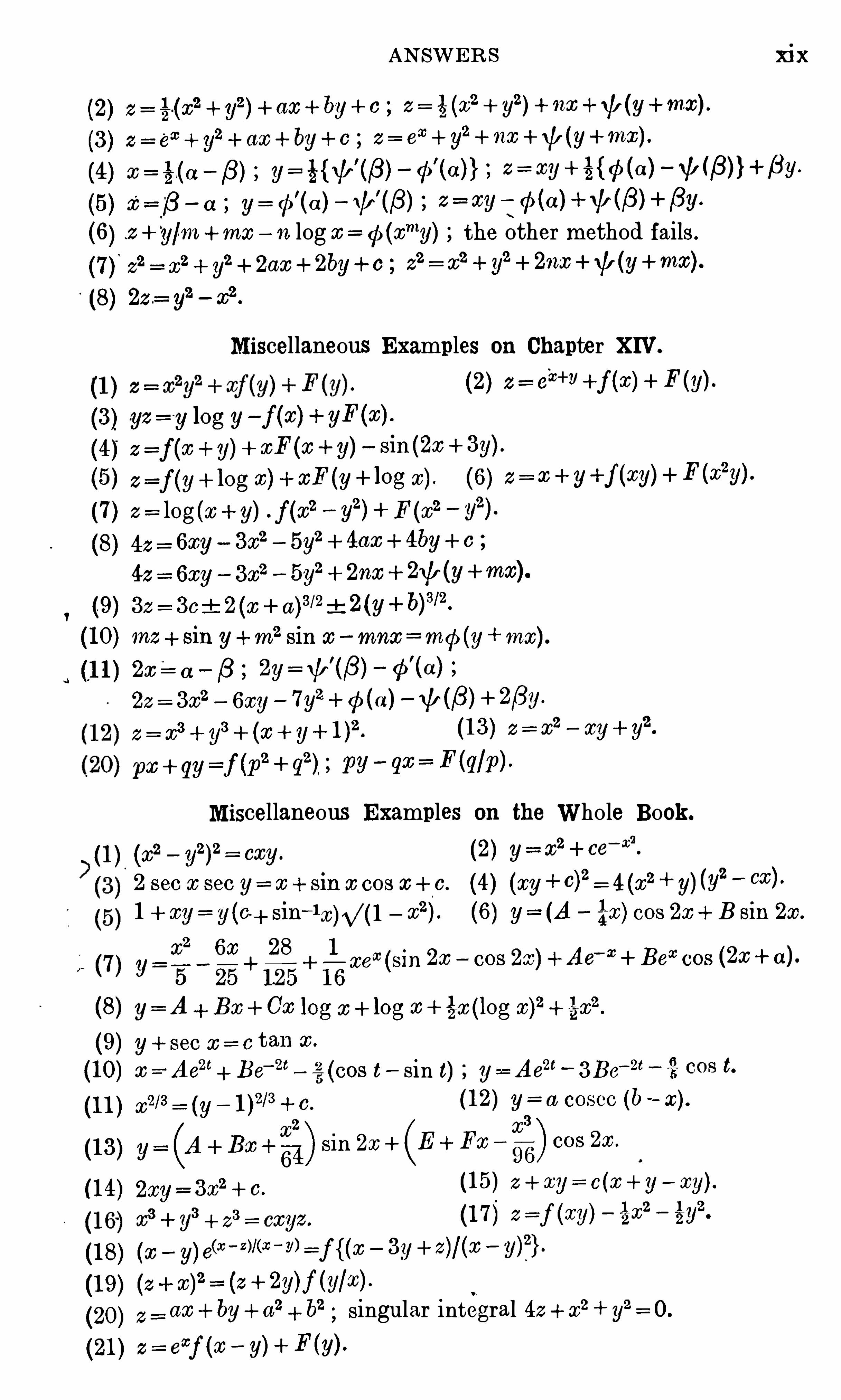
Y
ANSW ERS xix
2 =
) 22 = e2+ y
2 2 = 02+ y
2
4M ; z =
) 90
) z
=fl a y= GH
(2
(3
(5
(6 2 +‘
y/m+mx n log x= ¢(xm1 ) the other method fails .
(72 — x
2
a
+ y2 2
2 : x2 + y
2
— x2
Miscellaneous Examples on Chapter XIV.
(2) 2 = e2+y +f(x) F(y) .
(3) vz = 31 10s y
(4)
(5) x) + xF(y2
+ 10g x) . (6) 2 = F(x2y) .
(7) z = log<a:y) f(xz F(wzyz)
(8) 42 = 6xy 3x2 5y2+ 4cx 4by+ 0
42 6xy 3x2 5y2 2nx 2\b(y mx) .
(9) 32 30i 2(x at)” i 2(y b)3/2
.
(10) mz sin y m2 sin x mxx m¢(y mx) .
2w'
= a 2y=W(B)
22 = 3x2 — 6xy
(13) 2 = x2 — xy+ y
2.
1090+ q Py qw= F(q/vi
Miscellaneous Examples on the W hole Book.
(x2 (2)
2 sec x sec y= x sin x cos x+ 0. (4) (xy = 4(x
2y) (y
20x) .
1 + xy= y(c sin x
2) . (6 y= (A 4
x) cos 2x+ B sin 2x.
x2 6x 28 1
s (7) y= 2x — cos 2x) +Ae‘ 2+ Beaccos
5 25 125 1 6
(8) y= A Bx+ Cx log x+ log—x(log x)
2+ 7)—x
2.
(9) y see x= 0 tan x.
(10) x=-Ae2t Be
“ 2t§ (cos t Sin t) y
==Ae2‘ 3Be‘ 2t 1; cos t.
(1 1 ) x2/3 = (y (12) y= a coscc (b —x) .
x2 x
3
(13) y—
4> Sin 2x+(E + Fx cos 2x.
(14) 2xy= 3x2+ c . (15) 2 + xy= 0(x + y
— xy) .
x2+ y
3+ 2
3 = 0xy2 .2 =f (xy)
—
y2
w W “ y))2}
(19) y/w)
(20) 2 = ax+ by+ a2 b2 singular integral 42 + x2 y
“°= O.
(21 ) Z = 62
f (93

xx DIFFERENTIAL EQUATIONS
(22) 2 0x2 by 4a2 singular integral 162 x4 =0.
(23 ) F(w—y)
(24) (25)
(26) 2 fixy (27) 2 =f (2 x) F(2 y) .
(28) y(x+ c) = c2x ; singular solutions y= 0and
xn+1
(29) ay4 = (x+ b)
5. (30) y= A cos(n 1) B si n(m ).
(31 ) x2y2
(x cos a +_y sin a (32) y= — ge2xi s
“.
(33) x 0‘ "lt(0 cosM 6 sin M) 0cos (pt a ) ,
W here C’ A/V{(K2 K 2 p
2)2 4K 2p
2} , tan a 2Kp/(K
2 K 2 p2) ,
and a. and b ar e arbitrary constants.
(34) y=A cos (sin x) B sin (sin x) .
(35) (i) F = A log (r + z) B ;
(11) (j) A 0 d§+ B ,
6x Vte
(36) V A{15 5} (322
72) 3
1
7 (3524 302272
W here 72
x2y2
22
.
x x4
x5
(39) a = o(1 “fi rm
—
5+
x3
x6
x
2 ! a2 3 ! a3 6 ! a6+7 l
(41 ) y — x= c (xy 1 )
(42) y= (1 + x)“ — b(1 B (1 + x)
- 1 dx} .
If 2a is an integer , the integral can be evaluated byputting 2 (1 x) .
(43) (i) y = (1 — x2)(A B log x) ; (11) y= (1 + B log x) .
(44) (1 — x2) y= (a + b dx) 0
22 2. [Put log y u u = x is
sinh t.
a solution of the differential equation in u .]
(272 2) x2(2n 2)(2n 4)(2n 6) x
4
(45 ) — 1 )(2n — 2)(2n— 2)(2n — 4) x
3
+2(2n — l )(2n
(46) y= Ax5+ Ex2 + replacing by E.
0 x2
x4
(47> 4. (a)
<x>6
+a
(2)both converge within the circle [x] [a].

xxii D IFFERENTIAL EQUATIONS
(81 ) (i) (11) A= Io
— E/R ; (iii) I= E/R.
(82) I a cos (pt e) Ae‘ RUL
, W here a L2p2) , tan 6 :Lp/R,
and A is arbitrary .
a sin (pt e) , where tan e = (C'Lp
2 l )/pCR and
a = EO/vuow +p202R2} .
(85) x= A cos (t a ) B cos (3t— B) ; y= 2A cos (t (1 ) — 53 cos (St— B)
(86) a and b ar e the roots of X2(LN — M2) RS = O.
(91 ) x= A cos (pt 0) B cos (qt B) , y=A sin (pt 0) B sin(qt B) ,where 2p x
2) + x, 2g V(40
2K2) K .
d2z d(92)
d—
z
+ abz = ab0.
dt
(93) — 2,u2) makes the amplitude of the particular integral a
maximum, provided 2,u2 does not exceed 712
(94) x A0‘ “
cos (pt e) , W here p(97 (p 5Va
3r
—2cos 6. (98) y sin (pb/c) = ASin (xx/0)(cos pt a ) .
(100) C’cosh m(y h) cos (mx nt) .
(115 ) (vi ) u“.= A 2)
2+ B (
(viii ) use22<P cos
71—53+Q sin
(X) ux = A(— 9)x+B +
1—
1

INDEX
(The number s r efer to the pages. )
on of diffusivity ,
5 , 94, 209.
50, 126, 127 ,
Arbitrary functions, 49, 137 , 147 , 172.
Asymptotic series, 213 .
Auxiliary equation, xv , 26, 174, 216.
Bernoulli, xv , 12, 18.
Bernoulli’
s equation, 18.
Besse l, 1 10.
Besse l’s equation, 1 14, 1 16, 1 18, 120,215 .
Boole , xv .
Boundary conditions, 53 , 56.
Briot and Bouquet, xvi .Br odetsky
’
s graphical method, vi , 5 .
Bromwich, 209.
Cauchy, xvi , 121 , 124.
0-discr iminant, 67 , 1 55 .
Change of variables, 40, 6 1 , 79, 85, 91 ,93, 1 19, 120, 1 64 .
Characteristics, 6, 97 , 158.
Charpit, xvi, 162.
Charpit’
s method, 162.
Ch emistry, 206.
3hrysta1, xvi, 150.
3lair aut, xv, 76.
31air aut’
s form, 76, 79.
30mmon primitive , 10.
Jomplementary function, 29, 87 , 175 ,216.
Jomplete integral, 153.
Jomplete primitive , 4 .
30nditions of integrability, 139, 144 ,
191 , 193
Conduction of heat, 52, 53 , 57 , 58, 59,60, 212.
Confocal conics, 23, 79.
Conjugate functions, 24, 189.
Constant coefficients, xv, 25 , 49, 173 ,178, 212, 214, 216.
Constants, arbitrary , 2, 50, 126 , 127 ,214.
Convergence , xvi , 1 12, 124.
Corpuscle , path of a, 48.
Cross-ratio, 201 .
Cusp-locus, 68, 73 .
D’
Alembert, xv , 25 , 44, 49.
B arboux, xvi.
Definite Integrals, solutionby , 212, 213.
Degree , 2.
Depression of order, 81 .
Developable surface , 1 89.
Difference equations, 216 .
Difficulties, special, of partial di fferential equations , 5 1 .
Diffusion of salt, 60.
Discriminant, 67 , 7 1 , 155 .
Duality , 160, 161 , 189, 210.
Dynamics, 2, 24, 28, 36, 46, 47 , 50, 61 ,85 , 86, 190, 204 , 205 , 206, 207 , 208,
209, 210, 21 1 .
Earth, age of, 60, 212.
Einste in, 209.
Electr icity, 24, 29, 46 , 48, 58, 59, 134,203 , 204, 205 , 206 .
Eliminat ion, 2, 49, 50, 179.
Envelope , 66, 7 1 , 146, 155 .
Equivalence , 92.
Euler, xv , 12, 25 , 49.
Exact equations , 12,23 , 91 , 191 .
Existence theo r ems , 121 , 214 .
Facto r isation of the ope r ator, 86.
Falling body, 24, 86.
xxii i

DIFFERENTIAL EQUATIONS
(The numbers r efer to the pag es . )
Falling chain, 208.Finite di fferences, 215 , 216.
First order and first degree , ordinary ,12, 133 partial, 147 , 15 1 .
First order but higher degree , ordinary ,62, 65 ; partial, 153 , 162, 165 .
Fontaine , xv.
Forsyth, 150, 194.
Foucaul t’
s pendulum, 209.
Fourier, 54.
Fourier’s in tegral, 60.
Fourier’
s series, 54.
Frobenius, xvi , 109.
Frobenius’
method, 109, 127 .
Fuchs, xvi.Functions, arbitrary , 49, 137 , 147 , 172.
Gauss, 1 10.
General integr al, xvi , 137 , 147 , 149, 157 .
General solution, 4.
Geometry , 5 , 19, 65, 133 , 137 , 1 46, 173 ,188, 189.
Gour sat, xvi, 172, 194.
Graphical methods, 5 , 8.
Groups, xvi, 120, 194.
Hamilton’
s equations , 210.
Heat, 52, 53 , 57 , 58, 59, 60, 212.
Heaviside , 58, 61 .
Heun, 94.
Heun’
s nume r ical method, 104.
Hill, M. J . M vi, xv , xvi, 65 , 150, 155 ,
192, 194.
Homogeneous equations, xv , 14, 40, 44,83 , 144 , 17 1 , 173, 213 .
Homogeneous linear equations, 40, 44,17 1 , 173 .
Hydrodynamics, 208.
Hypergeometric equation, 1 19, 120.
Hypergeometr ic series , 92, 1 19.
Indicial equation, 109, 1 1 1 .
Initial conditions, 4 , 28, 53 .
Inspection, integration by , 12, 172.
Integrating factor, xv , 13 , 17 , 22, 23, 91 ,
199.
Integrability , 139, 144 , 191 , 193.
Integral equation, 96.
Intermediate integral, 181 .
Invariant, 92.
Jacobi, xvi, 165 .
Jacobi’
s Last Multiplier, 211 .
Jacobi’
s method, 165 , 193 , 210.
K elvin, 58 , 60, 212.
K lein, xvi .
K utta, 94, 104, 108.K utta
’s numer ical method, 104.
Maxwell’s equations , 59.
Mechanics, see Dynamics .
Membrane , vibrating , 190.
Monge , xvi , 172.
Monge’
s method, 1 81 , 1 83.
Multipliers, 135 , 210, 21 1 .
Lagrange , xv, 49, 81 , 162.
Lagrange’
s dyn amical equations , 210.
Lagrange’
s linear partial di fferentialequation, xvi, 147 , 1 5 1 , 158 , 192.
Laplace xvi.
Laplace s equation, 5 1 , 189, 190, 196,197 , 213 .
Last multiplier, 21 1 .
Laws of algebra , 30.
Legendre , 1 10.
Legendre ’s equation, 1 17, 120.
Le ibniz , xv.
Lie , v, xvi, 194.
Linear difference equations ,Linear equations (ordinari ), of the
first order , 16 , 214 ; of the secondorder, 86, 87 , 88, 109, 127 , 214, 215 ;with constant coefficients, xv, 25 ,214.
Linear equations (partial), of the firstorder, xvi , 50, 147 , 15 1 , 158, 192 ;with constant coe ffi cients, 49, 173 ,
178 , 212.
Linearly independent integrals, 216.
Lines of force , 24 , 134.
Lobatto, xv.
Newton, xv.
Node -locus, 68.
Non -integrable equations, 142.
Normal form , 91 , 92.
Normal modes of vibration, 204, 206.
Number of linearly independent integrals, 216.
Numerical approximation, 94 .
One integral used to find another, 87 .
136.
Operator D , 30, 44, 86 , 174, 214.
Operator 0, 44.
Orbits, planetary , 86, 209.
Order, 2.
Orthogonal trajector ies, xv , 20, 23 , 138 ,
189.
Oscillations , xv , 2, 28, 29, 36, 46 , 47 ,
48 , 50, 61 , 190, 203 , 204, 205 , 206 ,
207.
Copyright © 2022 FDOKUMEN