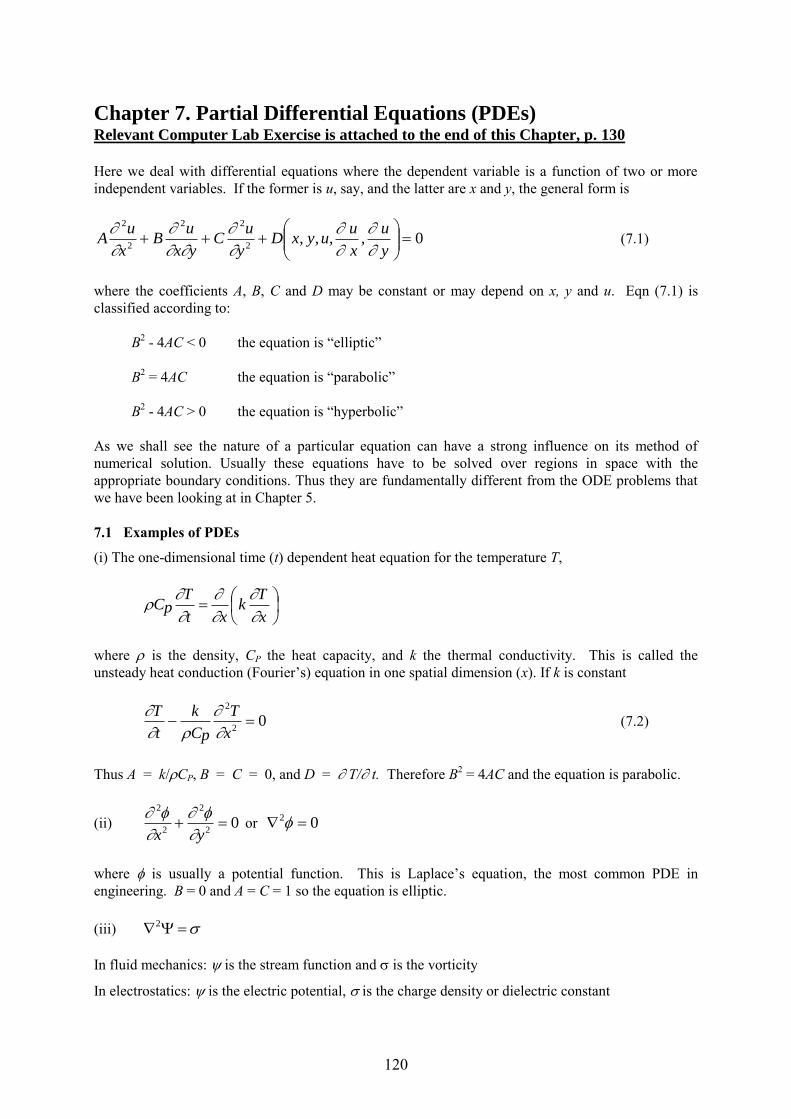
120

Chapter 7. Partial Differential Equations (PDEs) Relevant Computer Lab Exercise is attached to the end of this Chapter, p. 130

Here we deal with differential equations where the dependent variable is a function of two or more

independent variables. If the former is u, say, and the latter are x and y, the general form is

0,,,,2

22

2

2

y

u

x

uuyxD

y

uC

yx

uB

x

uA

(7.1)

where the coefficients A, B, C and D may be constant or may depend on x, y and u. Eqn (7.1) is

classified according to:

B2 - 4AC < 0 the equation is “elliptic”

B2 = 4AC the equation is “parabolic”

B2 - 4AC > 0 the equation is “hyperbolic”

As we shall see the nature of a particular equation can have a strong influence on its method of

numerical solution. Usually these equations have to be solved over regions in space with the

appropriate boundary conditions. Thus they are fundamentally different from the ODE problems that

we have been looking at in Chapter 5.

7.1 Examples of PDEs

(i) The one-dimensional time (t) dependent heat equation for the temperature T,

x

Tk

xt

TpC

where is the density, CP the heat capacity, and k the thermal conductivity. This is called the

unsteady heat conduction (Fourier’s) equation in one spatial dimension (x). If k is constant

02

2

x

T

pC

k

t

T

(7.2)

Thus A = k/CP, B = C = 0, and D = T/ t. Therefore B2 = 4AC and the equation is parabolic.

(ii) 02

2

2

2

yx

or 0 2

where is usually a potential function. This is Laplace’s equation, the most common PDE in

engineering. B = 0 and A = C = 1 so the equation is elliptic.

(iii) 2

In fluid mechanics: is the stream function and is the vorticity

In electrostatics: is the electric potential, is the charge density or dielectric constant

121

In elasticity: = z, is related to angle of twist of a cylinder in torsion

This is Poisson’s equation, which must also be elliptic as - is D in Eqn (7.1).

(iv) 2

2

2

2

x

y

W

Tg

t

y

where now T denotes tension in a stretched string, W is the mass per unit length and y is the

displacement. g is the acceleration due to gravity. This hyperbolic equation models a vibrating string

held rigidly at both ends.

7.2 Method of Numerical Solution Using Finite Differences

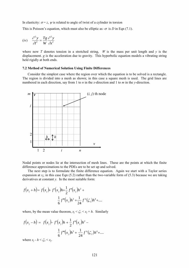
Consider the simplest case where the region over which the equation is to be solved is a rectangle.

The region is divided into a mesh as shown; in this case a square mesh is used. The grid lines are

numbered in each direction, say from 1 to n in the x-direction and 1 to m in the y-direction.

Nodal points or nodes lie at the intersection of mesh lines. These are the points at which the finite

difference approximations to the PDEs are to be set up and solved.

The next step is to formulate the finite difference equation. Again we start with a Taylor series

expansion at xj; in this case Eqn (5.2) rather than the two-variable form of (5.3) because we are taking

derivatives at constant y. In the most suitable form:

....24

1

6

1

2

1

4

1

3

2

hfhxf

hxfhxfxfhxf

iv

j

jjjj

where, by the mean value theorem, xj < 1 < xj + h. Similarly

....24

1

6

1

2

1

4

2

3

2

hfhxf

hxfhxfxfhxf

iv

j

jjjj

where xj - h < 2 < xj.

y

x

(i, j) th node

h

1 2 i n

h

1

2

j

m

122

i-1 i i+1

Denoting f(xj) as fj etc then two equations can be combined to give

2

2

11

12

12hff

h

fffiv

j

jjj

xj-1 < < xj+1

or 2

2

11 2hO

h

ffff

jjj

j

(7.3)

This is the central difference approximation to f(xj), the second derivative at xj with which you should

be familiar; Eqn (7.3) is just Eqn (4.13) from Section 4.2.

The two Taylor series can also be manipulated to give

211

2hO

h

fff

jj

j

(7.4)

the central difference approximation to f(xj). It has also appeared previously, as Eqn (4.15). Note

that (7.3) and (7.4) are accurate to the same order. Since very few PDEs have non-zero values of B,

Eqns (7.3) and (7.4) are usually all that is necessary to discretise the PDE at the appropriate nodes.

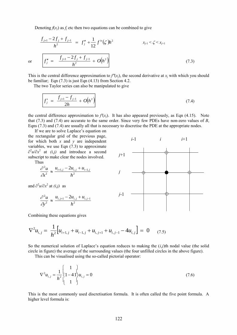
If we are to solve Laplace’s equation on

the rectangular grid of the previous page,

for which both x and y are independent

variables, we use Eqn (7.3) to approximate

2u/x

2 at (i,j) and introduce a second

subscript to make clear the nodes involved.

Thus

2

,1,,1

2

2 2

h

uuu

x

u jijiji

and 2u/x

2 at (i,j) as

2

1,,1,

2

2 2

h

uuu

y

u jijiji

Combining these equations gives

041

,1,1,,1,12,

2 jijijijijiji uuuuuh

u (7.5)

So the numerical solution of Laplace’s equation reduces to making the (i,j)th nodal value (the solid

circle in figure) the average of the surrounding values (the four unfilled circles in the above figure).

This can be visualised using the so-called pictorial operator:

01

1

4

1

11

,2,

2

jiji uh

u (7.6)

This is the most commonly used discretisation formula. It is often called the five point formula. A

higher level formula is:

j+1

j

j-1

123

0

141

4204

141

6

1,2,

2

jiji uh

u (7.7)

which has O(h6) error. We consider the implementation of these formulae by way of a simple

example with a small number of nodes and then discuss the more general case of a large number of

nodes.

7.3 Laplace’s Equation in a Rectangular Region

Example 7.1

A thin 10 x 20 cm plate has one of

its 10 cm edges held at 100°C

while the other edges are at 0°C.

The steady state temperature (T) is

described by

02

2

2

2

y

T

x

T

The simplest possible

discretisation is to use h = 5 cm

and have the three nodes as shown

in the figure below. We don’t have

to write the equations for nodes on

the boundary because we know

their temperature from the

boundary conditions. Note also that h2 does not appear in the final set of equations; it is simply

multiplied through. Using the sketch below, it is easy to apply the pictorial operator to node 1 to give

T2 + 0 + 0 + 0 - 4T1 = 0 (7.8a)

and

T3 + T1 + 0 + 0 - 4T2 = 0 (7.8b)

for node 2 and

100 + T2 + 0 + 0 - 4T3 = 0 (7.8c)

for node 3.

0 0

0 0 0

0

0 T1 T2 T3

100

T = 0C

T = 0C T = 100C

T = 0C y

x

124

Thus the numerical approximation to the PDE has resulted in a set of linear equations to be

solved. This is the common outcome of such methods.

The solutions are:

T1 = 1.786 C, T2 = 7.143 C, T3 = 26.786 C

which, as can be seen by comparison with the exact solutions whose determination does not concern

us,

T1,exact = 1.094 C, T2,exact = 5.489 C, T3.exact = 26.094 C

are remarkably accurate.

7.4 Methods for Large Number of Nodes

If we consider the Eqn (7.8) for three nodes and write them in a form similar to Jacobi iteration. Here

we get the (k+1)th iteration from the kth:

42

1

1

kk TT (7.9a)

431

1

2

kkk TTT (7.9b)

41002

1

3 kk TT (7.9c)

we have an example of Liebmann’s method. If we had used 1

1

kT in (7.9b) and 1

2

kT in (7.9c) we

would have the equivalent of Gauss-Seidel iteration.

In general, if u is the dependent variable then iteration is simply

4

1,1,,1,11

,

k

ji

k

ji

k

ji

k

jik

ji

uuuuu

(7.10)

for the Jacobi iteration, or

4

1

1,1,

1

,1,11

,

k

ji

k

ji

k

ji

k

jik

ji

uuuuu (7.11)

for the more rapidly converging Gauss-Seidel iteration. Eqn (7.10) can be written as

4

4 ,

1

1,1,

1

,1,1

,

1

,

k

ji

k

ji

k

ji

k

ji

k

jik

ji

k

ji

uuuuuuu (7.12)

where the bracketed term [] can be called a residual because

[ ] 0 as k

In some cases, convergence can be accelerated by rewriting (7.12) as

....,

1

, k

ji

k

ji uu (7.13)

is the “over relaxation factor” and its use is called “successive over relaxation” or SOR. Again

there is a strong analogy with the solution of linear equations: SOR in that case is described in Section

6.3 of these Notes.

125

The difference between (7.12) and (7.13) looks simple and appealing but in practice it is often

impossible to determine an optimum value of. In fact, some values of give poorer convergence

than = 1 used in Eqn (7.7). In mathematical terms, the determination of optimum is an

“eigenvalue” problem. In most cases 1 .

Note that there has been a further innovation in notation in this Section: the superscripts (k) and (k+1)

denote iteration number while the subscripts denote node number or position in space. To emphasise

the difference, the iteration number is parenthesised. The techniques for solving Eqns (7.10) to (7.13)

are those described in Chapters 2 and 6 where the iteration number is not parenthesised and there is

only one subscript on the dependent variable.

There are at least two ways that the methods of Chapters 2 and 6 can be applied in the present

context. Firstly, the (i,j) node numbering can be replaced by a single, (i), say, numbering as was done

in Section 7.3. The resulting system is banded and sparse and pivoting unnecessary because Eqn (7.6)

requires that the diagonal elements of the coefficient matrix have the general value of 4 and the off-

diagonal elements are unity.

The second method of solving these equations will now be described using (7.13) for the Example

7.1. The algorithm is given below. Note that,

all nodes are in the interior of the plate, so there is no need to be concerned with the corner

temperatures. In other words it does not matter whether the temperature at x = 20 cm, y = 0 is 0C

or 100C,

as in the implementation of Gauss-Seidel iteration there is no need to have a separate array for the

kth and (k+1)th iteration,

the convergence of the solution is determined by the maximum norm - see Section 2.10 - called

maxresid in the algorithm,

the temperature at all the nodes is initialised to 0C. This is not essential but is desirable.

Successive over-relaxation algorithm

In: Number of nodes in x direction, imax

Number of nodes in y direction, jmax

Maximum number of iterations, max

Convergence tolerance,

over relaxation factor,

Out: T(imax, jmax) the approximate steady state temperature

comment: use zeroth elements of T to contain boundary conditions

comment: initialise all other elements of T to zero

loop i = 1, imax +2

loop j = 1, jmax +2

T(i, j) = 0.0

end loop

end loop

loop j = 1, jmax + 2

T(imax+2, j) = 100.0

end loop

loop k = 1, max

maxresid = 0.0

loop i = 2, imax +1

loop j = 2, jmax +1

resid = [T(i+1,j) + T(i-1,j) + T(i,j+1) + T(i,j-1)]/4 - T(i,j)

if |resid| > maxresid then

maxresid = resid

endif

T(i,j) = T(i,j) + resid

126

end loop

end loop

if |maxresid| < then

exit with solution in T

endif

end loop

error: maximum number of iterations exceeded

Algorithm 7.1 Successive Over relaxation for Example 7.1

Example 7.2 Iterative solution of Example 7.1

The algorithm was programmed and used to investigate the effect of varying h on the accuracy of the

temperatures T1, T2, and T3 that were determined explicitly in Example 7.1. The results for a tolerance

of 10-5

are summarised in the following table. The results for h = 5 cm agree with the previously

determined direct solution to three decimal places. The errors, etc, are the difference between the

computed and exact temperature (whose determination is not described) and so are absolute errors.

Since the numerical scheme is based on the CD approximation, it should have O(h2) accuracy. That

means, in practice, that there should be a range of h over which /h2

etc are approximately constant.

This seems to be the case for the present calculations, eve though there is a considerable difference

between, say, the level of /h2 and /h

2.

h (cm) T1 (C) (C) /h2

5 1.7857 0.6914 0.0277

2.5 1.2894 0.1951 0.0312

1.25 1.1442 0.0499 0.0319

0.625 1.1069 0.0126 0.0323

Table 7.1(a) Summary of successive-over relaxation solutions for T1.

h (cm) T2 (C) (C) /h2 T3 (C) (C) /h

2

5 7.1429 1.6544 0.0662 26.7857 0.6913 0.0277

2.5 6.0194 0.5309 0.0849 26.2894 0.1950 0.0312

1.25 5.6317 0.1432 0.0916 26.1442 0.0500 0.0320

0.625 5.5250 0.0365 0.0934 26.1069 0.0125 0.0320

Table 7.1(b) Summary of successive-over relaxation solutions for T2 and T3.

h (cm) imax jmax opt no. iterations

5 3 1 1.1 7

2.5 7 3 1.3 14

1.25 15 7 1.6 30

0.625 31 15 1.7 79

Table 7.2 Optimum over relaxation factor and number of iterations.

To give an idea of the way in which opt, the optimum , and the number of iterations required for

convergence varies with the number of equations, a numerical search was undertaken for the three

values of h. The results are given in Table 7.2.

7.5 Boundary Conditions

If u is known along the boundary, as in our example, the problem is said to have Dirichlet

conditions. This is usually the easiest case to solve. If instead, the normal derivative is known along

127

the boundary then we have Neumann conditions. Often the normal derivative is related to a flux of

some physically important quantity, such as the heat transfer rate into a region.

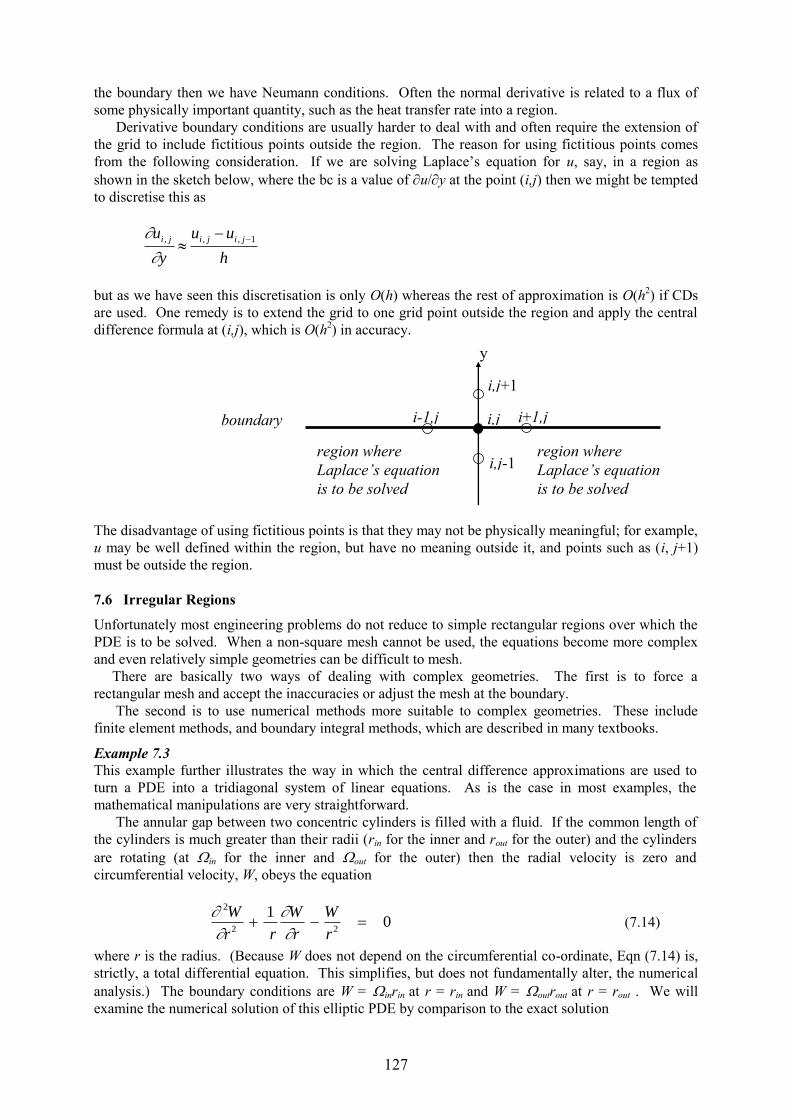
Derivative boundary conditions are usually harder to deal with and often require the extension of

the grid to include fictitious points outside the region. The reason for using fictitious points comes

from the following consideration. If we are solving Laplace’s equation for u, say, in a region as

shown in the sketch below, where the bc is a value of u/y at the point (i,j) then we might be tempted

to discretise this as

h

uu

y

u jijiji 1,,,

but as we have seen this discretisation is only O(h) whereas the rest of approximation is O(h2) if CDs

are used. One remedy is to extend the grid to one grid point outside the region and apply the central

difference formula at (i,j), which is O(h2) in accuracy.

The disadvantage of using fictitious points is that they may not be physically meaningful; for example,

u may be well defined within the region, but have no meaning outside it, and points such as (i, j+1)

must be outside the region.

7.6 Irregular Regions

Unfortunately most engineering problems do not reduce to simple rectangular regions over which the

PDE is to be solved. When a non-square mesh cannot be used, the equations become more complex

and even relatively simple geometries can be difficult to mesh.

There are basically two ways of dealing with complex geometries. The first is to force a

rectangular mesh and accept the inaccuracies or adjust the mesh at the boundary.

The second is to use numerical methods more suitable to complex geometries. These include

finite element methods, and boundary integral methods, which are described in many textbooks.

Example 7.3

This example further illustrates the way in which the central difference approximations are used to

turn a PDE into a tridiagonal system of linear equations. As is the case in most examples, the

mathematical manipulations are very straightforward.

The annular gap between two concentric cylinders is filled with a fluid. If the common length of

the cylinders is much greater than their radii (rin for the inner and rout for the outer) and the cylinders

are rotating (at in for the inner and out for the outer) then the radial velocity is zero and

circumferential velocity, W, obeys the equation

01

22

2

r

W

r

W

rr

W

(7.14)

where r is the radius. (Because W does not depend on the circumferential co-ordinate, Eqn (7.14) is,

strictly, a total differential equation. This simplifies, but does not fundamentally alter, the numerical

analysis.) The boundary conditions are W = inrin at r = rin and W = outrout at r = rout . We will

examine the numerical solution of this elliptic PDE by comparison to the exact solution

boundary i,j

i,j+1

i-1,j i+1,j

i,j-1 region where

Laplace’s equation

is to be solved

region where

Laplace’s equation

is to be solved

y

128

22

22

22

1)(ˆ

outin

outoutinin

outin

outin

rr

rrr

rrrrW (7.15)

If the annulus is divided radially into N interior points equally spaced h apart, where h = (rout -

rin)/(N+1), the central difference approximations for the first and second derivatives (Eqns 7.4 and

7.5) give for the ith point:

02

22

11

2

11

i

i

i

iiiii

r

W

hr

WW

h

WWW (7.16)

which can be simply rearranged as

011 iiiiii WlWdWu (7.17a)

for every i, which shows that applying the FD approximation has resulted in a tridiagonal system of

equations for the unknown Ws. To see the tridiagonality in another way, consider for example, N =

50, and i = 25; then the equation for W25 involves only W26 and W24. Changing the subscripts to

arguments, the coefficients, l(i), d(i), and u(i) are:

iii rhhiu

hrid

rhhil

2

111)(and,

21)(,

2

111)(

22 (7.17b)

For all values of i apart from i = 1 and N, the right hand side, b(i), of the equation is zero. At i = 1,

W(i-1) = inrin which is known and so must be moved to the right hand side. Thus b(1) = -inrin l(1).

A similar argument applies at i = N which gives b(N) = -outrout u(N). Therefore

)(2

11)(,

)(2

11)1(

hrhh

rNb

hrhh

rb

out

outout

in

inin

otherwise b(i) = 0. (7.18)

This completes the setting up of the tridiagonal system in the form of Eqn (2.29) from Section 2.9

with the only change in notation being that W(i) not x(i) are the unknowns in the present case.

A Fortran program was written to solve the tridiagonal equations using the Algorithms 2.5 and 2.6.

Two cases were considered:

Case 1: rin = 1.0 m, rout = 1.1 m, in = 1 rad/sec, and out = 3.636 rad/sec.

Case 2: rin = 0.01 m, rout = 0.5 m, in = 100 rad/sec, and out = 8 rad/sec.

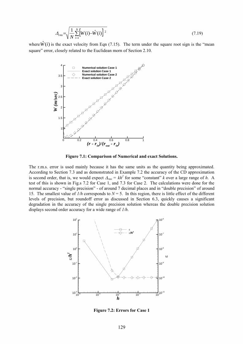
For these two cases, W is the same at each boundary: 1 m/sec at the inner surface and 4 m/sec at the

outer surface. Figure 7.1 shows the exact solution for both cases along with the numerical solutions

for N = 20. For Case 1, W is nearly linear in r so it is not surprising that the numerical solution is

more accurate. It is worth noting from the derivation of the CD formulae, that if W were linear or

quadratic in r, then the errors in the CD approximations, which involve third and higher derivatives,

would be zero. For Case 2, the velocity distribution is more complicated near the inner cylinder and

there the numerical solution is least accurate.

A way to formalise the level of error is to extend the use of “norms” that were introduced in

Section 2.10. A particularly useful measure is the “root mean square” error, rms, defined by

129

h

/h

2

10-6

10-5

10-4

10-3

10-210

-3

10-2

10-1

100

101

102

10-11

10-10

10-9

10-8

10-7

10-6

/h2

N

irms iWiW

N 1

2)(ˆ)(1

(7.19)

where )(ˆ iW is the exact velocity from Eqn (7.15). The term under the square root sign is the “mean

square” error, closely related to the Euclidean morn of Section 2.10.

Figure 7.1: Comparison of Numerical and exact Solutions.

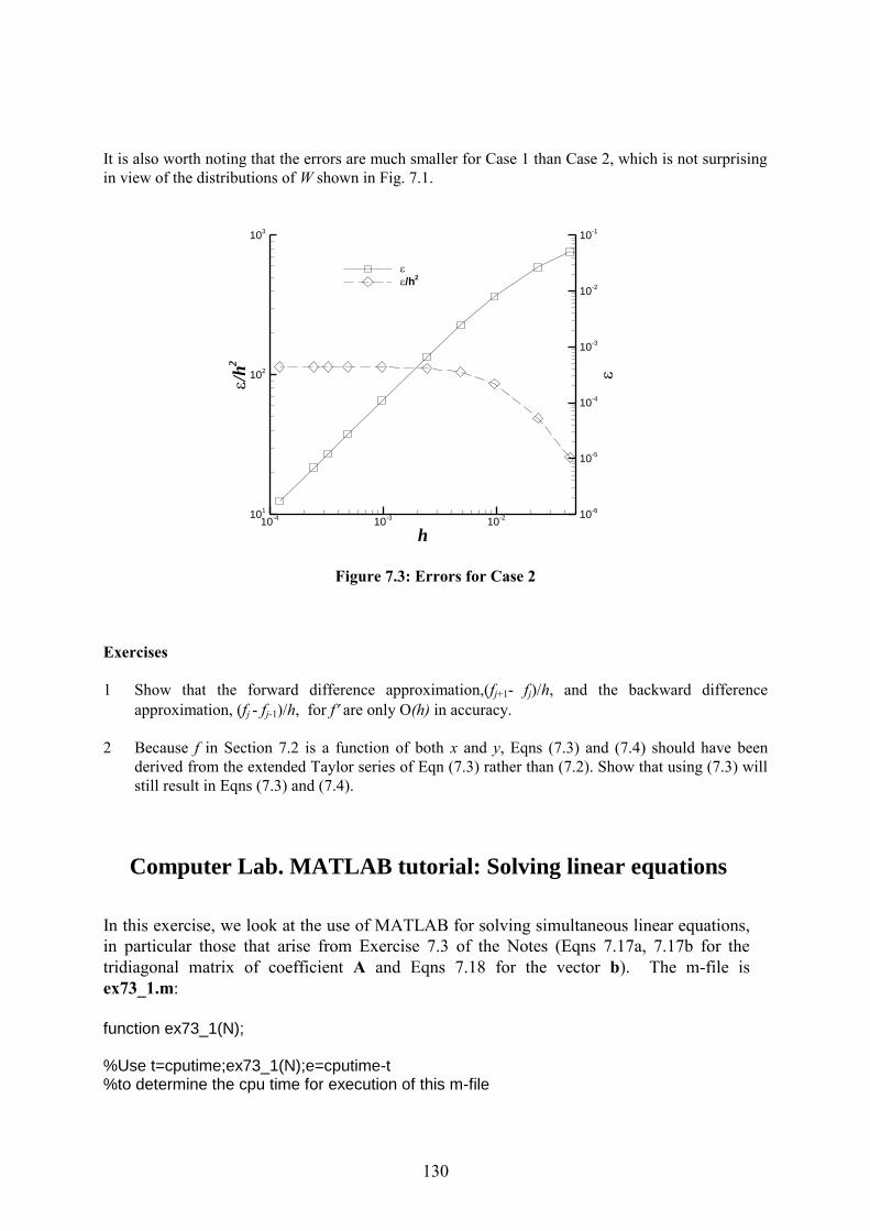
The r.m.s. error is used mainly because it has the same units as the quantity being approximated.

According to Section 7.3 and as demonstrated in Example 7.2 the accuracy of the CD approximation

is second order, that is, we would expect rms = kh2 for some “constant” k over a large range of h. A

test of this is shown in Fig.s 7.2 for Case 1, and 7.3 for Case 2. The calculations were done for the

normal accuracy - “single precision” - of around 7 decimal places and in “double precision” of around

15. The smallest value of 1/h corresponds to N = 5. In this region, there is little effect of the different

levels of precision, but roundoff error as discussed in Section 6.3, quickly causes a significant

degradation in the accuracy of the single precision solution whereas the double precision solution

displays second order accuracy for a wide range of 1/h.

Figure 7.2: Errors for Case 1

(r - rin)/(r

out- r

in)

W(m

/sec)

0 0.2 0.4 0.6 0.8 1

1

1.5

2

2.5

3

3.5

4Numerical solution Case 1

Exact solution Case 1

Numerical solution Case 2

Exact solution Case 2

130

h

/h

2

10-4

10-3

10-210

1

102

103

10-6

10-5

10-4

10-3

10-2

10-1

/h2

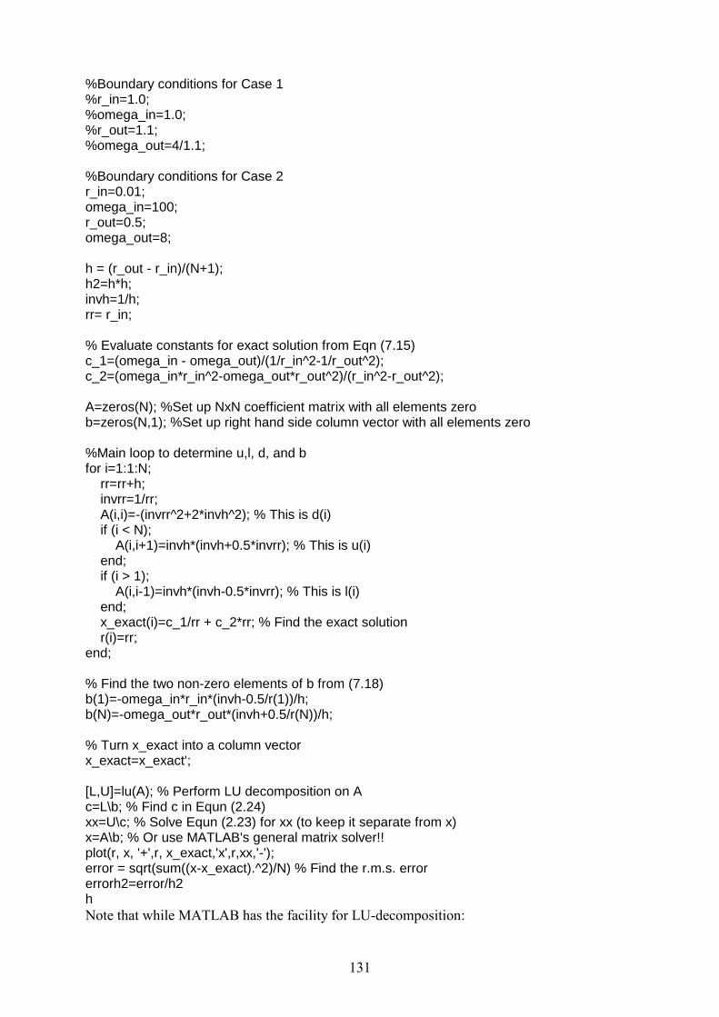
It is also worth noting that the errors are much smaller for Case 1 than Case 2, which is not surprising

in view of the distributions of W shown in Fig. 7.1.

Figure 7.3: Errors for Case 2

Exercises

1 Show that the forward difference approximation,(fj+1- fj)/h, and the backward difference

approximation, (fj - fj-1)/h, for f are only O(h) in accuracy.

2 Because f in Section 7.2 is a function of both x and y, Eqns (7.3) and (7.4) should have been

derived from the extended Taylor series of Eqn (7.3) rather than (7.2). Show that using (7.3) will

still result in Eqns (7.3) and (7.4).

Computer Lab. MATLAB tutorial: Solving linear equations

In this exercise, we look at the use of MATLAB for solving simultaneous linear equations,

in particular those that arise from Exercise 7.3 of the Notes (Eqns 7.17a, 7.17b for the

tridiagonal matrix of coefficient A and Eqns 7.18 for the vector b). The m-file is

ex73_1.m:

function ex73_1(N); %Use t=cputime;ex73_1(N);e=cputime-t %to determine the cpu time for execution of this m-file

131

%Boundary conditions for Case 1 %r_in=1.0; %omega_in=1.0; %r_out=1.1; %omega_out=4/1.1; %Boundary conditions for Case 2 r_in=0.01; omega_in=100; r_out=0.5; omega_out=8; h = (r_out - r_in)/(N+1); h2=h*h; invh=1/h; rr= r_in; % Evaluate constants for exact solution from Eqn (7.15) c_1=(omega_in - omega_out)/(1/r_in^2-1/r_out^2); c_2=(omega_in*r_in^2-omega_out*r_out^2)/(r_in^2-r_out^2); A=zeros(N); %Set up NxN coefficient matrix with all elements zero b=zeros(N,1); %Set up right hand side column vector with all elements zero %Main loop to determine u,l, d, and b for i=1:1:N; rr=rr+h; invrr=1/rr; A(i,i)=-(invrr^2+2*invh^2); % This is d(i) if (i < N); A(i,i+1)=invh*(invh+0.5*invrr); % This is u(i) end; if (i > 1); A(i,i-1)=invh*(invh-0.5*invrr); % This is l(i) end; x_exact(i)=c_1/rr + c_2*rr; % Find the exact solution r(i)=rr; end; % Find the two non-zero elements of b from (7.18) b(1)=-omega_in*r_in*(invh-0.5/r(1))/h; b(N)=-omega_out*r_out*(invh+0.5/r(N))/h; % Turn x_exact into a column vector x_exact=x_exact'; [L,U]=lu(A); % Perform LU decomposition on A c=L\b; % Find c in Equn (2.24) xx=U\c; % Solve Equn (2.23) for xx (to keep it separate from x) x=A\b; % Or use MATLAB's general matrix solver!! plot(r, x, '+',r, x_exact,'x',r,xx,'-'); error = sqrt(sum((x-x_exact).^2)/N) % Find the r.m.s. error errorh2=error/h2 h

Note that while MATLAB has the facility for LU-decomposition:

132

[L,U]=lu(A); % Perform LU decomposition on A

it cannot, apparently, deal with the particular case of tridiagonal systems for which there

should be no need to establish the full coefficient matrix A.

On the other hand, MATLAB easily deals with solving simultaneous equations using

“backslash” division as indicated by “\” rather than “/”:

c=L\b; % Find c in Equn (2.24) xx=U\c; % Solve Equn (2.23) for xx (to keep it separate from x) x=A\b; % Or use Matlab's general matrix solver!!

where all divisions are “backslash”, in other words, for the first line, L and b are known so

the backslash division finds c such that Lc = b. Note that these three lines actually solve

the equations twice, the first exploiting MATLAB’s LU decomposition features and the

second by numerical brute force. These matrix manipulations are a very powerful feature of

MATLAB.

After the equations are solved, the results are plotted and the r.m.s. error of the numerical

solution determined by comparison to the exact solution. Note haw the error is found using

term-by-term exponentiation of the vectors x and x_exact.

This m-file is executed by typing the command:

>> ex73_1(50)

for N = 50. Alternatively, to find out how much cpu time is required to solve the

equations:

>>t = cputime; ex73_1(50); e=cputime-t

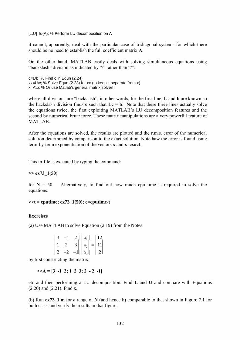
Exercises (a) Use MATLAB to solve Equation (2.19) from the Notes:

1

2

3

3 1 2 12

1 2 3 11

2 2 1 2

x

x

x

by first constructing the matrix

>>A = [3 -1 2; 1 2 3; 2 - 2 -1]

etc and then performing a LU decomposition. Find L and U and compare with Equations

(2.20) and (2.21). Find x.

(b) Run ex73_1.m for a range of N (and hence h) comparable to that shown in Figure 7.1 for

both cases and verify the results in that figure.

133

(c) Determine the cpu time required to run the m-file for a range of N. For each N you should

execute the m-file several times and find the average time.

(d) Determine whether it is more efficient computationally to solve the equations using LU-

decomposition or not. In other words, is it quicker to calculate xx or x? This will require

modifications to the m-file to first of all find xx only, and then x only. What do you conclude

from these results?