Volume 3, Issue 1 2008 Article 17

Chemical Product and ProcessModeling

Numerical Solution of Non-Linear AlgebraicEquations by Modified Genetic Algorithm

Mohammad Danish, Department of Chemical Engineering,Aligarh Muslim University, Aligarh - 202002 , U.P. , IndiaShashi Kumar, Chemical Engineering Department, Indian

Institute of Technology Roorkee, Roorkee - 247667 ,Uttarakhand, India

Surendra Kumar, Chemical Engineering Department ,Indian Institute of Technology, Roorkee, Roorkee - 247667,

Uttarakhand , India

Recommended Citation:Danish, Mohammad; Kumar, Shashi; and Kumar, Surendra (2008) "Numerical Solution of Non-Linear Algebraic Equations by Modified Genetic Algorithm," Chemical Product and ProcessModeling: Vol. 3: Iss. 1, Article 17.DOI: 10.2202/1934-2659.1122

Brought to you by | Indian Institute of Technology RoorkeeAuthenticated | 59.163.196.43

Download Date | 12/13/13 3:01 PM

Numerical Solution of Non-Linear AlgebraicEquations by Modified Genetic Algorithm

Mohammad Danish, Shashi Kumar, and Surendra Kumar

Abstract

Numerous unit operations in chemical and process engineering can be represented as asystem of non-linear algebraic equations, when modeled for steady state operation ,e.g. isothermaland non-isothermal operations of a series of CSTRs, batteries of evaporators, networks of variousseparation operations (flash drum, mixers), distillation, extraction and absorption columns, andpumps and piping networks etc. These governing equations are sometimes very difficult to solvedue to the nonlinear and uneven nature associated with them. The difficulty level increases whenthe resulting set of equations become flat near their zeros and thus derivatives based schemesmostly diverge or give poor results. Many a times, even a good initial guess in conventionalnumerical techniques do not guarantee to have a true solution and problem specific methods haveto be designed. This whole scenario can also be viewed as an optimization problem havingequality constraints only and casting the equations in the form of norm of function vector, whichformulates an objective function to be minimized. The true minimum thus found gives us thecorrect solution vector. Recently, Genetic Algorithms have been quite effectively used to solvemany complex engineering optimization problems. In continuation of our earlier research workwhere an elitist genetic algorithm was developed for the solutions of various difficult MINLPproblems (Danish et al. 2006a and b), this research work extends its application for the solution ofdifficult non-linear algebraic equations. A novel scheme of dynamic mutation parameter as afunction of fitness along with dynamic penalty has been proposed. The small value of mutationparameter in initial stages enables the algorithm to search globally, and the solution thus found isrefined by keeping its value higher in later generations. This new scheme is found to be veryeffective in the sense that the algorithm requires very small population size and comparativelylesser number of generations to give reasonably good solutions. To test the efficacy of algorithmwe have solved five sets of difficult non-linear algebraic equations (Dennis and Schnabel, 1983). Itis worthwhile to mention that one of these equations was having both its Jacobian and Hessian aszero, at its true solution. Applicability of the developed GA was also demonstrated by simulatingan industrial case study of triple effect evaporator used for concentrating the caustic soda solution(Zain and Kumar, 1996), which also poses difficulty during numerical simulation by Newton-Raphson method.

KEYWORDS: algebraic equations, numerical solution, optimization, genetic algorithm

Brought to you by | Indian Institute of Technology RoorkeeAuthenticated | 59.163.196.43

Download Date | 12/13/13 3:01 PM

1. Introduction

Algebraic equations are the basic and the most commonly encountered form of

any mathematical relation which arise in many areas of engineering and science.

Among them, non-linear equations are very interesting because of their peculiar

characteristics like existence of multiple solutions and non-convexities etc. In

chemical engineering too, a variety of non-linear algebraic equations are obtained

whenever any process is modelled in steady state condition and without any space

variation (Himmelblau and Bischoff, 1968; Bird et al., 2002). For example,

modelling of an assembly of CSTRs in isothermal or non-isothermal conditions,

sequence of evaporators, various mass transfer equipments like flash-drums,

mixers, distillation, extraction and absorption columns and pumps and piping

networks etc all yield non-linear algebraic or transcendental equations. Efforts

have been directed for devising fast and efficient numerical algorithm for solving

such equations. Different numerical techniques exist for their solutions e.g.

multivariable Newton-Raphson method and its variants and Broyden class of

methods etc (Dennis and Schnabel, 1983; Ferraris and Tronconi, 1986; Gupta,

1995); several system specific and optimization based approaches are also

available (Holland, C.D., 1975; Reklaitis et al., 1983; Floudas, 1995; Beigler et

al., 1997; Edgar et al., 2001). The choice of technique depends on the problem

and its difficulty level. Though, quick and accurate, these techniques require

auxiliary information such as existence and continuity of functions and their

derivatives, continuous updating of functions and derivatives, along with a good

initial guess, for the proper convergence of the method. Even then, in some

situations the equations may pose several difficulties in obtaining their solutions

because of the involvement of nonlinearities and unevenness. Moreover, the

flatness of equations at their zeros increases the complexity level and thus

derivatives based schemes mostly diverge or give poor results. Many a times,

even a good initial guess in these numerical techniques do not guarantee to have a

true solution and the problem specific methods have to be designed.

Recently, many optimization techniques based on probabilistic approaches

have been successfully employed e.g. Genetic Algorithms (Holland, J.H., 1975;

Goldberg, 1989; Michalewicz, 1992; Deb, 1995, 1999b, 2000a, 2001; Coello

Coello et al., 2002), Simulated Annealing (Kirkpatrick et al., 1983), Tabu search

(Glover, 1986; Hansen, 1986) and Ant Colony Optimization (Dorigo et al., 1996;

Wodrich and Bilchev, 1997; Dorigo and Stützle, 2005) etc. Of these, GAs have

been quite popular because of their stochastic approach and versatile nature.

Many engineering optimization problems especially Chemical Engineering

problems have been successfully solved using them (Androulakis and

Venkatasubramanian, 1991; Upreti and Deb, 1997; Nandsana et al., 2003; Hilbert

et al., 2006). Recently several multi-objective optimization problems of Chemical

1

Danish et al.: Numerical Solution of Non-Linear Algebraic Equations

Brought to you by | Indian Institute of Technology RoorkeeAuthenticated | 59.163.196.43

Download Date | 12/13/13 3:01 PM

Engineering have also been tackled by using GA (Bhaskar et al., 2000a & b;

Sankararao and Gupta, 2007a; Tarafder et al., 2007). Even new variants of GA

have been proposed and applied to optimize several industrial units e.g.

incorporation of jumping gene operator, a concept borrowed from Biological

Sciences (Kasat et al., 2003; Guria et al., 2005; Sankararao and Gupta, 2007 b).

Genetic Algorithms (Holland, J.H., 1975) are one of the meta-heuristic global

search algorithms. They are based on the concept of natural selection and exploit

the idea of survival of the fittest. Due to their simple and universal nature GAs

have successfully found wide ranging applications in Biology, Engineering,

Computer, Physical and Social Sciences, Pattern Recognition and Parallel

Processing etc and therefore a lot of study and research material is available on

them.

In our earlier work (Danish et al., 2006a and b), an elitist real GA with

dynamic penalty was developed for the solutions of difficult MINLP problems

(Grossmann and Sargent, 1979) which was then conveniently applied to solve

several multi-product batch plant design problems (MPBPD). The results obtained

were quite satisfactory. The work presented here, reports our experiences and the

pitfalls that arise when the above GA is used for solving difficult non-linear

algebraic equations, after formulating them into an optimization problem. After

performing many numerical experiments and understanding the behaviour, the

previous GA is slightly modified in order to obtain the true solution efficiently.

Moreover, it is also desired that this job is accomplished in lesser number of

generations with a small population size. The designed GA is then successfully

applied to solve five standard test problems and the results are compared with

those available in literature and a good agreement between them has been found.

Thereafter, to ensure the reliability of the modified GA, an industrial case study of

a triple effect evaporator system has been attempted. The obtained results are

compared and are found to be commensurable with the one available in literature.

This evaporator problem is found to be quite sensitive to the value of initial guess,

ordering of various equations and variables. Besides, convergence related

difficulties are also encountered when one solves it using Newton-Raphson

method (Zain and Kumar, 1996).

2. Modified genetic algorithm

From many of the numerical experiments done in our previous work, real GA was

found to be much more effective as compared to binary GA. Therefore, a real GA

with elitism operator was developed for MINLP problems; elitism operator was

incorporated so as to preserve the best individuals found so far. The major steps

involved in our earlier GA for the solutions of MINLP problems are briefly

discussed below; the details can be found in (Danish et al. 2006a and b).

2

Chemical Product and Process Modeling, Vol. 3 [2008], Iss. 1, Art. 17

DOI: 10.2202/1934-2659.1122

Brought to you by | Indian Institute of Technology RoorkeeAuthenticated | 59.163.196.43

Download Date | 12/13/13 3:01 PM

(i) A constant size population of real solution vectors, belonging to their

respective domains, is generated randomly.

(ii) Each of the generated members is assigned a fitness as per some

definition. Dynamic penalty is imposed if the solution does not follow

associated constraints or some other conditions.

(iii) By having a tournament between any two randomly chosen members,

selection of the winner for the mating pool is carried out.

(iv) Local search within the population is performed by simulated binary

cross-over (SBX) operator which exchanges the information (values)

between two randomly selected parent solutions so as to modify the

population.

(v) Thereafter, the modified population is operated by polynomial mutation

operator after some predefined mutation probability has happened.

(vi) Thus obtained new population is arranged in descending order of their

fitness. A specified percentage of best strings from the original

population, replaces the same numbers of strings from bottom in the new

population. A constant population size is maintained and the modified

population goes through steps (ii) to (vi) for further treatment. This

process continues until some terminating criteria are met.

With the above proposed algorithm, different MPBPD problems have been

fruitfully solved. Though, the algorithm is capable of finding true optima for

nonlinear equations, yet it encounters several problems related to true

convergence e.g. the values obtained are not precise or it took more generations to

obtain satisfactory results. Moreover, it is observed that the algorithm faces

difficulties for those non-linear algebraic systems where, (i) the true optimum is

lying on a flat surface and the fitness of near by solutions is not differing too

much and/or (ii) there are many good quality local optima in the very vicinity of

true solution. As shown in later sections, the conventional numerical techniques

also come across several difficulties in these kinds of problems e.g. the Jacobian

vanishing at the roots. Keeping these points in view, the previous algorithm is

slightly modified for successfully finding the solutions of difficult non-linear

algebraic equations. The key features of the present method include:

(i) Dynamic mutation parameter linked to the fitness of the population,

(ii) Imposition of the step wise dynamic penalty and

(iii) Existence of high local search by assigning a lower value to simulated

binary cross-over parameter c

η .

In this way, the developed GA is made suitable for non-linear equations

possessing flat profiles at their solutions i.e. zeros lie on an even surface. The

detailed descriptions of these changes are presented in the next section and the

algorithm is shown in Fig. 1.

3

Danish et al.: Numerical Solution of Non-Linear Algebraic Equations

Brought to you by | Indian Institute of Technology RoorkeeAuthenticated | 59.163.196.43

Download Date | 12/13/13 3:01 PM

Fig. 1 Modified Genetic Algorithm

Yes

No

GA Starts

Initialization of generation 0t =

Stop

Generations

completed ?

Population of real solution vectors ( xr

) are randomly generated in the defined domain min max

[ , ]X Xr r

.

In elitism operator, members coming through both the routes are compared and a

defined percentage of the best members from previous population directly replaces

the same number of poor members of the present population.

Values of the members are altered by polynomial mutation operator. This mutation

operator uses dynamic mutation parameter mη .

Information is exchanged between the selected strings by SBX-cross-over operator.

Evaluation of objective function ( )F xr

, imposition of step-wise penalty P and then obtaining

fitness f . Selection for mating pool by tournament selection operator.

Qualified strings along with their replica are stored in mating pool.

Specify GA parameters. Also, specify initial & final values of mutation parameters ,mi mfη η .

Members are sorted & stored as per their fitness.

Members are sorted & stored as per their

fitness.

Mutation parameter is dynamically updated by linking it to the best fitness of the

population & is moderated by taking the geometric mean of the last five values.

1

4( ) ( ) ;

tfitness fitness

mt mi mf mt mjj t

η η η η η−

= −

= = Π

4

Chemical Product and Process Modeling, Vol. 3 [2008], Iss. 1, Art. 17

DOI: 10.2202/1934-2659.1122

Brought to you by | Indian Institute of Technology RoorkeeAuthenticated | 59.163.196.43

Download Date | 12/13/13 3:01 PM

3. New solution strategy

The adopted methodology is basically based on varying the search level i.e. in the

beginning major search is initialized for finding the region of global optima.

Thereafter, search is gradually refined and in the end, very fine search is

maintained in a confined zone close to the global optima.

Mutation is a primary search operator and in the presently employed

polynomial mutation operator the search level is controlled by varying the

mutation probability index m

η . The magnitude of search level has been adjusted

by linking m

η with the fitness of the population such that m

η increases with the

fitness. This resulting approach is found to be quite fast and effective as compared

to the one with constant m

η . In addition, distance based stepwise increasing

penalty is imposed with the intention that a constant search power is maintained

even when the solutions are near their true values. In this type of penalty, the

amount of penalty during a known number of generations (constituting a step)

remains constant and the step size is fixed in advance such that the algorithm

hopefully finds a better solution. As the algorithm reaches near optima, the

population fitness increases which in turn raises m

η and thereby resulting in more

refining. Otherwise, if the algorithm moves away from global optima, then in the

next step of dynamic penalty, the increased penalty decreases the fitness which in

turn reduces m

η and eventually leads to a crude search. Both are somewhat

complementary to each other and are desirable when their overall effect increases

the fitness with generations.

3.1 Fitness evaluation

The actual values of variables in a solution vector are used to assess the

associated fitness. Many versions of fitness definitions are available (Costa and

Oliveira, 2001; Deb, 2001; Summanwar et al., 2002; Angira, and Babu, 2006;

Shopova and Vaklieva-Bancheva 2006). They are basically a measure of the

quality of a member. In case of a system of algebraic

equations ( ) 0 , . . 0, 1, 2...iE x i e E i n= = =rr r

, the zeros of equations can also be

determined by obtaining the zeros of square of the norm of equation vector i.e.

2

1

. ,n

T

ii

E E E E E=

= = ∑r r r r

. Hence, from the optimization point of view, this situation

can also be viewed as a minimization problem. Magnitude of this norm indicates

that how far the solution at that stage lies from zeros, and the fitness of a solution

5

Danish et al.: Numerical Solution of Non-Linear Algebraic Equations

Brought to you by | Indian Institute of Technology RoorkeeAuthenticated | 59.163.196.43

Download Date | 12/13/13 3:01 PM

vector xr

is defined to be inversely proportional to the deviation of its norm from

zero.

In the present approach, one of the equations is treated as an objective

function to be minimized while the rest are assumed to be equality constraints and

are penalized. Initially same weightage is given to all the equations so that the

region of global optimum may be searched in an unbiased way. Thereafter, only

constraint equations are penalized to have some relaxation and when the search is

confined to a very small but flat region near true root, all the equations are

penalized equally. Therefore, the value of objective function ( )F xr

of a member

in population at any generation is given by: 2

1( ) ;F x E P=r

+ (1a)

where,

2

2

2 3

2

; if 500

; else if 500< 4 10

n

ii

cn

ii

E t

Pt

a b E tb

=

=

≤∑= ×ℜ × ≤ ×∑

2

1

( ) ; otherwise

cn

ii

tF x a b E

b =

= ×ℜ × ∑

r(1b)

Thus, the objective function will be as follows:

2

1

( ) for 500n

ii

F x E t=

= ≤∑r

2 2 3

12

( ) 500< 4 10

cn

ii

tF x E a b E for t

b =

= + ×ℜ × ≤ ×∑

r and

2 3

1

( ) t > 4 10

cn

ii

tF x a b E for

b =

= ×ℜ × ×∑

r.

Though not shown, yet other stepwise dynamic penalty structures can also be

formed to get desired results; in general, they slightly affect the convergence of

the algorithm. The change in penalty with the generation number may be varied

by user as per convenience and depend on the problem. Since, the present GA is a

maximization code the following fitness definition has been adopted for finding

out the minima:

1

2

( ) ,( )

cf f x

c F x= =

+r

r (2)

min max,x X X ∈ r rr

Where, minXr

and maxXr

are the predefined domain of the variable vector xr

;

1 2&c c are constants and can be adjusted to magnify or reduce the fitness

6

Chemical Product and Process Modeling, Vol. 3 [2008], Iss. 1, Art. 17

DOI: 10.2202/1934-2659.1122

Brought to you by | Indian Institute of Technology RoorkeeAuthenticated | 59.163.196.43

Download Date | 12/13/13 3:01 PM

difference between two individuals (denominator should not be very small or

equal to zero). Although, equal values have been allotted to 1 2&c c in all the

problems so that f can be unity at optima however, the GA code has the

provision to assign different values to them. P is the stepwise dynamic penalty

imposed on solution vector for violating constraints. ( )t bℜ is the round off

operator which gives the integer value of the ratio t b and forces the penalty to

increase only after some generations. a is a small number and 1c Integer∈ ≥ .

These parameters should be chosen such that the bracketed term increases only

after the region of global optima is found. Its higher value may affect premature

convergence and its too low value may either put a very little penalty or may

expend more time.

3.2 Distribution index for cross-over probability c

η

Deb (2001) has shown that: (i) as the value of c

η decreases, the probability of

generating the faraway offspring from the parents increases and vice-versa and

(ii) for a fixed c

η the children have a spread which is proportional to that of the

parent solutions (see Appendix I). In later stages, the larger value of mutation

parameter m

η lessens the global search to a very large extent and the search is

mainly done by cross-over operator. Therefore, a lower value of c

η is assigned

from the very beginning which keeps the overall search to some non-zero level

even in final stages. Here, 0c

η = is chosen.

3.3 Dynamic mutation parameter m

η

It is well known that the mutation operator has a great impact on the search and

convergence of an algorithm. Therefore, its proper implementation is very

important. In the present work, the polynomial mutation has been chosen; the

search in this mutation operator is controlled by the parameter m

η (Deb, 2001). It

is observed that a value of m

η produces a perturbation of order 1/m

η in the

normalized decision variable space (Deb, 2001). The lower the value, higher is

the change in mutated variable and vice-versa. As shown later, the algorithm with

continuous variation in m

η outperformed the one with constant value both in

terms of convergence speed and solution quality. Since, in the beginning bigger

search is needed for finding the region of global optima so m

η is assigned a lower

value i.e. mi

η while in final stages its higher value i.e. mf

η results in a fine search

7

Danish et al.: Numerical Solution of Non-Linear Algebraic Equations

Brought to you by | Indian Institute of Technology RoorkeeAuthenticated | 59.163.196.43

Download Date | 12/13/13 3:01 PM

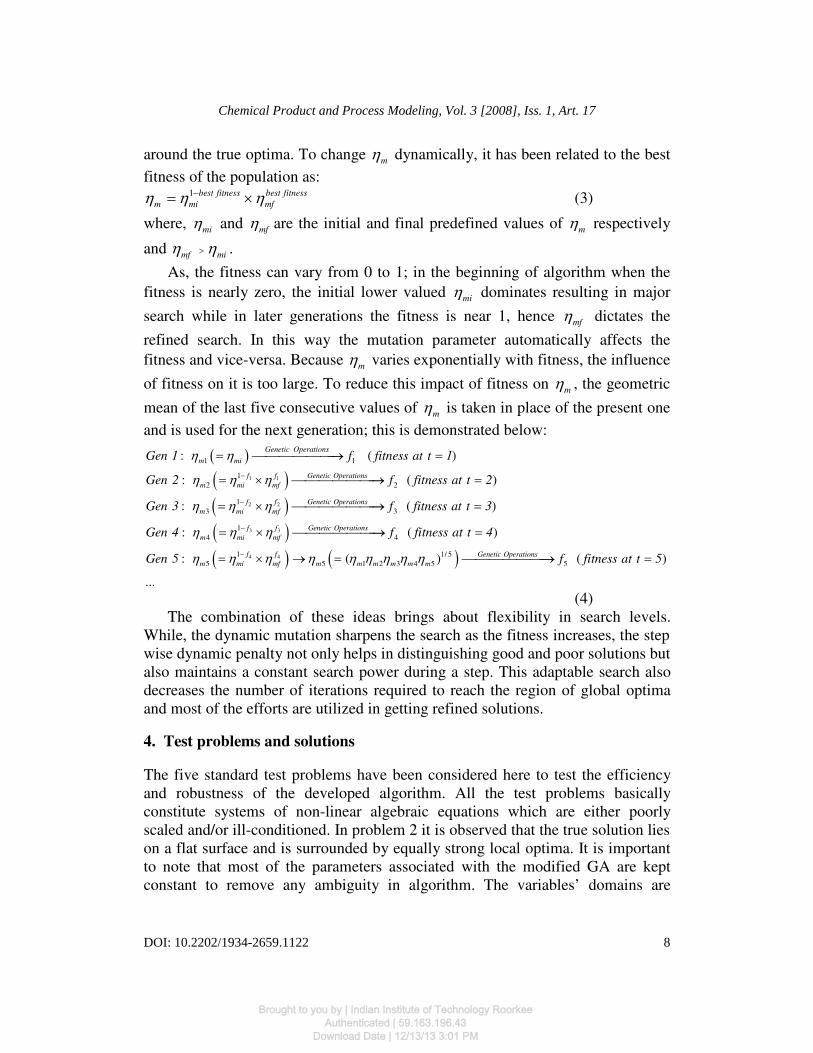
around the true optima. To change m

η dynamically, it has been related to the best

fitness of the population as: 1 best fitness best fitness

m mi mfη η η−= × (3)

where, mi

η and mf

η are the initial and final predefined values of m

η respectively

and mf mi

η η> .

As, the fitness can vary from 0 to 1; in the beginning of algorithm when the

fitness is nearly zero, the initial lower valued mi

η dominates resulting in major

search while in later generations the fitness is near 1, hence mf

η dictates the

refined search. In this way the mutation parameter automatically affects the

fitness and vice-versa. Because m

η varies exponentially with fitness, the influence

of fitness on it is too large. To reduce this impact of fitness on m

η , the geometric

mean of the last five consecutive values of m

η is taken in place of the present one

and is used for the next generation; this is demonstrated below:

( )

( )( )

1 1

2 2

1 1

1

2 2

1

3 3

: ( )

: ( )

: ( )

m mi

Genetic Operationsf f

m mi mf

Genetic Operationsf f

m mi mf

Genetic OperationsGen 1 f fitness at t 1

Gen 2 f fitness at t 2

Gen 3 f fitness at t 3

Ge

η η

η η η

η η η

−

−

= → =

= × → =

= × → =

( )( ) ( )

3 3

4 4

1

4 4

1 1/ 5

5 5 1 2 3 4 5 5

: ( )

: ( ) ( )

...

f f Genetic Operations

m mi mf

Genetic Operationsf f

m mi mf m m m m m m

n 4 f fitness at t 4

Gen 5 f fitness at t 5

η η η

η η η η η η η η η

−

−

= × → =

= × → = → =

(4) The combination of these ideas brings about flexibility in search levels.

While, the dynamic mutation sharpens the search as the fitness increases, the step

wise dynamic penalty not only helps in distinguishing good and poor solutions but

also maintains a constant search power during a step. This adaptable search also

decreases the number of iterations required to reach the region of global optima

and most of the efforts are utilized in getting refined solutions.

4. Test problems and solutions

The five standard test problems have been considered here to test the efficiency

and robustness of the developed algorithm. All the test problems basically

constitute systems of non-linear algebraic equations which are either poorly

scaled and/or ill-conditioned. In problem 2 it is observed that the true solution lies

on a flat surface and is surrounded by equally strong local optima. It is important

to note that most of the parameters associated with the modified GA are kept

constant to remove any ambiguity in algorithm. The variables’ domains are

8

Chemical Product and Process Modeling, Vol. 3 [2008], Iss. 1, Art. 17

DOI: 10.2202/1934-2659.1122

Brought to you by | Indian Institute of Technology RoorkeeAuthenticated | 59.163.196.43

Download Date | 12/13/13 3:01 PM

specified so as to contain only single true optimum otherwise it may lead to

another true solution if it exists. It is also experienced that the performance of

modified GA is unaffected with the size of the domain if it contains a lone global

optimum. All the test problems have been solved and checked a number of times

and the obtained results have been found to be within a reasonable tolerance

range. The tolerable variation in the results, in each run, is due to the stochastic

approach of the algorithm. The processing rate of the GA code with the specified

parameters (population, number of variables and equations etc.) for these test

problems is found to be approximately 10-13 generations per second on a

machine with Celeron M 1.4 GHz processor with 512 MB RAM.

Test problem 1

This is an extended Rosenbrock function with n=4 and results into a poorly scaled

objective function. But with the help of present GA the solutions have been easily

obtained. 2

1 2 110( ) 0E x x= − =

2 1(1 )E x= − 0=2

3 4 310( )E x x= − 0=

4 3(1 )E x= − 0=

or in compact vector form ( ) 0E x =rr r

.

Table 1: Results of test problem 1

Results S.

No.

Scaled

Variables

ix Exact Value

Value (present

work)

% Difference

1 1

x 1.0000000000 0.9999999853 0.0000014700

2 2x 1.0000000000 0.9999999705 0.0000029500

3 3x 1.0000000000 1.0000000024 0.0000002400

4 4x 1.0000000000 1.0000000047 0.0000004700

min max, ;x X X ∈ r rr

min [-10,-10,-10,-10];X =r

max [10,10,10,10];X =r

0.9999999911best

f = , 4

2 16

1

2.2385 10i

i

E −

== ×∑ .

GA parameters:

Generation = 35 10× , Population = 30 , 10%E = , 0.8

cp = , 0.5

mp = , 0

cη = ,

32 10mi

η = × , 810mfη = , 0.04, 100, 2a b c= = = , 3

1 10c−= , 3

2 10c−= .

9

Danish et al.: Numerical Solution of Non-Linear Algebraic Equations

Brought to you by | Indian Institute of Technology RoorkeeAuthenticated | 59.163.196.43

Download Date | 12/13/13 3:01 PM

Test problem 2

This is the Extended Powel Singular problem and is very interesting because both

the Jacobian and Hessian are singular matrices at the final root and hence,

Newton-Raphson technique for its solution cannot be applied. While running the

modified GA, it is also observed that as the population approaches near their

zeros, the reduction in value of one variable sharply increases the value of the

other and thus to achieve zero norm is very difficult. This problem has also been

solved using solver toolbox available in Microsoft EXCEL spreadsheet. As, can

be seen from Table 2, the results obtained from the modified GA are better than

those obtained from EXCEL software.

1 1 210E x x= + 0=

( )2 3 45E x x= − 0=

( )2

3 2 32E x x= − 0=

( )2

4 1 410E x x= − 0=

or ( ) 0E x =rr r

Table 2: Results of test problem 2

Results S.

No.

Scaled

Variables

ix Exact Value EXCEL Spreadsheet Value (present work)

1 1x 0.0000000000 -0.0001124362 0.0001470145

2 2x 0.0000000000 0.0000112593 -0.0000147017

3 3x 0.0000000000 -0.0001856214 0.0000469183

4 4x 0.0000000000 -0.0001856343 0.0000469070

42 -14

1

4.960503 10i

i

E=

= ×∑4

2 15

1

1.08266 10i

i

E −

== ×∑

min max, ;x X X ∈ r rr

min [-1,-1,-1,-1];X =r

max [1,1,1,1];X =r

0.999999913best

f = .

GA parameters:

Generation = 35.5 10× , Population = 30 , 10%E = , 0.8

cp = , 0.5

mp = ,

0c

η = , 32 10mi

η = × , 510mfη = , 0.4, 100, 2a b c= = = , 6

1 10c−= , 6

2 10c−= .

Test problem 3

The following set of equations includes the trigonometric functions. It is

important to note that the domain is specified in such a way that only (0, 0) is

10

Chemical Product and Process Modeling, Vol. 3 [2008], Iss. 1, Art. 17

DOI: 10.2202/1934-2659.1122

Brought to you by | Indian Institute of Technology RoorkeeAuthenticated | 59.163.196.43

Download Date | 12/13/13 3:01 PM

included in it as there are many other zeros for this system and GA may very

likely converge to one of them.

1 1 1 2cos 2sin cos 0E x x x= + − =

2 2 1 22 sin cos 3cos 2 0E x x x= − + − =

or ( ) 0E x =rr r

Table 3: Results of test problem 3

Results

S.

No.

Scaled

Variables

ix Exact Value

Value (present

work)

% Difference

1 1x 0.0000000000 0.0000000000 0.0000000000

2 2x 0.0000000000 0.0000000000 0.0000000000

min max, ;x X X ∈ r rr

min [-0.5,-0.5];X =r

max [0.5,0.5];X =r

1.0000000000best

f = , 2

2

1

0.0000000000i

i

E=

=∑ .

GA parameters:

Generation = 23 10× , Population = 30 , 10%E = , 0.8

cp = , 0.5

mp = , 0

cη = ,

32 10mi

η = × , 710mfη = , 0.4, 100, 2a b c= = = , 3

1 10c−= , 3

2 10c−= .

Test problem 4

This problem is obtained from Helical Valley function with n=3 and comprises of

transcendental and trigonometric functions. The very good quality results are

obtained in a few numbers of generations.

( )1 3 1 210 10 ( , )E x x xθ= − × 0=

( )2 2

2 1 210 1E x x= + − 0=

3 3E x= 0=

where,

1 21

1

1 2

1 21

1

1tan 0

2( , )

1 1tan 0

2 2

xif x

xx x

xif x

x

πθ

π

−

−

>

=

+ <

or ( ) 0E x =rr r

11

Danish et al.: Numerical Solution of Non-Linear Algebraic Equations

Brought to you by | Indian Institute of Technology RoorkeeAuthenticated | 59.163.196.43

Download Date | 12/13/13 3:01 PM

Table 4: Results of test problem 4

min max, ;x X X ∈ r rr

min [-10,-10,-10];X =r

max [10,10,10];X =r

1.0000000000best

f = , 3

2

1

0.0000000000i

i

E=

=∑ .

GA parameters:

Generation = 31 10× , Population = 30 , 10%E = , 0.8

cp = , 0.5

mp = , 0

cη = ,

32 10mi

η = × , 1010mfη = , 0.4, 100, 2a b c= = = , 3

1 10c−= , 3

2 10c−= .

Test problem 5

This is the well known Wood function. It is mentioned in the literature that it is a

difficult problem and is often used to test the algorithms for unconstrained

minimization. Table 5 depicts that the satisfactory results have been obtained in

less number of generations with a reasonably small population size.

( ) ( )2 22

1 2 1 1100 1E x x x= − + − 0=

( ) ( )2 22

2 4 3 190 1E x x x= − + − 0=

( ) ( )( )2 2

3 2 410.1 1 1E x x= − + − 0=

( ) ( )4 2 419.8 1 1E x x= − − 0=

or ( ) 0E x =rr r

Results S.

No.

Scaled

Variables

ix Exact Value

Value (present

work)

% Difference

1 1x 1.0000000000 1.0000000000 0.0000000000

2 2x 0.0000000000 0.0000000000 0.0000000000

3 3x 0.0000000000 0.0000000000 0.0000000000

12

Chemical Product and Process Modeling, Vol. 3 [2008], Iss. 1, Art. 17

DOI: 10.2202/1934-2659.1122

Brought to you by | Indian Institute of Technology RoorkeeAuthenticated | 59.163.196.43

Download Date | 12/13/13 3:01 PM

Table 5: Results of test problem 5

Results S.

No.

Scaled

Variables

ix Exact Value

Value (present

work)

% Difference

1 1x 1.0000000000 1.0000003949 0.0000394900

2 2x 1.0000000000 1.0000000702 0.0000070200

3 3x 1.0000000000 0.9999999790 0.0000021000

4 4x 1.0000000000 1.0000000463 0.0000046300

min max, ;x X X ∈ r rr

min [-10,-10,-10,-10];X =r

max [10,10,10,10];X =r

1.00000000best

f = , 4

2 21

1

2.6981 10i

i

E −

== ×∑ .

GA parameters:

Generation =31 10× , Population =30 , 10%E = , 0.8

cp = , 0.5

mp = , 0

cη = ,

32 10mi

η = × , 1010mfη = , 0.4, 100, 2a b c= = = , 3

1 10c−= , 3

2 10c−= .

4.1 Adjustment of parameter values

Tuning of parameters is a vital part of any GA but there are no general guidelines;

even if guidelines are available, they are problem specific (Mitchell, 1996). In the

present work, tuning has been done with the aim that the modified GA may have

effective and swift convergent properties. It is therefore intended that the proper

solution may be achieved in lesser number of generations with small population

size meanwhile, it is also desired that most of the parameters be kept constant to

avoid empiricism. The following propositions have been considered for fine

tuning of different parameters.

A reasonable amount of preservation is done by keeping the elitism parameter

E =10% of the population, so that the good solutions, found so far, are not lost by

various genetic operators (this parameter E should be in accordance with the

mutation probability otherwise GA will result in premature convergence). At the

same time, high cross-over and mutation probabilities are chosen so as to get

variety of solutions in a population at any generation. A lower value of the cross-

over probability distribution index i.e. 0c

η = for SBX-operator has been taken

since its small value permits far-away solutions in a population to be selected for

further processing and vice versa. In later converging stages when the global

search is diminishing due to larger m

η , this lower value of c

η keeps a higher local

search for the solutions and is very promising when the function is flat near its

true solution. This parameter is similar to m

η and the more its value, less is the

13

Danish et al.: Numerical Solution of Non-Linear Algebraic Equations

Brought to you by | Indian Institute of Technology RoorkeeAuthenticated | 59.163.196.43

Download Date | 12/13/13 3:01 PM

change in a variable. The distribution index for polynomial mutationm

η increases

from its initial value mi

η to final value mf

η , as the best fitness of the population

increases with generations and thereby refining the global search as the

population reaches near its true optimum (which is either surrounded by equally

competent local optima or the function becomes nearly flat in close

neighbourhood of the global optimum). The fitness parameters 1 2&c c , are

constants and can be adjusted to magnify or lessen the fitness difference between

two individuals (denominator should neither be very small nor equal to zero).

Their values should be such that a reasonable fitness difference is present between

the initial members, members near global optima and the final true solution.

Using the above guidelines for parameter setting, the algorithm is now used to

solve a system of triple effect evaporator used for concentrating the caustic soda

solution. It is important to mention that this problem faced convergence related

difficulties when solved by Newton-Raphson method; moreover, the convergence

also depends on the order of variables and equations during simulation and on the

value of initial guess (Zain and Kumar, 1996). To avoid these shortcomings Zain

and Kumar had proposed an improved solution strategy comprising of five

equations only. This was achieved by rearranging the present 12 modelling

equations into 7 uncoupled and 5 coupled equations. The seven uncoupled

equations were solved sequentially and the rest five coupled equations were

solved simultaneously. This system of 5 coupled equations is quite easy to solve.

In this way, the complete problem was simulated without any convergence related

difficulties. Though not shown here, the present and previous algorithms (Danish

et al., 2006a and b) are capable of solving this problem successfully when the

suggested strategy of five equations is followed. Using present GA the processing

rate for evaporator problem is found to be approximately 7 generations per second

on the earlier mentioned machine.

5. Industrial case study

The present evaporator problem consists of twelve nonlinear algebraic equations.

The interest in this problem lies because of the following reported observations:

(i) The equations are non-linear and coupled and present difficulties in

numerical simulations.

(ii) It has been reported (Zain and Kumar, 1996) that the order of variables

is important otherwise in some cases its Jacobian becomes ill

conditioned while solving by the Newton-Raphson technique leading to

divergence of the method.

(iii) Moreover, care should be taken in evaluating the derivatives

numerically. The use of proper weights in the relaxation strategy is of

utmost importance for getting the converged solution.

14

Chemical Product and Process Modeling, Vol. 3 [2008], Iss. 1, Art. 17

DOI: 10.2202/1934-2659.1122

Brought to you by | Indian Institute of Technology RoorkeeAuthenticated | 59.163.196.43

Download Date | 12/13/13 3:01 PM

5.1 Steady state modeling equations for triple effect evaporator system with forward feed arrangement

The governing non-linear and coupled algebraic equations have been taken from

the paper of Zain and Kumar and are reproduced below; the constitutive relations

are given in appendix II. The details of their derivation are given else where

(Holland, C.D., 1975).

First Effect:

1 1 0 0 1 1 1 1[ ( , ) ( , )] ( )[ ( ) ( , )] 0.0

F FF h T x h x V F L H h xτ λ τ τ− + − − − =

1 1 0 1 0 0( ) 0.0U A T Vτ λ− − =

1 1 1 1( ) ( ) 0.0m x T b x τ+ − =

1 10.0

FL x Fx− =

Second Effect:

1 1 1 2 2 1 1 1 1 2 2 2 2[ ( , ) ( , )] ( )[ ( ) ( )] ( )[ ( ) ( , )] 0.0L h x h x F L H h T L L H h xτ τ τ τ τ− + − − − − − =

2 2 1 2 1 1 1( ) ( )[ ( ) ( )] 0.0U A T F L H h Tτ τ− − − − =

2 2 2 2( ) ( ) 0.0m x T b x τ+ − =

2 20.0

FL x Fx− =

Third Effect:

2 2 2 3 3 1 2 2 2 2 3 3 3 3[ ( , ) ( , )] ( )[ ( ) ( )] ( )[ ( ) ( , )] 0.0L h x h x L L H h T L L H h xτ τ τ τ τ− + − − − − − =

3 3 2 3 1 2 2 2( ) ( )[ ( ) ( )] 0.0U A T L L H h Tτ τ− − − − =

3 3 3 3( ) ( ) 0.0m x T b x τ+ − =

3 30.0

FL x Fx− =

These modelling equations are either used for designing a new evaporator

system or for evaluating the performance of an existing one. Before solving these

equations, it is necessary to scale the variables to make them of the same order.

The scaling procedure is presented below:

(i) All the flow rates are divided by the feed flow rate.

(ii) All the temperatures are divided by the steam temperature.

(iii) All the equations are rearranged and normalized in the following form

by dividing the term with positive sign with the one having negative

sign.

1 0;i

term on LHS with ve signE

term on LHS with ve sign

+= − =

− i.e.

( ) ( )1 1 1 0 0 1 1 1 1[ ( , ) ( , )] / ( )[ ( ) ( , )] 1 0;

F FE F h T x h x V F L H h xτ λ τ τ= − + − − − =

2 1 1 1 2 2 1 1 1 1 2 2 2 2( [ ( , ) ( , )] ( )[ ( ) ( )]) /(( )[ ( ) ( , )]) 1 0;E L h x h x F L H h T L L H h xτ τ τ τ τ= − + − − − − − =

3 2 2 1 2 1 1 1( ) /(( )[ ( ) ( )]) 1 0;E U A T F L H h Tτ τ= − − − − =

15

Danish et al.: Numerical Solution of Non-Linear Algebraic Equations

Brought to you by | Indian Institute of Technology RoorkeeAuthenticated | 59.163.196.43

Download Date | 12/13/13 3:01 PM

4 2 2 2 3 3 1 2 2 2 2 3 3 3 3( [ ( , ) ( , )] ( )[ ( ) ( )]) /(( )[ ( ) ( , )]) 1 0;E L h x h x L L H h T L L H h xτ τ τ τ τ= − + − − − − − =

5 3 3 2 3 1 2 2 2( ) /(( )[ ( ) ( )]) 1 0;E U A T L L H h Tτ τ= − − − − =

6 1 1 0 1 0 0( ) /( ) 1 0;E U A T Vτ λ= − − =

7 1 1 1 1( ( ) ( )) / 1 0;E m x T b x τ= + − =

8 1 1/( ) 1 0;

FE L x Fx= − =

9 2 2 2 2( ( ) ( )) / 1 0;E m x T b x τ= + − =

10 2 2/( ) 1 0;

FE L x Fx= − =

11 3 3 3 3( ( ) ( )) / 1 0;E m x T b x τ= + − =

( )12 3 3/ 1 0;

FE L x Fx= − =

Operating conditions:

Feed (kg/hr) : 25000.000

Feed concentration (% weight fraction) : 8.000

Feed temperature ( oC ) : 110.000

Area of 1st, 2

nd and 3

rd effect (m

2) : 85.34, 77.45 & 69.74

Input steam temperature ( oC ) : 165.01496

Last effect temperature ( oC ) : 33.545586

5.2 Results of triple effect evaporator system for different parameter values

For the above operating conditions, the evaporator problem has been solved using

proposed GA for various parameter settings. The results obtained have been

compared with the one obtained by Zain & Kumar (shown in Table 6) and the

effects of different schemes on the results are shown and discussed below.

Different schemes include: dynamic mutation vs. constant mutation (both in the

presence of dynamic penalty), dynamic mutation vs. constant mutation (both in

the absence of dynamic penalty) and the effect of elitism on the convergence. The

simulation results have been summarized in Table 7 and depicted in the form of

two types of plots (shown in Figs. 2-7). The two types of plots are fitness vs.

generations and logm

η vs. generations.

Table 7 shows the results of triple effect evaporator system solved by the

present algorithm. The obtained results have been categorized into different cases

for various parameters’ values. For all the cases, parameters namely

Population=30, 0.8c

p = , 0.5m

p = , 0c

η = , 0.2,a = 100,b = 2c = , 1 1c = , and

2 1c = have been kept constant and mentioned above the Table 7. From Table 7

and Figs. 2-7, following observations may be made:

1. Cases 1(a) & 1(c) represents the successful runs when m

η is changed

dynamically. Case 1(b) is just a replica of Case 1(a) and has been included to

16

Chemical Product and Process Modeling, Vol. 3 [2008], Iss. 1, Art. 17

DOI: 10.2202/1934-2659.1122

Brought to you by | Indian Institute of Technology RoorkeeAuthenticated | 59.163.196.43

Download Date | 12/13/13 3:01 PM

show one of those very few runs which failed (due to probabilistic nature of

algorithm). Although case 1 (b) is taken as unsuccessful but values of

variables obtained after 5,000 generations are quite close to true solution

values. If one continues above 5,000 generations, he is likely to approach to

the solution vector. This is evident from case 1(c) where number of

generations have been increased to 20,000 and for this case best fitnessbest

f =1

and12

2 18

1

10i

i

E −

==∑ and the run is considered as extremely successful.

Table 6: Comparison of results for triple effect evaporator system

Results

(Present Study)

S. No.

Scaled

Variables

ˆi

x

Results

(Zain and Kumar)

Case: 1(a) Case: 1(c)

1 1 1ˆ /x L F= 0.7630796087486242 0.763108 0.763079

2 2 1ˆ /

ox T T= 0.8317171073593507 0.831658 0.831717

3 3 2ˆ /x L F= 0.5041591682625670 0.504201 0.504158

4 4 2ˆ /

ox T T= 0.6364335950739348 0.636369 0.636434

5 5 3ˆ /x L F= 0.2260926694242861 0.226139 0.226092

6 6 1x̂ x= 0.1048383406957922 0.104835 0.104838

7 7 1ˆ /

ox Tτ= 0.8524147665486763 0.852427 0.852415

8 8 2x̂ x= 0.1586800459777299 0.158668 0.15868

9 9 2ˆ /

ox Tτ= 0.6711675626252620 0.671123 0.671168

10 10 3x̂ x= 0.3538372128725376 0.353765 0.353838

11 11 3ˆ /

ox Tτ= 0.3220719571752862 0.322027 0.322073

12 12ˆ /

ox V F= 0.3023499143374576 0.302324 0.30235

bestf = - 0.990448 1

122

1i

i

E=

=∑ 3.53718 × 10-11

9.64 × 10-9

3.01 × 10-18

2a. For cases 2-4, m

η is kept constant with generations and as evident from the

value of norm shown in Table 7, the runs for cases 2-4 are declared as

unsuccessful. Though the fitness curve (Fig. 2) for case 4 seems to reach

unity, yet the norm value is unsatisfactory, this is because there was no

penalization and it can be seen from equations 1 & 2 that in the absence of

penalty fitness will be very near to unity for this value of norm. An important

point to note is that constant m

η has been used with and without dynamic

17

Danish et al.: Numerical Solution of Non-Linear Algebraic Equations

Brought to you by | Indian Institute of Technology RoorkeeAuthenticated | 59.163.196.43

Download Date | 12/13/13 3:01 PM

penalty and the presence or absence of dynamic penalty does not significantly

improve the results if m

η is kept constant.

2b. Cases 4, 5 & 6 indicate that dynamic m

η has been helpful in obtaining the

true solution within 5,000 generations even without dynamic penalty.

3. Comparing cases 1(a) & 5, one can find that the inclusion of dynamic penalty

further improves the quality of results.

min maxˆ , ;x X X ∈ r r r

min [0, 0.1, 0, 0.1, 0, 0, 0.1, 0, 0.1, 0, 0, 0.1];X =r

max [1,1,1,1,1,1,1,1,1,1,1,1];X =r

Table 7: Results of triple effect evaporator system for different cases

(GA parameters: Population = 30 , 0.8c

p = , 0.5m

p = , 0c

η = , 0.2, 100, 2a b c= = = ,

11c = ,

21c = )

Case

Number Parameters Used

Best

fitness

bestf

Square of

norm 12

2

1i

i

E=∑

Remarks

1(a)

GA parameters:

Generation = 35 10× , 10%E = , 32 10

miη = × ,

1010

mfη =

Penalty structure:

if 200t ≤12

2 2

12

ˆ( ) ;ii

F x E E=

=r

+ ∑

else if 200 500t< ≤

122 2

12

ˆ( ) ;

c

ii

tF x E a b E

b =

= + ×ℜ × ∑

r

else

122

1

ˆ( ) ;

c

ii

tF x a b E

b =

= ×ℜ × ∑

r

.

0.990448 9.64E-09

Dynamic mutation with

step wise dynamic

penalty has been used.

Run is taken as

Successful.

1(b) Every thing same as Case 1(a) 0.018113 5.42E-05

Dynamic mutation with

step wise dynamic

penalty has been used.

Run is taken as

Unsuccessful.

1(c) Every thing same as Case 1(a)

except Generation = 320 10× 1 3.01E-18

Dynamic mutation with

step wise dynamic

penalty has been used.

Run is taken as

extremely successful.

18

Chemical Product and Process Modeling, Vol. 3 [2008], Iss. 1, Art. 17

DOI: 10.2202/1934-2659.1122

Brought to you by | Indian Institute of Technology RoorkeeAuthenticated | 59.163.196.43

Download Date | 12/13/13 3:01 PM

Table 7 continued

Case

Number Parameters Used

Best

fitness

bestf

Square of

norm 12

2

1i

i

E=∑

Remarks

2

Every thing same as Case 1(a)

except 3

2 10 .mi mf

consttη η= = × = 0.011566 8.55E-05

Constant mutation with

step wise dynamic

penalty has been used.

Run is taken as

unsuccessful.

3

Every thing same as Case 1(a)

except 3

5 10 .mi mf

consttη η= = × = 0.049236 1.93E-05

Constant mutation with

step wise dynamic

penalty has been used.

Run is taken as

unsuccessful.

4

Every thing same as Case 1(a)

except 3

5 10 .mi mf

consttη η= = × = and

with out any penalty.

0.999987 1.3E-05

Constant mutation

without any penalty has

been used.

Run is taken as

unsuccessful.

5 Every thing same as Case 1(a) but

with out any penalty.

0.999999

553 4.47E-07

Dynamic mutation

without any penalty has

been used.

Run is taken as

successful.

6

Every thing same as Case 1(a)

except 3

10 10 .mi mf

consttη η= = × = 0.255146 2.92E-06

Constant mutation with

step wise dynamic

penalty has been used.

Run is taken as

successful.

7

Every thing same as Case 1(a)

except

20%E =

0.909465

382 9.95E-08

Dynamic mutation with

step wise dynamic

penalty has been used.

Run is taken as

successful.

8

Every thing same as Case 1(a)

except

30%E =

0.648286

531 5.43E-07

Dynamic mutation with

step wise dynamic

penalty has been used.

Run is taken as

successful.

9

Every thing same as Case 1(a)

except

50%E =

0.477512

096 1.09E-06

Dynamic mutation with

step wise dynamic

penalty has been used.

Run is taken as

successful.

19

Danish et al.: Numerical Solution of Non-Linear Algebraic Equations

Brought to you by | Indian Institute of Technology RoorkeeAuthenticated | 59.163.196.43

Download Date | 12/13/13 3:01 PM

Table 7 continued

4. From the results of cases 7-10 one concludes that enhancement of E (from

20%-75%) has adverse effect on the convergence of the solution with in pre-

specified generations.

5. In fitness vs. generation plots of all the cases shown in Figs. 2-4 (except for

cases 4 and 5), the sudden decrease in fitness signifies the abrupt increase in

penalty while increase in fitness indicates that the algorithm has found some

equally good solutions. In cases 4 and 5 there was no penalization and thus

the fitness never decreased. All these behaviours are also visible in logm

η vs.

generation plots shown in Figs. 5-7 for respective cases. Due to exponential

dependency of m

η on fitness the plot of logm

η vs. generations bear the same

pattern as shown in Figs. 2 - 4.

In the light of above findings one can conclude that algorithm with dynamic

mutation outperformed the algorithm with constant mutation irrespective of the

amount of penalty. Inclusion of dynamic penalty further boosts the performance.

Moreover, higher value of elitism is undesirable as it renders the algorithm to

converge prematurely. It can be seen that the result of case 1(c) were much better

than those of Zain & Kumar respectively, though it took 20000 generations.

Case

Number Parameters Used

Best

fitness

bestf

Square of

norm 12

2

1i

i

E=∑

Remarks

10 Every thing same as Case 1(a) except

75%E = 1.314E-07 7.609473982

Dynamic

mutation with

stepwise

dynamic penalty

has been used.

Run is taken as

failed.

20

Chemical Product and Process Modeling, Vol. 3 [2008], Iss. 1, Art. 17

DOI: 10.2202/1934-2659.1122

Brought to you by | Indian Institute of Technology RoorkeeAuthenticated | 59.163.196.43

Download Date | 12/13/13 3:01 PM

0

0.1

0.2

0.3

0.4

0.5

0.6

0.7

0.8

0.9

1

0 500 1000 1500 2000 2500 3000 3500 4000 4500 5000

Generations

Best fitn

ess

case:1a

case:1b

case:2

case:3

case:4

case:5

0

0.1

0.2

0.3

0.4

0.5

0.6

0.7

0.8

0.9

1

0 500 1000 1500 2000 2500 3000 3500 4000 4500 5000

Generations

Best fitn

ess

case:6

case:7

case:8

case:9

case:10

Fig. 2 Best fitness vs. generation plots

Fig. 3 Best fitness vs. generation plots

21

Danish et al.: Numerical Solution of Non-Linear Algebraic Equations

Brought to you by | Indian Institute of Technology RoorkeeAuthenticated | 59.163.196.43

Download Date | 12/13/13 3:01 PM

0

0.1

0.2

0.3

0.4

0.5

0.6

0.7

0.8

0.9

1

0 2000 4000 6000 8000 10000 12000 14000 16000 18000 20000

Generations

Best fitn

ess

case:1c

3.00E+00

4.00E+00

5.00E+00

6.00E+00

7.00E+00

8.00E+00

9.00E+00

1.00E+01

0 500 1000 1500 2000 2500 3000 3500 4000 4500 5000

Generations

Log

(ηm)

case:1a

case:1b

case:2

case:3

case:4

case:5

Fig. 4 Best fitness vs. generation plots

Fig. 5 Log(ηm) vs. generation plots

22

Chemical Product and Process Modeling, Vol. 3 [2008], Iss. 1, Art. 17

DOI: 10.2202/1934-2659.1122

Brought to you by | Indian Institute of Technology RoorkeeAuthenticated | 59.163.196.43

Download Date | 12/13/13 3:01 PM

3

4

5

6

7

8

9

10

0 500 1000 1500 2000 2500 3000 3500 4000 4500 5000

Generations

case:6

case:7

case:8

case:9

case:10

Log

(ηm)

3

4

5

6

7

8

9

10

0 2000 4000 6000 8000 10000 12000 14000 16000 18000 20000

Generations

case:1c

Log

(ηm)

Fig. 6 Log(ηm) vs. generation plots

Fig. 7 Log(ηm) vs. generation plots

23

Danish et al.: Numerical Solution of Non-Linear Algebraic Equations

Brought to you by | Indian Institute of Technology RoorkeeAuthenticated | 59.163.196.43

Download Date | 12/13/13 3:01 PM

6. Conclusions

A modified real elitist GA with dynamic mutation parameter and stepwise

dynamic penalty has been developed for the solutions of non-linear algebraic and

transcendental equations with the aim that the solutions may be obtained in lesser

generations with small population size. This problem is attacked by transforming

the system of non-linear equations into an optimization problem and thereafter,

the associated global optima is found with the help of modified GA. To make the

GA adaptable for such situations, following changes have been incorporated: (i)

The mutation parameter has been forced to update continuously with generation

by linking it to the fitness of the best individual of a population in a generation.

(ii) Step wise dynamic penalty is imposed on the solutions, which do not satisfy

the system. It is observed that with the above modifications the performance of

the GA got improved manifolds; also, there is no trouble of proper ordering of

equations/variables and of specifying an appropriate initial guess. The so designed

GA is then employed for solving several difficult test problems and the results are

compared and are found to be in good agreement with those available in literature.

The usefulness of the modified GA has further been illustrated by applying it

to solve an industrial problem of triple effect evaporator system used for

concentrating the caustic soda solution. As mentioned by Zain and Kumar (1996),

this evaporator problem is found to be difficult when solved using Newton-

Raphson method. Here also, the modified GA seems to be quite efficient in

obtaining the good quality results. Different result Tables and Figures support this

observation.

In future, efforts should be done to make the algorithm more efficient so as to

get precise results in a lesser time with the use of lesser population. Besides,

better programming of the code can further reduce the computational time.

General guidelines for parameters setting can also be drawn for its execution to

solve various problems belonging to different fields, and thus designing a GA to

be more versatile and robust.

Acknowledgement: Authors are grateful to the reviewers for their valuable

suggestions and comments.

Nomenclature

A heat transfer area [m2] (used in evaporator problem).

, ,a b c penalty parameters used in equation (1).

1 2,c c fitness parameters used in equation (2).

E elitism parameter.

iE i

th equation.

f fitness.

24

Chemical Product and Process Modeling, Vol. 3 [2008], Iss. 1, Art. 17

DOI: 10.2202/1934-2659.1122

Brought to you by | Indian Institute of Technology RoorkeeAuthenticated | 59.163.196.43

Download Date | 12/13/13 3:01 PM

F objective function; feed flow rate [kg/hr] in evaporator problem.

h liquid enthalpy [kJ/kg] (used in evaporator problem).

H vapour enthalpy [kJ/kg] (used in evaporator problem).

L liquid flow rate [kg/hr] (used in evaporator problem).

n number of equations.

,c m

p p cross-over and mutation probabilities.

P penalty.

t generation number.

T saturation temperature [oC] (used in evaporator problem).

U over all heat transfer coefficient [kJ/hr m2 oC] (used in evaporator

problem).

V steam rate [kg/hr] (used in evaporator problem).

1 2 3, ,x x x weight fraction of caustic soda in effect 1, 2 and 3 respectively

(used in evaporator problem).

ˆi

x ith

scaled variable (used in evaporator problem).

xr

solution vector.

min max,X Xr r

specified minimum and maximum values of solution vectors

(domain).

<Greek symbols>

λ latent heat of vapourization [kJ/kg] (used in evaporator problem).

cη cross-over probability distribution index.

mη mutation probability distribution index.

,mi mf

η η specified initial and final values of mutation probability

distribution indices (mutation parameter).

τ solution temperature [oC] (used in evaporator problem).

<Subscript>

1,2,3 effect number (used in evaporator problem).

,i j index variables.

F feed (used in evaporator problem).

0 input stream (used in evaporator problem).

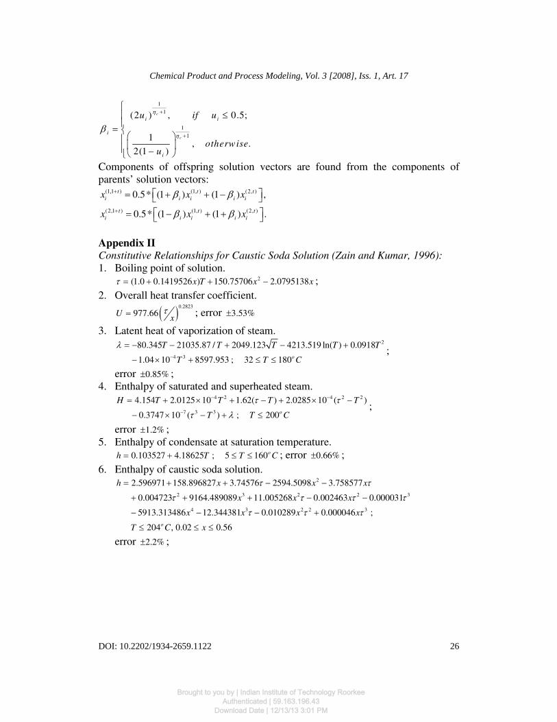
Appendix I

Offspring calculation in SBX crossover operator (Deb, 2001)

Spread factor i

β is calculated by generating random number (0,1)i

u ∈ as:

25

Danish et al.: Numerical Solution of Non-Linear Algebraic Equations

Brought to you by | Indian Institute of Technology RoorkeeAuthenticated | 59.163.196.43

Download Date | 12/13/13 3:01 PM

1

1

1

1

(2 ) , 0.5;

1, .

2(1 )

c

c

i i

i

i

u if u

otherwiseu

η

ηβ

+

+

≤

=

−

Components of offspring solution vectors are found from the components of

parents’ solution vectors: (1,1 ) (1, ) (2, )

(2,1 ) (1, ) (2, )

0.5* (1 ) (1 ) ,

0.5* (1 ) (1 ) .

t t t

i i i i i

t t t

i i i i i

x x x

x x x

β β

β β

+

+

= + + −

= − + +

Appendix II Constitutive Relationships for Caustic Soda Solution (Zain and Kumar, 1996):

1. Boiling point of solution. 2(1.0 0.1419526 ) 150.75706 2.0795138x T x xτ = + + − ;

2. Overall heat transfer coefficient.

( )0.2823

977.66Ux

τ= ; error 3.53%±

3. Latent heat of vaporization of steam. 2

4 3

80.345 21035.87 / 2049.123 4213.519 ln( ) 0.0918

1.04 10 8597.953 ; 32 180o

T T T T T

T T C

λ−

= − − + − +

− × + ≤ ≤;

error 0.85%± ;

4. Enthalpy of saturated and superheated steam. 4 2 4 2 2

7 3 3

4.154 2.0125 10 1.62( ) 2.0285 10 ( )

0.3747 10 ( ) ; 200o

H T T T T

T T C

τ τ

τ λ

− −

−

= + × + − + × −

− × − + ≤;

error 1.2%± ;

5. Enthalpy of condensate at saturation temperature.

0.103527 4.18625 ; 5 160oh T T C= + ≤ ≤ ; error 0.66%± ;

6. Enthalpy of caustic soda solution. 2

2 3 2 2 3

4 3 2 2 3

2.596971 158.896827 3.74576 2594.5098 3.758577

0.004723 9164.489089 11.005268 0.002463 0.000031

5913.313486 12.344381 0.010289 0.000046 ;

204 , 0.02 0.56o

h x x x

x x x

x x x x

T C x

τ τ

τ τ τ τ

τ τ τ

= + + − −

+ + + − −

− − − +

≤ ≤ ≤

error 2.2%± ;

26

Chemical Product and Process Modeling, Vol. 3 [2008], Iss. 1, Art. 17

DOI: 10.2202/1934-2659.1122

Brought to you by | Indian Institute of Technology RoorkeeAuthenticated | 59.163.196.43

Download Date | 12/13/13 3:01 PM

References

Androulakis, I.P., and Venkatasubramanian, V.A., Genetic algorithmic

framework for process design and optimization. Computers and Chemical

Engineering, (1991) 15(4), 217-228.

Angira, R. and Babu, B.V., Optimization of process synthesis and design

problems: A modified differential evolution approach. Chemical Engineering

Science, (2006) 61, 4707-4721.

Beigler, L.T., Grossmann, I.E., and Westerberg, A.W. (1997). Systematic methods

of chemical process design. New Jersey: Prentice Hall PTR.

Bhaskar, V., Gupta, S.K. and Ray, A.K., Applications of multiobjective

optimization in chemical engineering. Reviews in Chemical Engineering,

(2000a) 16, 1.

Bhaskar, V., Gupta, S.K. and Ray, A.K., Multiobjective optimization of an

industrial wiped film polyethylene terephthalate reactor. AIChE Journal,

(2000b) 46, 1046.

Bird, R. B., Stewart, W. E. and Lightfoot, E. N. (2002). Transport Phenomena.

Singapore: John Wiley & Sons (Asia) Pte. Ltd.

Coello Coello, C.A., Van Veldhuizen, D.A. and Lamont, G.B. (2002).

Evolutionary Algorithms For Solving Multi-Objective Problems. New York,

USA: Kluwer Academic/ Plenum Pub.

Costa, L., and Oliveira, P., Evolutionary algorithms approach to the solution of

mixed integer non-linear programming problems. Computers and Chemical

Engineering, (2001) 25, 257-266.

Danish M., Kumar S., Qamareen A., and Kumar S., “Optimal Solution of MINLP

Problems using Modified Genetic Algorithm”, Chemical Product and Process

Modeling (2006a), Volume 1, Issue 1, Article 4, pp. 1-41.

Danish M., Qamareen A., Kumar S. and Kumar S., Letter to the Editor,

Computers and Chemical Engineering (2006b) 31, 1364-1365.

Deb, K. (1995). Optimization for engineering design: algorithms and examples.

New Delhi, India: Prentice Hall.

Deb, K., An introduction to genetic algorithms. Sādhanā, (1999b) 24(4), 293-315.

Deb, K., Agrawal, S., Pratap, A. and Meyarivan, T., A fast and elitist non-

dominated sorting genetic algorithm for multi-objective optimization: NSGA-

II. In Proceedings of Parallel Problem Solving from Nature VI (PPSN-VI),

(2000a) pp. 849-858.

Deb, K. (2001). Multi-Objective Optimization using Evolutionary Algorithms.

Chichester, England: John Wiley & Sons Ltd.

Dennis, J.E. and Schnabel, R.B., (1983) Numerical Methods for Unconstrained

Optimization and Nonlinear Equations, Prentice-Hall Inc., Englewood Cliffs,

New Jersey.

27

Danish et al.: Numerical Solution of Non-Linear Algebraic Equations

Brought to you by | Indian Institute of Technology RoorkeeAuthenticated | 59.163.196.43

Download Date | 12/13/13 3:01 PM

Dorigo, M., Maniezzo, V., and Colorni, A., The ant system: Optimization by a

colony of cooperating agents. IEEE Transactions on Systems Man and

Cybernetics B, (1996) 26(2), 29-41.

Dorigo, M., and Stützle, T. (2005). Ant Colony Optimization. New Delhi, India:

Prentice Hall of India Pvt. Ltd.

Edgar, T.F., Himmelblau, D.M., and Lasdon, L.S. (2001). Optimization of

chemical processes. New York: McGraw-Hill.

Ferraris, G.B. and Tronconi, Enrico, BUNLSI- A FORTRAN Program for

Solution of Systems of Nonlinear Algebraic Equations. Computers and

Chemical Engineering, (1986) Vol. 10, No. 2, 129-141.

Floudas, C.A. (1995). Nonlinear and mixed-integer optimization. New York:

Oxford University.

Glover, F., Future paths for integer programming and links to artificial

intelligence. Comput. Oper. Res., (1986) 13, 533-549.

Goldberg, D.E. (1989). Genetic Algorithms in Search, Optimization, and Machine

Learning. Reading, MA: Addison-Wesley Pub. Co.

Grossmann, I.E., and Sargent, Roger W.H., Optimum Design of Multipurpose

Chemical Plants. Ind. Eng. Chem. Process Des. Dev., (1979) Vol.18, No.2,

343-348.

Gupta, S.K. (1995). Numerical Methods for Engineers. New Delhi: New Age

International Publishers Ltd.

Guria Chandan, Verma Mohan, Mehrotra, Surya P., and Gupta, S.K., Multi-

objective Optimal Synthesis and Design of Froth Floatation Circuits for

Mineral Processing, Using the Jumping Gene Adaptation of Genetic

Algorithm. Ind. Eng. Chem. Process Des. Dev., (2005) 44, 2621-2633.

Hansen, P. (1986). The steepest ascent mildest heuristic for combinatorial

programming. Congress on Numerical Methods in Combinatorial

Optimization, Capri, Italy.

Hilbert, R., Janiga, G., Baron, R., and Thévenin, D., Multi-objective shape

optimization of heat exchanger using parallel genetic algorithms. International

Journal of Heat and Mass Transfer, (2006) 49, 2567-2577.

Himmelblau, D.M. and Bischoff, K.B. (1968). Process Analysis and Simulation:

Deterministic Systems. New York: John Wiley & Sons, Inc.

Holland, J.H. (1975). Adaptation in natural and artificial systems. Ann Arbour:

University of Michigan Press.

Holland, C.D. (1975). Fundamentals and Modeling of Separation Processes.

Englewood Cliffs, New Jersey: Prentice-Hall Inc.

Kasat, Rahul B., and Gupta S.K., Multi-objective optimization of an industrial

fluidized-bed catalytic cracking unit (FCCU) using genetic algorithm (GA)

with the jumping genes operator. Computers and Chemical Engineering,

(2003) 27, 1785-1800.

28

Chemical Product and Process Modeling, Vol. 3 [2008], Iss. 1, Art. 17

DOI: 10.2202/1934-2659.1122

Brought to you by | Indian Institute of Technology RoorkeeAuthenticated | 59.163.196.43

Download Date | 12/13/13 3:01 PM

Kirkpatrick, S., Gelatt, C.D., and Vecchi, M.P., Optimization by simulated

annealing. Science, (1983) 220, 671-680.

Michalewicz, Z. (1992). Genetic algorithms + data structures = evolution

programs (2nd

Ed.). Berlin, Germany: Springer.

Mitchell, M. (1996). An Introduction to Genetic Algorithms. Cambridge, MA;

MIT Press.

Nandsana, A., Ray, A.K. and Gupta, S.K., Applications of non-dominated sorting

genetic algorithm in chemical engineering. International Journal of Chemical

Reactor Engineering, (2003) 1(R2), 1.

Reklaitis, G.V., Ravindran, A., and Ragsdell, K.M. (1983). Engineering

optimization methods and applications. New York: Wiley.

Sankararao, B. and Gupta, S.K., Modelling and simulation of fixed bed adsorbers

(FBAs) for multi-component gaseous separations. Computers and Chemical

Engineering, (2007a) 31, 1282-1295.

Sankararao, B., and Gupta S.K., Multi-objective optimization of an industrial

fluidized-bed catalytic cracking unit (FCCU) using two jumping gene

adaptations of simulated annealing. Computers and Chemical Engineering,

(2007b) 31, 1496-1515.

Shopova, E.G., and Natasha G. Vaklieva-Bancheva, BASIC-A genetic algorithm

for engineering problems solution. Computers and Chemical Engineering,

(2006) 30, 1293-1309.

Summanwar, V.S., Jayaram, V. K., Kulkarni, B. D., Kusumakar, H. S., Gupta, K.,

and Rajesh, J., Solution of constrained optimization problems by multi-

objective genetic algorithm. Computers and Chemical Engineering, (2002) 26,

1481-1492.

Tarafder, A., Rangaiah, G.P. and Ray, A.K., A study of finding many desirable

solutions in multiobjective optimization of chemical processes. Computers and

Chemical Engineering. (2007) 31, 1257-1271.

Upreti, S.R., and Deb, K., Optimal design of an ammonia synthesis reactor using

genetic algorithms. Computers and Chemical Engineering, (1997) 21(1), 87-

92.

Wodrich, M., and Bilchev, G., Cooperative distributed search: the ants’ way.

Control and Cybernetics, (1997) 26(3), 413-445.

Zain, O.S. and Kumar, S., “Simulation of Multiple Effect Evaporator for

Concentrating Caustic Soda Solution- Computational Aspects”, Journal of

Chemical Engineering of Japan (1996), Vol. 29, No. 5, pp. 889-893.

29

Danish et al.: Numerical Solution of Non-Linear Algebraic Equations

Brought to you by | Indian Institute of Technology RoorkeeAuthenticated | 59.163.196.43

Download Date | 12/13/13 3:01 PM