Simultaneous Quadrature Method of Moments for the Solution of PopulationBalance Equations, Using a Differential Algebraic Equation Framework

Jolius Gimbun,†,‡ Zoltan K. Nagy,*,† and Chris D. Rielly†

Department of Chemical Engineering, Loughborough UniVersity, Leicestershire, LE11 3TU, U.K., and Facultyof Chemical & Natural Resources Engineering, UniVersiti Malaysia Pahang, Lebuhraya Tun Razak,26300 Gambang, Pahang, Malaysia

The quadrature method of moments (QMOM) is a recent technique of solving population balance equationsfor particle dynamics simulation. In this paper, an alternative solution for the QMOM is described andthoroughly tested, which is based on the formulation and simultaneous solution of a semi-explicit differentialalgebraic equation (DAE) system. The DAE system consists of the ordinary differential equations resultingfrom the application of the method of moments, as well as a system of nonlinear algebraic equations derivedby applying the quadrature theory for the approximation of the moments. It is shown that the proposed approachprovides an efficient procedure for evolving the quadrature abscissas and weights from the QMOM. TheJacobian matrix of the DAE system is provided analytically to make the solution more robust. The DAE-QMOM method is compared to the well-established method for solving QMOM based on the product difference(PD) algorithm. The numerical results are compared to the analytical solutions in the case of breakage,aggregation, growth, and nucleation mechanisms. Excellent agreements are found on the moment evolutionpredicted by both methods. However, the DAE-QMOM method is found to be more accurate and robust thanthe PD-QMOM in some cases. Additionally, the DAE-QMOM is also capable of providing the solutionsignificantly faster than the PD-QMOM method.

1. Introduction

The population balance framework has been accepted forsome time as the most fundamental approach for modelingparticulate, droplet, or bubble dynamics in multiphase systems.A population balance is a powerful tool in evaluating the designof particulate related equipment such as crystallizers (e.g.,Randolph and Larson1), particularly when coupled with com-putational fluid dynamics (CFD) software.2-6 Many solutiontechniques have been developed to solve the population balanceequations, ranging from the simple standard method of moments(MOM), to the more advanced quadrature method of moments(QMOM), method of classes and direct numerical simulationapproaches such as high resolution finite volume7-9 and finiteelement schemes,10 or kinetic Monte Carlo techniques.11

The standard method of moments is one of the most commonmethods of solving population balance equations (PBEs). In theMOM, the PBE for a spatially homogeneous systems istransformed into a set of ordinary differential equations (ODEs)by multiplying the population balance equation by powers ofthe characteristics size (Lk) in a length based PBE and integratingit, giving equations in terms of the moments.1 For nonhomo-geneous systems, e.g., in the case of the CFD-PBM (populationbalance model), the MOM reduces the dimensionality of theproblem thus making the solution simpler. The MOM is knownto be an efficient method to solve the population balanceequation, but it suffers from a closure problem for casesinvolving size-dependent growth, coalescence, or aggregationprocesses. Therefore, the MOM is not directly applicable forgas-liquid systems, where bubble breakage and coalescenceare dominating mechanisms.

The method of characteristics (MOCh) is an alternativetechnique of solving the population balance equation as

demonstrated, e.g., by Lee et al.12 The MOCh for a first-orderpartial differential equation (PDE) determines the lines, calledcharacteristic lines, along which the PDE reduces to a set ofODEs. Once the ODEs are found, they can be solved easilyand transformed into a solution for the original PDE. The MOChhas the advantage of solving the PDE directly for the particlesize distribution with any required level of resolution along withthe moments; however, this method does not solve the closureproblem. Therefore, the MOCh cannot be directly applied tomodel systems involving breakage and coalescence, such as inthe case of gas-liquid dispersions.

Other classic solution techniques, such as the method ofclasses (MOC), are capable of solving the population balanceequation for growth, nucleation, breakage, coalescence, andaggregation processes. Although the terms “size class” or“sectional” had been used earlier by authors such as Gillette,13

Sutugin and Fuchs,14 Tolfo,15 and Gelbard et al.,16 the methodonly became readily available for implementation after a detailedderivation of the MOC for particle growth, breakage, andaggregation had been introduced by Marchal et al.17 The MOChas been applied to many problems involving breakage andcoalescence or aggregation processes for gas-liquid disper-sions,18,19 solid-liquid dispersions,20,21 and liquid-liquiddispersions.22-24 This method requires the whole particle sizedistribution (PSD) to be resolved into discrete size classes inorder to obtain an accurate solution. The number of discretizedequations increases with the number of size classes employed,and hence the solution for the MOC can be numericallyexpensive to obtain,25 especially for multiple coordinate systems,e.g., when coupled with three-dimensional CFD simulations.Most CFD-PBM studies26,27 only considered the Sauter meandiameter for calculations of the two-phase flow in CFD due tolimitation in computational resources. However, solution withmultiple particle/bubble size may become feasible in future asthe computational power continues to increase. Furthermore,the PBE solution obtained from MOC with a small number of

* To whom correspondence should be addressed. E-mail:z.k.nagy@lboro.ac.uk.

† Loughborough University.‡ Universiti Malaysia Pahang.

Ind. Eng. Chem. Res. 2009, 48, 7798–78127798

10.1021/ie900548s CCC: $40.75 2009 American Chemical SocietyPublished on Web 07/09/2009

Dow

nloa

ded

by U

NIV

MA

LA

YSI

A P

AH

AN

G o

n A

ugus

t 21,

200

9Pu

blis

hed

on J

uly

9, 2

009

on h

ttp://

pubs

.acs

.org

| do

i: 10

.102

1/ie

9005

48s

classes (e.g., Hounslow et al.21) introduces up to 5% error inthe moments prediction, which may affect prediction of theparticle size distribution.

McGraw28 proposed an attractive method for solving thepopulation balance equation, namely the quadrature method ofmoments (QMOM), which utilizes the quadrature theory toavoid the closure problem with standard MOM simulations. TheQMOM by McGraw28 is based on the product difference (PD)algorithm of Gordon.29 Application of the QMOM has beenextended into aggregation, coagulation, and breakage systemsby Wright et al.,30 Rosner and Pyykonen,31 Fan et al.,32 andMarchisio et al.33 However, the PD algorithm is not always thebest approach for computing the quadrature points from themoments of the particle size distribution (e.g., Lambin andGaspard34) because, for a larger number of moments, the methodis sensitive to small errors (e.g., Gautschi35). Therefore, theapplicability of QMOM is limited to no more than six quadraturepoints28 and even fewer for more complex cases such asdiffusion-controlled growth with secondary nucleation.

Later, McGraw and Wright36 proposed a new method, namelythe Jacobian matrix transformation (JMT) method, whichprovides an alternative approach to the PD algorithm. Thismethod is also based on the projection of the solution into thepower moments, yielding a set of equations for the evolutionof the quadrature rule. The JMT method, however, still suffersfrom the problem of ill conditioning, requiring the number ofmoments to be small.37 The occurrence of singularities in theQMOM with PD or JMT is the consequence of using the powermoments, thus making the calculation of population balanceunfeasible for a higher number of moments and hence a highernumber of quadrature points. Fan et al.32 proposed the directquadrature method of moments (DQMOM) as another alterna-tive to the PD algorithm. The DQMOM is based on the idea oftracking directly the variables appearing in the quadratureapproximation, by solving the convection equation for quadra-ture points and weights directly. The authors claim that someshortcomings of the PD-QMOM are avoided by solving theweights and abscissas directly especially when concerning aCFD-PBM problem. As Marchisio and Fox38 pointed out, theDQMOM can still be ill-conditioned for a higher number ofmoments because of the intrinsic problem of finding the rootsof high order polynomials.39 Su et al.40 suggested an improve-ment to DQMOM by introducing an adaptive factor in themoment equations which they claim to be able to improve theDQMOM accuracy for aggregation processes without adding asignificant computational expense (only 4% higher with theadaptive factor). The adaptive DQMOM does not increase theoriginal DQMOM accuracy for other systems such as growthand breakage, but it provides about 2% faster solution.

Recently, Alopaeus et al.41 proposed another solution, namelythe fixed quadrature method of moments (FQMOM). Thismethod exploits the zeros of orthogonal polynomials to findthe quadrature points. Unlike the PD-QMOM, which is restrictedto an even number of moments (twice the number of thequadrature points), the FQMOM can be applied to any numberof moments. The disadvantage of the FQMOM is that anoptimized arbitrary constant must be established before it canbe applied accurately for a specific problem. Finding thatoptimized constant might be easy for simple cases whereanalytical solution is available, but can be difficult for morecomplex systems.

Most of the currently available QMOM solutions are restrictedto using a small number of moments. Although a small numberof moments may be sufficient to describe the particulate

dynamics in simple cases, a larger number of moments mightbe required in other calculations, especially when an inversiontechnique is applied to discover the particle size distribution.Diemer and Ehrman,42 for example, needed at least 10 momentsto obtain acceptable reconstructions of the complete particle sizedistribution. Therefore, a better solution technique for thepopulation balance that is capable of solving for higher ordermoments is needed. This paper describes the possibility ofsolving the PBE via QMOM, without resorting to the PDalgorithm. An alternative solution technique for the QMOM isthoroughly tested, based on the simultaneous solution of themoment equations and quadrature approximation as a semi-explicit differential algebraic equation (DAE) system. A similarDAE based formulation of the QMOM was also studiedpreviously by Grosch et al.,43 although their work focusedmainly on crystallization systems with growth and nucleationmechanisms. The result from the DAE-QMOM method iscompared with the solution from the PD algorithm, as well asanalytical solutions, for various mechanisms including growth,nucleation, aggregation, and breakage.

2. Population Balance Equation

The dynamic population balance equation for a closedhomogeneous system can be written with diameter as the internalcoordinate as33,44

where �, a, G, B, b, L0, and δ are the aggregation kernel,breakage kernel, growth rate, nucleation rate, daughter particlesize distribution, size of the nuclei, and Dirac delta function,respectively, whereas both L and λ are the particle characteristiclength. The PBE in eq 1 can be further simplified using amoment transformation, where the kth moment of the distribu-tion, µk, is given by

The lower order moments (i.e., zeroth to third) are related tothe physical description of the particle size distribution; i.e., µ0

is related to the total number of particles, µ1 is related to thetotal particle diameter, µ2 is related to the total particle surfacearea, and µ3 is related to the total particle volume. After themoment transformation, the PBE of eq 1 is represented by aset of ODEs in terms of the moments:45

The moment equations represented by eq 3 are solvable forgrowth (but not size-dependent growth) and nucleation problemsusing the standard method of moment technique; however, it isnot possible to solve the breakage and coalescence terms dueto the closure problem, since the integrations cannot be writtenin term of the moments. Therefore, eq 3 needs to be transformed

µk ) ∫0

∞n(L)Lk dL (2)

Ind. Eng. Chem. Res., Vol. 48, No. 16, 2009 7799

Dow

nloa

ded

by U

NIV

MA

LA

YSI

A P

AH

AN

G o

n A

ugus

t 21,

200

9Pu

blis

hed

on J

uly

9, 2

009

on h

ttp://

pubs

.acs

.org

| do

i: 10

.102

1/ie

9005

48s

again into a quadrature method of moments formulation toeliminate the closure problem. The essence of the quadratureclosure is to consider the number density n(L) as a generalweight function and to approximate the integrals that appearduring the transformation of the PBE to moment equations interms of a set of abscissas and weights. The QMOM employsa quadrature approximation:28

where wi are the weights, Li are the abscissas, and N is thenumber of quadrature points. This quadrature approximation isexact if the function in eqs 4 are polynomials up to the order of2N - 1. After applying the quadrature rule, the momenttransformed PBE can be written as41

Now the closure problem has been eliminated, and hence thePBE in eq 5 is solvable by the means of the quadrature methodof moments by following the evolution of wi and Li, as well asµk. The moments are nonlinearly related to the weights andabscissas by eqs 4.

3. Numerical Techniques for QMOM

The QMOM calculations require integration of the ODEs eq5 for k ) 0, ... 2N - 1, alongside the nonlinear algebraic eqs 4.These equations may be numerically solved simultaneously asa set of coupled DAEs. However, most of the QMOM solutionsdescribed in the literature have been performed using the productdifference algorithm of Gordon28 to solve eqs 4. Solutions forthe population balance equation via the PD-QMOM are wellestablished for growth, nucleation, breakage, and aggregation/coalescence (e.g., McGraw;28 Marchisio et al.33). A variety ofalternative methods are available to solve the QMOM, includingFQMOM, JMT, and DQMOM (see section 1); however, thosetechniques are not widely used. Therefore, the solution fromthe DAE-QMOM is only compared with the most commontechnique for the QMOM, based on the PD algorithm.

3.1. DAE-QMOM. The DAE method is an attractive alterna-tive method for solving the QMOM since it arises from the naturalmathematical formulation of the QMOM approximation problemThe ODE eq 5 is generated from the moment equations, whereasthe algebraic eqs 4 are obtained from the quadrature rule. The DAE-QMOM method is illustrated in this section using a diffusion-controlled (size-dependent) growth model assuming the nucleation,breakage, and coalescence or aggregation rates are zero. In thediffusion-controlled growth model the growth rate is given by

where G0 is a constant. The population balance equation writtenin the form of the quadrature approximation is given by

For the case of N quadrature points, the DAE-QMOM methodrequires 2N moment ODEs and another 2N algebraic equationsfor the quadrature approximation. The first 2N moments aregenerated using eq 7, i.e.

The other 2N algebraic equations are generated using thequadrature approximation given by eqs 4.

Finally, the problem is represented by 4N equations containing4N unknowns made up from 2N moments, N weights, and Nabscissas. Equations 8 and 9 together represent a semi-explicitDAE system which can be solved using standard DAE solutiontechniques and software. In semi-explicit form the generic DAEcan be written as

where xb(t) contains the differential variables and zb(t) containsthe algebraic variables. The ODE eq 10 for xb(t) depends onadditional algebraic variables zb(t), and the solution is forced tosatisfy the algebraic constraints given by eq 11.46 In the caseof QMOM xb ) [µ0, µ1, ..., µ2N-1] and zb ) [w1, w2, ..., wN, L1,L2, ..., LN]. The semi-explicit system eqs 10 and 11 can bewritten as

where Mb is a mass matrix, and

and

The mass matrix for the DAE in eq 10 and 11 is given by

where I is the identity matrix of dimension nx × nx and nx isthe number of differential states. MATLAB is an efficientsoftware tool for numerical computation and can be used readilyfor the solution of index 1 DAE problems of the type shown ineq 12. The differential index of DAE is defined as the numberof differentiations needed to transform the DAE into an explicitODE. MATLAB can solve the DAE of index 1 via the ode15ssolver or ode23t solver.47 In this work, the ode15s solver isemployed to solve the DAE-QMOM. The ode15s is based on avariant of the backward differentiation formula (BDF) called

µk ) ∫0

∞n(L)Lk dL ≈ ∑

i)1

N

wiLik, for k ) 0, 1, 2 (4)

G(L) )G0

L(6)

dµk

dt) k ∑

i)1

N

G(Li(t))Li(t)k-1wi(t) (7)

dµ0

dt) 0

dµ1

dt)

G0

L1w1 +

G0

L2w2 + ... +

G0

LNwN

ldµ2N-1

dt) (2N - 1)

(8)

0 ) w1 + w2 + ... + wN - µ0

0 ) w1L1 + w2L2 + ... + wNLN - µ1

l0 ) w1L1

2N-1 + w2L22N-1 + ... + wNLN

2N-1 - µ2N-1

(9)

xf(t) ) f(xb, zb, t) (10)

0 ) g(xb, zb, t) (11)

Mb (t, yb)y ) Fb(t, yb) (12)

y ) (xz )

F ) (fg )

Mb ) (I 00 0 ) (13)

7800 Ind. Eng. Chem. Res., Vol. 48, No. 16, 2009

Dow

nloa

ded

by U

NIV

MA

LA

YSI

A P

AH

AN

G o

n A

ugus

t 21,

200

9Pu

blis

hed

on J

uly

9, 2

009

on h

ttp://

pubs

.acs

.org

| do

i: 10

.102

1/ie

9005

48s

the numerical differentiation formula (NDF).48 According toShampine and Reichelt,47 many tactics adopted for ode15sresemble those found in well-known codes such as LSODE49

and VODE.50 It was developed to integrate stiff ODEs andDAEs of the form of eq 12. The simplified Newton method isalso implemented in ode15s to perform a correction to thecurrent iteration (to satisfy the algebraic constraints), thussolving the DAE system. The requirement for the solution ofthe DAE system is the existence of a feasible initial conditionfor y0, that is, if there is a vector such that M(t0,y0)y ) F(t0,y0).The ode15s is implemented to detect automatically the DAEsystem and then to perform an automatic computation ofconsistent initial conditions for a robust computation. The DAEsystem might lead to instability of the solution, especially whena more complicated function is considered, e.g., involving thebreakage and coalescence kernels. To overcome such a problem,it is necessary to provide the analytical Jacobian matrix. TheJacobian of the DAE system is defined as follows:

where f1 to f2N are the right-hand sides (RHS) of the differentialmoment equations, f2N+1 to f4N are the RHS of the algebraicequations, y1 to y2N represent the moments, y2N+1 to y3N are theweights, and y3N+1 to y4N are the abscissas. The Jacobian matrixfor a given equation system can be generated using the symboliccomputation tool in MATLAB. If for example, for N ) 2, forthe diffusion-controlled growth only case, then the Jacobianmatrix, J, becomes

The Jacobian matrix can be divided into three major blocks.The first block, J(1,1) to J(2N,2N), contains the derivativesof the right-hand sides of the moment equations with respectto the moments. This particular block will remain unchanged,unless the RHS includes the moments. The second block,J(1,2N+1) to J(2N,4N), contains the derivatives of the RHS ofthe differential equations, with respect to the weights andabscissas. Therefore this block always changes whenever themechanism change. The third block, J(2N+1,1) to J(4N,4N), isderived from the algebraic equations of the quadrature ap-proximation and is the independent of the mechanisms used inthe PBE.

3.2. PD-QMOM. The solution of the QMOM via the PDalgorithm was first introduced by McGraw28 and has beenfurther developed for aggregation and breakage by Marchisioet al.33 The PD algorithm is employed to calculate the weightsand the abscissas from the moments in the QMOM. The firststep is the construction of a matrix P with components Pi,j

starting from the moments. The components in the first columnof matrix P are

where δi1 is the Kronecker delta. The components in the secondcolumn of P are

The remaining components can be computed from an iterativeequation as follows:

For example, when N ) 2, the matrix P becomes

The coefficients of the continued fraction (Ri) are generatedby setting the first element equal to zero (R1 ) 0) and computingthe others according to the following recursive relationship:

A symmetric tridiagonal matrix is then obtained from sumsand products of Ri:

and

where ai and bi are the diagonal and subdiagonal of the Jacobianmatrix. Once the tridiagonal matrix is determined, the abscissasand weights can be found by calculating the eigenvalues andeigenvectors of the tridiagonal matrix. The eigenvalues representthe abscissas, and the weights can be found from

where υj1 is the first component of the jth eigenvector. It shouldbe noted that the elements of the eigenvectors should benormalized such that the norm of each eigenvector is 1.0. Theeigenvalues and eigenvectors can be calculated numericallyusing the eig function in MATLAB.

4. Validation of the QMOM Algorithms

The performance of the DAE-QMOM is compared with thewell-established PD-QMOM method and with a number ofanalytical solutions. Six cases were tested, namely (i) diffusion-controlled growth (see section 3.1), (ii) constant growth andprimary nucleation, (iii) power-law growth, (iv) breakage, (v)constant aggregation kernel, and (vi) sum aggregation kernel.In each case, except for the power-law growth, the initial sizedistribution was

J ) [ ∂f1

∂y1

∂f1

∂y2· · ·

∂f1

∂y4N

∂f2

∂y1

∂f2

∂y2· · ·

∂f2

∂y4N

l l l l∂f4N

∂y1

∂f4N

∂y2· · ·

∂f4N

∂y4N

] (14)

Pi,1 ) δi1, i ) 1, ..., 2N + 1 (16)

Pi,2 ) (-1)i-1µi-1, i ) 1, ..., 2N + 1 (17)

Pi,j ) P1,j-1Pi+1,j-2 - P1,j-2Pi+1,j-1, j ) 3, ..., 2N +1 and i ) 1, ..., 2N + 2 - j (18)

P ) [1 µ0 µ1 µ2 - µ12 µ3µ1 - µ2

2

0 -µ1 -µ2 -µ3 + µ2µ1 00 µ2 µ3 0 00 -µ3 0 0 00 0 0 0 0

] (19)

Ri )P1,i+1

P1,iP1,i-1, i ) 2, ..., 2N (20)

ai ) R2i + R2i-1, i ) 1, ..., 2N - 1 (21)

bi ) -√R2i+1R2i-1, i ) 1, ..., 2N - 2 (22)

wj ) µ0υj12 (23)

n0(L) ) 3L2N0

V0e-L3/V0 (24)

Ind. Eng. Chem. Res., Vol. 48, No. 16, 2009 7801

Dow

nloa

ded

by U

NIV

MA

LA

YSI

A P

AH

AN

G o

n A

ugus

t 21,

200

9Pu

blis

hed

on J

uly

9, 2

009

on h

ttp://

pubs

.acs

.org

| do

i: 10

.102

1/ie

9005

48s

where N0 ) 1 m-3 and V0 ) 1 m3 or 0.001 m3. The particle sizedistribution in eq 24 is chosen because it has an analyticalsolution available from the literature. Unless otherwise stated,in ode15s the relative tolerance is set at 10-12 and the absolutetolerance is set at 10-10 for all cases tested in this work forboth the DAE-QMOM and the PD-QMOM. The relativetolerance (RelTol) represents the error that applies to allcomponents of the solution vector, whereas the absolutetolerance (AbsTol) applies to individual components of thesolution vector. The error in each integration step err(i) for anystate variable x(i) in the solution vectors satisfies the conditionerr(i) e max(RelTol · abs(x(i)),AbsTol(i)). A similar ODE/DAE

solver (ode15s) is employed for both the DAE-QMOM and thePD-QMOM. All solutions in this paper were computed usingthree quadrature points (six moments). The error of the predictedmoment is calculated as follows:

4.1. Growth and Nucleation Examples. Case 1: Diffusion-Controlled Growth. The moment equations for the diffusion-controlled growth have been described in section 3.1 (eqs 6-8).The initial distribution is given by eq 24 with N0 ) 1 m-3, V0

) 1 m3, and G0 ) 0.01 m2/s. The zeroth moment is the numberdensity of particles per unit volume and can be obtained byintegrating the initial distribution in eq 24 from zero to infinity.For the growth only case, µ0 will remain constant. Exactsolutions are available for zeroth and even moments only, givenby McGraw28 as

An analytical size distribution at any time t can be obtainedfrom41

Figure 1. Discontinuity of eq 29 at t ) 1 s. Upper right is the enlargedview of the discontinuity.

Figure 2. Error in the moment evolution for diffusion-controlled growth of DAE-QMOM (continuous lines) and PD-QMOM (circles).

% error )µanalytical - µcalculated

µanalytical× 100 (25)

µ0 ) N0 ) constant (26)

µ2 ) 2G0µ0t + µ2(0) (27)

µ4 ) 4G02µ0t

2 + 4G0µ2(0)t + µ4(0) (28)

7802 Ind. Eng. Chem. Res., Vol. 48, No. 16, 2009

Dow

nloa

ded

by U

NIV

MA

LA

YSI

A P

AH

AN

G o

n A

ugus

t 21,

200

9Pu

blis

hed

on J

uly

9, 2

009

on h

ttp://

pubs

.acs

.org

| do

i: 10

.102

1/ie

9005

48s

which then can be integrated numerically using the functionquadl in MATLAB to obtain the analytical solution for the oddmoments. An analytical integration is not possible for eq 29due to the presence of a discontinuity when L2 - 2G0t < 0.Figure 1 shows the plot of eq 29 at t ) 1 s. Equation 29 returnsan imaginary value at L < (2G0t)1/2, which results in adiscontinuity. A numerical integration via the quadl functionat a very small value of tolerance (function tolerance 10-12)was employed to calculate the odd moments. The lower limitof the quadl integration was set at L ) (2G0t)1/2, the point wherethe discontinuity starts.

The moments for the diffusion-controlled growth werepredicted remarkably well by both the DAE and PD methods,with a small error (mostly less than 10-8, see Figure 2) for thezeroth and even moments where the exact analytical solutionis available. There is no significant difference in the accuracyof the even moments predicted by the DAE-QMOM and PD-QMOM in this particular case, except for a very small differencein the fourth moment. The error for the odd moments issignificantly larger than that for the even moments, due to thefact that these are obtained from numerical integration of eq 29and not from the exact solution. Evolutions of the first sixmoments are shown in Figure 3; each moment is normalizedwith their initial value (µk(t)/µk(0)). In this case where onlygrowth is considered, the particle number density (zerothmoment) remains unchanged.

The DAE-QMOM and PD-QMOM were also tested to solvethe diffusion-controlled growth at a looser tolerance for ode15s(absolute tolerance ) relative tolerance ) 10-6) to furtherevaluate the robustness and accuracy of the proposed solution.Figure 4 shows the relative error of the moment evolution fromboth DAE-QMOM and PD-QMOM. For the case of a loosertolerance, prediction of the moment evolution by DAE-QMOMand PD-QMOM did not change much except for the fourthmoment, which was already showing some difference even forthe tight tolerance. The error in the fourth moment shows thatthe accuracy of moment prediction in this case depends onlyon the tolerance setting because the magnitude of errors reflectsthe absolute tolerance applied. Figure 5 shows the evolution ofthe weights from DAE-QMOM and PD-QMOM at the loosertolerance setting. For the case of the growth only problem, theweights should be constant because there is no change in theparticle number density. The individual weights are conservedperfectly by DAE-QMOM at looser tolerance; however, asignificant error is observed in the case of the PD-QMOMmethod.. There is no problem of conserving the weights at tighttolerance setting for both DAE-QMOM and PD-QMOM, andtherefore the results for weight evolution at tight tolerance arenot shown. Even for the looser tolerance, the total weights arewell conserved, even if the individual weights are not. In somecases when the individual weights are not conserved, some ofthe weights actually become zero and thus they no longercontribute to the PD solution. In such cases, the PD algorithmhas a singularity problem and is therefore no longer capable ofsolving the QMOM. The conservation of individual weights inQMOM is important to ensure that the solution is robust andaccurate. The weights are a crude approximation of the actualparticle size distribution. In the case of a normal distributionthe abscissa of the middle weight is similar to the mean diameterand the other two weights have a similar value (see Figure 6).The individual weights in the QMOM methods represent a

unique solution and therefore should be conserved perfectly inthe growth only problem. This numerical evaluation has clearlydemonstrated the robustness and accuracy of the DAE methodcompared to the PD algorithm in solving the population balanceequations.

Case 2: Constant Growth and Primary Nucleation. Thenext level of complication is to include nucleation, so thatthe number density of particle (µ0) increases with time. Theevolution of the zeroth moment for this case is given by

This particular case of constant growth rate, G, does notinvolve any closure problem and can be solved easily usingthe standard method of moments. The moments equation forthis case for MOM is given as follows:

where in this case study B0 ) 0.1 m-3s-1. The initial distributionis again given by eq 24 with N0 ) 1 m-3, V0 ) 1 m3, and G )0.01 m/s. The number of moments is not restricted for MOMand as many can be generated as are needed. A similar stiffODE solver, ode15s from MATLAB, was employed to solvethe MOM for a proper comparison with the QMOM method.Furthermore, the analytical solution for this case can be derivedeasily and the first three moments are given as follows:

The moment evolutions calculated using the two differentQMOM algorithms and the MOM are compared to the analyticalsolutions of eqs 32. Figure 7 shows very small errors in themoment evolutions calculated using the two different QMOMalgorithms and MOM. In this particular case the errors of thePD-QMOM and DAE-QMOM appear to be of similar magni-

n(L) )3N0

V0L√L2 - 2G0t exp(- (L2 - 2G0t)

3/2

V0) (29)

Figure 3. Moment evolution for diffusion-controlled growth from DAE-QMOM (circles) and analytical solution (continuous lines).

dµ0

dt) B0 (30)

dµ0

dt) B0

dµk

dt) kGµk-1, k g 1 (31)

µ0(t) ) B0t + µ0(0)µ1(t)

) GB0t2

2+ Gµ0(0)t + µ1(0)µ2(t)

) 2G2B0t3

3+ 2G2µ0(0)

t2

2+ 2Gµ1(0)t + µ2(0)

(32)

Ind. Eng. Chem. Res., Vol. 48, No. 16, 2009 7803

Dow

nloa

ded

by U

NIV

MA

LA

YSI

A P

AH

AN

G o

n A

ugus

t 21,

200

9Pu

blis

hed

on J

uly

9, 2

009

on h

ttp://

pubs

.acs

.org

| do

i: 10

.102

1/ie

9005

48s

tude. Prediction of the MOM was also found to be at an accuracysimilar to that for both QMOM solutions.

Case 3: Power-Law Growth. The power-law model iscommonly applied for crystallization growth and mass transferrelated problems. In the case evaluated in this work, a power-law growth model with the following relations without thenucleation term is considered.

where

and p ) 0.5 or -0.5. The case studied here is similar to thatevaluated by Alopaeus et al.51 However, the initial distributionis assumed to be a normal distribution with a mean size of Lj )0.5 m and a standard deviation σ ) 0.05 m instead of eq 24 inAlopaeus et al.’s51 work. An analytical size distribution at anytime t for this particular case of power-law growth is given by

where Lj and σ are the initial mean diameter and standarddeviation, respectively. A detailed derivation of the analytical

solution for power-law growth is given in the Appendix. Similarresults were reported by Alopaeus et al.51 for eq 24. The finalanalytical size distribution in eq 35 cannot be integratedanalytically to obtain the exact moments due to a discontinuityin the function. However, eq 35 can be integrated numericallyin MATLAB using the quadl solver to give an approximatevalue of the moments for comparison with the QMOM solution.The numerical integration employed a tight absolute toleranceof 10-12. The relative tolerance used in the ODE integrations isset to 10-12 for both cases (p ) 0.5 and p ) -0.5); however,it was necessary to reduce the absolute tolerance to 10-8 becausethe ODE integrator failed to solve the problem at a tightertolerance.

The comparison of relative errors in the moment evolutionsobtained using the DAE-QMOM and PD-QMOM methods forpower-law growth with p ) 0.5 and p ) -0.5 are presented inFigures 8 and 9, respectively. In both cases the DAE-QMOMdescribed the moment evolutions with a significantly lowerrelative error in most of the moments. For a negative value ofp, the smaller particles grow faster than the bigger ones causingthe particle size distribution to evolve as a shock wave,51

resulting in a major difficulty in conserving the individualweights (no nucleation in this case) generating the multiplicityproblem in the solution from the PD algorithm. Due to thissingularity problem the correct solution cannot be found evenfor a tighter tolerance (see Figure 10). As mentioned in thesection Case 1: Diffusion-Controlled Growth, the weights for a

Figure 4. Error of moment evolution for diffusion-controlled growth from DAE-QMOM (continuous lines) and PD-QMOM (circles) to the exact solution.

G(L) ) bLp (33)

b ) 0.81-p - 0.31-p

100(1 - p)(34)

n(L) ) 1

√2πσ(1 - (1 - p)bt

L1-p )p/(1-p)×

exp(- ((L1-p - (1 - p)bt)1/(1-p) - Lj)2

2σ2 ) (35)

7804 Ind. Eng. Chem. Res., Vol. 48, No. 16, 2009

Dow

nloa

ded

by U

NIV

MA

LA

YSI

A P

AH

AN

G o

n A

ugus

t 21,

200

9Pu

blis

hed

on J

uly

9, 2

009

on h

ttp://

pubs

.acs

.org

| do

i: 10

.102

1/ie

9005

48s

growth only problem should be perfectly conserved since thereis no change in the total number of particles in the system.

The tests on using loose (relative tolerance of 10-6 and absolutetolerance of 10-6) and tight (relative tolerance of 10-12 and absolutetolerance of 10-8) tolerance settings were carried out to assess therobustness of the new solution method. Figures 10 and 11 showthat the PD-QMOM fails to conserve the weights at tight toleranceand is even worse for the looser tolerance setting. In contrast, theDAE-QMOM conserves the weights at both looser and tighttolerance settings. For p ) -0.5 shown in Figure 10 the error inthe PD-QMOM solution becomes larger as time increases. Themoments are computed as a product between the weights andabscissas; thus any problem in predicting the weights could translate

into an error in the moment calculation. The moments may bepredicted fairly well even if the weights are not predicted correctlybecause the PD-QMOM counteracts the change in the weights byaltering the abscissas and forcing the moments to obey thequadrature rule. However, ill conditioning may occur when oneor more weights become zero, because they no longer contributeto the PD solution, and when this happens the PD-QMOM stopsproviding any solution. Thus it is important to obtain a correctprediction of the weights to maintain the robustness of the solutionprocess.

4.2. Aggregation Kernel Examples. The next stage ofcomplication is aggregation (coalescence), which leads tochanges in both the particle size distribution and the number

Figure 5. Evolution of weights at looser tolerance: DAE-QMOM (continu-ous lines) and PD-QMOM (dashed lines). Figure 6. Weights for normal distribution function for three quadrature

points (Lj ) 0.5 and σ ) 0.05).

Figure 7. Comparison of error for the first six moments for primary nucleation and constant growth of DAE-QMOM (continuous lines), PD-QMOM (circles),and MOM (triangles) compared with the analytical solution of eq 32.

Ind. Eng. Chem. Res., Vol. 48, No. 16, 2009 7805

Dow

nloa

ded

by U

NIV

MA

LA

YSI

A P

AH

AN

G o

n A

ugus

t 21,

200

9Pu

blis

hed

on J

uly

9, 2

009

on h

ttp://

pubs

.acs

.org

| do

i: 10

.102

1/ie

9005

48s

density of particles. Two different aggregation kernels weretested, namely the constant and sum kernel. The initial distribu-

tion employed for both aggregation kernels was given by eq24 with N0 ) 1 m-3 and V0 ) 0.001 m3.

Figure 8. Relative errors of the first six moments for power-law growth at p ) 0.5 of DAE-QMOM (continuous lines) and PD-QMOM (circles) to theanalytical solution.

Figure 9. Relative errors of the first six moments for power-law growth at p ) -0.5 of DAE-QMOM (continuous lines) and PD-QMOM (circles) comparedto the analytical solution.

7806 Ind. Eng. Chem. Res., Vol. 48, No. 16, 2009

Dow

nloa

ded

by U

NIV

MA

LA

YSI

A P

AH

AN

G o

n A

ugus

t 21,

200

9Pu

blis

hed

on J

uly

9, 2

009

on h

ttp://

pubs

.acs

.org

| do

i: 10

.102

1/ie

9005

48s

Case 4: Constant Aggregation Kernel. The constant ag-gregation kernel is given by

and in this case the breakage, growth, and nucleation terms areset to zero. The analytical solutions for the moments for thiscase can be obtained from the following equation:52

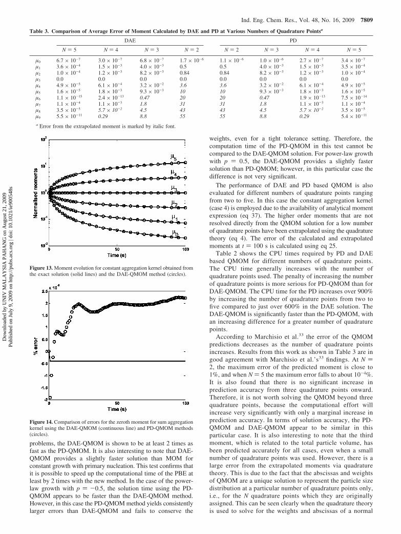
In Figure 12, the numerical solutions using the DAE-QMOMand PD-QMOM methods are compared to the analytical solutionfor the first six moments. In this case the errors of both DAE-QMOM and PD-QMOM are similar. The third moment whichis related to the total particle volume appears to be conservedvery well in this case, as shown in Figure 13. Each of themoments in Figure 13 are normalized with their initial value(µk(t)/µk(0)). For aggregation only problems, the zeroth moment(representing the number of bubble per unit volume) decreaseswith time. The first moment, which represents the total particlediameter, and the second moment, which is related to the totalparticle surface area, also decrease due to aggregation. The totalparticle volume is represented by the third moment. Forproblems involving only aggregation and/or breakage, the thirdmoment should be conserved, because there is no addition ofnew volume into the system. This is however not true forproblems involving growth and/or nucleation, where the totalvolume of particle is changing.

Case 5: Sum Aggregation Kernel. The sum aggregationkernel53,54 is given by

For this case the analytical solution is only available for thezeroth moment, which is given by

The third moment is also conserved in this case. Thepercentage error for the zeroth moment is significantly smallerin the case of the DAE-QMOM method than for the PD-QMOMas shown in Figure 14. Results from this example showed verylittle difference in prediction accuracy for both PD-QMOM andDAE-QMOM for aggregation kernel. Although there is a verysmall difference in the prediction for the zeroth moment, thedifference is negligible (less than 10-6) considering the errorfor other moments is larger than 10-3 (except for the µ3, whichis perfectly conserved).

4.3. Breakage Kernel. In this case the breakage kernel wasassumed to be proportional to the particle volume:

The uniform breakage function is assumed, which givesuniform probability of all fragment sizes:

Figure 10. Evolution of the weights for power-law growth at p ) -0.5 for DAE (continuous lines) and PD (dashed lines). (A) Looser tolerance (relativetolerance of 10-6 and absolute tolerance of 10-6); (B) tighter tolerance (relative tolerance of 10-12 and absolute tolerance of 10-8).

Figure 11. Evolution of the weights for power-law growth at p ) 0.5 for DAE (continuous line) and PD (dashed line). (A) Looser tolerance (relativetolerance of 10-6 and absolute tolerance of 10-6); (B) tighter tolerance (relative tolerance of 10-12 and absolute tolerance of 10-8).

�(L, λ) ) 1 (36)

µk ) µk0( 22 + N0�(L, λ)t)1-((k-1)/3)

(37)

�(L, λ) ) L3 + λ3 (38)

µ0 ) N0e-N0V0t (39)

g(L) ) L3 (40)

b(L, λ) ) 6L2

λ3(41)

Ind. Eng. Chem. Res., Vol. 48, No. 16, 2009 7807

Dow

nloa

ded

by U

NIV

MA

LA

YSI

A P

AH

AN

G o

n A

ugus

t 21,

200

9Pu

blis

hed

on J

uly

9, 2

009

on h

ttp://

pubs

.acs

.org

| do

i: 10

.102

1/ie

9005

48s

The daughter particle distribution function, b(L,λ), determinesthe number and size of the daughter particle, L, after thebreakage event of particle size λ. For the uniform breakagefunction, binary breakage with similar particle sizes is assumed.

In this case the aggregation, growth, and nucleation termsare set to zero. The initial particle distribution is given by eq24 with N0 ) 1 m-3 and V0 ) 1 m3. In this case the analyticalsolution at any time t is given by (e.g., Hounslow et al.21)

which then can be integrated analytically using the int functionin MATLAB to obtain the exact moments. The analyticalintegration was performed with the limits from zero to infinity.As shown in Figure 15, the errors from both the DAE-QMOM

and PD-QMOM in this case are small, on the order of ∼0.1%or less, and similar. The third moment is also well conserved,as shown in Figure 16. The profiles for the evolution of thenormalized moments for the breakage kernel (Figure 16) arethe reverse of those for the aggregation kernel in Figure 13.For this breakage only problem, the first three moments increasesteadily as the large particles break into smaller particles. It isclear from the test for breakage only that both the DAE-QMOMand PD-QMOM methods yielded similar accuracy.

5. Comparison of Computational Effort for PD-QMOMand DAE-QMOM

Apart from the prediction accuracy, the performance of theDAE-QMOM, in terms of CPU times is also compared to thatof the existing PD-QMOM method. The test was carried outby employing a similar ODE solver (ode15s) and tolerance(similar to those applied for cases 1-6) for both PD and DAEalgorithms. The comparison of the CPU times for the variousPBE solutions is shown in Table 1. DAE-QMOM is more than3 times faster than the existing solution via PD-QMOM forconstant aggregation and growth with the primary nucleationproblems. For the breakage and diffusion-controlled growth

Figure 12. Comparison of errors for the first six moments for constant aggregation kernel using DAE-QMOM (continuous lines) and PD-QMOM (circles)compared to the analytical solution of eqs 4-37.

Table 1. Comparison of the CPU Time in seconds for Different Solution Methods for the Population Balance Equation

power-law growth

PBE solutiondiffusion-controlled

growthconstant growth

and primary nucleation p ) 0.5 p ) -0.5 aggregationa breakageb

DAE 0.781 0.516 0.406 1.630 0.609 1.875PD 1.375 1.703 0.435 fails 3.188 3.547MOM 0.562

a Constant. b Proportional to volume.

Table 2. Comparison of CPU Time of DAE and PD at VariousNumber of Quadrature Points (CPU Speed 3.8 GHz, MATLAB2006a)

N

2 3 4 5

tDAE (s) 0.38 0.49 1.21 2.81tPD (s) 1.72 4.74 8.15 18.26

n(L) ) 3L2(1 + t)2e-L3(1+t) (42)

7808 Ind. Eng. Chem. Res., Vol. 48, No. 16, 2009

Dow

nloa

ded

by U

NIV

MA

LA

YSI

A P

AH

AN

G o

n A

ugus

t 21,

200

9Pu

blis

hed

on J

uly

9, 2

009

on h

ttp://

pubs

.acs

.org

| do

i: 10

.102

1/ie

9005

48s

problems, the DAE-QMOM is shown to be at least 2 times asfast as the PD-QMOM. It is also interesting to note that DAE-QMOM provides a slightly faster solution than MOM forconstant growth with primary nucleation. This test confirms thatit is possible to speed up the computational time of the PBE atleast by 2 times with the new method. In the case of the power-law growth with p ) -0.5, the solution time using the PD-QMOM appears to be faster than the DAE-QMOM method.However, in this case the PD-QMOM method yields consistentlylarger errors than DAE-QMOM and fails to conserve the

weights, even for a tight tolerance setting. Therefore, thecomputation time of the PD-QMOM in this test cannot becompared to the DAE-QMOM solution. For power-law growthwith p ) 0.5, the DAE-QMOM provides a slightly fastersolution than PD-QMOM; however, in this particular case thedifference is not very significant.

The performance of DAE and PD based QMOM is alsoevaluated for different numbers of quadrature points rangingfrom two to five. In this case the constant aggregation kernel(case 4) is employed due to the availability of analytical momentexpression (eq 37). The higher order moments that are notresolved directly from the QMOM solution for a low numberof quadrature points have been extrapolated using the quadraturetheory (eq 4). The error of the calculated and extrapolatedmoments at t ) 100 s is calculated using eq 25.

Table 2 shows the CPU times required by PD and DAEbased QMOM for different numbers of quadrature points.The CPU time generally increases with the number ofquadrature points used. The penalty of increasing the numberof quadrature points is more serious for PD-QMOM than forDAE-QMOM. The CPU time for the PD increases over 900%by increasing the number of quadrature points from two tofive compared to just over 600% in the DAE solution. TheDAE-QMOM is significantly faster than the PD-QMOM, withan increasing difference for a greater number of quadraturepoints.

According to Marchisio et al.33 the error of the QMOMpredictions decreases as the number of quadrature pointsincreases. Results from this work as shown in Table 3 are ingood agreement with Marchisio et al.’s33 findings. At N )2, the maximum error of the predicted moment is close to1%, and when N ) 5 the maximum error falls to about 10-4%.It is also found that there is no significant increase inprediction accuracy from three quadrature points onward.Therefore, it is not worth solving the QMOM beyond threequadrature points, because the computational effort willincrease very significantly with only a marginal increase inprediction accuracy. In terms of solution accuracy, the PD-QMOM and DAE-QMOM appear to be similar in thisparticular case. It is also interesting to note that the thirdmoment, which is related to the total particle volume, hasbeen predicted accurately for all cases, even when a smallnumber of quadrature points was used. However, there is alarge error from the extrapolated moments via quadraturetheory. This is due to the fact that the abscissas and weightsof QMOM are a unique solution to represent the particle sizedistribution at a particular number of quadrature points only,i.e., for the N quadrature points which they are originallyassigned. This can be seen clearly when the quadrature theoryis used to solve for the weights and abscissas of a normal

Table 3. Comparison of Average Error of Moment Calculated by DAE and PD at Various Numbers of Quadrature Pointsa

DAE PD

N ) 5 N ) 4 N ) 3 N ) 2 N ) 2 N ) 3 N ) 4 N ) 5

µ0 6.7 × 10-7 3.0 × 10-7 6.8 × 10-7 1.7 × 10-6 1.1 × 10-6 1.0 × 10-6 2.7 × 10-7 3.4 × 10-7

µ1 3.6 × 10-4 1.5 × 10-3 4.0 × 10-3 0.5 0.5 4.0 × 10-3 1.5 × 10-3 3.5 × 10-4

µ2 1.0 × 10-4 1.2 × 10-3 8.2 × 10-3 0.84 0.84 8.2 × 10-3 1.2 × 10-3 1.0 × 10-4

µ3 0.0 0.0 0.0 0.0 0.0 0.0 0.0 0.0µ4 4.9 × 10-5 6.1 × 10-4 3.2 × 10-2 3.6 3.6 3.2 × 10-2 6.1 × 10-4 4.9 × 10-5

µ5 1.6 × 10-5 1.8 × 10-3 9.3 × 10-3 10 10 9.3 × 10-3 1.8 × 10-3 1.6 × 10-5

µ6 1.1 × 10-15 2.4 × 10-13 0.47 20 20 0.47 1.9 × 10-13 7.5 × 10-14

µ7 1.1 × 10-4 1.1 × 10-3 1.8 31 31 1.8 1.1 × 10-3 1.1 × 10-4

µ8 3.5 × 10-5 5.7 × 10-2 4.5 43 43 4.5 5.7 × 10-2 3.5 × 10-5

µ9 5.5 × 10-11 0.29 8.8 55 55 8.8 0.29 5.4 × 10-11

a Error from the extrapolated moment is marked by italic font.

Figure 13. Moment evolution for constant aggregation kernel obtained fromthe exact solution (solid lines) and the DAE-QMOM method (circles).

Figure 14. Comparison of errors for the zeroth moment for sum aggregationkernel using the DAE-QMOM (continuous line) and PD-QMOM methods(circles).

Ind. Eng. Chem. Res., Vol. 48, No. 16, 2009 7809

Dow

nloa

ded

by U

NIV

MA

LA

YSI

A P

AH

AN

G o

n A

ugus

t 21,

200

9Pu

blis

hed

on J

uly

9, 2

009

on h

ttp://

pubs

.acs

.org

| do

i: 10

.102

1/ie

9005

48s

distribution function. For N ) 2, two abscissas of similarweights are produced, while at N ) 3, one abscissa of largerweights is placed exactly at Lmean and the other two on theleft and right have the same weight, significantly lower thanthe weights for Lmean. Thus a significant error is present whenthe weights and abscissas obtained from N ) 2 are employedto extrapolate the higher order moments, i.e., fourth and fifth,because the abscissas and weights for N ) 2 are no longera unique solution for N ) 3.

6. Conclusions

A new QMOM method for solving the population balanceequation has been proposed, which solves simultaneously thedifferential equations for the moments and the system ofnonlinear equations resulting from the quadrature approximationas a differential algebraic equation system. The solutions fromthe proposed method are compared to the product differencebased QMOM. Both methods have been validated against theanalytical solutions for growth, nucleation, breakage, andcoalescence. The results indicate that both methods are capableof predicting accurately the moment evolutions in all cases testedin this study, except for one case of power-law growth. Thenew numerical solution for the QMOM via DAE method hasbeen demonstrated to be more robust and accurate than the PDalgorithm in some cases, especially for growth only problems,characteristic of a large number of applications in particular inthe field of crystallization. The DAE-QMOM did not improvethe PD-QMOM predictions for the breakage and aggregationkernels evaluated in this work; however, there is a measurableimprovement observed for the sum aggregation case. The DAE-QMOM has a mathematically simpler formulation eliminatingthe additional complexity related to the product differencealgorithm, providing a more robust solution framework. Theonly downside of the DAE-QMOM at present is the lack of anautomatic Jacobian generator in the DAE solver. At present theJacobian elements are computed symbolically in software suchas MATLAB or MAPLE and then included manually withinthe DAE-QMOM algorithm. However, the use of DAE solverswith automatic differentiation would make the DAE-QMOMmuch simpler to implement than the PD-QMOM. Apart from

Figure 15. Comparison of error for the first six moments for proportional to volume breakage kernel obtained using the DAE-QMOM method (continuouslines) and PD-QMOM method (circles).

Figure 16. Moment evolution for proportional to volume breakage kernelusing the DAE-QMOM method (solid lines) and the exact solution (circles).

7810 Ind. Eng. Chem. Res., Vol. 48, No. 16, 2009

Dow

nloa

ded

by U

NIV

MA

LA

YSI

A P

AH

AN

G o

n A

ugus

t 21,

200

9Pu

blis

hed

on J

uly

9, 2

009

on h

ttp://

pubs

.acs

.org

| do

i: 10

.102

1/ie

9005

48s

being able to provide a more accurate solution, the DAE-QMOMalso provides a faster solution than both PD-QMOM and MOMfor all cases evaluated in this work, assessed from the CPUtimes required to perform the calculation, which is a significantadvantage of the method especially when the PBE has to besolved in the context of CFD simulations.

Acknowledgment

J.G. is grateful to the scholarship from Ministry of HigherEducation, Malaysia, and Universiti Malaysia Pahang.

Appendix: Derivation of Analytical Solution forPower-Law Growth

PBE for the growth only problem is given by

The growth law is given by

After differentiation, the growth law is

Replacing eq A.4 into eq A.2:

From the method of characteristics, the characteristic linesin which the PDE reduces to ODEs can be represented asfollows:

Applying the chain rule

Comparing eq A.7 to A.5 results in

Since t - t0 ) s - s0 assuming t0 ) s0 ) 0, thus t ) s.Equations A.8 become

Integrating eq A.9 with respect to L and t:

Integrating eq A.10:

After rearranging

Replace L0 with eq A.13:

When the initial distribution is a normal distribution givenby

The final distribution at any time t is given by

Literature Cited

(1) Randolph, A. D.; Larson, M. A. Theory of particulate processes:Analysis and techniques of continuous crystallization; Academic Press: NewYork, 1971.

(2) Gerstlauer, A.; Motz, S.; Mitrovic, A.; Gilles, E. Development,analysis and validation of population models for continuous and batchcrystallizers. Chem. Eng. Sci. 2002, 57 (20), 4311–4327.

(3) Jaworski, Z.; Nienow, A. W. CFD modelling of continuous precipita-tion of barium sulphate in a stirred tank. Chem. Eng. J. 2003, 91, 167–174.

(4) Wei, H.; Zhou, W.; Garside, J. Computational fluid dynamicsmodeling of the precipitation process in a semibatch crystallizer. Ind. Eng.Chem. Res. 2001, 40, 5255–5261.

(5) Woo, X. Y.; Tan, R. B. H.; Chow, P. S.; Braatz, R. D. Simulationof mixing effects in antisolvent crystallization using a coupled CFD-PDF-PBE approach. Cryst. Growth Des. 2006, 6, 1291–1303.

(6) Woo, X. Y.; Tan, R. B. H.; Braatz, R. D. Modeling and computationalfluid dynamics-population balance equation-micromixing simulation ofimpinging jet crystallizers. Cryst. Growth Des. 2009, 9, 156–164.

∂n∂t

+ ∂(Gn)∂L

) 0 (A.1)

∂n∂t

+ G∂n∂L

+ n∂G∂L

) 0 (A.2)

G ) bLp (A.3)

∂G∂L

) bpLp-1 (A.4)

∂n∂t

+ G∂n∂L

) -nbpLp-1 (A.5)

n(L, t) ) n(L(s), t(s)) (A.6)

∂n∂s

) dLds

∂n∂L

+ dtds

∂n∂L

(A.7)

dtds

) 1dLds

) Gdnds

) -nbpLp-1 (A.8)

dLdt

) bLp (A.9)

dndt

) -nbpLp-1 (A.10)

∫L0

L dL

Lp) b∫0

tdt; [( 1

1 - p)L1-p]L0

L) bt (A.11)

L ) (L01-p + (1 - p)bt)1/(1-p) (A.12)

L0 ) (L1-p - (1 - p)bt)1/(1-p) (A.13)

∫n0

n dnn

) -bp∫0

tLp-1 dt (A.14)

lnnn0

) -bp∫0

t 1

L01-p + (1 - p)bt

dt

) [-bp1

(1 - p)bln(L0

1-p + (1 - p)bt)]0

t

) pp - 1

ln(L01-p + (1 - p)bt

L01-p )

) ln(1 + (1 - p)bt

L01-p )p/(p-1)

(A.15)

n ) n0(1 + (1 - p)bt

L01-p )p/(p-1)

(A.16)

n ) n0(L0)(1 + (1 - p)bt

L1-p - (1 - p)bt)p/(p-1)

) n0(L0)(L1-p - (1 - p)bt + (1 - p)bt

L1-p - (1 - p)bt )p/(p-1)

) n0(L0)(L1-p - (1 - p)bt

L1-p )p/(1-p)

) n0(L0)(1 - (1 - p)bt

L1-p )p/(1-p)(A.17)

n0(L) ) 1

σ√2πexp(- (L - Lj)2

2σ2 ) (A.18)

n(L) ) 1

σ√2πexp(- ((L1-p + (1 - p)bt)1/(1-p) - Lj)2

2σ2 ) ×

(1 - (1 - p)bt

L1-p )p/(1-p)(A.19)

Ind. Eng. Chem. Res., Vol. 48, No. 16, 2009 7811

Dow

nloa

ded

by U

NIV

MA

LA

YSI

A P

AH

AN

G o

n A

ugus

t 21,

200

9Pu

blis

hed

on J

uly

9, 2

009

on h

ttp://

pubs

.acs

.org

| do

i: 10

.102

1/ie

9005

48s

(7) Gunawan, R.; Fusman, I.; Braatz, R. D. High resolution finite volumemethods for simulating multidimensional population balance equations withnucleation and size dependent growth. AIChE J. 2004, 50, 2738–2749.

(8) Gunawan, R.; Fusman, I.; Braatz, R. D. Parallel high resolutionsimulation of particulate processes with nucleation, growth, and aggregation.AIChE J. 2008, 54, 1449–1458.

(9) Zhang, T.; Tade, M. O.; Tian, Y. C.; Zang, H. High-resolutionmethod for numerically solving PDEs in process engineering. Comput.Chem. Eng. 2008, 32, 2403–2408.

(10) Ulbert, Z.; Lakatos, B. G. Dynamic simulation of crystallizationprocesses: Adaptive finite element collocation method. AIChE J. 2007, 53,3089–3107.

(11) Rosner, D. E.; McGraw, R. L.; Tandon, P. Multi-variate populationbalances via moment- and Monte Carlo simulation methods. Ind. Eng. Chem.Res. 2003, 42, 2699–2711.

(12) Lee, K.; Lee, J. H.; Yang, D. R.; Mahoney, A. W. Integrated run-to-run and on-line model-based control of particle size distribution for asemi-batch precipitation reactor. Comput. Chem. Eng. 2002, 26, 1117–1131.

(13) Gillette, D. A. A study of aging of lead aerosolssII: A numericalmodel simulating coagulation and sedimentation of a leaded aerosol in thepresence of an unleaded background aerosol. Atmos. EnViron. 1970, 6, 451–462.

(14) Sutugin, A. G.; Fuchs, N. A. Formation of condensation aerosolsunder rapidly changing environmental conditions. Theory and method ofcalculation. J. Aerosol Sci. 1970, 1, 287–293.

(15) Tolfo, F. A simplified model of aerosol coagulation. J. AerosolSci. 1977, 8, 9–19.

(16) Gelbard, F.; Tambour, Y.; Seinfeld, J. H. Sectional representationsfor simulating aerosol dynamics. J. Colloid Interface Sci. 1980, 76, 541–556.

(17) Marchal, P.; David, R.; Klein, J. P.; Villermaux, J. Crystallizationand precipitation engineeringsI: An efficient method for solving populationbalance in crystallization with agglomeration. Chem. Eng. Sci. 1988, 43,59–67.

(18) Chen, P.; Sanyal, J.; Dudukovic, M. P. CFD modeling of bubblecolumns flows: Implementation of population balance. Chem. Eng. Sci. 2004,59, 5201–5207.

(19) Dhanasekharan, K. M.; Sanyal, J.; Jain, A.; Haidari, A. Ageneralized approach to model oxygen transfer in bioreactors usingpopulation balances and computational fluid dynamics. Chem. Eng. Sci.2005, 60, 213–218.

(20) Kumar, S.; Ramkrishna, D. On the solution of population balanceequations by discretizationsIII. Nucleation, growth and aggregation ofparticles. Chem. Eng. Sci. 1997, 52, 4659–4679.

(21) Hounslow, M. J.; Pearson, J. M. K.; Instone, T. Tracer studies ofhigh-shear granulation: II. Population balance modeling. AIChE J. 2001,47, 1984–1999.

(22) Chen, Z.; Pruss, J.; Warnecke, H.-J. A population balance modelfor disperse systems: Drop size distribution in emulsion. Chem. Eng. Sci.1998, 53, 1059–1066.

(23) Alopaeus, V.; Koskinen, J.; Keskinen, K. I. Utilization of populationbalances in simulation of liquid-liquid systems in mixed tanks. Chem. Eng.Commun. 2003, 190, 1468–1484.

(24) Floury, J.; Legrand, J.; Desrumaux, A. Analysis of a new type ofhigh pressure homogeniser. Part B. study of droplet break-up and recoa-lescence phenomena. Chem. Eng. Sci. 2004, 59, 1285–1294.

(25) Costa, C. B. B.; Maciel, M. R. W.; Filho, R. M. Considerations onthe crystallization modeling: Population balance solution. Comput. Chem.Eng. 2007, 31, 206–218.

(26) Gimbun, J.; Rielly, C. D.; Nagy, Z. K. Modelling of mass transferin gas-liquid stirred tanks agitated by Rushton turbine and CD-6 impeller:A scale-up study. Chem. Eng. Res. Des. 2009, 87, 437–451.

(27) Moilanen, P.; Laakkonen, M.; Visuri, O.; Alopaeus, V.; Aittamaa,J. Modelling mass transfer in an aerated 0.2 m3 vessel agitated by Rushton,Phasejet and Combijet impellers. Chem. Eng. J. 2008, 142, 95–108.

(28) McGraw, R. Description of aerosol dynamics by the quadraturemethod of moments. Aerosol Sci. Technol. 1997, 27, 255–265.

(29) Gordon, R. G. Error bounds in equilibirium statistical mechanics.J. Math. Phys. 1968, 9, 655–663.

(30) Wright, D. L.; McGraw, R.; Rosner, D. E. Bivariate extension ofthe quadrature method of moments for modeling simultaneous coagulationand sintering of particle populations. J. Colloid Interface Sci. 2001, 236,242–251.

(31) Rosner, D. E.; Pyykonen, J. J. Bivariate moment simulation ofcoagulating and sintering nanoparticles in flames. AIChE J. 2002, 48, 476–491.

(32) Fan, R.; Marchisio, D. L.; Fox, R. O. Application of the directquadrature method of moments to polydisperse gas-solid fluidized beds.Powder Technol. 2004, 139, 7–20.

(33) Marchisio, D. L.; Vigil, R. D.; Fox, R. O. Quadrature method ofmoments for aggregation-breakage processes. J. Colloid Interface Sci. 2003,258, 322–334.

(34) Lambin, P.; Gaspard, J. P. Continued-fraction technique for tight-binding systems. A generalized-moments method. Phys. ReV. B 1982, 26,4356–4368.

(35) Gautschi, W. Algorithm 726: ORTHPOL-a package of routines forgenerating orthogonal polynomials and Gauss-type quadrature rules. ACMTrans. Math. Software 1994, 20, 21–62.

(36) McGraw, R.; Wright, D. L. Chemically resolved aerosol dynamicsfor internal mixtures by the quadrature method of moments. J. Aerosol Sci.2003, 34, 189–209.

(37) Dorao, C. A.; Jakobsen, H. A. The quadrature method of momentsand its relationship with the method of weighted residuals. Chem. Eng.Sci. 2006, 61, 7795–7804.

(38) Marchisio, D. L.; Fox, R. O. Solution of population balanceequations using the direct quadrature method of moments. J. Aerosol Sci.2005, 36, 43–73.

(39) Press, W. H.; Flannery, B. P.; Teukolsky, S. A.; Vetterling, W. T.Numerical Recipes in C: The Art of Scientific Computing, 2nd ed.;Cambridge University Press: Cambridge, 1992.

(40) Su, J.; Gu, Z.; Li, Y.; Feng, S.; Xu, X. Y. An adaptive directquadrature method of moment for population balance equations. AIChE J.2008, 54, 2872–2887.

(41) Alopaeus, V.; Laakkonen, M.; Aittamaa, J. Numerical solution ofmoment-transformed population balance equation with fixed quadraturepoints. Chem. Eng. Sci. 2006, 61, 4919–4929.

(42) Diemer, R. B.; Ehrman, S. H. Pipeline agglomerator design as amodel test case. Powder Technol. 2005, 156, 129–145.

(43) Grosch, R.; Briesen, H.; Marquardt, W.; Wulkow, M. Generalizationand numerical investigation of QMOM. AIChE J. 2007, 53, 207–227.

(44) Rod, V.; Misek, T. Stochastic modelling of dispersion formationin agitated liquid-liquid systems. Trans. Inst. Chem. Eng. 1982, 60, 48–53.

(45) Hulburt, H. M.; Katz, S. Some problems in particle technology.Chem. Eng. Sci. 1964, 19, 555–574.

(46) Ascher, U. M.; Petzold, L. R. Computer Methods for OrdinaryDifferential Equations and Differential Algebraic Equations, 1st ed.; Societyfor Industrial and Applied Mathematics: Philadelphia, PA, 1998.

(47) Shampine, L. F.; Reichelt, M. W. MATLAB ODE suite. SIAM J.Sci. Comput. 1997, 18, 1–22.

(48) Klopfenstein, R. W. Numerical differentiation formulas for stiffsystems of ordinary differential equations. RCA ReV. 1971, 32, 447–462.

(49) Hindmarsh, A. C. LSODE and LSODI, two new initial valueordinary differential equation solvers. ACM SIGNUM Newslett. 1980, 15,10–11.

(50) Brown, P. N.; Byrne, G. D.; Hindmarsh, A. C. VODE: A variable-coefficient ODE solver. SIAM J. Sci. Comput. 1989, 10, 1038–1051.

(51) Alopaeus, V.; Laakkonen, M.; Aittamaa, J. Solution of populationbalances with growth and nucleation by high order moment-conservingmethod of classes. Chem. Eng. Sci. 2007, 62, 2277–2289.

(52) Gelbard, F.; Seinfeld, J. H. Numerical solution of the dynamicequation for particulate systems. J. Comput. Phys. 1978, 28, 357–375.

(53) Melzak, Z. A. The effects of coalescence in certain collisionprocesses. Q. J. Appl. Math. 1953, 11, 231.

(54) Scott, W. T. Analytic studies on cloud droplet coalescence. J. Atmos.Sci. 1968, 25, 54.

ReceiVed for reView April 3, 2009ReVised manuscript receiVed June 16, 2009

Accepted June 21, 2009

IE900548S

7812 Ind. Eng. Chem. Res., Vol. 48, No. 16, 2009

Dow

nloa

ded

by U

NIV

MA

LA

YSI

A P

AH

AN

G o

n A

ugus

t 21,

200

9Pu

blis

hed

on J

uly

9, 2

009

on h

ttp://

pubs

.acs

.org

| do

i: 10

.102

1/ie

9005

48s