How Floquet Theory Applies to Index 1 Differential Algebraic Equations
23
Ž . JOURNAL OF MATHEMATICAL ANALYSIS AND APPLICATIONS 217, 372]394 1998 ARTICLE NO. AY975714 How Floquet Theory Applies to Index 1 Differential Algebraic Equations Rene Lamour, Roswitha Marz, and Renate Winkler ´ ¨ Institut fur Mathematik, Humboldt-Uni ¤ ersitat zu Berlin, 10099 Berlin, Germany ¨ ¨ Submitted by Robert O’Malley Received July 1, 1996 Local stability of periodic solutions is established by means of a Floquet theory for index-1 differential algebraic equations. Linear differential algebraic equations with periodic coefficients are considered in detail, and a natural notion of the monodromy matrix is obtained that generalizes the well-known theory for regular ordinary differential equations. Q 1998 Academic Press 1. INTRODUCTION Evaluating the stability of periodic solutions is of great interest from a theoretical point of view, as well as against the background of applicability. Ž . Surprisingly, differential algebraic equations DAEs have not yet been investigated in this respect. The demand for useful criteria in terms of the original data has not been satisfied until now. In this paper we consider the question of whether it will be possible to obtain stability criteria of periodic solutions for index-1 DAEs as done by Ž . the Floquet theory for regular ordinary differential equations ODEs . The answer is positive. The theorem of Floquet on the representation of the wx wx fundamental matrix 4 , as well as the reduction theorem of Lyapunov 8 Ž w x wx. see, e.g., 12, 6 , or 3 , and, finally, the theorem on the stability of periodic solutions also hold true for DAEs. On the basis of appropriate notions of equivalence, fundamental matrix, monodromy matrix, and sta- bility that directly generalize the case of regular ODEs, the results for DAEs are as clear and simple as for regular ODEs. In contrast to regular ODEs, DAEs have only implicitly given dynamic parts. To work out and utilize this implicit structure, we apply a decoupling wx technique that goes back to 5 . Via a proper decoupling, the classical Ž w xwxwx. procedures of ODE theory e.g., 12 , 6 , 3 become applicable. 372 0022-247Xr98 $25.00 Copyright Q 1998 by Academic Press All rights of reproduction in any form reserved.
-
Upload
independent -
Category
Documents
-
view
4 -
download
0
Transcript of How Floquet Theory Applies to Index 1 Differential Algebraic Equations

Ž .JOURNAL OF MATHEMATICAL ANALYSIS AND APPLICATIONS 217, 372]394 1998ARTICLE NO. AY975714
How Floquet Theory Applies to Index 1 DifferentialAlgebraic Equations
Rene Lamour, Roswitha Marz, and Renate Winkler´ ¨
Institut fur Mathematik, Humboldt-Uni ersitat zu Berlin, 10099 Berlin, Germany¨ ¨
Submitted by Robert O’Malley
Received July 1, 1996
Local stability of periodic solutions is established by means of a Floquet theoryfor index-1 differential algebraic equations. Linear differential algebraic equationswith periodic coefficients are considered in detail, and a natural notion of themonodromy matrix is obtained that generalizes the well-known theory for regularordinary differential equations. Q 1998 Academic Press
1. INTRODUCTION
Evaluating the stability of periodic solutions is of great interest from atheoretical point of view, as well as against the background of applicability.
Ž .Surprisingly, differential algebraic equations DAEs have not yet beeninvestigated in this respect. The demand for useful criteria in terms of theoriginal data has not been satisfied until now.
In this paper we consider the question of whether it will be possible toobtain stability criteria of periodic solutions for index-1 DAEs as done by
Ž .the Floquet theory for regular ordinary differential equations ODEs . Theanswer is positive. The theorem of Floquet on the representation of the
w x w xfundamental matrix 4 , as well as the reduction theorem of Lyapunov 8Ž w x w x.see, e.g., 12, 6 , or 3 , and, finally, the theorem on the stability ofperiodic solutions also hold true for DAEs. On the basis of appropriatenotions of equivalence, fundamental matrix, monodromy matrix, and sta-bility that directly generalize the case of regular ODEs, the results forDAEs are as clear and simple as for regular ODEs.
In contrast to regular ODEs, DAEs have only implicitly given dynamicparts. To work out and utilize this implicit structure, we apply a decoupling
w xtechnique that goes back to 5 . Via a proper decoupling, the classicalŽ w x w x w x.procedures of ODE theory e.g., 12 , 6 , 3 become applicable.
372
0022-247Xr98 $25.00Copyright Q 1998 by Academic PressAll rights of reproduction in any form reserved.
FLOQUET THEORY 373
Until now, only a few attempts have been made at a stability analysis forŽw xDAEs, and only as related to stationary solutions and contractivity 5 ,
w x w x w x w x .15 , 9 , 11 , 13 , etc. . In our paper we will make a first attempt toward aFloquet theory directly for DAEs. Section 2 presents a collection offundamental facts on linear DAEs with continuous coefficients. For thefirst time, we work with variable transformations which, like the solutionsthemselves, belong to the larger class C1 . This permits us to apply theNmentioned theorems of Floquet and Lyapunov, respectively, in Section 3.Each linear DAE with periodic coefficients turns out to be periodicallyequivalent to a constant coefficient DAE in Kronecker normal form.Section 4 contains a theorem on the stability of the trivial solution in thecase of nonautonomous DAEs with a constant linear part and a small
Ž .nonlinearity. Finally, the main result Section 5 will be proved followingthe lines of the classical model.
2. FUNDAMENTALS
We start by considering linear homogeneous DAEs:
A t x9 t q B t x t s 0, 2.1Ž . Ž . Ž . Ž . Ž .
Ž Ž m.. Ž . Ž .where A, B g C R, L R . Suppose the nullspace N t [ ker A t to besmooth, i.e., to be spanned by continuously differentiable basis functions.
Ž . Ž .In particular, A t then has constant rank. Obviously, all solutions of 2.1belong to the subspace
S t [ z g R m : B t z g im A t ; R m .� 4Ž . Ž . Ž .
Ž .Assume that 2.1 is index-1-tractable, i.e.,
� 4S t l N t s 0 .Ž . Ž .
Ž . ŽThen exactly one solution passes through each point of S t at time t cf.w x. 1 Ž . Ž . Ž . Ž .5 . Using any C projector function Q t onto N t and P t [ I y Q t ,
Ž .initial value problems IVPs are properly stated with the initial condition
P 0 x 0 y x 0 s 0. 2.2Ž . Ž . Ž .Ž .Ž . Ž . Ž .The initial value problem IVP 2.1 , 2.2 is uniquely solvable for all
x 0 g R m.Ž .The solutions of the DAE 2.1 should belong to the function space
1 � 14C [ x g C : Px g C .N

LAMOUR, MARZ, AND WINKLER¨374
This is easily understood by considering the identities
A t s A t P t , A t Q t s 0,Ž . Ž . Ž . Ž . Ž .A t x9 t s A t P t x9 t s A t Px 9 t y P9 t x t .� 4Ž . Ž . Ž . Ž . Ž . Ž . Ž . Ž . Ž . Ž .
Ž . Ž .For more regularity of the solution, the coefficients A t , B t must besmoother. As we consider linear systems arising via linearizations, wecannot assume smoother coefficients in general.
1 Ž . Ž .In the following, for x g C , we understand the expression A t x9 t toNbe an abbreviation for
A t Px 9 t y P t x t . 2.3� 4Ž . Ž . Ž . Ž . Ž . Ž .
It should be stressed that the function space C1 and the value ofNŽ .expression 2.3 are independent of the choice of the projector function.
1 Ž . Ž .Namely, let two C -projector functions P, P be given. Both P t and P t1 1Ž .project along N t . If x g C, Px g C , then Px s PPx belongs to C ,
since P and Px do so. Moreover, we compute
A t Px 9 t y P9 t x t s A t P t Px 9 t y P9 t x t� 4 � 4Ž . Ž . Ž . Ž . Ž . Ž . Ž . Ž . Ž . Ž . Ž .
s A t PPx 9 t y P9 t P t x tŽ . Ž . Ž . Ž . Ž . Ž .�yP t P9 t x tŽ . Ž . Ž . 4
s A t PPx 9 t y PP 9 t x tŽ . Ž . Ž . Ž . Ž . Ž .� 4s A t Px 9 t y P9 t x t .Ž . Ž . Ž . Ž . Ž .� 4
Ž .By means of the fundamental matrix X t , which is the solution of thematrix-valued IVP,
A t X 9 t q B t X t s 0Ž . Ž . Ž . Ž .P 0 X 0 y I s 0,Ž . Ž .Ž .
Ž . Ž .we can write the solutions of 2.1 , 2.2 as
x t ; x 0 s X t x 0 .Ž . Ž .
We will use a representation of the fundamental matrix X of the DAE,Ž w x.using the fundamental matrix U of the inherent ODE cf. 5
y1U9 q yP9P q P A q BQ B U s 0Ž .can . 2.4Ž .m 5U 0 s I g L RŽ . Ž .

FLOQUET THEORY 375
Ž . Ž . Ž .Here, P t denotes the canonical projector along N t onto S t . Then,can
X t s P t U t P 0 . 2.5Ž . Ž . Ž . Ž . Ž .can
Ž .We emphasize that X t is independent of the special projector P used inŽ . Ž .2.4 and 2.5 . In any case,
X 0 s P 0 .Ž . Ž .can
1 Ž .Furthermore, whereas U is C , the canonical projector P t is continu-canous but not of class C1 in general.
In later sections we transform linear DAEs with periodic coefficients toconstant-coefficient DAEs. This task is closely connected to transforma-tions to Kronecker normal form.
Ž Ž m..Applying a scaling of the equations E g C R, L R and a transforma-1 mŽ . Ž Ž ..tion of variables x s F t x, F g C R, L R , E, F both nonsingular,
Ž .the DAE 2.1 changes to
A t x9 t q B t x t s 0, 2.6Ž . Ž . Ž . Ž . Ž .
where
A s EAF , B s E BF q AF9 . 2.7Ž . Ž .
Ž .Equation 2.6 is in Kronecker normal form if we attain
W tŽ .IA t s , B t s . 2.8Ž . Ž . Ž .ž / ž /0 I
The relation between the characteristic subspaces and the canonical pro-y1 y1Ž . Ž . Ž . Ž . Ž . Ž .jections may be described by N t s F t N t , S t s F t S t , and
y1Ž . Ž . Ž . Ž . Ž .P t s F t P t F t . For the Kronecker normal form 2.8 the pro-can canjector onto
z1S t [ : z s 0Ž . 2½ 5zž /2
along
z1N t s : z s 0Ž . 1½ 5zž /2
Ž . Ž .is P t s diag I, 0 . Hence, starting with index-1 systems in Kroneckercannormal form and using C1 transformations F, we arrive at DAEs withcontinuously differentiable canonical projectors. As a consequence, look-

LAMOUR, MARZ, AND WINKLER¨376
ing for a Kronecker normal form for continuous coefficient DAEs, weshould apply a larger class of transformations. In the following we showthe class C1 to be the proper one for the transformations F.N
Ž . Ž . Ž .LEMMA 2.1. The transformation of the unknown function x t s F t x t1 Ž . Ž .with F g C , F nonsingular, transforms the DAE 2.1 into 2.6 , whereN
A s AF , B s BF q AF9 2.9Ž .
are continuous and A has a smooth nullspace.
�Ž . 4Note that we understand AF9 as an abbreviation of A PF 9 y P9F withany P.
Proof. First, for A [ AF, we have N [ ker A s ker AF sy1 y1F ker A s F N. To see that N is smooth we will consider the orthogo-
nal projector P along N. Therefore, let P be any smooth projector alongHqŽ . Ž .N. Because N s ker AF s ker PF, we obtain P s PF PF , which isH
y1 qŽ .smooth since PF is. Note also that P F s PF P is smooth. Now,HŽ . Ž .starting with 2.1 and substituting x s Fx, we obtain 2.9 by straightfor-
ward computations.
Remark. If P is a smooth projector along N, then Fy1PF is a projectory1along N, but F PF is not smooth in general. Even if we choose the
orthogonal projector P s P , Fy1P F is not smooth and not orthogonalH Hin general.
Ž .Remark. A transformation of variables x s F t x with a nonsingularF g C1 results further inN
y1Ž . Ž . Ž . Ž .}X t s F t X t F 0m y1Ž . � Ž . Ž .4 Ž . Ž .}S t [ z g R : B t z g im A t s F t S t
y1Ž . Ž . Ž . Ž .}P t s F t P t F tcan can
y1Ž . Ž . Ž .Ž Ž . Ž .. Ž .Because N t l S t s F t N t l S t , the transformed DAE 2.6 isŽ . Ž .index-1 tractable if and only if 2.1 is so. Clearly, 2.9 suggests an
equivalence relation for linear continuous coefficient DAEs. Since we areinterested in asymptotics, we apply the notion of kinematic equivalence ofthe standard ODE theory to the DAEs considered here. Kinematic equiva-lence does not alter stability relations.
Ž . Ž .DEFINITION. The DAEs 2.1 and 2.6 are said to be kinematicallyequivalent if there are nonsingular matrix functions F g C1 , E g C withNŽ .2.7 , and if
y1sup F t - `, sup F t - `.Ž . Ž .tgR tgR

FLOQUET THEORY 377
In this paper we study the stability of solutions of nonlinear DAEs:
f x9 t , x t , t s 0. 2.10Ž . Ž . Ž .Ž .
The function f : GG = R ª R m, GG : R m = R m, is assumed to be continu-XŽ . XŽ .ous and to have Jacobians f y, x, t , f y, x, t depending continuously ony x
XŽ .their arguments. Furthermore, the nullspace of f y, x, t is supposed toyŽ .be independent of y, x , i.e.,
ker f X y , x , t \ N t ,Ž . Ž .y
Ž . 1and to vary smoothly with t. Again, P t denotes any C projector functionŽ . Ž .along N t . Let 2.10 be index-1 tractable, i.e.,
� 4N t l S y , x , t s 0 , y , x g GG , t g R,Ž . Ž . Ž .
Ž . � m XŽ . XŽ .4where S y, x, t [ z g R : f y, x, t z g im f y, x, t . Then, as in thex ylinear index-1 case, IVPs are stated properly with the initial condition
P 0 x 0 y x 0 s 0. 2.11Ž . Ž . Ž .Ž .
Again, the appropriate solution space is C1 .N1 Žw .. Ž . Ž .Suppose that there is a solution x# g C 0, ` of 2.10 , 2.11 , whoseN
stability properties we are interested in. As in the linear case, only the partŽ . 0 Ž 0.P 0 x of the initial condition influences the solutions x t; x . This is
reflected in the following definition of stability in the sense of Lyapunovfor DAEs.
DEFINITION. x# is stable in the sense of Lyapunov if there is a t ) 0Ž .and, for each « ) 0, a d s d « ) 0 such that
Ž . 0 < Ž .Ž Ž . 0. < Ž . Ž .i for all x with P 0 x# 0 y x F t 2.10 , 2.11 has a solutionŽ 0. w .x t, x defined on 0, ` and
Ž . 0 < Ž .Ž Ž . 0. < < Ž 0.ii for all x with P 0 x# 0 y x F d we have x t, x yŽ . <x# t F « for all t ) 0.
Furthermore, x# is called asymptotically stable in the sense of Lyapunov ifŽ .it is stable and there is a s g 0, t such that
Ž . < Ž 0. Ž . < 0 < Ž .Ž Ž .iii lim x t; x y x# t s 0 for all x with P 0 x# 0 yt ª`0. <x - s .
w xNote that Tischendorf 15 gives results on the asymptotic stability ofstationary solutions of autonomous index-1 DAEs.

LAMOUR, MARZ, AND WINKLER¨378
3. LINEAR DAEs WITH PERIODIC COEFFICIENTS
First, we recall some well-known facts from linear ODE theory. Con-sider the periodic coefficient ODE,
x9 t y W t x t s 0, 3.1Ž . Ž . Ž . Ž .
Ž Ž m.. Ž . Ž .with W g C R, L R , W t s W t q T for all t g R, and its fundamen-Ž .tal solution matrix X t , with
X 9 t y W t X t s 0, X 0 s I.Ž . Ž . Ž . Ž .
w x Ž .THEOREM OF FLOQUET 4 . The fundamental matrix X t can be writtenin the form
X t s F t etW0 ,Ž . Ž .1Ž Ž m.. Ž . Ž .where F g C R, L C is nonsingular, F t s F t q T for all t g R, and
Ž m.W g L C .0
Ž . T W0To prove this, one may choose W such that X T s e and0
F t [ X t eyt W0 3.2Ž . Ž . Ž .
Ž .fulfills the requirements. Then, the characteristic exponents of 3.1 aredefined to be the eigenvalues of W , whereas the characteristic multipliers0
Ž . Ž .of 3.1 are the eigenvalues of the monodromy matrix X T . Clearly, thereal part of a characteristic exponent is negative iff the modulus of thecorresponding characteristic multiplier is less than 1.
w x Ž . 1Ž Ž m..THEOREM OF LYAPUNOV 8 . i Let F g C R, L C be nonsingularŽ . Ž .and T-periodic. Then x s F t x transforms 3.1 into a homogeneous linear
ODE with a T-periodic coefficient matrix, whose characteristic multipliersŽ .coincide with those of 3.1 .
Ž . 1Ž Ž m.. Žii There exists a nonsingular T-periodic F g C R, L C a non-1Ž Ž m... Ž .singular 2T-periodic F g C R, L R with F 0 s I such that x s
Ž . Ž . ŽF t x transforms 3.1 into a homogeneous linear system with constant real.constant coefficients.
Let us turn to linear homogeneous DAEs with periodic coefficients
A t x9 t q B t x t s 0, 3.3Ž . Ž . Ž . Ž . Ž .
Ž Ž m.. Ž . Ž . Ž . Ž .where A, B g C R, L R , A t s A t q T , B t s B t q T for all t gR. Do results like the theorems of Floquet and Lyapunov, respectively,apply to DAEs as well? In what sense? We are going to answer thesequestions.

FLOQUET THEORY 379
The main difference from the ODE case is that the inherent dynamicsoccur only in a lower-dimensional subsystem. Therefore, it is essential forthe following proofs to use the structure of the DAE.
We make use of the natural splitting
R m s N t [ S tŽ . Ž .
Ž . Ž .for index-1 tractable DAEs. Note that N t and S t are T-periodic, sinceŽ . Ž . Ž .the coefficients A t and B t are so. N t is supposed to be smooth. We
span it by T-periodic C1-functions,
N t s span n t , . . . , n t , r s rank A t .� 4Ž . Ž . Ž . Ž .rq1 m
Ž . Ž .S t may be only continuous. Let S t be spanned by T-periodic C-functions:
S t s span s t , . . . , s t .� 4Ž . Ž . Ž .1 r
Ž . Ž .In what follows we choose a projector P t along N t , so that P is notonly smooth but also periodic. Since P projects onto S along N, we havecanthe representation
I y1P t s V t V t ,Ž . Ž . Ž .can ž /0
where
mV t [ s t , . . . , s t , n t , . . . , n t g L R .Ž . Ž . Ž . Ž . Ž . Ž .1 r rq1 m
Ž . Ž . Ž .As we have X t q T s X t X T as in the ODE case, we introduceŽ .X T as the monodromy matrix for DAEs.Aiming to construct a special transformation, we choose the projector P
Ž . Ž . Ž .such that P 0 s P 0 . Applying 2.5 yields the fundamental matrixcanŽ Ž ..cf. 2.4 ,
X t s P t U t P 0Ž . Ž . Ž . Ž .can
s P t U t P 0Ž . Ž . Ž .can can
I Iy1 y1s V t V t U t V 0 V 0Ž . Ž . Ž . Ž . Ž .ž / ž /0 0
Z tŽ . y1\ V t V 0 , 3.4Ž . Ž . Ž .ž /0

LAMOUR, MARZ, AND WINKLER¨380
Ž Ž r .. Ž .where Z g C R, L R , Z 0 s I, and the monodromy matrix
Z T Z TŽ . Ž .y1 y1X T s V T V 0 s V 0 V 0 . 3.5Ž . Ž . Ž . Ž . Ž . Ž .ž / ž /0 0
Ž . Ž . Ž r .Since rank X t s r is constant, Z t g L R is nonsingular for all t g R.Ž w x.From linear algebra see, e.g., 12 , it is known that every nonsingular
Ž r .matrix C g L R can be represented in the form
C s eW with W g L C rŽ .and
2 W rC s e with W g L R .Ž .
Now, let
Z T s eT W0 , W g L C r 3.6Ž . Ž . Ž .0
and
2 2T W r0Z 2T s Z T s e , W g L R , 3.69Ž . Ž . Ž . Ž .0
Ž . Ž .2respectively. Here Z 2T s Z T from the corresponding property of XŽ . Ž . Ž .and the relation V 2T s V T s V 0 .
Ž .Modifying the transformation of variables 3.2 in the Theorem ofFloquet for ODEs, we now set
Z t eyt W0Ž .F t [ V t 3.7Ž . Ž . Ž .K ž /I
yt W0 0es X t V 0 q V t . 3.8Ž . Ž . Ž . Ž .ž /ž / I0
Ž .From 3.7 we see that this transformation is nonsingular.Ž . Ž .If we treat the ODE 3.1 as a special case of the DAE 3.3 , we may
Ž . Ž . Ž .choose V t s I, and then 3.7 coincides with 3.2 . We remark that theŽ . Ž .transformation 3.7 may not be smooth, since the same is true for S t
Ž . Ž .and, hence, V t and X t , too. Now,
Ž . Ž .THEOREM 3.1. The fundamental matrix X t of the DAE 3.3 can bewritten in the form
tW0 y1eX t s F t F 0 ,Ž . Ž . Ž .ž /0
1 Ž Ž m..where F g C R, L C is nonsingular and T-periodic.N

FLOQUET THEORY 381
Proof. We will show that F s F fulfills the assertion.KŽ .1 F is T-periodic since
yŽ tqT .W0 0eF t q T s X t q T V 0 q V t q TŽ . Ž . Ž . Ž . ž /ž / II
yŽ tqT .W0 0es X t X T V 0 q V t ,Ž . Ž . Ž . Ž . ž /ž / II
Ž .and using the representation of the monodromy matrix 3.5 , we obtain
Z T yŽ tqT .W0Ž . 0eF t q T s X t V 0 q V tŽ . Ž . Ž . Ž . ž /ž /ž / II0
yt W0 0es X t V 0 q V tŽ . Ž . Ž . ž /ž / II
s F t for all t g R.Ž .Ž . 1 Ž Ž m..2 F g C R, L C sinceN
yt W0 0ePF t s P t X t V 0 q P t V t ,Ž . Ž . Ž . Ž . Ž . Ž . Ž . ž /ž / II
Ž . Ž .and P t X t is smooth and
0P t V t s P t 0, . . . , 0, n t , . . . , n t s 0.Ž . Ž . Ž . Ž . Ž .rq1 mž /I
Ž . Ž . Ž .Remark. From 3.4 we see once more that ker X t s N 0 for allŽ .t g R. The monodromy matrix X T has m y r zero eigenvalues with
Ž . Ž .N 0 as its eigenspace. The r nonzero eigenvalues of X T have eigenvec-Ž .tors and possibly generalized eigenvectors belonging to S 0 .
Ž .The nonzero eigenvalues of the monodromy matrix X T are said to beŽ . Ž r .the characteristic multipliers of 3.3 , and the eigenvalues of W g L C0
Ž .to be the characteristic exponents of 3.3 .As in the ODE case, we have the relation
l s eTm
between a characteristic multiplier l and a corresponding characteristicŽ .exponent m. Next, we want to introduce the notion of periodic equiva-
lence of two linear DAEs with T-periodic coefficients.
DEFINITION. Two linear, homogeneous, T-periodic DAEs are said to beŽ .periodically equivalent iff the relation
A s EAF and B s E BF q AF9 , 3.9Ž . Ž .

LAMOUR, MARZ, AND WINKLER¨382
where F g C1 , E g C are T-periodic and nonsingular matrix functions, isNtrue for their coefficients. Periodic equivalence means kinematic equiva-lence by periodic transformation. The following assertion generalizes theresult of Lyapunov mentioned above.
Ž .THEOREM 3.2. i If two linear homogeneous T-periodic DAEs areŽ .periodically equi alent, then their monodromy matrices are similar and,hence, their characteristic multipliers coincide.
Ž .ii If the monodromy matrices of two linear T-periodic DAEs areŽ .similar, then the DAEs are periodically equi alent.
Ž . Ž . Ž .iii The DAE 3.3 is periodically equi alent to a T-periodic complexŽ .2T-periodic real linear system in Kronecker normal form with constantcoefficients.
y1Ž . Ž . Ž . Ž . Ž .Proof. i follows immediately from X T s F T X T F 0 sy1Ž . Ž . Ž .F 0 X T F 0 .Ž . Ž .iii First, we apply the transformation of variables 3.5 . Then, for
ˆ ˆA [ AF, B [ BF q AF9,
y1tW0 y1e Z tŽ .y1ˆ ˆN t \ ker A t s F t N t s V t N t ,Ž . Ž . Ž . Ž . Ž . Ž .ž /I
y1 ˆŽ . Ž . Ž .and since V t n t s e for k s r q 1, . . . , m, it follows that N t sk k� 4span e , . . . , e . Similarly,rq1 m
y1tW0 my ry1e Z tŽ .y1 rˆ � 4S t s F t S t s V t S t s R = 0 ,Ž . Ž . Ž . Ž . Ž .ž /I
y1 ˆŽ . Ž .since V t s t s e for k s 1, . . . , r. Thus, the canonical projector Pk k canˆ ˆonto S along N is
IP t s ,Ž .can ž /0
which is even orthogonal.The next step is to find a suitable scaling E. We take
ˆy1E [ G , 3.10Ž .
where
0ˆ ˆ ˆ ˆ ˆ ˆG [ A q BQ ; Q s I y P s .ž /can can can ž /I

FLOQUET THEORY 383
ˆy1Clearly, G is T-periodic and nonsingular, because of the index-1Ž .tractability. Applying 3.10 yields
Iy1ˆ ˆ ˆ ˆA [ EA s G A s P s ,can ž /0
B B11 12y1ˆ ˆ ˆB [ EB s G B s .ž /B B21 22
ˆ ˆy1 ˆ ˆ ˆ ˆy1 ˆ ˆUsing the identities P G BQ s 0 and Q G B s Q , we obtaincan can can can
B B11 12I 0 s 0, which implies B s 012ž / ž /0 Iž /B B21 22
and
B 0110 0s , which implies B s 0, B s I.11 22ž / ž /I Iž /B B21 22
Hence,
B11B s .ž /I
Now, looking at the fundamental matrix
tW0eˆX t s X t s ,Ž . Ž . ž /0
Ž .we can conclude that B s yW , which completes the proof of iii .11 0Ž . Ž .ii Let us assume that, using E, F, 33 is transformed into Kronecker
normal form:
yWI 0x9 q x s 0,ž / ž /0 I
and, using E, F, the second DAE,
A t x9 t q B t x t s 0, 3.11Ž . Ž . Ž . Ž . Ž .
is transformed into Kronecker normal form:
yWI 0x9 q x s 0.ž / ž /0 I

LAMOUR, MARZ, AND WINKLER¨384
Ž . Ž .Since X T and X T are similar, W and W have the same size and are0 0similar, too. This reduces the assertion to the periodic equivalence ofexplicit linear ODEs with similar coefficient matrices. This is true.
y1Let D denote the similarity transformation W s D W D. With DD s0 0y1˜ ˜Ž .diag D, I , by straightforward computations we check E [ E DDE, F [
y1 y1F DD F to satisfy the relations needed, i.e.,
˜ ˜ ˜ ˜ ˜ ˜A s EAF , B s EBF q EAF9.
Ž . Ž .Remarks. i Dealing with Theorem 3.2 ii , we may also write down aŽ . Ž .transformation of variables F that transforms X t to X t . With the
Ž .corresponding notations for 3.11 , we have
Z TŽ . y1X T s V 0 V 0 ,Ž . Ž . Ž .ž /0
Z TŽ . y1X T s V 0 V 0 ,Ž . Ž . Ž .ž /0
y1 rŽ . Ž . Ž . Ž . Ž .where Z T and Z T are similar. Let Z T s D Z T D with D g L C
nonsingular. Then
y1y1Z t DZ tŽ . Ž .F t [ V t V tŽ . Ž . Ž .ž /I
fulfills the requirements.First, we note that F is nonsingular. Second, F is T periodic, since V
and V are T-periodic and
y1 y1Z t q T DZ t q T s Z t Z T DZ t q TŽ . Ž . Ž . Ž . Ž .y1 y1s Z t DZ T Z t q T s Z t DZ t .Ž . Ž . Ž . Ž . Ž .
Third,
y1y1 Z tŽ .y1 y1Z t D Z tŽ . Ž .F t X t F 0 s V t V t V tŽ . Ž . Ž . Ž . Ž . Ž . ž /ž / 0I
y1 y1D= V 0 V 0 V 0Ž . Ž . Ž .ž /I
y1Z tŽ .s V t V 0 s X t .Ž . Ž . Ž .ž /0

FLOQUET THEORY 385
Ž . Ž .ii The scaling 3.10 that we have used in the proof is a naturalgeneralization from the ODE case.
Ž . 1Transforming 3.1 by a nonsingular C -transformation F, we obtain
Fx9 q yWF q F9 x s 0.Ž .y1 Ž .Scaling with E [ F leads to a new explicit ODE. Treating 3.1 as a
y1 ˆ ˆŽ .special case of 3.3 , we obtain E s F , since G s A s F.Ž .iii With the tools used above, it is possible to transform every linear
index-1 tractable DAE into its Kronecker normal form. To do so, weˆ y1Ž . Ž . Ž . Ž .simply use F t [ V t and E t [ G t .
4. AN AUXILIARY RESULT
This section deals with nonlinear DAEs of the special form
Ax9 t q Bx t q h x9 t , x t , t s 0, t g J [ t , ` , 4.1Ž . Ž . Ž . Ž . . Ž .Ž . 0
Ž m.where the linear part has constant coefficients A, B g L R and thenonlinear one is small. More precisely, we assume h: GG = J ª R m to be
X Ž . X Ž .continuous and to have the partial Jacobians h y, x, t , h y, x, t contin-y xuously depending on their arguments. GG : R m = R m is open. Further-more, let
N [ ker A : ker hX y , x , t , y , x , t g GG = J , 4.2Ž . Ž . Ž .y
Ž m.such that with any projector P g L R along N the identity
h y , x , t ' h Py , x , tŽ . Ž .
Ž .holds. As a consequence, the nonlinear part of 4.1 contains only compo-Ž .nents of the derivative of x t that do appear in the linear part.
Ž .LEMMA 4.1. Let 0 g GG, and for each « ) 0 there is a d « ) 0 suchŽ . < < < < Ž .that y, x, t g GG = J, Py q x F d « imply
< < < <h y , x , t F « Py q x 4.3Ž . Ž .Ž .X Xh y , x , t F « , h y , x , t F « . 4.4Ž . Ž . Ž .x y
� 4Let the matrix pair A, B be regular with index 1, and let all of its finiteeigen¨alues belong to Cy1, i.e.,
det l A q B s 0 implies l g Cy.Ž .

LAMOUR, MARZ, AND WINKLER¨386
Ž .Then, the identically ¨anishing function x# t ' 0 is an asymptotically stableŽ .solution of the DAE 4.1 .
Ž . Ž .Proof. Obviously, h 0, 0, t ' 0 holds, so that x# ? satisfies the DAEŽ . X Ž . X Ž .4.1 . Furthermore, h 0, 0, t s 0 and h 0, 0, t s 0. Without loss of gen-x y
�erality, we choose P to represent the canonical projector onto S [ z gm 4R : Bz g im A along N. Denote Q [ I y P, G [ A q BQ and recall
the properties Gy1A s P, Gy1BQ s Q, Q s QGy1B. Hence, with u [ Px,Ž .¨ [ Qx, the DAE 4.1 decouples into the system
u9 t q PGy1Bu t q PGy1h u9 t , u t q ¨ t , t s 0, 4.5Ž . Ž . Ž . Ž . Ž . Ž .Ž .¨ t q QGy1h u9 t , u t q ¨ t , t s 0, 4.6Ž . Ž . Ž . Ž . Ž .Ž .
u t g im P . 4.7Ž . Ž .0
Ž . 1 Ž . Ž . Ž . w .If the pair u ? g C , ¨ ? g C solves 4.5 ] 4.7 on some interval t , T ,0Ž . Ž . Ž . Ž . Ž . Ž . Ž . 1then ¨ t ' Q¨ t , u t ' Pu t , and x ? [ u ? q ¨ ? belongs to C andNŽ . Ž . Ž . Ž .solves 4.1 . Obviously, system 4.5 ] 4.7 has the trivial solution u# t ' 0,
Ž .¨# t ' 0.Ž . mNow, 4.6 suggests considering the algebraic equation for ¨ g R ,
¨ s yQGy1h u9, u q ¨ , t ,Ž .
where now u9, u g R m. Using the implicit function theorem, we find afunction
c : B 0, D = B 0, D = J ª B 0, DŽ . Ž . Ž .u9 u ¨
with the following properties:
Ž . Ž . y1 Ž Ž . . < < < <1 c u9, u, t s QG h u9, u q c u9, u, t , t for all u F D , u9 FuD , t g J,u9
Ž . Ž .2 c 0, 0, t s 0,Ž . Ž . Ž .3 c u9, u, t s Qc u9, u, t ,Ž . X X4 c is continuous together with its partial derivatives c , c ,u9 u
Ž . XŽ . X Ž .5 c 0, 0, t s 0, c 0, 0, t s 0,u u9
Ž . Ž . < < < < Ž .6 for each « ) 0 there is a s « ) 0 such that u9 q u F s «c c
< Ž . < Ž < < < <.implies c u9, u, t F « u9 q u uniformity for t g J.
Ž . Ž .Next, rewrite 4.5 , 4.6 as
u9 t q PGy1Bu t q PGy1h u9 t , u t q c u9 t , u t , t ,t s 0,Ž . Ž . Ž . Ž . Ž . Ž .Ž .Ž .4.8Ž .
¨ t s c u9 t , u t , t .Ž . Ž . Ž .Ž .

FLOQUET THEORY 387
Ž .Again, use standard arguments to transform 4.8 into an explicit ODE:
u9 t s g u t , t . 4.9Ž . Ž . Ž .Ž .
Ž . Ž .The function g : B 0, D = J ª B 0, D has the following properties:u u9
Ž . Ž . y1 y1 Ž Ž . Ž Ž . . .1 g u, t q PG Bu q PG h g u, t , u q c g u, t , u, t , t s 0Ž .for u g B 0, D , t g J,u
Ž . Ž .2 g 0, t s 0,Ž . Ž . Ž .3 g u, t s Pg u, t ,Ž . X4 g is continuous together with its partial derivative g ,u
Ž . X Ž . y15 g 0, t s yPG B,u
Ž . Ž . < < Ž .6 for each « ) 0 there is a s « ) 0 such that u F s « impliesg g< Ž . y1 < < <g u, t q PG Bu F « u uniformly for all t g J.
Ž . Ž . y1 Ž .Introduce g u, t [ g u, t q PG Bu and reformulate 4.9 as˜
u9 t s yPGy1Bu t q g u t , t . 4.10Ž . Ž . Ž . Ž .Ž .˜
The matrix M [ yPGy1B s yPGy1BP has zero as eigenvalue withmultiplicity m y r, for r s rank A, and N is the resulting m y r dimen-sional eigenspace. The other eigenvalues are exactly the r finite eigenval-
� 4 yues of the pair A, B ; because of our assumption they belong to C .w x Ž m. ² :Applying 2, p. 57 , we find a scalar product resp. C g L C , z , z [C1 2
² y1 y1 :C z , C z , such that21 2
² : < < 2Re Mz , z F yb z , z g im P s SC C
Ž . < < 2holds with a constant b ) 0. Naturally, W u [ u represents theC
Lyapunov function for the linear system u9 s Mu on the invariantsubspace im P s S.
Ž .For a sufficiently small u g im P, the initial value problem 4.10 ,0Ž . w . w .u t s u , has a solution, say, on t , T . For t g t , T , we have0 0 0 0
dy1 y1² :W u t s 2 Re C u9 t , C u tŽ . Ž . Ž .Ž . 2d t
2F y2b u t q g g u t , t u tŽ . Ž . Ž .Ž .˜C C2
2F y2b q g« u t ,Ž . Ž . C
where g is a constant fixed by C. Choosing «# ) 0 small enough, weobtain
y2b q g«# F y2b with b ) 0.0 0
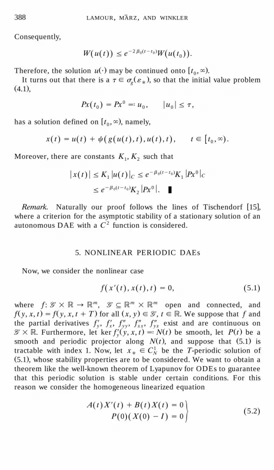
LAMOUR, MARZ, AND WINKLER¨388
Consequently,
W u t F ey2 b 0Ž tyt0 .W u t .Ž . Ž .Ž . Ž .0
Ž . w .Therefore, the solution u ? may be continued onto t , ` .0Ž .It turns out that there is a t g s «# , so that the initial value problemg
Ž .4.1 ,
0Px t s Px \ u , u F t ,Ž .0 0 0
w .has a solution defined on t , ` , namely,0
x t s u t q c g u t , t , u t , t , t g t , ` .Ž . Ž . Ž . Ž . .Ž .Ž . 0
Moreover, there are constants K , K such that1 2
yb Ž tyt . 00 0x t F K u t F e K PxŽ . Ž . CC1 1
yb Ž tyt . 00 0F e K Px .2
w xRemark. Naturally our proof follows the lines of Tischendorf 15 ,where a criterion for the asymptotic stability of a stationary solution of anautonomous DAE with a C 2 function is considered.
5. NONLINEAR PERIODIC DAEs
Now, we consider the nonlinear case
f x9 t , x t , t s 0, 5.1Ž . Ž . Ž .Ž .
where f : GG = R ª R m, GG : R m = R m open and connected, andŽ . Ž . Ž .f y, x, t s f y, x, t q T for all x, y g GG, t g R. We suppose that f and
the partial derivatives f X , f X , f Y , f Y , f Y exist and are continuous ony x y y x x y xXŽ . Ž . Ž .GG = R. Furthermore, let ker f y, x, t \ N t be smooth, let P t be ay
Ž . Ž .smooth and periodic projector along N t , and suppose that 5.1 istractable with index 1. Now, let x# g C1 be the T-periodic solution ofNŽ .5.1 , whose stability properties are to be considered. We want to obtain atheorem like the well-known theorem of Lyapunov for ODEs to guaranteethat this periodic solution is stable under certain conditions. For thisreason we consider the homogeneous linearized equation
A t X 9 t q B t X t s 0Ž . Ž . Ž . Ž .5.2Ž .5P 0 X 0 y I s 0Ž . Ž .Ž .

FLOQUET THEORY 389
with
A t [ f X x#X t , x# t , t , B t [ f X x#X t , x# t , t 5.3Ž . Ž . Ž . Ž . Ž . Ž . Ž .Ž . Ž .y x
Ž .and the monodromy matrix X T .
Ž .THEOREM 5.1. Let the monodromy matrix X T ha¨e all of its eigen¨al-� < < 4ues in z g C: z - 1 ; then the periodic solution x# is asymptotically stable
in the sense of Lyapuno .
Ž .Proof. First, we use Theorem 3.2 iii to find appropriate F g1 Ž Ž m.. Ž Ž m..C R, L C and E g C R, L C that are both T-periodic and nonsin-N
gular and transform the linear DAE
A t x9 t q B t x t s 0 5.4Ž . Ž . Ž . Ž . Ž .
into Kronecker normal form with constant coefficients:
yWI 0x9 t q x t s 0.Ž . Ž .ž / ž /0 I
In the next step we apply the same matrix functions F and E to thenonlinear equation. Before doing so, we shift the variables and split thelinear terms. Let
f x#X t q y , x# t q x , t s A t y q B t x q h y , x , t , 5.5Ž . Ž . Ž . Ž . Ž . Ž .Ž .
Ž .which defines a function h for x, y in some neighborhood of 0 andt g R. h is as smooth as f and satisfies
h 0, 0, t s 0, hX 0, 0, t s 0, hX 0, 0, t s 0 for all tŽ . Ž . Ž .y x
and
2< < < <h y , x , t F C x q y . 5.6Ž . Ž .Ž .
Ž . Ž Ž . . 1Furthermore, h y, x, t s h P t y, x, t , and again, for x g C , we useNŽ Ž . Ž . . ŽŽ . Ž . Ž . Ž . Ž . .h x9 t , x t , t as an abbreviation for h Px 9 t y P9 t x t , x t , t . Now,
we look for solutions of
A t x9 t q B t x t q h x9 t , x t , t s 0. 5.7Ž . Ž . Ž . Ž . Ž . Ž . Ž .Ž .
Ž . Ž . Ž . Ž .Scaling by E t and transforming x t s F t x t , we obtain
yWI 0x9 t q x t q h x9 t , x t , t s 0, 5.8Ž . Ž . Ž . Ž . Ž .Ž .ž / ž /0 I

LAMOUR, MARZ, AND WINKLER¨390
where
h y , x , t s E t h P t F t y y P t F9 t x , F t x , t .Ž . Ž . Ž . Ž . Ž . Ž .Ž . Ž .
The relation
X Xh y , x , t s E t h P t F t y y P t F9 t x , F t x , t P t F tŽ . Ž . Ž . Ž . Ž . Ž . Ž . Ž .Ž . Ž .y y
X Ž . Ž . Ž .shows that N [ ker A ; h y, x, t is satisfied, since ker P t F t syŽ . Ž . Ž .ker A t F t s ker A s N. Hence, relation 4.2 is fulfilled.
Ž .Furthermore, 5.6 implies that
2< < < <h y , x , t F C Py q x .Ž . Ž .Ž . Ž . Ž . Ž .Hence, Lemma 4.1 applies to the DAE 5.8 and x t s F t x t solves
Ž .5.7 .
Finally, let us illustrate the results by means of two cases. The first is asimple and transparent academic example.
EXAMPLE 1. Consider the DAE
X ¦x q x y x y x x q x y 1 sin t s 0Ž .1 1 2 1 3 3X ¥x q x q x y x x q x y 1 cos t s 0Ž . , 5.9Ž .2 1 2 2 3 3
2 2 §x q x q x y 1 s 01 2 3
which has the 2p-periodic solution
Tx# t s sin t , cos t , 0 . 5.10Ž . Ž . Ž .
Ž . � 4 3Since N l S x s 0 for all x g R ,
N [ z g R3 : z s 0, z s 0 ,� 41 2
S x [ z g R3 ; 2 x z q 2 x z q z s 0 ,Ž . � 41 1 2 2 3
Ž .the DAE has globally index 1. The DAE linearized along x# ? has thecoefficients
1 0 0 1 y1 ysin tA# t s , B# t s ,Ž . Ž .0 1 0 1 1 ycos tž / ž /0 0 1 y2 sin t y2 cos t y1

FLOQUET THEORY 391
and the monodromy matrix
1 0 0 2 y1 0X 2p s exp y2p ,Ž . 0 1 0 1 2 0½ 5ž / ž /0 y2 0 0 0 0
y2 p Ž2 " i. y4p Ž .has the eigenvalues l s e s e . Hence, the solution 5.10 is1, 2Ž .asymptotically stable in the sense of Lyapunov Fig. 1 .
Ž .EXAMPLE 2. We consider a small nonlinear network see Fig. 2 , whichŽ w x.realizes Voltage doubling see 1 .
The equations are given by
G F y x q xŽ .Ž .L 1 3x s y x q1 1C C1 1
1x s y x q x q E tŽ .Ž .2 2 3C R2 Q
10 s y x q x q E t q F y x q x y F xŽ . Ž . Ž .Ž . Ž .2 3 1 3 3RQ
FIG. 1. Constraint manifold and solution for Example 1.

LAMOUR, MARZ, AND WINKLER¨392
FIGURE 2.
with
w xC s C s 2.75 nF , R s0.1 MV , R g 1, `1 2 Q L
1y5 630 uG s , F u s5)10 e y 1 mA,Ž . Ž .L RL
tE t s 3.95 sin 2p , Ts0.064.Ž . ž /T
Here the periodic solution x can be calculated only numerically. For theparameter R s 10, we illustrate the solution in Figure 3.L
Ž .Solving the system 5.2 , the Monodromy matrix is given by
q0.958846945 q0.0388510935 0X T s .Ž . q0.0373520951 q0.922919983 0ž /y0.0373520951 y0.922919983 0
Žw x.Using the two-point boundary-value code MSHDAE 7 and approximat-ing the Monodromy matrix by internal differentiation, we obtain
q0.958857 q0.0388564 0X T s .Ž . q0.0373418 q0.922919925 0app ž /y0.0373418 y0.922919925 0
Ž . Ž .The eigenvalues of X T are 0.983001, 0.898766, 0, and those of X Tappare 0.983005, 0.898772, 0. Hence the considered solution is asymptoticallystable in the sense of Lyapunov. Here, as in general, it is not possible topresent a picture of the constraint manifold as in Example 1, since thismanifold depends on t and is given only implicitly.

FLOQUET THEORY 393
FIG. 3. Components x , x , x of the solution for Example 2.1 2 3

LAMOUR, MARZ, AND WINKLER¨394
6. CONCLUSIONS
No doubt our first illustrative example is extremely simple. In the caseŽ .where we have applied problems as in the second example , the situation
is not so clear. The state manifold is not known and can move in time.Ž .Furthermore, the solution x# ? to be analyzed can only be obtained
numerically. Our calculus allows us to proceed for DAEs with index 1Ž w x.exactly as for regular ODEs e.g., 14 . The resulting numerical methods
will inherit all difficulties typical of regular ODEs.Now the question arises whether our calculus can also be applied to
DAEs with a higher index. As the problem of linearization, which is thebasis for the Floquet theory, has been sufficiently solved for DAEs with
Žw x w x.index 2 in the meantime 10 , 16 , we are optimistic about this case,which, however, is considerably more complicated in its details.
REFERENCES
1. B. Barz and E. Suschke, ‘‘Numerische Behandlung eines Algebro-Differentialgleichungs-systems,’’ RZ-Mitteilungen 7, Humboldt-Universitat, Berlin, 1994.¨
2. M. Hanke, E. Griepentrog, and R. Marz, ‘‘Berlin Seminar on Differential-Algebraic¨Equations,’’ Seminarbericht 92-1, Humbolt-Universitat, Berlin, 1992.¨
3. M. Farkas, ‘‘Periodic Motions,’’ Springer, New York, 1994.4. G. Floquet, Sur les equations differentielles lineaires a coefficeints periodiques, Ann. Sci.´ ´ `
´ Ž .Ecole Norm. Sup. 12 1883 , 47]89.5. E. Griepentrog and R. Marz, ‘‘Differential-Algebraic Equations and Their Numerical¨
Treatment,’’ Teubner-Texte Math. 88, Teubner, Leipzig, 1986.6. J. Hale, ‘‘Ordinary Differential Equations,’’ Wiley, New York, 1969.7. R. Lamour, MSHDAE, www.mathematik.hu-berlin.derservrsoft.html, 1991.8. A. M. Lyapunov, ‘‘The General Problem of the Stability of Motion,’’ Taylor & Francis,
Ž .London, 1992. Originally: Kharkov, 1892, Russian .Ž .9. R. Marz, Numerical methods for differential-algebraic equations, Acta Numerica 1992 ,¨
141]198.10. R. Marz, On linear differential-algebraic equations and linearizations. APNUM 18¨
Ž .1995 , 267]292.11. P. C. Muller, Stabilitat mechanischer Systeme mit holonomen Bindungen, Z. Angew.¨ ¨
Ž .Math. Mech. 75 1995 , 593]594.12. L. S. Pontryagin, ‘‘Gewohnliche Differentialgleichungen,’’ Dt. Verl. Wiss., Berlin, 1965.¨13. R. M. M. Mattheij, R. Lamour, and R. Marz, On the stability behaviour of systems¨
Ž .obtained by index-reduction, J. Comp. Appl. Math. 56 1994 , 305]319.14. R. Seydel, ‘‘Practical Bifurcation and Stability Analysis: From Equilibrium to Chaos,’’
Springer, New York, 1994.15. C. Tischendorf, On the stability of solutions of autonomous index-1 tractable and
Ž .quasilinear index-2 tractable daes. Circuits Systems Signal Process 13 1994 , 139]154.16. C. Tischendorf, ‘‘Solution of Index-2 Differential Algebraic Equations and Its Application
in Circuit Simulation,’’ Ph.D. thesis, Humboldt University, Berlin, 1996.