Iterative solution of linear systems in electromagnetics (and not only): Experiences with CUDA

UnConventional High Performance Computing UnConventional High Performance Computing (UCHPC) 2010 workshop at:(UCHPC) 2010 workshop at:

Iterative Solution of Linear Systems inIterative Solution of Linear Systems inElectromagnetics (and not only):Electromagnetics (and not only):

Experiences with CUDAExperiences with CUDAD. De DonnoD. De Donno, A. Esposito, G. Monti, L. Tarricone, A. Esposito, G. Monti, L. Tarricone

Innovation Engineering DepartmentInnovation Engineering DepartmentUniversity of Salento University of Salento -- Lecce Lecce -- Italy Italy

August 30st, 2010August 30st, 2010

Danilo De DonnoDanilo De Donno –– University of Salento, Lecce, Italy University of Salento, Lecce, Italy

OutlineOutline

Background on CEM issues

Motivations and objectives

Design and implementation

Experimental results

Conclusions and ongoing work


BackgroundBackground

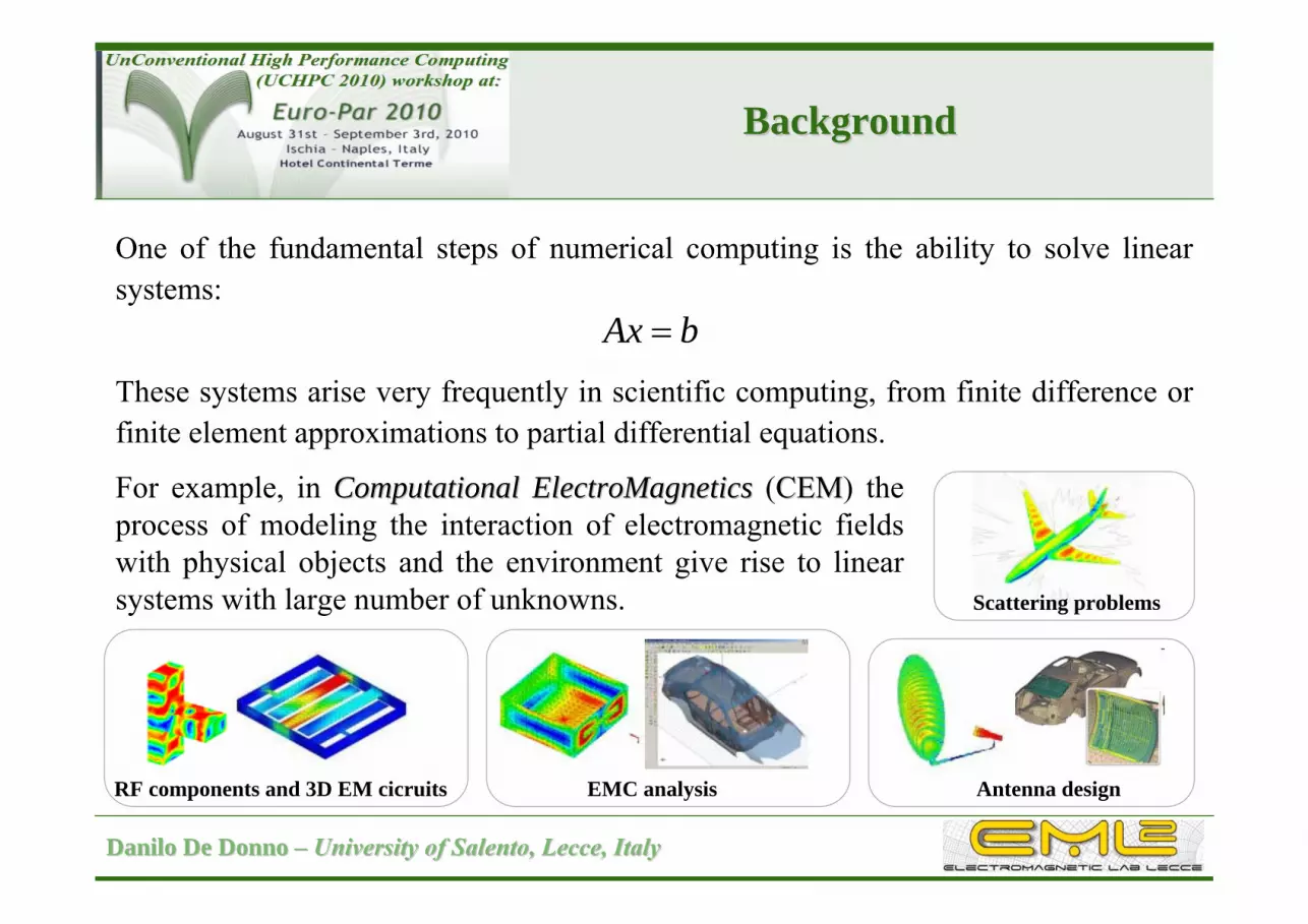
One of the fundamental steps of numerical computing is the ability to solve linear systems:

These systems arise very frequently in scientific computing, from finite difference or finite element approximations to partial differential equations.

Ax b

For example, in Computational ElectroMagneticsComputational ElectroMagnetics (CEMCEM) the process of modeling the interaction of electromagnetic fields with physical objects and the environment give rise to linear systems with large number of unknowns.

RF components and 3D EM cicruits EMC analysis Antenna design

Scattering problems


In CEM a key role is played by the Method of MomentsMethod of Moments (MoMMoM) which transforms the integral-differential Maxwell's equations into a linear system of algebraic equations.

Object discretizationObject discretization

MoMMoM--basedbasedEM simulatorEM simulator

Solve linear systemSolve linear system

Z I V

Z is the MoM impedance matrix containing the complexcomplex reaction terms between basis functions. In largelarge EM problems Z can be reduced to an unstructuredunstructured and significantly sparsesparsematrix without affecting the numerical accuracy.

ITERATIVE SOLVERSITERATIVE SOLVERS (i.e. CG, BiCG) are preferred in these cases.

Method of Moments (MoM)Method of Moments (MoM)linear systemslinear systems


ObjectiveObjective

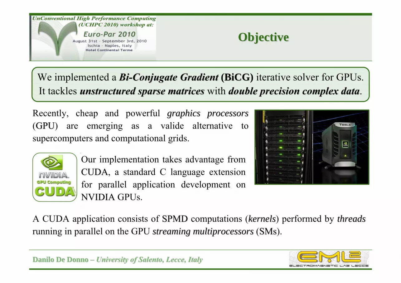
We implemented a BiBi--Conjugate GradientConjugate Gradient (BiCGBiCG) iterative solver for GPUs.It tackles unstructured sparseunstructured sparse matricesmatrices with double precision complexdouble precision complex datadata.

Our implementation takes advantage from CUDACUDA, a standard C language extension for parallel application development on NVIDIANVIDIA GPUs.

Recently, cheap and powerful graphics processorsgraphics processors(GPUGPU) are emerging as a valide alternative to supercomputers and computational grids.

A CUDA application consists of SPMDSPMD computations (kernelskernels) performed by threadsthreadsrunning in parallel on the GPU streaming multiprocessorsstreaming multiprocessors (SMsSMs).


The BiCG algorithm (1/2)The BiCG algorithm (1/2)

BiCGBiCG is a generalization of CGCG (Conjugate GradientConjugate Gradient) method.

CG methodCG method real symmetric matrices complex Hermitian matrices

BiCG methodBiCG method real non-symmetric matrices complex non-Hermitian matrices

Residual and biResidual and bi--residualresidual

Direction and biDirection and bi--directiondirection

PrePre--conditioned residual and biconditioned residual and bi--residualresidual

Initial residual errorInitial residual error

In the initialization phase of BiCG, the following variables are defined:

0 0 0 0

0 0 0 0

1 100 0 0

00

* *

**T

r b Ax r rp r p pd M r d M r

d r


The BiCG algorithm (2a/2)The BiCG algorithm (2a/2)

In the BiCG main loop, the following steps are repeated for each iteration:

1

1

1

1

1 1

*

i i

Hi i

ii

i i

i i i i

q A pq A p

p qx x p

STEP 1STEP 1

1. 1. Calculate the step lenght parameter and form the new solution esCalculate the step lenght parameter and form the new solution estimate.timate.


1

1

1

1

*

i i i i

i i i i

i i

i i

r r q

r r q

d M r

d M r

STEP 2STEP 2

2. 2. Update residual and biUpdate residual and bi--residual, with and without preconditioning.residual, with and without preconditioning.


The BiCG algorithm (2b/2)The BiCG algorithm (2b/2)


1

*Ti i i

ii

i

d r

STEP 3STEP 3

3. 3. Calculate the residual error Calculate the residual error ρρ and the biand the bi--conjugacy coefficient conjugacy coefficient ββ..


The BiCG algorithm (2c/2)The BiCG algorithm (2c/2)


1

1*

i i i i

i i i i

p d p

p d p

STEP 4STEP 4

4. 4. Update next direction and biUpdate next direction and bi--direction vectors.direction vectors.

Iteration is continued till the convergence criterion is satisfied:2

2

irb

Values of ε commonly used are 10-6 / 10-7.


The BiCG algorithm (2d/2)The BiCG algorithm (2d/2)


Design of the GPUDesign of the GPU--enabled BiCGenabled BiCG

In the GPU-enabled BiCG algorithm, the main loop execution is controlled on the host side, whereas the computations inside are performed on the GPU.

INITIALIZATIONINITIALIZATION consists in: reading and storing the system matrix

in a given sparse format; allocating data structures on the GPU

and calculating BiCG initial variables.

BiCG MAIN LOOP BiCG MAIN LOOP consists of the iterative invocation of parallel CUDA kernels performing the BiCG operations.

FINALIZATION FINALIZATION consists in retrieving final results from GPU global memory.


Implementation (1/3)Implementation (1/3)

Four basic CUDA kernels are enough to completely describe the BiCG main loop:

8·Nax+y (a scalar, x and y vectors)axpy

6·NElement-wise product of two vectorsE-w product

8·NScalar product of two vectors Dot product

8·nnzSparse matrix-vector productSpMV

FLOPSFLOPSDescriptionDescriptionOperationOperation

Recall that we are considering nonnon--symmetricsymmetric and nonnon--HermitianHermitian sparsesparse matrices with N rows and nnz non-zero complexcomplex coefficients.


Implementation (2a/3)Implementation (2a/3)

Supported sparse matrix formatsSupported sparse matrix formats CRSCRS (Compressed Row Compressed Row

StorageStorage) HYBHYB (hybrid ELLpackhybrid ELLpack--

COOrdinate formatCOOrdinate format)

Main modifications to the original codeMain modifications to the original code double precision complex matrix supportdouble precision complex matrix support CUDA grid, register number, shared and CUDA grid, register number, shared and

texture memory exploitation optimized for texture memory exploitation optimized for double precision complex data.double precision complex data.

SpMVSpMV – this CUDA kernel implements the Bell and Garland algorithm (*) which is the best performing code currently avaible for solving sparse matrix-vector product.

1

1

i i

Hi i

q A pq A p

(*) N. Bell and M. Garland: “Implementing sparse matrixImplementing sparse matrix--vector multiplication on throughput oriented vector multiplication on throughput oriented processorsprocessors”, In Supercomputing ’09, Nov. 2009.

Dot productDot product – cuBLAScuBLAS dot function doesn’t support double precision complex data, therefore we implemented it from scratch.To maximize performance we also adapted Mark Harris’ parallel parallel reductionreduction code (**) as the core of our code.

1

1 **

ii

i i

Ti i i

p qd r

(**) M. Harris, S. Sengupta, J.D. Owens: “Parallel prex sum (scan) with CUDAParallel prex sum (scan) with CUDA”, in GPU Gems 3, Nguyen H., Ed. Addison Wesley, August 2007.


Implementation (2b/3)Implementation (2b/3)


Implementation (3/3)Implementation (3/3)

E.w. product and axpyE.w. product and axpy – also in this case, the cuBLAS function provided by CUDA doesn’t support double precision complex data, therefore we implemented it from scratch.

1

1

i i

i i

d M r

d M r

1 1

1

1

1

1

*

*

i i i i

i i i i

i i i i

i i i i

i i i i

x x pr r qr r qp d pp d p

We defined a CUDA grid of 192 blocks192 blocks, each with 128 threads128 threads, to fully exploit GPU’s resources.

Threads load data from GPU global memory and perform calculations in parallel.

We optimized global memory access pattern to obtain completely coalesced loads and stores, thus minimizing latency.


Optimization strategiesOptimization strategies

In design and implementation of CUDA kernels we adopted the following optimization strategies:

CUDA on-chip shared memory exploitationshared memory exploitation for fast memory accesses;

register usageregister usage optimization;

loop unrollingloop unrolling;

texture memory exploitationtexture memory exploitation for caching data that are spatially closed together;

builtbuilt--in arraysin arrays to store complex data thus maximizing aligned memory spaces;

optimization of thread block dimensionthread block dimension to maximize multiprocessor occupancy.


Experiments and resultsExperiments and results

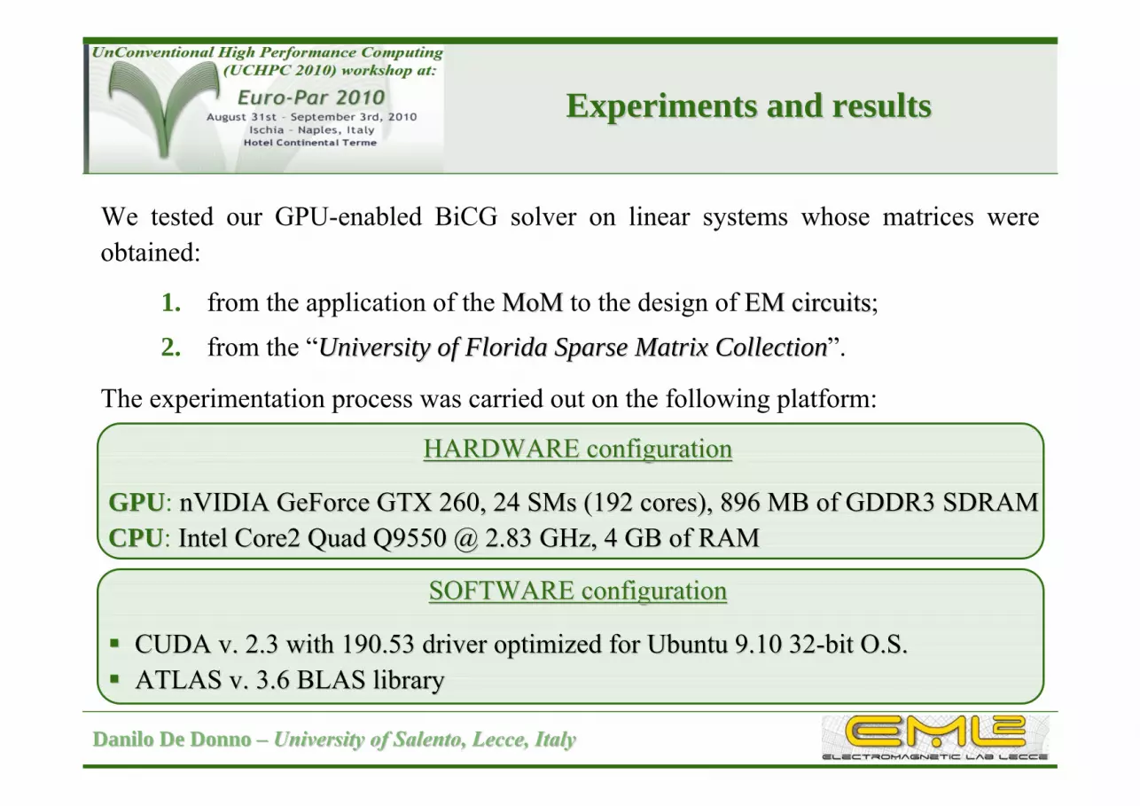
We tested our GPU-enabled BiCG solver on linear systems whose matrices were obtained:

1. from the application of the MoMMoM to the design of EM circuitsEM circuits;

2. from the “University of Florida Sparse Matrix CollectionUniversity of Florida Sparse Matrix Collection”.

The experimentation process was carried out on the following platform:

HARDWARE configurationHARDWARE configuration

GPUGPU: nVIDIA GeForce GTX 260, 24 SMs (192 cores), 896 MB of GDDR3 SDRAnVIDIA GeForce GTX 260, 24 SMs (192 cores), 896 MB of GDDR3 SDRAMMCPUCPU: Intel Core2 Quad Q9550 @ 2.83 GHz, 4 GB of RAMIntel Core2 Quad Q9550 @ 2.83 GHz, 4 GB of RAM

SOFTWARE configurationSOFTWARE configuration

CUDA v. 2.3 with 190.53 driver optimized for Ubuntu 9.10 32CUDA v. 2.3 with 190.53 driver optimized for Ubuntu 9.10 32--bit O.S.bit O.S. ATLAS v. 3.6 BLAS libraryATLAS v. 3.6 BLAS library


EMEM--MoM matrices: case studyMoM matrices: case study

As to EM matrices derived from MoM, they concern the design of branch-line couplers in microstrip technology, which are four ports devices widely adopted in microwave and millimetre-wave applications like power dividers and combiners.

More specifically, the analyzed layout consists of two branch-line couplers connected by means of a 360° microstrip line and operating in the 2.5-3.5 GHz frequency band.


EMEM--MoM matrices: results (1/3)MoM matrices: results (1/3)

The figure below shows the convergence times of the sequential (on CPU) and parallel (on GPU) BiCG algorithm when varying the number of system unknowns, for two different sparse matrix storage formats (HYB and CRS).

The desired matrix sparsity pattern was obtained by mean of a thresholding operation. We kept the percentage of non-zero elements to about 5% of the total number of entries while maintaining a good accuracy of the final solution.

The adopted BiCG stopping criterion:

72

2

10ir

b


EMEM--MoM matrices: results (2/3) MoM matrices: results (2/3)

In the figure below we show BiCG performance in terms of number of floating point operations (FLOPs) per second.

20.7424.768E+323.6923.6928.5728.5710E+3

21.3623.796E+311.512.8 4E+3

1.843.012E+3

SpeedSpeed--Up Up HYBHYB

SpeedSpeed--Up Up CRSCRS

Problem Problem Size (N)Size (N)

Achieved speed-ups are higher when matrix dimension allows for an optimum exploitation of hardware resources. CRS has the maximum benefits from GPU parallelization, achieving a speed-up of almost 3030.


EMEM--MoM matrices: results (3/3) MoM matrices: results (3/3)

In all EM matrices we analyzed, CRSCRS format always produces faster results because of the high variability of the non-zero number per row.

As figure shows, the number of non-zeros per row varies widely in typical EM-MoM matrices, so CRSCRS performs better than HYBHYB. Indeed, HYB storage format is suitable when the non-zero distribution is quite compact.


FLORIDA matrices (1/2)FLORIDA matrices (1/2)

We identified ten complex sparse matrices, belonging to different research areas and exhibiting different size, sparsity pattern and number of non-zeros.

In order to demonstrate the validity of our GPU-enabled BiCG implementation, we conducted some tests on sparse matrices taken from “The University of Florida Sparse The University of Florida Sparse Matrix CollectionMatrix Collection“.


FLORIDA matrices (2/2)FLORIDA matrices (2/2)

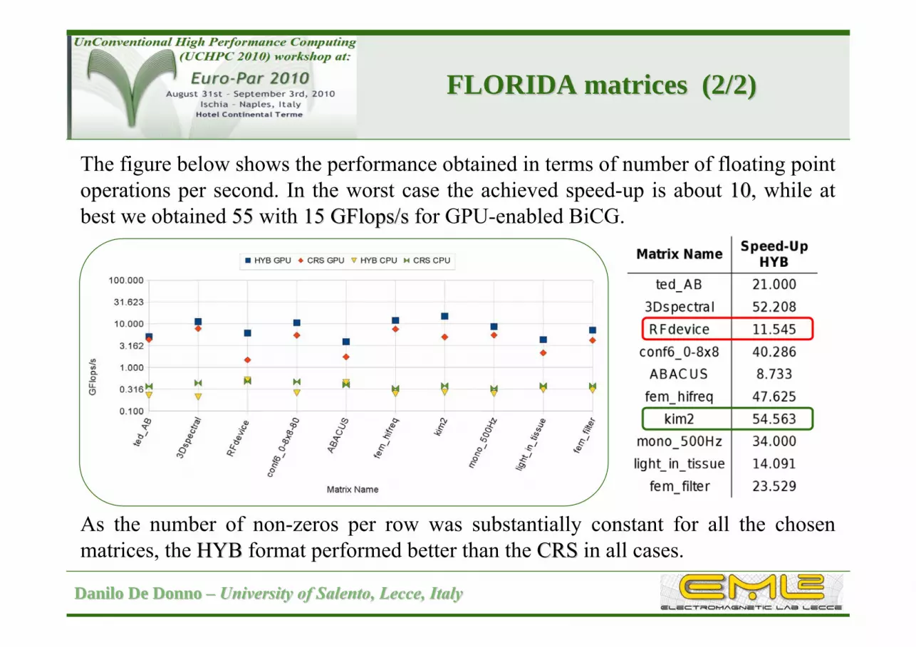
The figure below shows the performance obtained in terms of number of floating point operations per second. In the worst case the achieved speed-up is about 1010, while at best we obtained 5555 with 15 GFlops/s15 GFlops/s for GPU-enabled BiCG.

As the number of non-zeros per row was substantially constant for all the chosen matrices, the HYBHYB format performed better than the CRS CRS in all cases.


Conclusions and ongoing workConclusions and ongoing work

In this work, the achievement of peak-performance for EM solvers through the use of the inexpensive and powerful GPUs has been investigated.

Taking advantage from CUDA library, we implemented a BiCG algorithm which tackles unstructured sparse matrices with double precision complex data and manages two sparse matrix formats.

It has been tested on several research area problems. Results in terms of convergence behaviour and GPU vs. CPU performance have been provided as a validation and assessment of solver efficiency.

As further improvements to our work we plan to:1. develop and test other sparse matrix formats suitable for EM-MoM problems;2. integrate complex and well known pre-conditioners in our BiCG algorithm;3. compare our code with efficient BiCG solvers adopting Intel MKL BLAS library

on multi-core architectures;4. hybridize our BiCG code to support together multi-GPU and multi-core CPUs.

ContactsContacts

Danilo De DonnoDanilo De [email protected]@unisalento.it

Alessandra EspositoAlessandra [email protected]@unisalento.itit

Giuseppina MontiGiuseppina [email protected]@unisalento.itit

Luciano TarriconeLuciano [email protected]@unisalento.it

wwwwww.electromagnetics..electromagnetics.uunile.itnile.it

Iterative solution of linear systems in electromagnetics (and not only): Experiences with CUDA

Documents

Transcript of Iterative solution of linear systems in electromagnetics (and not only): Experiences with CUDA