HAL Id: hal-01136770https://hal.archives-ouvertes.fr/hal-01136770

Submitted on 1 Apr 2015

HAL is a multi-disciplinary open accessarchive for the deposit and dissemination of sci-entific research documents, whether they are pub-lished or not. The documents may come fromteaching and research institutions in France orabroad, or from public or private research centers.

L’archive ouverte pluridisciplinaire HAL, estdestinée au dépôt et à la diffusion de documentsscientifiques de niveau recherche, publiés ou non,émanant des établissements d’enseignement et derecherche français ou étrangers, des laboratoirespublics ou privés.

Performance evaluation of CUDA programming for5-axis machining multi-scale simulation

Felix Abecassis, Sylvain Lavernhe, Christophe Tournier, Pierre-Alain Boucard

To cite this version:Felix Abecassis, Sylvain Lavernhe, Christophe Tournier, Pierre-Alain Boucard. Performance evalu-ation of CUDA programming for 5-axis machining multi-scale simulation. Computers in Industry,Elsevier, 2015, 71, pp.1-9. �10.1016/j.compind.2015.02.007�. �hal-01136770�

Performance Evaluation of CUDA programming for5-Axis machining multi-scale simulation

Felix Abecassisa, Sylvain Lavernhea, Christophe Tourniera,∗, Pierre-AlainBoucardb

aLURPA, ENS Cachan, Univ Paris-Sud61 Avenue du president Wilson, F-94235 Cachan, France

bLMT Cachan, ENS Cachan/CNRS/PRES UniverSud Paris61 Avenue du president Wilson, F-94235 Cachan, France

Abstract

5-Axis milling simulations in CAM software are mainly used to detect collisions

between the tool and the part. They are very limited in terms of surface to-

pography investigations to validate machining strategies as well as machining

parameters such as chordal deviation, scallop height and tool feed. Z-buffer or

N-Buffer machining simulations provide more precise simulations but require

long computation time, especially when using realistic cutting tools models in-

cluding cutting edges geometry. Thus, the aim of this paper is to evaluate

Nvidia CUDA architecture to speed-up Z-buffer or N-buffer machining simula-

tions. Several strategies for parallel computing are investigated and compared

to single-threaded and multi-threaded CPU, relatively to the complexity of the

simulation. Simulations are conducted with two different configurations includ-

ing Nvidia Quadro 4000 and Geforce GTX 560 graphic cards.

Keywords: 5-Axis milling, Machining simulation, GPU computing, GPGPU,

CUDA architecture

1. Introduction

All manufactured goods present surfaces that interact with external ele-

ments. These surfaces are designed to provide sealing or friction functions, op-

∗Corresponding author Tel.: +33 1 47 40 27 52; Fax: +33 1 47 40 22 20Email address: christophe.tournier@ens-cachan.fr (Christophe Tournier)

Preprint submitted to Elsevier April 1, 2015

tical or aerodynamics properties. The technical function of the surface requires

specific geometrical deviations which can be performed with specific manufac-

turing process. In particular, to reduce the cycle time of product development,

it is essential to simulate the evolution of geometrical deviations of surfaces

throughout the manufacturing process. Currently, simulations of the machined

surfaces in CAM software are very limited. These simulations are purely ge-

ometric where cutting tools are modeled as spheres or cylinders without any

representation of cutting edges.

In addition, these simulations do not include any characteristic of the actual

process that may damage the surface quality during machining such as feedrate

fluctuations, vibrations and marks caused by cutting forces and tool flexion,

geometrical deviations induced by thermal expansion, etc. Many models exist

in the literature [1][2][3], but given their complexity and specificity, they often

require very high computation capability and remains academic models. Fi-

nally, CAM software simulations do not provide the required accuracy within

a reasonable computation time and the selection of an area in which the user

wishes to have more precision is impossible.

However, there are many methods to perform machining simulations in the

literature: methods based on a partition of the space by lines [4], by voxels [5]

or by planes [6], methods based on meshes [7], etc. If we consider the Z-buffer

or N-buffer methods applied to a realistic description of both the tools and

the machining path, earlier work have shown that it is possible to simulate the

resulting geometry on small portions of the surface in a few minutes [8][9]. Sim-

ulation results are very close to experimental results but the simulated surfaces

have an area of a few square millimeters with micrometer resolution (Fig. 1).

Therefore, the limits in terms of computing capacity and simulation methods

restrict the realistic simulations of geometrical deviations.

A faster simulation could help to take into account more complex and realis-

tic geometrical model for the tool and its displacements and rotations onto the

workpiece and introduce non purely geometrical model but mechanical behav-

ior with cutting loads, tool and workpiece flexions. Polishing process could be

2

investigated considering abrasive particles as elementary cutting tools, increas-

ing drastically the number of intersection tests without increasing the time for

simulation.

µm

0

1

2

3

4

5

6

7

Figure 1: Simulation versus experimental results for 5-Axis milling with ball-end tool

Regarding the hardware, NVIDIA has recently developed CUDA, a par-

allel processing architecture for faster computing performance, harnessing the

power of GPUs (graphics processing units) by using GPGPU. GPGPU (general-

purpose computing on graphics processing units) is the utilization of a GPU,

which typically handles computation only for computer graphics, to perform

computation in applications traditionally handled by the central processing unit

(CPU). GPU’s technology in the CAD/CAM community is widely used but the

CUDA technology is just beginning in the field of machining.

Few works can be underlined such as those proposed in [10] dealing with

the acceleration of a specific tool path algorithm called virtual digitizing. It is

based on a Z-map approach and similar to the inverse Z-buffer developed in [11]

[12] which is suited to parallel processing. They study in particular the influ-

ence of the calculations in single or double precision on performances on both

GeForce or Quadro devices. Kaneko et al. have also used the CUDA technology

to speed-up the cutter workpiece engagement in 5-Axis machining [13]. They

did not investigate the traditional approach based on Voxelmap or Z-buffer but

a novel approach based on swept volume, discretization of the tool flutes and a

polygonal approximation of the workpiece. Inui et al. compared two GPU based

acceleration methods for the geometric 3-Axis milling simulation: one based on

3

the depth buffer and the other based on the CUDA architecture [14]. Regardless

of the computation speed with CUDA, limits can be reached because of costly

data exchanges between CPU and GPU memories. Hence speed-up seems to be

efficient for small toolpath regardless of the tool size.

The aim of this paper is thus to propose a calculation scheme harnessing

the CUDA parallel architecture to reduce the computation time despite the

very large number of elementary computations. Within the multi-scale simula-

tion context, this consists in proposing the best distribution of the calculation

according to the configuration of the case studies and especially the zoom level.

After having presented constraints related to the use of the CUDA architec-

ture, the machining simulation algorithm to be parallelized is recalled. Then,

different solutions to the problem of parallelization with CUDA are investigated.

Finally a comparison of the computing time between GPU and CPU processors

is proposed on several 3- and 5-Axis milling examples.

2. Compute unified device architecture

CUDA is a parallel computing platform that unlocks programmability of

NVIDIA graphic cards in the goal of speeding up the execution of algorithms

exhibiting a high parallelization potential. Algorithms are written using a mod-

ified version of the ANSI C programming language (CUDA C) and can conse-

quently be executed seamlessly on any CUDA capable GPU [15].

The strength of the CUDA programming model lies in its capability of

achieving high performance through its massively parallel architecture (Fig.

??). In order to achieve high throughput, the algorithm must be divided into

a set of tasks with minimal dependencies. Tasks are mapped into lightweight

threads which are scheduled and executed concurrently on the GPU. Thirty-two

threads are grouped to form a warp. Threads within the same warp are always

executed simultaneously, maximum performance is therefore achieved if all the

32 threads are executing the same instruction at each cycle. Warps are them-

4

selves grouped into virtual entities called blocks, the set of all blocks forms the

grid, representing the parallelization of the algorithm. Threads from the same

block can be synchronized and are able to communicate efficiently using a fast

on-chip memory, called shared memory, whereas threads from different blocks

are executed independently and can only communicate through global (GDDR)

memory of the GPU.

The number of threads executing simultaneously can be two orders of mag-

nitude larger than on a classical CPU architecture. As a consequence, task

decomposition should be fine-grained opposed to the traditional coarse-grained

approach for CPU parallelization. The combination of this execution model and

memory hierarchy advocates a multi-level parallelization of the algorithm with

homogeneous fine-grained tasks, dependent tasks should be mapped to the same

warp or block in order to avoid costly accesses to global memory. In order to

harness the power of the massively parallel architecture of GPUs, a complete

overhaul of the algorithm is often required [16].

Figure 2: Cuda architecture

5

The scalability of the CUDA programming models stems from the fact that,

thanks to this fine-grain task model, the number of threads to execute gener-

ally exceeds the number of execution units on the GPU, called CUDA cores,

for those threads. As more CUDA cores are added, e.g. through hardware

upgrades, performance will increase without requiring changes to the code. An-

other benefit of this fine-grained decomposition is the ability to hide latency, if

a warp is waiting for a memory access to complete, the scheduler can switch to

another warp by selecting it from a pool of ready warps. This technique is called

thread level parallelism (TLP). Latency hiding can also be done within a thread

directly, by firing several memory transactions concurrently, this technique is

called instruction level parallelism (ILP).

Despite continuous efforts by NVIDIA to improve the accessibility of CUDA,

the learning curve remains steep. Attaining high performance requires careful

tuning of the algorithm through a detailed knowledge of the CUDA execution

model.

3. Computation algorithm

The computation algorithm relies on the Z-buffer method [4]. This method

consists in partitioning the space around the surface to be machined in a set

of lines which are equally distributed in the x-y plane and oriented along the

z-axis. The machining simulation is carried out by computing the intersections

between the lines and the tool along the tool path. The geometry of the tool is

modeled by a sphere or a triangular mesh including cutting edges which allows

to simulate the effect of the rotation of the tool on surface topography.

The tool path is whether a 3-axis tool path with a fixed tool axis orientation

or a 5-Axis tool path with variable tool axis orientations. In order to simulate

the material removal, intersections with a given line are compared and the lowest

is registered (Fig. 3).

The complete simulation requires the computation of the intersections be-

tween the N lines and the T triangles of the tool mesh at each tool posture P

6

on the tool path. The complexity C of the algorithm is thus defined by :

C = N × T × P (1)

0.1mm

0.02mm

0.05

mm

Figure 3: Z-buffer simulation method and cutting edge

If we consider a finish operation on a 5 mm x 5 mm patch of surface with a

resolution of 3 µm, this leads to 2,250,000 lines. The tool mesh contains 3000

triangles and the tool path contains 70,000 postures including the tool rotation

around the spindle axis with a discretization step of 0.2 degrees. The number of

intersections to compute is equal to 4.7 ·1014. This technique can be accelerated

by decreasing the number of tests by first calculating the intersection with the

bounding box of the tool and using data structures such as bounding volume

hierarchy [17] or binary space partitioning trees [18].

In the case of Z-buffer, all lines are oriented in the same direction which

allows many optimizations on both the number of intersection tests to be per-

formed and the number of operations required for each test. For each triangle,

its projection on the grid and its 2D bounding box is calculated (Fig. 4). The

7

lines outside the bounding box (shaded circles) are not tested, they can not have

an intersection with the triangle. A double loop is then performed to test the

intersection of each line within the bounding box with the 2D projection of the

triangle. The lines may intersect with the triangle (green) or not (red). If the

intersection exists, the height is calculated and then compared with the current

height of the line.

Figure 4: 2D bounding box

As there are no dependancies between the milling process at different loca-

tions on the tool path, each of these intersections could be carried out simulta-

neously. However, due to memory limitations and tasks scheduling, the parallel

computing of these intersections on graphics processing units with CUDA has

to be done carefully.

4. Line triangle intersection issues

The intersection algorithm is using the barycentric coordinates to check

whether the intersection point with the line is inside the triangle or not. This

requires to position the triangle relative to the line. For example, for a trans-

lation of the cutting tool, computing the reference frame (u and v coordinates)

formed by the two edges of the triangle can be done before or after the trans-

lation. Adding a large number (the coordinates of the translation) and a small

8

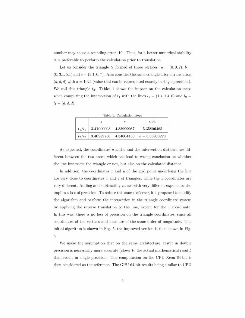
number may cause a rounding error [19]. Thus, for a better numerical stability

it is preferable to perform the calculation prior to translation.

Let us consider the triangle t1 formed of three vertices: a = (0, 0, 2), b =

(0, 3.1, 5.1) and c = (3.1, 0, 7). Also consider the same triangle after a translation

(d, d, d) with d = 1024 (value that can be represented exactly in single precision).

We call this triangle t2. Tables 1 shows the impact on the calculation steps

when computing the intersection of t1 with the lines l1 = (1.4, 1.4, 0) and l2 =

l1 + (d, d, d).

Table 1: Calculation steps

u v dist

t1/l1 3.41000008 4.33999967 5.35806465

t2/l2 3.40989756 4.34004163 d+ 5.35803223

As expected, the coordinates u and v and the intersection distance are dif-

ferent between the two cases, which can lead to wrong conclusion on whether

the line intersects the triangle or not, but also on the calculated distance.

In addition, the coordinates x and y of the grid point underlying the line

are very close to coordinates x and y of triangles, while the z coordinates are

very different. Adding and subtracting values with very different exponents also

implies a loss of precision. To reduce this source of error, it is proposed to modify

the algorithm and perform the intersection in the triangle coordinate system

by applying the reverse translation to the line, except for the z coordinate.

In this way, there is no loss of precision on the triangle coordinates, since all

coordinates of the vertices and lines are of the same order of magnitude. The

initial algorithm is shown in Fig. 5, the improved version is then shown in Fig.

6.

We make the assumption that on the same architecture, result in double

precision is necessarily more accurate (closer to the actual mathematical result)

than result in single precision. The computation on the CPU Xeon 64-bit is

then considered as the reference. The GPU 64-bit results being similar to CPU

9

(gx, gy, 0)(0, 0, 0)

Translation(tx, ty, tz)

distance d

Figure 5: Initial algorithm

(0, 0, 0)

Inverse Translation(-tx, -ty, 0)

d

Triangle

(gx, gy, 0)

Z translation(0, 0, tz)

Figure 6: Improved algorithm

10

in 64-bit, only the results on GPU 32-bit are presented. The case of study is

spiral and the result on the GPU is shown Fig. 7. The error shown is absolute,

for lines of initial height equal to 1000. Fig. 7 shows that in single precision,

the improved algorithm generates numerical errors 100x smaller than the initial

one. Consider for instance the machining simulation of a car bumper, given

Z-buffer lines of 1000 mm height, the error due to single precision is 0.001mm

with the initial algorithm and 0.00001mm with the improved one. Thus the

improved algorithm is used in further computations.

2

4

6

8

10

12 x104

-2 -1.5 21.510.50-0.5-1

x10-3

Fre

quen

cy

Absolute error

0.5

1.0

1.5

2.0

2.5

3.0 x104

-4 -3 43210-1-2x10-5

Fre

quen

cy

Absolute error

Figure 7: Single precision error for initial and improved algorithm

5. Parallel computation strategies

In the case of parallel execution, computation time is always limited by the

longest run. A long running thread can slowdown an entire warp, or worse, an

entire block. If the granularity of tasks is too high, this situation is more likely to

occur. The CUDA scheduler present on each graphics card is optimized for the

processing of a set of tasks having homogeneous complexities. In many cases,

this choice proves to be very effective. However in cases where the execution

time per task has a large variance, this method may not be optimal.

The basic algorithm consists in determining whether there is an intersection

between a line and a triangle associated to a position of the tool. Given these

11

three variables on which the algorithm iterates during the sequential compu-

tation, there are numerous possible combinations to affect threads and browse

the set of lines, triangles and positions. These combinations may generate un-

favorable cases in terms of parallelization and computational time. The most

interesting possibilities are summarized in Table 2 and developed hereafter.

Table 2: Different strategies

Line: One thread = One line

For each position For each triangle

For each triangle For each position

Intersection Intersection

Coarse: One thread = One position

For each triangle

For each line

Intersection

Inverted: One thread = One triangle

For each position

For each line

Intersection

Fine: One thread = One triangle for one pos.

For each line

Intersection

5.1. The line approach

Each CUDA thread is assigned to a line of the Z-buffer grid. A thread

calculates the intersection of the line with the tool triangles for all positions

along the path. To reduce the number of intersection tests, the intersection

with the global bounding box of the tool in a given position is first calculated.

12

If there is intersection, each triangle of the tool is then tested because a finer

bounding box cannot be used (Fig. 4). The advantage of this approach is that

there is no need to use atomic operations since the minimum height of cut for

each line is calculated by a single thread. However, for each position of the tool,

the transformation matrix must be computed which significantly increase the

number of calculations. Finally, this approach leads to longer computation time

and is not further considered.

Then, we only consider strategies that allow reducing the amount of required

calculations, i.e. those that reduce the calculation area by fine bounding box

and that let the geometric transformation (to position the mesh relatively to

the lines) outside the thread.

5.2. The tool position approach (coarse)

Each thread is assigned to a position of the tool and applies the Z-buffer

algorithm for each triangle of the tool mesh for this position. The granularity of

tasks is high: if the amount of triangles to be processed is large, each thread will

run for a long time. If the computation time between threads is heterogeneous,

some threads of a warp may no longer be active, and therefore the parallelism

is lost. A thread may affect the cutting height of several lines so a line can

be updated by multiple threads and global memory access conflicts appear.

Atomic operations proposed by CUDA are then used to allow concurrent update

of the height of the lines. This method is the one implemented in the CPU

configuration.

5.3. The tool triangle approach (inverted)

Each thread is assigned to a triangle of the tool mesh and applies the Z-buffer

algorithm for the triangle for all positions along the path. In the case of the

3-axis machining, the dimensions of the triangle projection on the grid remain

constant which allows optimization possibilities. However, in 5-Axis milling,

this property is no longer valid. Each position involves a new transformation

matrix to be recovered in memory which increases significantly the number of

13

memory transactions. This method is advantageous in the case of a 3-axis tool

path but is not suited for 5-Axis tool path. The same remarks apply the previous

approach on the granularity of tasks and conflicts in global memory access.

5.4. The triangle and position approach (fine)

In this approach, each thread is assigned to a single triangle in one position.

As the granularity is smaller, the risk of a bad balance workload disappears.

However, in return the number of threads is much higher: the management

and scheduling of billions of threads involve additional workload for the task

scheduler CUDA and thus a significant increase in computation time.

6. Numerical investigations

6.1. Case study

Different configurations of trajectories and tools have been used for test-

ing. A first setting, called random (Fig. 8(a)), for which random positions are

generated on a plane and a second setting, where a plane is machined along a

downward spiral called spiral (Fig. 8(b)). In both cases, the ball-end tool is 100

times smaller compared to the dimensions of the surface.

A roughing operation with a torus tool (Fig. 8(c)) and a 5-Axis finishing

operation with a ball end tool (Fig. 8(d)) of a pseudo blade part are also

proposed in the benchmark. At last, a small scale simulation benchmark, called

Cutting edge, is proposed with the mesh of a ball end mill including worn cutting

edges and spindle rotation (Fig. 8(e)) which lead to numerous tool positions

and large tool mesh size (Table 3).

One of the objectives is to be able to dynamically zoom on the part and

update the simulation. Thus the grid size is constant and set to 1024x1024

lines, regardless of the zoom factor. Therefore, the above configurations are

also studied with or without a zoom on the surface, which changes the size of

the problem (Tables 3 and 4).

14

Table 3: Macro geometry (without zoom)

Case Tool position P Tool Mesh size T

Random 200000 sphere 320

Spiral 200000 sphere 1984

Roughing 47837 torus 25904

Finishing 53667 sphere 12482

Cutting edge 144001 local edges 36389

Table 4: Micro geometry (with zoom)

Case Tool position P Tool Mesh size T

Random 135 sphere 320

Spiral 206 sphere 1984

Roughing 619 torus 25904

Two different dardware configurations are considered:

• CAD/CAM configuration:

– CPU1: Intel Xeon X5650 2.67 GHz, 6 cores, 12 virtual cores, SSE,

64 Gflops DP, ($1000)

– GPU1: Nividia Quadro 4000 0.95 GHz, 8 multiprocessors, 256 CUDA

Cores, 243 Gflops DP, 486 SP, ($700)

• GAMING configuration:

– CPU2: AMD Phenom II X4 955 (3.2 GHz), 4 cores, SSE, 32 Gflops

DP, ($150)

– GPU2: Nividia GeForce GTX 560 1.76 GHz, 8 multiprocessors, 384

CUDA Cores, 1264 Gflops SP, ($220)

Thus, from a purely theoretical standpoint, the GPU Quadro 4000 is approxi-

mately 4x faster than the Xeon CPU in 64-bit and the GPU GTX 560 40x faster

than the AMD Phenom. This will help us to discuss the results in section 6.3.

15

(a) random (b) spiral

(d) finishing (c) roughing

(e) cutting edge

Figure 8: Cases of study

16

6.2. Discussion on computation strategies

Excluding cases of zoom, GPU implementation is on average 5 times faster

than the CPU implementation with the engine GPU Coarse (1 thread handles

all triangles in one position).

When the number of triangles in the mesh of the tool is too low, the number

of threads used in the engine GPU Inverted is much lower than the number

of threads that can be executed simultaneously on all multiprocessors. Perfor-

mance is worse (random). When the number of triangles increases (random to

spiral, spiral to roughing and roughing to cutting edge), performance improves

accordingly. Furthermore, as mentioned earlier, acceleration with bounding box

can’t be done in 5-Axis machining (finishing) which leads to smaller speed-up

compared to 3-axis operations.

With the engine GPU Fine (1 thread processes one triangle in one position),

there are too few lines in the bounding box of each triangle because the triangles

are very small compared to the size of the grid. Each thread is little busy and

time is lost to launch these threads.

Table 5: Macro geometry N=1024*1024 ; 64 bits ; CAD/CAM configuration

Case Time (ms) GPU Speed-up

CPU Coarse Inverted Fine

Random 366 5.3 0.4 3

Spiral 1061 4.3 2.9 2.1

roughing 7891 5.1 5.1 1.7

Finishing 11542 4.9 3.6 4.2

Cutting edge 22882 8.3 7.8 2.3

In micro geometry configurations, the GPU speed-up does not meet expec-

tations (Table 4). Since the number of positions with zoom is much lower than

the number of threads that can be executed simultaneously on all GPU multi-

processors, the granularity of the simulation engine GPU Coarse is too high:

the available parallelism is not exploited. The computation engine must exhibit

a much finer granularity, such as the GPU Fine engine, that should be used

17

to make best use of the number of threads.

Table 6: Micro geometry N=1024*1024 ; 64 bits ; CAD/CAM configuration

Case Time (ms) GPU Speed-up

CPU Coarse Inverted Fine

Random 168 0.14 0.22 3.1

Spiral 321 2.0 1.6 4.7

roughing 943 0.3 3.9 3.2

Performance tests with or without zoom show that the CUDA kernel must

be chosen depending on the simulation configuration. Conversely, it is not a

problem with the CPU engine because the number of available threads is much

lower than the number of positions. During the initial implementations, the

acceleration factor was more important between GPU and CPU, but successive

optimizations have, systematically, further improved the CPU engine rather

than GPU implementations. The difference between the two versions is reduced

over the optimizations. We thought that a fair and accurate comparison be-

tween CPU and GPU needs to have two optimized versions of the code for both

architectures.

6.3. 32/64-Bit implementation

Both configurations have been tested on the same case study in order to

compare 32-bit and 64-bit performances. Achieving high performance on CUDA

requires limiting access to the global memory, or in double precision, these

accesses are doubled. In addition, the number of registers used in a kernel has a

very important impact on the number of threads that can be launched by block,

and therefore on performances. Moreover, only some CUDA cores can run 64-bit

floating-point operations. The 64-bit implementation uses 59 registers against

33 for the 32-bit implementation, thus the potential parallelism is lower because

the size of the register bank on each multiprocessor is limited.

As expected, the results (Tables 7 and 8) show that both GeForce and

Quadro cards are less powerful in 64-bit computing. The loss of performance of

18

the GeForce card in 64-bit computing is greater than the Quadro. Indeed, the

Quadro is optimized for scientific calculations while the GeForce is a consumer

card for video games. In terms of speed-up, results are of the same order with

the theoretical speed-up established in section 6.1.

Table 7: 32/64-Bit speed-up with Coarse approach CAD/CAM configuration

Case Time (ms) Quadro 4000

CPU 64-bit 32-bit 64-bit

Random 366 8.5 5.3

Spiral 1061 6.4 4.3

roughing 7891 8.4 5.1

Finishing 11542 7.6 4.9

Table 8: 32/64-Bit speed-up with Coarse approach GAMING configuration

Case Time (ms) GeForce 560 Ti

CPU 64-Bit 32-bit 64-bit

Random 1260 28.3 12.8

Spiral 4634 47.8 9.1

roughing 25160 39.8 8.7

Finishing 30603 27.2 7.7

19

In order to compare the devices with their best performances, speed-up rela-

tives to the Xeon CPU computation time are proposed in Table 9. Calculations

performed by the 32-bit GeForce card are about twice faster than 64-bit cal-

culations of the Quadro. Theoretically, the speed-up with the 32-bit GeForce

should be better and it could have been the case in a third configuration includ-

ing both the Xeon CPU and the GeForce card. As discussed before, this raises

the problem of computation accuracy but the improved algorithm (section 4)

can ensure relatively low numerical disparities. One can imagine using 32-bit

mode to explore different areas of the part. As the user is gradually zooming,

the vertical amplitude of the simulation decreases, so the z-buffer lines height

decreases as well as simulation error (section 4). Finally, a 64-bit computing

simulation is launched once a specific area is chosen.

Table 9: 32/64-bit speed-up with Coarse approach

Case Time (ms) GeForce 560 Ti Quadro 4000

CPU Xeon 32-bit 64-bit

Random 366 7.6 5.3

Spiral 1061 10.1 4.3

roughing 7891 11.1 5.1

Finishing 11542 8.3 4.9

6.4. CAM software comparison

On the other hand, an industrial configuration is proposed, which consists in

the 3-axis machining of a plastic injection mold to produce polycarbonate optical

lenses for ski mask. The finishing simulation is compared to an industrial CAM

software simulation in terms of visible defects and computation time. The tool

path contains 7.10e5 tool positions and the tool is considered as a canonical

sphere.

Because of the numerical connection of CAD patches, a tangency disconti-

nuity has been introduced in the toolpath along the vertical symmetry axis in

the middle of the lens. The machining simulation should emphasize the result-

ing geometrical deviation. Despite using the best settings offered by the CAM

20

software, the rendering of the simulation is not enough precise to detect the

groove generated during tool path computation (Fig. 9). The processing time

for this simulation is 450s. On the other hand, the proposed simulation allows

without any zoom to highlight this defect in one run (Fig. 10) with a processing

time of 44 s.

Figure 9: CAM software simulation

7. Conclusion

Machining simulations in CAM software are mainly used to detect collisions

between the tool and the part on the whole part surface. It is difficult, if not

impossible, to restrict the simulation to a delimited area in which the accuracy

is much better to control the surface topography. To overcome this issue, this

paper presents some opportunities to speed-up machining simulations and to

provide multi scale simulations based on Nvidia CUDA architecture.

The results show that the use of the CUDA architecture can significantly

improve performance on the computation time. However, if the granularity of

21

Figure 10: GPU mask simulation

tasks is not set correctly, the massively parallel CUDA architecture will not be

used and the implementation may be slower than CPU. It is therefore necessary

to adapt the parallelization strategy for the type of simulation, namely large

scale or small scale.

Regarding the future works, the use of several 32-Bits GPUs in one hand and

OptiX, the Nvidia ray tracing engine, in other hand, should improve the speed-

up. A faster simulation software could help to compute multi scale simulations

with real time rendering or to improve the quality of the surface topography

simulation by introducing stochastic behavior and simulate tool wear and the

use of abrasive.

22

8. References

[1] E. Budak, Analytical models for high performance milling Part I: cutting

forces, structural deformations and tolerance integrity, International Jour-

nal of Machine Tools and Manufacture, 46 (12-13) (2006) 1478-1488

[2] E. Budak, Analytical models for high performance milling. Part II: pro-

cess dynamics and stability, International Journal of Machine Tools and

Manufacture, 46 (12-13) (2006) 1489-1499

[3] Y. Altintas, G. Stepan, D. Merdol, Z. Dombovari Chatter stability of

milling in frequency and discrete time domain. CIRP Journal of Manu-

facturing Science and Technology, 1 (1) (2008) 35-44

[4] R. Jerard, R. Drysdale, K. Hauck, B. Schaudt, and J. Magewick Meth-

ods for detecting errors in numerically controlled machining of sculptured

surfaces. IEEE Computer Graphics and Applications, 9 (1) (1989) 26-39

[5] D. Jang, K. Kim, and J. Jung. Voxel-based virtual multi-axis machining.

International Journal of Advanced Manufacturing Technology, 16 (2000)

709-713

[6] Y. Quinsat, L. Sabourin, and C. Lartigue. Surface topography in ball end

milling process: description of a 3D surface roughness parameter. Journal

of Materials Processing Technology, 195 (1-3) (2008) 135-143

[7] W. He and H. Bin. Simulation model for CNC machining of sculptured

surface allowing different levels of detail. The International Journal of Ad-

vanced Manufacturing Technology, 33 (2007) 1173-1179

[8] S. Lavernhe, Y. Quinsat, C. Lartigue, C. Brown. Realistic simulation of sur-

face defects in 5-Axis milling using the measured geometry of the tool. In-

ternational Journal of Advanced Manufacturing Technology, 74 (1-4)(2014)

393-401

23

[9] Y. Quinsat, S. Lavernhe, C. Lartigue. Characterization of 3D surface to-

pography in 5-Axis milling, Wear, 271(3-4) (2011) 590-595

[10] V. Morell-Gimenez, A. Jimeno-Morenilla, and J. Garcia-Rodrıguez. Effi-

cient tool path computation using multi-core GPUs. Computers in Indus-

try, 64 (1) (2013) 50-56

[11] Y. Takeuchi, M. Sakamoto, Y. Abe, R. Orita, and T. Sata. Development of

a personal cad/cam system for mold manufacture based on solid modeling

techniques. CIRP Annals - Manufacturing Technology, 38(1)(1898) 429-432

[12] H. Suzuki, Y. Kuroda, M. Sakamoto, S. Haramaki, and H. V. Brussel.

Development of the CAD/CAM system based on parallel processing and

inverse offset method. In Transputing’91 Proceeding of the world Trans-

puter user Group (WOTUG) conference (1991)

[13] J. Kaneko and K. Horio. Fast cutter workpiece engagement estimation

method for prediction of instantaneous cutting force in continuous multi-

axis controlled machining. Procedia CIRP, 4(0)(2012) 151-156

[14] M. Inui, N. Umezu and Y. Shinozuka. A Comparison of two methods for

geometric milling simulation accelerated by GPU. Transactions of the Insti-

tute of Systems, Control and Information Engineers, 26 (3) (2013) 95-102

[15] CUDA C Programming Guide. http://developer.nvidia.com/cuda/ cuda-

downloads

[16] R. Farber, R. CUDA Application Design and Development. Elsevier Sci-

ence, 2011

[17] I. Wald, S. Boulos, and P. Shirley. Ray tracing deformable scenes using

dynamic bounding volume hierarchies, ACM Transactions on Graphics,

26(1)(2007)

[18] Salembier and L. Garrido. Binary partition tree as an efficient representa-

tion for image processing, segmentation, and information retrieval. IEEE

Transactions on Image Processing, 9(4)(2000), pp. 561-576

24

[19] N. Whitehead and A. Fit-Florea. Precision and Performance: Floating

Point and IEEE 754 Compliance for NVIDIA GPUs, nVidia technical white

paper, 2011

25