A short guide to CUDA C - tasty orange

A short guide to CUDA CFor physicists with multi-core graphics cards

This is a theoretical at theComputer-Oriented Quantum Field Theory Research Group

Institute for Theoretical Physics

Faculty of Physics and Earth Sciences

University of Leipzig

David Plotzki

Leipzig, October 16, 2012

1

Contents

1. Introduction 51.1. About this document . . . . . . . . . . . . . . . . . . . . . . . . . . . . . . . 51.2. Modern graphics cards . . . . . . . . . . . . . . . . . . . . . . . . . . . . . . 51.3. CUDA – the link between hardware and software . . . . . . . . . . . . . . . 5

2. The hardware 72.1. Compute capability and GPU specifications . . . . . . . . . . . . . . . . . . . 72.2. GPU structure . . . . . . . . . . . . . . . . . . . . . . . . . . . . . . . . . . . 8

2.2.1. Multiprocessors and warps . . . . . . . . . . . . . . . . . . . . . . . . 82.2.2. Memory . . . . . . . . . . . . . . . . . . . . . . . . . . . . . . . . . . 9

3. CUDA C and its programming model 113.1. CUDA C files and compilation . . . . . . . . . . . . . . . . . . . . . . . . . . 113.2. Kernels and threads . . . . . . . . . . . . . . . . . . . . . . . . . . . . . . . . 113.3. Blocks and grids . . . . . . . . . . . . . . . . . . . . . . . . . . . . . . . . . 12

3.3.1. Example: thread and block coordinates . . . . . . . . . . . . . . . . . 133.4. Exchanging data between host and device . . . . . . . . . . . . . . . . . . . 14

3.4.1. Example: squaring an array of numbers . . . . . . . . . . . . . . . . 143.5. Using shared memory and synchronizing threads . . . . . . . . . . . . . . . 16

3.5.1. Example: Conway’s Game of Life . . . . . . . . . . . . . . . . . . . . 16

4. Applications in computational physics 194.1. Generating random numbers . . . . . . . . . . . . . . . . . . . . . . . . . . 19

4.1.1. Linear congruential random number generators . . . . . . . . . . . . 194.1.2. Combined Tausworthe generator . . . . . . . . . . . . . . . . . . . . 19

4.2. Lattice models and Markov chain Monte Carlo techniques . . . . . . . . . . 224.2.1. The Potts model as an example of a lattice model . . . . . . . . . . . 224.2.2. Metropolis algorithm . . . . . . . . . . . . . . . . . . . . . . . . . . . 224.2.3. Implementation in CUDA C . . . . . . . . . . . . . . . . . . . . . . . 234.2.4. Execution times . . . . . . . . . . . . . . . . . . . . . . . . . . . . . . 26

5. Conclusions 31

A. Code listings 33A.1. Conway’s Game of Life . . . . . . . . . . . . . . . . . . . . . . . . . . . . . . 33A.2. Metropolis algorithm for the Potts model . . . . . . . . . . . . . . . . . . . . 36

B. Glossary 43

3

1. Introduction

1.1. About this document

The purpose of this guide is to give a quick introduction to CUDA C, NVIDIA’s extension forthe C programming language to allow running code parallely on graphics cards. Moreover,the technique is applied to problems in computational physics, namely the generation ofrandom numbers and simulations of the q-state Potts model.

If you seek a complete documentation with more profound information, please refer tothe NVIDIA CUDA C Programming Guide [1]. CUDA is also available for Fortran.

The following is based on version 4.2 of the CUDA toolkit. Newer versions will mostprobably be compatible to the methods and code shown here. It is assumed that you al-ready have CUDA installed and running. For help, please refer to NVIDIA’s Getting StartedGuide [2] for your operating system.

All code can be found online: http://tastyorange.de/cuda

1.2. Modern graphics cards

Graphics rendering is a task which can be divided into several processes that run inde-pendently from each other. To carry out its instructions, each process only requires a littlepiece of the whole picture. Because of this nature, all these processes can run in arbitraryorder and, more importantly, at the same time. That is why the processors on graphicscards are designed to run several of these processes, so-called threads, at once. To achievethis, they have far more processing cores than a regular CPU.

1.3. CUDA – the link between hardware and software

NVIDIA’s CUDA (Compute Unified Device Architecture) provides an interface for develop-ing parallel code and running it on compatible graphics devices. For this purpose, CUDAprovides an abstraction layer between the programmer and the hardware. Using CUDA’sextensions for languages such as C and Fortran, users are able to write code that runssimultaneously on a certain number of processors on the graphics card. There are tools toprovide each thread with the data it needs, as well as functions to synchronize data be-tween threads. Once the problem is formulated, CUDA will map it to the actual hardwareand execute it there.

Even though this abstraction layer allows for running parallel code on unknown hardware,the programmer should nevertheless know the graphic card’s specifications very well inorder to optimize the program.

5

http://tastyorange.de/cuda

2. The hardware

2.1. Compute capability and GPU specifications

NVIDIA distinguishes CUDA compatible graphics cards by their Compute Capability. Forexample, a Tesla C1060 device has Compute Capability 1.3. Devices of a certain ComputeCapability have some important features and specifications in common that the program-mer can always rely on. For example, devices with Compute Capability 1.3 and highersupport double-precision floating point numbers.

For a detailed overview, see Appendix G in the NVIDIA CUDA C Programming Guide [1].

In the following, a CUDA compatible device will simply be called CUDA device.

To get the technical specifications of your CUDA device, you can run the deviceQueryprogram from the NVIDIA GPU Computing SDK [3]. For a Tesla C1060, the output lookslike this:

Device 0: "Tesla C1060"CUDA Driver Version / Runtime Version 4.0 / 4.0CUDA Capability Major/Minor version number: 1.3Total amount of global memory: 4096 MBytes (4294770688 bytes)(30) Multiprocessors x ( 8) CUDA Cores/MP: 240 CUDA CoresGPU Clock rate: 1296 MHz (1.30 GHz)Memory Clock rate: 800 MhzMemory Bus Width: 512-bitMax Texture Dimension Size (x,y,z) 1D=(8192), 2D=(65536,32768), 3D=(2048,2048,2048)Max Layered Texture Size (dim) x layers 1D=(8192) x 512, 2D=(8192,8192) x 512Total amount of constant memory: 65536 bytesTotal amount of shared memory per block: 16384 bytesTotal number of registers available per block: 16384Warp size: 32Maximum number of threads per multiprocessor: 1024Maximum number of threads per block: 512Maximum sizes of each dimension of a block: 512 x 512 x 64Maximum sizes of each dimension of a grid: 65535 x 65535 x 1Maximum memory pitch: 2147483647 bytesTexture alignment: 256 bytesConcurrent copy and execution: Yes with 1 copy engine(s)Run time limit on kernels: NoIntegrated GPU sharing Host Memory: NoSupport host page-locked memory mapping: YesConcurrent kernel execution: NoAlignment requirement for Surfaces: YesDevice has ECC support enabled: NoDevice is using TCC driver mode: NoDevice supports Unified Addressing (UVA): No

The following sections will explain most of these technical parameters.

7

2. The hardware

2.2. GPU structure

2.2.1. Multiprocessors and warps

Structure of a multiprocessor (MP)

CUDA devices come with a certain number of multiprocessors. A multiprocessor is a SIMDunit (single instruction, multiple data) that houses a number of scalar processors (so-calledCUDA Cores), special purpose processors and several kinds of memory.

For CUDA devices with Compute Capability 1.x, each multiprocessor (fig. 2.1) has

• 8 CUDA Cores: scalar processors for integer and single-precision floating-pointarithmetic,

• 1 double-precision floating-point arithmetic unit, and

• 2 special units for transcendental functions such as exp(x) or sin(x).

Global Device Memory (e.g. 4 GB)

Multiprocessor 3Multiprocessor 2

Multiprocessor 1

Texture Cache

Constant Cache

Shared Memory (e.g. 16 KB)

P1 R P2 R P3 R

P4 R P5 R P6 R

P7 R P8 R double R

special R

special R

InstructionUnit

Figure 2.1.: General structure of a CUDA Device with 8 CUDA Cores per multiprocessor.The letter R denotes processor registers.

Warps

Multiprocessors usually execute a whole warp of threads at once. The warp size specifiesthe number of threads within a warp. Up to the date of this document, all CUDA devicesoperate with a warp size of 32, i.e. this number is fixed for devices with compute capability1.0 through 3.0.

The time it takes to execute a warp depends on what kind of instruction the threads needto carry out. For example it takes

• 4 clock cycles for an integer or single-precision floating-point instruction such asrcp (reciprocal) or rsq (reciprocal square root),

8

2.2. GPU structure

• 4 clock cycles for 24-bit integer multiplication,

• 16 clock cycles for 32-bit integer multiplication,

• 16 clock cycles for the log(x) function on single-precision floating-point numbers,

• 32 clock cycles for exp(x) or sin(x) on single-precision floating-point numbers, and

• 32 clock cycles for a double-precision floating-point instruction.

2.2.2. Memory

CUDA Devices come with different kinds of memory. The main difference which mattersmost is how close they are to the actual processors since this determines how fast the datacan be accessed by the threads. A rule of thumb is: the bigger the size of a certain kind ofmemory, the more time it takes to access it.

Global memory

This is the main memory of the graphics card. It can be accessed from the host programthat runs on the CPU and all processors on the GPU. Read and write accesses from theCUDA Cores take about 200. . . 300 clock cycles each. It’s a very slow memory, but it holdsa lot of data.

Shared memory

The shared memory can only be accessed by the CUDA Cores, the special instruction unitsand the double-precision units that share a common multiprocessor. For our example,each multiprocessor has 16 KB of shared memory. It is designed for data exchange betweenall the threads that one multiprocessor executes.

Access times are much shorter than for the global memory.

Registers

Each CUDA core comes with its own registers to store variables locally. This is the fastestmemory, but it is also most limited in size. Since a processor can only access its ownregisters, they can’t be used for shared data.

9

3. CUDA C and its programming model

3.1. CUDA C files and compilation

The standard extension for files that contain CUDA C code is .cu. Usually, no specialheader files or libraries are required since .cu files are compiled with NVIDIA’s proprietarycompiler nvcc.

Code sections which will run on the CUDA device fully support C but only a limited num-ber of C++ features. Namely, these are polymorphism, default parameters for functions,operator overloading, namespaces and function templates. Devices of Compute Capabil-ity 2.x and higher also support classes. For details see Appendix D of the NVIDIA CUDA CProgramming Guide [1].

The CPU part can be written in complete C++. The following listing shows an examplemakefile. It compiles the source file main.cu and creates an executable binary namedsquare. Calling make clean will remove the compiler’s object files and the created binary,allowing for a full recompilation.

1 square:main.o2 nvcc -o square main.o3

4 main.o:main.cu5 nvcc -c main.cu6

7 clean:8 rm *.o *.gch square

3.2. Kernels and threads

CUDA introduces an abstract programming model for parallel code. The source code thatwill be run as one of many parallel threads is called kernel. This means that the instructionsgiven in one kernel function will be carried out simultaneously by the CUDA Cores on theGraphics Card.

In CUDA C, kernel functions are preceded by the keyword __global__. Functions that willrun on the CUDA device but will be called by a main kernel function are preceded by thekeyword __device__.

11


3.3. Blocks and grids

Blocks

Kernels are executed as bunches of threads arranged in blocks. The size of a block is de-fined by the programmer and depends on what kind of data will be processed. Blocks ofthreads can be one-, two- or three-dimensional. For example, multiplying two 3×3 matri-ces would best be done with a two-dimensional 3×3 block, where each thread computesone element of the resulting matrix.

Each thread is identified by its coordinate within the block. A kernel function retrieves thiscoordinate from CUDA through provided variables and thus knows its position. Examplesof block structures are shown in Fig. 3.1

0 1 2 3

00 10 20

01 11 21

02 12 22

001 101 201

011 111 211

021 121 221

000 100 200

010 110 210

020 120 220

Figure 3.1.: Examples of one-, two- and three-dimensional blocks of threads. Each threadhas a unique coordinate within the block.

Grids

Grids are one- or two-dimensional structures that hold blocks of threads. Usually a blockis treated by one multiprocessor. Splitting a problem into several blocks and arrangingthem in a grid tells CUDA to share the workload between several multiprocessors.

00 10 20

01 11 21

Block 00

00 10 20

01 11 21

Block 10

00 10 20

01 11 21

Block 01

00 10 20

01 11 21

Block 11

blockDim.x = 3

gridDim.x = 2

blockDim.y = 2

gridDim.y = 2

threadIdx.x = 2threadIdx.y = 1threadIdx.z = 0

blockIdx.x = 0blockIdx.y = 1

Figure 3.2.: Example of a two-dimensional grid of 2×2 blocks, each containing3×2 threads. The blocks have a unique coordinate within the grid. The labelsshow the names by which the coordinates can be accessed in a CUDA C kernelfunction.

12

3.3. Blocks and grids

3.3.1. Example: thread and block coordinates

The following code listing shows an example of a kernel function that identifies its positionwithin a two-dimensional grid of three-dimensional blocks and calculates its unique ID,i.e. the thread’s sequential number id ∈ [0, N − 1] for a total of N threads.

1 // Kernel:2 void __global__ getPosition()3 4 int x = blockIdx.x * blockDim.x + threadIdx.x;5 int y = blockIdx.y * blockDim.y + threadIdx.y;6 int z = threadIdx.z; // Grids are only 1D or 2D structures, never 3D7

8 int id = z * (gridDim.x * blockDim.x) * (gridDim.y * blockDim.y)9 + y * (gridDim.x * blockDim.x)

10 + x;11 12

13 // CPU Code:14 int main (int argc, char const* argv[])15 16 // grid and block sizes:17 dim3 blockSize(128, 64, 8);18 dim3 gridSize(5, 6);19

20 // execute kernel function on GPU:21 getPosition<<<gridSize, blockSize>>>();22

23 return 0;24

CUDA provides the thread’s coordinates through the threadIdx and blockIdx objectswhich are available within a kernel function (see fig. 3.2). threadIdx contains the mem-bers x, y and z, specifying the thread’s three coordinates within its block. blockIdx con-tains the members x and y which give the position of the thread’s block within the grid.

blockDim provides the block’s width, height and depth through its members x, y and z

while gridDim gives the grid’s size with its members x and y.

As can be seen in line 21, the syntax for calling a kernel function and executing it onthe GPU is the kernel function’s name, followed by two CUDA parameters in triple anglebrackets <<<. . . >>>. These parameters are the grid’s size and the size of a block. Both canbe integers (for one-dimensional structures) or objects of type dim3. This example createsa 5×6 grid of blocks, and each of these blocks has a size of 128×64×8 threads.

Here, the total number of blocks in the grid is 30. Since this is the number of multipro-cessors of our example CUDA Device, each one can handle a whole block. The number ofthreads per block is a multiple of 32, the warp size. This means the task is nicely balanced.

13


3.4. Exchanging data between host and device

CUDA provides the following functions for data exchange between the host and the CUDAdevice.

• cudaMalloc(void** pDevice, size_t size)

This function allocates size bytes in the global device memory (see fig. 2.1). Thefunction will store the address of the allocated memory in the pointer pDevice, there-fore a pointer to that pointer must be provided.

• cudaMemcpy(void* pTo, const void* pFrom, size_t size, direction)

This function copies size bytes of data from pFrom to pTo. The first two parametersare pointers to the address spaces on device or host. The last parameter is a keywordwhich specifies the direction. It can be:

– cudaMemcpyHostToDevice to copy data from the host system to the device,

– cudaMemcpyDeviceToHost to copy data from the device to the host,

– cudaMemcpyDeviceToDevice to copy data within the device, or

– cudaMemcpyHostToHost to copy data within the host’s memory.

• cudaFree(void* pDevice)

When you don’t need the memory at pDevice anymore, use this function to deal-locate it. As the function name implies, this works only for memory on the CUDAdevice. To deallocate host memory, employ the standard C/C++ methods such asfree() or delete.

3.4.1. Example: squaring an array of numbers

This is a simple demonstration of exchanging data between host and device. An array ofinteger numbers is copied to the CUDA Device, each number is squared by a thread, andthen the squared numbers are copied back to the host’s RAM.

0 1 2 3 . . . 99 0 1 4 9 . . . 9801

Figure 3.3.: Squaring an array of numbers.

1 #include <iostream>2

3 // Kernel:4 __global__ void square(float* numbers)5 6 // get the array coordinate:7 unsigned int x = blockIdx.x * blockDim.x + threadIdx.x;8

9 // square the number:10 numbers[x] = numbers[x] * numbers[x];11 12

13

14

3.4. Exchanging data between host and device

14 // CPU Code:15 int main (int argc, char const* argv[])16 17 const unsigned int N = 100; // N numbers in array18

19 float data[N]; // array that contains numbers to be squared20 float squared[N]; // array to be filled with squared numbers21

22 // number to be squared will be the index:23 for(unsigned i=0; i<N; i++)24 data[i] = static_cast<float>(i);25

26 // allocate memory on CUDA device:27 float* pDevData; // pointer to the data on the CUDA Device28 cudaMalloc((void**)&pDevData, sizeof(data));29

30 // copy data to CUDA device:31 cudaMemcpy(pDevData, &data, sizeof(data), cudaMemcpyHostToDevice);32

33 // execute kernel function on GPU:34 square<<<10, 10>>>(pDevData);35

36 // copy data back from CUDA Device to ’squared’ array:37 cudaMemcpy(&squared, pDevData, sizeof(squared), cudaMemcpyDeviceToHost);38

39 // free memory on the CUDA Device:40 cudaFree(pDevData);41

42 // output results:43 for(unsigned i=0; i<N; i++)44 std::cout<<data[i]<<"^2 = "<<squared[i]<<"\n";45

46 return 0;47

After the data array is generated, cudaMemcpy copies the data into the global memory ofthe CUDA Device (see fig. 2.1). Each processor reads a number from there, squares it, andthen copies the result back to it. Data exchange between the CUDA Cores and the globaldevice memory is relatively slow and inefficient. Whenever a variable is used more oftenwithin the kernel function, it should be copied to the multiprocessor’s shared memory (seethe next section) or the processor registers (by declaring it locally, as done with the arraycoordinate x in line 7). Accessing and altering data there is much faster.

15


3.5. Using shared memory and synchronizing threads

To place a variable in a multiprocessor’s shared memory, the keyword __shared__ is used.It can then be accessed much faster than in global memory, but only by the threads thatrun on this exact multiprocessor.

Another important feature is thread synchronization. Since threads work independentlyfrom each other, they sometimes need to wait at a certain point until all threads havereached it. This is crucial if the calculations that follow depend on data generated by theother threads.

Such a synchronization point can easily be set in a kernel function by calling __syncthreads().When a thread reaches this function, it will wait for the other threads in the currentblock. This is very important: the function will not synchronize threads throughout dif-ferent blocks.

3.5.1. Example: Conway’s Game of Life

This example illustrates the concepts of shared memory and thread synchronization. Con-way’s Game of Life [4] is a cellular automaton: it starts with a two-dimensional board ofsites. Each site has one of two states: it is either dead or alive.

For every step in the evolution of this world, a set of four rules is applied simultaneouslyto each site. The new state of a site is determined by the number of neighbours that arealive (tab. 3.1). For periodic boundary conditions, each site has 8 neighbours: the siteswhich are adjacent in the horizontal, vertical or diagonal direction. In the language of alattice model, these are nearest and next-nearest neighbours.

current state neighbours new statealive < 2 alive deadalive 2 or 3 alive alivealive > 3 alive deaddead 3 alive alive

Table 3.1.: The four rules in Conway’s Game of Life.

Figure 3.4.: The evolution of a glider in Conway’s Game of Life. It takes four iterationsfor the glider to return to its original shape and accomplish one “step”. Blacksites are alive, white ones are dead.

To implement this algorithm, we will create a very simple world of 16×16 sites which willonly run in one block (i.e. on one multiprocessor). The goal is to keep it simple: splittingthe world to run in different blocks would mean that we had to synchronize the site statesbetween the blocks after each iteration.

16

3.5. Using shared memory and synchronizing threads

In the code sample (see section A.1 in the annex for the complete listing) we create aone-dimensional array (line 101) that saves the states of all sites in the two-dimensionalworld. In this world we set up a little glider (fig. 3.4, lines 111. . . 115).

The world array is copied to the GPU’s global memory (line 122), then the kernel functionis called on the GPU (line 129). It takes the pointer to the world and the number ofiterations as parameters.

The kernel function (line 31) – which is executed by each thread – gets its coordinatesfrom the predefined CUDA variables (lines 34, 35). It calls the function getId (line 38)to convert the coordinates to the index in the one-dimensional world array (id). Notethat this function also runs on the CUDA device and is therefore preceded by the keyword__device__ (line 12).

Now the world array is copied from the GPU’s global memory to the multiprocessor’sshared memory (see fig. 2.1). To do this, an array of equal size is created in the memorywhich is shared by all threads. This is done with the keyword __shared__ (line 41) andimplies that it’s valid for all threads of the current block. Each thread then copies the stateof the site for which it is responsible from the global memory into the shared memory(line 42). Before the actual iterations of the Game of Life are started, all threads musthave copied their state. To ensure this, we force each thread to wait until all threads inthe block have reached this point by calling the function __syncthreads() (line 45).

The iterations follow. After each iteration the threads need to wait for each other (line 84)until the new state is determined. The state is then copied back to the shared memory(line 87) and before a new iteration starts, the threads are synchronized again (line 90).

17

4. Applications in computational physics

4.1. Generating random numbers

4.1.1. Linear congruential random number generators

The requirements on a good random number generator are high: it needs to have a longperiodic length and virtually no correlations. Some of the widely used pseudo-randomnumber generators such as the Mersenne-Twister [5] use very large vectors and matricesand therefore consume too much memory to run them efficiently on the graphics card.

CUDA pioneers like Preis et al. [6] and Weigel [7] used an array of linear congruentialrandom number generators (LCRNGs) with a period of 232. Since each LCRNG is initializedwith a seed taken from another LCRNG, overlaps between the series of the individualgenerators cannot be confidently avoided.

4.1.2. Combined Tausworthe generator

Howes and Thomas [8] implement a combination of a Tausworthe generator [9] with aperiod of 288 and an LCRNG (period 232), resulting in a generator with a period of about2120. Even here, overlaps cannot be confidently avoided when using random seeds, butthe probability for such an event is much smaller than for a pure LCRNG due to the biggerperiodic length.

0

0.2

0.4

0.6

0.8

1

0 0.2 0.4 0.6 0.8 1

Xi+

1

Xi

0.4992

0.4996

0.5

0.5004

0.5008

30000 40000 50000

X

n

Figure 4.1.: Left: Running average X(n) = ∑ni=1 Xi/n for n = 30 000 . . . 51 200 of the used

Tausworthe generator. Right: plot of x = Xi, y = Xi+1, i = 1, 3, 5 . . . for 6400number pairs from the used Tausworthe generator.

19


1 #include <iostream>2 #include <cstdlib>3

4 #define N_BLOCKS 32 // number of blocks5 #define N_THREADS_PER_BLOCK 32 // number of threads per block6 #define N_RN (50 * N_BLOCKS * N_THREADS_PER_BLOCK)7

8 #define ITERATIONS 10000 // number of runs9

10 __device__ unsigned Tausworthe88(unsigned &z1, unsigned &z2, unsigned &z3)11 12 // Three-step generator with period 2^8813 unsigned b = (((z1 << 13) ^ z1) >> 19);14 z1 = (((z1 & 4294967294) << 12) ^ b);15

16 b = (((z2 << 2) ^ z2) >> 25);17 z2 = (((z2 & 4294967288) << 4) ^ b);18

19 b = (((z3 << 3) ^ z3) >> 11);20 z3 = (((z3 & 4294967280) << 17) ^ b);21

22 return z1 ^ z2 ^ z3;23 24

25 __device__ unsigned LCRNG(unsigned &z)26 27 const unsigned a = 1664525, c = 1013904223;28 return z = a * z + c;29 30

31 __device__ float TauswortheLCRNG(unsigned &z1, unsigned &z2, unsigned &z3, unsigned &z)32 33 // combine both generators and normalize 0...2^32 to 0...134 return (Tausworthe88(z1, z2, z3) ^ LCRNG(z)) * 2.3283064365e-10;35 36

37 // Kernel:38 __global__ void createRandomNumbers(float* seeds, float* randoms)39 40 int x = blockIdx.x * blockDim.x + threadIdx.x;41

42 // get seed values; 2^32-1 = 4294967295; using CUDA type casting to unsigned int43 unsigned z1 = __float2uint_rn(4294967295 * seeds[4*x ]); // Tausworthe seeds44 unsigned z2 = __float2uint_rn(4294967295 * seeds[4*x + 1]);45 unsigned z3 = __float2uint_rn(4294967295 * seeds[4*x + 2]);46 unsigned z = __float2uint_rn(4294967295 * seeds[4*x + 3]); // LCRNG seed47

48 // number of RNs to produce in this thread:49 const unsigned n = N_RN / N_BLOCKS / N_THREADS_PER_BLOCK;50

51 // create RNs and immediately copy them to global memory:52 for(unsigned i = 0; i<n; i++)53 randoms[n*x + i] = TauswortheLCRNG(z1, z2, z3, z);54 55

56

20

4.1. Generating random numbers

57 // Host function (CPU Code)58 int main (int argc, char const* argv[])59 60 // create 4 seed values for each thread:61 float seeds[4 * N_BLOCKS * N_THREADS_PER_BLOCK];62 for(unsigned i=0; i<(4 * N_BLOCKS * N_THREADS_PER_BLOCK); i++)63 seeds[i] = drand48();64

65 // create array that will finally get all random numbers from the CUDA device:66 float randoms[N_RN];67

68 // allocate memory on CUDA device:69 float* pDevSeeds;70 cudaMalloc((void**)&pDevSeeds, sizeof(seeds));71

72 float* pDevRandoms;73 cudaMalloc((void**)&pDevRandoms, sizeof(randoms));74

75 // copy seeds to CUDA device:76 cudaMemcpy(pDevSeeds, &seeds, sizeof(seeds), cudaMemcpyHostToDevice);77

78 for(unsigned i=0; i<ITERATIONS; i++)79 80 // execute kernel function on GPU:81 createRandomNumbers<<<N_BLOCKS, N_THREADS_PER_BLOCK>>>(pDevSeeds, pDevRandoms);82

83 // copy data back from CUDA Device to ’data’ array:84 cudaMemcpy(&randoms, pDevRandoms, sizeof(randoms), cudaMemcpyDeviceToHost);85

86 // ... do stuff with generated random numbers before next iteration ...87 88

89 // free memory on the CUDA Device:90 cudaFree(pDevSeeds);91 cudaFree(pDevRandoms);92

93 return 0;94

This code sample uses the CUDA cores to generate 100 random numbers in each thread(line 3). For 16 blocks with 32 threads each, this gives 51 200 random numbers per kernelcall. Once the seeds have been copied to the memory of the graphics card, the kernelfunction can be called as often as needed. The generated numbers have to be copied backto the host system after each kernel call.

For 10 000 kernel calls (generation of 512 million random numbers) and subsequent mem-ory transfer operations, the CUDA code ran approximately four times faster on the GPUthan on a single CPU core on the test system (tab. 4.1).

Cores Execution timeNVIDIA NVS3100M, 1.47 GHz 16 CUDA Cores on 2 MPs (3.4 ± 0.1) sIntel Core i7 M620, 3.0 GHz 1 CPU Core (14.0 ± 0.1) s

Table 4.1.: Timing results for generating 512 million random numbers.

21


4.2. Lattice models and Markov chain Monte Carlo techniques

4.2.1. The Potts model as an example of a lattice model

The Potts model [10, 11] is a lattice model where each site of the lattice is occupiedby a spin whose state is represented by an integer in the range [0, q − 1] (see fig. 4.2).Therefore, it is more specifically called q-state Potts model, since each spin is in one of qpossible states. The spins interact with each other; their coupling energy is denoted by J.The system’s Hamiltonian is

H = −J ∑〈i,j〉

δsisj . (4.1)

In this notation, 〈i, j〉 stands for nearest-neighbour interaction (for each site i in the sum,only the spin’s interactions with its nearest neighbours j are added up), δ means theKronecker delta and si is the value of spin i. This means that only such neighbouringspins contribute to the total energy which are in the same state.

T=0.8 T=1.0 T=1.6 T=2.4

Figure 4.2.: Examples for spin configurations of the Potts model for q = 4 states on asquare lattice of side length L = 16 at different simulation temperatures T.The Boltzmann constant is assumed to be kB = 1, resulting in dimensionlessenergies and temperatures T = kBTabs/J. The coupling constant is J = 1. TheMetropolis algorithm has been used to create the samples. Starting with arandom configuration, the samples were taken after 10 000 sweeps. The spinvalues are colour-coded from 0 (black) to 3 (white).

4.2.2. Metropolis algorithm

The Metropolis algorithm [12] can be used to approximate the equilibrium state of a sys-tem and also to gradually sample its phase space to get densities of states for observablessuch as the energy or an approximation for the partition function.

The probability to find a spin configuration s at a given temperature kBT = 1/β obeysthe Boltzmann distribution (we assume kB = 1)

Peq [s] = e−βH[s]

Z(T)=

e−βH[s]

∑E

Ω(E)e−βE , (4.2)

where Z(T) denotes the partition function and Ω(E) the energy density of states.

22


The Metropolis algorithm now performs a random walk through the system’s phase spacealong a reversible Markov chain. This means that starting from a given spin configurations, a new configuration s′ is suggested and the algorithm accepts this new configura-tion with a certain transition probability W:

· · · W−→ s W−→ s′ W−→ s′′ W−→ s′′′ W−→ · · · . (4.3)

The algorithm has to make sure that it “visits” each spin configuration with a probabilitythat complies with the Boltzmann distribution (4.2). Furthermore, it must obey detailedbalance, which means microscopic reversibility [13] must be given:

W(s → s′

)· Peq [s] = W

(s′ → s

)· Peq [s′] . (4.4)

The Metropolis algorithm accomplishes this behaviour by randomly choosing a single lat-tice site and suggesting a random new value for its spin. The spin is flipped with theprobability

W = min[e−β(H′−H), 1

](4.5)

which depends on the energy H = H [s] of the current configuration and the energyH′ = H [s′] of the suggested new configuration.

4.2.3. Implementation in CUDA C

While a common implementation on a CPU would consider only one spin at a time, theadvantage of a multi-core architecture is its ability to propose many spin flips simultane-ously. However, since the energy in the Potts model (4.1) depends on the state of adjacentspins, we cannot simultaneously propose flips of any neighbouring, interacting spins. Thesampled configurations would not obey the Boltzmann distribution (4.2) anymore anddetailed balance (4.4) would be broken.

A solution proposed by Preis et al. [6] decomposes the lattice into two sets of non-interact-ing spins. For nearest-neighbour interactions they are arranged in a checkerboard config-uration (fig. 4.3) and in the following will be called black and white spins. Note that their“colour” says nothing about the spin’s state. It is just another property to distinguish thespins that do not interact.

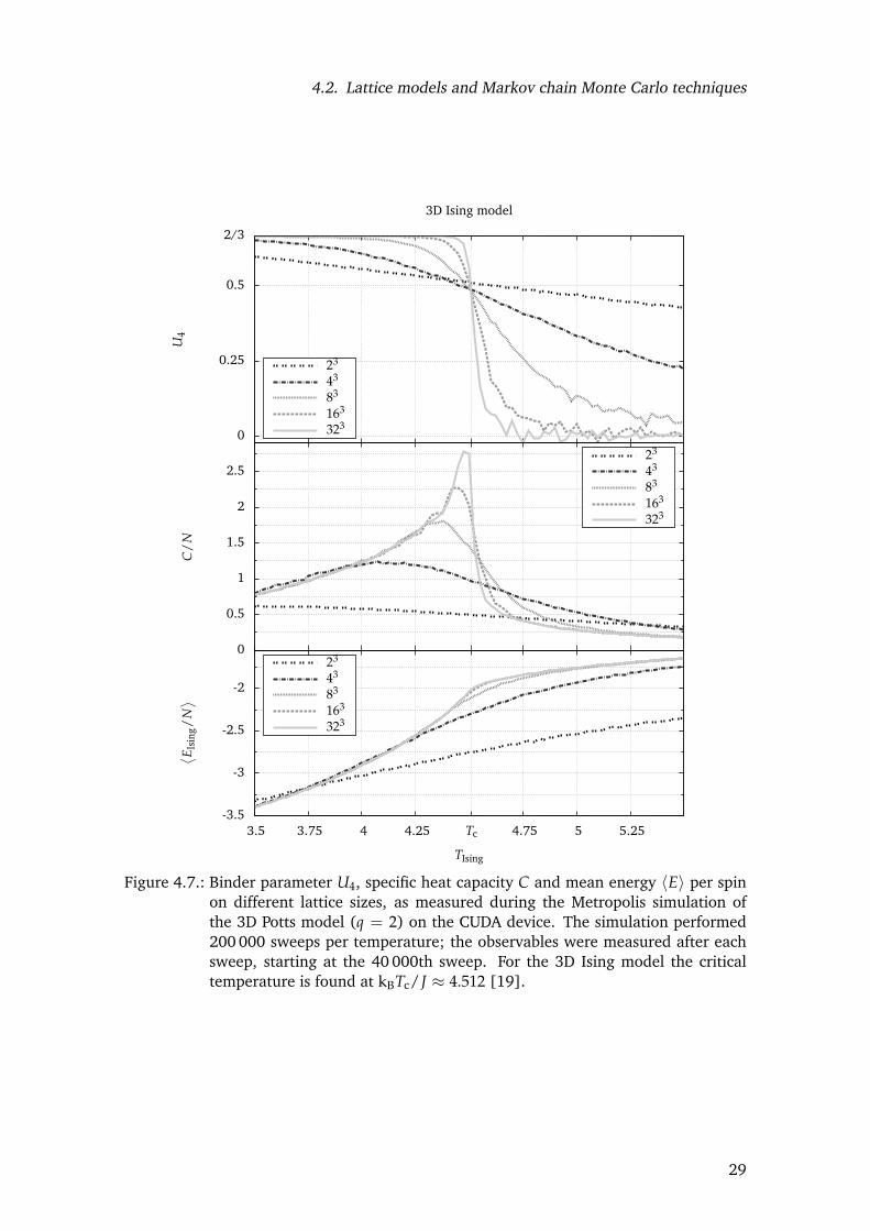
For the complete code listing please see the file potts.cu or section A.2 in the annex. Asimplified flowchart of the program is shown in figure 4.8. This implementation keepstrack of the spins by maintaining two lists of spin IDs: one array for the black spins, theother one for the white spins. The spin states themselves are stored in a third array, withthe array index corresponding to the spin ID. The spins are initialized on the CPU with arandom state (lines 149. . . 172).

For the simulation, the CUDA kernel function that carries out the Metropolis algorithm iscalled twice during each sweep (lines 270. . . 274). Once for all the black sites and oncefor all the white sites (fig. 4.4).

This ensures that only non-interacting spins are flipped simultaneously. Since the spinvalues are stored in a one-dimensional spin list and their neighbours are managed with a

23


1 2 2 1 2 3 3 1

2 2 1 1 1 3 3 1

3 3 1 3 2 2 3 2

0 2 3 3 2 2 1 0

1 3 3 3 2 2 1 2

2 2 3 1 2 3 3 0

3 1 1 1 1 3 0 3

1 3 3 2 1 1 2 2

Figure 4.3.: Checkerboard decomposition of an 8×8 spin lattice into two sets of non-interacting spins (black and white). The numbers denote the example spinstates from the lower left section of the 4-state Potts model lattice at T = 1.6in figure 4.2.

16×16 = 256 sites

−→ 1.

4 blocks · 32 threads per block = 128 threads

−→ 2.

4 blocks · 32 threads per block = 128 threads

Figure 4.4.: Checkerboard decomposition and assignment of the sites to blocks andthreads. In this example, the Metropolis algorithm for a lattice of 16×16sites is carried out in two parts. At first, a kernel function is called on theCUDA device to handle all the black sites. After the call is finished, anotherkernel carries out the Metropolis algorithm for all the white sites. Each threadis responsible for one (potential) spin flip.

simple neighbourhood table, there is no need to represent the actual lattice geometry onthe GPU. Each spin is assigned to a thread; they are distributed in such a way that eachblock takes care of a number of spins that is a multiple of 32 (the warp size).

Before the actual Metropolis algorithm starts, the energy of the sample lattice is calculatedonce on the CPU (lines 213. . . 223). To calculate the energy after spin flips have beenmade throughout the Metropolis algorithm, a kind of bookkeeping is introduced whichconsiders differences of the energy to the initial configuration. Whenever a spin is flipped,the resulting change in energy is recorded on a list. This minimizes the data transferbetween the host CPU and the CUDA device, since after each sweep only one energydifference per block needs to be transferred (lines 279. . . 286).

To verify the results from the CUDA simulation, the values for the mean energy 〈E〉(T)and the specific heat capacity C(T) are compared to the exact results derived from Beale’sexact solution [14] for the density of states Ω(E) of the two-dimensional Ising model(fig. 4.6).

The Ising model [15] is a spin model similar to the Potts model. Each spin on the lattice isin one of two possible states: si = ±1. For nearest-neighbour interaction 〈ij〉 the system’s

24


Hamiltonian is

HIsing = −J ∑〈ij〉

sisj + h ∑i

si . (4.6)

Again, J denotes the coupling energy and si the value of spin i. The system’s symmetrycan be broken with an external magnetic field h, but in this example we consider it to bezero: h = 0.

Due to this analogous nature, observables of the Potts model for two spin states (q = 2→si ∈ 0, 1) can be linked to the Ising model’s observables. We consider the temperatureT = 1/β, the mean energy 〈E〉(T) and the specific heat capacity C(T):

TIsing = 2TPotts , (4.7)

EIsing = 2EPotts + 2JN , (4.8)

CIsing = β2Ising

[〈E2

Ising〉 − 〈EIsing〉2]= β2

Potts[〈E2

Potts〉 − 〈EPotts〉2]= CPotts . (4.9)

The energy conversion depends on the number of spins N. The constant 2JN does notplay a role for the specific heat capacity C which is conceptually the energy’s variance.

Additionally, the Binder parameter U4 [16] has been measured for two-dimensional (fig. 4.6)and three-dimensional (fig 4.7) lattices. It is defined as

U4(T) = 1− 〈m(T)4〉3〈m(T)2〉2 (4.10)

and takes higher moments of the magnetization m into account. For the Ising model, themagnetization is the sum of all spin values:

m =MN

=1N

N

∑i=1

si . (4.11)

To calculate the magnetization, the spin values from the 2-state Potts model were remappedto the values of the Ising model:

sPotts = 0←→ sIsing = −1 , (4.12)

sPotts = 1←→ sIsing = +1 . (4.13)

25


4.2.4. Execution times

The most important aim of parallel processing is to save time. Therefore, it is useful tocompare the execution times of a program running on the CPU directly to the one runningon the CUDA device.

Two test systems have been used. The first was the compute cluster Grawp at the Institutefor Theoretical Physics (ITP) at the University of Leipzig, specifically one Intel Xeon E5520processor1 to measure the CPU computation times and an NVIDIA Tesla C10602 as a CUDAdevice.

The second test system was a ThinkPad T410 with an Intel Core i7 M620 CPU3 and anNVIDIA NVS3100M4 graphics card.

The parallel code has been rewritten to run within a single thread on a CPU. The CPUprogram was built using the C++ compiler from gcc 4.4.4 with O1 optimization for a64 bit x86 Linux architecture. The same parameters applied to the compilation of theCUDA version: NVIDIA’s nvcc 4.2 compiler uses gcc 4.4.4 for the C code.

The execution times were measured with the Linux time command, adding the times theprograms spent in user and kernel (sys) mode.

Each program was initialized with a random lattice and then ran a simulation at 45 dif-ferent temperatures (TIsing, 2D = 0.8 . . . 5.2 and TIsing, 3D = 2.3 . . . 6.7, both in steps of∆T = 0.1), carrying out 50 000 sweeps for each temperature.

The measured execution times are shown in table 4.2 along with the thread and blockarrangements. Figure 4.5 shows the same values on a logarithmic scale. The times aregiven in execution time per spin, in the following defined as

τ =total program execution timeNspins · Nsweeps · Ntemperatures

. (4.14)

Whenever possible, the number of threads per block was set to be a multiple of 32, thewarp size, to take advantage of block cycles. The optimal distribution of blocks and threadsper block depends on factors such as the amount of shared memory required per blockand the number of registers per thread. NVIDIA offers a multiprocessor occupancy calcu-lator [17] to help with the fine-tuning.

1Intel Xeon E5520, 2.27 GHz, 8 MB L3 cache, 4×256 KB L2 cache2NVIDIA Tesla C1060, 1.30 GHz clock rate, 240 CUDA Cores on 30 multiprocessors3Intel Core i7 M620, 3.0 GHz, 4 MB L3 cache, 2×256 KB L2 cache4NVIDIA NVS3100M, 1.47 GHz clock rate, 16 CUDA Cores on 2 multiprocessors

26


Grawp ThinkPadL blocks threads/block τCPU

1 τCUDA2 τCPU

3 τCUDA4

2D square 2 1 2 100.0 ns 7911.1 ns 57.8 ns 9133.3 ns4 1 8 94.4 ns 1922.2 ns 56.9 ns 2330.6 ns8 1 32 95.1 ns 527.1 ns 56.5 ns 672.9 ns

16 4 32 93.9 ns 133.2 ns 55.5 ns 178.0 ns32 16 32 94.7 ns 33.9 ns 55.4 ns 63.0 ns64 64 32 94.7 ns 10.7 ns 57.5 ns 35.9 ns

128 128 64 94.5 ns 5.3 ns 57.6 ns 28.1 ns256 256 128 94.5 ns 4.4 ns 64.0 ns 25.7 ns

3D cubic 2 1 4 105.6 ns 4011.1 ns 63.9 ns 4827.8 ns4 1 32 100.7 ns 559.7 ns 61.8 ns 706.3 ns8 8 32 101.6 ns 71.6 ns 60.4 ns 115.1 ns

16 64 32 101.4 ns 12.5 ns 60.4 ns 50.1 ns32 128 128 102.4 ns 6.7 ns 60.5 ns 40.4 ns

Table 4.2.: Execution time τ per spin of the single CPU and the CUDA implementationsfor the simulation of the Metropolis algorithm on the 2-state Potts model, asmeasured by the Linux time command. The measurements were taken on twodifferent test systems (see text for details).

4

10

25

50

100

250

500

1000

2500

5000

10000

22 42 82 162 322 642 1282 2562

τ[n

s/sp

in]

Number of spins N

2D Potts model

23 43 83 163 323

Number of spins N

3D Potts model

Xeon E5520Core i7 M620Tesla C1060NVS3100M

Figure 4.5.: Execution time τ per spin of the single CPU and the CUDA implementationsfor the simulation of the Metropolis algorithm on the 2-state Potts model, asmeasured by the time command. The values are listed in table 4.2. The timescales are the same for both graphs.

27


0

0.25

0.5

2/3

U4

2D Ising model

0

0.5

1

1.5

C/

N

-2

-1.5

-1

1.75 2 Tc 2.5 2.75 3 3.25

⟨ E Isi

ng/

N⟩

TIsing

2×24×48×816×1632×3264×64128×128256×256

2×24×48×816×16

2×24×48×816×16

Figure 4.6.: Binder parameter U4, specific heat capacity C and mean energy 〈E〉 per spinon different lattice sizes, as measured during the Metropolis simulation ofthe 2D Potts model (q = 2) on the CUDA device. In the diagrams for C and〈E〉, the points denote the measurements whereas the solid lines represent thevalues derived from Beale’s exact solution [14] for the density of states. Thesimulation performed 30 000 sweeps per temperature; the observables weremeasured after each sweep, starting at the 6 000th sweep. For the 2D Isingmodel the critical temperature is found at kBTc/J ≈ 2.269 [18].

28


0

0.25

0.5

2/3

U4

3D Ising model

0

0.5

1

1.5

2

2.5

C/

N

-3.5

-3

-2.5

-2

3.5 3.75 4 4.25 Tc 4.75 5 5.25

⟨ E Isi

ng/

N⟩

TIsing

23

43

83

163

323

23

43

83

163

323

23

43

83

163

323

Figure 4.7.: Binder parameter U4, specific heat capacity C and mean energy 〈E〉 per spinon different lattice sizes, as measured during the Metropolis simulation ofthe 3D Potts model (q = 2) on the CUDA device. The simulation performed200 000 sweeps per temperature; the observables were measured after eachsweep, starting at the 40 000th sweep. For the 3D Ising model the criticaltemperature is found at kBTc/J ≈ 4.512 [19].

29


CPU host program CUDA device kernel function

Random spin states:

uint spins[N]

Store spin IDs:

uint black[N/2]

uint white[N/2]

Calculate the system’s energy:H = −J ∑〈ij〉 δsisj

Copy data to CUDA device’s global memory:

seeds, spins, neighbors, white IDs, black IDs

Call kernel function for black spins:

runMetropolis(pBlackSpinIDs)

Spin’s ID depends on whether black or white

list of spin IDs has been given as parameter:

id = blockDim.x*blockIdx.x + threadIdx.x

spinID = spinIDs[id]

Energy difference for each thread stored as

array in shared memory for each block:

__shared__ int deltaE[N_THREADS_PER_BLOCK]

Propose spin flip; Metropolis criterion.

Record energy difference:∆E = Ebefore flip − Eafter flip

__syncthreads()

First thread in block sums up energy differences.

Call kernel function for white spins:

runMetropolis(pWhiteSpinIDs)

Same algorithm for white spins.

Evaluate energy differences→ E ≈ 〈E〉.

i < Nsweeps

Figure 4.8.: Simplified flowchart of the CUDA implementation of the Metropolis algorithmfor the Potts model. The spin values are stored in a one-dimensional array. Aneighbourhood table is used.

30

5. Conclusions

For small lattices (N < 256 spins) the parallel architecture of the CUDA devices cannotbe used efficiently. The multiprocessors carry out the Metropolis algorithm with too fewactive threads and their memory not optimally used. For bigger lattices the simulationsran up to a factor of 20 faster than on the system’s CPU.

Further optimizations usually include techniques that take advantage of the underlyinghardware. Momchil Ivanov [20] reports Metropolis update times that are up to a factorof 8 faster than in this work. This result is reached not only by the slightly better hard-ware, but among other techniques by an intelligent reordering of the spin arrays, takingadvantage of the GPU’s memory structure and read/write mechanisms.

The main focus of this work stayed on code simplicity and easy code portability. Thespeed comparison between CPU and GPU included the measurement of the energy aftereach sweep. For real-world scenarios even more observables will need to be evaluatedduring the simulation, increasing the amount of data that needs to be transferred fromthe GPU to the host system.

In the future, the speed advantage of GPUs over CPUs will probably increase further withrespect to higher clock rates and more processing cores. However, even if CPUs might notbe able to gain proportionally higher clock rates, their number of cores also tends to in-crease and their memory and thread management will yield further speed improvements.

The decision on whether to implement a simulation on a CPU or a GPU will depend onthe one hand on technical factors such as how much memory is needed per parallel entity,how much data needs to be transferred between the GPU and the host system and to whatdegree a model can be parallelized. On the other hand human factors also play a role, suchas how much time it will take to test the new implementations, to fine-tune the parametersfor optimal speeds, and even how long it will take to learn sophisticated programmingtechniques like CUDA C, the manufacturer-independent OpenCL, or the Message PassingInterface (MPI) intended for usage with many CPUs.

With deep knowledge of the hardware, simulations can usually be adapted to reach highefficiencies. Often, the drawback is a loss of universality and simplicity of the code. Graph-ics cards will play an important role when it comes to time-intensive computing tasks,especially in the scientific community where more and more people adopt parallel mech-anism for new projects and gain practical experience with this young technology.

31

A. Code listings

A.1. Conway’s Game of Life


3 #define ALIVE 14 #define DEAD 05

6 // world size in x and y direction:7 #define WX 168 #define WY 16 // 16*16 = 256 sites9 #define N WX*WY // number of sites

10

11 // Device function: get world array index from world coordinates12 __device__ unsigned getId(int x, int y)13 14 // periodic boundary conditions:15 while(x >= WX)16 x -= WX;17

18 while(x < 0)19 x += WX;20

21 while(y >= WY)22 y -= WY;23

24 while(y < 0)25 y += WY;26

27 return x + y * WX;28 29

30 // Kernel:31 __global__ void runConway(unsigned short* world, unsigned iterations)32 33 // get the world coordinate:34 int x = blockIdx.x * blockDim.x + threadIdx.x;35 int y = blockIdx.y * blockDim.y + threadIdx.y;36

37 // id in 1D array which represents the world:38 unsigned id = getId(x, y);39

40 // create a copy of the world in local shared memory:41 __shared__ unsigned short sites[N];42 sites[id] = world[id];43

44 // wait for all threads to finish copying:

33

A. Code listings

45 __syncthreads();46

47 // run the defined number of steps (iterations):48 for(unsigned i=0; i<iterations; i++)49 50 // determine new state by rules of Conway’s Game of Life:51 unsigned short state = sites[id];52 unsigned short newstate = state;53

54 // calculate number of alive neihbors:55 unsigned short aliveNeighbors = 0;56

57 for(short x_offset=-1; x_offset<=1; x_offset++)58 59 for(short y_offset=-1; y_offset<=1; y_offset++)60 61 if(x_offset != 0 || y_offset != 0) // don’t count itself62 63 unsigned neighborId = getId(x + x_offset, y + y_offset);64 aliveNeighbors += sites[neighborId];65 66 67 68

69 // decide about new state:70 if(state == ALIVE)71 72 if(aliveNeighbors < 2 || aliveNeighbors > 3)73 newstate = DEAD;74 else75 newstate = ALIVE;76 77 else // if DEAD78 79 if(aliveNeighbors == 3)80 newstate = ALIVE;81 82

83 // wait for all threads to determine new state:84 __syncthreads();85

86 // save spins in shared memory:87 sites[id] = newstate;88

89 // wait for all threads to copy new state to shared memory:90 __syncthreads();91 92

93 // copy spins back to global memory:94 world[id] = sites[id];95 96

97 // Host function (CPU Code)98 int main (int argc, char const* argv[])99

100 // matrix values:

34

A.1. Conway’s Game of Life

101 unsigned short world[N];102

103 // number of steps in Conway’s Game of Life:104 unsigned iterations = 3;105

106 // create dead world:107 for(unsigned i=0; i<N; i++)108 world[i] = 0;109

110 // set up a glider:111 world[1 + 0 * WX] = ALIVE; // 010000...112 world[2 + 1 * WX] = ALIVE; // 001000...113 world[0 + 2 * WX] = ALIVE; // 111000...114 world[1 + 2 * WX] = ALIVE; // 000000...115 world[2 + 2 * WX] = ALIVE; // ......116

117 // allocate memory on CUDA device:118 unsigned short* pDevWorld; // pointer to the data on the CUDA Device119 cudaMalloc((void**)&pDevWorld, sizeof(world));120

121 // copy data to CUDA device:122 cudaMemcpy(pDevWorld, &world, sizeof(world), cudaMemcpyHostToDevice);123

124 // set block and grid dimensions:125 dim3 blockSize(WX, WY);126 dim3 gridSize(1, 1, 1); // just 1 block for this easy example127

128 // execute kernel function on GPU:129 runConway<<<gridSize, blockSize>>>(pDevWorld, iterations);130

131 // copy data back from CUDA Device to ’data’ array:132 cudaMemcpy(&world, pDevWorld, sizeof(world), cudaMemcpyDeviceToHost);133

134 // free memory on the CUDA Device:135 cudaFree(pDevWorld);136

137 // output results:138 for(unsigned y=0; y<WY; y++)139 140 for(unsigned x=0; x<WX; x++)141 142 std::cout<<world[x + WX*y];143 144 std::cout<<"\n";145 146

147 return 0;148

35

A. Code listings

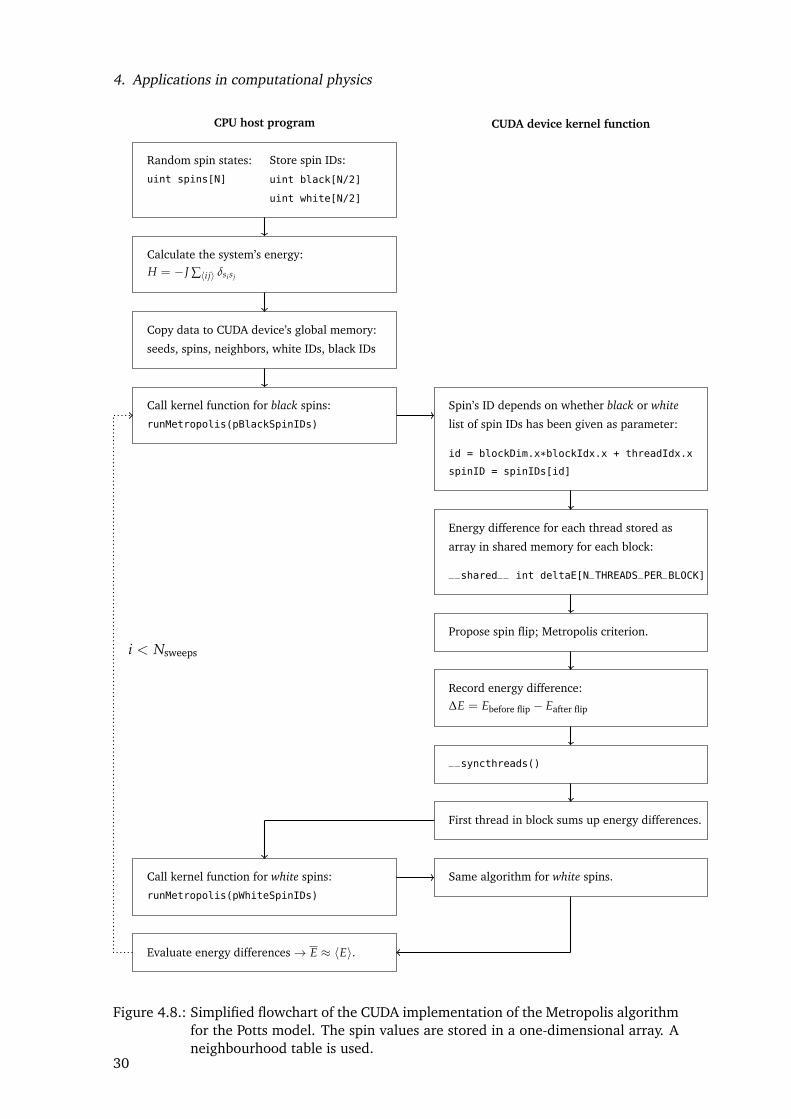
A.2. Metropolis algorithm for the Potts model


3 #define L 16 // lattice length; must be even number!4 #define D 2 // dimensions5 #define N 256 // number of spins on square lattice (N=L^D)6 #define Q 2 // number of Potts states7

8 #define N_SWEEPS 1000009

10 /* Distribute N/2 spins over threads and blocks:11 since we do "black" and "white" spins seperately, we only need half the threads:12 N_BLOCKS * N_THREADS_PER_BLOCK = N/2 */13 #define N_BLOCKS 4 // number of blocks14 #define N_THREADS_PER_BLOCK 32 // number of threads per block15

16

17 /**********************************18 * GPU RANDOM NUMBER GENERATION *19 **********************************/20

21 __device__ unsigned Tausworthe88(unsigned &z1, unsigned &z2, unsigned &z3)22 23 // Three-step generator with period 2^8824 unsigned b = (((z1 << 13) ^ z1) >> 19);25 z1 = (((z1 & 4294967294) << 12) ^ b);26

27 b = (((z2 << 2) ^ z2) >> 25);28 z2 = (((z2 & 4294967288) << 4) ^ b);29

30 b = (((z3 << 3) ^ z3) >> 11);31 z3 = (((z3 & 4294967280) << 17) ^ b);32

33 return z1 ^ z2 ^ z3;34 35

36 __device__ unsigned LCRNG(unsigned &z)37 38 const unsigned a = 1664525, c = 1013904223;39 return z = a * z + c;40 41

42 __device__ float TauswortheLCRNG(unsigned &z1, unsigned &z2, unsigned &z3, unsigned&z)

43 44 // combine both generators and normalize 0...2^32 to 0...145 return (Tausworthe88(z1, z2, z3) ^ LCRNG(z)) * 2.3283064365e-10;46 47

48

49 /******************************50 * GPU METROPOLIS ALGORITHM *51 ******************************/52

36


53 __global__ void runMetropolis(int *seeds, unsigned short* spins, unsigned*neighbors, unsigned* spinIdList, int* energyDifferences, float beta)

54 55 const unsigned id = blockDim.x*blockIdx.x + threadIdx.x;56

57 // spin id from list of black or white spins:58 const unsigned spinId = spinIdList[id];59

60 // get seed values:61 unsigned z1 = seeds[4*id ]; // Tausworthe seeds62 unsigned z2 = seeds[4*id + 1];63 unsigned z3 = seeds[4*id + 2];64 unsigned z = seeds[4*id + 3]; // LCRNG seed65

66 // energy differences for this block:67 __shared__ int deltaE[N_THREADS_PER_BLOCK];68 deltaE[threadIdx.x] = 0;69

70 unsigned short spinstate = spins[spinId]; // get spin state from DRAM71 unsigned short nb[2*D]; // neighbor states72

73 // get neighbor states:74 for(unsigned n=0; n<2*D; n++)75 nb[n] = spins[neighbors[2*D*spinId + n]];76

77 // propose random new spin state:78 unsigned short newstate = floor(TauswortheLCRNG(z1, z2, z3, z) * Q);79

80 // energy difference: E’-E81 int E_before = 0;82 int E_after = 0;83

84 for(unsigned short n=0; n<2*D; n++)85 86 if(spinstate == nb[n])87 E_before++;88

89 if(newstate == nb[n])90 E_after++;91 92

93 // acceptance probability:94 float dE = __int2float_rn(E_before - E_after);95 float pAccept = __expf(-beta*dE);96

97 if(TauswortheLCRNG(z1, z2, z3, z) <= pAccept)98 99 spins[spinId] = newstate; // flip spin

100 deltaE[threadIdx.x] = E_before - E_after; // note energy difference101 102

103 // store new seed values in DRAM:104 seeds[4*id ] = z1; // Tausworthe seeds105 seeds[4*id + 1] = z2;106 seeds[4*id + 2] = z3;107 seeds[4*id + 3] = z; // LCRNG seed

37

A. Code listings

108

109 __syncthreads();110

111 // sum up this block’s energy delta:112 if(threadIdx.x == 0)113 114 int blockEnergyDiff = 0;115 for(unsigned i=0; i<blockDim.x; i++)116 blockEnergyDiff += deltaE[i];117

118 energyDifferences[blockIdx.x] += blockEnergyDiff;119 120 121

122

123 /******************************124 * HOST FUNCTION (CPU PART) *125 ******************************/126

127 int main(int argc, char const *argv[])128 129 // each spin has value 0,..,Q-1130 unsigned short spins[N];131

132 // calculate lattice volume elements:133 unsigned volume[D];134 for(unsigned i=0; i<=D; i++)135 136 if(i == 0)137 volume[i] = 1;138 else139 volume[i] = volume[i-1] * L;140 141

142

143 /* Determine the "checkerboard color" (black or white) for each site and144 initialise lattice with random spin states: */145 unsigned w=0, b=0;146 unsigned white[N/2], black[N/2]; // store ids of white/black sites147

148 for(unsigned i=0; i<N; i++)149 150 // Sum of all coordinates even or odd? -> gives checkerboard color151 int csum = 0;152 for(int k=D-1; k>=0; k--)153 csum += ceil((i+1.0)/volume[k]) - 1;154

155 if((csum%2) == 0) // white156 157 white[w] = i;158 w++;159 160 else // black161 162 black[b] = i;163 b++;

38


164 165

166 // random spin state:167 spins[i] = floor(drand48() * Q);168 169

170

171 // neighborhood table:172 unsigned neighbors[2*D*N];173

174 // calculate neighborhood table:175 for(unsigned i=0; i<N; i++)176 177 unsigned short c=0;178

179 for(unsigned short dim=0; dim<D; dim++) // dimension loop180 181 for(short dir=-1; dir<=1; dir+=2) // two directions in each dimension182 183 // neighbor’s id in spin list:184 int npos = i + dir * volume[dim];185

186 // periodic boundary conditions:187 int test = (i % volume[dim+1]) + dir*volume[dim];188

189 if(test < 0)190 npos += volume[dim+1];191 else if(test >= volume[dim+1])192 npos -= volume[dim+1];193

194 neighbors[2*D*i + c] = npos;195 c++;196 197 198 199

200

201 // create 4 seed values for each thread:202 unsigned seeds[4*N/2];203 for(unsigned i=0; i<4*N/2; i++)204 205 seeds[i] = static_cast<unsigned>(4294967295 * drand48());206 207

208

209 // calculate energy (Potts model)210 int E = 0;211 for(unsigned i=0; i<N; i++)212 213 for(unsigned j=0; j<2*D; j++)214 215 if(spins[i] == spins[neighbors[2*D*i + j]])216 E--;217 218 219 E /= 2; // count each interaction only once

39

A. Code listings

220

221

222 // copy seeds to GPU:223 int *devPtrSeeds;224 cudaMalloc((void**)&devPtrSeeds, sizeof(seeds));225 cudaMemcpy(devPtrSeeds, &seeds, sizeof(seeds), cudaMemcpyHostToDevice);226

227 // copy spins to GPU:228 unsigned short *devPtrSpins;229 cudaMalloc((void**)&devPtrSpins, sizeof(spins));230 cudaMemcpy(devPtrSpins, &spins, sizeof(spins), cudaMemcpyHostToDevice);231

232 // copy neighborhood table to GPU:233 unsigned *devPtrNeighbors;234 cudaMalloc((void**)&devPtrNeighbors, sizeof(neighbors));235 cudaMemcpy(devPtrNeighbors, &neighbors, sizeof(neighbors),

cudaMemcpyHostToDevice);236

237 // copy white ids to GPU:238 unsigned *devPtrWhite;239 cudaMalloc((void**)&devPtrWhite, sizeof(white));240 cudaMemcpy(devPtrWhite, &white, sizeof(white), cudaMemcpyHostToDevice);241

242 // copy black ids to GPU:243 unsigned *devPtrBlack;244 cudaMalloc((void**)&devPtrBlack, sizeof(black));245 cudaMemcpy(devPtrBlack, &black, sizeof(black), cudaMemcpyHostToDevice);246

247 // each block calculates energy difference to initial state:248 int energyDifferences[N_BLOCKS];249 for(unsigned i=0; i<N_BLOCKS; i++)250 energyDifferences[i] = 0;251

252 int *devPtrEnergyDifferences;253 cudaMalloc((void**)&devPtrEnergyDifferences, sizeof(energyDifferences));254 cudaMemcpy(devPtrEnergyDifferences, &energyDifferences, sizeof(

energyDifferences), cudaMemcpyHostToDevice);255

256

257 int E_before_simulation = E;258 long long sum_E = 0;259 const float T = 1.25; // simulation temperature260

261 for(unsigned i=0; i<N_SWEEPS; i++)262 263 // White spins:264 runMetropolis<<<N_BLOCKS, N_THREADS_PER_BLOCK>>>(devPtrSeeds, devPtrSpins,

devPtrNeighbors, devPtrWhite, devPtrEnergyDifferences, 1.0f/T);265

266 // Black spins:267 runMetropolis<<<N_BLOCKS, N_THREADS_PER_BLOCK>>>(devPtrSeeds, devPtrSpins,

devPtrNeighbors, devPtrBlack, devPtrEnergyDifferences, 1.0f/T);268

269 // Sum up energy after a thermalization time for mean energy value:270 if(i > 0.2*N_SWEEPS)271

40


272 // get energy changes from the GPU:273 cudaMemcpy(&energyDifferences, devPtrEnergyDifferences, sizeof(

energyDifferences), cudaMemcpyDeviceToHost);274

275 E = E_before_simulation;276 for(unsigned t=0; t<N_BLOCKS; t++) // take energy changes into account277 E += energyDifferences[t];278

279 sum_E += E;280 281 282

283 cudaFree(devPtrSeeds);284 cudaFree(devPtrSpins);285 cudaFree(devPtrNeighbors);286 cudaFree(devPtrWhite);287 cudaFree(devPtrBlack);288 cudaFree(devPtrEnergyDifferences);289

290 return 0;291

41

B. Glossary

Block An array of threads that will run on the CUDA device. The threads are identifiedby one-, two- or three-dimensional coordinates within the block.

CPU Central Processing Unit, the main processor on a computer’s mainboard.

Compute Capability A revision number that guarantees a certain set of features, specifi-cations and instructions for all CUDA devices that carry this number. For details, seeAppendix G in the NVIDIA CUDA C Programming Guide [1].

CUDA Core scalar processor that forms part of a multiprocessor. Each multiprocessorcomes with several CUDA cores for parallel execution.

CUDA Device In this document, a device (usually a graphics card) that supports CUDAinstructions.

Device In CUDA terms, the device is always the CUDA Device. It executes the devicecode.

Global memory The main memory on the graphics card which each multiprocessor andthe CPU host have access to.

Grid An array of blocks of threads. The blocks are identified by one- or two-dimensionalcoordinates within the grid.

GPU Graphics Processing Unit, hardware designed for highly parallel graphics calcula-tions.

Host In CUDA terms, the host is the system that hosts the GPU. Host code runs on theCPU and host memory is the host system’s RAM.

Kernel A function that will be executed in many threads on the CUDA device.

Multiprocessor (MP) Processing unit on the graphics card that houses a certain numberof scalar CUDA cores, memory, and special purpose processors. Each CUDA devicecomes with a certain number of MPs.

Shared memory Local memory on each multiprocessor. Access to this memory is re-stricted to the components of a multiprocessor.

Thread Smallest unit of a parallel program. Usually many threads execute the sameinstructions simultaneously, i.e. work on the same problem with different data.

Warp size The number of threads a multiprocessor treats at once. Up to the date of thisdocument, the warp size is 32 for all CUDA devices (compute capability 1.0 through3.0)

43

Bibliography

[1] NVIDIA CUDA C Programming Guide, 2011.http://developer.nvidia.com/cuda-downloads.

[2] NVIDIA CUDA C Getting Started Guide, 2011.http://developer.nvidia.com/cuda-downloads.

[3] NVIDIA GPU Computing SDK.http://developer.nvidia.com/gpu-computing-sdk.

[4] Martin Gardner. Mathematical Games: The fantastic combinations of John Conway’snew solitaire game “life”. Scientific American, pages 120–123, October 1970.

[5] Makoto Matsumoto and Takuji Nishimura. Mersenne twister: a 623-dimensionallyequidistributed uniform pseudo-random number generator. ACM Transactions onModeling and Computer Simulation, 8(1):3–30, January 1998.

[6] Tobias Preis, Peter Virnau, Wolfgang Paul, and Johannes J. Schneider. GPU acceler-ated Monte Carlo simulation of the 2D and 3D Ising model. Journal of ComputationalPhysics, 228(12):4468–4477, July 2009.

[7] Martin Weigel. Simulating spin models on GPU. Computer Physics Communications,182(9):1833–1836, September 2011.

[8] Lee Howes and David Thomas. GPU Gems 3, Chapter 37: Efficient RandomNumber Generation and Application Using CUDA. Technical report, http://http.developer.nvidia.com/GPUGems3/gpugems3_ch37.html, 2011.

[9] Pierre L’Ecuyer. Maximally equidistributed combined Tausworthe generators. Math-ematics of Computation, 65(213):203–214, January 1996.

[10] J. Ashkin and E. Teller. Statistics of Two-Dimensional Lattices with Four Components.Physical Review, 64(5-6):178–184, September 1943.

[11] R. B. Potts and C. Domb. Some generalized order-disorder transformations. Math-ematical Proceedings of the Cambridge Philosophical Society, 48(01):106, October1952.

[12] Nicholas Metropolis, Arianna W. Rosenbluth, Marshall N. Rosenbluth, Augusta H.Teller, and Edward Teller. Equation of State Calculations by Fast Computing Ma-chines. The Journal of Chemical Physics, 21(6):1087, 1953.

[13] Lars Onsager. Reciprocal Relations in Irreversible Processes. I. Physical Review,37(4):405–426, February 1931.

[14] Paul Beale. Exact Distribution of Energies in the Two-Dimensional Ising Model. Phys-ical Review Letters, 76(1):78–81, January 1996.

[15] Ernst Ising. Beitrag zur Theorie des Ferromagnetismus. Zeitschrift für Physik,31(1):253–258, February 1925.

45

http://developer.nvidia.com/cuda-downloads

http://developer.nvidia.com/cuda-downloads

http://developer.nvidia.com/gpu-computing-sdk

http://http.developer.nvidia.com/GPUGems3/gpugems3_ch37.html

http://http.developer.nvidia.com/GPUGems3/gpugems3_ch37.html

Bibliography

[16] Kurt Binder. Finite size scaling analysis of Ising model block distribution functions.Zeitschrift für Physik B Condensed Matter, 43(2):119–140, June 1981.

[17] CUDA Occupancy Calculator, NVIDIA Corporation.http://developer.nvidia.com/cuda/nvidia-gpu-computing-documentation.

[18] Lars Onsager. Crystal Statistics. I. A Two-Dimensional Model with an Order-DisorderTransition. Physical Review, 65(3-4):117–149, February 1944.

[19] A L Talapov and H W J Blöte. The magnetization of the 3D Ising model. Journal ofPhysics A: Mathematical and General, 29(17):5727–5733, September 1996.

[20] Momchil Ivanov. How fast are local Metropolis updates for the Ising model on agraphics card. In Mathias Winkel, editor, Guest Student Programme 2011, pages35–45. Forschungszentrum Jülich, 2011.

46

http://developer.nvidia.com/cuda/nvidia-gpu-computing-documentation

A short guide to CUDA C - tasty orange

Documents

Transcript of A short guide to CUDA C - tasty orange