ASYMPTOTIC APPROXIMATION OF THE SOLUTION OF THELAPLACE EQUATION IN A DOMAIN WITH HIGHLY

OSCILLATING BOUNDARY∗

Y. AMIRAT† , O. BODART‡ , U. DE MAIO§ , AND A. GAUDIELLO¶

ResumeOn etudie le comportement asymptotique de la solution de l’equation de Laplace dans un

domaine dont une partie de la frontiere est fortement oscillante. La motivation de ce travail

est l’etude d’un ecoulement longitudinal dans un domaine infini borne inferieurement par

une paroi et superieurement par une paroi rugueuse. Cette derniere est un plan recouvert

d’asperites periodiques dont la taille depend d’un petit parametre ε. On fait l’hypothese de

rugosite forte, a savoir que la hauteur des asperites reste constante. A l’aide d’un correcteur

de couche limite, on obtient une approximation non oscillante de la solution qui est d’ordre

ε3/2) en norme H1.

AbstractWe study the asymptotic behavior of the solution of the Laplace equation in a domain, a

part of which boundary is highly oscillating. The motivation comes from the study of a

longitudinal flow in an infinite horizontal domain bounded at the bottom by a wall and at

the top by a rugose wall. The latter is a plane covered with periodic asperities which size

depends on a small parameter ε > 0. The assumption of sharp asperities is made, that is the

height of the asperities is fixed. Using a boundary layer corrector, we derive and analyze a

nonoscillating approximation of the solution at order O(ε3/2) for the H1-norm.

Classification MSC : 35B40, 35C20, 35J05

∗This work is partially supported by the C.N.R. Project “Agenzia 2000”.†Laboratoire de Mathematiques Appliquees, CNRS (UMR 6620), Universite Blaise Pascal

(Clermont-Ferrand 2), 63177 Aubiere cedex,France (amirat@math.univ-bpclermont.fr).‡Laboratoire de Mathematiques Appliquees, CNRS (UMR 6620), Universite Blaise Pascal

(Clermont-Ferrand 2), 63177 Aubiere cedex,France (obodart@math.univ-bpclermont.fr).§Dipartimento di Matematica e Applicazioni “R. Caccioppoli”, Universita di Napoli “Federico

II”, Complesso Monte S. Angelo, via Cintia, 80126 Napoli, Italy (udemaio@unina.it).¶Dipartimento di Automazione, Elettromagnetismo, Ingegneria dell’Informazione e Matem-

atica Industriale, Universita di Cassino, via G. Di Biasio 43, 03043 Cassino (FR), Italy,(gaudiell@unina.it ).

1

1. Introduction. Boundary-value problems involving oscillating boundaries orinterfaces frequently arise when modelling problems in industrial applications, suchas flows over rough walls, electromagnetic waves in a region containing a rough inter-face, elastic bodies containing a rough interface. The mathematical analysis of theseproblems consists in studying the large scale behavior of the solution. The goal isto determine effective boundary conditions, or to construct accurate and numericallyimplementable asymptotic approximations. The main difficulty comes from the pres-ence of boundary layers near the rough region, which effects on correctors or errorestimates have to be taken into account. In the present paper we consider a boundary-value problem for the Laplace equation, arising from the study of a laminar flow overa rough wall.

Let us consider a viscous fluid in an infinite horizontal domain limited at thebottom by a wall P and at the top by a rough wall Rε. We assume that P movesat a constant horizontal velocity γ = (γ′, 0), γ′ ∈ R2, and that Rε is at rest. Thelatter is assumed to consist of a plane wall covered with periodic asperities which sizedepends on a small parameter ε > 0, and with a fixed height. Let 0 < ai < bi < li,i = 1, 2, S = (0, l1)× (0, l2), S = (a1, b1)× (a2, b2), Sε = εS, Sε = εS, and ηε be theSε-periodic function defined on Sε by

ηε (x′) =

l3 if x′ ∈ Sε\Sε,

l′3 if x′ ∈ Sε,

with l′3 > l3 > 0, and x′ = (x1, x2) . The domain of the flow is

Oε =(x′, x3) ∈ R3 : x′ ∈ R2, b(x′) < x3 < ηε (x′)

,

where b is a smooth and S-periodic function on R2 such that b(x′) < l3 in R2. Thedomain Oε is bounded at the bottom by

P =(x′, x3) ∈ R3 : x′ ∈ R2, x3 = b (x′)

,

and at the top by Rε = ∂Oε\O, where ∂Oε denotes the boundary of Oε. The profileof the asperities is then comb shaped. Throughout the paper, we will assume that1/ε ∈ N so that ηε is also periodic with period l1. Thus, Oε can be viewed asgenerated by periodic translations of the bounded domain

x ∈ R3 : x′ ∈ S, b(x′) < x3 < ηε (x′)

.

The velocity vε = (vε1, vε2, vε3) and the pressure pε of the fluid satisfy the stationaryNavier-Stokes equations

−ν∆vε + (vε · ∇) vε +∇pε = 0 in Oε,∇ · vε = 0 in Oε,vε = 0 on Rε,vε = γ on P,

(1.1)

and they are assumed to be periodic with respect to x1 and x2, with periods l1 andl2, respectively. Here ν > 0 denotes the viscosity. Suppose now that γ = (0, g, 0) andthat the functions b and ηε do not depend on x2, i.e. b = b(x1) and ηε = ηε(x1),b being a smooth function on R, l1-periodic, and ηε being the εl1-periodic functiondefined on (0, εl1) by

ηε(x1) =

l′3 if x1 ∈ (εa1,εb1),l3 if x1 ∈ (0, εl1)\(εa1,εb1).

(1.2)

2

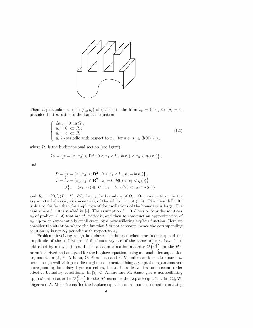
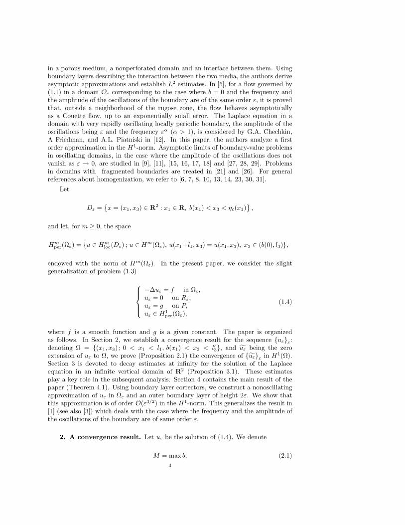
Then, a particular solution (vε, pε) of (1.1) is in the form vε = (0, uε, 0) , pε = 0,provided that uε satisfies the Laplace equation

∆uε = 0 in Ωε,uε = 0 on Rε,uε = g on P,uε l1-periodic with respect to x1, for a.e. x3 ∈ (b (0) , l3) ,

(1.3)

where Ωε is the bi-dimensional section (see figure)

Ωε =x = (x1,x3) ∈ R2 : 0 < x1 < l1, b(x1) < x3 < ηε (x1)

,

and

P =x = (x1, x3) ∈ R2 : 0 < x1 < l1, x3 = b(x1)

,

L =x = (x1, x3) ∈ R2 : x1 = 0, b(0) < x3 < η (0)

∪x = (x1, x3) ∈ R2 : x1 = l1, b(l1) < x3 < η (l1)

,

and Rε = ∂Ωε\ (P ∪ L) , ∂Ωε being the boundary of Ωε. Our aim is to study theasymptotic behavior, as ε goes to 0, of the solution uε of (1.3). The main difficultyis due to the fact that the amplitude of the oscillations of the boundary is large. Thecase where b = 0 is studied in [4]. The assumption b = 0 allows to consider solutionsuε of problem (1.3) that are εl1-periodic, and then to construct an approximation ofuε, up to an exponentially small error, by a nonoscillating explicit function. Here weconsider the situation where the function b is not constant, hence the correspondingsolution uε is not εl1-periodic with respect to x1.

Problems involving rough boundaries, in the case where the frequency and theamplitude of the oscillations of the boundary are of the same order ε, have beenaddressed by many authors. In [1], an approximation at order O

(ε

32

)for the H1-

norm is derived and analyzed for the Laplace equation, using a domain decompositionargument. In [2], Y. Achdou, O. Pironneau and F. Valentin consider a laminar flowover a rough wall with periodic roughness elements. Using asymptotic expansions andcorresponding boundary layer correctors, the authors derive first and second ordereffective boundary conditions. In [3], G. Allaire and M. Amar give a nonoscillatingapproximation at order O

(ε

32

)for the H1-norm for the Laplace equation. In [22], W.

Jager and A. Mikelic consider the Laplace equation on a bounded domain consisting3

in a porous medium, a nonperforated domain and an interface between them. Usingboundary layers describing the interaction between the two media, the authors deriveasymptotic approximations and establish L2 estimates. In [5], for a flow governed by(1.1) in a domain Oε corresponding to the case where b = 0 and the frequency andthe amplitude of the oscillations of the boundary are of the same order ε, it is provedthat, outside a neighborhood of the rugose zone, the flow behaves asymptoticallyas a Couette flow, up to an exponentially small error. The Laplace equation in adomain with very rapidly oscillating locally periodic boundary, the amplitude of theoscillations being ε and the frequency εα (α > 1), is considered by G.A. Chechkin,A Friedman, and A.L. Piatniski in [12]. In this paper, the authors analyze a firstorder approximation in the H1-norm. Asymptotic limits of boundary-value problemsin oscillating domains, in the case where the amplitude of the oscillations does notvanish as ε → 0, are studied in [9], [11], [15, 16, 17, 18] and [27, 28, 29]. Problemsin domains with fragmented boundaries are treated in [21] and [26]. For generalreferences about homogenization, we refer to [6, 7, 8, 10, 13, 14, 23, 30, 31].

Let

Dε =x = (x1, x3) ∈ R2 : x1 ∈ R, b(x1) < x3 < ηε(x1)

,

and let, for m ≥ 0, the space

Hmper(Ωε) = u ∈ Hm

loc(Dε) ; u ∈ Hm(Ωε), u(x1+l1, x3) = u(x1, x3), x3 ∈ (b(0), l3),

endowed with the norm of Hm(Ωε). In the present paper, we consider the slightgeneralization of problem (1.3)

−∆uε = f in Ωε,uε = 0 on Rε,uε = g on P,uε ∈ H1

per(Ωε),

(1.4)

where f is a smooth function and g is a given constant. The paper is organizedas follows. In Section 2, we establish a convergence result for the sequence uεε:denoting Ω = (x1, x3) ; 0 < x1 < l1, b(x1) < x3 < l′3, and uε being the zeroextension of uε to Ω, we prove (Proposition 2.1) the convergence of uεε in H1(Ω).Section 3 is devoted to decay estimates at infinity for the solution of the Laplaceequation in an infinite vertical domain of R2 (Proposition 3.1). These estimatesplay a key role in the subsequent analysis. Section 4 contains the main result of thepaper (Theorem 4.1). Using boundary layer correctors, we construct a nonoscillatingapproximation of uε in Ωε and an outer boundary layer of height 2ε. We show thatthis approximation is of order O(ε3/2) in the H1-norm. This generalizes the result in[1] (see also [3]) which deals with the case where the frequency and the amplitude ofthe oscillations of the boundary are of same order ε.

2. A convergence result. Let uε be the solution of (1.4). We denote

M = max b, (2.1)4

and

Ω+ε = (x1,x3) ∈ Ωε : l3 < x3 < l′3 ,

Ω+ = (0, l1)× (l3, l′3) ,

Ω− =(x1,x3) ∈ R2 : x1 ∈ (0, l1) , b (x1) < x3 < l3

,

Σ = (0, l1)× l3 ,

Ω = Ω− ∪ Ω+ ∪ Σ.

In the sequel we will use the spaces Hmper(Ω) and Hm

per(Ω−) (for m ≥ 0), the definition

is similar to that of Hmper(Ωε) given in the previous section. The only regularity

assumptions we make here are that b is Lipschitz-continuous and f ∈ L2(Ω). Remarkthat

χΩ+ε

b1 − a1

l1weakly- ? in L∞

(Ω+

), (2.2)

where χΩ+ε

denotes the characteristic function of Ω+ε . To describe the limit problem,

as ε → 0, of problem (1.4), we introduce the function

u =

0 in Ω+,u− in Ω−,

(2.3)

where u− is the unique solution of the following problem:

−∆u− = f in Ω−,u− = 0 on Σ,u− = g on P,u− ∈ H1

per (Ω−) .

(2.4)

Let uε be the zero extension to Ω of uε. The following convergence result holds:Proposition 2.1. Let uε be the solution of problem (1.4) and let u be the function

defined in (2.3), (2.4). Then

uε → u strongly in H1(Ω). (2.5)

Proof. Let s ∈ C2 (R) be such that

s(t) =

0 if t >M + l3

2,

1 if t <3M + l3

4,

where M is given in (2.1), and let h(x1, x3) = gs(x3). Choosing uε − h as a testfunction in problem (1.4), we get

∫

Ωε

∇uε (∇uε −∇h) dx =∫

Ωε

f (uε − h) dx. (2.6)

5

Applying the Young inequality and the Poincare inequality, we have∫

Ωε

|∇uε|2 dx ≤ α

∫

Ωε

|∇uε|2 dx +1α

∫

Ω−|∇h|2 dx

+αc

∫

Ωε

|∇uε|2 dx +1α

∫

Ω

f2dx +∫

Ω−fh dx,

for any α > 0, where c is a constant independent of ε and α, and consequently,

(∫

Ωε

|∇uε|2) 1

2

dx ≤ c,

where c is a constant independent of ε. Then, by virtue of the Poincare inequality, thesequence uεε is bounded in H1(Ω). Therefore, up to a subsequence, not relabelledfor convenience, there exists a function u ∈ H1

per(Ω) (possibly depending on thesubsequence) such that u = g on P and

uε u weakly in H1 (Ω) ,uε → u strongly in L2 (Ω) .

(2.7)

Moreover, since

uε = uε χΩ+ε

in Ω+,

from (2.7) and (2.2), it follows that

u = 0 in Ω+. (2.8)

On the other hand, letting ε go to 0 in (1.4) with test functions ϕ ∈ C∞ (Ω−) suchthat ϕ is l1-periodic with respect to x1 for a.e. x3 ∈ (b (0) , l3), ϕ|P = 0 and ϕ|Σ = 0,it follows from (2.7) that u|Ω− solves problem (2.4). Since this problem admits aunique solution, convergences (2.7) hold for the whole sequence. To obtain the strongconvergence (2.5), by virtue of (2.7) and (2.8), it is enough to prove that

limε→0

‖∇uε‖(L2(Ω))2 = ‖∇u‖(L2(Ω−))2 . (2.9)

Relations (2.6), (2.7) and (2.8) provide that

limε→0

∫

Ω

|∇uε|2 dx = limε→0

(∫

Ω

∇uε∇h dx +∫

Ω

f (uε − h) dx

)

=∫

Ω−∇u∇h dx +

∫

Ω−f (u− h) dx.

(2.10)

Finally, choosing u− h as a test function in problem (2.4), it follows that∫

Ω−|∇u|2 dx =

∫

Ω−∇u∇h dx +

∫

Ω−f (u− h) dx. (2.11)

The convergence (2.9) is then obtained by comparing (2.10) with (2.11).6

3. Decay estimates. The asymptotic approximation of uε will involve the so-lution of the Laplace equation in an infinite vertical domain of R2. Let Λ+ =(a1, b1)× (0, +∞), Λ− = (0, l1)× (−∞, 0) and ψ± be the functions defined by

ψ+ ∈ H1(Λ+),ψ− ∈ H1

loc,per(Λ−), ∇ψ− ∈ L2(Λ−), (3.1)

∆ψ± = 0 in Λ±,ψ+ = 0 on ∂Λ+\Γ,ψ− = 0 on ((0, a1) ∪ (b1,l1))× 0 ,ψ+ = ψ− on Γ,∂ψ+

∂y3=

∂ψ−

∂y3+ 1 on Γ,

(3.2)

where Γ = (a1, b1) × 0. Here ψ− ∈ H1loc,per(Λ

−) means ψ− ∈ H1per(Λ

′) for anybounded domain Λ′ ⊂ Λ−. We denote by β the mean of ψ− over an horizontal sectionof Λ−:

β =1l1

∫ l1

0

ψ− (y1,−δ) dy1, ∀δ ∈ (0, +∞). (3.3)

The following result is proved in [4]:Proposition 3.1. Problem (3.1), (3.2) admits a unique solution. Moreover:

(i) the constant β is independent of δ ;(ii) for any α ∈ N2 and for any δ ∈ (0,+∞), there exists a constant cα,δ such

that

|∂αψ+(y1, y3)| ≤ cα,δ e−cy3 , ∀ (y1, y3) ∈ (a1, b1)× (δ,+∞) ;

(iii) for any α ∈ N2 and for any δ ∈ (0, +∞), there exists a constant cα,δ suchthat

|∂α(ψ− − β)(y1, y3)| ≤ cα,δ ecy3 , ∀ (y1, y3) ∈ (0, l1)× (−∞,−δ).

The above estimates are of the so-called de Saint-Venant type. The first is provedby means of Tartar’s lemma (see [25], pp. 49–58) ; see also [24]. The second is provedby adapting the proof of the first one. Let us remark that (3.1) and Proposition 3.1provide that ψ− − β ∈ H1

per(Λ−).

Proposition 3.1 implies the following result:Corollary 3.2. Let ψ± be the functions satisfying (3.1), (3.2). Then, there

exists two positive constants c and C, independent of ε, such that∫

Ω+ε

∣∣∣∣ψ+

(x1

ε,x3 − l3

ε

)∣∣∣∣2

dx ≤ C ε,

∫

Ω−

∣∣∣∣ψ−(

x1

ε,x3 − l3

ε

)− β

∣∣∣∣2

dx ≤ C ε,

∫

Ωε\Bε

∣∣∣∣∇(

ψ

(x1

ε,x3 − l3

ε

))∣∣∣∣2

dx ≤ C e−cε ,

where Bε = (0, l1) × (l3 − ε, l3 + ε), and ψ is the function defined by ψ = ψ− in Λ−

and ψ = ψ+ in Λ+.7

4. A corrector result. To build a corrector for the solution uε of problem (1.4),we need more regularity on the solution u− of problem (2.4). We then assume thefollowing regularity for f and b:

f ∈ H4per(Ω

−) ∩ L2(Ω), b ∈ H6per(0, l1). (4.1)

Let O− =(x1, x3) ∈ R2 : x1 ∈ R, b(x1) < x3 < l3

. The extension of u− to O− by

l1-periodicity is a solution in H1per(Ω

−) of−∆u− = f in O−,u− = 0 on R× l3,u− = g on (x1, b(x1)) : x1 ∈ R .

Using standard regularity results, see [19, 20], we then have

u− ∈ H6per

(Ω−

) ⊂ C4(Ω−

). (4.2)

Let now w be the function defined by

w =

0 in Ω+,w− in Ω−,

(4.3)

where w− is the unique solution in H1per(Ω

−) of

∆w− = 0 in Ω−,

w− = β∂u−

∂x3on Σ,

w− = 0 on P,

(4.4)

where u− is the solution of problem (2.4) and β is defined by (3.3). Let us point outthat, due to assumptions (4.1),

w− ∈ C3(Ω−). (4.5)

Indeed, the functions w− and u− being extended by l1-periodicity to O−, it followsthat w− is the solution in H1

per(Ω−) of

−∆w− = 0 in O−,

w− = β∂u−

∂x3on R× l3,

w− = 0 on (x1, b(x1)) : x1 ∈ R.

Due to (4.2), we have∂u−

∂x3∈ H5

per(Ω−), and consequently, w− ∈ H5

per(Ω−) ⊂ C3(Ω−).

This section is devoted to prove the following result.Theorem 4.1. Assume (4.1). Let uε be the solution of problem (1.4), u be

defined by (2.3), (2.4) and w by (4.3), (4.4). Then, there exists a positive constant c,independent of ε, such that

‖uε − u‖H1(Ωε\Bε)≤ c ε, (4.6)

for ε small enough, where Bε = (0, l1) × (l3 − ε, l3 + ε). If in addition f = 0 in Ω+,there exists a positive constant c, independent of ε, such that

‖uε − u− εw‖H1(Ωε\Bε) ≤ c ε32 , (4.7)

8

for ε small enough.To prove Theorem 4.1 we need to introduce some auxiliary functions. Let τε be

the function defined by

τε =

τ+ε = uε − εw+

ε − ε∂u−

∂x3(x1, l3)ψ+

(x1

ε,x3 − l3

ε

)in Ω+

ε ,

τ−ε = uε − u− − εw−ε −ε∂u−

∂x3(x1, l3)

(ψ−

(x1

ε,x3 − l3

ε

)− β

)in Ω−,

(4.8)and ρε be the function defined by

ρε =

ρ+ε = w+

ε − ε∂w−

∂x3(x1, l3) ψ+

(x1

ε,x3 − l3

ε

)in Ω+

ε ,

ρ−ε = w−ε − w− −ε∂w−

∂x3(x1, l3) ψ−

(x1

ε,x3 − l3

ε

)in Ω−,

(4.9)

where uε is the solution of problem (1.4), u− is the solution of problem (2.4), w− thesolution of problem (4.4), ψ± are the functions defined by (3.1), (3.2) and w±ε arefunctions in H1(Ω+) and H1

per(Ω−) respectively, satisfying

∆w+ε = 0 in Ω+

ε ,∆w−ε = 0 in Ω−,w+

ε = 0 on Rε\Σ,

w−ε = β∂u−

∂x3on Rε ∩ Σ,

w−ε = 0 on P,

w+ε = w−ε − β

∂u−

∂x3on Σ\Rε,

∂w+ε

∂x3=

∂w−ε∂x3

on Σ\Rε,

(4.10)

β being defined by (3.3). Theorem 4.1 will be an immediate consequence of the twofollowing propositions.

Proposition 4.2. Assume (4.1). Let τε be the function defined by (4.8). Then,there exists a positive constant c, independent of ε, such that

‖τε‖H1(Ωε) ≤ c ε, (4.11)

and, if f = 0 in Ω+,

‖τε‖H1(Ωε) ≤ c ε32 , (4.12)

for ε small enough.Proposition 4.3. Assume (4.1). Let ρε be the function defined by (4.9). Then,

there exists a positive constant c, independent of ε, such that

‖ρε‖H1(Ωε) ≤ c ε, (4.13)

for ε small enough.Proof of Proposition 4.2. Obviously, τ+

ε ∈ H1(Ω+ε ) and τ−ε ∈ H1(Ω−). Due to

the boundary conditions of uε, u, ψ± and w±ε , the functions τ+ε and τ−ε have the same

9

trace on Ω+ε ∩Ω−. Consequently, τε ∈ H1 (Ωε) . Moreover, τε is l1-periodic with respect

to x1 for a.e. x3 ∈ (b (0) , l3) and τε = 0 on Rε\ (x1, l′3) : x1 ∈ (0, l1) . Furthermore,

from the jump conditions in (3.2) and in (4.10) it follows that the normal derivativesof τ+

ε and τ−ε on Ω+ε ∩Ω− are opposite as elements of H− 1

2

(Ω+

ε ∩ Ω−)

. Consequently,∆τε is weakly defined in Ωε by

∆τε =

−ε∂3u−

∂x21∂x3

(x1, l3)ψ+

(x1

ε,x3 − l3

ε

)+

−2ε∂2u−

∂x1∂x3(x1, l3)

∂

x1

(ψ+

(x1

ε,x3 − l3

ε

))− f in Ω+

ε ,

−ε∂3u−

∂x21∂x3

(x1, l3)(

ψ−(

x1

ε,x3 − l3

ε

)− β

)+

−2ε∂2u−

∂x1∂x3(x1, l3)

∂

x1

(ψ−

(x1

ε,x3 − l3

ε

)− β

)in Ω−.

(4.14)Since

τε|P = −ε∂u−

∂x3(x1, l3)

(ψ−

(x1

ε,b (x1)− l3

ε

)− β

),

τε|Rε∩((0,l1)×l′3)= −ε

∂u−

∂x3(x1, l3) ψ+

(x1

ε,l′3 − l3

ε

),

setting

τ1ε (x1, x3) = −ε

∂u−

∂x3(x1, l3)

(ψ−

(x1

ε,b (x1)− l3

ε

)− β

)m1(x3) in Ωε,

τ2ε (x1, x3) = −ε

∂u−

∂x3(x1, l3)ψ+

(x1

ε,l′3 − l3

ε

)m2(x3) in Ωε,

where m1, m2 ∈ C2(R; [0, 1]) and

m1(t) =

0 if t >M + l3

2,

1 if t <3M + l3

4,

, m2(t) =

1 if t >l3 + l′3

2,

0 if t <3l3 + l′3

4,

(4.15)

M being defined by (2.1), it results that τε − τ1ε − τ2

ε ∈ H1per (Ωε), and vanishes on

10

Rε ∪ P. Then, multiplying (4.14) by τε − τ1ε − τ2

ε and integrating on Ωε, it follows∫

Ωε

|∇τε|2 dx

=∫

Ω−∇τε∇τ1

ε dx +∫

Ω+ε

∇τε∇τ2ε dx−

∫

Ωε

∆τε

(τε − τ1

ε − τ2ε

)dx

=∫

Ω−∇τε∇τ1

ε dx +∫

Ω+ε

∇τε∇τ2ε dx

+ε

∫

Ω−

∂3u−

∂x21∂x3

(x1, l3)(

ψ−(

x1

ε,x3 − l3

ε

)− β

) (τε − τ1

ε

)dx

+2ε

∫

Ω−

∂2u−

∂x1∂x3(x1, l3)

∂

x1

(ψ−

(x1

ε,x3 − l3

ε

)− β

) (τε − τ1

ε

)dx

+ε

∫

Ω+ε

∂3u−

∂x21∂x3

(x1, l3)ψ+

(x1

ε,x3 − l3

ε

) (τε − τ2

ε

)dx

+2ε

∫

Ω+ε

∂2u−

∂x1∂x3(x1, l3)

∂

x1

(ψ+

(x1

ε,x3 − l3

ε

)) (τε − τ2

ε

)dx

+∫

Ω+ε

f(τε − τ2

ε

)dx.

(4.16)

Let us estimate each term in the right-hand side of (4.16). We first compute thederivatives of τ1

ε and τ2ε :

∂τ1ε

∂x1(x1, x3) = −ε

∂2u−

∂x1∂x3(x1, l3)

(ψ−

(x1

ε,b (x1)− l3

ε

)− β

)m1(x3)

−∂u−

∂x3(x1, l3)

∂ψ−

∂y1

(x1

ε,b (x1)− l3

ε

)m1(x3)

−∂u−

∂x3(x1, l3)

∂ψ−

∂y3

(x1

ε,b (x1)− l3

ε

)db

dx1(x1)m1(x3) in Ω−,

∂τ1ε

∂x3(x1, x3) = −ε

∂u−

∂x3(x1, l3)

(ψ−

(x1

ε,b (x1)− l3

ε

)− β

)dm1

dx3(x3) in Ω−.

Then, from (4.2) and Proposition 3.1, we have∣∣∣∣∂τ1

ε

∂x1

∣∣∣∣ ≤ Ce−cε ,

∣∣∣∣∂τ1

ε

∂x3

∣∣∣∣ ≤ Ce−cε in Ω−, (4.17)

for ε small enough. Here and in the sequel C and c denote positive constants inde-pendent of ε. Similarly,

∣∣∣∣∂τ2

ε

∂x1

∣∣∣∣ ≤ Ce−cε ,

∣∣∣∣∂τ2

ε

∂x3

∣∣∣∣ ≤ Ce−cε in Ω+

ε , (4.18)

for ε small enough. For the first two terms in the right-hand side of (4.16), from theCauchy-Schwarz inequality, (4.17) and (4.18), it follows

∣∣∣∣∫

Ω−∇τε∇τ1

ε dx +∫

Ω+ε

∇τε∇τ2ε dx

∣∣∣∣ ≤ Ce−cε ‖∇τε‖(L2(Ωε))2 , (4.19)

for ε small enough. For the third and fifth terms in the right-hand side of (4.16),Corollary 3.2, the Cauchy-Schwarz inequality, the Poincare inequality, (4.2), (4.17)

11

and (4.18) give

∣∣∣∣ε∫

Ω−

∂3u−

∂x21∂x3

(x1, l3)(

ψ−(

x1

ε,x3 − l3

ε

)− β

) (τε − τ1

ε

)dx

+ε

∫

Ω+ε

∂3u−

∂x21∂x3

(x1, l3)ψ+

(x1

ε,x3 − l3

ε

) (τε − τ2

ε

)dx

∣∣∣∣≤ Cε

32

(∥∥τε − τ1ε

∥∥L2(Ω−)

+∥∥τε − τ2

ε

∥∥L2(Ω+

ε )

)

≤ Cε32

(∥∥∇ (τε − τ1

ε

)∥∥(L2(Ω−))2

+∥∥∇ (

τε − τ2ε

)∥∥(L2(Ω+

ε ))2

)

≤ Cε32

(‖∇τε‖(L2(Ω−))2 +

∥∥∇τ1ε

∥∥(L2(Ω−))2

+ ‖∇τε‖(L2(Ω+ε ))2 +

∥∥∇τ2ε

∥∥(L2(Ω+

ε ))2

)

≤ C(ε

32 ‖∇τε‖(L2(Ωε))2 + e−

cε

),

(4.20)for ε small enough. Integrating by parts the fourth and sixth terms in the right-handside of (4.16), it follows that

2ε

∫

Ω−

∂2u−

∂x1∂x3(x1, l3)

∂

x1

(ψ−

(x1

ε,x3 − l3

ε

)− β

) (τε − τ1

ε

)dx

+2ε

∫

Ω+ε

∂2u−

∂x1∂x3(x1, l3)

∂

x1

(ψ+

(x1

ε,x3 − l3

ε

))(τε − τ2

ε

)dx

= −2ε

∫

Ω−

∂2u−

∂x1∂x3(x1, l3)

(ψ−

(x1

ε,x3 − l3

ε

)− β

)∂

x1

(τε − τ1

ε

)dx

−2ε

∫

Ω−

∂3u−

∂x21∂x3

(x1, l3)(

ψ−(

x1

ε,x3 − l3

ε

)− β

) (τε − τ1

ε

)dx

−2ε

∫

Ω+ε

∂2u−

∂x1∂x3(x1, l3)ψ+

(x1

ε,x3 − l3

ε

)∂

x1

(τε − τ2

ε

)dx

−2ε

∫

Ω+ε

∂3u−

∂x21∂x3

(x1, l3)ψ+

(x1

ε,x3 − l3

ε

) (τε − τ2

ε

)dx.

Consequently, Corollary 3.2, the Cauchy-Schwarz inequality, the Poincare inequality,(4.2), (4.17) and (4.18) imply

∣∣∣∣2ε

∫

Ω−

∂2u−

∂x1∂x3(x1, l3)

∂

x1

(ψ−

(x1

ε,x3 − l3

ε

)− β

) (τε − τ1

ε

)dx

+2ε

∫

Ω+ε

∂2u−

∂x1∂x3(x1, l3)

∂

x1

(ψ+

(x1

ε,x3 − l3

ε

)) (τε − τ2

ε

)dx

∣∣∣∣≤ Cε

32

(∥∥∇ (τε − τ1

ε

)∥∥(L2(Ω−))2

+∥∥τε − τ1

ε

∥∥L2(Ω−)

+∥∥∇ (

τε − τ2ε

)∥∥(L2(Ω+

ε ))2 +∥∥τε − τ2

ε

∥∥L2(Ω+

ε )

)

≤ Cε32

(∥∥∇ (τε − τ1

ε

)∥∥(L2(Ω−))2

+∥∥∇ (

τε − τ2ε

)∥∥(L2(Ω+

ε ))2

)

≤ Cε32

(‖∇τε‖(L2(Ω−))2 +

∥∥∇τ1ε

∥∥(L2(Ω−))2

+ ‖∇τε‖(L2(Ω+ε ))2 +

∥∥∇τ2ε

∥∥(L2(Ω+

ε ))2

)

≤ C(ε

32 ‖∇τε‖(L2(Ωε))2 + e−

cε

),

(4.21)for ε enough small. For the last term in the right-hand side of (4.16), we observe,

12

using the Cauchy-Schwarz inequality, that

∫

Ω+ε

∣∣τε (x1, x3)− τ2ε (x1, x3)

∣∣2 dx =1/ε−1∑

k=0

∫ l′3

l3

∫ ε(b1+kl1)

ε(a1+kl1)

∣∣τε (x1, x3)− τ2ε (x1, x3)

∣∣2 dx

=1/ε−1∑

k=0

∫ l′3

l3

∫ ε(b1+kl1)

ε(a1+kl1)

∣∣∣∣∣∫ x1

εa1+k

∂(τε − τ2

ε

)

∂t(t, x3) dt

∣∣∣∣∣

2

dx

≤ ε2 (b1 − a1)2

1/ε−1∑

k=0

∫ l′3

l3

∫ ε(b1+kl1)

ε(a1+kl1)

∣∣∣∣∣∂

(τε − τ2

ε

)

∂x1

∣∣∣∣∣

2

dx

≤ ε2 (b1 − a1)2∫

Ω+ε

∣∣∣∣∣∂

(τε − τ2

ε

)

∂x1

∣∣∣∣∣

2

dx.

From (4.18) it then follows

∣∣∣∣∫

Ω+ε

f(τε − τ2

ε

)dx

∣∣∣∣ ≤ C(ε ‖∇τε‖(L2(Ωε))2 + e−

cε

), (4.22)

for ε small enough. Combining (4.16) with (4.19) ÷ (4.22), we have

‖∇τε‖2(L2(Ωε))2 ≤ C(ε ‖∇τε‖(L2(Ωε))2 + e−

cε

),

for ε small enough. Therefore

‖∇τε‖(L2(Ωε))2 ≤ Cε, (4.23)

for ε small enough. Estimate (4.11) follows from (4.23), using the Poincare inequality.If f = 0 in Ω+, from identity (4.16) combined with (4.19) ÷ (4.21), we have

‖∇τε‖2(L2(Ωε))2 ≤ C(ε

32 ‖∇τε‖(L2(Ωε))2 + e−

cε

),

for ε small enough. Therefore

‖∇τε‖(L2(Ωε))2 ≤ Cε32 ,

for ε small enough, from which estimate (4.12) follows, due to the Poincare inequality.

The proof of Proposition 4.3 has the same framework than the one of Proposition4.2.

Proof of Proposition 4.3. Obviously, ρ+ε ∈ H1 (Ω+

ε ) and ρ−ε ∈ H1 (Ω−). Dueto the boundary conditions of w±ε , w− and ψ±, the functions ρ+

ε and ρ−ε have thesame trace on Ω+

ε ∩ Ω−. Consequently, ρε ∈ H1 (Ωε). Moreover, ρε is l1-periodicwith respect to x1 for a.e. x3 ∈ (b (0) , l3) and ρε = 0 on Rε\ (x1, l

′3) : x1 ∈ (0, l1) .

Furthermore, from the jump condition in (3.2) and in (4.10), it follows that the normalderivatives of ρ+

ε and ρ−ε on Ω+ε ∩ Ω− are opposite as elements of H− 1

2

(Ω+

ε ∩ Ω−)

.

13

Consequently, ∆ρε is weakly defined in Ωε and satisfies

∆ρε =

−ε∂3w−

∂x21∂x3

(x1, l3) ψ+

(x1

ε,x3 − l3

ε

)+

−2ε∂2w−

∂x1∂x3(x1, l3)

∂

x1

(ψ+

(x1

ε,x3 − l3

ε

))in Ω+

ε ,

−ε∂3w−

∂x21∂x3

(x1, l3) ψ−(

x1

ε,x3 − l3

ε

)+

−2ε∂2w−

∂x1∂x3(x1, l3)

∂

x1

(ψ−

(x1

ε,x3 − l3

ε

))in Ω−.

(4.24)We have

ρε|P = −ε∂w−

∂x3(x1, l3) ψ−

(x1

ε,b (x1)− l3

ε

),

ρε|Rε∩((0,l1)×l′3)= −ε

∂w−

∂x3(x1, l3)ψ+

(x1

ε,l′3 − l3

ε

),

and then, setting

ρ1ε(x1, x3) = −ε

∂w−

∂x3(x1, l3) ψ−

(x1

ε,b (x1)− l3

ε

)m1(x3) in Ωε,

ρ2ε(x1, x3) = −ε

∂w−

∂x3(x1, l3)ψ+

(x1

ε,l′3 − l3

ε

)m2(x3) in Ωε,

the functions m1 and m2 being defined by (4.15), it follows that ρε−ρ1ε−ρ2

ε ∈ H1per (Ωε)

and vanishes on Rε ∪ P . Then, multiplying (4.24) by ρε − ρ1ε − ρ2

ε and integrating onΩε, we find

∫

Ωε

|∇ρε|2 dx

=∫

Ω−∇ρε∇ρ1

εdx +∫

Ω+ε

∇ρε∇ρ2εdx−

∫

Ωε

∆ρε

(ρε − ρ1

ε − ρ2ε

)dx

=∫

Ω−∇ρε∇ρ1

εdx +∫

Ω+ε

∇ρε∇ρ2εdx

+ε

∫

Ω−

∂3w−

∂x21∂x3

(x1, l3)ψ−(

x1

ε,x3 − l3

ε

) (ρε − ρ1

ε

)dx

+2ε

∫

Ω−

∂2w−

∂x1∂x3(x1, l3)

∂

x1

(ψ−

(x1

ε,x3 − l3

ε

)) (ρε − ρ1

ε

)dx

+ε

∫

Ω+ε

∂3w−

∂x21∂x3

(x1, l3)ψ+

(x1

ε,x3 − l3

ε

) (ρε − ρ2

ε

)dx

+2ε

∫

Ω+ε

∂2w−

∂x1∂x3(x1, l3)

∂

x1

(ψ+

(x1

ε,x3 − l3

ε

))(ρε − ρ2

ε

)dx.

(4.25)

14

Let us estimate each term in the right-hand side of (4.25). First, the derivatives of ρ1ε

and ρ2ε are

∂ρ1ε

∂x1(x1, x3) = −ε

∂2w−

∂x1∂x3(x1, l3)ψ−

(x1

ε,b (x1)− l3

ε

)m1(x3)

−∂w−

∂x3(x1, l3)

∂ψ−

∂y1

(x1

ε,b (x1)− l3

ε

)m1(x3)

−∂w−

∂x3(x1, l3)

∂ψ−

∂y3

(x1

ε,b (x1)− l3

ε

)db

dx1(x1)m1(x3) in Ω−,

∂ρ1ε

∂x3(x1, x3) = −ε

∂w−

∂x3(x1, l3) ψ−

(x1

ε,b (x1)− l3

ε

)dm1

dx3(x3) in Ω−.

Then, Proposition 3.1 and (4.5) imply

∣∣∣∣∂ρ1

ε

∂x1

∣∣∣∣ ≤ C ε,

∣∣∣∣∂ρ1

ε

∂x3

∣∣∣∣ ≤ C ε in Ω−, (4.26)

for ε small enough. Similarly,

∣∣∣∣∂ρ2

ε

∂x1

∣∣∣∣ ≤ Ce−cε ,

∣∣∣∣∂ρ2

ε

∂x3

∣∣∣∣ ≤ Ce−cε in Ω+

ε , (4.27)

for ε small enough. From the Cauchy-Schwarz inequality, (4.26) and (4.27), the firsttwo terms in the right-hand side of (4.25) satisfy

∣∣∣∣∫

Ω−∇ρε∇ρ1

εdx +∫

Ω+ε

∇ρε∇ρ2εdx

∣∣∣∣ ≤ C ε ‖∇ρε‖(L2(Ωε))2 , (4.28)

for ε small enough. For the third and fifth terms in the right-hand side of (4.25),Corollary 3.2, the Cauchy-Schwarz inequality, the Poincare inequality, (4.5), (4.26)and (4.27) give

∣∣∣∣ε∫

Ω−

∂3w−

∂x21∂x3

(x1, l3)ψ−(

x1

ε,x3 − l3

ε

) (ρε − ρ1

ε

)dx

+ε

∫

Ω+ε

∂3w−

∂x21∂x3

(x1, l3) ψ+

(x1

ε,x3 − l3

ε

) (ρε − ρ2

ε

)dx

∣∣∣∣≤ Cε

(∥∥ρε − ρ1ε

∥∥L2(Ω−)

+∥∥ρε − ρ2

ε

∥∥L2(Ω+

ε )

)

≤ Cε(∥∥∇ (

ρε − ρ1ε

)∥∥(L2(Ω−))2

+∥∥∇ (

ρε − ρ2ε

)∥∥(L2(Ω+

ε ))2

)

≤ Cε(‖∇ρε‖(L2(Ω−))2 +

∥∥∇ρ1ε

∥∥(L2(Ω−))2

+ ‖∇ρε‖(L2(Ω+ε ))2 +

∥∥∇ρ2ε

∥∥(L2(Ω+

ε ))2

)

≤ C(ε ‖∇ρε‖(L2(Ωε))2 + ε2

),

(4.29)for ε small enough. Integrating by parts the fourth and sixth terms in the right-hand

15

side of (4.25), it follows that

2ε

∫

Ω−

∂2w−

∂x1∂x3(x1, l3)

∂

x1

(ψ−

(x1

ε,x3 − l3

ε

)) (ρε − ρ1

ε

)dx

+2ε∫

Ω+ε

∂2w−

∂x1∂x3(x1, l3)

∂

x1

(ψ+

(x1

ε,x3 − l3

ε

)) (ρε − ρ2

ε

)dx

= −2ε

∫

Ω−

∂2w−

∂x1∂x3(x1, l3)ψ−

(x1

ε,x3 − l3

ε

)∂

x1

(ρε − ρ1

ε

)dx

−2ε

∫

Ω−

∂3w−

∂x21∂x3

(x1, l3)ψ−(

x1

ε,x3 − l3

ε

) (ρε − ρ1

ε

)dx

−2ε

∫

Ω+ε

∂2w−

∂x1∂x3(x1, l3) ψ+

(x1

ε,x3 − l3

ε

)∂

x1

(ρε − ρ2

ε

)dx

−2ε

∫

Ω+ε

∂3w−

∂x21∂x3

(x1, l3) ψ+

(x1

ε,x3 − l3

ε

) (ρε − ρ2

ε

)dx.

Then, Corollary 3.2, the Cauchy-Schwarz inequality, the Poincare inequality, (4.5),(4.26) and (4.27) imply

∣∣∣∣2ε

∫

Ω−

∂2w−

∂x1∂x3(x1, l3)

∂

x1

(ψ−

(x1

ε,x3 − l3

ε

))(ρε − ρ1

ε

)dx

+ 2ε

∫

Ω+ε

∂2w−

∂x1∂x3(x1, l3)

∂

x1

(ψ+

(x1

ε,x3 − l3

ε

))(ρε − ρ2

ε

)dx

∣∣∣∣≤ Cε

(∥∥∇ (ρε − ρ1

ε

)∥∥(L2(Ω−))2

+∥∥ρε − ρ1

ε

∥∥L2(Ω−)

+∥∥∇ (

ρε − ρ2ε

)∥∥(L2(Ω+

ε ))2 +∥∥ρε − ρ2

ε

∥∥L2(Ω+

ε )

)

≤ Cε(∥∥∇ (

ρε − ρ1ε

)∥∥(L2(Ω−))2

+∥∥∇ (

ρε − ρ2ε

)∥∥(L2(Ω+

ε ))2

)

≤ Cε(‖∇ρε‖(L2(Ω−))2 +

∥∥∇ρ1ε

∥∥(L2(Ω−))2

+ ‖∇ρε‖(L2(Ω+ε ))2 +

∥∥∇ρ2ε

∥∥(L2(Ω+

ε ))2

)

≤ C(ε ‖∇ρε‖(L2(Ωε))2 + ε2

),

(4.30)for ε enough small. Combining (4.25) with (4.28) ÷ (4.30), we obtain

‖∇ρε‖2(L2(Ωε))2 ≤ C(ε ‖∇ρε‖(L2(Ωε))2 + ε2

),

for ε small enough. Therefore

‖∇ρε‖(L2(Ωε))2 ≤ Cε, (4.31)

for ε small enough. Finally, making use of the Poincare inequality, estimate (4.13)follows from (4.31).

Proof of Theorem 4.1. Let ψ± be the functions satisfying (3.1), (3.2), and τε andρε be the functions defined in (4.8) and (4.9), respectively. Since

uε − u− εw = τε + ερε + gε in Ωε,

16

where

gε =

ε∂u−

∂x3(x1, l3) ψ+

(x1

ε,x3 − l3

ε

)

+ε2 ∂w−

∂x3(x1, l3) ψ+

(x1

ε,x3 − l3

ε

)in Ω+

ε ,

ε∂u−

∂x3(x1, l3)

(ψ−

(x1

ε,x3 − l3

ε

)− β

)

+ε2 ∂w−

∂x3(x1, l3) ψ−

(x1

ε,x3 − l3

ε

)in Ω−,

estimates (4.6) and (4.7) follow from Propositions 4.2 and 4.3, Corollary 3.2 andestimates (4.2) and (4.5).

REFERENCES

[1] Y. Achdou and O. Pironneau, Domain Decomposition and Wall Laws, C. R. Acad. Sci.Paris (Serie I) 320 (1995), no. 5, pp. 541–547.

[2] Y. Achdou, O. Pironneau, and F. Valentin, Effective Boundary Conditions for LaminarFlows over Rough Boudaries, J. Comp. Phys. 147 (1998), pp. 187–218.

[3] G. Allaire and M. Amar, Boundary Layer Tails in Periodic Homogenization, ESAIM:C.O.C.V. 4 (1999), pp. 209–243.

[4] Y. Amirat and O. Bodart, Boundary Layer Correctors for the Solution of Laplace Equationin a Domain with Oscillating Boundary, Journal of Analysis and its Applications 20 (2001),no. 4, pp. 929–940.

[5] Y. Amirat, D. Bresch, J. Lemoine, and J. Simon, Effect of Rugosity on a Flow Governedby Navier-Stokes Equations, Quart. Appl. Math. 59 (2001), pp. 769–785.

[6] H. Attouch, Variational Convergence for Functions and Operators, Applicable MathematicsSeries, Pitman, London (1984).

[7] N. Bakhvalov and G. Panasenko, Homogenisation: Averaging Processes in Periodic Media(Translated from the Russian by D. Leıtes), Mathematics and its Applications (SovietSeries), 36. Kluwer Academic Publishers Group, Dordrecht (1989).

[8] A. Bensoussan, J.L. Lions and G. Papanicolaou, Asymptotic Analysis for Periodic Struc-tures, North Holland, Amsterdam (1978).

[9] D. Blanchard, L. Carbone and A. Gaudiello, Homogenization of a Monotone Problem ina Domain with Oscillating Boundary, M2AN 33 (1999), no. 5, pp. 1057–1070.

[10] A. Braides and A. Defranceshi, Homogenization of Multiple Integrals, Oxford Lecture Seriesin Mathematics and its Applications, 12, The Clarendon Press, Oxford University Press,New York (1998).

[11] R. Brizzi and J.P. Chalot, Boundary Homogenization and Neumann Boundary Value Prob-lem, Ricerche Mat. 46 (1997), no. 2, pp. 341–387.

[12] G.A. Chechkin, A. Friedman, and A.L. Piatniski, The Boundary Value Problem in a Do-main with Very Rapidly Oscillating Boundary, J. Math. Anal. Appl. 231 (1999), pp. 213–234.

[13] D. Cioranescu and P. Donato, An Introduction to Homogenization, Oxford Lect. Ser. Math.Appl., 17, The Clarendon Press, Oxford University Press, New York (1999).

[14] D. Cioranescu and J. Saint Jean Paulin, Homogenization of Reticuled Structures, Appl.Math. Sc., 136, Springer-Verlag, New-York (1999).

[15] A. Corbo Esposito, P. Donato, A. Gaudiello, and C. Picard, Homogenization of the p-Laplacian in a Domain with Oscillating Boundary, Comm. Appl. Nonlinear Anal. 4 (1997),pp. 1–23.

[16] A. Gaudiello, Asymptotic Behaviour of non-Homogeneous Neumann Problems in Domainswith Oscillating Boundary, Ricerche Mat. 43 (1994), pp. 239-292.

[17] A. Gaudiello, Homogenization of an Elliptic Transmission Problem, Adv. Math. Sci. Appl. 5(1995), pp. 639-657.

[18] A. Gaudiello, R. Hadiji and C. Picard, Homogenization of the Ginzburg-Landau Equationin a Domain with Oscillating Boundary, Comm. Appl. Anal. 7 (to appear).

17

[19] D. Gilbarg and N.S. Trudinger, Elliptic Partial Differential Equations of the Second Order,Springer-Verlag, Berlin (1977).

[20] P. Grisvard, Elliptic Problems in Nonsmooth Domains, Pitman (1985).[21] E.JA. Hruslov, The Method of Orthogonal Projections and the Dirichlet Problem in Domains

with a Fine-Grained Boundary, Math. USSR Sbornik, 88 (1972), pp. 37–59.[22] W. Jager and A. Mikelic, Homogenization of the Laplace Equation in a Partially Perforated

Domain, Homogenization, Ser. Adv. Math. Appl. Sci. 50 (1999), pp. 259–284.[23] V.V. Jikov, S.M. Kozlov and O.A. Oleinik, Homogenization of Differential Operators and

Integral Functionals, Springer-Verlag, Berlin (1994).[24] E.M. Landis and G.P. Panasenko, A Theorem of the Asymptotics of Solutions of Elliptic

Equations with Coefficients Periodic in all Variables Except One, Soviet Math. Dokl. 18(1977), no. 4, pp. 1140–1143.

[25] J.L. Lions, Some Methods in the Mathematical Analysis of Systems and their Control, KexueChubanshe (Science Press), Beijing, Gordon and Breach Science Publishers, New York(1981).

[26] V.A. Marcenko and E.Ja. Hruslov, Boundary Value Problems in Domains with a Fine-Grained Boundary, Naukova Dumka, Kiev (1974).

[27] T.A. Mel’nyk, Homogenization of the Poisson Equation in a Thick Periodic Junction, Journalof Analysis and its Applications 18 (1999), no. 4, pp. 953–975.

[28] T.A. Mel’nyk and S.A. Nazarov, The Asymptotic Structure of the Spectrum in the Problemof Harmonic Oscillations in a Hub with Heavy Spokes, Russ. Acad. Sci. Dokl. Math 48(1994), pp. 428–432.

[29] J. Nevard and J.B. Keller, Homogenization of Rough Boundary and Interfaces, SIAM Jour-nal of Applied Mathematics 57 (1997), no. 6, pp. 1660–1686.

[30] E. Sanchez-Palencia, Nonhomogeneous Media and Vibration Theory, Lecture Notes inPhysics, 127, Springer-Verlag, Berlin-New York (1980).

[31] L. Tartar, Cours Peccot, College de France (March 1977), Partially written in F. Murat, H-Convergence, Seminaire d’analyse fonctionnelle et numerique de l’Universite d’Alger (1977-78). English translation in Mathematical Modeling of Composite Materials, A. Cherkaevand R.V. Kohn ed., Progress in Nonlinear Differential Equations and their Applications,Birkhauser-Verlag (1997), pp. 21–44.

18