ACCELERATED GENETIC ALGORITHM SOLUTION OF LINEAR BLACK – SCHOLES EQUATION

[email protected] www.tjprc.org

International Journal of Mathematics and Computer Applications Research (IJMCAR) ISSN(P): 2249-6955; ISSN(E): 2249-8060 Vol. 4, Issue 3, Jun 2014, 33-46 © TJPRC Pvt. Ltd.

ACCELERATED GENETIC ALGORITHM SOLUTION OF LINEAR

BLACK – SCHOLES EQUATION

EMAN ALI HUSSAIN & YASEEN MERZAH ALRAJHI

Al-Mustansiriyah University, College of Science, Department of Mathematics, Baghdad, Iraq

ABSTRACT

In this research, the development of a fast numerical method was performed in order to solve the Option Pricing

problems governed by the Black-Scholes equation using an accelerated genetic algorithm method.

Where the Black-Scholes equation is a well known partial differential equation in financial mathematics. A discussion of

the solutions was introduced for the linear Black-Scholes model with the European options (Call and Put) analytically and

numerically ,with and without transformation to heat equation .Comparisons of the presented approximation solutions of

these models with the exact solution were achieved.

KEYWORD S: Linear Black-Scholes Equation, American and European Options, Genetic Algorithm

1. INTRODUCTION

Many mathematical models have been proposed to describe the evolution of the value of financial derivatives.

Financial models were generally formulated in terms of stochastic differential equations, [1]. Linear Black-Scholes

equation the model was developed by Fischer Black and Myron Scholes [2], as an important equation in the financial

mathematics.

0 = �� + �� + �� − � (1)

Where S:= S(t) > 0 and t є (0, T ), provides both the price for a European option and a hedging portfolio that

replicates the option assuming that, [4].

• The price of the asset price or underlying derivative S(t) follows a Geometric Brownian motion W(t), meaning that

S satisfies the following stochastic differential equation (SDE).

dS(t) = µS(t)dt + σS(t)dW(t).

• The trend or drift µ (measures the average rate of growth of the asset price), the volatility σ (measures the standard

deviation of the returns) and the riskless interest rate r are constant for 0 ≤ t ≤ T and no dividends are paid in that

time period.

Equation (1) can be transformed into the heat equation to find the price of the option analytically, [1]. In this

research, the application of the accelerated Genetic Algorithm method was taken into account to solve the linear

Black–Scholes model for European options. Studying (1) for an American options would be redundant, since the value of

an American options equals the value of a European options if no dividends are paid and the volatility is constant, [6], [7],

[8], [9], [10].

34 Eman Ali Hussain & Yaseen Merzah Alrajhi

Impact Factor (JCC): 4.2949 Index Copernicus Value (ICV): 3.0

2. THE GENETIC ALGORITHMS

The principles of genetic algorithm are discussed in previous paper [15]. Where The components of the genetic

algorithm, [11, 12] are:

• The initial population.

• The fitness function.

• The genetic operators.

2.1. Evolutionary Algorithm Used for Coding Production

To produce fitness function we used Backus-Naur grammar form (BNF), [13, 14, 15].

Where the grammar into as the following:

• Reading an element from the chromosome (with value V).

• Selecting the rule according to the scheme:

Rule = V mod NR (1)

Where NR is the number of rules for the specific non-terminal symbol And the grammar shown in Table 1 below.

If the chromosome g = [7 9 4 14 28 10 12 2 17 15 6 11 10 24 11]. Table 2 show how the function is produced by the

grammar. Thus the grammatical evaluation can found in, [16, 17, 18].

Table 1: The Grammar of the Proposed Method

S::=<expr> <expr> ::= <expr> <op> <expr> (0) | ( <expr> ) (1) | <func> ( <expr> ) (2) |<digit> (3) |x (4) |y (5) |z (6) <op> ::= + (0) | - (1) | * (2) | / (3) <func> ::= sin (0) |cos (1) |exp (2) |log (3) <digit> ::= 0 (0) | 1 (1) | 2 (2) | 3 (3) | 4 (4) | 5 (5) | 6 (6) | 7 (7) | 8 (8) | 9 (9)

Accelerated Genetic Algorithm Solution of Linear Black – Scholes Equation 35


Table 2: Illustrate Example of Program Construction

String Chromosome Operation <expr> 7 2 9 4 12 2 20 12 31 4 7mod7=0 <expr><op><expr> 2 9 4 12 2 20 12 31 4 2mod 7=2 Fun(<expr>)< op><expr> 9 4 12 2 20 12 31 4 9mod4=1 cos(<expr>)< op><expr> 4 12 2 20 12 31 4 4mod7=4 cos(x)<op><expr> 12 2 20 12 31 4 12mod4=0 cos(x) + <expr> 2 20 12 31 4 2mod7=2 cos(x) + Fun(<expr>) 20 12 31 4 20mod4=0 cos(x) + sin(<expr>) 12 31 4 12mod7=5 cos(x) + sin(y)

2.2. Technique of the Proposed Method

The proposed method has the following phases:

• Initialization.

• Fitness evaluation.

• Genetic operations.

• Termination control.

2.2.1. Initialization

The value of mutation rate and selection rate are stated, [13, 15]. The initialization of every chromosome is

performed by randomly selecting an integer for every element of the corresponding vector.

2.2.2. Fitness Evaluation

Expressing the Partial differential equation in the following form:

� ��, �, �� , ��,�� , ��,

�� , ��,

�� , �� = 0, � ∈ ��, ��, � ∈ ��, ��

The associated boundary conditions are expressed as:

��, � � = ��, ��, � � = ��, �� , �� = ��, �� , �� = �� The steps for the fitness evaluation of the population are the following:

• Choose N2 equidistant points in the box ��, �� × �� , �� , Nx equidistant points on the boundary at x = x0 and at

x = x1 , Ny equidistant points on the boundary at y = y0 and at y = y1

• For every chromosome i:

o Construct the corresponding model Mi(x ,y), expressed in the grammar described earlier.

o Calculate the quantity

"�#$� = ∑ ��& , �& , ��#$'�& , �&(, ��#$'�& , �&(, ��

��#$'�& , �&(, ��

��#$��& , �&��)�&*�

o Calculate an associated penalty Pi (Mi) . The penalty function P depends on the boundary conditions and it

has the form:



+��#$� = ∑ �#$'��, �&( − ��&��),&*�

+��#$� = ∑ �#$'��, �&( − ��&��),&*�

+-�#$� = ∑ �#$'�& , ��( − ��&��).&*�

+/�#$� = ∑ �#$'�& , ��( − ��&��).&*�

o Calculate the fitness value of the chromosome as:

0$ = "�#$� + +��#$� + +��#$� + +-�#$� + +/�#$� 2.2.3. Genetic Operators

The genetic operators that are applied to the genetic population are the initialization, the crossover and the

mutation. A random integer of each chromosome was selected to be in the range [0.255]. The parents are selected via

tournament selection, i.e:

• First, create a group of K >= 2 randomly selected individuals from the current population.

• The individual with the best fitness in the group is selected, the others are discarded.

The final genetic operator used is the mutation, where for every element in a chromosome a random number in the

range [0, 1] is chosen, [15].

2.2.4. Termination Control

Creating new generation required for application genetic operators to the population in order to find the best

chromosome having better fitness or whenever the maximum number of generations was obtained.

3. TECHNICAL OF THE ACCELERATED METHOD

To make the method is faster to arrived the exact solution of the partial differential equations by the following:

• Insert the boundary conditions of the problem as a part of chromosomes in the our population of the problem, the

algorithm gives the exact solution or approximate solution in a few generations.

• Insert a part of exact solution (or particular solution) as a part of a chromosome in the population, find the

algorithm that gives an exact solution in a few generations.

• Insert the vector of exact solution (if exist) as a chromosome in the our population of the problem, the algorithm

gives the exact solution in the first generation.

4. EXACT SOLUTION OF THE LINEAR BLACK – SCHOLES EQU ATION

To solved equation (1) in closed form [19, 20]:

Let � = ln �3�, 4 = 5 − 67� �8

, 9:;0��, <� = �3 ��, 4� .

Now



�=�� =

�=�6

�6�� +

�=�

�� = −> 7�

��?�6 ,

�=� = > �?

� =3�?��

And ��=�� = > ��?

�� =3� �

��?�� −

�?��

Substituting these derivatives in (1) one gets

�?�6 =

��?�� + ��@7� − 1� �?�� −

�@7� 0

Letting �@7� = B then the above equation can be written as :

�?�6 =

��?�� + �B − 1� �?�� − B0 (2)

Now letting C = �� B − 1�, 0 = �

� �B + 1� = C + 1

To get 0� = C� + B

And then

0��, <� = DEF�E?�6��, <� , Therefore;

�?�6 = DEF�E?�6�−0��, <� + ��

�6 DEF�E?�6��, <� = DEF�E?�6��, <��−0�� + ��

�6�

�?�� == DEF�E?�6��, <��−C� + ��

��

��?�� = DEF�E?�6�C�� − 2C ��

�� +��

Inserting these into equation (2) and dividing by DEF�E?�6, obtaining:

�6 = �� (3)

The initial and boundary conditions for the European Call and Put options are respectively

��, 0� = �D�FH�� − DF��H9I�JK, ��, <� = 09I� → −∞

��, <� = �D�FH��H?�6 − DF�HF�6� 9I� → ∞

And

��, 0� = �DF� − D�FH��H9I�JK,

��, <� = DF��HF6 9I� → −∞

��, <� = 09I� → ∞



Thus the Black-Scholes equation reduces to the heat equation. Now considering the problem (3) with initial

condition:

For Call Option,

��, 0� = �� = max{'D�FH�� − DF�(, 0} ,

And for Put Option

��, 0� = �� = max{'DF� − D�FH��(, 0} , Applying the Fourier transformation with respect to x in equation (3) where it was solved in [22] yields;

Call Option

��, 4� = >0��, <� = >DEF�E?�6��, <� Therefore

�R��, 4� = �∅�;1� − >DE@�TE��∅�;2� Where

;1 = UV�WX�HY@HZ�� [.�TE��

7√TE�

And

;2 = UV�WX�HY@EZ�� [.�TE��

7√TE� = ;1 − �√5 − 4

This gives the values for the European Call option where Φ(d) the standard normal distribution of the function is

d. V(S,t) can be seen in Figure 1. The corresponding parameters are K = 100, σ =0.2, r =0 .1, T = 1 year, dt =0 .001.

Put Option

A similar calculation for the European Put option and the pay-off function for the Put option in absence of

dividend is

�̂ ��, 4� = >DE@�TE��∅�−;2� − �∅�−;1� Figure 1 is related to the corresponding parameters K = 100, σ =0.2 , r =0 .1, T = 1 year , dt =0 .001.

(a) (b)

Figure 1: Exact solutions of Eq. (1), (a) Call Option, (b) Put Option



5. APPLICATIONS OF ACCELERATED GENETIC ALGORITHM

To find numerical solutions of Linear Black-Scholes model and the transformed model we applied the accelerated

genetic algorithm method. The crossover rate was set to 75% (that is, replication rate equal to 25%) and mutation rate was

set to 1%. Each experiment to find the numerical solution was performed 20 times. The population size was set to 100 and

the length of each chromosome to 50. The size of the population is a critical parameter. The generations number set to

100 iterations for each experiment. The function (randi) in Matlab R2010a used to generate the initial population.

5.1. Numerical Solution by Accelerated Genetic Algorithm of Transformed Equation

In this section an attempt was made to solve the model numerically. The accelerated genetic algorithm scheme

was recalled to solve the transform problem; the heat equation. Then backward substitution reduced the solution of

equation (1).

Call Option

Considering the model

�6 = �� , � ∈ K, 0 ≤ < < 5a With the initial and boundary conditions for call option as

��, 0� = �D�FH�� − DF��H9I�JK, ��, <� = 09I� → −∞

��, <� = �D�FH��H?�6 − DF�HF�6� 9I� → ∞

The approximate solutions was obtained as:

��, <� = DE6Ib:� at generation 20

And

cd4��, <� = �� + �DE6�/2 at generation 4 , as a trail solutions.

Then, the approximation solutions of (1) are:

��, 4� = �. sin�ln �3� . DEi�7��TE��

And

cd4��, 4� = 0.5��ln �3� + ln �3� DEi�7��TE��

These solutions and comparisons of them with the exact solution of eq. (1) shown in Figure 2:



(a) V(s, t) (b) Gp4(S, t)

(c) Exact Solu. of (1) and V(S, t) (d) Exact Solu. of (1) and Gp4

Figure 2: Trail Solutions and There Comparisons of them with the Exact Solution of Eq. (1) (call Option)

Put Option

The related model is;

�6 = �� , � ∈ K, 0 ≤ < < 5a With the initial and boundary conditions for Put option as

��, 0� = �DF� − D�FH��H9I�JK,

��, <� = DF��HF6 9I� → −∞

��, <� = 09I� → ∞

And the approximate solutions are;

��, <� = −1 + �/ DE��D6/k + 3D6//�; at generation 20 , and

cd4��, <� = −1 + DE�E6 ; at generation 4

The back substitution of the variables transformation can be used to get the solution of a problem related to the

partial differential equation (1). The numerical solutions are:

��, 4� = −� + 3/ �D�

i�7��TE��/k + 3D�i�7��TE��// ; and

cd4��, 4� = −� + >DEi�7��TE��



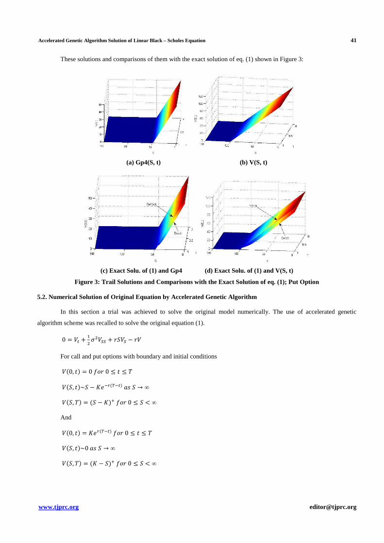
These solutions and comparisons of them with the exact solution of eq. (1) shown in Figure 3:

(a) Gp4(S, t) (b) V(S, t)

(c) Exact Solu. of (1) and Gp4 (d) Exact Solu. of (1) and V(S, t)

Figure 3: Trail Solutions and Comparisons with the Exact Solution of eq. (1); Put Option

5.2. Numerical Solution of Original Equation by Accelerated Genetic Algorithm

In this section a trial was achieved to solve the original model numerically. The use of accelerated genetic

algorithm scheme was recalled to solve the original equation (1).

0 = �� + �� + �� − �

For call and put options with boundary and initial conditions

��0, 4� = 0�m0 ≤ 4 ≤ 5

��, 4�~� − >DE@�TE��9I� → ∞

��, 5� = �� − >�H�m0 ≤ � < ∞

And

��0, 4� = >D@�TE��m0 ≤ 4 ≤ 5

��, 4�~09I� → ∞

��, 5� = �> − ��H�m0 ≤ � < ∞



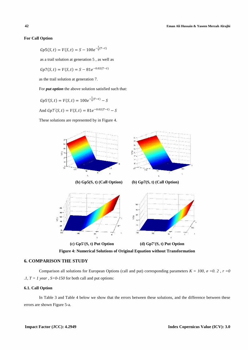
For Call Option

cd5��, 4� = ��, 4� = � − 100DEio�TE�� as a trail solution at generation 5 , as well as

cd7��, 4� = ��, 4� = � − 81DE�.��TE�� as the trail solution at generation 7.

For put option the above solution satisfied such that:

cd5′��, 4� = ��, 4� = 100DEio�TE�� − �

And cd7′��, 4� = ��, 4� = 81DE�.��TE�� − �

These solutions are represented by in Figure 4.

(b) Gp5(S, t) (Call Option) (b) Gp7(S, t) (Call Option)

(c) Gp5'(S, t) Put Option (d) Gp7'(S, t) Put Option

Figure 4: Numerical Solutions of Original Equation without Transformation

6. COMPARISON THE STUDY

Comparison all solutions for European Options (call and put) corresponding parameters K = 100, σ =0. 2 , r =0

.1, T = 1 year , S=0-150 for both call and put options:

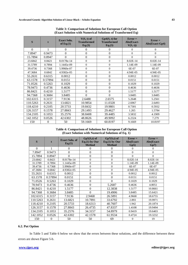
6.1. Call Option

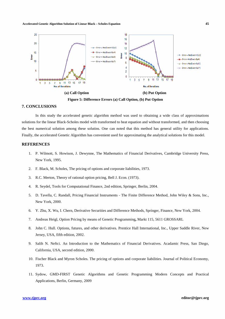
In Table 3 and Table 4 below we show that the errors between these solutions, and the difference between these

errors are shown Figure 5-a.



Table 3: Comparison of Solutions for European Call Option (Exact Solution with Numerical Solutions of Transformed Eq)

S t Exact Solu. of Eq.(1)

V(S, t) of Transformed

Eq.(3)

Gp4(S, t) for Transformed

Eq.(3)

Error = Abs(Exact-

V(S, t))

Error = Abs(Exact-Gp4)

0 1 0 0 0 0 0 7.8947 0.9473 0 0 0 0 0 15.7894 0.8947 0 0 0 0 0 23.6842 0.8421 8.0178e-14 0 0 8.02E-14 8.02E-14 31.5789 0.7894 1.1445e-09 0 0 1.14E-09 1.14E-09 39.4736 0.7368 5.9960e-07 0 0 6E-07 6E-07 47.3684 0.6842 4.9382e-05 0 0 4.94E-05 4.94E-05 55.2631 0.6315 0.0012 0 0 0.0012 0.0012 63.1578 0.57894 0.0151 0 0 0.0151 0.0151 71.0526 0.5263 0.1029 0 0 0.1029 0.1029 78.9473 0.4736 0.4636 0 0 0.4636 0.4636 86.8421 0.4210 1.5177 0 0 1.5177 1.5177 94.7368 0.3684 3.8485 0 0 3.8485 3.8485 102.6315 0.3157 7.9136 2.6488 2.6575 5.2648 5.2561 110.5263 0.2631 13.6821 10.9854 11.0328 2.6967 2.6493 118.4210 0.2105 20.5733 19.8432 19.9801 0.7301 0.5932 126.3157 0.1578 27.8843 29.1493 29.4627 1.265 1.5784 134.2105 0.1053 35.2576 38.8408 39.4485 3.5832 4.1909 142.1052 0.0526 42.6302 48.8626 49.9092 6.2324 7.279

150 0 50 59.1669 60.8197 9.1669 10.8197

Table 4: Comparison of Solutions for European Call Option (Exact Solution with Numerical Solutions of Eq. 1)


Gp5(S,t) of Eq.(1) by Our

Method

Gp7(S,t) of Eq.(1) by Our

Method

Error = Abs(Exact-

Gp5)

Error = Abs(Exact-

Gp7) 0 1 0 0 0 0 0

7.8947 0.9473 0 0 0 0 0 15.7894 0.8947 0 0 0 0 0 23.6842 0.8421 8.0178e-14 0 0 8.02E-14 8.02E-14 31.5789 0.7894 1.1445e-09 0 0 1.14E-09 1.14E-09 39.4736 0.7368 5.9960e-07 0 0 6E-07 6E-07 47.3684 0.6842 4.9382e-05 0 0 4.94E-05 4.94E-05 55.2631 0.6315 0.0012 0 0 0.0012 0.0012 63.1578 0.57894 0.0151 0 0 0.0151 0.0151 71.0526 0.5263 0.1029 0 0 0.1029 0.1029 78.9473 0.4736 0.4636 0 5.2687 0.4636 4.8051 86.8421 0.4210 1.5177 0 12.3838 1.5177 10.8661 94.7368 0.3684 3.8485 0 19.4906 3.8485 15.6421 102.6315 0.3157 7.9136 2.9468 26.5891 4.9668 18.6755 110.5263 0.2631 13.6821 10.7891 33.6792 2.893 19.9971 118.4210 0.2105 20.5733 18.6313 40.7607 1.942 20.1874 126.3157 0.1578 27.8843 26.4735 47.8337 1.4108 19.9494 134.2105 0.1053 35.2576 34.3157 54.8979 0.9419 19.6403 142.1052 0.0526 42.6302 42.1578 61.9534 0.4724 19.3232

150 0 50 50 69 0 19 6.2. Put Option

In Table 5 and Table 6 below we show that the errors between these solutions, and the difference between these

errors are shown Figure 5-b.



Table 5: Comparison of Solutions for European Put Option (Exact Solution with Numerical Solutions of Transformed Eq)


V(S, t) of Transformed

Eq.(3)

Gp4(S ,t) for Transformed

Eq.(3)

Error = Abs(Exact-

V(S, t))

Error= Abs(Exact-

Gp4) 0 1 90.4837 100.4385 98.0198 9.9548 7.5361

7.8947 0.9473 83.0664 92.5206 90.2283 9.4542 7.1619 15.7894 0.8947 75.6517 84.6027 82.4369 8.951 6.7852 23.6842 0.8421 68.2395 76.6849 74.6456 8.4454 6.4061 31.5789 0.7894 60.8299 68.7670 66.8545 7.9371 6.0246 39.4736 0.7368 53.4228 60.8492 59.0634 7.4264 5.6406 47.3684 0.6842 46.0183 52.9313 51.2724 6.913 5.2541 55.2631 0.6315 38.6176 45.0135 43.4816 6.3959 4.864 63.1578 0.5789 31.2321 37.0957 35.6908 5.8636 4.4587 71.0526 0.5263 23.9232 29.1779 27.9002 5.2547 3.977 78.9473 0.4736 16.8899 21.2600 20.1097 4.3701 3.2198 86.8421 0.4210 10.5525 13.3422 12.3193 2.7897 1.7668 94.7368 0.3684 5.4945 5.4244 4.5290 0.0701 0.9655 102.6315 0.3157 2.1735 0 0 2.1735 2.1735 110.5263 0.2631 0.5585 0 0 0.5585 0.5585 118.4210 0.2105 0.0689 0 0 0.0689 0.0689 126.3157 0.15789 0.0020 0 0 0.002 0.002 134.2105 0.1052 1.9454e-06 0 0 1.95E-06 1.95E-06 142.1052 0.0526 0 0 0 0 0

150 0 0 0 0 0 0

Table 6: Comparison of Solutions for European Put Option (Exact Solution with Numerical Solutions of Eq. (1))


Gp5'(S, t) of Eq.(1) by

Our Method

Gp7'(S, t) of Eq.(1) by Our

Method

Error = Abs(Exact-

Gp5')

Error = Abs(Exact-

Gp7')

0 1 90.4837 99.0049 79.396 8.5212 11.0877 7.8947 0.9473 83.0664 91.1623 71.5849 8.0959 11.4815 15.7894 0.8947 75.6517 83.3197 63.7739 7.668 11.8778 23.6842 0.8421 68.2395 75.4772 55.963 7.2377 12.2765 31.5789 0.7894 60.8299 67.6346 48.1521 6.8047 12.6778 39.4736 0.7368 53.4228 59.7921 40.3413 6.3693 13.0815 47.3684 0.6842 46.0183 51.9497 32.5307 5.9314 13.4876 55.2631 0.6315 38.6176 44.1072 24.7201 5.4896 13.8975 63.1578 0.5789 31.2321 36.2648 16.9096 5.0327 14.3225 71.0526 0.5263 23.9232 28.4224 9.0992 4.4992 14.824 78.9473 0.4736 16.8899 20.58 1.2888 3.6901 15.6011 86.8421 0.4210 10.5525 12.737 0 2.1845 10.5525 94.7368 0.3684 5.4945 4.8954 0 0.5991 5.4945 102.6315 0.3157 2.1735 0 0 2.1735 2.1735 110.5263 0.2631 0.5585 0 0 0.5585 0.5585 118.4210 0.2105 0.0689 0 0 0.0689 0.0689 126.3157 0.15789 0.0020 0 0 0.002 0.002 134.2105 0.1052 1.9454e-06 0 0 1.95E-06 1.95E-06 142.1052 0.0526 0 0 0 0 0

150 0 0 0 0 0 0



(a) Call Option (b) Put Option

Figure 5: Difference Errors (a) Call Option, (b) Put Option

7. CONCLUSIONS

In this study the accelerated genetic algorithm method was used to obtaining a wide class of approximations

solutions for the linear Black-Scholes model with transformed to heat equation and without transformed, and then choosing

the best numerical solution among these solutins. One can noted that this method has general utility for applications.

Finally, the accelerated Genetic Algorithm has convenient used for approximating the analytical solutions for this model.

REFERENCES

1. P. Wilmott, S. Howison, J. Dewynne, The Mathematics of Financial Derivatives, Cambridge University Press,

New York, 1995.

2. F. Black, M. Scholes, The pricing of options and corporate liabilities, 1973.

3. R.C. Merton, Theory of rational option pricing, Bell J. Econ. (1973).

4. R. Seydel, Tools for Computational Finance, 2nd edition, Springer, Berlin, 2004.

5. D. Tavella, C. Randall, Pricing Financial Instruments - The Finite Difference Method, John Wiley & Sons, Inc.,

New York, 2000.

6. Y. Zhu, X. Wu, I. Chern, Derivative Securities and Difference Methods, Springer, Finance, New York, 2004.

7. Andreas Heigl, Option Pricing by means of Genetic Programming, Markt 115, 5611 GROSSARL

8. John C. Hull. Options, futures, and other derivatives. Prentice Hall International, Inc., Upper Saddle River, New

Jersey, USA, fifth edition, 2002.

9. Salih N. Neftci. An Introduction to the Mathematics of Financial Derivatives. Acadamic Press, San Diego,

California, USA, second edition, 2000.

10. Fischer Black and Myron Scholes. The pricing of options and corporate liabilities. Journal of Political Economy,

1973.

11. Sydow, GMD-FIRST Genetic Algorithms and Genetic Programming Modern Concepts and Practical

Applications, Berlin, Germany, 2009



12. D.E. Goldberg, Genetic algorithms in search, Optimization and Machine Learning, Addison Wesley, 1989.

13. G. Tsoulos. I. E, Solving differential equations with genetic programming P.O. Box 1186, Ioannina 45110, 2003

14. P. Naur, “Revised report on the algorithmic language ALGOL, 1963.

15. E.A. Hussain and Y.M. Alrajhi , Solution of partial differential equations using accelerated genetic algorithm, Int.

J. of Mathematics and Statistics Studies, Vol. 2, No.1, pp. 55-69, March 2014.

16. M. O'Neill and C. Ryan, Under the hood of grammatical evolution, 1999.

17. M. O'Neill and C. Ryan, Grammatical Evolution: Evolutionary Automatic Programming in a Arbitrary Language,

Kluwer Academic Publishers, 2003.

18. M. O'Neill and C. Ryan, Grammatical Evolution, IEEE Trans. Evolutionary Computation, Vol. 5, pp. 349-358,

2001.

19. J. Ankudinova, The numerical solution of nonlinear Black–Scholes equations, Master’s Thesis, Technische

Universitat Berlin, 2008

20. Md. K. Salah Uddin, M. Ahmed, S. K. Bhowmik, A not on numerical solution of linear Black-Scholes model,

2013.

ACCELERATED GENETIC ALGORITHM SOLUTION OF LINEAR BLACK – SCHOLES EQUATION

Documents

Transcript of ACCELERATED GENETIC ALGORITHM SOLUTION OF LINEAR BLACK – SCHOLES EQUATION