University of Louisville University of Louisville

ThinkIR: The University of Louisville's Institutional Repository ThinkIR: The University of Louisville's Institutional Repository

Electronic Theses and Dissertations

5-2012

The Black-Scholes formula and volatility smile. The Black-Scholes formula and volatility smile.

Brian Michael Butler 1969- University of Louisville

Follow this and additional works at: https://ir.library.louisville.edu/etd

Recommended Citation Recommended Citation Butler, Brian Michael 1969-, "The Black-Scholes formula and volatility smile." (2012). Electronic Theses and Dissertations. Paper 188. https://doi.org/10.18297/etd/188

This Master's Thesis is brought to you for free and open access by ThinkIR: The University of Louisville's Institutional Repository. It has been accepted for inclusion in Electronic Theses and Dissertations by an authorized administrator of ThinkIR: The University of Louisville's Institutional Repository. This title appears here courtesy of the author, who has retained all other copyrights. For more information, please contact thinkir@louisville.edu.

THE BLACK-SCHOLES FORMULA AND VOLATILITY SMILE

By

Brian Michael Butler B.A., Humboldt State University, 1993

A Thesis Submitted to the Faculty of the

College of Arts and Sciences of the University of Louisville in Partial Fulfillment of the Requirements

for the Degree of

Master of Arts

Department of Mathematics University of Louisville

Louisville, Kentucky

May 2012

ii

THE BLACK-SCHOLES FORMULA AND VOLATILITY SMILE

By

Brian Michael Butler B.A, Humboldt State University, 1993

A Thesis Approved on

April 23, 2012

by the following Thesis Committee:

Ewa Kubicka, Thesis Director

Ryan Gill

DEDICATION

This thesis is dedicated to my wife

Kelly Estep

whose loving support and encouragement

guided me onward in my education,

and to our beautiful children, Aidan and Lily,

who we hope to provide with the educational

opportunities we received from our parents.

Also to my Great Aunt and Godmother, Hilda,

who in her usual gentle and loving way

encouraged me to persevere, and now it is done.

III

ACKNOWLEDGEMENTS

The author would like to extend thanks to Professor Ewa Kubicka for suggesting this

topic and providing the opportunity to explore it. Her knowledge and assistance were a

great aid in the preparation of this work.

IV

ABSTRACT

THE BLACK-SCHOLES FORMULA AND VOLATILITY SMILE

Brian M. Butler

April 23, 2012

This paper investigates the development and applications of the Black-Scholes

formula. This well-known formula is a continuous time model used primarily to price

European style options. However in recent decades, observations in financial market data

have brought into question some of the basic assumptions that the model relies on. Of

particular interest is the prevalence of the volatility smile in asset option prices. This is a

violation of one ofthe key assumptions under this model, and as a result alternatives to

and modifications of Black-Scholes have been suggested, some continuous and some

discrete. This paper researches one such modification, proposed by Derman and Kani

(1994), in which observed market data is used to create a discrete time implied asset price

tree that correctly reflects changing volatilities, risk-neutral probabilities, and observed

option prices. The results are then used to price a less conventional derivative

arrangement.

v

TABLE OF CONTENTS

PAGE

ABSTRACT ...................................................................................................................... v LIST OF TABLES ............................................................................................................ vi LIST OF FIGURES .......................................................................................................... vii

INTRODUCTION ............................................................................................................ 1

BACKGROUND .............................................................................................................. 4

Options ........................................................................................................................ 4

Risk ............................................................................................................................. 7

TRADING STRA TEGIES ................................................................................................ 9

Arbitrage ..................................................................................................................... 9

Market Efficiency ....................................................................................................... 10

Put-Call Parity ............................................................................................................. 11

THE PRICE PROCESS .................................................................................................... 14

The Memoryless Property and Stochastic Processes .................................................. 14

Random Walks and the Wiener Process ..................................................................... 15

The Black-Scholes Pricing Formula ........................................................................... 18

IMPLIED VOLA TIL TY IN DETAIL .............................................................................. 30

REFERENCES ................................................................................................................. 64

APPENDIX ....................................................................................................................... 66

CURRICULUM VITAE ................................................................................................... 68

VI

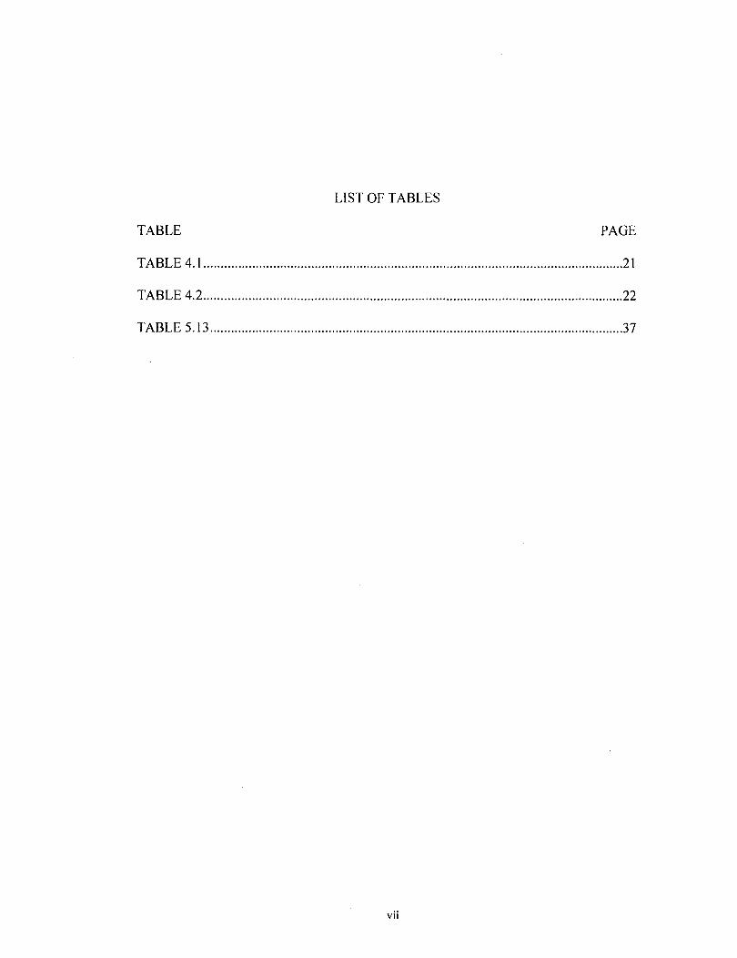
LIST OF TABLES

TABLE PAGE

TABLE 4.1 ......................................................................................................................... 21

TABLE 4.2 ......................................................................................................................... 22

TABLE 5.13 ....................................................................................................................... 37

vii

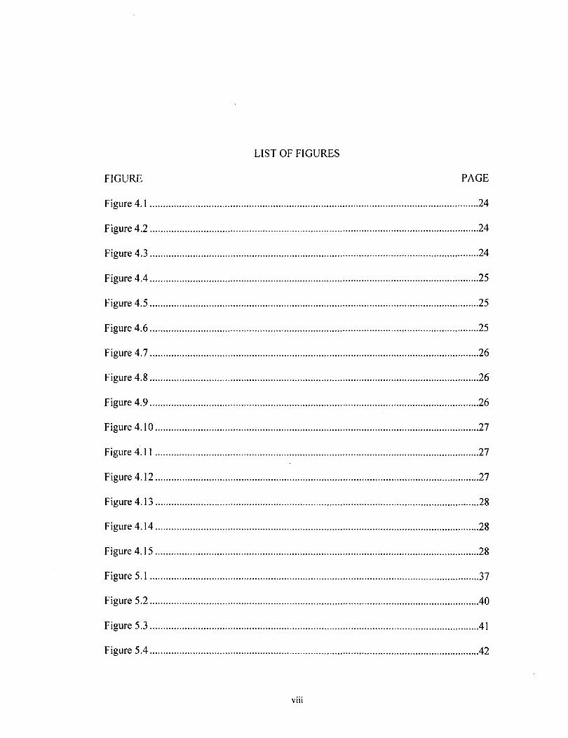
LIST OF FIGURES

FIGURE PAGE

Figure 4.1 ........................................................................................................................... 24

Figure 4.2 ........................................................................................................................... 24

Figure 4.3 ........................................................................................................................... 24

Figure 4.4 ........................................................................................................................... 25

Figure 4.5 ........................................................................................................................... 25

Figure 4.6 ........................................................................................................................... 25

Figure 4.7 ........................................................................................................................... 26

Figure 4.8 ........................................................................................................................... 26

Figure 4.9 ........................................................................................................................... 26

Figure 4.1 0 ......................................................................................................................... 27

Figure 4.11 ......................................................................................................................... 27

Figure 4.12 ......................................................................................................................... 27

Figure 4.13 ......................................................................................................................... 28

Figure 4.14 ......................................................................................................................... 28

Figure 4.15 ......................................................................................................................... 28

Figure 5.1 ........................................................................................................................... 37

Figure 5.2 ........................................................................................................................... 40

Figure 5.3 ........................................................................................................................... 41

Figure 5.4 ........................................................................................................................... 42

viii

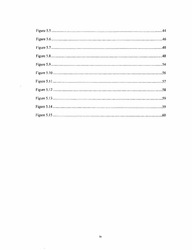
Figure 5.5 ........................................................................................................................... 44

Figure 5.6 ........................................................................................................................... 46

Figure 5.7 ........................................................................................................................... 48

Figure 5.8 ........................................................................................................................... 48

Figure 5.9 ........................................................................................................................... 54

Figure 5.1 0 ......................................................................................................................... 56

Figure 5.11 ......................................................................................................................... 57

Figure 5.12 ......................................................................................................................... 58

Figure 5.13 ......................................................................................................................... 59

Figure 5.14 ......................................................................................................................... 59

Figure 5.15 ......................................................................................................................... 60

ix

CHAPTER I

INTRODUCTION

Although stock markets as we know them have existed in recognizable form for

nearly five hundred years, it was not until surprisingly recently that some powerful

mathematical tools were applied in the field of finance (see Bru, et al [6]). In fact, not

until the middle of the twentieth century were probability models developed more fully

and used in financial applications. Since that time a large amount of mathematical

literature has been dedicated to financial applications, and in the last thirty years an entire

body of work has emerged that aims to address some of the practical, real world problems

encountered in pricing theory. In the early 1970s Black, Scholes, and Merton developed

explicit models for use in the pricing of options. Although the celebrated Black-Scholes

model has proven to be the foundation of modern financial engineering, it rests on a

series of assumptions about the market and those who engage in market activity. As a

result, the models can at times fail to capture some of the elements in the real-world

financial markets. Researchers have systematically modified various parts of the model to

address some of its shortfalls.

An area of particular interest is that of estimating volatility for the use in accurate

pricing and proper application of various pricing models. Essential to the Black-Scholes

formula and its variations are two parameter values - the drift rate and variance rate.

Simply put the drift rate is the average increase per unit time of a stochastic process, and

the variance rate is the average increase in the variance of the process per unit of time and

is also the square of the volatility. Volatility can be estimated from a history of the stock

price, where it is defined to be the standard deviation of the return provided by a stock

over a time period, when returns are expressed using continuous compounding. However

volatility can also be implied from observing option prices in the market.

Successfully incorporating the effects of risk into pricing theory not only yields a

more accurate representation of the market, but also allows for more sophisticated

financial engineering. Ultimately, the goal of financial engineering, as it pertains to risk,

is to develop strategies that minimize the variation in returns. In the absence of a money

machine, there should be no way to earn a riskless profit consistently from an efficiently

functioning capital market. However, the market consistently exposes traders and

investors to any of the types of risk just mentioned, and in the end the meaning of risk is

the same - it is the uncertainty of the outcome. Naturally mathematical models serve to

lend framework to the complex structure of the financial markets in an attempt to offer a

more complete understanding of the underlying dynamics. When this is achieved,

hedging strategies can be developed to counter the risk and make successful trading

possible in the presence of exposure. Although the risk is not alleviated entirely, ideally

speaking its impact can be minimized.

The purpose of this paper is to examine the mathematics of option pricing and the

options market, to summarize some of the research and findings regarding volatility

estimation, and to examine the effects of volatility on option pricing, and in particular the

occurrence of volatility skew. Real stock market data will be used to estimate the needed

values for option pricing, and a detailed example will be created to demonstrate the

2

changing effects ofvolatility on prices. The paper will begin with general background

information regarding options, risk, hedging, and pricing theory. More background will

be presented as it is required during the development of the model.

3

CHAPTER 2

BACKGROUND

2.1 Options

The word option has the same basic meaning when used in financial applications

as it does when used in everyday language. It simply refers to an action that is not

obligatory, but mayor may not be undertaken according to the discretion of the

participant. In finance this consists of the option to transfer an asset at some future date at

a set price. One party has the right to take action, while the other party is required to

adhere to the terms of the contract. The common types of options that will be discussed

are known as call and put options, each of these can be further classified as either

European or American.

Definition 2.1.1 A call option is a contract that gives the buyer the right to purchase a

specific quantity of an asset at a specified price (called the exercise price or strike price)

on or before a specified date (called the exercise date, expiration date, or maturity) as

called for by the contract. For stocks the standard quantity is 100 shares.

Definition 2.1.2 A put option is a contract that gives the writer the right to sell a specific

quantity of an asset at a specified price on or before a specified date as called for by the

terms of the contract.

Definition 2.1.3 An option that can be exercised only on the exercise date is known as a

European option.

4

Definition 2.1.4 An option that can be exercised at any time prior to the exercise date is

known as an American option.

As mentioned above, options are traded on organized exchanges, and it follows

that there should be some solid financial reasoning for buying and selling options. Every

option has a price, and in exchange for this price there is the chance of financial gain

from exercising the option. It is only natural that a formula for valuing options would be

developed that allows for consistent pricing and actually reflects elements of fairness

while capturing the impacts of risk. But before addressing risk and valuation models,

some elementary examples of options will be helpful. For completeness it is also

worthwhile to note the following conventions of options exchanges:

i) options are typically traded one hundred at a time,

ii) strike prices are in increments of $2.50 or $5.00, and

iii) the expiration date in the US is the third Friday of the expiration month.

In the options market, there are only two roles a trader can play - that of a purchaser of

an option (known as the holder) and that of a seller of an option (known as the writer).

These roles are also known as positions and a trader can have a different position for each

transaction and can even be in more than one position at a time.

Definition 2.1.5 An investor who has purchased an option is said to have taken the long

position.

Definition 2.1.6 An investor who has sold or written an option is said to have taken the

short position.

Example 2.1 Suppose that a stock is currently selling at $58, and a European call option

is purchased on 100 shares for $3.75 per share. The option has a maturity of six months

5

and a strike price of $60. If the stock is selling at $66 six months from now and the option

is exercised, then 100 shares can be purchased for $6000 and sold for $6600. Since the

cost of the option was $375, there is a gain of ($600 - $375) == $225 (in the absence of

taxes and transaction costs). If instead the stock is selling for $63 at maturity, it would

still be worthwhile to exercise the option (still ignoring taxes and transaction costs).

Although the difference ($6300 - $6000) == $300 is less than the cost of the option,

namely $375, and thus represents a loss of$75, it is wise to exercise the option in order to

partially offset the $375 cost of option. The option would not be exercised if the share

price in six months is below the exercise price, as this would only increase the loss.

Overall there are only three possibilities for the outcome of exercising an option from the

perspective of cash flow, namely a positive, zero, or negative cash flow can result. These

outcomes are known as in-the-money, at-the-money, and out-of-the-money options,

respectively.

The previous example gives some insight into the relationship between option

prices and the prices of underlying assets. Intuitively it seems that in the case of a

European call option, the potential for gain is dependent on how likely the stock price is

to increase. Specifically, the likelihood for the stock price to increase or decrease is

measured by volatility. What about the case ofa European put option?

Example 2.2 Suppose that a particular stock is currently selling at $40, and a European

put option is bought to sell 100 shares at a strike price of $45. The option has a maturity

of six months and a cost of$2.75 per share. If the stock is selling at $35 six months from

now and the option is exercised, then 100 shares can be purchased for $3500 and sold for

$4500. Ignoring taxes and transaction costs, this yields a gain of ($4500 - $3500) ==

6

$1000 less the option cost of$275, or $725 to the purchaser of the option.

Simply put, the purchaser of a call option looks to gain from stock price increases

and the purchaser of a put option looks to benefit from stock price decreases. Once again,

it can be seen that uncertainty in the market price of the stock lends itself to potential gain

in options trading. More specifically holders of options can benefit from increased

fluctuation if price changes work in their favor, but are not exposed to greater loss due to

that uncertainty if price changes do not work in their favor. In the latter case they simply

do not exercise the option. The remainder of this paper is primarily concerned with

models for the value of European call options and will concentrate on that from this

point.

Definition 2.2.1 A frictionless market is a theoretical market environment where no

additional costs from the trade (movement) of securities exist.

Definition 2.2.2 A competitive market is a theoretical market environment where traders

act as price takers without driving securities prices.

Theoretically financial markets would have no associated transaction costs, taxes,

or trade restrictions that impact pricing and unlimited trading would not affect pricing.

Although the frictionless market assumption has been the subject of many current

extensions of classical theory, a way to incorporate trade size into pricing theory has been

studied to a much lesser extent. It can be seen then that both Option Pricing with

Liquidity Risk and Liquidity Risk and Arbitrage Pricing Theory address the very real

situation in financial markets where the pricing process is affected by the supply and

demand of a security and the size and timing of its trade. So far, researchers have used

the concept of convenience yield to incorporate liquidity risk into pricing theory.

7

Convenience yield simply stated is the gain associated with holding an asset instead of

the derivative product. This indicates that there is a sense of risk associated with holding

on to a low demand item (lack of marketability in a timely manner). This idea has been

used in commodity market pricing, but for liquidity risk applications it fails to address a

basic issue. Although it is successful in incorporating the facet of liquidity risk that has to

do with inventory issues, and even exhibits conditions necessary to apply the usual

arbitrage pricing theory, it does not "explicitly capture the impact of different trade sizes

on the price. Consequently, there is no notion of bid/ask spread for the traded securities in

this model structure. This is a significant omission because all markets experience price

inelasticities (quantity impacts) and bid/ask spreads." [8]

8

3.1 Arbitrage

CHAPTER 3

TRADING STRATEGIES

Without a consistent method for the assessment and incorporation of risk factors

into derivative pricing, there exists the potential for traders to make a riskless profit. A

simple example of how this works is illustrated by considering the price of common

stock. If the situation existed where shares in the same company were trading in different

exchanges for different prices (perhaps due to inconsistent valuation methods or

exchange rate disparity), the efficient trader could buy low and sell high in "a single

stroke, thereby earning afree lunch. If the market did not drive prices of common stock

according to the mechanisms of supply and demand, thereby allowing the price to reach

equilibrium, this potential for a free lunch would continue.

Definition 3.1.1 The guarantee of a riskless profit resulting from a series oftrades in the

market is referred to as arbitrage.

Arbitrage typically results from disparities in price. The above example, though

oversimplified, illustrates the role that price disparity plays in giving rise to arbitrage

opportunity. Fortunately, mechanisms within capital markets work to ensure that

arbitrage opportunities, should they arise, diminish as security prices adjust to meet the

changing demand. Keep in mind that arbitrage refers to the guarantee of a riskless profit

is essential to understanding the development of option pricing models, trading strategies,

9

and hedging.

3.2 Market Efficiency

Definition 3.2.1 The Efficient Market Hypothesis states that all of the information

relevant to the price of a security is reflected in the current price.

The idea of efficient capital markets ultimately results from the observation that

security prices follow a random walk, which will be expanded on in Chapter 5. In general

there are three forms of market efficiency considered by economists - weak-form,

semistrong-form, and strong-form. The weak-form eliminates the use of historical

information as a means for an investor to earn returns above the market average. Such

information consists of past stock price changes and overall market activity, such as

trading volume. The capital markets in the U.S. are generally thought to follow weak­

form efficiency. The semi strong-form eliminates the use of any publicly available

information as a means for an investor to earn returns above the market average. When

this type of information is made available, a semi strong-form efficient market will

rapidly incorporate the information into the current security price. Clearly, a semistrong­

form efficient market implies that the market is also a weak-form efficient capital market.

There is a great deal of research indicating that capital markets function at his level, for

example see Fama, et al [13]. Finally is the level of efficiency that would eliminate the

use of all public and private information as a means for an investor to earn returns above

the market average. This strong-form efficiency of capital markets is not supported by

evidence. Any of the insider trading scandals of the last hundred years serves as an

example that private information can be used to earn excessive returns. However there is

no guarantee that those engaged in such activity can do so consistently without the risk of

10

legal repercussion.

3.3 Put-Call Parity

Allowing that the current stock prices incorporate all available public information

and that historical information itself cannot be used to earn excessive returns, excluding

insider trading, the ability for a trader to be guaranteed a riskless profit is the result of

price disparity. In the case of European options of the same class (meaning they have the

same strike price and maturity date), the prices of calls and puts are formulated in such a

way as to, in a sense, bind them to each other and the market itself. If this is not the case

then price disparity will arise and give way to arbitrage opportunity. The relationship

between the price of a European call option, a European put option, and the market is

known as the put-call parity.

Definition 3.3.1 The put-call parity is the relationship between two portfolios that

protects against arbitrage opportunities in the market. One portfolio consists of a

European call option with price c and cash holdings equal to Ke-rT, and the other consists

of a European put option with price p and one share of stock with current price So, such

that

c + K e -rt = p + So.

Here the term Ke-rT is the present value of the strike price, discounted by the risk­

free interest rate. The portfolio consisting of the purchased call option and the cash

necessary to accumulate to the strike price at time T must be equivalent to the purchased

put option and the current value of a share of the stock. In other words, put-call parity

states that these portfolios must have the same value now, or there will be a guaranteed

advantage to owning one over the other. Consider the following example.

11

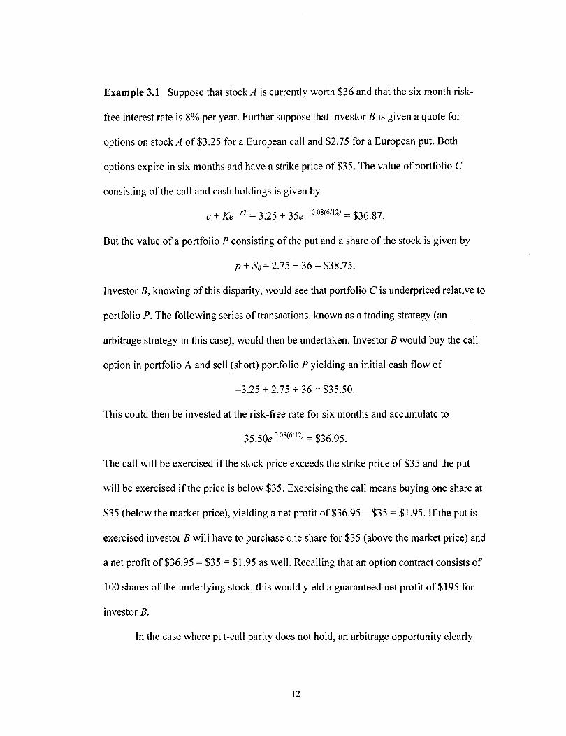
Example 3.1 Suppose that stock A is currently worth $36 and that the six month risk­

free interest rate is 8% per year. Further suppose that investor B is given a quote for

options on stock A of$3.25 for a European call and $2.75 for a European put. Both

options expire in six months and have a strike price of$35. The value of portfolio C

consisting of the call and cash holdings is given by

c + Ke-rT = 3.25 + 35e- 008(6/12) = $36.87.

But the value ofa portfolio P consisting of the put and a share of the stock is given by

p + So= 2.75 + 36 = $38.75.

Investor B, knowing of this disparity, would see that portfolio C is underpriced relative to

portfolio P. The following series of transactions, known as a trading strategy (an

arbitrage strategy in this case), would then be undertaken. Investor B would buy the call

option in portfolio A and sell (short) portfolio P yielding an initial cash flow of

-3.25 + 2.75 + 36 = $35.50.

This could then be invested at the risk-free rate for six months and accumulate to

35.50e 0.08(6/12) = $36.95.

The call will be exercised if the stock price exceeds the strike price of$35 and the put

will be exercised if the price is below $35. Exercising the call means buying one share at

$35 (below the market price), yielding a net profit of$36.95 - $35 = $1.95. If the put is

exercised investor B will have to purchase one share for $35 (above the market price) and

a net profit of $36.95 - $35 = $1.95 as well. Recalling that an option contract consists of

100 shares of the underlying stock, this would yield a guaranteed net profit of $195 for

investor B.

In the case where put-call parity does not hold, an arbitrage opportunity clearly

12

occurs. But in efficiently functioning capital markets, it exists only briefly until traders

exploit the disparity and supply and demand adjust the prices accordingly. This same

parity can be also used to derive the price of a call given the price of a put and the current

stock price, or to derive the price of a put given the call price and current stock price.

This type of simplified analysis can indicate the presence of arbitrage as in the preceding

example and similar examples can be used to illustrate the presence of arbitrage

opportunities under different circumstances, such as on options involving dividend­

paying stock. The end result is the same, namely that the unknowns that give rise to

arbitrage strategy are the prices of the options. If a model is used to price call and put

options in the absence of arbitrage opportunities, a variety of profit patterns arises

depending on the trading strategy. None of these profits is considered riskless, however,

and the problem arises of eliminating as much of the uncertainty as possible, a process

known as hedging.

13

CHAPTER 4

THE PRICE PROCESS

4.1 The Memoryless Property and Stochastic Processes

The widely accepted idea that capital markets function under weak-form

efficiency is crucial to the mathematics of option valuation. Recall that weak-form

efficiency indicates that above average returns cannot be earned by using historical

information, such as average returns, as a mechanism for predicting future price activity.

Mathematically speaking, this means that the underlying process that stock prices follow

must be a memoryless process. This leads to the following discussion of stochastic

processes, and eventually to the Black-Scholes Model.

Definition 4.1.1 A random variable X is said to be without memory, or memoryiess, if

Pr{X ~x + t I X> t} = Pr{X ~x} x, t> O.

The memoryless property is classically exhibited by the exponential distribution.

In words it means that the likelihood of a particular future outcome depends only on the

current state. The memory less property is also known as the Markov property, and is of

interest here as it relates to the memory less property of a stochastic process.

Definition 4.1.2 A stochastic process (or random process) is a family of random

variables {X(t), tE T}defined on a given probability space, indexed by the parameter t,

where t varies over an index set T.

F or completeness it should be noted that a random variable is itself a function

14

defined on a sample space S, so a stochastic process is actually a function of two

arguments. The convention of denoting a stochastic process as only X(t) will be adopted

here. Further, note that the set of all possible values for the random variables is referred

to as the state set or state space. Now in terms of a random process the memoryless

property can be redefined.

Definition 4.1.3 A stochastic process {X(t), t E T} is said to be Markov process if

Pr{X(tn + I) :s Xn + 1 I XUn) = Xn, X(tn -d = Xn-I , ... , X(tl) = xd = Pr{ X(tn + I) :s Xn + 1 I XUn) = Xn },

whenever tl < t2 < ... < tn < tn + I. A discrete-state Markov process is called a Markov

chain.

The relationship illustrated by the above definition is known as the Markov

property, or memory less property. It indicates that the future state of such a process is not

determined by the past states or past history of the process, but only by the current state.

More specifically, the Markov property shows no dependence on the manner in which the

current state arose, but only on the current state itself. The thought here is that all of the

previous information, prior to the current state of the process, is inherently integrated into

the current state, and only this current state is a factor. In terms of stock prices and weak­

form efficiency, it is clear that the underlying price process of stocks could be described

by a Markov process.

4.2 Random Walks and the Wiener Process

Early investigation into stock prices, such as that conducted by Kendall [18], was

done in part to expose cyclical patterns in the markets. Such research only reinforced

even earlier work, such as that done by Bachelier, suggesting that stock price movements

were actually random processes. In fact, Bachelier's work had largely slipped out of

15

view, although his development of the mathematics of random processes predated even

Einstein, whose work on colliding gas molecules relied heavily on a particular type of

random process known as Brownian mOlion. Brownian motion is used generically to

describe the motion of a collection of particles that are subject to a random walk. A

random walk in turn is typically described as a discrete Markov process composed of a

number of independent steps. Whereas the Markov property ensures that only the current

state is relevant to future stock prices, an extended period of observation time in the

future has some effect on the amount of uncertainty in the value in the future. So these

rates are proportional to the length of the interval (or index set) T.

Definition 4.2.1 The drift rate is defined to be the average increase per unit time of a

stochastic process.

Definition 4.2.2 The variance rate is defined to be the average increase in the variance of

the process per unit of time.

Definition 4.2.3 A variable Z is said to follow a particular type of Markov process,

known as a Wiener process if the following properties are satisfied:

Property 1. The change b.z during a small period of time I is b.z::=: £Jt;i , where £

is a random drawing from the standard normal distribution A{O, 1).

Property 2. The values for b.z l and b.z2 that correspond to any two non­

overlapping short intervals of time, tltl and /'0,,-'2, are independent.

It follows immediately then that b.z follows a normal distribution with mean 0 and

variance tll since

E[tlz] ::=: E[ £Jt;i] ::=: (Jt;i) E[ £] ::=: 0, and

Yar[tlz] ::=: Yar[ £Jt;i] ::=: (..[i;i )2Yar[ £] ::=: tll.

16

I f the limit as !::.t - 0 is considered, then a generalized Wiener process for a variable X

can be defined in terms of a Wiener process dZ, as dX = a dt + b dZ, where a and bare

constants representing incremental drift and variance rates respectively. Again

considering the discrete version over a small time interval !::.t, this becomes

!::.x = a !::.t + b &.[i;i .

It then follows that

E[!::.X] = E[a !::.t + b &.[i;i] = E[a !::.t] + E[b &.[i;i] = a !::.t + bE[!::.z] = a!::.t,

Yar[!::.X] = Yar[a!::.t + b &.[i;i] = 0 + b2Yar[!::.z] = b2!::.t.

If a longer interval of time is considered, say from 0 to T, it turns out that the mean

increase in x over the interval (drift rate) is aT and the variance of change over the

interval (variance rate) is b2T. This suggests that although a generalized Wiener process

may seem an ideal model for stock price changes, it fails in one important respect.

Recalling that the expected return and the stock price are independent, it is wrong to

assume a constant drift rate over an interval. An appropriate adjustment gives way to a

working model that uses geometric Brownian motion instead, where the expected return

(drift divided by price) is constant. The discrete-time version of geometric Brownian

motion for the change !::.S in stock price S, in a short interval of time !::.t is

!::.S = j.JS!::.t + as &.[i;i .

The Black-Scholes differential equation is derived from this relationship, and is not

dependent on the expected return. Solutions to the Black-Scholes differential equation

yield the equations used to price various options, including the European call options

with which this paper is concerned. Since expected returns have been removed from the

option pricing formula, all investors expect to obtain the same price for a particular

17

option. As will be shown in the next section, the Black-Sholes model makes a number of

assumptions that allow for this fair valuation to happen.

4.3 The Black-Scholes Pricing Formula

A method such as the Binomial Model (see Hull [14] or Shreve [28]) to price

stock options introduces some properties that are desirable to retain in a model such as

the Black-Scholes model. Namely, a riskless portfolio can be created and, in the absence

of arbitrage, the return is the risk-free interest rate.

Definition 4.3.1 A portfolio is said to be a riskless portfolio if it consists of holdings of a

stock and options on that stock such that there is no uncertainty about the portfolio value

at expiration.

In a Black-Scholes economy, a position in the option and stock portfolio is riskless for

only a very brief time. The following example illustrates an important result of this.

Example 4.1 Suppose that the price movements of a particular stock, S, and a European

call option, c, change according to the equation ~c = 0.3M, at some particular time. At

that time, a riskless portfolio would consist of purchasing 0.3 shares of the stock and

sell ing one call option.

But as time goes on the relationship between ~c and M will vary. As a result, the

portfolio must be rebalanced as frequently as the relationship changes. This is essential to

the Black-Scholes pricing formulas, and introduces the problem of liquidity risk. Since

rebalancing consists of making transactions, and transactions not only incur costs

directly, but can also impact prices (according to supply and demand effects) thereby

creating costs indirectly, the frequency of rebalancing has an obvious cost. Very frequent

rebalancing would certainly get expensive quickly. And the continuous rebalancing

18

necessary for the perfect hedge in the Black-Scholes model is impossibly expensive in

the face of transaction costs. As for the derivation of the Black-Scholes Model itself,

several assumptions were made:

1. The stock price follows the process !'!..S = JiSM + (J'S/),z , with Ii and (J'constant.

2. Short selling with full use of proceeds is allowed.

3. There are no transaction costs or taxes (frictionless).

4. The stock pays no dividend during the option life.

5. There are no riskless arbitrage opportunities.

6. Trading is continuous.

7. The risk-free rate, r, is constant and is the same for options of all maturities.

Under these assumptions, the Black-Scholes differential equation [4] was derived, a

solution to which yields the following equation.

Equation 4.3.1 The Black-Scholes formula for the price of a European call option at

time zero, on a non-dividend-paying stock is given by

c = SolVed]) - Xe-rTN(d2), where

d] = [In(SolX) + (r + (j 2/2)1] 1 [(J'/f]

and

N(x) is the cumulative probability distribution function of the standard normal variable,

So is the stock price at time 0, X is the strike price, (j is the volatility, and T is the time to

maturity of the option. There are some boundary conditions inherent in the model which

are discussed in some detail in Hull [14], but will not be discussed here. Additional

definitions will add to the overall understanding of the model and lead nicely into the

topic of volatility.

19

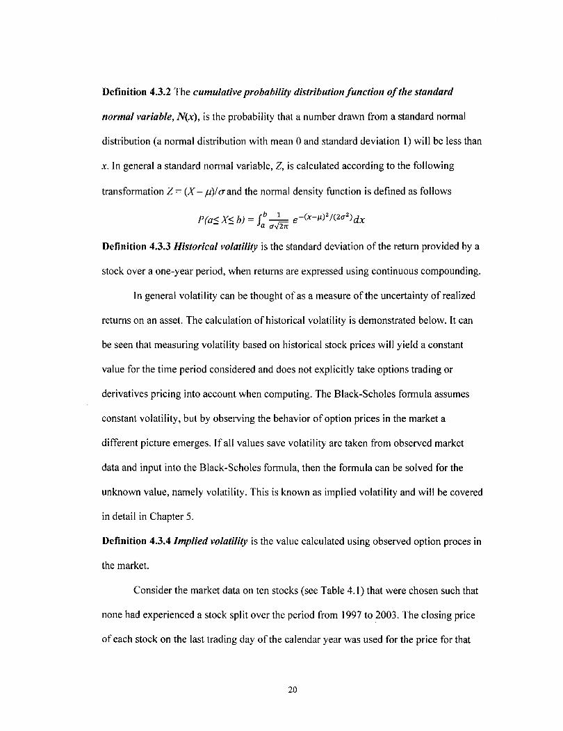
Definition 4.3.2 The cumulative probability distribution function of the standard

normal variable, N(x), is the probability that a number drawn from a standard normal

distribution (a normal distribution with mean 0 and standard deviation 1) will be less than

x. In general a standard normal variable, Z, is calculated according to the following

transformation Z = (X - fL)/ (]" and the normal density function is defined as follows

P/a<X<b\ = rb_l_ e-(x-/l)2/(2a2)dx I' - - 'j Ja a..['iIT

Definition 4.3.3 Historical volatility is the standard deviation of the return provided by a

stock over a one-year period, when returns are expressed using continuous compounding.

In general volatility can be thought of as a measure of the uncertainty of realized

returns on an asset. The calculation of historical volatility is demonstrated below. It can

be seen that measuring volatility based on historical stock prices will yield a constant

value for the time period considered and does not explicitly take options trading or

derivatives pricing into account when computing. The Black-Scholes formula assumes

constant volatility, but by observing the behavior of option prices in the market a

different picture emerges. If all values save volatility are taken from observed market

data and input into the Black-Scholes formula, then the formula can be solved for the

unknown value, namely volatility. This is known as implied volatility and will be covered

in detail in Chapter 5.

Definition 4.3.4 Implied volatility is the value calculated using observed option proces in

the market.

Consider the market data on ten stocks (see Table 4.1) that were chosen such that

none had experienced a stock split over the period from 1997 to 2003. The closing price

of each stock on the last trading day of the calendar year was used for the price for that

20

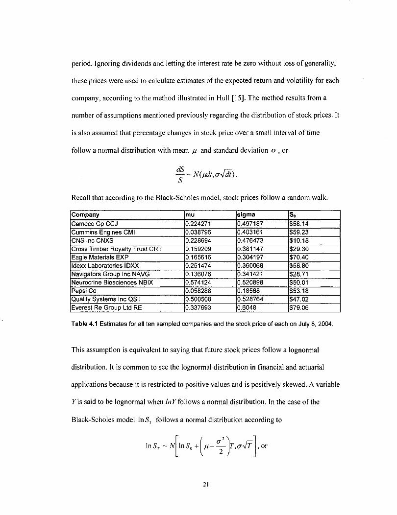
period. Ignoring dividends and letting the interest rate be zero without loss of generality,

these prices were used to calculate estimates of the expected return and volatility for each

company, according to the method illustrated in Hull [JS]. The method results from a

number of assumptions mentioned previously regarding the distribution of stock prices. It

is also assumed that percentage changes in stock price over a small interval of time

foIlow a normal distribution with mean j.1 and standard deviation a, or

dS r,: - ~ N(j.idt,a....;dt). S

Recall that according to the Black-Scholes model, stock prices follow a random walk.

Company mu sigma So Cameco Cp CCJ 0.224271 0.497187 $58.14 Cummins Engines CMI 0.038796 0.403161 $59.23 CNS Inc CNXS 0.228694 0.476473 $10.18 Cross Timber Royalty Trust CRT 0.159209 0.381147 $29.30 Eagle Materials EXP 0.165616 0.304197 $70.40 Idexx Laboratories IDXX 0.251474 0.360068 $58.80 Navigators Group Inc NAVG 0.136076 0.341421 $28.71 Neurocrine Biosciences NBIX 0.574124 0.520898 $50.01 Pepsi Co 0.058288 0.18568 $53.18 Quality Systems Inc QSII 0.500508 0.528764 $47.02 Everest Re Group Ltd RE 0.337693 0.6048 $79.06

Table 4.1 Estimates for all ten sampled companies and the stock price of each on July 8, 2004.

This assumption is equivalent to saying that future stock prices follow a lognormal

distribution. It is common to see the lognormal distribution in financial and actuarial

applications because it is restricted to positive values and is positively skewed. A variable

Yis said to be lognormal when InY follows a normal distribution. In the case of the

Black-Scholes model InSr follows a normal distribution according to

21

Sr [( (J"2) r;;;] Ins:--N 11- 2 T,(J"-yT ,

where N(m,n) is the cumulative normal distribution with mean m and standard deviation

n, and Sr is the stock price at a future time T. When T = 1, In Sr is the continuously So

compounded return over one year.

Definition 4.3.4 The ratio of an asset price in a given period of time to its price in the

preceding period is known as the price relative.

Since the interval of observation used here is one year, an estimate for the

expected return on a stock can be found by averaging the price relatives over the period

of observation. The volatility can then be estimated as the standard deviation of the

natural log of the price relatives over the period of observation. Table 4.2 shows the

specific calculation for one of the ten sampled companies, CCJ.

Cameco Cp CCJ Year i Close mu sigma 2003 19 $57.60 1.40501 0.877554 2002 18 $23.95 -0.03271 -0.03326 2001 17 $24.76 0.414857 0.347029 2000 16 $17.50 0.157025 0.145852 1999 15 $15.13 -0.15088 -0.16355 1998 14 $17.81 -0.44767 -0.59362 1997 13 $32.25

expected return 0.224271 vo/atilty estimate 0.497187

Table 4.2 Estimates for the expected return and volatility of CCJ stock.

We now have a model for pricing a European caIl option that captures the essence

of stock price movements as a memory less random process. This process consists of a

number of independent movements, each increment of which is drawn from a normal

distribution. Furthermore, all of the parameters necessary for applying Equation 4.3.1 can

be obtained from available data. An important element to first explore is the relationship

22

between these parameters and the option price generated by the Black-Scholes formula.

Although the relationship between volatility and option price is the most useful in the

present work, the effects of time-to-maturity, strike price, and current asset price on

option price will also be investigated.

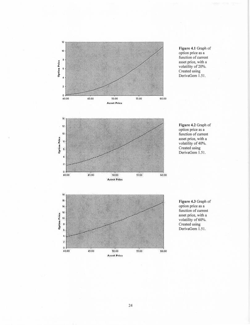
In the following figures, graphic representations of these relationships are

presented. Each graph was generated using DerivaGem 1.51 and in each case a risk free

interest rate of 3% was used. Figure 4.1, Figure 4.2, and Figure 4.3 illustrate the effect

that current asset price (So) has on the option price for securities with a volatility of20%,

40%, and 60% respectively. (In general so-called old economy securities have a volatility

in the range between 20% and 40%, whereas new economy securities have a volatility

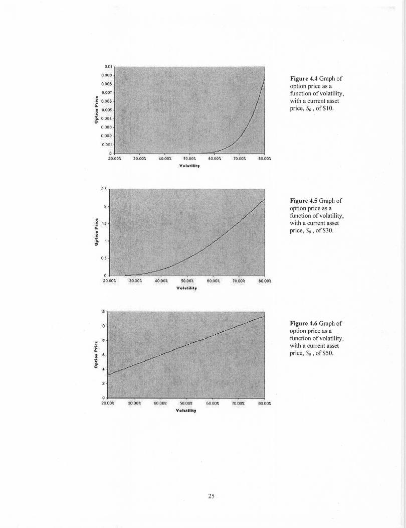
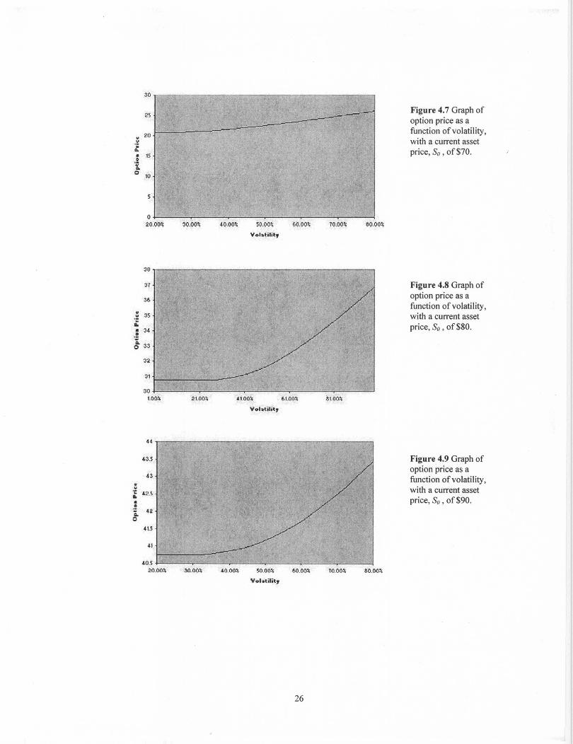
between 40% and 60%, Hull [14]). The effect that volatility has on option price for

securities with various prices is represented in Figure 4.4 - 4.9. And finally the effect that

strike price has on option price for a number of securities with various current prices and

volatilities is represented in Figure 4.10 - 4.15. The relationship between option price and

time-to-maturity is not as certain however.

These graphs are only representative of the general trend occurring when certain

variables are allowed to change. More specifically, the value ofa European call option

increases as the price of the underlying stock increases, ceter paribus (all other values

unchanged). In Figures 4.4 -- 4.9 it can be seen that as the volatility on a given security

increases the option value also increases, ceter paribus. So the greater the likelihood of

large price changes, the greater the potential payoff and, therefore, the more valuable the

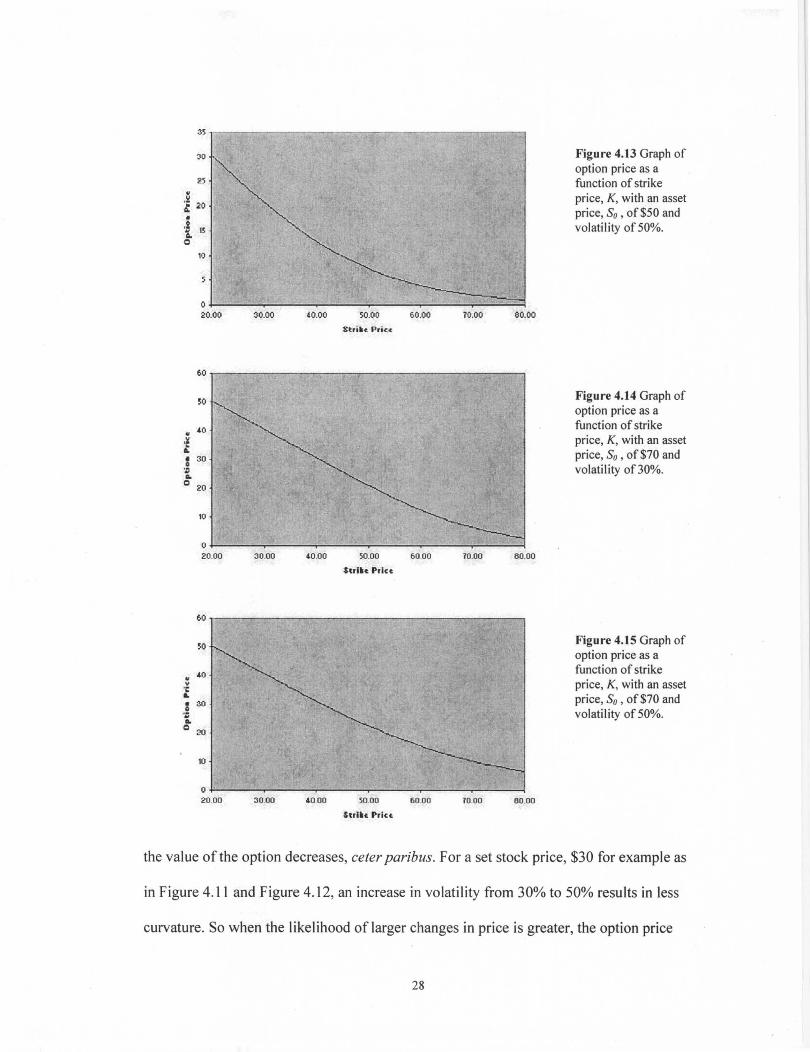
option. In Figures 4.10 - 4.15 it can be seen that as the strike price on an option increases

23

.. .!! ~ • . 2 '&. 0

10

2

o~~~--~----~--~------~--------~ 40.00 45.00 50.00 55.00 60.00

Asset Price

141---------------~~------------~~--~~----_,

12

10

, 2

O~----------~--------~~--------~------~--~ 40.00 45.00 50.00 55.00 £>0.00

.... "nt Prlc~

18

16

14

12

10

&

&

2

0 40.00 45.00 50.00 55.00 60.00

As~et Price

24

Figure 4.1 Graph of option price as a function of current asset price, with a volatility of 20%. Created using DerivaGem 1.51.

Figure 4.2 Graph of option price as a function of current asset price, with a volatility of 40%. Created using DerivaGem 1.51.

Figure 4.3 Graph of option price as a function of current asset price, with a volatility of 60% . Created using DerivaGem 1.51.

0.01

o.oos Figure 4.4 Graph of

0.008 option price as a O.OOT function of volatility, ..

.lI! 0.00& with a current asset ~ price, So , of $10. • 0.005 .2 '&. 0.004 C

0.003

0.002

0.001

0 20.00;: 30.00~ 40 .00~ 50.00~ 60.00~ TO.OO~ 80.00~

Yol.lilit,

2.5

Figure 4.5 Graph of 2 option price as a

" function of volatility,

.~ 1.5 with a current asset ~ price, So, of$30. • .2 '&. c

O.S

0 20.00l; 30.00l; 40.00l; 50.00l; ~O.OOl; TO.OOl; 80.00);

Yol.lili"

12

10 Figure 4.6 Graph of option price as a

.. 8 function of volatility,

... with a current asset ~ price, So, of$50. • 6 0 .:; .. I:) ,

2

0 20.00),: 30.00" 40.00" 50.001: &0.00" 10.00" 80.00),;

Yol.Ulit,

25

30

25 Figure 4.7 Graph of option price as a

20 function of volatility, .. with a current asset \I

~ price, So, of$70. • 15 0 Ii 0

10

O~----~-------r------~----~-------r----~ 20.00~ 40.00~ 50.00~ &O.OO~ 70.00% 80.00%

Volatilit,

36

3 7 Figure 4.8 Graph of

36 option price as a function of volatility, ..

35 with a current asset .l: 8: price, So, of$80. • 3' . !

8- 33

32

31

30 1.00% 21.00% 41.00% 61.00% 3 1.00%

Vol .. lilil,

44

43.5 Figure 4.9 Graph of

'3 option price as a

.. function of volatility, u with a current asset '1: '2.5 .. price, So, of$90 . • . !

42 i. 0

41.5

41

,o.5 20.00% 30.00% 40.00% 50.00% 60.00% TO.OO% 80.00%

Yol .. tilit,

26

12

10 Figure 4.10 Graph of option price as a

6 function of strike " .l! price, K, with an asset

A: price, So , of $30 and • 6 . ~ volatility of30%. 1 0

4

2

30.00 40.00 50.00 60.00 TO.OO M.OO

Shiklt: Pric~

12

10 Figure 4.11 Graph of option price as a

8 function of strike ~

Ie price, K, with an asset A.

price, So, of$30 and • 6 ,~ volatility of50% . ... CI

4

2

0 20.00 30.0 0 40.00 50.00 60 .00 10.00 60.00

$uih Price

35

30 Figure 4.12 Graph of option price as a

25 function of strike ., price, K, with an asset y

:f 20

S price, So, of$50 and 'D 15 volatility of30%. ... CI

10

O~----~------~----~--~~~~~ .. ----~ 20. 00 30.00 40.00 50.00 60.00 10.00 60.00

27

30

25

~ ~ 20

• o Ii 15 Q

10

0 20.00

60

50

~ 40

,~

.t • 30

.~ ... Q

20

10

0 20.00

60

50

~ 40

y

·c &.

• 30 0 . ~ ...

Q 20

10

0 20.00

30.00

30.00

30.00

40.00

40.00

40.00

50.00

S:tri.~ P,i<t:<f:

50.00

'ulh Prlc~

50.00

'trih Prlu

&0.00

60.00

60.00

10.00 eo.oo

10.00 60.00

10.00 60.00

Figure 4.13 Graph of option price as a function of strike price, K, with an asset price, So , of $50 and volatility of50%.

Figure 4.14 Graph of option price as a function of strike price, K, with an asset price, So , of $70 and volatility of30% .

Figure 4.15 Graph of option price as a function of strike price, K, with an asset price, So, of$70 and volatility of 50% .

the value of the option decreases, ceter paribus. For a set stock price, $30 for example as

in Figure 4.11 and Figure 4.12, an increase in volatility from 30% to 50% results in less

curvature. So when the likelihood of larger changes in price is greater, the option price

28

seems to decrease more gradually.

The general effects are of interest here and are as follows: an increase in stock

price causes an increase in option price, an increase in volatility causes an increase in

option price, and an increase in strike price causes a decrease in option price. In the

current work it is assumed without loss of generality that the risk-free interest rate is zero,

that the stocks are all non-dividend paying, and that all call options have a six-month

maturity. For completeness it should be noted then that as the risk-free rate increases the

value of the option increases. However as the time to expiration increases, the general

effect is uncertain. Dividends present a slightly more complicated situation in that

dividend payment lowers the stock price at the time the trade takes place, known as the

ex-dividend date. Also the value of the option is affected based on the anticipated

dividend, and in the case of a call option, its value is negatively affected by an expected

dividend.

29

CHAPTERS

IMPLIED VOLA TIL TY IN DETAIL

As discussed in Chapter 4, the historical volatility that can be calculated from

observed stock prices is constant for the period considered. As a practical application,

one would observe a six month history in order to calculate the historical volatility for

use in pricing a six-month option on the same underlying asset. However by observing

the prices of six-month options on a stock for different strike prices on a given day, the

implied volatility can be calculated using an option pricing model such as the Black­

Scholes formula. Recall that there are a number of assumptions at the heart of the Black­

Scholes formula, some of which are not a strict requirement under the framework. In fact

some assumptions have been relaxed in many cases, or an alternative approach has been

found that allows the assumption to be modified. A good example is the assumption that

the stock pays no dividend during the option life. As previously mentioned this is known

as an ex-dividend date, and alternative models exist for using the Black-Scholes

framework to price options when there is a dividend payment during the life of the

option. However a more crucial assumption lies at the base of the Black-Scholes

framework that has sparked a lot of curiosity and research, namely the assumption that

the volatility of the underlying equity is constant.

The primary assumption of the Black-Scholes formula is that stock prices follow

the process I~.s = jJSM + aSi1z , with p and a constant. Dividing both sides by the stock

30

price S leads back to the previous discussion regarding the lognormality of stock prices.

Note that the assumption made is not simply that the volatility on a given equity is

constant, but that it is constant across different strike prices. Therefore by collecting

market data on call options for a given stock for a variety of strike prices, with the same

time to maturity, the implied volatility for the underlying stock can be calculated using

the Black-Scholes formula (Formula 4.3.1 above). If the underlying assumption of Black­

Scholes framework holds then the obvious, expected result would be that the implied

volatility is constant for that stock.

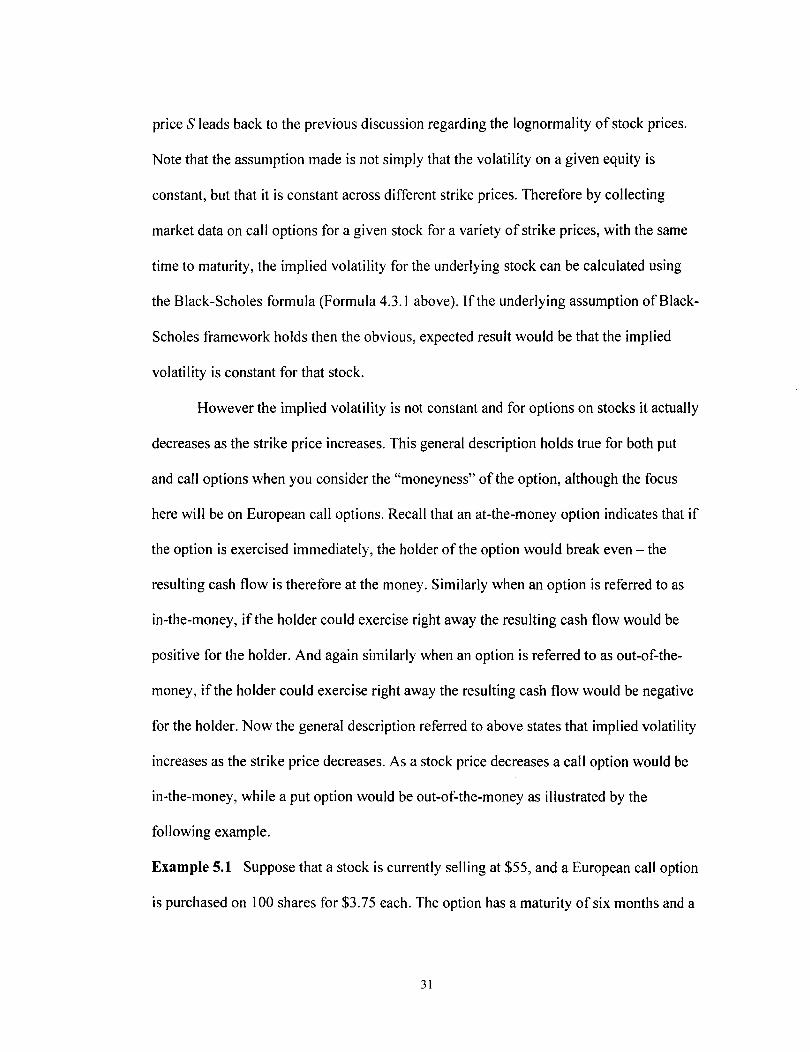
However the implied volatility is not constant and for options on stocks it actually

decreases as the strike price increases. This general description holds true for both put

and call options when you consider the "moneyness" of the option, although the focus

here will be on European call options. Recall that an at-the-money option indicates that if

the option is exercised immediately, the holder of the option would break even - the

resulting cash flow is therefore at the money. Similarly when an option is referred to as

in-the-money, if the holder could exercise right away the resulting cash flow would be

positive for the holder. And again similarly when an option is referred to as out-of-the­

money, if the holder could exercise right away the resulting cash flow would be negative

for the holder. Now the general description referred to above states that implied volatility

increases as the strike price decreases. As a stock price decreases a call option would be

in-the-money, while a put option would be out-of-the-money as illustrated by the

following example.

Example 5.1 Suppose that a stock is currently selling at $55, and a European call option

is purchased on 100 shares for $3.75 each. The option has a maturity of six months and a

31

strike price of $50. If the holder of the option could exercise it at that moment, the

resulting cash flow would be as follows. The holder would receive 100 shares for $5,000

after initially spending $375 on the options, for a total expenditure of$5,375. However,

the 100 newly acquired shares of stock are worth $55 per share on the market for a total

of$5,500 resulting in a positive cash flow of$125 (in the absence of taxes and

transaction costs). Suppose instead that the 100 options under consideration were for a

European put selling for $1.90 each. Then holder would have to sell 100 shares for $50

each when they are worth $55 each on the open market. This would result in a negative

cash flow of $190 for the options themselves and a market loss of $500 for a negative

cash flow of $690 for the holder of the put.

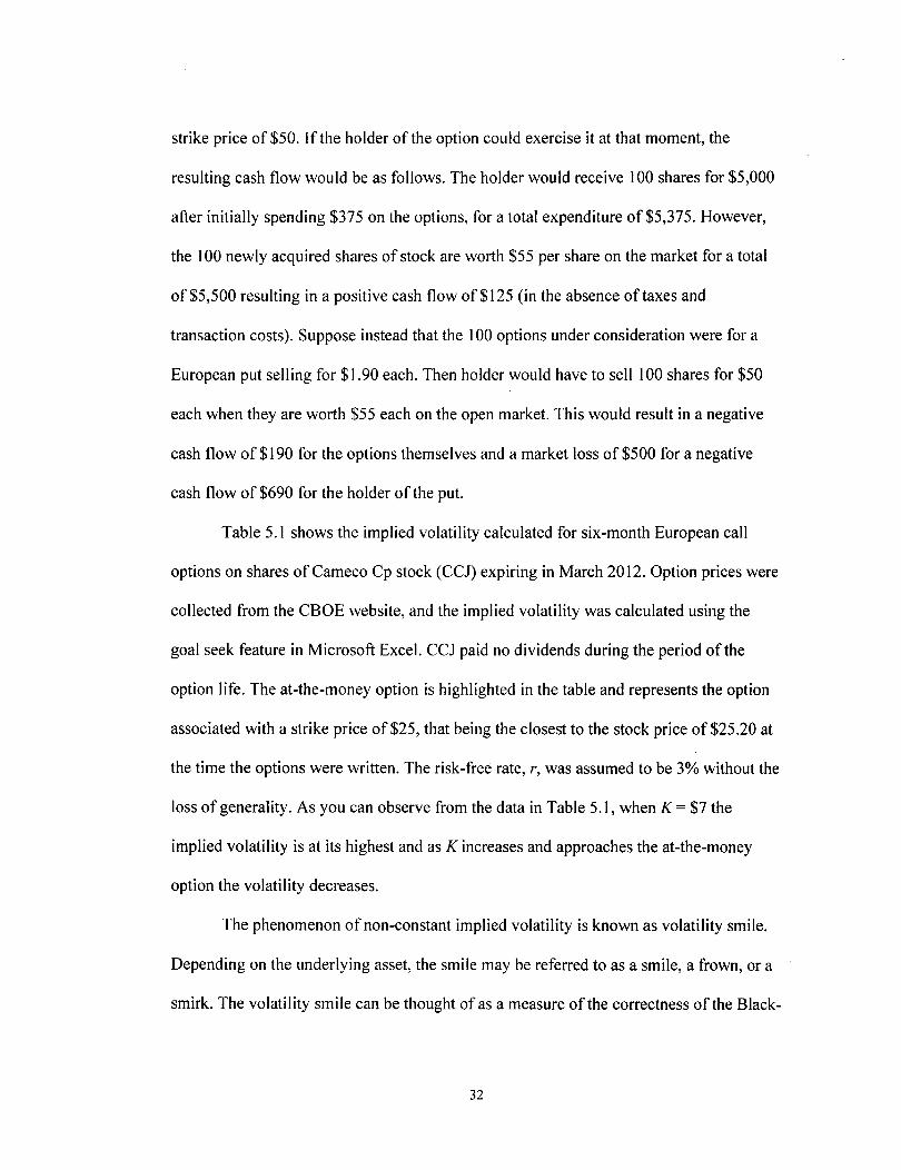
Table 5.1 shows the implied volatility calculated for six-month European call

options on shares of Came co Cp stock (CCl) expiring in March 2012. Option prices were

collected from the CBOE website, and the implied volatility was calculated using the

goal seek feature in Microsoft Excel. CCl paid no dividends during the period of the

option life. The at-the-money option is highlighted in the table and represents the option

associated with a strike price of $25, that being the closest to the stock price of $25.20 at

the time the options were written. The risk-free rate, r, was assumed to be 3% without the

loss of generality. As you can observe from the data in Table 5.1, when K = $7 the

implied volatility is at its highest and as K increases and approaches the at-the-money

option the volatility decreases.

The phenomenon of non-constant implied volatility is known as volatility smile.

Depending on the underlying asset, the smile may be referred to as a smile, a frown, or a

smirk. The volatility smile can be thought of as a measure of the correctness of the Black-

32

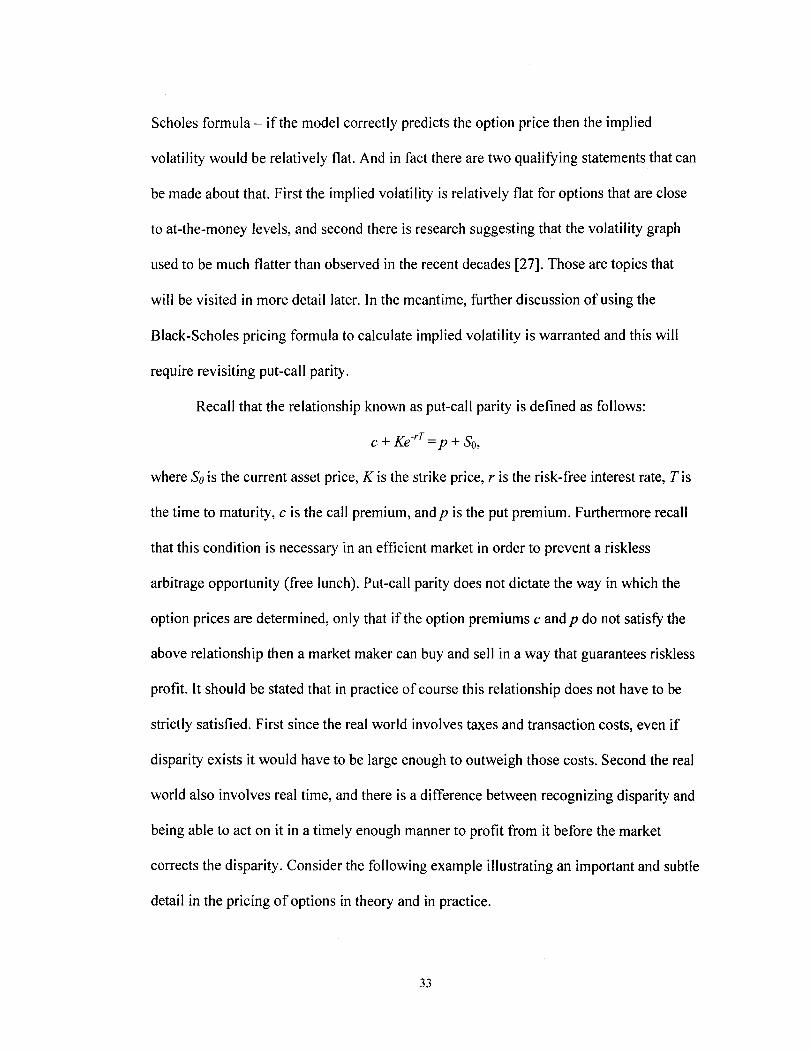
Scholes formula - if the model correctly predicts the option price then the implied

volatility would be relatively flat. And in fact there are two qualifying statements that can

be made about that. First the implied volatility is relatively flat for options that are close

to at-the-money levels, and second there is research suggesting that the volatility graph

used to be much flatter than observed in the recent decades [27]. Those are topics that

will be visited in more detail later. In the meantime, further discussion of using the

Black-Scholes pricing formula to calculate implied volatility is warranted and this will

require revisiting put-call parity.

Recall that the relationship known as put-call parity is defined as follows:

v -rT (' C + .o..e = p + DO,

where So is the current asset price, K is the strike price, r is the risk-free interest rate, Tis

the time to maturity, c is the call premium, and p is the put premium. Furthermore recall

that this condition is necessary in an efficient market in order to prevent a riskless

arbitrage opportunity (free lunch). Put-call parity does not dictate the way in which the

option prices are determined, only that if the option premiums c and p do not satisfy the

above relationship then a market maker can buy and sell in a way that guarantees riskless

profit. It should be stated that in practice of course this relationship does not have to be

strictly satisfied. First since the real world involves taxes and transaction costs, even if

disparity exists it would have to be large enough to outweigh those costs. Second the real

world also involves real time, and there is a difference between recognizing disparity and

being able to act on it in a timely enough manner to profit from it before the market

corrects the disparity. Consider the following example illustrating an important and subtle

detail in the pricing of options in theory and in practice.

33

Example 5.2 Let Krepresent the call option premium set by the market and Jrrepresent

the put premium as set by the market. Then let c and p represent the call and put option

premiums respectively as calculated using the Black-Scholes formula. Then by put-call

parity we have the following for the market price:

v -rT S S v -rT K+ I\.e = Jr+ 0, or K - Jr= 0- I\.e .

And we have the following for the Black-Scholes prices

v -rT S S v -rT C + I\.e = p + 0 or c - p = 0 - I\.e .

Since mathematically two expressions that are equal to a third are themselves equal

(transitive property) we have

K-Jr= C -po

What this says is that regardless of the pricing method used, as long as it is consistent for

calls and puts then the difference between the two option premiums will be the same.

Furthermore, if the Black-Scholes formula is used to determine implied volatility and the

market price for a call option then K = c. This implies that Jr = P as well using the implied

volatility and the Black-Scholes formula, and that the implied volatility for a European

call option is the same as it is for a European put option in the Black-Scholes framework.

So what drives the shape of the volatility skew in equity options in practice?

Some research points to the obvious statement that the Black-Scholes formula itself may

not be correct. This seems plausible since the mere use of it for calculating implied

volatility gives the result previously mentioned, namely a nonconstant volatility, when

the formula is based on the assumption that volatility is in fact constant. Admittedly it

may be acceptable to use a formula that assumes constant volatility to show that volatility

is not constant. But it does seem ironic at best to then continue to use the formula in order

34

to theorize about the specific ways in which it is incorrect. It may be that the fact that

doing so generates nonconstant volatilities is an indication that a different approach

should be used, one which will not have such a violation as a result. This will be

discussed more in detail shortly when alternatives to the constant volatility assumption

are considered. But is there something at a practical level that indicates that the shape of

the volatility smile for equity options is a real result that can be observed in the markets?

Recall that the shape being considered is one where volatility is higher for out-of-the­

money puts and in-the-money calls than for in-the-money puts and out-of-the-money

calls. Interesting research and analysis has been done regarding this, and the more

interesting ideas are related to a subtle reality in the minds of those buying and selling

options.

Interestingly, the volatility smile for equity options has really only been observed

in the pattern of option prices in the markets since the stock market crash in October

1987. Furthermore the pattern became more skewed after larger market downturns in

October 1997 and August 1998. Prior to the 1987 crash implied volatility was very flat

for equity options, and according to Rubenstein [27] although any wavering of market

prices from a constant volatility in the 1970s and 1980s was financially insignificant, the

variations could be considered statistically significant. Rubenstein refers to this

phenomenon as "crashophobia" and suggests that traders began to price options in

accordance with their fear of economic downturns.

Another interesting suggestion made by Hull [14] is that when stock prices

decline, the debt to equity ratio for a company changes. This means that a company

becomes more leveraged, and as a result of this leveraging the stock will be considered

35

riskier and therefore the volatility will increase to account for this. At a point where the

equity regains value and the leverage decreases, then a decreasing risk and volatility can

be observed in the market prices.

Since the observation of volatility skew became prevalent after the 1987 market

crash, alternatives to the standard Black-Scholes model have been developed. Even prior

to that, some researchers sought out more robust and dynamic models that would allow

for changing volatility over time. Many of these explore modifications to the Black­

Scholes formula to address nonconstant volatility in a continuous time framework. For

example Duffie, et al [11] develop ajump diffusion model using instantaneous volatility

as a function stock price and time among other variables. Hull and White [16] also

explore the effects on asset option pricing when instantaneous volatility is itself defined

as a stochastic process. More interesting in some respects are the earlier attempts to

develop an option pricing model that use discrete time binomial models to address the

volatility skew and incorporate nonconstant implied volatility to modify standard

binomial asset pricing models to more fully capture this effect. It is a well known fact

that the Black-Scholes formula is the continuous analog to the discrete binomial model

for option pricing, and in fact is "a limiting case of the binomial formula for the price ofa

European option" (McDonald [21], p.375) when the number of periods n ~ 00 and the

length of each interval tlt ~ O. In order to more fully investigate the implications of

nonconstant volatility in option pricing, it will be necessary to develop the binomial

model. Table 5.1 contains data from the Chicago Board Options Exchange for one month

European call options. The implied volatility was then calculated using the Black-Scholes

formula. As can be seen, the implied volatility varies with strike price. Following the

36

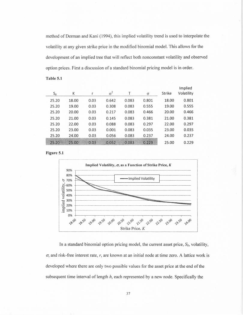
method of Derman and Kani (1994), this implied volatility trend is used to interpolate the

volatility at any given strike price in the modified binomial model. This allows for the

development of an implied tree that will reflect both nonconstant volatility and observed

option prices. First a discussion of a standard binomial pricing model is in order.

Table 5.1

Implied

So K ?

T Strike Volatility (J- (J

25.20 18.00 0.03 0.642 0.083 0.801 18.00 0.801

25.20 19.00 0.03 0.308 0.083 0.555 19.00 0.555

25.20 20.00 0.03 0.217 0.083 0.466 20.00 0.466

25.20 21.00 0.03 0.145 0.083 0.381 21.00 0.381

25.20 22.00 0.03 0.088 0.083 0.297 22.00 0.297

25.20 23.00 0.03 0.001 0.083 0.035 23 .00 0.035

25.20 24.00 0.03 0.056 0.083 0.237 24.00 0.237

25.00 0.03 0.052 0.083 0.229 25.00 0.229

Figure 5.1

90%

80%

b 70%

.~60% ::3 50% ~

'040% >

-0 30% Q)

:.::: 20% c.. .5 10%

Implied Volatility, u, as a Function of Strike Price, K

~ I -Implied Volatility I ~ ~ ~ ~

0% +---.--'r-~--~--~--'---~--.--'--~--~--~

~ ~ ~ ~ ~ ~ ~ ~ ~ ~ ~ ~ ~ ... '0' ... '0 ' ... OJ · ... OJ · "vr::J ' "vr::J ' "v.... "v.... "v"v' "v"v' "v"" "v"" ~.

Strike Price. K

In a standard binomial option pricing model, the current asset price, So, volatility,

cr, and risk-free interest rate, r, are known at an initial node at time zero. A lattice work is

developed where there are only two possible values for the asset price at the end of the

subsequent time interval of length h, each represented by a new node. Specifically the

37

asset price either increases by a known factor u, with a known probability, or decreases

by a known factor d, with a known probability. This pattern continues from each of these

nodes to a set of new nodes at yet another subsequent level. There are a number of

standard binomial models, but for the purpose here we will use the Cox-Ross-Rubenstein

Binomial Model (1979), which will allow for the calculation of future asset prices as well

as the value at time to of an option expiring at time tn. This model will be referred to as

the CRR model from here on. The focus initially will be on determination of future asset

prices, then move to valuing a European call option expiring at In with strike price K = So.

First there is a need to define some of the system parameters for this model and develop

the fundamental mathematical and probabilistic relationships.

Definition 5.1 Risk neutral probability is the probability that an asset price will go up so

that the stock earns the risk-free interest rate. The risk-neutral probability is denoted as

p*.

From the above definition it can be seen that the risk-neutral term in the definition

does not refer to investor preference, but simply to the idea that there is a probability that

an asset price will increase over a given interval of time, h, in a risk-neutral market.

Mathematically this means that for some upward transition factor u and some downward

transition factor d, the following relationship must hold.

Equation 5.1 Sr+h = erhSr = P*USI + (1 - p*)dSI

In other words the expected value of the asset at time t + h is the same as the value of the

asset growing at the risk free rate, r. Solving Equation 5.1 for p* and dividing by the asset

price, SI, gives the following equation for the risk-neutral probability,p*, of an upward

move.

38

e rh -d Equation 5.2 p* =-­

u-d

In order to develop the lattice for a binomial model it is also necessary to determine u and

d. The risk-neutral probability p* addresses the likelihood of an up or down move, but

does not address the magnitude of the move. As a result there is another component of

uncertainty that needs to be incorporated into the binomial model. The eRR model uses

the standard deviation of the continuously compounded return on the asset, otherwise

known as (7, to aid in determining the actual uncertainty in the magnitude of the up and

down factors by which the asset price changes. Since the model is dealing with a time

interval h, the relevant uncertainty is equivalent to e±u...fh. This leads to the following

relationships and values for u and d in the presence of uncertainty for the eRR model.

Now everything necessary to construct a eRR binomial tree is available. The tree

will then be used to obtain the option price over period Tusing k intervals of length h.

This is equivalent to saying that h = Tlk and for the purpose here and clarity of

demonstration, we will let T = 3 years and h = 1 year without loss of generality. In

addition let the asset price at time 0 be So = 100, the risk-free rate r = 2.956% (so that er =

1.03), the initial (and constant) volatility (7= 10%, and the dividend rate be zero (no

dividend payments). For ease of reference consider Figure 5.2 below, where the nodes in

a three period eRR binomial tree will be denoted by the letters A through 1. Using the

references in Figure 5.2, the starting asset price will be SA = So, which was set at 100, the

asset price at time t = I will be SB for an upward move and Sc for a downward move, and

so on for the remaining levels of the tree. Using Equations 5.2 and 5.3 the values of u, d,

39

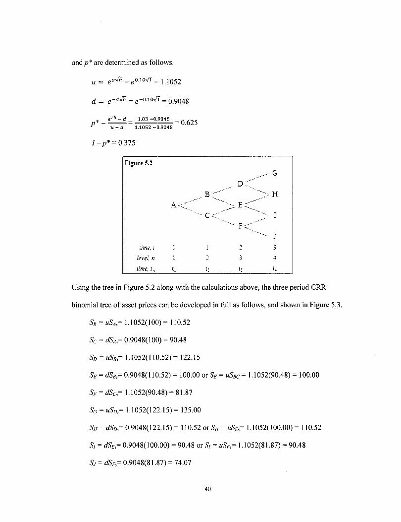
and p* are determined as follows.

d = e-a-/h = e-0.1o.J1 = 0.9048

* = eTh

- d = 1.03 -0.9048 = 0.625 p u - d 1.1052 -0.9048

1-p* = 0.375

Figure ~.1

A <~~~~~._ . .. C

um€. , C

I?VfI, n :2

rim€, l ~ tl t:

3 , ...

Using the tree in Figure 5.2 along with the calculations above, the three period eRR

binomial tree of asset prices can be developed in full as follows, and shown in Figure 5.3.

SB = USA, = 1.1052(100) = 110.52

Sc = dSA,= 0.9048(100) = 90.48

SD = USB,= 1.1052(110.52) = 122.15

SE = dSB,= 0.9048(110.52) = 100.00 or SE = USBC = 1.1052(90.48) = 100.00

SF = dSc,= 1.1052(90.48) = 81.87

SG = USD,= 1.1052(122.15) = 135.00

SH = dSD,= 0.9048(122.15) = 110.52 or SH = USE,= 1.1052(100.00) = 110.52

Sf = dSE,= 0.9048(100.00) = 90.48 or Sf = USF,= 1.1052(81.87) = 90.48

SJ = dSF,= 0.9048(81.87) = 74.07

40

Note that the nature of u and d, which are reciprocals, allows for the lattice style known

as a recombining tree, since there are two ways to calculate intermediate nodes, a fact

that agrees nicely with the binomial nature of the tree. So under the eRR binomial asset

model, four possible values of the asset at time t = 3 are possible as shown in Figure 5.3,

but thus far only the possible asset prices as determined by u and d, and not their

likelihoods have been determined.

Figure 5.3

74.07 ...

...

C; t;

Since the volatility is constant at 10%, and the values of u and d depend only on a

and h, it follows that the probability of an upward move from any node at any level of the

tree is also constant, namely p* = 0.625. Similarly then the probability of a downward

move from any node at any level of the tree is constant, namely 1-p* = 0.375. So the

probability of reaching the top node at level n is simple (p*r and the probability of

reaching the bottom node is (1-p*r. Similarly then to reach the/h node below the top at

any level of the tree, exactly j downward movements are required, and there are n ways to

do so. For example node H is one node below the top node when n = 3, so one downward

movement and two upward movements are required. This lone downward movement can

occur in the transition to level n = 2, level n = 3, or level n = 4. This means that there are

41

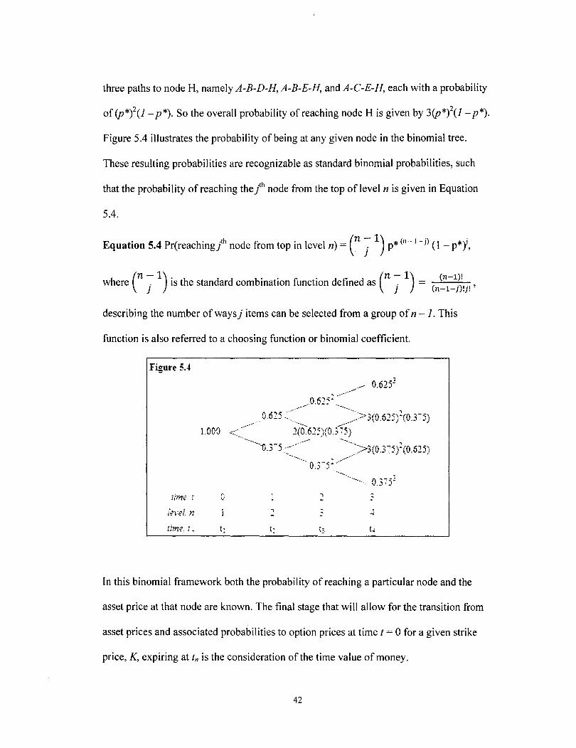
three paths to node H, namely A-B-D-H, A-B-E-H, and A-C-E-H, each with a probability

of (p*iu- p*). So the overall probability of reaching node H is given by 3(p*iu- p*).

Figure 5.4 illustrates the probability of being at any given node in the binomial tree.

These resulting probabilities are recognizable as standard binomial probabilities, such

that the probability of reaching the /h node from the top of level n is given in Equation

5.4.

Equation 5.4 Pr(reaching/h node from top in level n) = (n j 1) p* (n-l-j) (1- p*Y,

where (n ~ 1) is the standard combination function defined as (n ~ 1) = ( (n-l~; . , J J n-l-] !]!

describing the number of ways j items can be selected from a group of n - 1. This

function is also referred to a choosing function or binomial coefficient.

Figure 504

1.000

0.3":'53

ibn,; j ;, .... 3 v -

kv?l n .... : .1 - -.

jim? i. t1 t: t: [ ..

In this binomial framework both the probability of reaching a particular node and the

asset price at that node are known. The final stage that will allow for the transition from

asset prices and associated probabilities to option prices at time t = 0 for a given strike

price, K, expiring at tn is the consideration of the time value of money.

42

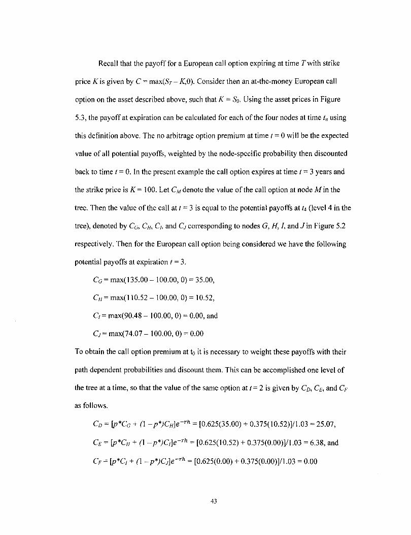
Recall that the payoff for a European call option expiring at time Twith strike

price K is given by C = max(ST - K,O). Consider then an at-the-money European call

option on the asset described above, such that K = So. Using the asset prices in Figure

5.3, the payoff at expiration can be calculated for each of the four nodes at time In using

this definition above. The no arbitrage option premium at time 1= 0 will be the expected

value of all potential payoffs, weighted by the node-specific probability then discounted

back to time t = O. In the present example the call option expires at time 1= 3 years and

the strike price is K = 100. Let C M denote the value of the call option at node M in the

tree. Then the value of the call at I = 3 is equal to the potential payoffs at 14 (level 4 in the

tree), denoted by Ce, CH, C/, and Cj corresponding to nodes G, H, I, and J in Figure 5.2

respectively. Then for the European call option being considered we have the following

potential payoffs at expiration 1=3.

Ce = max(135.00 - 100.00, 0) = 35.00,

CH = max(11 0.52 - 100.00, 0) = 10.52,

C/ = max(90.48 - 100.00, 0) = 0.00, and

Cj = max(74.07 - 100.00, 0) = 0.00

To obtain the call option premium at to it is necessary to weight these payoffs with their

path dependent probabilities and discount them. This can be accomplished one level of

the tree at a time, so that the value of the same option at t= 2 is given by CD, CE, and CF

as follows.

CD = fp*Ce + (1 - p*)CH]e-rh = [0.625(35.00) + 0.375(10.52)]/1.03 = 25.07,

CE = fp*CH + (1 - p*)C/]e-rh = [0.625(10.52) + 0.375(0.00)]/1.03 = 6.38, and

CF = fp*C/ + (1 - p*)Cj]e-rh = [0.625(0.00) + 0.375(0.00)]/1.03 = 0.00

43

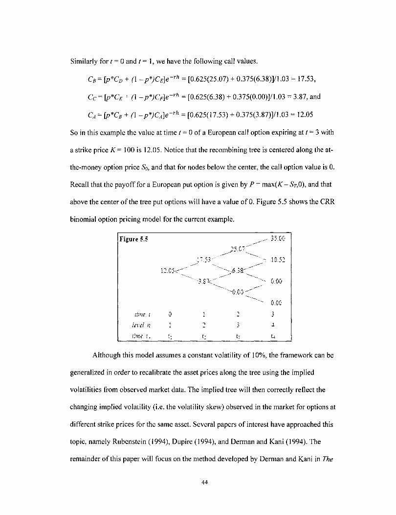
Similarly for t == 0 and t == 1, we have the following call values.

CB == fp*CD + (l - p*)CE]e-rh == [0.625(25.07) + 0.375(6.38)]11.03 = 17.53,

Cc = fp*CE + (l - p*)CF]e-rh == [0.625(6.38) + 0.375(0.00)]/1.03 == 3.87, and

CA == fp*CB + (l - p*)CA]e-rh == [0.625(17.53) + 0.375(3.87)]/1.03 == 12.05

So in this example the value at time t == 0 of a European call option expiring at t == 3 with

a strike price K== 100 is 12.05. Notice that the recombining tree is centered along the at-

the-money option price So, and that for nodes below the center, the call option value is O.

Recall that the payoff for a European put option is given by P == max(K - Sr,O), and that

above the center of the tree put options will have a value ofO. Figure 5.5 shows the eRR

binomial option pricing model for the current example.

Figure ~.~

J"--~

... - f',""'-----),1 ... ' ,

:-:.53---- 10.52 1 ... C'l,----· - -. - ~~-'-.

·---··-->6.3&-~~:~------. 0.00

-'--0.00 -""-

- 0.00

rt?ne. j 0

hl'd ;~ ., -

r}m; r . [; t: t ..

Although this model assumes a constant volatility of 10%, the framework can be

generalized in order to recalibrate the asset prices along the tree using the implied

volatilities from observed market data. The implied tree will then correctly reflect the

changing implied volatility (i.e. the volatility skew) observed in the market for options at

different strike prices for the same asset. Several papers of interest have approached this

topic, namely Rubenstein (1994), Dupire (1994), and Derman and Kani (1994). The

remainder of this paper will focus on the method developed by Derman and Kani in The

44

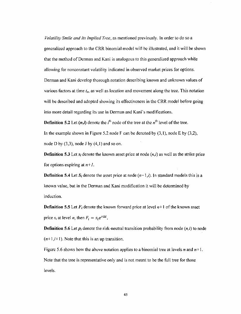
Volatility Smile and Its Implied Tree, as mentioned previously. In order to do so a

generalized approach to the CRR binomial model will be illustrated, and it will be shown

that the method of Derman and Kani is analogous to this generalized approach while

allowing for nonconstant volatility indicated in observed market prices for options.

Derman and Kani develop thorough notation describing known and unknown values of

various factors at time tn, as well as location and movement along the tree. This notation

will be described and adopted showing its effectiveness in the CRR model before going

into more detail regarding its use in Derman and Kani's modifications.

Definition 5.2 Let (n,l) denote the ith node of the tree at the nth level of the tree.

In the example shown in Figure 5.2 node F can be denoted by (3,1), node E by (3,2),

node D by (3,3), node J by (4,1) and so on.

Definition 5.3 Let Si denote the known asset price at node (n,i) as well as the strike price

for options expiring at n+ 1.

Definition 5.4 Let Si denote the asset price at node (n+ l,i). In standard models this is a

known value, but in the Derman and Kani modification it will be determined by

induction.

Definition 5.5 Let Fi denote the known forward price at level n+ 1 of the known asset

price Si at level n, then Fi = Sierllt.

Definition 5.6 Let Pi denote the risk-neutral transition probability from node (n,i) to node

(n+ 1 ,i+ 1). Note that this is an up transition.

Figure 5.6 shows how the above notation applies to a binomial tree at levels nand n+ 1.

Note that the tree is representative only and is not meant to be the full tree for those

levels.

45

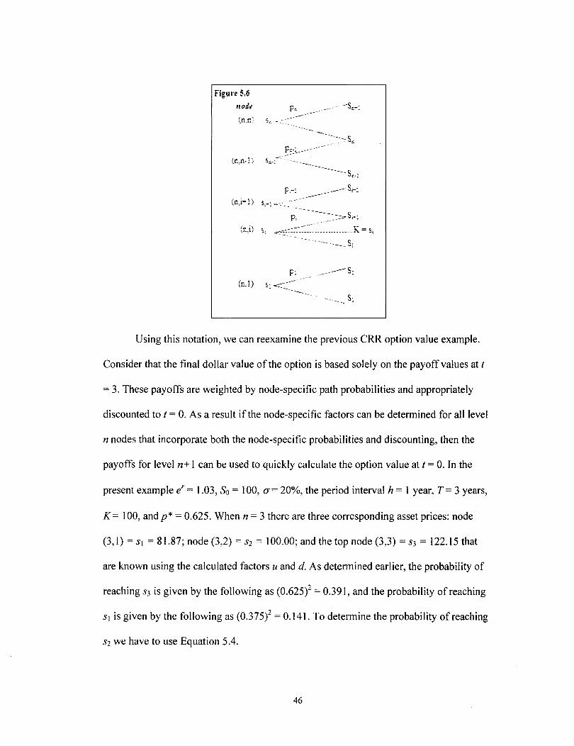
Figure 5.6 nodI?

(r.,n·l}

(n,i-1) S,-!

~.~-~--, __ ~- OJ!,

p, -==_-_~~~-~S'-l (n,i) ~, ~-:<:-.-~-=:~ .. ~~ .. _ ..... ___ K = ;;

t:. ~,

F: S: (1'.,1) >;

S:

Using this notation, we can reexamine the previous CRR option value example.

Consider that the final dollar value of the option is based solely on the payoff values at t

= 3. These payoffs are weighted by node-specific path probabilities and appropriately

discounted to t = O. As a result if the node-specific factors can be determined for all level

n nodes that incorporate both the node-specific probabilities and discounting, then the

payoffs for level n+ 1 can be used to quickly calculate the option value at t = O. In the

present example er = 1.03, So = 100, (]"= 20%, the period interval h = 1 year, T= 3 years,

K = 100, and p* = 0.625. When n = 3 there are three corresponding asset prices: node

(3,1) =SI = 81.87; node (3,2) =S2 = 100.00; and the top node (3,3) =S3 = 122.15 that

are known using the calculated factors u and d. As determined earlier, the probability of

reaching S3 is given by the following as (0.625i = 0.391, and the probability of reaching

SI is given by the following as (0.375i = 0.141. To determine the probability of reaching

S2 we have to use Equation 5.4.

46

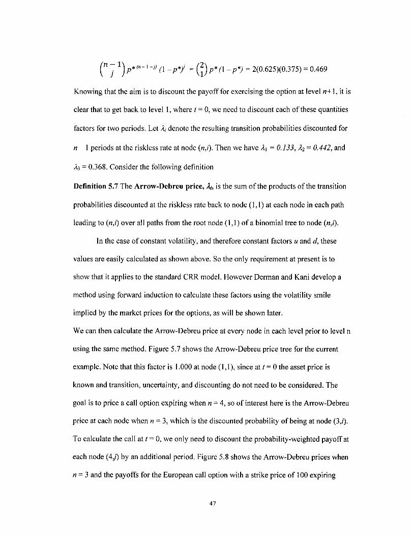
(n j 1) p* (n- I-j) (1 - p*j = (i) p* (1 - p*) = 2(0.625)(0.375) = 0.469

Knowing that the aim is to discount the payoff for exercising the option at level n+ 1, it is

clear that to get back to level 1, where t = 0, we need to discount each of these quantities

factors for two periods. Let Ai denote the resulting transition probabilities discounted for

n- 1 periods at the riskless rate at node (n,i). Then we have AI = 0.133, .12 = 0.442, and

.13 = 0.368. Consider the following definition

Definition 5.7 The Arrow-Debreu price, ..1.;, is the sum of the products of the transition

probabilities discounted at the riskless rate back to node (l, 1) at each node in each path

leading to (n,i) over all paths from the root node (l, 1) of a binomial tree to node (n,i).

In the case of constant volatility, and therefore constant factors u and d, these

values are easily calculated as shown above. So the only requirement at present is to

show that it applies to the standard CRR model. However Derman and Kani develop a

method using forward induction to calculate these factors using the volatility smile

implied by the market prices for the options, as will be shown later.

We can then calculate the Arrow-Debreu price at every node in each level prior to level n

using the same method. Figure 5.7 shows the Arrow-Debreu price tree for the current

example. Note that this factor is 1.000 at node (1,1), since at t = 0 the asset price is

known and transition, uncertainty, and discounting do not need to be considered. The

goal is to price a call option expiring when n = 4, so of interest here is the Arrow-Debreu

price at each node when n = 3, which is the discounted probability of being at node (3,i).

To calculate the call at t = 0, we only need to discount the probability-weighted payoff at

each node (4J) by an additional period. Figure 5.8 shows the Arrow-Debreu prices when

n = 3 and the payoffs for the European call option with a strike price of 100 expiring

47

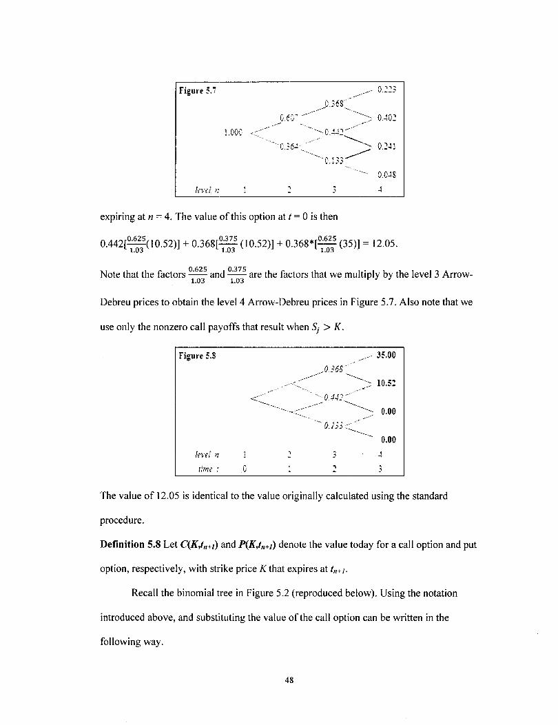
Figure 5.i ~'. -.." ... __ .-- 1.J. __ J

1.1)00

, ) j

expiring at n = 4. The value of this option at t = 0 is then

0.442[°·625(10.52)] + 0.368[°.375 (10.52)] + 0.368*[°·625 (35)] = 12.05. 1.03 1.03 1.03

Note that the factors 0.625 and 0.375 are the factors that we multiply by the level 3 Arrow-1.03 1.03

Debreu prices to obtain the level 4 Arrow-Debreu prices in Figure 5.7. Also note that we

use only the nonzero call payoffs that result when Sj > K.

Figure 5.S / ___ 35.00

0368-

10.51

0.233

0.00 , )

, )

The value of 12.05 is identical to the value originally calculated using the standard

procedure.

Definition 5.8 Let C(K,tn+l) and P(K,tn+l) denote the value today for a call option and put

option, respectively, with strike price K that expires at tn+ /.

Recall the binomial tree in Figure 5.2 (reproduced below). Using the notation

introduced above, and substituting the value of the call option can be written in the

following way.

48

Figure 5.2 G

D ., ..

B H .l..<' E

~.,_T--. .. -.. C .. ..

F J

::n:.r. i

livd n ~

:}1?U 1. t· t: t; t.

The resulting summation formula describing this relationship is given as Equation 5.5. In

general the length of the period h is also the change in t and can be written as M.

Now consider the binomial model proposed by Derman and Kani. The asset price

at t = 0 and the option prices are known from the market data. Using the Black-Scholes

formula the implied volatilities can be calculated, resulting in a relationship between the

strike price and volatility (volatility skew) that allows for option prices to be interpolated

for any strike price. Assuming that the initial volatility is that for an at-the-money

European call option, the implied tree is developed starting at node (1,1) and using

induction the implied asset prices at each node in the tree are calculated. The result being

a binomial tree that correctly reflects observed option prices in the market and the

volatility skew. The known transition probabilities are risk neutral, which means that the

expected value of the asset at any node (n,i) in the next period is equal to the forward

price, resulting in the following equations.

Equation 5.6 F; = PiS;+l+(l - p[)S;

Solving Equation 5.6 for pi results in the following.

49

F--S­Equation 5.7 pi = ! !

Si+1- Si

In the eRR binomial model, pi was constant, but here it can be seen that it depends on

the position in the tree. This makes sense because pi is defined to be the probability of an

upward transition from a node for a given volatility, and in the modified tree the volatility

is known to be changing.

Since Derman and Kani are using a model that is anchored at level n with known

forward prices, known implied volatilities, and known Arrow-Debreu prices, the

following equation reflects the value of a call option with strike price K expiring at Ind.

Since the strike price K is set equal to Si, the known asset price at (n,i), consider what

happens with regard to the transition to the first up node Si+ I. The above summation can

be simplified by multiplying Equation 5.8 by erl then examining the summation term by

term beginning with the first in-the-money up move, in other words when} = i, then the

index of the remaining summation will run from} = i+ I to} = n as shown below.

Equation 5.9

Notice that the first term in Equation 5.9 is the contribution of the overall value

resulting from the first in-the-money option, and the remaining terms are equivalent to

Equation 5.8 with a change of index described above. Now consider the sum given by the

second and third terms in Equation 5.9, specifically

50

By distributing we have

By collecting like terms and applying Equation 5.6, we have

Similar results follow for the remaining terms up to} = n. This yields the following

overall results.

Since the forward prices and option prices, Fi and the C(Si,!n+l) respectively, are known,

we can solve 5.6 and 5.10 simultaneously for Si+l and pi with the following result.

Using this relationship for call options, the implied asset prices, 8;, and risk­

neutral probabilities, Pj, for each node in upper portion of the binomial tree at the (n+ l)th

level can be completed, assuming there is a value Si for an initial node. At any given

(n+ l)th level of the tree, the number of nodes is either even or odd. Based on the

centering condition described before, if the (n+ l)th level has an odd number of nodes, the

Si used will be the central node of the tree (i.e. the CRR spot price). Due to the

recombining nature of the tree and the fact that the central node in an odd level is equal to

the CRR spot price, the nodes above can be calculated using Equations 5.7 and 5.11.

When the (n+ l)th level is even, Si will be the node just below the center ofthe tree and

Si+l will be the node just above the center, where i=(n+ 1)12. Again based on the

51

centering condition, the eRR spot price S; is the geometric mean of S; and SH1, namely

2

Si = ~. Substituting this result into Equation 5.11 gives the following result for Si+1

calculating the asset price at node (n+ I,~) where n is even. 2

Once the upper half of the tree at the (n+ I yh level has been completed using call

prices, then we complete the lower half of the tree in a similar manner using the known

put prices. Recall that the payoff at time T for a European put option expiring at T with

strike price K is given by P = max(K - S[,O). So the asset price at the node (n+ 1,i) in the

(n+ I )th level can be determined from the known asset price at the known upper node

(n+ I,i+ I) using Equation 5.13. The basis of Equation 5.13 is analogous to that of

Equation 5.12 and can be found in the appendix.

Using the above methods, the implied tree of asset prices can be constructed node by

node down to i= lthat accurately represents the volatility skew and market option prices

at each level of the tree.

To demonstrate this we will construct a theoretical example. Suppose option

prices on a stock with current price 50 are collected and the implied volatilities are

calculated. Furthermore suppose that the resulting volatility smile indicates that the at-

the-money options have an implied volatility of 0.15, and that analysis of the smile

indicates the relationship between implied volatility and strike price is as follows. For

every two dollar change in strike price, the implied volatility changes by 0.004. When the

strike price K is below the current price then the volatility increases and when K is above

52

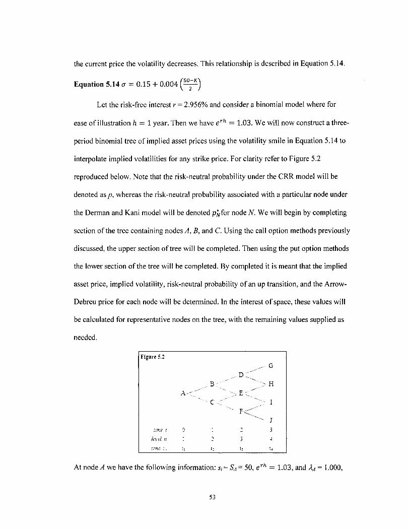
the current price the volatility decreases. This relationship is described in Equation 5.14.

(SO-K) Equation 5.14 a = 0.15 + 0.004 -2-

Let the risk-free interest r = 2.956% and consider a binomial model where for

ease of illustration h = 1 year. Then we have eTh = 1.03. We will now construct a three-

period binomial tree of implied asset prices using the volatility smile in Equation 5.14 to

interpolate implied volatilities for any strike price. For clarity refer to Figure 5.2

reproduced below. Note that the risk-neutral probability under the eRR model will be

denoted as p, whereas the risk-neutral probability associated with a particular node under

the Derman and Kani model will be denoted p~for node N. We will begin by completing

section of the tree containing nodes A, B, and C. Using the call option methods previously

discussed, the upper section of tree will be completed. Then using the put option methods

the lower section of the tree will be completed. By completed it is meant that the implied

asset price, implied volatility, risk-neutral probability of an up transition, and the Arrow-

Debreu price for each node will be determined. In the interest of space, these values will

be calculated for representative nodes on the tree, with the remaining values supplied as

needed.

Figure 5.1

B "., H ,..,.----

00. 0·0 c .. :~

J ji},~::f l ::: ,

~ -iel:i l 11

, J ..1 -

r:m,' l t, t: t; t.

At node A we have the following information: Si = SA = 50, e Th = 1.03, and itA = 1.000,

53

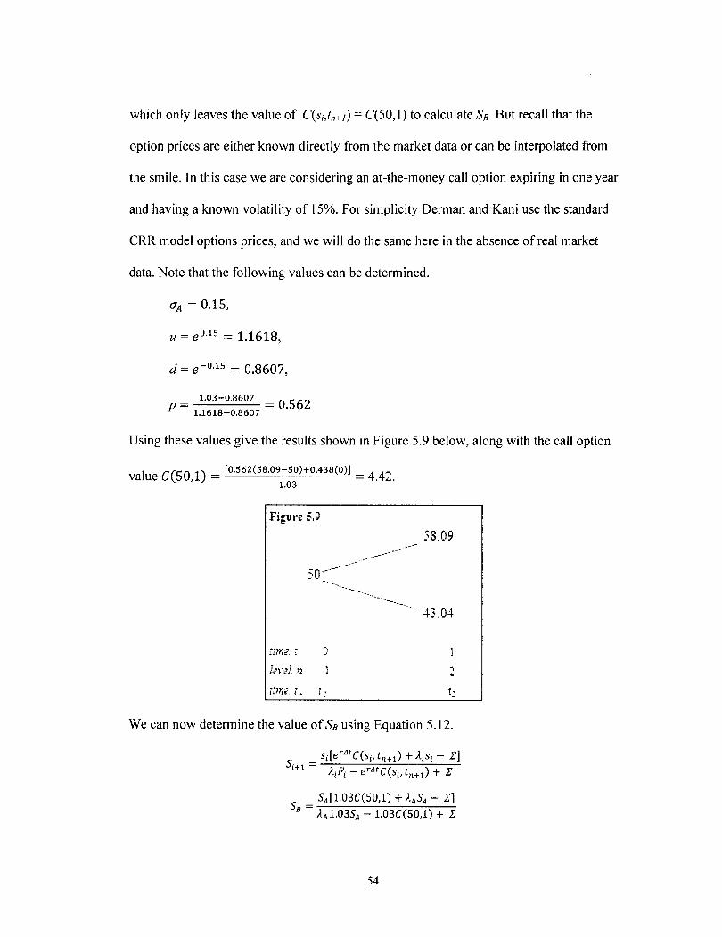
which only leaves the value of C(Si,tn+l) = C(50, 1) to calculate SB. But recall that the

option prices are either known directly from the market data or can be interpolated from

the smile. In this case we are considering an at-the-money call option expiring in one year

and having a known volatility of 15%. For simplicity Derman and Kani use the standard

eRR model options prices, and we will do the same here in the absence of real market

data. Note that the following values can be determined.

aA = 0.15,

u = eO.15 = 1.1618,

d = e-O.15 = 0.8607,

= 1.03-0.8607 = 0.562 P 1.1618-0.8607

Using these values give the results shown in Figure 5.9 below, along with the call option

value C(50,1) = [0.562(58.09-50)+0.438(0)) = 4.42. 1.03

Figure 5.9

----

-----

-",---

--... --

j.'m"c j " c ..

l;l.:?l 1'1

r:n-;=,: , , , .'

58.09

43.04

... -t:

We can now determine the value of SB using Equation 5.12.

54

Since there are no nodes above node B at n = 2, the summation terms are zero and we

have.

50[1.03(4.42) + 1.000(50)] S8 = 1.000[1.03(50)] -1.03(4.42) = 58.09

Using the centering condition for even levels, we have the following for Sc.

Sl (50)2 Sc = S8 = 58.09 = 43.04

Now applying Equation 5.7 we can determine the value ofpAas follows.

• FA - Sc 51.50 - 43.04 PA = S8 - Sc = 58.09 - 43.04 = 0.562

In general we need to find Si+ I, Sj, and F j in order to calculate pi, but notice at the initial

node of the tree it turns out that all values are the same as in the eRR model. For

thoroughness we stuck to the model developed by Derman and Kani even for the first

period of the tree.

We now move on to n = 3 and determine the values associated with nodes D and E

using the values for node B and Equation 5.11.

Because of the centering condition where the center of the implied tree is the same as the

standard eRR model, we know the implied asset value SE = 50. And since node D is the

highest node for n = 3, the summation term is zero. We need to calculate the value of the

call option C(58.09,2), and again this will be done using the standard eRR model, but

with the volatility (JB based on the volatility smile. Now we have the following values

and can use them to determine the call value as shown in Figure 5.10 below.

55

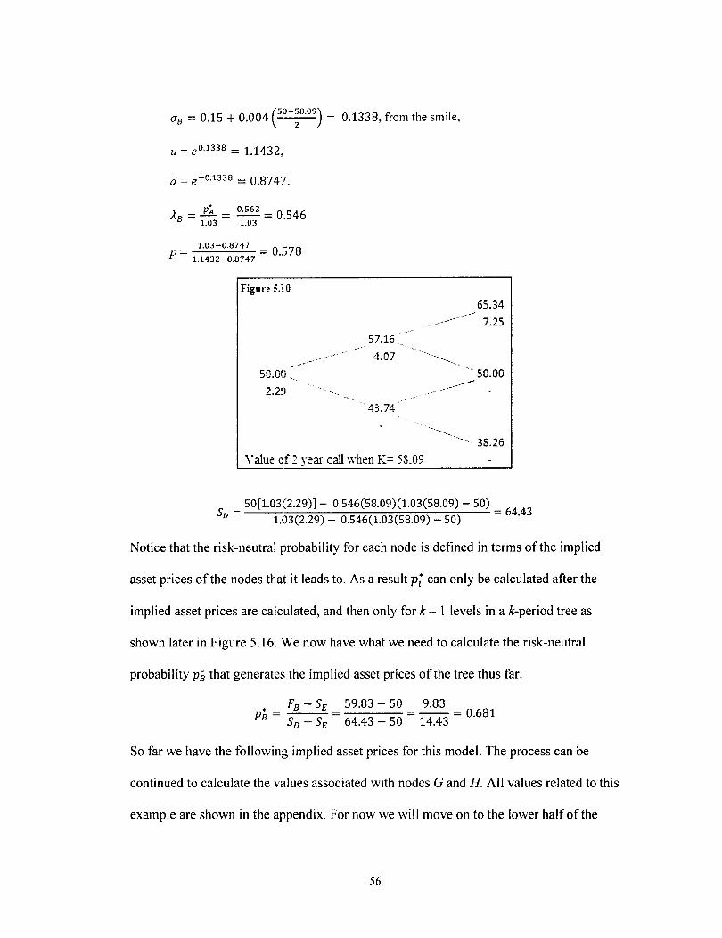
(Js = 0.15 + 0.004 CO-~8.09) = 0.1338, from the smile,

u = eO. 1338 = 1.1432,

d = e-O.1338 = 0.8747,

its = PA = 0.562 = 0.546 1.03 1.03

= 1.03-0.8747 = 0.578 p 1.1432-0.8747

Figure 5.10

50.00 2.29

57.16

4.07

\·alue of2 year call \vhen K= 58_09

65.34

7.25

50.00

38.26

50[1.03(2.29)] - 0.546(58.09)(1.03(58.09) - 50) S = = 6443

D 1.03(2.29) - 0.546(1.03(58.09) - 50) .

Notice that the risk-neutral probability for each node is defined in terms of the implied

asset prices of the nodes that it leads to. As a result pi can only be calculated after the

implied asset prices are calculated, and then only for k - 1 levels in a k-period tree as

shown later in Figure 5.16. We now have what we need to calculate the risk-neutral

probability pi, that generates the implied asset prices of the tree thus far.

• Fs - SE 59.83 - 50 9.83 Ps = SD - SE = 64.43 - 50 = 14.43 = 0.681

So far we have the following implied asset prices for this model. The process can be

continued to calculate the values associated with nodes G and H. All values related to this

example are shown in the appendix. For now we will move on to the lower half of the

56

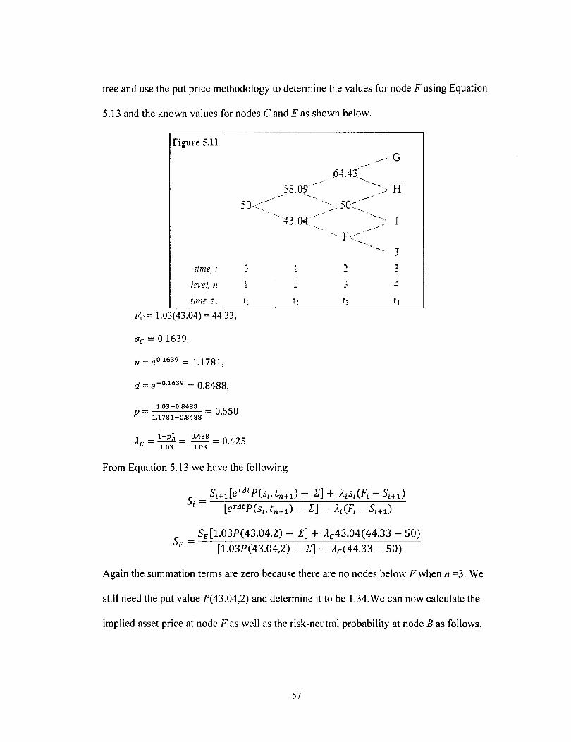
tree and use the put price methodology to determine the values for node F using Equation

5.13 and the known values for nodes C and E as shown below.

Figure ~.ll

Fe = 1.03(43.04) = 44.33,

O'c = 0.1639,

u = eO.1639 = 1.1781,

d = e-O.1639 = 0.8488,

= 1.03-0.8488 = 0.550 p 1.1781-0.8488

AC = 1-PA = 0.438 = 0.425 1.03 1.03

From Equation 5.13 we have the following

t: t:;

_---- G

J

t+

Sd1.03P(43.04,2) - r] + Ac43.04(44.33 - 50) SF = [1.03P(43.04,2) - r] - Ac(44.33 - 50)

Again the summation terms are zero because there are no nodes below Fwhen n =3. We

still need the put value P(43.04,2) and determine it to be 1.34.We can now calculate the

implied asset price at node F as well as the risk-neutral probability at node B as follows.

57

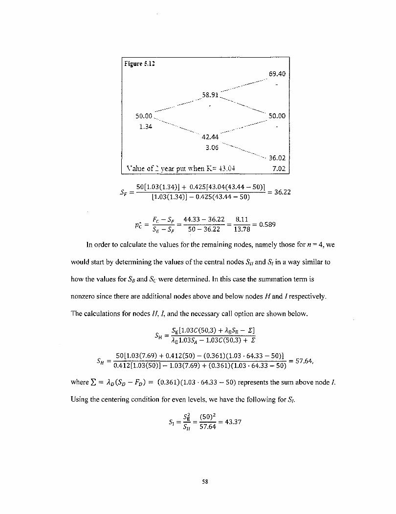
Figure 5.12

69.40

----------58.91~~---

50.00

1.34

----~

.-~---------~------. 50.00

42.44

3.06

Value of 1 year put , .... hen K= 43.04

-­_----..r--

36.02

7.02

50[1.03(1.34)] + 0.425[43.04(43.44 - 50)] SF = [1.03(1.34)] _ 0.425(43.44 _ 50) = 36.22

• Fe - SF 44.33 - 36.22 8.11 Pc = SE - SF = 50 - 36.22 = 13.78 = 0.589

In order to calculate the values for the remaining nodes, namely those for n = 4, we

would start by determining the values of the central nodes SH and SI in a way similar to

how the values for S8 and Sc were determined. In this case the summation term is

nonzero since there are additional nodes above and below nodes H and I respectively.

The calculations for nodes H, I, and the necessary call option are shown below.

Sd1.03C(50,3) + AESE - 1'] SH = ----------

AE1.03SA - 1.03C(50,3) + l'

50[1.03(7.69) + 0.412(50) - (0.361)(1.03 . 64.33 - 50)] SH = 0.412[1.03(50)] _ 1.03(7.69) + (0.361)(1.03 .64.33 _ 50) = 57.64,

where L = AD(SD - FD) = (0.361)(1.03·64.33 - 50) represents the sum above node I.

Using the centering condition for even levels, we have the following for SI.

S~ (50)2 SI = -S = -5 6 = 43.37

H 7. 4

58

Figure ~.l3

50.00 "

7.69

58.09,

12.22

43.04'

2.41

\ 'a!lle of 3 year call when ~= 50

67.49'-

18.95

50.CO ..... ..

':.42

37.04

78.42 .. " ' 28.42

.. 58.09

8.09

, 43.04

31.83

Now applying Equation 5.7 we can determine the value ofp;as follows.

• FE - 5) 51.50 - 43.37 PE = 5

H - 5) = 57.64 _ 43.37 = 0.562

Now the values for nodes G and J can be calculated. Below is a demonstration of the

calculation for node J only using out values in a way similar to that for node F.

s _ _ SI_[1--"..0_3_P_(3_6_.2_2_,3_)_-_E_l-.,+,,--A_F 3_6_.2_2_(1_,0_3_'_3_6,_2_2 _-_4_3_.3_7) J - [1.03P(36,22,3) - El - AF(1.03 ' 36,22 - 43.37)

Figure ~.}.t

50.00

0.61

59.7L", --.-

85.17

··~·59.71

50.00

41.87 '. 41.87

1.37 '"

\'alue 01'3 year put when h= 36,22

". 35.05

3.0t" ",

"-. 29.35

6.87

The above figure shows the value of P(36.22,3). Again the summation terms are zero

since we are at the bottom of the tree.

59

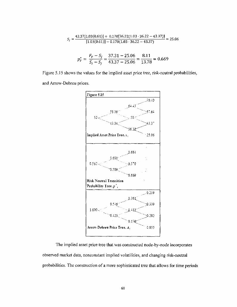
43.37[1.03(0.61)] + 0.170[36.22(1.03·36.22 - 43.37)] S = = 25.06

J [1.03(0.61)] - 0.170(1.03·36.22 - 43.37)

• Fp - Sf 37.31 - 25.06 8.11 PF = SI - Sf = 43.37 - 25.06 = 13.78 = 0.669

Figure 5.15 shows the values for the implied asset price tree, risk-neutral probabilities,

and Arrow-Debreu prices.

Figure 5.15

SD<----

--~·~:43.3: --~-3 6 .ll~~:~---~ ..

Implied :\sset Price Tree, I j

96S1 '.'.-..

Risk :'1-eutral Transition

Probability Tree,p·J

1.!){}D<·~ .~--'--

---0 ~25:::

.a.36(

:\l'I'ow-Debreu Price Tree, J. j

~::::{l.3 3 9

The implied asset price tree that was constructed node-by-node incorporates

observed market data, nonconstant implied volatilities, and changing risk-neutral

probabilities. The construction of a more sophisticated tree that allows for time periods

60

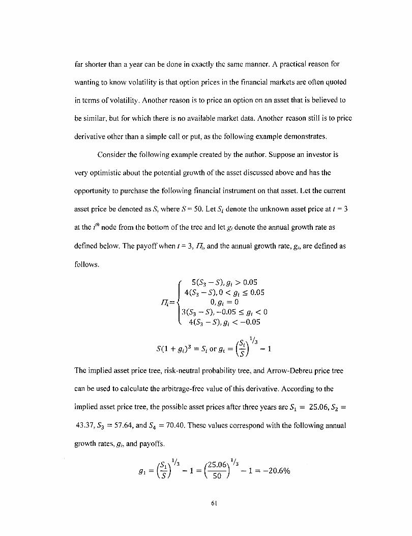
far shorter than a year can be done in exactly the same manner. A practical reason for

wanting to know volatility is that option prices in the financial markets are often quoted

in terms of volatility. Another reason is to price an option on an asset that is believed to

be similar, but for which there is no available market data. Another reason still is to price

derivative other than a simple call or put, as the following example demonstrates.

Consider the following example created by the author. Suppose an investor is

very optimistic about the potential growth of the asset discussed above and has the

opportunity to purchase the following financial instrument on that asset. Let the current

asset price be denoted as S, where S = 50. Let 5 i denote the unknown asset price at t = 3

at the /h node from the bottom of the tree and let gi denote the annual growth rate as

defined below. The payoff when t = 3, /Z, and the annual growth rate, gi, are defined as

follows.

5(53 - 5), 9i > 0.05 4(53 - 5),0 < 9i ~ 0.05

Il;.= 0,9i = 0 3(53 - 5), -0.05 ~ 9i < 0

4(53 - 5), 9i < -0.05

The implied asset price tree, risk-neutral probability tree, and Arrow-Debreu price tree

can be used to calculate the arbitrage-free value of this derivative. According to the

implied asset price tree, the possible asset prices after three years are 51 = 25.06,52 =

43.37,53 = 57.64, and 54 == 70.40. These values correspond with the following annual

growth rates, 9i, and payoffs.

(Sl)lh (2S.06)lh

91 = S - 1 = 50 - 1 = -20.6%

61

1ft =4(25.06 - 50)= - 99.76

(S2)lh (43.37)lh

92 =·s - 1 = 5() - 1 = -4.6%

]]2=3(43.37 - 50)= -19.89

(S3)lh (57.64)lh

93 = S -1 = 5() -1 = 4.9%

]]3=4(57.64 - 50) = 30.56

(S4)lh (70.40)lh

94 = S - 1 = 5() - 1 = 12.1%

]]4=5(70.40 - 50) = 102

We now use the tree to calculate the value today of this instrument. Refer to Figure 5.16

below.

Figure 5.16

<. ,,' ,v-.-.:!

Implied Asset Prict Tree, ,; -.~~ 06

OSSl

·O.~S9.

Risk:-; tutral Transition

Probabili~' Tree,p',

1.000

.S.5S!

·--·~.569

"D.l:C./

Arrow-Debl'eu Price Tree. )., O.O~~

62

n. 9:

:02 l2.P"

3056 ':9%

-:9.89 .4.6%

-9976 -20.6;,

We can use the payoffs at t = 3, the Arrow-Debreu prices at n = 3, the risk-neutral

transition probabilities for moving from n =3 to n = 4, and the risk free rate r =2.956% to

determine the price today, flo, the derivative as follows.

n1~A1- pF) = -99.76(0.170)(0.331) = -5.61

n 2 [AFP; + ,1£(1- p~)] = -19.89[(0.170)(0.669) + (0.412)(0.430)] = -5.79

n3[A£P~ + AD (1 - p~)]= 30.56[(0.412)(0.570) + (0.361)(0.316)] = 10.66

n4ADP~ = 102[(0.361)(0.684)] = 25.19

no = -5.61-5.79+10.66+25.19 == ~ = 23.74 1~3 L03

In summary, although the popular Black-Scholes formula is widely used and in

many cases an accurate representation of financial market activity, it makes some

assumptions that are contrary to the observed market data. The assumption of constant

volatility across strike prices is one such assumption. However since the Black-Scholes

framework is in fact very robust, slight modifications to existing discrete time models

allow for the accurate modeling of real market dynamics and more sophisticated

derivative pricing. Since the continuous Black-Scholes formula is the limiting case of the

standard discrete models as n~ 00 and h ~ 0, the discrete time modifications are good

proxies and can easily be adjusted to accommodate less conventional payoff

arrangements as demonstrated here.

63

REFERENCES

[1] Arrow, K. and Gerard Debreu, 1954, Existence of General Equilibrium for a Competitive Economy, Econometrica Volume 22, No.3, 265-290.

[2] Baxter, M.W., and A. J. O. Rennie, 1996 Financial Calculus: An Introduction to Derivative Pricing, Cambridge University Press, New York.

[3] Bjork, T., 1998 Arbitrage Theory in Continuous Time, Oxford University Press, New York.

[4] Black, F. and M. Scholes, 1973 The Pricing of Option and Corporate Liabilities, The Journal of Political Economy, Vol. 81, No.3, 637-654.

[5] Bookstaber, Richard M., 1981 Option Pricing and Strategies in Investing, Addison­Wesley Publishing Company, Inc., Phillipines.

[6] Bru, B., P. Crepel, J. Courtault, Y. Kabanov, A. Le Marchand, and I. Lebon, 2000 Louis Bachelier: On the Centenary of Theorie de la Speculation, Mathematical Finance, Vo1.10, No.3 (July 2000), 341-353.

[7] <;etin, U., R. Jarrow, and P. Protter, 2004 Liquidity Risk and Arbitrage Pricing Theory, Finance and Stochastics 8 311-34 L

[8] <;etin, U., R. Jarrow, P. Protter, and M. Warachka, Option Pricing with Liquidity Risk, working paper, Wharton-SMU Research Center of Singapore Management University, http://www.research.smu.edu.sg/or/pdfs/Mitch _ LiquidityOptions.pdf

[9] Cox,1. C., Ross, S. A., and Rubenstein, M., 1979, Option Pricing: A Simplified Approach, Journal of Financial Economics, 7(3), 229 - 263.

[10] Derman, Emanuel and Kani, Iraj, Riding on the Smile, RISK, 7 (February 1994),32-39.

[11] Duffie, D., 1. Pan, K. Singleton. 2000. Transform Analysis and Option Pricing for Affine Jump-Diffusions .. Econometrica 68 1343-1376.

[12] Dupire, Bruno, Pricing with a Smile, RISK, 7 (January 1994), 18-20.

[13] Fama, E.F., L. Fisher, M.e. Jensen, and R. Roll 1969 The Adjustment of Stock Prices to New Information, International Economic Review, Vol. 10.

64

[14] Hull, J.c., 2000 Options, Futures, & Other Derivatives (Fourth Edition), Prentice Hall, Upper Saddle River, New Jersey.

[15] Hull, J.c., 2002 Fundamentals of Futures and Options Markets, Pearson Education, Delhi.

[16] Hull, J., A. White. 1987. The Pricing of Options on Assets with Stochastic Volatilities. Journal of Finance, 42, 281-300.

[17] Jackel, P., 2002 Monte Carlo Methods in Finance, John Wiley and Sons, New York.

[18] Kendall, M.G., The Analysis of Economic Time-Series-Part I: Prices, Journal of the Royal Statistical Society. Series A (General), Vol. 116, No.1 (1953), pp. 11-34.

[19] Leland, H.E., 1984 Option Pricing and Replication with Transactions Costs, http://haas.berkeley.edu/finance/WP/rpf144.pdf

[20] Mahler, H. C., 2007, Mahler's Guide to Financial Economics, Georgia State University, J. Mack Robinson College of Business.

[21] McDonald, Robert L., 2006 Derivatives Markets (Second Edition), Pearson Education, Boston, MA

[22] Merton, R.C., 1990 Continuous-Time Finance, Basil Blackwell Inc., Cambridge, MA.

[23] O'Hara, M., 1995 Market Microstructure Theory, Blackwell Publishers, Cambridge, MA.

[24] Poon, Ser-Huang and Granger, Clive W. J., Forecasting Volatility in Financial Markets: A Review, Journal of Economic Literature, Volume XLI, (June 2003), pp. 478 - 539.

[25] Protter, P., 2001 A Partial Introduction to Financial Asset Pricing Theory, Stochastic Processes and their Applications, 91, 169-203.

[26] Protter, P. and R. Jarrow, 2004 A Short History of Stochastic Integration and Mathematical Finance: The Early Years, 1880-1970, In The Herman Rubin Festschrift, IMS Lecture Notes 45; 75-91.

[27] Rubenstein, Mark, Implied Binomial Trees, Journal of Finance, July, 1994.

[28] Shreve, S.E., 2004 Stochastic Calculus for Finance 1: The Binomial Asset Pricing Model, Springer-Verlag, New York.

65

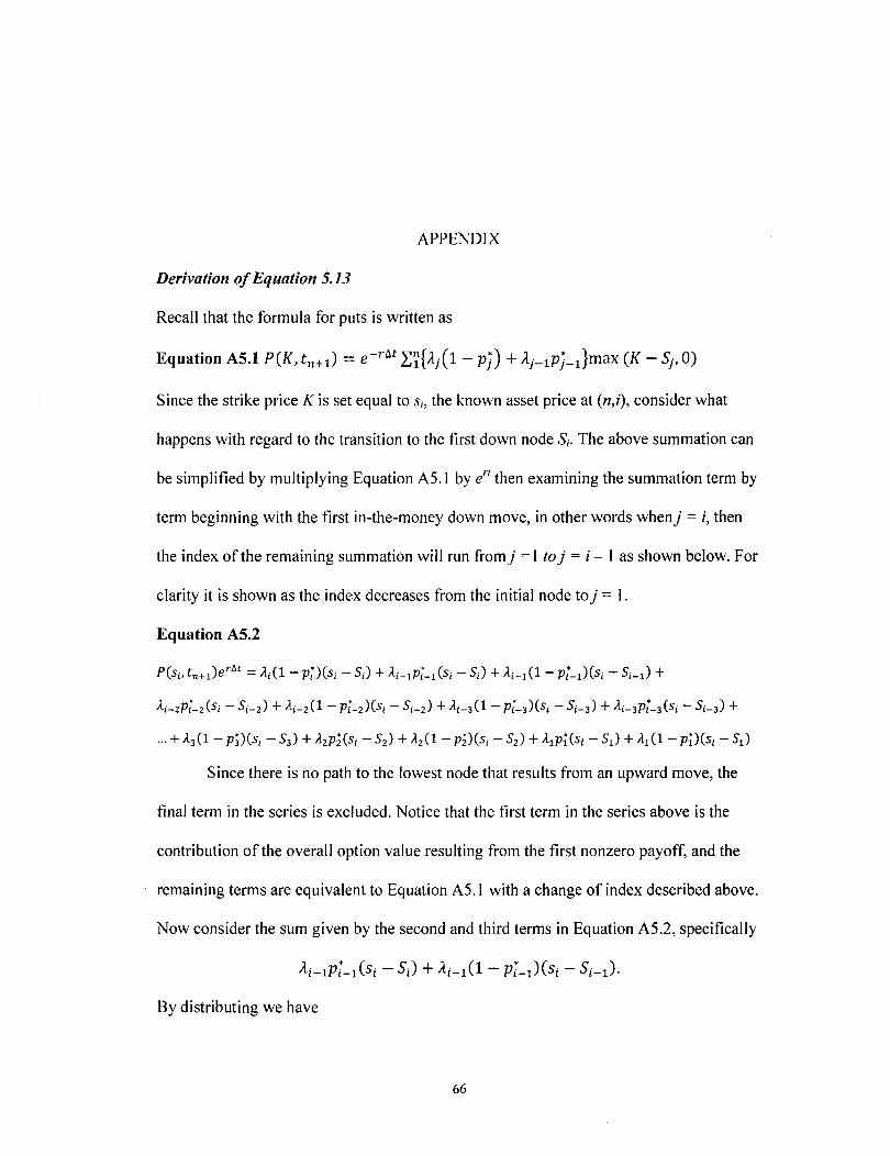
APPENDIX

Derivation of Equation 5.13

Recall that the formula for puts is written as

Equation AS.1 P(K, tn +1) == e-rllt LNAll - pj) + Aj_lPj_l}max (K - Sj' 0)

Since the strike price K is set equal to Sj, the known asset price at (n,i), consider what

happens with regard to the transition to the first down node Sj. The above summation can

be simplified by multiplying Equation AS.1 by err then examining the summation term by

term beginning with the first in-the-money down move, in other words when} = i, then

the index of the remaining summation will run from} =1 to} = i-I as shown below. For

clarity it is shown as the index decreases from the initial node to} = 1.

Equation AS.2

pes;, tn+ l )eTtlt = ,1;(1 - pi)(s; - 5a + AHPi-l (s; - 5a + ,1;-1 (1 - Pi-l)(S; - 5;-1) +

A;_2P;'_2(s; - 5i - 2) + ,1;-2(1 - P;'-2)(Si - 5;-2) + ,1;-3(1- P;'-3)(Si - 5;-3) + A;-3P;'-3(Si - 5;-3) +

... + ,13(1- p3)(s; - 53) + A2Pi(s; - 52) + ,12(1 - pD(s, - 52) + AIP;(S; - 51) + ,11 (1- P;)(Si - 51)

Since there is no path to the lowest node that results from an upward move, the

final term in the series is excluded. Notice that the first term in the series above is the

contribution of the overall option value resulting from the first nonzero payoff, and the

remaining terms are equivalent to Equation AS.1 with a change of index described above.

Now consider the sum given by the second and third terms in Equation AS.2, specifically

Ai-1Pt-l (Si - Si) + Ai-l (1 - Pt-l)(Si - Si-l)'

By distributing we have

66

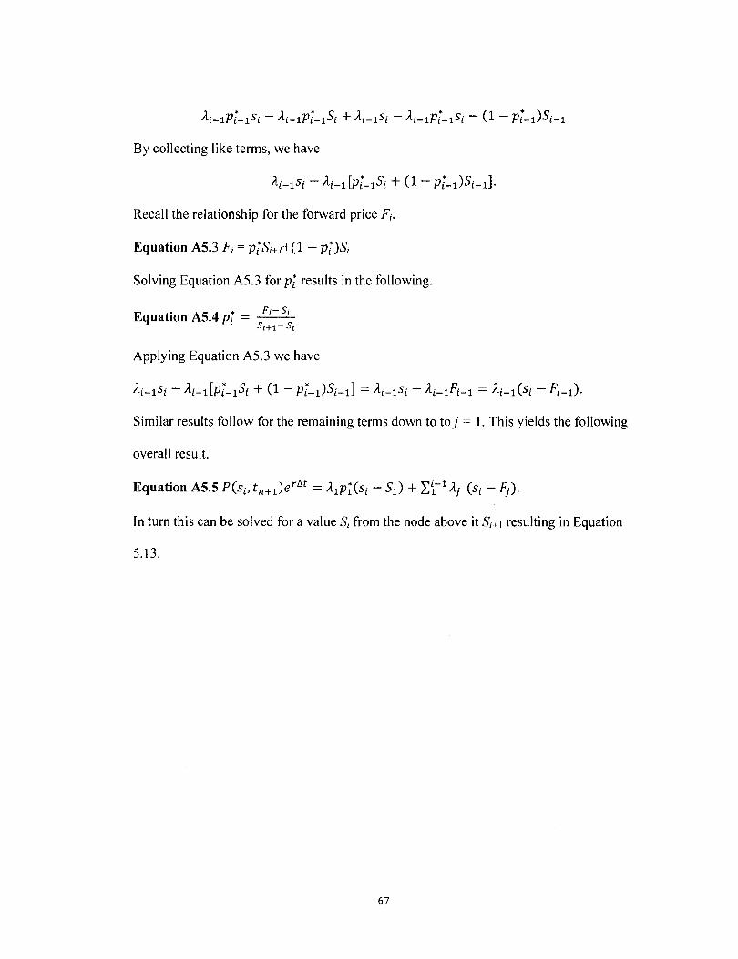
By collecting like terms, we have

Recall the relationship for the forward price Fi .

Equation AS.3 Fi = PiSi+l+(l - Pi)Si

Solving Equation A5.3 for pi results in the following.

p·-s· Equation AS.4 pi = ! !

Si+I-Si

Applying Equation A5.3 we have

Similar results follow for the remaining terms down to to j = 1. This yields the following

overall result.

In turn this can be solved for a value Si from the node above it Si+1 resulting in Equation

5.13.

67

NAME:

ADDRESS:

DOB:

EDUCATION & TRAINING:

CURRICULUM VITAE

Brian Butler

2200 Cross Hill Rd Louisville, KY 40206

Louisville, KY - October 18, 1969

B.A., Mathematics Humboldt State University 1989-1993

Exam liP, Probability Society of Actuaries 2002

Exam FM, Financial Mathematics Society of Actuaries 2006

Validation by Educational Experience, Corporate Finance Society of Actuaries 2007

Validation by Educational Experience, Economics Society of Actuaries 2007

Validation by Educational Experience, Applied Statistics Society of Actuaries 2007

Minisymposium on Financial Mathematics Purdue University April 2005

68