University of Louisville University of Louisville

ThinkIR: The University of Louisville's Institutional Repository ThinkIR: The University of Louisville's Institutional Repository

Electronic Theses and Dissertations

8-2013

The GC3 framework : grid density based clustering for The GC3 framework : grid density based clustering for

classification of streaming data with concept drift. classification of streaming data with concept drift.

Tegjyot Singh Sethi University of Louisville

Follow this and additional works at: https://ir.library.louisville.edu/etd

Recommended Citation Recommended Citation Sethi, Tegjyot Singh, "The GC3 framework : grid density based clustering for classification of streaming data with concept drift." (2013). Electronic Theses and Dissertations. Paper 1300. https://doi.org/10.18297/etd/1300

This Master's Thesis is brought to you for free and open access by ThinkIR: The University of Louisville's Institutional Repository. It has been accepted for inclusion in Electronic Theses and Dissertations by an authorized administrator of ThinkIR: The University of Louisville's Institutional Repository. This title appears here courtesy of the author, who has retained all other copyrights. For more information, please contact thinkir@louisville.edu.

THE GC3 FRAMEWORK

GRID DENSITY BASED CLUSTERING FOR CLASSIFICATION OF STREAMING

DATA WITH CONCEPT DRIFT

By

Tegjyot Singh Sethi

B.Tech., GITAM University Visakhapatnam, 2012

A Thesis

Submitted to the Faculty of the

J.B. Speed School of Engineering of the University of Louisville

in Partial Fulfillment of the Requirements

for the Degree of

Master of Science

Department of Computer Engineering and Computer Science

University of Louisville

Louisville, Kentucky

August 2013

ii

THE GC3 FRAMEWORK

GRID DENSITY BASED CLUSTERING FOR CLASSIFICATION OF STREAMING

DATA WITH CONCEPT DRIFT

By

Tegjyot Singh Sethi

B.Tech., GITAM University, Visakhapatnam, 2012

A Thesis Approved on

July 24, 2013

By the following Thesis Committee:

____________________________________

Dr. Mehmed Kantardzic, CECS (Thesis Director)

____________________________________

Dr. Adel S. Elmaghraby, CECS

____________________________________

Dr. Gail W. DePuy, IE

iii

DEDICATION

This thesis is dedicated to my parents

Mr. Man Mohan Singh Sethi

and

Mrs. Gurinder Kaur Sethi

who have always loved and supported me.

iv

ACKNOWLEDGEMENTS

The author would like to thank his advisor Dr. Mehmed Kantardzic for all his

support, and guidance. This thesis would not have been possible without his continued

encouragement and advice. The author would also like to convey his sincere appreciation

to the members of his thesis committee: Dr. Adel S. Elmaghraby and Dr. Gail W. DePuy,

for their valuable suggestions and patience. The author would like to thank Dr. Olfa

Nasraoui for her advice and insight in this field. The author would like to thank his

family back in India for their support and encouragement to pursue a graduate education.

The author also thanks the members of his family in Chicago, Illinois, Devinder and

Rachita Singh, for their continued motivation. Finally, special thanks are extended to

Angad, Ankita and Jia for their unconditional love and trust.

v

ABSTRACT

THE GC3 FRAMEWORK

GRID DENSITY BASED CLUSTERING FOR CLASSIFICATION OF STREAMING

DATA WITH CONCEPT DRIFT

Tegjyot Singh Sethi

July 24, 2013

Data mining is the process of discovering patterns in large sets of data. In recent

years there has been a paradigm shift in how the data is viewed. Instead of considering

the data as static and available in databases, data is now regarded as a stream as it

continuously flows into the system. One of the challenges posed by the stream is its

dynamic nature, which leads to a phenomenon known as Concept Drift. This causes a

need for stream mining algorithms which are adaptive incremental learners capable of

evolving and adjusting to the changes in the stream.

Several models have been developed to deal with Concept Drift. These systems

are discussed in this thesis and a new system, the GC3 framework is proposed. The GC3

framework leverages the advantages of the Gris Density based Clustering and the

Ensemble based classifiers for streaming data, to be able to detect the cause of the drift

and deal with it accordingly. In order to demonstrate the functionality and performance of

the framework a synthetic data stream called the TJSS stream is developed, which

embodies a variety of drift scenarios, and the model’s behavior is analyzed over time.

vi

Experimental evaluation with the synthetic stream and two real world datasets

demonstrated high prediction capability of the proposed system with a small ensemble

size and labeling ratio. Comparison of the methodology with a traditional static model

with no drifts detection capability and with existing ensemble techniques for stream

classification, showed promising results. Also, the analysis of data structures maintained

by the framework provided interpretability into the dynamics of the drift over time. The

experimentation analysis of the GC3 framework shows it to be promising for use in

dynamic drifting environments where concepts can be incrementally learned in the

presence of only partially labeled data.

vii

TABLE OF CONTENTS

PAGE

ACKNOWLEDGEMENTS ...................................................................................................iv

ABSTRACT ..................................................................................................................v

TABLE OF CONTENTS .......................................................................................................vii

LIST OF TABLES .................................................................................................................ix

LIST OF FIGURES ...............................................................................................................xi

INTRODUCTION .................................................................................................................1

1.1 Stream data mining and its challenges .............................................................1

1.2 Formal Problem Statement: Classification of Streaming Data ........................3

1.3 Introduction to the GC3 Framework ................................................................4

1.4 Goals ................................................................................................................5

1.5 Organization of the Thesis ...............................................................................6

REVIEW OF CONCEPT DRIFT IN LITERATURE ..........................................................7

2.1 Concept Drift ...................................................................................................7

2.2 Existing systems for dealing with Concept Drift .............................................11

2.3 Ensemble of Classifiers for Streaming Data ....................................................14

2.4 Classification upon Clustering for Streaming Data .........................................18

2.5 Stream Clustering Algorithms .........................................................................23

PROPOSED METHODOLOGY: THE GC3 FRAMEWORK..............................................29

viii

3.1 Introduction ......................................................................................................29

3.2 Overview of the GC3 Framework....................................................................30

3.3 Notation and Basic Definitions for the GC3 Framework ................................33

3.4 Data Structures Maintained in the GC3 Framework ........................................36

3.5 Components of the GC3 Framework ...............................................................41

3.6 Parameters of the GC3 Framework ..................................................................59

EXPERIMENTAL EVALUATION WITH THE SYNTHETIC DATA STREAM .............69

4.1 Description of the Synthetic Data: The TJSS Stream ......................................69

4.2 Experimentation and Analysis on the TJSS stream .........................................74

4.3 Comparison of GC3 Framework with a Traditional Static Model ..................88

4.4 Robustness of the Dynamic Grid Clustering ...................................................91

EXPERIMENTAL EVALUATION WITH REAL WORLD DATASETS ..........................93

5.1 Description of the Datasets ..............................................................................93

5.2 Experimentation and Analysis .........................................................................97

5.3 Comparison of the GC3 Framework with Existing Techniques ......................110

5.4 Why the GC3 Framework performs better than SVE, WE and Woo

methodology? ...................................................................................................117

CONCLUSION AND FUTURE WORK ..............................................................................120

REFERENCES ..................................................................................................................123

APPENDICES ..................................................................................................................128

CURRICULUM VITAE ........................................................................................................136

ix

LIST OF TABLES

TABLE PAGE

1. Categorization of Parameters: Data Dependent Parameters and Data Independent

Parameters. .................................................................................................................. 61

2. User Specified Parameters.(TJSS Stream) .................................................................. 75

3. Estimated Threshold Values. (TJSS Stream) .............................................................. 75

4. Performance Measures.(TJSS Stream) ....................................................................... 76

5. Accuracy Measures for at (τ,nb).( TJSS Stream) ........................................................ 85

6. Number of New Models Generated at (τ,nb).(TJSS Stream) ...................................... 85

7. Area Under ROC Curve Measures at (τ,nb).( TJSS Stream) ...................................... 86

8. User Specified parameter values for Comparison with static classifiers. ................... 88

9. Comparison of Performance of GC3 Framework and Traditional Models on the TJSS

stream. ......................................................................................................................... 89

10. User Specified parameters for experimentation with Real World datasets. ............... 97

11. Threshold values estimated from pre experimentation.(MAGIC dataset) .................. 98

12. Performance measures on the MAGIC dataset. .......................................................... 98

13. Accuracy Measures for Different values of τ and nb.(MAGIC dataset) ................... 101

14. Number of New Models Generated.(MAGIC dataset) ............................................. 102

15. Area Under ROC Curve Measures.(MAGIC dataset) .............................................. 102

x

16. Threshold values estimated from pre experimentation.(EM dataset) ....................... 103

17. Performance measures on the EM dataset. ............................................................... 104

18. Accuracy Measures at (τ, nb).(EM dataset) ............................................................... 107

19. Number of New Models Generated at (τ, nb)(EM dataset). ...................................... 108

20. Area Under ROC Curve Measures at (τ, nb) (EM dataset). ...................................... 108

21. Confidence Interval on the Performance Measures.(EM dataset) ............................ 109

22. User Specified parameter values for Comparison of GC3 Framework. ................... 110

23. Comparison of Performance of Traditional Model and the GC3 Framework (Real

World Ddatasets). ..................................................................................................... 112

24. Comparison with Nom, λ and WSF on SVE, WE and Woo ensemble. ................... 115

25. User Specified Parameter Values (TJSS Stream) ..................................................... 133

26. Intermediate Results from pre experiment. ............................................................... 133

27. Final Threshold values (TJSS Stream) ..................................................................... 134

28. User Specified Parameter Values(MAGIC Dataset) ................................................. 134

29. Intermediate Results from pre experiment(MAGIC Dataset) ................................... 134

30. Final Threshold values (MAGIC Dataset) ................................................................ 134

31. User specified parameter values (EM dataset).......................................................... 135

32. Intermediate Results from pre experiment (EM dataset). ......................................... 135

33. Final Threshold values (EM dataset). ....................................................................... 135

xi

LIST OF FIGURES

FIGURE PAGE

1. Causes of Concept Drift: Data Distribution drift and Class Distribution drift. ...... 9

2. Types of Concept Drift. ........................................................................................ 11

3. Ensemble of classifiers for streaming data. .......................................................... 15

4. Generation of new classifiers based on misclassified sample points .................... 20

5. The D-Stream Clustering ...................................................................................... 26

6. The GC3 Framework. ........................................................................................... 30

7. Combining clusters by modifying the Cluster_tree. ............................................. 39

8. Algorithm: Grid Density Clustering. ................................................................... 43

9. Cluster Dynamics. Merger, Extension and Creation of Clusters .......................... 46

10. Classifying new sample using two step weighted aggregation. ............................ 50

11. Algorithm: Update Cluster Ensemble. .................................................................. 58

12. Adjust Ensemble Workflow. ................................................................................. 59

13. Procedure: Pre experimentation for estimating parameter value ......................... 66

14. Progression of the TJSS stream.(a-j) .................................................................... 72

15. Component Clusters of the TJSS stream. ............................................................. 73

16. ROC Curve for Initial Experiment on TJSS stream.............................................. 76

xii

17. Accuracy over time. (TJSS Stream)...................................................................... 77

18. Recovery Points in the stream’s progression. (TJSS Stream)............................... 78

19. Cluster_tree depicting hierarchies of cluster at the end of the TJSS Stream. ....... 81

20. Accuracy at (τ,nb) (TJSS Stream). ........................................................................ 86

21. Accuracy and Number of Models at (τ,nb) (TJSS Stream). .................................. 87

22. Comparison of Accuracy over time for GC3 framework and Traditional Static

Models on the TJSS Stream. ................................................................................. 89

23. Comparison of Performance on TJSS stream. ...................................................... 90

24. TJSS stream with 25% salt and pepper noise added. ............................................ 91

25. Clusters predicted by GC3 framework on the Noisy TJSS stream. ...................... 92

26. Accuracy over time. (MAGIC dataset). ................................................................ 99

27. Cluster_tree obtained at end of the MAGIC dataset stream. .............................. 100

28. Accuracy, Recovery Points, list of models generated over time on the EM dataset.

............................................................................................................................. 105

29. Cluster_tree at the end of the EM dataset. .......................................................... 106

30. Probability plot illustrating normality of Nom and accuracy values obtained on

the EM stream. .................................................................................................... 109

31. Comparison of Accuracy over time (MAGIC dataset). ...................................... 111

32. Comparison of Accuracy over time (EM dataset). ............................................. 111

33. Comparison of performance with Traditional model. (MAGIC dataset). .......... 112

34. Comparison of performance with Traditional model. (EM dataset). .................. 113

35. Comparison of WSF, Nom and λ for GC3 framework, SVE, WE and Woo

ensemble. ............................................................................................................ 116

xiii

36. Components of the TJSS stream ......................................................................... 128

37. Evolution of Cluster A(TJSS Stream)................................................................. 129

38. Evolution of Cluster B(TJSS Stream). ................................................................ 130

39. Evolution of Cluster C (TJSS Stream). ............................................................... 130

40. Evolution of Cluster D(TJSS Stream)................................................................. 132

41. Evolution of Cluster E(TJSS Stream). ................................................................ 132

1

CHAPTER 1

INTRODUCTION

1.1 Stream data mining and its challenges

A data stream refers to a continuous flow of ordered data records in and out of a

system [1]. With the growth in sensor technology and the big data revolution, large

quantities of data are continuously being generated at a rapid rate. Whether it is from

sensors installed for traffic control or systems to control industrial processes, data from

credit card transactions to network intrusion data, streaming data is ubiquitous. Today

almost all forms of data being collected is streaming as we do not stop collecting data to

make analysis on it, but instead the analysis and the data collection happens

simultaneously. This poses a major challenge with the timeliness of the prediction results.

The analysis results from historical data would fail to account for the current state of the

system and as such will not be totally reliable. Also the rate at which this data is being

generated (real time in many cases) is much higher than the rate at which it can be

analyzed by traditional data mining techniques.

In such a dynamic environment, the basic tasks of Data mining such as Clustering,

Classification, Summarization, etc. are no longer trivial. There is a paradigm shift from

the traditional techniques where the system is presented with all the historical data and a

model is built on it, using if needed a validation set, and this model once built is used

without change for all future predictions. Such a static model does not fit well in the real

2

world scenario as the data encountered in most cases is itself dynamic and embodies

constant changes in the environment. Also, the huge amount of data flowing into the

system poses practical restrictions on the memory and the amount of data that can be

stored and processed at each time interval. Thus the algorithms for stream mining need to

be more selective as to what data they store and what they disregard.

All these concerns have led to a lot of research in the recent years to overcome these

challenges posed by streaming data. The main characteristics of streaming data that need

to be addressed by any model developed was described in [1,2] and is summarized below.

Scalability and Response Time: As the data stream may, in principle, be an

infinite source of data, it is not possible to store all the data for performing the

analysis. Thus the model needs to analyze data in chunks and store only a very

small portion of this data in the main memory. Also, since the data is

continuously pouring in, the response needs to be in near real time in most cases,

for it to be of any practical use.

Robustness: Any real world process is bound to exhibit noise and distortions in

the data being generated. A system needs to be robust to these factors and work

even in the presence of such changes. This problem is even more challenging in

case of streaming data, as the data is dynamic and it is necessary to distinguish

the noise from the changes in the environment. The model needs to balance

between being overly sensitive to noise and at the same time being able to detect

changes and learning from them.

Concept Drift: The major challenge with streaming data is that of adaptability.

The distribution generating the data might change over time and the model

3

generated needs to detect and adjust to such changes automatically. This is what

makes mining of streaming data different from traditional mining techniques.

This change in the generating model with the passage of time is known as

Concept Drift.

In this thesis the challenge posed by Concept Drift is considered. The GC3

incremental learning framework is proposed to detect and adapt to changes in an evolving

data stream.

1.2 Formal Problem Statement: Classification of Streaming Data

The data mining task considered here is: Classification. A stream of data is

evaluated one at a time and the class label associated with each sample is estimated. A

good model would provide high estimation capability within the limitations of time and

memory resources.

Consider a stream of samples represented by X1, X2,…XInf ; where Xi is a vector

representing an input sample. Each Xi has an associated Yk which is its class label.

Furthermore consider the value initial_train_stream, For all Xj, j< initial_train_stream,

the corresponding Yk are available. For Xj , j> initial_train_stream, only a few of the Yk’s

are available. The task is to predict these Yk’s given only the prior information about the

samples. Probabilistically the task of classification is the probability that the class label is

Yk given the sample is Xi denoted by the conditional probability p(Yk| Xi).

When dealing with static data, the common assumption is that the probability

distribution of the data does not change with time. i.e. pt(Y| Xi) =pt+1(Y| Xi). However, in

case of streaming data with concept drift, this assumption is not valid as the distribution

4

of data and their corresponding probabilities change with time. Classifying data in

streams involves a continuous incremental learning framework which is capable of

receiving feedback and evolving from the changes, if any.

1.3 Introduction to the GC3 Framework

The GC3 Framework: Grid density based Clustering for Classification of streaming

data with Concept drift, is proposed in this thesis, as a new approach to classify data that

is dynamically changing. It is an incremental learning framework which is capable of

detecting and handling Concept Drift in streaming data. It is based on the idea of

‘Clustering upon Classification’, which builds classifiers on top of clusters to incorporate

the advantages of both methodologies. The GC3 Framework augments the effectiveness

of Ensemble Classifiers by combing them with clustering and grid density representation.

Here, the entire input space is divided into grids and dealt in discrete blocks to make the

computations less expensive and provide robustness. The GC3 framework maintains

ensembles at two levels, the Global Ensemble made up all the models in the system and

the Cluster Ensemble which comprises of models maintained by a particular cluster

locally, to deal with the drifts according to the nature of their occurrence. A novel

aggregation procedure is proposed which combines the ensemble outputs considering

both its Similarity to a distribution and it’s Recentness in time. A synthetic stream called

the TJSS stream is developed which demonstrates various scenarios that could occur in a

drifting environment, and in subsequent experimental analysis it is found that the GC3

framework is able to deal with all of them effectively. Also, experimentation with two

5

real world streams demonstrates the applicability of the GC3 framework for practical real

world applications.

1.4 Goals

The goal of this thesis is to study prior solutions and propose a new model for the

classification of streaming data with concept drift. The new model proposed needs to be

described in detail to demonstrate its functionality, the reason for choosing each of its

components and their relevance to the task at hand. The novelty of the work presented

here would be in developing a new framework capable of dealing with concept drift, with

comparatively better performance and interpretation ability than existing systems. It is

therefore necessary to evaluate and to analyze how the methodology compares to existing

techniques used to handle concept drift. Also, necessary is the evaluation of the model on

standard real world datasets to demonstrate its applicability to real word streams.

For the purpose of illustrating the functionality of the proposed methodology, a

synthetic stream is developed which encompasses various types of drifts and can be used

by other grid density algorithms to see how they handle these scenarios that could occur

in a dynamic environment.

Finally, as every parametric model needs the parameters to be tuned so as to give

optimal performance; a methodology is required to derive the values for these parameters

from analysis of the data being used.

6

1.5 Organization of the Thesis

Chapter 2 introduces Concept Drift formally and describes the various types and

causes of drift. It also provides a brief overview of the existing techniques developed to

deal with concept drift. The ensemble classification techniques proposed by Woo et al. in

[32, 33, 34] and the grid density clustering described in [35,36] lay the foundation for the

development of the GC3 framework. Chapter 3 introduces the GC3 framework and

provides detailed explanation of its various components and their working. Important

notation and definitions are also presented in this chapter, along with a subsection on how

the parameters of the system can be specified for any type of data based on pre

experimentation. The TJSS synthetic data stream is described and experiments on it are

presented in Chapter 4. In Chapter 5 experiments with two real world datasets, the

MAGIC and the Electricity Market datasets are presented along with a detailed analysis

of the results. Chapter 6 gives the concluding remarks and the scope for future work in

this area.

7

CHAPTER 2

REVIEW OF CONCEPT DRIFT IN LITERATURE

In this chapter, the idea of Concept Drift is formally introduced and existing

techniques which have been developed to deal with it are presented. Section 2.1 presents

the types of concept drift and the causes for drift. Existing methodologies to deal with

concept drift are presented in Section 2.2 and 2.3. In Section 2.4, the idea of

‘Classification upon Clustering’ is introduced which lays the foundation for the GC3

framework. The present state of the art in grid density clustering is presented in Section

2.5 which will be extended in Chapter 3 to make it a part of the GC3 framework.

2.1 Concept Drift

The data arriving in real world streams is constantly evolving over time. The model

as well as the underlying distribution of the data could change, making the generated

model obsolete and no longer usable. This phenomenon is known as Concept Drift.

Consider, for example, a customer profiling model which learns customer preferences

based on their purchase history. Furthermore, consider a customer just out of college and

starting a full time job. The preference model for such a customer would drift as the

customer now has more buying potential and the existing model of his spending is no

longer valid. Thus there is a need for a model that can adapt and learn incrementally from

8

such changes in its environment. The following sections discuss the causes of concept

drift from a probabilistic perspective and then lists out the various types of drifts based on

their occurrence patterns.

2.1.1 Causes of Concept Drift

The change in the distribution of streaming data is known as Concept Drift. The

classification of streams can be viewed as a joint probability distribution model as

depicted below [3] [4].

P(xi,yj)=P(xi). P(yj|xi) ; xi ϵX, yj ϵY (x) (2.1)

Here, X denotes the set of feature vectors and Y denotes the set of classes. The

stream could be seen as an infinite sequence of (xi,yj). In this case the possible sources of

drift could either be a change in the value of P(x), known as Dataset Distribution Drift, or

a change in the value of P(y|x), known as the Class Distribution Drift, or both.

a) Dataset Distribution Drift: A drift in the distribution of feature vectors could

affect the classification process of streams. Such a drift could occur if previously

unseen features become more prominent or the entire data starts moving to a

different part of the feature space. Such a drift could occur independent of any

change in class distribution and is possible even in the absence of any change in

the model. In such a case this type of drift is also referred to as virtual drift. These

changes can cause the performance of the learned model to degrade, even if the

underlying concept did not change. Thus it is useful to have an adaptive model to

learn from such data. This type of concept drift is essential in case of imbalanced

data, when previously unseen feature vectors appear over time.

9

b) Class Distribution Drift: This is also referred to as real drift and it occurs due to a

change in the posterior probabilities of class memberships P(y|x). This is the most

common kind of drift addressed in research and the streaming data mining

methodologies developed. This represents a change in the model boundary and

hence there is a need to update the classifier accordingly.

Concept drift in the data could occur due to either of the above mentioned reasons

and in most real world applications, a combination of both is observed. From a practical

point of view both the real and virtual drift could be considered equivalent as they both

ultimately lead to changes in P(x,y). The Figure 2.1depicts changes in concepts at time t1

and t2, where t1<t2.

Figure 2.1: Causes of Concept Drift: Data Distribution drift and Class Distribution drift.

In Figure 2.1, the causes of drifts are depicted. ‘Concept a’ depicts a model change

where the class boundary changes even though the distribution remains constant.

‘Concept b’ undergoes both a distribution and a model drift. ‘Concept c’ initially is not in

the system, it is however present at time t2, demonstrating a case of purely data

10

distribution drift. All these changes embody the Concept drift that causes the data to

change from time t1 to t2.

2.1.2 Types of Concept Drift

In the previous section, the causes for concept drift were addressed from a

probabilistic perspective. Here, the various types of concept drifts, based on the speed

and patterns of drift, are listed [5][6].

a) Sudden Drift: This is the simplest form of concept drift to detect and deal with. It

occurs when at a particular time td, the generating function f0 is replaced with

another function f1. An example of such a drift could be implementation of a new

tax policy and the effect on the financial market following it.

b) Incremental Drift: In this type of drift it is often difficult to draw a clear boundary

between the occurrences of the two generating function and it encompasses a

fuzzy region which shows gradual changeover to the new concepts. For example

the performance of a player in any sport could be seen as an incrementally

improving concept.

c) Reoccurring Drift: This is a class of drift in which previously active concepts

recur over a period of time. The periodic occurrence is however not fixed and can

be observed at random intervals. This is seen when we look at the sales of any

popular band’s merchandise which tends to go up usually about the time a new

album is released.

Figure 2.2 depicts the above mentioned types of drifts. The plots are against the time axis

and the different colored spots represent different concepts. The similar colored spots all

represent the same concept.

11

Figure 2.2. Types of Concept Drift.

2.2 Existing systems for dealing with Concept Drift

Irrespective of the type of drift that may occur, the main components of any system

designed to deal with drift are as given below:

A Drift Detection component that notifies that a drift has occurred, and

A Drift Adaptation component that adjusts learning based on the drift.

In recent years a lot of research has been undertaken in this area and various

techniques have been developed to be used with dynamic streams. These are classified as

given below.

a) Incremental adaptive base learning algorithms:

This technique involves developing base learners that can adapt to changes in

the data and evolve over time. Several such algorithms have been developed

12

which modify the well-known traditional data mining algorithms into

adaptive learners.

Decision trees are one of the well-known and studied classification

methodologies of all time. The C4.5 algorithm is widely used implementation

of Decision trees [7]. Based on the C4.5 algorithm an extension for streaming

data was proposed in [8], called Very Fast Decision Tree (VFDT), which

uses Hoeffding bounds [9] to grow decision trees in streaming data.

Hoeffding bounds provide a way to develop confidence intervals around the

mean of a distribution. Several variants of the VFDT have been proposed.

The Concept-adapting Very Fast Decision Trees (CVFDT) described in

[11,13] uses a sliding window of instances which are used to generate and

update statistics at each node. The Hoeffding Window Tree (HWT) and the

Hoeffding Adaptive trees (HAT) are also extensions of the decision trees

which employ the concept of a sliding window of instances to update the

model [10]. HAT employs an adaptive window size and hence is more

efficient. Further extension to these models led to the development of

Hoeffding Options Trees (HOT) where a node can be regarded as an option

node which splits the path of the tree along multiple nodes [12].

Other extensions to basic algorithms to deal with streaming data have

been proposed in literature. Adaptive kNN proposed in [15] demonstrates the

use of the K Nearest Neighbor classifier for streaming data, in case when

either there is a drift or the data is stable. In [14] a streaming model for

Support Vector Machines is developed by leveraging connections between

13

learning and computational geometry, to produce a one pass SVM model on

streams.

b) Dataset Adaptive Models:

In these techniques, changes are made to the training dataset to make it

usable with a classifier. Instance Weighting and Selection are common

approaches.

In Instance Selection, a sliding window is employed select instances

relevant to the current concept. The window size in this case could be a

parameter which is fixed as in FLORA, or it could be adaptive and could vary

based on heuristics over the data as in FLORA2 [16, 17]. In [18], use of

multiple windows was proposed. The two windows had different sizes, with

the smaller one being updated constantly based on arrival of data, while the

larger one is updated upon detection of concept drift.

In the case of Instance Weighting, the instances are given relative

importance. They then depend on algorithms that can learn these weights.

SVMs were used in [19] to process weighted instances.

c) Ensemble Classifiers:

One of the most widely used techniques for dealing with streaming data is the

use of an Ensemble of Classifiers for modeling the stream [21-34]. The basic

principle of ensemble classifiers is that of combining several weak and

independent classifiers to produce a strong model on the entire data. The

ensemble technique has proven to be empirically effective and is used in

place of traditional one model fits all techniques. Ensemble Classifiers are

14

particularly advantageous for stream classification, owing to the fact that new

models can be added to the ensemble as the concept evolves. In case of

Reoccurring Drifts, models trained over previous concepts could be used and

their weight could be increased to show that they are once again prevalent.

Also, Ensemble Classifiers leverage already established base learning

algorithms to work with streams. The Ensemble Classifiers have become the

De facto classifiers for streams in recent years. The various types of ensemble

techniques that can be used with streams are discussed in the next section.

2.3 Ensemble of Classifiers for Streaming Data

Ensemble Classifiers have gained a lot of popularity owing to their empirical

effectiveness. This effectiveness stems from the principle of ‘Wisdom of the crowd’,

which states that the collective decision taken by the group is often more effective than

decision taken by any individual in the group independently [54]. In accordance with this

principle, ensemble classifiers provide outputs combined from a set of independent

models trained on different parts of the data (leading to weak models), and in doing so

they result in high accuracy and robustness in the final decision. Traditional ensemble

methods such as Bagging, Boosting, Stacking and random forests [20-22] have found to

be effective for various classification problems.

In the world of streaming data, ensemble methods are the most popular and widely

studied techniques to handle concept drift and the evolving nature of the stream. The

basic structure of an ensemble classifier as used to mine streams is shown in the Figure

2.3.

15

Figure 2.3: Ensemble of classifiers for streaming data.

As is depicted in Figure 2.3, the incoming data is either split into chunks or dealt

incrementally one sample at a time. In the training phase, the input data is mapped to

various groups and a separate model is trained on each of these datasets. These models

are entered into the ensemble set and together they form the trained ensemble

16

classifier. When given an unlabeled sample to make a prediction on, the models in the

ensemble come up with their individual solutions and a combining strategy is then used

to give the final output. Based on how the ensemble set is maintained and the combining

strategy is implemented the ensemble methodologies can be grouped as described in [23]

and given below:

a) Dynamic Combiners (horse-racing): In this method, individual models making up

the ensemble are trained and the forgetting process is modeled by changing the

combining strategy of the outputs. Here, the individual models are trained in

advance and are not retrained at any further stage. The Weighted Majority

algorithm is an example of such a type of classifier [24]. The disadvantage of

such a model is that over time the performance of all the experts might degrade

and then any change to the combination rules might not be effective in

maintaining the performance of the ensemble.

b) Updated Training data: In this type of ensembles, the incoming data creates

models incrementally. The specific technique used to build and combine these

models leads to its various variants. The Streaming Ensemble Algorithm

described in [25] has a window which captures the incoming data and then uses

chunks of data to create a new model which is added to the ensemble set. If this

set is full, then the least performing model is pruned. In [26] an online bagging

algorithm is proposed in which the experts are trained incrementally and a

decision is made based on a majority voting scheme.

c) Changing the Ensemble structure: Changing the ensemble structure, involves

adding or deleting models from the set based on the most recently arriving

17

data. Performance of this category of ensembles depends on the method of

pruning used, the number and timeliness of the new classifiers spawned and the

old ones dropped. The Dynamic Weighted Majority (DWM) [27, 28] is an

incremental technique which maintains the overall classification performance by

dynamically increasing or decreasing the ensemble set size. Weighted Ensembles

proposed in Wang et al [29], use the current data chunk as the testing dataset and

eliminates those classifiers in the ensemble whose performance on the e chunk

was less than a threshold.

d) Updating the ensemble members: Here the members of the ensemble are retrained

based on the new data arriving. The least performing member is retrained on the

current data chunk. The Adaptive Ensemble Classifier (ACE) proposed in [30]

has three components, the Online component which is any incremental learner

that gets trained on every new sample, the Batch component that maintains long

term memory for retraining the model in case of a drift, and a Drift detection

mechanism. ACE updates the ensemble members and also the combination rules

based on the new data arriving.

e) Adding New features: As the importance of features evolves, the attributes used

by models in the set are changed without retraining the entire ensemble.

The above described methodologies barely scratch the surface of the entire work that

has been done in the field of ensemble learning for streaming data. One other category

which has proven to be effective is described below:

f) Classification upon Clustering: In this methodology, the incoming data is

clustered using a stream clustering algorithm, and then a separate classifier is

18

trained on each of these clusters to generate the set of ensembles. The advantage

of these methods is that it differentially captures both the major cause of drift: the

drift in the data distribution and that in the classifier boundary. The following

section elaborates upon this idea and also discusses work done in this area as

related to streaming data mining.

2.4 Classification upon Clustering for Streaming Data

An interesting approach to classifying streaming data was proposed in [31]. In this

paper, a Conceptual Clustering and Prediction (CCP) framework was proposed. The CCP

framework uses incremental clustering to group similar concept together and then trains

models on individual concepts to form an ensemble set. The main components of this

system are: A Mapping Function to transform data to a probabilistic representation, an

Incremental Clustering algorithm to group incoming vectors based on similarity and an

Incremental Classifier to make the predictions.

This approach to handling concept drift is theoretically effective because the

clustering component handles the drift caused by change in the distribution of data or

P(x) and the classification handles the change in the model or P(y|x), as described in

Section 2.1 . In [32], Woo et al developed an ensemble approach to classifying streaming

data based on misclassified sample points. In this paper and in the following work in [33]

and [34], they have demonstrated the effectiveness of their algorithm which is based on

clustering and subsequent classification of streaming data.

19

2.4.1 Ensemble Classifier based on Misclassified Streaming Data

This method is due to Woo et al [32-34]. In this approach, an ensemble maintains a

set of models, each native to a particular region in the multidimensional feature space. If

a new sample needs to be classified, it is mapped to its corresponding cluster and the

model associated with that particular cluster is used to make predictions on that sample. It

is postulated that such samples have high probability of being correctly classified as they

use the model local to their spatial location. If a new sample point occurs in a region

where there is no previously defined model, then such a sample is termed as a

‘Suspicious Sample’. When a ‘Suspicious Sample’ is detected, weights to this unlabeled

sample from each of the classifiers in the current ensemble set are evaluated and a

weighted majority voting is carried out to predict its label. These suspicious samples are

also regarded as potential seeds for new clusters as the data evolves. The process of

generating and classifying the samples as proposed by Woo et al is described below.

2.4.1.1 Generating a new classifier

In this method, each classifier is associated to a cluster. These clusters are spherical

and have an associated density and radius given by θs and θr respectively. The centroid of

the cluster is given by the mean of all the samples in the cluster is called the

‘Representative Candidate’ (RC), which is used further in Similarity calculations for

classifying new unlabeled data. Initially, a new model is generated on all the training set,

and added to the ensemble. In the streaming phase, any new sample which falls outside

the boundary is termed as a ‘Suspicious Sample’ and it is used to define a new cluster

region. When subsequent samples are clustered to this new region, the seed is not moved

until a predefined threshold density θs is reached. Once the number of sample points in

20

this cluster reaches this density threshold, this cluster is removed from the ensemble and

a classifier is trained on this by asking for the necessary percentage of labeled data. The

RC is recomputed on this cluster and the region is defined by the (RC,θr). The Figure 2.4

illustrates the process of a new classifier being generated based on the suspicious data

samples.

Figure 2.4: Generation of new classifiers based on misclassified sample points

In Figure 2.4, The Clusters 1 and 2 are initially formed and are denoted by the

Representative candidate which is the mean given by µi. The cluster radius is given by

the standard deviation of the sample points denoted by σi. The Cluster Region 1 is shown

which has 4 sample points. Initially during the course of run, when the number of sample

points were less than θs(in this case θs is 4) , the cluster seed is taken as the first element

and even when two more samples 3 and 4 occur in the same region, the seed is kept

constant. However, when the threshold of θs is reached, a new cluster is defined with the

RC computed as the mean of all the 4 data points in the cluster and the radius is

21

calculated as σ3. In case of Cluster Region 2, the number of points are less than the

threshold and consequently the seed of this region is still the RC and the radius is taken

as the default value θr . Once this region gets the required minimum number of samples, it

will be defined as a new cluster in the same way as done for Cluster 3.

2.4.1.2 Classifying streaming data

In order to classify a new sample, the ensemble computes its distance from each of

the models and uses this as weights in evaluating the class label of the sample. In [32], a

heuristic combination of Euclidean and cosine distance is proposed to deal effectively

with multivariate data. Once the distance is computed the weights are given by the

similarity measure given below,

( )

∑ ( ) )⁄ )

(2.2)

In Equation 2.2, µi represents the cluster mean for the ith

cluster and xi represents

the current point being classified. The value of similarity computed above falls in the

range of [0, 1] as the denominator creates a normalization for the values of distances from

each of the cluster means to the current sample. The value of similarity is inversely

proportional to the distance. The distance measured could be any distance measure.

Once the weights are obtained using Equation 2.2, a weighted majority voting

scheme is used to find out the predicted label by using Equation 2.3.

)

∑ ( )

) (2.3)

22

Here, i denote the predicted class, the value predicted by the ensemble for the

unlabeled sample presented to it for classification. xi denotes the sample point being

classified. Pj(yt,xi) denotes the output of the classifier j in the ensemble. Similarity values

are calculated using Equation 2.2 and serve as weights which are assigned such that for a

cluster near to the sample point, the effect of its output on the final output is higher when

compared to those classifiers whose RCs are far away from the sample. A weighted

majority of the models in the ensemble brings about a decision on the new sample.

2.4.1.3 Efficacy of the Woo Ensemble Classifier

This approach is effective because it helps in capturing the drift in the distribution of

the data as time progresses. After the occurrence of a drift, the new models are generated

and they help in maintaining performance. However, in case of drifts that occupy

relatively small areas of the space and are primarily caused by changes in the posterior

probability P(y|x), this model is not effective as it has no component that updates

classifiers within a cluster once they have been initially generated. In real life streams, the

distribution of data within the same region might change over time thus degrading the

performance of the classifier. Also if the value of θs is large then the cluster might contain

previous distributions, where the drift has occurred and consequently the model in the

ensemble is not representative of the most current state of the data. In spite of these

limitations this approach is attractive owing to its simplicity and performance on most

datasets involving drifts. In [34], experimentation on 10 real world datasets was

presented and the results showed that the Woo ensemble performed 24.7% higher than

23

the Weighted Majority of [29] but was not statistically difference in performance from

the Simple Voting Ensemble.

In [32] the entire testing data was considered to be labeled, however in [33] and [34]

it is shown that similar performance can be obtained by using only partially labeled data.

Also, since the data is clustered, the labeling process is more effective by asking for only

a few labels in a particular cluster. This is important because, in streaming data the data is

rapidly arriving and it is usually not possible for a human expert to label all the data in

real time.

2.5 Stream Clustering Algorithms

As was discussed in the previous section, the ‘Clustering upon Classification

paradigm’ for streaming data requires an initial incremental clustering algorithm which

can map the incoming data samples to their respective models. Clustering data streams

poses a lot of challenges when compared with static data clustering. The data can be

examined only in one pass and all data is not available at once. Also, the clusters are not

stable but instead evolve over time, causing them to shrink, grow, combine, split and

change their shape dynamically. There are two major categories of clustering algorithms

for streaming data as described in [35] - Single Phase Clustering and Two Phase

Clustering.

Single Phase Clustering: A single phase clustering system treats the data as a

continuous flow of samples and uses a time window approach to divide the

stream into chunks which are then evaluated. These algorithms follow a

divide and conquer strategy in which the stream is divided into chunks and

24

then traditional clustering techniques such as the k-means are applied on

these chunks [39,40]. Such algorithms are not true stream clustering

algorithms as they still regard the data as static within chunks. Also, they are

not useful in capturing the evolving nature of the clusters as equal weights are

assigned to the all windows irrespective of their time of evaluation.

Two Phase Clustering: These systems consist of an online component and an

offline component. The online component processes the raw data stream and

produces summary statistics. The offline component is triggered periodically

and it uses this summary statistics to generate and adjust clusters. The

CluStream algorithm proposed by Aggarwal et al. in [38] uses this paradigm

to perform the clustering. Further extensions and applications of this work is

seen in [41,42]. The two phase clustering algorithms are more efficient than

the single phase methods because the time consuming clustering component

is executed periodically only. The D-Stream algorithm proposed in [35,36] is

also a two phase algorithm which is a grid density based algorithm. This

algorithm is discussed in the next section.

2.5.1 Grid Density Based clustering of Streaming data: The D-stream Algorithm

This algorithm was proposed by Chen and Tu in [35] and was developed further in

[36]. It is a two phase clustering algorithm with an online component which maps the

incoming samples to a grid, which is the smallest clustering unit of the discretized feature

space, and an offline component which forms and adjusts the clusters in time. The offline

component is triggered periodically and evaluates the grids based on their characteristic

25

vector which is extracted from data in the online phase. Some of the basic notation and

definitions introduced in this paper is defined below, followed by a description of the

algorithm.

2.5.1.1 Notation and Basic Definition for the D-stream Algorithm

The D-stream algorithm proposes a new paradigm for stream clustering and it lays

down the necessary theoretical work for any basic grid based clustering technique. A few

notations introduced in the paper are described below:

g: A grid, the smallest unit of operation and clustering.

grid_list: The list of grids currently active in the system.

D: Grid density, it is updated periodically over time and it is computed as the

sum of density coefficients of all the data points in the grid. The density

coefficient of a sample point x at time t is given by D(x,t)= λt-t

c . Here, tc is the

timestamp at which the point x first appeared.

Dense grid: Grids which have a density D > Dm, where Dm is the density

threshold for a dense grid.

Sparse grid: Grids with density D < Dl, where Dl is the threshold for sparse

grids.

Transitional grid: A grid such that it density D is as follows: Dm>D>Dl

Neighboring grids: Two grids are said to be neighbors if they are neighbors

in at least one dimension. Neighboring grids are adjacent on the ith

dimension

and have the same index values on all the other dimensions.

d: Dimensionality of the input data.

26

len: Number of partitions into which each of the dimension is split. Thus the

number of grids can be up to dlen

.

Sporadic grids: These are sparse grids that have few sample points and can

be removed before the clustering phase.

The D-stream algorithm maintains a Characteristic vector for each of the grids,

which is a tuple of the form (tg,tm,D,label,status), where tg is the last time the grid was

updated, tm is the last time the grid was identified as sporadic, D is the density of the last

update and status={SPORADIC,NORMAL} is a label for denoting the condition of the

grid.

2.5.1.2 The D-stream Algorithm

The online component of the D-stream algorithm projects the data points onto grids

and then updates the characteristic vector associated with it. The offline component is run

after a fixed interval of time and it adjusts the clusters after removing the sporadic grids

from the grid_list. The D-stream clustering approach is illustrated in Figure 2.5. This

figure was taken from [35].

Figure 2.5: The D-Stream Clustering

27

Initially, the algorithm initializes the empty hash table called grid_list which is used

to represent the entire multidimensional grid space. The grid_list is an efficient way to

represent grids in a multidimensional space In case of multidimensional data the number

of grids could be very high ( N=dlen

). However, most of these grids will never be filled

and will result in wastage of space. Thus the entire grid space is represented as a list in

which a new entry is made every time a grid space is requested by a sample. After a

given time gap, the initial_clustering routine is called, which forms the initial clusters

from the grid_list. Following this, after every gap time step, the adjust_cluster routine is

called which scans the grid_list and adjusts the clusters based on their updated densities

according to the current time stamp. This could lead to the addition, deletion or

combination of two or more clusters. Before the adjust_cluster routine is called, the

grid_list is scanned for sporadic grids which are removed for the purposes of efficiency.

2.5.1.3 Efficacy of the Grid Density Clustering

The D-stream algorithm offers several advantages when compared to k-means based

methods such as CluStream. The D-stream algorithm is capable of detecting arbitrary

shapes as opposed to just spherical ones. In this algorithm, since the data is mapped to

grids, it is not necessary to store all the points as all operations are done at the grid level.

Furthermore, it is robust and it does not need any prior information about the number of

clusters. K-means algorithm needs multiple scans of the data which is a major limitation

to its applicability for streaming data. Nevertheless, the D-stream algorithm has certain

limitation of its own. One of the major limitations is that, scanning the entire grid_list, to

find the neighboring grids, on each iteration is time consuming. Also, the choice of the

parameter len, Dm and Dl is very crucial to the performance of the algorithm. The grid

28

size is an important factor as the finer grids provide better is the ability to detect arbitrary

shapes and hence better is the clustering ability, but at the same time increasing the

number of grids and the associated computation cost. Thus it is necessary to find the

optimal size for the grids to obtain maximum performance.

The D-stream algorithm also has the added advantage of being scalable. In [35] it

was shown that the D-stream algorithm works faster than the CluStream[38] algorithm by

a 3.5–11 times. In [37], the algorithm pGrid was introduced which is based on the D-

stream algorithm and works on the MapReduce environment [43]. The pGrid algorithm

makes use of the fact that the D-stream algorithm is a two phase clustering technique.

Thus the initial mapping part of the algorithm could be done easily using Map and

Reduce operations. Then the characteristic vectors could be used in an offline component

to perform the clustering. As the map-reduce framework is inherently scalable, this make

the pGrid algorithm attractive for real world implementations.

29

CHAPTER 3

PROPOSED METHODOLOGY: THE GC3 FRAMEWORK

3.1 Introduction

The GC3 framework is introduced and described in this Chapter. The GC3

Framework is a ‘Classification upon Clustering’ framework which uses Grid Density

Clustering for the clustering part and an ensemble based approach for the classification.

The system maintains an ensemble of classifiers at any given time, which gets updated

when its performance starts to degrade. The novelty of this model is in using a prior grid-

density based clustering steps to map the data to a grid before applying a model on it. As

was described in Chapter 2, ‘Clustering upon Classification’ has the advantage of

capturing both the drift caused by the changes in the Data distribution (by means of

dynamics in the clustering process) and also the changes in the Model (by means of a

decay function which generates new ensembles with more weights). Also, the grid -

density based clustering has several advantages as was mentioned in Section 2.5.1.3, and

described in [35] and [36]. The GC3 Framework proposed in this chapter builds on the

advantages of both these approaches, with an Ensemble classification system on top of a

grid-density clustering framework. The overview of the system with a detailed

explanation of each of its components is given in the following sections.

30

3.2 Overview of the GC3 Framework

The GC3 framework is an incremental learning framework for classifying streaming

data which exhibit concept drift. The methodology is fundamentally an ensemble

approach, which uses density based clustering to localize changes to a region in space

and maintains classifiers with respect to each of these clusters. A Mapper function maps

the incoming data to a grid in the space, following which all operations are carried out in

terms of the grids. The overall structure of the system is depicted in Figure 3.1. It can be

seen that the entire system has two major logical blocks: The Clustering Component to

handle the Distribution drift and the Ensemble of Classifiers to handle drift in the Class

boundary.

Figure 3.1: The GC3 Framework.

31

The input stream has labels for all the initial training samples. After a time period

known as the initial_train_timestamp, the samples appearing do not have labels. The

incoming samples (labeled or unlabeled) get mapped to a grid in the discretized grid

space given by a Mapper function. Once the grid associated with the sample is

determined, the Density Based Dynamic Clustering routine is invoked, which is a robust

clustering subsystem capable of developing and capturing evolving clusters of arbitrary

shapes. Once the clustering is carried out, the Classification module is invoked and the

action taken depends upon the current timestamp relative to the initial_train_timestamp,

which is a point marking the end of the training phase and the subsequent start of the

testing phase. For the samples arriving in the training phase, the sampled data is mapped

and stored in its corresponding grid as was established by the mapper, and no additional

action is taken. At time=initial_train_timestamp, the training phase ends and the Initial

Training module is invoked. In this phase, the clusters obtained thus far are evaluated and

an initial model is developed for each cluster. This set of models, one for each cluster,

together form the initial ensemble set in the system. After the initial_train_timestamp,

most of the samples flowing in are unlabeled and the task is to predict the labels for these

samples. In order to do so, the Classify Sample routine is invoked, which employs the

ensemble to come up with a final estimation. These estimated values are the predictions

given out as the output of the system and are further used to provide a feedback for

monitoring the performance of the system in an incremental learning milieu. The Adjust

Ensemble Dynamic maintains the ensemble performance by adjusting the models in the

system based on the feedback received form the partially labeled samples. Labeled data is

costly to obtain and in most practical situation, very little of the data can be labeled. Thus

32

soon after the clustering phase any sample data that is labeled is stored in its respective

grid to be used later. Maintaining labeled data within a system so as to store the

maximum information and at the same time taking into account the limitations of

memory is explained in Section 3.5.3 .The Cluster_tree and Grid_list shown in the figure

are data structures maintained in the system over the course of its operation .The major

components depicted in Figure 3.1 are described below:

Mapper: The sample points appearing in the stream could be either

categorical or numeric values in any range. However, the grid density

approach works on a discretized grid space, where each dimension is divided

into a fixed set of discrete segments. These segments together determine a

grid, which is the smallest discernible unit of a grid space. The mapper is a

function which takes the initial sample and maps it to a grid in the grid space.

Density Based Clustering: This subsystem is responsible for clustering the

dynamically evolving stream. Clusters in a dynamic environment can appear,

grow, extend and combine arbitrarily as time passes. This module is capable

of handling such changes in the data and is responsible for maintaining the

clusters in the system. In doing so, it handles changes in the data distribution

which lead to changes in the defining system concepts. A grid density

approach to clustering helps in capturing arbitrary shaped clusters and

perform computations on them in large multidimensional spaces.

Initial Training: This module is invoked at the end of the training cycle. It

takes up all the captured data in the system in the training phase and makes

classifiers on each of the underlying clusters. Thus it is responsible for

33

developing the first models on the data and adding them to the ensemble.

Once these initial models are introduced, the Adjust Classifier Dynamically

routine is responsible for maintaining the ensemble, by adding or modifying

the models in it.

Classifying New Sample: This component is responsible for making

predictions on the new unlabeled sample that appear in the testing phase. It

uses the existing system ensemble and combines the outputs of the

component models to come up with a unanimous decision on the class label

of the new sample. The combination strategy and the ensemble maintenance

are an important aspect of the system.

Adjust Classifiers Dynamically: This component is responsible for

monitoring the classifiers over time and managing their performance in case

they seem to degrade, following a drift in the underlying concept. It is

primarily responsible for tracking the changes in the model boundary over

time. It is capable of detecting and handling such changes to the model. It can

also introduce new models into the ensemble if needed.

3.3 Notation and Basic Definitions for the GC3 Framework

The following are some of the notations used in the future sections to describe the

working of the system. Most of the notation associated with grid density based clustering

was introduced in [35] as was described in Section 2.5.1. Here, the notation as it applies

to the GC3 framework is described.

34

initial_train_timestamp: The time relative to the start of the stream which

marks the end of the training phase( labeled samples) and the start of the

testing phase (partially labeled samples)

Active grid: An active grid is a grid which has received at least one element

so far and hence has been introduced in the system to be monitored for

further activity.

Grid density: The density(ρ) of a grid is given as the total number of points

mapped to that grid.

Dense grid: An active grid which has a density ρ>θd, where θd is the threshold

for regarding a grid as dense. Such a grid is usually significant to the

classification process.

Sparse grid: An active grid which has density ρ < θs, where θs is the threshold

below which a grid is regarded sparse. Such a grid is not significant till it

becomes a dense grid and in most cases could be representative of noise.

Transitional grid: An active grid with density ρ such that θs ≤ ρ ≤θd.

grid_list: The list of all active grids in the system. The grid_list is a data

structure stored and maintained by the system. It holds all the active grids

along with their descriptors.

grid_descriptor: This is a vector associated with each grid stored in the

grid_list, it stores information about the grid, such as: the id, grid label,

density, mode bit, labeled points associated with the grid, associated cluster,

labeling counter.

35

Cluster_tree: This is a data structure maintained in the framework for

tracking the changes to the clusters. Each node in the tree represents a label

for a cluster at some point of time. The root of the tree represents the entire

space, the first level of nodes below the root represent macro clusters

currently in the system. The nodes below these clusters are representative of

the evolution of this cluster in time as a result of combination of two separate

clusters. Each node has an associated cluster_descriptor to hold information

as the cluster tree evolves.

Cluster_descriptor: This is a vector associated with each cluster stored in the

cluster tree. The descriptor of the cluster holds information regarding the

parent node, the list of grids labels of grids associated with the cluster, the

models associated with the cluster along with their timestamps, and its

performance tracker.

Active cluster: These are the clusters which are currently present in the

system. They represent the first level of children of the root of the

Cluster_tree. At any given point in time, the active clusters are the clusters

which are found in the system.

Cluster_ensemble: A cluster ensemble is the set of models associated with a

given cluster. They are used for coming to a unanimous decision for

classifying a sample mapped to the current cluster.

Global_ensemble: The set of classifiers in the system, distributed among the

clusters. The global ensemble gives a decision on the estimated label by

combining the predictions of each of the Cluster_ensembles.

36

The above mentioned terms will be referred to in the sections to follow. The data

structures, Cluster_tree and grid_list, maintained in the system are described in the

following section.

3.4 Data Structures Maintained in the GC3 Framework

Two data structures are maintained and monitored in the GC3 framework. These are

the grid_list, to represent all the active grids in the system, and the Cluster_tree, to

maintain the evolving clusters. They are described in detail here.

3.4.1 Grid_list

In the grid density based model, one of the major limitations as described in [36]

could be the number of grids in a multidimensional space. For a d - dimensional space

with Δ levels in each dimension, the number of grids is given by:

N=Δd

(3.1)

For a dataset with 10 dimensions, with 5 levels at each dimension, this number is

N=9765625, which is staggeringly high and is not possible to maintain in most practical

cases. However, fortunately, most of these grids will never get filled and thus it is

advantageous to store only those grids that do get filled as a result of samples getting

mapped to it. In order to do this, the GC3 framework uses a list to maintain the grids in

the system, with a grid id to denote its position in the list and the grid label to denote its

actual Grid Space coordinates.

37

Using a grid_list makes using grid based clustering practical by drastically reducing

the number of grids that need to be stored. The grid_list needs space to store the

grid_descriptor of each of its constituent grids. These can take a large amount of space if

Δd grids are stored. Thus a grid_list is used, to store and track only the active grids. Each

active grid has a descriptor associated with it, which is a vector with associated

information for the grid. The grid_descriptor has the following data stored in it:

grid_id: It is a unique label for the grid in the grid_list. It is assigned

incrementally to every new grid added to the list.

grid_label: The coordinates of the grid in the grid space generated by the

mapping function.

grid_cluster: The initial Cluster_id of the cluster that this grid was first

assigned to. The default initial value of -1 is maintained to denote that it

currently is not a part of any cluster.

grid_density: The number of points that have been mapped to this grid so far.

Initially set to 1 when the first point is assigned to it.

grid_mode: It is a status of the grid which might be either: SPARSE,

TRANSITIONAL or DENSE.

points_cache: List of labeled samples which were mapped to these grids and

are currently being maintained by the grid. The point’s cache is updated and

frequently flushed to allow for new data to be captured.

Labeling counter: This is a counter associated with every grid which asks for

a label for the sample which was added at the end of the count sequence. It is

38

a mechanism used to obtain labels from the user based on the percentage of

labeled data that was set as a parameter for the system.

The grid_list is the De facto representation of the grid space and it holds all data

associated with the grids, independent of any clustering or classification process of the

system. In the following section grid_list(i){} is used to refer to the grid_descriptor of the

ith

grid in the grid_list.

3.4.2 Cluster_tree

The cluster tree is a multi-node tree data structure which stores data about the

various evolving clusters and their hierarchies over time. The cluster tree is represented

by a list, wherein each node is linked to its parent, thus enabling easy use of multi

children nodes. Each node represents a cluster in the system at some point of time, and is

associated with a unique cluster id.

The cluster tree is introduced to deal with the aspect of merging clusters in evolving

streams. As the data arrives, it could so happen that a grid at the intersection of two

existing clusters becomes dense and as such lead to what would be perceived as a single

large cluster. In [35] it was proposed that the labels of all the grids associated with both

clusters be changed when this happens. However, this can be very time consuming,

especially when there are more than one clusters combining on a single node. In such a

scenario, the cluster tree is useful. Here, when two clusters combine, a new node is

generated and is made the parent of the all combining cluster’s node in the cluster tree as

shown in Figure 3.2 Following this, each time the cluster associated with a grid is to be

determined, a routine called the highest_ancestor is used which finds the highest ancestor

39

node (not including the root) in the cluster tree for the cluster associated with the grid in

question. Thus even though the grids have the previous cluster values, a simple function

call will determine the current cluster associated with it. As the grid_list in practice is

usually larger and the number of clusters combining over time usually small, this

approach saves on time as tree traversal takes as low as log(h), where h is the height of

the tree and is considerable low. Thus this is an efficient alternative to modifying the

descriptors of all the grids, which could take up to O (N) where N is the size of the

grid_list. The figures below depict the process of two clusters combining and the

associated changes in the Cluster_tree.

Figure 3.2: Combining clusters by modifying the Cluster_tree.

40

As depicted in Figure 3.2, the grid I becomes dense and as such its neighboring

clusters combine to form one large cluster. In such a scenario, changes are made to the

cluster _tree and each time the grid’s cluster needs to be accessed, it is accessed as

highest_ancestor(grid_list(I){initial_cluster}).

Each node in the Cluster_tree has an associated vector termed the cluster_descriptor.

This cluster_descriptor stores data about the cluster and also holds the cluster’s

ensemble. It has the following fields:

Cluster_id: A unique identifier for the cluster in the tree.

Cluster_parent_id: The Cluster_id of the parent of this cluster in the tree. If

root is its parent, the value is set to -1.

Cluster_grid_list: The list of grid_ids denoting the grids that this cluster is

comprised of.

Cluster_ensemble: The set of models that make up this cluster’s ensemble.

Each model is stored along with the timestamp at which it was generated.

Performance_tracker: This field represents the number of misclassified

samples in this cluster. It is used in tracking the performance of the ensemble

and to trigger necessary action if it degrades.

The Cluster_tree is the physical representation of clusters in the system. Clusters are

represented as nodes in the tree and serve as a level of abstraction over the grid space. In

the following section Cluster_tree(i){} is used to refer to the cluster_descriptor of the ith

cluster node in the Cluster_tree.

41

3.5 Components of the GC3 Framework

The overview of the GC3 framework was presented in Figure 3.1. The main

components of the system with their detailed working are described in the following

sections.

3.5.1 Mapper

The Mapper is responsible for mapping the incoming samples to their respective

grids in the grid space. Since the grids are maintained in the grid_list, the mapper is

responsible for finding the grid_id of the active grid the sample is mapped to and for

initializing a new grid if no such grid is found. Every new active grid is placed in the list

with a grid_descriptor having all the default values as mentioned in Section 3.4.1. If a

grid is already present in the list, the mapper just updates the grid density by 1. The

mapper takes in a sample point and outputs the grid_id of the grid the sample was

mapped to. A mapper could be something as simple as a floor function on the coordinate

values of the samples or any other function which calibrates the space according to a set

scale. In this framework, the mapper used is:

) (3.2)

Where Δ is the quantization parameter which determines the number of blocks into

which each of the dimensions are divided.

3.5.2 Grid Density Based Dynamic Clustering

This component is responsible for clustering the data points that appear in the

stream. The mapper returns the grid_label to which the current sample was mapped to.

42

The Grid Density Clustering is capable of operating at the grid level and thus needs only

this grid information. This is a level of abstraction over the raw sample points and is

computationally efficient as the group of points comprising a grid is handled at once

rather than individually. It is an incremental clustering algorithm which adjusts to

changes in data distribution triggered by density shifts of the grids.

The central principle of the Grid Density clustering is: A grid is considered

important to the learning task once it receives enough number of samples (becomes

dense). The grids with points less than a threshold θs are due to concepts still in the

rudimentary stages or due to noise and as a result have little impact on the prediction

task. In accordance with this principle the Grid Density Algorithm is developed and is

given in Figure 3.3.

As shown in the algorithm, the ADJUST CLUSTER portion is carried out only when

a grid becomes dense. This ensures that the computations are carried out at most once per

active grid. This takes down the computational cost of the clustering process at least by a

factor of θd since the operations are being performed at a grid level. Sparse grids are

involved in very little computations, thus preventing expending resources on concepts

that are either not fully developed or are random occurrences that occur be as a result of

noise.

43

Algorithm: Grid_Density_Clustering(grid_id, grid_list, Cluster_tree)

//get grid_id of grid g from the mapper

if grid_density > θs and grid_mode=SPARSE

update grid_mode to TRANSITIONAL

else if grid_density > θd and grid_mode=TRANSITIONAL

//The grid becomes dense and triggers ADJUST CLUSTER

Find all neighbors of g in grid_list and store them in neighbor_list.

Store highest_ancestor(grid_list(h){cluster_label}),

where h ϵ neighbor_list, in neighbor_cluster_list

Remove duplicates from neighbor_cluster_list

if neighbor_cluster_list is empty,

//no existing cluster in vicinity of the grid g. Generate Cluster

Make a new cluster comprising of g and all its neighbors with

grid_mode=TRANSISTIONAL or DENSE

Update Cluster tree by making a node for the generated cluster with

the root as its parent and copying grid_ids of the comprising grids

to cluster_grid_list

Update grid_list

else if size(neighbor_cluster_list)=1,

//Only one adjoining cluster to g. Extend Cluster

Add grid_id(g) to the cluster_grid_list of the neighboring cluster’s

cluster descriptor.

Update grid_list.

else

//More than one adjoining clusters to g. Combine Cluster

Add a new node to Cluster_tree as parent of nodes of all adjoining

clusters in the neighbor_cluster_list. add cluster_grid_list of the

children nodes to the parent cluster’s grid_list

Add g to grid_list of the parent

Update Cluster_tree, grid_list

end if

update grid_mode=DENSE

end if

end

Figure 3.3: Algorithm: Grid Density Clustering.

44

Upon changing a grid mode to DENSE, one of the three actions might be triggered in

the clustering system: Generation of a new cluster, Extension of an existing cluster,

Combination of two or more cluster. Each of these actions represents a certain way in

which the clustering data could evolve over time. These are explained below:

Generate Cluster: When a grid g becomes dense and it is not in the vicinity

of any existing cluster, a new cluster is formed comprising of g as the seed

and all its neighboring grids which are either dense of transitional. This new

cluster is assigned a spot in the cluster tree and is thus introduced into the

system. This takes it motivation from the general form of most clusters which

tend to have a dense core surrounded by a sparsely populated periphery and

with a central region with moderate population. The transitional belt around

the cluster is a region which could soon be dense and hence is included in the

initial cluster. Also, a cluster might extend from its transitional boundary to

include more grids in the future.

Extend Cluster: If a grid g becomes dense and it is adjacent to an existing

cluster, then this grid is most likely an extension of that cluster in space and

is therefore assigned to that cluster. The initial clusters after Generate Cluster

tends to be small but they can soon grow as more points appear close to it and

the cluster extends. Also, since the grid density clustering algorithm does not

depend upon a spherical region in space, these extensions could be of

arbitrary shapes and in multiple directions. The only condition being that they

be neighbors of grids already assigned to cluster.

45

Combine Cluster: If a grid g is at the intersection of two or more existing

clusters then it leads to the formation of a large dense area in space

comprising of these neighboring clusters and it. This new information shows

that the clusters were actually a part of a previously unknown larger cluster

and hence need to be treated as one entity. The clusters are combined in this

case and made into one large cluster. By using the cluster tree, this

combination is made fairly efficient. Instead of changing the cluster_label of

all grids of all the adjoining clusters, a new node is introduce in the cluster

tree which is made the parent of the nodes of all the adjoining clusters, thus

introducing the new cluster in the system. Following this, each time a new

node is referenced it can be done by accessing the highest ancestor of the

cluster_label of this grid. Thus a simple traversal of cluster tree enables us to

obtain the current cluster assignment for the grid.

The Figure 3.4 depicts the above mentioned operations and the corresponding

changes to Cluster_tree as they are carried out.

46

Figure 3.4: Cluster Dynamics. Merger, Extension and Creation of Clusters

In Figure 3.4, at time t1, there are three clusters A, B, C and each one of them is

comprised of dense grids and some transitional ones at the periphery. In the first figure,

g1, g2, g3 are sparse. At time t2, the figure depicts the change in the cluster

representations caused as a result of the grids g1, g2 and g3 becoming dense. Cluster C

gets extended to include the grid g1 as it becomes dense. The Cluster E is a new cluster

generated and it comprises of the central dense and adjoining transitional grids. It is to be

noted that the sparse grids are not included in the cluster, but later when they become

47

dense, they could be extensions to the Cluster E. The grid g3 upon becoming dense

causes Clusters A and B to merge into one large cluster D. The corresponding changes in

the cluster tree are also depicted.

After the Grid Density Clustering Component clusters the sample, the new sample is

assigned to a grid (and if applicable a cluster), the cluster tree is updated and so is the

grid_list. The sample is now ready for the next phase which is Classification.

In the GC3 framework, the clustering and classification process is made totally

independent by implementing the system in the above described manner. Thus the data

drift and the model drift are captured individually to make the overall model efficient in

detecting concept drift. Due to this independence, the system does not need any labels

this far in the process and the clustering process is the same irrespective of the training

or testing phase.

3.5.3 Data Points Storage and Labeling

In the streaming data domain it is unrealistic to assume that all the data coming in

will be manually labeled. Unlike the training phase where all the samples may be

labeled, the testing phase might not have any labels and in such a scenario the following

models of learning could be used: Unsupervised learning (no labels), Supervised

learning(all labels provided for testing phase) or Semi-Supervised(only some of the

samples are labeled). Unsupervised learning is often just clustering and is not suitable for

classification tasks. Supervised learning although more accurate is not practical for

streaming data where huge volumes of data appear at a high rate. Semi-Supervised

learning is a viable option of the three, which entails providing labels for a selected

48

fraction of the testing data, which would be used to learn and improve existing ensemble

components through a feedback loop. Semi supervised learning has been proven to be

effective for streaming data as described in [47, 48, 55].

In the GC3 framework a strategy different from traditional Semi-Supervised learning

algorithm is employed. Instead of labeling a fraction of the incoming stream at the input

level, the labels are provided after the sample has been mapped to a grid. A fraction of

the samples going into every grid is labeled. This ensures that the labels are uniformly

distributed in accordance with the densities of the grids. It also ensures that labeling

effort is not wasted on grids that might be a result of noise. The way this is implemented

is by using a counter maintained by each grid. Upon initialization of a grid, it is assigned

a counter with the seed value given by the labeling ratio. The sample appearing at the end

of the sequence is labeled, and then the counter is reinitialized. In addition to the above

mentioned benefits, labeling in this manner has the added advantage of being useful in

case of unbalanced streams. Instead of labeling the incoming stream which might be

severely unbalanced, data points are labeled once they are mapped to a grid, thus having

a greater chance of labeling the minority class as well.

3.5.4 Classifying new sample

After the end of the training phase, the samples arriving are only partially labeled

and the task is to predict the labels for these samples using the ensemble of classifiers in

the system. For each arriving sample the classifiers in the ensemble are evaluated and

their predictions are combined to form the final output of the system. The aggregation

technique used plays a major role in generating the final verdict on the given sample. In

49

the GC3 framework a two-step aggregation is used, the class labels are aggregated at a

cluster level first and then the predictions of all the clusters are combined to give the final

label. For the sake of notation, the models within each cluster are considered to be a part

of the Cluster Ensemble and the set of all models in the system is called the Global

Ensemble. In the GC3 framework, the models are closely associated to clusters and can

be generated only as part of a cluster. Thus the model definitions are linked to a particular

data distribution to ensure relevancy.

The Figure 3.5 depicts the process of classifying a new incoming unlabeled data. As

shown, each cluster can hold a set of models with the ijth

model being the jth

model in the

ith

cluster. The predictions of the clusters are combined by taking a weighted average

using the weights wt. The outputs at the cluster level are combined on weights wd to give

the final result for that cluster’s ensemble. It can be seen that each model is associated

with a cluster and that no classifier exists independently. This ensures that different

regions in space have their own concepts local to them. Also this ensures that sample

points that form a dense grid are the ones that are used to generate the model, thereby

reducing the effects of noise and insignificant factors on the classifier’s performance.

The final prediction computed takes into account both the distance to the new sample

from a cluster and the time at which the classifier was generated. A cluster far away from

a sample will have less impact on the outcome of the sample as compared to a cluster

close to it. In the same way a classifier that is more recent describes the current state of

the system more accurately than a historical model of the data. Each of the clusters

generates a result using its own classifiers and these values are combined based on the

proximity of the testing data point to that cluster, thereby associating models to data

50

distribution. Within each cluster there is no distinction between the models with respect

to their location. However, recent models are given preference over older ones. The

cluster generates new models over time in the wake of concept drift. These models have

an associated timestamps of generation and these are used in weighting the classifiers

within the clusters. The details of these weight generation and aggregation process, along

with a mathematical formulation of the same is presented here.

Figure 3.5: Classifying new sample using two step weighted aggregation.

The following notation will be used to formulate the classification model of the

Global Ensemble.

C: The set containing all clusters currently being maintained in the system.

|C| is denote by m.

51

Mi: The set of all the models maintained by cluster ci belong to C. Mi=

Cluster_ensemble(ci). Number of models in a cluster is given by ni=|mj|, mj

belong to Mi.

Gi: The set of all grids currently assigned to cluster i.

Gi=Cluster_grid_list(ci). |Gi|=p, the number of grids assigned to cluster i.

x: The sample whose label is to be predicted.

: The predicted label of the sample x.

g: The grid to which the sample x was mapped by the mapper. g=(g1,g2,...gd),

is a d-dimensional representation of the grid.

The weights wd and wt are generated based on distance and time respectively. The

weight wd is a weight for each cluster based on the distance from the new sample’s grid.

Clusters close to the grid are given more weights than the ones far away from it. To

ensure that these weights generated are uniform a normalized distance measure known as

the Similarity measure is used. It is computed as shown in Equation 3.4.

) (3.3)

)

∑ ) )⁄ )

(3.4)

The Similarity value is in the range [0,1], with clusters closer to the grid having high

similarity. The sum of all similarities is 1. This measure is a normalized version of the

distance which assigns values to clusters based on the inverse of their distance from the

grid, normalized to a range of [0,1] and scaled based on the grid’s distance to all the

52

clusters. In Equation 3.3, the cluster ci is currently being computed and g is the grid from

which the similarity is being evaluated.

The distance formulation in the grid density based approach is not as straightforward

as the radius based approach of [32]. The grids do not have a set mean and extent. In

order to compute the distance to each of the cluster an extension of the Manhattan

distance [50] is used. The distance computation of a grid given by g=(g1,g2.....gd) to a

cluster with grid list Gi is shown below. Here gj Gi is the grid_label of the grid which is

currently assigned to the cluster i.

)

‖ ‖ (3.5)

‖ ‖ ∑| ) )|

(3.6)

The || ||1 is the L-1 norm of the vector. In Equation 3.6, it is seen how this norm is

computed. It is computed by going over the entire vector of the two grid_label and

computing the sum of their differences. The distance of the grid g to cluster i is computed

as the least distance from any grid in the cluster to the grid in question. Since the grids

could be of arbitrary shapes and as described in Section 3.5.2, could extend over time,

this computation ensures that the closest extension of the cluster to the grid is considered

in the computation of the weight.

By using the above formulae the weight of each cluster to the grid is obtained. This

is solely based on distance. The weights wtk defined for models within the clusters are

based on time and are described below. A modification of the Similarity measure is used

53

for finding the weights wt. A term, Recentness, is introduced which measures how recent

a given model is based on all the other models in the cluster as shown in Equation 3.7.

)

∑ ) )⁄ )

(3.7)

) (3.8)

The age as described above is given by the difference between the current timestamp

and the timestamp at which the model mk was generated in the cluster ci. The Recentness

is a value between 0 and 1, with more recent models having a value higher than the older

ones. Recentness helps in properly scaling the ages of the models to ensure that models

which were made in quick successions have similar value and models having a large time

gap having vastly different values. If a model is made after a large time gap it is due to

the fact that the system has degraded from a previously stable stage and needs to be

adjusted to match the recent state, Recentness gives a high weight to this model and

considerable lower weight to the older model. However, if models are made in quick

successions it is because the first model was not adequate in describing the concept and

hence in this case Recentness will give similar weights to both the models as they

together describe the concept. For example consider the current timestamp to be 1000. A

cluster c1 has two models with time stamp 100 and 900. The values of recentness for

these models are given as: 0.0122, 0.9878. For a cluster c2 with two models with ages

400, 450 the recentness values are: 0.4566, 0.5434. Thus recentness is used for weighting

the ensembles within a cluster.

54

) (3.9)

The final predicted value is given by performing the weighted aggregation on all

outputs of all the models from each cluster first at a level of cluster based on Recentness

and then at a global level based on the Similarity values. The probability of a class for a

given sample x mapped to a grid g is given below:

)

∑ )

(3.10)

)

∑ )

(3.11)

Equation 3.11 computes the response of a single cluster by aggregating all the

responses of the models within that cluster and selecting the most weighted response.

These responses are then weighted in Equation 3.10 to predict the final response of the

system. Here pj(yl|x) is the probability of the class yl predicted by the jth

model in cluster i

for the sample x. The weight wtj and wgi are explained in Equation 3.4 and 3.7. p( |ci,x) is

the probability of class predicted by the cluster ensemble of cluster i for sample x. The

final predicted value is the probability of predicted by the global ensemble for the given

input sample x. The output of the system on the input value of x is given by

3.5.5 Adjust Ensemble Dynamic

In order to be able to have a continuous learning model it is essential to have a

feedback loop within the system which can learn from the data that appears in the system

55

and adjust itself to the changes that it demonstrates. The GC3 framework has an

ensemble adjusting module which is capable of adjusting the ensemble in the wake of

concept drift. This module keeps track of the performance of the ensemble and takes

necessary steps to ensure that any degradation in the performance is handled

appropriately. Since the entire classification task is built up on the grid density clustering

in this framework, changes in the clusters can also lead to changes in the ensemble and

have to be appropriately handled. The entire updating task is divided into adjustments

made to the global ensemble and that made to the cluster ensembles. These are described

as given below. It is to be noted that after a new classifier is generated on a cluster, the

labeled points cached by these grids are cleared up so as to make place for more recent

samples.

a) Global Ensemble Updating

Changes in the global ensemble are primarily caused by changes to the underlying

clusters. As discussed in Section 3.5.2, the changes to clusters could be either one of the

following: Generation of a new cluster, Extension of an existing cluster or Merging of

two or more clusters. For each of these changes as appropriate change is required in the

overall ensemble.

Generation of Cluster: When a new cluster is generated, as a result of dense grids

appearing in space, an associated classifier is made on it, as every cluster is

supposed to have an associated model in the system. If the current sample leads to

the generation of a cluster, a new model is trained on all the points cached by

grids in this cluster. Following this, the model along with the current timestamp is

56

stored in the cluster node of the new cluster. The error value of this cluster is

made 0 since it has not been used to classify any points yet.

Extension of a cluster: When a cluster is extended with the appearance of a new

grid, no changes are made to the existing classifiers in the cluster. Although no

changes are made from a global perspective, changes could be made on a cluster

level as explained in the next section.

Merging Clusters: When two or more cluster combines, their ensembles are

copied over to the node of the new cluster formed by the combination of the

corresponding nodes. The error values of both the clusters are summed up and

assigned to the error of the new cluster to denote the inefficacy of these existing

models. By doing so, the properties of both clusters are carried forward to the new

cluster defined.

Apart from the above mentioned changes to the clusters, some new points might not

be assigned any cluster; these are points that fall to a sparse grid. In such a case no

changes are made to the ensemble structure.

b) Cluster Ensemble Updating

The changes to the global ensemble are caused by changes to the underlying clusters.

Within a cluster, changes to the underlying model described by the cluster can cause its

performance to degrade. Such changes are a result of changes in the model’s boundary.

Each time a new labeled is misclassified by a cluster ensemble, its performance is

evaluated, and a check is triggered on the sample to see if it is necessary to add a new

model to deal with a possible drift. The check_needs_model routine determines if there is

a need for a new classifier. If it is determined that a new classifier is needed, then the

57

labeled samples from all grids in the cluster are accumulated and a new classifier is made

on top of the cluster and added to its ensemble with the current timestamp. Following

this, the samples cached by the cluster are deleted and the performance measure is reset

to 0.

The check_needs_model routine evaluates on a cluster to determine if it needs a new

model. The check is made on the following rule: If the percentage of misclassified

samples within a cluster is greater than a threshold known as Error Ratio Threshold θer

and if the density of the cluster is at least greater than a threshold known as Error Density

Threshold θed then a new classifier is needed as more than a minimum number of points

were misclassified and a substantial number of points have been evaluated to make this

claim.

In order to ensure that the error values and the sample points obtained reflect the

most latest chunk of values, the cluster ensemble is checked after every θed time and if a

new classifier is not needed, then it is believed that the concepts are stable and thus the

cluster cache is cleared and the error values are updated to 0, to make it ready for the next

chunk of samples to arrive. In doing so the update cluster ensemble is in a way similar to

the window based approaches as described in Section 2.2. However, instead of

maintaining a window on the entire stream, individual windows are maintained on each

cluster such that they are capable of capturing drifts at a local level and deal with it. The

overall workflow of the Adjust Ensemble module is shown in Figure 3.7.

58

Algorithm: update_cluster_ensemble(sample, timestamp)

//g is the grid_label associated with this labeled sample

g=grid_label(sample)

C= grid_list(g){cluster_label}

//Perform evaluations only if the current grid belongs to a cluster

if ( g belongs to a cluster) then

//Check to see if the number of points in cluster > density threshold

if (total_samples in C)> θed

//check_needs_model decides if cluster C need new model based on error

and density information.

Needs_change=check_needs_model(C, θer)

if needs_change = true

//A new model is made with the labeled data in the cluster

Make new model on cluster C and store it in the ensemble of

Cluster_tree(C)

// timestamp updated to be later on used with weights

evaluation

Add current timestamp as the time for model generation

end

//Clear grid_points after every interval to make it ready for the

next chunk of samples

Clear grid points

Set Cluster_tree(C){cluster_error}=0

end

end

end

Figure 3.6: Algorithm: Update Cluster Ensemble.

59

Figure 3.7: Adjust Ensemble Workflow.

3.6 Parameters of the GC3 Framework

In this section the various parameters that are used to control the GC3 framework are

listed and their effects on the model are described. Then an approach to estimate the

values of these parameters by using an initial subset of the stream is described.

60

3.6.1 List of Parameters

The following list of parameters is crucial to the working of the GC3 framework and

need to be assigned an optimal value so as to obtain maximum performance from the

model.

Labeling ratio (λ): This term denotes the ratio of the samples in the testing phase

that will be provided with a label.

Quantization block size (Δ): This term denotes the number of quantization blocks

into which each of the dimensions is divided.

Sparse Threshold (Θs): The density below which a grid is regarded sparse.

Dense Threshold (Θd): The density above which a grid is regarded dense.

Error Ratio Threshold (Θer): The ratio of misclassified samples to the number of

labeled samples within a cluster, above which the cluster ensemble is considered

to have degraded in performance and thus needs a new classifier to be added to

the ensemble.

Error Density Threshold (Θed): The density of labeled samples cached within each

cluster, which determines the point at which the cluster is evaluated and

appropriate action is taken by either making a new model with the samples or the

cached points are deleted.

The above listed parameters control various facets of the GC3 framework. In

addition to these parameters which directly affect the functioning of the model, two user

specified values Tolerance and Density Window Block are introduced. These are global

parameters set by the user to tune the entire model according to his/her needs.

61

Tolerance (τ): This is the tolerance level specified by the user. The tolerance level

is a ratio used to control the sensitivity of the overall model. This ratio is used in

the estimation of the values of the above mentioned parameters especially the

density and performance thresholds. The use τ is explained further in the

parameters estimation section.

Density Window Block (nb): This denotes the blocks of samples in terms of

multiples of the minimum number of labeled samples needed to make a new

cluster’s classifier, that a cluster has to accumulate before it can decide whether

the cluster ensemble needs a new classifier.

All these parameters have a distinct effect on the framework which is explained in

Section 3.6.2. The above list of parameter can be divided into two categories as shown in

Table 3.1. The threshold values θi are estimated by using the data and the user does not

need to intervene directly to modify it. This is done so that the thresholds are specified

according to the characteristics of the data being analyzed. The other set of values need to

be provided values based on the preferences and the availability of the resources and is

usually fixed across experiments independently of the data.

Table 3.1. Categorization of Parameters: Data Dependent Parameters and Data

Independent Parameters.

Data Dependent Parameter Values(Threshold Values) Θs Θd Θed Θer

Data Independent Parameter Values(User Specified Values) λ Δ τ nb

Out of the two categories of parameters listed in Table 3.1, the dependent parameters

are calculated from pre experimentation as described in Section 3.6.3 and they are

62

determined by the dataset being used. The data independent values are specified based on

user preferences and experience.

3.6.2 Effects of the Parameters

The above listed parameters affect the working of the entire framework. The effects

of the parameters on the framework and the need for an optimal assignment are explained

below.

Labeling Ratio (λ): The labeling percentage is determined by the experimenter

and the available resources. In the domain of streaming data, it is not practical for

an expert to label all the data that flows into the system as the stream could, in

principle, be an infinite source of data arriving in real time. A high performance

with a low λ value is desirable. A λ of 10% or less seems to be a reasonable value

for the labeling ratio.

Quantization block size (Δ): This term determines the size of the grid space. The

total number of grids is given by:

Number of grids= Δ d, where d is the dimensionality of the feature space.

Consequently setting a high value for Δ, divides the space into smaller blocks

which leads to increased computations. A high Δ value also leads to a large

number of initial clusters formed by regions of dense grids in the initial phases of

the stream. These clusters which belong to one large cluster are considered

separate due to the high granularity of the grid space which causes them to have

no common boundary. This causes the Cluster_tree to have many levels and

consequently more computation time is needed per sample. On the other hand if

63

the Δ value is specified too low, then it is difficult to recognize subtle differences

between nearby clusters causing them to be regarded as one large cluster.

Density Thresholds (Θs and Θd): The Density Threshold parameters form the core

of the clustering process. If the value is set too high, the framework will have a

steep learning curve as more number of samples would be needed to regard a grid

as dense. If this value is set too low, then the model is less resistant to noise, as

stray grids with low density would also be regarded as dense and become part of

the clustering process. It is therefore necessary to strike a balance between the

robustness and the ability of the model to identify all the relevant information in

space.

There is an intricate relationship between the values of Θd, Θs, Δ and d (the

dimensionality of the space). A larger value of Δ causes more grids to occupy the

same volume of space, thus leading to their density being reduced at an

exponential rate. For example consider a grid g in a two dimensional space with a

density ρ of 200 and a Δ of 2. If the Δ value is now made 4, then g is split into 4

smaller grids each with an average density of 50. Thus if the same value for the

density thresholds is used as before, all of these grids are regarded as noise and

this leads to none clusters being identified by the system. Thus, it is necessary to

set the parameter values keeping in mind the above mentioned dependencies.

Performance Monitoring Thresholds (Θer and Θed): These two parameter values

maintain the performance of the ensembles within the clusters. The value of Θer

and Θed are closely related. The Θed represents the number of samples that the

cluster has to accumulate before it can decide whether it is doing good or not. If

64

the value is set too high, the detection of a drift is slow and thus there is a loss of

accuracy before the system realizes that the drift has occurred. If the value is set

too low, then number of samples cached is not enough to make the generated

model describe the new concept adequately. This would also lead to adding more

models to the ensemble to enable it to describe the same concept. The exact

formulation is presented in the section to follow. The value of Θer is determined

by the tolerance of the system given by τ. A smaller value is usually chosen if the

stream is known to be stable between drifts. A higher value is desired if the

stream is known to be noisy. Optimal value of these parameters would ensure that

the drift is detected as soon as possible and the new model made is representative

of the concept currently in the system.

User Specified Parameters (τ and nb): These two parameters are provided by the

user and they represent the level of uncertainty that the stream encompasses. A

high tolerance value is needed is required when robustness is of greater

importance than precision. This is especially the case for noisy data, where it is

not desired that the framework react to every spike in the stream. For a relatively

clean stream, a low value of tolerance can be specified to improve precision and

accuracy. The value nb also affects the system in a similar manner. The value nb is

closely related to the Θed, as Θed is specified in terms of nb and the minimum

number of labeled points needed to make a classifier. A high value is desired in

case of noisy streams so that the collected samples have enough relevant data to

make a meaningful new model. In a clean stream, the same level of adequacy can

be provided by models trained with fewer samples. Although, a high value of τ

65

and nb produce models which are better for explaining the new concepts, they lead

to a delay in the drift detection process and subsequent loss in performance. These

values represent user expertise on the given data and they affect the computation

of the remaining parameters, as will be described later in this section.

These effects make it necessary to choose an optimal value of the parameters to

ensure that system performs well. As is evident, a lot of these factors depend on the type

of data that is being analyzed and as such it is necessary that these be set according to the

data at hand. Setting an arbitrary optimal value for one type of data will not work for

other datasets. The next section describes an approach that uses pre experimentation on a

subset of the dataset to generate good estimates (if not optimal) for these parameter

values.

3.6.3 Estimating parameter values using Pre Experimentation

The above mentioned parameter values are dependent on the type of data being

encountered and hence it is not possible to assigned arbitrary value to suit all datasets. In

order to make sure that the values are representative to the data, an initial experiment is

performed on a subset of the stream and the values obtained are used as estimates for the

parameters of the model.

In the pre experiment, an initial sample of the steam is taken and is used to make

estimates on the dataset’s parameters. In most cases, for the purpose of experimentation,

the initial training dataset could be used to generate these estimates. Since this data is

usually small (about 10% of the total data) the pre experiment can be run fairly quickly

66

and the model can be adjusted to work for the entire dataset. The steps involved in this

phase are given in Figure 3.8.

Procedure: Pre Experiment

Step 1: Consider the initial subset of the stream (the training dataset in most cases).

Step 2: Pass the stream through the Mapper and compute densities of all the active

grids by updating the grid_list.

Step 3: Compute the average density by computing the mean density of all the active

grids:

ρavg= Initial subset size/ number of active grids.

This term determines the average density of a grid after the initial phase.

Step 4: Compute average density of all the grids that have density ρ above the

average density ρavg.

)

)

Step 5: Use ρden_avg obtained in step 4 to make predictions about the other parameters.

Figure 3.8: Procedure: Pre experimentation for estimating parameter value

The value ρden_avg obtained is used in the computations after being adjusted for the

boundary conditions. Since the smallest cluster could comprise of just one grid and the

testing phase allows for only λ of them to be labeled, to ensure that the model works for

very sparse spaces, the formula for calculating the ρden_avg is modified as below:

) (3.12)

Where a is the smallest value such that (a* λ) ≥1.

67

The parameter tolerance (τ) is used for estimating values of these density thresholds.

Tolerance is a ratio specified by the user and is used in determining the sensitivity of the

model to the incoming data. This value is used in determining the sensitivity to the range

between the sparse and dense thresholds and the sensitivity to the number of

misclassified samples which will cause a cluster to add a model to its ensemble. A

tolerance level of 10-25% is ideal, in principle, as it triggers changes when the model

changes by up to 1/4th

of its current state in any case. The model can be made more

sensitive by setting a lower value of tolerance and can be made more resistant to changes

with a higher value of tolerance.

The value ρden_avg is representative of the average density of a dense grid from the

initial subset. Using this, the density thresholds are computed as shown below:

) (3.13)

) (3.14)

These values define an interval around the average density. Any grid with density

less than (100*τ) % of the average density of a dense grid is regarded as sparse and

similarly the computations are made for the dense grid. This interval around the average

density of a dense grid marks the transitional phase.

The performance monitoring thresholds are also estimated by using the initial subset.

The following logic is employed to determine their values- The minimum size of a new

cluster in the testing phase is one grid. Since the GC3 framework generates one classifier

for every cluster it is necessary that the newly formed cluster has at least one labeled

sample that represents the class distribution of the cluster. The labeled sample is

68

determined by the value of λ and the minimum number of samples that are used in

making a cluster with one grid is Θd. Thus the number of samples that need to be

presented before the cluster is evaluated by Equation 3.15.

) (3.15)

The value of nb is chosen between a range of [1-3] and it denotes the number of

points, in multiples of the minimum needed for clustering, which will be needed to

believe evaluations on a cluster. A suitable value of nb ensures that enough number of

samples is obtained for making a good new model and at the same time the delay in the

detection of drift is minimum.

The value of Θer determines if the number of misclassified samples in the current

chunk of samples is significant enough to generate a new model. It is the drift detection

component of the system. Its value is given as the tolerance value τ as defined earlier.

The above method of pre experimentation is effective because it takes into account

the characteristics of the input data and the interaction between the various parameters.

These estimates obtained from the initial empirical data are representative of the actual

data. Although concept drift could change the data distribution and the densities of the

grids over time, these estimates remain useful and are not majorly affected. These values

are mostly affected by the dimensions of the data, the block size of the dimension, and

the average density of the stream. All these are accounted for in the initial subset and thus

they enable us to obtain valid estimate for the parameter values for the data in question.

These estimates cannot be accurate as they are obtained from only a subset of the initial

data. The tolerance term τ takes this into account and demonstrates the level of deviation

acceptable.

69

CHAPTER 4

EXPERIMENTAL EVALUATION WITH THE SYNTHETIC DATA STREAM

In this chapter, the methodology proposed in Chapter 3 is tested and evaluated on a

synthetic data stream. All implementation for the purpose of experimentation was done in

Matlab version (R2012a). The synthetic data stream, termed the TJSS stream, is

developed for demonstrating the capability of the proposed system, in dealing with

various kinds of concept drifts. In Section 4.2, a series of experimentation and analysis is

presented based on the behavior of the GC3 framework towards the TJSS stream. In

Section 4.3, a comparison of the model with a traditional static model is presented to

demonstrate the need for a drift handling system when dealing with the synthetic stream.

Section 4.4 of this chapter demonstrates the robustness of the GC3 Framework and its

ability to deal with noisy data streams.

4.1 Description of the Synthetic Data: The TJSS Stream

In order to demonstrate the challenges faced by a stream classification algorithm and

the various types of concept drift that could cause a model to degrade, a synthetic data

steam called the TJSS stream was generated. This data stream demonstrates different

types of drifts and various dynamic and evolving characteristics which need to be

addressed by any model developed to deal with concept drift. The aspects of the TJSS

stream and its constituent parts are listed.

70

Non spherical clusters which occur over a period of time.

Dynamically evolving clusters with the same or new concepts.

A cluster which extends in space while maintaining the existing concept.

A new cluster dynamically forming in time.

The new formed cluster gets combined with an existing cluster.

A cluster which extends in space but has a different concept than the one in

the existing base cluster.

A new non spherical cluster appears with an unknown concept.

A cluster with a total reversal of class labels of its regions as time progresses

Random patches of samples which do not form clusters but are still labeled.

The above mentioned constituent parts of the stream make it suitable for testing with

the algorithm proposed, as it enables us to see the behavior of the cluster under various

scenarios that could occur in a dynamic environment. Also, since all these clusters are of

different shapes and sizes it also depicts the ability of the grid-based density clustering to

deal with clusters of any shape and not just limited to spherical clusters. The basic

information of the stream is as follows:

Number of samples: 25660

Number of attributes: 2

Number of classes: 2

Class distribution (0/1): 12229/13431

Default accuracy: 52.34%

71

The TJSS stream as it evolves over time is shown in Figure 4.1. As the time

progresses, clusters change, new clusters appear, clusters combine and they also extend

from already established clusters.

a ) b)

c) d)

e) f)

72

g) h)

i) j)

Figure 4.1: Progression of the TJSS stream.(a-j)

The evolving nature of the stream is shown in the Figure 4.1. The final consolidated

projection of the stream is given in Figure 4.2. For the sake of convenience and ease of

referencing, the clusters are labeled as shown in the Figure 4.2. Each of these clusters

demonstrates a particular aspect of the drifting stream and will be used in understanding

the behavior of the model in such situations. The initial plot, Figure 4.1 a) at timestamp

2566 represents 10% of the stream. At this point 4 distinct non spherical clusters are

visible. In the plot Figure 4.1 b), these 4 clusters are seen to get denser as more sample

points are mapped to them. No change in concepts is visible thus far. In Figure 4.1 c),

two stray grids are seen. In Figure 4.1 d), extension of cluster A is seen. In pot 5-6

73

Cluster C1 is formed and it combines with C2 to form the large Cluster C. In Figure 4.1

g), the extensions to Cluster D are seen. As opposed to Cluster A, which demonstrated

extensions of the underlying concept, Cluster D has extensions to both the distribution

and the models definition. In Figure 4.1h) and i) the Cluster E is shown to appear and

form into a distinct cluster which is a twisted S shape with its own defining model. The

stream at its end is shown in plot of Figure 4.1 j).

Figure 4.2: Component Clusters of the TJSS stream.

A detailed description of each of the clusters and their behavior over time is given in

Appendix A. This synthetic data stream is used in the following sections to perform an

experimental analysis of the working and performance of the GC3 framework.

74

4.2 Experimentation and Analysis on the TJSS stream

In this section, the experiments performed on the TJSS stream are presented. The

first part describes the initial experiment which is performed by starting with a parameter

value based on intuition of what is suitable for a real world scenario. The performance

and time domain analysis of the results of this experiment is presented to elaborate the

functionality of the GC3 Framework. A sensitivity analysis of the model is also presented

to demonstrate the effect of changing the parameter values on the performance and to

make an optimal choice of parameter values for future experiments.

4.2.1 Experimental Setup of the GC3 Framework

In order to run experiments on the GC3 Framework, it is necessary to assign values

to the two set of parameters listed in Table 3.1. In all the experiments presented in the

following sections, the initial 10% of stream is used for training the model and the rest is

used for testing. The models created are decision trees which are generated based on the

C4.5 algorithm as described in [7,51]. Selection of C4.5 as the base classifier for the

ensemble is at random and does not limit the applicability of the GC3 framework in any

way. The same framework could be used even if the base classifier was chosen to be

anything other than the decision tree.

User Specified Parameter values: The value for these parameters is provided

by the user based on his/her preferences and the availability of resources. For

standardization across datasets, a 10% labeling ratio is considered. The value

Δ is based on the dataset and is specified 20 for the purpose of illustration.

The values of τ and nb drive the performance of the system. In this initial

75

experiment, a tolerance of 25% is considered and an initial value of 1.25 is

chosen for the nb. In Section 4.2.5, a sensitivity analysis of the models

performance on the models performance is presented to enable choosing

good fits for these parameter values. The Table 4.1 lists the user specified

parameters along with their values in this experiment.

Table 4.1: User Specified Parameters.(TJSS Stream)

Parameter λ Δ τ nb

Value 0.1 20 0.25 1.25

Data Dependent Parameter Values: These parameter values are the threshold

that governs the functioning of various aspects of the GC3 Framework. These

parameter values are fixed by running the initial experiments as described in

Section 3.6. The details of the intermediate results generated in the process of

calculating these parameter values are given in Appendix B. The final

parameter values for these thresholds in this experiment are presented in

Table 4.2.

Table 4.2: Estimated Threshold Values. (TJSS Stream)

Parameter Θs Θd Θed Θer

Value 60.5 100.85 15.1 0.25

76

The parameters in Table 4.1and Table 4.2 are set so as to run experiments on the

TJSS stream. The standard performance metrics for a classification process were used

[52]. The performance measures of this experiment are presented in Table 4.3.

Table 4.3: Performance Measures.(TJSS Stream)

Performance Metric GC3 Framework

Accuracy 90.4088%

Sensitivity 0.903577

Specificity 0.904661

Precision 0.903577

Recall 0.914127

AUC 0.904119

The Receiver Operating Characteristic Curve (ROC) provides a good evaluation of

the performance of a system and is especially suited for imbalanced datasets. Although

not so significant to the dataset at hand which is nearly balanced, it is presented below for

the sake of closure.

Figure 4.3: ROC Curve for Initial Experiment on TJSS stream.

77

These results are obtained from the initial experiment and they are calculated over

the testing part of the stream. The next section presents a time domain analysis of the

results to elaborate the behavior of the stream and the reactions of the GC3 framework.

4.2.2 Analysis of Performance over time

In streaming data, it is useful to analyze the performance of the framework on a time

dimension to understand the consequence of drift on the performance. The graph of the

model’s performance over the testing stream is depicted by the plot in Figure 4.4.

Figure 4.4: Accuracy over time. (TJSS Stream)

From the graph it is seen that the overall performance is not constant but it varies as

the data arrives into the system. The overall accuracy of the system increases over time as

the established model is developed. The final performance of ~90% is achieved by the

system. The performance increased rapidly as new data arrived after the testing phase.

This was mainly because the data arriving was of the same underlying concept with little

drift. Over the period of time several dips and rises in the performance is visible. Each

78

dip is representative of a drift in concept and an associated inadequacy of the existing

ensemble in predicting the new distribution. Each rise in the performance is indicative of

the models ability to adapt to the change and take appropriate measures to make

adjustments to suit the new distribution.

Figure 4.5: Recovery Points in the stream’s progression. (TJSS Stream).

In the graph shown, each of the points at the end of a depression are labelled with

their associated timestamp and the Accuracy measure at that time. These points represent

the Recovery point, which are the points following a drift wher the system has taken

measures to prevent the degradation in the performance. Each peak is the point at which

the drift occurs. The time between the occurrence of the drift and the recovery point is

when the system has detected a drift and also adjusted itself to deal with it. Since these

points are close in the above graph, the model is active in detecting and handling drifts.

Each of these Recovery Points are analyzed further to find the reason for the dip in the

performance.

79

1 (timestamp: 3478-4318) : From the graph in Figure 4.5, it is seen that there is a

lot of variation in this range. There are small peaks and valleys but no significant

change in performance. Following this period, it is seen that the curve is smooth

and it increases gradually. This variation is not caused by a change in the model

but rather they are caused by the cluster dynamics caused by changing data

distribution. The next section explains this in more detail.

2(timestamp: 13740-14830): This range marks the change in the Cluster A. Since

the Cluster A is large and extends in an arbitrary way, it leads to combination of

clusters, models and their extension, till it arrives at its final stable state. This is

one of the largest portions of the curve where the system needs time to adjust to

changes. Although most of the cluster arrives in the same time window, the

pattern in which the clusters become dense is not necessarily uniform. Thus there

is a combination of cluster mergers and extensions to arrive at the final state.

3(15240-15590): This period marks the occurrence of the new Cluster C2 into the

system. It is quickly detected swiftly by the model as it assigns a new classifier to

this cluster to deal with the concept drift.

4(16840-17080): This is the window in which the Cluster C1 and C2 merge to

form one large cluster. This causes a rapid decrease in performance, seen as a

sharp dip in the curve, and is almost immediately recognized and fixed. The

cluster ensemble for C is stable after this point and it is dealt like one big cluster.

5(17660-18430): This region marks the extension of the Custer D. Since the

Cluster D extends in an a way opposite to the existing model and this extension is

80

in an arbitrary and opposite direction, a larger time window is taken by the system

to identify the model relevant to this cluster and adjust to the changes.

6(21640-21940): This is the period in which the Cluster E emerges and

establishes itself. Since this cluster also grows and develops in an unknown way,

it takes extensions and mergers of dense blocks to reach its final state. This drift is

also captured and quickly dealt by the system.

7(23240-23690): This is the final drift in the system and as described earlier it is a

shift in the distribution without a change in the model boundary. This is one of the

difficult drifts to handle and as seen from the graph, it is captured gradually to

reach the final stable state of the system.

These Recovery Points describe the state of the system after it has adjusted to the

changes in the data. The system is capable of capturing all the types of drifts

demonstrated by the clusters in the TJSS stream quickly and efficiently. Drifts (2-7) were

synthetically included into the model and are accounted for above. The Recovery period

1 is however due to the random nature of the data and occurs because of the clsuter

dynamics in the intial stages of the system.

4.2.3 Analysis of Cluster Dynamics

As the GC3 framework is designed to deal differentially with Data Distribution drift

and Class Distribution drift, it is necessary to analyze the dynamic cluster evolution

through time in addition to the evaluation of accuracy alone. As the TJSS stream has

various case of data distribution, corresponding changes in the Cluster_tree can be used

to analyze the GC3 framework’s ability to deal with such kinds of drifts.

81

The Cluster_tree data structure maintained by the system is given in Figure 4.6. The

root of the tree represent the entire Grid Space. The level just below the root represents

the clusters that are present in the sytem by the end of the stream. These cluster are

A,B,C,D,E as described in Appendix A. Each of the nodes below this level represents a

sub cluster formed in the course of the stream that ultimately could merged to form the

final cluster. The sub clusters are represented by lowercase letters of the final clusters

they represent. Along with the cluster labels, each node is also provided with the

timestmap at which they were generated to understand the time dynamics behind the

formation of the clusters.

Figure 4.6: Cluster_tree depicting hierarchies of cluster at the end of the TJSS Stream.

82

As shown in Figure 4.6 the cluster B is formed at time=3490 by the combination of

the two sub cluster which are itself formed shortly before this step. Over the progression

of the stream, as the grids became dense, they form clusters in close proximity which

ultimately get merged into one large cluster. The progression of Cluster A shows several

smaller clusters which combine at different levels to form the final cluster. The use of

Cluster_tree to manage changes in clusters is emphasized in Figure 4.6. If cluster labels

for all the grids of a cluster are modified each time it combines to form a new cluster, the

grid_list would have to be scanned several times to change the Cluster_id of the

associated grids. Using cluster tree, such changes are handled by just adding a new node

as the parent node of the combining clusters.

It is observed from the timestamps of the clusters that, although they are formed

separately those that are nearby, combine quickly to form a stable large cluster. These

clusters would now have an ensemble of classifiers which they can use to make

predictions. The deviation in the performance graph from the previous section at point 1

from timestamp 3478-4318 can be attributed to the dynamics in the cluster formation,

especially in the intial periods when only a few grids become dense. This is the time

period at which the cluster B is formed and a3780, and a3509 are formed. The Cluster B

and a3780 are formed as as result of several subclusters combining and are therefore

large and stable. These formed clusters are not modified for a long time indicating that

after the initial period of turbulence, clusters formed are stable and adequate. This is also

visible from the subsequent rise in accuracy in plot of Figure 4.5.

83

A similar variation is seen in the timeperiod (2820-2968), which is the time at which

subclusters of a2968 of A and b2860 of B were formed. After the end of this phase also,

a similar rise in accuracy is observed as was observed for timeperiod 1.

4.2.4 Number of Models Generated

The total number of models generated is an important measure of the systems

performance. It is desirable for a system to give good accuracy at less complxity, which

is given by the number of models in this case. There are two reasons for the generation of

a new model in the GC3 Framework:

Change in Cluster : Genreation of new cluster

Change in Model: Degrading cluster performance

In Figure 4.6, there are a total of 14 leaves to the cluster tree. Each leaf corresponds

to a new cluster. Since all these leaves have timestamps > intial_train_timestamp, each of

them have an intial classifier associated with it. Thus there are 14 classifiers in the

system because of these clusters. In addition to these, there were 7 more classifiers

generated in the system to maintian its performance . These are presented here:

Timestamp: 4318:- Cluster B : Combination of b2691 and b2860.

Timestamp: 14831:- Cluster A: Generated once the large cluster is stabalized.

Timestamp 4317:- Cluster C: Associted with c3353: Due to combination and

subsequent degradation of Cluster c.

Timestamp 17080:- Cluster C: Generated once Cluster C has stabalized

following the combination of c1 and c2.

Timestamp 18425:- Cluster D: Stabalization of Cluster D.

84

Timestamp: 23340,23721:- Cluster C: Generated to counter the virtual drift in

Cluster C.

These models are generated due to the degradation of the cluster ensemble and its

subsequent attempt to adjust to the new concept. The number of these models generated

depends upon the ability of the system to swiftly detect and adjust to the drift with a

model adequate to describe the concept currently in the system. A system which

generates less of these models at the same time maintains a high performance is

desirable.

4.2.5 Sensitivity Analysis of the GC3 framework on the TJSS stream

The parameters as described in Table 4.1, have to be provided values by the user.

These parameters are critical to the performance of the GC3 framework. This section

provides a sensitivity analysis of the streaming classification model based on the values

of these parameters.

Out of the parameters mentioned in Table 4.1, the labeling ratio (λ) and the

quantization grid size (Δ) are considered parameters whose values are determined by the

availability of resources and the nature of application. The labeling ratio is dependent on

the resources available, as expert opinion is usually needed to provide labels. In a

streaming environment, where data is appearing rapidly, it is not possible to arbitrarily

increase the labeling ratio. Hence, in this section a labeling ratio of 0.1 is considered, to

standardize the amount of resources needed for labeling the stream. The quantization

block size is kept fixed at 20 and the model is evaluated. The effects of the parameter

values nb and the tolerance value τ on the model performance is evaluated here. It is

85

necessary to find a good fit for these values as they help in balancing the accuracy

obtained and the number of models generated. A good fit is a value which produces high

accuracy with relatively less number of models.

The nb value is usually chosen from within the range 1-3 and the tolerance value τ is

usually chosen between 10-30% based on the nature of the stream. The System

performance at each of these levels of the two parameters is presented in Table 4.4, 4.5

and 4.6. The Number of new models indicates the number of new models introduced

because of distribution drift. As was seen in the previous section, 14 models were

generated because of the cluster dynamics, any new model generated in addition to these

have been counted as a new model and are presented in the Table 4.5.

Table 4.4: Accuracy Measures for at (τ,nb).( TJSS Stream)

τ\nb 1 1.5 2 2.5 3

10 0.80155 0.937863 0.941976 0.90097 0.894431

15 0.922837 0.938772 0.930978 0.899498 0.924006

20 0.895081 0.898242 0.888802 0.885511 0.875336

25 0.890578 0.894735 0.855893 0.863255 0.889625

30 0.873171 0.868407 0.873084 0.844505 0.854378

Table 4.5: Number of New Models Generated at (τ,nb).(TJSS Stream)

τ\nb 1 1.5 2 2.5 3

10 46 7 6 6 5

15 9 6 5 4 6

20 6 5 5 5 6

25 7 6 6 7 6

30 6 6 5 5 5

86

Table 4.6: Area Under ROC Curve Measures at (τ,nb).( TJSS Stream)

τ\nb 1 1.5 2 2.5 3

10 0.801881 0.937902 0.941715 0.899267 0.894362

15 0.922541 0.939034 0.930402 0.897885 0.923369

20 0.893706 0.897016 0.887635 0.885765 0.874135

25 0.892036 0.893489 0.85646 0.863912 0.889003

30 0.872543 0.868172 0.872194 0.845717 0.853435

The AUC values are all close to the accuracy values because the dataset is nearly

balanced. The value at tolerance 10 and nb 1 is considered an outlier and hence is not

plotted in not plotted in Figure 4.8.The graphs in Figure 4.7 and 4.8 provide an

illustration of the values presented in the tables. They help in choosing an optimal range

for these parameters.

Figure 4.7: Accuracy at (τ,nb) (TJSS Stream).

87

Figure 4.8: Accuracy and Number of Models at (τ,nb) (TJSS Stream).

In Figure 4.7, the performance values are shown against the range of the two

parameter values. The Figure 4.8 depicts the same but with a color coding to represent

the number of models. An optimal fit for both these values is a set of values at which a

high accuracy is obtained with a reasonable number of models. From the data obtained

above, it is seen that there is a close relation between the number of models and the

accuracy. A low value of τ and nb, leads to the generation of a large number of models

with an overall higher accuracy. High values lead to less number models coupled with a

low accuracy. The middle range of values is optimal in terms of the number of models

and the accuracy. The range of tolerance (10-20) and nb of (1.5-3), give good accuracy at

a reasonable number of models. For this dataset in particular, the value of nb=2 and a

tolerance of 15% is a good fit. From the data it is seen that a tolerance level of 15% gives

88

a good accuracy with fewer models over the range of nb values. As such it is a suitable to

be considered for future experiments with other datasets.

4.3 Comparison of GC3 Framework with a Traditional Static Model

In this section, the need for drift detection system for dealing with the TJSS stream is

emphasized by making comparison with the traditional data mining models which are

static and not capable of dealing with drifts. For this traditional model, an initial 10% of

the stream is used for making a model and then predictions on the rest of the stream is

made using this initial model. A decision tree using the C4.5 algorithm [7, 51] was

developed on the initial dataset and then its performance is monitored. For the GC3

framework, the parameter values are set as listed in Table 4.7. These values follow from

the discussion in Section 3.6 and 4.2.5.

Table 4.7: User Specified parameter values for Comparison with static classifiers.

Parameter λ Δ τ nb

Value 0.1 20 0.15 2

A comparison of the accuracies over time is depicted in Figure 4.9. Table 4.8

presents the performance comparisons between the GC3 framework, which has the

capability to handle drifts in the data stream, and a traditional model which has no drift

detection capability but instead makes predictions using the initial model developed early

on in the stream. The Figure 4.9 depicts these values in a graphical format.

89

Figure 4.9: Comparison of Accuracy over time for GC3 framework and Traditional Static

Models on the TJSS Stream.

Table 4.8: Comparison of Performance of GC3 Framework and Traditional Models on

the TJSS stream.

GC3 Framework Traditional Model

(No drift detection)

Accuracy 93.8772% 68.7451%

Sensitivity 0.934517 0.608824

Specificity 0.943551 0.775765

Precision 0.934517 0.608824

Recall 0.948965 0.753063

AUC 0.939034 0.692295

Number of New

Models 5 1

90

Figure 4.10: Comparison of Performance on TJSS stream.

It is clear from the above data that the GC3 framework outperforms the traditional

model in case of a streaming data having concept drift. A traditional model is not

sufficient for dealing with such streams. After the drift occurs, the initial model is

obsolete and as such has no relevance in determining the concepts currently in the

system. It is seen that the GC3 framework has a learning curve wherein its accuracy

increases rapidly over time. This curve is because the grids are not dense and

consequently the clusters are not formed initially. However, once the clusters are

established and the new models are added to the ensemble, the accuracy gradually

increases. After the accuracy stabilizes, it is affected minimally by any drift in the data;

as the drifts are captured and adjusted to by the system. The traditional model is good for

data which does not change much over time, however, in case of dynamically evolving

streams; this model can quickly deteriorate and become obsolete. The GC3 framework

0.50

0.55

0.60

0.65

0.70

0.75

0.80

0.85

0.90

0.95

1.00Performance Comparison

GC3 Framework

Traditional Model

91

uses more number of models, but this is made necessary by the rapid drifts in the TJSS

stream. Thus in a dynamically evolving stream, it is necessary to have a system capable

of adjusting to the changes in the environment or else it is no longer usable.

4.4 Robustness of the Dynamic Grid Clustering

In Chapter 3 it was mentioned that the Grid Density based clustering is robust to

noise as it deals with dense grids and limits the computations that need to be performed

for the sparse grids. Most of the common types of salt and pepper noise tends to be

dispersed in effect and hence do not cause any specific grid to become dense. This makes

sure that only dense grids form clusters and are subsequently used for making classifiers

of its ensemble. To demonstrate the robustness of the Clustering phase, the synthetic

TJSS stream is flooded with random samples, 25% the size of the TJSS stream. The

clustering phase is invoked on this new noisy data and the results are shown.

Figure 4.11: TJSS stream with 25% salt and pepper noise added.

92

Figure 4.12: Clusters predicted by GC3 framework on the Noisy TJSS stream.

In the Figure 4.12, each colored block denotes a grid associated with a cluster. Grids

with the same color belong to one cluster. As can be seen from the plot, the density based

stream clustering was able to predict the shape of the clusters accurately even in case of a

noisy data space. Thus it is suitable for operation in noisy data streams. The classifying

phase would make ensembles using models on these clusters only, thus ensuring that the

true concepts are captured along with as little of noise as possible.

93

CHAPTER 5

EXPERIMENTAL EVALUATION WITH REAL WORLD DATASETS

In this Chapter, experiments on two real world datasets are presented to show the

effectiveness of the GC3 framework in dealing with real world streams with concept

drift. The description of the two datasets is given in Section 5.1, following which in

Section 5.2 the experimental results and analysis is presented. In Section 5.3 the obtained

results are compared with existing methodologies. Section 5.3.1 presents a comparison

with results obtained from a static model. Section 5.3.2 presents comparisons with the

following existing ensemble techniques – Simple Voting Ensemble (SVE), Weighted

Ensemble (WE) and the ensemble model presented by Woo et al in [34].

5.1 Description of the Datasets

The following two datasets were considered to demonstrate the applicability of the

GC3 Framework on Real world streams.

MAGIC Dataset:

The MAGIC Dataset is obtained from the UCI machine learning repository

[46]. The data was generated to simulate registration of high energy gamma

particles in a ground-based atmospheric Cherenkov gamma telescope using

the imaging technique. There are 19020 samples in the datasets and 2 class

labels. The numbers of attribute are 10 and they represent characteristic of the

94

image obtained by using the telescope. Some of the attributes are: major axis

of image cluster obtained, distance between highest pixel to center, angle of

major axis with vector to origin, etc. The images obtained by the telescope

represent patterns of photons, which allow to statistically discriminate

between those caused by primary signals( gammas-the signal) and those

caused by hadronic showers by cosmic rays in the upper atmosphere( hadron-

the background). The task is to classify the pattern obtained as a gamma or a

hadron based on the attributes given. This dataset has just one concept drift

and it is a sudden drift. The initial 12332 sample all belong to the type

gamma and the rest 6688 all belong to hadron. Thus as the time progresses,

there is a sudden shift of concept which is from one class to another class

altogether.

Although this represents just one instance of drift, it is useful to analyze the

proposed model on this dataset as it represents a Sudden Drift.

Summary of dataset:

Number of samples: 19020

Number of Attributes: 10

Number of Classes: 2

Class Distribution (Signal/Background): 12332/6688

Default Accuracy: 64.84%

Electricity Market Dataset

The electricity pricing dataset was first described in [44] and analyzed in

[45]. The data was obtained from TransGrid, the electricity supplier in New

95

South Wales, Australia. The dataset consists of 45312 samples. These

samples were collected every 30 mins intervals between 7 may 1996 and 5

December 1998. There are a total of 8 attributes in the dataset. The first 3

attributes represent the date, the day and the period at which the observation

was taken. The next 5 attributes represent numerical values which are: the

electricity price in New South Wales, the demand in New South wales, the

price in Victoria, the demand in Victoria and the amount of electricity

scheduled for transfer between the two states. The task is to use these

attribute values to predict whether the price of electricity will go up or

down. These output values are evaluated relative to a moving average of the

last 24 hours. The prices are not fixed and are affected by the demand and

supply of electricity. These prices are set roughly every 5 minutes. These

prices were affected by various external factors such as market demand,

weather and time of day; they evolve seasonally and show sensitivity only to

short-term events. Thus it is a dynamically changing real world environment

with unknown concept drift. This dataset can be processed in temporal order

since the prediction of price is an online process. The attribute date is not

considered for the prediction task as the data is already presented in a

temporal order. Thus the number of effective dimensions is 7.

Summary of dataset:

Number of samples: 45312

Number of Attributes: 7

Number of Classes: 2

Class Distribution (UP/DOWN): 19237/26075

Default Accuracy: 57.54%

96

The two datasets mentioned above need to be preprocessed before they can be

used for performing the evaluation.

5.1.1 Preprocessing the Datasets

Since real world datasets can be of an arbitrary format it is necessary to preprocess

them to make it applicable for use with the GC3 system. In both the datasets listed above,

common preprocessing steps were performed. The datasets differ in terms of the

dimensionality and also the range of values that each dimension can take. Normalization

is used as preprocessing technique to standardize the data and to make it usable in a

uniform manner.

Here, a min-max normalization, as described in pg. 33 of [53], is used to standardize

the value across each dimension to the range of [0,1]. The formula to perform this

normalization is:

) )) )) (6.1)

Where, xij is the value of the ith

dimension in the jth

sample. The values ij are now

normalized to a range of [0,1] across each dimension. Normalization is especially useful

for grid density clustering, as it enables the division of each of the dimensions into a

standard block size, independent of the data being used. Thus a standard value of Δ=5 is

chosen for the mapper for both the datasets. Thus the grid mapping is given by:

) (6.2)

Each of the dimensions is divided into 5 blocks. The maximum number of possible

grids is Δd, where d is the number of dimensions.

97

5.2 Experimentation and Analysis

The experimentation with the two real world datasets is presented in this section. As

was done for the TJSS stream a standard labeling ration of 10% is considered. The Δ=5 is

chosen as was described in the preprocessing phase. Also the first experiment for the two

datasets is done using a τ=15% and nb=3. These values are obtained by estimates taken

from the results of the synthetic dataset. The tolerance value of 15% in the TJSS stream

produced high accuracy with relatively low number of models. Out of the nb values in the

range [1, 3], the value 3 is chosen as this allows a larger window of operation on real

world streams which tend to be noisier than the synthetically generated stream. After the

initial experimentation a sensitivity analysis is also presented to demonstrate the effects

of changing these parameters on the model’s performance. The User Specified parameter

values for the initial set of experiments on the two datasets are presented in Table 5.1.

Table 5.1: User Specified parameters for experimentation with Real World datasets.

Parameter λ Δ τ nb

Value 0.1 5 15 3

In all the experiments, the initial 10% of the dataset is used for the initial training

phase and then the rest of the stream is used as the testing data. The data is presented in a

temporal manner one sample at a time. This is because the GC3 framework is an

incremental learning algorithm able to work at one sample at a time. The base classifier

is to be the decision tree trained by the C4.5 algorithm [7,51].

98

5.2.1 Experimentation on the MAGIC dataset

Here, experiments performed on the MAGIC dataset are described. The User

specified parameters are chosen as shown in Table 5.2. Using the pre experimentation

procedure described in Section 3.6, the threshold values are computed and are listed here.

Table 5.2: Threshold values estimated from pre experimentation.(MAGIC dataset)

Parameter Θs Θd Θed Θer

Value 24.67 33.37 10.01 0.15

These values are obtained from the Pre experimentation and are dependent on the

data and on the User specified parameters. The computation of these parameter values

along with the intermediate results are presented in Appendix B. The performance

metrics obtained by running this first experiment with the parameter values as described

are shown in Table 5.3. The Class imbalance of 5:3 was observed in the testing dataset.

Table 5.3: Performance measures on the MAGIC dataset.

Performance Metric Measured Value

Accuracy 0.971492

Precision 0.927033

Recall 1

Sensitivity 0.927033

Specificity 1

AUC 0.963517

Number of New models generated 2

The selected parameter values result in high overall accuracy of the model. The

default accuracy for the testing phase is 60.1%. The accuracy obtained is significantly

99

higher than the default accuracy. The analysis of the performance at each time step will

give us further insight into the dynamics of the stream.

5.2.1.1 Analysis of Performance Over time

Apart from the overall accuracy, monitoring the performance of the model at each

timestamp can give us insight into the working of the framework and also the mechanism

of drift. The plot in Figure 5.1 depicts the performance of the GC3 framework on the

MAGIC dataset over the time domain.

Figure 5.1:Accuracy over time. (MAGIC dataset).

As was described earlier, the MAGIC dataset involves a sudden drift from elements

of one class to the other class. The swiftness at which this change can be captured and

adjusted to, determines the performance of the model. In the graph above, it is seen that

as soon as the performance drops, models are generated and the accuracy is restored. The

100

chosen parameter values enable the GC3 framework to respond almost immediately to

the fall in accuracy and after it has adjusted to the change, the accuracy is seen to

gradually rise again. This Recovery point depicted in the Figure 5.1 is the point at which

the second classifier is developed and the cluster has adjusted to accommodate the new

concept. A look at the cluster tree in Figure 5.2 shows that there is very little distribution

drift in the data. The only major drift is the sudden drift in the class prior probabilities.

Figure 5.2: Cluster_tree obtained at end of the MAGIC dataset stream.

There is only one major cluster and it has two models developed on it in addition to

the initial model. The initial model 1 is developed at the end of the training phase and that

is sufficient till the timestamp=12512. At this time a new model is created on the cluster

to maintain its accuracy. However, this seems to be inadequate to represent the new

concept and hence a third model is developed at 13344, and at this point the accuracy

starts to rise again.

In this experiment, the GC3 framework captures the drift almost instantaneously.

However, changing the parameters can affect the speed at which the drift is detected and

101

handled. A sensitivity analysis is presented to demonstrate the effects of the parameter

selection on the model’s behavior.

5.2.1.2 Sensitivity Analysis

The GC3 Framework is sensitive to the selection of the parameter values. The values

of λ and Δ are fixed for all experiments and the threshold values θi are set from pre

experimentation. Thus, the model’s behavior with respect to the two parameter values, τ

and nb, is analyzed in this section. Also, a 2 factor factorial analysis is performed here as

there is interaction between τ and nb .In the case of the MAGIC dataset, the optimal set of

parameter values will enable the swift detection of drift and at the same time allow for

enough number of sample points to be accumulated to generate the new model for the

concept.

Since the Magic dataset is moderately unbalanced, along with the accuracy and

number of models, the Area Under Curve measures is also presented and observed to

ensure that the model does not shadow the minority class by considering only the

majority class.

Table 5.4: Accuracy Measures for Different values of τ and nb.(MAGIC dataset)

τ \ nb 1.5 2 2.5 3

10 0.992639 0.990361 0.991938 0.943451

15 0.984578 0.852962 0.858628 0.971492

20 0.989485 0.990361 0.990361 0.970908

102

Table 5.5: Number of New Models Generated.(MAGIC dataset)

τ \ nb 1.5 2 2.5 3

10 1 1 1 3

15 3 2 1 2

20 1 1 1 2

Table 5.6: Area Under ROC Curve Measures.(MAGIC dataset)

τ \ nb 1.5 2 2.5 3

10 0.99058 0.987664 0.989683 0.927632

15 0.980263 0.811827 0.819079 0.963517

20 0.986543 0.987664 0.990361 0.962769

It is observed from the tables that, a high accuracy is obtained in most of the cases

with only one new model. In case of tolerance=15 and nb=2, 2.5, the accuracy is low

because of the delay caused in detecting the drift and the inadequacy of the new models

developed. It is also observed that the initial estimates from the synthetic dataset

considering the values at 15%/3 are a good set of values for this dataset.

The MAGIC dataset represents a special type of concept drift known as Sudden

Drift. The changeover from one class type to the other also poses a challenge to the

framework. The framework should be swift in detecting the changes and at the same time

robust so that it is not affected by stray samples. The GC3 model is able to detect the

changes swiftly and is able to adjust to it by spawning only 1-3 new models, with the

majority of the cases generating only 1 new model to adjust to the new concept. The

accuracy is maintained and at the same time the cluster tree in Figure 5.2 depicts that no

stray grids are captured.

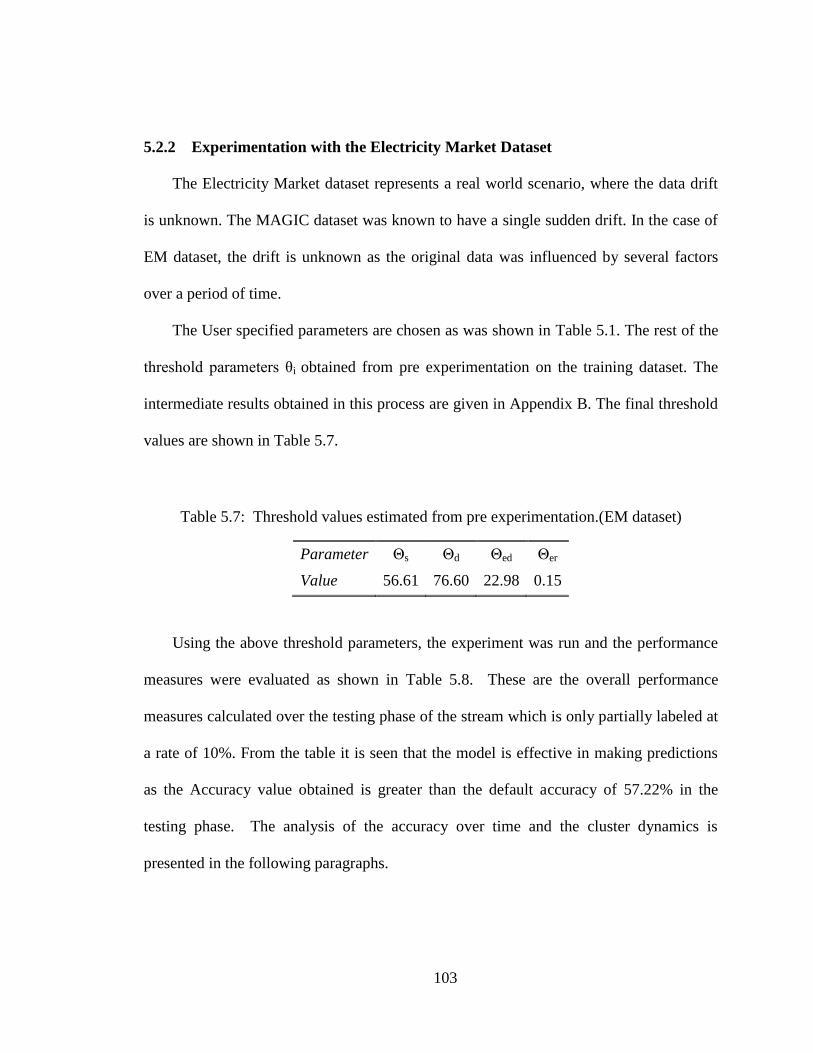
103

5.2.2 Experimentation with the Electricity Market Dataset

The Electricity Market dataset represents a real world scenario, where the data drift

is unknown. The MAGIC dataset was known to have a single sudden drift. In the case of

EM dataset, the drift is unknown as the original data was influenced by several factors

over a period of time.

The User specified parameters are chosen as was shown in Table 5.1. The rest of the

threshold parameters θi obtained from pre experimentation on the training dataset. The

intermediate results obtained in this process are given in Appendix B. The final threshold

values are shown in Table 5.7.

Table 5.7: Threshold values estimated from pre experimentation.(EM dataset)

Parameter Θs Θd Θed Θer

Value 56.61 76.60 22.98 0.15

Using the above threshold parameters, the experiment was run and the performance

measures were evaluated as shown in Table 5.8. These are the overall performance

measures calculated over the testing phase of the stream which is only partially labeled at

a rate of 10%. From the table it is seen that the model is effective in making predictions

as the Accuracy value obtained is greater than the default accuracy of 57.22% in the

testing phase. The analysis of the accuracy over time and the cluster dynamics is

presented in the following paragraphs.

104

Table 5.8: Performance measures on the EM dataset.

Performance Metric Measured Value

Accuracy 73.3969%

Precision 0.814193

Recall 0.744718

Sensitivity 0.814193

Specificity 0.626655

AUC 0.720424

Number of New Models Generated 22

5.2.2.1 Analysis of Performance over Time

In order to understand the progression of the stream and the reaction by the GC3

framework, a time analysis of the stream is performed. This analysis also enables us to

gain insight into the changes in the EM data stream, which is not known prior to the

experimentation. The graph shows the accuracy over time. It also has the list of all

models generated in the course of the stream. Data tips marked on the graph show the

points at which certain models were developed and the corresponding effect on accuracy.

105

Figure 5.3: Accuracy, Recovery Points, list of models generated over time on the EM

dataset.

This plot represents the working of the GC3 framework in a dynamic environment. It

is seen that, whenever there is a considerable dip in the accuracy a new model is

spawned. A few of these Recovery points are labeled in the Figure 5.3. The overall

accuracy stabilizes after a point and this is when the current ensemble is able to monitor

the stream closely and adjust to its changes appropriately.

As seen from the plot, the first model is developed at timestamp 4531, which marks

the beginning of the testing phase and it is the initial_train_timestamp for this

experiment. The remaining models are eventually developed due to a combination of the

cluster dynamics and the drift in the model representation of the cluster ensemble. The

variation in the plot is explained by monitoring the reaction by the GC3 system. The

106

initial variation seen till timestamp 5847 is due to the cluster dynamics, i.e. smaller

clusters combining to form large clusters as the data arrives. The models generated along

with the timestamp at which they are generated are shown in the Figure 5.3. The cluster

dynamics are presented in Figure 5.4, which illustrates the cluster tree’s progression. In

the initial stages, the Cluster 7 and 8 combine to form Cluster 9, which in turn combines

with Cluster 10 to give Cluster 11. Cluster 11 is a stable large cluster which has the bulk

of the models generated in it. 20 models are generated on Cluster 11 over the course of

the stream, with the first model developed at timestamp=5847.

Figure 5.4: Cluster_tree at the end of the EM dataset.

The clusters stabilize soon indicating that there is very less distribution drift in the

system. The 3 models labeled in Figure 5.4 are generated due to the formation of new

107

clusters, with model on cluster 7 being the first model formed at the start of the testing

phase. The remaining 20 models were developed on cluster 11 and are primarily due to

model drift. These models are made necessary by the changes in the data as the stream

progresses. In a real world milieu as represented by the EM dataset, there is usually a

combination of distribution and model drifts, with clusters changing frequently in the

initial stages and model drift being predominant in the later stages of operation.

5.2.2.2 Sensitivity Analysis

In case of the EM dataset, the choice of τ and nb will determine the accuracy and the

number of models produced. A small value of nb will cause more models to be generated

as the model generated will not be adequate to define the new concept. A high value of nb

will cause the drift detection process to be delayed and hence cause a loss in the

accuracy. Tolerance is also closely related to nb, as such it is necessary to evaluate the

sensitivity of the system to these models at the combination of their levels.

Table 5.9: Accuracy Measures at (τ, nb).(EM dataset)

nb\τ 10 15 20

1.5 0.701258 0.699517 0.735391

2 0.717099 0.709889 0.718791

2.5 0.682058 0.717516 0.713077

3 0.698732 0.733969 0.669209

108

Table 5.10: Number of New Models Generated at (τ, nb)(EM dataset).

nb\τ 10 15 20

1.5 53 42 43

2 34 41 32

2.5 42 23 21

3 25 22 23

Table 5.11: Area Under ROC Curve Measures at (τ, nb) (EM dataset).

nb\τ 10 15 20

1.5 0.696349 0.685378 0.72464

2 0.708758 0.702509 0.704773

2.5 0.683328 0.701901 0.703536

3 691053 0.720424 0.646769

From the tables it is observed that the variance in the values is minimal. Also, the

AUC values indicate that the class imbalance does not affect the performance and as such

accuracy is a valid measure for assessing the model. A 95% confidence interval for the

number of models and the accuracy for the EM dataset as evaluated by the GC3

framework is presented in Table 5.12. The Probability plots shown in Figure 5.5 indicate

that the assumption of normality of the data is maintained. The underlying distribution of

both the accuracy and number of models can be approximated to a normal distribution.

Thus, the GC3 model’s performance are not significantly affected by the parameters as

long as they are chosen from the suggested range of 1.5-3 for nb and 10-20% for

tolerance.

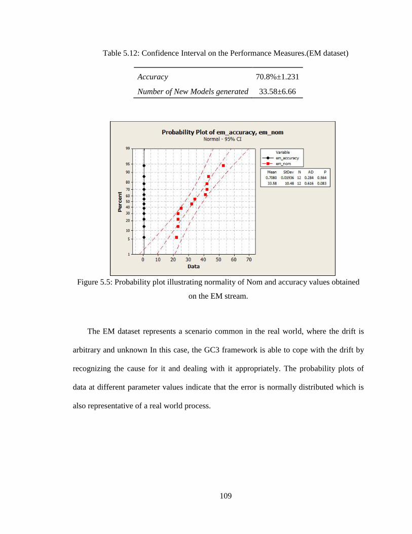
109

Table 5.12: Confidence Interval on the Performance Measures.(EM dataset)

Accuracy 70.8%±1.231

Number of New Models generated 33.58±6.66

Figure 5.5: Probability plot illustrating normality of Nom and accuracy values obtained

on the EM stream.

The EM dataset represents a scenario common in the real world, where the drift is

arbitrary and unknown In this case, the GC3 framework is able to cope with the drift by

recognizing the cause for it and dealing with it appropriately. The probability plots of

data at different parameter values indicate that the error is normally distributed which is

also representative of a real world process.

110

5.3 Comparison of the GC3 Framework with Existing Techniques

In this section the performance of the GC3 Framework is compared with other

existing systems. The first set of comparisons is presented with respect to a traditional

static model with no drift detection capability. The second part presents comparisons

with existing models as described in Chapter 2. The parameter values of Table 5.13 are

chosen for the GC3 framework. These are listed below for the sake of convenience.

Table 5.13: User Specified parameter values for Comparison of GC3 Framework.

Parameter λ Δ τ nb

Value 0.1 5 15 3

5.3.1 Comparison with Traditional Static Models

Here, the performance of the GC3 framework is compared with traditional static

model without drift detection capability. The plot in Figure 5.6 depicts the performance

of the two systems over time for the Magic Dataset. It can be seen that as the time

progresses and drift occurs, the GC3 system adjusts to the change and maintains its

performance with only slight variation. However, since the traditional model has no drift

detection capability, after the occurrence of the drift, the model deteriorates rapidly.

The need for a drift handling system is clearly emphasized by the plot in Figure 5.6.

It shows the performance comparison of the two models on the EM dataset. It is seen that

the traditional model degrades over time, after a time however both models follow similar

trajectories. This is the region where the drift has averaged out the effect and hence

stabilized in accuracy. It is important to observer the initial stage of the graph wherein the

performance of the traditional model decreases. The performance of the GC3 model

111

improves rapidly after it recognizes a drift has occurred and adjusts to it. As such it

maintains a comparatively high accuracy throughout.

Figure 5.6: Comparison of Accuracy over time (MAGIC dataset).

Figure 5.7: Comparison of Accuracy over time (EM dataset).

112

The plots indicate the need for a drift detection capability as the model accuracy will

continue to degrade after the occurrence of a drift. The Table 5.14 summarizes the

performance measures of the two models. The graphs in Figure 5.8 and 5.9 depict the

same.

Table 5.14:Comparison of Performance of Traditional Model and the GC3

Framework(Real World Ddatasets).

Performance

Metric MAGIC Dataset EM Dataset

GC3

Framework

Traditional

Model

GC3

Framework

Traditional

Model

Accuracy 97.1492% 60.9300% 73.3969% 67.9238%

Sensitivity 0.927033 0.000000 0.814193 0.863430

Specificity 1 1.000000 0.626655 0.432846

Precision 0.927033 0.000000 0.814193 0.863430

Recall 1 - 0.744718 0.670672

AUC 0.963517 0.500000 0.720424 0.648138

Nom 3 1 23 1

Figure 5.8:Comparison of performance with Traditional model. (MAGIC dataset).

0.40

0.50

0.60

0.70

0.80

0.90

1.00

Magic Dataset Performance Comparison

GC3 Framework

Traditional Model

113

Figure 5.9: Comparison of performance with Traditional model. (EM dataset).

It can be seen that the GC3 Framework outperforms the traditional model on both the

datasets. This is because both streams have a significant drift and as such the traditional

static model developed on the initial 10% of the stream is soon outdated and causes the

performance to degrade. Although the number of models used by the framework is larger,

it is made necessary by the changes in the stream. These models enable the ensemble to

stay updated and be able to define the current concept in the system.

5.3.2 Comparison with existing ensemble based drift handling systems

In the previous section, a comparison of the GC3 framework with the traditional data

mining technique indicated that there is a need for drift handling systems when dealing

with these real world datasets. In this section, a comparison of the GC3 Framework’s

performance, with that of existing systems designed for handling concept drift, is

0.40

0.45

0.50

0.55

0.60

0.65

0.70

0.75

0.80

0.85

0.90

EM Dataset Comparison

GC3 Framework

Traditional Model

114

presented. The Simple Voting Ensemble (SVE), the Weighted Ensemble [29], and the

Ensemble technique proposed by Woo et al in [34], are used for making the comparison.

These techniques were described in Chapter 2. Both the SVE and WE use consecutive

samples within each chunk to make new classifiers periodically. The SVE uses the

majority voting aggregation technique to arrive at the final prediction, while the WE uses

a weighted majority voting with higher weight given to classifiers which get the highest

accuracy on the most recent chunk. The Woo et al ensemble classifier is based on the

notion of ‘Classification upon Clustering’, with new classifiers formed from dense

regions of samples which do not become a part of any of the existing clusters. The Woo

ensemble classifier does not generate new classifiers within existing clusters. This is one

of its major limitations.

In [34], Woo et al presented the comparison using the SVE and WE technique using

a chunk size of 300. The parameter values for the Woo ensemble were as follows-

training data density for building a classifier θs=300, radius of neighboring area θr=2σ0,

where σ0 is the standard deviation of the initial training data, and λ =0.4 is the labeled

sample rate within the same training data area. It was also suggested to use the Weighted

Sum of F-measures (WSF) as a suitable measure of ensemble accuracy applied for

streaming data in multi classification problem with skewed class distribution. The WSF is

defined as follows:

∑ )

(6.3)

Where, CLASS denotes the set of all the classes, F (ci) is the F- measure of the class

ci. F-measure is the harmonic mean of the Precision and Recall. A value of WSF close to

115

1 is desirable. The weights wi are calculated based on the density of the samples of a

particular class in the dataset as shown in Equation 6.4. Here, ni is the number of sample

of class ci in the testing phase and N is the total size of the testing dataset.

) (6.4)

Apart from the WSF measure described above, the total number of new models

generated (Nom) and the labeling ration (λ) were considered for making a comparison.

The results are derived from [34] and are presented in. Figure 5.10 presents the graphical

representation of the comparison under each metric. For the purpose of comparison the

parameter values as used in Section 5.3.1 are set for the GC3 ensemble. The τ is fixed at

15%, the λ=0.1, Δ=5 and the nb is taken as 3.

Table 5.15: Comparison with Nom, λ and WSF on SVE, WE and Woo ensemble.

Methodology MAGIC Dataset EM Dataset

Nom λ WSF Nom λ WSF

GC3 Framework 2 10% 0.968 22 10% 0.716

Woo et al 6 9% 0.774 6 12% 0.643

SVE 60 99% 0.789 86 99% 0.688

WE 60 99% 0.655 86 99% 0.564

116

Figure 5.10: Comparison of WSF, Nom and λ for GC3 framework, SVE, WE and Woo

ensemble.

0.5

0.6

0.7

0.8

0.9

1

GC3 Woo SVE WE GC3 Woo SVE WE

Magic Dataset EMDatasetWig

hte

d S

um

Of

F m

eas

ure

s(W

SF)

WSF

0.0010.0020.0030.0040.0050.0060.0070.0080.0090.00

100.00

GC3 Woo SVE WE GC3 Woo SVE WE

Magic Dataset EMDataset

Nu

mb

er

of

ne

w m

od

els

ge

ne

rate

d Nom

0.00%

20.00%

40.00%

60.00%

80.00%

100.00%

GC3 Woo SVE WE GC3 Woo SVE WE

Magic Dataset EMDataset

Lab

elin

g R

atio

Labeling Ratio

117

The GC3 Framework gives higher WSF for both the datasets with a comparatively

lower labeling rate. For the MAGIC dataset, the WSF of 0.968 is much higher than its

counterparts with only 2 new models generated. The labeling rate is kept fixed at 10%

and it is much lesser than the SVE and WE which need almost all the data to be labeled.

In case of the EM dataset, a high WSF is produced with only ¼ th

the number of models

used for SVE and WE. However, the number of models used was higher than that used

by Woo et al. This number of models is necessary to generate a high accuracy on the

given data. Using fewer models will cause the EM prediction to be no better than using a

single static classifier as depicted in Figure 5.9. It can be seen here that, GC3 framework

also outperforms the SVE and WE ensemble techniques by a significant margin. When

compared with the Woo model it is seen that, for the same labeling rate, higher prediction

accuracy can be achieved by using the GC3 ensemble.

5.4 Why the GC3 Framework performs better than SVE, WE and Woo

methodology?

The GC3 Framework outperforms the existing ensemble techniques in both the

datasets considered here. As compared to the Woo ensemble methodology, the

framework produced a 25.06% higher WSF value on the MAGIC dataset and 11.35%

higher on the EM dataset, with almost the same labeling ratio (~10%). The reason for this

significant improvement can be attributed to the design of the GC3 framework.

The Woo ensemble makes spherical clusters which, for both datasets, quickly

degrade into one large cluster. Also, it has no model updating capability which leads to a

rapid drop in performance when a drift occurs in an established cluster. Since, the entire

118

data space is formed into one large cluster; a lack of the model updating capability causes

it to be less useful in an environment where the class distribution drift is more prevalent

than data distribution drift. The MAGIC dataset is an example of such type of dataset. As

seen in Figure 5.2, the sample space is represented by one large stable cluster, indicating

little distribution drift. In this case, the Woo ensemble is not able to detect changes in the

class distribution over time. The GC3 framework designed to deal with both the data

distribution drift and the class distribution drift, is able to form multiple models in the

same cluster and make predictions weighted according to the Recentness of the model.

Also, this changeover is swift with only a small loss in accuracy as the new models

developed are once again capable of defining the current state of the cluster. This result in

a 25.06% higher WSF for the GC3 framework as compared to the Woo ensemble.

In case of the EM dataset, after the initial phase of the stream, the traditional model

and the GC3 framework follow similar trajectories indicating that the drift has stabilized.

The major loss in accuracy occurs in the initial phase of the stream if drift is not detected

and handled appropriately. The GC3 framework detects small clusters in this phase as

shown in Figure 5.4, which leads to its rapid rise in accuracy shown in Figure 5.6. The

initial rise in accuracy causes the GC3 Framework to detect and adjust to the change

quickly and as such maintain a better accuracy throughout. The Woo ensemble owing to

its large spherical clusters is not able to capture these distributions that are prevalent in

different regions of the initial stream. Thus, it performs no better than the static model

and consequently does not need additional models in representing the concept. The GC3

framework is able to detect these changes and uses extra models to differentially

represent them to give an 11.35% higher WSF value.

119

The GC3 Framework is a trigger based drift detector which takes action only when

there is need to restore the system’s performance in the wake of a concept drift. As such

it generates models only when needed and generates enough so as to adequately define

the new concept. Thus it produces significantly lesser number of models as compared to

the SVE and WE and shown in Figure 5.10. The GC3 framework produced only 3.3% of

the models generated by SVE and WE on the MAGIC dataset and 25.6% of the models

on the EM dataset, to give a WSF value which is, on average,35.2% higher for the

MAGIC dataset and 15.51% higher on the EM dataset, with only 10% of the data labeled.

This is because the GC3 framework identifies the cause of the drift and takes actions

accordingly so as to produce good results with only the necessary resources, as opposed

to the SVE and WE which generate new models even when the system accuracy is

maintained.

120

CHAPTER 6

CONCLUSION AND FUTURE WORK

In this thesis the problem of Concept Drift in dynamically evolving data streams was

examined. The goal was to create a system which could detect and adjust to changes in

the distribution of stream over time, thereby maintaining its accuracy automatically with

minimum supervision. The methodology proposed by Woo et al in [32] and the Grid

density clustering proposed in [35] were found to be interesting for extension in this

domain. It was believed that the combination of both could result in a robust system

capable of dealing with concept drift.

The proposed GC3 framework was developed to deal with concept drift by

recognizing the cause of drift and responding accordingly. The GC3 framework used the

notion of ‘Classification upon Clustering’ to leverage the power of the grid density based

clustering and that of ensemble classification to build a system capable of detecting

various kinds of drifts in a stream. In order to evaluate the model and to demonstrate its

response to different drifting scenarios, a synthetic data stream called the TJSS stream

was developed. The TJSS stream demonstrated a variety of drift and a time series

analysis of the GC3’s performance confirmed that the framework was able to detect each

of them effectively. The accuracy obtained was 36.55% better than a traditional static

model with no drift detection capability.

121

The GC3 framework outperformed the traditional models in the performance

measures considered in this thesis, thereby emphasizing the need for a drift detection

system for the datasets used. Further, experiments with two real world datasets – the

MAGIC and the EM dataset, were performed and the results were compared with the

existing ensemble methodologies of Woo et al, SVE and WE. The GC3 framework

performed better than all the methodologies for both datasets. The GC3 framework also

outperformed the SVE and the WE approaches producing a WSF of 25.15% with only

14.45% of the models needed, on average. It was shown that GC3 model used

comparatively fewer labeled records when compared with SVE and WE to give a much

better accuracy. When compared with the Woo ensemble, the GC3 framework produced

25.06% higher WSF on the MAGIC dataset, which demonstrated sudden change with

total shift in class prior distributions, and 11.35% higher WSF on the EM dataset, with

unknown drift. Although the number of models generated on the EM dataset was higher

than those produced by Woo et al, it was made necessary to obtain the level of accuracy.

In addition to the better performance of the GC3 framework, it also provided insights

into the dynamics of the stream by analysis of the Cluster_tree data structure. The

Cluster_tree enabled the efficient management of changes to clusters over time and at the

same time provided interpretability for the drift.

The results produced by the GC3 framework are promising to its applicability in a

real world stream classification system. Further applicability to real world streams would

be a topic for future research.

122

Future Work

The evaluation of the GC3 model showed that it was able to effectively tackle two of

the challenges of stream data mining: Robustness and Concept Adaptability. The third

challenge of Scalability is also an important consideration for streaming data. Analysis of

the framework’s scalability is a topic for further work.

The models generated by the cluster ensemble are weighted based on their

Recentness, as such older model are soon outdated and contribute very less to this

aggregation process. These models can be pruned from time to time in order to make

efficient use of the memory. Also, pruning these models will not affect the accuracy

majorly, but would save both time and memory resources. Another improvement to speed

can be provided by replacing the grid_list with a faster access data structure such as a

Hash table or a Red black tree. Since grid_list needs to be scanned on each iteration such

a data organization will greatly speed up the process.

These extensions would enable the GC3 framework to be more efficient and usable

as it is already designed for scalability in large multidimensional input spaces. Use of this

framework for classifying purely categorical variables is also a work for the future.

123

REFERENCES

[1] Tsymbal, Alexey. "The problem of concept drift: definitions and related

work."Computer Science Department, Trinity College Dublin (2004).

[2] Chu, Fang, Yizhou Wang, and Carlo Zaniolo. "An adaptive learning approach for

noisy data streams." Data Mining, 2004. ICDM'04. Fourth IEEE International

Conference on. IEEE, 2004.

[3] Gao, Jing, et al. "A General Framework for Mining Concept-Drifting Data

Streams with Skewed Distributions." SDM. 2007.

[4] Gao, Jing, Wei Fan, and Jiawei Han. "On appropriate assumptions to mine data

streams: Analysis and practice." Data Mining, 2007. ICDM 2007. Seventh IEEE

International Conference on. IEEE, 2007.

[5] Zliobaite, Indre. Learning under concept drift: an overview. Overview”,

Technical report, Vilnius University, 2009 techniques, related areas, applications

Subjects: Artificial Intelligence, 2009.

[6] Hoens, T. Ryan, Robi Polikar, and Nitesh V. Chawla. "Learning from streaming

data with concept drift and imbalance: an overview." Progress in Artificial

Intelligence 1.1 (2012): 89-101.

[7] Quinlan, John Ross. C4. 5: programs for machine learning. Vol. 1. Morgan

kaufmann, 1993.

[8] Domingos, Pedro, and Geoff Hulten. "Mining high-speed data

streams."Proceedings of the sixth ACM SIGKDD international conference on

Knowledge discovery and data mining. ACM, 2000.

[9] Hoeffding, Wassily. "Probability inequalities for sums of bounded random

variables." Journal of the American statistical association 58.301 (1963): 13-30.

[10] Bifet, Albert, and Ricard Gavaldà. "Adaptive learning from evolving data

streams." Advances in Intelligent Data Analysis VIII. Springer Berlin Heidelberg,

2009. 249-260.

124

[11] Hoeglinger, Stefan, and Russel Pears. "Use of hoeffding trees in concept based

data stream mining." Information and Automation for Sustainability, 2007.

ICIAFS 2007. Third International Conference on. IEEE, 2007.

[12] Pfahringer, Bernhard, Geoffrey Holmes, and Richard Kirkby. "New options for

hoeffding trees." AI 2007: Advances in Artificial Intelligence. Springer Berlin

Heidelberg, 2007. 90-99.

[13] Hulten, Geoff, Laurie Spencer, and Pedro Domingos. "Mining time-changing

data streams." Proceedings of the seventh ACM SIGKDD international

conference on Knowledge discovery and data mining. ACM, 2001.

[14] Rai, Piyush, Hal Daumé III, and Suresh Venkatasubramanian. "Streamed

learning: one-pass SVMs." Proceedings of the 21st international jont conference

on Artifical intelligence. Morgan Kaufmann Publishers Inc., 2009.

[15] Alippi, C., and M. Roveri. "Just-in-time adaptive classifiers in non-stationary

conditions." Neural Networks, 2007. IJCNN 2007. International Joint Conference

on. IEEE, 2007.

[16] Widmer, Gerhard, and Miroslav Kubat. "Learning in the presence of concept

drift and hidden contexts." Machine learning 23.1 (1996): 69-101.

[17] Widmer, Gerhard, and Miroslav Kubat. "Effective learning in dynamic

environments by explicit context tracking." Machine Learning: ECML-93.

Springer Berlin Heidelberg, 1993.

[18] Lazarescu, Mihai M., Svetha Venkatesh, and Hung H. Bui. "Using multiple

windows to track concept drift." Intelligent Data Analysis 8.1 (2004): 29-59.

[19] Klinkenberg, Ralf. "Learning drifting concepts: Example selection vs. example

weighting." Intelligent Data Analysis 8.3 (2004): 281-300.

[20] Breiman, Leo. "Bagging predictors." Machine learning 24.2 (1996): 123-140.

[21] Breiman, Leo. "Random forests." Machine learning 45.1 (2001): 5-32.

[22] Freund, Yoav, and Robert E. Schapire. "Experiments with a new boosting

algorithm." ICML. Vol. 96. 1996.

[23] Kuncheva, Ludmila I. "Classifier ensembles for changing environments."

Multiple classifier systems. Springer Berlin Heidelberg, 2004. 1-15.

[24] Littlestone, Nick, and Manfred K. Warmuth. "The weighted majority

algorithm." Foundations of Computer Science, 1989., 30th Annual Symposium

on. IEEE, 1989.

125

[25] Street, W. Nick, and YongSeog Kim. "A streaming ensemble algorithm (SEA)

for large-scale classification." Proceedings of the seventh ACM SIGKDD

international conference on Knowledge discovery and data mining. ACM, 2001.

[26] Oza, Nikunj C. "Online bagging and boosting." Systems, man and cybernetics,

2005 IEEE international conference on. Vol. 3. IEEE, 2005.

[27] Kolter, Jeremy Z., and Marcus A. Maloof. "Dynamic weighted majority: A new

ensemble method for tracking concept drift." Data Mining, 2003. ICDM 2003.

Third IEEE International Conference on. IEEE, 2003.

[28] Kolter, J. Zico, and Marcus A. Maloof. "Dynamic weighted majority: An

ensemble method for drifting concepts." The Journal of Machine Learning

Research 8 (2007): 2755-2790.

[29] Wang, Haixun, et al. "Mining concept-drifting data streams using ensemble

classifiers." Proceedings of the ninth ACM SIGKDD international conference on

Knowledge discovery and data mining. ACM, 2003.

[30] Nishida, Kyosuke, Koichiro Yamauchi, and Takashi Omori. "ACE: Adaptive

classifiers-ensemble system for concept-drifting environments." Multiple

Classifier Systems. Springer Berlin Heidelberg, 2005. 176-185.

[31] Katakis, Ioannis, Grigorios Tsoumakas, and Ioannis Vlahavas. "Incremental

Clustering for the Classification of Concept-Drifting Data Streams."

[32] Ryu, Joung Woo, Mehmed Kantardzic, and Chamila Walgampaya. "Ensemble

Classifier Based on Misclassified Streaming Data." Proc. of the 10th IASTED Int.

Conf. on Artificial Intelligence and Applications, Austria. 2010.

[33] Kantardzic, Mehmed, Joung Woo Ryu, and Chamila Walgampaya. "Building a

new classifier in an ensemble using streaming unlabeled data." Trends in Applied

Intelligent Systems. Springer Berlin Heidelberg, 2010. 77-86.

[34] Ryu, Joung Woo, Mehmed M. Kantardzic, and Myung-Won Kim."Efficiently

Maintaining the Performance of an Ensemble Classifier in Streaming Data."

Convergence and Hybrid Information Technology. Springer Berlin Heidelberg,

2012. 533-540.

[35] Chen, Yixin, and Li Tu. "Density-based clustering for real-time stream data."

Proceedings of the 13th ACM SIGKDD international conference on Knowledge

discovery and data mining. ACM, 2007.

126

[36] Tu, Li, and Yixin Chen. "Stream data clustering based on grid density and

attraction." ACM Transactions on Knowledge Discovery from Data (TKDD) 3.3

(2009): 12.

[37] Sun, Xin, and Yu Cathy Jiao. "pGrid: Parallel Grid-Based Data Stream

Clustering with MapReduce.".

[38] Aggarwal, Charu C., et al. "A framework for clustering evolving data

streams."Proceedings of the 29th international conference on Very large data

bases-Volume 29. VLDB Endowment, 2003.

[39] Guha, Sudipto, et al. "Clustering data streams." Foundations of computer

science, 2000. proceedings. 41st annual symposium on. IEEE, 2000.

[40] O'callaghan, Liadan, et al. "Streaming-data algorithms for high-quality

clustering." Data Engineering, 2002. Proceedings. 18th International Conference

on. IEEE, 2002.

[41] Nasraoui, Olfa, Carlos Rojas, and Cesar Cardona. "A framework for mining

evolving trends in web data streams using dynamic learning and retrospective

validation." Computer Networks 50.10 (2006): 1488-1512.

[42] Beringer, Jürgen, and Eyke Hüllermeier. "Online clustering of parallel data

streams." Data & Knowledge Engineering 58.2 (2006): 180-204.

[43] Dean, Jeffrey, and Sanjay Ghemawat. "MapReduce: a flexible data processing

tool." Communications of the ACM 53.1 (2010): 72-77.

[44] Harries, Michael, and New South Wales. "Splice-2 comparative evaluation:

Electricity pricing." (1999).

[45] Gama, Joao, et al. "Learning with drift detection." Advances in Artificial

Intelligence–SBIA 2004. Springer Berlin Heidelberg, 2004. 286-295.

[46] Bache, K., and M. Lichman. "UCI machine learning repository." School of

Information and Computer Science, University of California, Irvine, CA.

http://archive. ics. uci. edu/ml. Last accessed on May 30 (2013): 2013.

[47] Masud, Mohammad M., et al. "A practical approach to classify evolving data

streams: Training with limited amount of labeled data." Data Mining, 2008.

ICDM'08. Eighth IEEE International Conference on. IEEE, 2008.

[48] Kuncheva, Ludmila I., Christopher J. Whitaker, and A. Narasimhamurthy. "A

case-study on naïve labelling for the nearest mean and the linear discriminant

classifiers." Pattern Recognition 41.10 (2008): 3010-3020.

127

[49] “Electricity Market Dataset” available from,

http://moa.cms.waikato.ac.nz/datasets/ .

[50] Wikipedia contributors. "Manhattan distance." Wikipedia, The Free

Encyclopedia. Wikipedia, The Free Encyclopedia, 19 Dec. 2003. Web. 7 Jul.

2013.

[51] Wikipedia contributors. "C4.5 algorithm." Wikipedia, The Free Encyclopedia.

Wikipedia, The Free Encyclopedia, 4 Mar. 2013. Web. 7 Jul. 2013.

[52] Wikipedia contributors. "Binary classification." Wikipedia, The Free

Encyclopedia. Wikipedia, The Free Encyclopedia, 18 Mar. 2013. Web. 7 Jul.

2013.

[53] Kantardzic, Mehmed. Data mining: concepts, models, methods, and algorithms.

John Wiley & Sons, 2011.

[54] Surowiecki, James. The wisdom of crowds. Random House Digital, Inc., 2005.

[55] Ahmadi, Zahra, and Hamid Beigy. "Semi-supervised ensemble learning of data

streams in the presence of concept drift." Hybrid Artificial Intelligent Systems.

Springer Berlin Heidelberg, 2012. 526-537.

128

APPENDIX A

COMPONENTS OF THE TJSS STREAM

The TJSS stream was introduced in Chapter 4. The details of each of the clusters and

their evolving characteristics are described in this section. The figure below is the same

as Figure 4.2, and is presented here for the sake of convenience.

Figure A.1: Components of the TJSS stream

There are 5 distinct clusters in the Figure A.1. A description of each of the cluster A-

E is presented below.

129

Cluster A: The Cluster A is as shown in the Figure A.2. The cluster appears from

the start of the stream and has a stable model defined. As time progresses, the

cluster extends downwards from both its sides while maintain the same model

throughout. This is depicted in the figures below:

a) b)

Figure A.2: Evolution of Cluster A(TJSS Stream).

This cluster embodies a distribution drift, in which the model is constant however the

probability P(x) as described in Section 2.1.1, changes as the time proceeds. Thus an

established cluster might encompass more area as the time progresses with the same

concept.

Cluster B: The Cluster B is a simple rectangle with a stable model and

distribution. However, as the time progresses and concept drift occur, there is a

total reversal of the class distribution in its region. As described in Section 2.1 this

type of drift is known as a virtual drift, wherein the distribution of point’s changes

but the model boundary is intact.

130

a) b)

Figure A.3: Evolution of Cluster B(TJSS Stream).

This cluster would enable to demonstrate the ability of the methodology in predicting

the class labels of a region which has changed over time. It is necessary to have a

forgetting factor incorporated to make such a kind of differentiation.

Cluster C: Cluster C is split into C1 and C2. The cluster C1 is initially present in

the stream and as time progresses as the Cluster C1 appears. It is initially a

disjoint cluster but with the passage of time it combines to form one whole cluster

C.

a) b) c)

Figure A.4: Evolution of Cluster C (TJSS Stream).

131

As seen from the Figure A.4, the Cluster C1 initially is a well-defined concept and it

has an arch shape. The grid based clustering algorithm should be able to capture this

shape of the cluster. As time progresses the cluster C2 appears. At time stamp 16840 the

second plot is observed. This cluster has all samples of only one class and it is regarded

as an individual cluster. At time 17640, the next snapshot is taken and it is seen that the

Cluster C1 and C2 get combined to form one large cluster. At this point both the models

of the existing cluster are maintained and at the same time there is a need for an overall

model as the global model for this cluster is a bit more complex than the individual

cluster models and needs to be updated based on this new data. The proposed grid based

clustering methodology needs to account for dynamic combinations of clusters each with

their own established prediction models.

Cluster D: This cluster is also present from the start of the stream. As the concept

drift occurs in the stream, the cluster starts to extend in both directions opposite to

each other. Also, these extensions depict a concept opposite to the prevailing

concept in the cluster. This cluster depicts an important aspect of drift. It

demonstrates a type of drift which has both a model drift P(y|x) and a distribution

drift P(x) as described in Equation 2.1. Also, the change in shape of the cluster is

evident in this cluster. The snapshot of Cluster D as taken at timestamps: 13200,

20040 is shown in Figure A.5.

132

a) b)

Figure A.5: Evolution of Cluster D(TJSS Stream).

Cluster E: This cluster is absent from the stream in the beginning. Samples start

appearing in this region starting at timestamp 20040. It evolves as shown in the

Figure A.6.

a) b) c)

Figure A.6: Evolution of Cluster E(TJSS Stream).

This cluster enables us to judge the performance of the model in case of new unseen

clusters with an unknown model in the stream. It depicts primarily a general form of a

drift where there is a distribution drift and a model drift and the extent of drift maybe

unknown.

Random Patches R1,2,3: Apart from the above mentioned clusters, there are three

patches of randomly occurring data points into grids, which are not dense enough

to become clusters, however these still need to be clustered based on the existing

models. These patches appear as shown in Figure A.1.

133

APPENDIX B

PARAMETER ESTIMATION USING PRE EXPERIMENTATION

The methodology to estimate parameter values using pre experimentation was

described in Section 3.6. The intermediate results used in evaluating the final threshold

values for the experiments in Sections 4.2 and 5.2 are presented below.

Experiment on the Synthetic Dataset: The TJSS stream

Table B.1: User Specified Parameter Values (TJSS Stream)

Parameter λ Δ τ nb

Value 0.1 20 0.25 1.25

Table B.2: Intermediate Results from pre experiment.

Parameter Evaluation Value

Initial Subset Size (Ntr) Training ratio*Dataset Size(N) 2566

Number of Active grids(na) Size(grid_list) 33

Average active density(ρavg) ρavg =Ntr/na 77.75

Size of Dense Data (Ndt) ∑ )

1775

Number of dense active grids (nda) ∑

22

Average density of active grid ρden_avg ρden_avg=Ndt/nda 80.68

134

Table B.3: Final Threshold values (TJSS Stream)

Parameter Θs Θd Θed Θer

Value 60.5 100.85 15.1 0.25

Experiments with real world datasets

Experiments on the Magic Dataset

Table B.4: User Specified Parameter Values(MAGIC Dataset)

Parameter λ Δ τ nb

Value 0.1 5 15 3

Table B.5: Intermediate Results from pre experiment(MAGIC Dataset)

Parameter Evaluation Value

Initial Subset Size (Ntr) Training ratio*Dataset Size(N) 1902

Number of Active grids(na) Size(grid_list) 411

Average active density(ρavg) ρavg =Ntr/na 4.63

Size of Dense Data (Ndt) ∑ )

1422

Number of dense active grids (nda) ∑

49

Average density of active grid ρden_avg ρden_avg=Ndt/nda 29.02

Table B. 6: Final Threshold values (MAGIC Dataset)

Parameter Θs Θd Θed Θer

Value 24.67 33.37 10.01 0.15

135

Experiments on the EM Dataset

Table B.7: User specified parameter values (EM dataset).

Parameter λ Δ τ nb

Value 0.1 5 15 3

Table B. 8: Intermediate Results from pre experiment (EM dataset).

Parameter Evaluation Value

Initial Subset Size (Ntr) Training ratio*Dataset Size(N) 4531

Number of Active grids(na) Size(grid_list) 122

Average active density(ρavg) ρavg =Ntr/na 37.14

Size of Dense Data (Ndt) ∑ )

3930

Number of dense active grids (nda) ∑

59

Average density of active grid ρden_avg ρden_avg=Ndt/nda 66.61

Table B.9: Final Threshold values (EM dataset).

Parameter Θs Θd Θed Θer

Value 56.61 76.60 22.98 0.15

136

CURRICULUM VITAE

NAME: Tegjyot Singh Sethi

ADDRESS: Department of Computer Engineering and Computer Science

University of Louisville

Louisville, KY 40292

EDUCATION:

M.S., Computer Science

University of Louisville

est. 2013

B.Tech., Computer Science and Engineering

GITAM University, Visakhapatnam, India

2012

PROFESSIONAL EXPERIENCE:

2012-2013 Graduate Teaching Assistant, University of Louisville

2011 Software Engineer Intern at Visakhapatnam Steel Plant, India.

PUBLICATIONS:

1. Hari, Ch VMK, Tegjyot Singh Sethi, et al. "SEEPC: A Toolbox for

Software Effort Estimation using Soft Computing

Techniques." International Journal of Computer Applications 31.4

(2011): 12-19.

2. Hari, C. V. M. K., Tegjyot Singh Sethi, et al. “CPN-a hybrid model for

software cost estimation.” Recent Advances in Intelligent Computational

Systems (RAICS), 2011 IEEE. IEEE, 2011.

3. Sethi, Tegjyot Singh, et al. "Cluster Analysis & Pso for Software Cost

Estimation." Information Technology and Mobile Communication.

Springer Berlin Heidelberg, 2011. 281-286.

137

Undergraduate Research:

Sethi, Tegjyot Singh. “SIPPSS- Swarm Intelligence based Prediction of

Protein Secondary Structure”, GITAM University, Visakhapatnam, India

(2012).

AWARDS:

2013 CECS Master of Science Award, University of Louisville

2012 Winner of STPI-IMU Young Talent Search In Computer Programming

In Maritime Domain, India

2011 Second Place in 7th

National IT Aptitude Test, India.