The Second-Order Bias and Mean Squared Error ofEstimators in Time Series Models∗

Yong Bao†

Department of EconomicsUniversity of California, Riverside

Aman Ullah‡

Department of EconomicsUniversity of California, Riverside

August 14, 2003

Abstract

We develop the analytical results on the second-order bias and mean squared error (MSE)of estimators in time series. These results provide a unified approach to developing theproperties of a large class of estimators in the linear and nonlinear time series models andthey are valid for both the normal and non-normal sample of observations, and where theregressors are stochastic. The estimators included are the generalized method of moments,maximum likelihood, least squares, and other extremum estimators. Our general results areapplied to a wide variety of econometric models. Numerical results for some of these modelsare presented.

Keywords: Higher-order moments; Stochastic expansion; Time series; Quadratic form

JEL Classification: C10, C22, C32

∗We would like to thank Gloria Gonzalez-Rivera, Emma Iglesias and Victoria Zinde-Walsh for helpfulcomments. Bao thanks the UCR Chancellor Fellowship and Ullah thanks the UCR Academic Senate forresearch support. All remaining errors are our own.

†Department of Economics, University of California, Riverside, CA, 92521, (909) 788-7998, e-mail: yong-bao@mail.ucr.edu.

‡Corresponding Author: Department of Economics, University of California, Riverside, CA, 92521, (909)827-1591, Fax: (909) 787-5685, e-mail: aman.ullah@ucr.edu.

1 Introduction

There is an extensive literature on the analytical finite sample properties of econometric

estimators and test statistics in linear models, see Nagar (1959), Anderson and Sawa (1973,

1979), Basmann (1974), Sargan (1974, 1976), Phillips (1977), Rothenberg (1984), Ullah and

Srivastava (1994), and Ullah (2002), among others. In contrast, not much work has been

done on the finite sample properties of the nonlinear statistics, although see Roberston and

Fryer (1970), Amemiya (1980), Chesher and Spady (1989), Cordeiro and McCullagh (1991),

Koenker et al. (1992), and Newy and Smith (2001). However, most of these works are for

some specific estimators and there is little with the dependent observations for nonlinear

cases, although see Cordeiro and Klein (1994) and Linton (1997). Recently, Rilstone et al.

(1996) developed the large-n second-order bias and mean squared error (MSE) of a class of

nonlinear estimators. Nevertheless, their results are for the i.i.d. sample so they are not

applicable to the models with dependent observations, for example, the time series models.

In this paper, we extend the second-order bias and MSE results of Rilstone et al. (1996)

for the time series dependent observations. These results provide a unified way of developing

the properties of a given class of estimators in the linear and nonlinear time series models.

The estimators included are the generalized method of moments (GMM), maximum likeli-

hood (ML), least squares (LS) and other extremum estimators, and the two step estimators

which involve a nuisance parameter. Our results are also valid for both the normal and non-

normal sample of observations, and where the regressors are stochastic. Next, in a special

case of the ML estimators (MLE) we also show that our bias result reduces to that of the

bias of MLE in Cox and Snell (1968) for the i.i.d. case and its extension in Cordeiro and

Klein (1994) for the dependent observations. However, we note that our bias result is for

a general class of estimators including the ML as a special case and that Cox and Snell’s

(1968) approach does not provide the MSE of estimators. Furthermore, as an application of

our general results, we develop the second-order bias and MSE for some time series models.

These include the AR(1) model, structural model with AR(1) errors, VAR model, MA(1)

1

model, partial adjustment model, and absolute regression model.

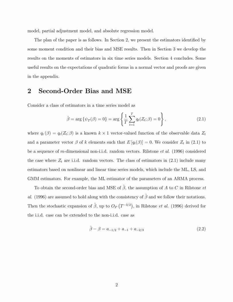
The plan of the paper is as follows. In Section 2, we present the estimators identified by

some moment condition and their bias and MSE results. Then in Section 3 we develop the

results on the moments of estimators in six time series models. Section 4 concludes. Some

useful results on the expectations of quadratic forms in a normal vector and proofs are given

in the appendix.

2 Second-Order Bias and MSE

Consider a class of estimators in a time series model as

β = arg ψT (β) = 0 = arg(1

T

TXt=1

qt(Zt; β) = 0

), (2.1)

where qt (β) = qt(Zt;β) is a known k × 1 vector-valued function of the observable data Ztand a parameter vector β of k elements such that E [qt(β)] = 0. We consider Zt in (2.1) to

be a sequence of m-dimensional non-i.i.d. random vectors. Rilstone et al. (1996) considered

the case where Zt are i.i.d. random vectors. The class of estimators in (2.1) include many

estimators based on nonlinear and linear time series models, which include the ML, LS, and

GMM estimators. For example, the ML estimator of the parameters of an ARMA process.

To obtain the second-order bias and MSE of β, the assumption of A to C in Rilstone et

al. (1996) are assumed to hold along with the consistency of β and we follow their notations.

Then the stochastic expansion of β, up to OP¡T−3/2

¢, in Rilstone et al. (1996) derived for

the i.i.d. case can be extended to the non-i.i.d. case as

β − β = a−1/2 + a−1 + a−2/3 (2.2)

2

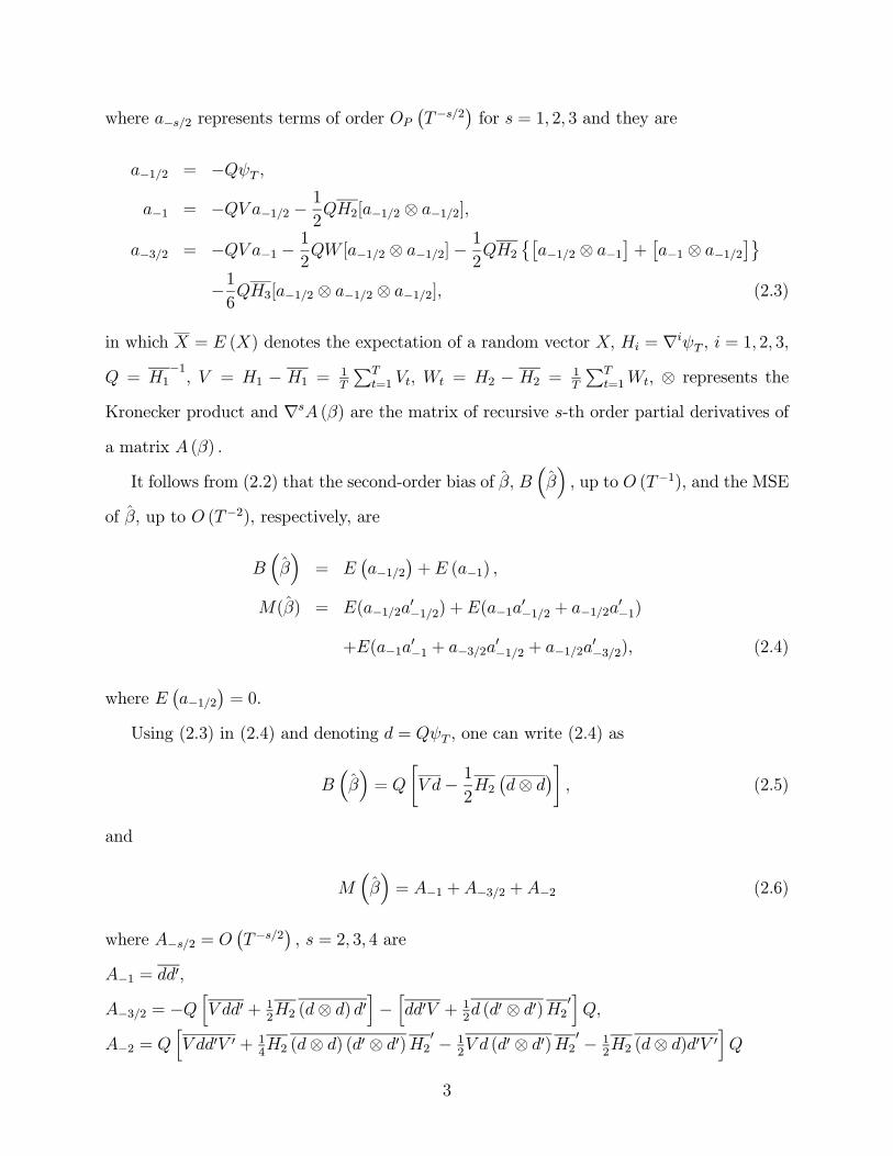
where a−s/2 represents terms of order OP¡T−s/2

¢for s = 1, 2, 3 and they are

a−1/2 = −QψT ,

a−1 = −QV a−1/2 − 12QH2[a−1/2 ⊗ a−1/2],

a−3/2 = −QV a−1 − 12QW [a−1/2 ⊗ a−1/2]− 1

2QH2

©£a−1/2 ⊗ a−1

¤+£a−1 ⊗ a−1/2

¤ª−16QH3[a−1/2 ⊗ a−1/2 ⊗ a−1/2], (2.3)

in which X = E (X) denotes the expectation of a random vector X, Hi = ∇iψT , i = 1, 2, 3,Q = H1

−1, V = H1 − H1 = 1

T

PTt=1 Vt, Wt = H2 − H2 = 1

T

PTt=1Wt, ⊗ represents the

Kronecker product and ∇sA (β) are the matrix of recursive s-th order partial derivatives ofa matrix A (β) .

It follows from (2.2) that the second-order bias of β, B³β´, up to O (T−1), and the MSE

of β, up to O (T−2), respectively, are

B³β´= E

¡a−1/2

¢+E (a−1) ,

M(β) = E(a−1/2a0−1/2) +E(a−1a0−1/2 + a−1/2a

0−1)

+E(a−1a0−1 + a−3/2a0−1/2 + a−1/2a

0−3/2), (2.4)

where E¡a−1/2

¢= 0.

Using (2.3) in (2.4) and denoting d = QψT , one can write (2.4) as

B³β´= Q

·V d− 1

2H2¡d⊗ d¢¸ , (2.5)

and

M³β´= A−1 +A−3/2 +A−2 (2.6)

where A−s/2 = O¡T−s/2

¢, s = 2, 3, 4 are

A−1 = dd0,

A−3/2 = −QhV dd0 + 1

2H2 (d⊗ d) d0

i−hdd0V + 1

2d (d0 ⊗ d0)H20

iQ,

A−2 = QhV dd0V 0 + 1

4H2 (d⊗ d) (d0 ⊗ d0)H20 − 1

2V d (d0 ⊗ d0)H20 − 1

2H2 (d⊗ d)d0V 0

iQ

3

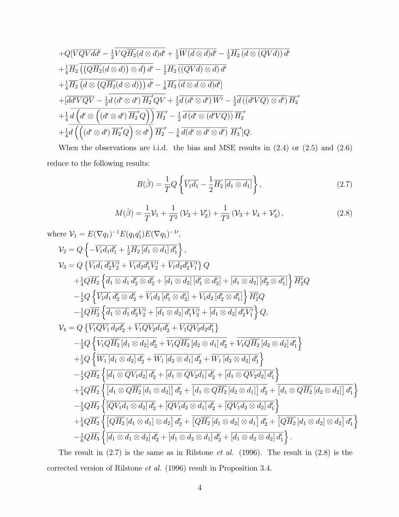
+Q[V QV dd0 − 12V QH2(d⊗ d)d0 + 1

2W (d⊗ d)d0 − 1

2H2 (d⊗ (QV d)) d0

+14H2¡¡QH2(d⊗ d)

¢⊗ d¢ d0 − 12H2 ((QV d)⊗ d) d0

+14H2¡d⊗ ¡QH2(d⊗ d)¢¢ d0 − 1

6H3 (d⊗ d⊗ d)d0]

+[dd0V QV − 12d (d0 ⊗ d0)H20QV + 1

2d (d0 ⊗ d0)W 0 − 1

2d ((d0V Q)⊗ d0)H20

+14d³d0 ⊗

³(d0 ⊗ d0)H20Q

´´H2

0 − 12d (d0 ⊗ (d0V Q))H20

+14d³³(d0 ⊗ d0)H20Q

´⊗ d0

´H2

0 − 16d(d0 ⊗ d0 ⊗ d0) H30]Q.

When the observations are i.i.d. the bias and MSE results in (2.4) or (2.5) and (2.6)

reduce to the following results:

B(β) =1

TQ

½V1d1 − 1

2H2 [d1 ⊗ d1]

¾, (2.7)

M(β) =1

TV1 + 1

T 2(V2 + V 02) +

1

T 2(V3 + V4 + V 04) , (2.8)

where V1 = E(∇q1)−1E(q1q01)E(∇q1)−10,V2 = Q

n−V1d1d01 + 1

2H2 [d1 ⊗ d1] d01

o,

V3 = Q©V1d1 d02V

02 + V1d2d

01V

02 + V1d2d

02V

01

ªQ

+14QH2

nd1 ⊗ d1 d02 ⊗ d02 + [d1 ⊗ d2] [d01 ⊗ d02] + [d1 ⊗ d2] [d02 ⊗ d01]

oH 02Q

−12QnV1d1 d02 ⊗ d02 + V1d2 [d01 ⊗ d02] + V1d2 [d02 ⊗ d01]

oH 02Q

−12QH 0

2

nd1 ⊗ d1 d02V 02 + [d1 ⊗ d2] d01V 02 + [d1 ⊗ d2] d02V 01

oQ,

V4 = Q©V1QV1 d2d02 + V1QV2d1d

02 + V1QV2d2d

01

ª−12QnV1QH2 [d1 ⊗ d2] d02 + V1QH2 [d2 ⊗ d1] d02 + V1QH2 [d2 ⊗ d2] d01

o+12QnW1 [d1 ⊗ d2] d02 +W1 [d2 ⊗ d1] d02 +W1 [d2 ⊗ d2] d01

o−12QH2

n[d1 ⊗QV1d2] d02 + [d1 ⊗QV2d1] d02 + [d1 ⊗QV2d2] d01

o+14QH2

n£d1 ⊗QH2 [d1 ⊗ d2]

¤d02 +

£d1 ⊗QH2 [d2 ⊗ d1]

¤d02 +

£d1 ⊗QH2 [d2 ⊗ d2]

¤d01o

−12QH2

n[QV1d1 ⊗ d2] d02 + [QV1d2 ⊗ d1] d02 + [QV1d2 ⊗ d2] d01

o+14QH2

n£QH2 [d1 ⊗ d1]⊗ d2

¤d02 +

£QH2 [d1 ⊗ d2]⊗ d1

¤d02 +

£QH2 [d1 ⊗ d2]⊗ d2

¤d01o

−16QH3

n[d1 ⊗ d1 ⊗ d2] d02 + [d1 ⊗ d2 ⊗ d1] d02 + [d1 ⊗ d2 ⊗ d2] d01

o.

The result in (2.7) is the same as in Rilstone et al. (1996). The result in (2.8) is the

corrected version of Rilstone et al. (1996) result in Proposition 3.4.

4

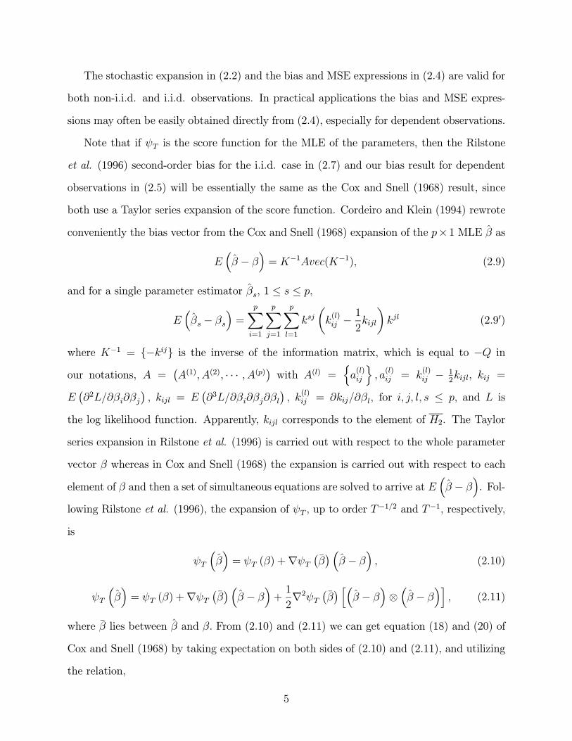
The stochastic expansion in (2.2) and the bias and MSE expressions in (2.4) are valid for

both non-i.i.d. and i.i.d. observations. In practical applications the bias and MSE expres-

sions may often be easily obtained directly from (2.4), especially for dependent observations.

Note that if ψT is the score function for the MLE of the parameters, then the Rilstone

et al. (1996) second-order bias for the i.i.d. case in (2.7) and our bias result for dependent

observations in (2.5) will be essentially the same as the Cox and Snell (1968) result, since

both use a Taylor series expansion of the score function. Cordeiro and Klein (1994) rewrote

conveniently the bias vector from the Cox and Snell (1968) expansion of the p×1 MLE β as

E³β − β

´= K−1Avec(K−1), (2.9)

and for a single parameter estimator βs, 1 ≤ s ≤ p,

E³βs − βs

´=

pXi=1

pXj=1

pXl=1

ksjµk(l)ij −

1

2kijl

¶kjl (2.90)

where K−1 = −kij is the inverse of the information matrix, which is equal to −Q in

our notations, A =¡A(1), A(2), · · · , A(p)¢ with A(l) = n

a(l)ij

o, a(l)ij = k

(l)ij − 1

2kijl, kij =

E¡∂2L/∂βi∂βj

¢, kijl = E

¡∂3L/∂βi∂βj∂βl

¢, k

(l)ij = ∂kij/∂βl, for i, j, l, s ≤ p, and L is

the log likelihood function. Apparently, kijl corresponds to the element of H2. The Taylor

series expansion in Rilstone et al. (1996) is carried out with respect to the whole parameter

vector β whereas in Cox and Snell (1968) the expansion is carried out with respect to each

element of β and then a set of simultaneous equations are solved to arrive at E³β − β

´. Fol-

lowing Rilstone et al. (1996), the expansion of ψT , up to order T−1/2 and T−1, respectively,

is

ψT

³β´= ψT (β) +∇ψT

¡β¢ ³

β − β´, (2.10)

ψT

³β´= ψT (β) +∇ψT

¡β¢ ³

β − β´+1

2∇2ψT

¡β¢ h³

β − β´⊗³β − β

´i, (2.11)

where β lies between β and β. From (2.10) and (2.11) we can get equation (18) and (20) of

Cox and Snell (1968) by taking expectation on both sides of (2.10) and (2.11), and utilizing

the relation,

5

E³∇ψT

¡β¢ ³

β − β´´= E

¡∇ψT ¡β¢¢E ³β − β´+ Cov

³∇ψT

¡β¢, β − β

´= E

¡∇ψT ¡β¢¢E ³β − β´+¡−∇ψ−1T ¢Cov ¡ψT ,∇ψT ¡β¢¢+ o (T−1)

= E (∇ψT )E³β − β

´+¡−∇ψ−1T ¢Cov (ψT ,∇ψT ) + o (T−1) , and

E³∇2ψT

¡β¢ h³

β − β´⊗³β − β

´i´= E

¡∇2ψT ¡β¢¢E ³h³β − β´⊗³β − β

´i´+ o (T−1)

= E¡∇2ψT ¢E ³h³β − β

´⊗³β − β

´i´+ o (T−1) ,

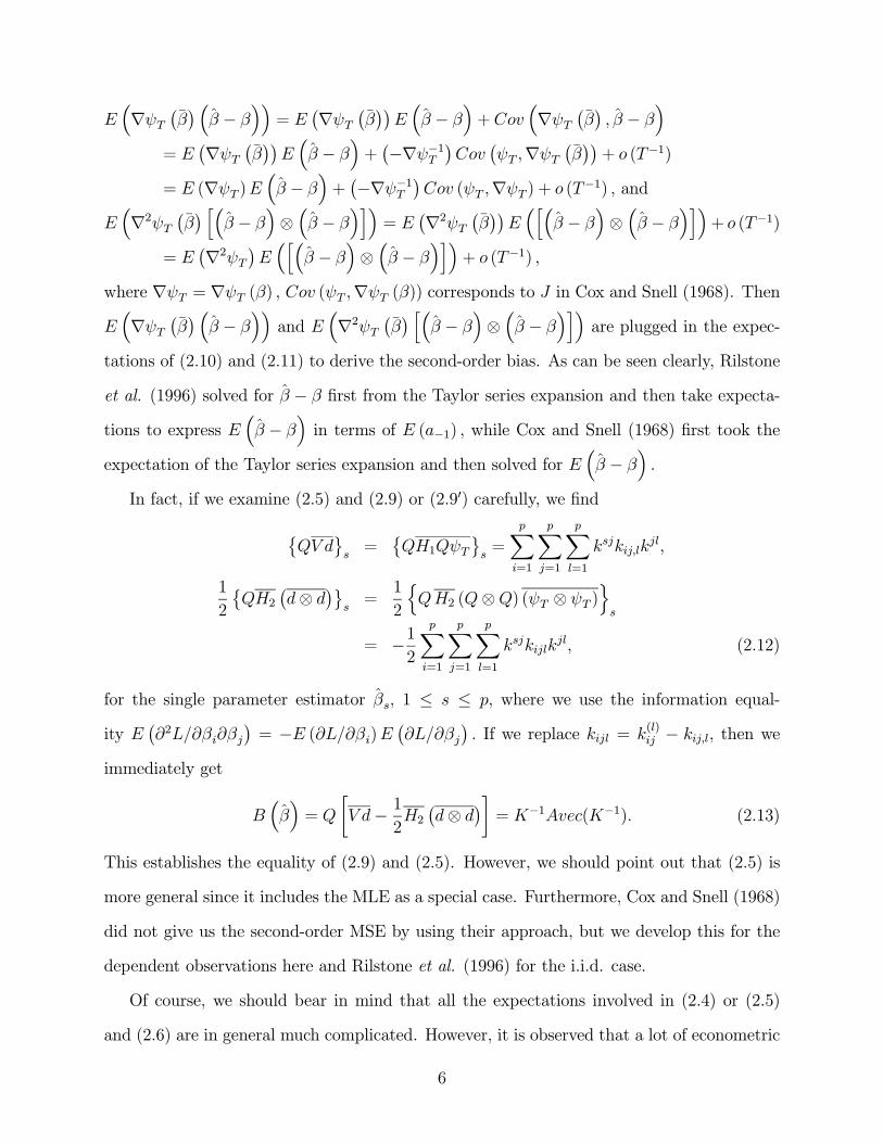
where ∇ψT = ∇ψT (β) , Cov (ψT ,∇ψT (β)) corresponds to J in Cox and Snell (1968). ThenE³∇ψT

¡β¢ ³

β − β´´

and E³∇2ψT

¡β¢ h³

β − β´⊗³β − β

´i´are plugged in the expec-

tations of (2.10) and (2.11) to derive the second-order bias. As can be seen clearly, Rilstone

et al. (1996) solved for β − β first from the Taylor series expansion and then take expecta-

tions to express E³β − β

´in terms of E (a−1) , while Cox and Snell (1968) first took the

expectation of the Taylor series expansion and then solved for E³β − β

´.

In fact, if we examine (2.5) and (2.9) or (2.90) carefully, we find

©QV d

ªs=

©QH1QψT

ªs=

pXi=1

pXj=1

pXl=1

ksjkij,lkjl,

1

2

©QH2

¡d⊗ d¢ª

s=

1

2

nQH2 (Q⊗Q) (ψT ⊗ ψT )

os

= −12

pXi=1

pXj=1

pXl=1

ksjkijlkjl, (2.12)

for the single parameter estimator βs, 1 ≤ s ≤ p, where we use the information equal-

ity E¡∂2L/∂βi∂βj

¢= −E (∂L/∂βi)E

¡∂L/∂βj

¢. If we replace kijl = k

(l)ij − kij,l, then we

immediately get

B³β´= Q

·V d− 1

2H2¡d⊗ d¢¸ = K−1Avec(K−1). (2.13)

This establishes the equality of (2.9) and (2.5). However, we should point out that (2.5) is

more general since it includes the MLE as a special case. Furthermore, Cox and Snell (1968)

did not give us the second-order MSE by using their approach, but we develop this for the

dependent observations here and Rilstone et al. (1996) for the i.i.d. case.

Of course, we should bear in mind that all the expectations involved in (2.4) or (2.5)

and (2.6) are in general much complicated. However, it is observed that a lot of econometric

6

estimators are derived from some quadratic moment conditions. Then some well known

results on the expectations of quadratic forms in a normal or nonnormal vector can be used

for our purpose. In the following section, we use these results extensively for most of the

examples.

3 Illustrations

In this section, we give the application of our second-order bias and MSE results to some time

series models. These include the AR(1) model, structural model with AR(1) errors, VAR

model, MA(1) model, partial adjustment model, and absolute regression model. Here we do

not attempt to give an exhaustive list of all interesting econometric models, for example,

the ARCH model of Engle (1982).1 The approach, however, is unified, and is practically

applicable as long as we can take expectations on the derivatives (up to third order) of the

moment function used for estimation. We note that some results (e.g., AR(1)) are readily

available through other methods in the literature and are consistent with our results or

degenerate as our special cases, but most results are new through our method and are easy

to implement numerically.

3.1 AR Model

Consider an AR(1) model

yt = βyt−1 + εt, (3.1)

where |β| < 1, εt is i.i.d. N(0,σ2ε) and t = 1, 2, ..., T. Denote y = (y1, y2, · · · , yT )0 , then

y ∼ N (0,Σ) , where Σ = σtt0 is a T × T matrix with σtt0 = σ2εβ|t−t0|/

¡1− β2

¢for t,

t0 = 1, 2, ..., T.

1We find that the second-order bias for ML estimator in ARCH(1) model isQnV1d1 − 1

2H2 [d1 ⊗ d1]o/T−

Q³P

i>j Vidj

´/T, which is of course equivalent to the result using (2.9). Iglesias and Phillips (2001, 2002)

derived the result using (2.9) directly. We got the same result in an early version of this paper. To savespace, we do not repeat the result in this paper. The MSE result is more involved and is in our futureresearch agenda.

7

It is well known that the OLS estimator of β is equivalent to the (conditional) ML

estimator. That is, to estimate, we use the following moment condition

ψT =1

T − 1TXt=2

yt−1εt =1

T − 1y0Cy = 0, (3.2)

where C = ctt0 is a T × T matrix with ctt0 = −β for t = t0 = 1, 2, · · · , T − 1, ctt0 = 1/2 ift = t0 + 1 or t = t0 − 1 and it is 0 otherwise. Therefore, we have

H1 = ∇ψT =y0C1yT − 1 , H2 = H3 = 0,

Q = H1−1=

µtrC1Σ

T − 1¶−1

, V = H1 −H1, W = 0, (3.3)

where C1 = ∇C = ∇ctt0 with ∇ctt0 = −1 for t = t0 = 1, 2, · · · , T − 1 and otherwiseit is 0. Using (3.3) in (2.4) or (2.5) and (2.6) and noting that tr (CΣ) = 0 we obtain the

second-order bias of β, up to O (T−1) , and MSE, up to O (T−2) , as

B³β´=

1

(T − 1)2Q2λ11,

M³β´=

6Q2

(T − 1)2λ20 +2Q3

(T − 1)3¡1 + 3Q2

¢λ21 +

3Q4

(T − 1)4λ22, (3.4)

where λrs = E [(y0Cy)r · (y0C1y)s] for r, s = 0, 1, 2 are given in Appendix A.2. Note that in

Appendix A.2 we further simplify, up to o (T−1) ,

B³β´=−2β(T − 1) , (3.5)

which is consistent with Phillips (1977), for instance.

Remark 1: If we include some nonstochastic exogenous regressors, for example, X, in the

AR(1) model, then the extension is straightforward. Also, we can generalize the case to an

AR(p) model with some exogenous regressors, as long as we can rewrite

1

T − jTX

t=j+1

ytyt−j = y0Njy, j = 0, 1, · · · , p. (3.6)

See, for example, Kiviet and Phillips (1993).

8

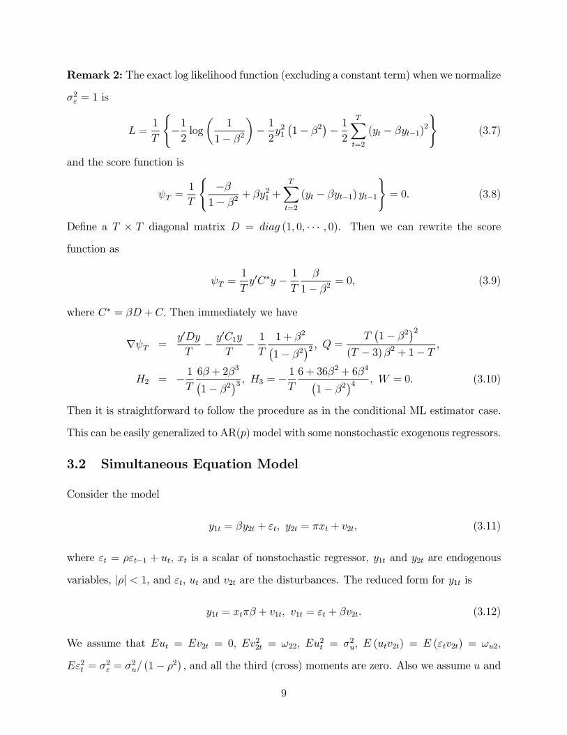
Remark 2: The exact log likelihood function (excluding a constant term) when we normalize

σ2ε = 1 is

L =1

T

(−12log

µ1

1− β2

¶− 12y21¡1− β2

¢− 12

TXt=2

(yt − βyt−1)2

)(3.7)

and the score function is

ψT =1

T

(−β1− β2

+ βy21 +TXt=2

(yt − βyt−1) yt−1

)= 0. (3.8)

Define a T × T diagonal matrix D = diag (1, 0, · · · , 0). Then we can rewrite the scorefunction as

ψT =1

Ty0C∗y − 1

T

β

1− β2= 0, (3.9)

where C∗ = βD + C. Then immediately we have

∇ψT =y0DyT− y

0C1yT− 1

T

1 + β2¡1− β2

¢2 , Q = T¡1− β2

¢2(T − 3)β2 + 1− T ,

H2 = − 1T

6β + 2β3¡1− β2

¢3 , H3 = − 1T 6 + 36β2 + 6β4¡1− β2

¢4 , W = 0. (3.10)

Then it is straightforward to follow the procedure as in the conditional ML estimator case.

This can be easily generalized to AR(p) model with some nonstochastic exogenous regressors.

3.2 Simultaneous Equation Model

Consider the model

y1t = βy2t + εt, y2t = πxt + v2t, (3.11)

where εt = ρεt−1 + ut, xt is a scalar of nonstochastic regressor, y1t and y2t are endogenous

variables, |ρ| < 1, and εt, ut and v2t are the disturbances. The reduced form for y1t is

y1t = xtπβ + v1t, v1t = εt + βv2t. (3.12)

We assume that Eut = Ev2t = 0, Ev22t = ω22, Eu2t = σ2u, E (utv2t) = E (εtv2t) = ωu2,

Eε2t = σ2ε = σ2u/ (1− ρ2) , and all the third (cross) moments are zero. Also we assume u and

9

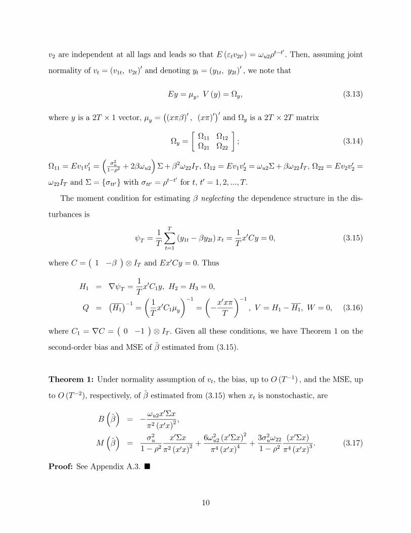
v2 are independent at all lags and leads so that E (εtv2t0) = ωu2ρt−t0 . Then, assuming joint

normality of vt = (v1t, v2t)0 and denoting yt = (y1t, y2t)

0 , we note that

Ey = µy, V (y) = Ωy, (3.13)

where y is a 2T × 1 vector, µy =¡(xπβ)0 , (xπ)0

¢0and Ωy is a 2T × 2T matrix

Ωy =

·Ω11 Ω12Ω21 Ω22

¸; (3.14)

Ω11 = Ev1v01 =

³σ2u1−ρ2 + 2βωu2

´Σ+ β2ω22IT , Ω12 = Ev1v

02 = ωu2Σ+ βω22IT , Ω22 = Ev2v

02 =

ω22IT and Σ = σtt0 with σtt0 = ρt−t0for t, t0 = 1, 2, ..., T.

The moment condition for estimating β neglecting the dependence structure in the dis-

turbances is

ψT =1

T

TXt=1

(y1t − βy2t)xt =1

Tx0Cy = 0, (3.15)

where C =¡1 −β ¢⊗ IT and Ex0Cy = 0. Thus

H1 = ∇ψT =1

Tx0C1y, H2 = H3 = 0,

Q =¡H1¢−1

=

µ1

Tx0C1µy

¶−1=

µ−x

0xπT

¶−1, V = H1 −H1, W = 0, (3.16)

where C1 = ∇C =¡0 −1 ¢ ⊗ IT . Given all these conditions, we have Theorem 1 on the

second-order bias and MSE of β estimated from (3.15).

Theorem 1: Under normality assumption of vt, the bias, up to O (T−1) , and the MSE, up

to O (T−2), respectively, of β estimated from (3.15) when xt is nonstochastic, are

B³β´= −ωu2x

0Σx

π2 (x0x)2,

M³β´=

σ2u1− ρ2

x0Σx

π2 (x0x)2+6ω2u2 (x

0Σx)2

π4 (x0x)4+3σ2uω221− ρ2

(x0Σx)

π4 (x0x)3. (3.17)

Proof: See Appendix A.3. ¥

10

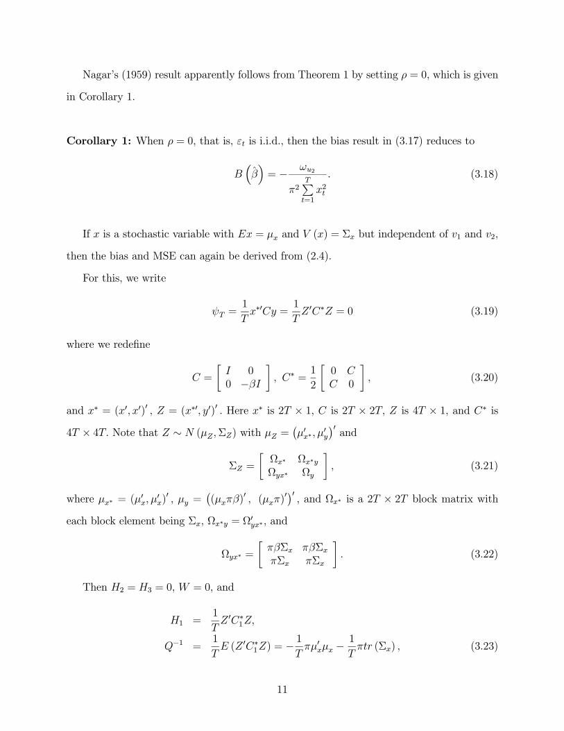
Nagar’s (1959) result apparently follows from Theorem 1 by setting ρ = 0, which is given

in Corollary 1.

Corollary 1: When ρ = 0, that is, εt is i.i.d., then the bias result in (3.17) reduces to

B³β´= − ωu2

π2TPt=1

x2t

. (3.18)

If x is a stochastic variable with Ex = µx and V (x) = Σx but independent of v1 and v2,

then the bias and MSE can again be derived from (2.4).

For this, we write

ψT =1

Tx∗0Cy =

1

TZ 0C∗Z = 0 (3.19)

where we redefine

C =

·I 00 −βI

¸, C∗ =

1

2

·0 CC 0

¸, (3.20)

and x∗ = (x0, x0)0 , Z = (x∗0, y0)0 . Here x∗ is 2T × 1, C is 2T × 2T, Z is 4T × 1, and C∗ is4T × 4T. Note that Z ∼ N (µZ ,ΣZ) with µZ =

¡µ0x∗, µ

0y

¢0and

ΣZ =

·Ωx∗ Ωx∗yΩyx∗ Ωy

¸, (3.21)

where µx∗ = (µ0x, µ

0x)0 , µy =

¡(µxπβ)

0 , (µxπ)0¢0 , and Ωx∗ is a 2T × 2T block matrix with

each block element being Σx, Ωx∗y = Ω0yx∗, and

Ωyx∗ =

·πβΣx πβΣxπΣx πΣx

¸. (3.22)

Then H2 = H3 = 0, W = 0, and

H1 =1

TZ 0C∗1Z,

Q−1 =1

TE (Z 0C∗1Z) = −

1

Tπµ0xµx −

1

Tπtr (Σx) , (3.23)

11

where C∗1 is C∗ with C replaced by

C1 =

·0 00 −IT

¸. (3.24)

Note that both C∗ and C∗1 are symmetric.

Theorem 2: Under normality assumption of vt, the bias, up to O (T−1) , and the MSE, up

to O (T−2), respectively, of β estimated from (3.15) when xt is stochastic, are

B³β´=

(−ωu2tr (ΣΣx)− ωu2µ0xΣµx)

π2 [µ0xµx + tr (Σx)]2 ,

M³β´= 3

Q4

T 4λ11 − 2Q

2

T 2λ10, (3.25)

where λij = Eh(Z 0C∗Z)2i (Z 0C∗1Z)

2jifor i, j = 0, 1.

Proof: See Appendix A.3. ¥

Note that (3.17) is just a special case of (3.25). Corollary 2 and 3 given below give the

second-order bias results for some specific cases of xt.

Corollary 2: If xt follows an AR(1) process as xt = ρxxt−1+ηt, |ρx| < 1, ηt ∼ i.i.d.¡0, σ2η

¢,

σ2x = σ2η/ (1− ρ2x) , then the bias result in (3.25) reduces to

B³β´=

−ωu2

Tσ2x + TPt=1

TPt0=1

t6=t0(ρρxσ

2x)t−t0

π2 (Tσ2x)

2 . (3.26)

Corollary 3: If xt or εt is i.i.d. with mean zero, then the bias result in (3.26) reduces to

B³β´= − ωu2

Tπ2Ex21. (3.27)

12

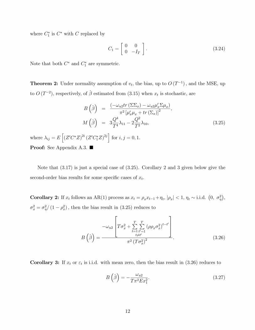
Note that (3.27) encompasses the result in Rilstone et al. (1996) in that even though εt

is an AR(1) process the bias result in Rilstone et al. (1996) will hold as long as xt is i.i.d.

with mean zero.

3.3 VAR Model

Consider the following VAR(1) model½y1t = β11y1,t−1 + β12y2,t−1 + ε1ty2t = β21y1,t−1 + β22y2,t−1 + ε2t

,

µε1tε2t

¶∼ N (0,Ω) , (3.28)

where Ω = ωij, i, j = 1, 2.Define yt = (y1t, y2t)

0 , B =¡(β11, β12)

0 , (β21,β22)0¢0 , εt = (ε1t, ε2t)

0 , then we can com-

pactly write

yt = Byt−1 + εt. (3.29)

We assume that the process is covariance stationary, that is, for all λ satisfying |I2λ−B| = 0,|λ| < 1. For nonstationary VAR models, see Phillips (1987). In particular, this implies

that |β11| < 1, |β22| < 1, |β12β21| < 1. Denote Γ0 = E (yty0t) , Γj = E

¡yty

0t−j¢, Γ−j =

E (yt−jy0t) = Γ0j. Let vec (A) be a column vector of all the columns of A stacked from the

first one to the last one. We know that vec (Γ0) = (I4 −B ⊗B)−1 vec (Ω) and Γj = BjΓ0.

Therefore, yt ∼ N¡0, vec−1

£(I4 −B ⊗B)−1 vec (Ω)

¤¢. If we stack all observations as y =

(y01, y02, · · · , y0T )0 , then we have y ∼ N (0,Σ), where Σ is the 2T×2T variance-variance matrix

with the tt0th element being Bt−t0Γ0 if t ≥ t0 and Bt0−tΓ00 if t < t0 for t, t0 = 1, 2, ..., T.

It is well known that the maximum likelihood estimators of each single equation is the

same as the OLS estimators. As in Section 3.1, if we properly define Cij, i, j = 1, 2, then

we have the following moment condition for β ≡ vec (B)

ψT =1

T − 1TXt=2

qt =1

T − 1TXt=2

vec [(yt −Byt−1) y0t] =1

T − 1

y0C11yy0C21yy0C12yy0C22y

= 0, (3.30)

13

where

C11 =

µ02(T−1)×2 AA02×2 02×2(T−1)

¶− β11

µAA 02(T−1)×202×2(T−1) 02×2

¶− β12

µBB 02(T−1)×202×2(T−1) 02×2

¶,

C21 =

µ02(T−1)×2 BB02×2 02×2(T−1)

¶− β21

µAA 02(T−1)×202×2(T−1) 02×2

¶− β22

µBB 02(T−1)×202×2(T−1) 02×2

¶,

C12 =

µ02(T−1)×2 CC02×2 02×2(T−1)

¶− β11

µCC 02(T−1)×202×2(T−1) 02×2

¶− β12

µDD 02(T−1)×202×2(T−1) 02×2

¶,

C22 =

µ02(T−1)×2 DD02×2 02×2(T−1)

¶− β21

µCC 02(T−1)×202×2(T−1) 02×2

¶− β22

µDD 02(T−1)×202×2(T−1) 02×2

¶,

where the 2 (T − 1) × 2 (T − 1) matrices AA, BB, CC, and DD are block diagonal with

the block element aa =¡(1, 0)0 , (0, 0)0

¢0, bb =

¡(0, 1)0 , (0, 0)0

¢0, cc =

¡(0, 0)0 , (1, 0)0

¢0, and

dd =¡(0, 0) , (0, 1)0

¢0, respectively.

Define C11 = C(1)11 − β11C

(2)11 − β12C

(3)11 , where C

(l)11 , l = 1, 2, 3, represents the lth matrix

part in the definition of C11 in (3.30). Similar definitions are used for C21, C12, and C22.

Note that y0C(3)11 y = y0C(2)12 y, y

0C(3)21 y = y0C(2)22 y.

Immediately we have

∇ψT = H1 = − 1

T − 1

y0C(2)11 y 0 y0C(3)11 y 0

0 y0C(2)21 y 0 y0C(3)21 yy0C(2)12 y 0 y0C(3)12 y 0

0 y0C(2)22 y 0 y0C(3)22 y

,H2 = H3 =W = 0. (3.31)

The results on quadratic forms in Appendix A.1 then can be used here to evaluate the

second-order bias and MSE of β. Denote E³y0C(l)ij y

´= tr

h³C(l)ij + C

(l)0ij

´Σ/2

i= λ

(l)ij ,

E³y0Cijy · y0C(l)mny

´= 2tr

h¡Cij + C

0ij

¢Σ³C(l)mn + C

(l)0mn

´Σ/4

i+ tr

£¡Cij + C

0ij

¢Σ/2

¤×trh³C(l)mn + C

(l)0mn

´Σ/2

i= µ

(l)ijmn for i, j,m, n = 1, 2 and λ

(3)i1 λ

(2)i2 − λ

(2)i1 λ

(3)i2 = φi for i = 1, 2,

then it is easy to verify the bias result as given in Theorem 3.

Theorem 3: The bias , up to O (T−1), of β estimated from (3.30) in VAR(1) model (3.28)

is

B³βi1

´=

ξiφ2i, B

³βi2

´=

ηiφ2i, i = 1, 2, (3.32)

14

where

ξi =³µ(3)i2i2 − µ(3)i2i1

´λ(2)i1 λ

(3)i1 +

³µ(2)i2i1 − µ(3)i1i2

´λ(3)i1 λ

(2)i2 + µ

(2)i1i2λ

(3)i2 λ

(3)i1 + µ

(3)i1i1λ

(2)i2 λ

(3)i2

−µ(2)i1i1³λ(3)i2

´2− µ(2)i2i2

³λ(3)i1

´2,

ηi =³µ(3)i1i2 − µ(3)i2i1

´λ(2)i1 λ

(2)i2 +

³µ(2)i2i2 − µ(2)i1i2

´λ(2)i1 λ

(3)i1 + µ

(2)i1i1λ

(2)i2 λ

(3)i2 + µ

(2)i2i1λ

(3)i1 λ

(2)i2

−µ(3)i1i1³λ(2)i2

´2− µ(3)i2i2

³λ(2)i1

´2.

Proof: Substitute (3.30) and (3.31) into (2.5) and use the results on quadratic forms in

Appendix A.1. ¥

Here we do not give explicitly expressions for the second-order MSE. However, it is

straightforward to write a computer program to do the evaluation numerically.

Table 1 gives some numerical results for different sample sizes whenB =¡(0.8, 0.3)0 , (0.2, 0.5)0

¢0and

¡(0.1, 0.4)0 , (0.4, 0.3)0

¢0, where eigenvalues refer to those of the parameter matrix B

and we normalize Ω =¡(1, ρ)0 , (ρ, 1)0

¢0.We tried many other different B’s, whose results are

available upon request. Three outstanding points worthy of mentioning are that i) increase

of sample size will significantly reduce the second-order bias and MSE; ii) the higher ρ, the

larger the second-order MSE, which implies that even though the OLS estimators are con-

sistent, the correlation between disturbance terms across equations will cause imprecision

of the OLS estimators; iii) the difference between the second-order and first-order results

is not insignificant for small samples we have considered, and it seems that the first-order

variance, which is equal to the first-order MSE, usually underestimates the second-order

variance,

µM³β´−B

³β´2¶

, as well as the seond-order MSE. Of course, the first-order

variance can be calculated from Ω ⊗ Γ0 (see Hamilton, 1994, p. 299), which is equal to

A−1 is our expression. Since we normalize Ω =¡(1, ρ)0 , (ρ, 1)0

¢0, the first-order variance is

the same for the parameter estimators in the same row of the variance matrix of vec³B´.

Also, we should emphasize that our results are only approximations. For high |ρ| around0.9, we do encounter some second-order MSE with negative values (represented by “/” in

Table 1) or very large unrealistic values around two hundred in small samples, which though

15

is consistent with the fact that our results are asymptotic second-order results.

Remark 3: We can easily generalize to VAR(p) model of n variables, as long as we can

write

TXk=l+1

yi,kyj,k−l = y0Nijky, i, j ≤ n, l ≤ p. (3.33)

3.4 MA Model

Consider the simplest case

yt = εt − βεt−1, |β| < 1, (3.34)

where we normalize εt ∼ i.i.d. N (0, 1) . Define y = (y1, · · · , yt, yt+1, · · · , yT )0 . FollowingHamilton (1994), we have the averaged sample (conditional) log likelihood function, exclud-

ing a constant term, L = − 1T

PTt=1

ε2t2, where εt = yt + βyt−1 + · · ·+ βt−1y1 =

Pt−1i=0 aiyt−i ≡

y0At with ai = βi and

At = At (β) =

at−1, · · · , a1, a0, 0, · · · , 0| z T−t zeros

0

(3.35)

Then we have

∂εt∂θ

= y0Bt,∂2εt

∂θ2= y0Ct,

∂3εt

∂θ3= y0Ut,

∂4εt

∂θ4= y0Vt, (3.36)

where

Bt =∂At∂β, Ct =

∂2At

∂β2, Ut =

∂3At

∂β3, Vt =

∂4At

∂β4, (3.37)

and

qt = −µ∂εt∂β

¶εt = −y0BtA0ty,

∇qt = −µ∂2εt

∂β2

¶εt −

µ∂εt∂β

¶2= −y0CtA0ty − y0BtB0ty,

∇2qt = −µ∂3εt

∂β3

¶εt − 3

µ∂2εt

∂β2

¶µ∂εt∂β

¶= −y0UtA0ty − 3y0CtB0ty,

∇3qt = −µ∂4εt

∂β4

¶εt − 4

µ∂3εt

∂β3

¶µ∂εt∂β

¶− 3

µ∂2εt

∂β2

¶2= −y0VtA0ty − 4y0UtB0ty − 3y0CtC 0ty. (3.38)

16

In matrix notation, we have

ψT =1

Ty0Ny, Hi =

1

Ty0Niy, i = 1, 2, 3, (3.39)

where N = −A0B, N1 = −A0C − B0B, N2 = −A0U − 3B0C, N3 = −A0V − 4B0U − 3C 0C,A = (A1, A2, · · · , AT ) and similarly for B, C, U, V. Note that y is normally distributed withmean 0 and variance-covariance matrix Σ such that it has tt0th element 1 + β2 when t = t0,

−β when |t− t0| = 1, and 0 elsewhere, for t, t0 = 1, 2, · · · , T. With these notations, we usethe results on quadratic forms in Appendix A.1 to derive the second-order bias and MSE of

β. However, we should bear in mind that if we write εt = y0At in stead of εt =

P∞i=0 aiyt−i,

then it is not necessary that E¡a−1/2

¢= 0 in (2.4), but plima−1/2 = 0. The asymptotic

expansion in Rilstone et al. (1996) is nevertheless valid as long as we have√T -consistency

of the estimator β, together with their assumptions A to C.2 Therefore, instead of (2.5), we

use the bias expression in (2.4) directly with E¡a−1/2

¢ 6= 0. The MSE expression given by(2.6), on the other hand, is still valid here. Theorem 4 gives a closed-form formula for the

bias based on the above observation.

Theorem 4: The bias, up to O (T−1), of the conditional ML estimator β for model (3.34)

is

B³β´=

tr (N∗Σ) · tr (N∗1Σ) + 2tr (N

∗ΣN∗1Σ)

[tr (N∗1Σ)]

2 − 2tr (N∗Σ)

tr (N∗1Σ)

−tr (N∗2Σ) ·

£(trN∗Σ)2 + 2tr

¡(N∗Σ)2

¢¤2 [tr (N∗

1Σ)]3 , (3.40)

where N∗i =

Ni+N 0i

2, i = 0, 1, 2, N0 = N, N

∗0 = N

∗.

Proof: Substitute (3.39) into (2.4) and use the results on quadratic forms in Appendix A.1.

¥

2We can of course generalize for any g√T -consistent estimator, g > 0. But (2.3), (2.5) and (2.6) then have

to be modified accordingly.

17

As for M³β´, we do not report the explicit result here. But it is very easy to write a

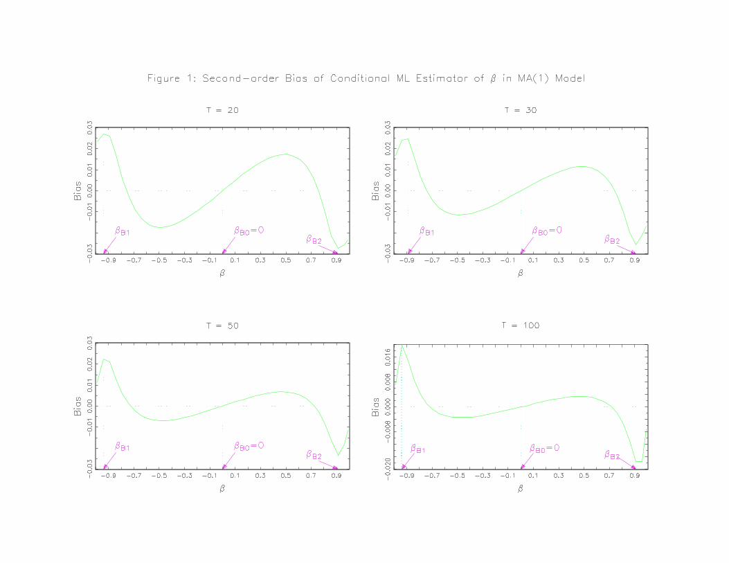
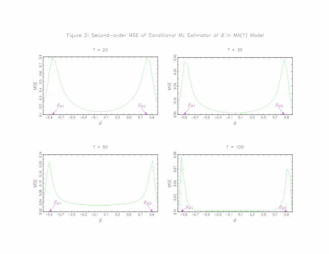
computer program to evaluate it. Figure 1 plots B³β´and Figure 2 plots M

³β´against β

for given sample size T.We see clearly the following patterns for B³β´andM

³β´: i) B

³β´

and M³β´reduces significantly as sample size increases and β is almost unbiased even for

a sample size as small as 20; ii) the second-order bias behaves sinusoidally for β between

(βB1,βB2) and the magnitude of it is approximately symmetric around the point βB0 = 0,

at which the second-order bias is zero; iii)the absolute bias reaches two peaks at βB1 for

β < 0 and at βB2 for β > 0; iv) the second-order MSE is approximately symmetric around

the point where β = 0; v) starting from the origin, the second-order MSE monotonically

increases as the magnitude of β increases until it reaches two peaks at βM1 for β < 0 and

βM2 for β > 0, and then decreases. The exact values of βB1, βB2, βM1, and βM2 can read

from Figure 1 and Figure 2.

Of course, we should point out that as |β| approaches one, the initial values of y for theconditional ML estimator are not negligible in small samples and hence we may cast some

doubt on the second-order results built upon the conditional ML condition when |β| is closeto one.

Remark 4: In principle, this can be generalized to an MA(q) model. Instead of using

quadratic forms in y, we use the normal vector ε directly. For simplicity, consider, for

example, an MA(2) model, yt = εt+θ1εt−1+θ2εt−2. Again, we have the log likelihood function

L = −PTt=1 ε

2t/2T, with εt = yt−θ1εt−1−θ2εt−2. Here we set initial values ε0 = ε−1 = 0. Note

that qt is 2×1,∇qt is 2×2,∇2qt is 2×4, and∇3qt is 2×8.All the expectations of cross productswill boil down to the form of cross products of E (∂4ε/∂θi∂θj∂θk∂θl) , 1 ≤ i, j, k, l ≤ 2, orof lower order. For example, consider E

¡∂4ε/∂θ41

¢. From εt = yt − θ1εt−1 − θ2εt−2 we have

∂εt/∂θ1 = −εt−1−θ1∂εt−1/∂θ1−θ2∂εt−2/∂θ1. Rewrite it as εt−1 = −∂εt/∂θ1−θ1∂εt−1/∂θ1−θ2∂εt−2/∂θ1. Therefore, we have ε = A1∂ε/∂θ1, where A1 is T ×T such that its tt0th elementis equal to −θ1 if t = t0, −1 if t0 = t + 1, −θ2 if t = t0 + 1, and 0 elsewhere, for t,

t0 = 1, 2, · · · , T . Then ∂ε/∂θ1 = A−11 ε = C1ε for C1 = A−11 . Invertibility will guarantee

18

that A1 is nonsingular. Next, from εt−1 = −∂εt/∂θ1 − θ1∂εt−1/∂θ1 − θ2∂εt−2/∂θ1 we have

∂εt−1/∂θ1 = −∂2εt/∂θ21−∂εt−1/∂θ1−θ1∂2εt−1/∂θ21−θ2∂2εt−2/∂θ21. Rewrite it as ∂εt−1/∂θ1 =−12

¡∂2εt/∂θ

21 + θ1∂

2εt−1/∂θ21 + θ2∂2εt−2/∂θ21

¢. Then we can find some matrix C2 such that

∂2ε/∂θ21 = C2∂ε/∂θ1 = C2C1ε. Carrying on this step we can get ∂3ε/∂θ31 = C3∂

2ε/∂θ21 =

C3C2C1ε, and ∂4ε/∂θ41 = C4∂3ε/∂θ31 = C4C3C2C1ε. Therefore, all the expectations of cross

products of E (∂4ε/∂θi∂θj∂θk∂θl) will essentially take some quadratic form in the normal

vector ε. As a result, the standard procedure in Section 3.1 is applicable here.

Remark 5: We can easily extend to the case of an MA(q) with mean µy = x0tβ. If we

combine with Section 3.1, we can generally evaluate a general ARMA process with mean

µy = x0tβ. In essence, we can express the relevant expectations of quadratic forms in the

normal vector (y0, ε0)0 .

Remark 6: We restrict |β| < 1 because our exercise is for the conditional ML estimator. Itwould be more interesting to extend the exercise to unconditional ML estimator, regardless

of whether β is associated with an invertible representation or not. The difficulty of this

exercise is that there is no appropriate way to handle the expectations of the score function

and its derivatives up to third order. We defer this to our future research.

3.5 Partial Adjustment Model

Let y∗t = xtβ + εt be the desired level of some economic variable. The partial adjustment

model describes an adjustment equation yt − yt−1 = (1− γ) (y∗t − yt−1). See Brown (1952)and Lovell (1961) for consumption model of habit persistence. The econometric regression

equation is obtained by substituting the first equation into the adjustment equation and

solving for yt

yt = γyt−1 + (1− γ)βxt + εt = γyt−1 + δxt + εt, (3.41)

where δ = β (1− γ) . For simplicity we assume xt to be an i.i.d. normal scalar and εt ∼N (0,σ2ε). Suppose E (xt) = µx, V (xt) = σ2x, and x is uncorrelated with ε. Note that

even though γ and δ can be estimated consistently and efficiently by OLS as this model is

19

intrinsically linear, the inference about β = δ/ (1− γ) is not so straightforward. Here we try

to derive B³β´and M

³β´.

The OLS estimator needs the following moment condition

ψT =1

T − 1µ PT

t=2 εtyt−1PTt=2 εtxt

¶=

1

T − 1µy0Cy − (1− γ)βx0Ayx0Dy − (1− γ)βx0Bx

¶= 0, (3.42)

where A is T × T with tt0th element equal to 1 if t − t0 = 1 and 0 elsewhere, B is T × Twith tt0th element equal to 1 if t = t0 ≥ 2 and 0 elsewhere, C is T × T with tt0th elementequal to −γ if t = t0 ≤ T − 1, 1/2 if |t− t0| = 1, and 0 elsewhere, for t, t0 = 1, 2, · · · , T, andD = B − γA.

Then we have

∇ψT = H1 =1

T − 1µ − (1− γ)x0Ay −y0C1y + βx0Ay− (1− γ)x0Bx −x0Ay + βx0Bx

¶,

∇2ψT = H2 =1

T − 1µ0 x0Ay x0Ay 00 x0Bx x0Bx 0

¶,

∇3ψT = H3 = 0. (3.43)

where C1 is T × T with tt0th element equal to 1 if t = t0 = 1, 2, · · · , T − 1, and 0 elsewhereTherefore, we can follow the same procedure as in Section 3.1. The only difference is

that we will encounter some bilinear forms like x0Ay. For this we can define y∗ = (x0, y0)0,

then (3.42) and (3.43) can be rewritten as

ψT =1

T − 1µy∗0C∗y∗ − (1− γ)βy∗0A∗y∗

y∗0D∗y∗ − (1− γ)βy∗0B∗y∗

¶= 0, (3.420)

and

∇ψT = H1 =1

T − 1µ − (1− γ) y∗0A∗y∗ −y∗0C∗1y∗ + βy∗0A∗y∗

− (1− γ) y∗0B∗y∗ −y∗0A∗y∗ + βy∗0B∗y∗

¶,

∇2ψT = H2 =1

T − 1µ0 y∗0A∗y∗ y∗0A∗y∗ 00 y∗0B∗y∗ y∗0B∗y∗ 0

¶, (3.430)

where

A∗ =1

2

µ0 AA 0

¶, B∗ =

µB 00 0

¶, C∗ =

µ0 00 C

¶,

C∗1 =

µ0 00 C1

¶, D∗ =

1

2

µ0 DD 0

¶, (3.44)

20

and y∗ ∼ N (µ,Σ) , where

µ =

µµxτT

βµxτT

¶, Σ =

µσ2xIT ΣxyΣxy Σy

¶, (3.45)

where τT is a T ×1 vector of ones, Σy is the T ×T variance-covariance matrix of y with tt0thelement equal to γ|t−t

0| £δ2 (µ2x + σ2x) + σ2ε¤/ (1− γ2) − β2µ2x, Σxy is the T × T covariance

matrix between x and y with tt0th element equal to δγt0−t (σ2x + µ

2x) − δµ2xγ

j−i/ (1− γ) if

t0 ≥ t and 0 elsewhere, for t, t0 = 1, 2, · · · , T. Denote trA∗Σ = a, trB∗Σ = b, trC∗1Σ = c,

µ0A∗µ = k, µ0B∗µ = m, µ0C∗1µ = l. With these notations, we have Theorem 5 for the

second-order bias of β.

Theorem 5: The bias, up to O (T−1), of the estimator β from (3.42) for model (3.41) is

B³β´=

λ12 − λ34 + λ56

(γ − 1)2 £(a+ k)2 − (c+ l) (b+m)¤2 , (3.46)

where λij = E (y∗0Niy∗ · y∗0Njy∗) , i, j = 1, 2, · · · , 6,

N1 = (γ − 1)C∗ + β(γ − 1)2A∗,N2 = (a+ k − 2βb) (mC∗1 − kA∗) + (c+ l) [(a+ k)B∗ − (m+ b)A∗]− β(b2 +m2)C∗1

+βk(2mA∗− kB∗− 2aB∗) + k(bC∗1 − aA∗)− a2(A∗ + βB∗) + 2aβ(b+m)A∗ + abC∗1 ,

N3 = (γ − 1)D∗ + β(γ − 1)2B∗,N4 = (c+ l)(2kA

∗ + βkB∗ + 2aA∗ + aβB∗)− (c+ l)2B∗ − (k + a)2(βA∗ + C∗1)+β(aC∗1 + kC

∗1 − lA∗ − cA∗)(b+m),

N5 = (b+m)C∗ + β(γ − 1) [(b+m)A∗ − (a+ k)B∗]− (a+ l)D∗,

N6 = β(C∗−βA∗)(b+m)+βB∗(βk−l)−(a+k)(C∗+βD∗)−β(aA∗+aβB∗−cB∗)(γ−1)+(c+ l)D∗ + βγ(lB∗ − kA∗) + β2γ(bA∗ +mA∗ − kB∗).

Proof: Substitute (3.420) and (3.430) into (2.5) and use the results on quadratic forms in

Appendix A.1. ¥

As for the bias of γ, it is clear that we can use the results in Section 3.1 (including the

exogenous variable xt) instead. We do not give explicitly the expression for the second-

21

order MSE. However, again it is easy to write a computer program to do the calculations

numerically.

3.6 Absolute Regression Model

Consider the “absolute” regression model

yt = −β |yt−1|+ εt, (3.47)

where 0 < β < 1, εt is i.i.d. N(0, 1) and t = 1, 2, ..., T. Note that (3.47) is a very special

case of the self-exciting autoregressive (SETAR) model of Tong (1990) and it is in nature a

nonlinear regression model. Tong (1990, p. 141) showed that the density function of yt is

f (y) =

s2¡1− β2

¢π

exp

·−12

¡1− β2

¢y2¸Φ (−βy) , (3.48)

where Φ (·) is the cumulative distribution function of a standard normal variable. Andel etal. (1984) showed that the nth moments (about 0) of yt are

mn = β−n−1£2¡1− β2

¢π¤1/2

Jn, (3.49)

where Jn =R +∞−∞ xne−kx

2/2Φ (−x) dx, k = β−2−1 (also see Tong, 1990, p. 209). In particular,we have

m1 = −βs

2

π¡1− β2

¢ , m2 =1

1− β2,

m3 =β¡β2 − 3¢1− β2

s2

π¡1− β2

¢ , m4 =3¡

1− β2¢2 ,

m5 =β¡15− 10β2 + 3β4¢¡1− β2

¢2s

2

π¡1− β2

¢ , m6 =15¡

1− β2¢3 . (3.50)

Note that for an AR(1) model (3.1), the even moments of yt are the same as those for model

(3.47) while all the odd moments are zero.

In most applications, β is estimated by LS. That is, the moment condition is

ψT =1

T − 1TXt=2

∂εt∂β

εt =1

T − 1TXt=2

|yt−1| (yt + β |yt−1|) = 0. (3.51)

22

Then following the notations as before, we have

H1 =1

T − 1TXt=2

|yt−1|2 , H2 = H3 =W = 0. (3.52)

Further, Q = 1/m2. Since we have a scalar case and higher derivatives of the moment

condition are all zero, this will simplify our results a lot. From (2.5), the bias expression

reduces to

B³β´=

Q2

(T − 1)2E"

TXt=2

|yt−1|2TXt0=2

|yt0−1| (yt0 + β |yt0−1|)#. (3.53)

Note that y here is no longer a normal vector so we can not use the expectation results in

Appendix A.1. But in Appendix A.4, we prove the following

E

"TXt=2

|yt−1|2TXt0=2

|yt0−1| (yt0 + β |yt0−1|)#= −2m2

β

TXt=2

TXt0=2

t>t0

β2(t−t0). (3.54)

It is easy to verify that

TXt=2

TXt0=2

t>t0

hβ2(t−t

0)i=

"β2 (T − 1)1− β2

− β2

1− β21− β2(T−1)

1− β2.

#(3.55)

By substitution, we have B³β´= −2β/ (T − 1) , which is the same bias derived for an

AR(1) model. Further, from (2.6), (3.51), and (3.52), we have the MSE expression

M³β´= 6Q2ψ2T − 8Q3H1ψ2T + 3Q4H2

1ψ2T , (3.56)

where in Appendix A.4 we discuss how to evaluate ψ2T , H1ψ2T , and H

21ψ

2T , and we show that

M³β´=M (β, m2, m4, m6). In addition, if we apply (2.6) to model (3.1) instead of using

the quadratic form, the same steps will follow exactly as for model (3.47). That is, we will

arrive at the same MSE for model (3.1) and (3.47). In summary, we have the following

theorem.

Theorem 6: The bias and MSE, up toO (T−1) and O (T−2) respectively, of the LS estimator

β for the absolute regression model (3.47) are the same as the bias and MSE of the LS

estimator β for the AR(1) model (3.1).

23

The intuition here is that the nonlinearity imposed on the original AR(1) model will

distort only the odd moments of the process and preserve all the even moments, but all the

second-order bias and MSE results under LS estimation take the same functional form and

involve only the even momets, and hence we have the same second-order bias and MSE. Of

course, equality of the first two moments of β does not suggest the same distribution of β

for model (3.47) and (3.1).

4 Conclusions

We have developed the analytical results on the properties of estimators in time series frame-

work. General results on the second-order bias and MSE are given. The applications of these

results to a wide variety of econometric models are also analyzed. We indicate that our gen-

eral results are valid for both normal and non-normal observations. It would be desirable

if we could approximate the distributions of the estimators since we may often need to

know about the skewness and kurtosis of the estimators, construct confidence intervals, and

investigate the power or size of tests. This will be the subject of a future study.

24

Appendix

A.1. Expectations of Quadratic Forms in a Normal Vector

Let trA be trace of any matrix A. For any symmetric matrix Ni, Magnus (1978, 1979),

among others, derived the following results on the expectations of products of quadratic

forms in a normal vector y ∼ N (0, I) ,E (y0N1y) = trN1,

E (y0N1y · y0N2y) = (trN1) (trN2) + 2tr (N1N2) ,E (y0N1y · y0N2y · y0N3y) = (trN1) (trN2) (trN3) + 8trN1N2N3

+2 [(trN1) (trN2N3) + (trN2) (trN1N3) + (trN3) (trN1N2)] ,

E (y0N1y · y0N2y · y0N3y · y0N4y) = (trN1) (trN2) (trN3) (trN4)+8 [(trN1) (trN2N3N4) + (trN2) (trN1N3N4) + (trN3) (trN1N2N4) + (trN4) (trN1N2N3)]

+4 [(trN1N2) (trN3N4) + (trN1N3) (trN2N4) + (trN1N4) (trN2N3)]

+2[(trN1) (trN2) (trN3N4) + (trN1) (trN3) (trN2N4) + (trN1) (trN4) (trN2N3)

+ (trN2) (trN3) (trN1N4) + (trN2) (trN4) (trN1N3) + (trN3) (trN4) (trN1N2)]

+16 [trN1N2N3N4 + trN1N2N4N3 + trN1N3N2N4] .

When y ∼ N (0,Σ) , we replace Ni with NiΣ in the above formulae. Also we note that fora general matrix N, y0Ny = y0

¡N+N 02

¢y where N+N 0

2is always symmetric. In the following

we assume that the matrices involved are symmetric.

When y ∼ N (µ,Σ) , we can writeE (y0N1y) = E£(y − µ+ µ)0N1 (y − µ+ µ)

¤= µ0N1µ+

tr (N1Σ) . Similarly, if we define ai = tr (NiΣ) , aij = tr (NiΣNjΣ) , aijk = tr (NiΣNjΣNkΣ) ,

aijkl = tr (NiΣNjΣNkΣNlΣ) , θi = µ0Niµ, θij = µ0NiΣNjµ, θijk = µ0NiΣNjΣNkµ, θijkl =

µ0NiΣNjΣNkΣNlµ, then we can conveniently write

E (y0N1y) = a1+θ1, (A.1)

E (y0N1y · y0N2y) =2Qi=1

(ai + θi)+P2

i=1

P2j=1

i6=j(aij + 2θij) , (A.2)

E [y0N1y · y0N2y · y0N3y] =3Qi=1

(ai + θi)

+P3

i=1

P3j=1

P3k=1

i 6=j 6=k[aiajk+aijθk+

23

3!aijk+4θikl+2 (ai + θi) θjk], (A.3)

25

E (y0N1y · y0N2y · y0N3y · y0N4y) =4Qi=1

(ai + θi)

+P4

i=1

P4j=1

P4k=1

P4l=1

i6=j 6=k 6=l[(2aiaj + 2aiθj + 2aij + θiθj + 4θij) θkl

+¡12aijθk + aiajk + aijk

¢θl + akl (aiaj + aij) +

24

4!aijkl

+8θijkl+23

3!

¡θi +

12ai¢θjkl+

23

3!

¡ajkl +

12θjkl¢ai]. (A.4)

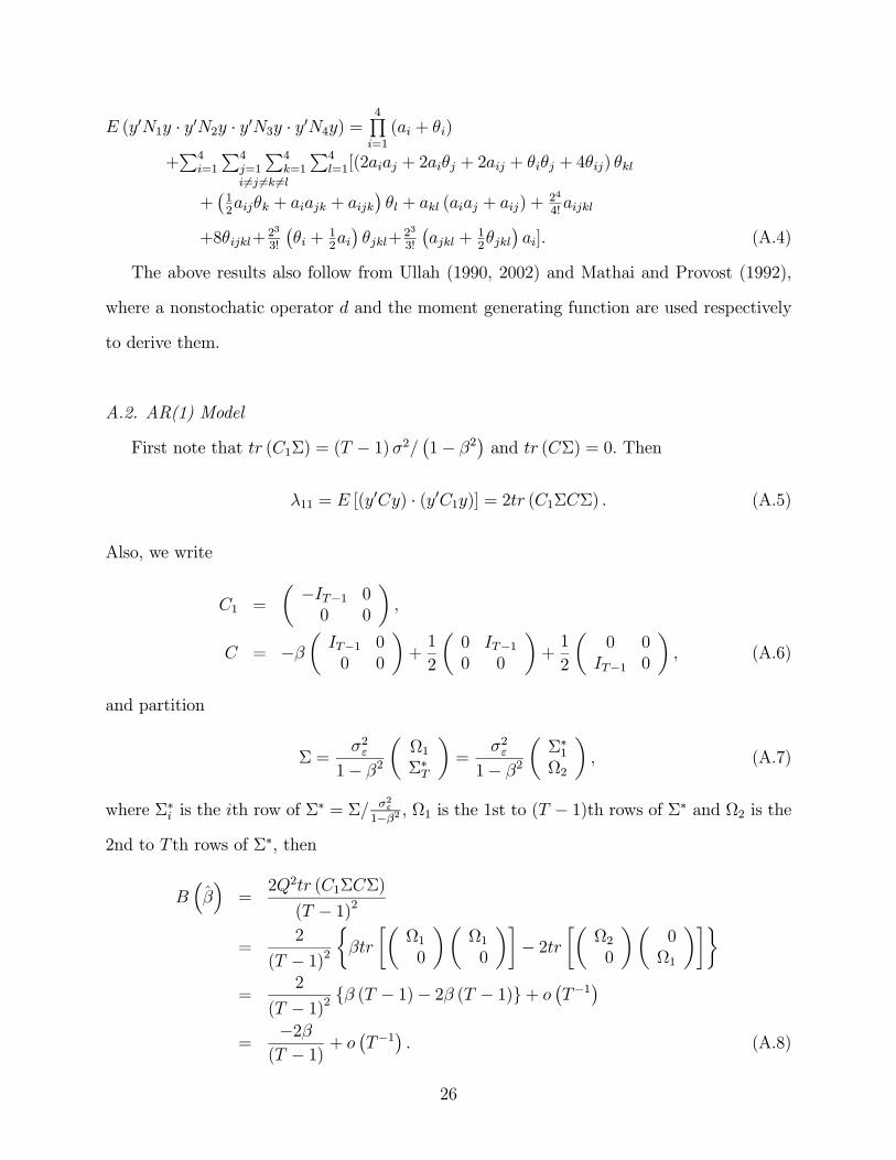
The above results also follow from Ullah (1990, 2002) and Mathai and Provost (1992),

where a nonstochatic operator d and the moment generating function are used respectively

to derive them.

A.2. AR(1) Model

First note that tr (C1Σ) = (T − 1)σ2/¡1− β2

¢and tr (CΣ) = 0. Then

λ11 = E [(y0Cy) · (y0C1y)] = 2tr (C1ΣCΣ) . (A.5)

Also, we write

C1 =

µ −IT−1 00 0

¶,

C = −βµIT−1 00 0

¶+1

2

µ0 IT−10 0

¶+1

2

µ0 0IT−1 0

¶, (A.6)

and partition

Σ =σ2ε

1− β2

µΩ1Σ∗T

¶=

σ2ε1− β2

µΣ∗1Ω2

¶, (A.7)

where Σ∗i is the ith row of Σ∗ = Σ/ σ2ε

1−β2 , Ω1 is the 1st to (T − 1)th rows of Σ∗ and Ω2 is the

2nd to T th rows of Σ∗, then

B³β´=

2Q2tr (C1ΣCΣ)

(T − 1)2

=2

(T − 1)2½βtr

·µΩ10

¶µΩ10

¶¸− 2tr

·µΩ20

¶µ0

Ω1

¶¸¾=

2

(T − 1)2 β (T − 1)− 2β (T − 1)+ o¡T−1

¢=

−2β(T − 1) + o

¡T−1

¢. (A.8)

26

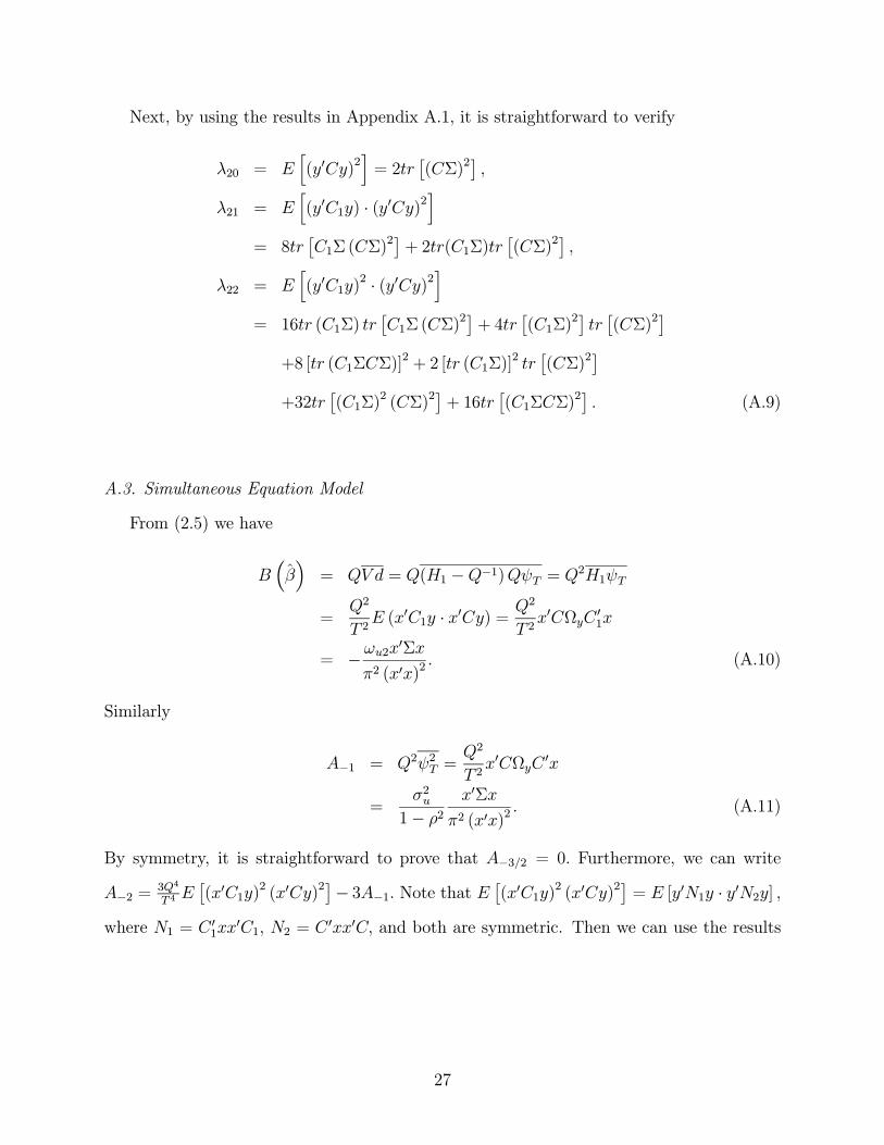
Next, by using the results in Appendix A.1, it is straightforward to verify

λ20 = Eh(y0Cy)2

i= 2tr

£(CΣ)2

¤,

λ21 = Eh(y0C1y) · (y0Cy)2

i= 8tr

£C1Σ (CΣ)

2¤+ 2tr(C1Σ)tr £(CΣ)2¤ ,λ22 = E

h(y0C1y)

2 · (y0Cy)2i

= 16tr (C1Σ) tr£C1Σ (CΣ)

2¤+ 4tr £(C1Σ)2¤ tr £(CΣ)2¤+8 [tr (C1ΣCΣ)]

2 + 2 [tr (C1Σ)]2 tr

£(CΣ)2

¤+32tr

£(C1Σ)

2 (CΣ)2¤+ 16tr

£(C1ΣCΣ)

2¤ . (A.9)

A.3. Simultaneous Equation Model

From (2.5) we have

B³β´= QV d = Q(H1 −Q−1)QψT = Q2H1ψT

=Q2

T 2E (x0C1y · x0Cy) = Q2

T 2x0CΩyC 01x

= −ωu2x0Σx

π2 (x0x)2. (A.10)

Similarly

A−1 = Q2ψ2T =Q2

T 2x0CΩyC 0x

=σ2u

1− ρ2x0Σx

π2 (x0x)2. (A.11)

By symmetry, it is straightforward to prove that A−3/2 = 0. Furthermore, we can write

A−2 =3Q4

T 4E£(x0C1y)

2 (x0Cy)2¤− 3A−1. Note that E £(x0C1y)2 (x0Cy)2¤ = E [y0N1y · y0N2y] ,

where N1 = C01xx

0C1, N2 = C 0xx0C, and both are symmetric. Then we can use the results

27

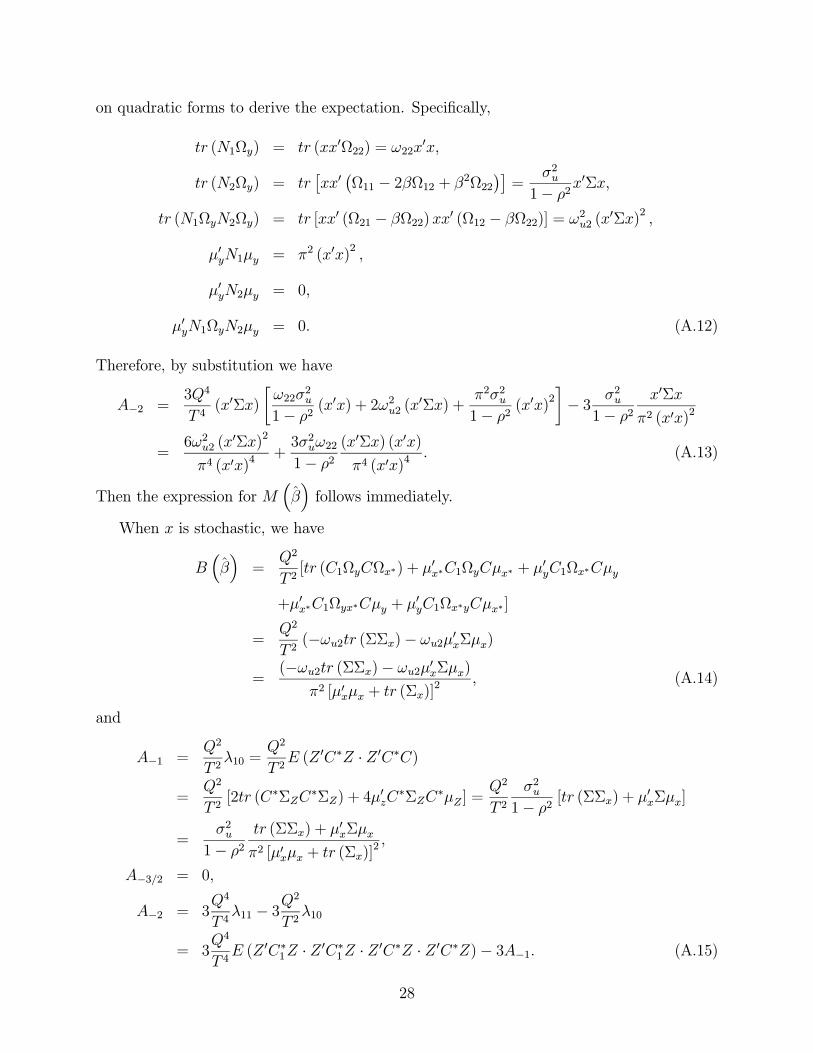
on quadratic forms to derive the expectation. Specifically,

tr (N1Ωy) = tr (xx0Ω22) = ω22x0x,

tr (N2Ωy) = tr£xx0¡Ω11 − 2βΩ12 + β2Ω22

¢¤=

σ2u1− ρ2

x0Σx,

tr (N1ΩyN2Ωy) = tr [xx0 (Ω21 − βΩ22) xx0 (Ω12 − βΩ22)] = ω2u2 (x

0Σx)2 ,

µ0yN1µy = π2 (x0x)2 ,

µ0yN2µy = 0,

µ0yN1ΩyN2µy = 0. (A.12)

Therefore, by substitution we have

A−2 =3Q4

T 4(x0Σx)

·ω22σ

2u

1− ρ2(x0x) + 2ω2u2 (x

0Σx) +π2σ2u1− ρ2

(x0x)2¸− 3 σ2u

1− ρ2x0Σx

π2 (x0x)2

=6ω2u2 (x

0Σx)2

π4 (x0x)4+3σ2uω221− ρ2

(x0Σx) (x0x)

π4 (x0x)4. (A.13)

Then the expression for M³β´follows immediately.

When x is stochastic, we have

B³β´=

Q2

T 2[tr (C1ΩyCΩx∗) + µ

0x∗C1ΩyCµx∗ + µ

0yC1Ωx∗Cµy

+µ0x∗C1Ωyx∗Cµy + µ0yC1Ωx∗yCµx∗]

=Q2

T 2(−ωu2tr (ΣΣx)− ωu2µ

0xΣµx)

=(−ωu2tr (ΣΣx)− ωu2µ

0xΣµx)

π2 [µ0xµx + tr (Σx)]2 , (A.14)

and

A−1 =Q2

T 2λ10 =

Q2

T 2E (Z 0C∗Z · Z 0C∗C)

=Q2

T 2[2tr (C∗ΣZC∗ΣZ) + 4µ0zC

∗ΣZC∗µZ ] =Q2

T 2σ2u

1− ρ2[tr (ΣΣx) + µ

0xΣµx]

=σ2u

1− ρ2tr (ΣΣx) + µ

0xΣµx

π2 [µ0xµx + tr (Σx)]2 ,

A−3/2 = 0,

A−2 = 3Q4

T 4λ11 − 3Q

2

T 2λ10

= 3Q4

T 4E (Z 0C∗1Z · Z 0C∗1Z · Z 0C∗Z · Z 0C∗Z)− 3A−1. (A.15)

28

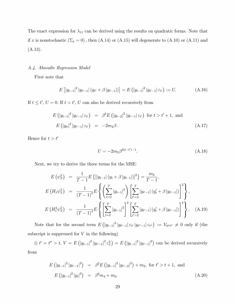
The exact expression for λ11 can be derived using the results on quadratic forms. Note that

if x is nonstochastic (Σx = 0) , then (A.14) or (A.15) will degenerate to (A.10) or (A.11) and

(A.13).

A.4. Absoulte Regression Model

First note that

E£|yt−1|2 |yt0−1| (yt0 + β |yt0−1|)

¤= E

¡|yt−1|2 |yt0−1| εt0¢ := U. (A.16)

If t ≤ t0, U = 0. If t > t0, U can also be derived recursively from

E¡|yt−1|2 |yt0−1| εt0¢ = β2E

¡|yt−2|2 |yt0−1| εt0¢ for t > t0 + 1, andE¡|yt0|2 |yt0−1| εt0¢ = −2m2β. (A.17)

Hence for t > t0

U = −2m2β2(t−t0)−1. (A.18)

Next, we try to derive the three terms for the MSE:

E¡ψ2T¢=

1

T − 1E©[|yt−1| (yt + β |yt−1|)]2

ª=

m2

T − 1 ,

E¡H1ψ

2T

¢=

1

(T − 1)3EÃ

TXt=2

|yt−1|2!"

TXt0=2

|yt0−1| (y0t + β |yt0−1|)#2 ,

E¡H21ψ

2T

¢=

1

(T − 1)4E"

TXt=2

|yt−1|2#2 " TX

t0=2

|yt0−1| (y0t + β |yt0−1|)#2 . (A.19)

Note that for the second term E¡|yt−1|2 |yt0−1| εt0 |yt00−1| εt00¢ := Vtt0t00 6= 0 only if (the

subscript is suppressed for V in the following)

i) t0 = t00 > t, V = E¡|yt−1|2 |yt0−1|2 ε2t0¢ = E ¡|yt−1|2 |yt0−1|2¢ can be derived recursively

from

E¡|yt−1|2 |yt0−1|2¢ = β2E

¡|yt−1|2 |yt0−2|2¢+m2, for t0 > t+ 1, and

E¡|yt−1|2 |yt|2¢ = β2m4 +m2. (A.20)

29

Hence for t0 = t00 > t

V = β2(t0−t)m4 +m2

1− β2(t0−t)

1− β2. (A.21)

ii) t = t0 = t00, V = m4.

iii) t > t0 = t00, V = E¡|yt−1|2 |yt0−1|2 ε2t0¢ can be derived recursively from

E¡|yt−1|2 |yt0−1|2 ε2t0¢ = β2E

¡|yt−2|2 |yt0−1|2 ε2t0¢+m2 for t > t0 + 1, and

E¡|yt0|2 |yt0−1|2 ε2t0¢ = β2m4 + 3m2. (A.22)

Hence for t > t0 = t00

V = β2(t−t0)m4 +m2

1− β2(t−t0−1)

1− β2+ 3m2. (A.23)

iv) t > t0 > t00, V can be derived recursively from

E¡|yt−1|2 |yt0−1| εt0 |yt00−1| εt00¢ = β2E

¡|yt−2|2 |yt0−1| εt0 |yt00−1| εt00¢ for t > t0 + 1, andE¡|yt0|2 |yt0−1| εt0 |yt00−1| εt00¢ = −2βE ¡|yt0−1|2 |yt00−1| εt00¢

= 4m2β2(t0−t00) (substitute (A.18)). (A.24)

Hence for t > t0 > t00

V = 4m2β2(t−t00−1). (A.25)

Also, for the third term E¡|yt−1|2 |yt0−1|2 |yt00−1| εt00 |yt000−1| εt000¢ := Wtt0t00t000 6= 0 only if

(the subscript is suppressed for W in the following)

i) t = t0 = t00 = t000, W = m6

ii) t = t00 = t000 > t0 (or t0 = t00 = t000 > t due to symmetry; the result follows by exchanging

the index t0 with t),W = E¡|yt−1|4 ε2t |yt0−1|2¢ = E ¡|yt−1|4 |yt0−1|2¢ can be derived recursively

from

E¡|yt−1|4 |yt0−1|2¢ = β4E

¡|yt−2|4 |yt0−1|2¢+ 6β2E ¡|yt−2|2 |yt0−1|2¢+ 3m2

= β4E¡|yt−2|4 |yt0−1|2¢+ 6"β2(t−t0)m4 +m2

1− β2(t−t0)

1− β2

#+ 3m2

for t > t0 + 1 (substitute (A.21)), and

E¡|yt0|4 |yt0−1|2¢ = β4m6 + 6β

2m4 + 3m2. (A.26)

30

Hence for t = t00 = t000 > t0

W = β4(t−t0)m6 + 6

"β2(t−t

0)m4 +m21− β2(t−t

0)

1− β2

#1− β2(t−t

0−1)

1− β2

+6β2m4 + 3m21− β4(t−t

0)

1− β4(A.27)

iii) t = t0 > t00 = t000, W = E¡|yt−1|4 |yt00−1|2 ε2t00¢ can be derived recursively from

E¡|yt−1|4 |yt00−1|2 ε2t00¢ = β4E

¡|yt−2|4 |yt00−1|2 ε2t00¢+ 3m2 + 6β2E¡|yt−2|2 |yt00−1|2 ε2t00¢

= β4E¡|yt−2|4 |yt00−1|2 ε2t00¢+ 3m2

+6

"β2(t−t

0)m4 +m21− β2(t−t

0−1)

1− β2+ 3m2

#for t > t00 + 1 (substitute (A.23)), and

E¡|yt00|4 |yt00−1|2 ε2t00¢ = 15m2 + β4m6 + 18β

2m4. (A.28)

Hence for t = t0 > t00 = t000

W = β4(t−t0)m6 + 6

"β2(t−t

0)m4 +m21− β2(t−t

0−1)

1− β2+ 3m2

#1− β2(t−t

0−1)

1− β2

+18β2m4 + 3m21− β4(t−t

0−1)

1− β4+ 15m2. (A.29)

iv) t00 = t000 > t = t0, W = E¡|yt−1|4 |yt00−1|2¢ (note that it is different from ii)) can be

derived recursively from

E¡|yt−1|4 |yt00−1|2¢ = β2E

¡|yt−1|4 |yt00−2|2¢+m4 for t00 > t+ 1, and

E¡|yt−1|4 |yt|2¢ = β2m6 +m4. (A.30)

Hence for t00 = t000 > t = t0

W = β2(t00−t)m6 +m4

1− β2(t00−t)

1− β2(A.31)

31

v) t = t0 > t00 > t000, W = E¡|yt−1|4 |yt00−1| εt00 |yt000−1| εt000¢ can be derived recursively from

E¡|yt−1|4 |yt00−1| εt00 |yt000−1| εt000¢ = β4E

¡|yt−2|4 |yt00−1| εt00 |yt000−1| εt000¢+6β2E

¡|yt−2|2 |yt00−1| εt00 |yt000−1| εt000¢= β4E

¡|yt−2|4 |yt00−1| εt00 |yt000−1| εt000¢+ 24m2β2(t−t000−1)

for t > t00 + 1 (substitute (A.25)), and

E¡|yt00|4 |yt00−1| εt00 |yt000−1| εt000¢ = −4β3E ¡|yt00−1|4 |yt000−1| εt000¢

−12βE ¡|yt00−1|2 |yt000−1| εt000¢ . (A.32)

Apparently, E¡|yt00−1|2 |yt000−1| εt000¢ = −2m2β

2(t00−t000)−1 from (A.18) andE¡|yt00−1|4 |yt000−1| εt000¢

follows a recursion

E¡|yt00−1|4 |yt000−1| εt000¢ = β4E

¡|yt00−2|4 |yt000−1| εt000¢+ 6β2E ¡|yt00−2|2 |yt000−1| εt000¢= β4E

¡|yt00−2|4 |yt000−1| εt000¢− 12m2β2(t00−t000)−1

for t00 > t000 + 1 (substitute (A.18)), and

E¡|yt000|4 |yt000−1| εt000¢ = −4β4m4 − 12βm2. (A.33)

Hence it is straightforward to evaluate W numerically for t = t0 > t00 > t000.

vi) t00 = t000 > t > t0 (or t00 = t000 > t0 > t due to symmetry; the result follows by

exchanging the index t0 with t), W = E¡|yt00−1|2 |yt−1|2 |yt0−1|2¢ follows a recursion

E¡|yt00−1|2 |yt−1|2 |yt0−1|2¢ = β2E

¡|yt00−2|2 |yt−1|2 |yt0−1|2¢+E ¡|yt−1|2 |yt0−1|2¢= β2E

¡|yt00−2|2 |yt−1|2 |yt0−1|2¢+ β2(t−t0)m4 +m2

1− β2(t−t0)

1− β2

for t00 > t+ 1 (substitute (A.21)), and

E¡|yt|2 |yt−1|2 |yt0−1|2¢ = β2E

¡|yt−1|4 |yt0−1|2¢+E ¡|yt−1|2 |yt0−1|2¢= 6β2

"β2(t−t

0)m4 +m21− β2(t−t

0)

1− β2

#1− β2(t−t

0−1)

1− β2

β4(t−t0)+2m6 + 6β

4m4 + 3β2m2

1− β4(t−t0)

1− β4+ β2(t−t

0)m4

+m21− β2(t−t

0)

1− β2(from (A.21) and (A.27)). (A.34)

32

Hence it is straightforward to evaluate W numerically for t00 = t000 > t > t0.

vii) t > t0 > t00 > t000 (or t0 > t > t00 > t000, t > t0 > t000 > t00, t0 > t > t000 > t00; the

results follow by exchanging the indices), W = E¡|yt−1|2 |yt0−1|2 |yt00−1| εt00 |yt000−1| εt000¢ can

be derived recursively from

E¡|yt−1|2 |yt0−1|2 |yt00−1| εt00 |yt000−1| εt000¢ = β2E

¡|yt−2|2 |yt0−1|2 |yt00−1| εt00 |yt000−1| εt000¢+E

¡|yt0−1|2 |yt00−1| εt00 |yt000−1| εt000¢for t > t0 + 1, and

E¡|yt0|2 |yt0−1|2 |yt00−1| εt00 |yt000−1| εt000¢ = β2E

¡|yt0−1|4 |yt00−1| εt00 |yt000−1| εt000¢+E

¡|yt0−1|2 |yt00−1| εt00 |yt000−1| εt000¢ , (A.35)

where E¡|yt0−1|4 |yt00−1| εt00 |yt000−1| εt000¢ follows from v) and E

¡|yt0−1|2 |yt00−1| εt00 |yt000−1| εt000¢follows from (A.25). Hence it is straightforward to evaluate W numerically for t > t0 > t00 >

t000.

Therefore, E¡H1ψ

2T

¢= 1

(T−1)3PPP

Vtt0t00 and E¡H21ψ

2T

¢= 1

(T−1)4PPPP

Wtt0t00t000

can easily be evaluated numerically.

33

References

Amemiya, T., 1980, The n2-order mean squared errors of the maximum likelihood and the

minimum logit chi-square estimators, Annals of Mathematical Statistics 8, 488-505.

Andel, J., I. Netuka and K. Svara, 1984, On threshold autoregressive processes, Kybernetika

20, 89-106.

Anderson, T. W. and T. Sawa, 1973, Distributions of estimator of coeifficients of a single

equation in a simultaneous system and their asymptotic expansions, Econometrica 41,

683-714.

Anderson, T. W. and T. Sawa, 1979, Evaluation of the distribution function of the two-stage

least square estimate, Econometrica 47, 163-182.

Basmann, R. L., 1974, Exact finite sample distribution for some econometric estimators

and test statistics: a survey and appraisal, in: M.D. Intriligator and D. A. Kendrick,

eds., Frontiers of quantitative economics, Vol. 2 (North-Holland, Amsterdam) 209-288.

Brown, T. M., 1952, Habit persistence and lags in consumer behavior, Econometrica 20,

355-371.

Chesher, A. D. and R. Spady, 1989, Asymptotic expansions of the information matrix test

statistic, Econometrica 59, 787-816.

Cordeiro, G. M. and R. Klein, 1994, Bias correction in ARMA models, Statistics and

Probabilities Letters 19, 169-796.

Cordeiro, G. M. and P. McCullagh, 1991, Bias correction in generalized linear models,

Journal of the Royal Statistical Society B 53, 629—643.

Cox, D. R. and J. Snell, 1968, A general definition of residuals, Journal of the Royal

Statistical Society B 30, 248-275.

Engle, R. F., 1982, Autoregressive conditional heteroscedasticity with estimates of the

variance of United Kingdom inflation, Econometrica 50, 987-1007.

Hamilton, J. D., 1994, Time series analysis (Princeton University Press, Princeton).

Iglesias, E. and G. D. A. Phillips, 2001, Small sample properties of ML estimators in AR-

ARCH Models, Mimeo. (Cardiff Business School, Cardiff University, Cardiff, Wales,

UK).

Iglesias, E. and G. D. A. Phillips, 2002, Small sample estimation bias in ARCH Models,

Mimeo. (Cardiff Business School, Cardiff University, Cardiff, Wales, UK).

34

Kiviet, J. F. and Phillips, G. D. A., 1993, Alternative bias approximations in regressions

with a lagged dependent variable, Econometric Theory 9, 62-80.

Koenker, R., J. A. F. Machado, C. L. Skeels, and A. H. Welsh, 1992, Momentary lapses:

moment expansions and the robustness of minimum distance estimation, Mimeo. (Uni-

versity of Illinois, Evanston, IL).

Linton, O., 1997, An asymptotic expansion in the GARCH(1,1) model, Econometric Theory

13, 558-581.

Lovell, M. C., 1961, Manufacturers’ inventories, sales expectations and the acceleration

principle, Econometrica 29, 293-314.

Magnus, J. R., 1978, The moments of products of quadratic forms in normal variables,

Statistica Neerlandica 32, 201-210.

Magnus, J. R., 1979, The expectation of products of quadratic forms in normal variables:

the practice, Statistica Neerlandica 33, 131-136.

Mathai, A. M. and S. B. Provost, 1992, Quadratic forms in random variables (Marcel

Dekker, New York).

Nagar, A. L., 1959, The bias and moment matrix of the general k-class estimators of the

parameters in simultaneous equations, Econometrica 27, 575-595.

Newey, W. K. and R. J. Smith, 2001, Higher order properties of GMM and generalized

empirical likelihood estimators, Working paper. (MIT and University of Bristol).

Phillips, P. C. B., 1977, Approximations to some finite sample distributions associated with

a first-order stochastic difference equations, Econometrica 45, 463-485.

Phillips, P. C. B., 1987, Asymptotic expansions in nonstationary vector autoregression,

Econometric Theory 3, 45-68.

Rilstone, P., V. K. Srivastara, and A. Ullah, 1996, The second-order bias and mean squared

error of nonlinear estimators, Journal of Econometrics 75, 369-385.

Roberston, C. A. and J. G. Fryer, 1970, The bias and accuracy of moment estimators,

Biometrika 57, 57-65.

Rothenberg, T. J., 1984, Approximating the distribution of econometric estimators and test

statistics, in: M. L. Intriligator and Z. Griliches, eds., Handbook of econometrics, Vol.

2, (North-Holland, Amsterdam).

Sargan, J. D., 1974, The validity of Nagar’s expansion for the moments of econometric

estimators, Econometrica 42, 169-176.

35

Sargan, J. D., 1976, Econometric estimators and the Edgeworth approximations, Econo-

metrica 44, 421-448.

Tong, H., 1990, Non-linear time series: a dynamical system approcah (Oxford University

Press, New York).

Ullah, A., 1990, Finite sample econometrics: a unified approach, in: R. A. L. Carter, J.

Dutta and A. Ullah, eds., Contributions to econometric theory and application, Volume

in honor of A. L. Nagar (Springer-Verlag, New York).

Ullah, A. and V. K. Srivastava, 1994, Moments of the ratio of quadratic forms in non-normal

variables with econometric examples, Journal of Econometrics 62, 129-141.

Ullah, A., 2002, Finite sample econometrics, Manuscript. (Department of Economics, Uni-

versity of California, Riverside).

36

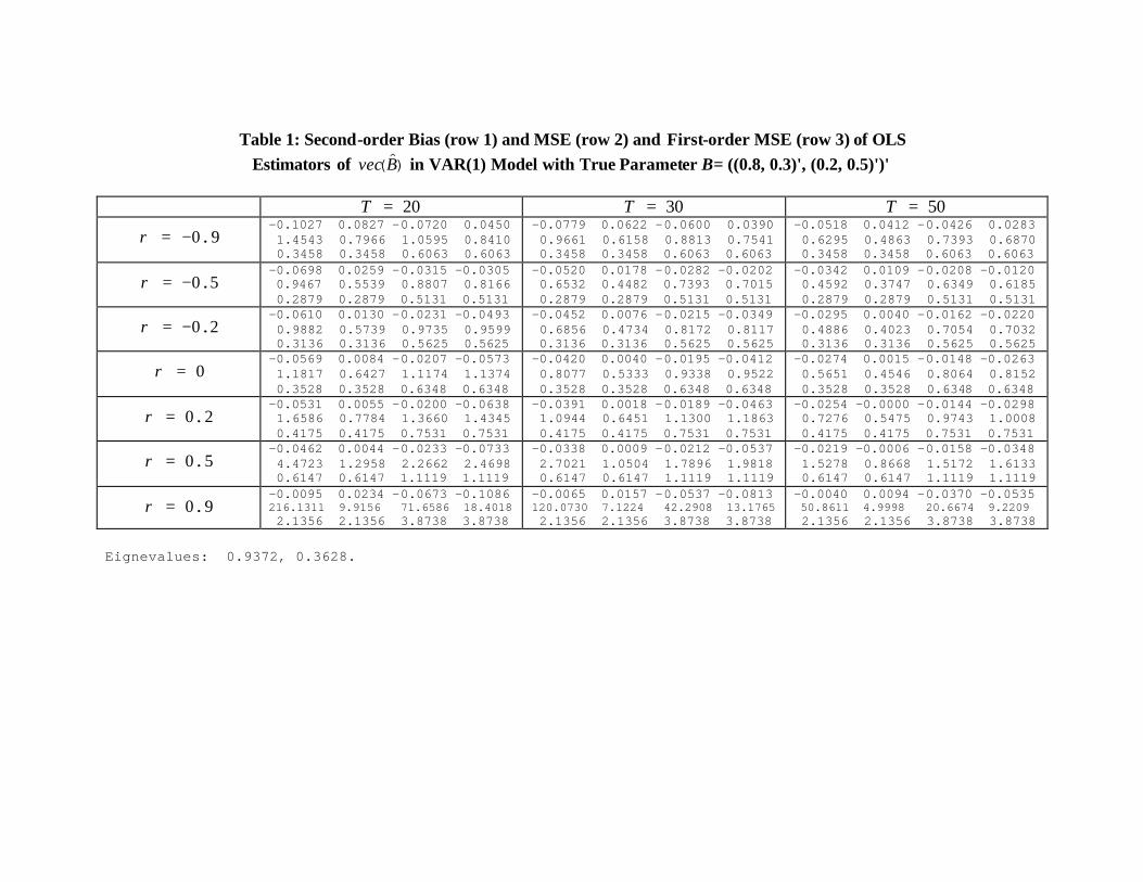
Table 1: Second-order Bias (row 1) and MSE (row 2) and First-order MSE (row 3) of OLS Estimators of )(Bvec in VAR(1) Model with True Parameter B= ((0.8, 0.3)', (0.2, 0.5)')'

20=T 30=T 50=T

90.−=ρ -0.1027 0.0827 -0.0720 0.0450 1.4543 0.7966 1.0595 0.8410 0.3458 0.3458 0.6063 0.6063

-0.0779 0.0622 -0.0600 0.0390 0.9661 0.6158 0.8813 0.7541 0.3458 0.3458 0.6063 0.6063

-0.0518 0.0412 -0.0426 0.0283 0.6295 0.4863 0.7393 0.6870 0.3458 0.3458 0.6063 0.6063

50.−=ρ -0.0698 0.0259 -0.0315 -0.0305 0.9467 0.5539 0.8807 0.8166 0.2879 0.2879 0.5131 0.5131

-0.0520 0.0178 -0.0282 -0.0202 0.6532 0.4482 0.7393 0.7015 0.2879 0.2879 0.5131 0.5131

-0.0342 0.0109 -0.0208 -0.0120 0.4592 0.3747 0.6349 0.6185 0.2879 0.2879 0.5131 0.5131

20.−=ρ -0.0610 0.0130 -0.0231 -0.0493 0.9882 0.5739 0.9735 0.9599 0.3136 0.3136 0.5625 0.5625

-0.0452 0.0076 -0.0215 -0.0349 0.6856 0.4734 0.8172 0.8117 0.3136 0.3136 0.5625 0.5625

-0.0295 0.0040 -0.0162 -0.0220 0.4886 0.4023 0.7054 0.7032 0.3136 0.3136 0.5625 0.5625

0=ρ -0.0569 0.0084 -0.0207 -0.0573 1.1817 0.6427 1.1174 1.1374 0.3528 0.3528 0.6348 0.6348

-0.0420 0.0040 -0.0195 -0.0412 0.8077 0.5333 0.9338 0.9522 0.3528 0.3528 0.6348 0.6348

-0.0274 0.0015 -0.0148 -0.0263 0.5651 0.4546 0.8064 0.8152 0.3528 0.3528 0.6348 0.6348

20.=ρ -0.0531 0.0055 -0.0200 -0.0638 1.6586 0.7784 1.3660 1.4345 0.4175 0.4175 0.7531 0.7531

-0.0391 0.0018 -0.0189 -0.0463 1.0944 0.6451 1.1300 1.1863 0.4175 0.4175 0.7531 0.7531

-0.0254 -0.0000 -0.0144 -0.0298 0.7276 0.5475 0.9743 1.0008 0.4175 0.4175 0.7531 0.7531

50.=ρ -0.0462 0.0044 -0.0233 -0.0733 4.4723 1.2958 2.2662 2.4698 0.6147 0.6147 1.1119 1.1119

-0.0338 0.0009 -0.0212 -0.0537 2.7021 1.0504 1.7896 1.9818 0.6147 0.6147 1.1119 1.1119

-0.0219 -0.0006 -0.0158 -0.0348 1.5278 0.8668 1.5172 1.6133 0.6147 0.6147 1.1119 1.1119

90.=ρ -0.0095 0.0234 -0.0673 -0.1086 216.1311 9.9156 71.6586 18.4018 2.1356 2.1356 3.8738 3.8738

-0.0065 0.0157 -0.0537 -0.0813 120.0730 7.1224 42.2908 13.1765 2.1356 2.1356 3.8738 3.8738

-0.0040 0.0094 -0.0370 -0.0535 50.8611 4.9998 20.6674 9.2209 2.1356 2.1356 3.8738 3.8738

Eignevalues: 0.9372, 0.3628.

Table 1 (Continued): Second-order Bias (row 1) and MSE (row 2) and First-order MSE (row 3) of OLS Estimators of )(Bvec in VAR(1) Model with True Parameter B = ((0.1, 0.4)', (0.4, 0.3)')'

20=T 30=T 50=T

90.−=ρ -0.0235 -0.0210 -0.0285 -0.0181 7.9322 / / / 2.9278 2.9278 3.0711 3.0711

-0.0152 -0.0149 -0.0186 -0.0130 5.4407 0.8221 / / 2.9278 2.9278 3.0711 3.0711

-0.0089 -0.0093 -0.0109 -0.0082 4.0841 1.6959 0.6082 0.7966 2.9278 2.9278 3.0711 3.0711

50.−=ρ -0.0230 -0.0259 -0.0291 -0.0243 1.9363 1.6420 1.0409 1.0338 0.9490 0.9490 0.9247 0.9247

-0.0155 -0.0176 -0.0196 -0.0166 1.5348 1.3804 0.9881 0.9864 0.9490 0.9490 0.9247 0.9247

-0.0093 -0.0107 -0.0118 -0.0101 1.2683 1.1936 0.9566 0.9564 0.9490 0.9490 0.9247 0.9247

20.−=ρ -0.0223 -0.0257 -0.0298 -0.0256 1.7294 1.4596 1.0303 1.0170 0.8174 0.8174 0.7598 0.7598

-0.0151 -0.0175 -0.0201 -0.0174 1.3634 1.2200 0.9212 0.9167 0.8174 0.8174 0.7598 0.7598

-0.0091 -0.0106 -0.0121 -0.0106 1.1173 1.0470 0.8482 0.8469 0.8174 0.8174 0.7598 0.7598

0=ρ -0.0216 -0.0252 -0.0304 -0.0264 1.7272 1.4613 1.0691 1.0532 0.8300 0.8300 0.7500 0.7500

-0.0146 -0.0171 -0.0205 -0.0179 1.3683 1.2271 0.9426 0.9369 0.8300 0.8300 0.7500 0.7500

-0.0089 -0.0104 -0.0124 -0.0109 1.1262 1.0572 0.8565 0.8548 0.8300 0.8300 0.7500 0.7500

20.=ρ -0.0206 -0.0243 -0.0313 -0.0275 1.8326 1.5613 1.1725 1.1512 0.9096 0.9096 0.8007 0.8007

-0.0139 -0.0165 -0.0211 -0.0186 1.4642 1.3208 1.0268 1.0186 0.9096 0.9096 0.8007 0.8007

-0.0085 -0.0100 -0.0128 -0.0113 1.2151 1.1455 0.9265 0.9239 0.9096 0.9096 0.8007 0.8007

50.=ρ -0.0175 -0.0213 -0.0341 -0.0305 2.3308 2.0199 1.5644 1.5219 1.2414 1.2414 1.0546 1.0546

-0.0119 -0.0145 -0.0230 -0.0206 1.8963 1.7351 1.3666 1.3492 1.2414 1.2414 1.0546 1.0546

-0.0072 -0.0088 -0.0139 -0.0125 1.6026 1.5260 1.2292 1.2233 1.2414 1.2414 1.0546 1.0546

90.=ρ 0.0115 0.0081 -0.0602 -0.0571 7.1723 6.2716 4.8100 4.7357 4.7797 4.7797 3.8935 3.8935

0.0074 0.0051 -0.0404 -0.0383 6.1245 5.7231 4.4899 4.4397 4.7797 4.7797 3.8935 3.8935

0.0044 0.0029 -0.0243 -0.0231 5.4763 5.3228 4.2380 4.2146 4.7797 4.7797 3.8935 3.8935

Eignevalues: -0.2123, 0.6123.