Linear Time Euclidean Distance TransformAlgorithmsHeinz Breu Joseph Gil David KirkpatrickMichael WermanAbstractTwo linear time (and hence asymptotically optimal) algorithms forcomputing the Euclidean distance transform of a two-dimensional bi-nary image are presented. The algorithms are based on the constructionand regular sampling of the Voronoi diagram whose sites consist of theunit (feature) pixels in the image. The �rst algorithm, which is of pri-marily theoretical interest, constructs the complete Voronoi diagram.The second, more practical, algorithm constructs the Voronoi diagramwhere it intersects the horizontal lines passing through the image pixelcentres. Extensions to higher dimensional images and to other distancefunctions are also discussed.1 IntroductionA two-dimensional binary image is a function, I, from the elements of ann by m array, referred to as pixels, to f0; 1g. Pixels of unit (respectively,zero) value are referred to as feature (respectively, background) pixels of theimage. We associate the pixel in row r and column c with the Cartesian point(c; r). Thus, any distance function de�ned on the Cartesian plane induces adistance function on the space of image pixels. For a given distance function,the distance transform of an image I is an assignment, to each pixel p, of thedistance between p and the closest feature pixel in I. The nearest-neighbourtransform of an image is an assignment, to each pixel p, of the identity (ordistance information su�cient to compute the identity in O(1) time) of afeature pixel closest to p. Assuming that computing the distance between twopixels is a O(1) time operation, it should be clear that the distance transformcan be constructed from the nearest-neighbour transform in time linear in thetotal number of pixels. It should also be clear that, at least in their explicitforms, both transforms require at least linear time for their computation.1

Distance and nearest-neighbour transforms have for a considerable timebeen recognized as important sources and encodings of metric information as-sociated with images in digital picture processing, pattern recognition, roboticsand related applications [17, 13, 2, 1, 10, 6, 11]. Such transforms were �rstintroduced by Rosenfeld and Pfaltz [18, 19] and have been the focus of anextensive literature (cf. [13, 16]).The most natural metric for computing distance in most applications isthe Euclidean metric. However, the lack of e�cient algorithms for computingthe Euclidean distance transform has led many researchers to de�ne and useother metrics (such as city-block, chessboard or chamfer [8, 22, 4]), or approx-imations to the exact Euclidean distance transform [7, 4, 5, 22]. While othermetrics lend themselves to e�cient algorithms, they do so at the expense ofbeing dependent on the orientation of the coordinate system used for repre-senting the image. To quote Borgefors [4], \If the Euclidean distance transformcould be easily computed there would be no need for approximations".By its de�nition, the Euclidean distance transform is a global operation;the most straightforward approach to its construction involves, for each pixel,an amount of computation that is proportional to the size of the entire image(O(nm)). In practice, one hopes to exploit the fact that the distance transformis a discretized version of the continuous distance transform associated with thefeature pixels. Speci�cally, the transform values in a neighbourhood vary ina smooth and predictable fashion. Non-trivial approaches to the constructionof (approximate) Euclidean distance transforms involve the propagation ofdistance information from pixels to neighbouring pixels. Methods vary onthe size and shape of the neighbourhood, and the order in which pixels areprocessed.In one family of algorithms (cf. [4, 7]), each pixel p consults, perhaps re-peatedly, with other pixels in a typically small neighbourhood of p, and basesits updated transform value on those of its neighbours. A tradeo� exists be-tween the quality of the resulting approximation, the size and shape of theneighbourhood, and the number of iterations performed. The total computa-tional e�ort is proportional to the number of pixels, the neighbourhood size,and the number of iterations. Thus, to minimize cost, sequential algorithmstypically use a constant (independent of the image size) sized neighbourhoodand a constant number of iterations often structured to process pixels in somekind of scan order. Parallel implementations of this approach (cf. [21]) repeat-edly update the transform value until it stabilizes (i.e., until a parallel roundbrings no change). In the worst case this may involve a number of iterationsproportional to the image perimeter (O(maxfn;mg)), but this is o�set by thefact that individual pixels are processed in parallel.Danielsson [7] describes a sequential nearest-neighbour transform algorithm2

of the above type, and shows that it is accurate to within one pixel, that is, theidenti�ed neighbour may be up to one pixel further away than the true nearestneighbour. Danielsson also argues that errors of this magnitude are inevitablewith algorithms of this type (due essentially to discontinuities arising fromthe discretization of the continuous nearest-neighbour transform). Yamada[21] shows that parallel implementations are not subject to the same inher-ent approximation errors. Yamada proves that with a suitably large (in fact,eight element) neighbourhood, one can exploit the di�erence between propa-gation distance and Euclidean distance to overcome the problems arising fromdiscretization. Thus, we have inexact sequential algorithms that take O(nm)time in the worst case, or exact parallel algorithms that take O(maxfn;mg)parallel time with O(nm) processors.An alternative approach that does not lend itself as readily to parallelimplementation, involves simulating a wavefront emanating from all featurepixels (cf. [16] and references therein). The idea here is to have certain pixels(those on the current wavefront) inform their neighbours so that the lattercan update their distance transform values, and possibly join the wavefront.Thus, at any moment the propagation of distance information takes placeonly where there is potential for change. Algorithms of this type di�er in theirstrategies for updating the wavefront. In fact, the scan-based algorithms canbe viewed as a kind of wavefront approach as well. The wavefront approachsu�ers from the same inherent discretization error discussed above. Despitethis, Ragnemalm [16] claims that it is possible to simulate Yamada's error-freealgorithm using an O(nm) time sequential wavefront algorithm. However, noproof of this assertion is provided (other than experimental \veri�cation").Yet another approach, again pioneered by Rosenfeld and Pfaltz [18], isbased on the idea of dimensionality reduction. In short, the transform is �rstconstructed using the distance function in one lower dimension (say, restrictedto the pixels in a given row of the image) and then this intermediate resultis used in a second phase to construct the full two-dimensional transform.Paglieroni [14, 13] abstracts this approach, showing that it is applicable toa broad class of distance functions, including Euclidean distance. While cer-tain heuristics apply, even in the most abstract setting, to reduce the cost ontypical images, the worst-case cost for an n by m image is �(nmminfn;mg).Recently an O(nm log(nm)) time algorithm for computing the exact Euclideandistance transform was proposed [12]. This algorithm can be viewed as a spe-cial instance of Paglieroni's algorithm, in which properties of the Euclideanmetric are exploited. The algorithm presented in Section 3 of this paper couldbe interpreted as a further (and, in an asymptotic sense, ultimate) re�nementof Paglieroni's algorithm for Euclidean distance transforms.In the next two sections of this paper two linear (in the size of the im-3

age) time algorithms for constructing the nearest-neighbour transform are de-scribed. Both algorithms are based on the construction of the Voronoi diagramwhose sites are the feature pixels. The �rst algorithm, which is of primarilytheoretical interest, constructs the complete Voronoi diagram. The second,more practical, algorithm constructs the Voronoi diagram where it intersectsthe horizontal lines passing through the image pixel centres. The Voronoi dia-gram [20, 9] of a set of sites S = fh1; : : : ; hsg, denoted VS, consists of s disjointVoronoi cells fCSh1 ; : : : ; CShsg, where CSh (or simply Ch, if S is understood) de-notes the set of all points in the plane whose closest site is h, together with thecell boundaries formed by points equidistant from two (Voronoi edge points)or more (Voronoi vertices) sites. We refer to h as the Voronoi centre of CSh .The nearest-neighbour transform can be viewed as a discretized version ofthe Voronoi diagram, formed by sampling the diagram (i.e. recording the asso-ciated Voronoi centres) at points corresponding to all pixel locations. Despitethis, our algorithms �rst view the problem in its continuous form ignoring(at least for the sake of the algorithm design) the inherent discreteness andregularity of the inputs and outputs. It would appear that the willingness toaddress the problem in its continuous form is the key to developing simple andasymptotically optimal algorithms for the Euclidean distance transform. Wenote, however, that the discreteness and regularity of the inputs and outputsdo play an essential role in the detailed design of the algorithms, and in theiranalysis. In fact, it is well known (cf. [15]) that linear algorithms do not existfor determining, for each of an arbitrary set of query points, the closest of anarbitrary collection of sites.2 Transform based on Complete Voronoi Di-agram ConstructionDetermining the nearest among s arbitrary sites for each of q arbitrary querypoints requires, in the worst case, �(s log s) time to construct the Voronoidiagram of the sites and �(q log s) time to answer the queries (even if thediagram is given). In fact, these bounds are realized by familiar algorithmsfor constructing and querying Voronoi diagrams (cf. [15]). For our applicationthis gives an immediate O(nm log(nm)) time nearest-neighbour transform al-gorithm, since the number of pixels (and hence the number of both sites andquery points) is O(nm). Our objective, in the remainder of this section, is todemonstrate that this time complexity can be reduced to O(nm) by exploitingthe fact that both sites and query points are subsets of a two-dimensional pixelarray. 4

2.1 Voronoi diagrams of pixel subsetsA familiar approach (cf. [15]) to the construction of Voronoi diagrams isdivide and conquer: (linearly) separate the sites into two subsets, recursivelyconstruct the Voronoi diagrams of the subsets, and \merge" the resultingdiagrams into the Voronoi diagram of the full set. The linear separation of thesubsets ensures that much of the structure of the smaller Voronoi diagrams canbe retained; they are in e�ect \sewn together" along one (monotone) chain ofedges (called the Voronoi merge boundary) formed by points with two nearestsites, one from each subset. The cost of the merge step is proportional to thenumber of edges on this chain, which is just the number of cells that borderon this chain. While the latter may be signi�cantly larger than the number ofcells that intersect the partition boundary (the line separating the set of sites),it is, of course, at worst the total number of sites, s. Thus if each separation isbalanced the depth of the recursion is O(log s) and the total cost is O(s log s).If we take note of the fact that (i) the sites consist of a subset of some nby m array of pixels and (ii) it su�ces to construct the Voronoi diagram re-stricted to the rectangle [1; n]� [1;m], then we can ignore the structure of thesubset and partition the array instead (by splitting it in half along its longestdimension). Although this may lead to an unbalanced division of the sitesthemselves, it is not di�cult to show that the cost of merging the Voronoi di-agrams of the resulting site subsets is sublinear in the size of the participatingarrays, which gives rise to a linear total cost. (Intuitively, if a site is far re-moved from the partition boundary or if it is surrounded by other closer sites,its cell cannot border the Voronoi merge boundary. More precisely, if a sitein any i by j subproblem has distance greater than minfn;mg from the parti-tion boundary then it cannot in uence the Voronoi merge boundary for thatsubproblem. Furthermore, if a site has distance greater than (minfi; jg)1=2from the boundary of its subarray, then it can in uence the merge boundaryonly if at least one of its four rectilinear closest sites has distance at least(minfi; jg)1=2.) Thus, if T (i; j) denotes the worse-case cost of constructing theVoronoi diagram for any set of sites drawn from an i by j subarray of an nby m array, we have the recurrences T (n; 2kn) � 2T (n; 2k�1n) + O(n2), sincethere are O(n2) pixels of distance at most n from the partition boundary oftwo n by 2k�1n subarrays, and T (i; i) � 4T (i=2; i=2) +O(i3=2), since there areO(i3=2) pixels of distance at most i1=2 from the boundary of an i by i array, andat most O(i3=2) of the remaining sites can in uence the merge boundary, bythe sparsity condition. If follows from these recurrences that T (n; n) = O(n2)and, more generally, T (n;m) = O(nm).5

2.2 Finding nearest pixels given the Voronoi diagramGiven the Voronoi diagram of the feature pixels, we can �nd the feature pixelnearest to pixel p by determining the Voronoi cell containing p. If we treat allsuch queries independently there is no way to avoid taking (nm log(nm)) timein the worst case. However, it we batch the queries into rows then all O(nm)queries can be answered in O(nm) time in total. This follows from the factsthat (i) a Voronoi diagram on s sites can be decomposed, in O(s) time, intotrapezoids whose non-horizontal edges are portions of Voronoi edges; (ii) thecost of visiting, in sequence, all of the Voronoi cells (equivalently, trapezoids)intersected by a horizontal line is proportional to the number of cells visited;and (iii) any horizontal line intersects the Voronoi diagram of a set of sitesdrawn from an n by m array in O(m) cells (at most two cells are associatedwith sites in any �xed column).2.3 Advantages and drawbacksThe nearest-neighbour transform algorithm implicit in the preceding subsec-tions has several attractive features in addition to its asymptotically optimalworst case complexity. First, we note that it can be implemented using ex-act rational arithmetic, since it is concerned exclusively with bisectors of pixelpairs. Second, it seems to be more adaptable than most array-based algorithmsto sparse images (assuming the feature pixels can be succinctly speci�ed) andto the computation of \partial" nearest-neighbour transforms (i.e. computa-tion of transform values at only a small subset of the domain). In both ofthese cases, the analysis above may be unduly pessimistic.On the other hand, this explicit Voronoi diagram construction requiresextra space of size proportional to the input image. In addition this spacemust be used to represent a data structure whose complexity far exceeds thatof the input or output of the problem. The latter has an impact not only onthe constants of proportionality inherent in any implementation, but also onthe extent to which the algorithm can be e�ectively parallelized.In the next section, we develop another asymptotically optimal nearest-neighbour transform algorithm that retains the advantages of the explicitVoronoi diagram approach along with the simpler data structures of the ear-lier array-based algorithms. This is achieved by constructing only a partialVoronoi diagram, that is, determining its structure only where it is necessaryto know it. 6

3 Transform based on Partial Voronoi Dia-gram ConstructionThe nearest-neighbour transform is a discretized representation of the Voronoidiagram of the feature pixels of a given image. In the previous section wedemonstrated that the transform can be computed e�ciently by �rst con-structing the (complete) Voronoi diagram and then sampling it at all pixel lo-cations. In this section we show that we can achieve the same asymptotic timecomplexity, together with signi�cant practical improvements, by constructinga Voronoi structure intermediate between the complete Voronoi diagram andthe discretized version that is our ultimate objective. Speci�cally, we constructdirectly the intersection of the Voronoi diagram of the feature pixels with eachrow of the image. Since each such construct has complexity bounded by thewidth of the image, and each row can be processed independently, the totalamount of auxiliary space is signi�cantly reduced (compared to the previous al-gorithm) and the potential for exploiting parallelism is signi�cantly increased.3.1 High level descriptionAs before, the algorithm takes as input an n by m binary image I. Let Fdenote the set of feature pixels of I, let F r denote the set F restricted torows 1 through r, and let Vr denote the Voronoi diagram of F r. For each rowr, the algorithm computes the intersection of Vr with row r. More precisely,at its rth iteration the algorithm constructs the list Lr of Voronoi cells in Vrthat intersect the line y = r (which we denote by Rr). Note that Lr can beconveniently represented as a list of Voronoi centres (pixels) sorted by columnorder.If p and q are distinct points in the plane, we denote by cpq the intersectionof the perpendicular bisector between p and q with the line Rr. If p is anypoint in the plane, we denote its coordinates by (p:x; p:y). (For the sake ofconsistency, imagine that the rows of an image are numbered from bottom totop, and the columns are numbered from left to right.)Observation 1 If u and v belong to F r, and u:x = v:x and u:y > v:y, thenthe Voronoi cell centred at site v in Vr (i.e. CFrv ) does not intersect Rr.Observation 2 If u and v belong to F r, and u:x < v:x, then CF ru (respec-tively, CF rv ) lies to the left (respectively, right) of the perpendicular bisectorbetween u and v. 7

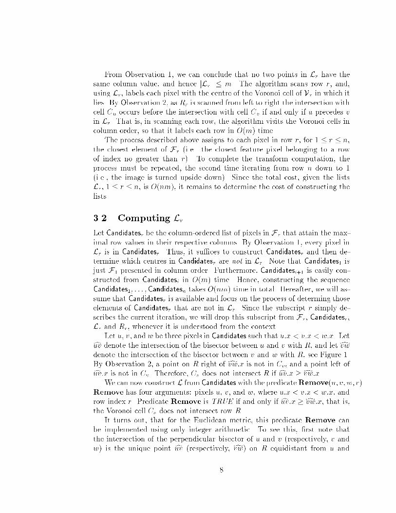
From Observation 1, we can conclude that no two points in Lr have thesame column value, and hence jLrj � m. The algorithm scans row r, and,using Lr, labels each pixel with the centre of the Voronoi cell of Vr in which itlies. By Observation 2, as Rr is scanned from left to right the intersection withcell Cu occurs before the intersection with cell Cv if and only if u precedes vin Lr. That is, in scanning each row, the algorithm visits the Voronoi cells incolumn order, so that it labels each row in O(m) time.The process described above assigns to each pixel in row r, for 1 � r � n,the closest element of F r (i.e. the closest feature pixel belonging to a rowof index no greater than r). To complete the transform computation, theprocess must be repeated, the second time iterating from row n down to 1(i.e., the image is turned upside down). Since the total cost, given the listsLr, 1 � r � n, is O(nm), it remains to determine the cost of constructing thelists.3.2 Computing LrLet Candidatesr be the column-ordered list of pixels in F r that attain the max-imal row values in their respective columns. By Observation 1, every pixel inLr is in Candidatesr. Thus, it su�ces to construct Candidatesr and then de-termine which centres in Candidatesr are not in Lr. Note that Candidates1 isjust F1 presented in column order. Furthermore, Candidatesi+1 is easily con-structed from Candidatesi in O(m) time. Hence, constructing the sequenceCandidates1; : : : ;Candidatesn takes O(nm) time in total. Hereafter, we will as-sume that Candidatesr is available and focus on the process of determing thoseelements of Candidatesr that are not in Lr. Since the subscript r simply de-scribes the current iteration, we will drop this subscript from Fr, Candidatesr,Lr and Rr, whenever it is understood from the context.Let u, v, and w be three pixels in Candidates such that u:x < v:x < w:x. Letcuv denote the intersection of the bisector between u and v with R, and letdvwdenote the intersection of the bisector between v and w with R, see Figure 1.By Observation 2, a point on R right of dvw:x is not in Cv, and a point left ofcuv:x is not in Cv. Therefore, Cv does not intersect R if cuv:x �dvw:x.We can now construct L from Candidates with the predicateRemove(u; v; w; r).Remove has four arguments: pixels u, v, and w, where u:x < v:x < w:x, androw index r. Predicate Remove is TRUE if and only if cuv:x �dvw:x, that is,the Voronoi cell Cv does not intersect row R.It turns out, that for the Euclidean metric, this predicate Remove canbe implemented using only integer arithmetic. To see this, �rst note thatthe intersection of the perpendicular bisector of u and v (respectively, v andw) is the unique point cuv (respectively, dvw) on R equidistant from u and8

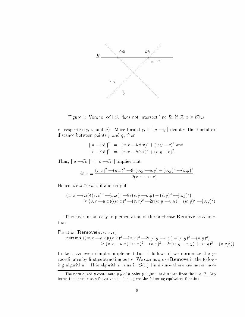
u v wdvw cuvRr c c cc c@@@@@@@@@@@@@@��������������

Figure 1: Voronoi cell Cv does not intersect line Rr if cuv:x �dvw:x.v (respectively, u and v). More formally, if jjp � qjj denotes the Euclideandistance between points p and q, thenjju� cuvjj2 = (u:x� cuv:x)2 + (u:y � r)2 andjjv � cuvjj2 = (v:x� cuv:x)2 + (v:y� r)2:Thus, jju� cuvjj = jjv � cuvjj implies thatcuv:x = (v:x)2� (u:x)2 � 2r(v:y � u:y) + (v:y)2� (u:y)22(v:x� u:x) :Hence, cuv:x �dvw:x if and only if(w:x� v:x)((v:x)2� (u:x)2 � 2r(v:y � u:y) + (v:y)2� (u:y)2)� (v:x� u:x)((w:x)2� (v:x)2 � 2r(w:y � v:y) + (w:y)2 � (v:y)2).This gives us an easy implementation of the predicate Remove as a func-tion.Function Remove(u; v; w; r)return ((w:x� v:x)((v:x)2� (u:x)2 � 2r(v:y � u:y) + (v:y)2� (u:y)2)� (v:x� u:x)((w:x)2� (v:x)2� 2r(w:y � v:y) + (w:y)2 � (v:y)2))In fact, an even simpler implementation 1 follows if we normalize the y-coordinates by �rst subtracting out r. We can now use Remove in the follow-ing algorithm. This algorithm runs in O(n) time since there are never more1The normalized y-coordinate p:�y of a point p is just its distance from the line R. Anyterms that have r as a factor vanish. This gives the following equivalent function.9

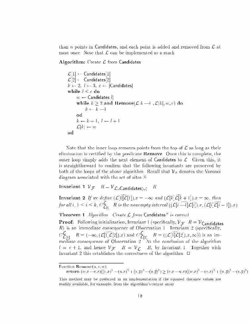
than n points in Candidates, and each point is added and removed from L atmost once. Note that L can be implemented as a stack.Algorithm: Create L from Candidates.L[1] Candidates[1]L[2] Candidates[2]k 2; l 3; c jCandidatesjwhile l � c dow Candidates[l]while k � 2 and Remove(L[k � 1];L[k]; w; r) dok k � 1odk k + 1; l l+ 1L[k] wodNote that the inner loop removes points from the top of L as long as theirelimination is certi�ed by the predicate Remove. Once this is complete, theouter loop simply adds the next element of Candidates to L. Given this, itis straightforward to con�rm that the following invariants are preserved byboth of the loops of the above algorithm. Recall that VS denotes the Voronoidiagram associated with the set of sites S.Invariant 1 VF \R = VL[Candidates[l;c] \R.Invariant 2 If we de�ne ( dL[0]L[1]):x = �1 and ( dL[k]L[k + 1]):x =1, thenfor all i, 1 � i � k, CLL[i]\R is the nonempty interval (( dL[i� 1]L[i]):x; ( dL[i]L[i+ 1]):x).Theorem 1 Algorithm \Create L from Candidates" is correct.Proof: Following initialization, Invariant 1 (speci�cally, VF\R = VCandidates\R) is an immediate consequence of Observation 1. Invariant 2 (speci�cally,CLL[1] \ R = (�1; ( dL[1]L[2]):x) and CLL[2] \ R = (( dL[1]L[2]):x;1)) is an im-mediate consequence of Observation 2. At the conclusion of the algorithml = c + 1, and hence VF \ R = VL \ R, by Invariant 1. Together withInvariant 2 this establishes the correctness of the algorithm. 2Function Remove(u; v; w)return (w:x� v:x)((v:x)2 � (u:x)2 + (v:�y)2 � (u:�y)2) � (v:x� u:x)((w:x)2� (v:x)2 + (w:�y)2 � (v:�y)2)This method may be preferred in an implementation if the squared distance values arereadily available, for example, from the algorithm's output array.10

4 ConclusionsWe have presented two linear-time algorithms for constructing the nearest-neighbour (or distance) transform of a two-dimensional binary image underthe Euclidean metric. Apparently, these are the �rst such algorithms whoseworst case optimality has been formally veri�ed. Interestingly, the algorithmsare conceptually simple enough that they are of practical value as well. We arein the process of conducting emperical evaluations of these algorithms; theseresults will be reported elsewhere.Our results raise several related questions the most interesting of whichseems to be whether or not the algorithms can be generalized to work on threeand higher dimensional images (cf. [3] for motivation and related work). Infact, it turns out that a natural (but nontrivial) generalization provides a lin-ear time algorithm for Euclidean distance transforms of rectilinear images inall �xed dimensions. Similar results (including algorithms that are optimal towithin logarithmic factors) hold for a broad class of distance functions satis-fying axioms similar to those set out by Paglieroni [13]. Like the algorithmof Section 3, these more general algorithms lend themselves to parallel imple-mentation and can be implemented with sublinear auxiliary storage. A moreextensive paper detailing these results is in preparation.References[1] N. Ahuja. Dot pattern processing using Voronoi polygons as neighbor-hoods. In Proc. 5th Internat. Conf. Pattern Recogn., pages 1122{1127,Miami Beach, FL, 1980.[2] C. Arcelli and G. Sanniti de Baja. Computing Voronoi diagrams in digitalpictures. Pattern Recognition Letters, pages 383{389, 1986.[3] G. Borgefors. Distance transformations in arbitrary dimensions. Com-puter Vision, Graphics and Image Processing, 27:321{345, 1984.[4] G. Borgefors. Distance transformations in digital images. Computer Vi-sion, Graphics and Image Processing, 34:344{371, 1986.[5] G. Borgefors. A new distance transformation approximating the Eu-clidean distance. Proc. International Joint Conf. on Pattern Recognition,pages 336{338, 1986. 11

[6] K. L. Clarkson. Approximation algorithms for shortest path motion plan-ning. In Proc. 19th Annu. ACM Sympos. Theory Comput., pages 56{65,1987.[7] P.E. Danielson. Euclidean distance mapping. Comp. Graph. and ImageProc., 14:227{248, 1980.[8] P.P. Das and P.P. Chakrabarti. Distance functions in digital geometry.Information Sciences, 42:113{136, 1987.[9] G. L. Dirichlet. �Uber die Reduktion der positiven quadratischen Formenmit drei unbestimmten ganzen Zahlen. J. Reine Angew. Math., 40:209{227, 1850.[10] J. Fair�eld. Segmenting dot patterns by Voronoi diagram concavity. IEEETrans. Pattern Anal. Mach. Intell., PAMI-32:104{110, 1983.[11] F. Klein and O. K�ubler. Euclidean distance transformations and model-guided image interpretation. Pattern Recognition Letters, 5:19{29, 1987.[12] M.N. Kolountzakis and K.N. Kutulakos. Fast computation of the Eu-clidean distance map for binary images. Information Processing Letters,43:181{184, 1992.[13] D.W. Paglieroni. Distance transforms. Computer Vision, Graphics andImage Processing:Graphical Models and Image Processing, 54:56{74, 1992.[14] D.W. Paglieroni. A uni�ed distance transform algorithm and architecture.Machine Vision and Applications, 5:47{55, 1992.[15] F. P. Preparata and M. I. Shamos. Computational Geometry: an Intro-duction. Springer-Verlag, New York, NY, 1985.[16] I. Ragnemalm. Neighborhoods for distance transformations using orderedpropagation. Computer Vision, Graphics and Image Processing: ImageUnderstanding, 56:399{409, 1992.[17] A. Rosenfeld and A.C. Kak. Digital Picture Processing. Academic Press,New York, second edition, 1978.[18] A. Rosenfeld and J. Pfaltz. Sequential operations in digital picture pro-cessing. Journal of the ACM, 13:471{494, 1966.[19] A. Rosenfeld and J. Pfaltz. Distance functions on digital pictures. PatternRecognition, 1:33{61, 1968. 12

[20] M. G. Voronoi. Nouvelles applications des parametres continus �a la theoriedes formes quadratiques. J. Reine Angew. Math., 134:198{287, 1908.[21] H. Yamada. Complete Euclidean distance transformation by parallel oper-ation. In Proc. 7th Int. Conf. on Pattern Recognit., pages 69{71, Montreal,Canada, 1984.[22] M. Yamashita and T. Ibaraki. Distances de�ned by neighborhood se-quences. Pattern Recognition, 19:237{246, 1986.

13