1

Heterogeneous Beliefs and Instability

Laurence Lasselle*

Department of Economics, University of St. Andrews, U.K.Serge Svizzero

CERESUR, University of La Réunion, FranceClem Tisdell

Department of Economics, University of Queensland, Australia

Abstract

While Rational Expectations have dominated the paradigm of expectations formation,

they have been more recently challenged on the empirical ground such as, for

instance, in the dynamics of the exchange rate. This challenge has led to the

introduction of heterogeneous expectations in economic modeling. More specifically,

the forecasts of the market participants have been drawn from competing views. Two

behaviours are usually considered: agents are either fundamentalist or chartist.

Moreover, the possibility of switching from one behaviour to the other one is also

assumed.

In a simple cobweb model, we study the dynamics associated with different

endogenous switching process based on the path of prices. We provide an example

with an asymmetric endogenous switching process built on the dynamics of past

prices. This example confirms the widespread belief that fundamentalist market

behaviour as compared with that of chartist tends to promote market stability.

J.E.L. numbers: D84, E3

Key words: bounded rationality, chartists, chaos, fundamentalists, rational

expectations.

Corresponding author: University of St Andrews, Economics Department, St.Andrews, Fife, KY 169AL,UK.E-mail: LL5@st-andrews.ac.uk, Tel: 00 44 1334 462 451, Fax: 00 44 1334 462 444.

2

Heterogeneous Beliefs and Instability

1. Introduction

It is well known that in economics and finance, expectations play a key role in

modeling dynamic phenomena. The empirical literature demonstrates that very

often the macroeconomics fundamentals are not able to explain the large and

persistent movements of some economic variables such as securities prices or

exchange rates. A famous example is given by the large appreciation of the

USD between 1980 and 1985. There is a wide agreement in explaining that

this appreciation came from an increased demand for USD but there is no

agreement about why investors suddenly found US assets more attractive than

others. In fact, neither models based on economic fundamentals, nor simple

time-series models, nor the forecasts of market participants as reflected in the

forward discount or in survey data, seem to be able to give good predictions.

Even after the fact, the proportion of exchange rate movements that can be

explained is very low.

Frankel and Froot (1990a) recalled that three explanations had been given.

Firstly, the «safe haven hypothesis» attributed the shift in demand to an

increase in the perceived safety of US assets relative to other countries assets.

Secondly, according to the speculative bubble hypothesis, there was a self-

confirming increase in the expected rate of USD appreciation. Thirdly, the

monetarist explanation was based on fundamentals. USD appreciated either

because the expected inflation rate differential increased or because the real

3

interest rate differential increased. Even if the latter explanation appeared to be

the best one, it was not very powerful in explaining the path taken by the

USD. As a consequence, a number of researchers have deviated from

economic models based upon fundamentals, i.e. from the Rational

Expectations (RE) paradigm.

Following the seminal papers by Muth (1961) and Lucas (1971), the RE

hypothesis has dominated the paradigm in expectations formation. Under this

specification, agents’ subjective expectations equal the objective mathematical

expectations conditional on available information. The RE hypothesis includes

in fact two joined assumptions. On the one hand, agents are assumed to have a

perfect knowledge of “the economic model”, i.e. of the underlying market

equilibrium equations. On the other hand, they are assumed to use this model

to compute the RE forecast. Both assumptions have been challenged.

Indeed, the literature on bounded rationality has put forward two important

criticisms. It is unrealistic to assume that agents know the “economic model”;

it seems more reasonable to assume that their expectations are based on time-

series observations. It has been shown that, in several economic areas,1 naive

forecasting tends to give more accurate predictions than forecasts based on

models even if it cannot as a rule predict turning point. Moreover, even if the

agents know the underlying economic model, something else is necessary to

obtain the RE. Indeed, the agents also need to have perfect knowledge about

1 See for instance Witt and Witt, 1995, pp 469-470.

4

the beliefs of all the other agents in the economy to coordinate their actions on

the same RE equilibrium.

Challenging the RE hypothesis leads to two questions.

The first question is how we should model expectations given the fact that it is

hard to observe or obtain information about individual expectations in real

markets. Of course in theory two polar cases exist: we may assume either full

rationality with agents deriving optimal forecast from economic theory or

bounded rationality with agents only observing time-series and using simple

habitual rule of thumb predictors. Several authors such as Frankel and Froot

(1990a, 1990b) answered to this question in creating a new research area

where it is assumed that the forecasts of the market participants are drawn

from competing views, i.e. heterogeneous expectations are introduced in

economic modeling.

The second question is whether heterogeneity in expectations does contribute

to excess price volatility as that observed in stock market or exchange rate. In

other words, the question is whether agents are able to learn and coordinate on

a RE equilibrium in a heterogeneous world.

The aim of this paper is to study the links between heterogeneous beliefs and

stability. The paper is organised as follows. Two typical behaviours, namely

fundamentalist and chartist, are described in section 2. In section 3 we survey

the literature which explains why and how the weight of each behaviour may

5

change over time. In section 4, using a simple cobweb economy, we obtain

different dynamical paths according to assumptions on the forecasting rules

and the weighting.

2. Fundamentalists vs. Chartists

Many heterogeneous agents models assume that two kinds of agents exist. The

question that arises is on which criteria we could distinguish between both

groups of agents.

In fact, besides and even before the RE paradigm, it has long been remarked

that if there exists traders who tend to forecast by extrapolating recent trends,

i.e. traders who have bandwagon expectations or herd behaviour, then their

actions can exacerbate swings in the price. Evidence from survey data shows

that at short horizons, respondents tend to forecast by extrapolating recent

trends while at long horizons they tend to forecast a return to a long-run

equilibrium. One way of distinguishing empirically between the shorter and

the longer-term expectations is to examine the weight survey respondents

place on past prices in forming their expectations at different time horizons.

Frankel and Froot (1990b) considered three standard models of expectations -

extrapolative, regressive, and adaptative- and in all three cases, short-term and

long-term expectations behave very differently from one another. Therefore,

they associated the longer-term expectations, which are consistently

6

stabilizing, with the fundamentalists,2 and the short-term forecasts, which

seem to have a destabilizing nature, with the chartists.3

While it seems to be correct that chartist behaviour is more likely to be

destabilizing than fundamentalism, in some cases both behaviours are

consistent with stability. This appears for instance in the naive cobweb model

when the supply curve shows less responsive than the demand curve to price,

chartist, i.e. projectionist behaviour results in market stability.4

The behaviour of both groups can be explained in two ways.

First, both groups behave in different manner because they have different

information sets. Therefore, each agent is acting rationally subject to certain

constraints. The information set of fundamentalists includes fundamentals;

thus they base their expectations according to a model that consists of

fundamentals. For chartists, their information set contains only the time-series

of the expected variable, e.g. the price. So, they use the past history of the

price to detect patterns into which they extrapolate the future. However, in this

explanation, information is considered as static while it is dynamic, i.e. it may

not be considered as given. Indeed, motives influence the type and amount of

information gathered. In other words, fundamentalists often collect different

types of information to chartists.

2 Fundamentalists are also called arbitrageurs.3 Chartists are also called projectionists, technical analysts, bandwagon traders ornoise traders.

7

The second way extends the previous analysis and so is better than it. Even

when agents have the same information set they may act differently. This may

be the case because either they draw a different set of inferences from the

same information set or they have different goals, including different attitudes

to contending with risk or uncertainty.

Fundamentalists look for fundamental determinants of the price. They

calculate an equilibrium price consistent with these fundamentals, and expect

that the current price will gradually move towards its equilibrium value:

( )11 −− −+= ttf

t p*pfpp̂

where ftp̂ is the period t price expected by fundamentalists, ( )•f is an

increasing function and *p is the equilibrium price.

In the simplest case, they predict that the price will always be equal to the RE

equilibrium steady state price, i.e. *pp̂ ft = .

Chartists base their forecasts on technical analysis, which is mainly a study of

past prices to detect patterns that can be projected in the future. They use

various extrapolative models that can be summarised under the following

general formulation: ( )...,p,pp̂ ttct 21 −−= φ

4 See Lasselle, Svizzero, and Tisdell, 2001.

8

where ctp̂ is the period t price expected by chartists, ( )•φ is an unspecified

function.

In the simplest case chartists have naive expectations which represent a rule of

thumb forecasting rule, i.e. 1−= tct pp̂ .

3. Switching between fundamentalists and chartists

The change in the price expected by the market can be written as a weighted

average of the two groups’ expectations: ( ) ctt

fttt p̂p̂p̂ αα −+= 1

where [ ]10,t ∈α is the weight associated with fundamentalists and ( )tα−1 the

weight of chartists. If tα is constant over time, this means that the weight of

the two groups remains the same and also that switching is impossible, i.e. it is

not possible for a fundamentalist to become a chartist and vice versa.

However, much evidence supports the possibility of switching.

Indeed, Frankel and Froot (1990a) recalled that theories as well as practice

confirm the possibility of switching. On the one hand, the model of

speculative bubbles says that over the period 1981-1985, the market shifted

weight away from fundamentalists and toward chartists. On the other hand, the

Euromoney Magazine showed from a survey on techniques used by

forecasting services that from 1978 to 1988, the positions between

fundamentalists and chartists were reversed. In both cases this shift explained

the USD pattern during the period.

9

Once the weighting is admitted to be able to vary, it remains to explain how it

could change. Several strategies have been adopted.

The first strategy consists of stochastic switching.

Vigfusson (1996) noted that this weighting is unobserved, and then the model

could not be estimated or tested using standard techniques. To overcome these

difficulties and to test the model, he used Markov regime-switching

techniques. He defined the two groups’ different methods of forecasting as

regimes and rewrote the model as a regime-switching model. Kaizoji (1999)

also used transition probabilities. Indeed, he considered that it was not

possible to get information on the expectations formation and decision-making

of all the traders. Therefore and according to the synergetic approach, he

treated heterogeneous agents as a statistical ensemble.

The second strategy is based on endogenous switching. Several cases are

possible.

The first case provided by Frankel and Froot (1990b) is simple and obvious.

Portfolio managers are considered to be the only persons who actually buy and

sell on the market. They form their expectations as a weight average of

chartists and fundamentalists. Therefore, they update the weights over time

according to whether the fundamentalists or the chartists have recently been

doing the better forecasting. In other words, the weights that the market gives

to the two groups change over time, according to the groups’ respective

10

wealths. The 1981-85 shift was then a natural Bayesian response to the

inferior forecasting record of fundamentalists.

This idea may be simply formalised by assuming, as Hommes (1999) did, that

prediction rules are updated according to past realised profits. So, there is an

evolutionary competition between different forecasting rules and we get:

tf

tt Zexp

= −1πβα

where ft 1−π are the net realised profits in period t-1 by fundamentalists,

( )ct

ftt expexpZ 11 −− +

= βπβπ is a normalization factor so that all fractions

add up to one, β is the intensity of choice, measuring how fast agents switch

between different prediction strategies.

If β equals zero, then all fractions are fixed over time. When β tends to

infinity, then all agents choose the optimal predictor in each period.

The second case is derived from Frankel and Froot (1990a) and from the

empirical observation that the relative weight of the two groups depends on

the forecasting horizons. For shorter forecasting horizons, more weight is

placed on chartists while the opposite is true for longer forecasting horizons.

Bask (1998) considered that, on the one hand, the more uncertain the economy

is, the shorter the forecasting horizon is. On the other hand, he pointed out that

uncertainty is associated with an inflationary economy. By transitivity, the

forecasting horizon depends inversely on the inflation rate.

11

Then, we get the weight of fundamentalists as a proxy of the forecasting

horizon: ( )[ ]εα += −−2

211 ttt pp where ε is positive and small.

When the prices are stable, the forecasting horizon is almost infinite and

fundamentalistst are dominant; the horizon is myopic if prices are highly

unstable.

Even if it is true that agents who remain chartists do work on a shorter

horizon, Bask’s analysis is however a little bit dubious. Indeed, the usual way

to deal with uncertainty is that a higher proportion of individuals become

fundamentalists.

The third case comes from De Grauwe et al. (1993) and has been adapted in

several cases, see Federici and Gandolfo (2000). Although fundamentalists

have the same wealth and the same degree of risk aversion, they are assumed

to have heterogeneous expectations normally distributed around the

equilibrium price *p . When *ppt =−1 , half of the fundamentalists finds

that the price is too low and the other half finds it too high, compared to their

own estimates. Therefore, the demand of the former is exactly matched by the

supply of the latter. In that case, fundamentalists do not influence the price, i.e.

0=tα . When the price deviates from the equilibrium value (in one sense or

the other), the two groups of fundamentalists are numerically different so their

excess demand is not nil and then they influence the price. Their weight is thus

12

an increasing function of the deviation of the price from its equilibrium value:

( )

−+−= −

21111 *

tt ppβα .

It should be noted that in that case, the weighting changes in a symmetrically

manner, which is for sure, a strong assumption.

Most models (based on any switching function) conclude that heterogeneity

may cause expectations driven excess price volatility, including chaos. In fact,

chaos is possible in a model when the latter has a property of «sensitive

dependance on initial conditions»: any two solutions paths with arbitrarely

close but not equal starting values diverge at exponential rates. Therefore the

future development of the price is essentially unpredictable despite the fact

that the underlying model is deterministic and that the solution paths remain

within a bounded set.

4. Linear Cobweb dynamics

In this section, we consider the simple cobweb model, i.e. we study the

dynamical path of prices on the market for a good. Even if this model is quite

simple, it has become a classical example in economic dynamics. Indeed,

adaptative as well as rational expectations were first introduced in this model.

In this section, we assume for simplicity that the supply and demand functions

are linear (this assumption is removed in the next section).

13

The demand function is defined by ( ) tt pbapD −= where a, b are both

positive parameters. The supply function is defined by ( ) tt pdcpS ˆˆ +−=

where c, d are both positive parameters. Note that that price expectations

denoted by tp̂ are introduced through the producers' behavior.

The stationary equilibrium price is denoted by *p . It corresponds to a REE if

at any period we have tt pp =ˆ . In our case, we can easily compute the

equilibrium price ( ) ( )dbcap ++=* and the equilibrium quantity

( ) ( )dbbcadq +−=* .

Let us define by ( )•ψ the expectations function of the producers. This

expectations function may depend on the future, current or past prices and it

may also include the equilibrium value of the price.

The equilibrium price *p is said to be stationary invariant through the

expectations if for any ( )•ψ we have ( ) **,...*, ppp =ψ .

We now need to specify the expectations function in order to study the

dynamics of the cobweb. It will allow us to establish the link between market

stability and the weight of the chartists. Consider a linear expectations

function of the equilibrium price and of the price of the previous period, i.e.

( ) ( ) 11 1**, −− −+= tt pppp ααψ .

14

With our specification, *p is stationary invariant through the expectation for

any value of α . Our dynamical study can be made according to the value

taken by α . The two polar cases can first be distinguished and then the

intermediary case.

When 0=α , all the producers are chartists (like in the traditional cobweb

model), i.e. they form their expectations on the previous price. The supply

function is upward sloping. The price dynamics is then given by

1−−+= tt pbd

bcap . The equilibrium price is still equal to

( ) ( )dbcap ++=* and it is unstable if bd > .

When 1=α , all the producers are fundamentalists, i.e. they believe that the

current price is always equal to its equilibrium value. The supply function has

a slope equal to zero; at any price, the producers are willing to sell a constant

output equal to ( ) ( )dbbcadq +−=* . It is remarkable to note that the

stationary equilibrium is stable for any values of the parameters.

When 10 << α , both types of producers are on the market. The weight of

both groups is linked to the value of α . The higher α is, the bigger the

proportion of chartists is. The price dynamics is then defined by:

( ) ( ) 11*−−−−+= tt p

bd

bpdcap αα

.

The stability of the stationary equilibrium *p depends on the (constant) slope

of the dynamics equal to ( )α−− 1bd . Therefore, even when bd > , the

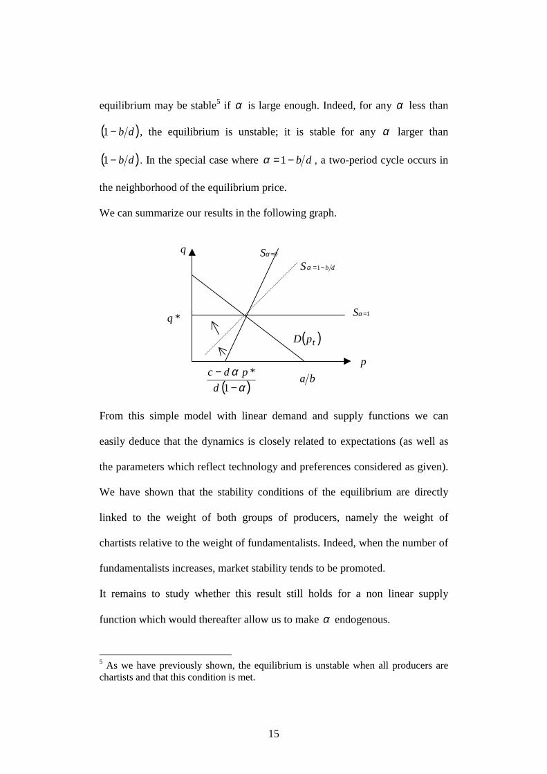
15

equilibrium may be stable5 if α is large enough. Indeed, for any α less than

( )db−1 , the equilibrium is unstable; it is stable for any α larger than

( )db−1 . In the special case where db−=1α , a two-period cycle occurs in

the neighborhood of the equilibrium price.

We can summarize our results in the following graph.

From this simple model with linear demand and supply functions we can

easily deduce that the dynamics is closely related to expectations (as well as

the parameters which reflect technology and preferences considered as given).

We have shown that the stability conditions of the equilibrium are directly

linked to the weight of both groups of producers, namely the weight of

chartists relative to the weight of fundamentalists. Indeed, when the number of

fundamentalists increases, market stability tends to be promoted.

It remains to study whether this result still holds for a non linear supply

function which would thereafter allow us to make α endogenous.

5 As we have previously shown, the equilibrium is unstable when all producers arechartists and that this condition is met.

p

q

*q 1=αS

0=αSdbS −=1α

ba( )αα−

−1

*d

pdc

( )tpD

16

5. Non linear Cobweb dynamics

Our framework is based on the basic cobweb model derived from Hommes

(1999). While the demand function is still linear the supply function is not.

The linear demand function is defined by ( ) tt pBApD −= where B,A are

both positive parameters. The supply curve is S-shaped and equals

( ) ( ) 11 1 +−= dtt p̂p̂S , where d is an odd integer. Such a supply curve can

be easily derived from an increasing and convex cost function given by at least

a third order polynomial.

When the expectations are not specified, the dynamics is given by:

( )[ ]d/tt p̂

BBAp 1111 −−−= (1)

When tt pp̂ = , there is perfect foresight and we can then compute the rational

expectations steady state denoted by *p . A convenient feature of the cobweb

model is the uniqueness of the RE equilibrium. In the sequel we simulate the

cobweb model for different specification of the expectations functions.

First let us assume that expectations are homogeneous. More specifically let us

say these expectations are naive or myopic, i.e. when 1−= tt pp̂ , (1) becomes:

( )[ ]d/tt p

BBAp 1

1 111 −−−= −

17

In this case, there is a single group of agents and therefore no switching

function. Depending on the values of the parameters ( )dBA ,, , the REE is

stable (see Figure 1 in the Appendix) or unstable.

Second let us assume that expectations are heterogeneous. In this case, two

groups of agents coexist: the chartists and the fundamentalists. Each group has

his own way to formulate expectations:6

- Chartists have myopic expectations: 1−= tt pp̂ ,

- Fundamentalists consider that the expected price is always equal to the

steady state price: *pp̂t = .

Following Hommes (1999) we assume that the weighting of both groups is

exogenous. We denote by [ ]10,∈α the weight associated with fundamentalists.

(1) becomes:

( )( )[ ]d/tt *pp

BBAp 1

1 1111 −+−−−= − αα (2)

We simulate (2) for a broad range values of parameters A, B and d and also for

different weighting, i.e. for various values of α .

In any case, the REE is unique. Depending on the values of the parameters

( )α,,, dBA , this REE can be either stable or unstable.

6 Many expectations functions are consistent with both behaviours, we consider thesimplest functions.

18

Consider first the case of a stable REE. If there are initially few

fundamentalists, it remains stable7 when the weight of fundamentalists

increases. However, when the REE is initially unstable8 for a low α , as soon

as the weight of fundamentalists increases, a two-period cycle emerges.

Thereafter the REE becomes stable for higher values of α .

The simulations results show that fundamentalists play a role in stabilizing the

economy. So, it remains to be shown if the same stabilizing effect is

associated with the increasing weight of fundamentalists for any endogenous

switching function.

Following Federici and Gandolfo (2000), we now assume that the switching is

endogenous and symmetric. (1) is becoming:

( )( )[ ]d/tttt *pp

BBAp 1

1 1111 −+−−−= − αα (3)

and the switching process, based on the deviation of the price from its

equilibrium value, is defining by:

( )21111

*pptt

−+−=

−βα .

As soon as the current price is far from the REE price, the weight of chartists

decreases. It is important to note that this process is symmetric, i.e. the

7 See Figure 2 in the Appendix where the dynamical path of prices is drawn for agiven value of α .8 The instability is provided by the values of the other parameters, namely ( )dBA ,, .

19

elasticity of the weighting w.r.t. the price deviation remains the same whatever

the sign of the deviation.

From the simulations results we deduce the following (given values of the

parameters9). If the REE is stable10 (respectively unstable) for a given initial

value of alpha, then it remains stable (respectively unstable) for any α . In

other words, the switching does not influence the stability conditions. More

specifically, the weight of fundamentalists does not imply the stabilizing effect

that appears in the exogenous switching case.

This apparently strange result may be explained by the features of the

switching function. Indeed, it appears that, when evaluated at the equilibrium

price *p , this function is equal to zero and therefore it may not have an

influence on the slope of the dynamics.

Given the previous result, it appears necessary to keep an endogenous

switching process but to remove its symmetry.

Recall that at any period, we must have [ ]10,t ∈α and the dynamics of prices

is still given by (3).

Our switching process, based on the fluctuations of past prices, is now

asymmetric. Its specification depends on a given evolution of past prices.

When past prices increased, few number of fundamentalists may turn to be

9 However, the results hold for any β .10 See Figure 3 in the Appendix.

20

chartist. When there is a downward trend in prices, a large number of chartists

may turn to be fundamentalist.

In our simulations, the following asymmetric specification of tα has been

chosen:

When the past prices increased ( 021 >− −− tt pp ), there are more chartists, i.e.

tα decreases, but we assume that tα decreases slowly.

When the past prices decreased ( 021 <− −− tt pp ), there are less chartists, i.e.

tα increases, but we assume that tα increases faster.

Consequently, the dynamics of the weighting is clearly asymmetric.

For ease of understanding, let us introduce the following notations:

21 −− −= tt ppx and 1−−= tty αα and draw a diagram of our specification.

x

y

y=-x

Each branch of the lines represents the switching process and is given by:

21

( )ε+−= 1xy

with γε −= if 0>x ,

and with γε 1= if 0<x ,

and in both cases [ ]10,∈γ .

The dynamics now includes two dynamical variables (the weighting and the

price). We deal with a two-dimensional dynamical system described by:

- the dynamics on prices (3)

- the dynamics on tα (i.e. the switching process).

The results from simulations are the following.11 For any values of the

parameters, the unique REE is stable. On the transition path, the values taken

by tα are increasing, i.e. the stability is associated with an increase of the

weight of fundamentalists.

6. Concluding comments

In a simple cobweb model we have shown that the introduction of

heterogeneous beliefs and of the possibility of switching of behaviour allow

the economy to shift from instability to stability. This shift is attributed to the

increase of the weight of fundamentalists in the case of an exogenous

switching. While we have focused our attention on how the weight of each

group influences the stability/instability result, it should be noted that it will

also have an impact on the speed of convergence to the REE.

11 See Figure 4 in the Appendix.

22

When we have considered an endogenous and symmetric switching process,

the economy may remain unstable.

However, when the endogenous switching process is asymmetric and based on

past prices, then stability is always obtained and is associated with an increase

of the number of fundamentalists. This latter result confirms the widespread

belief that fundamentalist market behaviour as compared with that of chartist

tends to promote market stability.

Acknowledgements

This paper was presented at the 2001 MMF (Money, Macro and Finance

Group) conference in Belfast, UK. We wish to thank the participants of the

MMF conference for their constructive comments. Errors remain ours.

References

Bask, M. (1998), Chartists and fundamentalists in the foreign exchange

market: forecasting horizons and exchange rate dynamics, Working Paper

465d, Department of Economics, Umea University.

De Grauwe, P., Dewachter, H. and Embrechts, M. (1993), Exchange rate

theory: chaotic models of exchange rate, Oxford, Blackwell.

Federici, D. and Gandolfo, G. (2000), Is there chaos in the Italian exchange

rate? mimeo.

23

Frankel, J.A. and Froot, K. A. (1990a), Chartists, fundamentalists and the

demand for dollars, in Private behaviour and government policy in

interdependent economies, edited by A. S. Courakis and M. P. Taylor,

Clarendon Press: Oxford.

Frankel, J.A. and Froot, K. A. (1990b), Chartists, fundamentalists, and trading

in the foreign exchange market, American Economic Review 80(2), 181-185.

Hommes, C. (1999), Cobweb dynamics under bounded rationality. CeNDEF

Working Paper 99-05, University of Amsterdam.

Kaizoji, T. (1999), Complex dynamics of speculative price, Complexity

International 6, 21 pages.

Lasselle, L., Svizzero, S., and Tisdell, C. (2001), Diversity, globalisation and

market stability, forthcoming in Economia Internazionale.

Lucas, R. E. (1971), Econometric testing of the natural rate hypothesis, in The

econometrics of price determination conference, Board of governors of the

federal reserve system and social science research council, edited by O.

Eckstein.

Muth, J. F. (1961), Rational expectations and the theory of price movements,

Econometrica 29, 315-335.

Vigfusson, R. (1996), Switching between chartists and fundamentalists: a

Markov switching approach, Bank of Canada, Working Paper 96-1.

Witt, C. A. and Witt, S. F. (1995), Forecasting tourism demand: a review of

empirical research, International Journal of Forecasting 11(3), 447-475.

24

Appendix

In the following simulations, the values of the parameters are:

A = 2.5, B = 0.2, and d = 5. Please note that the initial price is denoted by

1p where 1 is the initial period of time.

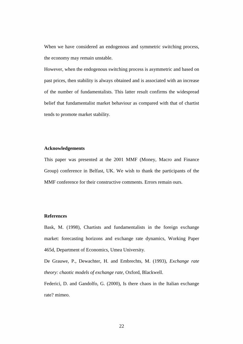
Figure 1: homogeneous expectations

531 .p =

2 4 6 8 10 12 14

1.5

2.5

3

3.5Prices Path

Value of the REE, p* = 2.26189.

Figure 2: heterogeneous expectations and exogenous switching process

Let 70.=α and 3618921 .p =

4 6 8 10

2.24

2.26

2.28

2.32

2.34

2.36

Prices Path

Value of the REE, p* = 2.26189.

25

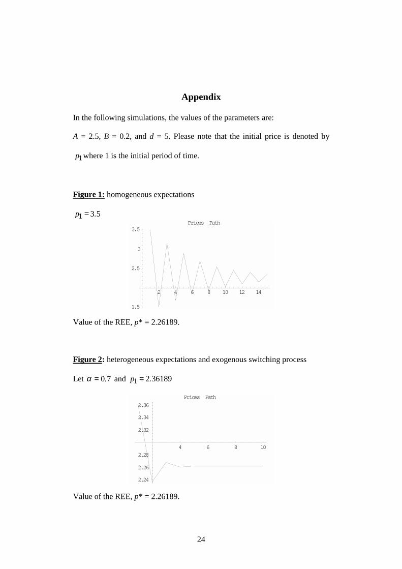
Figure 3: heterogeneous expectations and endogenous symmetric switching

process

Let 30.=β and 3618921 .p =

4 6 8 10

2.225

2.25

2.275

2.3

2.325

2.35

Prices Path

Value of the REE, p* = 2.26189

Figure 4: heterogeneous expectations and endogenous asymmetric switching

process

50.=γ , 221 .p = , 422 .p = , 102 .=α

p* = 2.26189

2 3 4 5 6 7

2.25

2.3

2.35

2.4Prices Path

Prices Path: {2.2, 2.4, 2.18398, 2.26526, 2.26163, 2.26191, 2.26189}

26

2 3 4 5 6

0.4

0.5

0.6

0.7

0.8

0.9

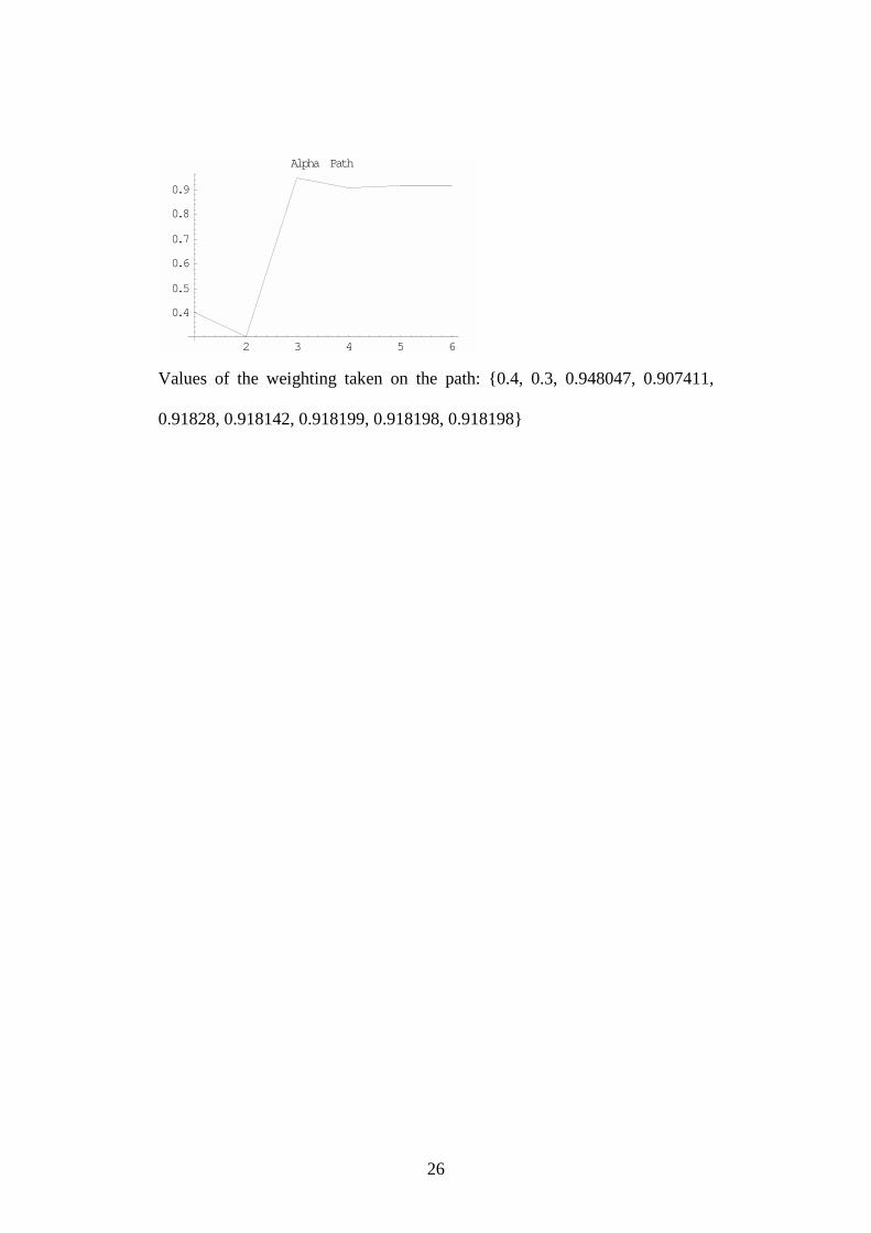
Alpha Path

Values of the weighting taken on the path: {0.4, 0.3, 0.948047, 0.907411,

0.91828, 0.918142, 0.918199, 0.918198, 0.918198}

27