Forward Premium Puzzle and Heterogeneous Beliefs

Abstract

We propose a two-country model with heterogeneous beliefs to understand the forward premium

puzzle. The domestic and foreign investors disagree on the expected growth rate of the domestic

money supply. Facing a shock to domestic money supply, the disagreement between the domestic

and foreign investors shifts the relative wealth of foreign investor, which moves the foreign exchange

rate and interest rate differential between foreign and domestic countries in opposite directions.

Calibrated to the U.S. and U.K. data, our model reproduces the rejection of the uncovered interest

rate parity. Using a monthly index of heterogeneous beliefs based on the Consensus Forecast in

15 major economies, the empirical evidence confirms two implications of our model: 1) a positive

relation between heterogeneous beliefs and changes in exchange rate; 2) a negative relation between

heterogeneous beliefs and carry trade returns.

JEL Classification: D53, G10, G12

Keywords: Heterogeneous beliefs; Uncovered interest rate parity; Carry trade; Exchange rate

volatility

1 Introduction

The failure of uncovered interest rate parity (UIP) has attracted academic attention for a few

decades. The UIP predicts that the expected change of the exchange rate (i.e., the price of domestic

currency in terms of foreign currency) should be equal to the nominal interest rate differential

between foreign and domestic countries. If the uncovered interest parity holds, a regression of the

realized exchange rate changes on the interest rate differentials should have a unity slope coefficient

and a zero constant. Contrary to the theoretical prediction, the empirical results find a negative

relation between the changes in exchange rate and the corresponding interest rate differential, with

the slope coefficient less than negative one (e.g., Hansen and Hodrick, 1980; Fama, 1984; Backus,

Foresi, and Telmer, 2001 ). This is called the “forward premium puzzle.” The empirical failure

of UIP implies that investors can employ currency carry trade strategy to earn a positive average

excess return by shorting the currency with low interest rate and investing the funds in the currency

with high interest rate.

To provide an explanation of the forward premium puzzle, we construct a heterogeneous belief

model building on Lucas (1982) and Croitoru and Lu (2015). In an economy with two groups of

investors from two countries, there are one consumption goods and one currency from each country.

The monetary policy of foreign country is transparent and thus both domestic and foreign investors

have the correct estimates about the growth rate of foreign money supply. However, the monetary

policy of domestic country is ambiguous or less transparent, in the sense that the expected growth

rate of domestic money supply is unobservable. Domestic and foreign investors may disagree on

the expected domestic money growth. In particular, domestic investors are more optimistic while

foreign investors are more pessimistic about domestic money growth. They “bet” against each

other on domestic monetary policy generating “trading risk” (e.g., David, 2008; Croitoru and Lu,

2015).

The key to produce the failure of UIP is to identify a friction making the changes in exchange

rate opposite to the interest rate differential. Our model reveals that the heterogeneity in beliefs

between domestic and foreign investors shifts the relative wealth weight of foreign investors, which

positively affects foreign exchange rate and negatively affects the interest rate differential. When

1

there is a negative shock to domestic money supply, domestic investors “lose” the bet because they

are overly optimistic about the domestic money growth rate and thus their relative wealth decreases.

They save less to smooth the consumption. The domestic nominal interest rate then rises, leading

to lower nominal interest rate differential between foreign and domestic countries. Meanwhile, ev-

erything else being equal, a negative shock to domestic money supply is likely to cause deflation,

making domestic goods relatively more competitive. Such an increase in foreign demand for do-

mestic goods leads to more demand for domestic currency and a currency appreciation. Moreover,

as the domestic money supply experiencing a negative shock, pessimistic foreign investors “win”

the bet because they are correct about the subsided domestic money growth rate and thus their

relative wealth increases. They consume more domestic consumption goods in addition to foreign

consumption goods through holding more domestic currency. Therefore, the domestic currency

further appreciates. Taken together, our model not only generates a negative relation between

the change in foreign exchange rate and the interest rate differential, but also produces a higher

volatility for the change in foreign exchange rate than the interest rate differential.

In addition to rationalize the well-documented empirical failure of UIP, our model can produce

a stochastic volatility of exchange rate with a magnitude comparable to the actual data. In our

model, “trading risk”, generated by the “bet” between domestic and foreign investors, amplifies

the diffusion coefficient of nominal exchange rate caused by domestic monetary risk, making the

volatility of nominal exchange rate rate positively related to investors’ heterogeneity in beliefs.

Consequently, the volatility of exchange rate fluctuates as the dispersion of beliefs varies over

time. This is consistent with the empirical findings in Beber, Breedon, and Buraschi (2010), which

documents a positive impact of differences in beliefs on the currency return volatility.

We calibrate our two-country model to the U.S. and U.K. data. Following the standard long-

horizon predictive regression approach like Fama (1984), we test the UIP directly by regressing the

changes in exchange rate on the interest differential. The slope coefficient in our baseline calibration

is negative (-1.01) and closely matches the actual data (-1.18). Our model could not only produce

the negative correlation between the currency risk premium and the interest rate differential, but

also generates higher volatility of foreign exchange rate (6.78%) than the volatility of interest

differentials (1.46 bps). The high volatility of the exchange rate in the model is associated with the

2

time-varying degree of heterogeneous beliefs. Using a proxy for the realized heterogeneous beliefs

in the U.S. and the U.K., the dynamics of the model generated exchange rate volatility resembles

the actual volatility dynamics of the USD/GBP exchange rate.

The calibration uncovers two testable implications of our model. First, the changes in the ex-

change rate are positively related to the heterogeneity in beliefs among investors about the domestic

money growth rate. Second, the carry trade return is negatively related to the heterogeneous be-

liefs. We test these two hypotheses in 15 major economies by constructing a monthly index of the

dispersion of beliefs using the Consensus Forecast published by the Consensus Economics. The

Consensus Forecasts contains the estimates of individual panelists for numerous macroeconomic

indicators. Our proxy of heterogeneous beliefs is based on the dispersion of the panelists’ estimate

for the consumer price index (CPI). To test the first hypothesis, the future changes in foreign ex-

change rates are regressed on the proxy of heterogeneity in beliefs and other control variables. The

evidence is overall supportive. The coefficients of dispersion of beliefs are positive in 10 out of the

15 economies, and 8 of them are statistically significant. For the second hypothesis, we regress the

3-month carry trade returns on the dispersion of beliefs. Out of the 15 countries, the regression

coefficients for 12 economies have the negative sign, and 9 of them are statistically significant. Our

results are robust to controlling for economic uncertainty, as well as using the relative proxy of

heterogeneity in beliefs. The relative heterogeneity in beliefs measures the dispersion of beliefs in

each country relative to the United States.

Our model is related to several studies that attempt to explain the forward premium puzzle.

Verdelhan (2010) provides a habit formation model to produce the failure of UIP. Heyerdahl-Larsen

(2014) extends Verdelhan (2010) to a model with consumption home bias and deep habits. In

addition to solving for the forward premium puzzle, it can match the dynamics of domestic assets

including equity premium, stock return volatility, and upward-sloping real yield curves. Burnside,

Han, Hirshleifer and Wang (2011) provide an explanation for the forward premium puzzle assuming

investors are overconfident about inflation information. Yu (2013) presents a sentiment-based model

which helps explain the forward premium puzzle and the low correlation between consumption

growth growth differentials and exchange rate growth. With the same purpose, Osambela (2013)

develops a two-country two-good model where domestic and foreign investors have different beliefs

3

about the expected output growth rate in each country. Our paper is most closely related to

Osambela (2013). However, there are two differences. First, in our model domestic and foreign

investors have different beliefs about the expected domestic money growth, and then we examine

the nominal forward premium puzzle. Second, our model generates high exchange rate volatility

due to “trading risk”, which is comparable to actual data.

Our model is also related to international asset pricing models with heterogeneous beliefs. Li

and Muzere (2010) present a model with two countries and two goods in which investors with

logarithmic utility have heterogeneous beliefs about expected output growth rate. They find that

the exchange rate and stock returns exhibit high volatility. Unlike their paper, we also explain

the nominal forward premium puzzle. Dumas, Lewis, and Osambela (2017) propose a sentiment

model in which domestic and foreign investors have different beliefs about the information content

in public signals. They study several interesting issues such as the co-movement of returns and

capital flows, the home equity preference, the dependence of firm returns on home and foreign

factors, and the abnormal returns around the listings of foreign firms in the home market. Unlike

their paper, our model extends Croitoru and Lu (2015) to an international setup where domestic

and foreign investors have heterogeneous beliefs about domestic monetary policy. The research

questions addressed are also different from Dumas, Lewis, and Osambela (2017). Moreover, our

model is related to two-tree models with heterogeneous beliefs. Buraschi, Trojani, and Vedolin

(2014) explain the differential pricing of index and individual equity options. Gallmeyer, Jhang,

and Kim (2016) demonstrate that the idiosyncratic cash flow shocks priced via the heterogeneity

in beliefs can explain cross-sectional stock returns and cash flows. Han, Lu, and Zhou (2018) show

that disagreement among investors in one large firm (i.e., industry leading firm) has a spillover

effect on the pricing of other stocks owned by these investors.

The rest of the paper is organized as follows. Section 2 describes the model and solves the

dynamic equilibrium. Section 3 calibrates parameters, reproduces several stylized empirical facts,

and derives two testable hypotheses. Empirical analysis results are presented in Section 4. Section

5 concludes the paper. The Appendix contains the proof of Propositions.

4

2 The Model

Our model builds on Lucas (1982) two-country model and Croitoru and Lu (2015) heterogeneous

beliefs model. We consider a continuous-time, pure exchange, finite horizon [0,T], and nominal

economy with two groups of investors from two countries. We call them domestic country and

foreign country respectively, and then domestic investors and foreign investors correspondingly.

The uncertainty is generated by a four-dimensional Brownian motion, ω = (ωε, ωε∗ , ωM , ω∗M )T .

There are one consumption goods and one currency from each country. The domestic consumption

goods is assumed to be the numeraire.

2.1 Aggregate Consumption, Money Supply, and the Information Structure

The aggregate consumption goods of domestic country and foreign country are denoted by ε and

ε∗, respectively. The money supplies in currency of domestic country and foreign country are

represented by M and M∗, respectively. They follow the dynamics given by:

d ln εt

d ln ε∗t

d lnMt

d lnM∗t

=

µε

µε∗

µM

µM∗

dt+

σεε 0 0 σεM∗

σε∗ε σε∗ε∗ 0 σε∗M∗

σMε σMε∗ σMM 0

0 σM∗ε∗ 0 σM∗M∗

dωt, (1)

where dω = (dωε, dω∗ε , dωM , dω

∗M )T and the four Brownian motions ωε, ω

∗ε , ωM , and ω∗M are inde-

pendent. We can allow these four Brownian motions to be dependent but this does not generate

new insights.

All investors can observe the processes of domestic and foreign aggregate consumption, ε and

ε∗, and money supplies, M and M∗. There is no uncertainty associated with domestic and foreign

consumption risks in the sense that all investors can observe the realizations of ωε and ω∗ε . Moreover,

the monetary policy of foreign country is transparent and thus all investors have the correct estimate

about the growth rate of foreign money supply, µ∗M . However, the monetary policy of domestic

country is ambiguous, in the sense that the expected growth rate of its money supply, µM , is

unobservable. All investors need to estimate it by observing the realizations of domestic money

5

supply, M . Thus, domestic and foreign investors may have different estimates about µM . We

denote their estimates by µDM and µFM , respectively.1 The dynamics of domestic money supply

from the perspective of each investor (i = D,F ) follows the dynamics given by:

d lnMt = µiMdt+ σMεdωε,t + σMε∗dωε∗,t + σMMdωiM,t, (2)

where investor i’s perceived innovation process of domestic monetary risk dωiM,t = 1σMM

(dMtMt−

µiMdt− σMεdωε,t − σMε∗dωε∗,t) and then we have:

dωFM,t = dωDM,t + µMdt, (3)

where µM =µDM−µ

FM

σMMdenotes the difference in estimated growth rate of domestic money supply

between domestic and foreign investors, scaled by the standard deviation of domestic money supply.

2.2 Investment Opportunities

There are four uncertainties, so we need five securities to complete the market: one real riskless

bond, B, with zero-supply and paying-off the real interest rate r; two zero-supply, nominally riskless

bonds, BM and B∗M , in its own currency paying-off nominal interest rate R and R∗ (but they are

risky in real items); and two stocks S and S∗ representing the claims on domestic and foreign

aggregate consumption ε and ε∗ respectively, and with a supply of one share. The prices of the

riskless bond, two nominally riskless bonds, and two stocks follow the dynamics:

dBt = Btrtdt, (4)

dBM,t = BM,t[(µq,t +Rt)dt+ σq,tdωt] = BM,t[(µiq,t +Rt)dt+ σq,tdω

it],

dBM∗,t = BM∗,t[(µq∗,t +R∗t )dt+ σq∗,tdωt] = BM∗,t[(µiq∗,t +R∗t )dt+ σq∗,tdω

it],

dSt + εtdt = St(µS,tdt+ σS,tdωt) = St(µiS,tdt+ σS,tdω

it),

dS∗t + p∗t ε∗tdt = S∗t (µS∗,tdt+ σS∗,tdωt) = S∗t (µiS∗,tdt+ σS∗,tdω

it),

where p∗ is the equilibrium price of foreign consumption goods relative to the price of domestic

consumption goods (which is the numeraire), dωi = (dωε, dω∗ε , dω

iM , dω

∗M )T is innovation process

1We can assume investors update their estimates about the expected domestic money growth rate using Bayesianlearning, but this doesn’t generate any new insight.

6

perceived by investor i, and the volatility matrix is given by

Ω =

(σq, σ∗q , σS , σ∗S

)T=

σqε σqε∗ σqM σqM∗

σq∗ε σq∗ε∗ σq∗M σq∗M∗

σSε σSε∗ σSM σSM∗

σS∗ε σS∗ε∗ σS∗M σS∗M∗

. (5)

Therefore, we have the following relationship(µDq − µFq , µDq∗ − µFq∗ , µDS − µFS , µDS∗ − µFS∗

)=

(σqM, σq∗M , σSM, σS∗M

)µM . (6)

Given a complete market, investor i faces the unique market prices of risk, θε, θε∗ , θiM and θ∗M .

They are associated with the uncertainties of domestic and foreign consumption goods and money

supplies, respectively, and solve for the following equation (i = D,F ):

Ω

(θε, θε∗ , θiM , θ∗M

)T=

(µiq − r, µiq∗ − r, µiS − r, µiS∗ − r

)T. (7)

Therefore,

θDM − θFM = µM . (8)

Under the no arbitrage condition and assuming domestic consumption goods as the numeraire,

investor i’s perceived state price density in equilibrium is given by (e.g., Buraschi, Trojani, and

Vedolin, 2014)

dξit = −ξit(rtdt+ θε,tdωε,t + θε∗,tdωε∗,t + θiM,tdωiM,t + θM∗,tdωM∗,t), (9)

where rt is the domestic real interest rate.

2.3 Investors’ Optimization

We assume that all investors consume both domestic and foreign consumption goods. Foreign in-

vestors are assumed to hold both foreign and domestic currencies, while domestic investors only hold

domestic currency. Investor i (i = D,F ) chooses his holdings of domestic and foreign consumption

7

and currencies and maximizes his cumulative lifetime expected utility

maxci,c∗i,mi,m∗i

Eit

[∫ T

0e−ρtui

(cit, c

∗it , qtm

it,q∗tm

∗it

p∗t

)dt

](10)

s.t. Eit

[∫ T0 ξ

it

(cit + p∗t c

∗it + qtm

it + q∗tm

∗it

)dt]≤ xi0,

where

uD(cD, c∗D, qmD, q

∗m∗D

p∗

)= α

[βD log

(cD)

+(1− βD

)log(c∗D)]

+ (1− α) log(qmD

),

uF(cF , c∗F , qmF , q

∗m∗F

p∗

)= α

[(1− βF

)log(cF)

+ βF log(c∗F)]

+ (1− α)[(1− γ) log

(qmF

)+ γ log

(q∗m∗F

p∗

)],

where q and q∗ denote the equilibrium prices of domestic currency and foreign currency relative to

the price of domestic consumption (numeraire).

Following Basak and Cuoco (1998) and Basak (2000), we can construct a “world” representative

agent with the following utility function:

U(ct, c∗t , qtmt,

q∗tm∗t

p∗t;λt) (11)

= maxcD+cF=c,c∗D+c∗F=c∗

mD+mF=m,m∗D+m∗F=m∗

uD(cDt , c

∗Dt , qtm

Dt ,

q∗tm∗Dt

p∗t

)+ λtu

F(cFt , c

∗Ft , qtm

Ft ,

q∗tm∗Ft

p∗t

),

where λ denotes the relative wealth weight of foreign investors, and it is positive and can be

stochastic.

2.4 The Equilibrium

We derive the competitive equilibrium following the standard martingale techniques (e.g., Cox and

Huang, 1989; Karatzas, Lehoczky, and Shreve, 1990).

Definition 1 An equilibrium is a price system (r,R,R∗, S, S∗, BM , BM∗) and admissible policies(ci, c∗i,mi,m∗i, πi

)(i = D,F ) such that: (i) investors choose their optimal policies given their

beliefs; and (ii) markets for consumption, money and securities clear, i.e.,

cDt + cFt = εt, c∗Dt + c∗Ft = ε∗t , (12)

mDt +mF

t = Mt, m∗Dt +m∗Ft = M∗t ,

πDM,t + πFM,t = 0, πDM∗,t + πFM∗,t = 0,

πDS,t + πFS,t = 1, πDS∗,t + πFS∗,t = 1,

XDt +XF

t = St + p∗tS∗t + qtMt + q∗tM

∗t .

8

In the following proposition, we present the domestic and foreign nominal interest rates and the

market prices of domestic and foreign consumption risk and monetary risk.

Proposition 1 The domestic and foreign nominal interest rates are

Rt = 1+(1−γ)λtGDt +(1−γ)GFt λt

, (13)

R∗t = 1Ht, (14)

where λ is the relative wealth weight of foreign investors and follows the dynamics

dλt = −λtµMdωDM,t, (15)

and Git =exp(

12σ

2M−µ

iM

)(T−t)

−1

12σ

2M−µ

iM

(i = D,F ), and Ht =exp(

12σ

2M∗−µM∗

)(T−t)

−1

12σ

2M∗−µM∗

.

The market prices of of domestic and foreign consumption and monetary risk perceived by twocountries’ investors are

θε,t = σεε, θε∗,t = 0, (16)

θM∗,t = σεM∗ ,

θDM,t =(1−βF )λtµMβD+(1−βF )λt

, θFM,t = − βDµMβD+(1−βF )λt

.

Equation (13) shows that investors’ disagreement about the expected domestic money growth

rate, µM , affects the domestic nominal interest rate in two ways. First, the investors’ disagreement

shifts the relative wealth weight of foreign investors, λ. Second, the disagreement affects µiM and

then Git. In the presence of the investors’ disagreement, a negative shock to domestic money supply

moves the domestic nominal interest rate higher. Facing a negative shock to domestic money

supply, optimistic domestic investors “lose” the bet because they overestimate the growth rate

of domestic money supply and thus their relative wealth decreases (Equation (15)). Therefore,

domestic investors save less, pushing domestic nominal interest rate up.

Equation (14) shows that foreign nominal interest rate is nonstochastic. This is intuitive: first,

there is no uncertainty associated with foreign money supply; second, the foreign currency is only

held by foreign investors. Admittedly, we could instead assume that both domestic and foreign

investors hold the foreign currency. Then, the foreign nominal interest rate, which depends on

investors’ disagreement and relative wealth, would become stochastic. This might help our model

match the actual data better including the first and second moment of the foreign nominal interest

rate. However, this alternative assumption is not able to generate any new insight in explaining

9

the nominal forward premium puzzle.

Equation (16) describes the individual market prices of domestic and foreign consumption risk

and monetary risk, respectively. The expected growth rate of domestic money supply is unob-

servable and thus domestic and foreign investors may have different perceptions about domestic

monetary shock. Therefore, they have different perceived market price of domestic monetary risk.

Foreign investors are relatively pessimistic and transfer domestic monetary risk to domestic in-

vestors in order to smooth their consumption. Domestic investors require a higher premium for

risk compensation and hence a higher perceived market price of monetary risk. The individual

market price of domestic monetary risk is affected by investors’ disagreement through two chan-

nels. First, disagreement directly affects individual market price of domestic monetary risk through

risk-sharing effect. Second, the disagreement shifts wealth allocation between domestic and foreign

investors, λ, and then affects individual market price of domestic monetary risk. This is consistent

with the analysis of Croitoru and Lu (2015).

In the following, we present the forward interest rates for zero-coupon domestic and foreign

bonds.

Remark 1 The time t forward interest rate for (n −m)-year zero-coupon domestic bond startingin m years (n > m > 0) is given by

ft,m,n =(1+Rt,n)n

(1+Rt,m)m − 1, (17)

where the time t zero-coupon yield with maturity τ(τ = m,n) for domestic bond is

Rt,τ = 1τ ln(

GDt +(1−γ)GFt λt]

GDt+τ exp

(12σ

2M−µ

DM )τ

+(1−γ)GFt+τ exp

(12σ

2M−µ

FM )τ

λt

). (18)

The time t forward interest rate for (n − m)-year zero-coupon foreign bond starting in m years(n > m > 0) is given by

f∗t,m,n =(1+R∗t,n)n

(1+R∗t,m)m − 1, (19)

where the time t zero-coupon yield with maturity τ(τ = m,n) for foreign bond is

R∗t,τ = µFM − 12σ

2M − 1

τ ln(Ht+τHt). (20)

Similar to the analysis for domestic nominal interest rate, Equation (17) shows that the forward

interest rate for domestic bond is affected by the disagreement about domestic monetary policy.

However, due to its complicated expression, it is difficult to analyze the relation forward interest

10

rate and disagreement. We leave this issue in the section of numerical analysis. Moreover, it is not

surprising that the foreign foreign interest rate is unaffected by the disagreement with the same

intuition as that for foreign nominal interest rate.

The next proposition presents the nominal exchange rate and its dynamics.

Proposition 2 The nominal foreign exchange rate is

ent =GDt +(1−γ)λtGFt

γHtλt

M∗tMt. (21)

The drift of nominal foreign exchange rate perceived by domestic investors and its diffusion coeffi-cients are

µDen,t = µM∗ − 12σ

2M∗ − µDM + 1

2σ2M − σMε∗σM∗ε∗ (22)

−exp(

12σ

2M−µ

DM

)(T−t)

+(1−γ)λt exp

(12σ

2M−µ

FM

)(T−t)

GDt +(1−γ)λtGFt

+exp(

12σ

2M∗−µM∗

)(T−t)

Ht

+GDt (µM−σMM )µMGDt +(1−γ)λtGFt

,

σenε,t = −σMε, σenε∗,t = σM∗ε∗ − σMε∗ ,

σenM,t = −σMM +GDt µM

GDt +(1−γ)λtGFt, σenM∗,t = σM∗M∗ .

The nominal foreign exchange rate is the ratio of the relative price of domestic currency, q, to

the relative price of foreign currency, q∗. Equation (21) shows that nominal foreign exchange rate is

positively related to foreign money supply and negatively proportional to domestic money supply.

Moreover, nominal foreign exchange rate is driven by investors’ disagreement about the expected

domestic money growth rate. The intuition is similar to the effect of disagreement on individual

market price of domestic monetary risk. When there is a negative shock to domestic money supply,

the decrease in domestic money supply causes deflation in the domestic country, making domestic

goods relatively more competitive. This boosts the foreign demand for domestic goods, leading

to domestic currency appreciation. Consequently, the nominal exchange rate (denoted by units

of foreign currency per domestic currency) rises. More importantly, pessimistic foreign investors

“win” the bet because they have more accurate estimate about the subdued expected growth rate

of domestic money supply and thus their relative wealth increases. They consume more domestic

consumption goods through holding more domestic currencies. Hence, domestic currency further

appreciates, leading to additional increases in the nominal exchange rate.

Equation (22) shows that the drift and diffusion coefficients of nominal exchange rate are related

11

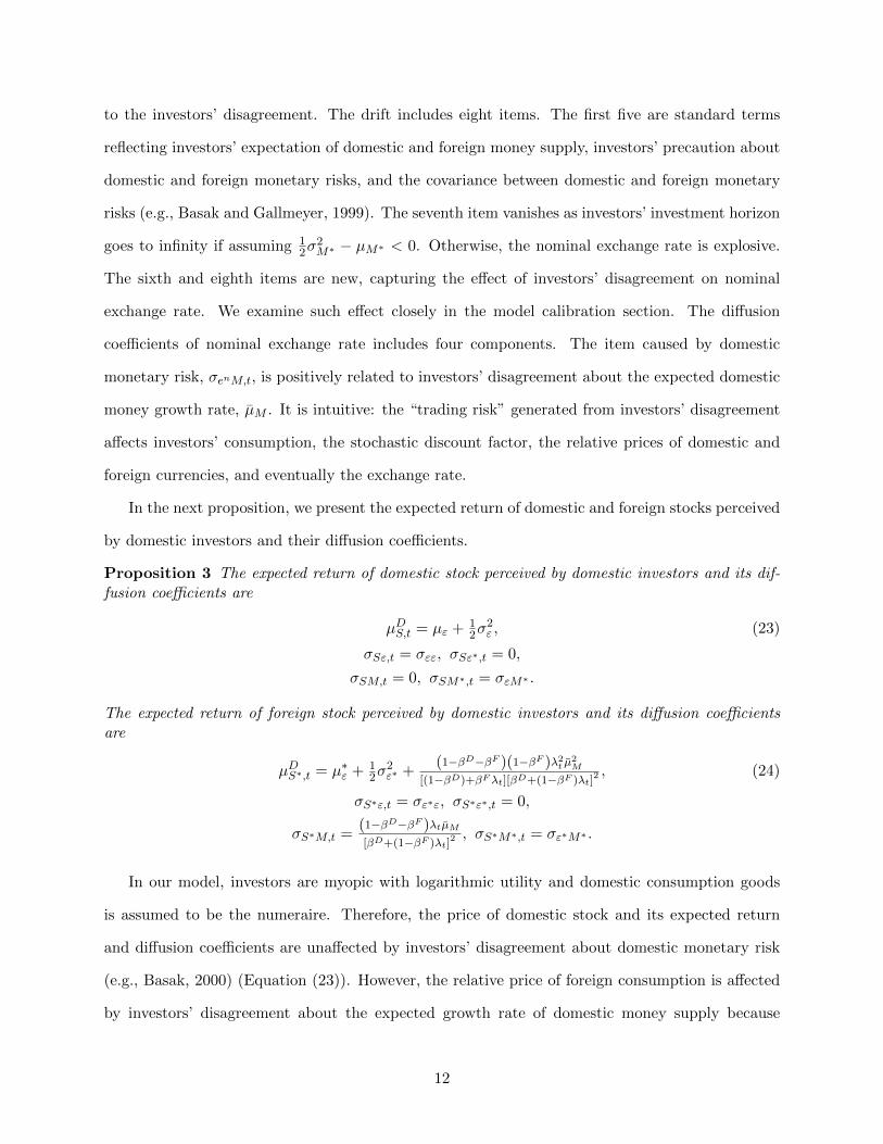
to the investors’ disagreement. The drift includes eight items. The first five are standard terms

reflecting investors’ expectation of domestic and foreign money supply, investors’ precaution about

domestic and foreign monetary risks, and the covariance between domestic and foreign monetary

risks (e.g., Basak and Gallmeyer, 1999). The seventh item vanishes as investors’ investment horizon

goes to infinity if assuming 12σ

2M∗ − µM∗ < 0. Otherwise, the nominal exchange rate is explosive.

The sixth and eighth items are new, capturing the effect of investors’ disagreement on nominal

exchange rate. We examine such effect closely in the model calibration section. The diffusion

coefficients of nominal exchange rate includes four components. The item caused by domestic

monetary risk, σenM,t, is positively related to investors’ disagreement about the expected domestic

money growth rate, µM . It is intuitive: the “trading risk” generated from investors’ disagreement

affects investors’ consumption, the stochastic discount factor, the relative prices of domestic and

foreign currencies, and eventually the exchange rate.

In the next proposition, we present the expected return of domestic and foreign stocks perceived

by domestic investors and their diffusion coefficients.

Proposition 3 The expected return of domestic stock perceived by domestic investors and its dif-fusion coefficients are

µDS,t = µε + 12σ

2ε , (23)

σSε,t = σεε, σSε∗,t = 0,

σSM,t = 0, σSM∗,t = σεM∗ .

The expected return of foreign stock perceived by domestic investors and its diffusion coefficientsare

µDS∗,t = µ∗ε + 12σ

2ε∗ +

(1−βD−βF )(1−βF )λ2t µ2M[(1−βD)+βFλt][βD+(1−βF )λt]

2 , (24)

σS∗ε,t = σε∗ε, σS∗ε∗,t = 0,

σS∗M,t =(1−βD−βF )λtµM[βD+(1−βF )λt]

2 , σS∗M∗,t = σε∗M∗ .

In our model, investors are myopic with logarithmic utility and domestic consumption goods

is assumed to be the numeraire. Therefore, the price of domestic stock and its expected return

and diffusion coefficients are unaffected by investors’ disagreement about domestic monetary risk

(e.g., Basak, 2000) (Equation (23)). However, the relative price of foreign consumption is affected

by investors’ disagreement about the expected growth rate of domestic money supply because

12

pessimistic (foreign) investors transfer monetary risk to optimistic (domestic) investors. Therefore,

the price of foreign stock and its expected return and diffusion coefficients are affected by investors’

disagreement, µM (Equation (24)). This is new in the literature: the disagreement about nominal

variable of domestic country (i.e., monetary policy) affects the price and its dynamics of real variable

(i.e., stock) of foreign country. Equation (24) also shows that the diffusion coefficient of expected

return of foreign stock caused by domestic monetary risk, σS∗M , is positively related to investors’

disagreement, µM and then the total volatility of stock return increases with the disagreement.

3 Numerical Analysis and Results

To test the validity of our model, we investigate if our model could replicate some well-documented

empirical findings in the literature. The first subsection calibrates the model to U.S. and U.K data.

We examine how heterogeneous beliefs are related to the volatility of the exchange rate. The next

subsection investigates the ability of the model to reproduce the rejection of uncovered interest rate

parity, as well as the joint relations between heterogeneous beliefs, changes in exchange rate, and

interest rate differentials.

3.1 Calibration

We calibrate the model parameters to match a set of unconditional moments on real consumption

growth, the money supply, the nominal interest rates, and the nominal foreign exchange rate.

Following Osambela (2013) and Heyerdahl-Larsen (2014), we consider the United States as the

domestic country and the United Kingdom as the foreign country. Our sample contains quarterly

observations from 1955 until 2016 obtained from Federal Reserve Economic Data (FRED) database.

The calibrated parameters of aggregate consumption and money supplies are directly matched

to unconditional mean and variance of real consumption growth and money supply growth in the

United States and the United Kingdom. Time discount factor ρ is set to 0.1, consistent with

previous studies (e.g., Dumas, Kurshev, and Uppal, 2009; Dumas, Lewis and Osambela, 2017).

Given the life expectancy in the United States and the United Kingdom sits at about 78, the

investment horizon is set at 60 years. The initial relative wealth weight of foreign investors, λ,

is normalized to 1. To calibrate other parameters in our model, we use the method of simulated

13

moments. Mathematically, let Λd be the moments of the data (e.g. mean or variance of real

consumption growth and the money supply). Denote Λs as the same moments calculated on the

simulated data from the model with parameters θ. The Λs is averaged across simulations. Then,

we obtain the calibrated parameters:

θMSM = arg min m(x, θ)′Wm(x, θ), (25)

where m(x, θ) = Λd − Λs and W is a positive-definite weighting matrix. We choose the weighting

matrix as a diagonal matrix with an inverse of empirical variances of the moments. Our moment

conditions target the mean and variance of real consumption growth and money supply, as well as

the mean of foreign exchange rate, domestic and foreign nominal interest rate. Table 1 presents

the chosen parameters.

[INSERT TABLE 1 HERE]

Using the calibrated parameters in Table 1, we simulate the model across 10,000 paths of 160

quarterly observations. Table 2 reports the unconditional moments of the data, as well as the

average moments obtained from our simulation. The first half of Table 2 reports the moments that

we target to match with the actual data. The second half corresponds to other moments that we

employ to evaluate the ability of our model to replicate some stylized facts concerning the currency

market. Overall, our model could produce comparable moments as the actual data. For example,

the second moments of the model-generated interest rate and interest rate differential match the

actual data closely. The model implied volatility of nominal interest rate is 0.84 bps and 0.96 bps

in the U.S. and the U.K. respectively. The corresponding moments of the actual data are 0.79 bps

and 0.92 bps. The volatility of interest rate differential is 1.46 bps in the model, compared to 1.07

bps in the data. The volatility of the foreign exchange rate in the model is 6.78%, which is slightly

higher than the 3.98% observed in the data. Noticeably, our model could also produce a higher

volatility of foreign exchange rate (6.78%) than the volatility of interest differentials (1.46 bps).2

Our model could also produce the correlation of money supply, interest rate, and consumption

growth similar to the actual data. The correlation between domestic and foreign interest rate is

2Heyerdahl-Larsen (2014) pointed out that “To reproduce the failure of the UIP, the currency risk premiummust...exhibit a higher volatility than the expected depreciation of the exchange rate.”

14

quite high both in the data (0.87) and our model (0.98). The correlation between domestic and

foreign consumption is about 0.24 in our model and the data. Our model produces a slightly lower

correlation between domestic and foreign money supply (0.12), compared to the actual data (0.26).

However, our model has difficulties in characterizing the moments of stock returns. The model

generates very low levels of the mean and standard deviation of the stock returns. Understandably,

the main purpose of our parsimonious model is to identify the effect of investors’ disagreement on

the dynamics of the exchange rate and interest rates. Consequently, the assumption of the stock

markets in the model might be overly simplified.

[INSERT TABLE 2 HERE]

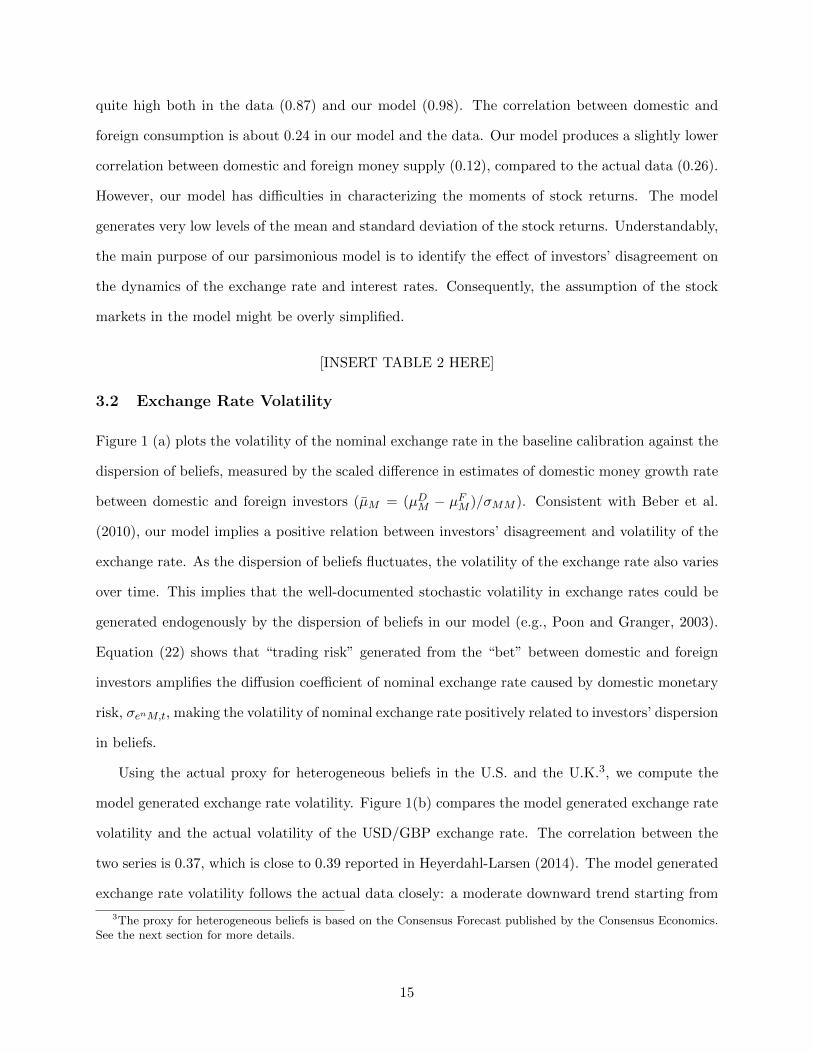
3.2 Exchange Rate Volatility

Figure 1 (a) plots the volatility of the nominal exchange rate in the baseline calibration against the

dispersion of beliefs, measured by the scaled difference in estimates of domestic money growth rate

between domestic and foreign investors (µM = (µDM − µFM )/σMM ). Consistent with Beber et al.

(2010), our model implies a positive relation between investors’ disagreement and volatility of the

exchange rate. As the dispersion of beliefs fluctuates, the volatility of the exchange rate also varies

over time. This implies that the well-documented stochastic volatility in exchange rates could be

generated endogenously by the dispersion of beliefs in our model (e.g., Poon and Granger, 2003).

Equation (22) shows that “trading risk” generated from the “bet” between domestic and foreign

investors amplifies the diffusion coefficient of nominal exchange rate caused by domestic monetary

risk, σenM,t, making the volatility of nominal exchange rate positively related to investors’ dispersion

in beliefs.

Using the actual proxy for heterogeneous beliefs in the U.S. and the U.K.3, we compute the

model generated exchange rate volatility. Figure 1(b) compares the model generated exchange rate

volatility and the actual volatility of the USD/GBP exchange rate. The correlation between the

two series is 0.37, which is close to 0.39 reported in Heyerdahl-Larsen (2014). The model generated

exchange rate volatility follows the actual data closely: a moderate downward trend starting from

3The proxy for heterogeneous beliefs is based on the Consensus Forecast published by the Consensus Economics.See the next section for more details.

15

the early 1990s and a high volatility period in the late 2000s. Noticeably, our model captures the

spike in volatility during the 2007-2009 financial crisis, albeit overshooting actual data.

[INSERT FIGURE 1 HERE]

3.3 The Uncovered Interest Rate Parity

Following Osambela (2013), this section verifies if our model could replicate the rejection of un-

covered interest rate parity (UIP). We run the UIP regression on three samples of data. First,

using the calibrated parameters as in Table 1, we simulate 10,000 paths of nominal interest rates

of the domestic and foreign markets as well as the nominal foreign exchange rate. We denote this

sample as the “baseline calibration.” Next, we simulate another 10,000 paths of nominal interest

rates and exchange rates without heterogeneous beliefs between the domestic and foreign investors.

In other words, we manually set the model parameters µFM = µDM = 2.15% while keeping other

parameters unchanged. We refer to this as the “no disagreement” sample. Lastly, we collect the

actual quarterly nominal interest rate and exchange rate in the U.S. and the U.K. between 1955

and 2016. For each of the three samples, we run time-series UIP regressions for each path i to

derive the estimated slope βi as well as the estimated intercept αi. Specifically, the UIP regression

is given as

et+1 − et = α+ β(RFt −RDt ) + εt, (26)

where the et is the natural log of exchange rate at time t, RDt and RFt are the domestic and foreign

interest rate at time t, respectively.4 If the UIP holds, then α = 0, β = 1. In other words, currencies

with high interest rate should depreciate, while the low interest rate currencies would appreciate.

Panel A of Table 3 reports the mean of slopes (β), the intercepts (α), the absolute value of t-

statistics (in parentheses), and the adjusted R-squared (R2). The baseline calibration suggests that

our model can reproduce the rejection of UIP as observed in the empirical data. The coefficient β in

our calibrated model (-1.01) is negative and closely resembles the one in the real data (-1.18). The

calibrated model reveals that, in contrast to the UIP, the currency with high interest rate appreciates

while the low interest rate currency depreciates. On the contrary, the “no disagreement” sample

4Note that the exchange rate et is defined as the price of the domestic currency divided by the price of foreigncurrency. An increase in et indicates a depreciation of the foreign currency or an appreciation of the domestic currency.

16

estimation exhibits a positive β. Without heterogeneous beliefs, our baseline model behaves more

similarly to what the standard UIP predicts. The calibration also shows that our model could

produce very low levels of R2, which is another notable feature of the empirical failure of UIP.

(Burnside, 2018)

[INSERT TABLE 3 HERE]

Recent empirical studies find that the forecasting horizon is important in determining the ex-

change rate predictability (Boudoukh, Richardson, and Whitelaw, 2016; Engle, 2016). In particular,

Engel (2016) shows that the estimated coefficient β in the UIP regression is negative for a short

forecasting horizon but becomes positive as the forecasting horizon increases. In other words, when

the interest rate increases, the currency appreciates in the short run, but depreciates in the longer

run. To reproduce the role of forecasting horizon in the UIP regression, we run the following

regression:

et+j+1 − et = α+ β(RFt −RDt ) + εt, (27)

where j is the forecasting horizon. If j = 0, then it becomes the traditional UIP regression in

(26). Panel B of Table 3 reports the model estimation for different horizons (j) and dispersion of

beliefs. The baseline calibration shows the coefficient β starts from -0.89 and increases above 0.03

as the forecasting horizon grows. In other words, the pattern of exchange rate predictability in our

model could change as the forecasting horizon extends.5 To further pin down the joint effect of

the heterogeneous beliefs and the forecasting horizon, we manually change the level of dispersion

of beliefs and test its impact on the UIP coefficient. In addition to the “no disagreement’ sample,

we simulate a “low disagreement” and a “high disagreement” sample. The “Low disagreement”

(“High disagreement”) sample comes from 10,000 simulations by setting the µDM − µFM = 0.12%

(µDM −µFM = 0.4%) while keeping other parameters unchanged. Without heterogeneous beliefs, the

β fluctuates around 0.38 and exhibits no upward trend as forecasting horizon increases. In the “low

5Although the UIP regression coefficient β flipped sign in the baseline calibration as in Engel (2016), we acknowl-edge that the increase in β is slower than what the actual data shows as the forecasting horizon j extends. In thebaseline calibration, the sign becomes positive only after 24 quarters. Engel (2016) shows that the sign flipping couldoccur within two years.

17

disagreement” sample, however, the β grows from -0.58 to 0.14. Meanwhile, the β rises even faster

for the “high disagreement” sample, from -5.44 to -1.59 as j grows. In summary, Panel B of Table

3 implies the heterogeneous beliefs could facilitate the changes in exchange rate predictability as

the forecasting horizon grows.

3.4 Carry Trade Returns, Changes in Exchange Rate and Heterogeneous Beliefs

The rejection of UIP implies that there is a high average payoff to the carry trade. The carry trade

is defined as a domestic investor who borrows at the domestic risk-free rate (RD), exchanges the

proceeds into foreign currency, invest it at the foreign risk-free rate (RF ), and eventually converts

all investment back into home currency. The carry trade returns from investing in the currency

market are given as:

CTRt+1 = RF −RD − (et+1 − et). (28)

With heterogeneous investors in our models, the dispersion of beliefs enters the pricing kernel

and thus naturally affects the expected currency returns. To illustrate the model implied relation

between heterogeneous beliefs and carry trade returns, we conduct a set of simulations using model

parameters as those in Table 1, while manually adjust the magnitude of heterogeneous beliefs. For

each value of µM , we simulate 10,000 paths and compute the average carry trade return. Figure

2 plots the model implied relation between heterogeneous beliefs (µM ) and average carry trade

return. Consistent with previous studies such as Beber et al. (2010) and Yu (2013), the carry trade

returns are negatively associated with the heterogeneity in beliefs.

[INSERT FIGURE 2 HERE]

Beber et al. (2010) decompose carry returns into “returns generated by the interest rate differ-

entials and the returns generated by exchange-rate appreciation/depreciation.” They find that the

carry trade return is negatively related to the dispersion of beliefs, while one of its component, the

interest rate differential, is positively related to the dispersion of beliefs. Therefore, it is particularly

essential to check the underlying model implied relations between the heterogeneity in beliefs in our

model and the interest rate differentials, the changes in exchange rate, or the carry trade returns.

Following Beber et al. (2010) and Yu (2013), we decompose the carry trade return into two

18

parts - the interest rate differential (RF − RD) and the changes in the exchange rate (et+1 −

et), and investigate our model predictions individually. Plot A in Figure 3 presents the positive

relation between heterogeneous beliefs and exchange rate movement, and plot B illustrates its

negative relation with the interest rate differential. Beber et al. (2010) find that whenever market

participants disagree about their future expectations, the adverse spot currency movements makes

carry trade unprofitable. This agrees with our model prediction shown in plot A of Figure 3.

Meanwhile, the negative relation between investors’ disagreement and interest rate differential

appears to be moderate. This is similar to Yu (2013), which documents a weak association between

the dispersion in domestic-foreign sentiment and the interest rate differential.

[INSERT FIGURE 3 HERE]

To summarize, our model with heterogeneous beliefs has the following two predictions regarding

the effects of dispersion in beliefs on the exchange rate and carry trade returns.

Hypothesis 1: Changes in the exchange rate is positively related to the dispersion in beliefs

among investors about the expected growth rate of money supply.

Hypothesis 2: Carry trade return is negatively related to the dispersion in beliefs among

investors about the expected growth rate of money supply.

3.5 The Underlying Mechanism

The carry return decomposition in Figure 3 reveals the intuition behind the rejection of uncovered

interest rate parity in our model. Similar to existing studies such as Yu (2013), our model reproduces

the failure of UIP in the following manner. The difference in interest rate between domestic and

foreign market is a function of some state variables (e.g., heterogeneous beliefs in our model or the

domestic-foreign sentiment differentials in previous studies), and the expected change in exchange

rates and the expected return on carry trade are also the functions of the same state variables. If

the coefficients on the interest rate differentials and on the expected change in exchange rates are

opposite, then the model can produce a negative coefficient in the UIP regression.

Nevertheless, our model portrays a unique mechanism on how the interest rate differential

and the changes in exchange relate to the state variables. In our model, the heterogeneity in

19

beliefs among domestic and foreign investors affects foreign exchange rate positively and interest

rate differential negatively through the relative wealth weight of foreign investors. Let’s take the

U.S. (as the domestic country) and U.K. (as the foreign country) as an example. First, when

the U.S. money supply experiences a negative shock, the optimistic U.S. investors overestimate

the expected domestic money growth rate while the pessimistic beliefs of the U.K. investors are

closer to the actual value. The U.S. investors “lose” the bet on the expected domestic money

growth rate, misallocate their assets, and thus their relative wealth decreases. They save less to

smooth the consumption and therefore the U.S. nominal interest rate (RDt ) increases. Meanwhile,

the U.K. nominal interest rate remains constant because the pound sterling is only held by British

investors and there is no uncertainty associated with the U.K. monetary policy (Equation (13)).

Consequently, the nominal interest rate differential between the U.K. and the U.S., RFt − RDt ,

decreases. Second, a negative shock to the U.S. money supply is likely to cause deflation, making

American goods relatively more competitive, which boosts the foreign demand. In this way, more

demand for American consumption goods leads to the appreciation of the U.S. dollar. Moreover, the

heterogeneity in beliefs about expected domestic money growth rate between domestic and foreign

investors could induce additional currency appreciation through the relative wealth channel. As the

U.K. investors have lower estimates about the growth rate of domestic money supply, they “win”

the bet on the growth rate of money supply. They allocate their assets appropriately, leading to an

increase in their wealth relative to the U.S. investors. They consume more U.S. consumption goods

in addition to their own country consumption goods by holding more U.S. dollar. Therefore, the

U.S. dollar appreciates further. Taken together, the heterogeneity in beliefs among domestic and

foreign investors influences the relative wealth weight of foreign investors, which positively affects

foreign exchange rate and negatively affects the interest rate differential.

Notably, the larger the heterogeneity in beliefs, the stronger the impact of the relative wealth

weight of foreign investors on the changes in exchange rate and the interest rate differentials. To see

it, note that the change in relative wealth weight of foreign investors, dλ, is positively related to the

heterogeneity in beliefs, µM , when there is a negative shock to domestic money supply, dωM < 0

(Equation (15)). The convexity of in Figure 3(a) confirms this analysis although it is weaker in

Figure 3(b).

20

To reproduce the rejection of the UIP, the expected changes in exchange rate must not only

be negatively correlated with the interest rate differential, it must also be more volatile than the

exchange rate (Heyerdahl-Larsen, 2014). As discussed above, the dispersion of beliefs could induce

added currency movement through the relative wealth channel. The moments of our baseline

calibration in Table 2 confirm this intuition. It shows that foreign exchange rate exhibits more

volatility than interest rate differential, implying that the coefficient of Equation (26), β, is less

than -1.

4 Empirical Tests

This section tests two predictions of our model on the relation between heterogeneous beliefs,

exchange rate return, and carry trade returns. First, we describe the proxy for heterogeneous

beliefs about money growth rate in the international markets. Then, we report the results of

regression-based tests for the two model predictions.

4.1 Proxy for Heterogeneous Beliefs

As the information of heterogeneity in beliefs are not readily available, we construct a monthly

index of dispersion of beliefs using the Consensus Forecast published by the Consensus Economics.

The Consensus Forecasts ask the world’s leading forecasters for their predictions for numerous

macroeconomics variables from over 85 nations in Industrialized Countries, Eastern Europe, Asia

Pacific, and Latin America. The Consensus Forecasts show the estimates of individual panelists for

each economic indicator, along with the mean and the standard deviation. The Consensus Forecasts

cover all of the G-7 countries (i.e., Canada, France, Germany, Italy, Japan, the United Kingdom,

and the United States) every month since October 1989. The information for the Netherlands,

Norway, South Africa, Spain, Sweden, and Switzerland are also available for shorter periods. In

December 2002, it also added individual and consensus forecasts for the Eurozone. Patton and

Timmermann (2010) and Dovern, Fritsche, and Slacalek (2012) provide detailed explanations about

the Consensus Forecasts data.

Because Consensus Forecasts publications do not include the estimates of the growth in money

supply, we use the estimate for consumer price index (CPI) as a proxy, similar to Croitoru and

21

Lu (2015). Following Diether, Malloy, and Scherbina (2002), dispersion in beliefs is defined as

the standard deviation of forecasts divided by the absolute value of the mean estimates. We then

scale the standard deviation to account for the differences in forecasting horizon.6 To mitigate the

influence of possibly spurious outliers, dispersion in beliefs is winsorized at the 1% and 99%. All

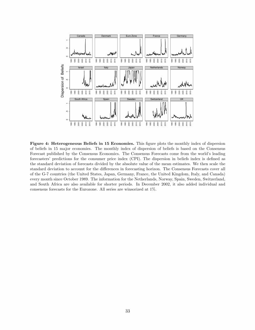
dispersion indices in the 15 economies are plotted in Figure 4. Most of the countries experienced

a surge in the dispersion of beliefs during the crisis in the late 2000s. This is consistent with the

finding of David and Farhat (2018), which documented an elevated level of aggregate dispersion of

beliefs from 2006 to 2016. On average, the level of dispersion of beliefs is the highest in Japan. To

the contrary, both Norway and Denmark have stable and low levels of dispersion of beliefs. The

flat areas in the plot (most noticeable for Japan) are due to winsorization.

[INSERT FIGURE 4 HERE]

4.2 Exchange Rate Changes and Heterogeneous Beliefs

Our empirical tests follow the standard long-horizon predictive regressions (e.g., Fama and French,

1988; Hodrick, 1992; Beber et al., 2010; and Yu, 2013). Specifically, the future changes in foreign

exchange rates are regressed on the proxy of heterogeneity in beliefs and other control variables:

et+3 − et = α+ β(RFt,t+3 −RDt,t+3) + γφt + εt, (29)

where et represents the logarithm of the spot exchange rate at time t against the U.S. dollar. RDt,t+3

(RFt,t+3 ) denotes the domestic (U.S.) interbank rate at time t with a 3-month maturity, and φt is

the dispersion of beliefs.7 Similar to Beber et al. (2010), note that the interest rate differential

is controlled for on the right-hand side. All observations are at monthly frequency. To adjust

for autocorrelated residuals due to overlapping observations, we use Newey-West (1987) standard

errors to correct for the autocorrelation and potential heteroscedasticity.

Table 4 reports the results from the monthly overlapping predictive regression of 3-month

changes in exchange rates on the dispersion of beliefs. The first two columns present the estimated

coefficients of interest rate differential (RF−RD) and the corresponding t-statistics. Consistent with

6For example, the standard deviation for a t-month forecasting horizon (σ) will be re-scaled as σ√

12t

7In the empirical analysis, we treat the U.S. as the “foreign” country, and each of the 15 major economies as the“domestic” country. This is because in our model, money supply is only nontransparent for the domestic country.

22

the previous literature, the coefficients of interest rate differential are largely negative, confirming

the presence of the forward premium puzzle in our sample.

[INSERT TABLE 4 HERE]

The next two columns report the estimated coefficients of dispersion of beliefs (φ) and the

corresponding t-statistics. Our model predicts that future changes in foreign exchange rates are

positively related to the dispersion of beliefs (Hypothesis 1). The evidence is overall supportive.

The coefficient of dispersion of beliefs are positive in 10 out of the 15 economies, and 8 of them are

statistically significant.

Although uncertainty is a prerequisite for the existence of heterogeneous beliefs, these two are

conceptually different. To single out the effect of the dispersion in beliefs, Table 5 re-estimates the

equation (4) after controlling for the uncertainty of the economy, proxied by the VIX index. The

results in Table 5 are largely comparable to those in Table 4. After controlling for the volatility,

the coefficient of dispersion of beliefs are still positive in 10 out of the 15 countries, and 9 of them

are statistically significant.

The evidence in Tables 4 and 5 are based on the absolute level of dispersion of beliefs in each

country. An intuitive alternative is measuring the dispersion of beliefs in each country relative to

the United States. Thus, the second set of tests based on relative dispersion of beliefs are now

presented as additional evidence. The relative dispersion of beliefs (δi) in country i are defined

as δi = log(φi) − log(φus), where φi and φus are the dispersion of beliefs in country i and United

States respectively. Table 6 presents the estimation results. Similar to the previous estimations,

the estimated coefficients of heterogeneous beliefs in most of the countries exhibit have correct signs

and 9 out of 15 are statistically significant.

[INSERT TABLE 5 AND 6 HERE]

4.3 Carry Trade Returns and Heterogeneous Beliefs

Next, we consider the model prediction that the carry trade returns are negatively related to the

dispersion of beliefs. In particular, we regress the 3-month carry trade returns on the dispersion of

beliefs. Table 7 provides evidence supporting this prediction. The regression coefficients for most of

23

the countries have the negative sign, and more than half of them are statistically significant. Table

8 added the volatility (VIX) as a control. Table 9 uses the relative dispersion of beliefs instead

of the absolute dispersion of beliefs in each country. All of the results are largely illustrating a

negative relation between the carry trade returns and dispersion of beliefs.

[INSERT TABLE 7, 8 AND 9 HERE]

A stylized fact of the carry trade strategy is the so-called “up the stairs, down the elevator”

description of the carry trade returns (Boudoukh, Richardson, and Whitelaw, 2016). The carry-

trade returns are periodically hit by the possibility of an abrupt adversarial movement in the

currency market. In our model, the dispersion in beliefs enters the pricing kernel, which determines

how much compensation is required for the potential risk of a sudden loss in value. Consistent with

Beber et al. (2016), our empirical results in section 4.2 and section 4.3 confirm that the dispersion

of beliefs has some predictive power for the considerable and sudden loss in value that a carry trade

strategy suffers from.

Taken together, the empirical evidence is largely supporting our two model predictions. Our

results are robust to an alternative measure of dispersion in beliefs as well as controlling for uncer-

tainty in the economy.

5 Conclusion

Using a two-country model coupled with heterogeneous beliefs, this paper provides a disagreement-

based interpretation of the forward premium puzzle. In our model, the domestic and foreign

investors over- or under-estimate the growth of the domestic money growth rate. In response to a

shock to the domestic money supply, the disagreement between the domestic and foreign investors

moves the foreign exchange rate and interest rate differential in opposite directions. Consequently,

our model could reproduce the rejection of the uncovered interest rate parity. Furthermore, the

time-varying disagreement between investors generates a “trading risk,’ which leads to fluctuations

in exchange rate volatility. In this way, our model could also produce a stochastic volatility of

exchange rate with a comparable magnitude to the actual data.

Our model delivers two testable hypotheses: first, a positive relationship between heterogeneous

24

beliefs and changes in exchange rate; second, a negative relation between carry trade return and

heterogeneous beliefs. Using a monthly index of heterogeneous beliefs based on the Consensus

Forecast in 15 major economies, we confirm the two implications from our model. The empirical

results are still valid after controlling for economic uncertainty, as well as using the relative proxy

of heterogeneity in beliefs.

25

References

[1] Backus, D., S. Foresi, and C. Telmer, 2000. Affine Term Structure Models and the ForwardPremium Anomaly. Journal of Finance 56: 279-304.

[2] Basak, S., 2000. A Model of Dynamic Equilibrium Asset Pricing with Heterogeneous Beliefsand Extraneous Risk. Journal of Economic Dynamics & Control 24: 63-95.

[3] Basak, S., and M. F. Gallmeyer, 1999. Currency Prices, the Nominal Exchange Rate, andSecurity Prices in a Two-Country Dynamic Monetary Equilibrium. Mathematical Finance 9:1-30.

[4] Beber, A., F. Breedon, and A. Buraschi, 2016. Differences in Beliefs and Currency Risk Pre-miums. Journal of Financial Economics 98: 415-38.

[5] Buraschi, A., and A. Jiltsov, 2006. Model Uncertainty and Option Markets with HeterogeneousBeliefs. Journal of Finance 61: 2841-97.

[6] Burnside, C., B. Han, D. Hirshleifer, and T. Y. Wang, 2011. Investor Overconfidence and theForward Premium Puzzle. Review of Economic Studies 78: 1-36.

[7] Cox, J., and C. F. Huang, 1989. Optimal Consumption and Portfolio Policies when AssetPrices Follow a Diffusion Process. Journal of Economic Theory 49: 33-83.

[8] Croitoru, B., and L. Lu, 2015. Asset Pricing in a Monetary Economy with HeterogeneousBeliefs. Management Science 61: 2203-19.

[9] Cuoco, D., and H. He, 1994. Dynamic Equilibrium in Infinite-dimensional Economies withIncomplete Financial Markets. Working paper. University of Pennsylvania.

[10] David, A., 2008. Heterogeneous Beliefs, Speculation, and the Equity Premium. Journal ofFinance 63: 41-83.

[11] David, A., and Farhat, A., 2018. When is the Price of Dispersion Risk Positive? WorkingPaper.

[12] Diether, K. B., C. J. Malloy, and A. Scherbina, 2002. Differences of Opinion and the CrossSection of Stock Returns. Journal of Finance 57: 2113-41.

[13] Dovern, J., U. Fritsche, and J. Slacalek, 2012. Disagreement among Forecasters in G7 Coun-tries. Review of Economics and Statistics 94: 1081-96.

[14] Dumas, B., K. K. Lewis, and E. Osambela, 2017. Differences of Opinion and InternationalEquity Markets. Review of Financial Studies 30: 750-800.

[15] Dumas, B., A. Kurshev, and R. Uppal, 2009. Equilibrium Portfolio Strategies in the Presenceof Sentiment Risk and Excess Volatility. Journal of Finance 64: 579-629.

[16] Fama, F., 1984. Forward and Spot Exchange Rates. Journal of Monetary Economics 14: 319-38.

[17] Gallmeyer, M. F., H. Jhang, and H. Kim, 2016. Value or Growth? Pricing of IdiosyncraticCash-Flow Risk with Heterogeneous Beliefs. Working Paper.

26

[18] Han, B., L. Lu, and Y. Zhou, 2018. Two Trees with Heterogeneous Beliefs: Spillover Effect ofDisagreement. Forthcoming Journal of Financial and Quantitative Analysis.

[19] Hansen, L., and R. Hodrick, 1980. Forward Exchange Rates as Optimal Predictors of FutureSpot Rates: An Economietirc Analysis. Journal of Potical Economy 88: 829-53.

[20] Heyerdahl-Larsen, C., 2014. Asset Prices and Real Exchange Rates with Deep Habits. Reviewof Financial Studies 27: 3280-3317.

[21] Hodric, R. J., 1992. Dividend Yields and Expected Stock Returns: Alternative Procedures forInference and Measurement. Review of Financial Studies 5: 357-86.

[22] Karatzas, I., J. Lehoczky, and S., Shreve, 1990. Existence and Uniqueness of Multi-agent Equi-librium in a Stochastic, Dynamic Consumption/Investment Model. Mathematics of OperationsResearch 15: 80-128.

[23] Li, T., and M. L. Muzere, 2010. Heterogeneity and Volatility Puzzles in International Finance.Journal of Financial and Quantitative Analysis 45: 1485-1516.

[24] Lucas, Jr., R. E., 1982. Interest Rates and Currency Prices in a Two-country World. Journalof Monetary Economy 10: 335-59.

[25] Osambela, E., 2013. Differences of Opinion and Foreign Exchange Markets. Working Paper.

[26] Patton A. J., and A. Timmermann., 2010. Why Do Forecasters Disagree? Lessons from theTerm Structure of Cross-Sectional Dispersion. Journal of Monetary Economy 57: 803-820.

[27] Poon, S. H., and C. W. J. Granger, 2003. Forecasting Volatility in Financial Markets: AReview. Journal of Economic Literature 41: 478-539.

[28] Verdelhan, A., 2010. A Habit-Based Explanation of the Exchange Rate Risk Premium. Journalof Finance 65: 123-46.

[29] Yu, J.F., 2013. A Sentiment-based Explanation of the Forward Premium Puzzle. Journal ofMonetary Economy 60: 474-91.

27

APPENDIX:

Proof of Proposition 1:Each investor maximizes his problem to solve optimal consumption goods and currency holdings.

We insert them into the utility of ”world” representative agent given by:

U(ε, ε∗, qM, q∗M∗/p∗;λ)

= A (λ) + α[βD +

(1− βF

)λ]

log (ε) + α[(

1− βD)

+ βFλ]

log (ε∗)

+ (1− α) [1 + (1− γ)λ] log (qM) + (1− α) γλ[log(q∗

p∗M∗)],

where

A (λ) = α[βD log

(βD

βD+(1−βF )λ

)+(1− βD

)log(

1−βD(1−βD)+βFλ

)]+ αλ

[(1− βF

)log

((1−βF )λ

βD+(1−βF )λt

)+ βF log

(βFλ

(1−βD)+βFλ

)]+ (1− α)

[log(

11+(1−γ)λ

)+ (1− γ)λ log

((1−γ)λ

1+(1−γ)λ

)].

We derive the investor-specific state price density from the first-order conditions of investor’soptimization problem using domestic consumption goods as a numeraire (e.g., Buraschi, Trojani,and Vedolin, 2014). Applying Ito’s lemma to investor-specific state price density, we can calculatethe market price of risk. The nominal interest rates can be calculated as

Rt =UM,tUε,t

= ∂Ut∂(qM)t

1∂Ut∂εt

= 1−αα

1+(1−γ)λtβD+(1−βF )λt

εtqtMt

,

R∗t =UM∗,tUε∗,t

= ∂Ut

∂

(q∗tp∗tM∗t

) 1∂Ut∂ε∗t

= 1−αα

γλt(1−βD)+βFλt

p∗t ε∗t

q∗tM∗t.

In the following, we derive the prices of foreign consumption goods, domestic currency, andforeign currency relative to the price of domestic consumption goods. First, the price of foreignconsumption goods relative to the price of domestic consumption goods is

p∗t =Uε∗,tUε,t

=(1−βD)+βFλt

βD+(1−βF )λtεtε∗t,

Next, we calculate the price of domestic currency relative to the price of domestic consumptiongoods.

Ms = Mt expµDM (s− t) + σMε (ωε,s − ωε,t) + σMε∗ (ωε∗,s − ωε∗,t) + σMM

(ωDM,s − ωDM,t

),

λs = λt exp−1

2 µ2M (s− t)− µM

(ωDM,s − ωDM,t

).

We have

EDt

[1Ms

]= 1

MtEDt

[exp

−µDM (s− t)− σMε (ωε,s − ωε,t)− σMε∗ (ωε∗,s − ωε∗,t)− σMM

(ωDM,s − ωDM,t

)]= 1

Mtexp

(12σ

2M − µDM

)(s− t)

,

where σ2M = σ2

Mε + σ2Mε∗ + σ2

MM . Thus,∫ Tt E

Dt

[1Ms

]ds = 1

Mt

exp(

12σ

2M−µ

DM

)(T−t)

−1

12σ

2M−µ

DM

.

28

Therefore, we have

EDt

[λsMs

]= λt

MtEDt

[exp

−1

2 µ2M (s− t)− µDM (s− t)− σMε (ωε,s − ωε,t)

−σMε∗ (ωε∗,s − ωε∗,t)− (µM + σMM )(ωDM,s − ωDM,t

) ]= λt

Mtexp

(12σ

2M − µFM

)(s− t)

.∫ T

t EDt

[λsMs

]ds = λt

Mt

exp(

12σ

2M−µ

FM

)(T−t)

−1

12σ

2M−µ

FM

.

Therefore, the price of domestic currency relative to the price of domestic consumption goods is

qt = 1ξDtEDt

[∫ Tt ξ

Ds Rsqsds

]= (1−α)εt

α[βD+(1−βF )λt]EDt

[∫ Tt

1+(1−γ)λsMs

ds]

= (1−α)εtα[βD+(1−βF )λt]

[∫ Tt E

Dt

[1Ms

]ds+ (1− γ)

∫ Tt E

Dt

[λsMs

]ds]

= (1−α)εtα[βD+(1−βF )λt]

[1Mt

exp(

12σ

2M−µ

DM

)(T−t)

−1

12σ

2M−µ

DM

+ (1− γ) λtMt

exp(

12σ

2M−µ

FM

)(T−t)

−1

12σ

2M−µ

FM

]=

(1−α)[GDt +(1−γ)λtGFt ]α[βD+(1−βF )λt]

εtMt,

where Git =exp(

12σ

2M−µ

iM

)(T−t)

−1

12σ

2M−µ

iM

(i = D,F ).

Finally, we calculate the price of foreign currency relative to the price of domestic consumptiongoods.

M∗s = M∗t exp µM∗ (s− t) + σM∗ε∗ (ωε∗,s − ωε∗,t) + σM∗M∗ (ωM∗,s − ωM∗,t) ,

We have∫ Tt E

Dt

[1M∗s

]ds = 1

M∗t

exp(

12σ

2M∗−µM∗

)(T−t)

−1

12σ

2M∗−µM∗

, where σ2M∗ = σ2

M∗ε∗ + σ2M∗M∗ .

q∗t = 1ξDtEDt

[∫ Tt ξ

Ds R∗sq∗sds]

= (1−α)εtα[βD+(1−βF )λt]

EDt

[∫ TtγλsM∗s

ds]

= γ(1−α)εtα[βD+(1−βF )λt]

∫ Tt E

Dt

[λsM∗s

]ds = γ(1−α)εt

α[βD+(1−βF )λt]

∫ Tt E

Dt

[1M∗s

]EDt [λs] ds

= (1−α)γHtλtα[βD+(1−βF )λt]

εtM∗t

,

where Ht =exp(

12σ

2M∗−µM∗

)(T−t)

−1

12σ

2M∗−µM∗

.

Proof of Proposition 2:The nominal foreign exchange rate is given by

et = qtq∗t

=GDt +(1−γ)λtGFt

γHtλt

M∗tMt.

Applying Ito’s lemma to nominal foreign exchange rate, et, we can derive its drift and diffusioncoefficients.

29

Proof of Proposition 3:The prices of domestic and foreign stocks are given by

St = 1ξDtEDt

[∫ Tt ξ

Ds εsds

]= (T − t) εt,

S∗t = 1ξDtEDt

[∫ Tt ξ

Ds p∗sε∗sds]

=(1−βD)+βFλt

βD+(1−βF )λtSt =

(1−βD)+βFλt

βD+(1−βF )λt(T − t) εt = (T − t) p∗t ε∗t .

Applying Ito’s lemma to the prices of domestic and foreign stocks, respectively, we can calculatetheir expected stock returns and diffusion coefficients.

30

0 0.05 0.1 0.15 0.2 0.250

0.02

0.04

0.06

0.08

0.1

0.12

µM

Exchange R

ate

Vola

tilit

yHeterogeneous Beliefs and Exchange Rate Volatility

(a)

1985 1990 1995 2000 2005 2010 2015 20200

0.1

0.2

0.3

0.4

0.5

0.6

0.7

Date

Exchange R

ate

Vola

tilit

y

Actual and Model Generated Exchange Rate Volatility

Model Generated

Actual

(b)

Figure 1: Exchange Rate Volatility. This figure examines the volatility of the exchange rate generatedby our model. To illustrate the model implied relation between heterogeneous beliefs and exchange ratevolatility, we conduct a set of simulations using model parameters as those in Table 1, while manually adjustthe level of heterogeneous beliefs. For each value of µM = (µD

M − µFM )/σMM , we simulate 10,000 paths

and compute the average exchange rate volatility. Plot (a) shows the volatility of the nominal exchangerate in the baseline calibration against the dispersion of beliefs, measured by differences in beliefs betweendomestic and foreign investors (µM ). Using the actual proxy for heterogeneous beliefs in the U.S. and theU.K., we compute the model generated exchange rate volatility. The proxy for heterogeneous beliefs is amonthly index of dispersion of beliefs using the Consensus Forecast published by the Consensus Economics.Figure 1(b) compares the model generated exchange rate volatility and the actual monthly volatility of theUSD/GBP exchange rate. The volatility of the USD/GBP exchange rate is computed using daily currencyreturns in each month.

31

0 0.05 0.1 0.15 0.2 0.25-3

-2

-1

0

1

2

3

µM

Ave

rage

Carr

y T

rad

e R

etu

rn (

%)

Heterogeneous Beliefs and Carry Trade Return

Figure 2: Heterogeneous Beliefs and Carry Trade Returns. This figure plots the model implied relationbetween heterogeneous beliefs and average carry trade return. We conduct a set of simulations using model parametersas those in Table 1, while manually adjust the heterogeneous beliefs. For each value of µM , we simulate 10,000 pathsand compute the average carry trade return as in equation (23).

0 0.05 0.1 0.15 0.2 0.25-4

-3

-2

-1

0

1

2

µM

et+

1 -

et (

%)

Heterogeneous Beliefs and Changes in Exchange Rate

(a) Changes in Exchange Rate

0 0.05 0.1 0.15 0.2 0.25

-1

-0.8

-0.6

-0.4

-0.2

µM

RF -

RD

(%

)

Heterogeneous Beliefs and Forward Premium

(b) Forward Premium

Figure 3: Carry Trade Return Decomposition. This figure decomposes carry returns into returns generated

by the interest rate differentials and the returns generated by exchange-rate appreciation/depreciation. We conduct

a set of simulations using model parameters as those in Table 1, while manually adjust the level of heterogeneous

beliefs. For each value of µM , we simulate 10,000 paths and compute the average returns of exchange rate (et+1 − et)and the interest rate differentials between foreign and domestic interest rate (RFt −RDt ), where et is the natural log

of exchange rate at time t, RFt and RDt are the domestic and foreign interest rate at time t, respectively.

32

0.5

10

.51

0.5

1

19

90

19

95

20

00

20

05

20

10

20

15

19

90

19

95

20

00

20

05

20

10

20

15

19

90

19

95

20

00

20

05

20

10

20

15

19

90

19

95

20

00

20

05

20

10

20

15

19

90

19

95

20

00

20

05

20

10

20

15

19

90

19

95

20

00

20

05

20

10

20

15

19

90

19

95

20

00

20

05

20

10

20

15

19

90

19

95

20

00

20

05

20

10

20

15

19

90

19

95

20

00

20

05

20

10

20

15

19

90

19

95

20

00

20

05

20

10

20

15

19

90

19

95

20

00

20

05

20

10

20

15

19

90

19

95

20

00

20

05

20

10

20

15

19

90

19

95

20

00

20

05

20

10

20

15

19

90

19

95

20

00

20

05

20

10

20

15

19

90

19

95

20

00

20

05

20

10

20

15

Canada Denmark Euro Zone France Germany

Israel Italy Japan Netherlands Norway

South Africa Spain Sweden Switzerland UK

Dis

pers

ion o

f B

elie

fs

Figure 4: Heterogeneous Beliefs in 15 Economies. This figure plots the monthly index of dispersionof beliefs in 15 major economies. The monthly index of dispersion of beliefs is based on the ConsensusForecast published by the Consensus Economics. The Consensus Forecasts come from the world’s leadingforecasters’ predictions for the consumer price index (CPI). The dispersion in beliefs index is defined asthe standard deviation of forecasts divided by the absolute value of the mean estimates. We then scale thestandard deviation to account for the differences in forecasting horizon. The Consensus Forecasts cover allof the G-7 countries (the United States, Japan, Germany, France, the United Kingdom, Italy, and Canada)every month since October 1989. The information for the Netherlands, Norway, Spain, Sweden, Switzerland,and South Africa are also available for shorter periods. In December 2002, it also added individual andconsensus forecasts for the Eurozone. All series are winsorized at 1%.

33

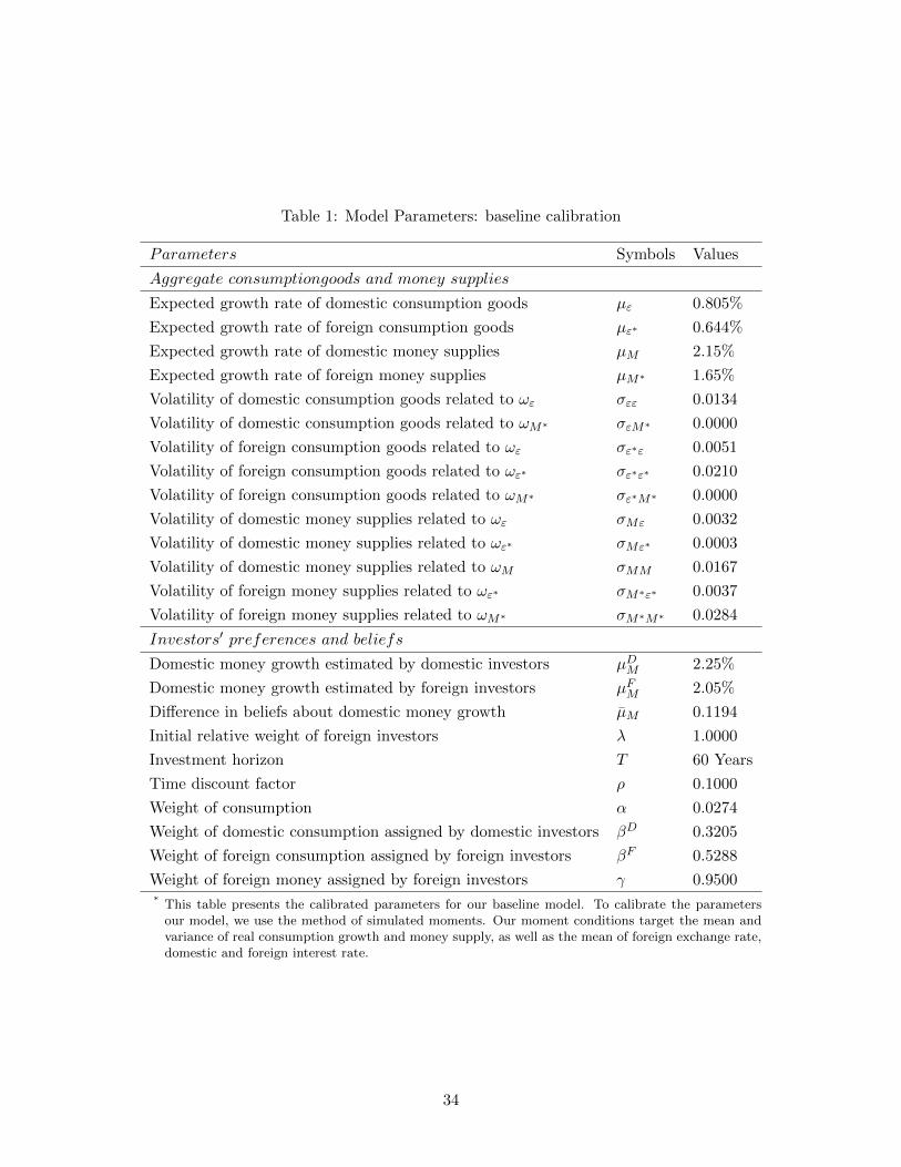
Table 1: Model Parameters: baseline calibration

Parameters Symbols Values

Aggregate consumptiongoods and money supplies

Expected growth rate of domestic consumption goods µε 0.805%

Expected growth rate of foreign consumption goods µε∗ 0.644%

Expected growth rate of domestic money supplies µM 2.15%

Expected growth rate of foreign money supplies µM∗ 1.65%

Volatility of domestic consumption goods related to ωε σεε 0.0134

Volatility of domestic consumption goods related to ωM∗ σεM∗ 0.0000

Volatility of foreign consumption goods related to ωε σε∗ε 0.0051

Volatility of foreign consumption goods related to ωε∗ σε∗ε∗ 0.0210

Volatility of foreign consumption goods related to ωM∗ σε∗M∗ 0.0000

Volatility of domestic money supplies related to ωε σMε 0.0032

Volatility of domestic money supplies related to ωε∗ σMε∗ 0.0003

Volatility of domestic money supplies related to ωM σMM 0.0167

Volatility of foreign money supplies related to ωε∗ σM∗ε∗ 0.0037

Volatility of foreign money supplies related to ωM∗ σM∗M∗ 0.0284

Investors′ preferences and beliefs

Domestic money growth estimated by domestic investors µDM 2.25%

Domestic money growth estimated by foreign investors µFM 2.05%

Difference in beliefs about domestic money growth µM 0.1194

Initial relative weight of foreign investors λ 1.0000

Investment horizon T 60 Years

Time discount factor ρ 0.1000

Weight of consumption α 0.0274

Weight of domestic consumption assigned by domestic investors βD 0.3205

Weight of foreign consumption assigned by foreign investors βF 0.5288

Weight of foreign money assigned by foreign investors γ 0.9500* This table presents the calibrated parameters for our baseline model. To calibrate the parameters

our model, we use the method of simulated moments. Our moment conditions target the mean andvariance of real consumption growth and money supply, as well as the mean of foreign exchange rate,domestic and foreign interest rate.

34

Table 2: Moments on Key Variables

Actual Model

Target moment conditions

mean of domestic consumption growth rate 0.805% 0.81%

mean of foreign consumption growth rate 0.644% 0.64%

mean of domestic money supply growth rate 1.654% 1.66%

mean of foreign money supply growth rate 2.155% 2.15%

volatility of domestic consumption growth rate 0.680% 0.67%

volatility of foreign consumption growth rate 1.059% 1.08%

volatility of domestic money supply growth rate 0.853% 0.85%

volatility of foreign money supply growth rate 1.504% 1.43%

mean of domestic interest rate 4.50% 3.91%

mean of interest rate differential 2.10% 1.08%

mean of the foreign exchange rate 0.495 0.56

Other moment conditions

volatility of the foreign exchange rate 3.978% 6.78%

volatility of domestic nominal interest rate (×10−4) 0.786 0.84

volatility of foreign nominal interest rate (×10−4) 0.916 0.96

volatility of interest rate differential (×10−4) 1.065 1.46

correlation of domestic and foreign money supply 0.258 0.12

correlation of domestic and foreign interest rate 0.872 0.98

correlation of domestic and foreign consumption 0.236 0.24

mean of domestic excess return 0.066 0.02

mean of foreign excess return 0.048 0.02

volatility of domestic stock return 0.155 0.01

volatility of foreign stock return 0.198 0.02* This table reports the unconditional moments of our baseline calibration. Using the calibrated param-

eters in Table 1, we simulate the model across 10,000 paths of 160 quarterly observations each. Wereport the unconditional moments of the actual data, as well as the average moments obtained fromour simulation. The domestic country is the United States, and the foreign country is United King-dom. Our sample of actual data contains quarterly observations from 1955 until 2016 in the UnitedStates and United Kingdom obtained from Federal Reserve Economic Data (FRED) database. Theinterest rate is the 3-month inter-bank rate. The money supply is the M2 money supply in the US,and M4 money supply in the UK. The stock return is the S&P 500 total return index in the USand the FTSE 100 index return in the UK. The foreign exchange rate is measured by the averageUSD/GBP rate in each quarter.

35

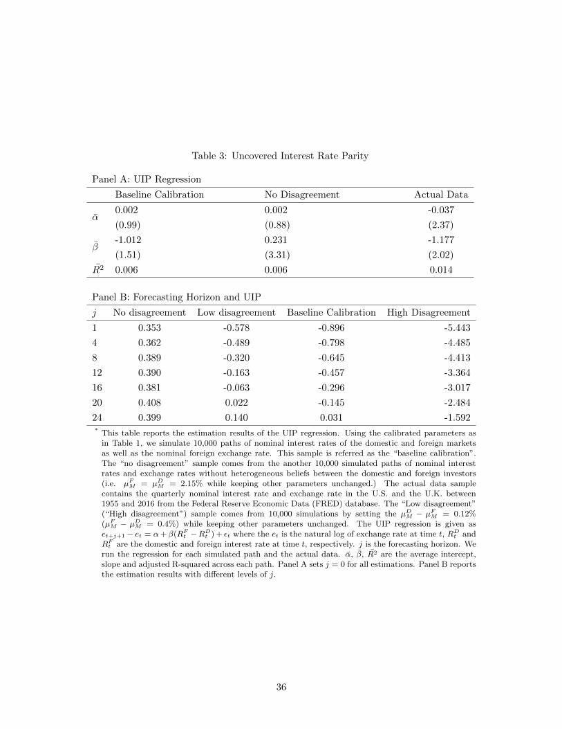
Table 3: Uncovered Interest Rate Parity

Panel A: UIP Regression

Baseline Calibration No Disagreement Actual Data

α0.002

(0.99)

0.002

(0.88)

-0.037

(2.37)

β-1.012

(1.51)

0.231

(3.31)

-1.177

(2.02)

R2 0.006 0.006 0.014

Panel B: Forecasting Horizon and UIP

j No disagreement Low disagreement Baseline Calibration High Disagreement

1 0.353 -0.578 -0.896 -5.443

4 0.362 -0.489 -0.798 -4.485

8 0.389 -0.320 -0.645 -4.413

12 0.390 -0.163 -0.457 -3.364

16 0.381 -0.063 -0.296 -3.017

20 0.408 0.022 -0.145 -2.484

24 0.399 0.140 0.031 -1.592* This table reports the estimation results of the UIP regression. Using the calibrated parameters as

in Table 1, we simulate 10,000 paths of nominal interest rates of the domestic and foreign marketsas well as the nominal foreign exchange rate. This sample is referred as the “baseline calibration”.The “no disagreement” sample comes from the another 10,000 simulated paths of nominal interestrates and exchange rates without heterogeneous beliefs between the domestic and foreign investors(i.e. µFM = µDM = 2.15% while keeping other parameters unchanged.) The actual data samplecontains the quarterly nominal interest rate and exchange rate in the U.S. and the U.K. between1955 and 2016 from the Federal Reserve Economic Data (FRED) database. The “Low disagreement”(“High disagreement”) sample comes from 10,000 simulations by setting the µDM − µFM = 0.12%(µFM − µDM = 0.4%) while keeping other parameters unchanged. The UIP regression is given aset+j+1 − et = α+ β(RFt −RDt ) + εt where the et is the natural log of exchange rate at time t, RDt andRFt are the domestic and foreign interest rate at time t, respectively. j is the forecasting horizon. Werun the regression for each simulated path and the actual data. α, β, R2 are the average intercept,slope and adjusted R-squared across each path. Panel A sets j = 0 for all estimations. Panel B reportsthe estimation results with different levels of j.

36

Table 4: Exchange rate changes and Heterogeneous Beliefs

RF −RD t-stats φt t-stats R2

Canada -0.315 (-0.16) 0.089*** (3.45) 0.036

Denmark -1.438*** (-2.90) 0.118 (1.27) 0.060

Euro Zone -1.102* (-2.13) -0.015 (-0.51) 0.028

France -1.413 (-0.75) -0.003 (-0.14) 0.002

Germany -2.444 (-1.18) 0.058* (1.72) 0.011

Israel -1.653** (-2.41) -0.001 (-0.06) 0.065

Italy -4.987*** (-3.44) 0.058*** (2.85) 0.048

Japan -2.946 (-1.38) -0.009 (-0.80) 0.012

Netherlands -7.461** (-2.29) 0.001 (0.03) 0.021

Norway 1.061 (0.34) 0.207*** (3.34) 0.049

South Africa -1.609** (-2.54) 0.300** (2.36) 0.055

Spain -2.060 (-0.70) 0.025* (1.67) 0.011

Sweden -6.692* (-2.23) -0.014 (-0.71) 0.021

Switzerland -8.353** (-2.23) 0.024* (1.69) 0.025

United Kingdom -1.327 (-0.67) 0.052** (2.43) 0.020* This table reports the estimation results of the standard long-horizon predictive regressions. Specif-

ically, the future changes in foreign exchange rates are regressed on the proxy of heterogeneity inbeliefs and other control variables: et+3 − et = α+ β(RFt,t+3 −RDt,t+3) + γφt + εt, where et representsthe logarithm of the spot exchange rate at time t against the U.S. dollar. RDt,t+3 (RFt,t+3 ) denotesthe domestic (U.S.) interbank rate at time t with a 3-month maturity, and φt is the dispersion ofbeliefs. The sample period is October 1989 to December 2016. All observations are at monthly fre-quency. The information on exchange rate and interest rate is from the Federal Reserve EconomicData (FRED) database. The proxy of dispersion of beliefs is from the Consensus Forecast publishedby the Consensus Economics. Standard errors are adjusted as in Newey-West (1987). ***, **, and *indicate significance at 1%, 5%, and 10% levels, respectively.

37

Table 5: Exchange rate changes, Heterogeneous Beliefs, and VIX

RF −RD t-stats φt t-stats VIX t-stats R2

Canada -0.566 (-0.29) 0.076** (2.90) 0.066** (2.18) 0.050

Denmark -3.460*** (-5.63) 0.104** (2.22) 0.339*** (4.94) 0.020

Euro Zone -2.337*** (-3.97) -0.018 (-0.65) 0.228*** (3.91) 0.011

France -1.470 (-0.79) -0.006 (-0.28) 0.045 (1.06) 0.005

Germany -2.350 (-1.14) 0.051* (1.71) 0.029 (0.67) 0.012

Israel -1.678** (-2.43) -0.002 (-0.13) -0.023 (-0.47) 0.066

Italy -4.744** (-3.22) 0.055** (2.63) 0.034 (0.78) 0.050

Japan -3.354* (-1.77) -0.009 (-0.80) 0.080* (1.74) 0.021

Netherlands -5.664* (-1.69) 0.011 (0.31) 0.055 (1.26) 0.025

Norway 6.994 (0.93) 0.221*** (3.65) 0.148** (2.51) 0.082

South Africa -4.885 (-0.65) 0.234* (1.84) 0.248** (2.61) 0.101

Spain -1.376 (-0.47) 0.023* (1.79) 0.059 (1.42) 0.018

Sweden -6.261* (-2.08) -0.012 (-0.61) 0.049 (1.05) 0.024

Switzerland -7.538* (-2.01) 0.020* (1.68) 0.038 (0.89) 0.026

U.K. -1.266 (-0.64) 0.0569* (2.56) -0.0293 (-0.70) 0.022* This table reports the estimation results of the standard long-horizon predictive regressions. Specifically, the

future changes in foreign exchange rates are regressed on the proxy of heterogeneity in beliefs and other controlvariables: et+3 − et = α + β(RFt,t+3 − RDt,t+3) + γφt + VIX + εt, where et represents the logarithm of the spotexchange rate at time t against the U.S. dollar. RDt,t+3 (RFt,t+3 ) denotes the domestic (U.S.) interbank rate attime t with a 3-month maturity, and φt is the dispersion of beliefs. VIX is the CBOE Volatility Index. Thesample period is October 1989 to December 2016. All observations are at monthly frequency. The informationon exchange rate and interest rate is from the Federal Reserve Economic Data (FRED) database. The proxy ofdispersion of beliefs is from the Consensus Forecast published by the Consensus Economics. Standard errors areadjusted as in Newey-West (1987). ***, **, and * indicate significance at 1%, 5%, and 10% levels, respectively.

38

Table 6: Exchange rate changes, Relative Heterogeneous Beliefs, and VIX

RF −RD t-stats δt t-stats VIX t-stats R2

Canada 0.383 (0.19) 0.046 (0.01) -0.018*** (-2.73) 0.025

Denmark -3.347*** (-5.52) 0.064* (1.71) -0.067*** (-4.94) 0.019

Euro Zone -2.433*** (-4.19) 0.020* (2.38) -0.045*** (-3.87) 0.013

France 0.570 (0.29) 0.024** (3.00) -0.009 (-0.98) 0.032

Germany -2.511 (-1.17) -0.039 (-0.45) -0.010 (-1.09) 0.007

Israel -2.403** (-3.29) 0.013* (1.75) 0.035** (2.22) 0.082

Italy -4.588** (-3.24) 0.024*** (4.19) -0.005 (-0.50) 0.080

Japan -3.867 (-1.54) 0.049 (0.07) -0.006 (-0.46) 0.019

Netherlands -5.816* (-1.80) 0.065 (0.92) -0.010 (-1.00) 0.028

Norway 6.228* (1.69) 0.022** (2.08) -0.030* (-2.46) 0.045

South Africa -3.644 (-0.46) -0.019 (-1.33) -0.081*** (-2.95) 0.090

Spain -1.520 (-0.52) 0.014** (2.65) -0.014 (-1.49) 0.036

Sweden -4.817 (-1.56) 0.013** (1.97) -0.004 (-0.39) 0.037

Switzerland -5.762* (-1.70) 0.012* (1.87) 0.017 (1.29) 0.033

U.K. 1.545 (0.76) 0.014 (0.20) -0.087 (-0.10) 0.002* This table reports the estimation results of the standard long-horizon predictive regressions. Specifically, the

future changes in foreign exchange rates are regressed on the proxy of relative heterogeneity in beliefs and othercontrol variables: et+3 − et = α+ β(RFt,t+3 − RDt,t+3) + γδt + VIX + εt, where et represents the logarithm of thespot exchange rate at time t against the U.S. dollar. RDt,t+3 (RFt,t+3 ) denotes the domestic (U.S.) interbank rateat time t with a 3-month maturity, and δt is the relative dispersion of beliefs. The relative dispersion of beliefs(δi) in country i are defined as δi = log(φi) − log(φus), where φi and φus are the dispersion of beliefs in countryi and United States respectively. VIX is the CBOE Volatility Index. The sample period is October 1989 toDecember 2016. All observations are at monthly frequency. The information on exchange rate, interest rate andVIX is from the Federal Reserve Economic Data (FRED) database. The proxy of dispersion of beliefs is fromthe Consensus Forecast published by the Consensus Economics. Standard errors are adjusted as in Newey-West(1987). ***, **, and * indicate significance at 1%, 5%, and 10% levels, respectively.

39

Table 7: Carry Trade Returns and Heterogeneous Beliefs

φt t-stats R2

Canada -0.0859*** (-3.39) 0.034

Denmark -0.0462 (-0.51) 0.002

Euro Zone 0.0161 (0.54) 0.002

France 0.00753 (0.33) 0.010

Germany -0.0553* (-1.75) 0.006

Israel -0.0311* (-1.76) 0.022

Italy -0.0459** (-2.26) 0.015

Japan -0.0174* (-1.70) 0.008

Netherlands -0.0258 (-0.76) 0.002

Norway -0.207*** (-3.35) 0.049

South Africa -0.125* (-1.81) 0.009

Spain -0.0242* (-1.63) 0.009

Sweden -0.0164 (-0.82) 0.003

Switzerland 0.00929 (0.69) 0.002

United Kingdom -0.0523** (-2.44) 0.018* This table reports results of regressing 3-month carry trade returns on heterogeneous beliefs(φt).

The carry trade returns from investing in the currency market are given as: CTRt+3 = RFt,t+3 −RDt,t+3 − (et+3 − et), where et represents the logarithm of the spot exchange rate at time t againstthe U.S. dollar. RDt,t+3 (RFt,t+3 ) denotes the domestic (U.S.) interbank rate at time t with a 3-monthmaturity. The sample period is October 1989 to December 2016. All observations are at monthlyfrequency. The information on exchange rate and interest rate is from the Federal Reserve EconomicData (FRED) database. The proxy of dispersion of beliefs is from the Consensus Forecast publishedby the Consensus Economics. Standard errors are adjusted as in Newey-West (1987). ***, **, and *indicate significance at 1%, 5%, and 10% levels, respectively.

40

Table 8: Carry Trade Returns, Heterogeneous Beliefs, and VIX

φt t-stats VIX t(VIX) R2

Canada -0.072*** (-2.80) -0.064* (-2.14) 0.048

Denmark -0.014 (-0.15) -0.089 (-1.58) 0.020

Euro Zone 0.018 (0.62) -0.109* (-2.13) 0.029

France 0.010 (0.46) -0.041 (-0.97) 0.003

Germany -0.049* (-1.76) -0.027 (-0.62) 0.008

Israel -0.030* (-1.70) 0.014 (0.30) 0.023

Italy -0.041** (-2.03) -0.058 (-1.32) 0.021

Japan -0.018 (-1.66) -0.071 (-1.54) 0.015

Netherlands -0.032 (-0.97) -0.081 (-1.91) 0.016

Norway -0.216*** (-3.55) -0.095 (-1.91) 0.070

South Africa -0.182* (-1.68) -0.290*** (-3.72) 0.100

Spain -0.022* (-1.75) -0.062 (-1.49) 0.017

Sweden 0.014 (0.70) -0.054 (-1.14) 0.007

Switzerland 0.006 (0.46) -0.047 (-1.09) 0.007

U.K. -0.057** (-2.58) 0.029 (0.71) 0.020* This table reports results of regressing 3-month carry trade returns on heterogeneous beliefs(φt),

and VIX. The carry trade returns from investing in the currency market are given as: CTRt+3 =RFt,t+3 − RDt,t+3 − (et+3 − et), where et represents the logarithm of the spot exchange rate at time tagainst the U.S. dollar. RDt,t+3 (RFt,t+3 ) denotes the domestic (U.S.) interbank rate at time t with a 3-month maturity. VIX is the CBOE Volatility Index. The sample period is October 1989 to December2016. All observations are at monthly frequency. The information on exchange rate, interest rate,and VIX is from the Federal Reserve Economic Data (FRED) database. The proxy of dispersion ofbeliefs is from the Consensus Forecast published by the Consensus Economics. Standard errors areadjusted as in Newey-West (1987). ***, **, and * indicate significance at 1%, 5%, and 10% levels,respectively.

41

Table 9: Carry Trade Returns, Relative Heterogeneous Beliefs, and VIX

δt t-stats VIX t(VIX) R2

Canada -0.035** (-2.08) -0.084** (-2.79) 0.024

Denmark -0.003 (-0.31) -0.084 (-1.45) 0.020

Euro Zone -0.018** (-2.01) -0.075 (-1.43) 0.050

France -0.025** (-3.31) -0.026 (-0.64) 0.035

Germany 0.022 (0.03) -0.041 (-0.96) 0.003

Israel 0.005 (0.86) 0.306 (0.05) 0.007

Italy -0.021*** (-3.84) -0.022 (-0.49) 0.051

Japan -0.008* (-1.69) -0.056 (-1.22) 0.014

Netherlands -0.007 (-1.05) -0.058 (-1.27) 0.017

Norway -0.022* (-2.09) -0.136* (-2.51) 0.035

South Africa 0.014 (1.21) -0.317*** (-3.68) 0.092

Spain -0.013*** (-2.61) -0.042 (-1.00) 0.034

Sweden -0.017** (-2.51) -0.021 (-0.44) 0.029

Switzerland -0.011* (-1.74) -0.022 (-0.48) 0.020

U.K. -0.002 (-0.25) 0.304 (0.07) 0.001* This table reports results of regressing 3-month carry trade returns on relative heterogeneous

beliefs(δt), and VIX. The carry trade returns from investing in the currency market are given as:CTRt+3 = RFt,t+3 − RDt,t+3 − (et+3 − et), where et represents the logarithm of the spot exchangerate at time t against the U.S. dollar. RDt,t+3 (RFt,t+3 ) denotes the domestic (U.S.) interbank rateat time t with a 3-month maturity. The relative dispersion of beliefs (δi) in country i are defined asδi = log(φi) − log(φus), where φi and φus are the dispersion of beliefs in country i and United Statesrespectively. VIX is the CBOE Volatility Index. The sample period is October 1989 to December2016. All observations are at monthly frequency. The information on exchange rate, interest rate,and VIX is from the Federal Reserve Economic Data (FRED) database. The proxy of dispersion ofbeliefs is from the Consensus Forecast published by the Consensus Economics. Standard errors areadjusted as in Newey-West (1987). ***, **, and * indicate significance at 1%, 5%, and 10% levels,respectively.

42