Document de travail  

HETEROGENEITY AND THE DISTANCE PUZZLE

Elizaveta Archanskaia OFCE-Sciences-Po

Guillaume Daudin EQUIPPE/Lille-I & OFCE-Sciences-Po

 

 

 

 

 

2012

- 17

/ M

ay 2

01

2

 

Heterogeneity and the Distance Puzzle∗

Elizaveta Archanskaia† Guillaume Daudin‡

May 2012

Preliminary version - Comments welcome

Abstract

This paper shows that reduced heterogeneity of exporter-specific goods can provide adirect explanation of the distance puzzle. Using COMTRADE 4-digit bilateral trade datawe find that the elasticity of trade to distance has increased by 8% from 1962 to 2009.Theoretical foundations of the gravity equation indicate that the distance coefficient is theproduct of the elasticity of trade costs to distance and a measure of heterogeneity, e.g.the substitution elasticity between exporter-specific goods in the Armington framework.This parameter has increased by 13% from 1962 to 2009. The evolution of the distancecoefficient is thus compatible with a 4% reduction in the elasticity of trade costs to distance.

Keywords: gravity equation, distance puzzle, trade elasticity, trade costs

JEL codes: F15, N70

∗This paper has greatly benefited from helpful discussions with Lorenzo Caliendo, Thomas Chaney, Anne-Célia Disdier, Lionel Fontagné, Raphaël Franck, Guillaume Gaulier, Samuel Kortum, Jacques Le Cacheux, Fer-nando Parro, and suggestions by seminar participants at SciencesPo, ADRES, AFSE, ETSG, the InternationalTrade Working Group at the University of Chicago, and the international workshop on the Economics of GlobalInteractions (Bari). We thank Christian Broda, Natalie Chen, Dennis Novy, and David E. Weinstein for giving usaccess to their programs. The usual disclaimers apply.

†SciencesPo/OFCE‡Corrsponding author. Lille-I/EQUIPPE and Sciences Po/OFCE. Email:gdaudin@mac.com

1

Introduction

The estimated effect of distance in gravity equations has remained stable, or even slightly

increased, in the past 50 years.1 This is the “distance puzzle”, as the common opinion is that

technological developments in transports, e.g. the airplane and the container, had contributed to

the “death of distance” (Cairncross (1997); Levinson (2006); Friedman (2007)).

Recent work on the distance puzzle has gone in two directions. Following Santos Silva and

Tenreyro, one strand of the literature has sought to correct the estimation method using non

linear estimators (Santos Silva and Tenreyro (2006); Coe et al. (2007); Bosquet and Boulhol

(2009). See §I.2 for a discussion). The canonical log-linear estimation does not generally pro-

vide consistent coefficient estimates if the trade equation in levels is subject to heteroskedastic-

ity. Furthermore, the log-linear estimation strategy suffers from sample selection bias because

it cannot take into account nil trade flows. The growth of trade has been both intensive, in the

sense that the volume of trade of established trade relations has increased, and extensive, in

the sense that new trade relations have been established (Helpman et al. (2008); Baldwin and

Harrigan (2007)). Taking zeros into account might change the evolution of the distance coeffi-

cient if new trade relations have in priority been established between distant partners. Using a

non-linear estimator, Bosquet and Boulhol (2009) find that the distance elasticity of trade has

been stable within the .6-.75 range between 1948 and 2006. Coe et al. (2007) find that it has

decreased from 0.5 to 0.3 in 1975-2000.

The other strand of the literature has argued that there is no puzzle, as there are theoretical

and empirical explanations of a non decreasing distance elasticity of trade (Bosquet and Boulhol

(2009); Duranton and Storper (2008); Buch et al. (2004)). Firstly, a composition effect might

explain a non decreasing distance coefficient. It might be that the composition of traded goods

has changed toward goods which are either less transportable or which consumption is more

sensible to trade costs. Theoretically, Duranton and Storper (2008) show how falling transport

costs can induce firms into trading goods with higher transaction costs, leading to an increasing

distance sensitivity of trade. Empirically, Berthelon and Freund (2008) test the impact of the

changing composition of world trade between 1985 and 2005 on the distance coefficient, but

1 Disdier and Head (2008) find that distance impedes trade by 37% more since 1990 than it did from 1870 to1969 Berthelon and Freund (2008) find that the distance coefficient has increased by 10% in absolute valueover the period 1985-2005. See also Bosquet and Boulhol (2009); Coe et al. (2007); Combes et al. (2006);Brun et al. (2005); Buch et al. (2004).

2

find that it has had a negligible effect.2 Using a log-linear estimation strategy, Brun et al.

(2005) and Márquez-Ramos et al. (2007) find decreasing distance elasticities once the sample

is restricted to developed countries.

Secondly, it is not certain that transport costs have declined relative to the price of traded

goods (Hummels (1999); Daudin (2003, 2005); Hummels (2007)). Furthermore, it might be

the case that other distance-related components of trade costs, such as delays, have a growing

importance (Hummels and Schaur (2012); Hummels (2001)).

Thirdly, the value of the distance coefficient in theoretically derived gravity models of trade

is not directly related to the level of trade costs.3 It is the product of two elasticities: the

elasticity of trade flows to distance-related trade costs, and the elasticity of trade costs to dis-

tance. Whether transport costs have declined or increased, the crucial question for the evolution

of the coefficient is whether non-distance dependent transport costs, such as loading costs at

ports, have declined relatively to distance-dependent transport costs, such as fuel costs (Feyrer

(2009)).

The discussion on the distance puzzle in this second strand of the literature has been mainly

concerned with the evolution of the elasticity of trade costs to distance. One should look as

well at the elasticity of trade flows to trade costs. Following ?, we refer to this parameter as

the ‘trade elasticity’. The structural interpretation of the trade elasticity depends on the micro

foundations used to derive the gravity equation: in the canonical models this paper builds on, it

corresponds alternatively to the dispersion in productive efficiency across sectors, to elasticities

of substitution between country-composite goods , or to the intrasectoral dispersion in firm

productivity. In all cases, the trade elasticity is inversely linked to the measure of heterogeneity

in some dimension.

For example, since the 1960s, a number of countries have demonstrated their ability to

produce the same set of goods as developed countries. This may have resulted in more uni-

formity in country-specific varieties. In the Armington framework this could have resulted in

an increased elasticity of substitution between country-specific composite goods, and hence in-

creased elasticity of trade flows to trade costs, providing a direct explanation of the distance

puzzle (See the Anderson and van Wincoop (2003) derivation of the gravity model which uses

the demand framework pioneered by Armington (1969). See §II.2 for a discussion). In the

2 Berthelon and Freund find that 39% of products and 54% of trade has become more sensitive to distance overthis period against 2.8% of trade becoming less sensitive to distance.

3 The level of trade costs, captured by country-specific fixed effects, influences the openness of each country.

3

Ricardian framework, it could be argued that countries’ technological capabilities have become

more homogeneous across sectors overtime which would result in reducing the strength of com-

parative advantage in determining trade flows, leading to an increased sensitivity of trade flows

to trade costs (Eaton and Kortum (2002).). In the framework of monopolistic competition with

heterogeneous firms, a reduced efficiency dispersion of firms within any given sector, i.e. a

relatively bigger share of firms situated near the export threshold, could have increased the

sensitivity of trade flows to trade costs (Chaney (2008).).

The data required to compute annual trade elasticities in 1962-2009 in the Ricardian and het-

erogenous firms frameworks is unavailable.4 Therefore, this paper’s original contribution is to

investigate whether the evolution of the trade elasticity parameter in the Armington framework

provides a direct explanation of the distance puzzle. We find that the elasticity of substitution

between country-specific composite export goods (i.e. the aggregate trade elasticity in the Arm-

ington framework), once instrumented, has increased by at least 13% from 1962 to 2009. Two

conclusions follow. First, the non-decreasing distance elasticity of trade is fully explained by

the increase in the elasticity of trade flows to trade costs. Second, the distance puzzle ceases to

exist insofar as the elasticity of trade costs to distance is found to have decreased by 4% from

1962 to 2009.

I The distance puzzle in our data

As shown by Disdier and Head (2008), estimates of the distance elasticity are sensitive to

the set of data used. This section measures the distance puzzle in our data and evaluates whether

some combination of the factors identified by previous studies as explanatory of movements in

the distance coefficient pins down the determinants of the distance puzzle. We focus on:5

• the composition effect defined as the evolution in the goods’ composition of world trade;

• the sample effect which covers two types of developments: the formation of new trading

relationships between previously existing countries; and the formation or disappearance

of countries through dissolution of previously existing political entities;

• the selection into FTAs effect which corresponds to the formation of Free Trade Agree-

ments between existing countries.

4 We refer the reader to the technical note available upon request from the authors for details.5 Results on the impact of the estimation strategy are not reported because they are qualitatively similar to

Bosquet and Boulhol (2009).

4

I.1 Data

We use the COMTRADE world bilateral trade dataset spanning the years 1962-20096. We

use the 4-digit SITC Rev.1 classification of goods (600-700 goods), as this provides the longest

coverage of disaggregated bilateral trade flows. We restrict the sample to trade in goods which

are attributed to specific 4-digit categories. As trade data is of better quality for imports, the

estimation is conducted only on import flows. Our sample covers between 88% and 99% of

reported trade in COMTRADE.

Data on bilateral distance, bilateral trade costs’ controls such as adjacency, common lan-

guage, colonial linkages, and data on belonging or having once belonged to the same country is

taken from the CEPII.7 We constructed the database on GATT/WTO and FTA membership.8

I.2 Methodology

The main theoretical derivations of the gravity trade model, e.g. Anderson and van Wincoop,

Eaton and Kortum, and Chaney result in a qualitatively similar estimation equation for aggregate

bilateral trade flows.9

Working with bilateral cross-section imports data, assuming that fixed bilateral trade costs

are not a function of distance while certain components of variable trade costs can be modelled

as a function of distance: τi j = distρ

i j, the three frameworks result in (1):

Xi j = exp(α0−α1 lndisti j +β1Z1 +β2Z2 + f eexp + f eemp

)εi j (1)

Xi j is the value of goods from country i consumed in country j, e.g. imports at cif prices; disti j

is bilateral distance, Z1 comprises bilateral trade costs’ controls such as adjacency, common lan-

guage, colonial linkages, belonging or having once belonged to the same country; Z2 comprises

bilateral trade cost controls linked to trade policy such as common membership of GATT/WTO

and common membership of an FTA; f eexp and f eimp are respectively exporter and importer

6 The 228 trading partners present in this dataset are listed in App.B.7 See Mayer and Zignago (2011). The database is available at www.cepii.fr. We constructed bilateral distance

and bilateral costs’ controls for East and West Germany, USSR, and Czechoslovakia.8 Data for membership of GATT/WTO was taken from the WTO website http://www.wto.org/english/thewto_

e/gattmem_e.htm. Data for common membership of an FTA was constructed on the basis of Crawford andFiorentino (2005), Fontagné and Zignago (2007), and the RTA Information System on the WTO website http://rtais.wto.org/UI/PublicMaintainRTAHome.aspx. See App. A for the list of included FTAs and the years theyappear in our data.

9 See footnote 20 in Eaton and Kortum (2002) for a discussion of the equivalence of the resulting equations in theRicardian framework, in Armington framework such as Anderson and van Wincoop (2003), and in monopolisticcompetition models such as Krugman (1980), extended by Chaney (2008) to the setting of heterogeneous firms.

5

fixed effects, and εi j is a multiplicative error term.

Santos Silva and Tenreyro have shown that slope estimates from the log linear estimation

of equation (1) will generally be biased because the trade equation in levels is subject to het-

eroskedasticity. They argue that the structure of trade data is such that in general the additive

error term in the log-linearized model is heteroscedastic, and its variance depends on the regres-

sors. In this case, OLS does not generally give consistent slope estimates (See Manning and

Mullahy (1999); Santos Silva and Tenreyro (2006) ). Santos Silva and Tenreyro advocate the

use of the Poisson pseudo maximum likelihood (PPML) estimator.It is likely to be an efficient

estimator because it assumes that the conditional variance of the raw data is proportional to the

conditional mean. This fits trade data better than the assumption that the conditional variance is

independent of the regressors made with the NLS estimator.10

A non-linear estimator such as the PPML has the additional advantage of including zero

trade observations in the estimation.11 However, its implied functional form is not consistent

with the prevalence of zero trade observations. There are two possible approaches to zero trade

flows. The two-stage approach, followed by Helpman et al. (2008) is to modify the theoretical

model to generate zero trade flows. They achieve this in a setting with heterogeneous firms with

bounded support distribution.12 The alternative, two-part approach, followed in this paper, is

to stay within the three canonical frameworks which do not allow for zero trade flows, and to

treat such observations as a statistical problem due to data registration thresholds.13 Nil trade

flows correspond to underlying positive flows which are below the data collection threshold.14

The two-part model deals adequately with the sample selection bias, and is consistent with the

underlying model. Specifically, we couple the PPML estimator with a logit estimation of the

10 The general structure of the conditional variance function in the generalized linear model is: Var [yi|x] =λ0µ (xiβ )

λ1 . The NLS corresponds to λ1 = 0, the PPML to λ1 = 1, and GPML to λ1 = 2. The Gamma PMLestimator is a valid alternative to PPML in terms of the assumption made on the underlying conditional variancefunction. But it performs worse than PPML because it is sensitive to certain forms of measurement error suchas the rounding of the dependent variable. Santos Silva and Tenreyro (2006); Bosquet and Boulhol (2009) getqualitatively similar results in terms of GPML sensitivity to measurement error and NLS inefficiency.

11 Helpman et al. (2008) show that ignoring zero trade flows in the loglinear specification induces a downwardsample selection bias due to the negative correlation of unobserved and observed components of variable tradecosts for pairs with non-zero trade flows. In our data, a Vuong test indicates that the number of zero tradeobservations is excessive and that a ZIP specification is preferable to a PPML one.

12 Following this approach, the equation estimated in the second stage has to be augmented with a term whichcontrols for the pair-specific fraction of exporting firms. See Helpman et al. (2008).

13 Mullahy (1986) showed that two-stage and two-part models give qualitatively similar results when there isclarity on the first-stage selection variable. The two-part approach performs better if there is uncertainty on thechoice of the selection variable.

14 In the framework with heterogeneous firms this corresponds to the assumption of no upper bound on the pro-ductivity distribution or to an upper bound on productivity combined with sufficiently low fixed costs of trade.

6

chances of being in the zero category by doing a zero-inflated Poisson regression (ZIP).15

The baseline PPML regression includes bilateral distance, bilateral costs’ controls, and

country fixed effects.16 We find that α1, the absolute value of the distance coefficient, has

increased over 1962-2009 (see Fig.1). There is indeed a distance puzzle.

Figure 1: Distance coefficient in the baseline PPML regression.5

.6.7

.8

1960 1970 1980 1990 2000 2010year

Distance coefficient - baseline PPML regression

Figure 2: Distance coefficient in the logit baseline ZIP regression (first part)

11.

21.

41.

61.

8

1960 1970 1980 1990 2000 2010year

Distance coefficient - baseline PPML regression

15 For details on the ZIP specification, see Greene (2003), p. 750. The name comes from Lambert (1992). It isnamed ‘With zeros’ model by Mullahy (1986) and ‘Zero-Altered Poisson’ by Greene (1994). This approach isadvocated in Burger et al. (2009) and in Martin and Pham (2008). For a critical approach of the ZIP, see thepage of J.M.C. Santos Silva at http://privatewww.essex.ac.uk/~jmcss/LGW.html.

16 Mi j = exp(α0−α1 lndisti j +β1Z1 + f eexp + f eemp)εi j.

7

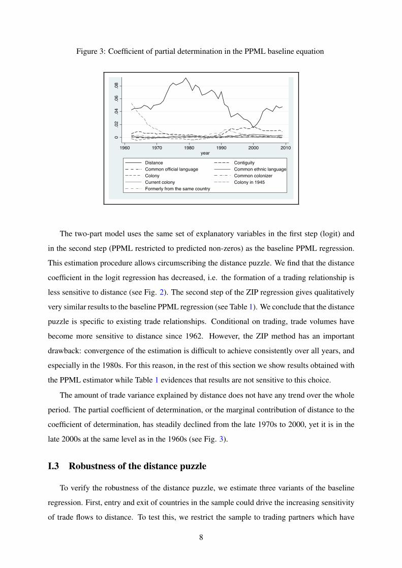
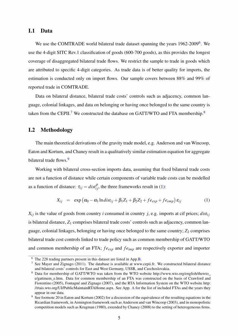
Figure 3: Coefficient of partial determination in the PPML baseline equation

0.0

2.0

4.0

6.0

8.1

1960 1970 1980 1990 2000 2010year

Distance Contiguity Common official language Common ethnic language Colony Common colonizer Current colony Colony in 1945 Formerly from the same country

The two-part model uses the same set of explanatory variables in the first step (logit) and

in the second step (PPML restricted to predicted non-zeros) as the baseline PPML regression.

This estimation procedure allows circumscribing the distance puzzle. We find that the distance

coefficient in the logit regression has decreased, i.e. the formation of a trading relationship is

less sensitive to distance (see Fig. 2). The second step of the ZIP regression gives qualitatively

very similar results to the baseline PPML regression (see Table 1). We conclude that the distance

puzzle is specific to existing trade relationships. Conditional on trading, trade volumes have

become more sensitive to distance since 1962. However, the ZIP method has an important

drawback: convergence of the estimation is difficult to achieve consistently over all years, and

especially in the 1980s. For this reason, in the rest of this section we show results obtained with

the PPML estimator while Table 1 evidences that results are not sensitive to this choice.

The amount of trade variance explained by distance does not have any trend over the whole

period. The partial coefficient of determination, or the marginal contribution of distance to the

coefficient of determination, has steadily declined from the late 1970s to 2000, yet it is in the

late 2000s at the same level as in the 1960s (see Fig. 3).

I.3 Robustness of the distance puzzle

To verify the robustness of the distance puzzle, we estimate three variants of the baseline

regression. First, entry and exit of countries in the sample could drive the increasing sensitivity

of trade flows to distance. To test this, we restrict the sample to trading partners which have

8

non-zero trade both ways in every year over 1962-2009. This leaves 786 stable two-way pairs.17

Fig. 4 shows that the sample effect does not reduce the distance puzzle.

Figure 4: Distance coefficient in sample of stable pairs (PPML)

.4.5

.6.7

.8

1960 1970 1980 1990 2000 2010year

Distance coefficient Confidence intervalConfidence interval Linear trendCovered share of world trade

Distance coefficient - Superbalanced PPML regression

Second, the changing composition of trade in terms of goods could explain the distance

puzzle. To compute the impact of the composition effect, trade shares of each good in total

trade are fixed at their 1962 values. As shown by Fig. 5, the composition effect deepens the

distance puzzle.18

Contrasting both Fig. 4 and Fig. 5 with Fig. 1, it is interesting to remark that most short-

term fluctuations of the distance coefficient seem to be explained by sample and composition

effects.

Third, we check whether controlling for countries’ selection into FTAs and GATT/WTO

membership reduces the distance puzzle. Separate controls are included for each FTA. 19

As shown in Fig. 6, controlling for countries’ participation into free trade agreements solves

the distance puzzle. However, this effect is mechanical. Fig. 7 shows that the share of intra-

FTA trade among nearby (less than 2000 km) countries has increased from 38% in 1962 to

17 This is a rectangular sample which includes 32 countries: Argentina, Belgium-Luxembourg, Brazil, Canada,Chile, Colombia, Denmark, France, Germany, Great Britain, Greece, Hong Kong, Iceland, Israel, Italy, Japan,Malaysia, Mexico, Netherlands, Philippines, Portugal, Paraguay, Singapor, South Korea, Spain, Sweden,Switzerland, Thailand, Tunisia, Turkey, Venezuela and the USA. China, India, Sub-Saharan African, Cen-tral and Eastern European countries do not have a reciprocal trading relationship in all years with any singlecountry, and are thus excluded.

18 Robustness checks have been conducted using 1984 and 2009 weights. Results are qualitatively similar.19 See Appendix A for the full list of included FTAs. Restricting this list to the "main" FTAs (EC and EU, USA-

Canada FTA and NAFTA, the Comecon,EFTA, ASEAN, Mercosur, as well as GATT-WTO) leads to the sameresult.

9

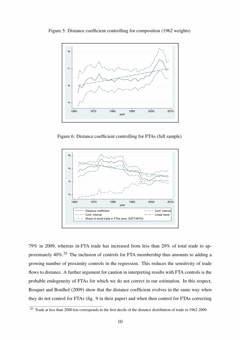
Figure 5: Distance coefficient controlling for composition (1962 weights)

.5.6

.7.8

1960 1970 1980 1990 2000 2010year

Distance coefficient controling for composition (1962 weight, PPML)

Figure 6: Distance coefficient controlling for FTAs (full sample)

.2.4

.6.8

1960 1970 1980 1990 2000 2010year

Distance coefficient Conf. intervalConf. interval Linear trendShare of world trade in FTAs (excl. GATT/WTO)

Distance coefficient - regressions including all FTA

79% in 2009, whereas in-FTA trade has increased from less than 20% of total trade to ap-

proximately 40%.20 The inclusion of controls for FTA membership thus amounts to adding a

growing number of proximity controls in the regression. This reduces the sensitivity of trade

flows to distance. A further argument for caution in interpreting results with FTA controls is the

probable endogeneity of FTAs for which we do not correct in our estimation. In this respect,

Bosquet and Boulhol (2009) show that the distance coefficient evolves in the same way when

they do not control for FTAs (fig. 9 in their paper) and when then control for FTAs correcting

20 Trade at less than 2000 km corresponds to the first decile of the distance distribution of trade in 1962-2009.

10

for endogeneity (fig. 11 in their paper).

Figure 7: Share of intra-FTA trade among nearby countries (2000km or less)

.2.4

.6.8

1

1960 1970 1980 1990 2000 2010year

Excluding contiguous countries All

Share of intra-FTA trade (2000 km or less)

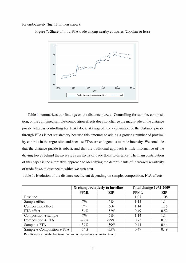
Table 1 summarizes our findings on the distance puzzle. Controlling for sample, composi-

tion, or the combined sample-composition effects does not change the magnitude of the distance

puzzle whereas controlling for FTAs does. As argued, the explanation of the distance puzzle

through FTAs is not satisfactory because this amounts to adding a growing number of proxim-

ity controls in the regression and because FTAs are endogenous to trade intensity. We conclude

that the distance puzzle is robust, and that the traditional approach is little informative of the

driving forces behind the increased sensitivity of trade flows to distance. The main contribution

of this paper is the alternative approach to identifying the determinants of increased sensitivity

of trade flows to distance to which we turn next.

Table 1: Evolution of the distance coefficient depending on sample, composition, FTA effects

% change relatively to baseline Total change 1962-2009PPML ZIP PPML ZIP

Baseline 1.07 1.08Sample effect 7% 5% 1.14 1.14Composition effect 7% 6% 1.14 1.15FTA effect -54% -52% 0.49 0.52Composition + sample 7% 5% 1.14 1.14Composition + FTA -29% -29% 0.75 0.77Sample + FTA -59% -59% 0.44 0.44Sample + Composition + FTA -54% -55% 0.49 0.49Results reported in the last two columns correspond to a geometric trend.

11

II Interpreting the distance coefficient

The distance coefficient, or the elasticity of trade to distance, is the product of two elastici-

ties: the elasticity of trade costs to distance and the elasticity of trade flows to trade costs. The

three main microfoundations of the gravity model of trade give structurally different interpreta-

tions to the elasticity of trade flows to distance.

II.1 The three main microfoundations

In Eaton and Kortum (2), consumers shop around the world for the cheapest supplier of each

sectoral good. Bilateral exports are a function of total sales of exporter i, of total expenditure of

importer j, as well as of the total world market as perceived by exporter i. Bilateral exports are

also a function of bilateral trade barriers of exporter i with importer j, and of the price index (p j)

of the importer. The parameter θ captures the degree of heterogeneity in productive efficiency

within countries across goods, i.e. the strength of comparative advantage. A higher value of

this parameter generates less heterogeneity in domestic producers’ efficiency across the set of

goods. Comparative advantage exerts a weaker force against trade resistance imposed by trade

barriers: the elasticity of trade to trade costs is higher in absolute value.21

Xi j =

(τi jp j

)−θ

YiYj

∑Nn=1

(τinpn

)−θ

Yn

(2)

In Chaney (3), consumers value the varieties of goods produced by heterogenous firms in a

monopolistic competition setting. Bilateral exports are a function of the share of expenditure

µ on goods which trade is costly,22 the nominal income of trading partners, world income,

fixed and variable bilateral trade costs ( fi j and τi j, respectively), workers’ productivity in the

exporting country wi, and a measure of importer’s remoteness θ j.23 The parameter γ is the shape

parameter of the Pareto distribution. It measures the degree of firm productivity heterogeneity

in the costly-trade sector. The elasticity of trade to variable trade costs no longer depends on

consumer preferences in the heterogeneous firms’ framework. Rather, it is firms’ efficiency

dispersion which determines the aggregate trade elasticity: the lower the degree of efficiency

21 See Eaton and Kortum (2002).22 The remaining expenditure is allocated to the numeraire sector producing a homogeneous freely tradable good.23 This remoteness measure is reminiscent of MR terms in Anderson and van Wincoop (2003), but it also accounts

for firm heterogeneity in productivity and fixed bilateral trade costs. See Chaney (2008).

12

dispersion in domestic markets, the higher the trade elasticity.24

The intuition for this result is given in Chaney (2008). The parameter γ is increasing in

the fraction of small size low-productivity firms. If firms’ efficiency dispersion is relatively

low, the efficiency cut-off above which firms are able to acquire export status is in proximity

of a substantial mass of firms. A reduction in trade barriers decreases the cut-off productivity

needed to acquire exporter status, and this triggers entry of relatively many firms into exporting:

lower efficiency dispersion among firms corresponds to an amplification of the aggregate trade

elasticity through the extensive margin.25 The degree of substitutability between firm-level

varieties is measured by σ f .

Xi j = µYiYj

Y

(wiτi j

θ j

)−γ

f−(

γ

σ f−1−1)

i j (3)

In Anderson and van Wincoop (4), there is no intersectoral or intrasectoral heterogeneity in

productive efficiency. The heterogeneity dimension comes from the assumption that goods pro-

duced by different countries are not homogeneous. Each country is specialized in production of

country-specific varieties which on aggregate give a country-specific composite good. Bilateral

exports Xi j are a function of the nominal income of each trading partner Yi, j, of world income Y ,

of bilateral trade costs τi j, and of multilateral trade resistance terms Πi, Pj.26 The parameter σ is

the ‘lower tier’ Armington elasticity of substitution which measures the degree of substitutabil-

ity of goods of different national origin (The ‘upper-tier’ elasticity pertains to substitutability

of domestic products and an aggregate import good while the ‘lower-tier’ elasticity measures

substitutability between importers of a given good: Sato (1967); Reinert and Shiells (Reinert

and Shiells); Saito (2004)).27

Xi j =

(YiYj

Y

)(τi j

ΠiPj

)−(σ−1)

(4)

To sum up, all theoretical frameworks used to derive the gravity equation are characterized

by a common feature: the elasticity of trade flows to trade costs, the ‘trade elasticity’, is de-

24 See the technical appendix to Chaney (2008) for the proof that the elasticity of trade flows to variable tradecosts is common across countries and equal to γ under the small country assumption.

25 Productivity is distributed over [1,+∞) as follows: P(

φ̃k < φ

)= Gk (φ) = 1− φ−γk where φ is unit labour

productivity. Firm-specific productivity determines the marginal cost of production (ci = wi/φ ) where thewage wi is pinned down by country-specific labor productivity in the numeraire sector .

26 Πi, Pj are respectively inward and outward MR terms.27 See Anderson and van Wincoop (2003). In monopolistic competition with homogenous firms the trade elasticity

parameter corresponds to the substitution elasticity between firm-level varieties (Dixit and Stiglitz (1977);Krugman (1980)). The structure of the equation would be similar, however.

13

creasing in the degree of heterogeneity observed in a single dimension, and it is this dimension

which is framework-specific.28 The coefficient of interest α1 from equation (1) has a different

structural interpretation in each framework:

αARMINGTON1 = ρ (σ −1); αRICARDO

1 = ρθ ; αHET−FIRMS1 = ργ .

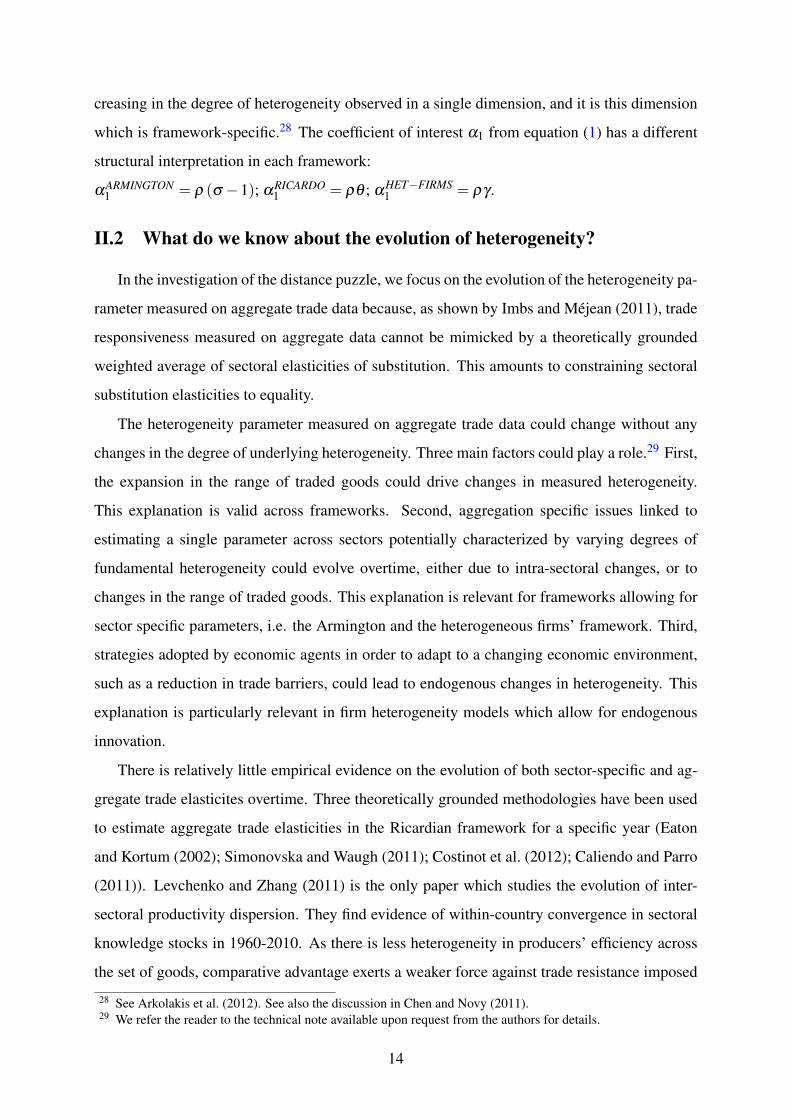
II.2 What do we know about the evolution of heterogeneity?

In the investigation of the distance puzzle, we focus on the evolution of the heterogeneity pa-

rameter measured on aggregate trade data because, as shown by Imbs and Méjean (2011), trade

responsiveness measured on aggregate data cannot be mimicked by a theoretically grounded

weighted average of sectoral elasticities of substitution. This amounts to constraining sectoral

substitution elasticities to equality.

The heterogeneity parameter measured on aggregate trade data could change without any

changes in the degree of underlying heterogeneity. Three main factors could play a role.29 First,

the expansion in the range of traded goods could drive changes in measured heterogeneity.

This explanation is valid across frameworks. Second, aggregation specific issues linked to

estimating a single parameter across sectors potentially characterized by varying degrees of

fundamental heterogeneity could evolve overtime, either due to intra-sectoral changes, or to

changes in the range of traded goods. This explanation is relevant for frameworks allowing for

sector specific parameters, i.e. the Armington and the heterogeneous firms’ framework. Third,

strategies adopted by economic agents in order to adapt to a changing economic environment,

such as a reduction in trade barriers, could lead to endogenous changes in heterogeneity. This

explanation is particularly relevant in firm heterogeneity models which allow for endogenous

innovation.

There is relatively little empirical evidence on the evolution of both sector-specific and ag-

gregate trade elasticites overtime. Three theoretically grounded methodologies have been used

to estimate aggregate trade elasticities in the Ricardian framework for a specific year (Eaton

and Kortum (2002); Simonovska and Waugh (2011); Costinot et al. (2012); Caliendo and Parro

(2011)). Levchenko and Zhang (2011) is the only paper which studies the evolution of inter-

sectoral productivity dispersion. They find evidence of within-country convergence in sectoral

knowledge stocks in 1960-2010. As there is less heterogeneity in producers’ efficiency across

the set of goods, comparative advantage exerts a weaker force against trade resistance imposed

28 See Arkolakis et al. (2012). See also the discussion in Chen and Novy (2011).29 We refer the reader to the technical note available upon request from the authors for details.

14

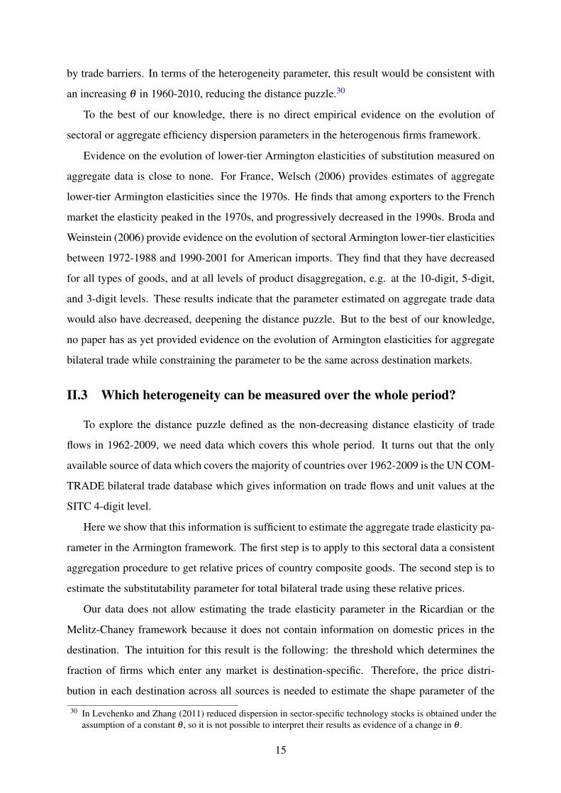
by trade barriers. In terms of the heterogeneity parameter, this result would be consistent with

an increasing θ in 1960-2010, reducing the distance puzzle.30

To the best of our knowledge, there is no direct empirical evidence on the evolution of

sectoral or aggregate efficiency dispersion parameters in the heterogenous firms framework.

Evidence on the evolution of lower-tier Armington elasticities of substitution measured on

aggregate data is close to none. For France, Welsch (2006) provides estimates of aggregate

lower-tier Armington elasticities since the 1970s. He finds that among exporters to the French

market the elasticity peaked in the 1970s, and progressively decreased in the 1990s. Broda and

Weinstein (2006) provide evidence on the evolution of sectoral Armington lower-tier elasticities

between 1972-1988 and 1990-2001 for American imports. They find that they have decreased

for all types of goods, and at all levels of product disaggregation, e.g. at the 10-digit, 5-digit,

and 3-digit levels. These results indicate that the parameter estimated on aggregate trade data

would also have decreased, deepening the distance puzzle. But to the best of our knowledge,

no paper has as yet provided evidence on the evolution of Armington elasticities for aggregate

bilateral trade while constraining the parameter to be the same across destination markets.

II.3 Which heterogeneity can be measured over the whole period?

To explore the distance puzzle defined as the non-decreasing distance elasticity of trade

flows in 1962-2009, we need data which covers this whole period. It turns out that the only

available source of data which covers the majority of countries over 1962-2009 is the UN COM-

TRADE bilateral trade database which gives information on trade flows and unit values at the

SITC 4-digit level.

Here we show that this information is sufficient to estimate the aggregate trade elasticity pa-

rameter in the Armington framework. The first step is to apply to this sectoral data a consistent

aggregation procedure to get relative prices of country composite goods. The second step is to

estimate the substitutability parameter for total bilateral trade using these relative prices.

Our data does not allow estimating the trade elasticity parameter in the Ricardian or the

Melitz-Chaney framework because it does not contain information on domestic prices in the

destination. The intuition for this result is the following: the threshold which determines the

fraction of firms which enter any market is destination-specific. Therefore, the price distri-

bution in each destination across all sources is needed to estimate the shape parameter of the

30 In Levchenko and Zhang (2011) reduced dispersion in sector-specific technology stocks is obtained under theassumption of a constant θ , so it is not possible to interpret their results as evidence of a change in θ .

15

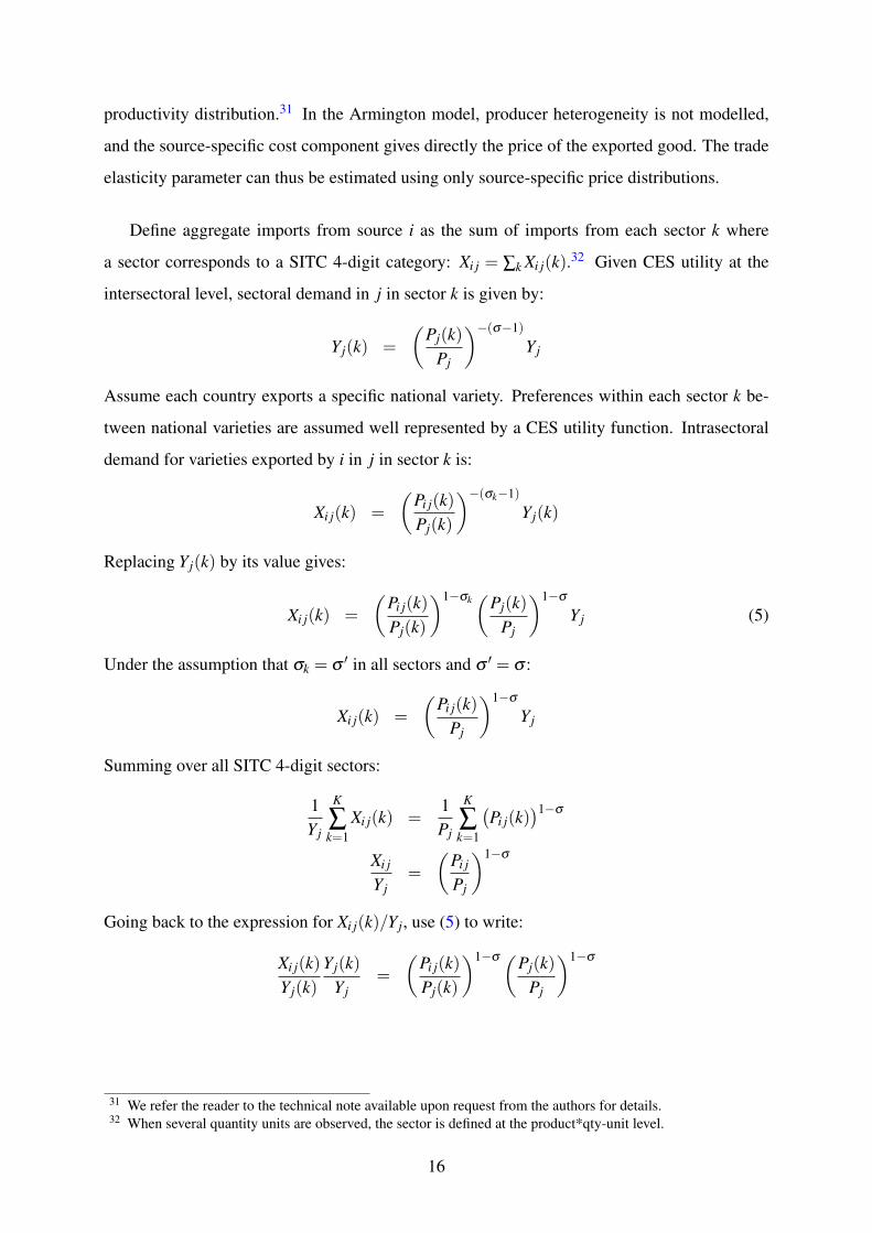
productivity distribution.31 In the Armington model, producer heterogeneity is not modelled,

and the source-specific cost component gives directly the price of the exported good. The trade

elasticity parameter can thus be estimated using only source-specific price distributions.

Define aggregate imports from source i as the sum of imports from each sector k where

a sector corresponds to a SITC 4-digit category: Xi j = ∑k Xi j(k).32 Given CES utility at the

intersectoral level, sectoral demand in j in sector k is given by:

Yj(k) =

(Pj(k)

Pj

)−(σ−1)

Yj

Assume each country exports a specific national variety. Preferences within each sector k be-

tween national varieties are assumed well represented by a CES utility function. Intrasectoral

demand for varieties exported by i in j in sector k is:

Xi j(k) =

(Pi j(k)Pj(k)

)−(σk−1)

Yj(k)

Replacing Yj(k) by its value gives:

Xi j(k) =

(Pi j(k)Pj(k)

)1−σk(

Pj(k)Pj

)1−σ

Yj (5)

Under the assumption that σk = σ ′ in all sectors and σ ′ = σ :

Xi j(k) =

(Pi j(k)

Pj

)1−σ

Yj

Summing over all SITC 4-digit sectors:

1Yj

K

∑k=1

Xi j(k) =1Pj

K

∑k=1

(Pi j(k)

)1−σ

Xi j

Yj=

(Pi j

Pj

)1−σ

Going back to the expression for Xi j(k)/Yj, use (5) to write:

Xi j(k)Y j(k)

Yj(k)Yj

=

(Pi j(k)Pj(k)

)1−σ (Pj(k)Pj

)1−σ

31 We refer the reader to the technical note available upon request from the authors for details.32 When several quantity units are observed, the sector is defined at the product*qty-unit level.

16

Replacing Pj(k)Pj

by its value and defining Y j(k)Y j

= ω j(k), we get:

Xi j(k)Yj(k)

Y j(k)Y j

=

[Pi j(k)Pj(k)

(ω j(k)

)1/1−σ

]1−σ

Summing over all SITC 4-digit sectors:

K

∑k=1

Xi j(k)Yj(k)

Yj(k)Yj

=K

∑k=1

ω j(k)[

Pi j(k)Pj(k)

]1−σ

Multiplying and dividing the right hand side of the expression by ω j(k)1−σ and taking logs:

ln[

Xi j

Y j

]= ln

{K

∑k=1

ω j(k)σ

[ω j(k)

Pi j(k)Pj(k)

]1−σ}

(6)

Working with the right hand side of (6), and using the approximation that for a large number of

sectors k, ln∑k Xk,i j ≈ ∑k lnXk,i j:

ln

{K

∑k=1

ω j(k)σ

[ω j(k)

Pi j(k)Pj(k)

]1−σ}≈

K

∑k=1

ln[ω j(k)σ

]+

K

∑k=1

ln

[(ω j(k)

Pi j(k)Pj(k)

)1−σ]

The first term disappears because:

σ ∑k

lnωk, j ≈ σ ln

(∑k

Yk, j/Y j

)= ζ ln1 = 0

Using the same approximation as previously for the second term:

(1−σ)K

∑k=1

ln[

ω j(k)Pi j(k)Pj(k)

]≈ (1−σ) ln

[K

∑k=1

ω j(k)Pi j(k)Pj(k)

]

The market share equation for aggregate bilateral trade as a function of the weighted average of

sectoral relative prices of i in j is:

ln[

Xi j

Yj

]≈ −(σ −1) ln

[K

∑k=1

ω j(k)Pi j(k)Pj(k)

](7)

Exponentiating gives the equation to be estimated:

Xi j/Yj = exp

[λ0− (σ −1) ln

(∑k

ωkPi j(k)Pj(k)

)+ f eexp + f eimp

]ηi j (8)

where f eexp and f eimp are source and destination fixed effects, ηi j is a multiplicative error term,

and λ0 is a constant. Source fixed effects control for the world preference for products of this

origin. Destination fixed effects control for unobserved domestic prices. The PPML estimator

17

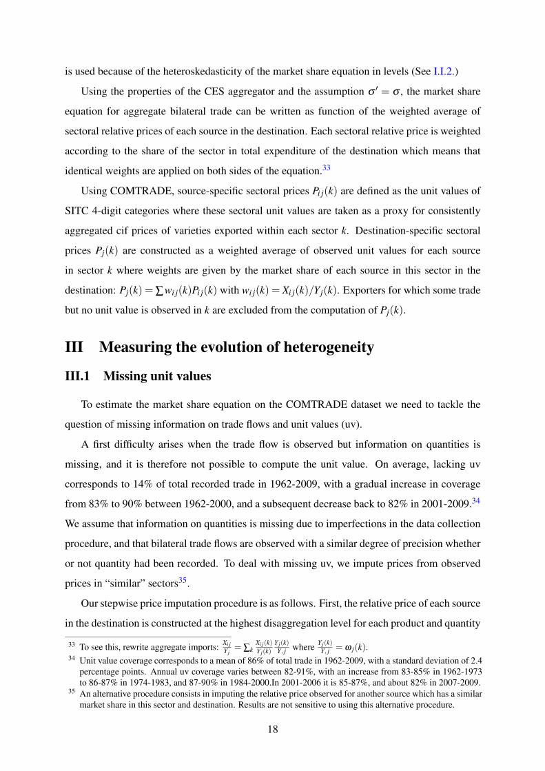
is used because of the heteroskedasticity of the market share equation in levels (See I.I.2.)

Using the properties of the CES aggregator and the assumption σ ′ = σ , the market share

equation for aggregate bilateral trade can be written as function of the weighted average of

sectoral relative prices of each source in the destination. Each sectoral relative price is weighted

according to the share of the sector in total expenditure of the destination which means that

identical weights are applied on both sides of the equation.33

Using COMTRADE, source-specific sectoral prices Pi j(k) are defined as the unit values of

SITC 4-digit categories where these sectoral unit values are taken as a proxy for consistently

aggregated cif prices of varieties exported within each sector k. Destination-specific sectoral

prices Pj(k) are constructed as a weighted average of observed unit values for each source

in sector k where weights are given by the market share of each source in this sector in the

destination: Pj(k) = ∑wi j(k)Pi j(k) with wi j(k) = Xi j(k)/Yj(k). Exporters for which some trade

but no unit value is observed in k are excluded from the computation of Pj(k).

III Measuring the evolution of heterogeneity

III.1 Missing unit values

To estimate the market share equation on the COMTRADE dataset we need to tackle the

question of missing information on trade flows and unit values (uv).

A first difficulty arises when the trade flow is observed but information on quantities is

missing, and it is therefore not possible to compute the unit value. On average, lacking uv

corresponds to 14% of total recorded trade in 1962-2009, with a gradual increase in coverage

from 83% to 90% between 1962-2000, and a subsequent decrease back to 82% in 2001-2009.34

We assume that information on quantities is missing due to imperfections in the data collection

procedure, and that bilateral trade flows are observed with a similar degree of precision whether

or not quantity had been recorded. To deal with missing uv, we impute prices from observed

prices in “similar” sectors35.

Our stepwise price imputation procedure is as follows. First, the relative price of each source

in the destination is constructed at the highest disaggregation level for each product and quantity

33 To see this, rewrite aggregate imports: Xi jY j

= ∑kXi j(k)Y j(k)

Y j(k)Y, j where Y j(k)

Y, j = ω j(k).34 Unit value coverage corresponds to a mean of 86% of total trade in 1962-2009, with a standard deviation of 2.4

percentage points. Annual uv coverage varies between 82-91%, with an increase from 83-85% in 1962-1973to 86-87% in 1974-1983, and 87-90% in 1984-2000.In 2001-2006 it is 85-87%, and about 82% in 2007-2009.

35 An alternative procedure consists in imputing the relative price observed for another source which has a similarmarket share in this sector and destination. Results are not sensitive to using this alternative procedure.

18

unit in which the source is active (which we call “4’-digit level”). Second, we proceed level by

level for aggregation: the relative price of the composite sectoral good of the source is first

constructed at the 4-digit level using the weighted average relative price observed at the 4’-digit

level, with destination-specific weights for each variety of the 4’-digit good the source is active

in. Given relative prices constructed at the 4-digit level, destination-specific weights are used to

aggregate these up to the 3-digit level, and so on until the relative price for the composite good

is constructed using relative prices at the 1-digit level. This improves the estimation of prices, if

one assumes that missing destination-specific relative prices at the 4’-digit can be approximated

by the mean observed destination-specific relative price among the corresponding 4-digit group

(and similarly at each aggregation level).

III.2 Zero trade flows

A second difficulty arises when both quantity and trade data are missing. Zero trade flows

(ztf) are a prevalent feature of the data while under model assumptions some trade should be

observed in every sector k between all pairs i j.36

We assume that this information is missing because the underlying trade flow is positive

but so small that it does not pass the threshold applied by the data collecting authorities (in

UN COMTRADE this threshold corresponds to 1000 USD). Such flows, if recorded, would not

substantially modify the distribution of observed market shares in the destination (the left hand

side of (8)), because they are an order of magnitude smaller than observed trade.

We use the same stepwise price imputation as in the case of missing unit values. This is

problematic because the constructed relative price of the composite good systematically under-

estimates the true underlying relative price. Under model assumptions, statistically unobserved

trade values must correspond to a higher cif price than the maximum observed price in the desti-

nation across all sources and sectors while by construction we postulate that unobserved relative

prices in ztf sectors are equal to a weighted average relative price across sectors in which trade

is observed.

The assumption we make on unobserved prices would not be problematic if the underesti-

mation factor were constant across exporters.37 This scalar would cancel out across sources,

36 The share of observed SITC 4-digit flows relatively to the total number of potential SITC 4-digit bilateral tradeflows increases from 10% to 14% in 1962-2009.

37 An alternative method consists in imputing unobserved relative prices with some arbitrary price above themaximum observed in the destination. As ztf constitute 85-90% of all 4-digit trade flows, this method isproblematic because results are driven by imputed rather than effectively observed prices.

19

and the estimated substitutability parameter would correspond to the true parameter. This is

obviously not the case. Table 2 shows that the underestimation factor is not constant across

exporters: the share of ztf is strongly decreasing in market share. The relative price of the com-

posite good is underestimated by more for small exporters. For a given observed distribution

of market shares, the underlying dispersion in relative prices of the composite good is greater

than the observed dispersion in relative prices. The estimated parameter σ̃ overestimates the

true substitutability parameter σ .

Table 2 shows that the reduction in the share of ztf proceeds at quicker pace in 1962-2009

for small exporters: the coefficient for the interaction term for the market share and year is

significant and positive. Table 3 presents the predicted share of ztf for four types of exporters

in 1962 and 2009. For a very small exporter with .02% market share, the initial share of ztf

is predicted to be .95, and it is reduced to .83 by 2009, i.e. a 12 percentage point decrease.

Consider a relatively big exporter, with a 10% market share: its share of ztf is reduced from

.72 to .65, a 7 percentage point decrease. As the gap between the share of ztf for big and small

exporters is reduced overtime, the overestimation bias of σ̃ is progressively reduced.

Table 2: Proportion of zero trade flows as a function of market share

depvar:Share of ZTF

(1) (2) (3) (4)

ms -0.0401*** -0.2446*** -0.0427*** -0.2573***(0.0001) (0.0134) (0.0001) (0.013)

year -0.0029*** -0.0020*** -0.0033*** -0.0024***(0.0000) (0.0001) (0.0000) (0.000)

ms∗ year 0.0001*** 0.0001***(0.0000) (0.000)

constant 5.3474*** 3.5852*** 6.0976*** 4.2515***(0.0335) (0.1372) (0.0366) (0.134)

Destination FE NO NO YES YESObservations 657001 657001 657001 657001

Notes: The share of ZTF is computed at the SITC 4-digit level. The estimation is conducted in PPMLin order to include observations where ztf=0. The log of the market share is used in the estimation.Destination fixed effects are included in (3) and (4). Robust standard errors are in parentheses. *** p<0.01.

20

Table 3: Predicted share of ztf for exporters with different market share, 4-digit level

year ms=0.02% ms=1% ms=10% ms=28.7%

1962 0.95 0.80 0.72 0.69

2009 0.83 0.71 0.65 0.62

Columns (1) and (4) correspond to the mean and to 2 st. deviations above the mean in the distribution of log market share.Columns (2) and (3) correspond to the mean and to 2 st. deviations above the mean in the distribution of market share.

Thus, the hypothesis we make on unobserved sectoral prices in ztf sectors does not always

impede interpreting the evolution of the underlying substitutability parameter. In particular, if

it is found that the estimated parameter increases in absolute value, this evolution necessarily

provides a lower bound on the increase in the underlying substitutability parameter. This is

because the overestimation bias is reduced overtime.

Figure 8 presents the results on the evolution of σ̃ obtained when (8) is estimated on annual

crossections of the COMTRADE dataset. The absolute value of trade elasticity has increased

by about 29% from 1962 to 2009.

−.8

−.6

−.4

−.2

1960 1970 1980 1990 2000 2010year

coef_elast linear fit

Trade elasticity (0−digit level)

Figure 8: Estimated (1− σ̃)

21

III.3 Robustness checks

III.3.1 Changing the dataset

We provide a robustness check by estimating the evolution of the heterogeneity parameter

for aggregate bilateral trade on a different dataset. We use the BACI dataset which reports bilat-

eral trade data at the HS-1992 6-digit disaggregation level for 1995-2009. The accuracy of the

relative prices of country-composite goods constructed with this dataset is improved because the

harmonization procedure applied by Gaulier and Zignago (2010) in constructing BACI yields

much better-quality unit values while substantially reducing the number of observations with

lacking unit value. As a result, at the 6-digit level, less than 7% of total reported trade in BACI

has missing unit values. This is reduced to 1-3% of total trade when the data is aggregated to

the 4-digit level, as opposed to more than 10% in the raw COMTRADE data we originally used.

Another advantage is that the share of ztf in BACI is stable in 1995-2009 as opposed to rela-

tively strong fluctuations in the share of ztf overtime in our original dataset. The disadvantage

of BACI is that it covers only a relatively short period compared to the years over which the dis-

tance puzzle exists. Obviously, we do not expect to reproduce exactly the results obtained with

our original dataset because the trade classification and its level of aggregation are different.

−.4

−.3

−.2

−.1

0

.1

1995 2000 2005 2010

year

Elasticity(baci) confidence interval

Aggregate elasticity (baci database)

Figure 9: Estimated (1− σ̃), BACI database

Fig. 9 shows that our results hold: the elasticity parameter is found to increase in absolute

value from 1995-2009. This can be compared with the equivalent period in our original dataset:

the increase in the elasticity is much steeper on the BACI dataset. This finding supports the

idea that our benchmark estimation results likely provide a lower bound on the increase in the

22

aggregate trade elasticity. However, the level of the elasticity estimated in 1995-1999 on BACI

data is puzzling and suggests the existence of an attenuation bias. This is the focus of our second

robustness check.

III.3.2 Instrumenting: motivation and results

The results just presented are subject to caution if supply schedules are not horizontal.38

In that case, the demand elasticity parameter estimated in the market share equation will suffer

from attenuation bias due to not controlling for potentially positive and finite supply elasticities.

This attenuation bias would not be problematic for analyzing the evolution of the substitutability

parameter if only the level of the parameter were affected. The problem arises because, as shown

by Feenstra (1994), the attenuation bias also impacts the evolution of the parameter.

Feenstra has developed an instrumental variables’ approach which solves this problem (see

Feenstra (1994), and refinements in Broda and Weinstein (2006) and Imbs and Méjean (2011)).

This method exploits year-to-year variations in relative prices and market shares over 10- to 20-

year estimation windows to compute the Armington elasticity. We refrain from this approach

for two sets of reasons. First, Feenstra’s method relies on the assumption that the elasticity

parameter remains constant through time, whereas we want to allow the parameter to vary

in each year. Second, more fundamentally, Feenstra’s elasticity parameter determines short-

run, marginal, longitudinal effects whereas we are interested in the elasticity parameter which

determines long-run, equilibrium, cross-section outcomes. It is not immediate that these two

elasticities should be the same.

In this paper, we opt for a different approach in order to preserve the time dimension which

is central to our analysis. We would like to have an an instrument which adequately captures

exporter-specific shocks to the price of the composite good which are not demand-driven, such

as exogenous shocks to inputs’ prices. One possibility would be the Producer Price Index (PPI)

since it captures the evolution of prices faced by producers on the inputs’ side. Unfortunately,

we do not have PPI data for most countries and years in our sample. We therefore settle for an

alternative exporter-specific price level indicator: the GDP price level in current US dollars as

reported in the Penn World Tables for 189 countries in 1950-2009.39

38 Broda et al. (2006) find evidence of non-horizontal supply schedules at the 4-digit disaggregation level. Mageeand Magee (2008) provide evidence that the small country assumption may in fact hold in the data in whichcase there would be no attenuation bias.

39 See Heston et al. (2011). Our sample of countries does not coincide perfectly with the countries in the PennWorld Tables. However, as it is the smallest exporters which drop out, the sample adjustment in terms of worldtrade coverage is minor.

23

The instrumenting procedure is the following. First, we compute relative prices for exporter-

specific composite goods in each destination market using the stepwise price imputation proce-

dure (see III.1). Second, for each destination market, we compute the mean evolution of GDP

price levels in current US dollars of its trading partners, weighted by their market shares in

this destination. This amounts to computing the evolution of the relevant real exchange rate for

each specific bilateral trade relation. Third, we compute a hypothetical relative price at time

t for each exporter in each market as the product of its relative price at time (t − 1) and the

evolution of its GDP price level between t and (t − 1) relatively to all other trading partners

in this destination. Fourth, we predict the relative price of each exporter in each destination at

time t by regressing its observed relative price on this hypothetical relative price. This gives an

instrumented relative price for each exporter which depends only on its past relative price and

the relative evolution of its GDP price level. Finally, we estimate (8) using these instrumented

relative prices instead of the observed relative prices.

It could be argued that allowing for just one lag inadequately captures the temporal rela-

tionship between shocks to inputs’ prices and their pass-through to the price of exported output.

Indeed, if prices are relatively persistent, the instrumenting procedure would amount to little

more than replacing observed prices in t with lagged observed prices in (t− 1). We therefore

also estimate (8) using as instrument the evolution of each exporter’s GDP price level relatively

to all other trading partners in the destination between (t− s) and t where s = 1, ...,10.

Results obtained with one lag (s = 1) are shown in Fig.10. The absolute value of the sub-

stitutability parameter has increased by 13% in 1962-2009 while its level increases by 9% on

average relatively to the estimate obtained with non-instrumented prices.

This result is robust to increasing the number of periods in which the evolution of exports’

prices is predicted with the evolution of domestic prices (see Appendix C). Thus, for s = 10, the

elasticity increases by 29% in 1972-2009 (compared to 26% for s = 1 over the same period).

The evolution of the parameter becomes steeper as we increase the number of lags. Therefore,

it is likely that our estimate provides a lower bound on the increase in the true substitutability

parameter.

III.4 Is there a distance puzzle left?

This section has provided empirical evidence on the evolution of the aggregate substitutabil-

ity parameter for world trade in 1962-2009. This substitutability parameter corresponds to the

24

−1

−.8

−.6

−.4

−.2

1960 1970 1980 1990 2000 2010year

Trade elasticity (instrumented relative price, 1 lag)

Figure 10: Estimated (1− σ̃), instrumented relative price of composite good, 1 lag

aggregate trade elasticity in the Armington framework. We find that this parameter has in-

creased by 29% between 1962 and 2009 in the benchmark estimation, and by 13% when relative

prices are instrumented. Both estimates are likely to be providing lower bounds on the increase

in the true substitutability parameter. Section I has shown that the distance elasticity of trade has

increased by 8% over the same period. Combining these two results to evaluate the magnitude

of the distance puzzle redefined as increasing elasticity of trade costs to distance, we conclude

that there is no distance puzzle in the framework of the Armington model in as much as the

elasticity of trade costs to distance has decreased by 4% in 1962-2009. The increasing distance

elasticity of trade is fully explained by increased perceived substitutability of country-specific

composite goods.

What is the economic interpretation of an increasing substitutability parameter measured on

aggregate data?

First, the degree of perceived similarity of country-composite goods may have increased.

Since the 1960s, a growing number of countries started producing a set of goods similar to

that of developed countries. This process has increased the number of available varieties and,

potentially, their degree of similarity.40

Second, composition effects may have lead to changes in the parameter estimated on ag-

gregate data. If the reduction in trade barriers has led to the expansion in the range of traded

goods, trade in previously non-traded sectors could modify measured substitutability of country-

40 Schott (2004) documents increased similarity in the set of exported goods of US trade partners while Brodaet al. (2006) document the increase in the number of imported varieties since the 1970s.

25

composite goods. Non-uniform reductions in sectoral trade costs would also modify the com-

position of world trade, leading to a change in the substitutability parameter measured on ag-

gregate data.

Ideally, we would like to separate out the impact of composition and sector-specific effects

to quantify the net effect of increased perceived similarity of country-composite goods. This is

however impossible because, as shown by Imbs and Méjean (2011), the parameter estimated on

aggregate data cannot be mimicked by a weighted average of sectoral parameters. The bottom

line is that an increase in measured substitutability for country-composite goods is consistent

with complex competition dynamics in price and quality documented by Amiti and Khandelwal

(2012) as well as with increased vertical specialization of countries within sectors documented

by Fontagné et al. (2008).

Conclusion

The estimated effect of distance in gravity equations has slightly increased in the past 50

years despite substantial innovation in transportation and communication: this is the ‘distance

puzzle’. Using COMTRADE 4-digit bilateral trade data in 1962-2009, this paper finds that

the evolution of the elasticity of trade flows to trade costs, referred to as the ‘trade elasticity’,

provides a direct explanation of the increasing distance elasticity of trade. Increased sensitivity

of trade flows to relative prices has more than compensated the reduction in the elasticity of

trade costs to distance.

The paper proceeds in three steps. First, it shows that the distance puzzle is a feature of

our data by estimating yearly cross-section gravity equations. In our baseline estimation the

distance coefficient has increased by 8% from 1962 to 2009. This result qualitatively holds

when we correct for changes in the sample of trading partners and the composition of world

trade. Taking into account FTAs seems to solve the distance puzzle, but this is an artefact

of their growing importance: introducing FTAs dummies amounts to adding a time-growing

number of proximity controls in the estimation.

Second, the paper underlines that in the main theoretical foundations of the gravity equation

the distance coefficient is the product of the elasticity of trade costs to distance and a measure

of heterogeneity. In the Ricardian framework, heterogeneity is intra-country and inter-sector.

The trade elasticity corresponds to the degree of dispersion in productivity within countries

across goods. In monopolistic competition with firm heterogeneity, the dispersion parameter

26

is intra-country and intra-sector. The trade elasticity corresponds to the degree of dispersion

in intrasectoral firm productivity. In the Armington framework, heterogeneity is inter-country

and intra-sector. The trade elasticity corresponds to the degree of perceived substitutability of

country-specific varieties of each good.

Third, the paper estimates the evolution of the trade elasticity in the Armington framework,

i.e. the substitution elasticity between country composite goods. It uses 4-digit unit values

as proxies for sectoral prices. In our method, unobserved unit values lead to an overestima-

tion bias that is reduced over time. As the estimated elasticity still increases in absolute value

this evolution provides a lower bound on the increase in the absolute value of the underlying

trade elasticity. Once instrumented, the estimated elasticity increases by 13% between 1962

and 2009. The evolution of the distance coefficient is thus compatible with a decrease of the

elasticity of trade costs to distance of at least 4%.

References

Amiti, M. and A. Khandelwal (2012). Import competition and quality upgrading. Review of

Economics and Statistics (forthcoming).

Anderson, J. E. and E. van Wincoop (2003). Gravity with gravitas: A solution to the border

puzzle. American Economic Review 93(1), 170–192.

Arkolakis, C., A. Costinot, and A. Rodriguez-Clare (2012). New trade models, same old gains?

American Economic Review 102(1), 94–130.

Armington, P. S. (1969). A theory of demand for products distinguished by place of production.

IMF Staff Papers 16(1), 159–178.

Baldwin, R. and J. Harrigan (2007). Zeros, quality and space: trade theory and trade evidence.

NBER Working Paper Series 13214.

Berthelon, M. and C. Freund (2008). On the conservation of distance in international trade.

Journal of International Economics 75(2), 310–320.

Bosquet, C. and H. Boulhol (2009). Gravity, log of gravity and the distance puzzle. GREQAM

Working Paper 2009(12).

27

Broda, C., J. Greenfield, and D. Weinstein (2006). From groundnuts to globalization: A struc-

tural estimate of trade and growth. NBER Working Paper Series 12512.

Broda, C., N. Limão, and D. Weinstein (2006). Optimal tariffs: The evidence. NBER Working

Paper Series 12033.

Broda, C. and D. E. Weinstein (2006). Globalization and the gains from variety. Quarterly

Journal of Economics 121(2), 541–585.

Brun, J.-F., C. Carrère, P. Guillaumont, and J. d. Melo (2005). Has distance died? evidence

from a panel gravity model. World Bank Economic Review 19, 99–120.

Buch, C. M., J. Kleinert, and F. Toubal (2004). The distance puzzle: on the interpretation of the

distance coefficient in gravity equations. Economics Letters 83, 293–298.

Burger, M. J., F. G. van Oort, and G.-J. Linders (2009). On the specification of the gravity model

of trade: Zeros, excess zeros and zero-inflated estimation. Spatial Economic Analysis 4(2),

167–190.

Cairncross, F. (1997). The Death of Distance: How the Communications Revolution will change

our Lives. London: Orion Business Books.

Caliendo, L. and F. Parro (2011). Estimates of the trade and welfare effects of nafta. mimeo,

University of Chicago.

Chaney, T. (2008). Distorted gravity: The intensive and extensive margins of international trade.

American Economic Review 98(4), 1707–1721.

Chen, N. and D. Novy (2011). Gravity, trade integration, and heterogeneity across industries.

Journal of International Economics 85(2), 206–221.

Coe, D., A. Subramanian, and N. Tamirisa (2007). The missing globalization puzzle: Evidence

of the declining importance of distance. IMF Staff Papers 54(1), 34–58.

Combes, P.-P., T. Mayer, and J.-F. Thisse (2006). Economie Géographique. Paris: Economica.

Costinot, A., D. Donaldson, and I. Komunjer (2012). What goods do countries trade? A quan-

titative exploration of Ricardo’s ideas. Review of Economics and Statistics (forthcoming).

28

Crawford, J.-A. and R. V. Fiorentino (2005). The changing landscape of regional trade agree-

ments. WTO Discussion Papers (8).

Daudin, G. (2003). La logistique de la mondialisation. Revue de l’OFCE (87), 411–435.

Daudin, G. (2005). Les transactions de la mondialisation. Revue de l’OFCE (92), 223–262.

Disdier, A.-C. and K. Head (2008). The puzzling persistence of the distance effect in bilateral

trade. The Review of Economics and Statistics 90(1), 37–48.

Dixit, A. K. and J. E. Stiglitz (1977). Monopolistic competition and optimum product diversity.

American Economic Review 67, 297–308.

Duranton, G. and M. Storper (2008). Rising trade costs. agglomeration and trade with endoge-

nous transaction costs. Canadian Journal of Economics 41(1), 292–319.

Eaton, J. and S. Kortum (2002). Technology, geography, and trade. Econometrica 70(5), 1741–

1779.

Feenstra, R. (1994). New product varieties and the measurement of international prices. The

American Economic Review 84(1), 157–177.

Feyrer, J. (2009). Trade and income: Exploiting time series in geography. NBER Working Paper

Series 14910.

Fontagné, L., G. Gaulier, and S. Zignago (2008). North-south competition in quality. Economic

Policy 23(53), 51–91.

Fontagné, L. and S. Zignago (2007). A re-evaluation of the impact of regional trade agreements

on trade patterns. Economic Internationale 109, 31–51.

Friedman, T. L. (2007). The World is Flat: A Brief History of the Twenty-first Century, 2nd

edition. Farrar Straus & Giroux.

Gaulier, G. and S. Zignago (2010). Baci: International trade database at the product level.

CEPII working papers (23).

Greene, W. (1994). Accounting for excess zeros and sample selection in poisson and negative

binomial regression models. Stern School of Business Department of Economics Working

Paper (94-10).

29

Greene, W. (2003). Econometric Analysis (5th ed.). Upper Saddle River, N.J.: Prentice Hall.

Helpman, E., M. Melitz, and Y. Rubinstein (2008). Estimating trade flows: trading partners and

trading volumes. Quarterly Journal of Economics 123(2), 441–487.

Heston, A., R. Summers, and B. Aten (2011, May). Penn world table version 7.0. Center for

International Comparisons of Production, Income and Prices at the University of Pennsylva-

nia.

Hummels, D. (1999). Have international transportation costs declined? Unpublished

manuscript, Purdue University.

Hummels, D. (2001). Towards a geography of trade costs. Unpublished manuscript, Purdue

University.

Hummels, D. (2007). Transportation costs and international trade in the second era of global-

ization. Journal of Economic Perspectives 21(3), 131–154.

Hummels, D. and G. Schaur (2012). Time as a trade barrier. NBER Working Paper Series 17758.

Imbs, J. and I. Méjean (2011). Elasticity optimism. CEPR Discussion Paper 7177.

Krugman, P. (1980). Scale economies, product differentiation, and the pattern of trade. Ameri-

can Economic Review 70, 950–959.

Lambert, D. (1992). Zero-inflated poisson regression, with an application to defects in manu-

facturing. Technometrics 34(1), 1–14.

Levchenko, A. A. and J. Zhang (2011). The evolution of comparative advantage: Measurement

and welfare implications. NBER Working Paper Series 16806.

Levinson, M. (2006). The Box: How the Shipping Container Made the World Smaller and the

World Economy Bigger. Princeton: Princeton University Press.

Magee, C. S. and S. P. Magee (2008). The united states is a small country in world trade. Review

of International Economics 16(5), 990–1004.

Manning, W. G. and J. Mullahy (1999). Estimating log models: To transform or not to trans-

form? NBER Technical Working Paper Series 246.

30

Márquez-Ramos, L., I. Martinez-Zarzoso, and C. Suárez-Burguet (2007). The role of distance in

gravity regressions: Is there really a missing globalization puzzle? B.E. Journal of Economic

Analysis and Policy 7(1).

Martin, W. and C. S. Pham (2008). Estimating the gravity model when zero trade flows are

frequent. World Bank Working Paper, unpublished.

Mayer, T. and S. Zignago (2011). Notes on CEPII’s distances measures: the GeoDist database.

MPRA Working Paper Series 36347.

Mullahy, J. (1986). Specification and testing of some modified count data models. Journal of

Econometrics 33(3), 341–365.

Reinert, K. A. and C. R. Shiells. Trade substitution elasticities for analysis of a north american

free trade area. Staff Research Study, USITC (19).

Saito, M. (2004). Armington elasticities in intermediate inputs’ trade: a problem in using

multilateral data. The Canadian Journal of Economics 37(4), 1097–1117.

Santos Silva, J. M. C. and S. Tenreyro (2006). The log of gravity. The Review of Economics

and Statistics 88(4), 641–658.

Sato, K. (1967). A two-level constant-elasticity-of-substitution production function. Review of

Economic Studies 34, 201–218.

Schott, P. (2004). Across product vs. within-product specialization in international trade. The

Quarterly Journal of Economics 119(2), 647–678.

Simonovska, I. and M. Waugh (2011). The elasticity of trade: Estimates and evidence. UC

Davis Working Paper 11.

Welsch, H. (2006). Armington elasticities and induced intra-industry specialization: The case

of france, 1970-1997. Economic Modelling 23, 556–567. Armington elasticities’ estimates

for France ’70-’90s.

31

A List of included FTAs

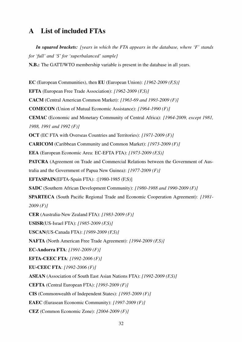
In squared brackets: [years in which the FTA appears in the database, where ‘F’ stands

for ‘full’ and ‘S’ for ‘superbalanced’ sample]

N.B.: The GATT/WTO membership variable is present in the database in all years.

EC (European Communities), then EU (European Union): [1962-2009 (F,S)]

EFTA (European Free Trade Association): [1962-2009 (F,S)]

CACM (Central American Common Market): [1963-69 and 1993-2009 (F)]

COMECON (Union of Mutual Economic Assistance): [1964-1990 (F)]

CEMAC (Economic and Monetary Community of Central Africa): [1964-2009, except 1981,

1988, 1991 and 1992 (F)]

OCT (EC FTA with Overseas Countries and Territories): [1971-2009 (F)]

CARICOM (Caribbean Community and Common Market): [1973-2009 (F)]

EEA (European Economic Area: EC-EFTA FTA): [1973-2009 (F,S)]

PATCRA (Agreement on Trade and Commercial Relations between the Government of Aus-

tralia and the Government of Papua New Guinea): [1977-2009 (F)]

EFTASPAIN(EFTA-Spain FTA): :[1980-1985 (F,S)]

SADC (Southern African Development Community): [1980-1988 and 1990-2009 (F)]

SPARTECA (South Pacific Regional Trade and Economic Cooperation Agreement): [1981-

2009 (F)]

CER (Australia-New Zealand FTA): [1983-2009 (F)]

USISR(US-Israel FTA): [1985-2009 (F,S)]

USCAN(US-Canada FTA): [1989-2009 (F,S)]

NAFTA (North American Free Trade Agreement): [1994-2009 (F,S)]

EC-Andorra FTA: [1991-2009 (F)]

EFTA-CEEC FTA: [1992-2006 (F)]

EU-CEEC FTA: [1992-2006 (F)]

ASEAN (Association of South East Asian Nations FTA): [1992-2009 (F,S)]

CEFTA (Central European FTA): [1993-2009 (F)]

CIS (Commonwealth of Independent States): [1995-2009 (F)]

EAEC (Eurasean Economic Community): [1997-2009 (F)]

CEZ (Common Economic Zone): [2004-2009 (F)]

32

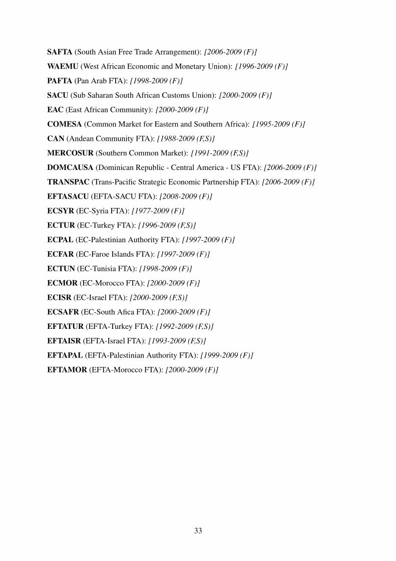
SAFTA (South Asian Free Trade Arrangement): [2006-2009 (F)]

WAEMU (West African Economic and Monetary Union): [1996-2009 (F)]

PAFTA (Pan Arab FTA): [1998-2009 (F)]

SACU (Sub Saharan South African Customs Union): [2000-2009 (F)]

EAC (East African Community): [2000-2009 (F)]

COMESA (Common Market for Eastern and Southern Africa): [1995-2009 (F)]

CAN (Andean Community FTA): [1988-2009 (F,S)]

MERCOSUR (Southern Common Market): [1991-2009 (F,S)]

DOMCAUSA (Dominican Republic - Central America - US FTA): [2006-2009 (F)]

TRANSPAC (Trans-Pacific Strategic Economic Partnership FTA): [2006-2009 (F)]

EFTASACU (EFTA-SACU FTA): [2008-2009 (F)]

ECSYR (EC-Syria FTA): [1977-2009 (F)]

ECTUR (EC-Turkey FTA): [1996-2009 (F,S)]

ECPAL (EC-Palestinian Authority FTA): [1997-2009 (F)]

ECFAR (EC-Faroe Islands FTA): [1997-2009 (F)]

ECTUN (EC-Tunisia FTA): [1998-2009 (F)]

ECMOR (EC-Morocco FTA): [2000-2009 (F)]

ECISR (EC-Israel FTA): [2000-2009 (F,S)]

ECSAFR (EC-South Afica FTA): [2000-2009 (F)]

EFTATUR (EFTA-Turkey FTA): [1992-2009 (F,S)]

EFTAISR (EFTA-Israel FTA): [1993-2009 (F,S)]

EFTAPAL (EFTA-Palestinian Authority FTA): [1999-2009 (F)]

EFTAMOR (EFTA-Morocco FTA): [2000-2009 (F)]

33

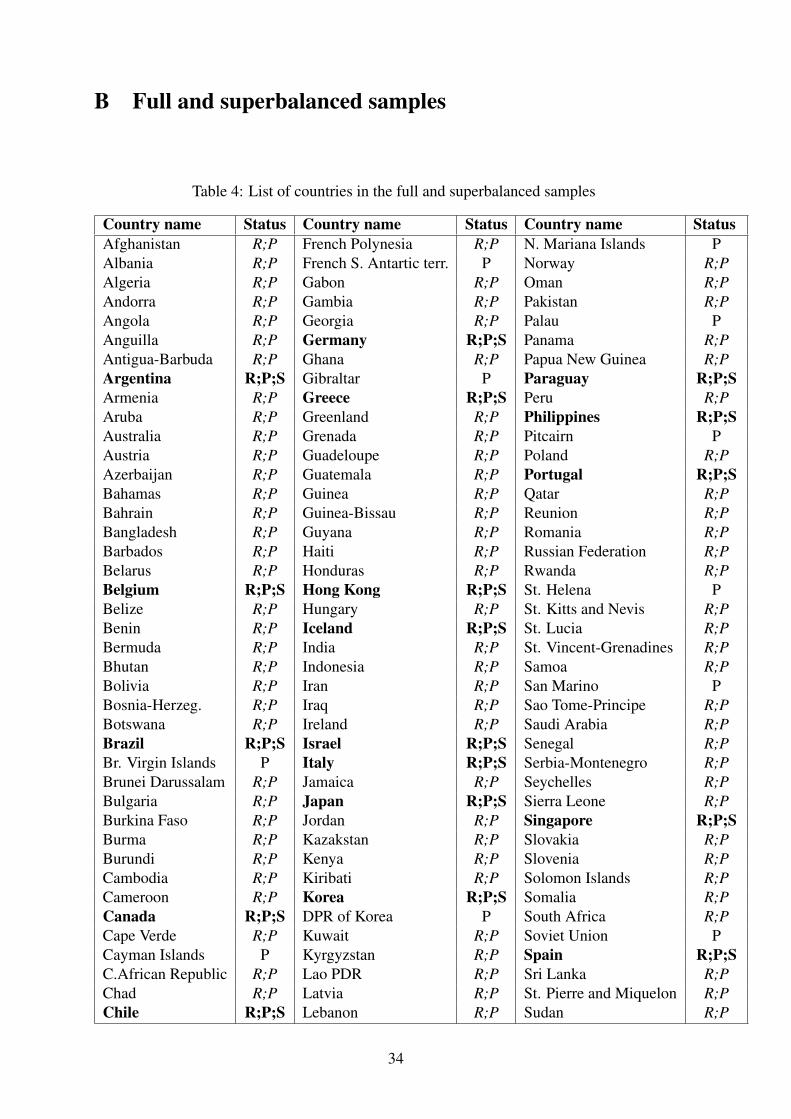
B Full and superbalanced samples

Table 4: List of countries in the full and superbalanced samples

Country name Status Country name Status Country name StatusAfghanistan R;P French Polynesia R;P N. Mariana Islands PAlbania R;P French S. Antartic terr. P Norway R;PAlgeria R;P Gabon R;P Oman R;PAndorra R;P Gambia R;P Pakistan R;PAngola R;P Georgia R;P Palau PAnguilla R;P Germany R;P;S Panama R;PAntigua-Barbuda R;P Ghana R;P Papua New Guinea R;PArgentina R;P;S Gibraltar P Paraguay R;P;SArmenia R;P Greece R;P;S Peru R;PAruba R;P Greenland R;P Philippines R;P;SAustralia R;P Grenada R;P Pitcairn PAustria R;P Guadeloupe R;P Poland R;PAzerbaijan R;P Guatemala R;P Portugal R;P;SBahamas R;P Guinea R;P Qatar R;PBahrain R;P Guinea-Bissau R;P Reunion R;PBangladesh R;P Guyana R;P Romania R;PBarbados R;P Haiti R;P Russian Federation R;PBelarus R;P Honduras R;P Rwanda R;PBelgium R;P;S Hong Kong R;P;S St. Helena PBelize R;P Hungary R;P St. Kitts and Nevis R;PBenin R;P Iceland R;P;S St. Lucia R;PBermuda R;P India R;P St. Vincent-Grenadines R;PBhutan R;P Indonesia R;P Samoa R;PBolivia R;P Iran R;P San Marino PBosnia-Herzeg. R;P Iraq R;P Sao Tome-Principe R;PBotswana R;P Ireland R;P Saudi Arabia R;PBrazil R;P;S Israel R;P;S Senegal R;PBr. Virgin Islands P Italy R;P;S Serbia-Montenegro R;PBrunei Darussalam R;P Jamaica R;P Seychelles R;PBulgaria R;P Japan R;P;S Sierra Leone R;PBurkina Faso R;P Jordan R;P Singapore R;P;SBurma R;P Kazakstan R;P Slovakia R;PBurundi R;P Kenya R;P Slovenia R;PCambodia R;P Kiribati R;P Solomon Islands R;PCameroon R;P Korea R;P;S Somalia R;PCanada R;P;S DPR of Korea P South Africa R;PCape Verde R;P Kuwait R;P Soviet Union PCayman Islands P Kyrgyzstan R;P Spain R;P;SC.African Republic R;P Lao PDR R;P Sri Lanka R;PChad R;P Latvia R;P St. Pierre and Miquelon R;PChile R;P;S Lebanon R;P Sudan R;P

34

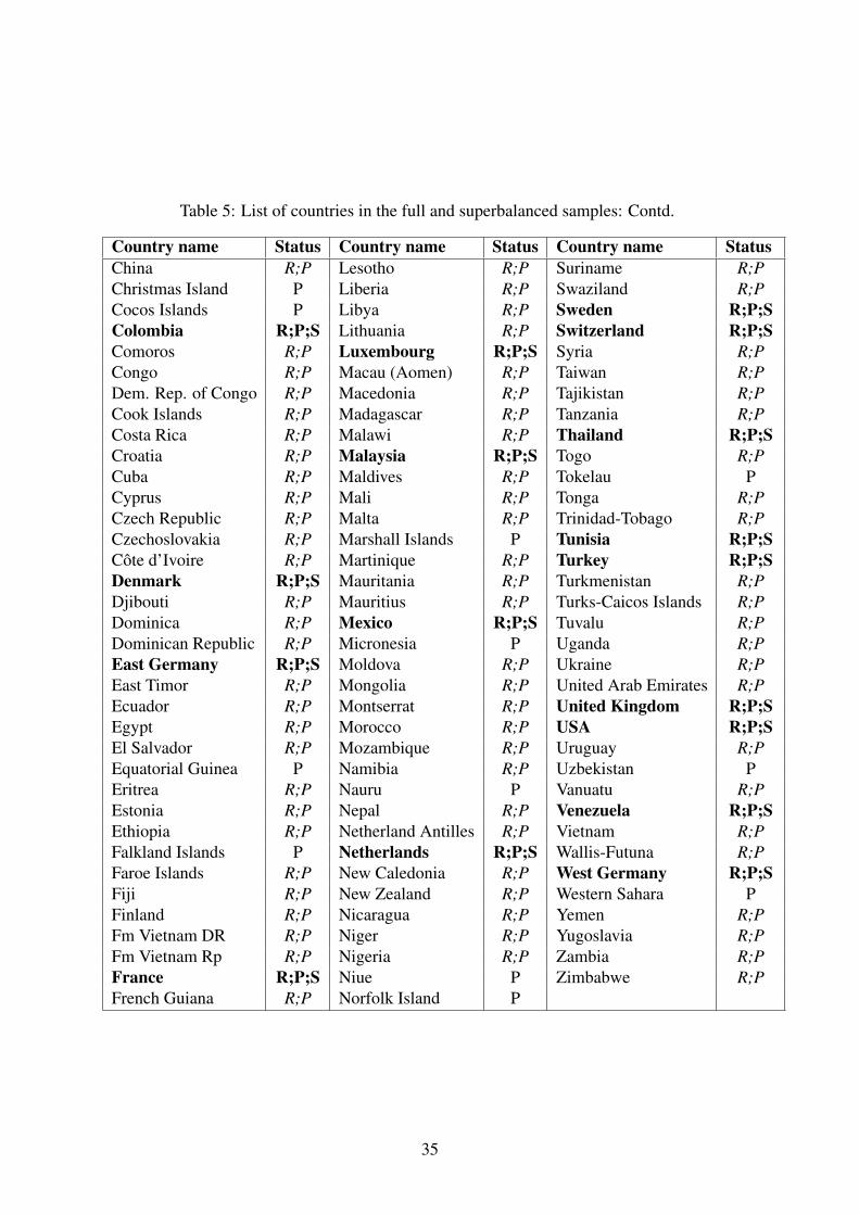
Table 5: List of countries in the full and superbalanced samples: Contd.

Country name Status Country name Status Country name StatusChina R;P Lesotho R;P Suriname R;PChristmas Island P Liberia R;P Swaziland R;PCocos Islands P Libya R;P Sweden R;P;SColombia R;P;S Lithuania R;P Switzerland R;P;SComoros R;P Luxembourg R;P;S Syria R;PCongo R;P Macau (Aomen) R;P Taiwan R;PDem. Rep. of Congo R;P Macedonia R;P Tajikistan R;PCook Islands R;P Madagascar R;P Tanzania R;PCosta Rica R;P Malawi R;P Thailand R;P;SCroatia R;P Malaysia R;P;S Togo R;PCuba R;P Maldives R;P Tokelau PCyprus R;P Mali R;P Tonga R;PCzech Republic R;P Malta R;P Trinidad-Tobago R;PCzechoslovakia R;P Marshall Islands P Tunisia R;P;SCôte d’Ivoire R;P Martinique R;P Turkey R;P;SDenmark R;P;S Mauritania R;P Turkmenistan R;PDjibouti R;P Mauritius R;P Turks-Caicos Islands R;PDominica R;P Mexico R;P;S Tuvalu R;PDominican Republic R;P Micronesia P Uganda R;PEast Germany R;P;S Moldova R;P Ukraine R;PEast Timor R;P Mongolia R;P United Arab Emirates R;PEcuador R;P Montserrat R;P United Kingdom R;P;SEgypt R;P Morocco R;P USA R;P;SEl Salvador R;P Mozambique R;P Uruguay R;PEquatorial Guinea P Namibia R;P Uzbekistan PEritrea R;P Nauru P Vanuatu R;PEstonia R;P Nepal R;P Venezuela R;P;SEthiopia R;P Netherland Antilles R;P Vietnam R;PFalkland Islands P Netherlands R;P;S Wallis-Futuna R;PFaroe Islands R;P New Caledonia R;P West Germany R;P;SFiji R;P New Zealand R;P Western Sahara PFinland R;P Nicaragua R;P Yemen R;PFm Vietnam DR R;P Niger R;P Yugoslavia R;PFm Vietnam Rp R;P Nigeria R;P Zambia R;PFrance R;P;S Niue P Zimbabwe R;PFrench Guiana R;P Norfolk Island P

35

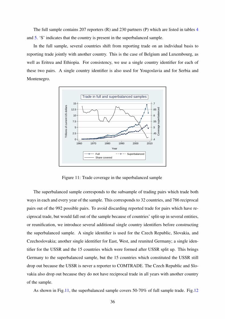
The full sample contains 207 reporters (R) and 230 partners (P) which are listed in tables 4

and 5. ‘S’ indicates that the country is present in the superbalanced sample.

In the full sample, several countries shift from reporting trade on an individual basis to

reporting trade jointly with another country. This is the case of Belgium and Luxembourg, as

well as Eritrea and Ethiopia. For consistency, we use a single country identifier for each of

these two pairs. A single country identifier is also used for Yougoslavia and for Serbia and

Montenegro.

.4

.45

.5

.55

.6

.65

.7

Cov

erag

e su

perb

alan

ced

0

2.5

5

7.5

10

12.5

15

Tril

lions

of c

urre

nt U

S d

olla

rs

1960 1970 1980 1990 2000 2010

Year

Full SuperbalancedShare covered

Trade in full and superbalanced samples

Figure 11: Trade coverage in the superbalanced sample

The superbalanced sample corresponds to the subsample of trading pairs which trade both

ways in each and every year of the sample. This corresponds to 32 countries, and 786 reciprocal

pairs out of the 992 possible pairs. To avoid discarding reported trade for pairs which have re-

ciprocal trade, but would fall out of the sample because of countries’ split-up in several entities,

or reunification, we introduce several additional single country identifiers before constructing

the superbalanced sample. A single identifier is used for the Czech Republic, Slovakia, and

Czechoslovakia; another single identifier for East, West, and reunited Germany; a single iden-

tifier for the USSR and the 15 countries which were formed after USSR split up. This brings

Germany to the superbalanced sample, but the 15 countries which constituted the USSR still

drop out because the USSR is never a reporter to COMTRADE. The Czech Republic and Slo-

vakia also drop out because they do not have reciprocal trade in all years with another country

of the sample.

As shown in Fig.11, the superbalanced sample covers 50-70% of full sample trade. Fig.12

36

shows the distribution of pairs in the full sample according to the number of years they are

present in the sample.

0.0

1.0

2.0

3.0

4.0

5D

ensi

ty

0 10 20 30 40 50Number of years

Pair presence in 1962−2009

Figure 12: Number of years each pair is present in the sample

As a check on the way the superbalanced sample is constructed, we redefine the set of pairs

which trade both ways in each year starting from 1970, e.g. the first year in which there are more

than 100 reporters in the COMTRADE database.41 This gives a sample of 1604 reciprocal pairs

out of the 2162 possible pairs for 47 reporters (partners). Fig.13 shows that evolution of trade

coverage is qualitatively similar.

Fig.14 shows the share of total trade covered by pairs which traded both ways in 1962, and

as a check, the share of total trade by pairs which traded both ways in 1970. Qualitatively, trade

coverage is similar to the superbalanced samples for, respectively, 1962 (1970). In the same

figure, it is shown that one-way trade flows represent a marginal and decreasing share of world

trade: more than 95% of total annual trade takes place between pairs which trade both ways in

that year. This finding is complementary to Helpman et al. (2008) who find that the increase in

world trade is driven by pairs which trade both ways in 1970. Helpman et al. (2008) find that

the enlargement of the set of trading partners did not contribute in a major way to the growth

of world trade in 1970-1997. We nuance this finding by showing that trade between partners

who did not trade both ways in 1962 (1970) did contribute strongly to the increase in total

trade in 1995-2009. Furthermore, these new trade relationships were formed between countries

trading both ways. Part of the explanation of the widening gap between the superbalanced and

41 There are 71 reporters in 1962, and 112 in 1970.

37

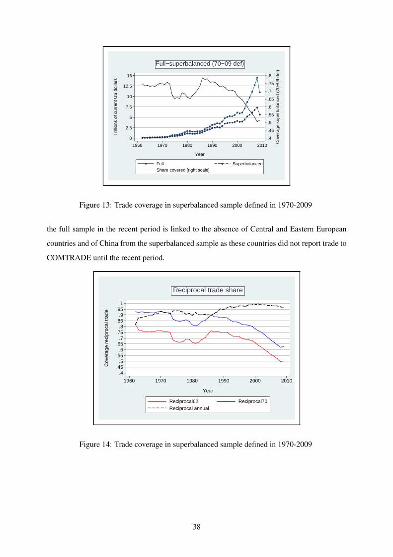
.4

.45

.5

.55

.6

.65

.7

.75

.8

Cov

erag

e su

perb

alan

ced

(70−

09 d

ef)

0

2.5

5

7.5

10

12.5

15

Tril

lions

of c

urre

nt U

S d

olla

rs

1960 1970 1980 1990 2000 2010

Year

Full SuperbalancedShare covered [right scale]

Full−superbalanced (70−09 def)

Figure 13: Trade coverage in superbalanced sample defined in 1970-2009

the full sample in the recent period is linked to the absence of Central and Eastern European

countries and of China from the superbalanced sample as these countries did not report trade to

COMTRADE until the recent period.

.4.45.5

.55.6

.65.7

.75.8

.85.9

.951

Cov

erag

e re

cipr

ocal

trad

e

1960 1970 1980 1990 2000 2010

Year

Reciprocal62 Reciprocal70Reciprocal annual

Reciprocal trade share

Figure 14: Trade coverage in superbalanced sample defined in 1970-2009

38

C Robustness checks for instrumented prices

This appendix shows that our results on the evolution of the substitutability parameter in the

estimation with instrumented prices are robust to increasing the number of periods s for which

the growth rate in the relative price of the exported composite good is predicted on the evolution

of relative domestic prices.

Fig.(15) shows that, as we increase s from 3 to 5, the evolution of the estimated substi-

tutability parameter becomes steeper, and the increase in the level of the parameter becomes

more stable across the years. Thus, for s = 5, the parameter is found to increase by 18% in

1967-2009 while its level increases by 20% on average relatively to the estimate obtained with

observed relative prices.

−.9

−.8

−.7

−.6

−.5

−.4

1960 1970 1980 1990 2000 2010year

coef_elast_p_L3 coef_elast_p_L5

linear fit L3 linear fit L5

Trade elasticity (instrumented relative price, 3 and 5 lag)

Figure 15: Estimated (1− σ̃), instrumented relative price of composite good

For s = 10, the substitution elasticity increases by 29% in 1972-2009, and the absolute

value of the parameter increases by 22% on average relatively to the estimate obtained with

non-instrumented prices.

39