The Forward Discount Puzzle: Identification of Economic

Assumptions

Seongman Moon∗ Carlos Velasco†

Universidad Carlos III de Madrid Universidad Carlos III de Madrid

January 4, 2011

Abstract

The forward discount puzzle refers to the robust empirical finding that

foreign excess returns are predictable. We investigate if expectations errors

are the main cause of this predictability using the serial dependence pattern

of excess returns implied by economic models as identification device. This

approach also allows us to explain why strong predictability of excess re-

turns only occurs during 1980s. Using USD bilateral spot and forward rates

from 1975-2009, we show that both the statistically significant positive serial

dependence of excess returns in the entire sample and the very weak (mostly

insignificant) positive serial dependence in the subsample excluding obser-

vations in 1980-87 are consistent with the predictions of the expectations

errors explanation. We provide several pieces of new empirical evidence

which support the link between the strong predictability in the 1980s and

changes in forecasting techniques by foreign exchange market agents.

Keywords: expectations errors, rational expectations risk premium, excess returns,serial dependence, 1980-87.

JEL Classification: F31, G14.

∗Department of Economics, Universidad Carlos III de Madrid, Calle Madrid 126, 28903 GetafeMadrid, SPAIN. Email: smoon@eco.uc3m.es, Tel.: +34-91-624-8668. Research support from theSpanish Plan Nacional de I+D+I (SEJ2007-63098) is gratefully acknowledged.

†Department of Economics, Universidad Carlos III de Madrid, Calle Madrid 126, 28903 GetafeMadrid, SPAIN. Email: Carlos.Velasco@uc3m.es, Tel.: +34-91-624-9646. Research support fromthe Spanish Plan Nacional de I+D+I (SEJ2007-62908) is gratefully acknowledged.

1

1 Introduction

The unbiased hypothesis of forward exchange rates states that the forward rate

is the optimal predictor of future spot rates and implies that the expected excess

return on foreign relative to domestic currency must be zero. However, numerous

studies have persistently documented that excess returns are predictable, mainly

using the forward discount or past returns as predictors. The forward discount

puzzle, one of the most robust puzzles documented in international economics,

refers to such findings.1

There have been two popular explanations for the forward discount puzzle in

the literature: rational expectations risk premia and expectations errors.2 We

reconsider these explanations and investigate the following questions: (i) Is the

predictability due to the presence of the time-varying risk premium in an efficient

market or evidence of market inefficiency which reflects deviations from strong

rationality?3 (ii) Why does the strong predictability only appear in the 1980s?

Froot and Frankel (1989) first addressed this identification issue using addi-

tional data such as survey data. Instead, we look for information directly from the

economic model that restricts the relations between the behavior of macro funda-

mentals and equilibrium expected returns. We pay particular attention to the se-

rial dependence pattern of excess returns over return horizons implied by economic

models for the expected excess returns. We argue that empirical evidence on this

serial dependence pattern provides a valid criterion for judging the performance

of economic models. The main argument is that a mean reverting component in

excess returns, representing a violation of the unbiased hypothesis, can generate

different serial dependence patterns, depending on the economic model assump-

tions. On the one hand, a class of rational expectations risk premium models tends

to generate ‘negative’ serial dependence in excess returns mainly because funda-

mental variables are negatively correlated with the risk premium in these models,

1See, Lewis (1995) and Engel (1996) for the survey. For recent contributions, see Chinn(2006).

2Several studies also investigate poor finite sample properties of predictive regression tests[see, for example, Evans and Lewis (1995)]. In a recent paper, Bacchetta and van Wincoop(2010) present another explanation based on the model of infrequent portfolio decisions.

3For example, Alvarez, Atkeson, and Kehoe (2009) and Verdelhan (2010) are successful forrelating the cause of the forward discount puzzle to the rational expectations risk premium. Onthe other hand, Froot and Frankel (1989), Frankel and Froot (1990a, 1990b), Mark and Wu(1998), and Gourinchas and Tornell (2004) related successfully the cause to expectations errors.

2

e.g., counter-cyclical exchange risk premia in Verdelhan (2010). Those include a

monetary general equilibrium model with time varying risks by Alvarez, Atkeson,

and Kehoe (2009) and an external habit-persistence model with time-varying risk

aversion by Verdelhan (2010), which are successful in generating highly variable

risk premia. On the other hand, a class of models for expectations errors tends to

generate ‘positive’ serial dependence in excess returns. Those include a model of a

speculative bubble by Frankel and Froot (1990a, 1990b) and a noise trader model

by Mark and Wu (1998).

Our analysis also complements the popular criterion on the performance of

economic models in the literature. In order to investigate the influence of the

risk premium in foreign exchange markets, studies have focused on whether or

not their models can generate a variance of the risk premium higher than that of

the expected exchange rate change. This volatility relation was first illustrated

by Fama (1984) using the decomposition of the slope coefficient in the regression

of the exchange rate change on the forward discount. However, several studies

show that the estimated slope coefficient may not be so informative because its

distribution is very wide and the magnitude of systematic estimation errors can be

large (see, e.g., Baillie and Bollerslev (2000), West (2008), and Moon and Velasco

(2010b)). We also present empirical findings which support this conclusion and

argue that previous studies may have overemphasized the estimation results from

Fama regression. By contrast, our approach is not subject to this shortcoming,

identifies the predictability over return horizons, and provides an explicit criterion

for the judgement on the model performance.

Using US dollar (USD) bilateral spot and one-, three-, six- and twelve-month

forward rates from 1975-2009, we find that excess returns strongly exhibit posi-

tive serial dependence over return horizons up to five years, consistent with the

prediction of the expectations errors explanation. But the predictability of excess

returns becomes very weak in the sample which excludes observations in 1980-87:

excess returns are not statistically significant in most currencies, implying that

the deviations from the unbiased hypothesis are mainly driven by a particularly

influential subset of the data.

This evidence leads us to investigate the second question and to reconsider the

speculative bubble hypothesis on the path of the US dollar in the 1980s proposed by

3

Frankel and Froot (1990a, 1990b). In particular, we link our empirical results with

‘changes in forecasting techniques’ used by agents in foreign exchange markets

in the 1980s. That is, by assuming that the market expectation is a weighted

average of expectations of fundamentalists and chartists, we relate the changes

in the weights during 1980s to the market’s Bayesian responses to the relative

forecasting performance of an agent. We also provide several pieces of evidence

which support this argument: (i) the very strong predictability of excess returns

in 1980-87 is only observed in USD bilateral rates; and (ii) the behavior of the

survey expectation is consistent with the market expectation over both subsample

periods: when the unbiased hypothesis is decisively rejected and also when it tends

to hold.

The organization of the paper follows. Section 2 documents empirical results

on the strong predictability of excess returns in the 1980s based on the standard

regression tests. Section 3 shows analytically that the two competing economic

explanations generate an opposite sign of the serial dependence in excess returns.

Section 4 provides empirical results on the serial dependence pattern of excess

returns based on the variance ratio test. Section 5 offers an explanation for the

appearance of strong predictability in the particular sample period of 1980-87 and

Conclusions follow.

2 Strong Predictability of Foreign Excess Returns in the 1980s

We perform the predictability test on one-, three-, six- and twelve-month excess

returns based on the following standard regression for currency excess returns,

st+k − ft|k = αk + βk(ft|k − st) + ut+k, (1)

where st denotes the log of the domestic currency price of foreign currency at time t

and ft|k denotes the log of the domestic currency price at time t of foreign currency

delivered at t+k. Both αk and βk are zero for any k under the unbiased hypothesis

with the assumptions of rational expectations and risk neutrality. Under these

assumptions, the unbiased hypothesis is equivalent to the uncovered interest parity

(UIP) hypothesis. From now on, we use both hypotheses interchangeably. Our

sample consists of weekly observations of eleven London close mid prices whose

description is presented in Table I.

4

2.1 Standard Results Reproduced

Table III reports the estimated slope coefficients both when regression (1) is

estimated for an individual currency and when a single β is estimated for a pooled

sample of all currencies and periods of time as well as for two portfolios which

consist of five major currencies: the German mark (GDM), the British pound

(BRP), the Japanese yen (JPY), the Canadian dollar (CAD), and the Swiss franc

(SWF). The first portfolio (Eport) is constructed using an equal weight and the

second one (Wport) is constructed based on weights calculated using the data of

foreign exchange market turnover by currency pair.

Panel A provides the results from the entire sample period. Consistent with

the previous empirical findings, β̂k are negative (mostly less than -1) and the

conventional t-test rejects the UIP hypothesis at a 1% level in almost all cases.

For example, the pooled β̂k are -1.06, -1.04, -0.97, and -0.88, respectively, for the

one-, three-, six-, and twelve-month maturities and statistically significant at all

the conventional levels. Notoriously, the R2s in the regressions are very low in

magnitude. These results confirm well-known empirical regularities, which refer

to the forward discount puzzle.

2.2 Strong Predictability in the 1980s

We now conduct the same predictive test on subsample periods. In particular,

we are interested in conducting the test on the sample which excludes observations

of 8 years in the period of 1980-87, out of 35-year observations in the entire sample.

The separation is motivated by empirical evidence on the predictability of excess

returns in the 1980s. For example, studies often find ambiguous results using

observations in the 1990s, although salient deviations from UIP are detected based

on the data before 1990s [see, e.g., Flood and Rose (2002)]. Evans (1986) and

Meese (1986) also provide evidence on the presence of speculative bubbles in foreign

exchange markets during the first half period of the 1980s.

Panel B reports the results from regression (1) using the sample excluding ob-

servations in 1980-87. From now on, we call it subsample E. In contrast to the

results in the entire sample, the UIP hypothesis tends to hold or the rejections

become very weak. The t-test does not reject it for most currencies: β̂k is sta-

tistically indistinguishable from zero at a 5% level in most cases. For example,

5

the t-statistics of the pooled estimates are -1.64, -1.51, -1.50, and -1.57, respec-

tively, for the one-, three-, six-, and twelve-month maturities. Both portfolios also

produce similar results except for the twelve-month maturity: the estimates are

marginally rejected at the 5% level. For individual currencies, the rejections only

occur at the 5% level for CAD and the Australian dollar (AUD) for the one-month

maturity, and for CAD and the Danish Krone (DAK) for the three-month matu-

rity. For other maturities, the rejection only occurs for JPY for the twelve-month

maturity. We find some more rejections at the 10% level for the six- and twelve-

month maturities. These results are surprising, compared to those from the entire

sample as well as from numerous previous studies.

The results using another subsample which contains observations only in 1980-

87 [We call it subsample O] are reported in Panel C and further confirm that

the rejections in the entire sample seem to be significantly influenced by this.

The absolute values of both the estimated slope coefficients and their t-statistics

are much greater than those in the other sample periods. Further, the strong

explanatory power of the forward discount, measured by R2, is noticeable.4 For

example, for BRP, the R2s are 0.18, 0.43, 0.52, and 0.36 for the one-, three-, six-,

and twelve-month maturities, respectively, while they are almost zero in subsample

E, indicating that the strong negative correlation between the spot return and

the forward discount may be only present in this particular sample period.5 This

pattern appears for most major currencies. Our findings are, in a sense, compatible

with numerous previous studies that document the strong predictability of excess

returns simply because their samples include observations in the 1980s.

2.2.1 Robustness I: A Parameter Stability Test

For the robustness, we first investigate if the above results are sensitive to

the selection of the subsample period. For this, we design a stability test based

4For the one-month and three-month maturities, we also calculate R2 using non-overlappingobservations to see if the results are contaminated by overlap of the data. However, they arerobust to this change.

5Our empirical findings can be related to those of Bansal (1997). He found that deviationsfrom the UIP hypothesis depend systematically on the sign of the interest rate differential acrosscountries using weekly data of GDM and JPY in 1981-95. Specifically, the US dollar was stronglyappreciated when the US interest rate was greater than other countries’ interest rates but UIPtends to hold when it is less than them. According to our data, the US interest rate was higherthan others for most weeks during the time period of 1981-85.

6

on rolling samples, instead of typical ones using cumulated sample observations.6

We generate 8-year rolling samples whose size is equal to that of subsample O.

The first sample is obtained using weekly observations on each country’s spot and

one-month forward rates from January 1975 to December 1982. The next sample

then contains those from January 1976 to December 1983, that is, observations in

1975 are dropped and those in 1983 are added. And so on. We estimate the slope

coefficient in regression (1) for each rolling sample j for j = 1, . . . , J and obtain

its t-statistic. To estimate critical values for the tests on the stability of βk, we

use a bootstrap algorithm specified in detail in Appendix A.

Figure 1 plots the locus of the t-statistics obtained using 8-year rolling samples

as well as the 90% uniform test bands with 5 and 95% quantiles from the simulated

bootstrap empirical distribution of t-statistics. We reject the null hypothesis that

all the slope coefficients in rolling samples of one-month excess returns are zero at

the 10% significance level for all five major currencies considered. However, the

rejections are mainly due to rolling samples which include some observations in

the period of 1980-87. In those samples, the estimates are significantly negative

and the corresponding t-statistics are much beyond the lower bound of the 90%

band. On the other hand, the t-statistics from rolling samples which do not contain

observations in 1980-87 tend to be inside the band. These confirm the empirical

results that the predictability of excess returns is very weak in subsample E.

2.2.2 Robustness II: Statistical Issues

We now examine the extent of possible statistical artifacts. In particular, we

are concerned about the sensitivity of statistical inference: the t-statistics can

change dramatically with the drop/addition of a few observations when the re-

gressor is highly persistent, as discussed in Campbell and Yogo (2006). Therefore,

we investigate if the difference in the results between the two samples with/without

observations in 1980-87 can be attributable to problems in the specification of the

persistency.7

6We thank Efstathios Paparoditis for the suggestion of this method. Baillie and Bollerslev(2000) also generate rolling samples to investigate the pattern of the slope coefficient in theregression of spot rates on the forward discount.

7Similarly, several studies (e.g., Baillie and Bollerslev (2000), and Maynard and Phillips(2001), and references therein) are concerned with the over-rejections of regression tests usingconventional critical values, based on empirical evidence on the (near) nonstationary behavior ofthe forward discount.

7

For this, we conduct the conditional test developed by Jansson and Moreira

(2006) based on the regression model in equation (1) because their test has correct

size and desirable power properties in the specification with (near) integrated re-

gressors.8 For implementing the test, we follow Polk, Thompson, and Vuolteenaho

(2006) who apply the same test for stock return predictability.9 The test is con-

ducted based on the samples with non-overlapping observations since it cannot

account for serial dependence in predictive errors. We choose observations at the

end of each maturity, for example, at the end of each month for the one-month

maturity.

Table IV reports the t-statistics of the estimated slope coefficient in regression

(1) and 2.5 and 97.5% quantiles of the conditional t distribution. We find that

both the conventional t-test and the conditional test produce quite similar results:

both tests agree with the rejections/non-rejections. And the critical values at the

two quantiles obtained from the conditional test are quite similar to those from the

conventional t-test. For example, both tests decisively reject the null hypothesis

in the entire sample for most currencies. On the other hand, they do not reject

it for most currencies in subsample E. These results suggest that a statistical

phenomenon cannot be the reason for our empirical findings.10 As Mankiw and

Shapiro (1986) illustrate, the conventional t-test over-rejects the null in regression

(1) if the contemporaneous correlation between innovations to the regressor and

to the dependent variable is large and the regressor is strongly persistent. In our

sample, the forward discount is highly persistent [see Table 2], while the contem-

poraneous correlations are close to zero. For example, the absolute values of the

correlations are less than 0.1 for all currencies, suggesting that the absence of sta-

tistical distortions may be due, at least partially, to the small contemporaneous

correlations.

8We also conduct Campbell and Yogo’s Q test and find that the results are quite similarbetween the two tests. For the sake of simplicity, we do not report those from the Q-test.

9We use the Matlab codes written by Polk, Thompson, and Vuolteenaho (2006) with a smallmodification for our study. Their codes are available athttp : //personal.lse.ac.uk/POLK/research/work.htm.10Our results are consistent with Maynard (2006) who studied the effects of a statistical phe-

nomenon in foreign exchange markets.

8

2.3 Information in the Estimated Slope Coefficients

In this subsection, we discuss the precision of the estimated slope coefficient as

well as the magnitude of the estimation bias. One apparently peculiar phenomenon

regarding the results from subsample E is that the sign of the estimated slope

coefficients is towards a particular direction, although they are not statistically

significant and there is no clear symptom of statistical distortions. Estimates are

negative for all cases and less than -1 for many cases. If the distribution of the

estimated slope coefficient were normal, then on average we should observe both

positive and negative values equally likely.

We argue that this can be explained by the typical present value models. Specif-

ically, Moon and Velasco (2010b) show that it may not be uncommon to observe

‘insignificant’ estimates with large deviations from the null value and with the

same sign, based on the bivariate regression in which both st and ft|k are gener-

ated under the UIP hypothesis.11 The key idea can be seen in the decomposition

of the contemporaneous correlation, γ,

γ =σuv/σ

2v

σu/σv, (2)

where σu is the standard deviation of the error term ut+1 in regression (1) and σv is

the standard deviation of the error term in the regression of the forward discount

on its lagged value. The scale factor, σuv/σ2v , affects the magnitude of the bias,

E[β̂ − β], in regression (1) [see, e.g., Stambaugh (1999)] and the noise-to-signal

ratio, σu/σv, mainly determines the variance of the estimated slope coefficient, β̂.

Equation (2) shows that a large magnitude of the bias must be accompanied by a

large value of σu/σv and thus of the standard error of β̂, since the absolute value of

γ is bounded by one. However, a smaller correlation of γ is not necessarily related

to a smaller value of σu/σv. In an extreme case, σu/σv can take any value if σuv is

zero. Equation (2) also implies that a large magnitude of bias does not necessarily

lead to significant over-rejections of the t-test. Rather, what matters is the ratio

between σuv/σ2v and σu/σv, which determines the standardized bias of the t-test.

Moon and Velasco (2010b) show that, in the present value models, the near unit

values of the discount factor and the persistence parameter induce a larger value of

σu/σv as well as a larger magnitude of bias and thus a wider distribution of β̂, while

11See, also, Baillie and Bollerslev (2000) and West (2008) who reached a similar conclusion onthe information content of the estimated slope coefficient.

9

generating a smaller value of the contemporaneous correlation. Consequently, the

estimated slope coefficient becomes less informative and, at the same time, the

over-rejections do not occur. Empirical evidence on the large values of the discount

factor [see, e.g., Engel and West (2005)] and on strong persistence in the forward

discount [see Table 2] supports this argument. Further, the large magnitude of

σu/σv is consistent with the foreign exchange data in that the relative variance

between the excess return and the forward discount is in general very large. For

example, for the one-month maturity, the relative variances between the two series

are in general greater than 150 for most currencies as in Table 2.

This result may challenge the conventional view on Fama (1984)’s volatility

relation which has been used as one of the criteria for evaluating the performance

of the rational expectations models in terms of generating high volatilities of the

risk premium. Since the relation is derived from the magnitude of β̂, it is important

to understand if the estimates contain valid information. In the next section, we

provide an alternative identification strategy which may complement this volatility

relation.

3 Identification of Two Competing Explanations: RationalExpectations Risk Premia vs. Expectations Errors

In this section, we consider an implication of general models for the expected

excess returns: the serial dependence pattern of excess returns. In particular, we

use as an identification device the sign of autocorrelations of excess returns which

is critically determined by a feedback from forecasting errors to future expected ex-

cess returns. To illustrate this, we present the two well-known explanations for the

predictability of excess returns, rational expectations risk premia and expectations

errors, and show that they tend to generate opposite signs of the autocorrelation

function of those returns.

3.1 An Exchange Rate Model

Following Frankel and Froot (1990b) and Engel and West (2005), we consider

a general setup for the determination of the exchange rate

st = αEt[∆st+1] + αpet − αpt +ϖt + wt, (3)

10

where pet = Emt [∆st+1]−Et[∆st+1] is the difference between the market expectation

and the rational expectation (expectations errors), pt is the risk premium, ϖt is

the log of the real exchange rate, wt is the linear combination of logs of other

fundamental variables such as money and output, and α is constant. ϖt represents

a deviation from the log of purchasing power parity (PPP), while both pet and pt

represent deviations from the log of UIP,

Et[∆st+1] + pet − pt = it − i∗t = ft − st (4)

where the second equality represents the log of covered interest parity. We assume

maturity k = 1 in this section and omit the notation for maturity, for example

we denote the log of the one-period forward exchange rate by ft = lnFt|1. In the

typical monetary models, equation (3) is derived from home and foreign money de-

mands combined with equation (4) [see, e.g., Engel and West (2005) and Obstfeld

and Rogoff (2002) for the rational expectations and Frankel and Froot (1990b) for

the expectations errors models].

We assume that the process for wt follows

∆wt = ρ∆wt−1 + ηt, (5)

where ηt represents a stochastic disturbance with mean zero and variance σ2η. If

ρ = 0, then the fundamental process follows a random walk. The introduction of

more complicated fundamental processes would not change our main results below

mainly because the predictability of excess returns is coming from deviations from

UIP. Therefore, considering equation (5) may be enough for our objectives.

For modeling the rational expectations risk premium, we begin with considering

currency prices in a fairly general setting and then turning to more structured

economies. On the other hand, we follow Frankel and Froot (1990b) for modeling

expectations errors. Both pt and pet are assumed to follow a stationary process,

respectively, as specified in detail below. With these assumptions and ρ = 0,

the spot exchange rate can be described by the combination of a random walk

fundamental and some persistent stationary components due to the deviations

from UIP, mirroring a well-known fads model used for studying the predictability

of stock returns in Fama and French (1988) and Poterba and Summers (1988).

11

3.2 Rational Expectations Risk Premia

In this subsection, we identify the influence of the time-varying rational ex-

pectations risk premium on the return predictability. For this, we consider three

different risk premium models. One is a general equilibrium sticky-price mone-

tary model [see, e.g., Obstfeld and Rogoff (2002)]; another is a general equilibrium

monetary model with an endogenous source of risk variation by Alvarez, Atkeson,

and Kehoe (2009); the other is an external habit persistence model by Verdelhan

(2010). Considering our objectives, we mainly derive the equilibrium (expected)

excess returns from the first model as a benchmark and relegate the presentation

of the latter two models to the technical and empirical appendix. Nevertheless,

we discuss the key mechanisms and assumptions of all three models to identify the

link between the time series behavior of the risk premium and the sign of serial

dependence of excess returns. We begin with deriving the risk premium from a

currency pricing setting whose definition is exactly applied to all the three models.

Assume that there are no arbitrage opportunities in an economy so that a

pricing kernel exists. Let mt+1 be the pricing kernel for home (dollar) assets and

m∗t+1 be the pricing kernel for foreign (euro) assets. These pricing kernels imply

that any asset purchased in period t with a dollar excess return of Rt+1 between

periods t and t+ 1 and any asset purchased with a euro return of R∗t+1 satisfy the

Euler equations, respectively,

1 = Et[mt+1Rt+1], 1 = Et[m∗t+1R

∗t+1]. (6)

In the complete asset markets, there exist unique m and m∗ that satisfy equation

(6). Although the pricing kernels are not unique in the incomplete asset markets,

they can be chosen to satisfy the same equations [see, for example, Backus, Foresi,

and Telmer (2001, Proposition 1)]. So, the pricing kernel for home assets, mt+1,

can be related to m∗t+1 in the following way,

m∗t+1 =

mt+1St+1

St

. (7)

Analogously, the log of the price of a one-period dollar-denominated bond and

that of a one-period euro-denominated bond can be expressed as

it = − logEt[mt+1], i∗t = − logEt[m∗t+1] (8)

where it (i∗t ) is the home (foreign) nominal interest rate.

12

Taking logs of equation (7) and then conditional expectations on a time t

information set, and using the expressions for the nominal interest rates as well as

the log of covered interest parity, we can define the foreign exchange risk premium,

pt, by12

pt = Et[st+1]− ft = (lnEt[mt+1]− Et[lnmt+1])− (lnEt[m∗t+1]− Et[lnm

∗t+1]). (9)

If both mt+1 and m∗t+1 follow a conditional log normal distribution, then

pt =1

2(V art[lnmt+1]− V art[lnm

∗t+1]). (10)

We now consider the reduced-form expression for the foreign exchange risk

premium premium, assuming that it follows an univariate AR(1) process,

pt = (1− φ)µϵ + φpt−1 + ϵt, (11)

where 0 < φ < 1 and ϵt is an iid random variable with mean zero and variance

σ2ϵ . We follow this simplifying assumption on the process for pt since it mimics the

process of the risk premium endogenously driven from the economic models. We

also present the reduced form expression for the foreign excess returns, ret+1,

ret+1 = st+1 − ft = fdt+1 + fpt+1 + pt, (12)

where constant terms are omitted for simplicity. The first two terms in the right-

hand side of equation (12) are rational forecasting errors which contain two dis-

turbance terms: fdt+1 is from the fundamental process and fpt+1 is from the risk

premium process. For example, fdt+1 is the difference between disturbances to

home and foreign money growth rates in Obstfeld and Rogoff (2002) and Alvarez,

Atkeson, and Kehoe (2009) and the difference between disturbances to home and

foreign consumption growth rates in Verdelhan (2010).13 Equation (12) implies

that the forecasting errors between time t and t + 1 will be correlated with the

future values of pt, which provides an identification device for the sign of autocor-

relations of excess returns.12Two popular definitions for the risk premium are interchangeably used in the literature. For

example, several studies define the risk premium by pt = Et[st+1] − ft like us [e.g., Alvarez,Atkeson, and Kehoe (2009) and Verdelhan (2010)], while the other studies define it by pt =ft − Et[st+1] [e.g., Froot and Frankel (1989), Engel (1996), Backus, Foresi, and Telmer (2001),and Obstfeld and Rogoff (2002)]. However, this would not change the result because the sign ofpt in equation (4) will change accordingly.

13Verdelhan abstract from money and inflation and focuses on real risk. So, the currencyexcess return in equation (12) should be interpreted accordingly.

13

The covariance of two consecutive ex post excess returns between t + 1 and

t+ 2 is

Cov(ret+1, ret+2) = Cov(fpt+1, pt+1) + φV ar(pt) + σηϵ, (13)

where σηϵ = Cov(fdt+1, ϵt+1) captures the relation between shocks to the funda-

mental value and shocks to the risk premium.14 Although the sign of σηϵ is model

specific, the three models considered generate either a negative sign or a zero cor-

relation. For example, Alvarez, Atkeson, and Kehoe (2009) built a model which is

driven by exogenous shocks to the growth rates of money supply in each country

(the difference between home and foreign money supply in their model can be in-

terpreted as the economic fundamental, w, in our setup). They show that a change

in the home money growth rate is negatively related to pt if the money growth rate

is persistent and uncorrelated with pt if the money growth rate is iid, i.e., ρ = 0

in our setup [see their equation (39)]. On the other hand, Verdelhan (2010) built

an external habit persistent model which is driven by exogenous iid shocks to the

growth rates of consumption in each country (the difference between home and

foreign consumption in their model can be interpreted as the economic fundamen-

tal, w, with ρ = 0, in our setup). His model also generates the negative sign of

σηϵ, implying counter-cyclical risk premia. As shown in the technical and empir-

ical appendix, the negative sign of σηϵ is one of the key conditions that generate

negative autocorrelations of excess returns in the risk premium models considered.

We also find that the sign of Cov(fpt+1, pt+1) is either negative or zero in all three

models. For example, the negative sign of Cov(fpt+1, pt+1) can be easily checked

from equations (3) and (4) in the typical monetary models such as Obstfeld and

Rogoff (2002). Alvarez, Atkeson, and Kehoe (2009) impose that exchange rate

follows a random walk in their calibration, implying that the covariance is zero.

We now examine the behavior of the foreign excess return over long horizons

since it also provides information on the importance of the risk premium in ex-

change rates [see, e.g., Fama and French (1988)]. This can be easily seen in the

following covariance between ret+1 and ret+1+q for q ≥ 1

Cov(ret+1, ret+1+q) = φq−1Cov(ret+1, r

et+2), (14)

where φq−1 summarizes the long-horizon predictability of the excess return. Equa-

14Campbell (1991) also derives this expression from the present value of stock prices with theexpected return process (11).

14

tion (14) shows that the sign of Cov(ret+1, ret+1+q) is the same as that of Cov(ret+1, r

et+2)

and the predictability of excess returns will die out eventually. As Fama and

French (1988) shows, the accumulation of these autocovariances can induce strong

autocorrelations over long horizons, which may not be clearly captured over short

horizons. Therefore, examining the pattern of autocorrelations of excess returns

over long horizons can take a clearer picture of the importance of a mean reverting

component in exchange rates, which is the deviation from UIP.

To see explicitly the relative magnitude among the three quantities in Cov(ret+1, ret+2),

we need to resort on a specific economic model. As an example, we calculate the

autocorrelation of the excess return based on the model by Obstfeld and Rogoff

(2002) with the modification on their assumption of the money supply process,

while relegating our analysis on the other models to the technical and empirical

appendix. Obstfeld and Rogoff assume that money supply in each country fol-

lows a random walk, that is, ρ = 0, in our setup. They further assume that the

shocks to the money growth rates are time invariant so that the risk premium is

constant. To make it time varying, we assume that the distribution of the money

growth rates follows an ARCH process so that we can assume (11) for the risk

premium process in the spirit of Abel (1988) and Hodrick (1989). In particular,

from equations (3)-(5) and (11), we have

fdt+1 = ηt+1, fpt+1 = − b

1− bφϵt+1. (15)

Then, from equations (13) and (15), we have

Cov(fdt+1, pt+1) = 0, Cov(fpt+1, pt+1) + φV ar(pt) =φ− b

(1− bφ)(1− φ2)σ2ϵ . (16)

Equation (16) shows that the sign of Cov(fpt+1, pt+1)+φV ar(pt) depends only on

two parameter values: if the discount factor is less than φ, then it is positive; if the

discount factor is greater than φ, then it is negative. Considering the higher values

of the discount factor in foreign exchange markets, it is unlikely that its sign is

positive.15 Further, even if the persistence of the risk premium φ is close to or even

greater than the discount factor, the relative magnitude would not significantly

contribute to the overall sign of autocorrelations of the excess returns since both

15Engel and West (2005) show that a reasonable range for the values of the discount factoris between 0.97 and 0.99 for quarterly exchange rates, based both on empirical evidence and onimplied values from a theoretical model.

15

parameters are bounded by one. Of course, if the risk premium follows a unit

root process, then excess returns would exhibit positive autocorrelations since its

effects would dominate the other components. However, this can be easily checked

by looking at the behavior of the foreign excess returns over longer horizons. That

is, if φ = 1, the autocovariance should not decease with q in equation (14), which

can be easily checked from the data.

In sum, we predict that the rational expectations risk premium generated from

all three models considered in this paper tends to produce a negative autocorrela-

tion in excess returns. However, we emphasize that finding evidence against this

prediction does not necessarily imply that the rational expectations hypothesis

itself is rejected. Rather, our above analysis suggests that empirical evidence on

the serial dependence pattern of excess returns may offer a criterion to judge the

performance of economic models and a guidance toward a more plausible model

for the data. For example, our analysis shows that the sign of σηϵ is tightly linked

to the sign of serial dependence of excess returns in the risk premium models.

3.3 Expectations Errors

We present a model of expectations errors following Frankel and Froot (1990b).

There are three types of risk-neutral agents: one is portfolio managers who par-

ticipate in currency transactions; the other two are fundamentalists and chartists

who are merely issuing their forecasts for the manager.16 The expectation of the

portfolio managers is equal to the market expectation given by

Emt [st+1] = (1− λ)Ef

t [st+1] + λEct [st+1], (17)

where Eft [·] is the expectation of the fundamentalists, Ec

t [·] is the expectation of

the chartists, and 0 ≤ λ ≤ 1. The weight λ is assumed to be exogenously given

and related to the sign of serial dependence of excess returns. The expectation of

the fundamentalists is assumed to be regressive,

Eft [∆st+1] = −θ(st − st) = −θ(ϖt −ϖ), (18)

where θ > 0 is the expected adjustment speed of st toward to st, ϖt is the real

exchange rate, and st is a long-run equilibrium exchange rate level defined by infla-

tion differentials between home and foreign country, st = s0 + ln(Pt/P0)/(P∗t /P

∗0 ).

16This is different from the noise trader model of Mark and Wu (1998), which is built on theidea of marketplace-aggregation. See, Frankel and Froot (1990b) for the detailed discussion.

16

This assumption is consistent with Dornbush (1976) and requires that the funda-

mentalists anticipate future depreciation if the current exchange rate is above the

long run equilibrium level. The expectation of the chartists is assumed to be of

the form of distributed lags,

Ect [∆st+1] = −g∆st, (19)

where g is assumed to be greater than and equal to zero.17 If g = 0, then the

chartists expect that the exchange rate follows a random walk; if g > 0, then

the chartists anticipate future depreciation of the currency toward its previous

predicted level after observing an currency appreciation. Suppose that the real

exchange rate, ϖ, follows an AR(1) process

ϖt = (1− ψ)ϖ + ψϖt + νt, (20)

where 0 ≤ ψ < 1 and νt follows an iid Normal distribution with mean zero and

variance σν .

Combining equations (3)-(5) and (17)-(20), we can derive the one-period excess

return between time t and t+ 1,

ret+1 =1

1 + αλgηt+1 +

1− α(1− λ)θ

1 + αλgνt+1 − pet , (21)

where we assume ρ = 0 in the fundamental process (5), the first two terms in the

right-hand side of equation (21) are forecasting errors (which can be defined by

fdt+1+ fpt+1 analogous to the previous subsection), and the expectations error pet

is

pet = −{−(1− ψ) + (1− λ)θ(α(1− ψ) + (1 + αλg))

1 + αλgϖt +

αλg + λg(1 + αλg)

1 + αλg∆st

}.

(22)

Here, we choose the value of θ so that the fundamentalists’ expectation can be

rational if λ = 0, that is UIP holds. Under this condition, we find that Cov(fdt+1+

fpt+1,−pet+1) is positive for a broad range of parameter values. For example,

suppose PPP holds so that ϖt is constant. Then, it is obvious to show that the

covariance is positive. Or, suppose g = 0, that is, the chartists believes that the

spot exchange rate follows a random walk. Then, the covariance is positive for

sufficiently large values of ψ which is consistent with the data.

17If g < 0, then the chartists have a bandwagon expectation. We rule out this case.

17

The key assumption for deriving equations (21) and (22) is a fixed value of λ.

To relax this assumption, we need to specify how portfolio managers update their

weight on the expectation of the chartists. For this, we use a speculative bubble

model by Frankel and Froot (1990b) and find that excess returns exhibit positive

serial dependence. Although we do not present this result since their model is built

in continuous time, it can be easily verified from their equation (24) in Frankel

and Froot (p. 108) and from their expressions for the rational expected exchange

rate change and the market expectation in Frankel and Froot (p. 112).

We also find that the noise trader model of Mark and Wu (1998), based on

De Long, Shleifer, Summers, and Waldmann (1990a), tends to generate positive

serial dependence in excess returns for a range of parameter values considered in

their paper [See also De Long, Shleifer, Summers, and Waldmann (1990b) for the

discussion on the implications of the noise trader models for the serial dependence

pattern of stock returns.].18 In sum, we predict that expectations errors generated

from these models tend to generate a positive autocorrelation in excess returns.

4 Predictability of Foreign Excess Returns

Our main goal here is to examine the serial dependence pattern of excess re-

turns, which can be used to identify a particular economic explanation presented

in Section 3. Our serial dependence test is based on the variance ratio statistic,

developed by Lo and McKinlay (1989). Define the population variance ratio V R(q)

by

V R(q) =V ar(

∑q−1i=1 r

et+i)

qV ar(ret )= 1 + 2

q−1∑i=1

(1− i

q

)γ(i),

where q is an aggregation value and γ(i) = Cov(ret , ret+i)/V ar(r

et ) denotes the

autocorrelation of excess returns between t and t + i. All autocorrelations must

be zero under the null hypothesis of unpredictability. So, V R(q) must be equal

to one if excess returns are not serially correlated. If the returns are positively

autocorrelated, V R(q) should be greater than one; if the returns are negatively

autocorrelated, V R(q) should be less than one.

Variance ratio tests are more appropriate for our objective than other serial

dependence tests such as portmanteau methods because they provide direct in-

18We do not provide our detailed results since its calculation is straightforward. See, forexample, equations (12), (22), and (29) in Mark and Wu (1998).

18

formation on the sign of the serial dependence and have good power properties

(see, e.g., Lo and McKinlay (1989) and Moon and Velasco (2010a)).19 However,

if one intends to improve efficiency based on a finer sampling frequency than the

maturity, most distributional results on the variance ratio tests are not directly

applicable due to the presence of moving average components in excess returns.

To take into account this, we follow Moon and Velasco (2010a) where we proposed

to split the entire sample into k subsamples so that excess returns are not serially

correlated within a subsample under the null hypothesis but are correlated across

subsamples.20 For aggregating information across subsamples, we use the rank-

based median variance ratio test which calculates the variance ratio using ranks

of returns and obtains the median value of those ratios across subsamples. We

relegate the details of the procedure to Appendix B.

We perform the variance ratio test on one-, three-, six- and twelve-month excess

returns against the USD using the same weekly data as in Section 2. The tests are

conducted at the 5% significant level for both one-sided and two-sided alternatives.

Whenever the two-sided test rejects the null hypothesis, the rejection also occurs

at the right-tail. Hence, we only report the results for right-tail alternatives for the

sake of simplicity. We use aggregation values q of 2, 12, 24, 36, 48, and 60 months

relative to a one-month base period for the one-month foreign excess returns, 2, 4,

8, 12, 16, and 20 quarters relative to a one-quarter base period for the three-month

returns, 2, 4, 6, 8, and 10 biyears relative to a one-biyear base period for the six-

month returns, and 2, 3, 4, and 5 years relative to a one-year base period for the

one-year returns. We set the range of aggregation values for each maturity so that

the maximum value of q is 5 years. For each maturity, examining statistics at q =2

may be enough if the main objective is to judge the rejection or non-rejection of the

UIP hypothesis. In addition, the variance ratio test provides further information

helping us to understand the reasons of the rejections against the null hypothesis

as discussed in detail below.

19Serial dependence tests based on variance ratios have been used for testing a random walkof asset prices, in particular for identifying a mean reverting component in asset prices. See,for example, Liu and He (1991) for spot exchange rates, Campbell and Mankiw (1987) andCochrane (1988) for output, and Poterba and Summers (1988) and Lo and MacKinlay (1988)for stock prices.

20To avoid possible confusion, we clarify that the terminology of ’subsample’ used in thisparagraph as well as in Appendix B is different from that defined using sample periods in theother parts of the paper.

19

4.1 Results on Serial Dependence of Excess Returns in the Entire Sample

Table V reports the estimated rank-based median variance ratios defined in

equation (29) in Appendix B and their right-tail p-values from the empirical dis-

tribution of 5,000 bootstrap samples generated using the parametric bootstrap

method. For each maturity, the variance ratios are estimated for individual cur-

rency as well as for the two portfolios whose construction is explained in Section 2.

In particular, the construction of portfolios may alleviate the effects of a country-

specific or idiosyncratic noise which makes it difficult to detect the presence of

systematic predictable components.21 Panel A provides the results obtained from

the entire sample. Overall, we find that excess returns significantly exhibit positive

serial dependence for all maturities, supporting the expectations errors explanation

presented in Section 3.

The variance ratio test rejects the null hypothesis for both equally- and turnover-

weighted averages of excess returns. The estimated median variance ratios are

greater than one and the rejections occur at the right-tail for all aggregation values

q ranged from 2 to 60 months. For example, for the one-month turnover-weighted

average of excess returns, the estimated median variance ratios, associated with

the aggregation values q = 2, 12, 24, 36, 48, and 60 months, are 1.1, 1.5, 2.0, 2.2,

2.3, and 2.3, respectively, and their right-tail p-values are all less than 1%. The

results for individual currencies are also similar. The test rejects the null at the

right tail for all currencies in our sample for the one- and six-month maturity. For

the three-month maturity, an exception is AUD. For the one-year maturity, an

exception is BRP.22 The rejection only occurs at q = 2 years for JPY.

Regarding the rejections of the UIP hypothesis, these results are consistent with

those from the predictive regression using the forward discount as a predictor in

Section 2. However, the findings on the strong positive serial dependence of excess

returns provide additional information that supports the models of expectations

errors. The pattern of the t-statistics of estimated variance ratios over q can

be further used to identify a particular explanation. Figure 2 shows how the t-

statistics of the estimated variance ratios, defined in equation (28) in Appendix

21See, e.g., Fama and French (1988) and Lo and MacKinlay (1988) who used the stock pricedata.

22For the one-year maturity, we only report the results using six currencies such as GDM,BRP, JPY, CAD, SWF, and DAK because of the data availability.

20

B, evolve with respect to q. The line with asterisks is the locus of t-statistics with

q and the two dashed lines correspond to 5 and 95% quantiles from the simulated

bootstrap empirical null distribution. In general, the t-statistics tend to increase

up to 2 to 3 years and then decrease for all excess returns except CAD and AUD.

This hump-shaped pattern of the t-statistics with q is consistent with the behavior

of a persistent stationary component in the excess return.23 As shown in the next

subsection, the separation of the entire sample, however, notices that the true

cause for the predictability of excess returns seems to be masked in the entire

sample.

4.2 Results on Subsamples

As in Section 2, we decompose the entire sample into the two subsamples to

further investigate the main cause of the predictability of excess returns. Panel B

reports the results from subsample E. In contrast to the results from the entire

sample, the predictability of excess returns becomes very weak. Most estimated

variance ratios are statistically indistinguishable from one. For example, the vari-

ance ratio test does not reject the null for both portfolios except for the turnover-

weighted average for the one month-maturity: the rejections occur at the right-tail

at the 5% level for some aggregation values q. The pattern of the results are also

similar for individual currencies. These results suggest that strong predictability

detected in the entire sample may be significantly influenced by the particular

sample period

To further see this influence, we conduct the variance ratio test using subsample

O and find that excess returns are much strongly predictable [see Table VI]. For

example, estimated variance ratios are increasing monotonically with q and the

maximum ratio across q is in general greater than 5.24 Further, the right-tail p-

values are close to zero for all aggregation values, suggesting that excess returns

display a very strong positive serial dependence in the 1980s. One exception is

23Note that, when a stationary component in the excess return is highly persistent, it is hard todetect its departure from the random walk for smaller q. However, the first-order autocorrelationof the increments of the stationary component in excess returns grows as the aggregation valueq increases and thus behaves less like random walk increments, leading to increments in thepower of the test. On the other hand, the random walk component dominates the effects of thestationary component for larger q, leading to the decline of the power of the test beyond some q.

24Bekaert and Hodrick (1992) also show that the implied variance ratios, based on the VARestimation, are increasing monotonically to above 2.9 using the data of GDM, BRP, and JPYbetween 1981 and 1989.

21

CAD: it is not statistically significant. For the robustness, we also construct several

subsamples with the same size of 8-years using observations between 1990 and 2009

and conduct the same test. In general, we find that excess returns appear to be

unpredictable or the predictability becomes very weak in those samples.

We now discuss the rejection patterns over q from the two subsamples. In

contrast to the results from the entire sample, we do not find the hump-shaped

pattern of the t-statistics with q in both subsamples. That is, in subsample E, we

do not find such pattern in all the one-month excess returns except for JPY [see

Figure 3]. This is mainly because the UIP hypothesis tends to hold in this sample.

Neither does the pattern of t-statistics look hump-shaped in subsample O [see

Figure 4]. The t-statistics are increasing up to about 24-36 months of aggregation

values and then decreasing up to about 36-48 months. But they increase again

beyond about q = 48 months, implying that the rejections of the null hypothesis

become stronger as q further increases. A simple model with a persistent stationary

component in excess returns does not seem to generate such rejection patterns from

both subsamples. We provide a possible explanation for these patterns in the next

section, based on the changes in λ in the expectations errors model by Frankel and

Froot (1990b).

5 The Speculative Behavior of the US bilateral Rates in 1980-87

Although the evidence on the serial dependence of excess returns against USD

supports the expectations errors explanation presented in Section 3, it leaves unan-

swered the question of why deviations from UIP appear much strongly in the

sample period of 1980-87 relative to the other time periods. In this section, we

reconsider the model of a speculative bubble by Frankel and Froot (1990a, 1990b),

relate this new evidence to ‘changes in forecasting techniques’, and provide several

pieces of empirical evidence which support it.

5.1 Changes in Forecasting Techniques

Recall that the market expectation is defined by the weighted average of the

expectations of the two agents in the model of a speculative bubble presented in

Section 3. If the market solely considers the forecasts of fundamentalists then the

UIP hypothesis holds. Otherwise, the hypothesis does not hold and the deviation

22

becomes stronger as the weight of the expectations of chartists increases. So, the

abnormal behavior of USD bilateral rates in the 1980s may be related to significant

changes in the weight of the expectations of chartists. In other words, it is possible

to observe such behavior if, for some reasons, the market had gradually shifted its

attention from the opinions of fundamentalists to chartists in the 1980s but not in

the other sample periods.

Frankel and Froot (1990a, 1990b) provided a reason for the significant increase

in the weight of chartists over 1981-85. Hence, we only present their key idea:

suppose the market expectation had been formed, based exclusively on the ex-

pectations of the fundamentalists until 1980. Because the US interest rate had

been persistently higher than those of other countries in early 1980s, the US dollar

was expected to be depreciated. However, as the value of the dollar increased

since 1980 as shown in Figure 5, the forecasts of (relatively more) future dollar

depreciation by fundamentalists turned out to be wrong month after month. As a

result, the market started to pay less attention to the opinion of fundamentalists

but more to that of chartists.25 This reflects market’s Bayesian response to the

performance of the fundamentalists in terms of forecasting future exchange rates.

Frankel and Froot also explained why weight shifted back to the fundamentalists

from the chartists and the collapse of speculative bubbles after 1985 based on the

unsustainability of large US current account deficits in the long run (see, also,

Krugman (1985)).

5.2 Evidence on Changes in Forecasting Techniques

In the previous subsection, we have related the very strong positive serial de-

pendence of excess returns against USD in the 1980s to the changes in forecasting

techniques and provided a reason why weight was gradually shifted from (to) the

fundamentalists to (from) the chartists. This speculative behavior explanation on

the path of USD in the 1980s fits well with long swings of USD bilateral rates

with a large appreciation in 1981-85 and then a large depreciation in 1985-87 [see

Figure 5]. Interestingly, we did not observe these swings in other bilateral rates.

For example, the time series of JPY bilateral rates against GDM and BRP do not

25These changes in the weighted-average forecasts of future spot exchange rates increaseddemand for dollar and thus the prices of the dollar, which may cause the speculative bubbles inthe early 1980s.

23

exhibit such pattern as shown in Figure 6. Therefore, if our argument is consistent

with USD bilateral rates, then we should not expect similar changes in forecasting

techniques for other bilateral rates and thus observe different serial dependence

patterns of excess returns.

A simple method to investigate this is to conduct the same test using other

bilateral rates. For this, we first eliminate the effects of common components in

USD bilateral rates using triangular arbitrage in the absence of transaction costs,

that is replacing USD with other country’s currency as a base currency. Then,

we compare the results of the serial dependence tests between these samples: one

with USD as a base currency and the other with a currency other than USD. We

choose JPY, BRP, or GDM as the base currency since they are major currencies

in foreign exchange markets. For the sake of saving the space we only present

the results using JPY and relegate those using BRP and GDP to the technical

and empirical appendix.26 Compared to Figure 4 which shows the pattern of t-

statistics for the excess returns against USD, we find that excess returns exhibit

very different serial dependence patterns. All excess returns against JPY except for

CAD are unpredictable over the entire range of q as shown in Figure 7, supporting

the argument for changes in forecasting techniques in the 1980s.27

Frankel and Froot (1990a) also provided evidence which supports their hy-

pothesis, directly looking at the survey results about the forecasting techniques of

foreign exchange forecasting service firms. The survey had been conducted by Eu-

romoney magazine between 1978 and 1988. According to their Table II (p. 184),

most forecasting service firms surveyed relied exclusively on economic fundamen-

tals before 1980 for predicting future exchange rates. But they had reversed their

position by 1984: none of them were relying exclusively on economic fundamen-

tals in 1984. Since then, the number of forecasting firms that relied on economic

fundamentals had increased again.

5.3 Survey Data on the Investors’ Expectations

In this subsection we search for a measure of the expectation whose behav-

ior is consistent with equation (17) and thus with our empirical findings on the

26The results are quite similar using any one of these currencies as a base currency.27The serial dependence pattern of CAD excess returns against either JPY, BRP, or GDM is

very similar to USD excess returns. This may be because CAD behaves very closely with USD.

24

predictability of excess returns. One possible candidate is survey data on the

investors’ expectations of future exchange rates which became popular in the lit-

erature since first used by Frankel and Froot (1987). Hence, we examine whether

or not the time series behavior of the survey data is compatible with that of the

market expectation.

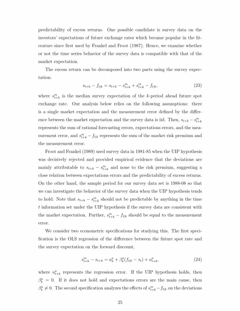
The excess return can be decomposed into two parts using the survey expec-

tation:

st+k − ft|k = st+k − smt+k + smt+k − ft|k, (23)

where smt+k is the median survey expectation of the k-period ahead future spot

exchange rate. Our analysis below relies on the following assumptions: there

is a single market expectation and the measurement error defined by the differ-

ence between the market expectation and the survey data is iid. Then, st+k − smt+k

represents the sum of rational forecasting errors, expectations errors, and the mea-

surement error, and smt+k−ft|k represents the sum of the market risk premium and

the measurement error.

Froot and Frankel (1989) used survey data in 1981-85 when the UIP hypothesis

was decisively rejected and provided empirical evidence that the deviations are

mainly attributable to st+k − smt+k and none to the risk premium, suggesting a

close relation between expectations errors and the predictability of excess returns.

On the other hand, the sample period for our survey data set is 1988-08 so that

we can investigate the behavior of the survey data when the UIP hypothesis tends

to hold. Note that st+k − smt+k should not be predictable by anything in the time

t information set under the UIP hypothesis if the survey data are consistent with

the market expectation. Further, smt+k − ft|k should be equal to the measurement

error.

We consider two econometric specifications for studying this. The first speci-

fication is the OLS regression of the difference between the future spot rate and

the survey expectation on the forward discount,

smt+k − st+k = aak + βak(ft|k − st) + uat+k, (24)

where uat+k represents the regression error. If the UIP hypothesis holds, then

βak = 0. If it does not hold and expectations errors are the main cause, then

βak ̸= 0. The second specification analyzes the effects of smt+k−ft|k on the deviations

25

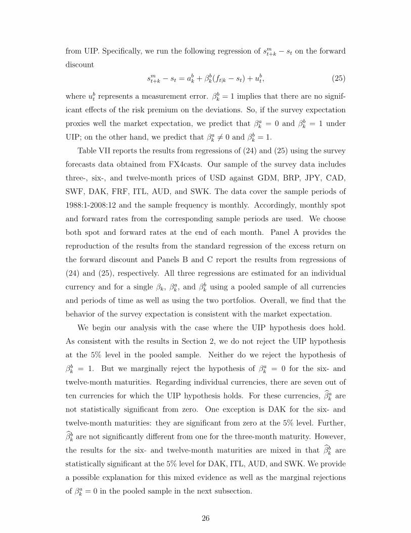
from UIP. Specifically, we run the following regression of smt+k − st on the forward

discount

smt+k − st = abk + βbk(ft|k − st) + ubt , (25)

where ubt represents a measurement error. βbk = 1 implies that there are no signif-

icant effects of the risk premium on the deviations. So, if the survey expectation

proxies well the market expectation, we predict that βak = 0 and βb

k = 1 under

UIP; on the other hand, we predict that βak ̸= 0 and βb

k = 1.

Table VII reports the results from regressions of (24) and (25) using the survey

forecasts data obtained from FX4casts. Our sample of the survey data includes

three-, six-, and twelve-month prices of USD against GDM, BRP, JPY, CAD,

SWF, DAK, FRF, ITL, AUD, and SWK. The data cover the sample periods of

1988:1-2008:12 and the sample frequency is monthly. Accordingly, monthly spot

and forward rates from the corresponding sample periods are used. We choose

both spot and forward rates at the end of each month. Panel A provides the

reproduction of the results from the standard regression of the excess return on

the forward discount and Panels B and C report the results from regressions of

(24) and (25), respectively. All three regressions are estimated for an individual

currency and for a single βk, βak , and βb

k using a pooled sample of all currencies

and periods of time as well as using the two portfolios. Overall, we find that the

behavior of the survey expectation is consistent with the market expectation.

We begin our analysis with the case where the UIP hypothesis does hold.

As consistent with the results in Section 2, we do not reject the UIP hypothesis

at the 5% level in the pooled sample. Neither do we reject the hypothesis of

βbk = 1. But we marginally reject the hypothesis of βa

k = 0 for the six- and

twelve-month maturities. Regarding individual currencies, there are seven out of

ten currencies for which the UIP hypothesis holds. For these currencies, β̂ak are

not statistically significant from zero. One exception is DAK for the six- and

twelve-month maturities: they are significant from zero at the 5% level. Further,

β̂bk are not significantly different from one for the three-month maturity. However,

the results for the six- and twelve-month maturities are mixed in that β̂bk are

statistically significant at the 5% level for DAK, ITL, AUD, and SWK. We provide

a possible explanation for this mixed evidence as well as the marginal rejections

of βak = 0 in the pooled sample in the next subsection.

26

We now discuss the case where the UIP hypothesis does not hold. The UIP

hypothesis is marginally rejected at the 5% level for both portfolios except for

the turnover-weighted average of one-month excess returns. Regarding individ-

ual currencies, the rejections occur only for four currencies.28 It occurs for JPY

and SWF for all maturities, for the CAD for the three-month, and for GDM for

the six-month and one-year. For these portfolios and individual currencies, β̂ak is

significantly different from zero. An exception is the JPY for the three-month

maturity. On the other hand, β̂bk is statistically indistinguishable from one for all

maturities. Exceptions are JPY for the three-month maturity and GDM for the

six-month maturity.29

We summarize the results from the two cases above (both where the UIP

hypothesis holds and where it does not hold): (i) in general, we do not reject

the hypothesis of βbk = 1 in both cases, consistent with the findings by Froot

and Frankel as well as with ours on the serial dependence of excess returns in the

previous section; (ii) in the case where the UIP hypothesis does not hold, we reject

the hypothesis of βak = 0 consistent again with previous evidence; (iii) smt+k − st+k

is not predictable using the forward discount when the UIP hypothesis holds; (iv)

the results in (i)-(iii) suggest that the survey expectation behaves consistently with

the market expectation defined in equation (17).

5.4 Measurement Error

The key assumption made in regressions (24) and (25) is that measurement

error is iid. To investigate the validity of this assumption, we discuss several sources

of measurement error that may generate a systematic bias in the regressions and

attempt to quantify the magnitude of the bias. First, the survey data were not

collected at the same moment as the contemporaneous spot rate was recorded. To

see how severely this mismatch affects our results, we conduct the same regressions

28Compared to the results from the previous sections, there is a small discrepancy regardingthe rejections of the UIP hypothesis. This may be due to using different sample periods and/ordifferent sample frequency. Nevertheless, we confirm that the deviations from UIP becomesignificantly weakened after 1980s.

29Our results are consistent with Bacchetta, Mertens, and Wincoop (2008) who also usedthe same data between August 1986 and July 2005: they found a strong relation between therejections of the UIP hypothesis and the expectations errors. One apparent difference is thatthe rejections against the UIP hypothesis in their sample appear somewhat stronger than ours.One reason may be the use of different sample period. In particular, their sample includes partof observations from the period of 1980-87 in which the strongest rejections are occurred.

27

(24)-(25) by changing the date of selecting forward and spot exchange rates from

Monday to Friday of the last week of each month.30 The results across different

selection dates are broadly consistent.31 Similarly, Bekaert and Hodrick (1993)

showed that their findings were not much affected by measurement error due to

the failure of taking correctly into account of the delivery structure of the forward

contract. One reason for this insensitivity may be related to the strong persistence

in the forward discount.

Second, the survey data used in the present paper were constructed from a

sample of market participants. Hence, there may exist measurement error if the

sample does not capture the opinions of all participants in the market. However,

this may not be large enough to overturn the above results since the sample con-

sists of large numbers of wealthy investors and financial institutions who actively

participate in the market according to FX4casts. Further, many studies consis-

tently find evidence on the relation between expectation errors and excess returns

using survey data in various financial markets and over different sample periods,

suggesting that our results may not be entirely attributable to a sample selection

bias [see, e.g., Froot and Frankel (1989), Bacchetta, Mertens, and Wincoop (2008),

and references therein].

In addition, there may exist other sources of measurement error which we

have not been able to take into account. Therefore, our objective below is to

identify a systematic pattern between measurement error and the predictor in the

regressions without providing any further explanation for the existence of those

sources. Suppose that the UIP hypothesis holds. Then, the difference between

the estimate and the true value in regressions (24)-(25) can be interpreted as an

estimation error if there are no biases. However, if there were a systematic relation

between measurement error and the predictor for some reasons, this would generate

either a negative or positive bias in the regressions and thus we would consistently

observe a tendency of either downward or upward biases of both β̂ak and β̂b

k. Since

the UIP hypothesis tends to hold for many currencies in our sample during 1988-

08, we use those regressions to identify the direction of the bias. That is, if there

is a positive bias, then we should consistently observe β̂ak > 0 and β̂b

k > 1 under

30According to FX4casts, the survey was e-mailed on the last Friday of the month. Most ofthe forecasts come in on Monday of that week and about 10% on Tuesday. About 10% come inthe previous Friday.

31See the technical and empirical appendix.

28

the UIP hypothesis; otherwise, we should observe β̂ak < 0 and β̂b

k < 1 if there is a

negative bias.

We find a symptom of a positive bias in those regressions. For all the currencies

and maturities for which the UIP hypothesis holds, we find that β̂bk > 1. On the

other hand, β̂ak > 0 for most cases although they are not statistically significant.

These results suggest that there may exist a positive bias. We now attempt to

informally estimate to which extent the magnitude of this bias might affect our

conclusions. Under the assumption of zero estimation errors on average, we cal-

culate the average of the difference between β̂bk and the true value, finding that it

is about 0.6. None of them become statistically significant at the 5% level under

the UIP hypothesis after the correction of this bias by subtracting the average

from both β̂bk and β̂a

k . This may explain the mixed evidence for β̂bk above. We did

the same correction for the case where there are deviations from UIP. However,

this does not overturn the significant relation between the expectation error and

the forward discount, although the evidence appears somewhat weaker. In sum,

we find that measurement error cannot entirely drive our findings, although the

positive bias may affect the results on regressions (24)-(25).

6 Conclusions

This paper investigates the predictability of excess returns in foreign exchange

markets. We first find that both the statistically significant positive serial depen-

dence of foreign excess returns in the entire sample and the very weak (mostly

insignificant) positive serial dependence in Subsample E are consistent with the

predictions of the expectations errors explanation. Our analysis also explains why

previous studies have consistently documented strong predictability of excess re-

turns: the effects of a particular sample period are masked. We, then, link this

new evidence with the changes in forecasting techniques in foreign exchange mar-

kets in the 1980s. Finally, we show that the behavior of the survey expectation

is compatible with the market expectation over both subsample periods. That is,

the difference between the survey expectation and the future exchange rate is not

predictable when the UIP hypothesis holds but the expectations errors are closely

related to the predictability of excess returns when the UIP hypothesis does not

hold. Overall, we find that the expectations errors explanation is consistent with

29

the behavior of excess returns over the entire sample period.

Our results appear robust to the selection of the subsample period, choice of

predictors, and the presence of highly persistent regressors. We show that the very

strong predictability only appears in the 1980s based on the parameter stability

test using rolling samples. Further, we obtain very similar results on the pre-

dictability of excess returns either using past returns through the variance ratio

test or using the forward discount through the typical regression test. Further-

more, the results from the conditional test by Jasson and Moreira confirm that a

statistical phenomenon cannot be the main cause of our findings.

Our new empirical findings on the predictability of excess returns against the

USD deserve further attentions. The first concern is related to the dynamic be-

havior of exchange rates in response to monetary policy shocks. An example is the

delayed overshooting phenomenon, first documented by Eichenbaum and Evans

(1995), which states the dynamic response of currency depreciation (or excess re-

turns) in response to the change in the interest rate difference between the two

countries. We leave as future study for investigating if this phenomenon is also

significantly affected by the influential subsample period. The second concern is

related to the potential effects of peso problems on the deviations from UIP in

1980-87.32 Although peso problems can be a natural candidate for explaining the

new empirical evidence, we also leave this possibility as future study.

32For example, several studies such as Engel and Hamilton (1990), Kaminsky (1993), andEvans and Lewis (1995) related the large swings of the US dollar exchange rates in this timeperiod to peso problems.

30

Appendix A: The Parameter Stability Test

We describe the computation of bootstrap estimates of the uniform test bands

for the stability test under the null of parameter stability βk(j) = 0 for all subsam-

ple j. The justification of this procedure is straightforward under the assumptions

that the regressor is stationary and the error term is iid in equation (1). The

procedure follows.

1. Run 8-year rolling regressions based on (1) and obtain residuals only for the

last one-year observations in each rolling regression.

2. Obtain a bootstrap resample of these residuals using the block bootstrap

method with block size of k.

3. Construct the bootstrap dependent variable using regression (1) with resam-

pled residuals from step 2, the original regressors, and the true parameter

values under the null of parameter stability.

4. Run 8-year rolling regressions on the resampled data from step 3 and store

the estimated slope coefficients as well as the corresponding t-statistics. Then

obtain the minimum and maximum of these sequences of the estimated re-

gression coefficients and the corresponding t-statistics for this resample.

5. Repeat steps 2-4 n times [In the present paper, we set n=10,000.].

6. Calculate 5 and 95 % quantiles from the simulated bootstrap empirical dis-

tribution of the minimum and maximum of the estimated rolling regression

slope parameters as well as the t-statistics.

Appendix B. The Rank-based Median Variance Ratio Test

We briefly describe the procedure of the rank-based median variance ratio test

conducted in Section 4. To take into account the presence of moving average

components in excess returns due to using finer sampling frequency, we divide the

entire sample S = {re1, re2, . . . , reT} into k subsamples in the following way: Sj =

{rej , rek+j, . . . , reT−k+j}, for j = 1, · · · , k. Let the sample variance ratio, V̂ Rj(q), for

31

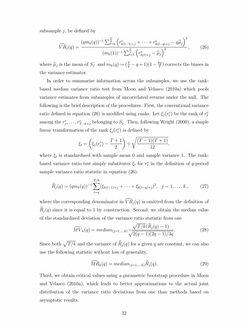
subsample j, be defined by

V̂ Rj(q) =(qmk(q))

−1∑T

kt=q

(rek(t−1)+j + · · ·+ rek(t−q)+j − qµ̂j

)2

(mk(1))−1∑T

kt=1

(rek(t)+j − µ̂j

)2 , (26)

where µ̂j is the mean of Sj and mk(q) = (Tk− q+1)(1− kq

T) corrects the biases in

the variance estimator.

In order to summarize information across the subsamples, we use the rank-

based median variance ratio test from Moon and Velasco (2010a) which pools

variance estimates from subsamples of uncorrelated returns under the null. The

following is the brief description of the procedures. First, the conventional variance

ratio defined in equation (26) is modified using ranks. Let ξj(ret ) be the rank of ret

among the rej , . . . , reT−k+j belonging to Sj. Then, following Wright (2000), a simple

linear transformation of the rank ξj(ret ) is defined by

ξt =

(ξj(r

et )−

T + 1

2

)÷

√(T − 1)(T + 1)

12,

where ξt is standardized with sample mean 0 and sample variance 1. The rank-

based variance ratio test simply substitutes ξt for ret in the definition of q-period

sample variance ratio statistic in equation (26):

R̂j(q) = (qmk(q))−1

T/k∑t=q

(ξk(t−1)+j + · · ·+ ξk(t−q)+j)2, j = 1, . . . , k., (27)

where the corresponding denominator in V̂ Rj(q) is omitted from the definition of

R̂j(q) since it is equal to 1 by construction. Second, we obtain the median value

of the standardized deviation of the variance ratio statistic from one

M̂V k(q) = median(j=1,...,k)

√T/k(R̂j(q)− 1)√

2(q − 1)(2q − 1)/3q. (28)

Since both√T/k and the variance of R̂j(q) for a given q are constant, we can also

use the following statistic without loss of generality,

M̂Rk(q) = median(j=1,...,k)R̂j(q). (29)

Third, we obtain critical values using a parametric bootstrap procedure in Moon

and Velasco (2010a), which leads to better approximations to the actual joint

distribution of the variance ratio deviations from one than methods based on

asymptotic results.

32

References

Alvarez, Fernando, Andrew Atkeson, and Patrick J. Kehoe, 2009, Time-Varying Risk,Interest Rates, and Exchange Rates in General Equilibrium, Review of EconomicStudies 76 (3), 851-878.

Abel, Andrew B, 1988, Stock Prices under Time-Varying Dividend Risk : An ExactSolution in an Infinite-Horizon General Equilibrium Model, Journal of MonetaryEconomics Volume 22 (3), 375-393.

Baillie, Richard T., and Tim Bollerslev, 2000, The Forward Discount Anomaly Is NotAs Bad As You Think, Journal of International Money and Finance 19, 471-488.

Bacchetta, Philippe, Elmar Mertens, and Eric van Wincoop, 2008, Predictability in Fi-nancial Markets: What Do Survey Expectations Tell Us?, Journal of InternationalMoney and Finance 28, 406-26.

Bacchetta, Philippe, and Eric van Wincoop, 2010, Infrequent Portfolio Decisions: ASolution to the Forward Discount Puzzle, American Economic Review 100, 837-869.

Backus, David K., Silverio Foresi, and Chris I. Telmer, 2001, Affine Term StructureModels and the Forward Premium Anomaly, Journal of Finance 56 (1), 279-304.

Bansal, Ravi, 1997, An Exploration of the Forward Discount Puzzle in Currency Mar-kets, The Review of Financial Studies 10, 369-403.

Bekaert, Geert, and Robert J. Hodrick, 1992, Characterizing Predictable Componentsin Excess Returns on Equity and Foreign Exchange Markets, Journal of Finance47, 467-509.

Bekaert, Geert, and Robert J. Hodrick, 1993, On Biases in the Measurement of ForeignExchange Risk Premiums, Journal of International Money and Finance 12(2),115-38.

Campbell, John Y. and N. Gregory Mankiw, 1987, Are Output Fluctuations Transi-tory?, Quarterly Journal of Economics, 102 (4), 857-880

Campbell, John Y. and Motohiro Yogo, 2006, Efficient Tests of Stock Return Pre-dictability, Journal of Financial Economics 81(1), 27-60.

Campbell, John Y, 1991, A Variance Decomposition for Stock Returns, Economic Jour-nal 101, 157-179.

Chinn, Menzie D., 2006, The (Partial) Rehabilitation of Interest Rate Parity in theFloating Rate Era: Longer Horizons, Alternative Expectations, and EmergingMarkets, Journal of International Money and Finance 26, 7-21.

Cochrane, John H., 1988, How Big Is the Random Walk in GNP?, The Journal ofPolitical Economy 96 (5), 893-920.

De Long, J. Bradford, Andrei Shleifer, Lawrence H. Summers, and Robert J. Wald-mann, 1990a, Noise Trader Risk in Financial Markets, Journal of Political Econ-omy 98 (4), 703-738

33

De Long, J. Bradford, Andrei Shleifer, Lawrence H. Summers, and Robert J. Wald-mann, 1990b, Positive Feedback Investment Strategies and Destabilizing RationalSpeculation, Journal of Finance 45, 375-395.

Dornbusch, Rudiger, 1976, Expectations and Exchange Rate Dynamics, Journal ofPolitical Economy 84, 1161-76.

Eichenbaum, Martin, and Charles L. Evans, 1995, Some Empirical Evidence on theEffects of Shocks to Monetary Policy on Exchange Rates, The Quarterly Journalof Economics 110 (4), 975-1009.

Engel, Charles, 1996, The Forward Discount Anomaly and the Risk Premium: A Surveyof Recent Evidence, Journal of Empirical Finance 3, 123-192.

Engel, Charles, and James D. Hamilton, 1990, Long Swings in the Dollar: Are They inthe Data and Do Markets Know It, The American Economic Review 80, 689-713.

Engel, Charles, and Kenneth D. West, 2005, Exchange Rates and Fundamentals, Jour-nal of Political Economy, 113, (2005) 485-517.

Evans, Martin D. D., and Karen K. Lewis 1995, Do long-term Swings in the DollarAffect Estimates of the Risk Premia?, Review of Financial Studies 8 (3), 709-742.

Evans, GeorgeW., 1986, A Test for Speculative Bubbles in the Sterling-Dollar ExchangeRate: 1981-84, The American Economic Review 76(4), 621-636.

Fama, Eugene F., and Kenneth R. French, 1988, Permanent and Temporary Compo-nents of Stock Prices, Journal of Political Economy 96, 246-273.

Fama, Eugene F., 1984, Forward and Spot Exchange Rates? Journal of MonetaryEconomics 14, 319-338.

Flood, Robert P. and Andrew K. Rose, 2002, Uncovered Interest Parity in Crisis: TheInterest Rate Defense in the 1990s, IMF Staff Papers.

Frankel, Jeffrey A., and Kenneth A. Froot, 1987, Using Survey Data to Test StandardPropositions Regarding Exchange Rate Expectations, American Economic Review77, 393-407.

Frankel, Jeffrey A., and Kenneth A. Froot, 1990a, Chartists, Fundamentalists, andTrading in the Foreign Exchange Market, American Economic Review (Papersand Proceedings) 80, 181-185.

Frankel, Jeffrey A., and Kenneth A. Froot; 1990b, Chartists, Fundamentalists, andDemand for Dollars, In Anthony S. Courakis and Mark P. Taylor, ed.: PrivateBehavior and Interdependent Government Policy (Clarendon Press, Oxford).

Froot, Kenneth A., and Jeffrey A. Frankel, 1989, Forward Discount Bias: Is it anExchange Risk Premium?, Quarterly Journal of Economics 104, 139-161.

Gourinchas, Pierre-Olivier, and Aaron Tornell, 2004, Exchange Rate Puzzles and Dis-torted Beliefs, Journal of International Economics 64(2), 303-333.

Hodrick, Robert J., 1989, Risk, Uncertainty, and Exchange Rates, Journal of MonetaryEconomics 23(3): 433-59.

34

Jansson, Michael and Marcelo J. Moreira, 2006, Optimal Inference in Regression Modelswith Nearly Integrated Regressors, Econometrica 74(3), 681-714.

Kaminsky, Graciela L. 1993, Is There a Peso Problem? Evidence from the Dollar/PoundExchange Rate, 1976-1987, The American Economic Review, 83 (3), 450-472.

Krugman, Paul R. 1985, Is the strong dollar sustainable?, Proceedings, Federal ReserveBank of Kansas City, 103-155.

Lewis, Karen K.; 1995, Puzzles in International Financial Markets, in Gene Grossmanand Kenneth Rogoff, ed.: Handbook of International Economics, vol 3 (NorthHolland, Amsterdam)

Liu, Christina Y., and Jia He, 1991, A Variance-Ratio Test of RandomWalks in ForeignExchange Rates, The Journal of Finance 46(2), 773-785.

Lo, Andrew W., and A. Craig McKinlay, 1988, Stock Market Prices Do Not FollowRandom Walks: Evidence from a Simple Specification Test, Review of FinancialStudies 1, 41-66.

Lo, Andrew W., and A. Craig McKinlay, 1989, The Size and Power of the VarianceRatio Tests in Finite Samples: A Monte Carlo Investigation, Journal of Econo-metrics, 40, 203-38.

Mark, Nelson C., and Yangru Wu, 1998, Rethinking Deviations from Uncovered InterestParity: The Role of Covariance Risk and Noise, Economic Journal 108 (451), 1686-06

Mankiw, N. Gregory and Matthew D. Shapiro, 1986, Do We Reject Too Often? SmallSample Properties of Tests of Rational Expectations Models, Economics Letters20, 139-145.

Maynard, Alex and Peter C. B. Phillips 2001, Rethinking an Old Empirical Puzzle:Econometric Evidence on the Forward Discount Anomaly, Journal of AppliedEconometrics 16(6), 671-708.

Maynard, Alex, 2006, The Forward Discount Anomaly: Statistical Artifact or EconomicPuzzle? New evidence from Robust Tests, Canadian Journal of Economics 39 (4),1244-1281.

Meese, Richard A., 1986, Testing for Bubbles in Exchange Markets: A Case of SparklingRates?, The Journal of Political Economy (94), 345-373.

Moon, Seongman, and Carlos Velasco, 2010a, Predictability Tests for the ExpectationsHypothesis in the Presence of MA Disturbances, mimeo, Universidad Carlos IIIde Madrid.

Moon, Seongman, and Carlos Velasco, 2010b, On the Properties of Regression Tests ofAsset Return Predictability, mimeo, Universidad Carlos III de Madrid.

Newey, Whitney, and Kenneth West, 1987, A Simple, Positive Semi-Definite, Het-eroscedastic and Autocorrelation Consistent Covariance Matrix, Econometrica 55,703-708.

35

Obstfeld, Maurice and Kenneth Rogoff, 2002, Risk and Exchange Rates, in ElhananHelpman and Effraim Sadka (eds.), Contemporary Economic Policy: Essays inHonor of Assaf Razin. Cambridge: Cambridge University Press.

Polk Christopher, Samuel Thompson, and Tuomo Vuolteenaho, 2006, Cross-SectionalForecasts of the Equity Premium, Journal of Financial Economics 81 (1), 101-141.

Poterba, James M., and Lawrence H. Summers, 1988, Mean Reversion in Stock Prices:Evidence and Implications, Journal of Financial Economics 22, 27-59.

Stambaugh, Robert F., 1999, Predictive Regressions, Journal of Financial Economics54, 375-421.

Verdelhan, Adrien, 2010, A Habit-Based Explanation of the Exchange Rate Risk Pre-mium, Journal of Finance 65, 123-145.

West, Kenneth 2008, Econometric Analysis of Present Value Models when the DiscountFactor is Near One, mimeo, University of Wisconsin.

Wright, Jonathan H., 2000, Alternative Variance Ratio Tests Using Ranks and Signs,Journal of Business and Economic Statistics 18, 1-9.

36

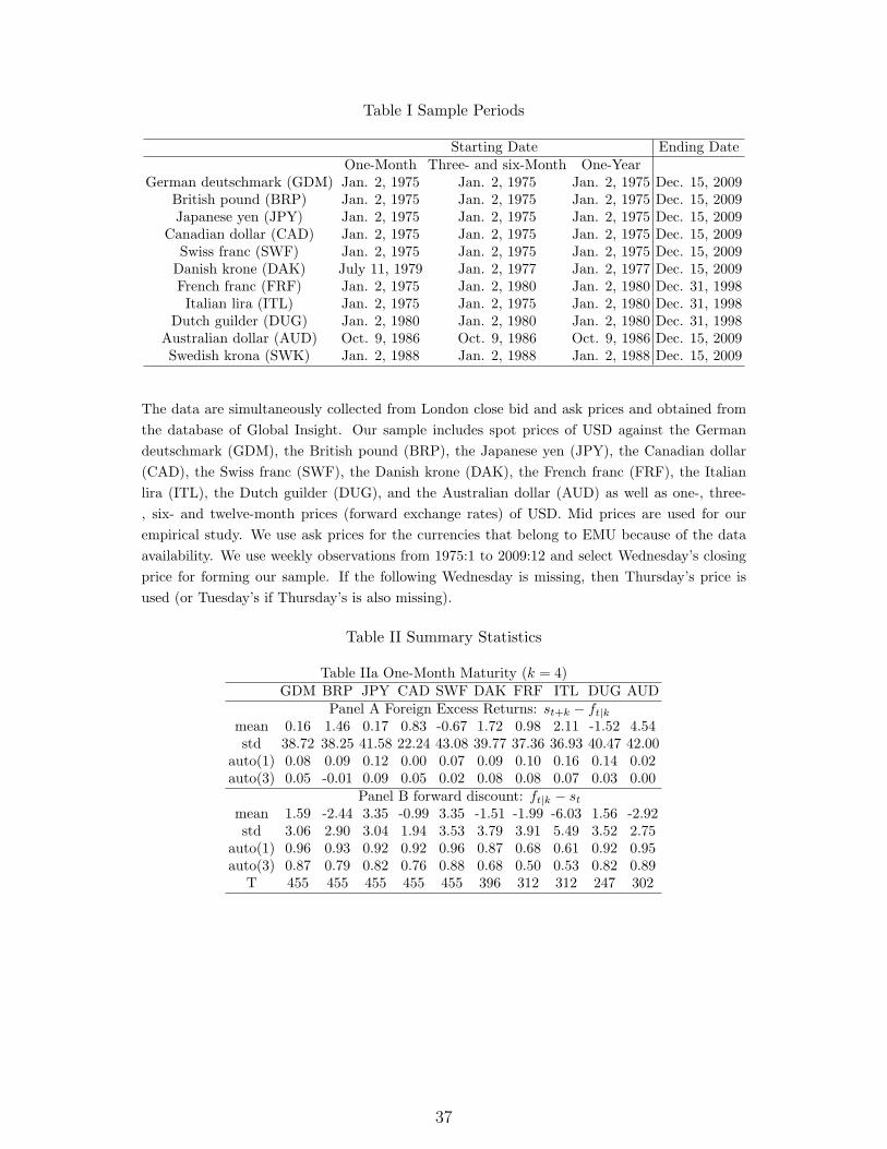
Table I Sample Periods

Starting Date Ending DateOne-Month Three- and six-Month One-Year

German deutschmark (GDM) Jan. 2, 1975 Jan. 2, 1975 Jan. 2, 1975 Dec. 15, 2009British pound (BRP) Jan. 2, 1975 Jan. 2, 1975 Jan. 2, 1975 Dec. 15, 2009Japanese yen (JPY) Jan. 2, 1975 Jan. 2, 1975 Jan. 2, 1975 Dec. 15, 2009

Canadian dollar (CAD) Jan. 2, 1975 Jan. 2, 1975 Jan. 2, 1975 Dec. 15, 2009Swiss franc (SWF) Jan. 2, 1975 Jan. 2, 1975 Jan. 2, 1975 Dec. 15, 2009Danish krone (DAK) July 11, 1979 Jan. 2, 1977 Jan. 2, 1977 Dec. 15, 2009French franc (FRF) Jan. 2, 1975 Jan. 2, 1980 Jan. 2, 1980 Dec. 31, 1998Italian lira (ITL) Jan. 2, 1975 Jan. 2, 1975 Jan. 2, 1980 Dec. 31, 1998

Dutch guilder (DUG) Jan. 2, 1980 Jan. 2, 1980 Jan. 2, 1980 Dec. 31, 1998Australian dollar (AUD) Oct. 9, 1986 Oct. 9, 1986 Oct. 9, 1986 Dec. 15, 2009Swedish krona (SWK) Jan. 2, 1988 Jan. 2, 1988 Jan. 2, 1988 Dec. 15, 2009

The data are simultaneously collected from London close bid and ask prices and obtained from

the database of Global Insight. Our sample includes spot prices of USD against the German

deutschmark (GDM), the British pound (BRP), the Japanese yen (JPY), the Canadian dollar

(CAD), the Swiss franc (SWF), the Danish krone (DAK), the French franc (FRF), the Italian

lira (ITL), the Dutch guilder (DUG), and the Australian dollar (AUD) as well as one-, three-

, six- and twelve-month prices (forward exchange rates) of USD. Mid prices are used for our

empirical study. We use ask prices for the currencies that belong to EMU because of the data

availability. We use weekly observations from 1975:1 to 2009:12 and select Wednesday’s closing

price for forming our sample. If the following Wednesday is missing, then Thursday’s price is

used (or Tuesday’s if Thursday’s is also missing).

Table II Summary Statistics

Table IIa One-Month Maturity (k = 4)GDM BRP JPY CAD SWF DAK FRF ITL DUG AUD

Panel A Foreign Excess Returns: st+k − ft|kmean 0.16 1.46 0.17 0.83 -0.67 1.72 0.98 2.11 -1.52 4.54std 38.72 38.25 41.58 22.24 43.08 39.77 37.36 36.93 40.47 42.00

auto(1) 0.08 0.09 0.12 0.00 0.07 0.09 0.10 0.16 0.14 0.02auto(3) 0.05 -0.01 0.09 0.05 0.02 0.08 0.08 0.07 0.03 0.00

Panel B forward discount: ft|k − stmean 1.59 -2.44 3.35 -0.99 3.35 -1.51 -1.99 -6.03 1.56 -2.92std 3.06 2.90 3.04 1.94 3.53 3.79 3.91 5.49 3.52 2.75

auto(1) 0.96 0.93 0.92 0.92 0.96 0.87 0.68 0.61 0.92 0.95auto(3) 0.87 0.79 0.82 0.76 0.88 0.68 0.50 0.53 0.82 0.89

T 455 455 455 455 455 396 312 312 247 302

37

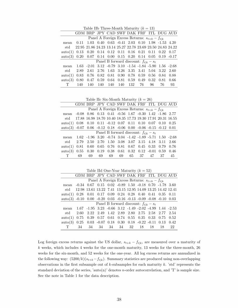
Table IIb Three-Month Maturity (k = 13)GDM BRP JPY CAD SWF DAK FRF ITL DUG AUD

Panel A Foreign Excess Returns: st+k − ft|kmean 0.11 1.03 0.40 0.63 -0.41 2.03 0.10 1.98 -1.53 4.20std 22.95 21.86 24.23 13.14 25.27 22.78 23.69 23.50 24.83 24.22

auto(1) 0.13 0.20 0.14 0.12 0.11 0.16 0.21 0.11 0.22 0.17auto(3) 0.20 0.07 0.14 0.00 0.15 0.20 0.14 0.05 0.19 -0.17

Panel B forward discount: ft|k − stmean 1.63 -2.01 3.12 -0.79 3.10 -1.54 -1.84 -5.90 1.56 -2.68std 2.89 2.61 2.76 1.63 3.26 3.35 3.41 5.04 3.22 2.60

auto(1) 0.83 0.76 0.82 0.81 0.90 0.78 0.59 0.56 0.84 0.88auto(3) 0.80 0.47 0.59 0.64 0.81 0.59 0.49 0.32 0.81 0.66

T 140 140 140 140 140 132 76 96 76 93

Table IIc Six-Month Maturity (k = 26)GDM BRP JPY CAD SWF DAK FRF ITL DUG AUD

Panel A Foreign Excess Returns: st+k − ft|kmean -0.08 0.86 0.13 0.41 -0.56 1.67 -0.30 1.42 -1.86 2.77std 17.88 16.98 18.70 10.40 18.35 17.73 19.30 17.91 20.31 16.55

auto(1) 0.08 0.10 0.11 -0.12 0.07 0.11 0.10 0.07 0.10 0.25auto(3) -0.07 0.06 -0.12 0.18 -0.06 0.00 -0.06 -0.15 -0.12 0.01

Panel B forward discount: ft|k − stmean 1.62 -1.96 3.20 -0.74 3.04 -1.42 -1.89 -5.71 1.50 -2.68std 2.79 2.50 2.70 1.50 3.08 3.07 3.15 4.18 3.11 2.66

auto(1) 0.81 0.60 0.65 0.76 0.81 0.67 0.45 0.33 0.79 0.76auto(3) 0.55 0.30 0.19 0.38 0.61 0.32 0.12 -0.01 0.59 0.46

T 69 69 69 69 69 65 37 47 37 45

Table IId One-Year Maturity (k = 52)GDM BRP JPY CAD SWF DAK FRF ITL DUG AUD

Panel A Foreign Excess Returns: st+k − ft|kmean -0.34 0.67 0.15 0.02 -0.89 1.50 -0.18 0.70 -1.78 3.60std 12.98 13.61 13.22 7.41 13.15 12.95 14.09 13.25 14.42 12.41

auto(1) 0.28 0.01 0.17 0.09 0.24 0.28 0.40 0.41 0.35 0.11auto(3) -0.10 0.00 -0.20 0.03 -0.16 -0.13 -0.09 -0.08 -0.10 0.03

Panel B forward discount: ft|k − stmean 1.67 -1.95 3.23 -0.66 3.12 -1.49 -2.02 -4.99 1.44 -2.53std 2.60 2.22 2.49 1.42 2.89 2.80 2.75 2.58 2.77 2.54

auto(1) 0.75 0.39 0.57 0.61 0.74 0.55 0.35 0.33 0.75 0.52auto(3) 0.25 0.03 -0.07 0.18 0.30 0.18 -0.22 -0.11 0.13 0.42

T 34 34 34 34 34 32 18 18 18 22

Log foreign excess returns against the US dollar, st+k − ft|k, are measured over a maturity of

k weeks, which includes 4 weeks for the one-month maturity, 13 weeks for the three-month, 26

weeks for the six-month, and 52 weeks for the one-year. All log excess returns are annualized in

the following way: (5200/k)(st+k−ft|k). Summary statistics are produced using non-overlapping

observations in the first subsample out of k-subsamples for each maturity k. ’std’ represents the

standard deviation of the series, ’auto(n)’ denotes n-order autocorrelation, and ’T’ is sample size.

See the note in Table 1 for the data description.

38

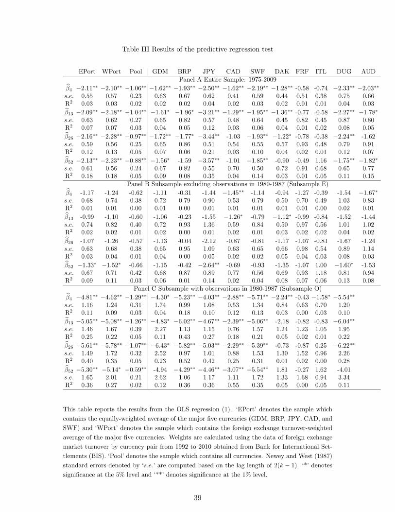
Table III Results of the predictive regression test

EPort WPort Pool GDM BRP JPY CAD SWF DAK FRF ITL DUG AUDPanel A Entire Sample: 1975-2009

β̂4 −2.11∗∗ −2.10∗∗ −1.06∗∗ −1.62∗∗ −1.93∗∗ −2.50∗∗ −1.62∗∗ −2.19∗∗ −1.28∗∗ -0.58 -0.74 −2.33∗∗ −2.03∗∗

s.e. 0.55 0.57 0.23 0.63 0.67 0.62 0.41 0.59 0.44 0.51 0.38 0.75 0.66R2 0.03 0.03 0.02 0.02 0.02 0.04 0.02 0.03 0.02 0.01 0.01 0.04 0.03

β̂13 −2.09∗∗ −2.18∗∗ −1.04∗∗ −1.61∗ −1.96∗ −3.21∗∗ −1.29∗∗ −1.95∗∗ −1.36∗∗ -0.77 -0.58 −2.27∗∗ −1.78∗

s.e. 0.63 0.62 0.27 0.65 0.82 0.57 0.48 0.64 0.45 0.82 0.45 0.87 0.80R2 0.07 0.07 0.03 0.04 0.05 0.12 0.03 0.06 0.04 0.01 0.02 0.08 0.05

β̂26 −2.16∗∗ −2.28∗∗ −0.97∗∗ −1.72∗∗ −1.77∗ −3.44∗∗ -1.03 −1.93∗∗ −1.22∗ -0.78 -0.38 −2.24∗∗ -1.62s.e. 0.59 0.56 0.25 0.65 0.86 0.51 0.54 0.55 0.57 0.93 0.48 0.79 0.91R2 0.12 0.13 0.05 0.07 0.06 0.21 0.03 0.10 0.04 0.02 0.01 0.12 0.07

β̂52 −2.13∗∗ −2.23∗∗ −0.88∗∗ −1.56∗ -1.59 −3.57∗∗ -1.01 −1.85∗∗ -0.90 -0.49 1.16 −1.75∗∗ −1.82∗

s.e. 0.61 0.56 0.24 0.67 0.82 0.55 0.70 0.50 0.72 0.91 0.68 0.65 0.77R2 0.18 0.18 0.05 0.09 0.08 0.35 0.04 0.14 0.03 0.01 0.05 0.11 0.15

Panel B Subsample excluding observations in 1980-1987 (Subsample E)

β̂4 -1.17 -1.24 -0.62 -1.11 -0.31 -1.44 −1.45∗∗ -1.14 -0.94 -1.27 -0.39 -1.54 −1.67∗

s.e. 0.68 0.74 0.38 0.72 0.79 0.90 0.53 0.79 0.50 0.70 0.49 1.03 0.83R2 0.01 0.01 0.00 0.01 0.00 0.01 0.01 0.01 0.01 0.01 0.00 0.02 0.01

β̂13 -0.99 -1.10 -0.60 -1.06 -0.23 -1.55 −1.26∗ -0.79 −1.12∗ -0.99 -0.84 -1.52 -1.44s.e. 0.74 0.82 0.40 0.72 0.93 1.36 0.59 0.84 0.50 0.97 0.56 1.01 1.02R2 0.02 0.02 0.01 0.02 0.00 0.01 0.02 0.01 0.03 0.02 0.02 0.04 0.02

β̂26 -1.07 -1.26 -0.57 -1.13 -0.04 -2.12 -0.87 -0.81 -1.17 -1.07 -0.81 -1.67 -1.24s.e. 0.63 0.68 0.38 0.65 0.95 1.09 0.63 0.65 0.66 0.98 0.54 0.89 1.14R2 0.03 0.04 0.01 0.04 0.00 0.05 0.02 0.02 0.05 0.04 0.03 0.08 0.03

β̂52 −1.33∗ −1.52∗ -0.66 -1.15 -0.42 −2.64∗∗ -0.69 -0.93 -1.35 -1.07 1.00 −1.60∗ -1.53s.e. 0.67 0.71 0.42 0.68 0.87 0.89 0.77 0.56 0.69 0.93 1.18 0.81 0.94R2 0.09 0.11 0.03 0.06 0.01 0.14 0.02 0.04 0.08 0.07 0.06 0.13 0.08

Panel C Subsample with observations in 1980-1987 (Subsample O)

β̂4 −4.81∗∗ −4.62∗∗ −1.29∗∗ −4.30∗ −5.23∗∗ −4.03∗∗ −2.88∗∗ −5.71∗∗ −2.24∗∗ -0.43 −1.58∗ −5.54∗∗

s.e. 1.16 1.24 0.31 1.74 0.99 1.08 0.53 1.34 0.84 0.63 0.70 1.20R2 0.11 0.09 0.03 0.04 0.18 0.10 0.12 0.13 0.03 0.00 0.03 0.10

β̂13 −5.05∗∗ −5.08∗∗ −1.26∗∗ −4.83∗ −6.02∗∗ −4.67∗∗ −2.39∗∗ −5.06∗∗ -2.18 -0.82 -0.83 −6.04∗∗

s.e. 1.46 1.67 0.39 2.27 1.13 1.15 0.76 1.57 1.24 1.23 1.05 1.95R2 0.25 0.22 0.05 0.11 0.43 0.27 0.18 0.21 0.05 0.02 0.01 0.22

β̂26 −5.61∗∗ −5.78∗∗ −1.07∗∗ −6.43∗ −5.82∗∗ −5.03∗∗ −2.29∗∗ −5.39∗∗ -0.73 -0.87 0.25 −6.22∗∗

s.e. 1.49 1.72 0.32 2.52 0.97 1.01 0.88 1.53 1.30 1.52 0.96 2.26R2 0.40 0.35 0.05 0.23 0.52 0.42 0.25 0.31 0.01 0.02 0.00 0.28

β̂52 −5.30∗∗ −5.14∗ −0.59∗∗ -4.94 −4.29∗∗ −4.46∗∗ −3.07∗∗ −5.54∗∗ 1.81 -0.27 1.62 -4.01s.e. 1.65 2.01 0.21 2.62 1.06 1.17 1.11 1.72 1.33 1.68 0.94 3.34R2 0.36 0.27 0.02 0.12 0.36 0.36 0.55 0.35 0.05 0.00 0.05 0.11

This table reports the results from the OLS regression (1). ‘EPort’ denotes the sample which

contains the equally-weighted average of the major five currencies (GDM, BRP, JPY, CAD, and

SWF) and ‘WPort’ denotes the sample which contains the foreign exchange turnover-weighted

average of the major five currencies. Weights are calculated using the data of foreign exchange

market turnover by currency pair from 1992 to 2010 obtained from Bank for International Set-

tlements (BIS). ‘Pool’ denotes the sample which contains all currencies. Newey and West (1987)

standard errors denoted by ‘s.e.’ are computed based on the lag length of 2(k − 1). ‘*’ denotes

significance at the 5% level and ‘**’ denotes significance at the 1% level.

39

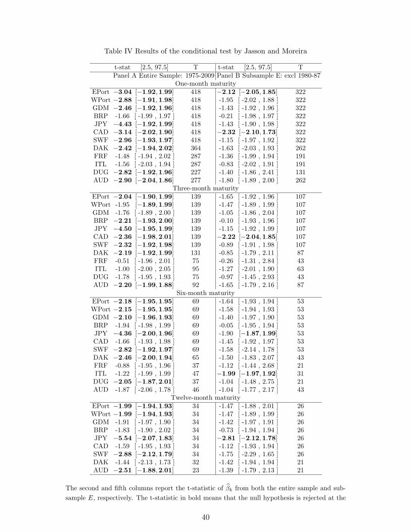
Table IV Results of the conditional test by Jasson and Moreira

t-stat [2.5, 97.5] T t-stat [2.5, 97.5] TPanel A Entire Sample: 1975-2009 Panel B Subsample E: excl 1980-87

One-month maturityEPort −3.04 [−1.92,1.99] 418 −2.12 [−2.05,1.85] 322WPort −2.88 [−1.91,1.98] 418 -1.95 [ -2.02 , 1.88 ] 322GDM −2.46 [−1.92,1.96] 418 -1.43 [ -1.92 , 1.96 ] 322BRP -1.66 [ -1.99 , 1.97 ] 418 -0.21 [ -1.98 , 1.97 ] 322JPY −4.43 [−1.92,1.99] 418 -1.43 [ -1.90 , 1.98 ] 322CAD −3.14 [−2.02,1.90] 418 −2.32 [−2.10,1.73] 322SWF −2.96 [−1.93,1.97] 418 -1.15 [ -1.97 , 1.92 ] 322DAK −2.42 [−1.94,2.02] 364 -1.63 [ -2.03 , 1.93 ] 262FRF -1.48 [ -1.94 , 2.02 ] 287 -1.36 [ -1.99 , 1.94 ] 191ITL -1.56 [ -2.03 , 1.94 ] 287 -0.83 [ -2.02 , 1.91 ] 191DUG −2.82 [−1.92,1.96] 227 -1.40 [ -1.86 , 2.41 ] 131AUD −2.90 [−2.04,1.86] 277 -1.80 [ -1.89 , 2.00 ] 262

Three-month maturityEPort −2.04 [−1.90,1.99] 139 -1.65 [ -1.92 , 1.96 ] 107WPort -1.95 [−1.89,1.99] 139 -1.47 [ -1.89 , 1.99 ] 107GDM -1.76 [ -1.89 , 2.00 ] 139 -1.05 [ -1.86 , 2.04 ] 107BRP −2.21 [−1.93,2.00] 139 -0.10 [ -1.93 , 1.96 ] 107JPY −4.50 [−1.95,1.99] 139 -1.15 [ -1.92 , 1.99 ] 107CAD −2.36 [−1.98,2.01] 139 −2.22 [−2.04,1.85] 107SWF −2.32 [−1.92,1.98] 139 -0.89 [ -1.91 , 1.98 ] 107DAK −2.19 [−1.92,1.99] 131 -0.85 [ -1.79 , 2.11 ] 87FRF -0.51 [ -1.96 , 2.01 ] 75 -0.26 [ -1.31 , 2.84 ] 43ITL -1.00 [ -2.00 , 2.05 ] 95 -1.27 [ -2.01 , 1.90 ] 63DUG -1.78 [ -1.95 , 1.93 ] 75 -0.97 [ -1.45 , 2.93 ] 43AUD −2.20 [−1.99,1.88] 92 -1.65 [ -1.79 , 2.16 ] 87

Six-month maturityEPort −2.18 [−1.95,1.95] 69 -1.64 [ -1.93 , 1.94 ] 53WPort −2.15 [−1.95,1.95] 69 -1.58 [ -1.94 , 1.93 ] 53GDM −2.10 [−1.96,1.93] 69 -1.40 [ -1.97 , 1.90 ] 53BRP -1.94 [ -1.98 , 1.99 ] 69 -0.05 [ -1.95 , 1.94 ] 53JPY −4.36 [−2.00,1.96] 69 -1.90 [−1.87,1.99] 53CAD -1.66 [ -1.93 , 1.98 ] 69 -1.45 [ -1.92 , 1.97 ] 53SWF −2.82 [−1.92,1.97] 69 -1.58 [ -2.14 , 1.78 ] 53DAK −2.46 [−2.00,1.94] 65 -1.50 [ -1.83 , 2.07 ] 43FRF -0.88 [ -1.95 , 1.96 ] 37 -1.12 [ -1.44 , 2.68 ] 21ITL -1.22 [ -1.99 , 1.99 ] 47 −1.99 [−1.97,1.92] 31DUG −2.05 [−1.87,2.01] 37 -1.04 [ -1.48 , 2.75 ] 21AUD -1.87 [ -2.06 , 1.78 ] 46 -1.04 [ -1.77 , 2.17 ] 43

Twelve-month maturityEPort −1.99 [−1.94,1.93] 34 -1.47 [ -1.88 , 2.01 ] 26WPort −1.99 [−1.94,1.93] 34 -1.47 [ -1.89 , 1.99 ] 26GDM -1.91 [ -1.97 , 1.90 ] 34 -1.42 [ -1.97 , 1.91 ] 26BRP -1.83 [ -1.90 , 2.02 ] 34 -0.73 [ -1.94 , 1.94 ] 26JPY −5.54 [−2.07,1.83] 34 −2.81 [−2.12,1.78] 26CAD -1.59 [ -1.95 , 1.93 ] 34 -1.12 [ -1.93 , 1.94 ] 26SWF −2.88 [−2.12,1.79] 34 -1.75 [ -2.29 , 1.65 ] 26DAK -1.44 [ -2.13 , 1.73 ] 32 -1.42 [ -1.94 , 1.94 ] 21AUD −2.51 [−1.88,2.01] 23 -1.39 [ -1.79 , 2.13 ] 21

The second and fifth columns report the t-statistic of β̂k from both the entire sample and sub-

sample E, respectively. The t-statistic in bold means that the null hypothesis is rejected at the

40

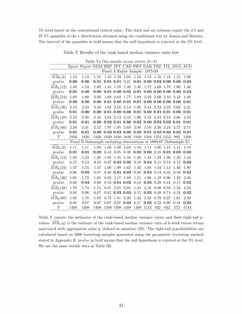
5% level based on the conventional critical value. The third and six columns report the 2.5 and

97.5% quantiles of the t distribution obtained using the conditional test by Jasson and Moreira.

The interval of the quantiles in bold means that the null hypothesis is rejected at the 5% level.

Table V Results of the rank-based median variance ratio test

Table Va One-month excess return (k=4)Eport Wport GDM BRP JPY CAD SWF DAK FRF ITL DUG AUD

Panel A Entire Sample: 1975-09

M̂Rk(2) 1.13 1.13 1.10 1.10 1.10 1.04 1.10 1.13 1.10 1.18 1.15 1.09pvalue 0.00 0.00 0.01 0.01 0.01 0.21 0.01 0.00 0.02 0.00 0.00 0.03

M̂Rk(12) 1.49 1.54 1.60 1.45 1.59 1.40 1.48 1.72 1.69 1.78 1.90 1.46pvalue 0.01 0.00 0.00 0.01 0.00 0.02 0.01 0.00 0.00 0.00 0.00 0.03

M̂Rk(24) 1.89 1.99 2.09 1.69 2.04 1.77 1.80 2.23 2.09 2.10 2.42 1.92pvalue 0.00 0.00 0.00 0.01 0.00 0.01 0.01 0.00 0.00 0.00 0.00 0.01

M̂Rk(36) 2.13 2.24 2.34 1.92 2.16 2.14 1.98 2.44 2.23 2.23 2.62 2.21pvalue 0.01 0.00 0.00 0.01 0.00 0.00 0.01 0.00 0.01 0.01 0.00 0.01

M̂Rk(48) 2.23 2.30 2.42 2.04 2.13 2.43 1.96 2.53 2.24 2.18 2.66 2.52pvalue 0.01 0.01 0.00 0.02 0.01 0.00 0.02 0.00 0.02 0.02 0.01 0.01

M̂Rk(60) 2.29 2.31 2.52 1.97 1.95 2.69 2.00 2.59 2.30 2.24 2.77 2.71pvalue 0.01 0.01 0.00 0.03 0.03 0.00 0.03 0.01 0.03 0.03 0.02 0.01

T 1820 1820 1820 1820 1820 1820 1820 1584 1252 1252 992 1208Panel B Subsample excluding observations in 1980-87 (Subsample E)

M̂Rk(2) 1.11 1.11 1.09 1.06 1.08 1.03 1.10 1.14 1.06 1.15 1.14 1.10pvalue 0.01 0.01 0.02 0.10 0.05 0.30 0.02 0.00 0.18 0.01 0.03 0.03

M̂Rk(12) 1.20 1.23 1.26 1.05 1.45 1.34 1.28 1.43 1.33 1.30 1.33 1.42pvalue 0.17 0.13 0.10 0.37 0.02 0.05 0.10 0.04 0.11 0.13 0.15 0.03

M̂Rk(24) 1.47 1.55 1.47 1.00 1.99 1.62 1.43 1.69 1.44 1.12 1.46 1.80pvalue 0.08 0.05 0.07 0.46 0.01 0.03 0.08 0.04 0.13 0.32 0.16 0.02

M̂Rk(36) 1.65 1.73 1.65 0.92 2.17 1.89 1.51 1.96 1.19 0.96 1.59 2.09pvalue 0.06 0.04 0.06 0.53 0.01 0.02 0.10 0.03 0.29 0.44 0.15 0.02

M̂Rk(48) 1.70 1.74 1.74 0.81 2.05 2.05 1.44 2.18 0.86 0.58 1.54 2.34pvalue 0.08 0.06 0.07 0.61 0.03 0.02 0.15 0.03 0.49 0.74 0.18 0.02

M̂Rk(60) 1.80 1.78 1.83 0.72 1.81 2.20 1.44 2.38 0.79 0.37 1.61 2.50pvalue 0.08 0.07 0.07 0.67 0.07 0.03 0.17 0.03 0.52 0.90 0.18 0.03

T 1408 1408 1408 1408 1408 1408 1408 1144 832 832 572 1144

Table V reports the estimates of the rank-based median variance ratios and their right-tail p-

values. M̂Rk(q) is the estimate of the rank-based median variance ratio of k-week excess return

associated with aggregation value q, defined in equation (29). The right-tail p-probabilities are

calculated based on 5000 bootstrap samples generated using the parametric bootstrap method

stated in Appendix B. pvalue in bold means that the null hypothesis is rejected at the 5% level.

We use the same weekly data as Table III.

41

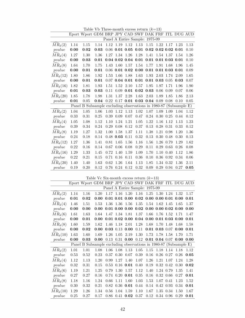
Table Vb Three-month excess return (k=13)Eport Wport GDM BRP JPY CAD SWF DAK FRF ITL DUG AUD

Panel A Entire Sample: 1975-09

M̂Rk(2) 1.14 1.15 1.14 1.12 1.19 1.12 1.13 1.15 1.22 1.17 1.23 1.13pvalue 0.00 0.02 0.03 0.06 0.01 0.05 0.01 0.02 0.02 0.02 0.01 0.10

M̂Rk(4) 1.27 1.30 1.36 1.27 1.34 1.26 1.28 1.41 1.54 1.37 1.54 1.26pvalue 0.00 0.03 0.01 0.04 0.02 0.04 0.01 0.01 0.01 0.03 0.01 0.10

M̂Rk(8) 1.64 1.70 1.75 1.43 1.60 1.57 1.54 1.77 1.91 1.68 1.96 1.45pvalue 0.00 0.01 0.01 0.06 0.01 0.02 0.00 0.01 0.01 0.03 0.01 0.09

M̂Rk(12) 1.80 1.86 1.92 1.53 1.66 1.88 1.63 1.93 2.03 1.74 2.09 1.65pvalue 0.00 0.01 0.01 0.07 0.04 0.01 0.01 0.01 0.03 0.05 0.03 0.07

M̂Rk(16) 1.82 1.81 1.93 1.51 1.52 2.10 1.57 1.95 1.97 1.71 1.96 1.90pvalue 0.01 0.03 0.03 0.11 0.09 0.01 0.02 0.03 0.06 0.09 0.07 0.06

M̂Rk(20) 1.85 1.78 1.98 1.31 1.37 2.28 1.63 2.03 1.89 1.85 1.86 2.13pvalue 0.01 0.05 0.04 0.22 0.17 0.01 0.03 0.04 0.09 0.08 0.10 0.05

Panel B Subsample excluding observations in 1980-87 (Subsample E)

M̂Rk(2) 1.04 1.05 1.06 1.03 1.12 1.13 1.02 1.07 1.09 1.09 1.04 1.12pvalue 0.33 0.31 0.25 0.39 0.09 0.07 0.47 0.24 0.30 0.25 0.44 0.12

M̂Rk(4) 1.05 1.08 1.12 1.10 1.24 1.21 1.05 1.22 1.16 1.12 1.13 1.23pvalue 0.39 0.34 0.24 0.29 0.08 0.12 0.37 0.13 0.28 0.31 0.33 0.12

M̂Rk(8) 1.19 1.27 1.32 1.00 1.58 1.37 1.11 1.38 1.21 0.98 1.20 1.36pvalue 0.24 0.18 0.14 0.48 0.03 0.11 0.32 0.13 0.30 0.48 0.30 0.13

M̂Rk(12) 1.27 1.36 1.41 0.81 1.65 1.56 1.16 1.56 1.26 0.79 1.29 1.62pvalue 0.22 0.16 0.14 0.67 0.06 0.08 0.29 0.11 0.29 0.63 0.26 0.08

M̂Rk(16) 1.29 1.33 1.45 0.72 1.40 1.59 1.09 1.70 1.10 0.40 1.12 1.86pvalue 0.22 0.21 0.15 0.71 0.16 0.11 0.36 0.10 0.36 0.92 0.34 0.06

M̂Rk(20) 1.40 1.40 1.63 0.62 1.26 1.64 1.13 1.85 1.34 0.32 1.36 2.11pvalue 0.19 0.20 0.12 0.76 0.24 0.12 0.32 0.09 0.29 0.94 0.27 0.05

Table Vc Six-month excess return (k=13)Eport Wport GDM BRP JPY CAD SWF DAK FRF ITL DUG AUD

Panel A Entire Sample: 1975-09

M̂Rk(2) 1.14 1.16 1.20 1.17 1.16 1.20 1.16 1.25 1.30 1.24 1.32 1.17pvalue 0.01 0.02 0.00 0.01 0.01 0.00 0.02 0.00 0.00 0.01 0.00 0.01

M̂Rk(4) 1.46 1.51 1.53 1.36 1.36 1.56 1.35 1.54 1.62 1.45 1.65 1.37pvalue 0.00 0.00 0.00 0.01 0.00 0.00 0.02 0.00 0.00 0.02 0.00 0.00

M̂Rk(6) 1.61 1.63 1.64 1.47 1.34 1.81 1.37 1.66 1.76 1.52 1.71 1.47pvalue 0.00 0.01 0.00 0.01 0.02 0.00 0.04 0.00 0.01 0.03 0.00 0.01

M̂Rk(8) 1.60 1.59 1.62 1.46 1.18 2.01 1.28 1.68 1.70 1.48 1.68 1.58pvalue 0.00 0.02 0.00 0.03 0.13 0.00 0.11 0.01 0.03 0.07 0.00 0.01

M̂Rk(10) 1.63 1.60 1.69 1.26 1.05 2.19 1.30 1.73 1.78 1.58 1.70 1.71pvalue 0.00 0.03 0.00 0.13 0.31 0.00 0.12 0.01 0.04 0.07 0.00 0.00

Panel B Subsample excluding observations in 1980-87 (Subsample E)

M̂Rk(2) 1.01 1.01 1.08 1.06 1.08 1.13 1.05 1.15 1.18 1.14 1.18 1.12pvalue 0.53 0.52 0.23 0.37 0.30 0.07 0.39 0.16 0.26 0.27 0.26 0.05

M̂Rk(4) 1.12 1.13 1.20 0.99 1.27 1.40 1.07 1.26 1.21 1.07 1.24 1.28pvalue 0.32 0.31 0.15 0.53 0.16 0.01 0.40 0.19 0.32 0.42 0.30 0.02

M̂Rk(6) 1.19 1.21 1.25 0.79 1.30 1.57 1.12 1.40 1.24 0.79 1.35 1.41pvalue 0.27 0.27 0.16 0.74 0.20 0.01 0.35 0.16 0.32 0.66 0.27 0.01

M̂Rk(8) 1.18 1.16 1.24 0.66 1.11 1.60 1.03 1.53 1.07 0.41 1.23 1.52pvalue 0.30 0.32 0.21 0.82 0.36 0.01 0.44 0.14 0.42 0.93 0.34 0.01

M̂Rk(10) 1.29 1.26 1.34 0.56 1.04 1.59 1.10 1.67 1.35 0.34 1.50 1.67pvalue 0.25 0.27 0.17 0.86 0.41 0.02 0.37 0.12 0.34 0.96 0.29 0.01

42

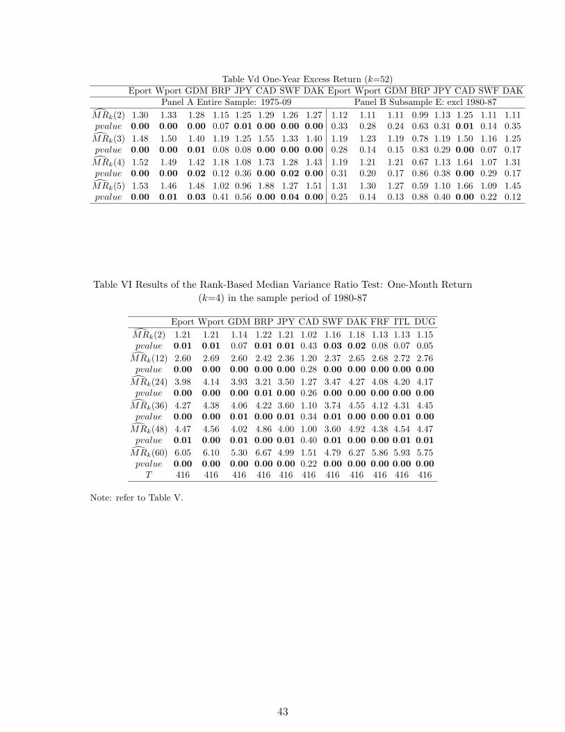
Table Vd One-Year Excess Return (k=52)Eport Wport GDM BRP JPY CAD SWF DAK Eport Wport GDM BRP JPY CAD SWF DAK

Panel A Entire Sample: 1975-09 Panel B Subsample E: excl 1980-87

M̂Rk(2) 1.30 1.33 1.28 1.15 1.25 1.29 1.26 1.27 1.12 1.11 1.11 0.99 1.13 1.25 1.11 1.11pvalue 0.00 0.00 0.00 0.07 0.01 0.00 0.00 0.00 0.33 0.28 0.24 0.63 0.31 0.01 0.14 0.35

M̂Rk(3) 1.48 1.50 1.40 1.19 1.25 1.55 1.33 1.40 1.19 1.23 1.19 0.78 1.19 1.50 1.16 1.25pvalue 0.00 0.00 0.01 0.08 0.08 0.00 0.00 0.00 0.28 0.14 0.15 0.83 0.29 0.00 0.07 0.17

M̂Rk(4) 1.52 1.49 1.42 1.18 1.08 1.73 1.28 1.43 1.19 1.21 1.21 0.67 1.13 1.64 1.07 1.31pvalue 0.00 0.00 0.02 0.12 0.36 0.00 0.02 0.00 0.31 0.20 0.17 0.86 0.38 0.00 0.29 0.17

M̂Rk(5) 1.53 1.46 1.48 1.02 0.96 1.88 1.27 1.51 1.31 1.30 1.27 0.59 1.10 1.66 1.09 1.45pvalue 0.00 0.01 0.03 0.41 0.56 0.00 0.04 0.00 0.25 0.14 0.13 0.88 0.40 0.00 0.22 0.12

Table VI Results of the Rank-Based Median Variance Ratio Test: One-Month Return

(k=4) in the sample period of 1980-87

Eport Wport GDM BRP JPY CAD SWF DAK FRF ITL DUG

M̂Rk(2) 1.21 1.21 1.14 1.22 1.21 1.02 1.16 1.18 1.13 1.13 1.15pvalue 0.01 0.01 0.07 0.01 0.01 0.43 0.03 0.02 0.08 0.07 0.05

M̂Rk(12) 2.60 2.69 2.60 2.42 2.36 1.20 2.37 2.65 2.68 2.72 2.76pvalue 0.00 0.00 0.00 0.00 0.00 0.28 0.00 0.00 0.00 0.00 0.00

M̂Rk(24) 3.98 4.14 3.93 3.21 3.50 1.27 3.47 4.27 4.08 4.20 4.17pvalue 0.00 0.00 0.00 0.01 0.00 0.26 0.00 0.00 0.00 0.00 0.00

M̂Rk(36) 4.27 4.38 4.06 4.22 3.60 1.10 3.74 4.55 4.12 4.31 4.45pvalue 0.00 0.00 0.01 0.00 0.01 0.34 0.01 0.00 0.00 0.01 0.00

M̂Rk(48) 4.47 4.56 4.02 4.86 4.00 1.00 3.60 4.92 4.38 4.54 4.47pvalue 0.01 0.00 0.01 0.00 0.01 0.40 0.01 0.00 0.00 0.01 0.01

M̂Rk(60) 6.05 6.10 5.30 6.67 4.99 1.51 4.79 6.27 5.86 5.93 5.75pvalue 0.00 0.00 0.00 0.00 0.00 0.22 0.00 0.00 0.00 0.00 0.00

T 416 416 416 416 416 416 416 416 416 416 416

Note: refer to Table V.

43

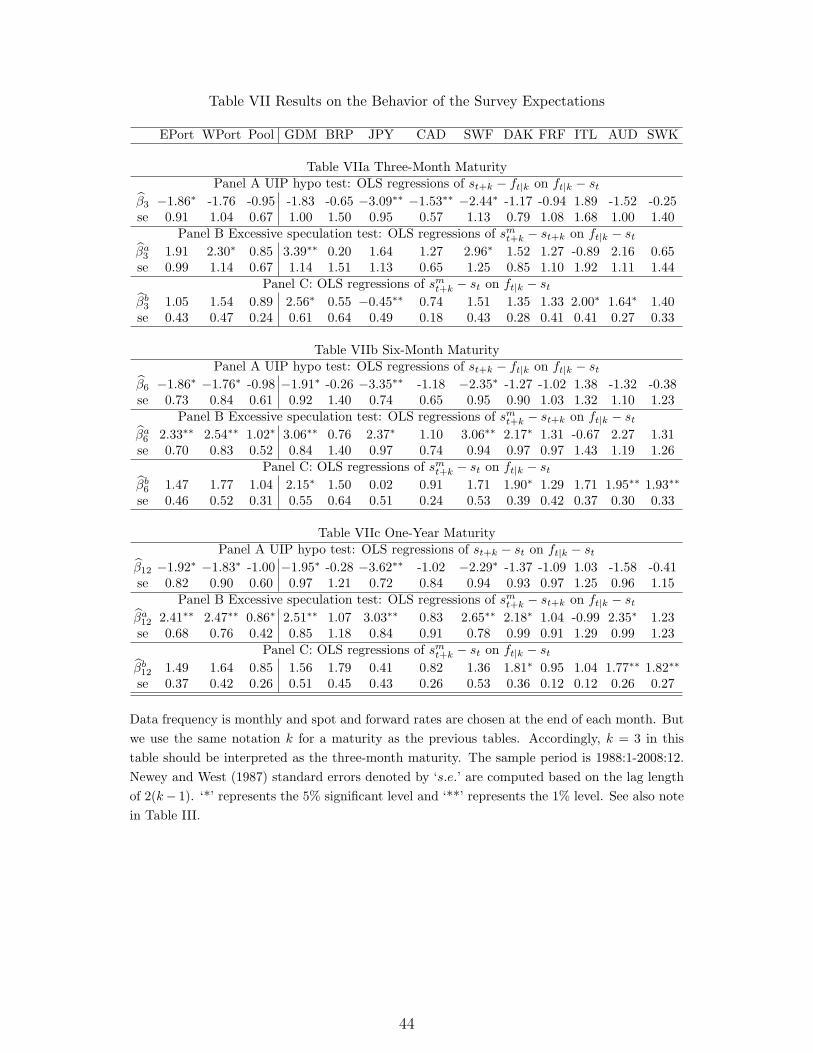
Table VII Results on the Behavior of the Survey Expectations

EPort WPort Pool GDM BRP JPY CAD SWF DAK FRF ITL AUD SWK

Table VIIa Three-Month MaturityPanel A UIP hypo test: OLS regressions of st+k − ft|k on ft|k − st

β̂3 −1.86∗ -1.76 -0.95 -1.83 -0.65 −3.09∗∗ −1.53∗∗ −2.44∗ -1.17 -0.94 1.89 -1.52 -0.25se 0.91 1.04 0.67 1.00 1.50 0.95 0.57 1.13 0.79 1.08 1.68 1.00 1.40

Panel B Excessive speculation test: OLS regressions of smt+k − st+k on ft|k − stβ̂a3 1.91 2.30∗ 0.85 3.39∗∗ 0.20 1.64 1.27 2.96∗ 1.52 1.27 -0.89 2.16 0.65se 0.99 1.14 0.67 1.14 1.51 1.13 0.65 1.25 0.85 1.10 1.92 1.11 1.44

Panel C: OLS regressions of smt+k − st on ft|k − stβ̂b3 1.05 1.54 0.89 2.56∗ 0.55 −0.45∗∗ 0.74 1.51 1.35 1.33 2.00∗ 1.64∗ 1.40se 0.43 0.47 0.24 0.61 0.64 0.49 0.18 0.43 0.28 0.41 0.41 0.27 0.33

Table VIIb Six-Month MaturityPanel A UIP hypo test: OLS regressions of st+k − ft|k on ft|k − st

β̂6 −1.86∗ −1.76∗ -0.98 −1.91∗ -0.26 −3.35∗∗ -1.18 −2.35∗ -1.27 -1.02 1.38 -1.32 -0.38se 0.73 0.84 0.61 0.92 1.40 0.74 0.65 0.95 0.90 1.03 1.32 1.10 1.23

Panel B Excessive speculation test: OLS regressions of smt+k − st+k on ft|k − stβ̂a6 2.33∗∗ 2.54∗∗ 1.02∗ 3.06∗∗ 0.76 2.37∗ 1.10 3.06∗∗ 2.17∗ 1.31 -0.67 2.27 1.31se 0.70 0.83 0.52 0.84 1.40 0.97 0.74 0.94 0.97 0.97 1.43 1.19 1.26

Panel C: OLS regressions of smt+k − st on ft|k − stβ̂b6 1.47 1.77 1.04 2.15∗ 1.50 0.02 0.91 1.71 1.90∗ 1.29 1.71 1.95∗∗ 1.93∗∗

se 0.46 0.52 0.31 0.55 0.64 0.51 0.24 0.53 0.39 0.42 0.37 0.30 0.33

Table VIIc One-Year MaturityPanel A UIP hypo test: OLS regressions of st+k − st on ft|k − st

β̂12 −1.92∗ −1.83∗ -1.00 −1.95∗ -0.28 −3.62∗∗ -1.02 −2.29∗ -1.37 -1.09 1.03 -1.58 -0.41se 0.82 0.90 0.60 0.97 1.21 0.72 0.84 0.94 0.93 0.97 1.25 0.96 1.15

Panel B Excessive speculation test: OLS regressions of smt+k − st+k on ft|k − stβ̂a12 2.41∗∗ 2.47∗∗ 0.86∗ 2.51∗∗ 1.07 3.03∗∗ 0.83 2.65∗∗ 2.18∗ 1.04 -0.99 2.35∗ 1.23se 0.68 0.76 0.42 0.85 1.18 0.84 0.91 0.78 0.99 0.91 1.29 0.99 1.23

Panel C: OLS regressions of smt+k − st on ft|k − stβ̂b12 1.49 1.64 0.85 1.56 1.79 0.41 0.82 1.36 1.81∗ 0.95 1.04 1.77∗∗ 1.82∗∗

se 0.37 0.42 0.26 0.51 0.45 0.43 0.26 0.53 0.36 0.12 0.12 0.26 0.27

Data frequency is monthly and spot and forward rates are chosen at the end of each month. But

we use the same notation k for a maturity as the previous tables. Accordingly, k = 3 in this

table should be interpreted as the three-month maturity. The sample period is 1988:1-2008:12.

Newey and West (1987) standard errors denoted by ‘s.e.’ are computed based on the lag length

of 2(k− 1). ‘*’ represents the 5% significant level and ‘**’ represents the 1% level. See also note

in Table III.

44

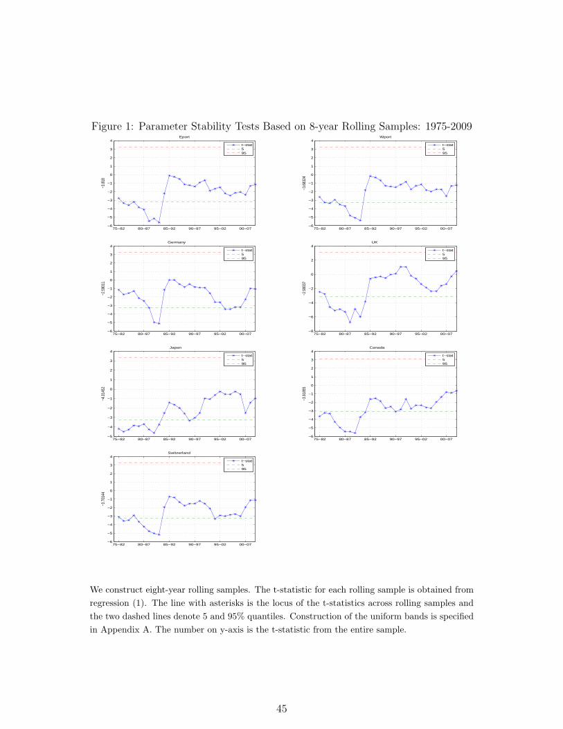
Figure 1: Parameter Stability Tests Based on 8-year Rolling Samples: 1975-2009

75−82 80−87 85−92 90−97 95−02 00−07−6

−5

−4

−3

−2

−1

0

1

2

3

4

−3.8

18

Eport

t−stat595

75−82 80−87 85−92 90−97 95−02 00−07−6

−5

−4

−3

−2

−1

0

1

2

3

4

−3.6

8324

Wport

t−stat595

75−82 80−87 85−92 90−97 95−02 00−07−6

−5

−4

−3

−2

−1

0

1

2

3

4

−2.5

9011

Germany

t−stat595

75−82 80−87 85−92 90−97 95−02 00−07−8

−6

−4

−2

0

2

4

−2.9

0037

UK

t−stat595

75−82 80−87 85−92 90−97 95−02 00−07−5

−4

−3

−2

−1

0

1

2

3

4

−4.0

1452

Japan

t−stat595

75−82 80−87 85−92 90−97 95−02 00−07−6

−5

−4

−3

−2

−1

0

1

2

3

4

−3.9

1855

Canada

t−stat595

75−82 80−87 85−92 90−97 95−02 00−07−6

−5

−4

−3

−2

−1

0

1

2

3

4

−3.7

0144

Switzerland

t−stat595

We construct eight-year rolling samples. The t-statistic for each rolling sample is obtained from

regression (1). The line with asterisks is the locus of the t-statistics across rolling samples and

the two dashed lines denote 5 and 95% quantiles. Construction of the uniform bands is specified

in Appendix A. The number on y-axis is the t-statistic from the entire sample.

45

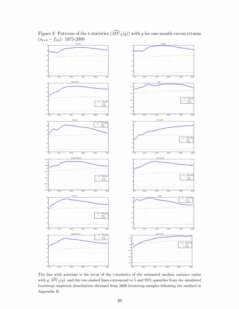
Figure 2: Patterns of the t-statistics (M̂V k(q)) with q for one-month excess returns(st+4 − ft|4): 1975-2009

2m 12m 24m 36m 48m 60m−2

−1

0

1

2

3

4Eport

2m 12m 24m 36m 48m 60m−2

−1

0

1

2

3

4Wport

2m 12m 24m 36m 48m 60m−2

−1

0

1

2

3

4

5Germany

MVk(q)

0.50.95

2m 12m 24m 36m 48m 60m−1.5

−1

−0.5

0

0.5

1

1.5

2

2.5

3UK

MVk(q)

0.50.95

2m 12m 24m 36m 48m 60m−2

−1

0

1

2

3

4

5Japan

MV

k(q)

0.50.95

2m 12m 24m 36m 48m 60m−2

−1

0

1

2

3

4

5Canada

MVk(q)

0.50.95

2m 12m 24m 36m 48m 60m−1.5

−1

−0.5

0

0.5

1

1.5

2

2.5

3

3.5Switzerland

MVk(q)

0.50.95

2m 12m 24m 36m 48m 60m−2

−1

0

1

2

3

4

5Denmark

MVk(q)

0.50.95

2m 12m 24m 36m 48m 60m−2

−1

0

1

2

3

4France

MVk(q)

0.50.95

2m 12m 24m 36m 48m 60m−2

−1

0

1

2

3

4Italy

MVk(q)

0.50.95

2m 12m 24m 36m 48m 60m−2

−1

0

1

2

3

4

5Netherland

MVk(q)

0.50.95

2m 12m 24m 36m 48m 60m−2

−1.5

−1

−0.5

0

0.5

1

1.5

2

2.5

3Austrailia

MVk(q)

0.50.95

The line with asterisks is the locus of the t-statistics of the estimated median variance ratios

with q, M̂V k(q), and the two dashed lines correspond to 5 and 95% quantiles from the simulated

bootstrap empirical distribution obtained from 5000 bootstrap samples following the method in

Appendix B.

46

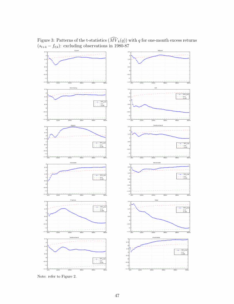
Figure 3: Patterns of the t-statistics (M̂V k(q)) with q for one-month excess returns(st+4 − ft|4): excluding observations in 1980-87

2m 12m 24m 36m 48m 60m−1.5

−1

−0.5

0

0.5

1

1.5

2

2.5Eport

2m 12m 24m 36m 48m 60m−1.5

−1

−0.5

0

0.5

1

1.5

2

2.5Wport

2m 12m 24m 36m 48m 60m−1.5

−1

−0.5

0

0.5

1

1.5

2

2.5Germany

MVk(q)

0.50.95

2m 12m 24m 36m 48m 60m−1.5

−1

−0.5

0

0.5

1

1.5

2

2.5UK

MVk(q)

0.50.95

2m 12m 24m 36m 48m 60m−1.5

−1

−0.5

0

0.5

1

1.5

2

2.5

3

3.5Japan

MVk(q)

0.50.95

2m 12m 24m 36m 48m 60m−1.5

−1

−0.5

0

0.5

1

1.5

2

2.5Switzerland

MVk(q)

0.50.95

2m 12m 24m 36m 48m 60m−1.5

−1

−0.5

0

0.5

1

1.5

2

2.5

3Canada

MVk(q)

0.50.95

2m 12m 24m 36m 48m 60m−2

−1.5

−1

−0.5

0

0.5

1

1.5

2

2.5

3Denmark

MVk(q)

0.50.95

2m 12m 24m 36m 48m 60m−1.5

−1

−0.5

0

0.5

1

1.5

2

2.5France

MVk(q)

0.50.95

2m 12m 24m 36m 48m 60m−1.5

−1

−0.5

0

0.5

1

1.5

2

2.5Italy

MVk(q)

0.50.95

2m 12m 24m 36m 48m 60m−1.5

−1

−0.5

0

0.5

1

1.5

2

2.5Netherland

MVk(q)

0.50.95

2m 12m 24m 36m 48m 60m−1.5

−1

−0.5

0

0.5

1

1.5

2

2.5

3Austrailia

MVk(q)

0.50.95

Note: refer to Figure 2.

47

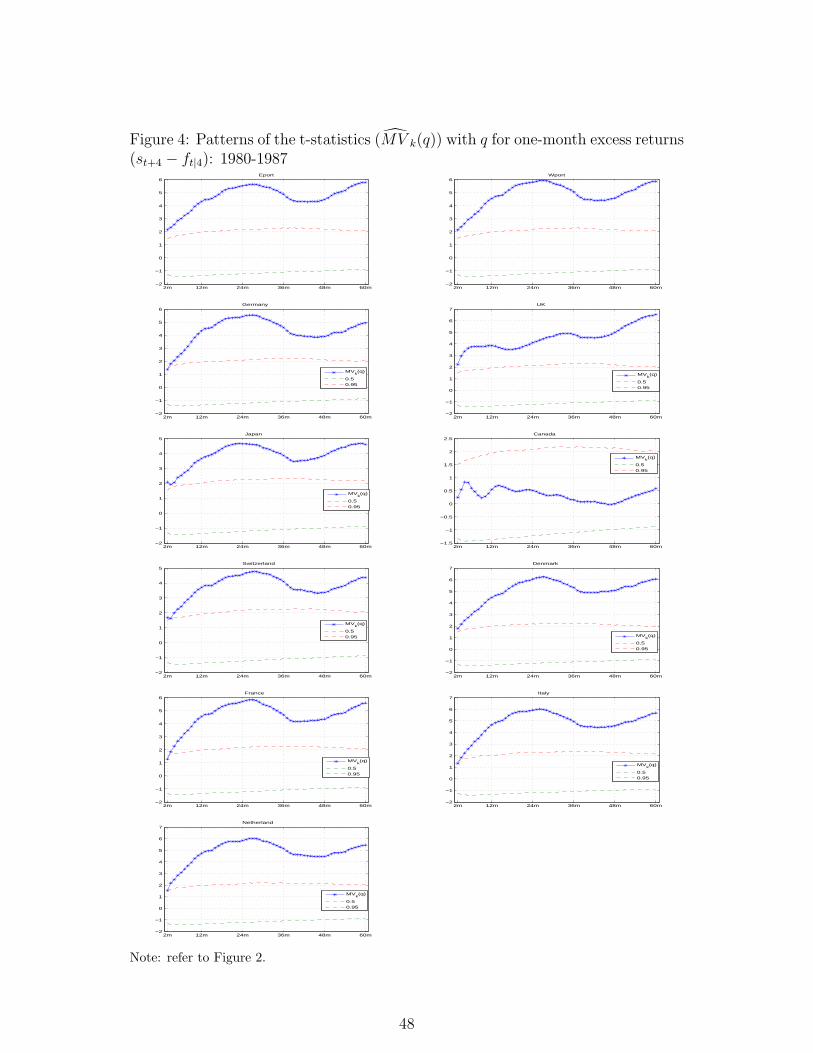
Figure 4: Patterns of the t-statistics (M̂V k(q)) with q for one-month excess returns(st+4 − ft|4): 1980-1987

2m 12m 24m 36m 48m 60m−2

−1

0

1

2

3

4

5

6Eport

2m 12m 24m 36m 48m 60m−2

−1

0

1

2

3

4

5

6Wport

2m 12m 24m 36m 48m 60m−2

−1

0

1

2

3

4

5

6Germany

MVk(q)

0.50.95

2m 12m 24m 36m 48m 60m−2

−1

0

1

2

3

4

5

6

7UK

MVk(q)

0.50.95

2m 12m 24m 36m 48m 60m−2

−1

0

1

2

3

4

5Japan

MVk(q)

0.50.95

2m 12m 24m 36m 48m 60m−1.5

−1

−0.5

0

0.5

1

1.5

2

2.5Canada

MVk(q)

0.50.95

2m 12m 24m 36m 48m 60m−2

−1

0

1

2

3

4

5Switzerland

MVk(q)

0.50.95

2m 12m 24m 36m 48m 60m−2

−1

0

1

2

3

4

5

6

7Denmark

MVk(q)

0.50.95

2m 12m 24m 36m 48m 60m−2

−1

0

1

2

3

4

5

6France

MVk(q)

0.50.95

2m 12m 24m 36m 48m 60m−2

−1

0

1

2

3

4

5

6

7Italy

MVk(q)

0.50.95

2m 12m 24m 36m 48m 60m−2

−1

0

1

2

3

4

5

6

7Netherland

MVk(q)

0.50.95

Note: refer to Figure 2.

48

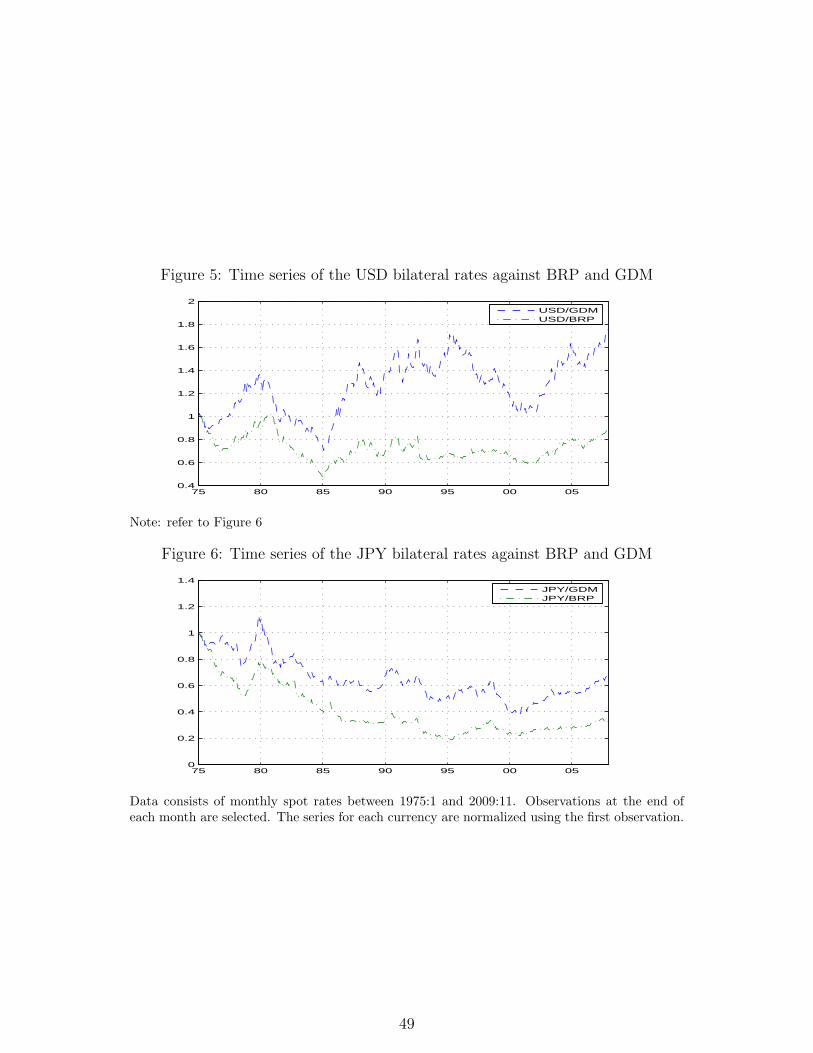
Figure 5: Time series of the USD bilateral rates against BRP and GDM

75 80 85 90 95 00 050.4

0.6

0.8

1

1.2

1.4

1.6

1.8

2

USD/GDMUSD/BRP

Note: refer to Figure 6

Figure 6: Time series of the JPY bilateral rates against BRP and GDM

75 80 85 90 95 00 050

0.2

0.4

0.6

0.8

1

1.2

1.4

JPY/GDMJPY/BRP

Data consists of monthly spot rates between 1975:1 and 2009:11. Observations at the end ofeach month are selected. The series for each currency are normalized using the first observation.

49

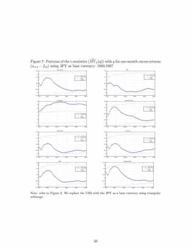
Figure 7: Patterns of the t-statistics (M̂V k(q)) with q for one-month excess returns(st+4 − ft|4) using JPY as base currency: 1980-1987

2m 12m 24m 36m 48m 60m−1.5

−1

−0.5

0

0.5

1

1.5

2

2.5Germany

MVk(q)

0.50.95

2m 12m 24m 36m 48m 60m−1.5

−1

−0.5

0

0.5

1

1.5

2

2.5UK

MVk(q)

0.50.95

2m 12m 24m 36m 48m 60m−2

−1

0

1

2

3

4

5Canada

MVk(q)

0.50.95

2m 12m 24m 36m 48m 60m−1.5

−1

−0.5

0

0.5

1

1.5

2

2.5Switzerland

MVk(q)

0.50.95

2m 12m 24m 36m 48m 60m−1.5

−1

−0.5

0

0.5

1

1.5

2

2.5Denmark

MVk(q)

0.50.95

2m 12m 24m 36m 48m 60m−1.5

−1

−0.5

0

0.5

1

1.5

2

2.5France

MVk(q)

0.50.95

2m 12m 24m 36m 48m 60m−1.5

−1

−0.5

0

0.5

1

1.5

2

2.5Italy

MVk(q)

0.50.95

2m 12m 24m 36m 48m 60m−1.5

−1

−0.5

0

0.5

1

1.5

2

2.5Netherland

MVk(q)

0.50.95

Note: refer to Figure 2. We replace the USD with the JPY as a base currency using triangulararbitrage.

50