Electronic copy available at: https://ssrn.com/abstract=2692892

The Leading Premium

M. Max Croce Tatyana Marchuk Christian Schlag∗

————————————————————————————————————–

Abstract

In this paper, we compute conditional measures of lead-lag relationships between GDPgrowth and industry-level cash-flow growth in the US. Our results show that firms inleading industries pay an average annualized return 4% higher than that of firms inlagging industries. The difference in the returns of leading and lagging firms is pricedin the cross section of equity returns, even after we control for a large number of riskfactors. This finding can be rationalized in a model in which (a) agents price growthnews shocks, and (b) leading industries provide valuable resolution of uncertainty aboutthe growth prospects of lagging industries.

JEL classification: G10; E32; E44.First draft : Sept. 16, 2015. This draft : December 11, 2017.

————————————————————————————————————–

∗Croce is affiliated with the Kenan-Flagler Business School, University of North Carolina at Chapel Hill,and CEPR. Marchuk is affiliated with the Finance Department of BI Norwegian Business School. Schlag isaffiliated with the Finance Department and Research Center SAFE at Goethe University Frankfurt . Wethank E. Farhi, C. Julliard, and M. Yogo, and S. van Nieuwerburgh for early feedback. We are very gratefulto our discussants Thomas Q. Pedersen and Jun Li. We also thank the seminar participants at the CEPRmeetings, WFA Meetings, SED Mettings, Econometric Society Meetings, SGF Meeting, Macro-Finance Soci-ety Meeting, Kenan-Flagler Business School, Tilburg University (Finance), Maastricht University (Finance),Hong Kong University of Science and Technology, Toronto University, Carlson School of Management andSAFE.

Electronic copy available at: https://ssrn.com/abstract=2692892

1 Introduction

Different macroeconomic aggregates go through economic cycles with different timings (see,

among others, Stock and Watson 1989, 2002; and Estrella and Mishkin 1998). Variables

that respond promptly to exogenous shocks are denoted as “leading,” whereas variables that

adjust with delay are called “lagging.”1 Thus far, the empirical macroeconomic literature

has focused mainly on leads and lags of aggregate indicators. Little is yet known about leads

and lags across firms operating in different segments of the economy.

In this paper, we document the existence of a significant lead-lag structure in fundamen-

tal cash flows across industries. This structure is relevant to the explanation of the cross

section of stock returns, as leading industries pay a higher average stock return than lagging

industries, in the order of about 4% per year. This figure remains as significant as both the

equity and the value premium even after controlling for a large number of related factors in

time-series tests.

In order to perform also cross-sectional tests, we construct a risk factor by considering

a zero-dollar investment strategy long in a portfolio of leading industries and short in a

portfolio of lagging industries. We denote the returns of this portfolio as the LL factor.

A formal GMM estimation of a linear pricing model with both the LL and the Fama and

French (1993) three factors (FF3 hereafter) shows that LL is priced in our cross section of

industry portfolio returns, suggesting that we are focusing on a novel firm characteristic.

Furthermore, the LL factor has a significant loading in the model-implied stochastic dis-

count factor, implying that asset prices are sensitive to the timing of economic fluctuations.

Consistent with this intuition, we show that our findings are an anomaly in a model with

time-additive preferences, whereas a model with news shocks and preferences for early reso-

lution of uncertainty explains our cross-sectional results. This is because leading industries

provide valuable anticipated resolution of uncertainty for industries that go through ag-

gregate economic fluctuations with delay. As a result, lagging firms bear less conditional

cash-flow uncertainty and, by no arbitrage, ceteris paribus have a higher price (or, equiva-

lently, a lower yield). Leading firms, in contrast, play the role of early indicators like canaries

in a coal mine and pay a higher equity yield.

More specifically, we compute rolling-window correlations between US output growth and

leads and lags of operating income growth at an industry level. Data are quarterly and span

the period 1972–2012. We consider 17,000 firms, which we aggregate to industries using the

industry classification scheme obtained from Kenneth French’s website.2 In each quarter, we

1For example, both bond yields and the stock market index tend to be leading indicators with respectto domestic output, as they forecast future recessions and booms. Unemployment, in contrast, is a laggingindicator.

2See, for example, http://mba.tuck.dartmouth.edu/pages/faculty/ken.french/Data_Library/

det_30_ind_port.html.

1

Electronic copy available at: https://ssrn.com/abstract=2692892

focus on a four-quarter window of leads and lags. After identifying the highest correlation in

absolute value within this window, we assign the corresponding lead/lag indicator (ranging

from −4 to +4) to the industry of interest. Note that this approach uses only past data to

compute the cross-correlograms, and hence it can be used to construct an implementable

investment strategy in real-time.

This procedure gives us a panel of quarterly leading-lagging indicators spanning 41 years

of data. In each sample period, we find sizable heterogeneity in these indicators across our

industries. Focusing on individual industries, we also observe considerable fluctuations in

the time series of their lead and lag indicators, i.e., an industry may be leading in a specific

period, but lagging in another. We speculate that this may depend on the origin of the

underlying economic shock affecting firms. As an example, the firms leading during an IT

boom do not necessarily lead during a financial crisis. In Appendix D, we formalize this idea

in a multisector economy in which cash flows are affected by infrequently arriving shocks that

slowly diffuse across all sectors and turn into aggregate production growth shocks. Possible

microfoundations of our diffusion are provided in Caplin and Leahy (1993, 1994).

We then sort our firms according to their industry-level lead-lag indicator and form three

portfolios, which are dynamically updated at a quarterly frequency. In each quarter, we

make sure that the extreme portfolios have a market capitalization share of at least 15%,

so that our results are not driven by a subset of small and illiquid firms. According to this

standard procedure, we find a monotonic positive relation between the average returns and

the leading indicators of our portfolios. Our LL factor has an annualized average return of

4%, which remains sizeable and significant after adjusting, for example, for the FF3 factors.

The industries with the highest exposure to our LL factor are also the ones whose operating

income strongly leads national output.

Furthermore, we show that our findings are statistically significant after double-sorting on

LL exposure and either the book-to-market ratio or size, implying that the LL premium is a

broad phenomenon in the cross section. We also show that our risk factor is not subsumed

by other cyclical factors such as investment minus consumption (Kogan and Papanikolaou

2014), durability (Gomes et al. 2009), industry-momentum (Moskowitz and Grinblatt 1999),

industry betting-against-beta (Asness et al. 2014), the five factors suggested by Fama and

French 2015, and the q-Factors (Hou et al. 2015a, b).

We use a stylized example to build up intuition and show via a simple no arbitrage

argument that our leading premium should be related to the forward equity yield on leading

industry dividends (Binsbergen et al. 2013). This result is important because it suggests that

models that produce a substantial positive spread between bond and zero-coupon equity

yields may rationalize the leading premium. For the sake of analytical tractability, we

abstract away from investment decisions (Albuquerque and Miao 2014) and consider the

endowment economy of Bansal and Yaron (2004), in which consumption growth is subject to

2

persistent news shocks, which are directly priced by Epstein and Zin (1989) (EZ) preferences.

In the spirit of Bansal et al. (2005), we use this model to price a cross section of cash

flows that differ from each other in their lead-lag structure, with the goal of explaining our

leading premium. Specifically, we project consumption growth in the US on the Jurado et al.

(2015) factors to identify the aggregate long-run growth component and disentangle it from

short-run growth shocks. We then compute the cash flows from investing in our leading and

lagging portfolios, respectively. In a second step, we project the cash-flow growth rates on

leads and lags of the components of consumption growth.

The relevance of this step is twofold. On the one hand, we identify the lead-lag structure of

cash flows and better characterize the composition of the representative agent’s information

set, that is, we identify how much advance information the agent can obtain from the leading

cash flows. On the other hand, this procedure also accounts for heterogeneity in the exposure

of cash flows to fundamental consumption growth shocks.

As mentioned above, prior manuscripts have already documented that heterogeneous

exposure to contemporaneous news shocks can explain the value premium (see, among others,

Bansal et al. 2005). We differ from prior studies by showing that heterogeneous timing of

exposure to news shocks explains the leading premium. Consistent with the data, when

calibrating our cash-flow processes we control for heterogeneous exposure to fundamental

shocks in order to obtain the most proper and conservative prediction for the model-implied

leading premium.

In the data, we find that the cash flows of the leading portfolio provide information about

the long-run consumption growth component 27 quarters ahead. The time gap increases to

47 quarters with respect to the lagging portfolio, implying that this latter portfolio benefits

substantially from early resolution of uncertainty. Under a standard calibration of the model

consistent with our data, the implied leading premium is 3.10%, a figure very close to our

estimate and almost completely driven by the long-run shocks in our model. The short-run

shocks play a role only when we create a synthetic cross section of stocks that differ in both

their lead-lag structure and their exposure to short-run risk, as in the data. In this case,

our equilibrium cross section of returns has a two-factor representation, and the implied

synthetic LL factor is priced in addition to the market factor, consistent with our empirical

evidence.

We conclude our analysis with a counterfactual experiment designed to quantify the wel-

fare value of the advance information provided by the leading industries. Specifically, we

look at an economy calibrated as in our benchmark case, where we simply remove future

long-run consumption growth news from the information set of the agent. Put differently,

we retain the same amount of consumption long-run risk, but we pretend that there is no

leading portfolio providing advance information about it. We find that the welfare benefits

of the information stemming from our cross section of industries are worth 6% of life-time

3

consumption. In order to correctly interpret this result, we run the Lucas (1987) experiment

in our economy and find that the welfare benefits of removing all uncertainty are in the

order of 65%.3 Therefore, the advance information that we identify in the cross section of

industries represents less than 10% of the maximum attainable welfare benefits.

Epstein et al. (2014) point out that in the Bansal and Yaron (2004) model, the Lucas

welfare benefits originate mainly from full resolution of uncertainty, not from the removal

of deterministic fluctuations. Our computations show that early resolution of uncertainty in

the cross section of industries is simultaneously valuable but limited, as it carries a strong

market price of risk but reveals future long-run consumption dynamics over a relatively short

horizon.

Patton and Verado (2012) and Savor and Wilson (2016) document the existence of higher

risk for firms that release advance information by announcing their earnings. Ai and Bansal

(2015) provide a theoretical foundation of the announcement premiums, including those in

Savor and Wilson (2013). Kadan and Manela (2016) estimate the value of information using

options. Our main goal is to empirically quantify the relevance of heterogeneity in the timing

of exposure of cash flows to aggregate shocks for the cross section of industry returns. Our

results are significant beyond announcement events.

Koijen et al. (2017) show that the Cochrane and Piazzesi (2005) factor is a strong predictor

of economic activity, with a lead of up to 10 quarters relative to GDP growth. Working with

the cross section of bond and equity returns, they provide evidence suggesting that book-

to-market-sorted stocks contain information about future growth. Similarly to them, we

show that the price-dividend ratio of leading firms forecasts economic activity, even after

controlling for other common predictors. We differ from their work in our focus on industries,

our empirical and theoretical characterization of the leading premium, and the assessment

of the welfare benefits stemming from advance information about future growth.

Based on the observation that some components of aggregate consumption are more

cyclical than others, Gomes et al. (2009) show that durable good producers have cash flows

both more volatile and more highly correlated with aggregate consumption than those of

firms producing nondurables and services. Furthermore, output durability is a priced factor

in the cross section of equity returns. We differ from this study in our attention toward

heterogeneity in the timing of exposure to fundamental shocks.

Fama and French (1997) find that the FF3 model exhibits only modest performance in

explaining the cross section of industry returns. Our LL factor significantly improves our

ability to explain industry returns above and beyond what is documented in other studies.

Hong et al. (2007) investigate whether high-frequency industry returns can forecast ex-

cess returns on the CRSP market index. They find evidence of predictability, but only on

3This figure is much smaller than that in Ai (2007) and Croce (2013), as our consumption process iscalibrated according to post-1972 data, i.e., its volatility is moderate.

4

very short horizons of one or two months. In contrast to previous studies, our empirical

investigation is based on cash-flow fundamentals and focuses on longer time horizons. In the

context of a rational equilibrium model in which anticipated news is priced, there exists a

link between the timing of cash-flow exposure and expected returns. Our endogenous cross

section of returns features no lead-lag structure, that is, all returns move simultaneously, but

with different endogenous sensitivities.

As we show by means of a stylized example in section 3, the existence of a leading premium

does not depend on the slope of the equity yield curve, but just on the spread between the

the equity and the risk-free bond yield curve. Richer settings like those suggested by Lettau

and Wachter (2007, 2011), Croce et al. (2014), and Ai et al. (2017), Belo et al. (2014) are

consistent with the empirical evidence in Binsbergen et al. (2012), Binsbergen et al. (2013),

and Binsbergen and Koijen (2017), but they would produce similar insights about the nature

of the leading premium.

In the next section we present the setup and results of our empirical analysis. In Section

3 we describe our model. Section 4 concludes.

2 Empirical Investigation

Data sources and the LL indicator. In our empirical analysis, we use monthly stock

returns from CRSP as well as the corresponding quarterly data from COMPUSTAT from

1972:01–2012:12. The quarterly data coverage in COMPUSTAT prior to 1972 is too limited

for our investigation. We group firms into 30 industries following the classification scheme

available on Kenneth French’s website. As in Acharya et al. (2014), we compute industry-

level output by aggregating firms’ operating income before depreciation and net of interest

expenses, income taxes, and dividends. We use dummy variables to remove seasonality. We

gather aggregate US consumption and output data from the National Income and Prod-

uct Accounts (NIPA). All variables are seasonally adjusted and in real units. Inflation is

computed using the Consumer Price Index (CPI).

For each industry, in each quarter we compute the ±4-quarter cross-correlation between

industry-level output growth and the domestic output growth using 20-quarter rolling win-

dows. We then identify the lead-lag for which the maximum absolute cross-correlation is

attained and assign it to the corresponding industry. This procedure generates a panel of 30

industry-level lead-lag (LL) indicators spanning 41 years.

To provide economic guidance about our measure, in Figure 1 we report our LL indica-

tors for the consumer goods, manufacturing, and business equipment sectors. We focus on

these large aggregates because their average lead-lag structure has been documented in the

literature (see, among others, Greenwood and Hercowitz (1991) and Gomme et al. (2001)),

and hence they represent a natural reference point for our methodology.

5

1975 1980 1985 1990 1995 2000 2005 2010

−4

−2

0

2

4

Consumer goodsManufacturingBusiness equipment

Consumer goods Manufacturing Business equipment

−3

−2

−1

0

1

2

3

0.13

−0.68

−2.77

0.38

−0.59

−2.42

1.96

0.00

−0.17

boommeanrecession

Fig. 1: Lead-Lag Indicator for Selected Industries

This figure depicts the lead-lag (LL) indicator for three major industries. The LL indicator is

computed in two steps. First, for each industry, in each quarter we compute the ±4-quarter

cross-correlation between industry-level output growth and the domestic output growth using 20-

quarter rolling windows. Second, we identify the lead or lag for which the maximum absolute

cross-correlation is attained and assign it to the corresponding industry as its LL indicator. A

positive (negative) LL indicator denotes an industry whose output growth leads (lags) GDP growth.

Quarterly growth rates are adjusted for inflation and seasonality. In the top panel, grey bars denote

NBER recession periods. In the bottom panel, we report for each industry the average of the LL

indicator over our entire sample (denoted as “mean”), and its average value during booms and

recessions.

Consistent with prior studies, the unconditional average of the LL indicators in our sample

suggests that the consumer goods sector leads national output by a little more than a month

(a lead of 0.38 quarters), whereas manufacturing lags it slightly (a lag of around 0.6 quarters).

Business equipment, i.e., investment goods, lag consumer goods by almost three quarters,

as it takes time for firms to adjust their investment orders. Our LL indicators suggest that

the lead-lag structure across these sectors experiences fluctuations that are pronounced over

time but moderate in the cross section.

Specifically, during recession periods both the consumer goods sector and the business

equipment sector tend to respond more promptly to shocks, as the former represents a

stronger leading indicator, and the latter lags national output just by a few weeks. During

booms, in contrast, both the consumer goods and the business equipment sectors lag the

6

cycle by a longer period of time. The difference in the LL indicators of the two sectors,

however, remains pretty stable, as it ranges from 2.13 quarters during recessions to 2.9

quarters during booms. In what follows, we document that these cross sectional fluctuations

become more relevant when we work with 30 industries.

2.1 Time-Series Analysis

Portfolio sorting and the LL factor. Each quarter, we sort our 30 industries according

to their LL indicator value and divide them into three portfolios. Our lead (lag) portfolio

contains the top 20% of leading (lagging) industries. In each quarter, each of these two

portfolios represents at least 15% of total market capitalization, implying that our results

are not driven by a fraction of small and potentially illiquid firms.

As shown in Table 1, the industries in our lag portfolio go through economic fluctuations

with an average delay of 5.95 quarters compared to the leading industries. The average

quarterly turnover is comparable across the two extreme portfolios and ranges from 33% to

42%.4 Since we work with 30 industries, our cross section is not as fine as in other studies;

hence, these numbers should be interpreted as significant, but not excessive.

For each portfolio, we compute value-weighted monthly returns and highlight the following

relevant facts. First, we construct a lead-lag (LL) factor by considering the returns of a

zero-dollar investment strategy long in the leading and short in the lagging portfolio. This

strategy pays an average annualized excess return of 4.2%, which remains significant and

sizeable even after adjusting the returns for either the CAPM or the FF3 factors (see the

implied alphas in Table 1). In Appendix A, we show that these results continue to hold also

when we consider different quantiles for the formation of the lead and lag portfolios (see

Table A1).

Second, the return of the LL factor is concentrated in the leading portfolio against all

the others. Our theoretical investigation shows that this empirical fact is an equilibrium

outcome when aggregate consumption news is priced. The reason for this is that the leading

premium applies mostly to cash flows that strictly lead aggregate output, i.e., those that

have a positive LL indicator.

Third, within each portfolio we identify the industries whose absolute value of correlation

with output is above the median. We group the above-median industries in subportfolios

denoted as ‘Strong’, given that they feature a stronger and less noisy lead/lag connection

with aggregate output. We then study the return of a zero-dollar investment strategy long

4In each quarter, we compute the market value of the firms that either exit or enter a given portfolio. Wedivide this number by two and report it as a fraction of the total market value of the portfolio considered.Expressing turnover in market value terms prevents our measure from being driven by many small industriesfrequently moving across portfolios. At the industry level, the average frequency of migrating across portfoliosis 28%, with a cross sectional standard deviation of 7.5%.

7

Table 1: Lead-Lag Portfolio Sorting

Lead Mid Lag LL LL StrongAverage return 9.43∗∗∗ 6.03∗∗ 5.24∗ 4.20∗∗ 5.24∗∗∗

(2.27) (2.76) (3.04) (1.79) (1.96)CAPM α 3.17∗∗∗ −0.63 −1.79 4.96∗∗∗ 6.12∗∗∗

(1.05) (0.47) (1.30) (1.89) (1.95)FF3 α 3.02∗∗∗ −0.71 −1.66 4.68∗∗ 6.23∗∗

(1.16) (0.54) (1.43) (2.08) (2.49)LL indicator 2.85 −0.23 −3.11 5.95 –Turnover 0.39 0.22 0.42 0.35 0.45

Notes: This table provides real annualized value-weighted returns of portfolios of firms sortedaccording to their industry-level lead-lag (LL) indicator. First, for each industry, in each quarter wecompute the ±4-quarter cross-correlation between industry-level output growth and the domesticoutput growth using 20-quarter rolling windows. Second, we identify the lead or lag for which themaximum absolute cross-correlation is attained and assign it to the corresponding industry as its LLindicator. A positive (negative) LL indicator denotes an industry whose output growth leads (lags)GDP growth. Our Lead (Lag) portfolio contains the top (bottom) 20% of our leading industries.These portfolios represent at least 15% of the total market value in each quarter. All other firmsare assigned to the middle (Mid) portfolio. The LL portfolio reflects a zero-dollar strategy longin Lead and short in Lag. In each portfolio, we identify the industries with the absolute value ofcorrelation above the portfolio’s median and group them in a subportfolio denoted as ’Strong’. TheLL Strong portfolio represents a zero-dollar trading strategy long in Lead Strong and short in LagStrong. Turnover measures the percentage of industries entering or exiting from a portfolio. Returndata are monthly over the sample 1972:01–2012:12. Industry definitions are from Kenneth French’swebsite. CAPM α (FF3 α) denotes average excess returns unexplained by the CAPM (Fama-Frenchthree-factor model). The numbers in parentheses are standard errors adjusted according to Neweyand West (1987). One, two, and three asterisks denote significance at the 10%, 5%, and 1% levels,respectively.

in Lead-Strong and short in Lag-Strong. We obtain even stronger results (see Table 1,

right-most column). Untabulated results confirm that these empirical patterns are present

also when we focus on equally weighted returns.

Granularity. We explore the role of granularity and report key results on the leading

premium in Table 2. Specifically, we adopt our sorting procedure after grouping firms into

38 and 49 industries, respectively. We point out the existence of a relevant tension between

number of industries and precision of our ranking. On the one hand, considering more

industries enables us to gain more power from the cross section. On the other, considering a

more granular definition of industries makes our estimation of industry-level leads and lags

more noisy and hence it makes our sorting less precise. We find it encouraging that our

results on the leading premium are confirmed when working with both 38 and 49 industries.

8

Table 2: Lead-Lag Portfolio Sorting – 38 and 49 Industries

Panel A: 38 industries Panel B: 49 industriesLL LL Strong LL LL Strong

Average return 3.16∗∗ 6.54∗∗ 4.31∗∗ 5.06∗∗

(1.57) (2.93) (2.11) (2.57)CAPM α 3.84∗∗ 6.94∗∗ 5.10∗∗ 5.99∗∗

(1.64) (2.97) (2.21) (2.68)FF3 α 3.55∗ 5.41∗ 4.61∗∗ 5.69∗∗

(2.00) (3.17) (2.25) (2.62)Turnover 0.30 0.48 0.31 0.43

Notes: This table provides real annualized value-weighted returns of portfolios of firms sortedaccording to their industry-level lead-lag (LL) indicator. The formation of the portfolios is identicalto that described in the notes to table 1. In contrast to our benchmark specification that uses a30-industry classification, this table documents results for 38 industries (Panel A) and 49 industries(Panel B). The LL portfolio reflects a zero-dollar strategy long in Lead and short in Lag. In eachportfolio, we identify the industries with the absolute value of correlation above the portfolio’smedian and group them in a subportfolio denoted as ’Strong’. The LL Strong portfolio representsa zero-dollar trading strategy long in Lead Strong and short in Lag Strong. Turnover measuresthe percentage of industries entering or exiting from a portfolio. Return data are monthly over thesample 1972:01–2012:12. Industry definitions are from Kenneth French’s website. CAPM α (FF3α) denotes average excess returns unexplained by the CAPM (Fama-French three-factor model).The numbers in parentheses are standard errors adjusted according to Newey and West (1987).One, two, and three asterisks denote significance at the 10%, 5%, and 1% levels, respectively.

Size and Book-to-Market. We double-sort the firms belonging to our lead and lag port-

folios with respect to either their book-to-market (B/M) ratios, or their market capitalization

(Size). As in Fama and French (2012), we choose the 30th and 70th percentiles of the book-

to-market distribution as cutoff points to obtain low, medium, and high book-to-market

portfolios. We do the same with respect to size and report our main results in Table 3.

Our leading premium is sizeable and statistically significant for both low and medium

B/M firms. Among value firms, the premium is positive but measured with noise. This may

be due to the fact that value firms in both the lead and lag portfolios count for just 2%

of total market value, a very small fraction. Our leading premium is a broad phenomenon

in the cross section of firms, as it applies to firms that represent between 28% and 38% of

total market value. In a similar spirit, we note that our leading premium is not driven by

small-cap firms, since our lead-lag structure in the cross section of industry cash-flows is

mainly generated by large firms.

All of these results hold regardless of whether we use fixed 30%-70% cutoff levels computed

from the full cross section of B/M and Size, or focus on the distribution of B/M and Size

within each LL-sorted portfolio.

9

Table 3: Lead-Lag Portfolio – Double Sort

Panel A: LL and B/M Panel B: LL and SizeLow Mid High Small Mid Large

Average return 3.53∗ 6.07∗∗ 1.88 3.93 3.27 4.40∗∗

(1.89) (2.45) (1.90) (2.48) (2.16) (1.85)CAPM α 4.37∗∗ 5.92∗∗ 1.99 3.30 3.31 5.21∗∗∗

(2.00) (2.59) (1.95) (2.52) (2.29) (1.96)FF3 α 4.40∗ 4.91∗∗ 1.90 1.38 1.73 4.92∗∗

(2.41) (2.28) (1.84) (2.91) (2.26) (2.21)

Notes: This table provides two decompositions of the real annualized value-weighted returns of theLL portfolio constructed as described in table 1. In panel A, we decompose the LL return by double-sorting firms according to their book-to-market (B/M) ratio within the Lead and Lag portfolios.Our cutoff points are the 30th and 70th percentiles of the B/M distribution within each portfolio.Analogously, in panel B we decompose the LL return by double-sorting firms according to theirmarket capitalization (Size) within the Lead and Lag portfolios. Our cutoff points are the 30th and70th percentiles of the Size distribution within each portfolio. Return data are monthly over thesample 1972:01–2012:12. Industry definitions are from Kenneth French’s website. CAPM α (FF3α) denotes average excess returns unexplained by the CAPM (Fama-French three-factor model).The numbers in parentheses are standard errors adjusted according to Newey and West (1987).One, two, and three asterisks denote significance at the 10%, 5%, and 1% levels, respectively.

LL’s disconnect from other factors. We formalize further the disconnect between our

leading premium and the FF3 factors through standard tests. Henceforth, we denote the

market, size, and value factors as, MKT, SMB, and HML, respectively. We consider also

other financial factors that may be related to cyclical economic fluctuations, such as invest-

ment minus consumption by Kogan and Papanikolaou (2014) (IMC), durability by Gomes

et al. (2009) (DUR), industry momentum by Moskowitz and Grinblatt (1999) (iMOM), and

industry betting-against-beta by Asness et al. (2014) (iBAB).

We show our estimates for the following regression:

LLt = a+ γFt + εt, (1)

where Ft comprises the factors mentioned above. Across all specifications, the intercept

remains statistically significant and sizable, and the implied adjusted R-squared are smaller

than 10%. All of these results confirm that (i) our leading premium is mostly unrelated to the

FF3 factors and durability; and (ii) our factor goes beyond the role played by investment

shocks, industry momentum, and industry-level betting against the beta.5 Untabulated

results confirm that these conclusions can be obtained also when considering more granular

cross sections with either 38 or 49 industries.

We deepen our analysis by exploring the connection between the leading factor, the q-

5The negative beta assigned to the IMC factor is fully consistent with Figure 1, as industries producinginvestment goods tend to lag the cycle.

10

Table 4: The Disconnect between LL and Other Factors(1) (2) (3) (4) (5) (6)

αLL 4.96∗∗∗ 4.68∗∗ 4.61∗∗ 4.55∗∗ 4.57∗∗ 4.22∗∗

(1.89) (2.08) (2.00) (1.90) (2.09) (1.94)MKT −0.13∗ −0.13 −0.07 −0.12∗ −0.12 −0.11

(0.08) (0.09) (0.08) (0.07) (0.09) (0.07)SMB 0.04 0.13 0.05 0.03 0.07

(0.08) (0.10) (0.07) (0.08) (0.09)HML 0.04 −0.06 0.05 0.05 −0.06

(0.16) (0.13) (0.13) (0.15) (0.14)IMC −0.26∗∗∗

(0.09)DUR −0.03

(0.08)iMOM 0.07∗

(0.04)iBAB 0.28∗∗∗

(0.10)Adj. R2 0.03 0.03 0.08 0.03 0.04 0.08# Obs. 492 492 492 492 492 492

Notes: This table reports the results from regressing the LL factor constructed as in table 1 onother financial factors. Here, we consider market (MKT), size (SMB), value (HML), investmentminus consumption by Kogan and Papanikolaou (2014) (IMC), durability by Gomes et al. (2009)(DUR), industry momentum by Moskowitz and Grinblatt (1999) (iMOM), and industry betting-against-beta by Asness et al. (2014) (iBAB) factors. Newey-West adjusted standard errors arereported in in parentheses. Monthly data start in 1972:01 and end in 2012:12.

factors of Hou et al. (2015a, b), the FF5 factors of Fama and French (2015), and the Carhart

(1997) momentum factor. As shown in Table 5, the alpha associated to our leading factor

remains sizeable and significant across all cases considered. Even though our leading factor

is related to cyclical measures like ROE and RMW, it is mostly unexplained by them.

We also include a dummy for NBER recessions and document that the leading premium

is not a recession-driven phenomenon (see Table A2 in the appendix). Hence our factor

is distinct from that in Lettau et al. (2014). In Table A6, we show that our results are

not subsumed by either the announcement risk factor of Savor and Wilson (2016) or the

production network premium identified by Gofman et al. (2017).

Predictability of macroeconomic aggregates. In order to test the economic signifi-

cance of our findings, we assess whether the aggregate valuation ratio of our leading firms has

predictive power on industrial production and employment in addition to that of classical

predictors. Specifically, we construct the price-dividend ratio for both the aggregate stock

market and our leading portfolio and use these two ratios in standard forecasting regressions.

11

Table 5: The Disconnect between LL and Other Factors (II)

FF5 HXZ q-factors Carhart MOMαLL 4.00∗∗ αLL 3.96∗∗ αLL 4.20∗∗∗ 5.17∗∗∗ 4.98∗∗∗

(2.23) (2.40) (1.91) (1.92) (2.35)MKT −0.08 MKT −0.11∗ MKT −0.14∗ −0.10

(0.07) (0.06) (0.08) (0.08)SMB −0.06 ME −0.04 MOM 0.12 0.10 0.11

(0.10) (0.07) (0.10) (0.09) (0.08)HML −0.10 I/A 0.03 SMB −0.14∗

(0.18) (0.18) (0.08)RMW 0.32∗∗∗ ROE 0.28∗∗ HML 0.05

(0.10) (0.13) (0.14)CMA 0.27

(0.22)Adj. R2 0.06 Adj. R2 0.06 Adj. R2 0.02 0.04 0.05# Obs. 492 # Obs. 492 # Obs. 492 492 492

Notes: This table reports the results from regressing the LL Strong factor constructed as detailedin table 1 on Fama and French 5 factors (FF5), the Hou et al. (2015a, b) q-factors, and theCarhart momentum factor (MOM). Newey-West adjusted standard errors are reported in paren-theses. Monthly data start in 1972:01 and end in 2012:12. One, two, and three asterisks denotesignificance at the 10%, 5%, and 1% levels, respectively. Here, we perform one-sided test againstthe hypothesis H0 : α < 0. For factors loadings the significance corresponds to the two-sided tests.

We report our findings in Table 6 and note two relevant results. First, our leading price-

dividends ratio exhibits significant predictive power for both industrial production and em-

ployment. This result obtains while controlling for other well-known predictive factors, such

as the aggregate price-dividends ratio, a measure for the aggregate credit spread, inflation,

and the federal funds rate. Second, the predictive power of the leading price-dividends ratio

is increasing in the horizon of our regressions in terms of both coefficient magnitude (γh) and

contribution to the adjusted R2. This contribution is measured by the difference between the

adjusted R2 values with and without the LL factor included in the regression. We note that

we do not focus on cumulative growth rates and hence we are not exposed to the potential

problems pointed out by Valkanov (2003). Our estimates are adjusted for the Stambaugh

(1986) bias, and our inference is based on a bootstrap procedure that mitigates the issues

pointed out by Torous et al. (2004).

2.2 Further Robustness Checks

In this section, we carry out several robustness tests relevant for our empirical findings. We

start by proposing alternative measures for our lead/lag indicator. We then consider an

alternative way to correct for seasonality. Finally, we consider a sorting procedure based on

Granger causality. All results are reported in Table 7.

12

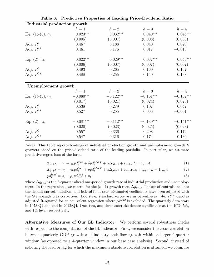
Table 6: Predictive Properties of Leading Price-Dividend Ratio

Industrial production growthh = 1 h = 2 h = 3 h = 4

Eq. (1)-(3), γh 0.023∗∗∗ 0.032∗∗∗ 0.040∗∗∗ 0.046∗∗∗

(0.005) (0.007) (0.008) (0.008)Adj. R2 0.467 0.188 0.040 0.020Adj. R2* 0.461 0.176 0.017 −0.013

Eq. (2), γh 0.022∗∗∗ 0.029∗∗∗ 0.037∗∗∗ 0.043∗∗∗

(0.006) (0.007) (0.007) (0.007)Adj. R2 0.493 0.265 0.169 0.167Adj. R2* 0.488 0.255 0.149 0.138

Unemployment growthh = 1 h = 2 h = 3 h = 4

Eq. (1)-(3), γh −0.080∗∗∗ −0.122∗∗∗ −0.151∗∗∗ −0.162∗∗∗

(0.017) (0.021) (0.024) (0.023)Adj. R2 0.538 0.279 0.107 0.047Adj. R2* 0.527 0.255 0.066 −0.001

Eq. (2), γh −0.081∗∗∗ −0.112∗∗∗ −0.139∗∗∗ −0.151∗∗∗

(0.020) (0.023) (0.025) (0.023)Adj. R2 0.557 0.336 0.208 0.172Adj. R2* 0.547 0.316 0.174 0.130

Notes: This table reports loadings of industrial production growth and unemployment growth hquarters ahead on the price-dividend ratio of the leading portfolio. In particular, we estimatepredictive regressions of the form:

∆gt+h = γ0 + γhpdleadt + δpdMKT

t + α∆gt−1 + εt+h, h = 1, .., 4 (1)

∆gt+h = γ0 + γhpdleadt + δpdMKT

t + α∆gt−1 + controls + εt+h, h = 1, .., 4 (2)

pdleadt = ρ0 + ρ1pdleadt−1 + ut (3)

where ∆gt+h is the h-quarter ahead one-period growth rate of industrial production and unemploy-ment. In the regressions, we control for the (t−1)-growth rate, ∆gt−1. The set of controls includesthe default spread, inflation, and federal fund rate. Estimated coefficients have been adjusted withthe Stambaugh bias correction. Bootstrap standard errors are in parentheses. Adj R2* denotesadjusted R-squared for an equivalent regression where pdlead is excluded. The quarterly data startin 1973:Q1 and end in 2012:Q4. One, two, and three asterisks denote significance at the 10%, 5%,and 1% level, respectively.

Alternative Measures of Our LL Indicator. We perform several robustness checks

with respect to the computation of the LL indicator. First, we consider the cross-correlation

between quarterly GDP growth and industry cash-flow growth within a larger 6-quarter

window (as opposed to a 4-quarter window in our base case analysis). Second, instead of

selecting the lead or lag for which the maximum absolute correlation is attained, we compute

13

Table 7: Robustness Checks±6 Lags Average LL x11 SAAR Granger Causality Granger Causality VW

LL LL Strong LL LL Strong LL LL Strong LL LL Strong LL LL StrongCAPM α 4.62∗∗ 5.07∗∗ 2.94∗ 3.25∗ 4.05∗∗ 4.91∗∗ 3.20∗ 4.97∗∗ 2.89∗ 5.25∗∗

(2.13) (2.41) (1.68) (1.73) (1.90) (2.00) (1.66) (2.52) (1.52) (2.22)FF3 α 3.03∗ 4.24∗ 2.95∗ 4.50∗∗∗ 3.97∗ 5.38∗∗ 3.56∗ 4.8 3.62∗ 5.59∗

(1.76) (2.43) (1.58) (1.56) (2.27) (2.36) (2.02) (3.17) (1.89) (2.86)Turnover 0.19 0.28 0.21 0.27 0.32 0.43 0.18 0.27 0.17 0.25

Notes: This table is based on real annualized value-weighted returns of portfolios of firms sorted according to their industry-level lead-lag (LL)indicator. Both the LL factor and the LL Strong factor are computed as in table 1. Turnover measures the percentage of industries entering orexiting from a portfolio. Return data are monthly over the sample 1972:01–2012:12. Industry definitions are from Kenneth French’s website.CAPM α (FF3 α) denotes average excess returns unexplained by the CAPM (Fama-French three-factor model). The numbers in parenthesesare standard errors adjusted according to Newey and West (1987). One, two, and three asterisks denote significance at the 10%, 5%, and1% levels, respectively. Results from the benchmark formation of the portfolios are reported in table 1. Here we depart from the benchmarkprocedure by (a) taking the maximum cross-correlation over a ±6-quarter horizon; (b) taking an average of the leads/lags over a ±4-quarterhorizon weighted by their cross-correlations in absolute values; (c) seasonally adjusting the industry cash flows using the BEA X11 procedureinstead of seasonal dummies; (d) using the Granger causality methodology to determine leads/lags instead of cross correlations; (e) determininglead/lags using Granger causality where lead and lags are weighted by their respective t-statistics.

14

an average lead-lag weighted by the absolute values of the cross-correlation coefficients.6 We

find that the average return of our LL portfolio still cannot be explained by the FF3 model.

These results suggest that our findings are not sensitive to the specific way in which we

assign a lead-lag indicator to an industry.

X11 Method. Aggregate data are adjusted for seasonality by applying the X11 method,

whereas our COMPUSTAT-based cash-flow measures are seasonally-adjusted using dummy

variables. Using the X11 method on industry-level cash flows does not alter our main results

in a significant way.

Granger causality. In a variation of our benchmark approach we construct a lead-lag

measure that employs the Granger causality to establish leads and lags between industry

cash-flow growth and GDP growth. In particular, we say that an industry is lagging GDP, if

GDP growth Granger-causes the cash-flow growth of this industry. In the opposite direction,

an industry leads GDP if the industry cash-flow growth Granger-causes GDP growth. In

the absence of any causality, we assign zero to the lead-lag measure. When both time series

Granger cause each other, we say that the lead-lag relation is undetermined and treat the

respective industry cash-flow as contemporaneous to GDP.

More specifically, we regress industry i’s cash-flows growth, ∆git, on a constant, its past

realization up to 4 lags, as well as past realizations of GDP growth, ∆gGDP :

∆git = c+4∑j=1

αj∆git−j +

4∑j=1

γj∆gGDPt−j + eit. (2)

We then test the hypothesis H0 : γ1 = γ2 = γ3 = γ4 = 0. If we fail to reject H0, we

argue that ∆gGDP Granger causes ∆gi, meaning that industry i lags GDP. We identify

the indicator value, that is, the corresponding lead, either by selecting the γj with highest

significance (based on the respective t-statistic), or by computing weighted average of all the

γj coefficients using their t-statistics as weights (Granger Causality VW). For the Granger

causality tests, we increase the rolling window to 40 quarters. We proceed in a similar

way when looking at leads.7 Our main results are robust to this alternative specification.

Furthermore, in Appendix A we show that our results continue to hold also when we consider

6In this case, the LL indicator is computed as∑4i=−4 i ·

|ρi|∑4i=−4 |ρi|

, where ρi = corr(∆GDPt,∆CFt+i).7In particular, for each industry we estimate the following equation:

∆gGDPt = c+

4∑j=1

αj∆gGDPt−j +

4∑j=1

γj∆git−j + eit (3)

If we fail to reject the null hypothesis, we conclude that cash-flow growth of industry i Granger causes theGDP growth and consequently industry i leads GDP.

15

aggregate consumption growth as opposed to GDP growth (see Table A3).

2.3 Cross Sectional Tests

Pricing tests. We use GMM to estimate the following linear pricing model

Rexi,t = ai + βi · Ft + ui,t (4)

E[Rexi,t ] = βiλ+ vi, (5)

in which Rex denotes excess returns, i indexes the test assets, and the β and λ coefficients

measure the exposure of returns to and the market price of risk of our factors, Ft, respectively.

Efficient standard errors are corrected for autocorrelation and heteroskedasticity following

Newey and West (1987).8 Our goal is to test whether our LL risk factor is priced in the cross

section of equity returns.

We first run an unconditional analysis with respect to the role of LL in the pricing of

industries. The purpose of this first step is to show that the LL-beta of an industry is closely

related to the value obtained for the LL indicator for this industry. This justifies that in the

ensuing conditional analysis individual stocks are sorted with respect to their conditional

betas for the LL factor.

Pricing industries. We start our analysis using portfolios based on 30 industries as test

assets. Table 8 provides some guidance on our estimated industry-level exposure to the LL

factor. Specifically, we focus on the three industries that most frequently enter the leading

and the lagging portfolios. For each industry, we show its returns loading on the LL factor

(βLL), its average market share, and descriptive statistics concerning its LL indicator.

First of all, we note that the exposure to the LL risk factor of the most frequently leading

firms are all positive, whereas the opposite is true for the three industries most frequently

included in the lagging portfolio. We consider this result as an important consistency check.

Second, in interpreting the numerical values of these exposures one has to keep in mind

that even the three most frequently leading or lagging industries are not always included in

the respective portfolio, implying that the unconditional measures that we report tend to

have moderate cross-sectional variation. As an example, in the 2007 recession Finance was

a leading industry, but historically it lagged GDP slightly.

In Table 9, we report our results for both the market prices of risk and the implied

stochastic discount factor loadings associated with our four factors. In each panel, the

top portion refers to our setting where portfolios ar formed from 30 industries (30-industry

8We use a two-step procedure. In the first iteration, we set the weighting matrix for the moment conditionsequal to the identity matrix. In the second iteration, we use the optimal weighting matrix from our firstiteration.

16

Table 8: Industry Exposures to the Lead-Lag Factor

Top 3 industries

βLL Market share,%LL Indicator

Mean MedianHealth 0.23 10.39 0.02 1.00Tobacco products 0.23 0.88 0.31 1.00Consumer goods 0.18 4.88 0.20 0.00

Bottom 3 industries

βLL Market share,%LL Indicator

Mean MedianBusiness equipment -0.26 11.64 -0.97 -1.00Finance -0.00 2.56 -0.55 -1.00Telecommunication -0.08 5.76 -0.29 -1.00

Notes: This table provides a summary of the first stage of our GMM estimation of the linear factormodel detailed in equations (4) and (5). The top (bottom) panel lists the top three industries mostfrequently included in our leading (lagging) portfolio. βLL represents the exposure of industryreturns to the LL risk factor. Market share is the average market value of the industry of interestdivided by total market capitalization over our sample (1972:01–2012:12). LL Indicator denotes thelead (when positive) or the lag (when negative) of industry cash-flow growth with respect to U.S.output growth. The indicator is computed in two steps. First, each quarter we compute the cross-correlation between industry-level output growth and domestic output growth for leads and lags ofup to four quarters each using a rolling window of 20 quarters. Second, we identify the lead or lagfor which the maximum absolute cross-correlation is attained and assign it to the correspondingindustry. A positive (negative) LL indicator denotes an industry whose output growth leads (lags)GDP growth.

portfolios). As in Cochrane (2005), we represent the discount factor as mt = m − bft, so

that

b = E(ftf′t)−1λ, (6)

where ft = [MKTt, SMBt, HMLt, LLt] is the the vector of factors. We find that both the

factor risk premium λLL and the pricing kernel loading bLL are statistically significant at the

10% level. Hence, these tests confirm that our LL factor is both relevant and required when

it comes to pricing the cross section of industry excess returns. These results are robust and

hold also when working with 38- and 49-industry portfolios.9 In Appendix A, we show that

these results are still significant, albeit at a higher significance level, when we add either

momentum or durability to set of risk factors (see Table A4).

Cross-sectional fit at the industry-level. In Figure 2, we depict the link between

the average excess returns predicted by our four-factor model (x-axis) and their realized

9Fama and French (1993) do not estimate market prices of risk as we do. We run the Fama-MacBethregressions replication code choosing our industry portfolios as test assets. In this cross section, we obtainedpoorly identified, and often negative, market price of risk for both SMB and HML.

17

Table 9: Prices of Risk and Pricing Kernel Loadings

E[Rexi ] = βMKTλMKT + βSMBλSMB + βHMLλHML + βLLλLL

λMKT λSMB λHML λLL30 industries

0.56∗∗∗ -0.14 -0.03 0.71∗

(0.21) (0.25) (0.23) (0.39)38 industries

0.56∗∗∗ -0.20 0.04 0.61∗

(0.20) (0.20) (0.26) (0.32)49 industries

0.58∗∗∗ -0.21 -0.09 0.67∗

(0.20) (0.23) (0.25) (0.41)

mt = m− bMKTMKTt − bSMBSMBt − bHMLHMLt − bLLLLtbMKT bSMB bHML bLL

30 industries0.04∗∗∗ -0.03 0.00 0.07∗∗

(0.01) (0.03) (0.03) (0.04)38 industries

0.04∗∗∗ -0.03 0.02 0.07∗∗

(0.01) (0.02) (0.03) (0.03)49 industries

0.04∗∗∗ -0.05∗ -0.01 0.08∗∗

(0.01) (0.03) (0.03) (0.04)

Notes: This table presents factor risk premia and the exposures of the pricing kernel to the FF3factors (MKT , SMB, HML) and our lead-lag factor (LL). We employ the generalized method ofmoments (GMM) to estimate the linear factor model stated in equations (4)–(5). Using a linearprojection of the stochastic discount factor m on the factors (m = m − f ′b), we determine thepricing kernel coefficients as b = E[ff ′]−1λ. Our sample consists of monthly returns for 30-, 38-and 49-industry portfolios from January 1972 through December 2012. The numbers in parenthesesare standard errors adjusted according to Newey and West (1987). One, two, and three asterisksdenote significance at the 10%, 5%, and 1% levels, respectively.

counterparts (y-axis) for the 30-industry portfolios. We obtain similar results also when

working with 38- and 49-industry portfolios (see Table A5 in the appendix).

The top (bottom) left panel shows the results for the CAPM (FF3) model. The corre-

sponding graphs on the right show how the results change when we add the LL factor to

the base models shown on the left. Given this representation, improvements in the model fit

imply combinations of predicted and realized average excess returns located closer to the 45-

degree line. A visual inspection of our graphs reveals that adding the LL factor substantially

improves the pricing quality.

More precisely, in each graph we explicitly label the ten industries with the highest pricing

errors in their respective models and report the associated mean-squared pricing errors. As

18

we turn our attention to the panels on the right, we can see that when the LL factor is

included, the predicted average excess returns of these industries move much closer to the

realized values. As a result, our factor does particularly well for those industries that can

be considered outliers in the CAPM and the FF3 model.

To quantify the additional pricing power of our LL factor, we show the overall mean

squared pricing error (MSE) as well as the average of the ten largest pricing errors (MSE10)

above each of the two graphs. Several observations are important here. First, adding SMB

and HML to the CAPM decreases the overall MSE from 4.14 to 2.60, whereas adding just

LL reduces the average squared pricing error to 2.01, i.e., MSE declines by more than 50

percent.10 The effect is even more pronounced for the industries with ten largest CAPM

pricing errors: adding LL to the CAPM reduces MSE10 by about 60 percent.

The effect of introducing LL remains strong also with respect to the FF3 model. Adding

our factor to the FF3 model reduces overall average squared pricing errors by about one

third (from 2.60 to 1.73). For the ten industries with the largest pricing errors, the gain in

pricing quality is slightly larger, in the order of 40% (with pricing errors declining from 6.46

to 3.67). Overall, these numbers provide additional evidence that the timing of risk is priced

in the cross section of industry returns.

Portfolios sorted on firm-level LL-exposure. Our analysis shows that there is a pos-

itive link between the exposure of the returns of leading industries to the LL factor and the

LL indicator. Here we take this link seriously and use the firm-level exposure to the LL

factor to proxy the extent to which a firm leads/lags the cycle.

Specifically, we start by taking our LL factor from our benchmark procedure that considers

30 industries. For each firm, we then compute its conditional exposure to the LL factor

(βLL,i,t) over a rolling-window that includes the past 60 months. We control for the FF3

factors in the regression and sort firms according to their βLL,i,t into 30 portfolios that we

use as test assets. By grouping together all firms with strongly positive (negative) exposure,

this procedure bundles the most leading (lagging) firms in the economy across industries.

These portfolios are re-formed once a year.

Our results are reported in Table 10 (top portion of each panel) and confirm what we

had found in our analysis with industries: the LL factor is priced and it enters the discount

factor in an independent and significant way.

We then turn our attention to firm heterogeneity within industries. We focus on 38 (49)

industries and sort firms within each industry in 3 (2) portfolios according to their βLL,i,t

exposure.11 This procedure enables us to have a larger cross section of test assets and

10The root-mean-squared error (RMSE) can be obtained as follows: RMSE = 12 ·√MSE/100. For the

CAPM, for example, this value is 2.44.11When we compute the βLL,i,t with 38 (49) industries we also use the benchmark LL factor that we

obtained working with 30 industries.

19

4 6 8 10 12

4

6

8

10

12

Predicted expected excess returns

Mea

n ex

cess

ret

urn

FoodBeer

Smoke

Oil

Util

Steel

FabPr

Autos

BusEq

Other

MKT factor, MSE = 4.14, MSE10

= 10.71

4 6 8 10 12

4

6

8

10

12

Predicted expected excess returns

Mea

n ex

cess

ret

urn

FoodBeer

Smoke

Oil

Util

Steel

FabPr

Autos

BusEq

Other

MKT and LL factors, MSE = 2.01, MSE10

= 4.00

4 6 8 10 12

4

6

8

10

12

Predicted expected excess returns

Mea

n ex

cess

ret

urn

Beer

Smoke

Clths

Mines

Coal

HshldSteelAutos

Fin

Other

FF3 factors, MSE = 2.60, MSE10

= 6.46

4 6 8 10 12

4

6

8

10

12

Predicted expected excess returns

Mea

n ex

cess

ret

urn

Beer

Smoke

Clths

Mines

Coal

HshldSteelAutos

Fin

Other

FF3 and LL factors, MSE = 1.73, MSE10

= 3.67

Fig. 2: Predicted vs. Realized Average Excess Returns for 30 Industries

This figure presents realized average excess returns (y-axis) for 30-industry portfolios plotted against

the predicted mean excess returns from linear factor models (x-axis). Monthly returns are mul-

tiplied by 1200. We compare the performance of the CAPM and FF3 models with and without

the addition of our lead-lag factor (LL). In the top two panels, we highlight 10 industries: the top

5 with a positive deviation from the 45-degree line, and the top 5 with a negative deviation. In

the bottom two panels, we select the 10 industries in a similar way, but with respect to the FF3

model. MSE and MSE10 stand for mean squared error and are computed using all the 30-industry

portfolios and the 10-industry portfolios with the largest absolute pricing errors, respectively. The

MSE is computed in percent monthly returns and multiplied by 100.

confirms that the LL factor is still priced in the cross-section and represents a significant

component of the discount rate.

3 A Rational Explanation of the Leading Premium

Intuition based on no-arbitrage. Consider two stocks, denoted as leading and lagging.

For the sake of simplicity, assume that they both pay dividends only once, n periods from

now. From a time-0 perspective, the dividend of the leading firm, Dleadn , is assumed to

20

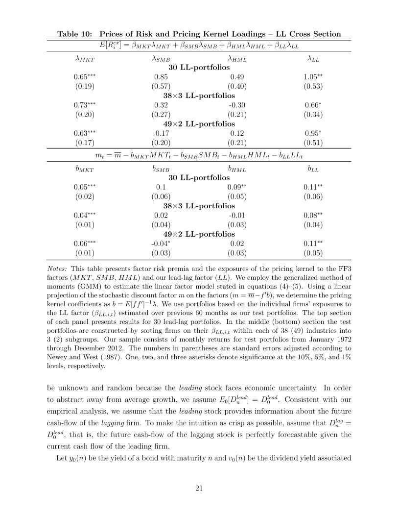
Table 10: Prices of Risk and Pricing Kernel Loadings – LL Cross Section

E[Rexi ] = βMKTλMKT + βSMBλSMB + βHMLλHML + βLLλLL

λMKT λSMB λHML λLL30 LL-portfolios

0.65∗∗∗ 0.85 0.49 1.05∗∗

(0.19) (0.57) (0.40) (0.53)38×3 LL-portfolios

0.73∗∗∗ 0.32 -0.30 0.66∗

(0.20) (0.27) (0.21) (0.34)49×2 LL-portfolios

0.63∗∗∗ -0.17 0.12 0.95∗

(0.17) (0.20) (0.21) (0.51)

mt = m− bMKTMKTt − bSMBSMBt − bHMLHMLt − bLLLLtbMKT bSMB bHML bLL

30 LL-portfolios0.05∗∗∗ 0.1 0.09∗∗ 0.11∗∗

(0.02) (0.06) (0.05) (0.06)38×3 LL-portfolios

0.04∗∗∗ 0.02 -0.01 0.08∗∗

(0.01) (0.04) (0.03) (0.04)49×2 LL-portfolios

0.06∗∗∗ -0.04∗ 0.02 0.11∗∗

(0.01) (0.03) (0.03) (0.05)

Notes: This table presents factor risk premia and the exposures of the pricing kernel to the FF3factors (MKT , SMB, HML) and our lead-lag factor (LL). We employ the generalized method ofmoments (GMM) to estimate the linear factor model stated in equations (4)–(5). Using a linearprojection of the stochastic discount factor m on the factors (m = m−f ′b), we determine the pricingkernel coefficients as b = E[ff ′]−1λ. We use portfolios based on the individual firms’ exposures tothe LL factor (βLL,i,t) estimated over previous 60 months as our test portfolios. The top sectionof each panel presents results for 30 lead-lag portfolios. In the middle (bottom) section the testportfolios are constructed by sorting firms on their βLL,i,t within each of 38 (49) industries into3 (2) subgroups. Our sample consists of monthly returns for test portfolios from January 1972through December 2012. The numbers in parentheses are standard errors adjusted according toNewey and West (1987). One, two, and three asterisks denote significance at the 10%, 5%, and 1%levels, respectively.

be unknown and random because the leading stock faces economic uncertainty. In order

to abstract away from average growth, we assume E0[Dleadn ] = Dlead

0 . Consistent with our

empirical analysis, we assume that the leading stock provides information about the future

cash-flow of the lagging firm. To make the intuition as crisp as possible, assume that Dlagn =

Dlead0 , that is, the future cash-flow of the lagging stock is perfectly forecastable given the

current cash flow of the leading firm.

Let y0(n) be the yield of a bond with maturity n and v0(n) be the dividend yield associated

21

with the cash-flow Dleadn . Furthermore, assume for simplicity Dlead

0 = Dlag0 ≡ D0. By no

arbitrage, the dividend yield for the lagging firm must be equal to y0(n), since its cash-flow

is known at time 0, so that P lag0 = D0e

−y0(n)n. In contrast, the leading firm must offer a

yield of v0(n), i.e., P lead0 = D0e

−v0(n)n. This implies that the following holds:

P lag0

D0

/P lead

0

D0

=pdlag0

pdlead0

= e(v0(n)−y0(n))n

=E0[Dlead

n ]

F0,n

,

where F0,n is the future (or forward) price at time 0 for the dividend Dleadn to be paid at

time n, and pdi0 is the price-dividend ratio of claim i at time 0. This implies

1

n

(log pdlag0 − log pdlead0

)= v0(n)− y0(n),

i.e., the difference between the log valuation ratios of the lagging and the leading stock is

equal to the forward equity premium (in the terminology of Binsbergen et al. (2012)) for a

maturity of n periods.

If investors are adverse to dividend uncertainty, we have F0,n < E0[Dleadn ], and lagging

firms are more valuable than leading firms. Equivalently, an investment strategy long in the

leading and short in the lagging stock should pay the forward equity premium on leading

dividends.

This result is important for two reasons. First, the forward equity premium features no

time-discounting, as it is determined by the difference between the expected dividend at

time n and the certain payoff F0,n paid at time n, i.e., it can be regarded as the price of a

static lottery. Hence this premium is a pure measure of the value of advance information on

n-period ahead cash-flows.

Second, the forward equity premium equals the difference between equity and bond yields

of the same maturity. Thus to obtain a positive leading premium we need a model that

produces a significant positive gap between the yield curve of zero-coupon equities and that

of bonds over the horizon for which leading industry cash-flows predict lagging industry cash

flows.

It is important to highlight that the existence of a leading premium depends on the spread

between the equity and the bond yield curve, not on the slope of the equity curve. In what

follows, we adopt an equilibrium model that delivers an upward sloping aggregate equity

yield curve for the sole sake of analytical tractability. Richer settings like those of Lettau

and Wachter (2007), Lettau and Wachter (2011), Croce et al. (2014), and Ai et al. (2017),

which are consistent with the empirical evidence in Binsbergen et al. (2012), Binsbergen

22

et al. (2013), and Binsbergen and Koijen (2017), would produce similar insights about the

nature of the leading premium.

An equilibrium model. We provide a rational explanation of our leading premium in

an equilibrium model featuring two main elements: (a) an information structure affected by

leads and lags of cash flows; and (b) preferences sensitive to the timing of information about

future growth. Specifically, we assume that the representative agent has Epstein and Zin

(1989) preferences, i.e.,

Ut =

[(1− δ)C

1− 1ψ

t + δEt[U1−γt+1

] 1− 1ψ

1−γ

] 1

1− 1ψ

and her stochastic discount factor is

Mt = δe−1ψ

∆ct

(Ut

Et−1[U1−γt ]

11−γ

)1/ψ−γ

.

In this economy, there are three fundamental cash flows: consumption, C; a redundant

cash flow that provides anticipated information, Dlead; and a lagged redundant cash flow,

Dlag. We assume that the following holds:

∆ct+1 = µ+ xt−jc + εct+1 (7)

xt+1 = ρxt + εxt+1 (8)

∆dleadt+1 = µ+ φleadx xt + φlead0 εc,t+1 + εd,leadt+1 (9)

∆dlagt+1 = µ+ φlagx xt−jd +

jlag∑f=0

φlagf εc,t+1−f + εd,lagt+1 , (10)

where

vt+1 =

εct+1

εxt+1

εd,leadt+1

εd,lagt+1

∼ N .i .i .d .(0,Σ), and Σ = diag(σ2c , σ

2x, σ

2d,lead, σ

2d,lag).

According to this law of motion, the leading portfolio has predictive power for expected

consumption growth jc periods ahead, that is, Et[∆ct+1+jc ] = xt. For the lagged cash flows,

the time lag on the long-run component is denoted by jd. We also allow the agent to

have advance information with respect to the exposure of the lagged cash flow to short-run

consumption shocks over a maximum time horizon of jlag periods. We do this to be consistent

with the data, but it is not the main driver of our results.

23

The endogenous returns associated with this log-linear setting are reported in Appendix

C. In what follows, we focus on the procedure that we use to calibrate these portfolio cash

flows.

Calibration Strategy. Quarterly consumption data are from the BEA and include non-

durables and services. To identify xt−jc , we run a standard forecasting regression using the

thirteen factors formed by Jurado et al. (2015) and represent the estimated long-run risk

component as an AR(1) process, consistent with equation (8).12 This procedure enables us

to identify both long-run (εx,t) and short-run (εc,t) consumption news.

We compute the dividends paid out by both our lead and lag portfolios and aggregate

them to a quarterly frequency.13 We deflate them using quarterly US CPI and then regress

these cash flows on leads and lags of both short- and long-run consumption news, consistent

with equations (9)–(10). We use adjusted R2 to optimally pin down the maximum num-

ber of leading/lagging periods, as detailed in Appendix B. We set statistically insignificant

coefficients to zero.

We summarize our main results in Table 11. The consumption long-run component lags

that of the leading cash flow by 27 quarters (jc = 81 months). The long-run component of

the cash flow of the lagged portfolio lags by 47 quarters (jd = 141 months). To be consistent

with the data, we also allow this cash flow to load on lagged short-run consumption shocks.

According to our results, anticipated information on these shocks plays a very marginal role

(the estimated φlagf coefficients can be found in Table B1 in the appendix).

The data suggest that the dividends of the leading portfolio tend to be more exposed to

long-run growth news than those of the lagged portfolio. Consistent with these results, we set

φleadx = 8.60 and φlagx = 6.39. The relevance of this observation is twofold. First, we properly

control for heterogeneous exposure to shocks, as suggested by Bansal et al. (2005). Second,

after accounting for heterogeneity in exposure we can isolate the role of heterogeneity in the

timing of exposure.

The properties of aggregate consumption growth are consistent with both prior findings

and our own estimation results. We set the monthly persistence of long-run risk to 0.9, a value

12The point estimate of ρ is corrected for the small-sample bias (Kendall (1954)):

E (ρ− ρ) = − (1 + 3ρ)

n.

13Let Rexp,t and Rcump,t represent the ex- and cum-dividend returns of portfolio p. Let Vp,t be the ex-dividendvalue of the investment strategy in portfolio p at time t. Dividends Dp,t are then computed recursively:

Dp,t = Vp,t−1(Rcump,t −Rexp,t)Vp,t = Vp,t−1R

exp,t,

assuming Vp,0 = 1.

24

lower than that in Bansal and Yaron (2004) and consistent with our empirical confidence

interval.14 The volatility of the long-run news, σx, is calibrated to be consistent with the R2

that we obtain from estimating equation (7). The volatility of the consumption short-run

shock is calibrated to a low level, consistent with the fact that we use post-1972 data, i.e.,

observations from a period of great moderation.

Results. Under our benchmark calibration, we set the preference parameters as in Bansal

and Yaron (2004). Specifically, the relative risk aversion (γ) is set to 10; the intertemporal

elasticity of substitution (ψ) is 1.5; and the subjective discount rate (δ) is set to 0.99 to keep

the risk-free rate to a low level.

Our benchmark model produces an annualized LL premium of 3.10%, a number consis-

tent with our empirical evidence. Furthermore, when we remove advance information by

setting jc = jd = 0, this premium declines to 1.65%. That is, advance information alone is

responsible half of the model-implied LL premium. The remaining portion of the premium

is driven by heterogeneous exposure to the long-run component (φleadx > φlagx ).

These results are mostly driven by information about long-run growth, as can be seen by

comparing our benchmark setting with the case in which we remove short-run risk exposure

from the cash flow of both the leading and the lagging portfolios (φpf = 0 for all f and

p ∈ lead, lag). In this case, our results are actually enhanced, as the LL premium is even

closer to its empirical counterpart.

We also compute the utility-consumption ratio associated with these scenarios. By com-

paring these ratios in log units, we can compute welfare benefits in terms of percentage

of lifetime consumption. Specifically, we find that advance information about the long-run

component of growth in the economy produces welfare benefits in the order of just 6% of

lifetime consumption.

In order to correctly interpret this figure, we run the Lucas (1987) experiment in our

economy and obtain welfare benefits of removing all uncertainty in the order of 65%.15 As a

result, the advance information that we identify in the cross section of industries represents

less than 10% of the maximum attainable welfare benefits.

Epstein et al. (2014) point out that in the Bansal and Yaron (2004) model, most of the

Lucas welfare benefits originate from full resolution of uncertainty, not from the removal of

deterministic fluctuations. Our computations show that the early resolution of uncertainty

in the cross section of industries is simultaneously valuable but limited, as it carries a strong

market price of risk, but reveals future long-run consumption dynamics over a relatively

short horizon.

14We estimate the quarterly persistence parameter ρ and report the inference for ρ1/3. Standard errorsare computed using the delta method.

15This number is much smaller than that in Croce (2013), as our consumption process is calibratedaccording to post-1972 data, i.e., its volatility is moderate.

25

Table 11: Predictions for Quantities and Prices

Panel A: Benchmark Calibration

δ12 γ ψ 12µ σc√

12 V (x)/V (∆c) ρ φleadx φlagx jc jd0.99 10 1.50 1.80% 0.65% 0.57% 0.90 8.60 6.39 81 141

Data 0.65% 0.50% 0.83 8.60 6.39 81 141s.e. (0.02) (0.04) (3.86) (4.71)

Panel B: Main MomentsEZ case (ψ = 1.5) CRRA (ψ = γ−1 = 0.1)

Bench- No lead LRR only Bench- No lead LRR onlyDATA mark (jc = jd = 0) (φpf = 0, ∀f) mark (jc = jd = 0) (φpf = 0, ∀f)

E[rex,leadd − rex,lagd ] 4.04 (0.60) 3.09 1.66 3.48 0.04 0.03 0.00

E[rex,leadd ] 9.00 (0.72) 7.64 7.84 7.37 0.28 0.28 0.00

E[rex,lagd ] 4.96 (0.89) 4.56 6.19 3.89 0.24 0.24 0.00

σ[rex,leadd ] 16.79 (0.54) 26.83 26.24 26.50 17.08 9.08 16.46

σ[rex,lagd ] 18.85 (0.60) 22.03 25.00 19.20 15.74 17.60 15.34E[rf ] 0.94 (0.12) 2.24 2.22 2.24 19.01 19.01 19.01E[rexc ] - 0.33 0.36 0.33 −0.30 −3.45 −0.30σ[rexc ] - 1.22 1.26 1.22 8.26 26.41 8.26

U/C - 3.99 3.76 3.99 1.34 1.31 1.34

Notes: Panel A summarizes the benchmark monthly calibration of the cash-flow dynamics described in equations (7)–(10). The entries for thedata are obtained from formal estimation procedures applied to quarterly consumption and dividend data. The long-run risk volatility σx isselected to align the V (xt)/V (∆c) ratio in the model to the R2 of our regressions in the data. For the leading portfolio, the annualized volatilityof the dividend-specific shocks is set to 7%. For the lagged portfolio we use a figure twice as large, consistent with our estimation results. Theexposures to short-run shocks are set as in appendix table B1. In panel B, we report key annualized moments in percentage terms. When weset jc = jd = 0, we remove all advance information about the long-run growth component in the economy. The column labeled ‘LRR Only’features advance information about the long-run component, but it removes exposure of dividends to short-run consumption risk at all horizons(φpf = 0,∀f, p ∈ lead, lag). The rightmost three columns refer to the case in which we adopt CRRA preferences (ψ = γ−1). U/C denotes theaverage utility-consumption ratio. All standard errors are Newey-West adjusted.

26

Table 12: Short-Run Risk Exposure (Simplified)

φlead0 φlag0

6.58∗ −6.12(3.54) (5.05)

Notes: This table presents estimated loadings of the leading and lagging dividends on the contem-poraneous shock to the consumption growth, as specified in the system of equations (7)–(10). Theestimation is restricted by imposing that φif = 0, ∀f > 1, i.e., there is no anticipated informationwith respect to short-run consumption news. Numbers in parentheses are Newey-West adjustedstandard errors.

We also look at the aforementioned model configurations under the special case of time-

additive preferences, i.e., when ψ = 1γ

= 0.1. Since in this case the representative agent does

not care about the timing of resolution of uncertainty, advance information is not priced. As

a result, the lead-lag expected return difference disappears, and our empirical findings take

the form of an anomaly. In Appendix C, the reader can find explicit derivations of the LL

premium in the context of simple lead-lag structures.

Link to our multifactor model. In order to investigate our model’s ability to reproduce

the cross-sectional pricing predictions found in the data, we construct a synthetic cross

section of redundant dividend claims that differ in their exposure to fundamental shocks and

in the timing of their exposure.

Specifically, we let the dividends for cash flow i follow the dynamics specified in equation

(10) with specific parameters jid, φif , . . . . Since the effect of current and past short-run shocks

on risk premiums is modest, we focus only on exposure to contemporaneous short-run shocks,

i.e., we set φif = 0 for all f > 1. For consistency, we re-estimate the system of equations

(9)–(10) and report the new estimates in Table 12. We omit the long-run risk exposures

φleadx and φlagx , because they remain unaffected.

Our simulated cross section of cash flows consists of (a) a leading dividend claim which

depends on xt; (b) a lagging asset that lags the leading claim by 141 months, i.e, it depends

on xt−141; and (c) fifteen additional lagging claims with specific lags jid evenly spread out

between 0 and 141 months. Thus, some assets lead aggregate consumption (those with a

lagging period shorter than 81 months), whereas all other assets lag, as in the data.

Additionally, our synthetic assets differ in both their exposure to the long-run shock (φix)

and their exposure to the short-run shock (φif ). For the sake of consistency with the data, we

also allow these cash flows to randomly differ in their idiosyncratic volatility (σid, i = 1, .., 15).

This dimension is not crucial for our results.

For each synthetic asset, we uniformly draw a triplet (φix, φif , σ

id) from our estimated

intervals. For example, the interval for the φif values is consistent with the results in Table

12. Since we draw these parameters independently from jid, we are able to simulate a cross

27

section of returns in which heterogeneous exposure and heterogeneous timing of exposure to

shocks are distinct phenomena.

We use many repetitions of small samples of simulated returns. In each sample, we

construct the model-implied LL factor by computing the difference between leading and

lagging claim returns, as in the data. We proxy the market factor (MKT ) by focusing on

the return of the claim to aggregate consumption. We then estimate the following linear

factor models:E[Rex

i ] = βi,MKTλMKT + vi,

E[Rexi ] = βi,LLλLL + vi,

E[Rexi ] = βi,MKTλMKT + βi,LLλLL + vi,

(11)

where Rexi is mean excess return on a synthetic asset. For each sample, we compute the

mean squared error (MSE) between simulated returns and returns predicted by these three

different factor-based models. We depict the implied distribution of MSEs across simulated

samples in Figure 3 along with the point estimates obtained from our empirical investigation.

We highlight two important takeaways from this exercise. First, the cross section of our

synthetic returns can be explained by a two-factor linear model, where the market factor

picks up differences in exposure to risks, whereas the LL factor picks up heterogeneity in

the timing of exposure. For this reason, the LL factor systematically improves the MSE

by lowering its average and, more generally, by shifting more probability mass toward lower

MSE values.

Second, under our benchmark calibration the model fit improvement

MFI = 1−√

MSE(MKT + LL)/MSE(MKT ),

i.e., the relative improvement in MSE obtained by adding the LL factor, tends to be mod-

est compared to its empirical counterpart. According to our simulations, the probability of

observing our estimated MFI or a higher value is just 2%. The reason for this outcome

is related to the fact that volatilities are calibrated to modest values under the benchmark

calibration, and hence we do not have a sizeable heterogeneity across our relevant factors.

When we refine our calibration and increase our volatility parameters so that the volatility

of consumption growth is 2%, the improvement of fit associated with the LL factor becomes

more sizeable and our empirical estimate corresponds to the 70th percentile of our simu-

lated distribution. We find this result reassuring: under a refined calibration consistent

with long-sample US consumption variance, our model performs well both qualitatively and

quantitatively.

Further simulations results. Given our simulated cross section of cash-flows, we can

now investigate the properties of our empirical approach based on cross-correlograms to pin

28

0 0.05 0.1 0.150

10

20

30

40

50

60

70

80

MSE

MS

E d

istr

ibut

ion

Benchmark calibration

MKT factorLL factorMKT and LL factors

0 0.05 0.1 0.150

10

20

30

40

50

60

70

80

MSE

Refined calibration

MKT factorLL factorMKT and LL factors

0 0.2 0.4 0.6 0.80

5

10

15

Dis

trib

utio

n of

mod

el fi

t im

prov

emen

t

Model fit improvement (MFI)0 0.2 0.4 0.6 0.8

0

5

10

15

Model fit improvement (MFI)

E(MSE) = 1.59%

E(MSE) = 1.86%

E(MSE) = 3.10%

E(MSE) = 1.59%

Pr(MFI>30.47%) = 0.02 Pr(MFI>30.47%) = 0.32

Fig. 3: Mean Squared Error (MSE) Distribution

This figure examines the goodness of fit of the factor models described in the system of equations(11). The entries from the model are obtained from repetitions of small samples. The entries fromthe data are obtained from our estimates derived from post-1972 quarterly data. In the model,we construct a cross section of synthetic assets whose cash flows lag to different extents the cashflow of the leading claim. Assets also randomly differ in their exposure to short- and long-runrisk, as in the data. The LL factor is constructed as a spread in the returns of the most-leadingand most-lagging portfolios. In the model, the market return is proxied by the consumption claimreturn. In the top panels, we depict the MSEs across simulated samples. In the bottom panels,we depict the empirical distribution of the model fit improvement (MFI) obtained by adding theLL factor to the MKT factor (MFI = 1−

√MSE(MKT + LL)/MSE(MKT )). The point estimate

of MSE improvement in the data (using 30-industry portfolio returns) is represented by a verticaldashed line. The right panels are obtained using a refined calibration in which the total volatilityof consumption growth is set to its 1929–2008 estimate of 2%.

down the LL indicator. Our main results are reported in Table 13. The first column confirms

that when the model cash flows are all coincidental (jc = jd = 0), our procedure produces

no leading premium. Thus concerns about spurious results are mitigated.

When we instead have a proper lead/lag structure, our benchmark empirical procedure

captures a positive and significant leading premium. Not surprisingly, the magnitude of the

premium measured in the data is much smaller than the maximum spread implied by the

29

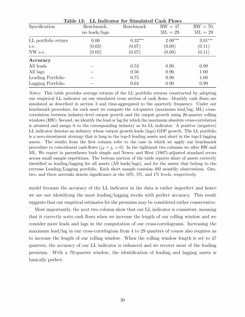
Table 13: LL Indicator for Simulated Cash FlowsSpecification Benchmark, Benchmark RW = 47 RW = 70,

no leads/lags ML = 29 ML = 29

LL portfolio return 0.00 0.32∗∗∗ 2.00∗∗∗ 3.01∗∗∗

s.e. (0.03) (0.07) (0.08) (0.11)NW s.e. (0.02) (0.07) (0.08) (0.11)

AccuracyAll leads − 0.53 0.90 0.99All lags − 0.56 0.96 1.00Leading Portfolio − 0.75 0.98 1.00Lagging Portfolio − 0.64 0.90 0.99

Notes: This table provides average returns of the LL portfolio returns constructed by adoptingour empirical LL indicator on our simulated cross section of cash flows. Monthly cash flows aresimulated as described in section 3 and time-aggregated to the quarterly frequency. Under ourbenchmark procedure, for each asset we compute the ±4-quarter (maximum lead/lag, ML) cross-correlation between industry-level output growth and the output growth using 20-quarter rollingwindows (RW). Second, we identify the lead or lag for which the maximum absolute cross-correlationis attained and assign it to the corresponding industry as its LL indicator. A positive (negative)LL indicator denotes an industry whose output growth leads (lags) GDP growth. The LL portfoliois a zero-investment strategy that is long in the top-3 leading assets and short in the top-3 laggingassets. The results from the first column refer to the case in which we apply our benchmarkprocedure to coincidental cash-flows (jd = jc = 0). In the rightmost two columns we alter RW andML. We report in parentheses both simple and Newey and West (1987)-adjusted standard errorsacross small sample repetitions. The bottom portion of the table reports share of assets correctlyidentified as leading/lagging for all assets (All leads/lags), and for the assets that belong to theextreme Leading/Lagging portfolio. Each short sample contains 492 monthly observations. One,two, and three asterisks denote significance at the 10%, 5%, and 1% levels, respectively.

model because the accuracy of the LL indicator in the data is rather imperfect and hence

we are not identifying the most leading/lagging stocks with perfect accuracy. This result

suggests that our empirical estimates for the premium may be considered rather conservative.

Most importantly, the next two column show that our LL indicator is consistent, meaning

that it correctly sorts cash flows when we increase the length of our rolling window and we

consider more leads and lags in the computation of our cross-correlograms. Increasing the

maximum lead/lag in our cross-correlogram from 4 to 29 quarters of course also requires us

to increase the length of our rolling window. When the rolling window length is set to 47

quarters, the accuracy of our LL indicator is enhanced and we recover most of the leading

premium. With a 70-quarter window, the identification of leading and lagging assets is

basically perfect.

30

4 Conclusion

In this study, we compute conditional leading/lagging indices for industry-level cash flows

with respect to US GDP. We find that leading industries, i.e., industries whose cash flows

contain information relevant for future aggregate growth, exhibit average returns that are

approximately 4% higher than those of lagging industries. This return difference remains

sizeable and significant even after adjusting for a large number of other risk factors.

We construct a novel factor, denoted as LL, by considering the returns on a zero-cost

portfolio long in leading and short in lagging firms. Our LL factor is priced in the cross

section of industry portfolio returns, and it has a significant loading in a model with a linear

stochastic discount factor in which the FF3 factors are included as well.

Our investigation implies at least two novel insights: (a) the cross section of industry

returns can be significantly explained by heterogeneity in the timing of exposure to shocks;

and (b) asset prices are sensitive to the timing of economic fluctuations.

We provide a theoretical foundation for our findings in the context of a rational equilibrium

model in which agents have a preference for early resolution of uncertainty and hence price

advance information about future cash flows. Our setting explains our empirical findings

and suggests that advance information in the cross section of industry cash flows is valuable

but limited, as it results in moderate welfare benefits.

Future work should extend our investigation by including other potentially valuable

sources of anticipated information. This task could be accomplished either by considering

other classes of financial securities, such as bonds and options, or by examining international

markets. A richer set of preferences could also be examined, including those in Caplin and

Leahy (2001).

31

References

Acharya, V., H. Almeida, F. Ippolito, and A. Perez. 2014. Credit lines as monitored liquidity

insurance: Theory and evidence. Journal of Financial Economics 112(3):287 – 319.

Ai, H. Information quality and long-run risks: Asset pricing and welfare implications. Unpublished

2007.

Ai, H., and R. Bansal. Risk Preferences and the Macroeconomic Announcement Premium. NBER

working paper 2016.

Ai, H., M. M. Croce, A. Diercks, and K. Li. 2017. News shocks and the production-based term

structure of equity returns. Review of Financial Studies. Forthcoming.

Albuquerque, R., and J. Miao. 2014. Advance information and asset prices. Journal of Economic

Theory 149:236–275.

Asness, C., A. Frazzini, and L. Pedersen. 2014. Low-risk investing without industry bets. Financial

Analysts Journal 70(1):24–41.

Bansal, R., and A. Yaron. 2004. Risks for the long run: A potential resolution of asset pricing

puzzles. Journal of Finance 59(4):1481–1509.

Bansal, R., R. F. Dittmar, and C. T. Lundblad. 2005. Consumption, dividends, and the cross

section of equity returns. Journal of Finance 60(4):1639–1672.

Belo, F., P. Colin-Dufresne, and R. Goldstein. 2014. Dividend dynamics and the term structure of

dividend strips. The Journal of Finance 70(3).

Binsbergen, J., and R. S. Koijen. 2017. The term structure of returns: facts and theory. Journal

of Financial Economics 124(1):1–21.

Binsbergen, J., M. W. Brandt, and R. S. Koijen. 2012. On the timing and pricing of dividends.

American Economic Review 102(4):1596–618.

Binsbergen, J., W. H. Hueskes, R. S. Koijen, and E. B. Vrugt. 2013. Equity yields. Journal of

Financial Economics 110(3):503–19.

Campbell, J. Y., and R. J. Shiller. 1988. Stock prices, earnings, and expected dividends. Journal

of Finance 43(3):661–676.

Caplin, A., and J. Leahy. 1993. Sectoral shocks, learning, and aggregate fluctuations. Review of

Economic Studies 60(4):777–794.

Caplin, A., and J. Leahy. 1994. Business as usual, market crashes, and wisdom after the fact.

American Economic Review 84(3):548–565.

32

Caplin, A., and J. Leahy. 2001. Psychological expected utility theory and anticipatory feelings.

Quarterly Journal of Economics 116(1):55–79.

Carhart, M. M. 1997. On persistence in mutual fund performance. Journal of Finance 52(1):57–82.

Cochrane, J. H. Asset Pricing – Revised Edition. Princeton University Press Princeton, NJ 2005.

Cochrane, J. H., and M. Piazzesi. 2005. Bond risk premia. American Economic Review 95(1):

138–160.

Croce, M. M. Welfare costs in the long run. Working Paper 2013.

Croce, M. M., M. Lettau, and S. C. Ludvigson. 2014. Investor information, long-run risk, and the

duration of risky cash-flows. Review of Financial Studies 28(3):706–742.

Epstein, L. G., and S. E. Zin. 1989. Substitution, Risk Aversion, and the Temporal Behavior of

Consumption and Asset Returns: A Theoretical Framework. Econometrica 57(4):937–69.

Epstein, L. G., Farhi, Emmanuel, and T. Strzalecki. 2014. How much would you pay to resolve

long-run risk? American Economic Review 104(9):2680–97.

Estrella, A., and F. S. Mishkin. 1998. Predicting us recessions: Financial variables as leading

indicators. Review of Economics and Statistics 80(1):45–61.

Fama, E. F., and K. R. French. 1993. Common risk factors in the returns on stocks and bonds.

Journal of Financial Economics 33(1):3–56.

Fama, E. F., and K. R. French. 1997. Industry costs of equity. Journal of Financial Economics 43

(2):153–193.

Fama, E. F., and K. R. French. 2012. Size, value, and momentum in international stock returns.

Journal of Financial Economics 105(3):457–472.

Fama, E. F., and K. R. French. 2015. A five-factor asset pricing model. Journal of Financial

Economics 116(1):1–22.

Gofman, M., G. Segal, and Y. Wu. Production networks and stock returns: The role of creative

destruction. Working Paper 2017.

Gomes, J. F., L. Kogan, and M. Yogo. 2009. Durability of output and expected stock returns.

Journal of Political Economy 117(5):941–986.

Gomme, P., F. E. Kydland, and P. Rupert. 2001. Home production meets time to build. Journal

of Political Economy 109(5):1115–1131.

Greenwood, J., and Z. Hercowitz. 1991. The allocation of capital and time over the business cycle.

Journal of Political Economy 99(6):1188–1214.

33

Hong, H., W. Torous, and R. Valkanov. 2007. Do industries lead stock markets? Journal of

Financial Economics 83(2):367–396.

Hou, K., C. Xue, and L. Zhang. 2015a. Digesting anomalies: An investment approach. Review of

Financial Studies 28(3):650–705.

Hou, K., C. Xue, and L. Zhang. A comparison of new factor models. Working Paper 2015b.

Jurado, K., S. C. Ludvigson, and S. Ng. 2015. Measuring uncertainty. American Economic Review

105(3):1177–1216.

Kadan, O., and A. Manela. Estimating the value of information. Working Paper 2016.

Kendall, M. 1954. Note on bias in the estimation of autocorrelation. Biometrika 41(3-4):403–404.

Kogan, L., and D. Papanikolaou. 2014. Growth opportunities, technology shocks, and asset prices.

Journal of Finance 69(2):675–718.

Koijen, R. S., H. Lustig, and S. Van Nieuwerburgh. 2017. The cross-section and time series of

stock and bond returns. Journal of Monetary Economics 88:50–69.

Lettau, M., and J. A. Wachter. 2007. Why Is Long-Horizon Equity Less Risky? A Duration-Based

Explanation of the Value Premium. Journal of Finance 62(1):55–92.

Lettau, M., and J. A. Wachter. 2011. The Term Structure of Equity and Interest Rates. Journal

of Financial Economics 101(1):90–113.

Lettau, M., M. Maggiori, and M. Weber. 2014. Conditional risk premia in currency markets and

other asset classes. Journal of Financial Economics 114(2):197 – 225.

Lucas, R. E. Models of business cycles volume 26. Basil Blackwell Oxford 1987.

Moskowitz, T. J., and M. Grinblatt. 1999. Do industries explain momentum? Journal of Finance

54(4):1249–1290.

Newey, W., and K. West. 1987. A simple, positive definite, heteroskedasticity and autocorrelation

consistent covariance matrix. Econometrica 55(3):703–708.

Patton, A., and M. Verado. 2012. Does beta move with news? firm-specific information flows and

learning about profitability. Review of Financial Studies 25(9):2789–2839.

Savor, P., and M. Wilson. 2013. How much do investors care about macroeconomic risk?evidence

from scheduled economic announcements. Journal of Financial and Quantitative Analysis 48(2):

343–375.

Savor, P., and M. Wilson. 2016. Earnings announcements and systemic risk. Journal of Finance

71(1):83–138.

34

Stambaugh, R. Bias in regressions with lagged stochastic regressors. Working Paper 1986.

Stock, J. H., and M. W. Watson. New indexes of coincident and leading economic indicators. In

NBER Macroeconomics Annual 1989, Volume 4 pages 351–409. MIT Press Cambridge, MA 1989.

Stock, J. H., and M. W. Watson. 2002. Macroeconomic forecasting using diffusion indexes. Journal

of Business & Economic Statistics 20(2):147–162.

Torous, W., R. Valkanov, and S. Yan. 2004. On predicting stock returns with nearly integrated

explanatory variables. Journal of Business 77(4):937–966.

Valkanov, R. 2003. Long-horizon regressions: theoretical results and applications. Journal of

Financial Economics 68(2):201 – 232.

35

Appendices

A Data Sources and Additional Tables

In our empirical analysis, we use a cross section of monthly stock returns from the Center

for Research in Security Prices (CRSP) and corresponding quarterly firm-level data from

Standard & Poor’s COMPUSTAT for the period January 1972 through December 2012.

Prior to 1972, the quarterly data coverage is modest. All growth rates are in real terms and

seasonally adjusted. We retrieve macroeconomic data series for GDP, consumption, and CPI

from the website of the Federal Reserve Bank of St. Louis. Industry definitions based on

SIC codes are taken from the Kenneth French’s website.

Table A1: LL Portfolio - Market Capitalization Share of Extreme Portfolios

Returns on LL portfolioBenchmark

Minimum share,% 10 15 20 25 30

Average return 4.15∗ 4.20∗∗ 3.91∗∗ 3.48∗∗ 3.21∗∗

(2.35) (1.79) (1.64) (1.51) (1.26)CAPM α 4.85∗∗ 4.96∗∗∗ 4.54∗∗∗ 4.04∗∗∗ 3.58∗∗∗

(2.35) (1.89) (1.72) (1.54) (1.31)FF3 α 5.48∗∗ 4.68∗∗ 4.10∗∗ 3.48∗∗ 3.39∗∗

(2.53) (2.08) (2.03) (1.68) (1.55)

Notes: This table provides average value-weighted returns of the LL portfolio, that is, a zero-dollarstrategy long in Lead and short in Lag industries as defined in section 2. We depart from ourbenchmark portfolio construction by varying the minimal share of extreme portfolios in terms ofmarket capitalization. In the benchmark specification, both the Lead and Lag portfolios representat least 15% of the total market value in each quarter. Monthly return data start in 1972:01 and endin 2012:12. Industry definitions are from Kenneth French’s website. The numbers in parenthesesare standard errors adjusted according to Newey and West (1987). One, two, and three asterisksdenote significance at the 10%, 5%, and 1% levels, respectively.

36

Table A2: LL Factor during NBER Recessions and Booms

α βdummy30 industries 2.97∗ 8.42

(1.80) (6.70)38 industries 3.81∗∗ 1.62

(1.62) (5.21)49 industries 3.30∗ 8.83

(1.89) (6.47)

Notes: This table reports the results from regressing the LL factor on a recession dummy. Thedummy takes on value of 1 during the NBER defined recession periods and 0 otherwise. Newey-West adjusted standard errors are reported in in parentheses. Monthly data start in 1972:01 andend in 2012:12.

Table A3: Lead-Lag Portfolio Sorting with Consumption

Lead Mid Lag LLAverage return 9.65∗∗∗ 8.01∗∗∗ 4.74 4.91∗

(2.44) (2.49) (3.74) (2.64)CAPM α 2.54∗ 0.27 −4.16∗ 6.70∗∗

(1.32) (0.74) (2.12) (3.05)FF3 α 2.12∗ −0.08 −3.27∗∗ 5.39∗∗

(1.23) (0.67) (1.58) (2.21)LL indicator 1.37 −0.19 −2.26 3.63Turnover 0.20 0.12 0.25 0.18

Notes: This table provides real annualized value-weighted returns of portfolios of firms sortedaccording to their industry-level lead-lag (LL) indicator. We depart from our benchmark procedurefor computing the LL indicator by (i) using consumption growth instead of GDP growth, and (ii)using Granger causality. A positive (negative) LL indicator denotes an industry whose outputgrowth leads (lags) GDP growth. Our Lead (Lag) portfolio contains the top (bottom) 20% ofour leading industries. These portfolios represent at least 15% of the total market value in eachquarter. All other firms are assigned to the middle (Mid) portfolio. The LL indicator row refersto the average portfolio-level lead-lag indicators. Turnover measures the percentage of industriesentering or exiting from a portfolio. Return data are monthly over the sample 1972:01–2012:12.Industry definitions are from Kenneth French’s website. CAPM α (FF3 α) denotes average excessreturns unexplained by the CAPM (Fama-French three-factor model). The numbers in parenthesesare standard errors adjusted according to Newey and West (1987). One, two, and three asterisksdenote significance at the 10%, 5%, and 1% levels, respectively.

37

Table A4: Prices of Risk and Pricing Kernel Loadings

Momentum factorE[Rex

i ] = βMKTλMKT + βSMBλSMB + βHMLλHML + βMOMλMOM + βLLλLL

λMKT λSMB λHML λMOM λLL0.99∗∗∗ -0.28 -0.07 0.31 0.89∗

(0.23) (0.20) (0.23) (0.73) (0.49)

mt = m− bMKTMKTt − bSMBSMBt − bHMLHMLt − bMOMMOMt − bLLLLtbMKT bSMB bHML bMOM bLL0.07∗∗∗ -0.05∗∗ 0.01 0.01 0.10∗

(0.01) (0.02) (0.04) (0.05) (0.06)

Durability factorE[Rex

i ] = βMKTλMKT + βSMBλSMB + βHMLλHML + βDURλDUR + βLLλLL

λMKT λSMB λHML λDUR λLL0.58∗∗∗ -0.22 -0.07 0.04 0.65∗

(0.19) (0.23) (0.23) (0.21) (0.39)

mt = m− bMKTMKTt − bSMBSMBt − bHMLHMLt − bDURDURt − bLLLLtbMKT bSMB bHML bDUR bLL0.04∗∗∗ -0.04 0.00 0.00 0.07∗

(0.01) (0.03) (0.03) (0.02) (0.04)

Notes: This table presents factor risk premia and the exposures of the pricing kernel to the FF3factors (MKT , SMB, HML), the Carhart (1997) momentum factor (MOM), the Gomes et al.(2009) durability factor (DUR) and our lead-lag factor (LL). We employ the generalized methodof moments (GMM) to estimate the linear factor model stated in equations (4)–(5). Using alinear projection of the stochastic discount factor m on the factors (m = m − f ′b), we determinethe pricing kernel coefficients as b = E[ff ′]−1λ. Our sample consists of monthly returns for 49-industry portfolios from January 1972 through December 2012. The numbers in parentheses arestandard errors adjusted according to Newey and West (1987). One, two, and three asterisks denotesignificance at the 10%, 5%, and 1% levels, respectively.

Table A5: Mean Squared Error of Linear Asset Pricing Models

Model 30 industries 38 industries 49 industriesMKT 4.14 4.13 4.85MKT+LL 2.01 2.97 3.35FF3 2.60 3.06 3.52FF3+LL 1.73 2.53 2.52

Notes: This table reports the mean squared errors (MSE) associated to the model defined inequations (4)–(5) using 30, 38, and 49 industry portfolios as test assets, repsectively. The entriesassociated to MKT refer to a one-factor model with only market excess returns. MKT+LL includesboth the lead-lag factor and the market excess return. The row FF3 (FF3+LL) refers to the MSEsof the FF3 factors model (augment with our LL factor). Monthly data start in 1972:01 and end in2012:12. MSEs are computed on percent monthly returns and then are multiplied by 100.

38

Table A6: The Disconnect between LL and Other Factors (II)

Announcement Factor Network FactorαLL 4.28∗∗ 4.56∗∗ αLL 6.56∗∗∗

(2.15) (2.08) (2.37)MKT −0.12 −0.12 MKT −0.22∗∗∗

(0.08) (0.08) (0.06)SMB 0.04 0.04 SMB −0.23∗∗∗

(0.08) (0.08) (0.06)HML 0.05 0.05 HML −0.55∗∗∗

(0.15) (0.15) (0.17)SW e −0.01 TMB 0.11∗

(0.02) (0.06)SW n −0.03

(0.02)Adj.R2 0.02 0.03 Adj.R2 0.41# Obs. 492 492 # Obs. 110

Notes - The left portion of this table reports the results from regressing the LL factor constructedfrom the cross section of 30 industry portfolios on Fama and French 3 factors, market (MKT),size (SMB), and value (HML), together with earnings announcement value-weighted returns fromSavor and Wilson (2016) for announcers (SW e) and non-announcers (SW n). The right portion ofthis table controls for the Top-Minus-Bottom (TMB) risk factor identified by Gofman et al. (2017)in production networks. Newey-West adjusted standard errors are reported in in parentheses.Monthly data start in 1972:01 and end in 2010:12. The TMB factor is available starting from2003:11.

39

Table B1: Information on Short-Run Consumption Shocks

Leading Portfolioφlead0 6.58∗

s.e. (3.54)Lagging Portfolio: optimal jlag = 18

f 2 3 4 6 7 8 11 18

φlagf −11.33∗∗ −12.34∗∗∗ −8.69∗ 6.94 9.29∗ 11.97∗∗ 11.56∗∗ 12.37∗∗∗

s.e. (4.61) (4.69) (4.78) (4.71) (4.76) (4.74) (4.60) (4.54)

Notes: This table reports loadings of dividend claims on shocks to the consumption growth. Max-imum lags j2,lead and j2,lag are chosen to maximize adjusted R-squared. Newey-West adjustedstandard errors are reported in in parentheses. The quarterly data start in 1972:Q1 and end in2012:Q4. One, two, and three asterisks denote significance at the 10%, 5%, and 1% levels, respec-tively.

B Cash-Flow Dynamics

This section provides further details about the estimation of the cash flows described in

equations (7)–(10). Specifically, the values for the time-horizons jc, jd, jlag are selected in

the range of ±30 quarters for the long-run risk exposures and from 0 to 20 quarters for the

short-run risk exposures. Our objective is to choose these integers in order to maximize

the adjusted R2 or, equivalently, to minimize the companion F -statistics. After determining

the maximal lag for the short-run consumption shocks (jlag), we re-estimate the model,

restricting all statistically insignificant lagged exposures to be zero. Under our selected

horizons, our regressions have an R2 of 14% and 38% for leading and lagging dividend

growth, respectively. We report the estimated loadings of leading and lagging portfolio cash

flows on short-run shocks in table B1.

C Solution of the Model

In this section, we present derivations of the model solution in a general form. The con-

sumption dynamics (7) can be written in the following generalized format:

∆ct+1 = µ+ Ac|s · st + Ac|εcεct+1, (C.1)

where st =

[sxt

sct

]denotes the set of relevant state variables. The information set available

to the investor at time t is It =xt−jc , εxt+1−i, i = 1, .., jc, εct−f , f = 1, .., fc

.

The components of state vectors refer to anticipated information received in the past up

40

until time t that has forecasting power for future consumption growth:

sxt =

xt−jc

εxt−jc+1...

εxt

︸ ︷︷ ︸

N1×1

, sct =

εct−fcεct−fc+1

...

εct

︸ ︷︷ ︸

N2×1

, N = N1 +N2. (C.2)

The dynamics of the state vector can be described as

sxt+1 =

ρ 1 0 . . . 0 0

0 0 1 . . . 0 0...

......

. . ....

...

0 0 0 . . . 0 1

0 0 0 . . . 0 0

︸ ︷︷ ︸

Λx

sxt +

0 0

0 0...

...

0 0

1 0

︸ ︷︷ ︸

Ωx

[εxt+1

εct+1

]

sct+1 =

εct−fc+1

εct−fc...

εct

εct+1

=

0 1 0 . . . 0 0

0 0 1 . . . 0 0...

......

. . ....

...

0 0 0 . . . 0 1

0 0 0 . . . 0 0

︸ ︷︷ ︸

Λc

sct +

0 0

0 0...

...

0 0

0 1

︸ ︷︷ ︸

Ωc

[εxt+1

εct+1

]

st+1 =

[Λx 0

0 Λc

]st +

[Ωx

Ωc

][εxt+1

εct+1

].

Consider a claim to aggregate consumption with price PCt at time t and let pct denote

the log price-consumption ratio:

pct = log

(PCt

Ct

). (C.3)

The log-linearization of Campbell and Shiller (1988) implies

pct = pc+ Apcst. (C.4)

In our economy with recursive preferences, the pricing equation for consumption claim can

41

be written as1 = E

[e···−

θψ

∆ct+1+θrct+1|It]

≈ Et

[e···−θ(1− 1

ψ )Ac|sst+θκcApcst+1−θApcst]

⇓0 = θ

(1− 1

ψ

)Ac|s + θκcApcΛ− θApc

⇓Apc =

(1− 1

ψ

)Ac|s (I − κcΛ)−1 .

Given this result, we can recover the log return on the consumption claim rct+1, the risk-free

rate rft , and the stochastic discount factor mt+1:

rct+1 = rc + 1ψAc|sst + κc

(1− 1

ψ

)Ac|s (I − κcΛ)−1 Ω︸ ︷︷ ︸ηc

εst+1 + Ac|εcεct+1

rft = rf + 1ψAc|sst

mt+1 = m− 1ψAc|sst − κc

(γ − 1

ψ

)Ac|s (I − κcΛ)−1 Ω︸ ︷︷ ︸ηm

εst+1 − γAc|εcεct+1.

(C.5)

Let η ≡ Ac|s (I − κcΛ)−1 Ω, ηc ≡ κc

(1− 1

ψ

)η and ηm ≡ κc

(γ − 1

ψ

)η be 2-by-1 vectors of

exposure coefficients to short- and long-run shocks. The system of equations (C.5) can be

rewritten as follows:

rct+1 = rc + 1ψAc|sst + Γcvt+1

Γc =[Ac|εc + ηc(2) ηc(1) 0 0

]mt+1 = m− 1

ψAc|sst + Γmvt+1

Γm =[−γAc|εc − ηm(2) −ηm(1) 0 0

].

The expected excess return on the consumption claim reads as

Et[rex,ct+1 ] = −cov(mt+1 − Et[mt+1], rct+1 − Et[rct+1])− 1

2V [rct+1 − Et[rct+1]]

= −ΓmΣΓ′c − 12ΓcΣΓ′c.

From the properties of the stochastic discount factor, it follows that

E[rf ] = − log(δ) + 1ψµ1−θ

θ(−ΓmΣΓ′c − 1

2ΓcΣΓ′c)− 1

2θΓmΣΓ′m,

m = θ log(δ)− θψµ+ (θ − 1)

(E[rex,c] + E[rf ]

).

By evaluating the Euler equation for the consumption claim at st = 0, we obtain the

equation for κc:

κc = em+µ+ 12V [(Γm+Γc)vt+1]. (C.6)

42

Similarly to equation (C.1), the dividend growth dynamics (9)–(10) can be represented

as

∆dt+1 = µ+ Ad|s · st + Ad|εcεct+1 + Adε

dt+1, (C.7)

which implies that the price-dividend ratio and the dividend returns have the following

structure:pdt = pd+ Apdst

rdt+1 = rd + κdpdt+1 − pdt + ∆dt+1,

where

Apd =

(Ad|s −

1

ψAc|s

)(I − κdΛ)−1 .

Consequently, in vector form the following holds:

rdt+1 = rd + 1ψAc|sst + Γdvt+1

Γd =[Ad|εc + ηd(2) ηd(1) Ad 0

]ηd = κd

(Ad|s − 1

ψAc|s

)(I − κdΛ)−1 Ω.

The expected excess return on the dividend claim is

Et[rex,dt+1 ] = −ΓmΣΓ′d −

1

2ΓdΣΓ′d.

By evaluating the Euler equation for the dividend claim at st = 0, we obtain the equation

for κd:

κd = em+µ+ 12V [(Γm+Γd)vt+1].

C.1 Special Case I: Advance Information on Long-Run Risk Only

Consider a slightly modified version of the Bansal and Yaron (2004) economy in which

consumption growth depends on a past value of the long run risk process xt−jc , i.e., the

agent has advance information on the long-run component for jc periods:

∆ct+1 = µ+ xt−jc + εct+1 (C.8)

xt+1 = ρxt + εxt+1. (C.9)

The investor’s information set at time t consists of the realization xt−jc and shocks to long-

run risk process up to date tεxt−jc+1, . . . , ε

xt

. Consequently, we can rewrite the dynamics of

the long-run component, using the state variables in the information set and the innovation

εxt+1, as

xt+1 = ρjc+1xt−jc +

jc∑i=1

ρiεxt+1−i + εxt+1. (C.10)

43

Following the standard solution approach, we consider a claim to aggregate consumption

C whose log price-to-cash-flow ratio at time t is denoted by pct. One can show that pct is

given as follows:

pct = pc+ Axxjc−1 +

jc∑i=1

Aiεxt−jc+i,

where

Ax =1

1− 1/ψ

1

1− κcρ, Ai =

(κc)i

1− 1/ψ

1

1− κcρ, i = 1, . . . , jc,

and the constant κc solves equation (C.6).

Given this, we can obtain the log return on the consumption claim rct+1, the risk-free rate

rft , and the stochastic discount factor mt as follows:

mt+1 = m− 1ψxt−jc − γεct+1 −

(γ − 1

ψ

)κjc+1c

1−κcρεxt+1

rct+1 = rc + 1ψxt−jc + εct+1 +

(1− 1

ψ

)κjc+1c

1−κcρεxt+1

rft = rf + 1ψxt−jc .

(C.11)

Note that (C.11) is equivalent to the solution of the Bansal and Yaron (2004) economy when

we set jc = 0.

Up to a Jensen correction term the equity premium is:

Et[rex,ct+1 ] ≈ −cov(mt+1 − Et[mt+1], rct+1 − Et[rct+1])

= γσ2c +

κ2jc+2c (1− 1

ψ )(γ− 1ψ )

(1−κcρ)2σ2x.

Since κc < 1, the contribution of the long-run risk component to the expected excess re-

turn on the consumption claim diminishes with the lag jc, i.e., the longer in advance that

information is available, the lower the risk premium.

Let us now introduce a redundant claim with dividend growth defined by

∆dt+1 = µ+ φxxt + εdt+1.

Relative to the consumption claim, this claim provides an investor with forward looking

information about long-run risk. The log return and expected excess return (in levels) on

the dividend claim can be expressed as

rdt+1 = rd + 1ψxt−jc +

κd(φx− 1ψκjcd )

1−κdρεxt+1 + εdt+1

Et[rex,dt+1 ] = −cov(mt+1 − Et[mt+1], rdt+1 − Et[rdt+1])

=κjc+1c κd(φx− 1

ψκjcd )(γ− 1

ψ )(1−κcρ)(1−κdρ)

σ2x.

Assuming a preference for the early resolution of uncertainty (γ > 1ψ

) and an IES greater than

44

1, the expected excess return increases with jc, i.e., with the amount of time the dividend

claim is actually leading the consumption claim.16 With increasing jc the dividend claim

exhibits more and more information risk relative to the consumption claim, which generates

an increasing information premium as a component of the expected excess return.

C.2 Special Case II: Advance Information on Short-Run Risk

Only

We now consider a different modification of the Bansal and Yaron (2004) setup in which

a dividend claim depends on past realizations of shocks to consumption. Specifically, we

assume that the consumption growth depends on the long-run risk process as in the Bansal

and Yaron (2004) setup. This is equivalent to setting jc equal to 0. Next, we introduce

a redundant asset whose cash flows depend on past realization of shocks to consumption.

Thus, the cash flows in the economy can be represented as

∆ct+1 = µ+ xt + εct+1 (C.12)

xt+1 = ρxt + εxt+1 (C.13)

∆dt+1 = µ+ φxxt + φfεct+1−f + εdt+1, (C.14)

where f is a lag of the consumption shock and φf stands for the loading of dividend growth

on this shock.

Since there is no advance information about consumption, we obtain the following stan-

dard expressions for the log return on the consumption claim rct+1, the risk-free rate rft , and

the stochastic discount factor mt:

mt+1 = m− 1ψxt − γεct+1 −

(γ − 1

ψ

)κc

1−κcρεxt+1

rct+1 = rc + 1ψxt + εct+1 +

(1− 1

ψ

)κc

1−κcρεxt+1

rft = rf + 1ψxt.

(C.15)

Next, consider the dividend claim with cash-flow dynamics specified in equation (C.14).

Conjecturing that the price-dividend ratio is linear in all state variables and using the Euler

equation, we find that the return on this claim is given as follows:

rdt+1 = rd +1

ψxt +

κd

(φx − 1

ψ

)1− κdρ

εxt+1 + φfκf+1d εct+1 + εdt+1.

16To see this point, consider two different lag values, jc and j′c : j′c < jc. The fix point that determinesthe approximation constant for the dividends claim implies kd < k′d < 1. Simultaneously, k′c < kc, as moreadvance information reduces consumption risk.

45

Apart from a Jensen correction term, the expected excess return on the dividend claim is

Et[rex,dt+1 ] = −cov(mt+1 − Et[mt+1], rdt+1 − Et[rdt+1])

= γφfκf+1d σ2

c +κcκd(φx− 1

ψ )(γ− 1ψ )

(1−κcρ)(1−κdρ)σ2x,

implying that advance information on the short-run shock reduces the required risk premium,

although to a much more modest extent.

D A Diffusion Model

Consider and economy with i = 1, ..., N ≥ 3 industries, or, equivalently, firms. In each

industry, the cash flow growth rate is subject to both economy-wide short-run shocks, εc,t ∼N(0, σsr), and a persistent industry-specific growth component:

Sit = ρSit−1 + εix,t.

We assume that sectoral growth news shocks are i.i.d. and arrive infrequently with proba-

bility q:

εix,t =

J q/2

−J q/2

0 (1− q),

where J is the magnitude of the shocks, which, when not equal to zero, can be positive or

negative with the same likelihood.

For the sake of symmetry, we let N be an odd integer and locate sectors on a circle in a

clockwise order by means of the following index for locations:

f(i, j) =

i+ j 1 ≤ i+ j ≤ N

i+ j −N i+ j > N

N + (i+ j) i+ j ≤ 0.

This means that f(i, j) is the index of a sector which is j units of distance (positive or

negative) away from sector i. The sole purpose of the structure for f(i, j) shown above is

to make sure that the circle is actually closed, i.e., that sector N is to the immediate left of

sector 1. We assume that a shock to sector i propagates symmetrically to the sectors located

to both the right and the left of sector i with a certain delay. This means that it takes j

periods for a shock originated in either location f(i,−j) or f(i, j) to reach sector i. Given

46

this notation, we specify the growth rate of the cash-flow of firm i as follows:

∆dit := log(Dit/D

it−1) = µ+ εct + Sit +

(N−1)/2∑j=1

(Sf(i,−j)t−j + S

f(i,j)t−j

),

and define aggregate GDP as:

Yt =N∑i=1

Dit.

We set our parameters in order to replicate key properties of US GDP. Specifically, we set

ρ = .90 as in our equilibrium model. To be consistent with our baseline cross section of

industries, we choose N = 31. We set q = 5% so only a minority of our industries receive

long-run shocks in a given period and lead future GDP expected growth. The parameters

σsr and J are jointly chosen to match an annualized volatility of GDP growth of 2.3% and

an autocorrelation of 0.21. The quarterly drift µ is set to 0.50%.

We show a representative quarterly simulation of this model in Figure D1. We focus on

both aggregate output and the cash flows of industry 1 and 11, that is, industries that are

affected by long-run growth shocks with a time difference of 10 periods.

In order to better highlight the mechanism at play, we assume that firm 1 is affected by a

pronounced positive shock at time 20 and that firm 11 is affected by a pronounced negative

shock at time 80. This allows us to know exactly which firm will leading, even if we are

simulating a wide cross section with a total of 31 sectorial shocks. Equivalently, we think of

these shocks as a way to depict impulse responses away from the regular simulation paths.

In the graphs we use shaded areas to highlight the twenty quarters following the arrival of

these two special shocks.

In the top-left panel of Figure D1 we show the path of output growth. Over the quarterly

frequency, it is mainly driven by short-run shocks and it barely simultaneously responds to

individual sectorial shocks. Expected output growth, instead, is quite sensitive to sectorial

long-run growth dynamics as they diffuse across sectors (top-right panel). Since the diffu-

sion of shocks through the economy is slow, the full response of aggregate expected growth

manifests itself with a significant lag. As an example, consider the positive (negative) shock

given to firm 1 (firm 11) at time 20 (time 80). The growth rate of firm 1 (firm 11) leads the

peak (trough) of aggregate growth by (N − 1)/2 = 15 quarters. The cash flow of firm 11

(firm 1) lags that of firm 1 (firm 11) by 10 periods.

As shown in the bottom panels of Figure D1, our LL indicator is able to correctly pick up

leading cash flows. Although with some noise due to the small data window that we employ,

the LL indicator of firm 1 starts to increase within a few quarters from the realization of

our positive shocks. For about 20 quarters, firm 1 is correctly identified as strongly leading

GDP growth. The same holds with firm 11, since it is identified as leading the recession

47

Fig. D1: Simulation from Diffusion Model

This figure depicts a quarterly simulation from the diffusion model described in Section D. Thelead-lag (LL) indicator indicator is computed in two steps. First, for each sector, in each quarter wecompute the ±5-quarter cross-correlation between industry-level output growth and the domesticoutput growth using 40-quarter rolling windows (ρit,t−l, l = −5, ..., 5). Second, we compute thefollowing weighted average of the leads and lags using the absolute value of the cross-correlations:

+5∑l=−5

l|ρit,t+l|∑+5l=−5 |ρit,t+l|

.

A positive (negative) LL indicator denotes an industry whose output growth leads (lags) GDP

growth. Grey bars denote periods in which we give a substantial shock to either sector 1 or 11.

episode occurring after period 80. Simultaneously, during this recession firm 1 is classified

as lagging firm because its LL indicator declines.

48