Returns to Skills and the College Premium

Flávio Cunha, Fatih Karahan, and Ilton Soares

The University of Pennsylvania

April 22, 2010

Abstract

A substantial literature documents the evolution of the college premium in the U.S. labor

market over the last 40 years or so. There are at least three different interpretations of this

fact: (1) Shifts in the relative supply of and demand for college versus high school labor;

(2) Shifts in the relative supply of and demand for skills in the college versus high school

sector; (3) composition effects. We investigate how each of these components contribute to

the dynamics of the college premium and find that all three play a role, but the increase in

the college premium is primarily driven by the first component. We also find that during the

1980s the college premium for high school workers diverged from the college premium for the

college workers and a substantial fraction of gap that opens up is primarily due to the increase

in the returns to cognitive skills.

1 Introduction

A substantial literature documents the evolution of the college premium in the U.S. labor market

over the last 40 years or so (e.g., Katz and Autor, 1999; Autor, Katz, and Kearney, 2008). Figure 1,

produced from the pooled dataset that we describe below, is roughly consistent with the evidence

from many studies based on the Current Population Survey (CPS) data. The college premium

starts at around 40 percent in the late 1960’s, goes down to about 30 percent in the late 1970’s,

sharply increases to 50 percent in the late 1980’s and finishes the 1990s at around 60 percent. Such

movements led economists to search for explanations. In order to illustrate several possible stories

it is helpful to consider the following potential outcome model:

ys,t = μs,t + αs,tθ + εs,t

where ys,t is the natural logarithm of labor income in schooling level s and calendar year t, μs,t is the

payoff associated with schooling s and year t, αs,t is the return to pre-college ability θ in schooling

1

level s and year t, and εs,t are the shocks in ys,t that are unanticipated by the individuals.12 Let

s = 0 and s = 1 denote "high school" and "college", respectively, and rt ≡ E (y1,t| t, s = 1) −E (y0,t| t, s = 0) denote the observed college premium. Its change from period τ to period t can be

decomposed into the following components:

rt − rτ =¡μ1,t − μ0,t

¢−¡μ1,τ − μ0,τ

¢+ [(α1,t − α0,t)− (α1,τ − α0,τ)]E (θ| τ , s = 1) (1)

+α0,t {[E (θ| t, s = 1)−E (θ| t, s = 0)]− [E (θ| τ , s = 1)−E (θ| τ , s = 0)]}+other terms

The expression above makes clear that there are at least three non-excludent stories that are consis-

tent with the movements in the college premium.3 The first and most common interpretation is that

the premium dynamics documented above are caused by shifts in the supply and demand for college

and high-school labor as presented in Katz and Murphy (1992) and Card and Lemieux (2001). In

equation (1), this is captured by changes in μ1,τ−μ0,τ over time. These shifts in supply and demandconditions raise or lower the college premium for all workers regardless of their pre-college ability

level θ.

The second explanation links the increase in the college premium to increases in the returns to

skills (Lee and Chay, 2000; Taber, 2001). In expression (1), this is captured by variation over time

of the term (α1,τ − α0,τ) evaluated at the mean ability in the college sector at the baseline period τ .

Murnane, Willett, and Levy (1995) present evidence that the returns to cognitive ability increased

from the 1970s to 1980s and that an important fraction of the rise in the college premium between

1978 and 1986 for young workers can be attributed to a rise in the return to ability. Blackburn and

Neumark (1993) reported that the rise in the economic return to education is concentrated among

those with high ability. Under this explanation, movements in the college premium reflect the shifts

in the supply and demand in the college sector for skills that are produced prior college.

From the viewpoint of a policymaker who is willing to intervene to prevent an increase in

inequality across schooling groups, the first two interpretations of the data suggest different policies.

In the first case, the returns to college can be manipulated by increasing college graduation regardless

of the ability of the individuals. In the second case, the policymaker should subsidize the formation

of skills made by families and individuals before they arrive at their college ages.4

The third explanation is that the sorting between schooling and ability has changed over time,

a point investigated in Carneiro and Lee (2008). In expression (1), this is represented by variation1In this paper we use the terms "ability" and "skills" interchangeably.2Note that shocks that are unanticipated are not known at the time that schooling choices are made, so it is not

possible for agents to select on them (Cunha, Heckman, and Navarro, 2005). As a result, E (εs,t|S = s) = 0.3The other terms in equation (1) refer to the change in mean ability in college multiplied by the differences

in returns to ability in period t, (α1,t − α0,t) [E (θ| t, s = 1)−E (θ| τ , s = 1)] , and the differences in mean abilityin the high school sector in period τ multiplied by the change in returns to ability in the high school sector.(α0,t − α0,τ ) [E (θ| τ , s = 1)−E (θ| τ , s = 0)]

4The latter policy could also increase college completion because the pre-college skills affect the college enrollmentand completion choices (e.g., Heckman, Stixrud, and Urzua, 2006).

2

in E (θ| τ , s = 1)−E (θ| τ , s = 0) evaluated at the returns to skills in the high school sector in thebaseline period, α0,τ . For example, consider the case in which α0,τ > 0 and that the pattern of ability

sorting is such that the individuals who are prone to move from high school to the college sector are

the ones who occupy the lowest quantiles of the college distribution of θ and the top quantiles of

the high school distribution of θ. Then an expansion of the supply of college workers would shrink

E (θ| t, s = 1) − E (θ| t, s = 0) relative to E (θ| τ , s = 1) − E (θ| τ , s = 0) and cause a reductionof the observed college premium even if there were no movements in μs,τ or αs,τ . Econometric

procedures that ignore such compositional effects may yield biased estimates of the economy-wide

elasticity of substitution between college and high-school labor because they attribute changes in

the composition to changes in μ1,τ − μ0,τ or α1,τ − α0,τ .

Our goal is to investigate how the returns to cognitive and noncognitive skills evolved from

the late 1960s to the early 1990s and how these movements in the returns to ability affected the

college premium. In order to do so, it is necessary to have good measures of skills and to collect

labor income (or wage) data over many cohorts and periods to separate year from age effects. To

the best of our knowledge, we don’t know a single dataset that contains this information. While

the National Longitudinal Survey (NLS/66) and the National Longitudinal Survey of the Youth

(NLSY/79) have relatively good measures of skills, their respondents were born only a few years

apart. This situation contrasts with that of the Panel Study of Income Dynamics (PSID): although

its respondents were born over many different decades and are followed over many different years,

their skills were assessed with a limited set of instruments in which measurement error is a more

serious concern. Our solution is to build on the econometric framework in Cunha, Heckman, and

Navarro (2005) so we can pool these three different datasets together to explore their relative

strengths. Specifically, we use the quality of the multiple measures of skills in the NLS/66 and

NLSY/79 to address the problem of measurement error in the measures of skills in the PSID. We

use error-corrected ability measures to estimate the returns to skills from the labor market data

over many different years and cohorts in the PSID, NLS/66 and NLSY/79. Once the returns to

skills are estimated, we can quantify their contribution to the evolution of the college premium.

Our work is related to that of Carneiro and Lee (2008), Heckman, Stixrud, and Urzua (2006),

Heckman and Vytlacil (2001), and Taber (2001). Building on Carneiro and Lee (2008), we model

schooling explicitly and we use variation in tuition within states and across years as an exclusion

restriction that induces variation in schooling choices. Unlike these authors, we directly measure

different dimensions of abilities so we can link changes in composition to changes in specific skills.

We build on Taber (2001) by analyzing the roles of cognitive and noncognitive skills. Our dataset

covers a longer horizon in terms of calendar years and individuals ages. We also build on Heckman,

Stixrud, and Urzua (2006) in estimating the economic relevance of cognitive and noncognitive

skills. While they investigated a large number of outcomes and wages at age 30, we investigate how

cognitive and noncognitive skills affect income and the college premium over many different years

and cohorts. We address the identification of time and age effects raised by Heckman and Vytlacil

3

(2001) by pooling together three different datasets that combine labor market information of many

cohorts from late 1960s to early 2000s. Finally, we build on the identification analysis of Carneiro,

Hansen, and Heckman (2003) by allowing for an ARMA representation of the serial correlation of

the residuals.

We find that the dynamics of the returns to cognitive skills in the college sector are remarkably

similar to that of the college premium: the returns decrease during the 1970s, suddenly increase

in the 1980s, and continue to grow at a lower rate during the 1990s. We don’t find evidence of

trends in returns to cognitive skills in the high school sector or to noncognitive skills in high school

or college sectors. Composition changes also contribute to the dynamics of the college premium

and its role is particularly important in the 1990s. Nothwithstanding these findings, our results

indicate that most of the increase in the college premium is driven by the increase in μ1,τ −μ0,τ . Wealso estimate the factual college premium for actual college workers and the counterfactual college

premium for the high school workers. We find that they were about the same in the early 1970s

and they diverge in the early 1980s: the college premium goes up for college workers and remains

constant for the high school workers and only starts to go up for this group in the late 1980s. This

fact is substantially driven by the increase in the returns to cognitive skills.

The paper is organized as follows. In Section 2, we present our data and show that it contains

measures of cognitive and noncognitive skills that are comparable over the different datasets that

we combine for the purposes of this study. In section 3, we present our econometric framework and

discuss our modeling assumptions in detail. In section 4, we show that the model is identified. In

Section 5, we describe our empirical findings. Section 6 concludes.

2 The Data

The econometric framework we describe below is tailored to the characteristics of the datasets that

we combine. For this reason, we start by describing our data.

2.1 Schooling and Labor Income Data

We focus on white males from three different data sets. We restrict the sample to individuals

who are in one of two schooling groups. The first group is formed by the individuals that have

a high-school diploma and exactly twelve years of education (s = 0). The second group is formed

by the individuals who graduated from college. Table 1 shows the fraction of individuals with a

college education for different cohorts of birth and survey membership. In our dataset, the fraction

of college graduates follows an inverted U-shape pattern. Thirty-seven percent of the individuals in

the first cohort are college educated, while about 50 percent did so in the third cohort, and only 44

percent in the sixth cohort. Importantly, an F test does not reject the null hypothesis that there

are no differences in the schooling data from PSID, NLS/66, and NLSY/79.

4

We analyze labor income from 1968 to 2001 for individuals who are between ages 23 and 56.

The Lexis Diagrams 1A-1D show one of the reasons that make the pooling of the datasets necessary.

Lexis Diagram 1A shows that the NLS/66 has labor income data for individuals between ages 23

and 39 over some of the years between 1968 and 1981. Lexis Diagram 1B displays the age-year

combinations in the NLSY/79. We see that it has almost no overlap with the NLS/66. Lexis

Diagram 1C, which is based on the labor income availability data from the PSID, shows that there

is considerable variation of age-year pairs. The problem with the PSID dataset is that it has only

one measure of cognitive ability that is very noisy in comparison to the measures of ability available

in the other two datasets. Lexis Diagram 1D shows the combination of age-year pairs in the pooled

data that resembles that of the PSID but also incorporates the precise ability measures that were

collected in the National Longitudinal Surveys.

Figures 2A and 2B displays the mean log earnings by age of high school and college graduates,

respectively. More precisely, we plot the profiles by age for each survey as well as a one-standard

deviation bar in each direction.5 To construct these figures, we regressed log income against a

quadratic term of age, an indicator for south and urban location at age 14, cohort dummies, year

dummies, survey membership dummies, and the interaction of survey membership dummies with

age.6 In the three different datasets, the log income-age profiles are similar, except that the NLS/66

high-school individuals tend to have higher levels of income. The null hypothesis that the age profiles

of log labor income are equal across the different surveys was rejected by a standard F test. However,

we could not reject the null hypothesis that the age profiles of log labor income are equal within a

cohort across the different surveys. This indicates that the differences in age profiles results from

changing profiles across cohorts, as documented in Card and Lemieux (2001).

Table 2 presents descriptive statistics on the NLSY/79, NLS/66, and PSID samples, respectively.

In the three samples, college graduates have higher test scores, fewer siblings, parents with higher

levels of education, and are more likely to live in locations where the tuition for four-year college is

lower. 7

2.2 Measures of Skills

We next describe the measures of cognitive and noncognitive skills obtained from each sample.

There are several measures of cognitive and noncognitive ability in the NLSY/79 that were directly

obtained from the respondent. Some of the tests were administered in the first rounds of the study.

The NLS/66 obtained one measure of cognitive skills from the high school records of the individuals

in their sample, but administered the noncognitive test in the 1966 round. The PSID collected

information on skills in the rounds between (and including) 1968 to 1972.

5Earnings figures are adjusted for inflation using the CPI and we take the year 2000 as the base year.6By survey membership dummy we mean a variable that takes the value one if the individual’s response comes

from the NLS/66 and zero otherwise. We defined a similar variable for membership in the NLSY/79.7See Cameron and Heckman (2001) for details on the construction of the tuition variables used in this paper.

5

2.2.1 Cognitive Skills

According to the American Psychological Association, cognitive ability is the “ability to understand

complex ideas, to adapt effectively to the environment, to learn from experience, to engage in

various forms of reasoning, to overcome obstacles by taking thought” (Neisser et al. 1996, p. 77).

In practical terms, psychologists measure cognitive skills by IQ tests. There is ample evidence

that different IQ tests are highly intercorrelated (see the discussion and the evidence in Borghans,

Duckworth, Heckman, and ter Weel, 2008). The following different tests designed to measure IQ

are present in at least one of the three different data sets that we combine: (1) The components

of the Armed Services Vocational Aptitude Battery (ASVAB); (2) The Scholastic Aptitude Test

(SAT); (3) The American College Test (ACT); (4) The Otis-Lennon Test; (5) The Lorge-Thorndike

Test; (6) The California Test of Mental Maturity; (7) The Sentence Completion test in the PSID. A

different type of test that we use are the Components of the Knowledge of World of Work, routinely

used as vocational tests. As we show in our results, they are correlated with the typical measures

of IQ above. We briefly describe these measures next.

The ASVAB is a multiple choice test used to determine qualification for enlistment in the United

States armed forces. During the summer and fall of 1980, 94 percent of NLSY79 respondents took

the ASVAB. It contains ten components (Miller, 2004): (GS) The General Science Knowledge mea-

sures knowledge of the physical and biological sciences; (AR) The Arithmetic Reasoning tests the

ability to solve arithmetic word problems; (WK) The Word Knowledge is designed to evaluate the

capacity to select the correct meaning of a word that is presented in a context; (PC) The Paragraph

Comprehension quantifies the capacity to understand written passages; (NO) The Numerical Oper-

ations assesses the ability to perform arithmetic computations within a time limit; (CS) The Coding

Speed estimates the capacity to assign code numbers to words; (AI) Auto and Shop Information

appraises the knowledge about automobiles and tools; (MK) Mathematics Knowledge evaluates the

knowledge of high-school math; (MC) Mechanical Comprehension determines the knowledge about

mechanical and physical principles; (EI) Electronics Information conveys knowledge about electric-

ity and electronic. We use six components of the ASVAB test battery: AR, WK, PC, MK, NO,

CS. The first four are used to compute the Armed Forces Qualification Test, which loads heavily

on IQ. Researchers who base their studies on the NLSY/79 sample have used these scores routinely

(e.g., Bishop, 1991; Blackburn and Neumark, 1993; Taber, 2001; Cunha, Heckman, and Navarro,

2005; Hansen, Heckman, and Mullen, 2004; Heckman and Vytlacil, 2001; and Neal and Johnson,

1996). Unfortunately, the ASVAB components are available neither in the NLS/66 nor in the PSID

surveys.

Scores in the following tests were collected by both the NLS/66 and NLSY/79 surveys. The

SAT and the ACT are standardized tests used in college admissions in the United States. The SAT

consists of three major sections: Critical Reading, Mathematics, and Writing. The ACT covers

four skill areas: English, Mathematics, Reading, and Science. According to Vane and Motta (1984),

both the SAT and ACT load heavily on IQ. The Otis-Lennon School Ability Test (Otis and Lennon,

6

1977) is a test intended to provide a measure of IQ. It is organized in the following five areas: verbal

comprehension, verbal reasoning, pictorial reasoning, figural reasoning, and quantitative reasoning.

The Lorge-Thorndike Intelligence Test (Lorge and Thorndike, 1966) is a test that measures abstract

intelligence and contains both verbal and nonverbal items. The verbal battery is made up of five

subtests that include vocabulary, verbal classification, sentence completion, arithmetic reasoning,

and verbal analogies. The nonverbal battery contains subtests of pictorial classifications, pictorial

analogies, and numerical relationships. The conglomerate of different tasks is an attempt to measure

IQ, which is assumed to be the only common component across all intellectual processes measured

by the test (Goldstein and Hersen, 2000). The California Test of Mental Maturity (Traxler, 1939)

is designed to measure memory, spatial relationships, reasoning, and vocabulary. The test yields

three intelligence quotients: an IQ for language factors and an IQ for non-language factors, as well

as the usual type of IQ based on total scores. The IQ for language factors is based on tests of

delayed recall, number quantity, inference, and vocabulary. The IQ for non-language factors results

from tests of immediate recall, sensing right and left, manipulation of areas, foresight in spatial

relations, opposites, similarities, analogies, number series, and number quantity.

Finally, for the PSID survey, we use the sentence completion test, which is based on the verbal

component of the Lorge-Thorndike Intelligence Test (Veroff, McClelland and Marquis, 1971).

A different set of tests that we also use as proxy for cognitive skills are the "Knowledge of

the World of Work" (KWW) test. These tests are designed to measure vocational aptitude of

individuals, but as we show below they correlate with measures of cognitive skills. The KWW

test consists of three components. The first requires a respondent to identify, in a multiple-choice

format, the duties of ten occupations: (A) hospital orderly, (B) machinist, (C) acetylene welder,

(D) stationary engineer, (E) statistical clerk, (F) fork lift operator, (G) economist, (H) medical

illustrator, (I) draftsman, and (J) social worker. The second component involves identification of

the typical educational attainment of men in each of these same ten occupations. Four choices were

listed: “less than a high school diploma, a high school diploma, some college, a college degree.”

The third component is based on a respondent’s judgment, for each of eight pairs of occupations, as

to which one yields the higher average annual earnings. The eight occupation pairs are: (A) auto

mechanic/electrician, (B) medical doctor/lawyer, (C) aeronautical engineer/medical doctor, (D)

truck driver/grocery store clerk, (E) unskilled laborer in steel mill/in shoe factory, (F) lawyer/high

school teacher, (G) high school teacher/janitor, and (H) janitor/policeman.

Table 3 shows the distribution of individuals’ cognitive test scores across the different quartiles,

both for high school and college graduates. From this table it is clear that the lower quartiles

are composed mostly by high school graduates and the upper quartiles by college graduates. The

largest differences are observed in the first and fourth quartiles. If we average over the tests, around

70 percent of the high school graduates are below the median. This number is 34 percent if we

consider the college graduates. Even more remarkable is the difference when we consider only the

first quartile. On average, more than 40 percent of the high school graduates and only 12 percent

7

of the college graduates scored below the first quartile. Moving to the top two quartiles the results

are inverted. On average, more than 66 percent of the college graduates are above the median and

only 30 percent of the high school graduates are in this category. If we focus on the top quartile, we

see that on average 9 percent of the high school graduates and 35 percent of the college graduates

are in this group.

2.2.2 Noncognitive Skills

Many different personality traits are lumped into the category of noncognitive skills. Psychologists

have developed batteries of tests to measure these skills (e.g., Sternberg, 1985). Companies use

personality tests to screen workers, but they are not yet widely used to ascertain college readiness

or to evaluate the effectiveness of schools or reforms of schools. The literature on cognitive tests

shows that one dominant factor (“IQ”) summarizes cognitive tests and their effects on outcomes.

No single factor has emerged as dominant in the literature on noncognitive skills and it is unlikely

that one will ever be found, given the diversity of traits subsumed under the category of noncognitive

skills.

Studies by Bowles and Gintis (1976) , Edwards (1976), and Klein et al (1991) demonstrate that

job stability and dependability are the traits most valued by employers as ascertained by supervisor

ratings and questions of employers, although they present no direct evidence of the effects of these

traits on wages and educational attainment. Perseverance, dependability and consistency are the

most important predictors of grades in school (Bowles and Gintis, 1976).

Self-reported measures of persistence, self-esteem, optimism, future orientedness, and the like

are collected in major data sets, and some recent papers discuss estimates of the effects of these

measures on earnings and schooling outcomes (Bowles and Gintis,1976; Claessens et al, 2009).

Heckman, Stixrud, and Urzua (2006) present evidence that both cognitive and noncognitive skills

affect schooling and the returns to schooling. We use one of the measures of noncognitive skills used

in their study: the Rotter Locus of Control scales. The Rotter scale is based on questions about the

extent to which respondents believe themselves to have control over the various domains of their

lives. A higher score indicates more control over one’s life. Comparable measures of Rotter Locus

of control are collected in the three different surveys that we pool together.

In the formulation proposed in Rotter (1966), individuals with a high internal locus of control

believe that events are the result of their own behavior and actions. Those with a high external

locus of control believe that powerful others, fate, or chance primarily determine events. Reflecting

the notion, Rotter showed that individuals with a high internal locus of control have better control

of their behavior and are more likely to assume that their efforts will be successful. They are more

active in seeking information and knowledge concerning their situation. Caliendo et al (2010) find

evidence that individuals with an internal locus of control search more and that individuals who

believe that their future outcomes are determined by external factors have lower reservation wages.

The NLS/66 has 10 components of the Rotter scale, the NLSY/79 has only four, and the PSID

8

has three but measured on a slightly different scale.8 The three common components in all the

surveys are the instruments referring to an individual’s beliefs about the results of planning (‘When

I make plans, I am almost certain that I can make them work’); the importance of luck on success

(‘In my case getting what I want has little or nothing to do with luck’); and an individual’s control

of his life (‘What happens to me is my own doing’). The fourth component of the Rotter scale

that is commonly asked in NLSY/79 and NLS/66 is also related to how shocks determine positive

or negative outcomes (‘Most people don’t realize the extent to which their lives are controlled by

accidental happenings’).

Locus of Control is a subset of the Motivational Theory developed by Atkinson (1964), who

saw motivation as the combination of motives and expectations. Atkinson’s motives coincides with

Murray (1938) and McClelland et al (1953) theory of "Need for Achievement", "Need for Power",

and "Need for Affiliation". Expectancies, on the other hand, consist of an individual’s beliefs about

his capacity to influence the positive realization of a desired outcome. In the labor market context, it

refers to the beliefs a particular individual has that his efforts will lead to a promotion (as advanced

in Rotter, 1975). Because motivational theory and Rotter’s Locus are linked, we supplement the

Rotter scale in the PSID survey with one item that measures the need for achievement versus

need for affiliation (‘do you prefer a job in which you have to think for yourself or a job with nice

colleagues?’)

Additionally, Bouchard and Loehlin (2001) present evidence that individuals who score high on

Locus of Control are also more likely to score high on Conscientiousness, one of the five dimensions

of noncognitive skills measured by the Big Five.9 Because of this relationship, we use two measures

of conscientiousness from the PSID survey. The first measure concerns the amount of planning

an individual tends to make to pursue the goals (‘Are you the kind of person that plans his life

ahead all the time, or do you live more from day to day?’); and the second measures an individual’s

commitment on finish tasks that he or she starts (‘Would you say you nearly always finish things

once you start them, or do you sometimes have to give up before they are finished?’).

Table 4 presents the proportion of people in each alternative of each noncognitive skill test, for

both high school and college graduates. Higher values in each one of these tests indicate stronger

internal locus of control, higher likelihood of planning and carrying out planning to the end, or

preference for a job that indicates lower level of affiliation. This feature implies that our analysis

can be simplified if we focus on the extremes. When considering only the highest value for each

test, we see that the proportion of college graduates is higher than that of high school graduates

for all but one test (Rotter K). On the other hand, if one considers the minimum value of each

8The PSID scales were used by Dunifon and Duncan (1998).9The Big Five are the five dimensions routinely used to summarize noncognitive skills. The definition and

description of following dimensions of personality competencies follow Borghans et al (2008). Openness to Experiencemeasures the need for intellectual stimulation, change, and variety. Conscientiousness captures the compliance withrules, norms, and standards. Extroversion quantifies the capacity to interact socially. Agreeableness rates the needfor pleasant and harmonious relations with others. Finally, Neuroticism assesses how much the person experiencesthe world as threatening and beyond control.

9

alternative than for all tests the proportion of high school graduates is bigger than that of college

graduates. The general conclusion one can get from this table is that, as for the case of cognitive

skill tests, the performance in noncognitive skill tests of the college graduates is superior to the one

of high school graduates.

2.2.3 The Relationship Between Measures of Cognitive and Noncognitive Skills andObservable Individual Characteristics

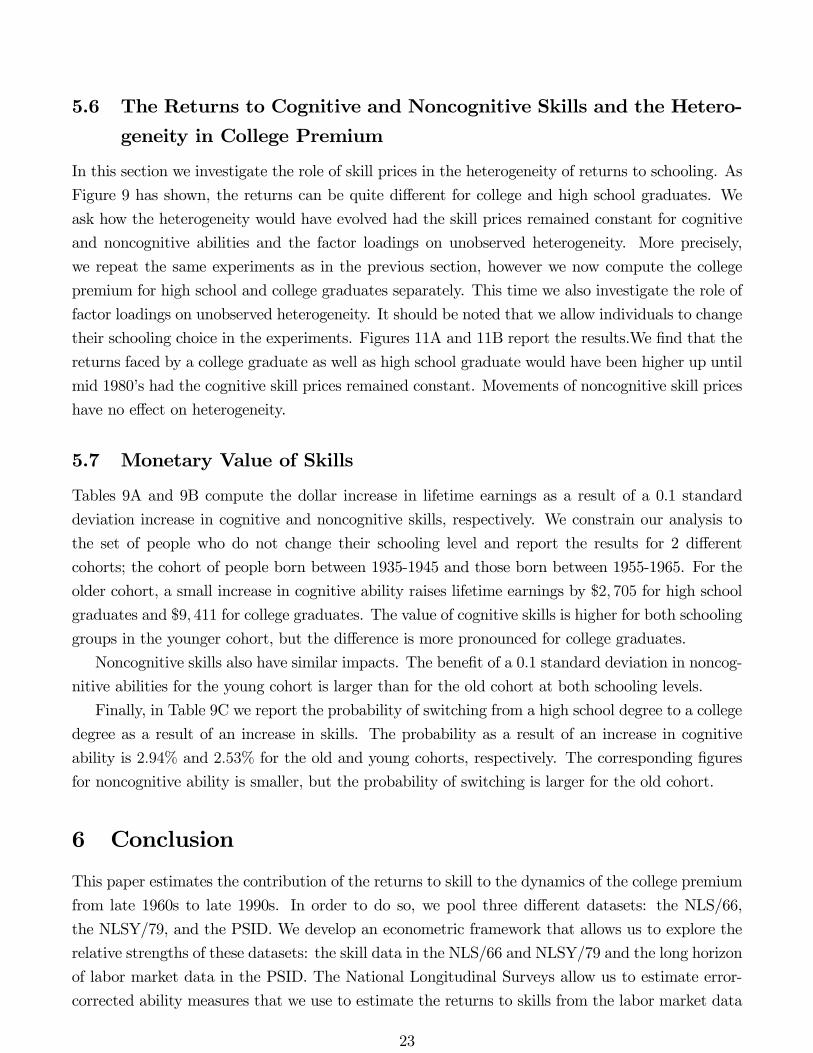
Figures 3A to 3D present some features of the Cognitive Test Scores regarding their relation with

parental education, number of siblings and schooling choice. Figures 3A to 3D show the same

analysis for the Noncognitive Test Scores.

In Figure 3A we have the partial correlation between each one of the cognitive test scores

and maternal education, controlling for urban and south residence, paternal education, number of

siblings, and cohort dummies. All but one of these tests exhibit positive partial correlation with

maternal education and this single negative correlation has a considerable part of its confidence

interval assuming positive values. It is worth to note the overlap of the confidence intervals of the

partial correlations for each of these tests with maternal education. If one draw a horizontal line

at 0.10 (as shown in the figure), this will cross all but one of the confidence intervals for the partial

correlation. A similar result is found in Figure 3B, now for the partial correlation between each

one of the cognitive test scores and paternal education, controlling for the same variables as before

and changing paternal for maternal education. Figures 3A and 3B together can be interpreted as

parental education having a positive relation with the individual performance in cognitive tests.

Figure 3C displays the partial correlations between each cognitive test score and the number of

siblings. The results point that, controlling for urban residence, south residence, parental education

and cohort dummies, individuals with higher cognitive test scores have, in general, fewer siblings. In

this case, there is a sub-interval common to all confidence intervals, so if one does the same exercise

of drawing a horizontal line, say at -0.04, this will cross all confidence intervals. The relation between

the cognitive test scores and the schooling choice appears in Figure 3D. These values correspond

to the coefficient of the specific cognitive test score in a probit regression, controlling for urban

and south residence, parental education, tuition costs and cohort dummies. This figure shows

that, in general, higher cognitive test scores are more likely to be associated to college graduates,

independent on the measure used. Even though the intersection of the confidence intervals for these

coefficients is less pronounced than in the past figures, we still observe some relation among the

different estimates.

Figures 4A to 4D are the analogous of 3A to 3D for the noncognitive test scores. In Figures 4A

and 4B we can see that as in the cognitive test scores case, the noncognitive tests also present a

consistent positive partial correlation with parental education, controlling for the same variables as

before. The similarities also hold for the intersections of the confidence intervals for the different

measures of noncognitive skills. As opposed to the case of cognitive tests, Figure 4C shows that,

10

if any, the relation between better performance in the noncognitive tests and number of siblings is

positive. Eight out of the ten measures studied exhibit a considerable intersection in the positive

axis of their confidence intervals for the partial correlation between noncognitive test scores and

number of siblings. Figure 4D reproduces the exercise done in Figure 3D, but now relating schooling

choice and noncognitive test scores. As in the former case, we can conclude that for all the analyzed

measures of cognitive skills, higher scores are more likely to be associated to college graduates than

to high school graduates.

3 The Econometric Framework

We now present a framework to analyze the pooled data described above. Specifically, our econo-

metric model addresses the issues that (i) skills are measured with error and in the PSID there

is only one (potentially very noisy) measure of cognitive skills; (ii) that individuals choose their

education levels and (iii) that their choice may be driven by skills as well as other observable and

unobservable characteristics of the individuals.

3.1 The Model for Labor Income

Let Ys,a,t denote the labor income of an individual who chooses schooling level s and is a years-old at

the calendar year t. Log earnings ys,a,t = lnYs,a,t are assumed to depend on observable characteristics

xs,a,t, cognitive and noncognitive skills (θc, θn), and unobservable components vs,a,t in the following

way:

ys,a,t = xs,a,tβs + αc,s,tθc + αn,s,tθn + vs,a,t (2)

The parameters βs depend on schooling choice, but we assume that they are constant over age

a and year t. The terms αc,s,t and αn,s,t are the returns to cognitive and noncognitive skills at

schooling level s and year t, respectively. The error terms vs,a,t are assumed to satisfy the condition

E (vs,a,t|xs,a,t, θc, θn) = 0, s = 0, 1; a = 1, ..., A; and t = 1, ..., T.We decompose the error terms in theearnings equations into a heterogeneity factor θh and an error term εs,a,t. The heterogeneity factor

may capture other dimensions of noncognitive skills that are orthogonal to "Locus of Control". We

denote by αh,s,t its factor loading. We assume that v0,a,t and v1,a,t can be written in factor-structure

form

vs,a,t = αh,s,tθh + εs,a,t s = 0, 1, t = 1, . . . , T. (3)

The idiosyncratic error term εs,a,t follows a structure with transition laws that are specific to school-

ing level s at period t: εs,a,t = πs,a,t + s,a,t, where πs,a,t follows an AR(1) process with persistence

ρs:

πs,a+1,t+1 = ρsπs,a,t + ηπs,a+1,t+1 (4)

11

and s,a,t follows an MA(1) process with coefficient φs:

s,a+1,t+1 = φsηs,a,t + ηs,a+1,t+1. (5)

3.2 The Schooling Choice Model

Agents make schooling choices based on expected present value utility maximization given infor-

mation set I. Let u (c) denote the agents utility when consumption is c. We assume that agents

cannot borrow or lend, so at each point in time consumption equals income:

cs,a,t = Ys,a,t = eys,a,t (6)

This assumption implies that consumption tracks income, which is at least partially consistent with

the data. For example, Carrol and Summers (1991) find that the growth rate of consumption is

larger for individuals that choose education levels also associated with higher income growth. The

same is true when they compare the life-cycle consumption profile of occupation groups that differ

in income growth. More recently, Fernandez-Villaverde and Krueger (2007) show that consumption

expenditure is hump shaped, especially when one does not drop the expenditure on durables. Fur-

thermore, consistent with the evidence from Carrol and Summers (1991), the hump shape profile is

more pronounced for individuals with higher levels of education. Fernandez-Villaverde and Krueger

(2010) offer an interpretation that the hump-shape profile of durable and nondurable consumption

expenditures could be explained by the lack of intertemporal markets for durable goods. This leads

households to build up their durable stocks little by little. Because durable and nondurable expen-

ditures interact in the budget constraint for a given time period, the way households finance the

expenditure on durables is by postponing some of the expenditure on nondurables. In this paper,

we do not model the consumption decision, primarily because both NLS/66 and NLSY/79 have no

information on consumption, while the PSID reports expenditures on food. In any case, we write

the index V as net present value of lifetime utility of graduating from college. Then:

V = E

"AXa=1

µ1

1 + ρ

¶a−1(u (c1,a,t)− u (c0,a,t))− C

¯¯I#, (7)

where C denotes the costs regarding a college education, which we decompose as

C = zγ + αc,Cθc + αn,Cθn + αh,Cθh + εC . (8)

Let θ = (θc, θn, θh) and αs,t = (αc,s,t, αn,s,t, αh,s,t) . In equation (8) z corresponds to observable

characteristics and the error term εC is independent of θ, x, z, εs,a,t, s = 0, 1, a = 1, ..., A, t =

1, . . . , T . We assume that x, z, θ, εC ∈ I, but that εs,a,t /∈ I, with E [εs,a,t| I] = 0 for all s, a, t. Let

12

x = {x0,a,t, x1,a,t}Aa=1 . Under these assumptions, it is easy to show that we can rewrite V as:

V = μ (x, z) + θα0V − εC (9)

where μ (x, z) =PA

a=1

³11+ρ

´a−1(x1,a,tβ1 − x0,a,tβ0) − zγ and α0V =

PAa=1

³11+ρ

´a−1 ¡α01,t − α00,t

¢−

α0C .

3.3 The Model for Cognitive and Noncognitive Test Scores

In addition to data on earnings and choices, we also have access to data on a set of cognitive

and noncognitive test scores. Let Mk,j denote the agent’s score on the kth test on skill j, where

j ∈ {c, n}. Assume that the Mk,j have finite means and can be expressed in terms of conditioning

variables XMk,j. Write

Mk,j = XMk,jβ

Mk,j + θjα

Mk,j + εMk,j and E

¡εMk,j¯θj,X

Mk,j

¢= 0. (10)

where the αMk,j are “factor loadings”, i.e. coefficients that map θj into Mk,j. Both the decision

to attend college and realized earnings likely depend on the cognitive and noncognitive skills that

agents have at the time their schooling choices are made. Following the psychometric literature, the

factors (θc, θn)might be interpreted as a latent cognitive and noncognitive abilities which potentially

affect all test scores. We assume that (θc, θn) is independent of XM =©XM

k,j

ªKj

k=1,j∈{c,n} and εMk,j,

withKj indicating the number of tests of skill j. The εMk,j are mutually independent and independent

of (θc, θn). Modeling test scores in this fashion allows them to be noisy measures of cognitive and

noncognitive abilities.10

4 Identification of Parameters

In this section we discuss identification of the model. We focus on parametric identification because

this is the estimation strategy that we pursue in the paper. We then discuss how the proof could be

extended to a semiparametric setting. More specifically, we assume that the factors are normally

distributed, so θ ∼ N (0,Σθ) . In what follows, we assume that the diagonal elements of Σθ are equal

to one. This is essentially a necessary normalization imposed on factor models because the scales

of the factors are never identified.

4.1 Identification of the Distribution of Skills

We start discussing identification of the test score equations, which are considerably easier. The

reason this is so is because we do not worry about selection issues with regard to the scores that are10The identification of the model can be secured under much weaker conditions by applying the analysis of Schen-

nach (2004).

13

observed in the data. As we show below, it is necessary to have at least three cognitive and three

noncognitive tests available in the dataset. We assume that the error terms εMk,j are independent

random variables that are normally distributed with mean zero and variance¡σMk,j

¢2. Under our

assumptions an OLS regression of the test score Mk,j against XMk,j identifies the parameters β

Mk,j.

Let Mk,j =Mk,j −XMk,jβ

Mk,j. We can compute the conditional covariances:

Cov³M1,c, M2,c

´= αM

1,cαM2,cV ar (θc) ,

Cov³M1,c, M3,c

´= αM

1,cαM3,cV ar (θc) ,

Cov³M2,c, M3,c

´= αM

2,cαM3,cV ar (θc) .

We imposed V ar (θc) = 1. We pick

αM1,c =

vuuutCov³M1,c, M2,c

´Cov

³M1,c, M3,c

´Cov

³M2,c, M3,c

´ .

We can recover αM2,c from Cov

³M1,c, M2,c

´and αM

3,c from Cov³M1,c, M3,c

´. The variances of the

error terms,¡σMk,c

¢2, are identified from V ar

³Mk,c

´. We can repeat the analysis for noncognitive

tests and identify the factor loadings.

The following moment identifies the covariance between cognitive and noncognitive skills:

Cov³M1,c, M1,n

´= αM

1,nαM1,nCov (θc, θn) . (11)

The identification of this covariance is interesting per se, but it is also important in the current

context because this is the only type of covariance that can be used to identify the factor loading

and variance of measurement error in the cognitive test that was given to the PSID respondents.

Obviously, identification requires Cov (θc, θn) 6= 0. Identification of these parameters can be war-

ranted even if such condition fails and we return to this issue when we discuss the identification of

the cognitive and noncognitive factor loadings in the schooling choice equation. If the cognitive and

noncognitive skill factors were the only factors in the model, then we would have already identified

the joint distribution of the factors exclusively from the information contained in the test score

equations. We will have more factors, so we will need to explore information from schooling choice

and log earnings to identify the distribution of the remaining factors. Although the approach de-

scribed here explores the parametric structure, it is possible to extend it to a nonparametric setting

by using the argument in Kotlarski (1967).

14

4.2 Identification of the Parameters in Earnings and Schooling Choice

Equations

The identification of the parameters in the log earnings and choice equations requires more work

because college log earnings are observed only for those individuals that chose to go to college. The

same problem is true for the high-school log earnings. Therefore, it is necessary to address the issue

of selection to obtain identification. To see how this arises in our model note that the mean college

earnings in the data are computed only using the subsample of those who chose to go college, which

is the sample equivalent of E (y1,a,t|x1,a,t, S = 1), but not E (y1,a,t|x1,a,t) . This implies that:

E (y1,a,t|x, z, S = 1) = x1,a,tβ1 +E¡θα01,t

¯x, z, S = 1

¢+E (ε1,a,t|x, z, S = 1) .

By assumption, ε1,a,t /∈ I with E (ε1,a,t| I) = 0. As a consequence, ε1,a,t does not affect schoolingchoices because it is not known at the time these choices are made. From (9) we know that

S = 1⇐⇒ εC − θα0V ≤ μ(x, z). Generally, this information is not very helpful because if we don’t

know the distribution of θ and εC , then we don’t obtain closed-form solutions for the conditional

moment E¡θα01,t

¯x, z, εC − θα0V ≤ μ(x, z)

¢. However, if the factors θ and the error term εC are

normally distributed it is possible to show that:

E¡θα01,t

¯x, z, εC − θα0V ≤ μ(x, z)

¢= −γ1,a,tκ (μ(x, z)) ,

where γ1,a,t =Cov(θα01,t,εC−θα0V )

V ar(εC−θα0V ), μ(x, z) = μ(x,z)

V ar(εC−θα0V ), κ (μ(x, z)) = φ(μ(x,z))

Φ(μ(x,z)), and the functions φ

and Φ are the density and distribution of standardized normal random variables. The mean college

log earnings equation satisfies:

E (y1,a,t|x, z, S = 1) = x1,a,tβ1 − γ1,a,tκ (μ(x, z)) .

If we knew the parameters that determine μ(x, z), then we could recover the parameters β1 and γ1,a,tfrom an OLS regression of y1,a,t against x1,a,t and κ (μ(x, z)) . Luckily, we can explore the information

from the schooling choice. Note that under normality assumptions Pr (S = 1|x, z) = Φ (μ(x, z))

and Pr (S = 0|x, z) = 1 − Φ (μ(x, z)) . By estimating this probit we can identify the parameters

that characterize μ(x, z). We use that information to recover β1 and γ1,a,t. This is the two-stage

estimation procedure developed in Heckman (1976). A similar analysis for the high-school log

earnings allows us to recover β0 and γ0,a,t.

15

4.2.1 Recovering the Loadings on Cognitive and Noncognitive Skills in Log EarningsEquations

Once identification of β0 and β1 have been secured, we can compute the following moments:

Cov³y1,a,t − x1,a,tβ1, M1,c

¯S = 1

´= αc,1,tα

M1,cV ar (θc|S = 1) + αn,1,tα

M1,cCov (θc, θn|S = 1)

Cov³y1,a,t − x1,a,tβ1, M1,n

¯S = 1

´= αc,1,tα

M1,nCov (θc, θn|S = 1) + αn,1,tα

M1,nV ar (θn|S = 1) .

There are two equations. The loadings αM1,c and αM

1,n have already been identified. Remember

that V ar (θc|S = 1) and V ar (θn|S = 1) are conditional variances of normally distributed randomvariables, so they can be easily estimated given our framework. If

αM1,cα

M1,n

¡V ar (θc|S = 1)V ar (θn|S = 1)− Cov (θc, θn|S = 1)2

¢6= 0,

then there are two linearly independent equations that generate a unique solution for the two un-

knowns, αc,1,t and αn,1,t. This argument identifies the factor loadings on cognitive and noncognitive

factors for all s, t pairs.

4.2.2 Recovering the Loadings on Cognitive and Noncognitive Skills in the SchoolingChoice Equation

A similar argument can be applied to identify the factor loadings on cognitive and noncognitive

skills on the schooling choice equation. As shown in Matzkin (1992), we can assume that we observe

net utility indexes V = V−μ(x,z)V ar(εC−θα0V )

and compute:

Cov³V , M1,c

´= αM

1,c

Ãαc,Vp

V ar (εC − θα0V )V ar (θc) +

αn,VpV ar (εC − θα0V )

Cov (θc, θn)

!

Cov³V , M1,n

´= αM

1,n

Ãαc,Vp

V ar (εC − θα0V )Cov (θc, θn) +

αn,VpV ar (εC − θα0V )

V ar (θn)

!

where αc,V and αn,V are the first two coordinates of the vector αV = (αc,V , αn,V , αh,V ). Given that

the loadings αM1,c and αM

1,n have already been identified, these covariances and the nonsingularity of

the covariance matrix of (θc, θn) allow us to identify the scaled factor loadingsαc,V

V ar(εC−θα0V )and

αn,V

V ar(εC−θα0V ).

At this point, we return to the issue regarding the identification of the factor loading and

variance of measurement error in the PSID cognitive test. If Cov (θc, θn) = 0, so that the moment

(11) cannot be used, then it is possible to identify the factor loading of the PSID test from the

covariance between schooling choice and the test score in PSID. Without loss of generality, let j = 4

16

denote the PSID cognitive test. Then, from the moment:

Cov³V , M4,c

´=

αM4,cαc,Vp

V ar (εC − θα0V )V ar (θc)

we can easily recover αM4,c.We can then use V ar

³M4,c

´to identify the variance of the measurement

error in the PSID cognitive test. Note that the existence of the schooling choice information,

together with a set of reliable estimates of skills from a different source, allows us to recover the

distribution of skills in the PSID free of measurement error even though we don’t have repeated

measures of skills in the PSID.

4.2.3 Recovering the Distribution of the Remaining Residual Components

In what follows, it will be convenient to define the residualized natural log earnings ys,a,t as:

ys,a,t = ys,a,t − xs,a,tβs − αc,s,tθc − αn,s,tθn = αh,s,tθh + πs,a,t + s,a,t

where πs,a,t and s,a,t follow the AR(1) and MA(1) processes defined in (4) and (5), respectively.

The identification of these components explore the time-series information within a schooling group.

Set αh,1,1 = 1 and define:

rs,a,l,k = Cov¡y1,a,l, y1,a+(k−l),k

¯S = 1

¢and note that the following equality holds:

r1,a+1,2,5 − αh,1,2r1,a,1,5r1,a+1,2,4 − αh,1,2r1,a,1,4

= ρ1 (12)

If we normalize αh,1,2 = 1, we could identify ρ1. However, such normalization may not be necessary

because of the following equality for every t = 5, 6, ..., T and k = 2, 3, ..., T also holds:

r1,a+1,k,t − αh,1,kr1,a,k,tr1,a+1,k,t−1 − αh,1,kr1,a,k,t−1

= ρ1 (13)

Focus on k = 2. We have the following polynomials in αh,1,2 :

b1,k,lα2h,1,2 − b2,k,lαh,1,2 + b3,k,l = 0

where

b1,k,l = (r1,a,1,kr1,a,1,l−1 − r1,a,1,lr1,a,1,k−1) ,

b2,k,l = (r1,a+1,2,kr1,a,1,l−1 + r1,a,1,kr1,a+1,2,l−1 − r1,a,1,k−1r1,a+1,2,l − r1,a+1,2,k−1r1,a,1,l) ,

b3,k,l = (r1,a+1,2,kr1,a+1,2,l−1 − r1,a+1,2,k−1r1,a+1,2,l) .

17

Clearly, if b1,k,l = 0, then there is only one solution for αh,1,2 =b3,k,lb2,k,l

. If b1,k,l 6= 0, then we have asecond-degree polynomial that may not have a real solution or may have at most two solutions that

are given by:

αh,1,2 =b2,k,l ±

qb22,k,l − 4b1,k,lb3,k,l2b1,k,l

If b22,k,l−4b1,k,lb3,k,l < 0, there are no real solutions. Note that this case happens if b22,k,l−4b1,k,lb3,k,l <0 for all possible combinations of k and l, an unlikely case. If b22,k,l − 4b1,k,lb3,k,l = 0, then there isone solution given by αh,1,2 =

b2,k,l2b1,k,l

. Finally, if b22,k,l − 4b1,k,lb3,k,l > 0, there are two solutions. We

pick the largest solution αh,1,2 =b2,k,l+

√b22,k,l−4b1,k,lb3,k,l2b1,k,l

. Once αh,1,2 is identified, we can identify ρ1

from (12). More importantly, we can use the relationship (13) to identify αh,1,k for k = 3, 4, ..., T.

Define σ2πt = V ar (πt) , σ2h,1 = V ar (θh|S = 1) . We can recover σ2h,1 from:

σ2h,1 =rs,a+1,1,4 − ρ1rs,a,1,3α1,4,h − ρ1α1,3,h

.

We identify the variance of the AR(1) component σ2πl , l = 1, 2, ..., T from:

rs,a,l,l+2 = α1,l,hαh,1,l+2σ2h,1 + ρ21σ

2πl.

We can use the fact that ρ1 and σ2πlare known, as well as the parametric formulation of the AR(1)

process, to identify the variance of shocks in the AR(1) component:

σ2πl+1 = ρ21σ2πl+ V ar

¡ηπs,a+1,t+1

¢.

We have to identify the variance of the MA(1) component as well as the persistence. From

V ar (ys,a,1) we identify V ar¡ηs,a,1

¢. Then, from rs,a,1,2, we identify φ1. This shows that all the

parameters for the labor income equation in the schooling group S = 1 are identified.

To guarantee identification of the parameters for schooling group S = 0, note that γ1,a,t =Cov(θα01,t,εC−θα0V )

V ar(εC−θα0V )is identified as well as each of the factor loadings in the vector α01,t. Normalizing

V ar (εC) = 1, we can then recover V ar (εC − θα0V ) =

µCov(θα01,t,εC−θα0V )

γ1,a,t

¶2. Given that information,

we can recover α0V without the scalepV ar (εC − θα0V ). We explore the covariance between labor

income in schooling S = 0 and the indexes from the schooling choice to identify αh,0,1. Once this

parameter is identified, we can repeat the argument made for S = 1 to identify the remaining

parameters for S = 0.

18

5 Empirical Results

5.1 Measurement Error in Ability Tests

One of the advantages of our approach is that we allow for the different tests that appraise abilities

to be measured with error. Note that there are two components in the residuals of the test score

equations (10). The first component is the cognitive or noncognitive factor pre-multiplied by its

factor loading. The second component is the measurement error from the tests. Under our assump-

tions, these two components are independent so we can assign the share of the residual variance

that is due to ability (i.e., due to θc or θn) and the one that is due to noise (i.e., due to εMk,j in

equation 10). Conditional on observed characteristics XMk,j, the total variance in test score k is:

V ar¡Mk,j|XM

k,j

¢=¡αMk,j

¢2V ar (θj) + V ar

¡εMk,j

¢The share of the variance that is due to true ability is V ar(θj)

V ar(Mk,j|XMk,j)

while the share that is due to

noise isV ar(εMk,j )

V ar(Mk,j|XMk,j)

. Figure 5 plots these quantities for each test used in our estimation. In terms

of cognitive skills, it is easy to see that the ASVAB components have the highest signal to noise

ratio. In fact, the Arithmetic Reasoning (ASVAB-AR) and Mathematical Knowledge (ASVAB-

MK) components have a signal ratio around 80 percent. The ASVAB measure that has the lowest

signal ratio is the Coding Speed (ASVAB-CS), around 40 percent, which is above the signal ratio

of the PSID sentence completion test (around 35 percent). The ACT, collected for the NLSY/79

and NLS/66 also exhibits high signal ratio (above 60 percent). The Occupation component in the

Knowledge of theWorld of Work, also collected for the NLSY/79 and NLS/66, presents a signal ratio

above 40 percent, well above that of the SAT (signal ratio of 10 percent) or the Lorge-Thorndike

test (8 percent). Our analysis shows a clear picture: the measures of ability from the NLSY/79

have the best signal to noise ratio, followed by the ones in the NLS/66, and lastly, by the PSID

measure.

None of the tests designed to measure noncognitive skills have signal ratios that are as high as

the components of the ASVAB. In fact, the components of the Rotter Locus of Control have signal

ratios at most around 30 percent (the PSID Rotter F component), and sometimes as low as 10

percent (the PSID Job Preference component).

5.2 The Estimates of the Schooling Choice Equation

These measures of skills are used to estimate the distributions of the cognitive and noncognitive

skill factors, which we then use to see how they affect schooling choices and labor income. Table 5

shows the estimates of the schooling cost equation (8). As commonly found in the literature (e.g.,

Cunha, Heckman, and Navarro 2005), the higher the education of the mother, the lower the psychic

costs of attending college. Similarly, higher stocks of cognitive and noncognitive skills also tend to

19

decrease the psychic costs of college. Interestingly, the unobserved heterogeneity component is such

that it increases the psychic costs of college. This finding means that individuals that have high

amounts of θh are more likely to choose s = 0.

The pattern of selection by skills changes in a non-monotonic way across cohorts. For example,

in Table 6A we see that in the first cohort (individuals born between 1920 and 1929) 40 percent of

the individuals in college were at the highest quartile of cognitive skills. That figure is 35 percent

for the third cohort (the individuals born between 1940 and 1949) and 38 percent for the last cohort

(individuals born between 1970 and 1978). These movements are reproduced for noncognitive skills

(Table 6B), but the variation is much smaller. The opposite movement is seen in terms of unobserved

heterogeneity (Table 6C): there is first an increase and then a decrease in the proportion of college

graduates that come from the top quartile of θh. All in all, the evidence from Tables 6A, 6B, and

6C show is that the individuals at the margin of going to college were not at the top quartile of the

joint distribution of (θc, θn, θh).

5.3 Estimates of the Log Earnings Equation

In Table 7 we show the point estimates and the standard errors of coefficients on the control variables

in the log income equations in high school and college, respectively. The potential experience profile

is more concave in college than in high school. We also find evidence that the income profiles are

becoming flatter for more recent cohorts. We are particularly interested in the year dummies

because they are the empirical counterpart to the μs,t in equation (1). In Figure 6 we plot the point

estimates of the coefficients on year dummies, as well as bars indicating one standard-deviation in

each direction. To help see their evolution over time, we regress the coefficients on a quartic in

periods, where a period is defined to be calendar year minus 1968. From this figure we can see

that the year dummies in the two different sectors have followed roughly a parallel pattern, except

during the late 1960s and early 1970s when they follow the opposite directions, increasing in the

college sector and declining in the high school sector.

In Table 8 we display the point estimates and standard errors of the returns to ability and

the factor loadings associated with the unobserved heterogeneity factor. Because the unobserved

heterogeneity is a combination of many different characteristics, we do not discuss the estimates of

the factor loadings, but we register that they exhibit trends in both schooling levels.

Figure 7A plots the estimated returns to cognitive ability in high school and college over the

period between 1968 and 2001. In the high school sector, one standard deviation in cognitive skills

is associated with an increase in income of 4.6 percent and there is little variation over the 33 year

window that our data covers. This contrasts starkly with the returns to cognitive skills. In late

1960s, one standard deviation in cognitive skills raised labor income by almost 9 percent. By 1980,

that return had already dropped to 1.5 percent. Ten years later, the return to cognitive skills had

jumped to 13.7 percent and it maintains around this plateau until the end of that decade. It is

20

very hard to miss the similarity of the dynamics of the college premium and that of the returns to

cognitive ability in the college sector.

Figure 7B plots the dynamics of the returns to noncognitive abilities in the high school and

college sector. We find that the returns are flat over the entire period covered by our data in

both college and high school. In any case, one standard deviation in noncognitive ability in the

high-school sector raises labor income by 7.7 percent. This is 68 percent higher than the impact

an equivalent change in cognitive skills. In the college sector, one standard deviation increase in

noncognitive skills causes income to increase by 9.3 percent.

5.4 The Evolution of College Premium and the Importance of Compo-

sitional Changes

In this section we quantify the importance of compositional changes in measuring the college pre-

mium. The literature studying the evolution of college premium has focussed on the observed wage

differentials between college and high school graduates. However, such differences are confounded

by the fact that college graduates are a selected sample of the population. Depending on the mar-

ket structure, one would expect individuals with higher expected returns to end up with college

degrees. This creates a wedge between the return of obtaining a college degree and the observed

wage differences among these groups. Moreover, as the importance of skills change over time, the

composition of college graduates may change, too. Therefore, the analysis would not only be biased

in the level of the returns to college but also in its evolution over time. The benefit of our approach

is the ability to correct for such compositional changes.

In order to evaluate how much selection matters for the assessment of college premium, we

simulate data from our model. The estimation of the model discussed in the previous sections

makes it possible to simulate earnings of an individual, yis,a,t, for both schooling levels. Using the

simulated data, we calculate the returns to schooling over time as rt = E£log yi1,a,t − log yi0,a,t | t

¤.

This represents college premium after collecting for selection.

Figure 8 plots rt and compares its evolution to the Mincerian returns reported before in Figure

1. We find differences along several dimensions. First, ignoring selection introduces, as expected,

an upward bias for the estimate of college premium: The Mincerian return is consistently larger

than the actual returns throughout the sample period. The difference gets smaller in the late 70’s,

but then widens up later on.

Second, the time-series pattern of the college premium also differs from the Mincerian counter-

part. Unlike the Mincerian returns, the corrected returns show an increase during 1970’s. Moreover,

while the Mincerian returns point to a sharply increasing profile during 1980’s, we find a less steeper

rise during that period. Both of the returns flatten out toward the end of the sample period.

Another interesting result of the estimation is the heterogeneity in the returns to college. Our

model allows the returns to schooling to be different across different people. This is possible because

21

of the observed heterogeneity in cognitive and noncognitive skills and the unobserved heterogene-

ity. Different prices of these components across education groups introduces heterogeneity in the

premium that one would obtain from obtaining a college degree. In particular, the sample of col-

lege graduates face different returns from college education than do the high school graduates. To

quantify how different the returns are, we compute expected returns for college and high school

graduates separately. More specifically, we compute r1,t = E£log yi1,a,t − log yi0,a,t | t, s = 1

¤and

r0,t = E£log yi1,a,t − log yi0,a,t | t, s = 0

¤. Figure 9 plots these returns.

The results show that the returns have been higher for college graduates for the entire sample

period. This happens because, on average, individuals with higher cognitive and noncognitive

abilities end up with a college degree and because the skill prices are higher for college graduates,

as shown in Figure 7A and 7B. The difference between the two schooling groups is smaller in the

early 70’s. This is consistent with the fact that the discrepancy between the Mincerian and corrected

returns in Figure 8 is smaller in the same period. We also find that the average return for college

graduates has diverged from that of the high school graduates, especially in the 1980’s.

5.5 The Returns to Cognitive and Noncognitive Skills and the Rise in

the College Premium

It has been suggested that the rise in the college premium can be due to the changes in the prices of

skills (Juhn, Murphy and Pierce, 1993). The model presented in this paper together with the data

we construct allows us to evaluate this hypothesis. To do so, we ask how much the college premium

would have changed if the skill prices had remained constant throughout the sample period. To

isolate the role of cognitive and noncognitive skills separately, we run 3 counterfactual experiments.

First, we constrain the price of cognitive skills for both schooling groups to remain constant at its

value in 1968 but leave everything else unaltered. Then, we repeat this for the price of noncognitive

skills. Finally, we ask how much of the change in college premium can be accounted for by changes

that are the same for both schooling groups. To answer this question, we set the coefficients on

time dummies to their values in 1968. In each of these counterfactuals, we simulate artificial data

from the model and compute average college premium as explained in the previous section.

Figure 10 plots the results. It is evident that the changes in the prices of cognitive skills have

had a significant effect on college premium. In particular, the college premium would have been

higher up until mid 1980’s and lower in the 1990’s if skill prices did not change at all. Changes in

noncognitive skill prices, on the other hand, cannot account for an important part of the college

premium. It is interesting that time dummies have a substantial effect on college premium. Our

analysis reveals that the college premium would have been mostly flat, if not decreasing, up until

1980’s if there was no change in the coefficients of time dummies. This implies that a large portion

of the changes in college premium since 1970’s are due to changes that are common to everyone in

the economy, regardless of their abilities.

22

5.6 The Returns to Cognitive and Noncognitive Skills and the Hetero-

geneity in College Premium

In this section we investigate the role of skill prices in the heterogeneity of returns to schooling. As

Figure 9 has shown, the returns can be quite different for college and high school graduates. We

ask how the heterogeneity would have evolved had the skill prices remained constant for cognitive

and noncognitive abilities and the factor loadings on unobserved heterogeneity. More precisely,

we repeat the same experiments as in the previous section, however we now compute the college

premium for high school and college graduates separately. This time we also investigate the role of

factor loadings on unobserved heterogeneity. It should be noted that we allow individuals to change

their schooling choice in the experiments. Figures 11A and 11B report the results.We find that the

returns faced by a college graduate as well as high school graduate would have been higher up until

mid 1980’s had the cognitive skill prices remained constant. Movements of noncognitive skill prices

have no effect on heterogeneity.

5.7 Monetary Value of Skills

Tables 9A and 9B compute the dollar increase in lifetime earnings as a result of a 0.1 standard

deviation increase in cognitive and noncognitive skills, respectively. We constrain our analysis to

the set of people who do not change their schooling level and report the results for 2 different

cohorts; the cohort of people born between 1935-1945 and those born between 1955-1965. For the

older cohort, a small increase in cognitive ability raises lifetime earnings by $2, 705 for high school

graduates and $9, 411 for college graduates. The value of cognitive skills is higher for both schooling

groups in the younger cohort, but the difference is more pronounced for college graduates.

Noncognitive skills also have similar impacts. The benefit of a 0.1 standard deviation in noncog-

nitive abilities for the young cohort is larger than for the old cohort at both schooling levels.

Finally, in Table 9C we report the probability of switching from a high school degree to a college

degree as a result of an increase in skills. The probability as a result of an increase in cognitive

ability is 2.94% and 2.53% for the old and young cohorts, respectively. The corresponding figures

for noncognitive ability is smaller, but the probability of switching is larger for the old cohort.

6 Conclusion

This paper estimates the contribution of the returns to skill to the dynamics of the college premium

from late 1960s to late 1990s. In order to do so, we pool three different datasets: the NLS/66,

the NLSY/79, and the PSID. We develop an econometric framework that allows us to explore the

relative strengths of these datasets: the skill data in the NLS/66 and NLSY/79 and the long horizon

of labor market data in the PSID. The National Longitudinal Surveys allow us to estimate error-

corrected ability measures that we use to estimate the returns to skills from the labor market data

23

over many different years and cohorts in the PSID, NLS/66 and NLSY/79.

We find that the dynamics of the returns to cognitive skills in the college sector are remarkably

similar to that of the college premium: the returns decrease during the 1970s, suddenly increase

in the 1980s, and continue to grow at a lower rate during the 1990s. We don’t find evidence of

trends in returns to cognitive skills in the high school sector or to noncognitive skills in high school

or college sectors. Composition changes also contribute to the dynamics of the college premium

and its role is particularly important in the 1990s. Nothwithstanding these findings, our results

indicate that most of the increase in the college premium is driven by the increase in μ1,τ −μ0,τ . Wealso estimate the factual college premium for actual college workers and the counterfactual college

premium for the high school workers. We find that they were about the same in the early 1970s

and they diverge in the early 1980s: the college premium goes up for college workers and remains

constant for the high school workers and only starts to go up for this group in the late 1980s. This

fact is substantially driven by the increase in the returns to cognitive skills.

24

7 References

Atkinson, John W. (1964) An Introduction to Motivation. Princeton, NJ.: Van Nostrand.

Autor, David H, Lawrence F. Katz, andMelissa S. Kearney. (2008) “Trends in U.S. Wage Inequality:

Re-Assessing the Revisionists,” Review of Economics and Statistics 90(2), 300-323.

Bishop, John H. (1991) "On-the-Job Training of New Hires." In Market Failure in Training, edited

by David Stern and Jozef M. M. Ritzen, New York, Springer Verlag, 61-96.

Blackburn, McKinley, and David Neumark. (1993) "Omitted-Ability Bias and the Increase in the

Return to Schooling." Journal of Labor Economics, July, 11:3, 521-44.

Borghans, Lex, Angela Lee Duckworth, James J. Heckman, and Bas ter Weel. (2008) "The eco-

nomics and psychology of personality traits." Journal of Human Resources, 43(4), 972-1059.

Bouchard, Thomas, and John Loehlin. (2001) "Genes, evolution, and personality." Behavior Ge-

netics, 31, 243-273.

Bowles, Samuel, and Herbert Gintis. (1976) Schooling in capitalist America: Educational reform

and contradictions of economic life. New York, NY: Basic Books.

Caliendo, Marco, Deborah Cobb-Clark, and Arne Uhlendorff. (2010) "Locus of Control and Job

Search Strategies." IZA Discussion Paper 4750.

Cameron, Stephen and James J. Heckman. (2001) "The Dynamics of Educational Attainment for

Black, Hispanic, and White Males." Journal of Political Economy, vol. 109(3), 455-459.

Card, David and Thomas Lemieux. (2001) "Can Falling Supply Explain The Rising Return To

College For Younger Men? A Cohort-Based Analysis." The Quarterly Journal of Economics, vol.

116(2), 705-746.

Carneiro, Pedro, Karsten T. Hansen, and James J. Heckman. (2003) "Estimating Distribution of

Counterfactuals with an Application to the Returns to Schooling and Measurement of the Effect of

Uncertainty on Schooling Choice." International Economic Review, Vol 44(2), 361-422.

Carneiro, Pedro, and Sokbae Lee. (2008) "Trends in Quality Adjusted Skill Premia in the US:

1960-2000." Working paper, UCL.

Carroll, Christopher, and Lawrence Summers. (1991) "Consumption Growth Parallels Income

Growth: SomeNew Evidence." In National saving and Economic Performance, edited by Douglas

Bernheim and John B. Shoven, Chicago University Press, 305—43.

Claessens, Amy, Greg Duncan, and Mimi Engel. (2009) "Kindergarten Skills and Fifth Grade

Achievement: Evidence from the ECLS-K." Economics of Education Review, 28(4): 415-427.

Chay, Kenneth Y., and David S. Lee. (2000) "Changes in relative wages in the 1980s Returns to

observed and unobserved skills and black-white wage differentials," Journal of Econometrics, 99(1):

1-38.

Cunha, Flavio, James J. Heckman, and Salvador Navarro. (2005) "Separating uncertainty from

heterogeneity in life cycle earnings." Oxford Economic Papers, Oxford University Press, vol. 57(2),

191-261.

25

Dunifon, Rachel, and Greg Duncan (1998) "Long-Run Effects of Motivation on Labor-Market Suc-

cess." Social Psychology Quarterly, 61(1): 33-48.

Edwards, Rick. (1976) "Individual Traits and Organizational Incentives: What makes a ’Good’

Worker?" Journal of Human Resources, 11(1), 51-68.

Fernandez-Villaverde, Jesus and Dirk Krueger. (2007) "Consumption over the Life Cycle: Some

Facts from Consumer Expenditure Survey Data." The Review of Economics and Statistics, 89(3):

552—565.

Fernandez-Villaverde, Jesus and Dirk Krueger. (2010) "Consumption and Saving over the Life

Cycle: How Important are Consumer Durables." Macroeconomic Dynamics, forthcoming.

Goldstein, Gerald, andMichel Hersen. (2000)Handbook of Psychological Assessment, Third Edition.

Oxford, UK: Elsevier.

Hansen, Karsten, James J. Heckman, and Kathleen Mullen. (2004) "The effect of schooling and

ability on achievement test scores." Journal of Econometrics, vol. 121(1-2), pages 39-98.

Heckman, James J. (1976) "The Common Structure of Statistical Models of Truncation, Sample

Selection and Limited Dependent Variables and a Simple Estimator for Such Models." The Annals

of Economic and Social Measurement, 5, 475-492.

Heckman, James J., and Edward Vytlacil. (2001) "Identifying the Role of Cognitive Ability in

Explaining the Level of and Change in the Return to Schooling."Review of Economics and Statistics,

Vol 83(1), 1-12.

Heckman, James, Jora Stixrud, and Sergio Urzua. (2006) "The Effects of Cognitive and Noncogni-

tive Abilities on Labor Market Outcomes and Social Behavior." Journal of Labor Economics, vol.

24(3), 411-482.

Juhn, Chinhui, Kevin Murphy, and Brooks Pierce. (1993) "Wage Inequality and the Rise in Returns

to Skill." Journal of Political Economy, 101(3), 410-42.

Katz, Lawrence and David Autor. (1999) "Changes in theWage Structure and Earnings Inequality."

In Handbook of Labor Economics, edited by Orley Ashenfelter and David Card, vol. 3A, North-

Holland, 1463-1555.

Katz, Lawrence and Kevin Murphy. (1992) "Changes in Relative Wages, 1963-1987: Supply and

Demand Factors." Quarterly Journal of Economics, 107, 35-78.

Klein, Roger, Richard Spady, and Andrew Weiss. (1991) "Factors Affecting the Output and Quit

Propensities of Production Workers." Review of Economic Studies, 58(2), 929-54.

Kotlarski, Ignacy. (1967) "On characterizing the gamma and normal distribution." Pacific Journal

of Mathematics, 20, 729-38.

Lorge, Irving and Robert Thorndike. (1966) Lorge-Thorndike Intelligence Tests. Chicago, IL:

Riverside Publishing Co.

Matzkin, Roza. (1992) "Nonparametric and distribution-free estimation of the binary threshold

crossing and the binary choice models." Econometrica, 60, 239-70.

McClelland, David, John Atkinson, Russell Clark, and Edgar Lowell. (1953) The achievement mo-

26

tive. New York, NY: Appleton-Century-Crofts.

Miller, Shawn. (2004) National Longitudinal Surveys: NLSY79 User’s Guide 1979-2002. Center for

Human Resource Research, The Ohio State University.

Mincer, Jacob. (1974) Schooling, Experience, and Earnings.New York, NY: Columbia University

Press.

Murnane, Richard J., John B. Willett, and Frank Levy. (1995) "The Growing Importance of

Cognitive Skills in Wage Determination." The Review of Economics and Statistics, vol. 77(2),

251-66.

Murray, Henry. (1938) Explorations in Personality. New York, NY: Oxford University Press.

Neal, Derek A., and William R. Johnson. (1996) "The Role of Premarket Factors in Black-White

Wage Differences." Journal of Political Economy, 104(5), 869-95.

Neisser, Ulric, Gwyneth Boodoo, Thomas J. Bouchard, A. Wade Boykin, Nathan Brody, Stephen J.

Ceci, Diane F. Halpern, John C. Loehlin, Robert Perloff, Robert J. Sternberg, and Susana Urbina.

(1996) "Intelligence: Knowns and Unknowns." American Psychologist 51(2):77—101.

Otis, Arthur S., and Roger T. Lennon. (1977)Otis-Lennon School Ability Test. New York: Harcourt

Brace Jovanovich.

Rotter, Julian B. (1966) "Generalized expectancies of internal versus external control of reinforce-

ments." Psychological Monographs, 80 (whole no. 609).

Rotter, Julian B. (1975) "Some problems and misconceptions related to the construct of internal

versus external control of reinforcement." Journal of Consulting and Clinical Psychology, 43, 56-67.

Schennach, Susanne. (2004) "Estimation of Nonlinear Models with Measurement Error." Econo-

metrica. 72, 33-75.

Sternberg, Robert. (1985) "Beyond IQ: A triarchic theory of human intelligence." New York, NY:

Cambridge University Press.

Taber, Christopher R. (2001) "The Rising College Premium in the Eighties: Return to College or

Return to Unobserved Ability." Review of Economic Studies, Vol 68, 665 - 691.

Traxler, Arthur. (1939) "A Study of the California Test of Mental Maturity: Advanced Battery."

The Journal of Educational Research, 32(5), 329-335.

Vane, Julia and Robert Motta. (1984) "Group Intelligence Tests." In Handbook of Psychological As-

sessment, edited by Gerald Goldstein and Michel Hersen (eds.), 100-116, Elmsford, NY: Pergamon

Press.

Veroff, Joseph, Lor McClelland and Kent Marquis. (1971) "Measuring intelligence and achievement

motivation in surveys." In Final Report to the U.S. Department of Health, Education, and Welfare,

Office of Economic Opportunity, Survey Research Center, Institute for Social Research, University

of Michigan, Ann Arbor Contract OEO-4180 .

27

0.35

0.40

0.45

0.50

0.55

0.60

0.65

Figure 1College Premium by Year

White Males for PSID, NLSY/79, and NLS/66

0.25

0.30

1968 1971 1974 1977 1980 1983 1986 1989 1992 1995 1998 2001

Specification 1 Specification 2 Quartic Approximation (Specification 1) Quartic Approximation (Specification 2)

This figure plots the estimated college premium by year according to two different specifications. In the first specification (gray diamonds),we regress log income year by year against a dummy for a college education and add potential experience, potential experience squared,dummies for south, urban residence at age 14, cohort dummies, and interactions of potential experience with cohort dummies. In the secondspecification (black squares), we regress log income in all years against a dummy for college education interacted with year dummies and addpotential experience, potential experience squared, dummies for south, urban residence at age 14, cohort dummies, and interactions of potential experience with cohort dummies. The solid curves are the quartic interpolation of the estimated college premium.

11.00

12.00

Figure 2ALog Labor Income Age Profile, High School

Comparison Across Different SurveysBars Indicate a One-Standard Deviation Above and Below

9.00

10.00

23 25 27 29 31 33 35 37 39 41 43 45 47 49 51 53 55

NLS/66 NLSY/79 PSID

Figure 2BLog Labor Income Age Profile, CollegeComparison Across Different Surveys

12.00

Bars Indicate a One-Standard Deviation Above and Below

11.00.00

10.00

9.00

23 25 27 29 31 33 35 37 39 41 43 45 47 49 51 53 55

NLS/66 NLSY/79 PSID

0 05

0.10

0.15

0.20

0.25

0.30

0.35

Figure 3APartial Correlation: Cognitive Test Scores and Maternal Education

White Males from PSID, NLS/66 and NLSY/79We control for urban and south residence, paternal education, number of siblings, and cohort

-0.05

0.00

0.05

Otis

-Len

non

Calif

orni

a Te

st o

f Men

tal M

atur

ity

Lorg

e-Th

ornd

ike

SAT

ACT

ASV

AB-

Arit

hmet

ic R

easo

ning

ASV

AB-

Wor

d K

now

ledg

e

ASV

AB-

Para

grap

h Co

mpo

sitio

n

ASV

AB-

Num

eric

al O

pera

tions

ASV

AB-

Codi

ng S

peed

ASV

AB-

Mat

h K

now

ledg

e

Wor

k K

now

ledg

e -O

ccup

atio

ns

Wor

k K

now

ledg

e -E

duca

tion

Wor

k K

now

ledg

e -E

arni

ngs

PSID

Sen

tenc

e Co

mpl

etio

n

Figure 3BPartial Correlation: Cognitive Test Scores and Paternal Education

White Males from PSID, NLS/66 and NLSY/79W ntr l f r rb n nd th r id n m t rn l d ti n n mb r f iblin nd h rt

0.30

0.35

We control for urban and south residence, maternal education, number of siblings, and cohort

0.20

0.25

0.05

0.10

0.15

-0.05

0.00

0.05

n y e T T g e n s d e s n s n

Otis

-Len

non

of M

enta

l Mat

urity

Lorg

e-Th

ornd

ike

SAT

ACT

ithm

etic

Reas

onin

g

B-W

ord

Kno

wle

dge

grap

h Co

mpo

sitio

n

mer

ical

Ope

ratio

ns

VA

B-Co

ding

Spe

ed

B-M

ath

Kno

wle

dge

edge

-O

ccup

atio

ns

wle

dge

-Edu

catio

n

owle

dge

-Ear

ning

s

nten

ce C

ompl

etio

n

Calif

orni

a Tes

t

ASV

AB-

Ari

ASV

AB

ASV

AB-

Para

g

ASV

AB-

Num

ASV

ASV

AB

Wor

k K

now

le

Wor

k K

now

Wor

k K

no

PSID

Sen

Figure 3CPartial Correlation: Cognitive Test Scores and Number of Siblings

White Males from PSID, NLS/66 and NLSY/79W ntr l f r rb n r id n th r id n m t rn l nd p t rn l d ti n nd h rt

0.03

0.05

We control for urban residence, south residence, maternal and paternal education, and cohort

0 03

0.00

-0.05

-0.03

-0.10

-0.08

n ty ke T T g ge n ns d ge ns n gs n

Otis

-Len

non

t of M

enta

l Mat

urit

Lorg

e-Th

ornd

ik

SAT

ACT

rithm

etic

Reas

onin

g

B-W

ord

Kno

wle

dg

agra

ph C

ompo

sitio

n

umer

ical O

pera

tion

VA

B-Co

ding

Spe

ed

B-M

ath

Kno

wled

g

ledge

-O

ccup

atio

n

owle

dge

-Edu

catio

n

now

ledg

e -E

arni

ng

ente

nce

Com

plet

ion

Calif

orni

a Tes

t

ASV

AB-

Ar

ASV

AB

ASV

AB-

Para

ASV

AB-

Nu

ASV

ASV

AB

Wor

k K

now

l

Wor

k K

no

Wor

k K

n

PSID

Se

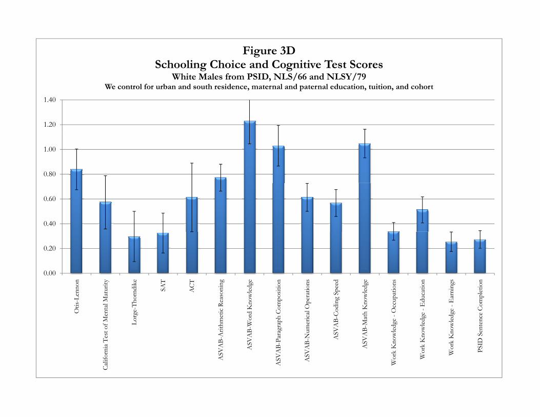
Figure 3DSchooling Choice and Cognitive Test Scores

White Males from PSID, NLS/66 and NLSY/79W ntr l f r rb n nd th r id n m t rn l nd p t rn l d ti n t iti n nd h rt

1.20

1.40

We control for urban and south residence, maternal and paternal education, tuition, and cohort

0.80

1.00

0.40

0.60

0.00

0.20

n y e T T g e n s d e s n s n

Otis

-Len

non

of M

enta

l Mat

urity

Lorg

e-Th

ornd

ike

SAT

ACT

ithm

etic

Reas

onin

g

B-W

ord

Kno

wle

dge

grap

h Co

mpo

sitio

n

mer

ical

Ope

ratio

ns

VA

B-Co

ding

Spe

ed

B-M

ath

Kno

wle

dge

edge

-O

ccup

atio

ns

wle

dge

-Edu

catio

n

owle

dge

-Ear

ning

s

nten

ce C

ompl

etio

n

Calif

orni

a Tes

t

ASV

AB-

Ar i

ASV

AB

ASV

AB-

Para

g

ASV

AB-

Num

ASV

ASV

AB

Wor

k K

now

le

Wor

k K

now

Wor

k K

no

PSID

Sen

Figure 4APartial Correlation: Noncognitive Test Scores and Maternal Education

White Males from PSID, NLS/66 and NLSY/79W l f b d h id l d i b f ibli d h

0.15

0.20

We control for urban and south residence, paternal education, number of siblings, and cohort

0.10

0.00

0.05

-0.05

-0.10

Rotte

r E

Rotte

r F

Rotte

r G

Rotte

r K

D R

otte

r E

D R

otte

r G

D P

lan L

ife

D R

otte

r F

ish T

hing

s

Pref

eren

ce

PSID

PSID

PSID

PSID

PSID

Fin

i

PSID

Job

P

0.10

0.15

0.20

0.25

0.30

0.35

Figure 4BPartial Correlation: Noncognitive Test Scores and Paternal Education

White Males from PSID, NLS/66 and NLSY/79We control for urban residence, south residence, maternal education, number of siblings, and cohort

-0.05

0.00

0.05

Rotte

r E

Rotte

r F

Rotte

r G

Rotte

r K

PSID

Rot

ter E

PSID

Rot

ter G

PSID

Plan

Life

PSID

Rot

ter F

PSID

Fin

ish T

hing

s

PSID

Job

Pref

eren

ce

Figure 4CPartial Correlation: Noncognitive Test Scores and Number of Siblings

White Males from PSID, NLS/66 and NLSY/79W ntr l f r rb n nd th r id n m t rn l nd p t rn l d ti n nd h rt

0.06

0.08

We control for urban and south residence, maternal and paternal education, and cohort

0.02

0.04

-0 02

0.00

-0.04

0.02

-0.06

Rotte

r E

Rotte

r F

Rotte

r G

Rotte

r K

D R

otte

r E

D R

otte

r G

D P

lan L

ife

D R

otte

r F

ish T

hing

s

Pref

eren

ce

PSID

PSID

PSID

PSID

PSID

Fin

i

PSID

Job

P

Figure 4DSchooling Choice and Noncognitive Test Scores

White Males from PSID, NLS/66 and NLSY/79W t l f b d th id t l d t l d ti t iti d h t

0.20We control for urban and south residence, maternal and paternal education, tuition, and cohort

0.10

0.15

0.05

0.00

-0.05

Rotte

r E

Rotte

r F

Rotte

r G

Rotte

r K

Rotte

r E

Rotte

r G

Plan

Life

Rotte

r F

h Th

ings

efer

ence

R R R R

PSID

R

PSID

R

PSID

P

PSID

R

PSID

Fin

ish

PSID

Job

Pre

Work Knowledge - OccupationsWork Knowledge - Education

Work Knowledge - EarningsPSID Sentence Completion

Rotter ERotter FRotter GRotter K

PSID Rotter EPSID Rotter GPSID Plan LifePSID Rotter F

PSID Finish ThingsPSID Job Preference

Figure 5Residual Variance in Test Scores: True Ability versus Noise

Cognitive and Noncognitive Skill Factors

0% 10% 20% 30% 40% 50% 60% 70% 80% 90% 100%

Otis-LennonLorge-Thorndike

California Test of Mental MaturitySATACT

ASVAB-ARASVAB-WKASVAB-PC

ASVAB-NOASVAB-CS

ASVAB-MK

True Ability Noise

-0.1

0.0

0.1

0.2

0.3

0.4

Figure 6Year Dummies in High School and College Sectors

-0.5

-0.4

-0.3

-0.2

1969 1972 1975 1978 1981 1984 1987 1990 1993 1996 1999

High School College Quartic Approximation (High School) Quartic Approximation (College)

0.10

0.14

0.18

Figure 7AReturns to Cognitive Ability

High School and College Sectors

‐0.02

0.02

0.06

1968 1972 1976 1980 1984 1988 1992 1996 2000

High School College Cubic Approximation (High School) Cubic Approximation (College)

0.10

0.14

0.18

Figure 7BReturns to Noncognitive AbilityHigh School and College Sectors

‐0.02

0.02

0.06

1968 1972 1976 1980 1984 1988 1992 1996 2000

High School College Cubic Approximation (High School) Cubic Approximation (College)

0.30

0.40

0.50

0.60

0.70

Figure 8Accounting for Compositional Changes in the College Premium

0.00

0.10

0.20

1968

1969

1970

1971

1972

1973

1974

1975

1976

1977

1978

1979

1980

1981

1982

1983

1984

1985

1986

1987

1988

1989

1990

1991

1992

1993

1994

1995

1996

1997

1998

1999

2000

2001

Mincer Corrected

Quartic Approximation (Mincer) Quartic Approximation (Corrected)

0.30

0.40

0.50

0.60

0.70

Figure 9The Dynamics of the College Premium

College Workers Versus High School Workers

0.00

0.10

0.20

1968

1969

1970

1971

1972

1973

1974

1975

1976

1977

1978

1979

1980

1981

1982

1983

1984

1985

1986

1987

1988

1989

1990

1991

1992

1993

1994

1995

1996

1997

1998

1999

2000

2001

Average College High School

Quartic Approximation (Average) Quartic Approximation (College) Quartic Approximation (High School)

0.30

0.40

0.50

0.60

0.70

Figure 10The College Premium, Returns to Skills, and Year Dummies

0.00

0.10

0.20

1968

1969

1970

1971

1972

1973

1974

1975

1976

1977

1978

1979

1980

1981

1982

1983

1984

1985

1986

1987

1988

1989

1990

1991

1992

1993

1994

1995

1996

1997

1998

1999

2000

2001

Returns Cognitive Time Dummies

Quartic Approximation (Returns) Quartic Approximation (Cognitive) Quartic Approximation (Dummies)

0.30

0.40

0.50

0.60

0.70

Figure 11AThe Dynamics of the College Premiumfor High School and College Workers

Factual versus Counterfactual Returns to Cognitive Skills

0.00

0.10

0.20

1968

1969

1970

1971

1972

1973

1974

1975

1976

1977

1978

1979

1980

1981

1982

1983

1984

1985

1986

1987

1988

1989

1990

1991

1992

1993

1995

1997

1999

2001

College High School

College (experiment) High School (experiment)

0.30

0.40

0.50

0.60

0.70

Figure 11BThe Dynamics of the College Premiumfor High School and College Workers

Factual versus Counterfactual Returns to Noncognitive Skills

0.00

0.10

0.20

1968

1969

1970

1971

1972

1973

1974

1975

1976

1977

1978

1979

1980

1981

1982

1983

1984

1985

1986

1987

1988

1989

1990

1991

1992

1993

1995

1997

1999

2001

College High School

College (experiment) High School (experiment)

age/year 1968 1969 1970 1971 1972 1973 1974 1975 1976 1977 1978 1979 1980 1981 1982 1983 1984 1985 1986 1987 1988 1989 1990 1991 1992 1993 1994 1995 1996 1997 1998 1999 2000 200123 73 77 136 145 155 3124 82 73 91 150 162 145 3325 141 94 89 93 167 164 15626 105 139 93 90 160 168 169 3527 102 146 91 96 170 160 16928 101 141 87 151 171 159 3529 100 87 91 146 155 154 3630 133 85 93 162 158 14131 94 81 87 139 148 14732 127 82 90 154 14733 86 119 83 138 14434 74 82 89 12635 111 76 8336 70 71 8137 106 7338 70 9839 684041424344454647484950515253545556

Lexis Diagram 1AData availability for Earnings (NLS/66)

Blue boxes mean available data for the corresponding age/year

age/year 1968 1969 1970 1971 1972 1973 1974 1975 1976 1977 1978 1979 1980 1981 1982 1983 1984 1985 1986 1987 1988 1989 1990 1991 1992 1993 1994 1995 1996 1997 1998 1999 2000 200123 113 120 132 160 134 167 131 12224 115 122 132 171 141 179 151 13525 121 126 137 168 147 179 159 13926 124 122 139 170 146 184 153 13827 124 125 142 182 150 183 156 13328 128 125 144 172 155 187 152 14029 127 126 145 178 153 181 153 14330 124 120 140 174 154 183 16131 128 129 138 168 150 184 14232 133 124 133 170 153 15833 132 121 132 170 180 12534 127 131 135 149 15235 124 125 164 169 13536 126 139 141 15537 130 166 158 12638 129 125 132 14239 119 167 15640 130 121 14041 110 14642 128 11443 11044 117454647484950515253545556

Lexis Diagram 1BData availability for Earnings (NLSY/79)

Blue boxes mean available data for the corresponding age/year

age/year 1968 1969 1970 1971 1972 1973 1974 1975 1976 1977 1978 1979 1980 1981 1982 1983 1984 1985 1986 1987 1988 1989 1990 1991 1992 1993 1994 1995 1996 1997 1998 1999 2000 200123 17 23 46 35 30 36 44 37 44 38 39 45 37 26 31 37 32 29 18 21 19 21 24 16 18 21 18 15 18 18 16 1624 21 33 32 62 52 44 48 56 43 58 40 48 50 44 29 38 41 42 38 27 29 26 24 29 21 29 22 24 24 23 22 2625 22 27 35 36 73 57 57 46 66 54 67 46 57 56 48 31 48 43 45 43 33 39 31 38 35 24 41 25 30 24 28 3626 28 24 33 38 45 79 63 59 47 71 56 70 51 64 62 59 34 55 44 53 48 40 47 35 38 38 26 44 33 29 41 3827 26 29 30 35 39 50 81 65 56 46 70 57 73 52 70 66 60 41 59 49 53 52 41 53 36 40 42 29 44 27 31 3828 19 29 34 31 35 42 54 89 65 63 48 69 59 76 53 76 65 63 40 61 54 56 57 42 55 39 41 44 32 42 31 4429 15 21 33 33 35 38 39 49 88 67 61 46 71 60 70 55 78 71 70 40 62 55 56 59 43 56 38 41 47 28 30 3430 20 17 24 34 32 37 41 41 49 86 67 64 48 70 59 74 52 81 74 68 42 64 55 53 59 47 52 36 43 40 40 3531 17 23 19 24 34 35 36 44 44 50 81 64 59 51 67 52 77 58 79 68 73 43 70 52 62 60 50 52 35 34 30 3732 17 22 23 19 25 34 36 36 44 45 49 81 65 54 49 64 49 75 59 76 71 73 49 70 55 58 60 47 53 24 41 4833 13 19 22 24 19 26 35 34 37 47 43 48 79 65 54 51 66 50 76 59 75 68 77 49 73 57 59 61 47 47 32 3334 19 13 20 22 24 19 25 32 36 38 46 43 49 75 69 57 53 61 50 76 59 73 69 72 50 67 57 58 56 40 28 4135 17 20 13 21 22 24 18 27 32 33 39 43 43 49 78 66 54 52 61 50 76 62 69 66 73 54 67 60 60 49 48 3436 18 16 20 13 21 22 24 16 28 35 35 39 43 41 44 75 67 50 54 63 51 78 64 71 68 73 55 70 60 50 37 2637 25 19 16 20 13 24 21 23 16 26 37 36 40 43 41 47 70 65 51 55 63 49 84 65 66 68 67 56 69 52 49 4838 28 26 20 17 21 14 24 20 21 16 26 37 34 40 42 38 46 72 64 53 54 60 51 79 67 68 62 69 56 58 48 3439 26 27 26 19 17 22 14 23 20 24 16 26 34 34 38 43 38 44 67 65 53 53 62 51 76 61 70 65 72 42 51 4440 29 26 26 26 20 17 22 14 22 20 20 16 24 32 34 34 41 37 44 69 62 49 54 58 50 72 59 68 63 54 59 4841 27 31 27 26 27 20 18 23 15 22 20 20 16 24 31 35 36 41 35 43 70 61 55 50 57 53 72 59 65 42 44 5242 21 25 30 28 26 27 21 18 23 15 23 21 20 14 24 29 38 39 41 38 42 63 65 55 45 54 51 71 59 59 56 5843 21 21 26 31 28 26 27 21 17 23 15 24 21 19 17 23 29 35 39 42 37 41 63 65 58 47 55 50 72 46 43 4444 17 22 22 26 30 28 26 23 21 18 24 15 23 21 16 19 22 30 31 38 42 35 44 62 63 53 51 51 53 53 54 5445 15 18 22 22 26 30 28 26 23 21 17 23 14 23 23 17 19 19 30 31 36 39 37 44 63 67 52 51 48 43 45 4246 22 16 18 23 22 26 31 27 25 21 22 16 23 14 22 22 17 18 22 30 31 34 37 39 44 65 63 50 47 44 48 5147 20 21 16 19 23 24 26 29 28 26 20 21 19 22 12 21 20 15 18 25 30 30 32 34 35 38 62 57 48 43 44 4348 15 19 21 16 19 24 23 23 27 27 25 22 22 19 21 11 21 19 16 17 25 31 30 31 34 34 41 63 57 39 41 5349 14 16 18 21 16 19 24 23 23 27 26 25 22 24 17 21 9 20 18 15 17 24 30 32 30 33 39 38 69 53 39 4550 14 14 16 19 20 15 19 23 22 23 26 26 25 22 24 16 21 8 20 20 14 17 27 30 33 28 27 34 36 56 43 4251 15 15 14 16 18 20 15 20 20 22 21 26 26 25 21 24 15 21 9 20 18 14 18 25 31 33 31 28 35 33 54 3652 9 16 15 14 17 19 20 15 18 19 21 22 26 26 24 20 22 14 19 9 20 18 13 18 24 31 28 25 27 31 52 3753 8 9 17 15 14 17 19 20 15 18 20 21 21 26 26 22 19 22 14 18 9 20 18 14 18 24 27 30 29 21 25 5254 11 8 10 17 14 14 17 20 19 14 18 20 19 21 26 24 21 18 20 14 20 9 20 18 13 16 21 26 31 23 33 5155 10 11 9 10 17 15 14 15 17 18 15 18 19 17 21 21 23 19 18 18 14 19 9 19 16 13 18 19 25 24 23 2356 11 9 11 9 10 17 15 14 13 16 18 15 19 18 17 21 22 21 21 17 19 13 20 7 18 17 11 17 20 21 24 31

Lexis Diagram 1CData availability for Earnings (PSID)

Blue boxes mean available data for the corresponding age/year

age/year 1968 1969 1970 1971 1972 1973 1974 1975 1976 1977 1978 1979 1980 1981 1982 1983 1984 1985 1986 1987 1988 1989 1990 1991 1992 1993 1994 1995 1996 1997 1998 1999 2000 200123 90 100 182 180 30 191 44 68 44 38 39 45 150 146 163 197 166 196 149 143 19 21 24 16 18 21 18 15 18 18 16 1624 103 106 123 212 52 206 48 201 76 58 40 48 50 159 151 170 212 183 217 178 164 26 24 29 21 29 22 24 24 23 22 2625 163 121 124 129 73 224 57 210 222 54 67 46 57 56 169 157 185 211 192 222 192 178 31 38 35 24 41 25 30 24 28 3626 133 163 126 128 45 239 63 227 216 71 91 70 51 64 62 183 156 194 214 199 232 193 185 35 38 38 26 44 33 29 41 3827 26 131 176 126 39 146 81 235 216 46 239 57 73 52 70 66 184 166 201 231 203 235 197 186 36 40 42 29 44 27 31 3828 19 29 135 172 35 129 54 240 236 63 207 69 94 76 53 76 65 191 165 205 226 211 244 194 195 39 41 44 32 42 31 4429 15 21 33 133 35 125 39 140 234 67 216 46 225 96 70 55 78 71 197 166 207 233 209 240 196 199 38 41 47 28 30 3430 20 17 24 34 32 170 41 126 142 86 229 64 206 211 59 74 52 81 74 192 162 204 229 207 242 208 52 36 43 40 40 3531 17 23 19 24 34 129 36 125 131 50 220 64 207 198 67 52 77 58 79 68 201 172 208 220 212 244 50 194 35 34 30 3732 17 22 23 19 25 34 36 163 126 45 139 81 219 201 49 64 49 75 59 76 71 206 173 203 225 211 60 205 53 24 41 4833 13 19 22 24 19 26 35 120 156 47 126 48 217 209 54 51 66 50 76 59 75 68 209 170 205 227 59 241 47 172 32 3334 19 13 20 22 24 19 25 32 110 38 128 43 138 201 69 57 53 61 50 76 59 73 69 199 181 202 57 207 56 192 28 4135 17 20 13 21 22 24 18 27 32 33 150 43 119 132 78 66 54 52 61 50 76 62 69 66 197 179 67 224 60 218 183 3436 18 16 20 13 21 22 24 16 28 35 105 39 114 122 44 75 67 50 54 63 51 78 64 71 68 199 55 209 60 191 192 2637 25 19 16 20 13 24 21 23 16 26 37 36 146 116 41 47 70 65 51 55 63 49 84 65 66 68 67 186 69 218 207 17438 28 26 20 17 21 14 24 20 21 16 26 37 104 138 42 38 46 72 64 53 54 60 51 79 67 68 62 198 56 183 180 17639 26 27 26 19 17 22 14 23 20 24 16 26 34 102 38 43 38 44 67 65 53 53 62 51 76 61 70 65 72 161 218 20040 29 26 26 26 20 17 22 14 22 20 20 16 24 32 34 34 41 37 44 69 62 49 54 58 50 72 59 68 63 184 180 18841 27 31 27 26 27 20 18 23 15 22 20 20 16 24 31 35 36 41 35 43 70 61 55 50 57 53 72 59 65 42 154 19842 21 25 30 28 26 27 21 18 23 15 23 21 20 14 24 29 38 39 41 38 42 63 65 55 45 54 51 71 59 59 184 17243 21 21 26 31 28 26 27 21 17 23 15 24 21 19 17 23 29 35 39 42 37 41 63 65 58 47 55 50 72 46 43 15444 17 22 22 26 30 28 26 23 21 18 24 15 23 21 16 19 22 30 31 38 42 35 44 62 63 53 51 51 53 53 54 17145 15 18 22 22 26 30 28 26 23 21 17 23 14 23 23 17 19 19 30 31 36 39 37 44 63 67 52 51 48 43 45 4246 22 16 18 23 22 26 31 27 25 21 22 16 23 14 22 22 17 18 22 30 31 34 37 39 44 65 63 50 47 44 48 5147 20 21 16 19 23 24 26 29 28 26 20 21 19 22 12 21 20 15 18 25 30 30 32 34 35 38 62 57 48 43 44 4348 15 19 21 16 19 24 23 23 27 27 25 22 22 19 21 11 21 19 16 17 25 31 30 31 34 34 41 63 57 39 41 5349 14 16 18 21 16 19 24 23 23 27 26 25 22 24 17 21 9 20 18 15 17 24 30 32 30 33 39 38 69 53 39 4550 14 14 16 19 20 15 19 23 22 23 26 26 25 22 24 16 21 8 20 20 14 17 27 30 33 28 27 34 36 56 43 4251 15 15 14 16 18 20 15 20 20 22 21 26 26 25 21 24 15 21 9 20 18 14 18 25 31 33 31 28 35 33 54 3652 9 16 15 14 17 19 20 15 18 19 21 22 26 26 24 20 22 14 19 9 20 18 13 18 24 31 28 25 27 31 52 3753 8 9 17 15 14 17 19 20 15 18 20 21 21 26 26 22 19 22 14 18 9 20 18 14 18 24 27 30 29 21 25 5254 11 8 10 17 14 14 17 20 19 14 18 20 19 21 26 24 21 18 20 14 20 9 20 18 13 16 21 26 31 23 33 5155 10 11 9 10 17 15 14 15 17 18 15 18 19 17 21 21 23 19 18 18 14 19 9 19 16 13 18 19 25 24 23 2356 11 9 11 9 10 17 15 14 13 16 18 15 19 18 17 21 22 21 21 17 19 13 20 7 18 17 11 17 20 21 24 31

Lexis Diagram 1DData availability for Earnings (Pooled Data)

Blue boxes mean available data for the corresponding age/year

Estimate Std. Error t-statisticCohort 01 (born before 1929) 0.374 0.028 13.57Cohort 02 (born between 1930 and 1939) 0.405 0.030 13.51Cohort 03 (born between 1940 and 1949) 0.508 0.016 32.1Cohort 04 (born between 1950 and 1959) 0.400 0.013 31.31Cohort 05 (born between 1960 and 1969) 0.396 0.016 24.98Cohort 06 (born between 1970 and 1978) 0.445 0.027 16.68Dummy for NLS/66 -0.039 0.018 -2.15Dummy for NLSY/79 -0.011 0.018 -0.63

Observations 6396R2 0.423F-test (Dummy for NLS/66 = 0 and Dummy for NLSY/79 = 0) 2.37P-Value of F-test 0.094

Table 1Fraction of Individuals with a College Degree

by Cohort and Survey*

*Note: To construct this table, we regress schooling attainment (s = 0 for high school graduates and s = 1 for college graduates) against cohort dummies and survey membership dummies.

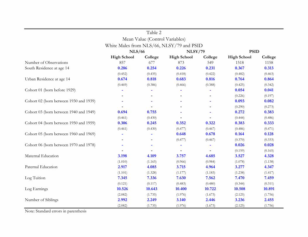
High School College High School College High School CollegeNumber of Observations 857 677 873 549 1518 1158South Residence at age 14 0.286 0.254 0.226 0.231 0.367 0.313

(0.452) (0.435) (0.418) (0.422) (0.482) (0.463)Urban Residence at age 14 0.674 0.818 0.683 0.816 0.764 0.864

(0.469) (0.386) (0.466) (0.388) (0.425) (0.342)Cohort 01 (born before 1929) - - - - 0.054 0.041

- - - - (0.226) (0.197)Cohort 02 (born between 1930 and 1939) - - - - 0.093 0.082

- - - - (0.290) (0.273)Cohort 03 (born between 1940 and 1949) 0.694 0.755 - - 0.272 0.383

(0.461) (0.430) - - (0.444) (0.486)Cohort 04 (born between 1950 and 1959) 0.306 0.245 0.352 0.322 0.383 0.333

(0.461) (0.430) (0.477) (0.467) (0.486) (0.471)Cohort 05 (born between 1960 and 1969) - - 0.648 0.678 0.164 0.128

- - (0.477) (0.467) (0.370) (0.333)Cohort 06 (born between 1970 and 1978) - - - - 0.026 0.028

- - - - (0.159) (0.165)Maternal Education 3.198 4.109 3.757 4.685 3.527 4.328

(1.010) (1.165) (0.966) (0.984) (1.078) (1.138)Paternal Education 2.917 4.085 3.715 4.964 3.277 4.347

(1.101) (1.328) (1.177) (1.183) (1.238) (1.417)Log Tuition 7.345 7.336 7.630 7.562 7.470 7.459

(0.121) (0.117) (0.483) (0.480) (0.344) (0.311)Log Earnings 10.526 10.643 10.400 10.722 10.508 10.891

(2.082) (1.735) (1.976) (1.673) (2.125) (1.756)Number of Siblings 2.992 2.249 3.140 2.446 3.236 2.455

(2.082) (1.735) (1.976) (1.673) (2.125) (1.756)Note: Standard errors in parenthesis

Mean Value (Control Variables)White Males from NLS/66, NLSY/79 and PSID

NLS/66 NLSY/79 PSID

Table 2

Q1 Q2 Q3 Q4 Q1 Q2 Q3 Q4

Otis-Lennon Test1 38.41% 34.77% 20.53% 6.29% 11.55% 10.76% 31.47% 46.22%California Mental Maturity Test2 37.70% 28.96% 19.67% 13.66% 10.08% 15.97% 32.77% 41.18%Lorge-Thorndike Test3 32.41% 34.26% 22.22% 11.11% 14.29% 12.99% 28.57% 44.16%Scholastic Aptitude Test (SAT)4 55.56% 17.28% 16.05% 11.11% 18.42% 27.11% 26.58% 27.89%American College Test (ACT)4 53.85% 28.21% 17.95% 0.00% 21.13% 24.74% 25.26% 28.87%ASVAB - Arithmetic Reasoning5 42.12% 27.11% 24.66% 6.11% 8.24% 17.42% 29.03% 45.32%ASVAB - Word Knowledge5 41.27% 29.18% 22.71% 6.84% 7.49% 15.36% 41.39% 35.77%ASVAB - Paragraph Composition5 41.15% 27.23% 27.59% 4.03% 6.18% 20.79% 57.68% 15.36%ASVAB - Numerical Operation5 36.26% 30.40% 20.39% 12.94% 8.05% 25.66% 26.78% 39.51%ASVAB - Coding Speed5 36.14% 28.08% 21.86% 13.92% 13.11% 21.54% 24.53% 40.82%ASVAB - Math Knowledge5 39.80% 38.10% 19.41% 2.69% 3.18% 13.11% 35.77% 47.94%Work knowledge, occupations knowledge6 34.90% 33.45% 21.86% 9.80% 13.96% 36.49% 30.12% 19.43%Work knowledge, education required for occupation6 34.99% 31.44% 20.21% 13.36% 13.82% 30.76% 22.73% 32.69%Work knowledge, earnings comparison6 51.06% 33.33% 0.00% 15.61% 32.59% 32.59% 0.00% 34.81%PSID Sentence Completion7 35.79% 26.55% 33.93% 3.73% 16.92% 20.12% 51.48% 11.48%

6 The Knowledge of World of Work test consists of three components. The first requires a respondent to identify, in a multiple-choice format, the duties of ten occupations. Thesecond component involves identification of the typical educational attainment of men in each of these same ten occupations. The third component is based on a respondent'sjudgment, for each of eight pairs of occupations, as to which one yields the higher average annual earnings. 7 PSID sentence completion test is an adaptation of the verbal component of the Lorge-Thorndike Intelligence Test.

1 The Otis-Lennon test Intends to provide a measure of IQ and is organized in five areas: verbal comprehension, verbal reasoning, pictorial reasoning, figural reasoning, andquantitative reasoning. 2 The California Test of Mental Maturity is designed to measure memory, spatial relationships, reasoning, and vocabulary. 3 The Lorge-Thorndike Intelligence Test measures abstract intelligence and contains both verbal and nonverbal items. 4 The Scholastic Aptitude Test (SAT) and the American College Test (ACT) are standardized tests used in college admissions in the United States. The SAT consists of threemajor sections: Critical Reading, Mathematics, and Writing. The American College Test (ACT) covers four skill areas: English, Mathematics, Reading, and Science.5 The ASVAB is a multiple choice test used to determine qualification for enlistment in the United States armed forces. The Arithmetic Reasoning Test measures an individual'sability to solve arithmetic word problems. The Word Knowledge component intends to measure the individual's ability to provide the correct meaning to a word that is presented in a context. The Paragraph Comprehension evaluates the capacity to understand written passages. The Numerical Operation test consists of a series of arithmetic computationsthat must be carried out correctly within a time limit. The Coding Speed component measures the capacity to assign code numbers to words. The Math Knowledge test measuresthe knowledge of high-school math principles.

White Males from NLS/66, NLSY/79 and PSIDHigh School College

Table 3Proportion of People in Each Quartile (Cognitive Skill Tests)

1 2 3 4 5 6 1 2 3 4 5 6

Rotter E1 13.63% 10.96% 27.64% 47.77% - - 10.48% 8.94% 28.79% 51.79% - -Rotter F2 24.46% 25.48% 20.08% 29.99% - - 15.60% 14.75% 30.26% 39.39% - -Rotter G3 9.13% 6.83% 38.29% 45.76% - - 5.83% 5.66% 39.42% 49.10% - -Rotter K4 22.19% 18.65% 33.61% 25.55% - - 18.27% 19.31% 39.13% 23.29% - -Rotter E PSID1 18.10% - - 81.90% - - 15.31% - - 84.69% - -Rotter G PSID3 29.88% 0.18% 0.62% 0.80% 68.51% - 17.64% - 0.95% 1.55% 79.86% -PSID Planning5 47.55% 0.45% 1.78% 1.16% 49.06% - 31.94% 1.19% 2.98% 2.74% 61.14% -Rotter F PSID2 0.09% 30.20% 0.09% 2.96% 0.99% 65.68% - 19.67% 0.59% 2.25% 1.54% 75.95%PSID Carrying-out Plans6 17.31% 0.09% 0.89% 1.07% 80.64% - 13.73% 0.12% 0.71% 0.83% 84.62% -PSID Affiliation vs Achievement7 35.57% - - 64.43% - - 19.15% - - 80.85% - -

6 "When you make plans ahead, do you usually get to carry out things the way you expected, or do things usually come up to make you change your plans?" There are five possibleanswers and higher values indicate individuals who report to be more likely to carry out plans to the end.7 "What kind of job would you want the most, a job where you had to think for yourself, or a job where the people you work with are a nice group?". There are two possible answers andthe highest value reflects individuals who are more likely to prefer a job that he can think for himself (i.e., lower need for affiliation).

Notes: 1 "What Happens to me is my own doing". There are four possible answers in the NLS/66 and NLSY/79 surveys and two possible answers in the PSID survey. Higher valuesindicate stronger internal locus of control.2 "I can make plans work". There are four possible answers in the NLS/66 and NLSY/79 surveys and five possible answers in the PSID survey. Higher values indicate stronger internallocus of control.3 "What I want has nothing do to with luck". There are four possible answers in the NLS/66 and NLSY/79 surveys and two possible answers in the PSID survey. Higher values indicatestronger internal locus of control.4 "It is impossible to believe that luck plays role". There are four possible answers in the NLS/66 and NLSY/79 surveys and is not available in the PSID survey. Higher values indicatestronger internal locus of control.5 "Are you the kind of person that plans his life ahead all the time, or do you live more from day to day?" There are five possible answers and higher values indicate individuals who reportare more likely to plan.

Table 4Proportion of People in Each Alternative (Noncognitive Skill Tests)

White Males from NLS/66, NLSY/79 and PSIDHigh School College

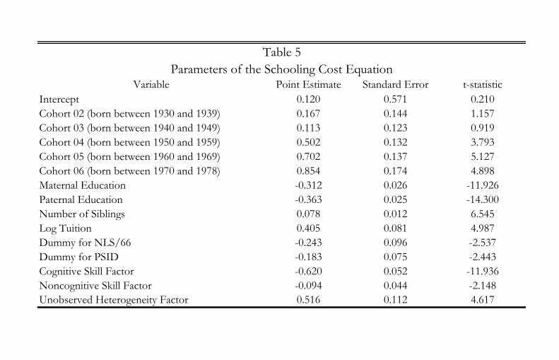
Variable Point Estimate Standard Error t-statisticIntercept 0.120 0.571 0.210Cohort 02 (born between 1930 and 1939) 0.167 0.144 1.157Cohort 03 (born between 1940 and 1949) 0.113 0.123 0.919Cohort 04 (born between 1950 and 1959) 0.502 0.132 3.793Cohort 05 (born between 1960 and 1969) 0.702 0.137 5.127Cohort 06 (born between 1970 and 1978) 0.854 0.174 4.898Maternal Education -0.312 0.026 -11.926Paternal Education -0.363 0.025 -14.300Number of Siblings 0.078 0.012 6.545Log Tuition 0.405 0.081 4.987Dummy for NLS/66 -0.243 0.096 -2.537Dummy for PSID -0.183 0.075 -2.443Cognitive Skill Factor -0.620 0.052 -11.936Noncognitive Skill Factor -0.094 0.044 -2.148Unobserved Heterogeneity Factor 0.516 0.112 4.617

Parameters of the Schooling Cost EquationTable 5

Q1 Q2 Q3 Q4 Q1 Q2 Q3 Q4Cohort 01 (born before 1929) 33.05% 27.52% 23.10% 16.33% 12.38% 20.49% 27.72% 39.41%Cohort 02 (born between 1930 and 1939) 33.47% 27.71% 22.82% 16.00% 12.90% 20.98% 28.21% 37.92%Cohort 03 (born between 1940 and 1949) 35.41% 27.97% 22.23% 14.38% 14.12% 21.69% 27.98% 36.21%Cohort 04 (born between 1950 and 1959) 33.26% 27.75% 23.08% 15.91% 12.39% 20.68% 28.03% 38.91%Cohort 05 (born between 1960 and 1969) 34.00% 27.97% 22.45% 15.57% 12.22% 20.99% 27.99% 38.80%Cohort 06 (born between 1970 and 1978) 33.98% 28.67% 22.65% 14.70% 12.79% 20.30% 28.68% 38.23%

Table 6AProportion of People in Each Quartile (Cognitive Skills)

High School College

Q1 Q2 Q3 Q4 Q1 Q2 Q3 Q4Cohort 01 (born before 1929) 28.02% 25.93% 24.39% 21.65% 19.95% 23.25% 26.65% 30.25%Cohort 02 (born between 1930 and 1939) 28.39% 25.70% 24.25% 21.67% 19.82% 23.46% 26.43% 30.29%Cohort 03 (born between 1940 and 1949) 29.36% 26.33% 23.80% 20.51% 20.48% 23.80% 25.97% 29.75%Cohort 04 (born between 1950 and 1959) 28.52% 26.11% 24.06% 21.31% 19.29% 23.46% 26.23% 31.02%Cohort 05 (born between 1960 and 1969) 28.83% 25.90% 24.04% 21.24% 19.24% 23.29% 26.53% 30.93%Cohort 06 (born between 1970 and 1978) 29.42% 25.87% 24.53% 20.18% 19.93% 23.24% 26.85% 29.98%

Table 6BProportion of People in Each Quartile (Noncognitive Skills)

High School College

Q1 Q2 Q3 Q4 Q1 Q2 Q3 Q4Cohort 01 (born before 1929) 18.02% 23.66% 26.95% 31.38% 36.85% 27.06% 21.35% 14.74%Cohort 02 (born between 1930 and 1939) 17.85% 23.53% 26.93% 31.70% 35.24% 27.41% 21.95% 15.40%Cohort 03 (born between 1940 and 1949) 16.79% 22.64% 27.08% 33.49% 33.98% 27.12% 22.81% 16.09%Cohort 04 (born between 1950 and 1959) 18.02% 23.09% 26.81% 32.08% 36.32% 27.16% 21.96% 14.56%Cohort 05 (born between 1960 and 1969) 17.89% 23.34% 27.08% 31.06% 36.23% 27.67% 21.36% 14.74%Cohort 06 (born between 1970 and 1978) 16.72% 22.83% 26.97% 33.48% 35.56% 27.35% 22.39% 14.71%

CollegeHigh School

Table 6CProportion of People in Each Quartile (Unobserved Heterogeneity)

Estimate Std. Error Estimate Std. ErrorIntercept 9.713 0.169 8.992 0.280Potential Experience 0.066 0.009 0.151 0.014Potential Experience Squared (Divided by 100) -0.113 0.012 -0.266 0.017South -0.031 0.014 0.000 0.020Urban 0.046 0.014 0.048 0.025Dummy for Year 1969 0.005 0.019 0.037 0.034Dummy for Year 1970 -0.018 0.025 0.101 0.079Dummy for Year 1971 -0.027 0.025 0.116 0.079Dummy for Year 1972 -0.016 0.028 0.183 0.076Dummy for Year 1973 -0.003 0.029 0.204 0.077Dummy for Year 1974 -0.054 0.033 0.098 0.079Dummy for Year 1975 -0.106 0.034 0.097 0.079Dummy for Year 1976 -0.131 0.036 0.178 0.085Dummy for Year 1977 -0.119 0.039 0.177 0.087Dummy for Year 1978 -0.075 0.039 0.102 0.088Dummy for Year 1979 -0.112 0.042 0.050 0.091Dummy for Year 1980 -0.188 0.043 0.071 0.096Dummy for Year 1981 -0.225 0.046 0.046 0.098Dummy for Year 1982 -0.301 0.051 0.041 0.105Dummy for Year 1983 -0.328 0.052 0.036 0.107Dummy for Year 1984 -0.311 0.054 -0.102 0.110Dummy for Year 1985 -0.288 0.056 -0.057 0.112Dummy for Year 1986 -0.272 0.057 -0.066 0.111Dummy for Year 1987 -0.270 0.059 -0.030 0.113Dummy for Year 1988 -0.244 0.060 -0.007 0.118Dummy for Year 1989 -0.263 0.062 0.000 0.119Dummy for Year 1990 -0.293 0.064 -0.032 0.124Dummy for Year 1991 -0.324 0.066 -0.065 0.125Dummy for Year 1992 -0.316 0.068 -0.055 0.126Dummy for Year 1993 -0.313 0.070 -0.046 0.127Dummy for Year 1995 -0.259 0.074 0.061 0.133Dummy for Year 1997 -0.268 0.079 0.045 0.137Dummy for Year 1999 -0.210 0.083 0.074 0.141Dummy for Year 2001 -0.224 0.088 0.118 0.146Dummy for Cohort 2 0.137 0.149 0.516 0.258Dummy for Cohort 3 0.259 0.161 0.687 0.276Dummy for Cohort 4 0.324 0.178 0.700 0.294Dummy for Cohort 5 0.274 0.187 0.747 0.305Dummy for NLS/66 Membership 0.308 0.186 0.718 0.309Dummy for PSID Membership 0.019 0.028 0.096 0.040Potential Experience Times Dummy for Cohort 2 -0.056 0.021 -0.023 0.030Potential Experience Times Dummy for Cohort 3 -0.004 0.005 -0.019 0.009Potential Experience Times Dummy for Cohort 4 -0.006 0.006 -0.028 0.010Potential Experience Times Dummy for Cohort 5 -0.012 0.007 -0.033 0.011Potential Experience Times Dummy for Cohort 6 -0.011 0.008 -0.031 0.013

Table 7Estimates of Coefficients in the Log Income Equations in High School and College

High School College

Year Estimate Std Error Estimate Std Error Estimate Std Error1968 0.041 0.021 0.066 0.023 0.000 0.0281970 0.031 0.015 0.084 0.018 0.025 0.0241972 0.063 0.015 0.075 0.018 0.020 0.0231974 0.056 0.016 0.073 0.019 0.117 0.0231976 0.025 0.016 0.085 0.019 0.174 0.0231978 0.039 0.017 0.062 0.019 0.135 0.0211980 0.034 0.015 0.058 0.018 0.197 0.0191982 0.045 0.023 0.069 0.022 0.311 0.0211984 0.048 0.022 0.078 0.023 0.284 0.0201986 0.039 0.020 0.100 0.023 0.267 0.0201988 0.040 0.020 0.088 0.023 0.217 0.0201990 0.056 0.022 0.070 0.026 0.238 0.0211992 0.076 0.023 0.059 0.027 0.216 0.0221996 0.047 0.024 0.094 0.028 0.210 0.0222000 0.045 0.024 0.092 0.028 0.229 0.022

0.046

Year Estimate Std Error Estimate Std Error Estimate Std Error1968 0.090 0.037 0.086 0.044 -0.130 0.0511970 0.062 0.026 0.095 0.031 -0.095 0.0381972 0.028 0.024 0.094 0.025 -0.017 0.0341974 0.052 0.024 0.102 0.025 -0.032 0.0311976 0.032 0.024 0.063 0.026 0.041 0.0321978 0.067 0.025 0.050 0.025 -0.060 0.0301980 0.015 0.024 0.069 0.024 0.031 0.0281982 0.016 0.026 0.073 0.024 -0.019 0.0271984 0.053 0.031 0.112 0.028 -0.128 0.0301986 0.082 0.029 0.142 0.025 -0.059 0.0321988 0.131 0.029 0.110 0.027 0.126 0.0321990 0.137 0.033 0.115 0.031 0.092 0.0351992 0.142 0.035 0.086 0.033 0.063 0.0351996 0.111 0.039 0.083 0.035 0.074 0.0382000 0.129 0.039 0.115 0.035 0.061 0.038

High School

Estimates of Returns to Cognitive Ability, Noncognitive Ability, and Factor Loadings of Unobserved Heterogeneity in High School and College

Table 8

CollegeCognitive Ability Noncognitive Ability Unobs. Heterogeneity

Cognitive Ability Noncognitive Ability Unobs. Heterogeneity

Cohort 1935 - 1945 Cohort 1955 - 1965High School $2,705 $3,421College $9,411 $13,723

Table 9AMonetary Value of Cognitive Skills

Cohort 1935 - 1945 Cohort 1955 - 1965High School $5,604 $5,887College $9,532 $13,332

Table 9BMonetary Value of Noncognitive Skills

Cohort 1935 - 1945 Cohort 1955 - 1965Cognitive 2.94% 2.53%Noncognitive 0.45% 0.39%

Table 9CProbability of Changing Schooling