Spatiotemporal Representation Learning for College Student ...

Li XL, Ma L, He XD et al. You are how you behave – Spatiotemporal representation learning for college student aca-

demic achievement. JOURNAL OF COMPUTER SCIENCE AND TECHNOLOGY 35(2): 353–367 Mar. 2020. DOI

10.1007/s11390-020-9971-x

You Are How You Behave – Spatiotemporal Representation Learning

for College Student Academic Achievement

Xiao-Lin Li1, Li Ma1, Xiang-Dong He2,∗, and Hui Xiong3, Fellow, IEEE

1School of Business, Nanjing University, Nanjing 210093, China2Information Technology Services Center, Nanjing University, Nanjing 210093, China3School of Business, Rutgers University, Newark, NJ 07102, U.S.A.

E-mail: [email protected]; [email protected]; [email protected]; [email protected]

Received August 20, 2019; revised January 22, 2020.

Abstract Scholarships are a reflection of academic achievement for college students. The traditional scholarship assign-

ment is strictly based on final grades and cannot recognize students whose performance trend improves or declines during

the semester. This paper develops the Trajectory Mining on Clustering for Scholarship Assignment and Academic Warning

(TMS) approach to identify the factors that affect the academic achievement of college students and to provide decision

support to help low-performing students attain better performance. Specifically, we first conduct feature engineering to

generate a set of features to characterize the lifestyles patterns, learning patterns, and Internet usage patterns of students.

We then apply the objective and subjective combined weighted k-means (Wosk-means) algorithm to perform clustering

analysis to identify the characteristics of different student groups. Considering the difficulty in obtaining the real global

positioning system (GPS) records of students, we apply manually generated spatiotemporal trajectories data to quantify

the direction of trajectory deviation with the assistance of the PrefixSpan algorithm to identify low-performing students.

The experimental results show that the silhouette coefficient and Calinski-Harabasz index of the Wosk-means algorithm are

both approximately 1.5 times to that of the best baseline algorithm, and the sum of the squared error of the Wosk-means

algorithm is only the half of the best baseline algorithm.

Keywords academic achievement, spatiotemporal trajectory, feature engineering, student segmentation

1 Introduction

Academic achievement not only is the ultimate out-

come of learning activities for college students but also

reflects the quality of higher education. In many con-

texts, it is the overwhelming assessment criterion for ap-

plicants’ learning and problem-solving abilities. Hence,

it is necessary for colleges to identify the factors that

affect the academic achievement of college students

to incentivize high-performing students and help low-

performing students.

Numerous studies have focused on the mecha-

nism about which and how external factors impact

academic achievement. We need to consider cogni-

tive factors such as personal factors, long-term mem-

ory, short-term memory, creativity, and other intel-

lectual factors [1, 2], as well as non-intellectual factors,

such as self-discipline, time management, and lifestyle

habits [3–6]. Non-personal factors, such as social re-

lations, information and communication technologies,

and school environments, are increasingly difficult to

disregard [7–10]. These factors from diverse studies serve

as a reflection of individual differences, and provide as-

sistance for the subsequent research in students’ aca-

demic achievement.

Unfortunately, research data in prior studies mainly

Regular Paper

Special Section on Learning and Mining in Dynamic Environments

This work was supported by the National Natural Science Foundation of China under Grant Nos. 61773199 and 71732002, andthe National Key Research and Development Program of China under Grant No. 2018YFB1004300.

∗Corresponding Author

©Institute of Computing Technology, Chinese Academy of Sciences 2020

http://dx.doi.org/10.1007/s11390-020-9971-x

354 J. Comput. Sci. & Technol., Mar. 2020, Vol.35, No.2

covered students’ in-classroom activities and demo-

graphical factors, with a lack of large-scale behavioural

data generated by students’ daily activities. On the

other hand, traditional metrology and statistics are not

sufficient to analyze massive amounts of data as effec-

tively as emerging machine learning approaches. This

paper would deal large-scale behavioural data gene-

rated by students’ daily activities with machine learn-

ing approaches instead of traditional approaches. In

traditional empirical research area, researchers must

propose some hypotheses before experiments, which

may ignore some potential useful features. Correspond-

ingly, the emerging feature engineering techniques can

help to discover the influencing factors that are not no-

ticed by researchers. We also notice that only focusing

on individual or several influencing factors in a single

study, the correlations and connections among factors

would be ignored, which violates the logic of the inher-

ent development of such factors.

Thus, this paper develops the TMS (Trajectory

Mining on Clustering for Scholarship Assignment and

Academic Warning) approach to identify the factors

that affect the academic achievement of college students

and provide decision support to help low-performing

students attain better performance. Specifically, we

first conduct feature engineering to generate a set of

features to characterize the lifestyle patterns, learning

patterns, and Internet usage patterns of students. We

then apply the proposed Wosk-means algorithm to per-

form clustering analysis to identify the characteristics of

different student groups. Subsequently, considering the

difficulty in obtaining the real GPS records of students,

we apply manually generated spatiotemporal trajecto-

ries data to quantify the trajectory deviation direction

with the assistance of the PrefixSpan algorithm [11] to

identify low-performing students. Finally, we compare

the conclusions with prior studies. We present new in-

sights into how student behaviour factors can influence

academic achievement and identify low-performing stu-

dents from the perspective of trajectory deviation.

2 Problem Statement and Framework

2.1 Problem Definition

Each college student owns an authorized smart

card with a unique student ID. When he/she uses

his/her card to make payment, log on the Internet

with his/her ID, or enter some buildings with his/her

card, some new pieces of digital records will be added

to his/her profiles. Hence, these constantly increasing

data records will serve as a reflection of college stu-

dents’ daily behaviour. Self-discipline and time mana-

gement are closely associated with academic achieve-

ment of students [12], which results from the fact that

high-performing students will show different behaviour

patterns from common students [13]. This paper sup-

poses that academic achievement of each student can

be reflected from his/her daily life, which involves in

smart card usage behaviour, Internet usage behaviour

and trajectories within campus. Notably, there exist

two major tasks: 1) uncovering novel factors of aca-

demic achievement, and 2) inferring different student

groups based on daily trajectory.

2.2 Preliminaries

Many universities often have several campuses and

some functional areas are simultaneously distributed in

multiple locations for each campus. In detail, student

dormitories may be distributed in different locations

and named differently. We denote the campus of the

college as Cγ and divide all locations into twelve func-

tional areas (denoted as Fη), including dormitory, can-

teen, classroom, library, courtyard, bathroom, school

hospital, supermarket, office, water room, multimedia,

and the other areas. Therefore, for the campus Cγ , the

λ-th location p(γ,λ) can be defined by (p.loc, p.fun).

Here, p.loc represents the address of the location p

in the actual physical space, and p.fun represents the

functional area to which it belongs. c(·) is the trans-

forming function to transform p.loc into p.fun. The

following p refers to p.fun. Time and location informa-

tion are mainly extracted from the consumption data,

network services data, and access control data. Based

on the advanced technologies applied in [14, 15], some

related definitions are defined as follows.

Definition 1 (Activity). The activity a of a stu-

dent u is represented by the timestamp ta, functional

area p ∈ Fη, the activity behaviour b ∈ Bϕ and the

other related attributes a.attr.

Here, a.attr is a set of vectors that depend on the

activity behaviour b. In detail, the consumption be-

haviour in consumption activity should consist of the

consumption amount, card balance, and the other at-

tributes. The recharge behaviour should include at-

tributes such as recharge amount. After extracting the

time and location information of each student in each

activity from smart card usage, Internet usage, and ac-

cess control data, the information is reordered accord-

ing to the time to obtain students’ space-time sequence

in the time period.

Xiao-Lin Li et al.: You Are How You Behave – Spatiotemporal Representation Learning 355

Definition 2 (Activity Sequence). Given a student

u, the activity sequence Aseq is a space-time sequence

for u,Aseq = {(t1, p1), · · · , (tk, pk)}, where ti is the

timestamp and ti < tj (i < j), pi ∈ Pφ represents

the i-th place in the sequence, and pi can be the same

as pj .

Definition 3 (Stay Point). Given an activity se-

quence Aseq = {(t1, p1), · · · , (tk, pk)} and the parame-

ter ξ, if (ti, pi) and (ti+1, pi+1) satisfy pi = pi+1 and

|ti − ti+1| < ξ, then (ti, pi) and (ti+1, pi+1) belong to

the same stay point.

Definition 4 (Semantic Trajectory). Given a stu-

dent u and its activity sequence Aseq, the trajectory

Tra is a subset of Aseq, T ra ∈ Aseq.

Researchers can exploit the node information em-

bedded in behavioural data to transform original data

into semantic trajectories [16]. In this paper, the tra-

jectory segmentation method based on time is applied

to divide the original trajectory into a daily trajectory

according to the student’s activities in a day [17]. It

is worth noting that a day does not refer to the sim-

ple natural day (00:00 am–00:00 am) but the student’s

complete day of activities. For example, a trajectory

may consist of {(December 1st, 10:00 pm, classroom)

→ (December 1st, 11:00 pm, bedroom) → (December

2nd, 00:10 am, bedroom)}. Here, the activities of the

student clearly belong to the trajectory of the same

day, although it takes two natural days. Hence, the

daily trajectory is defined as follows.

Definition 5 (Daily Trajectory). Given a trajec-

tory Tra = {(t1, p1), · · · , (tk, pk)}, the daily trajectory

DTra = {(t1, p1), · · · , (ts, ps)}, where DTra ∈ Tra.

There must exist a unique (tj , pj) in Tra such that

(t1, p1) = (tj , pj) holds, and for ∀n ∈ {1, 2, · · · , s −

1}, (t1+n, p1+n) = (tj+n, pj+n).

The same activity recorded by the campus informa-

tion system may contain multiple pieces of data that

need to be merged. For instance, the student ordered

three dishes within ten minutes, which in fact belong to

the same activity. To conveniently calculate the subse-

quent similarity, the timestamp will be converted to the

time interval moving between the two locations. This

paper also sets the time interval unit to the hour level.

Definition 6 (Trajectory Pattern). Given a tra-

jectory Tra = {(t1, p1), · · · , (tk, pk)}, the trajectory

pattern is shaped such as TraP = p′1∆t′1−−→ p′2

∆t′2−−→

· · ·∆t′u−1−−−−→ p′u, where p′i ∈ {pj}. If p′i corresponds to

(ti, pi) and p′i+1 corresponds to (tj , pj), then ∆t′i =

tj − ti.

2.3 Framework Overview

This paper proposes the TMS approach (in Fig.1),

which includes two components: 1) the objective and

the subjective combined weighted k-means (Wosk-

means) algorithm proposed by this paper, which is

developed to segment students into five disjoint groups,

and 2) the Prefixspan algorithm [11], which is able to

calculate the similarity and direction of trajectory de-

viation among different groups. Essentially, this paper

can be able to uncover the influencing factors of college

students’ academic achievement and segment students

into different groups.

3 Feature Extraction

The lifestyle habits of students can be reflected from

their behavioural data, which are the important influ-

encing factors in academic achievement [18, 19]. To gene-

rate different features, this paper performs fundamen-

tal statistical manipulations on the original data, which

mainly involve summation, count, etc. For instance, the

total amount of students’ consumption is the summa-

tion of expenses incurred by the student’s consumption.

In addition, this paper also generates sequences based

on students’ access control records to form students’

daily trajectory, which can be found at Subsection 2.2.

In this section, we will present the feature extraction

procedure briefly.

3.1 Consumption Feature

Consumption features can show part of lifestyle

habits. The consumption behaviour characteristics of

students mainly include three aspects.

1) General Feature. These stem from simple ma-

nipulations on data such as summation and count.

Since the student’s learning activities are mainly con-

centrated on the weekday, the average daily consump-

tion on weekdays and on the weekend are calculated

separately.

2) Classification Feature. This paper divides the

locations into 23 categories, including canteen, super-

market, bathroom and so on. For category of location,

we calculate the proportion to total consumption of it,

compare the differences between weekdays and week-

ends, and then calculate the average daily consump-

tion amount. Due to the prominent role of breakfast,

this paper also divides the breakfast time into a range

of three time periods: ∼08:00, 08:00–09:00, and 09:00–

10:00. Furthermore, we compute the days of having

breakfast for students at different time periods (i.e., to-


In-CampusConsumption

InternetUsage

AccessControl

Scholarship StudentInformation

Feature Engineering

Step1

Clustering Analysis:the Wosk-means Algorithm

Objective WeightsSubjective Weights

Repre

senta

tion

Learn

ing

SpatiotemporalFeatures

SemanticTrajectory

Prefixspan Frequent TrajectoryPattern

Trajectory Similarity

Trajectory Deviation

Trajectory DeviationDirection

0

1

2

3

4

StudentGroups

Step2 Trajectory Analysis

Academic Warnings Behavior Factors

Fig.1. Framework of the TMS approach.

tal, weekday, weekend), and calculate the ratio of days

in weekdays to days on the weekend.

3) Recharge Feature. First, the total amount and

frequency of students’ recharges are counted to obtain

the average amount of students’ recharges. Due to the

particularity of the recharge amount, statistics on the

extremum and quartiles are also conducted. In addi-

tion, different recharge habits reflect the variances of

financial management ability and self-regularity. We

then consider students’ recharge habits of smart cam-

pus card, given that some students recharge at regular

time, and some students recharge when the card bal-

ance is close to 0. Hence, we evaluate two statistics of

recharge time: card balance when recharging, and time

interval between two recharges.

3.2 Internet Usage Feature

The impact of Internet usage on academic achieve-

ment is increasingly important. Some researchers dis-

covered the negative impact of Internet use on aca-

demic achievement that students with restricted ac-

cess to YouTube and other sites have higher academic

achievement [20, 21]. However, the application of Inter-

net in education is also likely to bring positive results.

In addition, Internet usage has a higher impact on men

than on women. The extraction of Internet usage fea-

tures mainly includes three aspects.

1) General Feature. First, some basic information

is counted, which mainly includes the network fee, con-

necting time, the number of connections, and uplink

and downlink dataflow. On the basis of total cost, du-

ration, connections and dataflow, the daily average data

of each student can be calculated connecting with the

actual days of Internet usage. In addition, the paper

also carries out statistics on the extremum, quartile,

kurtosis, skewness, and standard deviation to fully de-

scribe the students’ Internet usage.

2) Time Distribution Feature. The habits of Inter-

net usage may reflect the lifestyle and study habits


of the students. For instance, students who often

use the Internet in the early hours of the morning do

not sleep early. This paper divides the day into four

time periods, including morning (06:00–12:00), after-

noon (12:00–18:00), evening (18:00–24:00), and night

(00:00–06:00). Hence, we also conduct the same calcu-

lation on the general features of Internet usage for each

time period.

3) Uplink and Downlink Dataflow Features. Belo

et al. [21] found that broadband has a negative im-

pact on academic achievement. Different types of on-

line behaviours result in different uplink and downlink

dataflows, and thus the student’s online behaviour can

be inferred to some extent. For instance, when search-

ing for a paper, the webpages involved are mostly text

contents; thus, the amount of data and the uplink and

downlink dataflows are small. When watching videos,

the amount of dataflow involved will be correspondingly

large. In addition, the multi-variate data including the

time, location, and Internet connections, can be em-

ployed to judge the type of students’ online behaviour

more accurately.

3.3 Trajectory Feature

Trajectory features can also reflect the lifestyle

habits and self-discipline of college students, both

of which are important factors that affect academic

achievement [6, 18, 19]. While it is difficult to obtain the

GPS records of college students, this paper generates

the trajectory sequence data for each student through

large-scale original behavioural data based on the idea

of representation learning. The trajectory of a student

can be represented as a series of ordered sequences,

which lies in the fact that each digital record contains

the location and the time information. The generating

of trajectory features can be seen in Section 2.

4 Methodology

4.1 Cluster Analysis

Given X = {X1, X2, · · · , XN} and C =

{C1, C2, · · · , CK}, Xn is the n-th instance in X ,

and then Ck is the k-th cluster in C. Xn =

{xn1, xn2, · · · , xnM}, where xnm is the eigenvalue of the

m-th feature of the i-th instance. C1∪C2∪· · ·∪CK = X ,

and C1∩C2∩· · ·∩CK = ∅. The centre of each cluster is

Ck = {ck1, ck2, · · · , ckM}, k = 1, 2, · · · ,K. The idea of

the k-means algorithm is to maximize the intra-cluster

similarity and minimize the between-cluster similarity

and thus the constraint function is the distance summa-

tion between the intra-cluster instances and the cluster

centre:

P (U , C) =

K∑

k=1

N∑

n=1

unk

M∑

m=1

d(xnm, ckm). (1)

Here, U is an N × K matrix and unk ∈ {0, 1}.

unk = 1 only when the n-th instance belongs to the

k-th cluster. Hence,∑K

k=1 unk = 1, n = 1, 2, · · · , N .

C consists of k clusters, that is, C = {C1, C2, ..., Ck}.

d(xnm, ckm) represents the distance between the intra-

cluster instance and the cluster centre. Rewriting (1)

with the Euclidean metric:

P (U , C) =

K∑

k=1

N∑

n=1

unk

M∑

m=1

(xnm − ckm)2. (2)

It is obvious that each feature in (2) is treated

equally. In reality, only some features are truly

valuable [22], and thus we apply a feature selection tech-

nique for removing redundant and noisy features [23].

Furthermore, feature weighting is a generalization tech-

nique for feature selection that assigns each feature

a weight value ([0, 1]) rather than simply removes a

feature [24]. Therefore, some researchers considered as-

signing weights to features when applying the k-means

algorithm [25, 26]. Huang et al. [27] once proposed a W -

k-means algorithm, and set the weight of M features

as W = (w1, w2, · · · , wM ). (2) can be rewritten as

(3). Here, wm ∈ [0, 1], and∑M

m=1 wm = 1. β is

a self-defined parameter. Under the constraint that

the summation of weights equals 1, the feasible so-

lution minimizing (3) is shown in (4). In addition,

Dm =∑K

k=1

∑Nn=1 unk(xnm − ckm)

2 is the summation

of the variance of the m-th feature in all clusters.

P (U , C) =

K∑

k=1

N∑

n=1

unk

M∑

m=1

wβm(xnm − ckm)

2, (3)

wm =1∑

t∈F [Dm/Dt]1/(β−1). (4)

However, manually defining feature weights is hard

to achieve on high-dimensional data, and it is difficult to

ensure that the optimal weights will exist in the defined

feature weights set. In this paper, the proposed Wosk-

means algorithm (Algorithm 1) revises the basic k-

means algorithm by addressing the weight difference of

features. Specifically, this paper considers two weight-

ing methods, including objective weight W and subjec-

tive weight V . The comprehensive weights are given by

γ = (γ1, γ2, · · · , γM ), where γm = wmvm∑Mm=1 wmvm

.


Algorithm 1. The Wosk-means Algorithm

Input: dataset X = {X1,X2, · · · ,XN}; the number of clustersK; weight vector γ

Process:

1. Standardize the dataset X to X∗.

2. Randomly select K instances from X∗ as the initial meanvector (µ1, µ2, · · · , µK).

3. repeat:

4. Set Ck = ∅ (1 6 k 6 K)

5. for n = 1, 2, · · · , N do

6. Calculate the distance between the instance Xn and

each mean vector µk:

dnk =M∑

m=1γm ‖xnm − µkm‖2 .

7. Determine the cluster of Xn based on the nearest

mean vector: λn = argmink∈{1,2,··· ,K} dnk;

8. Divide the instance Xn into the corresponding

cluster: Cλn= Cλn

∪ {Xn};

9. end for

10. for k = 1, 2, · · · , K do

11. Calculate the new mean vector:

µ′k= 1

|Ck|

∑x∈Ck

x.

12. if µ′k6= µk then

13. Update the mean vector as µ′k

14. else

15. Do not change the mean vector

16. end if

17. end for

18. until the mean vector cannot update

Output: cluster C = {C1, C2, · · · , CK}.

4.2 Frequent Pattern Analysis of Trajectory

The clustering analysis can segment students into

disjoint groups, and then, we need to calculate the de-

viation of trajectory direction among different groups.

First, the analysis of frequent patterns should be con-

ducted, which is accomplished by applying the Prefixs-

pan algorithm [11]. This algorithm incorporates the idea

of the Apriori algorithm and the tree algorithm to re-

duce the cost of trajectory mining. For the PrefixSpan

algorithm, the sequence is ordered. The children of a se-

quence are item sets, and the children of an itemset are

terms. Let us take an example of an ordered sequence

< a(ab)c >, where <> is the identifier of the sequence

and ( ) is the identifier of the item set. “a” and “b” in

( ) represent the item, and then “a” and “c” not in ( )

are single-item item sets. A sequence contains one or

more ordered item sets in such a way that the sequence

< a(ab)c > and the sequence < ac(ab) > are different

sequences. An item set contains one or more unordered

items in such a way that the sequence < a(ab)c > and

the sequence < a(ba)c > are the same sequence. Some

necessary definitions when analyzing frequent patterns

are given below.

Algorithm 2. The Prefixspan Algorithm [11]

Input: sequence database S, minimum support minSup

Parameter: sequence pattern α (length(α) = L), and thedatabase S|α after the projection of α

PrefixSpan(α,L, S|α) [11]

1. Scan S|α to find frequent items a satisfying one of the fol-lowing conditions: a can be deemed as an item of the lastitem set of α; < a > can be deemed as the last item set inα.

2. Insert a into the end of α to construct the new frequentsequence pattern α′ and output α′.

3. Construct the database S|α′ after the projection of α′ toobtain PrefixSpan(α′, L+ 1, S|α′).

Output: sets of frequent sequence patterns

Definition 7 (Subsequence, Supersequence).

Given the sequence A = (a1, a2, · · · , an) and sequence

B = (b1, b2, · · · , bm), n 6 m, if there exists a num-

ber sequence 1 6 j1 6 j2 6 · · · 6 jn 6 m, and

a1 ⊆ bj1, a2 ⊆ bj2, · · · , an ⊆ bjn are satisfied, then A

is the subsequence of B and B is the supersequence of

A. A subsequence meets the following conditions: 1)

all item sets in the subsequence can be found in the

supersequence; and 2) the order of item sets in the sub-

sequence remains the same to that in the supersequence.

Taking the sequence S = < a(abc)(ac)d(cf) > as an

example, < a(abc) > is the subsequence of S.

Definition 8 (Prefix). For sequence A =

(a1, a2, · · · , an) and sequence B = (b1, b2, · · · , bm), n 6

m, if a1 = b1, a2 = b2, · · · , an−1 = bn−1, and an ⊆ bn,

then A is called the prefix of B.

A prefix is a subsequence that can only start at the

beginning of a supersequence. For example, < a(abc) >

is a prefix of S. Although < d(cf) > is also a subse-

quence of S, it is not a prefix, which locates in the

middle part of sequence S.

Definition 9 (Projection). Subsequence A′ is the

projection of the sequence A on B if it satisfies:

1) B is the prefix of A′;

2) A′ is the largest subsequence of A satisfying con-

dition 1).

Informally, A′ begins with B and is the longest sub-

sequence found in A. Taking S = < a(abc)(ac)d(cf) >

as an example, < (abc)(ac)d(cf) > is the projection of

S on < (abc) >.

Definition 10 (Suffix). Subsequence A′ is the pro-

jection of sequence S on B, and the suffix C of sequence

A on B is C = A′ −B′.

In other words, the suffix is a projection that

removes the suffix. Taking S as an example, <

(ac)d(cf) > is the projection of S on < (abc) >. To ob-

tain the frequent sequence pattern, the support thresh-

old minSup should be set manually. The checked pat-


tern can be considered as a frequent sequence pattern

when its support exceeds the threshold.

4.3 Trajectory Deviation Analysis

The premise of calculating the trajectory deviation

is to clarify the distance between two trajectories. The

followings are some definitions.

Definition 11 (Trajectory Matching). Given the

parameter ρ ∈ [0, 1], and two trajectory patterns

TraP1 = p′11∆t′11−−−→ · · ·

∆t′1[u−1]−−−−−→ p′1u and TraP2 =

p′21∆t′21−−−→ · · ·

∆t′2[u−1]−−−−−→ p′2u, there exists a trajec-

tory matching between these two trajectories, i.e.,

TraM = {p1, p2, · · · , pk}, when the following condi-

tions are satisfied:

1) ∀i, j ∈ [1, k], pi = p′1m = p′2n, pj = p′1r = p′2s and

m < r, n < s when i < j;

2) ∀i ∈ [1, k − 1],|∆t′1m−∆t′2n|

max(∆t′1m, ∆t′2n)6 ρ;

3) when k = 1, if p1 = p′1m = p′2n, the trajec-

tory matching of length 1 is considered to exist, that

is TraP = [p1].

Definition 12 (Frequent Matching Pattern). Given

the frequent pattern TraP = p′1∆t′1−−→ · · ·

∆t′u−1−−−−→

p′u, the pattern can be partitioned into D non-

coincident children trajectory patterns TraP =

(DTraP1, · · · , DTraPD). The trajectory matching sets

among D children trajectory patterns can be calcu-

lated, where TraMk = {TraMk,di,dj}, i, j ∈ [1, D],

i 6= j, and k is the length of the trajectory match-

ing, k ∈ [1,K]. For each TraMk, choose TraMk,di,dj

satisfying #TraMk,di,dj> α × D(D−1)

2 as the fre-

quent trajectory pattern under the k-length matching,

where #TraMk,di,djrepresents the computing times of

the children trajectory pattern satisfying the match-

ing,D(D−1)

2 is all of the running times to perform the

matching calculation, and α is the limit parameter.

Definition 13 (Similarity of Trajectory Pattern).

Given two trajectory patterns TraP1 = p′11∆t′11−−−→

· · ·∆t′1[u−1]−−−−−→ p′1u and TraP2 = p′21

∆t′21−−−→ · · ·∆t′2[u−1]−−−−−→

p′2u, the atomic sets of their trajectory pattern match-

ing are TMS1 = {tm1,r,k} and TMS2 = {tm2,r,k},

where r is the matching number, and k is the length

of trajectory matching, k ∈ [1,K]. The similarity S of

these two trajectory patterns is:

S(TraP1, T raP2)

=

K∑

k=1

fw(k)Sl(FT k1 , FT k

2 ),

Sl(tm1, k, tm2, k)

=

∑ri=1 ftw(i, j)× Stm(tm1, r, k, tm2, r, k)

CkK

,

f tw(i, j) =k∏

l=1

#pil/# pi1#pjl/#pj1

,

where ftw(i, j) is the self-defined location coefficient,

and #pij means the number of pij .

5 Experimental Results

5.1 Experimental Data

In this paper, we utilized the behavioural data gene-

rated by undergraduate students in a university in east-

ern China. The datasets include smart card usage data,

Internet usage data, and access control data, as well as

scholarships and student information data. The time

period of data is from December 1, 2014 to December

31, 2014. The scholarship assignment data are mainly

based on the data of the 2014-2015 academic year, and

the target population is the undergraduate students of

grade 2011 and grade 2012. It should be noted that

the trajectory data are manually generated based on

the temporal and spatial records of student behavioural

data. Table 1 shows the data statistics. After being

processed, the datasets cover 6 701 students and 23 lo-

cations.

Table 1. Statistics of the Experimental Data

Data Source Properties Statistics

General # Students 6 701

# Types of location 23

# Types of functional area 12

Time period 12/2014

Smart card usage # Records 185 293

Internet usage # Records 187 564

Access control # Records 168 916

Trajectory constructed # Max Length 175

Notes: Smart card usage data consist of student No., date, time,location, amount, etc. The form of Internet data is {student No.,location, start time, end time, data flow}. Access control dataincludes student No., entry and exit time, entry and exit status,and direction. #: number of.

5.2 Evaluation Metrics

In this paper, four metrics will be used to evaluate

the performances of the above clustering algorithms.

Silhouette Coefficient. The silhouette coefficient

value is a metric to assess the clustering effect [28]. The

closer the value is to 1, the better the model’s cluster-

ing effect tends to be. The closer the value is to −1,

the worse the model’s clustering effect tends to be. The


formulas for the silhouette coefficient are as follows:

s1 =1

|Ck′ |

∑

Xn∈Ck, Xj∈Ck′

M∑

m=1

γm ‖xnm − xjm‖2,

s2 =1

|Ck| − 1

∑

Xn∈Ck, Xl∈Ck, l 6=n

M∑

m=1

γm ‖xnm − xlm‖2,

SCscore(X) =N∑

n=1

s1 − s2max(s1, s2)

.

Here, C′k denotes the nearest cluster to the cluster

Ck including the instance Xn.

Calinski-Harabasz Index. The Calinski-Harabasz in-

dex is a metric to examine the covariance of intra-

cluster data [28]. The larger the value is, the better the

model’s clustering effect tends to be. The formula for

the Calinski-Harabasz index is as follows:

CHscore(k) =tr(Bk)

tr(Wk)×

N − k

k − 1.

Here, N denotes the instance size, and k is the num-

ber of clusters. Bk refers to the covariance matrix be-

tween clusters, and Wk refers to the covariance matrix

within a cluster. tr() is used to compute the trace of

the matrix.

Sum of the Squared Error (SSE). SSE is a metric to

compute the intra-cluster similarity [25]. The smaller

the value is, the better the model’s clustering effect

tends to be. The formula for SSE is as follows:

SSE =

K∑

k=1

∑

x∈Ck

M∑

m=1

γm||xm − µkm||2.

Here, µk represents the mean vector of features within

cluster Ck.

Running Time. The running time is a metric to

assess the algorithm’s efficiency [29]. The smaller the

value is, the faster the algorithm’s running speed tends

to be. The formula for the running time is as follows:

RT (t) = timestart − timeend.

Here, t denotes the times of running the same algo-

rithm. In this paper, all experiments are run 10 times.

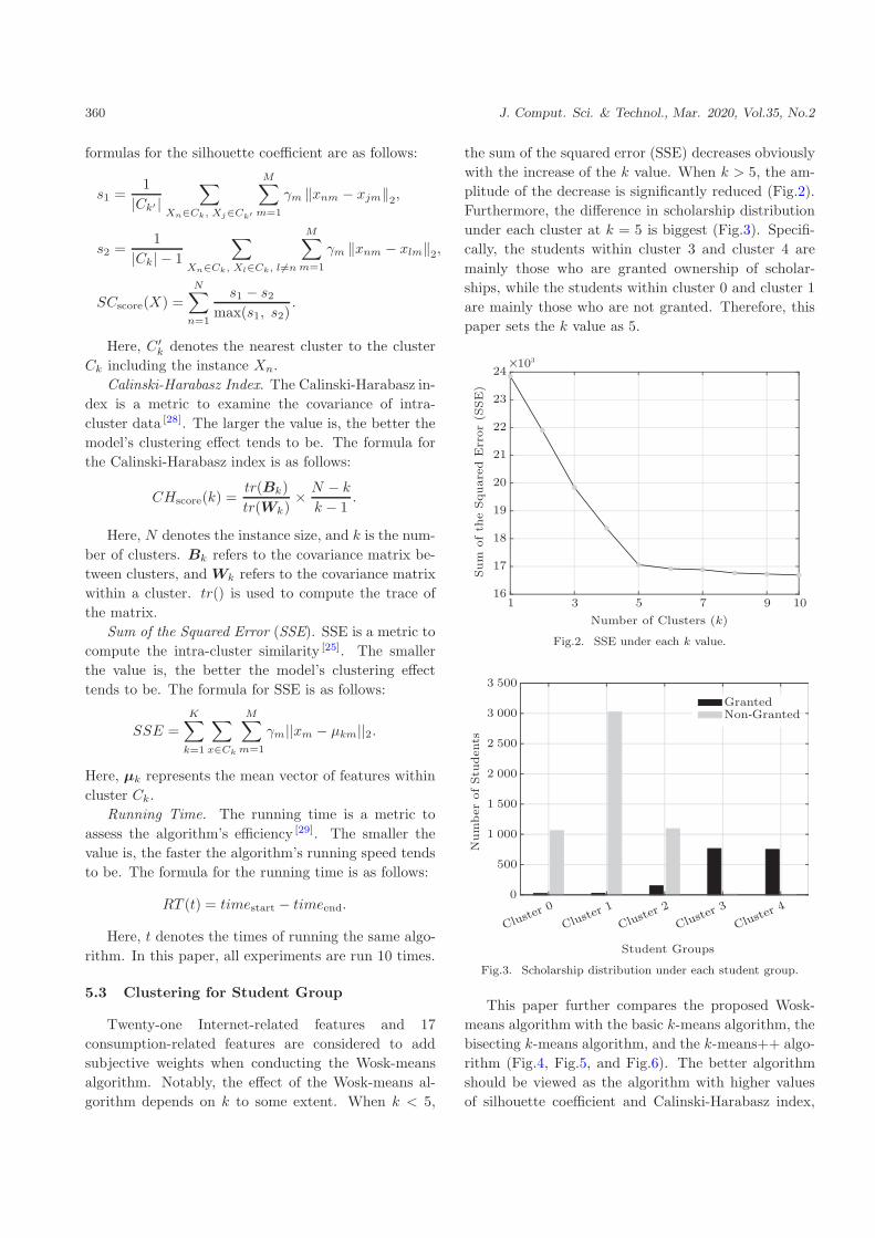
5.3 Clustering for Student Group

Twenty-one Internet-related features and 17

consumption-related features are considered to add

subjective weights when conducting the Wosk-means

algorithm. Notably, the effect of the Wosk-means al-

gorithm depends on k to some extent. When k < 5,

the sum of the squared error (SSE) decreases obviously

with the increase of the k value. When k > 5, the am-

plitude of the decrease is significantly reduced (Fig.2).

Furthermore, the difference in scholarship distribution

under each cluster at k = 5 is biggest (Fig.3). Specifi-

cally, the students within cluster 3 and cluster 4 are

mainly those who are granted ownership of scholar-

ships, while the students within cluster 0 and cluster 1

are mainly those who are not granted. Therefore, this

paper sets the k value as 5.

1 3 5 7 9 10

Number of Clusters (k)

16

17

18

19

20

21

22

23

24

Sum

of th

e S

quare

d E

rror

(SSE)

Τ103

Fig.2. SSE under each k value.

Cluster 0

Cluster 1

Cluster 2

Cluster 3

Cluster 4

Student Groups

Num

ber

of Stu

dents

0

500

1 000

1 500

2 000

2 500

3 000

3 500

GrantedNon-Granted

Fig.3. Scholarship distribution under each student group.

This paper further compares the proposed Wosk-

means algorithm with the basic k-means algorithm, the

bisecting k-means algorithm, and the k-means++ algo-

rithm (Fig.4, Fig.5, and Fig.6). The better algorithm

should be viewed as the algorithm with higher values

of silhouette coefficient and Calinski-Harabasz index,


and lower values of SSE and running time. It is obvi-

ous that the proposed algorithm outperforms the other

three algorithms in terms of most of the metrics (sil-

houette coefficient, Calinski-Harabaszindex, and SSE).

These three metrics reflect the algorithm’s intra-cluster

similarity. That is, by considering the objective weights

and subjective weights, the proposed algorithm is bet-

ter at highlighting the importance of some features.

However, the proposed algorithm is not optimal at run-

ning efficiency. As shown in Fig.7, the running time of

the Wosk-means algorithm ranks the second among the

four algorithms.

Wosk-m

eans

k-mean

s++

Bisecti

ng k-

means

k-mean

s-0.04

-0.02

0.00

0.02

Silhouett

e C

oeffic

ient

0.04

0.06

0.08

0.10

0.12

0.14

Fig.4. Comparison of silhouette coefficient with models usingthe Wosk-means algorithm and the three baseline algorithms.

0

5

10

15

20

25

30

35

40

45

Wosk-m

eans

k-mean

s++

Bisecti

ng k-

means

k-mean

s

SSE

Τ103

Fig.5. Comparison of SSE with models using the Wosk-meansalgorithm and the three baseline algorithms.

0

200

400

600

800

1 000

1 200Calinski-Harabasz IndexRunning Time (s)

Wosk-m

eans

k-mean

s++

Bisecti

ng k-

means

k-mean

s

Fig. 6. Comparisons of Calinski-Harabasz index and runningtime with models using the Wosk-means algorithm and the threebaseline algorithms.

Cluster 0

40.5% 43.6% 53.2%

44.7% 44.7%

Cluster 1 Cluster 2

Cluster 3 Cluster 4

DormitoryOthers

Fig.7. Percentage of dormitory access within each cluster.

5.4 Comparative Analysis After Clustering

Considering the above clustering analysis results,

this paper further analyzes the students’ lifestyle within

each cluster (Table 2). In terms of smart card usage,

students within cluster 4 ate breakfast most frequently,

while students within cluster 0 seldom ate breakfast.

Furthermore, the situation remains the same when

considering the detailed breakfast time slot, which con-

firms that good lifestyle habits can improve students’

academic achievement [30]. On the other hand, students

within cluster 1 and cluster 2 had a less bathing fre-

quency than the other students. In regard to canteen

consumption, the frequency of going to the canteen

among these students was not much different. In terms

of sports, students within cluster 0 and cluster 1 did

less sports, while students within cluster 2 did more

sports. Surprisingly, students within cluster 4 were the

most frequent group to go to the school hospital, and


Table 2. Students’ Lifestyle Within Each Cluster

Cluster Grant Smart Card Usage Internet Usage

Proportion Amount Breakfast Printing Canteen Bathing Sport Hospital Downlink Duration Connections

0 0.97 −97.80 −15.09 58.55 4.90 22.29 −28.71 −1.17 56.21 43.34 36.04

1 0.43 −99.42 −6.27 −28.28 −2.27 −6.05 −13.11 1.01 −9.34 −2.94 −1.25

2 8.02 −89.12 3.45 −21.71 −4.68 −37.86 18.41 −11.42 −29.17 −42.22 −45.11

3 95.41 296.45 2.90 25.15 7.90 19.90 6.94 −27.83 7.73 7.58 9.83

4 97.66 404.46 42.65 40.91 0.46 21.09 5.18 41.30 19.66 20.37 21.08

students within cluster 0 and cluster 4 preferred to go

to the printing shop. In terms of Internet usage, usage

amount and usage frequency of students within cluster

0 were both the highest, while those of students within

cluster 2 were both the lowest. Hence, students within

cluster 3 and cluster 4 had the best living habits. Al-

though students within cluster 0 had better lifestyle

habits, their breakfast habits were relatively worse and

their Internet usage amount and frequency were higher.

In addition, students within cluster 1 and cluster 2 both

had bad living habits, but the latter had a higher sports

frequency. The above analysis confirms that lifestyle

and Internet usage habits can serve as a reflection of

students’ academic achievement.

This paper also studies students’ daily habits (see

Table A1 in Appendix). First, students’ habits are

analyzed from the perspective of gender. For students

within cluster 0, cluster 1 and cluster 2, the breakfast

frequency of females was higher than that of males.

Students within cluster 3 had the opposite situation

that the female students had a lower frequency of eat-

ing breakfast. Except for students within cluster 2,

women were more likely to go to school hospitals than

men. Among students within all clusters, females had a

higher frequency of going to printing shop and bathing,

but had a lower frequency of sports and going to the

canteen than males. In terms of Internet usage, the

female students within cluster 0 had more downlink

dataflow than the male students, while the situation

for the other clusters was the opposite. The numbers

of network connections and durations of the female stu-

dents within cluster 0, cluster 1 and cluster 2 were

higher than those of the male students, and the oppo-

site was true for students within cluster 3 and cluster

4. This finding seems to be in contrast to the con-

clusion in [21] that the effect of bandwidth on males

is shown to be higher than that on females. There-

fore, further discussion should be conducted on the

relationship among gender, broadband and academic

achievement. Some similar comparative analyses have

been carried out from the perspective of disciplines and

grades, which are not stated here. It should be noted

that the values in Table A1 are the difference from the

mean.

In addition, this paper compares the differences of

research conclusions with prior studies, as shown in Ta-

ble A2 (in Appendix). The claim that good lifestyle

habits improve academic achievement remained. Al-

though females were more self-disciplined than males,

it was not sufficient to explain academic achievement.

Notably, Internet usage had a higher impact on the fe-

male students than on the male students, which was

not in line with the research of [21].

5.5 Experiments for Trajectory Deviation

After clustering analysis, this paper conducts the

deviation analysis of the trajectories. First, the stu-

dent’s access frequency of each location for each clus-

ter is recognized. This paper considers the situation

in which the length of trajectory matching is equal to

1. For each cluster, dormitory is the most frequent lo-

cation for students to access (Fig.7). Furthermore,the

matching pattern (dormitory → dormitory) far exceeds

other matching patterns within each cluster. Hence,

this paper conducts further study with the length of

the matching pattern equal to 2.

The daily trajectory is modelled to obtain a fre-

quent matching pattern of a student. To avoid infor-

mation loss, the threshold is set to 30%. That is, if the

frequency of the matching pattern exceeds 30%, it is

considered as the frequent matching pattern. Frequent

matching patterns for all students within each cluster

need to be counted subsequently. To reduce the im-

pact of uneven access frequency on different locations,

the similarity between the student trajectory and the

centroid trajectory of the cluster to which the student

belongs is further calculated based on Definition 13. Ta-

ble 3 shows the percentage of students with less than

30% similarity between the individual trajectory and


centroid trajectory within each cluster.

Table 3. Percentage of Students with Less Than 30% SimilarityBetween Individual Trajectory and Centroid Trajectory WithinEach Cluster

Cluster [0,30%) [0,20%) [0,10%)

0 6.84 3.90 1.17

1 6.78 3.85 1.18

2 5.10 2.40 0.66

3 3.89 2.84 0.41

4 5.22 4.10 1.46

The value of trajectory deviation is equal to 1 mi-

nus the trajectory similarity. Specifically, the threshold

can be adjusted to better suit different university situa-

tions. To determine the direction of the deviation, this

paper calculates the distance among these students and

each cluster. Table 4 shows the percentage of students

whose trajectory deviation is greater than the thresh-

old within each cluster (the threshold is set to 90%).

Here, the column indicates the cluster that the student

currently belongs to, and the row indicates the cluster

that the student tends to belong to. The trend that

students within cluster 0, cluster 1 and cluster 2 trans-

form to be students within cluster 3 and cluster 4 is

considered a trend worth encouraging. Moreover, the

opposite trend could be used as a basis for academic

early warning scenarios.

Table 4. Percentage of Students Whose Trajectory DeviationIs Greater Than 90% Within Each Cluster

Cluster

0 1 2 3 4

Cluster 0 – 41.67 33.33 8.33 16.67

Cluster 1 25.00 – 58.33 13.89 2.78

Cluster 2 12.50 37.50 – 50.00 0.00

Cluster 3 0.00 33.33 66.67 – 0.00

Cluster 4 10.00 20.00 40.00 30.00 –

Note: The column indicates the cluster that the student cur-rently belongs to, and the row indicates the cluster that thestudent tends to belong to.

Ultimately, the analysis results confirm that colleges

can both predict students who may receive scholarships

through their daily life habits data and apply these data

to provide decision support to help low-performing stu-

dents back on track. In terms of scholarship assign-

ment, students within cluster 3 and cluster 4 had higher

academic achievement. In detail, students within clus-

ter 4 could be regarded as the main target of large-

amount scholarships, while students within cluster 3

could be regarded as the main targets of small-amount

scholarships. The trajectory deviation analysis indi-

cates that part of students with trajectory deviations

greater than 90% show a trend of transferring to clus-

ter 3 and cluster 4. In other words, the trajectories

of these students are highly similar to those of stu-

dents with higher academic achievement. Therefore,

these students are the key targets that colleges and uni-

versities should encourage, and they can be considered

as potential recipients for small-amount scholarships to

further enhance their enthusiasm for learning. Hence,

students within cluster 0 and cluster 1 and the stu-

dents strongly tending to cluster 0 and cluster 1 could

be deemed as the targets that should be given more

attention by colleges and universities.

6 Related Work

Education data mining is the main area for explor-

ing students’ behavioural data. With the assistance of

a multi-instance multi-label algorithm, some scholars

utilized the pre-course information of each student to

predict their performance on each subsequent course [31]

and graduation failure [32]. In terms of utilization of in-

campus data, some studies have provided substantial

inspirations for this paper. For instance, Buniyamin

et al. [33] utilized campus information system data to

classify and predict student achievement. Wu et al. [13]

visualized spatial temporal features of student perfor-

mance from the activity and consumption data on cam-

pus. Hang et al. [34] explored students’ check-in be-

haviour data to predict the point-of-interest informa-

tion of college students. Guan et al. [14] and Ye et al. [15]

leveraged campus information system data to study

the assignment issues of school scholarships and grants.

Hence, this paper adopts some research ideas and meth-

ods from the above studies in exploring the factors that

influence the academic achievement of college students.

Trajectory data not only records the physical infor-

mation of a user but also reflects the personal habits

and preferences of a user to a certain extent [35]. Some

scholars have ever evaluated the similarity among users

based on GPS trajectory mining [35, 36]. It is quite diffi-

cult to obtain the GPS records of college students, and

thus, this paper generates the trajectory sequential data

for each student through in-campus behavioural data,

which is in line with these studies [14, 15]. To the best of

our knowledge, we are the first to study the problem of


identifying influencing factors of academic achievement

by utilizing students’ behavioural data.

Another related study is clustering analysis which

has been extensively applied in prior studies. In re-

gard to clustering analysis, the assignment of feature

weights is quite important, which lies in the fact that

only some features are truly valuable [23]. Huang et

al. [27] once proposed the W -k-means algorithm with-

out sacrificing the efficiency of the k-means algorithm,

which stems from the fuzzy C-means (FCM) algorithm.

Furthermore, Hung et al. [37] proposed to select the ini-

tial weight based on the coefficient of variation, thus im-

proving the performance of the W -k-means algorithm.

Abductive learning is a good framework bridging ma-

chine learning and logical reasoning [38], which can se-

lectively infer certain facts and hypotheses that explain

phenomena and observations based on known back-

ground knowledge. In this paper, domain knowledge

is taken into account when determining the weights of

features. Hence, this paper determines the weight of

features from objective and subjective perspectives to-

wards the clustering algorithm.

7 Conclusions

This paper developed a TMS approach to explore

the factors that affect the academic achievement of col-

lege students and to provide decision-making support

for early warnings. First, we segmented students into

five disjoint groups through the Wosk-means algorithm.

The behavioural factors in the clustering analysis exhib-

ited some differences from prior studies, which provide

new insights into research work in educational contexts.

Meanwhile, we analyzed manually generated trajecto-

ries data to quantify the direction of trajectory devia-

tion of students through the PrefixSpan algorithm [11].

The results could help colleges identify students who are

in need of academic warnings. We also noticed that,

bad habits and cognitive ability can reduce academic

achievement, which is the same with the prior studies

[19, 30]. Notably, female students with high academic

achievement do not show better lifestyle habits than

male students with high academic achivement that is

not completely consistent with the prior studies [12, 39].

In addition, we also viewed that, the impact of Inter-

net usage on women is stronger than on men, which is

opposite to the prior studies [21]. In the future, we will

consider the other criteria (such as course score, hon-

orary, and so on) to assess students’ academic achieve-

ment based on large-scale long-term in-campus student

data.

References

[1] Petrides K V, Frederickson N, Furnham A. The role of trait

emotional intelligence in academic performance and deviant

behavior at school. Personality and Individual Differences,

2004, 36(2): 277-293.

[2] Alloway T P, Alloway R G. Investigating the predictive roles

of working memory and IQ in academic attainment. Journal

of Experimental Child Psychology, 2010, 106(1): 20-29.

[3] Rampersaud G C, Pereira M A, Girard B L et al. Breakfast

habits, nutritional status, body weight, and academic per-

formance in children and adolescents. Journal of the Amer-

ican Dietetic Association, 2005, 105(5): 743-760.

[4] Pilcher J J, Morris D M, Donnelly J et al. Interactions

between sleep habits and self-control. Frontiers in Human

Neuroscience, 2015, 9: 284.

[5] Macan T H, Shahani C, Dipboye R L et al. College stu-

dents’ time management: Correlations with academic per-

formance and stress. Journal of Educational Psychology,

1990, 82(4): 760-768.

[6] Stadler M, Aust M, Becker N et al. Choosing between what

you want now and what you want most: Self-control ex-

plains academic achievement beyond cognitive ability. Per-

sonality and Individual Differences, 2016, 94: 168-172

[7] Lundstrom S. The impact of family income on child achieve-

ment: evidence from the earned income tax credit: Com-

ment. American Economic Review, 2017, 107(2): 623-28.

[8] Figlio D, Karbownik K, Roth J et al. School quality and

the gender gap in educational achievement. American Eco-

nomic Review, 2016, 106(5): 289-295.

[9] Jia J, Li D, Li X et al. Psychological security and deviant

peer affiliation as mediators between teacher-student rela-

tionship and adolescent Internet addiction. Computers in

Human Behavior, 2017, 73: 345-352.

[10] LeungK C. Preliminary empirical model of crucial determi-

nants of best practice for peer tutoring on academic achieve-

ment. Journal of Educational Psychology, 2015, 107(2):

558-579.

[11] Pei J, Han J, Mortazavi-Asl B et al. Prefixspan: Mining

sequential patterns efficiently by prefix-projected pattern

growth. In Proc. the 17th International Conference on Data

Engineering, April 2001, pp.215-224.

[12] Duckworth A L, Seligman M E P. Self-discipline outdoes

IQ in predicting academic performance of adolescents. Psy-

chological Science, 2005, 16(12): 939-944.

[13] Wu Y, Gong R, Cao Y et al. EduCircle: Visualizing spa-

tial temporal features of student performance from cam-

pus activity and consumption data. In Proc. International

Conference on Cooperative Design, Visualization and En-

gineering, October 2016, pp.313-321.

[14] Guan C, Lu X, Li X et al. Discovery of college students in

financial hardship. In Proc. IEEE International Conference

on Data Mining, November 2015, pp.141-150.

[15] Ye H J, Zhan D C, Li X et al. College student scholar-

ships and subsidies granting: A multi-modal multi-label ap-

proach. In Proc. the 16th IEEE International Conference

on Data Mining, December 2016, pp.559-568.


[16] Liu J, Wang D, Feng S et al. Learning distributed represen-

tations for community search using node embedding. Fron-

tiers of Computer Science, 2019, 13(2): 437-439.

[17] Zheng Y. Trajectory data mining: An overview. ACM

Trans. Intelligent Systems and Technology, 2015, 6(3): 1-

41.

[18] Singh A, Uijtdewilligen L, Twisk J W R et al. Physical

activity and performance at school: A systematic review

of the literature including a methodological quality assess-

ment. Archives of Pediatrics & Adolescent Medicine, 2012,

166(1): 49-55.

[19] Forrest C B, Bevans K B, Riley A W et al. Health and

school outcomes during children’s transition into adoles-

cence. Journal of Adolescent Health, 2013, 52(2): 186-194.

[20] Skryabin M, Zhang J J, Liu L et al. How the ICT develop-

ment level and usage influence student achievement in read-

ing, mathematics, and science. Computers & Education,

2015, 85: 49-58.

[21] Belo R, Ferreira P, Telang R. Broadband in school: Impact

on student performance. Management Science, 2013, 60(2):

265-282.

[22] Han J, Pei J, Kamber M. Data Mining: Concepts and Tech-

niques (3rd edition). Morgan Kaufmann Publishers, Mas-

sachusetts, USA, 2011.

[23] Liu H, Yu L. Toward integrating feature selection algo-

rithms for classification and clustering. IEEE Trans. Know-

ledge and Data Engineering, 2005, 17(4): 491-502.

[24] Wettschereck D, Aha D W, Mohri T. A review and em-

pirical evaluation of feature weighting methods for a class

of lazy learning algorithms. Artificial Intelligence Review,

1997, 11(1/2/3/4/5): 273-314.

[25] Tsai C Y, Chiu C C. Developing a feature weight self-

adjustment mechanism for a K-means clustering algorithm.

Computational Statistics and Data Analysis, 2008, 52(10):

4658-4672.

[26] Modha D S, Spangler W S. Feature weighting in k-means

clustering. Machine Learning, 2003, 52(3): 217-237.

[27] Huang J Z, Ng M K, Rong H et al. Automated variable

weighting in k-means type clustering. IEEE Trans. Pattern

Analysis & Machine Intelligence, 2005, 27(5): 657-668.

[28] Lord E, Willems M, Lapointe F J et al. Using the stability

of objects to determine the number of clusters in datasets.

Information Sciences, 2017, 393: 29-46.

[29] Kushnir D, Jalali S, Saniee I. Towards clustering high-

dimensional Gaussian mixture clouds in linear running

time. In Proc. the 22nd International Conference on Arti-

ficial Intelligence and Statistics, April 2019, pp.1379-1387.

[30] Basch C E. Healthier students are better learners: A miss-

ing link in school reforms to close the achievement gap.

Journal of School Health, 2011, 81(10): 593-598.

[31] Ma Y, Cui C, Nie X et al. Pre-course student performance

prediction with multi-instance multi-label learning. Science

China Information Sciences, 2019, 62(29101): 1-3.

[32] Lakkaraju H, Aguiar E, Shan C et al. A machine learn-

ing framework to identify students at risk of adverse aca-

demic outcomes. In Proc. the 21th ACM SIGKDD Int.

Conf. Knowledge Discovery and Data Mining, August 2015,

pp.1909-1918.

[33] Buniyamin N, bin Mat U, Arshad P M. Educational data

mining for prediction and classification of engineering stu-

dents’ achievement. In Proc. the 7th IEEE Int. Conf. En-

gineering Education, November 2015, pp.49-53.

[34] Hang M, Pytlarz I, Neville J. Exploring student check-in

behavior for improved point-of-interest prediction. In Proc.

the 24th ACM SIGKDD Int. Conf. Knowledge Discovery

& Data Mining, July 2018, pp.321-330.

[35] Li Q, Zheng Y, Xie X et al. Mining user similarity based

on location history. In Proc. the 16th ACM SIGSPATIAL

International Conference on Advances in Geographic In-

formation Systems, November 2008, pp.1-10.

[36] Xiao X, Zheng Y, Luo Q et al. Finding similar users using

category-based location history. In Proc. the 18th SIGSPA-

TIAL International Conference on Advances In Geographic

Information Systems, November 2010, pp.442-445.

[37] Hung W L, Chang Y C, Lee E S. Weight selection in W -

K-means algorithm with an application in color image seg-

mentation. Computers & Mathematics with Applications,

2011, 62(2): 668-676.

[38] Zhou Z H. Abductive learning: Towards bridging machine

learning and logical reasoning. Science China Information

Sciences, 2019, 62(7): 76101.

[39] Duckworth A L, Seligman M E P. Self-discipline gives girls

the edge: Gender in self-discipline, grades, and achievement

test scores. Journal of Educational Psychology, 2006, 98(1):

198-208.

Xiao-Lin Li received her Ph.D. de-

gree in computer science from the School

of Computer Science and Technology,

Jilin University, Changchun, in 2005.

She was a postdoctoral researcher of

the Department of Computer Science

and Technology of Nanjing University,

Nanjing, from 2005 to 2007. Currently

she is an associate professor in the School of Management,

Nanjing University, Nanjing. Her research interests include

data mining, business intelligence, and decision making.

She has published in refereed journals and conference

proceedings, such as TKDE, DSS, INS, KDD, AAAI. She

was on programme committees of conferences including

KDD, AAAI, IJCAI.

Li Ma currently is a Master student

of the School of Management, Nanjing

University, Nanjing. Her major re-

search interests include online customer

behaviours and data mining.text text

text text text text text text text text

text text text text text text text text


Xiang-Dong He is currently a

senior engineer of the Information

Technology Services Center, Nanjing

University, Nanjing. His current re-

search interests include smart campus,

information security and IT project

management.text text text text text

text text text text text text tex

Hui Xiong is currently a full

professor at the Rutgers, the State

University of New Jersey, where

he received the 2018 Ram Charan

Management Practice Award as the

Grand Prix winner from the Har-

vard Business Review, RBS Dean’s

Research Professorship (2016), the Rutgers University

Board of Trustees Research Fellowship for Scholarly

Excellence (2009), the ICDM Best Research Paper Award

(2011), and the IEEE ICDM Outstanding Service Award

(2017). He received his Ph.D. degree from the University

of Minnesota (UMN), Minnesota. He is a co-Editor-

in-Chief of Encyclopedia of GIS, an associate editor of

IEEE Transactions on Big Data (TBD), ACM Transac-

tions on Knowledge Discovery from Data (TKDD), and

ACM Transactions on Management Information Sys-

tems (TMIS). He has served regularly on the organiza-

tion and program committees of numerous conferences,

including as a program co-chair of the Industrial and

Government Track for the 18th ACM SIGKDD Inter-

national Conference on Knowledge Discovery and Data

Mining (KDD), a program co-chair for the IEEE 2013

International Conference on Data Mining (ICDM), a

general co-chair for the IEEE 2015 International Confe-

rence on Data Mining (ICDM), and a program co-chair

of the Research Track for the 2018 ACM SIGKDD In-

ternational Conference on Knowledge Discovery and

Data Mining. He is an IEEE Fellow and an ACM Dis-

tinguished Scientist.

Appendix

Table A1. Student Characteristics Considering Differences of Gender, Discipline and Grade

Cluster Classification Internet Usage Smart Card Usage

Downlink Dataflow Duration Connections Breakfast Printing Canteen Bathing Sport Hospital0 Female 3.05 14.76 13.95 −10.42 51.94 −5.15 39.72 −12.51 8.19

Male 0.75 3.75 6.70 −34.60 39.70 21.05 −1.80 8.95 −42.63Liberal arts 2.00 15.87 15.18 −15.41 46.79 −1.05 31.88 −17.36 4.32Science 2.49 4.74 6.76 −23.59 48.40 10.68 16.23 9.78 −27.382011 2.88 6.24 4.66 −7.54 35.73 5.26 22.25 15.75 26.012012 2.34 14.53 16.62 −26.93 57.45 3.81 26.66 −25.41 −36.18

1 Female −12.16 7.48 6.96 6.12 −19.04 −16.17 29.85 −0.57 28.28Male −7.44 −5.96 −3.78 −15.30 −49.10 1.83 −22.06 28.85 −15.91Liberal arts −15.38 4.00 4.27 2.06 −11.71 −9.02 13.50 −38.43 8.65Science −6.38 −3.85 −2.13 −12.54 −50.47 −1.99 −12.74 43.48 −5.672011 −9.95 −2.76 −1.91 3.23 −49.04 −7.22 −5.29 93.95 1.492012 −6.96 0.80 3.07 −32.14 −19.08 2.41 −4.83 13.85 −7.33

2 Female −34.52 −42.64 −45.53 20.65 −24.50 −13.45 −29.94 −39.99 −16.29Male −31.65 −45.43 −48.45 2.00 −29.03 7.55 −57.83 41.68 −11.32Liberal arts −38.95 −43.91 −47.62 −1.45 −12.26 −13.00 −39.04 −20.43 −0.80Science −27.78 −43.48 −45.63 29.00 −40.52 2.21 −42.01 1.31 −28.362011 −43.07 −51.11 −52.98 13.95 −44.67 −9.61 −45.73 23.65 −2.542012 −5.44 −21.82 −27.98 13.23 27.05 7.39 −24.75 −34.99 −48.86

3 Female 4.31 7.74 9.39 −21.80 43.90 −2.96 37.64 −40.79 −37.79Male 10.41 7.81 10.77 −10.69 1.91 14.06 7.24 −5.14 −48.16Liberal arts −0.29 6.45 9.00 −17.79 106.40 3.98 40.70 −25.53 −66.23Science 11.87 8.42 10.79 −13.99 −23.04 8.62 9.51 −29.07 −33.172011 −1.99 20.52 19.24 −41.90 −86.05 −11.18 −2.60 −14.89 −7.262012 8.14 6.87 9.60 −13.79 25.58 7.92 20.31 −63.43 −46.59

4 Female 47.11 39.28 31.68 40.34 38.53 −13.47 32.19 −20.61 46.95Male 84.99 54.09 46.39 40.44 15.35 28.12 −4.67 77.18 29.07Liberal arts 52.07 55.70 46.02 19.73 71.68 −5.08 34.76 −29.92 81.43Science 63.60 34.31 28.30 56.66 −0.12 2.33 10.30 39.43 10.112011 −7.15 −20.10 −21.53 149.31 −100.00 −24.34 −29.87 40.60 109.472012 62.24 47.65 39.60 33.17 40.84 0.88 24.34 10.07 38.77

Note: The variance of different clusters can be revealed from these numerical characteristics to some extent.


Table A2. Comparison About Research Results

Perspective Our Conclusions Behaviours in This Paper Prior Studies Comparison

LifestyleHabits

Students with higher aca-demic achievement have betterlifestyle habits

The frequency of eating break-fast, going to the canteen, sportsand bathing are higher than theaverage

Bad habits and cognitive abilitycan reduce academic achieve-ment, while good lifestylehabits can improve academicachievement [19, 30]

Consistent

Students with lower academicachievement have poorerlifestyle habits

The frequency of eating break-fast is relatively low, and the fre-quency of exercise and bathingare relatively low

For students with lower aca-demic achievement, women aremore self-disciplined than men

Women with lower academicachievement eat more frequentlythan men with lower academicachievement

Women are more self-disciplinedthan men, which explains thefemale dominance in academicachievement [12, 39]

Not completelyconsistent op-posite

For students with higher aca-demic achievement, women arenot more self-disciplined thanmen

Women with higher academicachievement do not eat more fre-quently than men with higheracademic achievement

For students with loweracademic achievement, lib-eral arts students are moreself-disciplined than sciencestudents

Liberal arts students with loweracademic achievement havehigher breakfast frequency thanscience students with loweracademic achievement

May be relatedto the genderstructure of thedepartment

LearningHabits

Students with lower academicachievement are not necessarilybad at learning habits

Some students with lower aca-demic achievement go to theprint shop frequently thanstudents with higher academicachievement

- -

InternetUsage

There is no direct correlationbetween Internet usage and aca-demic achievement

Among students who use highdataflow, duration, and connec-tions, there are some studentswith high academic achievementand some students with low aca-demic achievement

The use of Internet communicatetechnology in schools has not af-fected student performance [21]

Consistent

The impact of Internet commu-nicate technology on academicachievement has a higher im-pact on women than on men

Women with low academicachievement have higher dataflowusage, duration and connectionsthan men with low academicachievement; women with highacademic achievement have lowerdataflow usage, duration andconnections than men with highacademic achievement

Internet communicate technologyhas a higher impact on men thanon women [21]

Opposite

Spatiotemporal Representation Learning for College Student ...

Documents

Transcript of Spatiotemporal Representation Learning for College Student ...