![HiN : Alexander von Humboldt im Netz [III, 4 (2002)] - publish.UP](https://static.fdokumen.com/doc/165x107/6337acd740a96001d4010ca2/hin-alexander-von-humboldt-im-netz-iii-4-2002-publishup.jpg)
HiN : Alexander von Humboldt im Netz [III, 4 (2002)] - publish.UP
Upload
khangminh22Category
view
4download
0
Institute of Earth and Environmental Science
Spatiotemporal Variations of Key Air Pollutants
and Greenhouse Gases in the Himalayan Foothills
A cumulative dissertation for
the degree of Doctor of Natural Sciences
“doctor rerum naturalium”
(Dr. rer. Nat.) in Geoecology
Submitted to
Faculty of Mathematics and Natural Sciences
at the University of Potsdam
by
Khadak Singh Mahata
Potsdam, September 2021

Unless otherwise indicated, this work is licensed under a Creative Commons License Attribution 4.0 International. This does not apply to quoted content and works based on other permissions. To view a copy of this license visit: https://creativecommons.org/licenses/by/4.0 Submission date: 1 October 2019
Date of PhD defense: 28 June 2021
Khadak Singh Mahata: Spatiotemporal variations of key air pollutants and greenhouse gases
in the Himalayan foothills
Referees:
Prof. Dr. Mark Lawrence
University of Potsdam, Institute of Earth and Environmental Science
Managing Scientific Director, Institute for Advanced Sustainability Studies (IASS)
Germany
Prof. Dr. Juergen P. Kroop
University of Potsdam, Institute of Earth and Environmental Science
Potsdam Institute for Climate Impact Research (PIK)
Germany
Prof. Nguyen Thi Kim Oanh
Asian Institute of Technology, Department of Energy, Environment and Climate, Scholl of
Environment, Resources and Development
Thailand
Published online on the Publication Server of the University of Potsdam: https://doi.org/10.25932/publishup-51991 https://nbn-resolving.org/urn:nbn:de:kobv:517-opus4-519910


i
Abstract
South Asia is a rapidly developing, densely populated and highly polluted region that is facing
the impacts of increasing air pollution and climate change, and yet it remains one of the least
studied regions of the world scientifically. In recognition of this situation, this thesis focuses
on studying (i) the spatial and temporal variation of key greenhouse gases (CO2 and CH4) and
air pollutants (CO and O3) and (ii) the vertical distribution of air pollutants (PM, BC) in the
foothills of the Himalaya. Five sites were selected in the Kathmandu Valley, the capital region
of Nepal, along with two sites outside of the valley in the Makawanpur and Kaski districts, and
conducted measurements during the period of 2013-2014 and 2016. These measurements are
analyzed in this thesis.
The CO measurements at multiple sites in the Kathmandu Valley showed a clear diurnal cycle:
morning and evening levels were high, with an afternoon dip. There are slight differences in
the diurnal cycles of CO2 and CH4, with the CO2 and CH4 mixing ratios increasing after the
afternoon dip, until the morning peak the next day. The mixing layer height (MLH) of the
nocturnal stable layer is relatively constant (~ 200 m) during the night, after which it transitions
to a convective mixing layer during the day and the MLH increases up to 1200 m in the
afternoon. Pollutants are thus largely trapped in the valley from the evening until sunrise the
following day, and the concentration of pollutants increases due to emissions during the night.
During afternoon, the pollutants are diluted due to the circulation by the valley winds after the
break-up of the mixing layer. The major emission sources of GHGs and air pollutants in the
valley are transport sector, residential cooking, brick kilns, trash burning, and agro-residue
burning. Brick industries are influential in the winter and pre-monsoon season. The
contribution of regional forest fires and agro-residue burning are seen during the pre-monsoon
season. In addition, relatively higher CO values were also observed at the valley outskirts
(Bhimdhunga and Naikhandi), which indicates the contribution of regional emission sources.
This was also supported by the presence of higher concentrations of O3 during the pre-monsoon
season.
The mixing ratios of CO2 (419.3 ±6.0 ppm) and CH4 (2.192 ±0.066 ppm) in the valley were
much higher than at background sites, including the Mauna Loa observatory (CO2: 396.8 ± 2.0
ppm, CH4:1.831 ± 0.110 ppm) and Waligaun (CO2: 397.7 ± 3.6 ppm, CH4: 1.879 ± 0.009 ppm),
China, as well as at an urban site Shadnagar (CH4: 1.92 ± 0.07 ppm) in India.

ii
The daily 8 hour maximum O3 average in the Kathmandu Valley exceeds the WHO
recommended value during more than 80% of the days during the pre-monsoon period, which
represents a significant risk for human health and ecosystems in the region. Moreover, in the
measurements of the vertical distribution of particulate matter, which were made using an
ultralight aircraft, and are the first of their kind in the region, an elevated polluted layer at
around ca. 3000 m asl. was detected over the Pokhara Valley. The layer could be associated
with the large-scale regional transport of pollution. These contributions towards understanding
the distributions of key air pollutants and their main sources will provide helpful information
for developing management plans and policies to help reduce the risks for the millions of
people living in the region.

iii
Zusammenfassung
Südasien ist eine sich schnell entwickelnde, dicht besiedelte und stark umweltbelastete Region,
die mit den Auswirkungen der zunehmenden Luftverschmutzung und des Klimawandels
konfrontiert ist, und dennoch bleibt sie wissenschaftlich gesehen eine der am wenigsten
untersuchten Regionen der Welt. In Anerkennung dieser Situation liegt der Schwerpunkt dieser
Arbeit auf der Untersuchung (i) der räumlichen und zeitlichen Variation der wichtigsten
Treibhausgase (CO2 und CH4) und Luftschadstoffe (CO und O3) und (ii) der vertikalen
Verteilung der Luftverschmutzung (PM, BC) in den Vorgebirgen des Himalayas. Fünf
Standorte wurden im Kathmandu-Tal, der Hauptstadtregion Nepals, sowie zwei Standorte
außerhalb des Tals in den Distrikten Makawanpur und Kaski ausgewählt und im Zeitraum
2013-2014 und 2016 wurden Messungen durchgeführt. Diese Messungen werden in dieser
Arbeit analysiert.
Die CO-Messungen an mehreren Standorten im Kathmandu-Tal zeigten einen klaren
Tagesablauf: Die Werte am Morgen und am Abend waren hoch, mit einem Rückgang am
Nachmittag. Es gibt leichte Unterschiede in den Tageszyklen von CO2 und CH4, wobei die
Mischungsverhältnisse von CO2 und CH4 nach dem Nachmittagsdip bis zu den höchsten
Werten am nächsten Morgen zunehmen. Die Höhe der nächtlichen stabilen planetaren
Grenzschicht ist relativ konstant (~ 200 m), danach geht sie tagsüber in eine konvektive
Mischschicht über und die MLH ("Mixing layer height") steigt am Nachmittag auf bis zu 1400
m an. So werden Schadstoffe vom Abend bis zum Sonnenaufgang des folgenden Tages
weitgehend im Tal gefangen, und die Schadstoffkonzentration steigt durch nächtliche
Emissionen an. Während des Nachmittags werden die Schadstoffe aufgrund der Zirkulation
durch die Talwinde nach dem Aufbrechen der Mischschicht verdünnt. Die
Hauptemissionsquellen für GHGs und Luftschadstoffe im Tal sind der Verkehrssektor, das
Kochen in privaten Haushalten, Ziegeleien, die Müllverbrennung und die Verbrennung von
landwirtschaftlichen Reststoffen. Die Ziegelindustrie ist in der Winter- und Vormonsunzeit
von großer Bedeutung für die Emissionen von Ruß. Der Beitrag der regionalen Waldbrände
und der Verbrennung von landwirtschaftlichen Reststoffen ist besonders wichtig in der
Vormonsunzeit. Darüber hinaus wurden auch am Talrand (Bhimdhunga und Naikhandi) relativ
hohe CO-Werte beobachtet, was auf den Beitrag der regionalen Emissionsquellen hinweist.
iv
Dies wurde auch durch das Vorhandensein höherer Konzentrationen von O3 während der
Vormonsunzeit unterstützt.
Die Mischungsverhältnisse von CO2 (419,3 ±6,0 ppmv) und CH4 (2.192 ±0,066 ppmv) im Tal
waren viel höher als an bekannten Hintergrundstandorten, darunter das Observatorium Mauna
Loa (CO2: 396,8 ± 2,0 ppmv, CH4:1.831 ± 0,110 ppmv) und Waligaun (CO2: 397,7 ± 3,6 ppmv,
CH4: 1,879 ± 0,009 ppmv), China, sowie an einem städtischen Standort Shadnagar (CH4: 1,92
± 0,07 ppmv) in Indien.
Der tägliche 8-stündige maximale O3-Durchschnitt im Kathmandu-Tal übersteigt den WHO-
Empfehlungswert an mehr als 80% der Tage während der Vormonsunzeit, was ein erhebliches
Risiko für die menschliche Gesundheit und die Ökosysteme in der Region darstellt. Darüber
hinaus wurde bei den Messungen der vertikalen Verteilung der Feinstaubpartikel, die mit
einem Ultraleichtflugzeug durchgeführt wurden und die ersten ihrer Art in der Region sind,
eine höherliegende verschmutzte Schicht, ca. 3000 m über dem mittleren Meeresspiegel über
dem Pokhara-Tal, festgestellt. Die Schicht könnte mit dem großräumigen regionalen Transport
von Schadstoffen in Verbindung gebracht werden. Diese Beiträge zum Verständnis der
Verteilung der wichtigsten Luftschadstoffe und ihrer Hauptquellen werden hilfreiche
Informationen für die Entwicklung von Mitigationsplänen und -strategien liefern, die dazu
beitragen, die Risiken für die Millionen von Menschen, die in der Region leben, zu verringern.

v

vi
Acknowledgement
I would like to acknowledge some notable persons and organizations who helped me in
different ways to bring out this thesis.
First of all, I would like to thank my supervisor Prof. Dr. Mark G. Lawrence for providing me
an opportunity to work with him as a junior fellow at IASS, Germany and accepting me as a
PhD scholar as well as for his guidance to complete the thesis and papers. I am grateful to my
mentor Dr. Maheswar Rupakheti at IASS for his timely advice and guidance. I am also grateful
to Dr. Arnico K. Panday at ICIMOD, Nepal for his continuous support and guidance.
I am thankful to IASS which provided me the fellowship to complete the doctoral degree as
well as funding for the research work. Similarly, I would also like to thank my PhD advisory
committee (PAC) members Prof. Peter Builtjes and Prof. Tim Butler for their guidance, and
colleagues at IASS Dr.Ashish Singh, Dr. Andrea Mues, Dr. Pankaj Sadavarte, Dr. P. S.
Praveen, Dr. Noelia Otero Felipe, Tanja Baines, Iris Schuetze, Cordula Granderath who
supported me during my doctoral degree.
I would like to thank ICIMOD for helping in technical and logistic support during the SusKat-
ABC campaign in Nepal as a collaborating partner.
I would also like to thank Shyam Newar, Bhogendra Kathayat, Dipesh Rupakheti and Raviram
Pokharel who helped me during SusKat-ABC campaign.
Lastly, I would express my deep gratitude to my parents, my brother, Tika Ram Mahata, my
friend, Dr. Naresh Neupane and my wife, Bhumika Mahata.

vii

viii
Table of Contents
Abstract ................................................................................................................................... i
Zusammenfassung .................................................................................................................iii
Acknowledgement ................................................................................................................. vi
Table of Contents ................................................................................................................viii
List of Figures ........................................................................................................................ x
List of Tables ....................................................................................................................... xii
Abbreviations and Symbols ................................................................................................. xiv
Chapter 1 .................................................................................................................................... 1
1.1. Motivation of the study............................................................................................ 4
1.2. Set up, site selection and methods ........................................................................... 5
1.3. Hypothesis, key research questions and organization of the thesis ......................... 6
1.4. Key results of the three studies .............................................................................. 10
1.4.1. CH4 and CO2 in the region ................................................................................. 10
1.4.2. Air pollutants (CO and O3) at multiple sites in the Kathmandu Valley............. 11
1.4.3. Vertical distribution of air pollutants ................................................................. 12
1.5. Further contributions ............................................................................................. 12
Chapter 2 .................................................................................................................................. 14
Abstract .................................................................................................................................... 14
2.1. Introduction ........................................................................................................... 15
2.2. Experiment and Methodology ............................................................................... 18
2.2.1. Kathmandu Valley ............................................................................................. 18
2.2.2. Study sites .......................................................................................................... 20
2.2.2.1. Bode (SusKat-ABC supersite) .................................................................... 20
2.2.2.2. Chanban ...................................................................................................... 20
2.2.3. Instrumentation .................................................................................................. 21
2.3. Results and discussion ........................................................................................... 24
2.3.1. Time series of CH4, CO2, CO and water vapor mixing ratios ........................... 24
2.3.2. Monthly and seasonal variations ........................................................................ 28
2.3.3. Diurnal variation ................................................................................................ 35
2.3.4. Seasonal interrelation of CO2, CH4 and CO ...................................................... 40
2.3.5. CO and CO2 ratio: Potential emission sources .................................................. 40
2.3.6. Comparison of CH4 and CO2 at semi-urban site (Bode) and rural site
(Chanban) ........................................................................................................... 44
2.4 Conclusions ........................................................................................................... 47
Chapter 3 .................................................................................................................................. 50

ix
Abstract .................................................................................................................................... 50
3.1 Introduction ........................................................................................................... 51
3.2 Study sites and methods ........................................................................................ 55
3.3 Results and discussion ........................................................................................... 60
3.3.1 CO mixing ratio at multiple sites ....................................................................... 60
3.3.2 Diurnal and seasonal variations of CO .............................................................. 61
3.3.2.1 Diurnal pattern of CO at multiple sites ....................................................... 61
3.3.2.2 CO diurnal variation across seasons ........................................................... 64
3.3.2.3 Regional influence on CO in the valley...................................................... 66
3.3.3 O3 in the Kathmandu Valley and surrounding areas .......................................... 68
3.3.4 O3 seasonal and diurnal variation ...................................................................... 72
3.3.5 CO emission flux estimate ................................................................................. 74
3.4 Conclusions ........................................................................................................... 79
Chapter 4 .................................................................................................................................. 81
4 An Overview on the Airborne Measurement in Nepal, - Part 1: Vertical Profile of
Aerosol Size-Number, Spectral Absorption, and Meteorology ....................................... 81
Abstract ............................................................................................................................ 81
4.1 Introduction ........................................................................................................... 82
4.2 Ultralight measurements in Nepal ......................................................................... 84
4.2.1 Details of the airborne measurement unit .......................................................... 84
4.2.2 Site description................................................................................................... 86
4.2.3 Test flight patterns over the Pokhara Valley...................................................... 86
4.2.4 Data processing and quality ............................................................................... 87
4.3 Results ................................................................................................................... 88
4.3.1 General meteorology and air quality, aerosol properties in the Pokhara Valley 88
4.3.1.1 Local and synoptic meteorology in the Pokhara Valley ............................. 88
4.3.1.2 Overview of the aerosol properties in the Pokhara Valley during the test flight
period ............................................................................................................... 90
4.3.2 Vertical profiles of absorbing aerosols, particle number and size distribution,
temperature, and dew point ................................................................................ 91
4.3.3 Diurnal variation in the vertical profiles ............................................................ 93
4.3.4 Nature of absorbing aerosols in the Pokhara Valley .......................................... 94
4.3.5 Comparison of the satellite-derived vertical profiles with measurements ......... 96
4.3.6 Role of synoptic circulation in modulating aerosol properties over the Pokhara
Valley ................................................................................................................. 97
4.4 Conclusion ............................................................................................................. 99
Chapter 5 ................................................................................................................................ 101
5 Discussion and Conclusions .......................................................................................... 101

x
5.1 Overview and key messages ................................................................................ 101
5.2 Conclusions and future priorities ......................................................................... 105
Bibliography .......................................................................................................................... 127
Declaration of Authorship ................................................................................................. 144
List of Figures
2.1. Location of the measurement sites and general setting of a supersite Bode ..................... 22
2.2. Time series of hourly average mixing ratios of CH4, CO2, CO, and water vapor and
temperature and rainfall at Bode. ..................................................................................... 25
2.3. Monthly variations of the mixing ratios of hourly CH4, CO2, CO, and water vapor
observed at Bode in the Kathmandu Valley ..................................................................... 28
2.4. Relation between mixing ratios of CH4, CO2, CO and wind direction observed at Bode in
the Kathmandu Valley from March 2013 to February 2014 ............................................ 33
2.5. Satellite detected fire counts in Mar, Apr, May 2013 in the broader region surrounding
Nepal and total number of fire counts detected by MODIS during Jan 2013-Feb 2014 .. 34
2.6. Diurnal variations of CH4, CO2, CO, and water vapor in different seasons observed at
Bode in the Kathmandu Valley ........................................................................................ 36
2.7. Diurnal variations of hourly mixing ratios of CH4, CO2, CO, and mixing layer height
(MLH) at Bode in different seasons ................................................................................. 39
2.8. Seasonal polar plot of hourly dCO/dCO2 ratio based upon wind direction and wind speed
.......................................................................................................................................... 43
2.9. Seasonal frequency distribution of hourly dCO/dCO2 ratio during morning hours and
evening hours ................................................................................................................... 44
2.10. Comparison of hourly average mixing rations of CH4, CO2, CO, and water vapor
observed at Bode and Chanban. ....................................................................................... 45
2.11. Diurnal variations of hourly average mixing ratios of CH4, CO2, CO and water vapor
observed at Bode and Chanban ........................................................................................ 46
3.1. Observation sites in the SusKat-ABC international air pollution campaign during 2013-
2014 in the Kathmandu Valley ......................................................................................... 57
3.2. Hourly average CO mixing ratios observed at a supersite (Bode) and three satellite sites
(Bhimdhunga, Naikhandi and Nagarkot) ......................................................................... 60
3.3. Diurnal variations of CO mixing ratios during the common observation period (13
February–03 April, 2013) at Bode, Bhimdhunga, Naikhandi and Nagarkot ................... 62
3.4. Comparison of seasonal diurnal variation of hourly average CO mixing ratios at Bode,
Bhimdhunga and Naikhandi ............................................................................................. 64
3.5. Comparison of hourly average CO mixing ratios during normal days and episode days in
2013 at Bode, Bhimdhunga and Naikhandi in the Kathmandu Valley ............................ 67

xi
3. 6. Time series of hourly average and daily maximum 8-hr average O3 mixing ratio at
Bode, Paknajol, Nagarkot and Pulchowk ......................................................................... 69
3.7. Seasonal diurnal pattern of hourly average O3 mixing ratio during January 2013-January
2014 at Bode, Paknajol, and Nagarkot ............................................................................. 73
3. 8. Monthly CO emission flux based on the mean diurnal cycle of CO mixing ratios with all
days (CO Flux) and with only morning hours data (CO Flux minimum). ....................... 77
4.1. A typical test flight within the Pokhara Valley on 5 May 2016 ....................................... 87
4.2. Daily wind vector data at 850 and 500 mb, plotted using the NCEP NCAR reanalysis
(2.5° x 2.5°) data over South Asia from 1-7 May 2016 ................................................... 89
4.3. AOD and other data products from the Level1.5 AERONET direct product in the
Pokhara Valley from 1-10 May 2016. .............................................................................. 90
4.4. Vertical profiles of aerosol species and meteorological parameters during the 5-7 May
2016 test flights in the Pokhara Valley using the IKARUS microlight aircraft ............... 92
4.5. Aerosol extinction coefficient (at 532 nm) vertical profile and aerosol type classification
based on the CALIPSO level 2 retrieval .......................................................................... 95
4.6. YSPLIT 3 day back trajectories of air masses arriving at 3 different heights (800 m,
1500 m and 2500 m) from above the ground level in the Pokhara Valley.. ..................... 96
A.1. Correlation between hourly Picarro and Horriba CO mixing ratios at Bode during 6
March to 7 June 2013 in the Kathmandu Valley..................................................... 107
A.2. Seasonal diurnal variation of hourly average wind directions at Bode.......................... 108
A.3. Seasonal diurnal variation of hourly average wind speeds at Bode. .............................. 109
A.4. Time series of hourly average ambient temperature, wind speed, pressure, and rainfall
observed at Chanban site in Makwanpur district ........................................................... 110
B.1. Testing and assembly of the instrument package inside IKARUS-C42, field station in
Pokhara Valley and sketch of the Instrument package ................................................... 111
B.2. Monthly mean values of key meteorological parameters at the Pokhara regional airport
........................................................................................................................................ 112
B.3. Frequency of wind speed and direction observed in the Pokhara Valley during May
2016 ................................................................................................................................ 113
B.4. Daily temperature and relative humidity at 500mb using the NCEP NCAR reanalysis
(2.5x 2.5o) data over South Asia from May 1 to 7 2016. ............................................... 114
B.5. Monthly mean value of AOD 500 nm in Pokhara Valley for 2010-2016 ...................... 115
B.6. Local Meteorology in the Pokhara Valley from 1-10 May 2016. .................................. 116
B.7. AERONET-based aerosol optical depth and radiative properties in the Pokhara Valley
from 2010 to 2016. ......................................................................................................... 120
B.8. MODIA AQUA AND TERRA AOD at 550 nm over the IGP and Himalayan region
from 1 – 7 May .............................................................................................................. 122

xii
B.9. Locally or nationally recorded active fire for the same period by the National
Emergency Operation Centre ......................................................................................... 123
B.10. Morning test flight (Flight F3) on 6 May 2016 ............................................................ 124
B.11. Estimating the AAE value using the power fit and linear fit. ...................................... 125
List of Tables
2.1. Instruments and sampling at Bode and Chanban sites ...................................................... 21
2.2. Summary of monthly average CH4 and CO2 mixing ratios observed at Bode in the
Kathmandu Valley during March 2013 to Feb 2014 ........................................................ 27
2.3. Summary of CH4 and CO2 mixing ratios at Bode across four seasons during March 2013
to Feb 2014 ....................................................................................................................... 29
2.4. Comparison of monthly average CH4 and CO2 mixing ratios at Bode and Chanban sites
in Nepal with other urban and background sites in the region ......................................... 30
2.5. Emission ratio of CO/CO2 (ppb ppm-1) derived from emission factors .......................... 41
2.6 Average of the ratio of dCO to dCO2, their Geometric mean over a period of 3 hours
during morning peak, evening peak and seasonal of the ambient mixing ratios of CO and
CO2 and their lower and upper bound. ............................................................................ 44
3.1 Information of the sampling sites of the SusKat-ABC campaign during 2013-2014 in the
Kathmandu Valley. ........................................................................................................... 56
3.2. Details of the instruments deployed at different sites during the observation period during
January 2013-March 2014 in the Kathmandu Valley. ..................................................... 58
3.3. Summary of the monthly average ozone mixing ratios (ppb) at four sites in the
Kathmandu Valley, Nepal; and two sites (Manora Peak and Delhi) in India. ................. 70
3.4. verege CO mixing ratio at different time of the day (daytime and nighttime) and the
monthly average (total) at four sites in the Kathmandu Valley ....................................... 70
T.1 …………………………………………………………………………………………126

xiii

xiv
Abbreviations and Symbols
AGL : Above Ground Level
AOD : Aerosol Optical Depth
ASL : Above Sea Level
AWS : Automatic Weather Station
BC : Black Carbon
CBS : Central Bureau of Statistics
CO : Carbon Monoxide
CO2 : Carbon Dioxide
CH4 : Methane
GBD : Global Burden of Disease
GoN : Government of Nepal
GHG : Greenhouse Gas
HKH : Hind Kush Himalaya
IASS : Institute for Advanced Sustainability Studies
ICIMOD : International Centre for Integrated Mountain Development
IGP : Indo-Gangetic Plain
INTEX-B : Intercontinental Chemical Transport Experiment - Phase B
IPCC : Intergovernmental Panel on Climate Change
MLH : Mixing Layer Height
MOPITT : Measurements of Pollution in the Troposphere
NOx : Nitrogen dioxides
O3 : Ozone
OC : Organic Carbon
PM : Particulate Matter

xv
REAS : Regional Emission Inventory in Asia
RCP : Representative Concentration Pathways
SLCPs : Short-Lived Climate-forcing Pollutants
SO2 : Sulphur Dioxide
SusKat-ABC : Sustainable Atmosphere for the Kathmandu Valley – Atmospheric
Brown Clouds
TP : Tibetan Plateau
VOCs : Volatile Organic Compounds
WHO : World Health Organization


1
Chapter 1
Introduction and Overview
Climate change and air pollution are closely interlinked challenges for human societies and
ecosystems (IPCC 2013). Both air pollution and climate change are adversely impacting public
health, crops, weather and climate, as well as global ecosystems, which ultimately affects the
livelihood of the people, environment, economies and sustainable development of societies.
This worsening situation needs effective policies to limit anthropogenic emissions of air
pollutants, including short-lived climate-forcing pollutants (SLCPs), as well as greenhouse
gases (GHGs). Sources of these anthropogenic emissions are mainly industries, the energy
sector, the transport sector, household cooking, biomass burning (including agro-residue
burning) and land-use change (deforestation). While the emissions from several of these sectors
are going down in developed countries due to effective implementation of environmental
protection laws, they are instead mostly increasing in developing and under-developed nations,
such as in South Asia, due to either non-existent or ineffective protection measures.
Local emission sources (for example, transport, residential, and industrial activities) are not
only responsible for degrading air quality, but they are also playing significant role in the
increasing atmospheric mixing ratios of GHGs in South Asia, including in the central
Himalayan mountain region. The regional scale air pollution (now called atmospheric brown
clouds, ABC) in South Asia has come into the spotlight after the findings of the INDOEX field
campaign during 1999, in which it was found that ABCs extend vertically to several kilometers
above the ground, with sometimes elevated layers found at an altitude of ca. 3000 m asl.
(Ramanathan et al., 2001). Furthermore, air pollution is found to be responsible for over a
million pre-mature deaths annually in the southern Asian region. Several studies have
examined how such sources and pollutants are major contributors to the ever-deteriorating air
quality in the region (Panday and Prinn, 2009; Putero et al., 2014; Sinha et al., 2014; Marinoni
et al., 2013). In order to develop effective mitigation strategies, it is important to understand
the influence of regional emission sources on the various air pollutants and their horizontal and
vertical distributions in the region.

Chapter 1. Introduction and overview
2
The effects of air pollution on human health have become recognized as being very significant
(WHO 2014; UNEP/WMO 2011), with an estimated 8 million premature deaths annually
around the world, especially in less-developed regions, with ~ 90% of the premature deaths in
low and middle income nations (https://www.who.int/airpollution/en/). The effects are
particularly bad in South Asia in comparison to other parts of the World (Forouzanfar, 2015).
In Nepal, a small country in the central Himalayas, air pollution (both outdoor and indoor) has
become the most significant environmental health risk, responsible for about 45305 premature
death in 2016 (WHO 2018). In addition, the damage to ecosystems, including agriculture, is
also immense. For example, worldwide reductions in crop yields due to high levels of
tropospheric ozone (O3) were estimated to be $11-18 billion in 2000 (Avnery et al., 2011;
UNEP and WMO 2011). Crop damage is also particularly bad in developing regions like South
Asia; for example, in India alone the wheat loss mainly due to O3 was equivalent to $5 billion
in 2010 (Burney and Ramanathan, 2014).
Tropospheric O3 is not only detrimental to human health, ecosystem and crop productivity
(Monks et al., 2015; WHO, 2003), but it is also a greenhouse gas. A recent study reported that
the levels of O3 are decreasing in western Europe and North America, while they have been
increasing in East Asia during the period of 2000 to 2014 (Chang et al., 2017), and could not
be reported on reliably for South Asia because of the lack of monitoring stations, although
South Asia is expected to become one of the global hotspots for O3 pollution by 2030 (IEA
2016; Dentener et al., 2006). In South Asia, O3 levels are observed to be high during the pre-
monsoon season (March-May) (Bhardwaj et al., 2018; Putero et al., 2015; Gouda et al., 2014;
Lawrence and Lelieveld, 2010; Pudasainee et al., 2006), because of the high temperature and
solar insolation coupled with urban precursors along with an increase in forest fires and agro-
residue burning compared to other seasons (Putero et al., 2015; Kumar et al., 2011; Dev Roy
et al., 2009). There are several other important pollutants in urban environments, including the
main precursors of O3: nitrogen oxides (NOx), carbon monoxide (CO), methane (CH4) and
volatile organic compounds (VOCs). Among these, CO is a toxic gas and has direct and indirect
impacts on health and the environment (Raub et al., 2000; White et al., 1989). It is emitted
from incomplete combustion of biomass and fossil fuels. Urban areas normally have a large
number of industries and vehicles which emit CO. CO is a useful indicator for monitoring
urban air pollution because of having similar combustion sources to particulates and other
primary pollutants. Because of its 4-8 weeks tropospheric lifetime, it is also considered to be a
good indicator of regional (and/or intercontinental) pollution transport (Yashiro et al., 2009).

Chapter 1. Introduction and overview
3
CO does not have a direct impact on the climate (it is not a greenhouse gas), but it contributes
considerably to O3 production in urban areas.
Beyond tropospheric O3, the most important GHGs are CO2 and CH4 (Stevenson et al., 2013;
Xu et al., 2016; IPCC, 2013; Ramanathan and Carmichael, 2008; IPCC, 2007). CO2 and CH4
are relatively non-reactive gases and are thus relatively long-lived and well-mixed in the
troposphere. Their mixing ratios have risen by 40% and 150%, respectively, since the
beginning of the industrial age to 2011 (IPCC, 2013), contributing significantly to the projected
increase in global average temperature exceeding 2 °C by the end of 21st century (IPCC, 2013).
In addition to industrial, energy and mobility sector process, land use changes, especially due
to rapid urbanization and deforestation to create agricultural lands, are also responsible for the
increasing mixing ratios of these species in the atmosphere. Asia is one of the global hotspots
for CH4 emissions, due to livestock farming, cultivation of soils and especially of rice beds,
coal extraction, ineffective waste disposal, etc. (EDGAR2FT, 2013). South Asia contributed
nearly 40 Tg annually to CH4 emissions, or about 8 % of total global emissions (500 Tg) in the
2000s (Patra et al., 2013).
Especially the Hindu Kush-Himalayan (HKH) region of South Asia, which is rich in
biodiversity and water resources, is highly vulnerable to the impacts of climate change and air
pollution, as evident in many ways. However, South Asia in general is a relatively poorly
studied region. Developing reliable estimates of emissions and their contribution to pollution
levels and global warming is made complicated by the fact that the majority of the people in
the region still depend on solid fuels (wood, dung, charcoal, coal) for household cooking and
heating (UNEP, 2018), and the GDP of most countries in South Asia is based on agriculture
(CBS, 2011; Pandey et al., 2014). Most of the energy required for the economic development
is generated from low grade coal thermal plants and low-quality fossil fuels for the transport
and industrial sectors. Because of the low per capita income and often corrupt bureaucracy, it
is hard to implement effective policies to curb air pollution. Thus, most of the transport sector,
agriculture and energy sectors still use inefficient technologies, often without filters for
controlling air pollutants, and burn low grade fuels. Better knowledge of the levels and sources
of various pollutants and greenhouse gases is needed in order to help policymakers and the
broader public aware of the issue of air pollution and climate change, in order to support
effective mitigation actions. However, developing this knowledge for this region is
significantly hindered by the lack of high-quality observations, including intensive field
measurements and longer-term monitoring stations, as well as information on the spatial and

Chapter 1. Introduction and overview
4
temporal distributions of air pollutants and GHGs and their relationship to the regional
meteorological parameters. Establishing this would be useful for policymakers in developing
science-informed mitigation plans. As described in the following sections, this thesis
contributes s an important contribution to improving the understanding characteristics of key
air pollutants and greenhouse gases and their sources in this vulnerable region.
1.1. Motivation of the study
Nepal is situated in the central Himalayas, and its highly populated Kathmandu Valley is
located at the foothills of the Himalaya, midway between the Indo-Gangetic Plain (IGP) and
Tibetan Plateau (TP), and is highly vulnerable to air pollution and climate change. However,
the government of Nepal (GoN) has only limited research results available on air quality and
climate change, due to lack of research and resources. Although GoN has recently started
setting up air quality monitoring stations in Nepal, including few sites in and around the
Kathmandu Valley and other regions such as the Pokhara Valley to the west of Kathmandu,
the number of stations is not yet sufficient to provide an adequate picture of the state of air
quality throughout the country with complex topography. Thus, further scientific studies of the
regional air quality and climate change are necessary to understand major air pollutants and
greenhouse gases, their sources (local and regional), their temporal and spatial (both horizontal
and vertical) distributions in the atmosphere, their potential impacts on human health and
ecosystems, and the implications for socio-economic development, as a basis for designing
appropriate mitigation measures.
Associated with the diverse physical topography and landscape of Nepal, numerous valleys
and gorges act as pathways for the transport of polluted air masses from the IGP to the TP
(Dhungel et al., 2018; Lüthi et al., 2016; Putero et al., 2015; Bonasoni et al., 2010).
Furthermore, recent studies have shown that the pollution from the IGP region, along with
regional forest fires and agro-residue burning, influence the air pollution in this region,
including the high Himalayas and the TP (Bhardwaj et al., 2018; Mahata et al., 2018; Li et al.,
2017; Rupakheti et al., 2017; Putero et al., 2015; Sinha et al., 2014; Marinoni et al., 2013;
Bonasoni et al., 2010). Many of the transported air pollutants, such as O3, CO, and also
components of particulate matter (PM) such as black carbon (BC) aerosol particles cause
heating of the lower atmosphere and surface, which influences the Indian monsoon circulation
(Ramanathan et al, 2001; 2005). Similarly, BC and mineral dust deposit on the snow and
glaciers, and their light-absorbing components accelerate glacier retreat, which affects billions

Chapter 1. Introduction and overview
5
of people in the region (Wester, 2019; UNEP, 2018; Li et al., 2017; Li et al., 2016). Improving
knowledge of air pollution and climate change, as well as the sources of air pollutants and
GHGs in the Himalayan-Tibetan mountain and foothill regions, will require well-placed and
high-quality observations of atmospheric constituents, as well as a quantitative, spatiotemporal
analysis of air pollutants and GHGs in the region.
1.2. Set up, site selection and methods
The international air pollution measurement campaign “Sustainable Atmosphere for the
Kathmandu Valley-Atmospheric Brown Clouds (SusKat-ABC)” was conducted from
December 2012 to June 2013 (with some of the measurements being continued for more than
a year beyond that). SusKat-ABC campaign was led by the Institute for Advanced
Sustainability Studies (IASS), Germany, in collaboration with the International Centre for
Integrated Mountain Development (ICIMOD), Nepal. In addition, 18 research groups from 9
countries joined in to make additional measurements during the campaign. Simultaneous
measurements of various air pollutants and GHGs were carried out at 6 sites in the Kathmandu
Valley and several regional sites in Nepal (Lumbini, Pokhara, Jomsom, Dhunche and the
“Pyramid” station at the base camp of Mt. Everest), as well as in India (Nainital, Pantanagar
and Mohali) and China (Nam Co station and the Everest station) (Rupakheti et al., 2019, in
preparation). More than 40 papers based on the SusKat-ABC campaign have been published
or are under review. This thesis is based on three published peer-reviewed papers that focus on
the seasonal and diurnal variation of GHGs and air pollutants, the spatial distribution of air
pollutants, an emission flux estimation for carbon monoxide, and the vertical distribution of
aerosol particles and the extent of their regional transport in the foothills of the Himalaya. The
studies included in this thesis were conducted mainly in the Kathmandu Valley and the Pokhara
Valley in Nepal, with a main overarching objective of understanding the spatiotemporal
distribution of air pollutants and GHGs in the foothills of the central Himalaya.
To understand the spatial and temporal distribution of air pollutants, 5 sites were selected for
observations within the Kathmandu Valley. Two sites were on the valley floor (Bode, 1345 m
asl. in the suburbs, and Paknajol, 1380 m asl. in the city center), two sites on the mountain rim
of the Valley (Bhimdhunga, 1522 m asl. and Nagarkot, 1901 m asl.), and one site near the only
river outlet (Naikhandi, 1233 m asl.). Similarly, two regional sites were selected outside of the
Kathmandu Valley: Chanban (1896 m asl.) and Pokhara (890 m asl.). The details of the sites
and instrumentations are presented in material and methods section of individual papers (i.e.,
chapter 2, 3 and 4).

Chapter 1. Introduction and overview
6
The regional site from which the airborne measurements were also based was in the Pokhara
Valley, 150 km to the west of the Kathmandu Valley and ~ 90 km away from the southern
plains, i.e, from the northern edge of IGP. Each site was equipped with an automatic weather
station (AWS) to monitor the following meteorological data: (i) temperature, (ii) relative
humidity, (iii) wind speed, (iv) wind direction, (v) solar radiation, (vi) pressure and (vii)
precipitation.
The detailed lists of the instruments used at each of the sites and in the airborne observations
are in Table 1, Table 2 and Table 1 of Chapter 2, 3 and 4 respectively. The description of all
the instruments used in the observations including their working principles and calibrations are
described in second section of each of the papers (Chapters 2, 3 and 4).
1.3. Hypothesis, key research questions and organization of the thesis
The SusKat project had an overarching hypothesis that the availability of collective new
scientific information on sources, ambient concentrations, atmospheric processes and impacts
of air pollution as well as the underlying factors that govern air pollution (i.e., finance,
technology, policies and regulations, people’s behaviors etc.) can substantially support
formulation and implementation of effective air pollution mitigation measures. Guided by this
overarching hypothesis, three studies carried out for this thesis focused on the following
specific hypothesis and research questions.
Measurement of key air pollutants (CO, O3 and PM) and greenhouse gases (CO2 and
CH4) with sufficient temporal and spatial (horizontal as well as vertical) coverage can
be used to develop a basic understanding of their variabilities and the local and regional
emission sources, including source-strength, in the central Himalayan region.
Based on this hypothesis, three key research questions are addressed in this thesis:
(i) How do key GHGs (CH4 and CO2) and air pollutants (CO, O3, and PM) vary
temporally (diurnally, seasonally etc.) and spatially (horizontally and vertically)
at selected locations, and what is the role of meteorology in determining their
distributions in the foothills of the Himalaya?
(ii) What are the likely local and regional emission sources and their relative
contributions to ambient levels of GHGs and air pollutants in the region?

Chapter 1. Introduction and overview
7
(iii) How are aerosol particles distributed vertically (measured using an airborne
platform) and what is the role of regional emissions and transport in determining
the aerosol vertical distribution in the region?
Paper 1 and paper 2 address research questions (i) and (ii) while paper 3 addresses research
questions (ii) and (iii).
These papers, mainly based on analyzing the spatio-temporal distribution of air pollutants and
key greenhouse gases and vertical distribution of PM in the central Himalayan region, are
interlinked to each other mainly through understanding the impact of regional emissions.
Papers 1 and 2, based on the measurements in the Kathmandu Valley, not only classify the
potential emission sources but also use the observations to partly quantify the influence of
regional emission sources. Similarly, the observed elevated pollution layer (as evident in PM
and BC measurements) at an altitude of about 3000 m over the Pokhara Valley in paper 3
indicates the significance of emissions from regional pollution sources (especially from forest
fires and agro-residue burning), combined with transport of pollution from the IGP and the
foothills of the Himalaya to the observation locations near the Himalayan mountains. Although
only PM and BC were measured in the pollution layers during aerial sampling and only gaseous
species (CO2, CH4, CO, O3) observed and studied in the 1st and 2nd papers, these two studies
and other complementary studies (Putero et al. 2015; Bhardwaj et al. 2018, Dhungel et al.
2018) indicate emissions of aerosols and gaseous species from these regional sources are both
transported horizontally and vertically over a large region including the Kathmandu Valley
(Putero et.al., 2015; Bhawdwaj et al., 2018) and Himalayan mountain region, near Mt. Everest
(Putero et al., 2019) and Jomsom Valley to the north of Pokhara Valley (Dhungel et al., 2018).
Following the motivation, background and introduction to the study provided above, the
present section also describes key scientific contributions of the three papers included in this
thesis. Chapters 2, 3 and 4 present the three papers on which the thesis is based, while the last
chapter provides a brief overarching discussion and the key conclusions based on the three
main papers, which are published on Atmospheric Chemistry and Physics (ACP), included
here.
Chapter 2: Paper 1: Mahata, K.S., Panday, A., Rupakheti, M., Singh, A., Naja, M., Lawrence,
M.G. Seasonal and diurnal variability in methane and carbon dioxide in the Kathmandu Valley
in the foothills of the central Himalayas, Atmos. Chem. Phys., 17, 12573–12596, 2017.

Chapter 1. Introduction and overview
8
My contribution: study design along with other coauthors, site selection, setting up the
instruments, their operation, calibration and maintenance, data collection, data quality check
and quality control, data analysis, and preparation of draft manuscript and finalization by
incorporating comments from coauthors and reviewers.
Chapter 3: Paper 2: Mahata, K.S., Rupakheti, M., Panday, A.K., Bhardwaj, P., Naja, M.,
Singh, A., Mues, A., Cristofanelli, P., Pudasainee, D., Bonasoni, P., Lawrence, M.G.
Observation and analysis of spatiotemporal characteristics of surface ozone and carbon
monoxide in the Kathmandu Valley, Nepal, Atmos. Chem. Phys., 18:14113-14132, 2018.
My contribution: study design along with other coauthors, site selection, setting up the
instruments, their operation, calibration and maintenance, data collection, data quality check
and quality control and data analysis and preparation of draft manuscript and finalization
manuscript by incorporating comments from coauthors and reviewers.
Chapter 4: Paper 3: An overview of airborne measurement in Nepal, - part 1: Vertical profile
of aerosol size, number, spectral absorption and meteorology (Singh, A., Mahata, K.S.,
Rupakheti, M., Junkermann, W., Panday, A.K., Lawrence, M. G. Atmos. Chem. Phys., 19,
245-258, 2019.
My contribution: data quality check and quality control and data analysis of part of the
observation data, and providing input to finalize the draft manuscript.
The data collected and analyzed in this thesis was also important in the following co-authored
studies:
1. Bhardwaj, P., Naja, M., Rupakheti, M., Lupascu, A., Mues, A., Panday, A.K., Kumar,
R., Mahata, K. S., Lal, S., Chandola, H. C., and Lawrence, M. G.: Variations in surface
ozone and carbon monoxide in the Kathmandu Valley and surrounding broader regions
during SusKat-ABC field campaign: role of local and regional sources, Atmos. Chem.
Phys., 18, 11949-11971, https://doi.org/10.5194/acp-18-11949-2018, 2018.
My contribution: Setting up the instruments, collecting and analyzing part of the
observation data, and providing input towards finalizing the manuscript.
2. Dhungel, S., Kathayat, B., Mahata, K. S., and Panday, A..: Transport of regional
pollutants through a remote trans-Himalayan valley in Nepal, Atmos. Chem. Phys., 18,
1203-1216, https://doi.org/10.5194/acp-18-1203-2018, 2018.

Chapter 1. Introduction and overview
9
My contribution: Site selection and instrument set-up, collecting and partly analyzing
the observational data, and providing input towards finalizing the manuscript.
3. Cho, C., Kim, S-W., Rupakheti, M., Park, J-S., Panday, A., Yoon, S-C., Kim, J-H.,
Kim, H., Jeon, H., Sung, M., Kim, B. M., Hong, S. K., Park, R. J., Rupakheti, D.,
Mahata, K. S., Praveen, P. S., Lawrence, M. G., and Holben, B.: Wintertime aerosol
optical and radiative properties in the Kathmandu Valley during the SusKat-ABC field
campaign, Atmos. Chem. Phys., 17, 12617-12632, https://doi.org/10.5194/acp-17-
12617-2017, 2017.
My contribution: Site selection and instrument set-up, collecting and partly analyzing
the observational data, and providing input towards finalizing the manuscript.
4. Rupakheti, D., Adhikary, B., Praveen, P. S., Rupakheti, M., Kang, S., Mahata, K. S.,
Naja, M., Zhang, Q., Panday, A. K., and Lawrence, M. G.: Pre-monsoon air quality
over Lumbini, a world heritage site along the Himalayan foothills, Atmos. Chem.
Phys., 17, 11041-11063, https://doi.org/10.5194/acp-17-11041-2017, 2017.
My contribution: Site selection, setting up and calibrating instruments (Thermo
Scientific 48i, Thermo Scientific 49i, Aethalometer, Cimel sun-photometer, Automatic
weather station), data collection, analyzing the observational data and providing input
towards preparing the manuscript.
5. Kiros, F., Shakya, K. M., Rupakheti, M., Maharjan, R., Byanju, R. M., Regmi, R. P.,
Naja, M., Mahata, K. S., Kathayat, B, Peltier, R. E. Variability of anthropogenic gases:
nitrogen oxides, Sulphur dioxide, ozone and ammonia in Kathmandu Valley, Nepal.
Aerosol and Air Quality Research, 16: 3088–3101, https://doi:
10.4209/aaqr.2015.07.0445, 2016.
My contribution: Site selection and involvement in data collection in the first phase of
the passive sampling campaign, and input in preparing the manuscript.
6. Sarkar, C., Sinha, V., Kumar, V., Rupakheti, M., Panday, A., Mahata, K. S.,
Rupakheti, D., Kathayat, B., and Lawrence, M. G. Overview of VOC emissions and
chemistry from PTR-TOF-MS measurements during the SusKat-ABC campaign: high
acetaldehyde, isoprene and isocyanic acid in wintertime air of the Kathmandu Valley,
Atmos. Chem. Phys., 16, 3979-4003, https://doi.org/10.5194/acp-16-3979-2016, 2016.

Chapter 1. Introduction and overview
10
My contribution: Instrument set-up, maintaining the AWS, AWS data collection and
input towards preparing the manuscript.
1.4. Key results of the three studies
This section gives a brief overview of the key questions addressed and results obtained in the
three publications in the following chapters. A more general summary of the results, together
with an overall conclusions and outlook is then provided in Chapter 5.
1.4.1. CH4 and CO2 in the region
Measurements of GHGs are lacking in the central Himalayan region. This study measures three
important GHGs, CH4, CO2 and water vapor, for the first time in Nepal; at Bode in the
Kathmandu Valley and at a rural site Chanban in the Makwanpur district on the other side of
the ridge just outside the Kathmandu Valley. Higher mixing ratios of CH4 and CO2 were
observed at Bode in comparison to Chanban. Similarly, CH4 and CO2 mixing ratios were higher
at Bode in comparison to global background sites such as the Mauna Loa Observatory, and
also urban (Ahmadabad) and sub-urban (Shadnagar) sites in India. This is because of the high
local sources and the bowl-shaped topographic features of the Kathmandu Valley. An analysis
of the CO/CO2 ratio shows that two of the major sources in the Kathmandu Valley throughout
the year are residential cooking and the transport sector. However, brick kilns become the
dominant source in the winter. The bowl-shaped topography of the valley and the mixing layer
height (MLH) play important roles in the diurnal patterns of the concentrations of CO, CO2 and
CH4. At Bode the latter two show strong diurnal patterns of a pronounced morning peak, a dip
in the afternoon and gradual build up through the night until the next morning peak. In contrast,
at Chanban CH4 does not show any noticeable diurnal variation. Seasonally, CO2 mixing ratios
are high in the pre-monsoon and low in the monsoon seasons. Regional forest fires and agro-
residue burning are associated with the pre-monsoon peak, along with the existing local
polluting sources (Mahata et al., 2018; Rupakheti et al., 2017; Putero et al., 2015). Frequent
rainfall during the monsoon suppresses the biomass burning activities in the region, and the
closure of the brick industries in the valley reduces the emissions of pollutants as well as CO2
in this season. Hence, this study provides key information on the diurnal and seasonal
variations of CO2 and CH4 in the region. Furthermore, it sheds light on the possible emission
sources, including the contribution of urban local sources, by examining the CO and CO2 ratios,
and by comparing the mixing ratios of these species between semi-urban and rural sites.

Chapter 1. Introduction and overview
11
1.4.2. Air pollutants (CO and O3) at multiple sites in the Kathmandu Valley
CO and O3 observations made for the first time for a longer period at 5 sites in the Kathmandu
Valley provide unique datasets which help in characterizing their diurnal and seasonal
variations at multiple sites, and attributing the sources responsible for these pollutants. As in
the first study (paper 1), this study (paper 2) confirms that the major, contributing sources of
air pollution in the valley are the transport sector, residential sector, brick kilns, trash burning
and regional forest and agro-residue burning (Mahata et al., 2018; Kim et al., 2015; Putero et
al., 2015). The high CO mixing ratios during the morning and evening at most of the sites
shows the influence of local polluting sources with favorable meteorological parameters (calm
winds). After the break-up of the MLH (late morning to early evening), fresh air coming from
outside the valley is mixed with the polluted air due to higher wind speeds, which reduces the
pollutant levels to their minimum in the valley (Mahata et al., 2018; Mues et al., 2016; Panday
et al., 2009). It might be possible to make use of this information about the time windows of
pollutant mixing, etc., in order to help improve air quality via careful management of the timing
of the operation of brick industries, trash burning, private vehicles (especially diesel trucks),
etc.
A key result of this study is calculating an estimate of the CO emissions flux for the valley,
which is estimated to be 2-14 times higher than the available global and regional emission data
bases used in models (EDGAR HTAP-2, REAS, INTEX-B). This is consistent with an
underestimate of pollutants such as CO and BC noted in model simulations of the region. This
large difference points towards the need to update the emission inventories for South Asia.
A further result from this study is the analysis of simultaneous O3 observation at Paknajol (city
center), Bode (sub-urban) and Nagarkot (hill top) for a full year, which is the first of this kind
of observations in the Kathmandu Valley, and is also unprecedented for the broader Himalayan
region. Our study reported for the first time that the O3 level exceeds the WHO recommended
value by more than 78% of the days at all sites during the pre-monsoon period, which is of
significant concern for human health and ecosystems within the valley and the surrounding
regions. Further, the higher number of days per year with O3 exceedances at Nagarkot in
comparison to Paknajol and Bode supports the idea of stratospheric intrusions and regional,
long-range transport, as well as indicating the regional-scale ozone pollution. These will
provide valuable support for policy makers to help understand measures needed to curb the
increasing air pollutant levels in the foothills of the Himalayas.

Chapter 1. Introduction and overview
12
1.4.3. Vertical distribution of air pollutants
Airborne measurements were carried out based out of the Pokhara Valley (~815 m asl, ~150
km due west of Kathmandu, and ~90 km northward from the southern plains) onboard flights
with an ultralight aircraft, aimed at quantifying the vertical distribution of aerosol particles in
the foothills of the Himalayas and investigate the extent of regional pollutant transport into the
Himalayas. A high aerosol concentration is nearly ubiquitously observed below 2000 m asl,
decreasing with altitude up to 4500 m asl. An elevated aerosol layer was regularly detected
around 3000 m asl. The aerosol number concentration and BC concentration of the elevated
layer is similar to the aerosol loading near the surface (<1000 m asl.); however, it is comparable
to BC in Kanpur, a major city in the IGP in India, but lower than the BC levels observed in the
Kathmandu Valley during the pre-monsoon season (Singh et al., 2019; Mues et al., 2017). A
high aerosol extinction co-efficient at 550 nm, along with the observation of polluted dust and
smoke in the elevated layer indicates regional transport of the pollutants. Furthermore, long-
term measurements (2010-2016) of aerosol optical depth (AOD) show the strong seasonality
of AOD (Singh et al., 2019). The maximum AOD observed in the pre-monsoon season could
be linked to the transport of dust and aerosol by westerly advection from the IGP to the foothills
of the Himalaya and the mountain valleys.
All of the past studies, to the extent known, are based on ground based measurements of the
air pollutants. The measurement of vertical profiles of pollutants, which are presented here, is
thus quite important, and provides clear evidence of regional transport. Hence, the need for air
borne measurements, which are the first of their kind in the central Himalayan region, is
considered in this paper, focusing on quantifying the vertical distribution of aerosol particles
and regional transport of the pollutants in the foothills of the Himalaya.
1.5. Further contributions
My contribution to other papers as a coauthor not only enhanced my knowledge by
participating in various interesting studies led by the collaborating partners, but they also make
further use of the observations data that I carefully gathered in the field, and support the results
of my main 3 research papers. Three of the peer-reviewed papers, Dhungel et al. (2018),
Rupakheti et al. (2017) and Bhardwaj et al. (2018), connect how the regional pollution (from
the IGP), especially during the pre-monsoon season, affects air pollutants from the foothills of
the Himalayas up to the high Himalayas, including the Kathmandu Valley. It also supports an
understanding of why O3 increases during the pre-monsoon period, and provides information
on some regional sources of the air pollutants. The passive sampling study by Kiros et al.

Chapter 1. Introduction and overview
13
(2016) corroborates the results of our study (real time monitoring) finding high O3 at a rural
site in comparison to the urban city center. Finally, Kim et al. (2017) and Sarkar et al. (2015)
clearly show the seasonal contributions of the transport sector, brick kilns and trash burning
towards deteriorating Kathmandu’s air quality. These results, similar to the results described
in the three papers included in this thesis, will provide further solid scientific information as a
basis for the future design and monitoring of effective mitigation measures.

14
Chapter 2
2. Seasonal and Diurnal Variations of Methane and
Carbon Dioxide in the Kathmandu Valley in the
Foothills of the Central Himalaya
Abstract
The SusKat-ABC (Sustainable Atmosphere for the Kathmandu Valley- Atmospheric Brown
Clouds) international air pollution measurement campaign was carried out during December
2012-June 2013 in the Kathmandu Valley and surrounding regions in Nepal. The Kathmandu
Valley is a bowl-shaped basin with a severe air pollution problem. This paper reports
measurements of two major greenhouse gases (GHGs), methane (CH4) and carbon dioxide
(CO2), along with the pollutant CO that began during the campaign and were extended for a
year at the SusKat-ABC supersite in Bode, a semi-urban location in the Kathmandu Valley.
Simultaneous measurements were also made during 2015 in Bode and a nearby rural site
(Chanban), ~25 km (aerial distance) to the southwest of Bode, on the other side of a tall ridge.
The ambient mixing ratios of methane (CH4), carbon dioxide (CO2), water vapor, and carbon
monoxide (CO) were measured with a cavity ring down spectrometer (Picarro G2401, USA),
along with meteorological parameters for a year (March 2013 - March 2014). These
measurements are the first of their kind in the central Himalayan foothills. At Bode, the annual
average mixing ratios of CO2 and CH4 were 419.3(±6.0) ppm and 2.192(±0.066) ppm,
respectively. These values are higher than the levels observed at background sites such as
Mauna Loa, USA (CO2: 396.8 ± 2.0 ppm, CH4: 1.831 ± 0.110 ppm) and Waliguan, China (CO2:
397.7 ± 3.6 ppm, CH4: 1.879 ± 0.009 ppm) during the same period, and at other urban/semi-
urban sites in the region such as Ahmedabad and Shadnagar (India). They varied slightly across
the seasons at Bode, with seasonal average CH4 mixing ratios being 2.157(±0.230) ppm in the
pre-monsoon season, 2.199(±0.241) ppm in the monsoon, 2.210(±0.200) ppm in the post-
monsoon, and 2.214(± 0.209) ppm in the winter season. The average CO2 mixing ratios were
426.2(±25.5) ppm in pre-monsoon, 413.5(±24.2) ppm in monsoon, 417.3(±23.1) ppm in post-
monsoon, and 421.9(±20.3) ppm in winter season. The maximum seasonal mean mixing ratio
of CH4 in winter was only 0.057 ppm or 2.6% higher than the seasonal minimum during the

Chapter 2. Seasonal and diurnal variations in methane and carbon dioxide
15
pre-monsoon period, while CO2 was 12.8 ppm or 3.1% higher during the pre-monsoon period
(seasonal maximum) than during the monsoon (seasonal minimum). On the other hand, the CO
mixing ratio at Bode was 191% higher during the winter than during the monsoon season. The
enhancement in CO2 mixing ratios during the pre-monsoon season is associated with additional
CO2 emissions from forest fire and agro-residue burning in northern South Asia in addition to
local emissions in the Kathmandu Valley. Published CO/CO2 ratios of different emission
sources in Nepal and India were compared with the observed CO/CO2 ratios in this study. This
comparison suggested that the major sources in the Kathmandu Valley were residential cooking
and vehicle exhaust in all seasons except winter. In winter, the brick kiln emissions were a
major source. Simultaneous measurement in Bode and Chanban (15 July-3 Oct 2015) revealed
that the mixing ratio of CO2, CH4 and CO mixing ratios were 3.8%, 12%, and 64% higher in
Bode than Chanban. Kathmandu Valley, thus, has significant emissions from local sources,
which can also be attributed to its bowl-shaped geography that is conducive to pollution build-
up. At Bode, all three gas species (CO2, CH4 and CO) showed strong diurnal patterns in their
mixing ratios with a pronounced morning peak (ca. 08:00), a dip in the afternoon, and again
gradual increase through the night until the next morning, whereas CH4 and CO at Chanban
did not show any noticeable diurnal variations.
These measurements provide the first insights into diurnal and seasonal variation of key
greenhouse gases and air pollutants and their local and regional sources, which are important
information for the atmospheric research in the region.
2.1. Introduction
The average atmospheric mixing ratios of two major greenhouse gases (GHGs), CO2 and CH4,
have increased by about 40% (from 278 to 390.5 ppm) and about 150% (from 722 to 1803 ppb)
respectively since pre-industrial times (~1750 AD). This is mostly attributed to anthropogenic
emissions (IPCC, 2013). The current global annual rate of increase of the atmospheric CO2
mixing ratio is 1-3 ppm, with average annual mixing ratios now exceeding a value of 400 ppm
at the background reference location in Mauna Loa (WMO, 2016). Between 1750 and 2011,
240(±10) PgC of anthropogenic CO2 was accumulated in the atmosphere of which two thirds
were contributed by fossil fuel combustion and cement production, with the remaining coming
from deforestation and land use/land cover changes (IPCC, 2013). CH4 is the second largest
gaseous contributor to anthropogenic radiative forcing after CO2 (Forster et al., 2007). The
major anthropogenic sources of atmospheric CH4 are rice paddies, ruminants and fossil fuel

Chapter 2. Seasonal and diurnal variations in methane and carbon dioxide
16
use, contributing approximately 60% to the global CH4 budget (Chen and Prinn, 2006;
Schneising et al., 2009). The remaining fraction is contributed by biogenic sources such as
wetlands and fermentation of organic matter by microbes in anaerobic conditions (Conrad,
1996).
Increasing atmospheric mixing ratios of CO2 and CH4 and other GHGs and short-lived climate-
forcing pollutants (SLCPs) such as black carbon (BC) and tropospheric ozone (O3) have caused
the global mean surface temperature to increase by 0.85°C from 1880 to 2012. The surface
temperature is expected to increase further by up to 2 degrees at the end of the 21st century in
most representative concentration pathways (RCP) emission scenarios (IPCC, 2013). The
increase in surface temperature is linked to melting of glaciers and ice sheets, sea level rise,
extreme weather events, loss of biodiversity, reduced crop productivity, and economic losses
(Fowler and Hennessy, 1995; Guoxin and Shibasaki, 2003).
Seventy percent of global anthropogenic CO2 is emitted in urban areas (Fragkias et al., 2013).
Developing countries may have lower per capita GHG emissions than developed countries, but
the large cities in developing countries, with their high population and industrial densities, are
major consumers of fossil fuels and thus, emitters of GHGs. South Asia, a highly populated
region with rapid growth in urbanization, motorization, and industrialization in recent decades,
has an ever increasing fossil fuel demand and its combustion emitted 444 Tg C/year in 2000
(Patra, et al., 2013), or about 5% of the global total CO2 emissions. Furthermore, a major
segment of the population in South Asia has an agrarian economy and uses biofuel for cooking
activities, and agro-residue burning is also common practice in the region, which are important
major sources of air pollutants and greenhouse gases in the region (CBS, 2011; Pandey et al.,
2014; Sinha et al., 2014).
The emission and uptake of CO2 and CH4 follow a distinct cycle in South Asia. By using
inverse modeling, Patra et al. (2011) found a net CO2 uptake (0.37 ± 0.20 Pg C yr-1) during
2008 in South Asia and the uptake (sink) is highest during July-September. The remaining
months acts as a weak gross sink but a moderate gross source for CO2 in the region. The
observed variation is linked with the growing seasons. Agriculture is a major contributor of
methane emission. For instance, in India it contributes to 75% of CH4 emissions (MoEF,
2007). Ambient CH4 concentrations are highest during June to September (peaking in
September) in South Asia which are also the growing months for rice paddies (Goroshi et al.,
Chapter 2. Seasonal and diurnal variations in methane and carbon dioxide
17
2011). The minimum column averaged CH4 mixing ratios are in February-March (Prasad et
al., 2014).
Climate change has impacted South Asia in several ways, as evident in temperature increase,
change in precipitation patterns, higher incidence of extreme weather events (floods, droughts,
heat waves, cold waves), melting of snowfields and glaciers in the mountain regions, and
impacts on ecosystems and livelihoods (ICIMOD, 2009; MoE, 2011). Countries such as Nepal
are vulnerable to impacts of climate change due to inadequate preparedness for adaptation to
impacts of climate change (MoE, 2011). Decarbonization of its economy can be an important
policy measure in mitigating climate change. Kathmandu Valley is one of the largest
metropolitan cities in the foothills of the Hindu Kush-Himalaya which has significant reliance
on fossil fuels and biofuels. In 2005, fossil fuel burning accounted for 53% of total energy
consumption in the Kathmandu Valley, while biomass and hydroelectricity were 38% and 9%,
respectively (Shrestha and Rajbhandari, 2010). Fossil fuel consumed in the Kathmandu Valley
accounts for 32% of the country’s fossil fuel imports, and the major fossil fuel consumers are
residential (53.17%), transport (20.80%), industrial (16.84%), and commercial (9.11%)
sectors. Combustion of these fuels in traditional technologies such as Fixed Chimney Bulls
Trench Kiln (FCBTK) and low efficiency engines (vehicles, captive power generator sets etc.)
emit significant amounts of greenhouse gases and air pollutants. This has contributed to
elevated ambient concentrations of particulate matter (PM), including black carbon and organic
carbon, and several gaseous species such as ozone, polycyclic aromatic hydrocarbons (PAHs),
acetonitrile, benzene and isocyanic acid (Pudasainee et al., 2006; Aryal et al., 2009; Panday
and Prinn, 2009; Sharma et al., 2012; World Bank, 2014; Chen et al., 2015; Putero et al., 2015:
Sarkar et al., 2016). The ambient levels often exceed national air quality guidelines (Pudasainee
et al., 2006; Aryal et al., 2009; Putero et al., 2015) and are comparable or higher than ambient
levels observed in other major cities in South Asia.
Past studies in the Kathmandu Valley have focused mainly on a few aerosols species (BC, PM)
and short-lived gaseous pollutants such as ozone and carbon monoxide (Pudasainee et al.,
2006; Aryal et al., 2009; Panday and Prinn, 2009; Sharma et al., 2012, Putero et al., 2015). To
the best of authors’ knowledge, no direct measurements of CO2 and CH4 are available for the
Kathmandu Valley. Recently, emission estimates of CO2 and CH4 were derived for the
Kathmandu Valley using the International Vehicle Emission (IVE) model (Shrestha et al.,
2013). The study estimated 1554 Gg of annual emission of CO2 from a fleet of vehicles (that
consisted of public buses, 3-wheelers, taxis and motor cycles; private cars, trucks and non-road

Chapter 2. Seasonal and diurnal variations in methane and carbon dioxide
18
vehicles were not included in the study) for the year 2010. In addition, the study also estimated
1.261 Gg of CH4 emitted from 3 wheelers (10.6 %), taxis (17.7 %) and motorcycles (71 %) for
2010
This study presents the first 12 months of measurements of two key GHGs, CH4 and CO2 along
with other trace gases and meteorological parameters in Bode, a semi-urban site in the eastern
part of the Kathmandu Valley. The year-long measurement in Bode is a part of the SusKat-
ABC (Sustainable Atmosphere for the Kathmandu Valley – Atmospheric Brown Clouds)
international air pollution measurement campaign conducted in and around the Kathmandu
Valley from December 2012 to June 2013. Details of the SusKat-ABC campaign are described
in Rupakheti et al. 2019 (manuscript in preparation). The present study provides a detailed
account of seasonal and diurnal behaviors of CO2 and CH4 and their possible sources. To
examine the rural-urban differences and estimate the urban enhancement, these gaseous species
were also simultaneously measured for about three months (Jul-Oct) in 2015 at Chanban, a
rural site about 25 km (aerial distance) outside and southwest of Kathmandu Valley. The
seasonality of the trace gases and influence of potential sources in various (wind) directions
are further explored by via ratio analysis. This measurement provides unique data from highly
polluted but relatively poorly studied region (central Himalayan foothills in South Asia) which
could be useful for validation of emissions estimates, model outputs and satellite observations.
The study, which provides new insights on potential sources, can also be a good basis for
designing mitigation measures for reducing emissions of air pollutants and controlling
greenhouse gases in the Kathmandu Valley and the region.
2.2. Experiment and Methodology
2.2.1. Kathmandu Valley
The Kathmandu Valley consists of three administrative districts: Kathmandu, Lalitpur, and
Bhaktapur, situated between 27.625° N, 27.75° N and 85.25°E, 85.375°E. It is a nearly circular
bowl-shaped valley with a valley floor area of approximately 340 km2 located at an altitude of
1300 m mean sea level (asl.). The surrounding mountains are close to 2000-2800 in height
above sea level with five mountain passes located at about 200-600 m above the valley floor
and an outlet for the Bagmati River southwest of the Kathmandu Valley. Lack of
decentralization in in Nepal has resulted in the concentration of economic activities, health and
education facilities, the service sector, as well as most of the central governmental offices in
the Kathmandu Valley. Consequently, it is one of the fastest growing metropolitan areas in

Chapter 2. Seasonal and diurnal variations in methane and carbon dioxide
19
South Asia with a current population of about 2.5 million, and the population growth rate of
4% per year (World Bank, 2013) Likewise, approximately 50% of the total vehicle fleet (2.33
million) of the country is in Kathmandu Valley (DoTM, 2015). The consumption of fossil fuels
such as liquefied petroleum gas (LPG), kerosene for cooking and heating dominates the
residential consumption, while the rest use biofuel (fuel wood, agro-residue, and animal dung)
for cooking and heating in the Kathmandu Valley. The commercial sector is also growing in
the valley, and the latest data indicate the presence of 633 industries of various sizes. These are
mainly associated with dyeing, brick kilns, and manufacturing industries. Fossil fuels such as
coal and biofuels are the major fuels used in brick kilns. Brick kilns are reported as one of the
major contributors of air pollution in the Kathmandu Valley (Chen et al., 2015; Kim et al.,
2015; Sarkar et al., 2016). There are about 115 brick industries in the valley (personal
communication with M. Chitrakar, President of the Federation of Nepalese Brick Industries).
Acute power shortage in the Valley is common all around the year, especially in the dry season
(winter/pre-monsoon) when the power cuts can last up to 12 hours a day (NEA, 2014). Energy
demand during the power cut period is met with the use of small (67% of 776 generators
surveyed for the World Bank study was with capacity less than 50kVA) but numerous captive
power generators (diesel/petrol), which further contribute to valley’s poor air quality.
According to the World Bank’s estimate, over 250,000 such generator sets are used in the
Kathmandu Valley alone, producing nearly 200 MW of captive power, and providing about
28% of the total electricity consumption of the valley (World Bank, 2014). Apart from these
sources, trash burning, which is a common practice (more prevalent in winter) throughout the
valley, is one of the major sources of air pollutants and GHGs.
Climatologically, Kathmandu Valley has a sub-tropical climate with annual mean temperature
of 18°C, and annual average rainfall of 1400 mm, of which 90% occurs in monsoon season
(June-September). The rest of the year is dry with some sporadic rain events. The wind
circulation at large scale in the region is governed by the Asian monsoon circulation and hence
the seasons are also classified based on such large scale circulations and precipitation: Pre-
Monsoon (March-May), Monsoon (June-September), Post-Monsoon (October-November) and
Winter (December-February). Sharma et al. (2012) used the same classification of seasons
while explaining the seasonal variation of BC concentrations observed in the Kathmandu
Valley. Locally in the valley, the mountain-valley wind circulations play an important role in
influencing air quality. The wind speed at the valley floor is calm (≤ 1 m s-1) in the morning
and night, while a westerly wind develops after 11:00 AM in the morning till dusk, and

Chapter 2. Seasonal and diurnal variations in methane and carbon dioxide
20
switches to a mild easterly at night (Panday and Prinn, 2009; Regmi et al., 2003). This is highly
conducive to building up of air pollution in the valley, which gets worse during the dry season.
2.2.2. Study sites
Two sites, a semi-urban site within the Kathmandu Valley and a rural site outside the
Kathmandu Valley, were selected for this study. The details of the measurements carried out
in these sites is described Table 2.1 and in section 2.2.2.1 and 2.2.2.2.
2.2.2.1. Bode (SusKat-ABC supersite)
The SusKat-ABC supersite was set up at Bode, a semi-urban location (Figure 1) of the
Madhyapur Thimi municipality in the Bhaktapur district in the eastern side of the Kathmandu
Valley. The site is located at 27.680N latitude, 85.380E longitude, and 1344 masl. The local
area around the site has a number of scattered houses and agricultural fields. The agriculture
fields are used for growing rice paddies in the monsoon season. It also receives outflow of
polluted air from three major cities in the valley: Kathmandu Metropolitan City and Lalitpur
Sub-Metropolitan City, both mainly during daytime, and Bhaktapur Sub-Metropolitan City
mainly during nighttime. Among other local sources around the site, about 10 brick kilns are
located in the east and southeast direction, approximately within 1-4 km from the site which
are operational only during dry season (January to April). There are close to 20 small and
medium industries (pharmaceuticals, plastics, electronics, tin, wood, aluminum, iron, fabrics
etc.) scattered in the same direction. The Tribhuvan International Airport (TIA) is located
approximately 4 km to the west of Bode.
2.2.2.2. Chanban
Chanban is a rural/background site in Makwanpur district outside of the Kathmandu Valley
(Figure 2.1). This site is located ~25 km aerial distance due southwest from Bode. The site is
located on a small ridge (27.650N, 85.140E, 1896 masl) between two villages - Chitlang and
Bajrabarahi - within the forested watershed area of Kulekhani Reservoir, which is located
approximately 4.5 km southwest of the site. The instruments were set up on the roof of 1-storey
building in an open space inside the Nepali Army barrack. There was a kitchen of the army
barrack at about 100 m to the southeast of the measurement site. The kitchen uses LPG,
electricity, kerosene, and firewood for cooking activities.

Chapter 2. Seasonal and diurnal variations in methane and carbon dioxide
21
Table 2.1. Instruments and sampling at Bode (semi-urban site) and Chanban (rural site)
2.2.3. Instrumentation
The measurements were carried out in two phases in 2013-2014 and 2015. In phase one, a
cavity ring down spectrometer (Picarro G2401, USA) was deployed in Bode to measure
ambient CO2, CH4, CO, and water vapor mixing ratios. Twelve months (6 March 2013 - 5
March 2014) of continuous measurements were made in Bode. The operational details of the
instruments deployed in Bode are also provided in Table 2.1. In phase two, simultaneous
measurements were made in Bode and Chanban for a little less than 3 months (15 July to 03
October 2015).
The Picarro G2401 analyzer quantifies spectral features of gas phase molecules by using a
novel wavelength-scanned cavity ring down spectroscopic technique (CRDS). The instrument
has a 30 km path length in a compact cavity that results in high sensitivity. Because of the high
precision wavelength monitor, it uses absolute spectral position and maintains accurate peak
quantification. Further, it only monitors the special features of interest to reduce drift. The
instrument also has water correction to report dry gas fraction. The reported measurement
precisions for CO2, CH4, CO and water vapor in dry gas is < 150 ppb, < 30 ppb, < 1ppb and <
200 ppm for 5 seconds with 1 standard deviation (Picarro, 2015).

Chapter 2. Seasonal and diurnal variations in methane and carbon dioxide
22
Figure 2.1. Location of measurement sites: (a) Kathmandu Valley (b) semi-urban
measurement site at Bode in Kathmandu Valley, and a rural measurement site at Chanban in
Makawanpur district Nepal, (c) general setting of Bode site. The colored grid and TIA represent
population density and the Tribhuvan International Airport respectively.
In Bode, the Picarro analyzer was placed on the 4th floor of a 5-storey building with an inlet at
0.5 m above the roof of the building with a 360 degree view (total inlet height: 20 m above
ground). The sample air was filtered at the inlet to keep dust and insects out and was drawn
into the instrument through a 9 m Teflon tube (1/4 inches ID). The Picarro analyzer was set to
record data every 5 second and recorded both directly sampled data and water corrected data
for CO2 and CH4. In this paper, only water-corrected or dry mixing ratios of CH4 and CO2 were
used to calculate the hourly averages for diurnal and seasonal analysis.
The instruments were factory calibrated before commencing the field measurements. Picarro
G2401 model is designed for remote application and long term deployment with minimal drift
and less requirement for intensive calibration (Crosson, 2008) and thus was chosen for the
current study in places like Kathmandu where there is no or limited availability of high quality
reference gases. Regular calibration of Picarro G2401 in field during 2013-2014 deployment

Chapter 2. Seasonal and diurnal variations in methane and carbon dioxide
23
was not conducted due to challenges associated with the quality of the reference gas, especially
for CO and CH4. One time calibration was performed for CO2 (at 395, and 895 ppmv) in July
2015 before commencing the simultaneous measurements in Bode and Chanban in 2015. The
difference between CO2 mixing ratio reported by the analyzer and the reference mixing ratio
was within 5%. CO observations from Picarro G2401 were compared with observations from
another CO analyzer (Horiba, model AP370) that was also operated in Bode for 3 months
(March - May 2013). The Horiba CO monitor was a new unit, which was factory calibrated
before its first deployment in Bode. Nevertheless, this instrument was inter-compared with
another CO analyzer (same model) from the same manufacturer prior to the campaign and its
correlation coefficient was 0.9 [slope of data from the new unit (y-axis) vs the old unit (x-axis)
= 1.09]. Primary gas cylinders from Linde UK (1150 ppbv) and secondary gases from Ultra-
Pure Gases and Chemotron Science Laboratories (1790 ppbv) were used for the calibration of
CO instrument. Further details on CO measurements and calibration of Horiba AP370 can be
found in Sarangi et al. (2014; 2016). A statistically significant correlation (r = 0.99, slope =
0.96) was found between Picarro and Horiba hourly average CO mixing ratio data
(Supplementary Information Figure S1). Furthermore, the monthly mean difference between
these two instruments (Horiba AP370 minus Picarro G2401) was calculated to be 0.02 ppm
(3%), 0.04 ppm (5%) and 0.02 ppm (4%) in March, April and May, respectively. For the
comparison period of 3 months, the mean difference was 0.02 ppm (4%). Overall differences
were small to negligible during the comparison period and thus, adjustment in the data was
deemed unnecessary.
Besides being highly selective to individual species, Picarro G2401 has a water correction
function and thus accounts for the any likely drift in CO, CO2 and CH4 mixing ratios with the
fluctuating water vapor concentration (Chen et al., 2013; Crosson, 2008). Crosson (2008) also
estimated a peak to peak drift of 0.25 ppmv. Further, Crosson (2008) observed a 1.2 ppbv/day
drift in CO2 after 170 days from the initial calibration. For a duration of one year the drift will
be less than 1 ppmv, which is less than 1% of the observed mixing ratio in (hourly ranges: 376-
537 ppm) Bode even if the drift was in same magnitude as in case of Crosson (2008). Crosson
(2008) reported 0.8 ppbv peak to peak drift in CH4 measurements for 18 days after the initial
calibration.
There were other instruments concurrently operated in Bode; a ceilometer for measuring
mixing layer height (Vaisala Ceilometer CL31, Finland), and an Automatic Weather Station
(AWS) (Campbell Scientific, USA). The ceilometer was installed on the rooftop (20 m above

Chapter 2. Seasonal and diurnal variations in methane and carbon dioxide
24
ground) of the building (Mues et al., 2017). For measuring the meteorological parameters, a
Campbell Scientific AWS (USA) was set up on the roof of the building with sensors mounted
at 2.9 m above the surface of the roof (22.9 m from the ground). The Campbell Scientific AWS
measured wind speed and direction, temperature, relative humidity and solar radiation every
minute. Temperature and rainfall data were taken from an AWS operated by the Department
of Hydrology and Meteorology (DHM), Nepal at the Tribhuvan International Airport (TIA, see
Figure 1), ~4 km due west of Bode site.
At Chanban, the inlet for Picarro gas analyzer was kept on the rooftop ~3 m above the ground
and the sample air was drawn through a 3 m long Teflon tube (1/4 inches ID). The sample was
filtered at the inlet with a filter (5-6 µm pore size) to prevent aerosol particles from entering
into the analyzer. An AWS (Davis Vantage Pro2, USA) was also set up in an open area, about
17 m away from the building and with the sensors mounted at 2 m above ground.
2.3. Results and discussion
The results and discussions are organized as follow: Sub-section 2.3.1 describes a year round
variation in CH4, CO2, CO and water vapor at Bode; sub-sections 2.3.2, 2.3.3 present the
analysis of the observed monthly and seasonal variations and diurnal variation. Sub-sections
2.3.4 and 2.3.5 discuss the interrelation of CO2, CH4 and CO and potential emission sources in
the valley and sub-section 2.3.6 compares and contrasts CH4, CO2, CO at Bode and Chanban.
2.3.1. Time series of CH4, CO2, CO and water vapor mixing ratios
Figure 2.2 shows the time series of hourly mixing ratios of CH4, CO2, CO, and water vapor at
Bode. Meteorological data from Bode and the Tribhuvan International Airport are also shown
in Figure 2.2. Data gaps in Figure 2.2a and 2b were due to maintenance of the measurement
station. In general, the changes observed in CO mixing ratio were higher in terms of % change
than the variations observed in CH4 and CO2 mixing ratios during the sampling period. In
contrast, CO mixing ratios decreased and water vapor mixing ratios increased significantly
during the rainy season (June-September). For the entire sampling period, the annual average
(± one standard deviation) of CH4, CO2, CO, and water vapor mixing ratios were 2.192 (±0.066)
ppm, 419.3 (±6.0) ppm, 0.50 (±0.23) ppm, and 1.73 (±0.66) %, respectively. The relative
standard deviation for the annual average of CH4, CO2 and CO were thus 3%, 1.4% and 46%,
respectively. Their relative standard deviation at Mauna Loa were CH4: 6% and CO2: 0.5% and
at Waliguan were CH4: 0.48%, CO2: 0.9%. The high variability in the annual mean, notably
for CO in Bode could be indicative of the seasonality of emission sources and meteorology.

Chapter 2. Seasonal and diurnal variations in methane and carbon dioxide
25
Figure 2.2. Time series of hourly average (a) mixing ratios of CH4, CO2, CO, and water vapor
measured with a cavity ring down spectrometer (Picarro G2401) at Bode, and (b) temperature
and rainfall monitored at the Tribhuvan International Airport (TIA), ~4 km to the west of Bode
site in the Kathmandu Valley, Nepal. Temperature shown in pink color is observed at Bode
site.

Chapter 2. Seasonal and diurnal variations in methane and carbon dioxide
26
The annual CH4 and CO2 mixing ratios were compared to the historical background site
(Mauna Loa Observatory, Hawaii, USA) and the background site (Waliguan, China) in Asia,
which will provide insight on spatial differences. The selection of neighboring urban and semi-
urban sites, where many emission sources are typical for the region, for comparison provides
information on relative differences (higher/lower), which will help in investigating possible
local emission sources in the valley. As expected, annual mean of CH4 and CO2 mixing ratios
in the Kathmandu Valley were higher than the levels observed at background sites in the region
and elsewhere (Table 2.4). We performed a significance test at 95% confidence level (t-test)
of the annual mean values between the sites to evaluate whether the observed difference is
statistically significant (p < 0.05), which was confirmed for the annual mean CH4 and CO2
between Bode and Mauna Loa, and between Bode and Waliguan. CH4 was nearly 20% higher
at Bode than at Mauna Loa observatory (1.831 ± 0.110 ppm) (Dlugokencky et al., 2017) and
calculated 17% higher than at Mt. Waliguan (1.879 ± 0.009 ppm) for the same observation
period (Dlugokencky et al., 2016). The slightly higher CH4 mixing ratios between at Bode and
Waliguan than at Mauna Loa Observatory could be due to rice farming as a key source of CH4
in this part of Asia. Thus, it could be associated with such agricultural activities in this region.
Similarly, the annual average CH4 at Bode during 2013-14 was found comparable to an urban
site in Ahmedabad (1.880 ± 0.4 ppm, i.e., variability: 21.3%) in India for 2002 (Sahu and Lal,
2006) and 14% higher than in Shadnagar (1.92 ± 0.07 ppm, i.e., variability: 3.6%), a semi-
urban site in Telangana state (~70 km north from Hyderabad city) during 2014 (Sreenivas et
al., 2016). Likewise, the difference between annual mean mixing ratios at Bode (419.3 ±6.0
ppm, 1.4% variability) vs. Mauna Loa (396.8 ± 2.0 ppm, 0.5% variability) (NOAA, 2015) and
Bode vs. Waliguan (397.7 ± 3.6 ppm, 0.9% variability) (Dlugokencky et al., 2016a) is
statistically significant (p <0.05).
The high CH4 and CO2 mixing ratios at Bode in comparison to Ahmedabad and Shadnagar
could be due to more than 115 coal-biomass fired brick kiln, some of them are located near the
site (less than 4 km) and confinement of pollutants within the Valley due to bowl shaped
topography of the Kathmandu Valley. Although Ahmedabad is a big city with high population
larger than Kathmandu Valley, the measurement site is far from the nearby heavy polluting
industries and situated in plains, where ventilation of pollutants would be more efficient as
opposed to the Kathmandu Valley. The major polluting sources were industries, residential
cooking and transport sector in Ahmedabad (Chandra et al., 2016). Shadnagar is a small town

Chapter 2. Seasonal and diurnal variations in methane and carbon dioxide
27
with a population of 0.16 million and major sources were industries (small-medium) and
biomass burning in residential cooking (Sreenivas et al., 2016).
The monthly average of CO2 mixing ratios in 2015 in Chanban (Aug: 403.4, Sep: 399.1 ppm)
were slightly higher than the background sites at Mauna Loa Observatory (Aug: 398.89 ppm,
Sep: 397.63 ppm) (NOAA, 2015) and Mt. Waliguan (Aug: 394.55 ppm, Sep: 397.68 ppm)
(Dlugokencky et al., 2016a). For these two months in 2015, CH4 mixing ratios were also higher
in Bode (Aug: 2.281 ppm, Sep: 2.371 ppm) and Chanban (Aug: 2.050 ppm, Sep: 2.102 ppm)
compared to Mauna Loa Observatory (Aug: 1.831 ppm, Sep: 1.846 ppm) (Dlugokencky et al.,
2017) and Mt. Waliguan (Aug: 1.915 ppm, 1.911 ppm) (Dlugokencky et al., 2016). The small
differences in CO2 between Chanban and background sites mentioned above indicate the
smaller number of and/or less intense CO2 sources at Chanban during these months because of
the lack of burning activities due to rainfall in the region. The garbage and agro-residue burning
activities were also absent or reduced around Bode during the monsoon period. However, high
CH4 values in August and September in Bode, Chanban and Mt. Waliguan in comparison to
Mauna Loa Observatory may indicate the influence of CH4 emission from paddy fields in the
Asian region.
Table 2.2. Summary of monthly average CH4 and CO2 mixing ratios observed at Bode, a semi-
urban site in the Kathmandu Valley during March 2013 to Feb 2014 [mean, standard deviation
(SD), median, minimum (Min.), maximum (Max.) and number of data points of hourly average
values]

Chapter 2. Seasonal and diurnal variations in methane and carbon dioxide
28
2.3.2. Monthly and seasonal variations
Figure 2.3. Monthly variations of the mixing ratios of hourly (a) CH4, (b) CO2, (c) CO, and
(d) water vapor observed at a semi-urban site (Bode) in the Kathmandu Valley over a period
of a year. The lower end and upper end of the whisker represents 10th and 90th percentile,
respectively; the lower end and upper end of each box represents 25th and 75th percentile,
respectively, and black horizontal line in the middle of each box is the median for each month
while red dot represents mean for each month.

Chapter 2. Seasonal and diurnal variations in methane and carbon dioxide
29
Figure 2.3 shows the monthly box plot of hourly CH4, CO2, CO and water vapor observed for
a year in Bode. Monthly and seasonal averages of CH4 and CO2 mixing ratios at Bode are
summarized in Table 2.2 and 2.3. CH4 were lowest during May-July (ranges from 2.093-2.129
ppm) period and highest during August-September (2.274-2.301 ppm), followed by winter. In
addition to the influence of active local sources, the shallow boundary layer in winter was
linked to elevated concentrations (Panday and Prinn, 2009; Putero et al., 2015, Mues et al.,
2017). The low CH4 values from May to July may be associated with the absence of brick kiln
and frequent rainfall in these months. Brick kiln were operational during January to April.
Rainfall also leads to suppression of open burning activities in the valley (see Figure 2.2b).
Table 2.3. Summary of CH4 and CO2 mixing ratios at Bode across four seasons during March
2013 to Feb 2014 [seasonal mean, one standard deviation (SD), median, minimum (Min.) and
maximum (Max.)]
The CH4 was slightly higher (statistically significant, p<0.05) in monsoon season (July–
September) than in the pre-monsoon season (unlike CO2 which was higher in pre-monsoon),
and could be associated with the addition of CH4 flux from the water-logged rice paddies
(Goroshi et al., 2011). There was a visible drop in CH4 from September to October but
remained consistently over 2.183 ppm from October to April with little variation between these
months. Rice-growing activities are minimal or none in October and beyond, and thus may be
related to the observed dip in CH4 mixing ratio.
Comparison of seasonal average CH4 mixing ratios at Bode and Shadnagar (a semi-urban site
in India) indicated that CH4 mixing ratios at Bode were higher in all seasons than at Shadnagar:
pre-monsoon (1.89 ± 0.05 ppm), monsoon (1.85 ± 0.03 ppm), post-monsoon (2.02 ± 0.01 ppm),
and winter (1.93 ± 0.05 ppm) (Sreenivas et al., 2016). The possible reason for lower CH4 at
Shadnagar in all seasons could be associated with geographical location and difference in local
emission sources. The highest CH4 mixing ratio in Shadnagar was reported in post-monsoon
which was associated with harvesting in the Kharif season (July – October), while the
minimum was in monsoon. Shadnagar is a relatively small city (population: ~0.16 million)

Chapter 2. Seasonal and diurnal variations in methane and carbon dioxide
30
compared to Kathmandu Valley and the major local sources which may have influence on CH4
emissions include bio-fuel, agro-residue burning and residential cooking.
Table 2.4. Comparison of monthly average CH4 and CO2 mixing ratios at a semi-urban and a
rural site in Nepal (this study) with other urban and background sites in the region and
elsewhere.
The seasonal variation in CO2 could be due to (i) the seasonality of major emission sources
such as brick kilns (ii) seasonal growth of vegetation (CO2 sink) (Patra et al., 2011) and (iii)
atmospheric transport associated with regional synoptic atmospheric circulation (monsoon
circulation and westerly disturbance in spring season) which could transport regional emission
sources from vegetation fire and agriculture residue burning (Putero et al., 2015), and a local
mountain-valley circulation effect (Kitada and Regmi, 2003; Panday et al., 2009). The
concentrations of most pollutants in the region are lower during the monsoon period (Sharma
et al., 2012, Marinoni, 2013; Putero et al., 2015) because frequent and heavy rainfall suppresses
emissions sources. We saw a drop in the CO2 mixing ratio during the rainfall period due to
changes in various processes such as enhanced vertical mixing, uptake of CO2 by vegetation
and soils, and, where relevant, reduction in combustion sources. CO2 can also dissolve into
rainfall, forming carbonic acid, which may lead to a small decrease in the CO2 mixing ratio as
has been observed during high intensity rainfall (Chaudhari et al., 2007; Mahesh et al., 2014).
Monsoon is also the growing season with higher CO2 assimilation by plants than other seasons

Chapter 2. Seasonal and diurnal variations in methane and carbon dioxide
31
(Sreenivas et al., 2016). In contrast, winter, pre-monsoon and post-monsoon season
experiences an increase in emission activities in the Kathmandu Valley (Putero et al., 2015).
The CO2 mixing ratios were in the range of 376 - 537 ppm for the entire observation period.
Differences with CH4 were observed in September and October where CO2 was increasing
(mean/median) in contrast to CH4 which showed the opposite trend. The observed increase in
CO2 after October may be related to little or no rainfall, which results in the absence of rain-
washout and/or no suppression of active emission sources such as open burning activities.
However, the reduction in CH4 after October could be due to reduced CH4 emissions from
paddy fields, which were high in August-September. CO2 remains relatively low during July-
August, but it is over 420 ppm from January to May. Seasonal variation of CO2 in Bode was
similar in seasonal variation but the values are higher than the values observed in Shadnagar,
India (Sreenivas et al., 2016).
The variations in CO were more distinct than CH4 and CO2 during the observation period
(Figure 3). The highest CO values were observed from January-April (0.71-0.91 ppm). The
seasonal mean of CO mixing ratios at Bode were: pre-monsoon (0.60 ±0.36 ppm), monsoon
(0.26±0.09 ppm), post-monsoon (0.40±0.15 ppm), and winter (0.76±0.43 ppm). The maximum
CO was observed in winter, unlike CO2 which was maximum in pre-monsoon. The high CO
in winter was due to the presence of strong local pollution sources (Putero et al., 2015) and
shallow mixing layer heights. The addition of regional forest-fire and agro-residue burning
augmented CO2 mixing ratios in pre-monsoon. The water vapor mixing ratio showed a seasonal
pattern opposite of CO, with a maximum in monsoon (2.53 %) and minimum in winter (0.95
%), and intermediate values of 1.56 % in pre-monsoon and 1.55 % in post-monsoon season.
There were days in August-September when the CH4 increased by more than 3 ppm (Figure
2). Enhancement in CO2 was also observed during the same time period. In the absence of
tracer model simulations, the directionality of the advected air masses is unclear. Figure 2.4
shows that during these two months, CO2 mixing rations were particularly high (> 450 CO2
and > 2.5 ppm CH4) with the air masses coming from the East-Northeast (E-NE). CO during
the same period was not enhanced and didn’t show any particular directionality compared to
CH4 and CO2 (Figure 4c). Areas E-NE to Bode are predominantly irrigated (rice paddies)
during August-September, and sources such as brick kilns were not operational during this time
period. Goroshi et al. (2011) reported that June to September is a growing season for rice
paddies in South Asia with high CH4 emissions during these months and observed a peak in

Chapter 2. Seasonal and diurnal variations in methane and carbon dioxide
32
September in the atmospheric CH4 column over India. Model analysis also points to high
methane emissions in September which coincides with the growing period of rice paddies
(Goroshi et al., 2011, Prasad et al., 2014). The CH4 mixing ratios at Bode in January (2.233 ±
0.219 ppm) and July (2.129 ± 0.168 ppm) were slightly higher than the observation in
Darjeeling (Jan: 1.929±0.056 ppm; Jul: 1.924±0.065 ppm), a hill station of eastern Himalaya
(Ganesan et al., 2013). The higher CH4 values in January and July at Bode compared to
Darjeeling could be because of the influence of local sources, in addition to the shallow
boundary layer in Kathmandu Valley. Trash burning and brick kilns are two major sources
from December until April in the Kathmandu Valley while emission from paddy fields occurs
during July-September in the Kathmandu Valley. In contrast, the measurement site in
Darjeeling was located at higher altitude (2194 masl) and was less influenced by the local
emission. The measurement in Darjeeling reflected a regional contribution. There are limited
local sources in Darjeeling such as wood biomass burning, natural gas related emission and
vehicular emission (Ganesan et al., 2013).
The period between January and April had generally higher or the highest values of CO2, CH4
and CO at Bode. The measurement site was impacted mainly by local Westerly-Southwesterly
winds (W-SW) and East-Southeast (E-SE). The W-SW typically has a wind speed in the range
~1 - 6 m s-1 and was active during late morning to afternoon period (~11:00 to 17:00 NST,
supplementary information Figure A.2 and A.3). Major cities in the valley such as Kathmandu
Metropolitan City and Lalitpur Sub-Metropolitan City are W-SW of Bode (Figure 2.1c). Wind
from E-SE were generally calm (<1m s-1) and observed only during night and early morning
hours (21:00 to 8:00 NST). The mixing ratio of all three species in air mass from the E-SE was
significantly higher than in the air mass from W-SW (Figure 2.4). There are 10 biomass co-
fired brick kilns and Bhaktapur Industrial Estate located within 1-4 km E-SE from Bode (Sarkar
et al., 2016). The brick kilns were only operational during January-April. Moreover, there were
over 100 brick kilns operational in the Kathmandu Valley (Putero et al., 2015) which use low-
grade lignite coal imported from India and biomass fuel to fire bricks in inefficient kilns (Brun,
2013).
Fresh emissions from the main city center were transported to Bode during daytime by W-SW
winds which mainly include vehicular emission. Compared to monsoon months (June-August),
air mass from W-SW had higher values of all three species (Figure 2.4) during winter and pre-
monsoon months. This may imply that in addition to vehicular emission, there are other
potential sources which were exclusively active during these dry months.
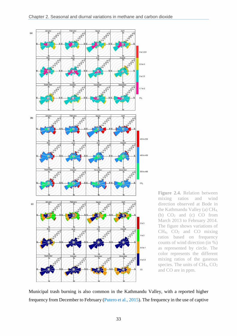
Chapter 2. Seasonal and diurnal variations in methane and carbon dioxide
33
Municipal trash burning is also common in the Kathmandu Valley, with a reported higher
frequency from December to February (Putero et al., 2015). The frequency in the use of captive
Figure 2.4. Relation between
mixing ratios and wind
direction observed at Bode in
the Kathmandu Valley (a) CH4,
(b) CO2 and (c) CO from
March 2013 to February 2014.
The figure shows variations of
CH4, CO2 and CO mixing
ratios based on frequency
counts of wind direction (in %)
as represented by circle. The
color represents the different
mixing ratios of the gaseous
species. The units of CH4, CO2
and CO are in ppm.
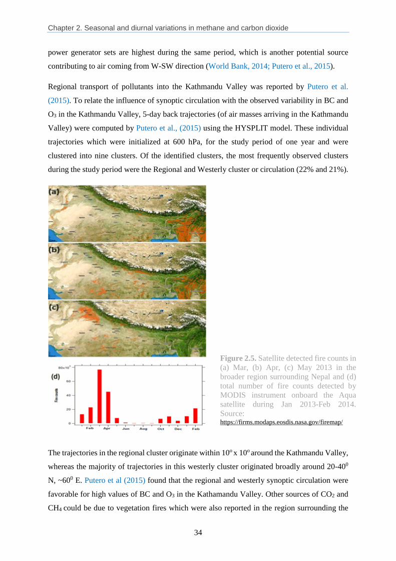
Chapter 2. Seasonal and diurnal variations in methane and carbon dioxide
34
power generator sets are highest during the same period, which is another potential source
contributing to air coming from W-SW direction (World Bank, 2014; Putero et al., 2015).
Regional transport of pollutants into the Kathmandu Valley was reported by Putero et al.
(2015). To relate the influence of synoptic circulation with the observed variability in BC and
O3 in the Kathmandu Valley, 5-day back trajectories (of air masses arriving in the Kathmandu
Valley) were computed by Putero et al., (2015) using the HYSPLIT model. These individual
trajectories which were initialized at 600 hPa, for the study period of one year and were
clustered into nine clusters. Of the identified clusters, the most frequently observed clusters
during the study period were the Regional and Westerly cluster or circulation (22% and 21%).
The trajectories in the regional cluster originate within 10o x 10o around the Kathmandu Valley,
whereas the majority of trajectories in this westerly cluster originated broadly around 20-400
N, ~600 E. Putero et al (2015) found that the regional and westerly synoptic circulation were
favorable for high values of BC and O3 in the Kathamandu Valley. Other sources of CO2 and
CH4 could be due to vegetation fires which were also reported in the region surrounding the
Figure 2.5. Satellite detected fire counts in
(a) Mar, (b) Apr, (c) May 2013 in the
broader region surrounding Nepal and (d)
total number of fire counts detected by
MODIS instrument onboard the Aqua
satellite during Jan 2013-Feb 2014.
Source: https://firms.modaps.eosdis.nasa.gov/firemap/

Chapter 2. Seasonal and diurnal variations in methane and carbon dioxide
35
Kathmandu Valley during the pre-monsoon months (Putero et al., 2015). Similarly, high
pollution events, peaking in the pre-monsoon, were observed at Nepal Climate Observatory-
Pyramid (NCO-P) near Mt. Everest, which have been associated with open fires along with the
Himalayan foothills, northern Indo-Gangetic Plain (IGP), and other regions in the Indian
Subcontinent (Putero et al., 2014). MODIS derived forest counts (Figure 2.5), which also
indicated high frequency of forest fire and farm fires from February to April and also during
post-monsoon season. It is interesting that the monthly mean CO2 mixing ratio was maximum
in April (430 ± 27 ppm) which could be linked to the fire events. It is likely that the westerly
winds (>2.5-4.5 m s-1) during the daytime (supplementary information Figure A.2, A.3) bring
additional CO2 from vegetation fires and agro-residue burning in southern plains of Nepal
including the IGP region (Figure 5). Low values of CO2 and CH4 during June-July (Figure
2.3) were coincident with the rainy season, and sources such as brick kiln emission, trash
burning, captive power generators, and regional agriculture residue burning and forest fires are
weak or absent during these months.
2.3.3. Diurnal variation
Figure 2.6 shows the average seasonal diurnal patterns of CH4, CO2, CO, and water vapor
mixing ratios observed at Bode for four seasons. All the three-gas species had distinct diurnal
patterns in all seasons, characterized by maximum values in the morning hours (peaked around
7:00-9:00), afternoon minima around 15:00-16:00, and a gradual increase through the evening
until next morning. There was no clear evening peak in CH4 and CO2 mixing ratios whereas
CO shows an evening peak around 20:00. The gradual increase of CO2 and CH4 in the evening
in contrast to the increase until evening peak traffic hours and later decay of CO may be
indicative of a few factors. As pointed out earlier, after the peak traffic hours, there are no
particularly strong sources of CO, especially in the monsoon and post-monsoon season. It is
also likely that some of the CO is decayed due to nighttime katabatic winds which replace
polluted air masses with cold and fresh air from the nearby mountain (Panday and Prinn, 2009).
As for the CO2, the biosphere respiration at night in the absence of photosynthesis can add
additional CO2 to the atmosphere which especially in the very shallow nocturnal boundary
layer may explain part of the increase of the CO2 mixing ratio. The well-defined morning and
evening peaks observed in CO mixing ratios are associated with the peaks in traffic and
residential activities. The CH4 and CO2 showed pronounced peaks in the morning hours (07:00-
09:00) in all seasons with almost the same level of seasonal average mixing ratios.

Chapter 2. Seasonal and diurnal variations in methane and carbon dioxide
36
Figure 2.6. Diurnal variations of hourly mixing ratios in different seasons (a) CH4, (b) CO2,
(c) CO, and (d) water vapor observed at Bode (semi-urban site) in the Kathmandu Valley
during March 2013-February 2014. Seasons are defined as Pre-monsoon: Mar-May, Monsoon:
Jun-Sep, Post-monsoon: Oct-Nov, Winter: Dec-Feb. The x axis is in Nepal Standard Time
(NST).
CO had a prominent morning peak in winter and pre-monsoon season, but the peak was
significantly lower in monsoon and post-monsoon. The CO (~1-1.4 ppm) around 08:00-09:00
am in winter and pre-monsoon were nearly 3-4 times higher than in monsoon and post-
monsoon season. It appears that CH4 and CO2 mixing ratios were continuously building up at
night until the following morning peak in all seasons.
The similar seasonal variations in CH4 and CO2 across all seasons could be due to their long-
lived nature, as compared to CO, whose diurnal variations are strongly controlled by the

Chapter 2. Seasonal and diurnal variations in methane and carbon dioxide
37
evolution of the boundary layer. Kumar et al. (2015) also reported morning and evening peaks
and an afternoon low in CO2 mixing ratios in industrial, commercial, and residential sites in
Chennai in India. The authors also found high early morning CO2 mixing ratios at all sites and
attributed it to the temperature inversion and stable atmospheric condition.
The daytime low CH4 and CO2 mixing ratios were due to (i) elevated mixing layer height in
the afternoon (Figure 2.7), (ii) development of upslope wind circulation in the valley, and (iii)
development of westerly and southwesterly winds which blows through the valley during the
daytime from around 11 am to 5 pm (supplementary information Figure A.2), all of which aid
in dilution and ventilation of the pollutants out of the valley (Regmi et al., 2003; Kitada and
Regmi, 2003; Panday and Prinn, 2009). In addition, the daytime CO2 minimum in the summer
monsoon is also associated with high photosynthetic activities in the valley as well as in the
broader surrounding region. In the nighttime and early morning, the mixing layer height was
low (only around 200-300 m in all seasons) and remains stable for almost 17 hours a day. In
the daytime, it grows up to 800-1200 m for a short time (ca. from 11:00 to 6:00) (Mues et al.,
2017). Therefore, the emissions from various activities in the evening after 18:00 (cooking and
heating, vehicles, trash burning, and bricks factories in the night and morning) were trapped
within the collapsing and shallow boundary layer, and hence mixing ratios were high during
evening, night and morning hours. Furthermore, plant and soil respiration also increases CO2
mixing ratio during the night (Chandra et al., 2016). However, Ganesan et al. (2013) found a
distinct diurnal cycle of CH4 mixing ratios with twin peaks in the morning (7:00-9:00), and
afternoon (15:00-17:00) and a nighttime low in winter but no significant diurnal cycle in the
summer of 2012 in Darjeeling, a hill station (2194 m asl.) in the eastern Himalaya. The authors
described that the morning peaks could be due to the radiative heating of the ground in the
morning, which breaks the inversion layer formed during night, and as a result, pollutants are
ventilated from the foothills up to the site. The late afternoon peaks match wind direction and
wind speed (upslope winds) that could bring pollution from the plains to the mountains.
The diurnal variation of CO is also presented along with CO2 and CH4 in Figure 6c. CO is an
indicator of primary air pollution. Although the CO mixing ratio showed distinct diurnal
pattern, it was different from the diurnal patterns of CO2 and CH4. CO diurnal variation showed
distinct morning and evening peaks, afternoon minima, and a nighttime accumulation or decay.
Nighttime accumulation in CO was observed only in winter and pre-monsoon and decay or
decrease in monsoon season and post-monsoon season (Figure 2.7). The lifetime of CO (weeks
to months) is very long compared to the ventilation timescales for the valley, so the different

Chapter 2. Seasonal and diurnal variations in methane and carbon dioxide
38
diurnal cycles would be due to differences in nighttime emissions. While the biosphere respires
at night which may cause a notable increase in CO2 in the shallow boundary layer, most CO
sources (transport sector, residential cooking) except brick kilns remain shut down or less
active at night. This also explains why nighttime values of CO drop less in the winter and pre-
monsoon than in other seasons. Furthermore, the prominent morning peaks of CO in pre-
monsoon and winter compared to other seasons results from nighttime accumulation, additional
fresh emissions in the morning and recirculation of the pollutants due to downslope katabatic
winds (Pandey and Prinn, 2009; Panday et al., 2009). Pandey and Prinn (2009) observed
nighttime accumulation and gradual decay during the winter (January 2005). The measurement
site in Pandey and Prinn (2009) was near the urban core of the Kathmandu Valley and had
significant influence from the vehicular sources all over the season including the winter season.
Bode lies in close proximity to the brick kilns which operate 24 hours during the winter and
pre-monsoon period. Calm southeasterly winds are observed during the nighttime and early
morning (calculated 22:00 – 8:00) in pre-monsoon and winter, which transport emissions from
brick kiln to the site (Sarkar et al., 2016). Thus, the gradual decay in CO was not observed in
Bode.
The timing of the CO morning peak observed in this study matches with observations by
Panday et al. (2009). They also found CO morning peak at 8:00 in October 2004 and at 9:00 in
January 2005. The difference could be linked to the boundary layer stability. As the sun rises
later in winter, the boundary layer stays stable for a longer time in winter keeping mixing ratios
higher in morning hours than in other seasons with an earlier sunrise. The morning peaks of
CO2 and CH4 mixing ratios occurred around 6:00-7:00 local time in the pre-monsoon,
monsoon, and post monsoon season, whereas in winter their peaks are delayed by 1-2 hours in
the morning; CH4 at 8:00 and CO2 at 9:00. The CO showed that its morning peak was delayed
compared to CO2 and CH4 morning peaks by 1-2 hour in pre-monsoon, monsoon and post-
monsoon (at 8:00) and in winter (at 9:00). The occurrence of morning peaks in CO2 and CH4
1-2 hours earlier than CO is interesting. This could be due to the long lifetimes and relatively
smaller local sources of CH4 and CO2, as CO is mainly influenced by emissions from vehicles
during rush hour, as well as from biomass and trash burning in the morning hours. Also, CO
increases irrespective of change in the mixing layer (collapsing or/rising, Figure 2.7) but CO2
and CH4 start decreasing only after the mixing layer height starts to rise. Recently, Chandra et
al. (2016) also reported that the CO2 morning peak occurred earlier than CO in observations in

Chapter 2. Seasonal and diurnal variations in methane and carbon dioxide
39
Ahmedabad City India. This was attributed to CO2 uptake by photosynthetic activities after
sunrise but CO kept increasing due to emissions from the rush hour activities.
Figure 2.7. Diurnal variations of hourly mixing ratios of CH4, CO2, CO, and mixing layer
height (MLH) at Bode (a semi-urban site in the Kathmandu Valley) in different seasons (a)
pre-monsoon (Mar-May), (b) monsoon (Jun-Sep), (c) post-monsoon (Oct-Nov) and (d) winter
(Dec-Feb) during March 2013- Feb 2014.
The highest daytime minimum of CO2 was observed in the pre-monsoon followed by winter
(Figure 2.6b). The higher daytime minimum of CO2 mixing ratios in the pre-monsoon season
than in other seasons, especially winter, is interesting. The local emission sources are similar
in pre-monsoon and winter and the boundary layer is higher (in the afternoon) during the pre-
monsoon (~1200 meters) than in winter (~900 meters) (Mues et al., 2017). Also, the biospheric
activity in the region is reported to be higher in the pre-monsoon (due to high temperature and
solar radiation) than winter (Rodda et al., 2016). Among various possible causes, transport of
CO2 rich air from outside the Kathmandu Valley has been hypothesized as a main contributing
factor, due to regional vegetation fires combined with westerly mesoscale to synoptic transport
Putero et al. (2015). In monsoon and post-monsoon seasons, the minimum CO2 mixing ratios

Chapter 2. Seasonal and diurnal variations in methane and carbon dioxide
40
in the afternoon drops down to 390 ppm, this was close to the values observed at the regional
background sites Mauna Loa and Waliguan.
2.3.4. Seasonal interrelation of CO2, CH4 and CO
The Pearson’s correlation coefficient (r) between CO2 and CO was strong in winter (0.87),
followed by monsoon (0.64), pre-monsoon (0.52) and post-monsoon (0.32). The higher
coefficient in winter indicates that common or similar sources for CO2 and CO and moderate
values in pre-monsoon and monsoon indicates the likelihood of different sources. To avoid the
influence of strong diurnal variations observed in the valley, daily averages, instead of hourly,
were used to calculate the correlation coefficients. The correlation coefficients between daily
CH4 and CO2 for four seasons are as follows: winter (0.80), post-monsoon (0.74), pre-monsoon
(0.70) and monsoon (0.22). A semi-urban measurement study in India also found a strong
positive correlation between CO2 and CH4 in the pre-monsoon (0.80), monsoon (0.61), post-
monsoon (0.72) and winter (0.8) (Sreenivas et al., 2016). It should be noted here that Sreenivas
et al., (2006) used hourly average CO2 and CH4 mixing ratios. The weak monsoon correlation
at Bode, which is in contrast to Sreenivas et al. (2016), may point to the influence of dominant
CH4 emission from paddy field during the monsoon season (Goroshi et al., 2011). Daily CH4
and CO was also weakly correlated in monsoon (0.34) and post-monsoon (0.45). Similar to
CH4 and CO2, the correlation between CH4 and CO were moderate to strong in pre-monsoon
(0.76) and winter (0.75).
Overall, the positive and high correlations between CH4 and CO mixing ratios and between
CH4 and CO2 in the pre-monsoon and winter indicate common sources, most likely combustion
related sources such as vehicular emission, brick kilns, agriculture fire etc., or the same source
regions (i.e. their transport due to regional atmospheric transport mechanisms). Weak
correlation, between CH4-CO2 and between CH4-CO, during monsoon season indicates sources
other than combustion-related may be active, such as agriculture as a key CH4 source (Goroshi
et al., 2013).
2.3.5. CO and CO2 ratio: Potential emission sources
The ratio of the ambient mixing ratios of CO and CO2 was used as an indicator to help
discriminate emission sources in the Kathmandu Valley. The ratio was calculated from the
excess (dCO and dCO2) relative to the background values of ambient CO and CO2 mixing
ratios. The excess value was estimated by subtracting the base value which was calculated as
the fifth percentile of the hourly data for a day (Chandra et al., 2016).

Chapter 2. Seasonal and diurnal variations in methane and carbon dioxide
41
Table 2.5. Emission ratio of CO/CO2 (ppb ppm-1) derived from emission factors (mass of gas
emitted from per kilogram of fuel burned, “except for the transport sector” which is derived
from gram of gases emitted per kilometer distance travelled)
Average emission ratios from the literature are shown in Table 2.5, and average ratios of
dCO/dCO2 are shown in Table 2.6, disaggregated into morning hours, evening hours, and
seasonal values. It must be stated that due to the large variance in the calculated ratio from this
study (Table 2.6) as well as the likely variation in the estimated ratio presented in Table 2.5,
the interpretation and conclusion about sources should be cautiously drawn and will be
indicative. Higher ratios were found in pre-monsoon (12.4) and winter (15.1) season compared
to post-monsoon (8.3) and monsoon (7.5). These seasonal differences in the dCO/dCO2 ratio
are depicted in Figure 8, which shows a clear relationship with the wind direction and
associated emissions, with the highest values especially for stronger westerly winds. Compared
to the other three seasons, the ratio in winter was also relatively high for air masses from the
east, likely due to emissions from brick kilns combined with accumulation during more
stagnant meteorological conditions (supplementary information Figure A.2, A.3). In other
seasons, emission emanating from the north and east of Bode were characterized by a

Chapter 2. Seasonal and diurnal variations in methane and carbon dioxide
42
dCO/dCO2 ratio below 15. Air masses from the west and south generally have a ratio from 20
to 50 in all but post-monsoon season, where the ratio sometimes exceeds 50. A ratio of 50 or
over is normally due to very inefficient combustion sources (Westerdahl et al., 2009; Stockwell
et al., 2016), such as agro-residue burning, which is common during the post-monsoon season
in the Kathmandu Valley.
For interpretability of emission ratio with sources, the ratio was classified into three categories:
(i) 0 – 15, (ii) 15 – 45, and (iii) greater than 45. This classification was based on the observed
distribution of emission ratio during the study period (Figure 2.8) and a compilation of
observed emission ratios typical for different sources from Nepal and India (see Table 2.5). An
emission ratio below 15 is likely to indicate residential cooking and diesel vehicles, and captive
power generation with diesel-powered generator sets (Smith et al., 2000; ARAI, 2008; World
Bank, 2014). The emission from brick kilns (FCBTK and Clamp kilns, both common in the
Kathmandu Valley), and inefficient, older (built before 2000) gasoline cars fall in between 15
- 45 (ARAI, 2008; Weyant et al., 2014; Stockwell et al., 2016). Four-stroke motorbikes and
biomass burning activities (mixed garbage, crop-residue and biomass) are one of the least
efficient combustion sources, with emission ratios higher than 45 (ARAI, 2008; Westerdahl et
al., 2009; Stockwell et al., 2016).
Although ratio of CO/CO2 is a weak indicator of sources and the mean ratio has large variance
(See Table 2.6), the conclusions drawn, from using Figure 2.8 and the above mentioned
classification, are not conclusive. The estimated CO/CO2 ratio tentatively indicates that the
local plume impacting the measurement site (Bode) from the north and east could be residential
and/or diesel combustion. The estimated CO/CO2 ratio of the local plume from the south and
west generally falls in the 15-45 range which could indicate emissions from brick kilns and
inefficient gasoline vehicles. Very high ratios were also estimated from the south west during
the post-monsoon season. Among other possible sources, this may indicate agro-residue open
burning.
The emission inventory for CO identifies (aggregate for a year) residential, and gasoline related
emission from transport sector (Sadavarte et al., 2019). The inventory is not yet temporally
resolved, so no conclusion can be drawn about the sources with respect to different seasons.
From the 1km x1km emission inventory of the Kathmandu Valley for 2011, the estimated
sectoral source apportionment of CO is residential (37%), transport sector (40%) and industrial

Chapter 2. Seasonal and diurnal variations in methane and carbon dioxide
43
(20%). The largest fraction from the residential sector is cooking (24 %) whereas the majority
of transport sector related CO in the Kathmandu Valley is from gasoline vehicles.
Figure 2.8. Seasonal polar plot of hourly dCO/dCO2 ratio based upon wind direction and wind
speed: (a) pre-monsoon, (b) monsoon, (c) post-monsoon and (d) winter seasons.
The dCO/dCO2 ratio also changes markedly between the morning peak hours (7:00-9:00,
except in winter season when the peak occurs during 8:00-9:00) and evening peak hours
(19:00-21:00 pm) (Table 2.6). Morning and evening values were lowest (2.2, 8.0) during the
monsoon and highest (11.2, 21.6) in the winter season, which points to the different emission
characteristics in these two seasons. This feature is similar to Ahmedabad, India, another urban
site in south Asia, where the morning/evening values were lowest (0.9/19.5) in monsoon and
highest in winter (14.3/47.2) (Chandra et al., 2016). In the morning period, the ratio generally
falls within a narrower range, from less than 1 to about 25, which indicates a few dominant
sources, such as cooking, diesel vehicles, and diesel gen-sets (see Figure 2.9). In the evening
period, the range of the ratio is much wider, from less than 1 to more than 100, especially in
winter. This is partly due to the shallower boundary layer in winter, giving local CO emissions
a chance to build up more rapidly compared to the longer-lived and well-mixed CO2, and also
indicating the prevalence of additional sources such as brick kilns and agro-residue burning.

Chapter 2. Seasonal and diurnal variations in methane and carbon dioxide
44
Table 2.6 Average (SD) of the ratio of dCO to dCO2, their Geometric mean (GeoSD) over a
period of 3 hours during (a) morning peak (b) evening peak and (c) seasonal (all hours) of the
ambient mixing ratios of CO and CO2 and their lower and upper bound (LB and UB).
Figure 2.9. Seasonal frequency distribution of hourly dCO/dCO2 ratio (a) morning hours (7:00-
9:00) in all seasons except winter (8:00-10:00), (b) evening hours (19:00-21:00).
2.3.6. Comparison of CH4 and CO2 at semi-urban site (Bode) and rural site (Chanban)
Figure 2.10 shows time series of hourly average mixing ratios of CH4, CO2, CO and water
vapor observed simultaneously at Bode and Chanban for the period of 15th July to 3rd October

Chapter 2. Seasonal and diurnal variations in methane and carbon dioxide
45
2015. The hourly meteorological parameters observed at Chanban are shown in supplementary
Figure A.4. The hourly temperature ranges from 14 to 28.5 °C during the observation period.
The site experienced calm winds during the night and moderate southeasterly winds with
hourly maximum speed of up to 7.5 m s-1 during the observation period. The CH4 mixing ratios
at Chanban varied from 1.880 ppm to 2.384 ppm, and generally increased from the last week
of July until early September, peaking around 11th September and then falling off towards the
end of the month. CO followed a generally similar pattern, with daily average values ranging
from 0.10 ppm to 0.28 ppm. The hourly CO2 mixing ratios ranged from 375 to 453 ppm, with
day to day variations, but there was no clear pattern as observed in trend like CH4 and CO
mixing ratios.
Figure 2.10. Comparison of hourly average mixing rations of CH4, CO2, CO, and water vapor
observed at Bode (a semi-urban site) in the Kathmandu Valley and at Chanban (a
rural/background site) in Makawanpur district, ~ 20 km from Kathmandu, on other side of a
tall ridge.
The CH4, CO2, and CO mixing ratios were higher in Bode than in Chanban (Figure 2.10, Table
2.4), with Chanban approximately representing the baseline of the lower envelope of the Bode
levels. The mean CO2, CH4 and CO mixing ratios over the entire sampling period of nearly
three months at Bode are 3.8%, 12.1%, and 64% higher, respectively, than at Chanban. The
difference in the CO2 mixing ratio could be due to the large uptake of CO2 in the forested area
at Chanban and surrounding regions compared to Bode, where the local anthropogenic

Chapter 2. Seasonal and diurnal variations in methane and carbon dioxide
46
emissions rate is higher and less vegetation for photosynthesis. The coincidence between the
base values of CO and CH4 mixing ratios at Bode and the levels observed at Chanban implies
that Chanban CO and CH4 mixing ratios are indicative of the regional background levels. A
similar increase in CO and CH4 mixing ratios at Chanban from July to September was also
observed at Bode, which may imply that the regional/background levels in the broader
Himalayan foothill region also influences the baseline of the daily variability of the pollutants
in the Kathmandu Valley, consistent with Panday and Prinn (2009).
Figure 2.11. Diurnal variations of hourly average mixing ratios of (a) CH4, (b) CO2, (c) CO
and (d) water vapor observed at Bode in the Kathmandu Valley and at Chanban in Makawanpur
district during 15 July- 03 October 2015.
Figure 2.11 shows the comparison of average diurnal cycles of CO2, CH4, CO and water vapor
mixing ratios observed at Bode and Chanban. The diurnal pattern of CO2 mixing ratios at both
sites is similar, but more pronounced at Bode, with a morning peak around 6:00-7:00, a daytime
minimum, and a gradual increase in the evening until the next morning peak. A prominent

Chapter 2. Seasonal and diurnal variations in methane and carbon dioxide
47
morning peak at Bode during the monsoon season indicates the influence of local emission
sources. The daytime CO2 mixing ratios are also higher at Bode than at Chanban because of
local emissions less uptake of CO2 for photosynthesis in the valley in comparison to the
forested area around Chanban. Like the diurnal pattern of CO2 depends on the evolution of the
mixing layer at Bode, as discussed earlier, it is expected that the mixing layer evolution
similarly influences the diurnal CO2 mixing ratios at Chanban. CO, on the other hand, shows
very different diurnal patterns at Bode and Chanban. Sharp morning and evening peaks of CO
are seen at Bode, indicating the strong local polluting sources, especially cooking and traffic
in the morning and evening peak hours. Chanban, in contrast, only has a subtle morning peak
and no evening peak. After the morning peak, CO sharply decreases at Bode but not at
Chanban. The growth of the boundary layer after sunrise and entrainment of air from the free
troposphere, with lower CO mixing ratios, causes CO to decrease sharply during the day at
Bode. At Chanban, on the other hand, since the mixing ratios are already more representative
of the local and regional background levels which will also be prevalent in the lower free
troposphere, CO does not decrease notably during the daytime growth of the boundary layer as
observed at Bode.
Similarly, while there is very little diurnal variation in the CH4 mixing ratios at Chanban, there
is a strong diurnal cycle of CH4 at Bode, similar to CO2 there. At Chanban, the CH4 mixing
ratio only shows a weak minimum at around 11 am, a slow increase during the day until its
peak around 22:00, followed by a slow decrease during the night and a more rapid decrease
through the morning. The cause of this diurnal pattern at Chanban is presently unclear, but the
levels could be representative of the regional background throughout the day and show only
limited influences of local emissions.
2.4 Conclusions
A cavity ring down spectrometer (Picarro G2401, USA) was used to measure ambient CO2,
CH4, CO, and water vapor mixing ratios at a semi-urban site (Bode) in the Kathmandu Valley
for a year. This was the first 12-months of continuous measurements of these four species in
the Kathmandu Valley in the foothills of the central Himalaya. Simultaneous measurement was
carried out at a rural site (Chanban) for approximately 3 months to evaluate urban-rural
differences.
The measurement also provided an opportunity to establish diurnal and seasonal variation of
these species in one of the biggest metropolitan cities in the foothills of Himalayas. Annual

Chapter 2. Seasonal and diurnal variations in methane and carbon dioxide
48
average of the mixing ratio of CH4 and CO2 in Bode revealed that they were higher than the
mixing ratios at the background sites such as the Mauna Loa, USA and Mt. Waliguan, China,
as well as higher than urban/semi-urban sites in nearby regions such as Ahmedabad and
Shadnagar in India. These comparisons highlight potential sources of CH4 and CO2 in the
Kathmandu Valley, such as brick kilns in the valley.
Polluted air masses were transported to the site mainly by two major local wind circulation
patterns, East-South and North-East and West-Southwest throughout the observation period.
Strong seasonality was observed with CO compared to CO2 and CH4. Winter and pre-monsoon
high CO are linked to emission sources active in these seasons only and are from east-southeast
and west-southwest. Emission from the east-southeast are most likely related to brick kilns
(winter and pre-monsoon), which are in close proximity to Bode. Major city-centers are located
in the west-southwest of Bode (vehicular emission) which impact the site all-round the year,
although higher during winter season. Winter high was also observed with CO2 and CH4, which
are mostly local influence of brick kilns, trash burning and emission from city-center.
Nighttime and early morning accumulation of pollutants in winter due to a shallow stable
mixing height (ca. 200 m) also contribute to elevated levels than other seasons. Diurnal
variation across all seasons indicates the influence of rush-hour emissions related to vehicles
and residential emissions. The evolution of the mixing layer height (200-1200 m) was a major
factor which controls the morning-evening peak, afternoon low and night-early morning
accumulation or decay. Thus, the geographical setting of the Kathmandu Valley and its
associated meteorology play a key role in the dispersion and ventilation of pollutants in the
Kathmandu Valley. The ratio of CO/CO2 across different seasons and wind directions
suggested that emissions from inefficient gasoline vehicles, brick kilns, residential cooking and
diesel combustion are likely to impact Bode.
The differences in mean values for urban-rural measurements at Bode and Chanban is highest
for CO (64 %) compared to CO2 (3.8%) and CH4 (12%). Low values of CH4 and CO2 mixing
ratios at the Chanban site could represent regional background mixing ratios.
This study has provided valuable information on key greenhouse gases and air pollutants in the
Kathmandu Valley and the surrounding regions. These observations can be useful as ground-
truthing for evaluation of satellite measurements, as well as climate and regional air quality
models. The overall analysis presented in the paper will contribute along with other recent

Chapter 2. Seasonal and diurnal variations in methane and carbon dioxide
49
measurement and analysis to providing a sound scientific basis for reducing emissions of
greenhouse gases and air pollutants in the Kathmandu Valley.
Chapter 2. Seasonal and diurnal variations in methane and carbon dioxide
50
Chapter 3
1. Observation and Analysis of Spatio-temporal
Characteristics of Surface Ozone and Carbon
Monoxide at Multiple Sites in the Kathmandu
Valley, Nepal
Abstract
Residents of the Kathmandu Valley experience severe particulate and gaseous air pollution
throughout most of the year, even during much of the rainy season. The knowledge base for
understanding the air pollution in the Kathmandu Valley was previously very limited, but is
improving rapidly due to several field measurement studies conducted in the last few years.
Thus far, most analyses of observations in the Kathmandu Valley have been limited to short
periods of time at single locations. This study extends the past studies by examining the spatial
and temporal characteristics of two important gaseous air pollutants (CO and O3) based on
simultaneous observations over a longer period at five locations within the valley and on its
rim, including a supersite (at Bode in the valley center, 1345 m above sea level) and four
satellite sites (at Paknajol, 1380 m asl in the Kathmandu city center, at Bhimdhunga (1522 m
asl), a mountain pass on the valley’s western rim, at Nagarkot (1901 m asl), another mountain
pass on the eastern rim, and Naikhandi (1233 m asl), near the valley’s only river outlet). CO
and O3 mixing ratios were monitored from January to July 2013, along with other gases and
aerosol particles by instruments deployed at the Bode supersite during the international air
pollution measurement campaign SusKat-ABC (Sustainable Atmosphere for the Kathmandu
Valley – endorsed by the Atmospheric Brown Clouds program of UNEP). The monitoring of
O3 at Bode, Paknajol and Nagarkot as well as the CO monitoring at Bode were extended until
March 2014 to investigate their variability over a complete annual cycle. Higher CO mixing
ratios were found at Bode than at the outskirt sites (Bhimdhunga, Naikhandi and Nagarkot),
and all sites except Nagarkot showed distinct diurnal cycles of CO mixing ratio with morning
peaks and daytime lows. Seasonally, CO was higher during pre-monsoon (March-May) season
and winter (December-February) season than during monsoon season (June-September) and
post-monsoon (October-November) season. This is primarily due to the emissions from brick
industries, which are only operational during this period (January-April), as well as increased

Chapter 2. Seasonal and diurnal variations in methane and carbon dioxide
51
domestic heating during winter, and regional forest fires and agro-residue burning during the
pre-monsoon season. It was lower during the monsoon due to rainfall, which reduces open
burning activities within the valley and in the surrounding regions, and thus reduces sources of
CO. The meteorology of the valley also played a key role in determining the CO mixing ratios.
The wind is calm and easterly in the shallow mixing layer, with a mixing layer height (MLH)
of about 250 m, during the night and early morning. The MLH slowly increases after the
sunrises and decreases in the afternoon. As a result, the westerly wind becomes active and
reduces the mixing ratio during the day time. Furthermore, there was evidence of an increase
in the O3 mixing ratios in the Kathmandu Valley as a result of emissions in the Indo-Gangetic
Plains (IGP) region, particularly from biomass burning including agro-residue burning. A top-
down estimate of the CO emission flux was made by using the CO mixing ratio and mixing
layer height measured at Bode. The estimated annual CO flux at Bode was 4.9 µg m-2 s-1, which
is 2-14 times higher than that in widely used emission inventory databases (EDGAR HTAP,
REAS and INTEX-B). This difference in CO flux between Bode and other emission databases
likely arises from large uncertainties in both the top-down and bottom-up approaches to
estimating the emission flux. The O3 mixing ratio was found to be highest during the pre-
monsoon season at all sites, while the timing of the seasonal minimum varied across the sites.
The daily maximum 8-hour average O3 exceeded the WHO recommended guideline of 50 ppb
on more days at the hilltop station of Nagarkot (159/357 days) than at the urban valley bottom
sites of Paknajol (132/354 days) and Bode (102/353 days), presumably due to the influence of
free-tropospheric air at the high-altitude site, as also indicated by Putero et al., (2015) for the
Paknajol site in the Kathmandu Valley as well as to titration of O3 by fresh NOx emissions
near the urban sites. More than 78% of the exceedance days were during the pre-monsoon
period at all sites. The high O3 mixing ratio observed during the pre-monsoon period is of a
concern for human health and ecosystems, including agroecosystems in the Kathmandu Valley
and surrounding regions.
3.1 Introduction
Air pollution is one of the major health risks globally. It was responsible for premature loss of
about 7 million lives worldwide in 2012 (WHO, 2014), with about 1.7 million of these being
in South Asian countries (India, Pakistan, Nepal and Bangladesh) in 2013 (Forouzanfar, 2015).
The latest report shows that the indoor and outdoor air pollution are each responsible for 4
million premature deaths every year (http://www.who.int/airpollution/en/). South Asia is
considered to be a major air pollution hotspot (Monks et al., 2009) and it is expected to be one

Chapter 2. Seasonal and diurnal variations in methane and carbon dioxide
52
of the most polluted regions in the world for surface ozone (O3) and other pollutants by 2030
(Dentener et al., 2006; IEA 2016; OECD 2016). Past studies have shown that the air pollution
from this region affects not only the region itself, but is also transported to other parts of the
world, including comparatively pristine regions such as the Himalayas and the Tibetan plateau
(Bonasoni et al., 2010; Ming, et al., 2010; Lüthi et al., 2015), as well as to other distant locations
such as northern Africa and the Mediterranean (Lawrence and Lelieveld, 2010).The pollutants
are also uplifted to the tropopause by convective air masses and transported to the extratropical
stratosphere during the monsoon season (Tissier and Legras., 2016; Lawrence and Lelieveld,
2010; Fueglistaler et al., 2009; Highwood and Hoskins, 1998). Air pollution is particularly
alarming in many urban areas of South Asia, including in the city of Kathmandu and the
broader Kathmandu Valley, Nepal (Chen et al., 2015; Putero et al., 2015; Kim et al., 2015;
Sarkar et al., 2016; Shakya et al., 2017). This is due to their rapid urbanization, economic
growth and the use of poor technologies in the transportation, energy and industrial sectors. In
Kathmandu topography also plays a major role: the bowl-shaped Kathmandu Valley is
surrounded by tall mountains and only a handful of passes. Topography is a key factor in
governing local circulations, where low MLH (typically in the range 250 m to 1,500 m) and
calm winds, have been observed particularly during nights and mornings. This in turn results
in poor ventilation (Mues et al., 2017). Overall, this is conducive to trapping air pollutants and
the deterioration of air quality in the valley. Effectively mitigating air pollutants in the regions
like the Kathmandu Valley requires scientific knowledge about characteristics and sources of
the pollutants. To contribute to this urgently-needed scientific knowledge base, in this study
we focus on the analysis of measurements of two important gaseous species, carbon monoxide
(CO and O3, at multiple sites in and around the Kathmandu Valley. This study analyzes data
from January 2013 to March 2014, which includes the intensive phase of an international air
pollution measurement campaign – SusKat-ABC (Sustainable Atmosphere for the Kathmandu
Valley – Atmospheric Brown Clouds) – conducted during December 2012 - June 2013
(Rupakheti et al., 2019, manuscript in preparation, submission anticipated in 1-2 months), with
measurements of O3 and CO at some sites continuing beyond the intensive campaign period
(Bhardwaj et al., 2017; Mahata et al., 2017).
CO is a useful tracer of urban air pollution as it is primarily released during incomplete
combustion processes that are common in urban areas. Forest fires and agro-residue burning in
the IGP and foothills of the Himalaya are other important contributors of CO in the region
(Bhardwaj et al., 2018; Mahata et al., 2017). CO is toxic at high concentrations indoors and
Chapter 2. Seasonal and diurnal variations in methane and carbon dioxide
53
outdoors, but our focus here is on ambient levels. The main anthropogenic sources of CO in
the Kathmandu Valley are vehicles, cooking activities (using liquefied petroleum gas,
kerosene, and firewood), and industries, including brick kilns, especially biomass co-fired kilns
with older technologies, and until recently diesel power generator sets (Panday and Prinn,
2009; Kim et al, 2015; Sarkar et al., 2016; Mahata et al., 2017; Sarkar et al., 2017).
Tropospheric O3, which is formed by photochemical reactions involving oxides of nitrogen
(NOx) and volatile organic compounds (VOCs), is a strong oxidizing agent in the troposphere.
Because of its oxidizing nature, it is also deleterious to human health and plants already at
typically polluted ambient levels (Lim et al., 2012; Burney and Ramanathan, 2014; Feng, 2015;
Monks et al., 2015). Tropospheric O3 is estimated to be responsible for about 5-20 % of
premature deaths caused by air pollution globally (Brauer et al., 2012; Lim et al., 2012; Silva
et al., 2013). It has also been estimated that high concentrations of O3 are responsible for a
global loss of crops equivalent to $ 11-18 billion annually (Avnery et al., 2011; UNEP and
WMO, 2011), a substantial fraction of which is associated with the loss in wheat in India alone
(equivalent to $ 5 billion in 2010) (Burney and Ramanathan, 2014). O3 can also serve as a good
indicator of the timing of the breakup of the nighttime stable boundary layer (when the ozone
levels increase rapidly in the morning due to downward transport from the free troposphere
(Panday and Prinn, 2009; Geiß et al., 2017).
Only a few past studies have reported measurements of ambient CO mixing ratios in the
Kathmandu Valley. Davidson et al. (1986) measured CO in the city center and found mixing
ratios between 1 and 2.5 ppm in the winter (December – February) of 1982-1983. Panday and
Prinn (2009) measured similar levels of CO mixing ratios during September 2004 – June 2005,
although the main sources of CO shifted from biofuel-dominated air pollutants from cooking
activities in the 1980s to vehicle-dominated pollutants in the 2000s. The growth rate in the
vehicle fleet has had a substantial influence on air pollution in the valley, including CO and
O3. Out of 2.33 million vehicles in Nepal, close to half of them are in the Kathmandu Valley
(DoTM, 2015). Shrestha et al. (2013) estimated annual emission of CO of 31 kt in 2010 from
a fraction of today’s vehicle fleet in the Kathmandu Valley by using data from a field survey
as input to the International Vehicle Emission (IVE) model. The model simulation considered
motorcycles, buses, taxis, vans and three wheelers, but did not include personal cars, trucks
and non-road vehicles. The studied fleets covered ~73% of the total fleet (570,145) registered
in the valley in 2010, with motorcycles being the most common vehicle (69% of the total fleet).

Chapter 2. Seasonal and diurnal variations in methane and carbon dioxide
54
Past studies have investigated the diurnal and seasonal variations of CO and O3 mixing ratios
in the Kathmandu Valley. Panday and Prinn (2009) observed distinct diurnal variations of CO
mixing ratios and particulate matter concentrations observed during September 2004 – June
2005 at Bouddha (about 4 km northwest of the SusKat-ABC supersite at Bode), with morning
and evening peaks. They found for the Kathmandu Valley that such peaks were created by the
interplay between the ventilation, as determined by the local meteorology, and the timing of
emissions, especially traffic and cooking emissions. The morning CO peak was also associated
with the recirculation of the pollutants transported down from an elevated residual pollution
layer (Panday and Prinn, 2009).
O3 was observed to have lower nighttime levels in the city center than at the nearby hilltop site
of Nagarkot (Panday and Prinn, 2009). Pudasainee et al. (2006) studied the seasonal variations
of O3 mixing ratios based on the observation for a whole year (2003-2004) in Pulchowk in the
Lalitpur district, just south of central Kathmandu Metropolitan City (KMC) in the Kathmandu
Valley. They reported seasonal O3 mixing ratios to be highest during the pre-monsoon (March
– May) and lowest in the winter (December – February). As a part of the SusKat-ABC
Campaign, Putero et al. (2015) monitored O3 mixing ratios at Paknajol, an urban site in the
center of the KMC over a full-year period (February 2013-January 2014). They also observed
similar seasonal variations in O3 mixing ratios in the valley to those observed by Pudasainee et
al. (2006), with highest O3 during the pre-monsoon (1 February – 12 May) season, followed
by the monsoon (13 May – 6 October), post-monsoon (7 October – 26 October) and winter (27
October – 31 January) seasons. They found that during the pre-monsoon season, westerly
winds and regional synoptic circulation transport O3 and its precursors from regional forest
fires located outside the Kathmandu Valley. In another study conducted as part of the SusKat-
ABC Campaign, 37 non-methane volatile organic compounds (NMVOCs) were measured at
Bode, with data recording every second, during winter of 2012-2013; the measurements
included isoprene, an important biogenic precursor of O3 (Sarkar et al., 2016). They found
concentrations to vary in two distinct periods. The first period was marked by no brick kiln
operations and was associated with high biogenic emissions of isoprene. During the second
period nearby brick kilns, which use coal mixed with biomass, were operational; they
contributed to elevated concentrations of ambient acetonitrile, benzene and isocyanic acid.
Furthermore, the authors found that oxygenated NMVOCs and isoprene combined accounted
for 72% and 68% of the total O3 production potential in the first period and second period,
respectively.

Chapter 2. Seasonal and diurnal variations in methane and carbon dioxide
55
Prior to the SusKat-ABC campaign there were no studies that simultaneously measured
ambient CO and O3 mixing ratios at multiple sites in the Kathmandu Valley over extended
periods of time. Past studies either focused on one long-term site, or on short-term observation
records at various sites (Panday and Prinn, 2009), or they investigated the seasonal
characteristics of single pollutants such as O3 at a single site in the valley (Pudasainee et al.,
2006). The most comparable past study is by Putero et al. (2015), who described O3 mixing
ratios at one SusKat-ABC site (Paknajol) in the Kathmandu city center observed during the
SusKat-ABC campaign, and discussed O3 seasonal variations. There is also a companion study
on regional CO and O3 pollution by Bhardwaj et al. (2017) which is based on O3 and CO mixing
ratios monitored at the SusKat-ABC supersite at Bode in the Kathmandu Valley for a limited
period (January-June 2013) and at two sites in India (Pantnagar in Indo-Gangetic Plain and
Nainital in Himalayan foothill). They reported simultaneous enhancement in O3 and CO levels
at these three sites in spring, highlighting contribution of regional emissions, such as biomass
burning in northwest Indo-Gangetic Plain (IGP), and regional transport to broader regional
scale pollution, including in the Kathmandu Valley. In this study, we document the diurnal and
seasonal (where applicable) characteristics and spatial distributions of CO and O3 mixing ratios
based on simultaneous observations at several locations within the valley and on the valley rim
mountains over a full year, helping to characterize the pollution within the valley and the
pollution plume entering and exiting the valley. We also compute the first top-down estimates
of CO emission fluxes for the Kathmandu Valley and compare these to CO emissions fluxes
in widely-used emission datasets such as EDGAR HTAP (Janssens-Maenhout et al., 2000),
REAS (Kurokawa et al., 2013) and INTEX-B (Zhang et al., 2009).
3.2 Study sites and methods
The Kathmandu Valley, situated in the foothills of the Central Himalaya, is home to more than
3 million people. The valley floor has an area of about 340 km2, with an average altitude of
about 1300 m above sea level (m asl.). It is surrounded by peaks of about 1900-2800 m asl.
The valley has five major mountains passes on its rim: the Nagdhunga, Bhimdhunga and
Mudku Bhanjhyang passes in the west, and the Nala and Nagarkot passes in the east, as shown
in Figure 3.1. The passes are situated at altitudes of 1480-1530 m asl. There is also one river
outlet (the Bagmati River) towards the south, which constitutes a sixth pass for air circulation
in and out of the valley (Regmi et al., 2003; Panday and Prinn, 2009). We selected five
measurement sites, including two on the valley floor (Bode and Paknajol), two on mountain
ridges (Bhimdhunga and Nagarkot) and one near the Bagmati River outlet (Naikhandi) to

Chapter 2. Seasonal and diurnal variations in methane and carbon dioxide
56
characterize the spatial and temporal variabilities of CO and O3 mixing ratios in the Kathmandu
Valley. A short description of the measurement sites is presented here and in Table 1, while
details on instruments deployed at those sites for this study are presented in Table 3.2. Further
details of the measurement sites are described in the SusKat-ABC campaign overview paper
(Rupakheti et al., 2019, manuscript in preparation).
Table 3.1 Information on the sampling sites (of the SusKat-ABC campaign) used in this study
with sampling carried out during 2013-2014 in the Kathmandu Valley. The altitude is in meter
above mean sea level (m asl.).
Bode (27.69°N and 85.40°E, 1344 m asl.): This was the supersite of the SusKat-ABC
Campaign. Bode is located in the Madhyapur Thimi municipality in the just east of the
geographic center of the valley. It is a semi-urban site surrounded by urban buildings and
residential houses scattered across agricultural lands. Within 4 km there are 10 brick kilns and
the Bhaktapur Industrial Estate towards the southeast (refer to Sarkar et al., 2016; Mahata et
al., 2017 for details). The O3 and CO instruments at Bode site were placed on the fifth floor of
a 6-story building, the tallest in the area. The inlets of the CO and O3 analyzers were mounted
on the roof top of the temporary lab, 20 m above the ground level.
Bhimdhunga: This site (27.73°N, 85.23°E, 1522 m asl.) is located on the Bhimdhunga pass on
the western rim of the valley. It is one of the lowest points on the north-south running mountain
ridge between the Kathmandu Valley to the east and a valley of a tributary of the Trishuli River
to the west. It is situated about 5.5 km from the western edge of the KMC (Kathmandu
Metropolitan City), in a rural setting with very few scattered rural houses nearby. The CO
instrument was placed on the ground floor of a small one-story building and its inlet was 2 m
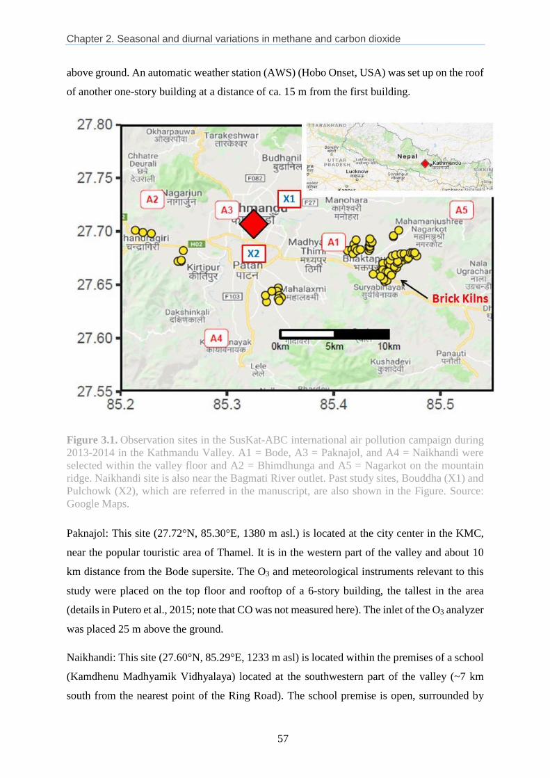
Chapter 2. Seasonal and diurnal variations in methane and carbon dioxide
57
above ground. An automatic weather station (AWS) (Hobo Onset, USA) was set up on the roof
of another one-story building at a distance of ca. 15 m from the first building.
Figure 3.1. Observation sites in the SusKat-ABC international air pollution campaign during
2013-2014 in the Kathmandu Valley. A1 = Bode, A3 = Paknajol, and A4 = Naikhandi were
selected within the valley floor and A2 = Bhimdhunga and A5 = Nagarkot on the mountain
ridge. Naikhandi site is also near the Bagmati River outlet. Past study sites, Bouddha (X1) and
Pulchowk (X2), which are referred in the manuscript, are also shown in the Figure. Source:
Google Maps.
Paknajol: This site (27.72°N, 85.30°E, 1380 m asl.) is located at the city center in the KMC,
near the popular touristic area of Thamel. It is in the western part of the valley and about 10
km distance from the Bode supersite. The O3 and meteorological instruments relevant to this
study were placed on the top floor and rooftop of a 6-story building, the tallest in the area
(details in Putero et al., 2015; note that CO was not measured here). The inlet of the O3 analyzer
was placed 25 m above the ground.
Naikhandi: This site (27.60°N, 85.29°E, 1233 m asl) is located within the premises of a school
(Kamdhenu Madhyamik Vidhyalaya) located at the southwestern part of the valley (~7 km
south from the nearest point of the Ring Road). The school premise is open, surrounded by

Chapter 2. Seasonal and diurnal variations in methane and carbon dioxide
58
sparsely scattered rural houses in agricultural lands. The nearest village (~75 houses) is about
500 m away in the southwest direction. There are 5 brick kilns within 2 km distance (2 to the
north and 3 to the northeast) from the site. The instruments were kept in a one-story building
of the school and its inlet was 5 m above the ground. The AWS (Hobo Onset, USA) was
installed on the ground near the Bagmati River, ~100 m away from the main measurement site.
Nagarkot: This site is located on a mountain ridge (27.72°N, 85.52°E, 1901 m asl), ca. 13 km
east of Bode, in the eastern part of the valley. The site faces the Kathmandu Valley to the west
and small rural town, Nagarkot, to the east. The instruments were set up in a 2-story building
of the Nagarkot Health Post and their inlets were 5 m above the ground. The AWS (Vaisala
WXT520, Finland) was set up on the roof of the building.
Table 3.2. Details of the instruments deployed at different sites during the observation period
during January 2013-March 2014 in the Kathmandu Valley.
Note: T - temperature, RH - relative humidity, SR- solar radiation, WS - wind speed, WD -
wind direction, RF- rainfall, P – pressure and MLH – Mixing layer height; ARIES - Aryabhatta
Research Institute of Observational Sciences, India; ICIMOD - International Center for
Integrated Mountain Development, Nepal; IASS – Institute for Advanced Sustainability
Studies, Germany; UVA- University of Virginia, USA; JGUM – Johannes Gutenberg
University Mainz, Germany; RTS - Real Time Solutions, Nepal; Ev-K2-CNR - Everest-
Karakorum - Italian National Research Council, Italy.
Bhimdhunga Pass in the west and Naikhandi near the Bagmati River outlet in the southwest
are the important places for interchange of valley air with outside air. The Bhimdhunga and
Naikhandi sites are approximately 5.5 and 7 km away from the nearest edge of the city,
respectively. Similarly, Bode is located downwind of the city centers and thus receives

Chapter 2. Seasonal and diurnal variations in methane and carbon dioxide
59
pollution outflow from nearby city centers of Kathmandu and Lalitpur due to strong westerly
and southwesterly winds (4-6 m s-1) during the day time, and emissions from the Bhaktapur
area to the east and southeast direction by calm easterly winds (< 1 m s-1) during the night
(Sarkar et al., 2016; Mahata et al., 2017).
A freshly calibrated new CO analyzer (Horiba APMA-370, Japan) was deployed for the first
time at Bode. This instrument is based on the IR absorption method at 4.6 µm by CO molecules.
Before field deployment at Bode, it was compared with the bench model of the Horiba (APMA-
370), and the correlation (r) between them was 0.9 and slope was 1.09. The instrument was
regularly maintained by running auto-zero checks (Bhardwaj et al., 2017). Similarly, another
CO analyzer (Picarro G2401, USA) which is based on cavity ring-down spectroscopy
technique (CRDS) was also a new factory calibrated unit, and was deployed in Bode along
with the Horiba APMA-370. An IR-based Horiba CO monitor (APMA-370) was run
simultaneously with a co-located cavity ring down spectrometry based Picarro CO analyzer for
nearly 3 months. The correlation coefficient and slope between the two measurements were
found to be 0.99 and 0.96, respectively (Mahata et al., 2017). This indicates that there was very
little drift in the IR-based CO values due to room temperature change, within acceptable range
(i.e., within the measurement uncertainties of the instruments). Therefore, we did not any apply
correction in the IR-based CO data. All other CO analyzers (Thermo Scientific, 48i-TLE,
USA), which are also based on IR absorption by CO molecules, deployed at Bhimdhunga,
Naikhandi and Nagarkot, were set up for regular automatic zero checks on a daily basis. In
addition, a span check was also performed during the observations by using span gas of 1.99
ppm (Gts-Welco, PA, USA) on March 8, 2013 at Naikhandi and Nagarkot, and on March 9 at
Bhimdhunga. The IR-based CO instruments’ span drifts were within a 5 % range.
For the O3 monitor (Teledyne 400E, USA) at Bode, regular zero and span checks were carried
out using the built-in O3 generator and scrubber (Bhardwaj et al., 2017). This unit was used in
Bode from 01 January 2013 to 09 June 2013. New factory-calibrated O3 monitors (Thermo
Scientific, 49i, USA) were used for the rest of the measurement period (18 June 2013 to 31
December 2013) at Bode, and for the full year of measurements at Nagarkot. A Thermo
Environmental O3 analyzer (Model 49i, USA) was used at the Paknajol site (Putero et al., 2015)
with the same experimental set up as described in Cristofanelli et al. (2010). The working
principle of all of the O3 instruments is based on the attenuation of UV radiation by O3
molecules at ~254 nm.

Chapter 2. Seasonal and diurnal variations in methane and carbon dioxide
60
In order to characterize observations across the seasons, we considered the following seasons
as defined in Shrestha et al. (1999) and used in other previous studies in the Kathmandu Valley
(Sharma et al., 2012; Chen et al., 2016; Mahata et al, 2017): Pre-monsoon (March, April, May);
Monsoon (June, July, August September); Post-monsoon (October, November); and Winter
(December, January, February).
3.3 Results and discussion
3.3.1 CO mixing ratio at multiple sites
Figure 3.2. Hourly average CO mixing ratios observed at supersite (Bode) and three satellite
sites (Bhimdhunga, Naikhandi and Nagarkot) of the SusKat-ABC international air pollution
measurement campaign during January to July 2013 in the Kathmandu Valley. The dotted box
represents a period (13 February - 03 April, 2013) during which data for all four sites were
available.
Figure 3.2 shows the time series of the hourly average CO mixing ratios at the four sites (Bode,
Bhimdhunga, Naikhandi and Nagarkot). Fluctuations in CO mixing ratios were higher during

Chapter 2. Seasonal and diurnal variations in methane and carbon dioxide
61
the winter and pre-monsoon than during the monsoon season at all sites. The monsoon rain
generally starts in Nepal around mid-June. In 2013, however, there were more frequent rain
events in the month of May than in previous years.
The CO mixing ratios (measured in parts per billion by volume, hereafter the unit is denoted
as ppb) of hourly averaged data over the total observation periods at four sites and their
standard deviation were: Bode - 569.9 ± 383.5 ppb during 1 January - 15 July, Bhimdhunga -
321.5 ± 166.2 ppb during 14 Jan - 15 July, Naikhandi - 345.4 ± 147.9 ppb during 3 January -
6 June and Nagarkot - 235.5 ± 106.2 ppb during 13 February - 15 July (except 4 April to 7
June). Nagarkot had only about 3 months of CO data (due to a problem in zeroing of the
instrument) during the observation period. For the measurement period, the CO mixing ratio at
Nagarkot (~13 km far from Bode) showed small fluctuations compared with the other sites.
High CO values in the Kathmandu Valley during the dry season (November-May) were also
reported by Panday and Prinn (2009) based on their measurements during September 2004-
May 2005 at Bouddha (~ 4 km in northwest from Bode). The simultaneous episodes of high
CO observed from April 1to15 in Bhimdhunga, Bode and Naikhandi indicate the influence of
regional sources, in addition to local sources. This is discussed further in section 3.2.3.
3.3.2 Diurnal and seasonal variations of CO
3.3.2.1 Diurnal pattern of CO at multiple sites
Figure 3.3 shows the diurnal cycles of CO mixing ratios at four sites (plotted for the period of
13 February to 3 April 2013, when the data were available from all four sites). The variation
in the mixing ratios during the day was characterized by a pronounced morning peak, a weaker
evening peak, and a daytime low; except at Nagarkot where peaks are less visible. Multiple
sources contribute to the morning and evening peaks, especially emission from vehicles,
residential burning (fossil fuel and biomass), brick kilns and trash burning (Kim et al., 2015;
Sarkar et al., 2016; Mahata et al., 2017). Other studies conducted during the SusKat-ABC
campaign have identified garbage (household waste and yard waste) burning as a key source
of various air pollutants, such as organic carbon (OC) and elemental carbon (EC) (Kim et al.,
2015), poly-cyclic aromatic hydrocarbon (PAHs) (Chen et al., 2015), and NMVOCs (Sarkar et
al., 2016; Sarkar et al., 2017). Garbage burning is often done in small fires and quite sporadic,
normally taking place in the evenings and mornings (partly chosen to avoid attention from the
responsible authorities). The rate of waste (and also biomass) burning in the morning is higher
in winter due to the use of the fires for providing warmth on colder days.

Chapter 2. Seasonal and diurnal variations in methane and carbon dioxide
62
Figure 3.3. Diurnal variations of hourly average CO mixing ratios during the common
observation period (13 February–03 April, 2013) at Bode, Bhimdhunga, Naikhandi and
Nagarkot. The lower end and upper end of the whisker represents 10th and 90th percentile,
respectively; the lower end and upper end of each box represents the 25th and 75th percentile,
respectively, and the black horizontal line in the middle of each box is the median for each
month. Note: the y-axis scale of Bode is twice that of the other three sites.
The observed diurnal cycle of CO is similar to that reported in a previous study (Panday and
Prinn, 2009), and is also similar to the diurnal pattern of black carbon (BC) in the Kathmandu
Valley (Sharma et al., 2012; Mues et al., 2017). The diurnal cycles of these primary pollutants
are closely coupled with the valley’s boundary layer height, which is about 1200 m during
daytime, and falls to approximately 200 m at nighttime in Bode (Mues et al., 2017). Nagarkot
and Bhimdhunga, both on mountain ridges, are generally above the valley’s boundary layer,
especially at night, and thus the diurnal profile especially at Nagarkot is distinct compared to
other three sites, being relatively flat with small dip during 12:00-18:00 LT (local time).

Chapter 2. Seasonal and diurnal variations in methane and carbon dioxide
63
Distinct morning peaks were observed in Bode, Bhimdhunga and Naikhandi at 08:00, 09:00,
and 10:00, respectively, i.e., the morning peak lags by 1-2 hours in Bhimdhunga and Naikhandi
compared to Bode. Bhimdhunga on the mountain ridge may receive the Kathmandu Valley’s
pollution due to upslope winds (~2 m s-1) from the east direction in the morning hours after the
dissolution of the valley’s boundary layer due to radiative heating of the mountain slopes.
However, Naikhandi is in close proximity to brick kilns and could be impacted by their plumes
carried to the site by northerly winds in the early morning (ca. 07:00-10:00, not shown). The
evening peak values at Bode and Bhimdhunga were less pronounced compared to the morning
maxima. The morning peak at Bode was influenced by nighttime accumulation of CO along
with other pollutants from nearby brick kilns (Sarkar et al., 2016; Mahata et al., 2017; Mues et
al., 2017) and recirculation of air from above (Panday and Prinn, 2009). Similarly, the local
pollution from the nearby village and city area due to upslope winds from the valley floor is
expected to contribute to the morning peak at Bhimdhunga. The evening peak at Naikhandi
was at 21:00 and was closer to the morning values in comparison to the large difference
between morning and evening peaks at Bode and Bhimdhunga. A nighttime build-up (linear
increase) of various pollutants compared to the afternoon minimum was typically observed in
Bode during the SusKat-ABC measurement period, including the main campaign period
(Sarkar et al., 2016; Mahata et al., 2017; Mues et al., 2017). This is mainly associated with the
persistent emissions such as those from brick kilns, which are in close proximity to the Bode
measurement site under the stable boundary layer. The isolated peak during the morning
transition phase at Bhimdhunga could be due to an elevated polluted layer because of the slope
wind (Panday et al., 2009). There appears to be less influence of nighttime polluting sources at
Naikhandi and Bhimdhunga than at Bode.
The MLH starts increasing after radiative heating of the surface by incoming solar radiation.
The heating of the ground causes thermals to rise from the surface layer resulting in the
entrainment of cleaner air from above the boundary layer leading to the dissolution of nocturnal
stable boundary layer. Increasing wind speeds (4-6 m s-1) during daytime also support turbulent
vertical diffusion, as well as flushing of the pollution by less polluted air masses from outside
the valley, with stronger horizontal winds allowing significant transport of air masses into the
valley. In addition, reduced traffic and household cooking activities during daytime compared
to morning and evening rush hours contribute to the reduced CO mixing ratios.

Chapter 2. Seasonal and diurnal variations in methane and carbon dioxide
64
3.3.2.2 CO diurnal variation across seasons
Due to the lack of availability of simultaneous CO data at all sites covering the entire sampling
period, a one-month period was selected for each season to examine the diurnal variation across
the seasons, and to get more insights into the mixing ratios at different times of the day, as
reported in Table 3.4. Figure 3.4 shows the diurnal variation of CO mixing ratios in Bode,
Bhimdhunga, and Naikhandi during the selected periods for the three seasons.
The diurnal cycles during each season had different characteristics. The most prominent
distinction was that the CO mixing ratio was low during the monsoon period over all sites
(Figure 3.4, Table 3.4) as a result of summer monsoon rainfall in the valley, which is 60 - 90%
Figure 3.4. Comparison of diurnal
variation of hourly average CO mixing
ratios for four seasons at Bode,
Bhimdhunga and Naikhandi. Due to the
lack of continuous data at some sites,
data of one month in each season were
taken for comparison as representative
of the winter (16 Jan – 15 Feb), pre-
monsoon (16 Mar – 15 Apr) and
monsoon (16 Jun – 15 Jul) season of
2013. Note: y-axis scale of the top panel
(Bode) is double than lower two panels
(Bhimdhunga and Naikhandi).

Chapter 2. Seasonal and diurnal variations in methane and carbon dioxide
65
of the 1400 mm rainfall for a typical year (Nayava, 1980; Giri et al., 2006). Because of the
rainfall, the brick production activities are stopped in the valley (usually they are operational
from January-April every year). Further, the rainfall also diminishes many burning activities
(forest fires, agro-residue and trash burning) within the valley and surrounding region, and thus
reduces CO emissions. Afternoon CO mixing ratios were higher in the pre-monsoon season
than in the other two seasons in Bode, Bhimdhunga and Naikhandi (also see Table 3.4), with
the most likely sources being emissions from forest fires and agro-residue burning arriving
from outside the valley during this season (this will be discussed further in section 3.2.3).
Nighttime accumulation was observed in Bode and Bhimdhunga, but not at Naikhandi, where
the mixing ratio decreased slightly from about 20:00 until about 04:00, after which the mixing
ratios increased until the morning peak. The nighttime accumulation of CO in Bode during pre-
monsoon and winter is due to the influence of nearby brick kilns (Mahata et al., 2017) because
of the calm easterly wind (refer supplementary Figure A.2 in Mahata et al., 2017). Previous
studies carried out at the Bode site during the SusKat-ABC campaign have attributed over a
dozen brick kilns located near Bode as strong sources of BC and EC (Kim et al., 2015; Mues
et al., 2017), NMVOCs (Sarkar et al, 2016; Sarkar et al., 2017), SO2 (Kiros et al., 2016) and
CO (Mahata et al., 2017), and the enhanced concentrations were observed during nighttime
and mornings when winds blew from east and southeast bringing emissions from the location
of the brick kilns to the observation site.
Bhimdhunga is not near any major polluting sources such as brick kilns, and it is unclear
whether the nighttime CO accumulation in Bhimdhunga is primarily due to ongoing local
residential pollution emissions, and/or to pollution transported from remote sources. The
transition of the wind from westerlies during the day to easterlies during the night, with
moderate wind speed (~2-4 m s-1) at Bhimdhunga, may bring polluted air masses westwards
which were initially transported to the eastern part from the Kathmandu Valley during the
daytime (Regmi et al., 2003; Panday and Prinn, 2009; Panday et al., 2009).
The distinct shift in the morning peak was seen at all 3 sites by season. The one hour shift in
the morning peak from the pre-monsoon to winter is due to an earlier onset of the morning
transition. However, the one hour difference in the morning peak between Bode (pre-monsoon
at 8:00; winter at 9:00) and Bhimdhunga/Naikhandi (pre-monsoon at 9:00 LT; winter at 10:00
LT) in the pre-monsoon and winter is associated with commencement of early local emissions

Chapter 2. Seasonal and diurnal variations in methane and carbon dioxide
66
under the shallow boundary layer at Bode. The one hour lag in the morning peak at
Bhimdhunga and Naikhandi may be due to transport of city pollutants to the site, respectively.
Across the seasons, the afternoon (12:00-16:00 LT) CO mixing ratio was higher during the
pre-monsoon than in the winter at all three stations (p value for all sites < 0.5) (Table 3.4),
although the mixing layer was higher in the pre–monsoon season than in the winter in Bode
(and presumably at the other sites as well). This is not likely to be explained by local emissions
in the valley, since these are similar in the winter and pre-monsoon periods. Putero et al. (2015)
suggested instead that this reflects an influx of polluted air into the valley due to large synoptic
circulation patterns during the pre-monsoon season. Such regional influences are explored
further in the next section.
3.3.2.3 Regional influence on CO in the valley
Recent studies have indicated the likelihood of regional long-range transport contributing to
air pollution in different parts of Nepal (Marinoni et al., 2013; Tripathee et al., 2014; Dhungel
et al., 2016; Rupakheti et al., 2016; Lüthi et al., 2016; Wan et al., 2017), including the
Kathmandu Valley, especially during the pre-monsoon period (Panday and Prinn, 2009; Putero
et al., 2015; Bhardwaj et al., 2017). During the pre-monsoon season, frequent agro-residue
burning and forest fires are reported in the IGP region including southern Nepal and the
Himalayan foothills in India and Nepal (Ram and Sarin, 2010; Vadrevu et al., 2012), and in
the Kathmandu Valley. This season is also characterized by the strongest daytime local wind
speeds (averaging 4-6 m s-1) in the Kathmandu Valley (Mahata et al., 2017). Our study also
observed several episodes of days with both elevated CO mixing ratios (Figure 3.2) and O3
mixing ratios (also measured in parts per billion by volume, hereafter the unit is denoted as
ppb) (Figure 3.5) during April and May, especially during the late afternoon period. The
influence of regional pollutants was investigated by comparing a 2-week period with normal
CO levels (16–30 March (hereafter “period I”) with an adjacent two week period (1-15 April)
with episodically high CO mixing ratios (hereafter “period II”), which nicely fit with the
“burst” in regional fire activity presented by Putero et al. (2015) in their Figure 3.9. The t-test
of the two-hourly data means of CO in period I and period II at Bode, Bhimdhunga and
Naikhandi (as in Figure 3.5) were performed at 95% confidence level and the differences were
found to be statistically significant (p < 0.5).
Figure 3.5a shows the diurnal cycle of CO mixing ratios during period I (faint color) and period
II (dark color) at Bode, Bhimdhunga and Naikhandi.

Chapter 2. Seasonal and diurnal variations in methane and carbon dioxide
67
Figure 3.5. Comparison of hourly average CO mixing ratios during normal days (March 16-
30), labelled as period I (faint color) and episode days (April 1-15), labelled as period II (dark
color) in 2013 at (a) Bode, Bhimdhunga and Naikhandi in the Kathmandu Valley. The wind
roses at Bode corresponding to two periods are also plotted (b) period I and (c) period II
respectively.
The difference between two periods was calculated by subtracting the average of period I from
average of period II. The average CO mixing ratios during period II were elevated with respect
to period I by 157 ppb at Bode, 175 ppb at Bhimdhunga, and 176 ppb at Naikhandi.

Chapter 2. Seasonal and diurnal variations in methane and carbon dioxide
68
The enhancements in mixing ratios at the three sites were fairly similar from hour to hour
throughout the day, with the exception of the late afternoon when the enhancement was
generally greatest. This consistency across the sites suggests that the episode was caused by a
large-scale enhancement (regional contribution) being added onto the prevailing local pollution
levels at all the sites. A large-scale source would also be consistent with the greater
enhancements of CO at the outskirt sites, which would be most directly affected by regional
pollution, compared to the central valley site of Bode, with strong local sources. The
enhancement during the period II is substantial (statistically significant as mentioned above),
representing an increase of approximately 45% at the outskirt sites of Bhimdhunga and
Naikhandi (which start with lower CO levels), and 23% at Bode. During both periods I and II,
local winds from west (the opposite direction from the brick kilns, which were mostly located
to the southeast of Bode) were dominant during daytime at Bode (Figure 3.5b, c). This suggests
that the elevation in CO levels was caused by additional emissions in period II in the regions
to the west and southwest of the Kathmandu Valley, e.g., large scale agricultural burning and
forest fires during this period, as also noted by Putero et al. (2015) (see their Figure 3.9). Far
away, in Lumbini in the southern part of Nepal (Rupakheti et al., 2016), and Pantnagar in
northern IGP in India (Bharwdwaj et al., 2017), about 220 km (aerial distance) to the southwest
and 585 km to the west, respectively, of the Kathmandu Valley, CO episodes were also
observed during the spring season of 2013, providing a strong indication that the episode in
period II was indeed regional in nature.
3.3.3 O3 in the Kathmandu Valley and surrounding areas
Figure 3.6 shows the hourly average and daily maximum 8-hour average of O3 mixing ratios
at Bode, Paknajol, and Nagarkot from measurements during the SusKat campaign and
afterwards, along with O3 mixing ratios from a previous study (November 2003 - October 2004;
Pudasainee et al., 2006) at the Pulchowk site (4 km away from Paknajol) in the Latitpur district.
The daily maximum 8-hour average O3 was calculated by selecting the maximum O3 mixing
ratio from 8 hour running averages during each day. The nighttime mixing ratio of hourly O3
drops close to zero in Bode, Paknajol and Pulchowk in the winter season. This is a typical
characteristic of many urban areas where reaction with NO at night depletes O3 from the
boundary layer (e.g., Talbot et al., 2005). In the pre-monsoon and monsoon months, the
titration is not as strong and the hourly O3 falls, but generally remains above 10 ppb. Similar
patterns of ozone mixing ratios were observed at other sites in northern South Asia.

Chapter 2. Seasonal and diurnal variations in methane and carbon dioxide
69
Figure 3. 6. Time series of hourly average (faint colored line) and daily maximum 8-hr average
(solid colored circle) O3 mixing ratio at (a) Bode (semi-urban), (b) Paknajol (urban) and (c)
Nagarkot (hilltop) observed during 2013-2014, and (d) Pulchowk (urban) observed during
November 2003-October 2004 in the Kathmandu Valley. Black dotted line represents WHO
guideline (50 ppb) for daily maximum 8-hr average of O3.
For example, higher O3 mixing ratios were observed in the afternoon (84 ppb) and lower during
the night and early morning hours (10 ppb) at Kullu Valley, a semi-urban site located at 1154
m asl, in the North-western Himalaya in India (Sharma et al. 2012). A similar dip in O3 value
in the dark hours was observed at Ahmedabad, India by Lal et al. (2000). Nagarkot, in contrast,
is above the valley’s boundary layer and has lesser NO for titration at night at this hill station
as has been observed in another hill station in Himalayan foothills (Naja and Lal, 2002). Thus,
the O3 level remains above 25 ppb during the entire year at Nagarkot. As also shown in Table
3.3, at all sites, the O3 mixing ratios were highest in the pre-monsoon, but the timing of the
lowest seasonal values varied across the sites: post-monsoon in Bode, winter in Paknajol and
monsoon in Nagarkot. Such differences in minimum O3 across the sites can be anticipated due
to the locations of the sites (e.g., urban, semi-urban, rural and hilltop sites, with differing
availabilities of O3 precursors from different emission sources). The seasonal variations of O3
observed at Bode in this study are consistent with Putero et al. (2015) and Pudasainee et al.
(2006), who also observed O3 maxima during the pre-monsoon, but O3 minima during the
winter season.
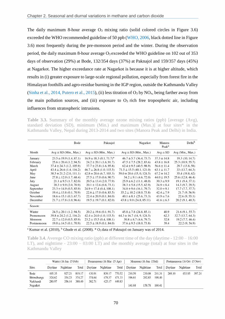
Chapter 2. Seasonal and diurnal variations in methane and carbon dioxide
70
The daily maximum 8-hour average O3 mixing ratio (solid colored circles in Figure 3.6)
exceeded the WHO recommended guideline of 50 ppb (WHO, 2006, black dotted line in Figure
3.6) most frequently during the pre-monsoon period and the winter. During the observation
period, the daily maximum 8-hour average O3 exceeded the WHO guideline on 102 out of 353
days of observation (29%) at Bode, 132/354 days (37%) at Paknajol and 159/357 days (45%)
at Nagarkot. The higher exceedance rate at Nagarkot is because it is at higher altitude, which
results in (i) greater exposure to large-scale regional pollution, especially from forest fire in the
Himalayan foothills and agro-residue burning in the IGP region, outside the Kathmandu Valley
(Sinha et al., 2014, Putero et al., 2015), (ii) less titration of O3 by NOx, being farther away from
the main pollution sources, and (iii) exposure to O3 rich free tropospheric air, including
influences from stratospheric intrusions.
Table 3.3. Summary of the monthly average ozone mixing ratios (ppb) [average (Avg),
standard deviation (SD), minimum (Min.) and maximum (Max.)] at four sites* in the
Kathmandu Valley, Nepal during 2013-2014 and two sites (Manora Peak and Delhi) in India.
a Kumar et al. (2010), b Ghude et al. (2008). * O3 data of Paknajol on January was of 2014.
Table 3.4. Averege CO mixing ratio (ppb) at different time of the day (daytime - 12:00 – 16:00
LT), and nighttime - 23:00 – 03:00 LT) and the monthly average (total) at four sites in the
Kathmandu Valley

Chapter 2. Seasonal and diurnal variations in methane and carbon dioxide
71
The diurnal profiles of O3 mixing ratios (Figure 3.7) at three sites Bode and Pakanajol in the
Valley and Nagarkot, a hilltop site normally above the Kathmandu Valley’s boundary layer
show, notably in the morning hours, that the residual layer above the Kathmandu Valley’s
mixing layer contains a significant amount of ozone. Based on the surface ozone data collected
at Paknajol during 2013-14, Putero e al. (2015) concluded that downward mixing of ozone
from the residual layer contributes to surface ozone in the Kathmandu Valley in the afternoon
hours (11:00-17:00 LT). It is likely that the same source has also contributed to higher ozone
mixing ratios at Nagarkot. Such mixing has been observed at other sites as well. Wang et al.
(2012) reported the increase in downward mixing of O3 from the stratosphere to the middle
troposphere (56%) and the lower troposphere (13%) in spring and summer in Beijing. The
downward flux was highest in the middle troposphere (75%) in winter. Similarly, Kumar et al.
(2010) reported that more than 10 ppb of stratospheric contribution at a high-altitude site (in
Nainital) during January to April. However, there were no significant stratospheric intrusions
seen in spring and summer (seen only in winter) at Nepal Climate Observatory-Pyramid
(Putero et al., 2016).
During the SusKat-ABC campaign in 2013 and later in 2014, passive sampling of gaseous
pollutants (SO2, NOx, NH3 and O3) was carried out at fourteen sites including urban/semi-urban
sites (Bode, Indrachowk, Maharajganj, Mangal Bazar, Suryabinayak, Bhaisepati,
Budhanilkantha, Kirtipur, and Lubhu) and rural sites (Bhimdhunga, Naikhandi, Sankhu,
Tinpiple, and Nagarkot) in the Kathmandu Valley (Kiros et al., 2016). Similar to this study,
they also observed higher O3 mixing ratios in rural areas than the urban/semi-urban sites in the
Kathmandu Valley. Exceedances of the WHO standard is most common during the pre-
monsoon season, occurring 78% (72/92 days), 88% (78/89 days) and 92% (85/92 days) of the
time at Bode, Paknajol and Nagarkot, respectively. A study by Putero et al., (2015), based on
O3 mixing ratio measurements at Paknajol in the Kathmandu Valley, as a part of the SusKat-
ABC campaign, has reported that the dynamics (both by horizontal and vertical winds) plays a
key role in increased O3 mixing ratios in the afternoon in the Kathmandu Valley. They
estimated that the contribution of photochemistry varied as a function of the hour of the day,
ranging from 6 to 34 %. Unfortunately, no viable NOx measurements were obtained at any site
in the Kathmandu Valley and surrounding mountain ridges during the SusKat-ABC campaign.
Speciated VOCs were measured at Bode only for about 2 months but NOx was not available
for the same period. Therefore, we were not able to discern quantitatively proportional
contributions of NOx, VOCs and intrusion (chemistry vs. dynamics) from the free troposphere
Chapter 2. Seasonal and diurnal variations in methane and carbon dioxide
72
or lower stratosphere to observed O3 concentrations at Nagarkot, Bode and other sites in the
valley. In the context of protecting public health, crops and regional vegetation, the O3 mixing
ratios in the Kathmandu Valley and surrounding areas clearly indicate the urgent need for
mitigation action aimed at reducing emissions of its precursor gases NOx and VOCs. However,
air quality management plans need to consider carefully the reduction strategies of NMVOCs
or NOx while aiming at mitigating the O3 pollution in the Kathmandu Valley. If the correct
strategy (NMVOCs vs. NOx) is not applied, then O3 mixing ratios could increase, for example,
as seen in Huszar et al. (2016) where they reported that reducing NMVOCs in urban areas in
central Europe leads to O3 reduction whereas the focus on NOx reduction results in O3 increase.
The SusKat-ABC O3 data can be compared to observations made about a decade ago by
Pudasainee et al. (2006) at the urban site of Pulchowk, not far from Paknajol, as plotted in
Figure 6d. The daily maximum 8-hour average O3 had exceeded the WHO guideline at
Pulchowk for 33% (95/292 days) of days during the observation from November 2003 to
October 2004. The exceedance was 38% (133/354 days) of days at Paknajol during Feb 2013
- March 2014. Due to inter-annual variability and differences in the seasonal observation time
periods at Pulchowk and Pakanajol, we cannot draw any conclusions about trends over the
decade between the observations because of the difference in location and sampling height as
well as a general difference in instrument calibration. However, a clear similarity between the
observations is that most of the exceedance took place during pre-monsoon season, during
which both studies have observations throughout the season (~90 days). The percentage of
exceedance at Pulchowk during the pre-monsoon season in 2003-2004 was 70% (63/90 days)
and at Pakanajol in 2013 it was 88% (78/89 days). However, just like for the annual fraction
of exceedances, due to inter-annual variability we cannot say that the 18% (or ca. 15 days)
difference in the exceedances is significant. A longer term O3 record would be needed to really
establish if there is a trend in the ozone concentrations.
3.3.4 O3 seasonal and diurnal variation
The seasonal average O3 mixing ratios at Bode, Nagarkot and Paknajol are shown in Table 3.3.
For comparison, the O3 mixing ratios measured at two sites in India, (i) Manora Peak (1958 m
asl), ca. 9 km from Nainital city, a site in rural mountain setting and (ii) Delhi, a highly-polluted
urban setting in northwest IGP are also listed in the Table, based on results from Kumar et al.
(2010) and Ghude et al. (2008). There is a strong similarity between the urban and semi-urban

Chapter 2. Seasonal and diurnal variations in methane and carbon dioxide
73
sites in Nepal (i.e., Bode, Pakanajol) and India (i.e., Delhi), as well as between the rural and
mountain sites in Nepal (i.e., Nagarkot) and India (i.e., Manora Peak), with small differences.
The peak mixing ratios were in the pre-monsoon period: at the rural and mountain sites the
peak ozone mixing ratio values were very similar (64 and 62 ppb for Nagarkot and Manora
Peak, respectively) and are due to influences discussed earlier for Nagarkot; at the sub-urban
and urban sites the pre-monsoon values are significantly lower (ca. 40, 42, 33 ppb for Bode,
Paknajol, Delhi, respectively) due to fresh NOx emissions near the urban sites and the
consequent titration of ozone with NO. The lowest O3 seasonal values at rural and mountain
sites typically occur in the monsoon months while for semi-urban and urban sites, the minimum
was observed during post-monsoon (Bode) and winter (Paknajol).
Figure 3.7. Diurnal pattern of hourly average O3 mixing ratio for different seasons during
January 2013-January 2014 at (a) Bode, (b) Paknajol, and (c) Nagarkot in the Kathmandu
Valley. The four seasons (described in the text) are defined as: pre-monsoon (Mar-May),
monsoon (Jun-Sep), post-monsoon (Oct-Nov), winter (Dec-Feb).

Chapter 2. Seasonal and diurnal variations in methane and carbon dioxide
74
Figure 3.7 shows the diurnal variation of O3 mixing ratios at Bode, Paknajol and Nagarkot in
the different seasons. The typical O3 maximum mixing ratio in the early afternoon at the urban
and semi-urban sites is mainly due to daytime photochemical production as well as entrainment
of ozone due to dynamics (both intrusion of ozone rich free tropospheric air into the boundary
layer, and regional scale horizontal transport of ozone), as explained in case of Paknajol by
Putero et al. (2015).
The ozone mixing ratios are relatively constant throughout the day at Nagarkot (~1901 m asl),
which, being a hilltop site, is largely representative of the lower free tropospheric regional
pollution values, however, it is also affected by ozone production from precursors transported
from the Kathmandu Valley due to westerly winds during the afternoon hours. The dip in O3
at Nagarkot (Figure 3.7) in the morning transition hours indicates the upward mixing of air
from polluted (and Ozone-depleted) nocturnal boundary layer as it is breaking up.
3.3.5 CO emission flux estimate
It is possible to determine a top-down estimate of the average CO emission flux for the morning
hours for the region around the Bode site by applying an approach that was developed and used
in Mues et al. (2017) to estimate the emission fluxes of BC at Bode. The analysis of Mues et
al. (2017) found BC fluxes for the Kathmandu Valley that were considerably higher than the
widely-used EDGAR HTAP emission database (Version 2.2). Support for this top-down
estimate was found by considering the BC concentrations and fluxes for the Kathmandu Valley
in comparison to Delhi and Mumbai; although the observed BC concentrations were similar in
all three locations, the EDGAR HTAP V2.2 emissions of BC for the Kathmandu Valley are
much lower than those for Delhi and Mumbai, while the top-down emissions estimate for the
Kathmandu Valley were similar to the emissions from EDGAR HTAP V2.2 for Delhi and
Mumbai (Mues et al., 2017).
Here we apply the same method as developed in Mues et al. (2017) to estimate the CO fluxes
based on the observed CO mixing ratio and ceilometer observations of the mixing layer height
(MLH) in Bode for the period of 1 year (March 2013-February 2014). Using the approach used
by Mues et al. (2017), the CO fluxes can be calculated from the increase in CO concentrations
during the nighttime period when the MLH is nearly constant, using:

Chapter 2. Seasonal and diurnal variations in methane and carbon dioxide
75
𝐹𝐶𝑂(𝑡𝑥, 𝑡𝑦) = ∆CO × 𝑎𝑣𝑒(𝑀𝐿𝐻(𝑡𝑥), 𝑀𝐿𝐻 (𝑡𝑦))
∆𝑡 × 3600 ×
𝑀𝐿𝐻(𝑡𝑦)
𝑀𝐿𝐻 (𝑡𝑥) (1)
where FCO (tx, ty) is the CO emission flux (in µg m-2 s-1) between time tx and ty (in hours), ΔCO
is the change in CO mixing ratio (in µg m-3) between time tx and ty, ave(MLH(tx), MLH(ty) are
average of the mixing layer heights (in m) between time tx and ty, Δt is the time interval between
tx and ty, and MLH(ty)/MLH(tx) is mixing layer collapse factor, accounting for the small change
in MLH between the night and the morning hours. The calculation of the emission flux is based
on mean diurnal cycle per month of CO and MLH and tx and ty represent the time with the
minimum (tx) and the maximum (ty) CO concentration in the night and morning (see Mues et
al., 2017 for details).
This method of calculating the CO emission flux is based on five main assumptions:
i. CO is well-mixed horizontally and vertically within the mixing layer in the region
immediately surrounding the Bode site.
ii. The MLH remains fairly constant during the night so that the product of the CO
concentration (µg m-3) and the MLH (m) represents CO mass per unit area within
the column, and any change in mass per unit area represents the net flux into the
column.
iii. The transport of air pollutants into and out of the stable nocturnal boundary layer
of the valley is negligible, which is supported by the calm winds (<1 m s-1) during
the night and morning hours at the site (Mahata et al., 2017).
iv. The vertical mixing of pollutants between the mixing layer and the free atmosphere
is assumed to be negligible at night, thus strictly seen is the estimated CO flux
calculated with eq. 1 only valid for the morning hours. When applied to the whole
day the implicit assumption is that the emissions are similar during the rest of the
24 h period. An assumption that is viable on average for some sources like brick
kilns which operate day and night, but which does not apply to all sources, e.g., the
technique will tend to underestimate emissions due to traffic, which are typically
much stronger during the day than at night, while it will overestimate emissions due
to waste burning, which is typically more prevalent during the night and early

Chapter 2. Seasonal and diurnal variations in methane and carbon dioxide
76
morning (pre-sunrise) than during the daytime. This assumption is made because
Eq. (1) only works well for calculating the CO flux from night to morning, when
there is a relatively constant MLH and limited vertical and horizontal mixing.
v. CO emission is assumed to be uniform throughout the valley; this may not be
correct, but cannot be verified until a high resolution emission inventory data is
available, which is being developed for the Kathmandu Valley and rest of Nepal
with a 1 km x 1km spatial resolution (Sadavarte et. al., 2019).
During nighttime assumption (i) might not be entirely correct since the degree of mixing in the
nocturnal stable layer and thus the vertically mixing is drastically reduced compared to daytime
(and thus the term “mixing layer” is not entirely accurate, but we nevertheless apply it here due
to its common use with ceilometer measurements). This adds a degree of uncertainty to the
application of ceilometer observations to compute top-down emissions estimates, which will
only be resolved once nocturnal vertical profile measurements are also available in order to
characterize the nocturnal boundary layer characteristics and the degree to which the surface
observations are representative of the mixing ratios throughout the vertical column of the
nocturnal stable layer.
It is not possible to directly compute the emission flux for a full 24-hour day using this top-
down method, since the emissions during the day could be either greater or smaller than at
night, and because the other assumptions do not hold (in particular there is considerable vertical
mixing with the free troposphere and stronger horizontal transport during the daytime). Thus,
the top-down computation only provides a useful indicative value. However, while it is also
not possible to estimate how much different the daytime emissions are, it is possible to
determine an absolute lower bound for the CO flux (FCOmin) by making the extreme
assumption that the CO emissions are non-zero only during the hours which were used in the
calculation, and that they were zero during the rest of the day (this provides a lower bound to
the emissions since the daytime emissions physically cannot be negative). This lower bound of
the flux (FCOmin) is thus calculated by scaling back the 24-hour flux to only applying over the
calculation time interval (Δt), using:
𝐹𝐶𝑂𝑚𝑖𝑛. = 𝐹𝐶𝑂 × ∆𝑡
24 (2)

Chapter 2. Seasonal and diurnal variations in methane and carbon dioxide
77
Figure 3. 8. The estimated monthly average CO emission flux, which is based on the mean
diurnal cycle of CO mixing ratios of each month for two conditions: (i) with data of all days
(CO Flux) (blue dot) with lower and upper ends of the bar representing 25th and 75th percentile
respectively, and (ii) with data of morning hours (CO Flux minimum (green dot) in which zero
emission is assumed for the other hours of the day. The fluxes for July were not estimated as
there were insufficient (less than 15 days) of concurrent CO and mixing layer height data. It is
expected that the FCO and FCOmin. for July should fall between values for June and August
2013.
Figure 3.8 shows the estimated monthly CO emission flux, along with its 25th and 75th
percentile values as an indication of the variability of the estimated flux in each month; the
lower bound of the CO flux based on Equation 2 is also shown. The estimated annual mean
CO flux at Bode is 4.9 µg m-2 s-1. Seasonally, the emissions are computed to be highest during
December to April (3.6-8.4 µg m-2 s-1), coinciding with the brick kiln operation period, which
resulted in elevated concentrations of most pollutants at Bode (Kim et al., 2015; Chen et al.,
2016; Sarkar et al., 2016; Mahata et al., 2017; Mues et al., 2017), including CO (Bhardwaj et
al., 2017; Mahata et al., 2017), while the emissions were generally lower during the remaining
months (0.5-5.4 µg m-2 s-1).
The uncertainty in the top-down CO emissions estimate will be largest during June to October,
due to the greater diurnal and day-to-day variability with the minimum and maximum CO

Chapter 2. Seasonal and diurnal variations in methane and carbon dioxide
78
mixing ratio values during the night and early morning used in Equation 1 often being less
distinct than in the other months.
Comparing the annual mean top-down estimated CO emission flux at Bode (4.9 µg m-2 s-1)
with available global and regional emission inventories, the top-down estimated CO flux is
twice the value, 2.4 µg m-2 s-1, for the Kathmandu Valley in the EDGAR HTAP V2.2 emission
inventory database for 2010 [note that the CO emission values for the location at Bode and the
whole averaged for the valley (27.65-27.75N, 85.25-85.40E) were found to be the same up
to two significant figures]. The estimated CO flux was 6.5-8 times as high as in the REAS
database (0.63-0.76 µg m-2 s-1, based on the 2008 values in Kurokawa et al., 2013), and between
3 and 14 times higher than the values in the INTEX-B database for 2006 (0.35-1.77 µg m-2 s-
1; Zhang et al., 2009). The large differences between our estimated CO emission flux and these
emission databases is not likely to be due to the comparison of data for different years; rather,
it indicates the substantial uncertainties in both the top-down and bottom-up approaches to
estimating the emission flux. Although our approximation of the emission flux relies on several
assumptions, the fact that the lower bound value that we calculate is still as high as or higher
than the values in some of the published emission datasets likely indicates that the bottom-up
emissions are missing or underestimating some important sources, which will be important to
examine carefully and improve as a basis for interpreting future modelling studies of CO
pollution in the Kathmandu Valley and surrounding regions, as well as for assessing possible
mitigation options.
The emission estimates computed here are subject to several further uncertainties which are
discussed in detail in Mues et al., (2017). In short, the uncertainties of CO flux estimates arise
from (i) the assumptions that Bode site represents the whole atmospheric column and entire
valley, which is not possible to verify without having many simultaneous monitoring stations
in the valley (measurements at a few sites where CO was monitored for this study show some
difference in CO mixing ratios), (ii) the higher variability (unclear minima and maxima during
the morning and night hours) in the diurnal cycles of CO from June to October show a much
higher variability than other months, that in turn makes it difficult to choose the exact hour of
CO minimum and maximum needed for the flux estimation and (iii) the possible impact of wet
deposition is not taken into account but would rather generally cause the emission rate to be
underestimated.

Chapter 2. Seasonal and diurnal variations in methane and carbon dioxide
79
3.4 Conclusions
Ambient CO and O3 mixing ratios were measured in the framework of the SusKat-ABC
international air pollution measurement campaign at five sites (Bode, Paknajol, Bhimdhunga,
Naikhandi and Nagarkot) in the Kathmandu Valley (Table 3.1) and its fringes, initially during
January to July 2013, and later extended to one year at three sites (Bode, Paknajol and
Nagarkot) to better understand their seasonal characteristics. The observed CO and O3 levels
at all sites except Nagarkot were characteristic of highly-polluted urban settings, with the
particular feature that the bowl-shaped valley and resulting meteorology had several effects on
the pollution levels.
At all sites, the CO mixing ratios were higher during the early morning and late evening, an
observation that is especially connected to the interplay between the ventilation of the boundary
layer and the diurnal cycles of the emission sources. Under calm wind conditions that limited
mixing within, into and out of the Kathmandu Valley, the morning CO peak tended to be more
pronounced due to the buildup of pollution at night in the shallow planetary boundary layer.
This nocturnal buildup was especially strong during January to April at Bode, with the mean
CO mixing ratio increasing by about a factor of 4 in the 12 hours from 20:00 to 08:00 LT,
especially due to operation of nearby brick kilns continuing through night. During the daytime,
the wind becomes stronger and the horizontal and vertical circulation dilutes and transports
pollution around and out of the valley.
Although normally the pollution levels are presumed to be higher in the heavily populated
valley than in the immediate surrounding region, occasionally the synoptic circulation will
transport in CO and O3-rich air, especially that influenced by forest fires and agro-residue
burning in the IGP region and Himalayan foothills, as was observed during a few episodes in
the pre-monsoon season.
The observed O3 mixing ratio was highest in the pre-monsoon season at all sites, and the daily
maximum 8-hour average O3 exceeded the WHO guideline of 50 ppb on about 80% of the days
during this season at the semi-urban/urban sites of Bode and Paknajol, while at Nagarkot
(which is in the free troposphere, i.e., above valley’s boundary layer most of the time,
especially during nighttime) it exceeded the WHO guideline on 92% of the days in pre-
monsoon season. During the whole observation period, the 8 hour maximum average O3
exceeded the WHO recommended value on 29%, 37% and 45% of the days at Bode, Paknajol
and Nagarkot, respectively. The diurnal cycle showed evidence of photochemical production,

Chapter 2. Seasonal and diurnal variations in methane and carbon dioxide
80
larger scale advection of polluted air masses as well as possible down-mixing of O3 during the
daytime, as also observed by Putero et al., (2015) at Paknajol, with the hourly mixing ratio at
the polluted site increasing from typically 5-20 ppb in the morning to an early afternoon peak
of 60-120 ppb (Putero et al., 2015; Bhardwaj et al., 2018).
These high O3 levels have deleterious effects on human health and ecosystems, including agro-
ecosystems in the Kathmandu Valley and surrounding regions, thus justifying mitigation
measures to help reduce the levels of O3 (its precursors VOCs and NOx), CO and other
pollutants. Determining the most effective mitigation measures will be challenging due to the
complicated interplay of pollution and meteorology as well as local and regional pollution
sources. This study has provided information on current ambient levels and the
diurnal/seasonal variations. This will be helpful in the design of future policies, both as a
baseline for evaluating the effectiveness of mitigation measures, as well as giving insight into
the connections between various pollutant sources (e.g., brick kilns) and their impacts on
seasonally elevated CO levels, especially at nighttime. One particular contribution has been the
development of a top-down estimate of the total emission flux of CO at Bode, which was found
to be 4.9 µg m-2 s-1. This is several times higher (by a factor of 2-14 times) than the CO emission
fluxes for the Kathmandu Valley in state-of-the-art inventories such as EDGAR-HTAP, REAS,
and INTEX-B. This points out the need for the development of updated comprehensive
emission inventory databases for this region. The improved emission inventory is necessary to
provide more accurate input to model simulations to assess air pollution processes and
mitigation options for the Kathmandu Valley and the broader surrounding region.
While the high levels of particulate pollution in the Kathmandu Valley have caught the main
attention of the public and policymakers, due to their immediately visible nature, our paper
points out that ozone is also a serious problem here. In fact, its higher levels on the nearby
mountaintop location of Nagarkot, which is much more representative of regional air pollution,
point to an ozone problem in the wider foothills of the Himalayas. In fact, the extent of ozone
pollution in the large surrounding Himalayan foothills has been insufficiently recognized until
our study. This needs monitoring and research to identify feasible mitigation options.

Chapter 4. An overview of airborne measurement in Nepal – part 1
81
Chapter 4
4 An Overview on the Airborne Measurement in
Nepal, - Part 1: Vertical Profile of Aerosol Size-
Number, Spectral Absorption, and Meteorology
Abstract
The paper provides an overview of an airborne measurement campaign with a microlight
aircraft, over the Pokhara Valley region, Nepal, a metropolitan region in the central Himalayan
foothills. This is the first aerial measurements in the central Himalayan foothill region, one of
the polluted but relatively poorly sampled regions of the world. Conducted in two phases (in
May 2016 and December 2016-January 2017), the goal of the overall campaign was to quantify
the vertical distribution of aerosols over a polluted mountain valley in the Himalayan foothills,
as well as to investigate the extent of regional transport of emissions into the Himalayas. This
paper summarizes results from first phase where test flights were conducted in May 2016 (pre-
monsoon), with the objective of demonstrating the potential of airborne measurements in the
region using a portable instrument package (size with housing case: 0.45 m x 0.25 m x 0.25 m,
15 kgs) onboard an ultralight aircraft (IKARUS-C42). A total of five sampling test flights were
conducted (each lasting for 1-1.5 h) in the Pokhara Valley to characterize vertical profiles of
aerosol properties such as aerosol number and size distribution (0.3-2 µm), total particle
concentration (>14 nm), aerosol absorption (370-950 nm), black carbon (BC), and
meteorological variables. Although some interesting observations were made during the test
flight, the study is limited to a few days (and only a few hours of flight in total) and thus, the
analysis presented may not represent the entire pollution-meteorology interaction found in the
Pokhara Valley
The vertical profiles of aerosol species showed decreasing concentrations with altitude (815 to
4500 m asl.); steep concentration gradient below 2000 m (asl.) in the morning and mixed
profiles (up to ca. 4000 m asl.) in the afternoon. The near-surface (<1000 m asl.) BC
concentrations observed in the Pokhara Valley were much lower than pre-monsoon BC
concentrations in the Kathmandu Valley, and similar in range to Indo-Gangetic Plain (IGP)
sites such as Kanpur in India. The sampling test flight also detected an elevated polluted

Chapter 4. An overview of airborne measurement in Nepal – part 1
82
aerosol layer (around 3000 m asl.) over the Pokhara Valley, which could be associated with
the regional transport. The total aerosol and black carbon concentration in the polluted layer
was comparable with the near-surface values (<1000 m asl.). The elevated polluted layer was
also characterized by high aerosol extinction coefficient (at 550 nm) and was identified as
smoke and a polluted dust layer. The observed shift in the westerlies (at 20-30° N) entering
Nepal during the test flight period could be an important factor for the presence of elevated
polluted layers in the Pokhara Valley.
4.1 Introduction
The Himalayas and surrounding regions are one of the unique ecosystems in the world, with a
great variety in the geography and socio-economics, and a notable significance in the context
of regional and global environmental change. Areas in the foothills of the Himalayas still
constitute large regions of rural populations along with pockets of rapidly growing cities.
Consequently, there is a complex interaction among changing emission sources and their
interaction with regional and global climate change. Among emitted air pollutants, the
chemical and physical properties of aerosols have been linked to significant burdens of disease,
to melting of glaciers, to crop loses, to hydrological changes and to cloud properties (Bollasina
et al., 2011; Vinoj et al., 2014; Lau, 2014; Burney and Ramanathan, 2014; Brauer et al., 2012;
Cong et al., 2015; Li et al., 2016).
Sources of aerosols in the Himalayas and the nearby Indo-Gangetic Plain (IGP) typically vary
between urban, peri-urban and rural locations; fossil fuel and industrial emissions such as
vehicles, brick kilns, waste burning, cement factories etc., are typically urban and peri-urban;
biomass cookstove, agriculture and waste burning and forest fires are often linked to emissions
from rural areas (Guttikunda et al., 2014; Venkataraman et al., 2006; Stone et al., 2010).
Secondary chemical pathways also contribute to the aerosols in the ultrafine and accumulation-
mode range via particle formation events (Venzac et al., 2008; Neitola et al., 2011).
Aerosol properties in the Himalayas have large spatial and temporal variations, especially in
the pre-monsoon and monsoon season. These observed variations are influenced by emission
sources, regional meteorology, and geography (Dey and Di Girolamo, 2010). The influence of
aerosol particles on local and regional weather during these adjacent seasons has significant
implications for timing, intensity and spatial distribution of the summer monsoon in the region
(Bollasina et al., 2011; Ramanathan et al., 2001). Studies describing the aerosol-meteorology
interaction are often missing in the Himalayan region partly due to lack of surface and airborne

Chapter 4. An overview of airborne measurement in Nepal – part 1
83
measurements of aerosol properties along with meteorology. Most past campaign-mode
measurements in the Himalayan regions, to our knowledge, have been ground measurements,
which have aided in evaluating aerosol properties, and their transformation and transport
mechanisms (Shrestha et al., 2013; Shrestha et al., 2010; Ramana et al., 2004; Marcq et al.,
2010; Panday and Prinn, 2009; Cho et al., 2017). Long-term continuous measurements of
aerosols and meteorology are limited to a few stations in the High Himalayas, such as the
recently discontinued Nepal Climate Observatory at Pyramid (NCO-P, 27.95° N, 86.81° E,
5050 m asl.), a high-altitude observatory located near basecamp of Mt. Everest. Columnar and
satellite measurements such as AERONET and CALIPSO have provided a regional overview
of aerosol type and vertical distribution, as well as estimation of the aerosol heating rate in the
atmospheric column (Kuhlmann and Quaas, 2010; Gautam et al., 2011; Pandey et al., 2017).
However, these measurement techniques often suffer from large uncertainty and biases while
retrieving the complex nature of the aerosols observed in the region (Jai Devi et al., 2011).
Regional meteorology in the 850-500 mb range plays an important role in the transformation
and transport of aerosols from Western Asia to the IGP, the Himalayan foothills, the Himalayan
and Tibetan Plateau region (Decesari et al., 2010; Marinoni et al., 2013; Lüthi et al., 2015). At
these altitudes, synoptic- scale air masses are mostly westerly/northwesterly during the pre-
monsoon and southwesterly/easterly during the monsoon. These air masses are often linked to
dust aerosol transport during the pre-monsoon season from Western Asia into the Himalayas,
including populated mountain valley such as Kathmandu and Pokhara Valley in Nepal. The
transported dust aerosol also mixes with the primary emission (or anthropogenic aerosols) in
the IGP and accumulates from northern to eastern IGP along the Himalayan foothills (Gautam
et al., 2009b; Gautam et al., 2011). The total aerosol loading is often the highest during the pre-
monsoon season in the IGP (Gautam et al., 2009a; Raatikainen et al., 2014), intensified further
by weak surface/zonal winds and numerous open biomass burning and forest fires events
(Kaskaoutis et al., 2012). The polluted aerosol layer in the IGP is advected into the Himalayas
by synoptic-scale westerlies (~500 mb) and also by the valley wind circulation within or along
the planetary boundary layer (PBL) (Lüthi et al., 2015). The advection is also facilitated by the
strong updraft and PBL expansion (the highest in the pre-monsoon in the IGP) often mixing
with the synoptic-scale westerlies (Raatikainen et al., 2014). Because of strong convective
activity in the IGP, the polluted air masses near the surface are often lifted up to 5-7 km or
higher (Kuhlmann and Quaas, 2010). In addition to the synoptic-scale transport, thermally-
driven valley winds also enable the transport of humid and polluted air mass (with enhanced

Chapter 4. An overview of airborne measurement in Nepal – part 1
84
absorbing fraction) from IGP into the Himalayan foothills, and further up into the mountain
valleys and elevated locations (Raatikainen et al., 2014; Lüthi et al., 2015; Gogoi et al., 2014;
Putero et al., 2014; Decesari et al., 2010; Marcq et al., 2010). Strongly coupled with the
expansion of the PBL in the IGP, the upslope movement of polluted air masses into the foothills
and further east is characterized by late afternoon peaks in aerosol optical depth (AOD) in
many measurement sites along the Himalayan range such as Hanle Valley (Ladakh, India),
Mukteswar and Manora site (Nainital, India), Hetauda (Nepal), Langtang Valley (Nepal),
Dhulikhel (Nepal), Kathmandu Valley (Nepal) and NCO-P (Nepal). The temporal and spatial
extent of this observed “ventilation” at multiple locations could be indicative of a regional-
scale transport than mesoscale (Gogoi et al., 2014; Raatikainen et al., 2014; Gautam et al.,
2011; Putero et al., 2015; Marcq et al., 2010).
To date, there have been no observations of vertical distributions of aerosol and gaseous species
carried out in the Himalayan region. Therefore, the airborne measurement campaign was
designed to address two major questions: (i) what is the variation in the aerosol properties,
notably the vertical distributions, over a polluted mountain valley, and (ii) what is the
quantitative extent of regional transport of aerosols in the higher Himalayas? The campaign
was carried out in two phases in the Pokhara Valley and surrounding areas in Nepal. In the
first phase, test flights were conducted in May 2016 and in the second phase, intensive sampling
flights were carried out in December 2016-January 2017. This paper provides an overview of
the measurement campaign and results from the test flights in May 2016 which include
snapshots of vertical profiles of aerosol size, number, and composition, along with
meteorological parameters. The airborne measurements presented in this paper are
supplemented with observations of local and regional meteorology, as well as satellite and
ground-based column-integrated aerosol microphysics and radiative properties (see section
4.3.1.1 and 4.3.1.2, also Supplementary B.7). A companion paper will follow with more
detailed observations and results based on the intensive measurements carried out during
December 2016-January 2017.
4.2 Ultralight measurements in Nepal
4.2.1 Details of the airborne measurement unit
A single-engine two-seater microlight aircraft (IKARUS C-42, COMCO IKARUS, Germany)
was used as the aerial platform. The technical specification of the aircraft includes
approximately 4 h of flying time, a short take-off run, an additional payload of up to 50 kg, and

Chapter 4. An overview of airborne measurement in Nepal – part 1
85
it is suitable for small spiral movement in the air. The aircraft has a cruising speed of 165 kmh-
1, and a 5-6 ms-1 rate of climb which makes it an appropriate aerial vehicle to perform
measurements at altitudes within the PBL and as close as 50 m above ground level. More detail
about the aircraft is available here (http://www.comco-ikarus.de/Pages/c42a-
technik.php?lang=en Last access: 8 September 2017). Its size, speed, and maneuverability
offered a decent climb to the free troposphere to capture vertical profiles in the rough terrains
of Nepal. The aircraft used for the study is operated by the Pokhara Ultralight Company for
recreational flights around the Pokhara Valley.
Table 4.1. Instrument package deployed in the microlight aircraft
The instrument package was specifically designed and tested for aerial measurements
(Junkermann, 2001). Table 4.1 describes each instrument and the integration performed to
prepare the package for the aerial deployment. The instrument package consists of a GRIMM
OPS (optical particle spectrometer) model 1.108 for particle size distributions (0.3 to 20 µm,
16 size bins) with sampling frequency of 6 s, and a TSI condensation particle counter (CPC)
3760 for total particle concentration (>14 nm) at 1 s resolution (See Figure B.1 in the
supplement). The package also included a Magee Scientific aethalometer (AE42) for aerosol
absorption at seven different wavelengths (370 -950 nm). The instruments were reduced in
weight for use on the aircraft. The CPC was operated with a constant mass flow and an internal
direct current (DC) pump instead of the original flow regulation by a critical orifice.
Meteorological parameters including temperature and dew point were sampled at a rate of 1 s
using METEOLABOR (TPS3). All the sensors were connected to a modular computer (PC104)
for data acquisition. The PC104 is also equipped with a Global Positioning System (GPS), and
multiple serial and analog connectors. For inflight instrument checks and quick online
overview of the atmospheric conditions, a small liquid crystal display (LCD) was also

Chapter 4. An overview of airborne measurement in Nepal – part 1
86
connected to the PC104 and placed in the cockpit areas for the flight crew. This display showed
real-time aerosol number concentrations and meteorological parameters.
The instrument package weighs approximately 15 kg and consumes <60 W, well within the
power supply range of the aircraft battery. It is housed in an aluminum box (0.45 m x0.25
mx0.25 m) and can be easily integrated with a mobile platform such as the IKARUS (See
Figure B.1). In IKARUS, the instrument was placed in the rear section behind the seats which
is otherwise almost empty or used for cargo, and only contains the fuel tank and supporting
aluminum bars. The sample inlet line (internal diameter of 0.004 m or ~4.0 mm ID brass tubing)
ran along the wingspan and was approximately 1.8 m (in length, sampling tube) from the
cockpit. Once the sample line is inside the aircraft, it is distributed to all the aerosol instruments
using a simple metal flow splitter (0.006 m ID). No external pump was used to pull the aerosol
into the sampling line, the total flow (~ 3.0 L min-1) in the sampling line (before the split) was
due to the internal pump of all the instruments. The sample inlet positioning at the end of the
wingspan also minimizes the influence of the aircraft propeller, located in the front of the
cockpit.
4.2.2 Site description
Pokhara Valley is Nepal’s second largest populated valley (pop. >250,000) after the
Kathmandu Valley (CBS, 2011). The valley is approximately at 815 m asl. ~150 km west of
the Kathmandu Valley, and ~90 km northeast of the southern plains (~100 m asl.) bordering
IGP. The valley is surrounded by mountains which are approximately 1000-2000 m asl. Further
north of the Pokhara Valley, within 30 km the elevation gradient increases rapidly to over 7000
m asl. or higher (see Figure 4.1). This steep elevation gradient is conducive for the orographic
lift of humid air masses, and thus the valley also receives one of the highest rates of
precipitation in Nepal and occasional strong convective updrafts leading to hailstorms and
thunderstorms (Aryal et al., 2015). The mixing of dry westerly air masses with heated moist
air masses from the Bay of Bengal produces strong convection over the Pokhara Valley, and
thus results in strong updrafts. These strong convective activities are frequent in the pre-
monsoon and monsoon season but do not occur during the winter season.
4.2.3 Test flight patterns over the Pokhara Valley
Five test flights were conducted in the morning and evening period around Pokhara Valley
(83.97° E, 28.19° N, 815 m asl.) with each flight lasting for about 1 to 1.5 h from 5-7 May

Chapter 4. An overview of airborne measurement in Nepal – part 1
87
2016. The flight pattern was consistently flown over the northwest part of the valley (Figure
1). A typical flight commenced from the Pokhara Regional Airport (818 m asl.) and steadily
flew 5-10 km northwest along the Pokhara Valley leaving the direct airport vicinity toward the
Himalayas. This was followed by spirals up and down sampling from approximately 1000 to
4000 m, often reaching close to the lower base of the clouds in the free troposphere. Further
climbs into the cloud layer were avoided during the test flights.
Figure 4.1. A typical test flight within the Pokhara Valley on 5 May 2016. The plot is
generated using a Matlab-Google Earth toolbox
(https://www.mathworks.com/matlabcentral/fileexchange/12954-google-earth-toolbox, last
access: 3 March 2017, ©Scott L. Davis). Each dot is a single sample point (sampling frequency
of 1Hz); the color of the dot indicates the total aerosol number concentration and the value of
each color is shown as a color bar.
4.2.4 Data processing and quality
The data from all the instruments were synced with the GPS clock, and the PC104 received all
the data simultaneously and created a common time-stamped data file. Prior to each test flight,
a zero test was conducted to identify any possible leaks in the sample line.
The collected data from the five test flights went through multiple steps of quality control and
quality assurance. Occasionally during the radio communication by the pilot with the ground
station or air traffic controller, the CPC and the temperature sensor would record exceedingly

Chapter 4. An overview of airborne measurement in Nepal – part 1
88
high values. This noise is an interference picked up by the sensors from the 5 W radio
transmission. The CPC and aethalometer is also sensitive to vibration in the aircraft, especially
during upward and downward spiral motion, which may result in flow imbalance in these
analyzers. This resulted in random noise segments for a few seconds in the data, which were
flagged and not included in the analysis.
4.3 Results
4.3.1 General meteorology and air quality, aerosol properties in the Pokhara Valley
4.3.1.1 Local and synoptic meteorology in the Pokhara Valley
Climatologically, Pokhara Valley has a humid subtropical climate, characterized by a summer
monsoon season from late June to September, preceded by a dry pre-monsoon (March-May,
see Figure B.2 in the supplement). Dominant winds in the valley are from the southeast and
southwest with a strong diurnal variability in the wind speed (Aryal et al., 2015). On a
local/regional scale, the winds in May 2016 were predominantly from the southeast with only
occasional strong winds from the southwest (see Figure B.3 in the supplement, using data
available at the regional meteorological station at the Pokhara Airport). During the test flight
period (5-7 May 2016), the wind was similar in directionality, with an hourly mean wind speed
of 1.8 to 3.0 ms-1, with low wind speed (<2.0 ms-1) before noon, usually from the southeast,
followed by stronger winds from the southwest and northwest (>2.4 ms-1) which can continue
until late night. The increased wind speed in the afternoon could be katabatic in nature as a
result of differential heating of the mountain valley slopes and could be linked to pollution
transport from surrounding regions (Gautam et al., 2011).
Three dominant synoptic meteorology regimes characterize the seasonality of South Asia
(Lawrence and Lelieveld, 2010). They are summer (June-September), the winter monsoon
(mid-November to February) and monsoon-transition periods, which include the pre-monsoon
season (March-May) and post-monsoon season (mid-September to mid-November). These
synoptic regimes are also active in the Himalayas, including the Pokhara Valley. The monsoon
transition period, during which the test flights were conducted, is characterized by westerlies
over 20-30° N at 850 mb and above (see Figure 4.2). Figure 4.2 shows the daily wind vector
over South Asia for 3, 5, 6 and 7 May 2016 generated using the NCEP NCAR Reanalysis data
at 2.5°x 2.5° horizontal resolution. While the reanalysis data can be expected to represent the
synoptic-scale phenomena in this region reasonably well, the rough terrain in the Himalayas

Chapter 4. An overview of airborne measurement in Nepal – part 1
89
presents a significant challenge for modeling and the data is thus likely to suffer from biases
and other deviations from the observed meteorology (Xie et al., 2007).
Figure 4.2. Daily wind vector data at 850 and 500 mb, plotted using the NCEP NCAR
reanalysis (2.5° x 2.5°) data over South Asia from 1-7 May 2016. The colors indicate the wind
speed in ms-1. The plots were generated using the default setup at
www.esrl.noaa.gov/psd/data/composites/day/, last access: 4 May 2017).
The wind vector at 850 mb in the 20-30° N latitude band was westerly with variable wind
speeds in the IGP region near the Himalayan foothills. The wind direction varies diurnally at
the 850 mb level, with the wind direction shifting to southwesterly near the Himalayan
foothills. Westerlies were also generally prevalent at the 500 mb; however, in the mid-latitudes
between 40-50° N (Central Asia), a trough and crest-like feature of the westerlies moving from
west to east Asia is visible (also observed by Lüthi et al., 2015), which was also present prior
to the study period. This wind feature was colder and more humid (see Figure B.4 in the
supplementary material) than the westerlies observed between 20-30° N. The meandering
features (i.e., trough and crest) observed between 40-50° N affects the direction and magnitude
of air masses (at 20-30° N) entering Nepal. For instance, the crest feature of the westerly was

Chapter 4. An overview of airborne measurement in Nepal – part 1
90
prevalent over the IGP and Nepal prior to 3 May, transitions into the trough feature after the
3rd and continues during the study period. The prevalence of the trough was characterized by
the intrusion of wind into lower latitudes as well as into the IGP, also indicated by the change
in the temperature and humidity (Figure B.4). The intrusions of mid-latitude air masses also
influence the westerlies entering Nepal in the 20-30° N sector (Lüthi et al., 2015). As discussed
later, variations in the vertical profiles of aerosols above 3000 m a.s.l. could be associated with
variations observed in these upper layer winds.
4.3.1.2 Overview of the aerosol properties in the Pokhara Valley during the test flight
period
The variation in aerosol loading (as reflected by AOD) reveals a strong seasonality in the
Pokhara Valley (see supplementary figure B.7 for a detailed description of aerosol properties
in the Pokhara Valley during 2010-2016). The pre-monsoon season (also the time of the test
flight) has the highest AOD values (AOD500nm>0.6: Figs. B.7a, b, and B.5) followed by the
monsoon low (AOD500nm ~0.2-0.3), most likely due to the wet removal of aerosols.
Figure 4.3. AOD and other data products from the Level1.5 AERONET direct product in the
Pokhara Valley from 1-10 May 2016. The top panel includes AOD at 500nm and the AOD for
coarse and fine modes (as shown in figure above as AOD-C, AOD-F). The bottom panel
includes the Ångström Exponent (AE) for 440-870nm, the fine mode fraction and the visibility

Chapter 4. An overview of airborne measurement in Nepal – part 1
91
(km). The visibility data was available from the synoptic meteorology data available at
http://www7.ncdc.noaa.gov/CDO/cdo, last access: 3 July 2018).
AOD gradually increased (to ~0.4-0.5) during the post-monsoon through winter to the pre-
monsoon season. Generally, the increase of total AOD (sum of fine and coarse) over the
Pokhara Valley is dominated by fine-mode aerosol particles, except during the pre-monsoon
and monsoon season, when a substantial fraction of coarse-mode particles was also present.
The dominant aerosol in the Pokhara Valley is mostly BC–like (Giles et al., 2012), based on
the values of absorption and extinction Ångstrom exponent (AAE and EAE at 440-870 nm);
however, a substantial seasonal variation was observed from more mixed or dust-like in the
pre-monsoon months, to more BC-like in the post-monsoon and winter months.
The aerosol optical properties (columnar) and synoptic meteorology are shown in Figure 4.3
and Figure B.6 (in the supplementary). Prior to the flights days (1-4 May), higher AOD values
were recorded in the Pokhara Valley (AOD>1) and dominated by a fine-mode fraction (~0.95).
Hazy condition and low visibility (≤5 km) was recorded during the period in the valley (see
Figure B.6). Moving into the flight days, the AOD values decreased below 1, markedly by the
drop in the fine-mode fraction and the improvement in haze condition and visibility.
The flight day periods were also characterized by the presence of scattered clouds and
thunderstorms (with no precipitation) in the afternoon, which also imply conditions for the
strong vertical mixing of pollutants. It is indicative from Figure 4.3 and Figure B.7 that the
presence of high levels of pollution over the region from 1-4 May is followed by a short period
of (relatively) cleaner conditions, which also coincides with the changes in the synoptic
situation observed in the winds at 500 mb (described in section 4.3.1.1.)
4.3.2 Vertical profiles of absorbing aerosols, particle number and size distribution,
temperature, and dew point
The five test flights are labeled as F1-5 in Figure 4.4, except F3 which is shown in the
supplement (Fig. B.10). F1 and F2 were conducted on 5 May, F3 and F4 on 6 May and F5 on
7 May 2016. Due to limitations of the flight permit, the test flights were conducted remaining
within the Pokhara Valley as indicated by Figure 4.1. Among the five sampling flights, F1, F3,
and F5 were morning flights, and F2 and F4 were afternoon flights (for details on sampling
flights, see Table T.1 in the supplement).

Chapter 4. An overview of airborne measurement in Nepal – part 1
92
Figure 4.4. Vertical profiles of aerosol species and meteorological parameters during the 5-7
May 2016 test flights in the Pokhara Valley using the IKARUS microlight aircraft. The subplot
in each row is arranged by (i) size distribution measured by the GRIMM OPS 1.108 (0.3-20
µm), limited to 1 µm in the figure, (ii) Total particle number concentration (also indicated as
TPC, Dp > 14 nm) measured by the CPC 3760, along with absorbing aerosol mass density at

Chapter 4. An overview of airborne measurement in Nepal – part 1
93
370 nm and 880 nm (iii) temperature (red line, in °C) and dew point (black dots, in °C) and
relative humidity (or RH %), (iv) calculated absorption Ångstrom exponent averaged for every
500 meters elevation band. For the size distribution plot, the x-axis represents the optical
diameter of the aerosol (nm), and the color bar represents the concentration (10x in #cm-3). Of
the five test flights, only F1-2, F4-5 is shown here (a-d), F3 is in the supplementary. Number
size distribution data from Flight F3 is not available due to the failure of the Grimm’s pump
during flight initiation. In each subplot, the y-axis is the altitude above the mean sea level (in
m). The origin of the y-axis is at 815 m asl.
4.3.3 Diurnal variation in the vertical profiles
All the vertical aerosol profiles (Figure 4.3) showed a strong gradient below 2000 m (asl.).
Because of the valley geography, with surrounding mountains of about ~2000 m (asl.) or
higher, it is likely that the gradient observed below 2000 m (asl.) could be related to emissions
from the Pokhara Valley. The development (or dissolution) of the boundary layer during the
day clearly influenced the evolution of the aerosol vertical profiles in the Pokhara Valley. The
shallow boundary layer in the night, which continued till the morning, led to the accumulation
of aerosols below 2000 m (asl.) in the morning (see the morning flights (F1, F3, and F5) and a
strong decrease with altitude was observed. For instance, in the morning profiles, the
concentrations near the surface (<1000 m asl.) for total particle number concentrations (also
indicated as TPC in Figure 4) were mostly >103 cm-3, but could reach ~ 3x104 cm-3 or higher
(see F5 in Figure 4.4), which is attributed to the coupling of the shallow boundary layer and
the emissions in the contained valley topography (Mues et al., 2017). Also, all the measured
aerosol parameters (number size distribution for particles with diameters between 0.3 and 0.5
µm), the total particle concentration (>14 nm), and the absorption) vary similarly as a function
of the altitude irrespective of the timing of the profiles. The similarity in the vertical
concentration gradients of the absorbing aerosol mass concentrations and the aerosol number
concentration above 2000 m asl. provides evidence of similar emission sources or origins.
Within the morning profiles, substantial variations were observed; in F1 (5 May), in addition
to the strong gradient below 2000 m asl., there is a polluted layer above 3000 m asl. which is
not evident in F5. The BC concentration was close to 1 µgm-3 up to 4000 m asl. for F1 and
stayed in that range until F5, where it dropped to about ~0.4 µgm-3. The temperature and
humidity profile also showed changes between the morning flights; the conditions during F1
are warmer (throughout the profile) and dryer (near the surface), compared to F5. This
observed variation in the aerosol vertical profile (including the meteorology) may be indicative
of cleaner atmospheric conditions (in terms of aerosol number and absorption) from 5 May to
7 May and could be associated with the arrival of colder airmasses in the Pokhara Valley. The

Chapter 4. An overview of airborne measurement in Nepal – part 1
94
near-surface BC concentrations measured in this study were much lower than surface BC
concentrations measured in the pre-monsoon season (2013) in the Kathmandu Valley in the
Himalayan foothills (hourly average: ~5-40 µgm-3, Mues et al. (2017)), but comparable to
winter measurements (2004) in Kanpur in the IGP (1-3 min average: ~1-7 µgm-3, Tripathi et
al. (2005)). In Kanpur, Tripathi et al. (2005) observed BC concentrations close to 1 µgm-3 up
to 2000 m asl. and a sharp gradient below 400 m asl., most likely due to a shallow boundary
layer in winter.
The elevated polluted air mass in F1 could be an indication of transport related to the mountain
valley winds and/or synoptic transport related to the westerlies, common during this season
(Gautam et al., 2011; Raatikainen et al., 2014; Marcq et al., 2010). Pre-monsoon airborne
measurements over the IGP and near the Himalayan foothills during CALIPEX-2009 found a
polluted aerosol layer (2-4x103 cm-3 with a mean size of 0.13 µm diameter) below 4 km asl.,
attributed to biomass burning observed during this particular season (Padmakumari et al.,
2013).
The afternoon profiles (F2: 5 May 2016 and F4: 6 May 2016) in contrast to the corresponding
morning profile (F1 and F3) showed a more relatively mixed profile up to about 2500-3000 m,
decreased then up to the maximum sampled altitude of just above 4000 m asl. For instance, the
concentrations of measured aerosol parameters up to 3000 m asl. were comparable to the
concentrations observed at ~1000 m asl. Slight differences exist within the afternoon profiles,
which may be related to local meteorology (boundary layer evolution) and mountain valley
wind circulation in the afternoon. Cloud layers were present during the afternoon flights at and
above 4000 m asl. in F4 (also indicated by the sharp rise in RH from ca. 3600 m asl.), which
may have led to the scavenging of the aerosol by cloud droplets and thus explaining the
observed decrease in the measured aerosol parameters.
4.3.4 Nature of absorbing aerosols in the Pokhara Valley
The absorption at multiple wavelengths was used to calculate the absorption Ångstrom
exponent (AAE), shown in the right-most subplot in each row of Figure 4.4. The AAE
characterizes the wavelength (λ) dependence of absorption coefficient (absorption coefficient
or abs. coeff = Kλ−AAE, Russell et al. (2010); Giles et al. (2012)). On a logarithmic scale, the
above power relation between (Absorption coefficient and wavelength) is approximately a
straight line (see supplementary S11 for an example case where both power and logarithmic
form are plotted). The slope of the straight line is AAE. In our case, all the absorption

Chapter 4. An overview of airborne measurement in Nepal – part 1
95
coefficient measured between the 470 and 880 nm wavelength was used for the calculation of
AAE. The mass absorption coefficients (MAC) of 14.5 and 7.77 m2 g-1, as prescribed by the
manufacturer of the aethalometer (Hansen et al., 1984) for wavelength 470 nm and 880 nm,
respectively were used to calculate the absorption coefficient (the unit for the absorption
coefficient is m-1).
Figure 4.5. Aerosol extinction coefficient (at 532 nm) vertical profile (left) and aerosol type
classification based on the CALIPSO level 2 retrieval (right). Only the CALIPSO overpass
over the Pokhara Valley or nearby locations (such as Kathmandu Valley region, and the region
to the west of Pokhara Valley) is included. The extinction profile is averaged for the region 27-
28.5° N latitude, which also includes the Pokhara Valley.
The calculated AAE was averaged for each 100 m (a.s.l.), as shown in the figure. The sampling
resolution for the aethalometer is 2 min (see Table 1), which resulted in no (in a few cases) or
few data (after flagging) if smaller height bins were chosen. The AAE profile differed markedly
between the morning (F1, F3, and F5) and afternoon (F2 and F4) profiles, with morning profiles
showed large variations along the height. Surface AAE (~1000 m a.s.l.) was close to 0.8 to 1.2
for all the flights which indicate the presence of BC from a mix of sources (biomass burning
and fossil fuel combustion. A source-diagnostic analysis of C-isotopes of elemental carbon
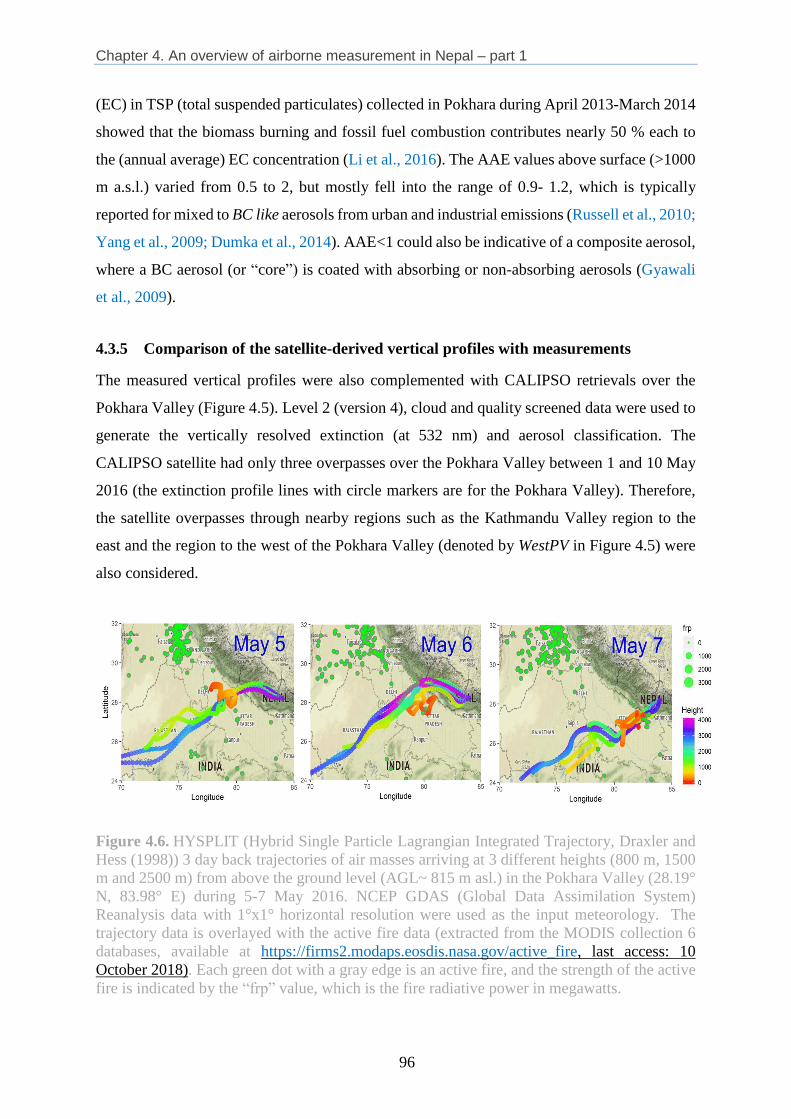
Chapter 4. An overview of airborne measurement in Nepal – part 1
96
(EC) in TSP (total suspended particulates) collected in Pokhara during April 2013-March 2014
showed that the biomass burning and fossil fuel combustion contributes nearly 50 % each to
the (annual average) EC concentration (Li et al., 2016). The AAE values above surface (>1000
m a.s.l.) varied from 0.5 to 2, but mostly fell into the range of 0.9- 1.2, which is typically
reported for mixed to BC like aerosols from urban and industrial emissions (Russell et al., 2010;
Yang et al., 2009; Dumka et al., 2014). AAE<1 could also be indicative of a composite aerosol,
where a BC aerosol (or “core”) is coated with absorbing or non-absorbing aerosols (Gyawali
et al., 2009).
4.3.5 Comparison of the satellite-derived vertical profiles with measurements
The measured vertical profiles were also complemented with CALIPSO retrievals over the
Pokhara Valley (Figure 4.5). Level 2 (version 4), cloud and quality screened data were used to
generate the vertically resolved extinction (at 532 nm) and aerosol classification. The
CALIPSO satellite had only three overpasses over the Pokhara Valley between 1 and 10 May
2016 (the extinction profile lines with circle markers are for the Pokhara Valley). Therefore,
the satellite overpasses through nearby regions such as the Kathmandu Valley region to the
east and the region to the west of the Pokhara Valley (denoted by WestPV in Figure 4.5) were
also considered.
Figure 4.6. HYSPLIT (Hybrid Single Particle Lagrangian Integrated Trajectory, Draxler and
Hess (1998)) 3 day back trajectories of air masses arriving at 3 different heights (800 m, 1500
m and 2500 m) from above the ground level (AGL~ 815 m asl.) in the Pokhara Valley (28.19°
N, 83.98° E) during 5-7 May 2016. NCEP GDAS (Global Data Assimilation System)
Reanalysis data with 1°x1° horizontal resolution were used as the input meteorology. The
trajectory data is overlayed with the active fire data (extracted from the MODIS collection 6
databases, available at https://firms2.modaps.eosdis.nasa.gov/active_fire, last access: 10
October 2018). Each green dot with a gray edge is an active fire, and the strength of the active
fire is indicated by the “frp” value, which is the fire radiative power in megawatts.

Chapter 4. An overview of airborne measurement in Nepal – part 1
97
The range of extinction values for the Pokhara Valley (0.15-0.25 km-1 especially around 2000-
4000 m asl.) were similar to pre-monsoon values (0.15-3 km-1) reported in Nainital (a hilly
station located ~2000 m (asl.) in India, and 400 km west of the Pokhara Valley) and slightly
less than Kanpur, a site in the IGP, about 400 km to the southwest of Pokhara (Dumka et al.,
2014). A large extinction (>0.5 km-1) was observed on 1 May 2016 over the Pokhara Valley at
an altitude of 3-4 km (asl.) which can be attributed to smoke (biomass- related) and polluted
dust (a mixture of dust and biomass smoke or urban pollution) as evident by the aerosol type
classification. Aerosols over the IGP and in the proximity of the Himalayan foothills were
mainly “Dust” on 1 May 2016. Although not conclusive, the 9 May aerosol type classification
is markedly different from 1 May with the absence of dust in the IGP, and absence of polluted
dust or smoke over the Pokhara Valley.
4.3.6 Role of synoptic circulation in modulating aerosol properties over the Pokhara
Valley
The measured vertical profiles and available satellite data from MODIS (See Figure B.8) and
CALIPSO suggest that the synoptic-scale circulations were changing during the study period.
The changing synoptic circulation also influenced the transport of polluted air into the Pokhara
Valley. The regional meteorology station in the Pokhara Valley reported hazy conditions till 5
May 2016(see Figure B.6) which disappeared from 6 May 2016 onwards followed by clear
days with scattered clouds during the daytime and thunderstorms in the afternoon. The
variation in the AOD, AOD-F and Fine Mode Fraction (FMF) from AERONET (only level 1.5
data were available, see Figure B.7) also showed that high turbidity in the atmospheric column,
dominated by fine-mode aerosols before 5 May 2016 (AOD500nm>2.0, FMF >0.9), which
declined sharply after 5 May 2016. The variation in the horizontal visibility (or visual range)
measured at the meteorology station in the Pokhara Valley further indicates that the intensity
of pollution declined during the study period, especially starting on 5 May 2016.
Three day back trajectories (72 h) were generated using HYSPLIT (Hybrid Single Particle
Lagrangian Integrated Trajectory) for air masses arriving in the Pokhara Valley at 800 m, 1,500
m and 2,500 m from above ground level (agl.) for the test flight period (see Figure 6). The
NCEP GDAS reanalysis data with a 1°x1° horizontal resolution were used as the input
meteorology for the trajectories. The majority of air masses (especially at 1500 and 2000 m
agl.) were westerly. A high resolution (0.0625° horizontal) simulation of air mass trajectories
during the pre-monsoon period over the Himalayas and Tibetan Plateau region by Lüthi et al.

Chapter 4. An overview of airborne measurement in Nepal – part 1
98
(2015) also identified synoptic-scale transport (as westerly advection around 500 mb) and a
convection-enabled polluted airmass from the IGP as a major mechanism of transport of air
pollution in the Himalayas. Transport of air pollution by both mechanisms was coupled with
the diurnal expansion of PBL height in the IGP where the trajectory height was similar to
planetary boundary layer (PBL) height thus allowing mixing up of the polluted layer, also
observed by Raatikainen et al. (2014) over Gual Pahari (IGP site) and Mukteswor (Himalayan
foothill site).
During the study period, the direction of the trajectories varied as the air masses entered Nepal
and eventually into the Pokhara Valley. On 5 and 6 May 2016, the air masses (at 1500 and
2000 m a gl.) were mostly northwesterly traversing through northern India and western Nepal
before entering the Pokhara Valley. A shift in the trajectory direction from north westerly to
south westerly was observed on 7 May 2016, where the trajectories were moving through
central India and the southern foothills into the Pokhara Valley. The observed shift in the
trajectories at 1500 and 2500 m AGL was modulated by the synoptic-scale changes in the mid-
latitude (over Central Asia) air masses (40-50° N) (Lüthi et al., 2015). The intrusion (in the
form of a trough) of the cold and humid air masses from 40-50° N (see Figure 2) into 20-30°
N occurred during the study period. As the trough moves eastward, it shifts the synoptic air
mass at 20-30° N from northwesterly to southwesterly on 7 May 2016. The elevated polluted
layer on 5 and 6 May 2016 (Figure 4.4) could be the result of this modulation of the westerly.
The northwesterly airmass entered Nepal via Northern India, where MODIS retrievals showed
a high aerosol loading (See Figure B.8), which could be mainly attributed to the numerous
biomass fire events (See Figure B.9) observed in North India. In addition, numerous forest
fires were also reported in western Nepal during the same period. However, the absorption
signal from the flight measurement does not clearly show higher absorption at shorter
wavelengths compared to absorption at 880 nm or longer wavelengths. This also implies that
the observed elevated polluted layer in the Pokhara Valley is not entirely due to the biomass
burning plume intercepted by the westerlies or north-westerlies. As the airmass origin shifts to
southwesterly on 7 May 2016 (detected during flight F5), the synoptic air mass bypassed the
high AOD loading over north India and contained the cold and relatively clean air from Central
Asia. This resulted in the disappearance of the polluted layer over 2000 m asl. during flight F5.

Chapter 4. An overview of airborne measurement in Nepal – part 1
99
4.4 Conclusion
This paper provides an overview of the pre-monsoon airborne measurement carried out with a
microlight aircraft platform in the Pokhara Valley in Nepal, the first-of-their-kind airborne
aerosol measurements in the Himalayan foothill region. The objective of the overall airborne
campaign in the Himalayan region was to quantify the vertical distribution of aerosols over a
polluted mountain valley region, as well as to measure the extent of regional transport into the
Himalayas. In this paper, measurements from the test flights during May 2016 are summarized.
These mainly include vertical profiles of aerosol number and size distribution, multi-
wavelength aerosol absorption, black carbon, total particle concentration, and meteorological
variables. The instrument package, designed for a microlight sampling was fitted to an
IKARUS-C42 microlight aircraft. A total of five test flights were conducted between 5 and 7
May 2016, including morning and evening flights for about 1-1.5 h each, as well as vertical
spirals to characterize vertical profiles of aerosols and meteorological parameters
The results presented in this paper should be considered as a pilot study mapping out the aerosol
concentrations and their interactions with meteorological processes in the Pokhara Valley due
to the limited flight time. In all the measured flights, the vertical profiles of aerosol parameters
showed strong gradients along the atmospheric column. The observed total number
concentration gradient was strongly influenced by the mountain valley boundary layer, which
resulted in a sharp gradient below about 1500-2000 m (asl.). The increase of boundary layer
height contributed to the differences in the morning and afternoon profiles. Similar vertical
profiles of BC concentrations and aerosol total particle number concentrations provided
evidence of common emission sources or co-located origins. The observed BC concentration
near the surface (~ 1000 m asl.) was much lower than pre-monsoon BC concentrations
measured in the Kathmandu Valley but comparable to values reported during the winter season
in Kanpur in the IGP. The AAE estimates near the surface, based on the absorption value, fell
in the range of 0.9-1.2, which indicates the presence of BC like and mixed (dust, urban,
biomass) aerosols. An elevated polluted layer was observed at around 3 km (asl.) over the
Pokhara Valley during this study. Characterized by a strong presence of dust in the IGP and
polluted continental airmasses over the Pokhara Valley, the polluted layer could be linked with
the westerly synoptic circulations and regional transport from the IGP and surrounding regions.
The direction of the synoptic transport entering the Himalayan foothills and into Pokhara
Valley, however, was influenced by the Westerlies at mid-latitudes (40-50° N). The extent of
transport can be better quantified with regional airborne measurements along the south-north

Chapter 4. An overview of airborne measurement in Nepal – part 1
100
transect through the region between the IGP and the Himalayan foothills at high altitudes in
the Himalayas, including the Pokhara Valley. We will explore the extent of such regional
transport in a subsequent publication that will be primarily based on the airborne measurements
in phase II (December 2016- January 2017) in the Pokhara Valley and in the surrounding
region. The subsequent paper will also characterize the extent of vertical transport from three
different mountain valleys located at different elevations along the south-north transect.

Chapter 5. Discussion and conclusions
101
Chapter 5
5 Discussion and Conclusions
5.1 Overview and key messages
As reported and analyzed using the data in this thesis, and in many past studies noted herein,
the atmosphere of the Kathmandu Valley is highly polluted (Mahata et al., 2018; Shakya et al.,
2017; Chen et al., 2015; Putero et al., 2015; Sarkar et al., 2015; Gurung et al., 2013), which is
characteristic of much of the Himalayan region, as well as most of southern Asia. This air
pollution has many impacts, on health, climate, agriculture, tourism and other sectors (Wester
et al., 2019; WHO, 2016), which could potentially be mitigated to a large extent through
various measures, many of which are readily available (e.g., better combustion
technologies). In order to suggest appropriate measures to focus on for mitigating the local
and/or regional impacts of air pollutants, of course, a greater knowledge base is needed,
especially about the key pollutants and their distributions, seasonality and sources. This is
where this thesis contributes. We achieve this by addressing three important issues: (i) temporal
characteristics (daily, monthly, and seasonal) of two important GHGs in air, CO2 and CH4, and
two key gaseous air pollutants, CO and O3, (ii) spatial distributions of CO and O3, and (iii)
vertical distribution of particles (particulate matter, PM, and especially black carbon, BC) in
the foothills of the central Himalaya. The first study (paper 1 as presented in Chapter 2) based
on research questions (RQ) 1 and 2 (mentioned in the Introduction chapter) focused on CH4
and CO2 observations in the Kathmandu Valley and surrounding region, which were made as
part of this thesis, which is the first of its kind reporting on the seasonal and temporal behavior
of CH4 and CO2 in the central Himalayan region. The study further explored their possible
emission sources in the Kathmandu Valley and surrounding regions. The second study (paper
2 in Chapter 3), which is also based on RQs 1 and 2, reported, for the first time, temporal
distributions of CO and tropospheric O3 based on simultaneous measurements of these two
gases at multiple sites on the valley floor, on the mountain ridges in the east and west, and at
the only river outlet, in the southwest corner of the valley. It also investigated prevalent local
sources and interactions of emissions with meteorology and the influence of regional sources
associated with mixing ratio increases in recent years in the Kathmandu Valley. Estimating the
CO emission flux using the mixing layer height (MLH) and CO mixing ratios and its

Chapter 5. Discussion and conclusions
102
comparison with currently available regional and global emission inventory datasets is a unique
contribution of this study for the southern Asian region. The third study (paper 3 in Chapter 4)
based on RQs 2 and 3 sheds light on the measurements of aerosol particles (PM, BC and
particle number concentrations) and their vertical distributions in the Pokhara Valley in the
foothills of the central Himalaya. The paper also describes the general meteorology of the
Pokhara Valley during the pre-monsoon season. This study reports the first aerial sampling of
air pollutants in the central Himalayan region.
While comparing the diurnal pattern of major GHGs with CO at the Bode site in the central
Kathmandu Valley, it is observed that the diurnal behaviors of the CH4 and CO2 mixing ratios
are found to be different from that of CO, which shows pronounced peaks in the morning and
evening hours and a dip in the afternoon period (Figure 7, Mahata et al., 2017), similar to
Panday et al. (2009). However, CH4 and CO2 show morning peaks, low afternoon values and
again a general rise in the evening until the morning peak on the following day. Another
important observation is a 1-2 hour delay in the morning peaks of CO at Bhimdhunga
(mountain ridge on the west) and Naikhandi (river outlet in the southwestern corner of the
Valley) compared to Bode in the central Kathmandu Valley. This indicates that the city
pollution is influencing the morning peak of the outskirt sites Bhimdhunga and Naikhandi due
to upslope winds and the wind channeled through the Bagmati River outlet, respectively, after
the radiative heating of the surface in the morning (Mahata et. al., 2018, Mues et al., 2017).
The mixing ratios of CH4, CO2 and CO are minimum in the afternoon (from 12:00 to 15:00
local time) due to the active circulation after the dissolution of the nocturnal stable layer and
the increase in daytime MLH (Mues et al., 2017).
The main local emission sources which play important roles for pollutants and GHGs in the
Kathmandu Valley are the transport sector, the residential sector, industries (mainly the brick
industry) and waste burning. Furthermore, the bowl-shaped topography of the valley is also
responsible for high mixing ratios during peak hours due to the low MLH. The recirculation of
emitted species, which have spent one night in the elevated layer, partly enhances the mixing
ratios of air pollutants and GHGs during the morning peak (Panday and Prinn, 2009; Panday
et al., 2009). Furthermore, the mixing ratios of CH4, CO2 and CO are significantly influenced
by several different sources in different seasons, such as the brick industries from January to
April (Mahata et al., 2018; Mahata et al., 2017; Mues et al., 2017; Kim et al., 2016; Chen et
al., 2015; Sarkar et al., 2015). The CO/CO2 ratio analysis also indicated that the brick industries

Chapter 5. Discussion and conclusions
103
are major polluting sources in winter in the valley (Mahata et al., 2017). This result is similar
to Kim et al. (2016) who looked into PM2.5, OC and EC and Sarkar et al. (2015) who studied
NMVOCs. Another important emission source is open trash burning that is quite common
during the winter season. Moreover, the forest fires and agricultural residue burning in the
region (including IGP) play important roles, increasing the mixing ratio of these species during
the pre-monsoon season (Bhardwaj et al., 2018; Mahata et al., 2018; Putero et al., 2015). The
ultralight flight measurement and long-term AERONET observations in the Pokhara Valley
have also reported similar results of high AOD values in the pre-monsoon season when the
wind direction is from the polluted region of the Indo-Gangetic Plain (Singh et al., 2019).
Similarly, there are large changes in CO mixing ratios during episode days compared to normal
days at Bhimdhunga and Naikhandi (outskirt sites), especially relative to the changes observed
at Bode (Mahata et al., 2018). This indicated the contribution of regional emissions to the
pollutants in the Kathmandu Valley. The higher O3 mixing ratios at Nagarkot (hill site) (Mahata
et al., 2018) also indicated regional-scale O3 pollution.
Long-term (greater than a year) CH4 and CO2 observations at Bode and 3 months of
simultaneous observations of these gases at Chanban, outside the Valley, are first of their kind
in the central Himalayan region. The analyzed seasonality and diurnal variation of CH4 and
CO2 at the two sites will be useful for evaluation of model simulations of the region. The
comparison of CH4 and CO2 at Bode and Chanban shows the influence of urbanization at Bode,
which provides useful information about the impacts of urban development. In contrast, the
mixing ratios of CH4, CO2 and CO at Chanban are consistent with the baseline mixing ratios
of these species in the Kathmandu Valley (Figure 2.10, Mahata et al., 2017), and thus can be
considered as representative of the broader regional values.
Our study is not only focused on the spatial and temporal behavior of GHGs and air pollutants;
we have also estimated CO emission flux in the Kathmandu Valley. The calculation of the CO
emission flux was based on the observed CO mixing ratios and the MLH while it is near-
constant at night, similar to what was done for BC in Mues et al. (2017). This is one of the
unique contributions of this study (as also highlighted in the open access review of the paper
by referee 2), providing insights into CO emissions in source regions like the Kathmandu
Valley in the southern Asian region (Mahata et al., 2018). Although there are some limitations
in calculating the CO emission flux by using MLH and CO mixing ratios, the estimated flux
values in this study are 2-14 times higher than the values in widely-used global and regional

Chapter 5. Discussion and conclusions
104
emission databases (EDGAR HTAP, REAS and INTEX-B) (Mahata et al., 2018). Mues et al.
(2017), using the same method, also found a similar underestimation of BC emission fluxes.
This indicates that there is a need for a more detailed emission inventory for CO and BC (and
perhaps for other species as well) for the region.
Furthermore, this thesis also analyzed tropospheric O3, an important gaseous air pollutant and
GHG. The simultaneous O3 observations at Bode, Paknajol and Nagarkot for a one year period
provided quantitative information on O3, and its spatial, temporal and seasonal distributions in
the Kathmandu Valley. Daily 8-hour maximum O3 exceeded the WHO guideline (50 ppb)
about 80% of the days at all sites during the pre-monsoon season, which is of significant
concern for impacts on health and agriculture in the Kathmandu Valley and surrounding
regions. The high level of O3 in this season is due to extensive photochemical production, the
influence of regional forest fires, and agro-residue burning, along with possible stratospheric
intrusion (Bhardwaj et al., 2018; Mahata et al., 2018; Putero et al., 2015; Cristofanelli et al.,
2010; Pudasainee et al., 2006). Furthermore, daily 8 hour maximum O3 exceeded the WHO
limit for 92 % of the days during the pre-monsoon at the mountain site (Nagarkot), which is
indicative of regional-scale high O3 pollution. Hence, if appropriate mitigation options are not
taken, the 8-hour maximum O3 may end up exceeding the WHO recommended O3 level even
in the post-monsoon and winter season at all sites in the near future, which will have further
adverse impacts on human health and ecosystems.
After publication of the scientific results of the SusKat-ABC campaign (which included the
three papers in this thesis, along with numerous other studies, with several including the data
collected in this thesis), the local and regional science, policy and regulatory communities
(along with other stakeholders) have taken up discussion of these results, and the Government
of Nepal has taken important first steps to address the serious air pollution issue in the country:
National air quality monitoring with an aim of setting up 56 stations across the country.
As of July 2021, there are 26 air quality monitoring stations functional in the country,
including 7 in the Kathmandu Valley.
After the 2015 April earthquake, most of the traditional brick kilns have been re-
constructed using considerably less polluting designs and technologies.
All public vehicles in the country more than 20 years old have been phased out since
18 March 2018 to reduce emission sources.

Chapter 5. Discussion and conclusions
105
The Government of Nepal introduced the Kathmandu Valley air pollution management
action plan in 24 February 2020.
5.2 Conclusions and future priorities
This thesis has made an important contribution to understanding air pollution in the Kathmandu
Valley and Nepal, and by providing a framework for analyzing air pollutants and the effects of
circulation in similar other regions of southern Asia. Related studies, including several which
have made use of the data collected in this thesis, have further helped to fill the gaps in this
area. However much remains to be done in order to be able to really understand the local vs.
the regional air pollution and its impacts and sources.
The conclusions of this thesis, which are based on the three research questions discussed above
are as follows:
Research Question (RQ) 1: CO2 and CH4 (GHGs) and CO (an air pollutant) show distinct
diurnal variations: morning and evening peaks with a dip in the afternoon in the Kathmandu
Valley. The difference observed between two GHGs and CO is in their nighttime
characteristics: CO decreases after an evening peak, while the GHG mixing ratios keep
increasing until the next morning peak in the valley. This behavior of the GHGs is not observed
at the Chanban site. The spatial study of CO and O3 at multiple sites in the Kathmandu Valley
shows the tight connection between meteorology (especially wind speed, wind direction and
temperature) and the pollutants, as evident in the delayed morning peak of CO at the outskirt
sites (Naikhandi and Bhimdhunga) in comparison to Bode. The greater exceedance of daily 8-
hour maximum O3 observed at the hilltop site (Nagarkot) than at the urban/semi-urban sites
corroborates the role of meteorology, topography and regional contributions, with high levels
of ozone partly coming from long-range transport, including from the Indo-Gangetic Plain.
RQ 2: The main local sources of GHGs and air pollutants in the valley are transport, residential
activities, industries and trash burning. The CO/CO2 ratio analysis shows that during the winter
season, brick kilns and vehicles are the dominant sources. Similarly, regional forest fires and
agro-residue burning within Nepal, as well as outside Nepal, especially in the IGP region affect
the mixing ratios of CO and O3 in the Kathmandu Valley during the pre-monsoon season.
RQ 3: The concentration of aerosol particles (PM, BC) decreases with the increasing height up
to 4500 m asl. (The observational limit for the micro-light aircraft used in the study). However,

Chapter 5. Discussion and conclusions
106
an elevated aerosol layer was regularly detected around 3000 m asl. during the flight
measurements. The concentrations of PM and BC in the elevated layer are similar to their
concentrations near the surface (ca. 800 m asl.) over the Pokhara Valley. The elevated aerosol
layer, which contributes to the maximum AOD observed at Pokhara Valley during the pre-
monsoon season, is primarily due to the transport of dust and other aerosol particles including
forest fire emissions in the foothill region) by westerly advection from the IGP to the foothills
of the Himalaya and the mountain valleys.
In order for the Government of Nepal to be able to develop effective, concrete plans and
policies to mitigate GHGs and air pollution within Nepal, several steps will be needed. A more
detailed knowledge of the regional O3 chemistry is lacking; in particular, detailed knowledge
of the O3 precursors (NOX and VOCs), especially distinguishing into either NOx or VOC
dominated regimes, along with the regional meteorology in the valley is required. Achieving
this would require long-term simultaneous monitoring of O3 and key precursors at several
places within the valley.
Thus, a final aspect to consider is the regional contribution to the air pollutants and GHGs in
the Kathmandu Valley, as well as in other parts of the central Himalayan region, and how these
could be more effectively mitigated. In particular, dedicated studies of source apportionment
of regional emission sources will be helpful for policy makers to make better plan for
improving air quality in the valley. Among the various pollutants, I would place the greatest
emphasis on mitigation of O3, since there is less awareness of it as a pollutant than PM, which
already receives enhanced attention because it reduces visibility. Thus, we need to study O3
chemistry and its precursors within the valley and surroundings, as well as regional
contributions to O3 in the valley, in order to develop effective science-informed mitigation
options.

Appendix A. SI: Seasonal and diurnal variations in methane and carbon dioxide
107
Appendix A
Supporting Information:
Seasonal and Diurnal Variations of Methane and Carbon Dioxide
in the Kathmandu Valley in the Foothills of the Central Himalaya
Figure A.1. Correlation between hourly CO mixing ratios measured simultaneously with a
cavity ring down spectrometer (Picarro G2401, USA) and a CO analyzer (Horriba AP370,
USA) at Bode, a semi-urban site in the Kathmandu Valley during 6 March to 7 June 2013.

Appendix A. SI: Seasonal and diurnal variations in methane and carbon dioxide
108
Figure A.2. Diurnal variation of hourly average wind directions in different seasons; (a) pre-
monsoon, (b) monsoon, (c) post-monsoon, and (d) winter season observed at Bode for a year
(06 Mar 2013- 04 Mar 2014). Seasons are defined as Pre-monsoon: Mar-May, Monsoon: Jun-
Sep, Post-monsoon: Oct-Nov, Winter: Dec-Feb. The lower and upper end of the whisker
represents 10th and 90th percentile, respectively; the lower end and upper end of each box
represents 25th and 75th percentile, respectively, and black horizontal line in the middle of each
box is the median for each month. The information on the box and whisker is same for Figure
A3.

Appendix A. SI: Seasonal and diurnal variations in methane and carbon dioxide
109
Figure A.3. Diurnal variation of hourly average wind speeds in different seaasons; (a) pre-
monsoon, (b) monsoon, (c) post-monsoon and (d) winter season observed for a year (06 Mar
2013- 05 Mar 2014) at Bode.

Appendix A. SI: Seasonal and diurnal variations in methane and carbon dioxide
110
Figure A.4. Time series of hourly average ambient temperature, wind speed, pressure, and
rainfall observed at Chanban, a rural site outside the Kathmandu Valley from 15 July to 03
October 2015.

Appendix B. SI: An overview of airborne measurement in Nepal – part 1
111
Appendix B
Supplementary Information:
An Overview on the Airborne Measurement in Nepal, - Part 1:
Vertical Profile of Aerosol Size - Number, Spectral Absorption
and Meteorology
c
a b
65
o
Grimm OPS (Spectrometer)
Chilled Miller, Dewpoint
DAQ
TSI CPC (Counter)
¼ in
Brass ¼ inch to wing span Separate inlet
c
Figure B.1. Testing and assembly of the instrument package inside IKARUS-C42 in the COMCO
IKARUS station in Germany (a) field station in Pokhara Valley (b) sketch of the Instrument
package (c).

Appendix B. SI: An overview of airborne measurement in Nepal – part 1
112
Figure B.2. Monthly mean values of key meteorological parameters measured at the Pokhara
regional airport (station ID: 804, 28.1993528, 83.9784028, 820-meter altitude) using an
ENVIRODATA weather station. December 2016 is missing due to data availability. The
monthly value of solar radiation shown here is 95 percentiles of the daily values to reflect the
peak insolation values. Wind speed and rainfall intensity are 10x for graphical clarity. Note
that rainfall values presented here are not cumulative over a month, rather average of the month.
(December data is not available).
The annual mean temperature in the valley was 22° C, with the lowest monthly mean in January
(~15° C) and the highest in July (~ 25° C). Rainfall was also highest in the months of August
and September (summer monsoon season), followed by relatively dry post-monsoon (October-
November) and winter period (December-February). The late pre-monsoon to summer
monsoon were also the periods of maximum monthly solar insolation (~900 Wm-2) and the
insolation is approximately half (~550 Wm-2) during the winter.

Appendix B. SI: An overview of airborne measurement in Nepal – part 1
113
Figure B.3. Frequency of wind speed and direction observed in the Pokhara Valley during
May 2016.
Figure B3.1: Wind speed (ms-1) and direction from 5-7 May 2016 measured at the Pokhara
Regional Airport meteorological station.

Ap
pe
nd
ix B
. S
I: A
n o
ve
rvie
w o
f a
irb
orn
e m
easure
me
nt
in N
epa
l – p
art
1
114
Fig
ure
B.4
. D
aily
tem
per
ature
and r
elat
ive
hum
idit
y a
t 500m
b u
sing t
he
NC
EP
NC
AR
rea
nal
ysi
s (2
.5x
2.5
o)
dat
a over
South
Asi
a fr
om
May 1
to 7
2016.

Appendix B. SI: An overview of airborne measurement in Nepal – part 1
115
Figure B.5. Monthly mean value of AOD 500 nm in Pokhara Valley for 2010-2016 (Note:
Level 2 and 1.5 were used).

Appendix B. SI: An overview of airborne measurement in Nepal – part 1
116
Figure B.6. Local Meteorology in the Pokhara Valley from 1-10 May 2016.
Weather condition is coded by individual number (see NOAA
https://www7.ncdc.noaa.gov/CDO/dataproduct for details). Weather condition in the figure is
shown as a black square box. Weather condition of 5 indicate Hazy conditions;17-thurderstorm
but no precipitation; 3-cloud generally forming; 2-sky unchanged
The sky cover is numerically coded as follows:
CLEAR =1, SCATTERED (1/8 TO 4/8) =2, BROKEN-5/8 TO 7/8 =3, OVERCAST=4,
OBSCURED=5, PARTIAL OBSCURATION=6
(Also see NOAA https://www7.ncdc.noaa.gov/CDO/dataproduct for details).
Hazy condition Scattered clouds
Thurderstorm with no precipitation

Appendix B. SI: An overview of airborne measurement in Nepal – part 1
117
S7. Summary of aerosol properties using AERONET measurement from 2010-2016
AERONET measurements (Holben et al., 1998) have been made in the Pokhara Valley since
January 2010. The AERONET station (83.97° N, 28.18° E, 807 m a.s.l.) is approximately 1.1
km southeast from the Pokhara Regional Airport, located in the semi-urban area of Pokhara
City. Cloud-screened and quality assured (level 2) data were used in the study. Gaps in the
level 2 data were supplemented with level 1.5 data. The AERONET retrieval suffers in the
monsoon months (June to September) due to interference by monsoon clouds in the Pokhara
Valley, as indicated by the gap in Figure 4.2.
A combination of direct products such as aerosol optical depth (AOD) and inversion products
such as fine AOD, absorption Ångstrom exponent (AAE) and volume size distribution were
used for the analysis presented in this study. The typical reported uncertainty in the AERONET
data products for AOD (> 0.04) is approximately ±0.01 to ±0.02, and is higher for shorter
wavelengths (Eck et al., 1999;Holben et al., 1998). The observed uncertainty in AOD also
influences other AERONET products such as the Ångstrom exponent (AE) and the inversion
products. Thus these derived products will have a higher uncertainty than the AOD (Schuster
et al., 2006;Dubovik and King, 2000). Further details about the AERONET direct and inverted
data products can be found in Holben et al. (2006).
In the Pokhara Valley, AOD values showed a strong seasonality in the wavelength bands
between 340 and 1020 nm. The inter-annual variation in the AOD during 2010-2016 was
closely associated with the enhancement in the fine-mode fraction, and to a lesser extent in the
coarse mode for dust (Xu et al., 2014). The observed inter-annual variation in the AOD could
be influenced by the interaction between aerosols and the mesoscale to synoptic-scale
meteorology (Vinoj et al., 2014;Ram et al., 2010;Kaskaoutis et al., 2012a), as well as influences
of the ENSO (El Niño southern oscillation) on West Asia and the IGP (Kim et al., 2016). AOD
values were enhanced or elevated during the winter, with the aerosol load building up
throughout the pre-monsoon months (AOD500nm>0.6, Figure 3a, 3b, and S5) and then falling to
their lowest values in the monsoon months (AOD500nm ~0.2-0.3), most likely due to wet
removal of aerosols. After the low AOD during the monsoon, AOD gradually increases (to
~0.4-0.5) during the post-monsoon through winter to the pre-monsoon season. AOD was
usually highest in April (AOD500nm:0.86±0.36), followed by March, May, and June. The
increase in aerosols load (as reflected by the AOD) during the pre-monsoon months can also
be seen at high altitude sites such as the NCO-P site in the Khumbu Valley near Mt. Everest,
Appendix B. SI: An overview of airborne measurement in Nepal – part 1
118
located at 5057 m (a.s.l.) and about 300 km to the east of Pokhara (see Figure 3c), as well as at
IGP sites in Kanpur (130 m a.s.l., 400 km southwest of the Pokhara Valley) and Gandi Nagar
(60 m a.s.l., 250 km south of the Pokhara Valley). A similar AOD build-up was also observed
by Ram et al. (2010) in Darjeeling (2194 m a.s.l., hill station ~450 km east of Pokhara Valley),
and by Chatterjee et al. (2012) in Manora Peak (1950 m a.s.l., 460 km west of Pokhara Valley).
This regional increase in aerosol load in the IGP and the Himalayan region is partly due to
active transport during the pre-monsoon season, often linked with westerly advection bringing
dust from West Asia and nearby arid regions (Gautam et al., 2011). The relatively dryness with
little precipitation during this period also contributes to the total aerosol load, since washout
will be limited. The AOD peaks occur in different months in these different sites in the IGP
and Himalayas, reflecting the varying influence of local meteorology and increase in the
emission sources such as agriculture residue burning dominated by dominated by fine-mode
particles (Putero et al., 2014).
Fine-mode aerosol particles scatter more at shorter wavelengths (such as 340-500 nm)
compared to 1020 nm (Schuster et al., 2006). The variation in the Ångstrom exponent was not
as definitive as in the AOD values; the Ångstrom exponent was generally below 1 during pre-
monsoon months and above 1 in the post-monsoon and winter months. Ångstrom exponent
values of >1 are generally reported for sources such as biomass burning, fossil fuel combustion
and other primary sources which have a dominant fine-mode fraction. Dust and other coarse-
mode aerosols have Ångstrom exponents less than 1 (Eck et al., 1999). The highest values of
the Ångstrom exponent (at least >1.2) were observed for the post-monsoon observation period,
presumably due to emissions of primary fine-mode aerosol from sources such as open burning
of agriculture, often reported in tshis season especially to the south and southeast of Pokhara
Valley and in the IGP. In addition to the Ångstrom exponent, the temporal variation of AOD
fine and coarse modes (at 500 nm) in Figure 3b and 3c also indicates that fine-mode aerosols
nearly exclusively dominate the atmospheric column during the post-monsoon and winter
seasons. In the pre-monsoon season, in addition to the fine-mode, a substantial fraction of
coarse-mode also exists, which is also observed in the monsoon season. On the nature of
aerosols or bulk composition, Figure 3e shows a simple scatter-plot based on the absorption
and extinction Ångstrom exponents (AAE and EAE at 440-870 nm) which can be used to
indicate the aerosol types (Giles et al., 2011; Giles et al., 2012; Dubovik et al., 2002). These
two parameters describe the spectral dependence or “slope” of aerosols absorption and
extinction at the measured wavelength (Seinfeld and Pandis, 2006). Extinction exponent is a

Appendix B. SI: An overview of airborne measurement in Nepal – part 1
119
proxy for aerosol size, while the absorption exponent is a proxy for absorbing aerosols
including a mixed aerosol. The classification employed by Giles et al. (2011) based on
observations from the IGP AERONET sites defines “Dust” or “Mostly Dust” aerosols within
the range of EAE <0.5 and AAE >2.0 and “Mostly BC like” aerosols with EAE EAE <0.8 and
AAE ~1.0-2.0. Urban/industrial and biomass burning aerosols fall under the “Mostly BC”
category (Dubovik et al., 2002; Giles et al., 2011). The mixed aerosol (“Dust+BC”) centers
around a value of EAE ~0.5 and AAE~1.5. Based on this approximate classification from a
monthly data, the dominant aerosol in the Pokhara Valley is mostly BC like; however, the daily
aerosol characteristics can vary from more mixed to dust-like in the pre-monsoon months, to
more BC-like in the post-monsoon and winter months.

Appendix B. SI: An overview of airborne measurement in Nepal – part 1
120
Figure B.7. The AERONET-based aerosol optical depth and radiative properties in the
Pokhara Valley from 2010 to 2016. Monthly summaries are presented using level 2 collections
and supplemented with level 1.5 for missing data points; (S7a) AOD at seven wavelengths;
(S7b) Inversion products such as fine AOD (AOD-F), coarse AOD (AOD-C), and total AOD
~Dust ~BC like
Sub-micron Super-Super-micron
S7d S7e
S7a
S7b
S7c

Appendix B. SI: An overview of airborne measurement in Nepal – part 1
121
(AOD-T), along with Ångstrom exponent (440-870 nm, magenta line); (S7c) AOD-T for
Kanpur, Gandi Nagar (both IGP sites in India) and the NCO-P site (labeled EVK2-CNR, a high
altitude site in the Khumbu Valley at the base of Mt. Everest); (S7d) Seasonal average of
volume particle size distribution grouped by four seasons (the error bar indicates the standard
deviation, and the uncertainty in the calculated size distribution is close to 20 % in the range
0.2 µm <Dp< 14 µm). The four seasons are classified as winter (DJF: December, January and
February), monsoon (JJAS: June, July, August and September), pre-monsoon (MAM: March,
April and May) and post-monsoon (ON: October and November); (S7e) absorption Ångstrom
exponent (440-870) and extinction Ångstrom exponent (440-870 nm), color-coded for the four
seasons.
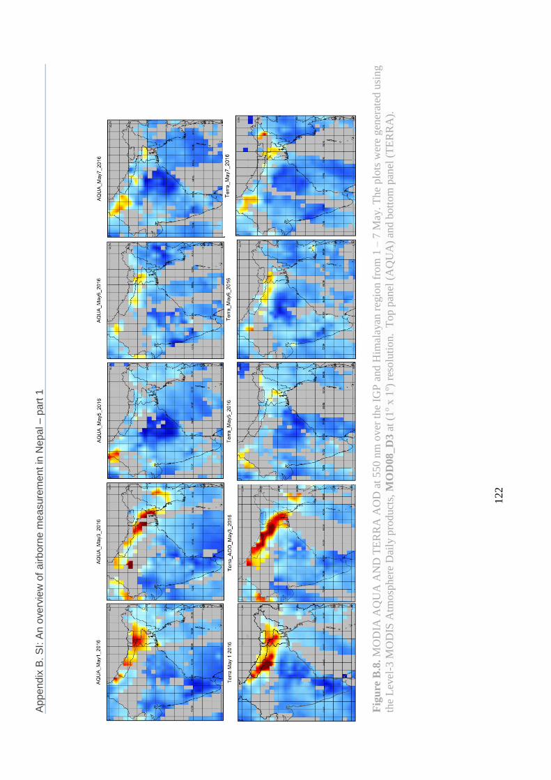
Ap
pe
nd
ix B
. S
I: A
n o
ve
rvie
w o
f a
irb
orn
e m
easure
me
nt
in N
epa
l – p
art
1
122
Fig
ure
B.8
. M
OD
IA A
QU
A A
ND
TE
RR
A A
OD
at
550 n
m o
ver
the
IGP
and
Him
alay
an r
egio
n f
rom
1 –
7 M
ay.
Th
e plo
ts w
ere
gen
erat
ed u
sin
g
the
Lev
el-3
MO
DIS
Atm
osp
her
e D
aily
pro
duct
s, M
OD
08_D
3 a
t (1
o x
1o)
reso
luti
on.
Top p
anel
(A
QU
A)
and b
ott
om
pan
el (
TE
RR
A).

Appendix B. SI: An overview of airborne measurement in Nepal – part 1
123
Figure B.9. Locally or nationally recorded active fire for the same period by the National
Emergency Operation Centre (http://neoc.gov.np/en/) via the ICIMOD portal
(http://118.91.160.238/NepalForestFire/index.html).
Local Fire
Pokhara Valley

Ap
pe
nd
ix B
. S
I: A
n o
ve
rvie
w o
f a
irb
orn
e m
easure
me
nt
in N
epa
l – p
art
1
124
Fig
ure
B.1
0.
Morn
ing t
est
flig
ht
(Fli
ght
F3
) on 6
May
2016 i
s sh
ow
n h
ere,
the
rest
of
the
resu
lts
are
alre
ady s
how
n i
n i
n F
igure
. E
ach
subplo
t is
arra
nged
by (
i) A
eroso
l n
um
ber
siz
e dis
trib
uti
on m
easu
red b
y t
he
Gri
mm
OP
C m
odel
1.1
08 (
0.3
-20 µ
m),
lim
ited
to
1 µ
m i
n t
he
figure
, (i
i) T
ota
l
par
ticl
e num
ber
conce
ntr
atio
n (
also
indic
ated
as
TP
C,
Dp
>11 n
m)
mea
sure
d b
y t
he
TS
I C
PC
3760 a
nd a
bso
rpti
on
aer
oso
l at
370 n
m a
nd 8
80 n
m
(iii
) te
mper
ature
(°C
) an
d d
ew p
oin
t (b
lack
dot,
in °
C)
and
rel
ativ
e hum
idit
y (
or
RH
%),
(iv
) ca
lcula
ted
abso
rpti
on
Ån
gst
rom
ex
ponen
t av
erag
ed
for
ever
y 1
00 m
eter
s el
evat
ion
ban
d.

Appendix B. SI: An overview of airborne measurement in Nepal – part 1
125
Figure B.11. Estimating the AAE value using the power fit and linear fit (left: power fit, right:
linear fit).
y = -0.9667x + 16.416R² = 0.9965
9.675
9.9
10.125
10.35
10.575
6.075 6.3 6.525 6.75 6.975
ln(a
bs_
λ)
ln(λ(nm))
ln(λ) V/S ln(abs_λ)
y = 1E+07x-0.967
R² = 0.9965
0
9000
18000
27000
36000
45000
0 250 500 750 1000
abs_λ
Wavelength (nm)
λ V/S abs_λ
815m Linear Fit
815m Linear Fit 815m Linear Fit
815m Power Fit

Appendix B. SI: An overview of airborne measurement in Nepal – part 1
126
Table T.1
Flight # Flight date Flight time
window
Measured parameter
F1 5 May 2016 7:00-9:00 Morning
flight
T, R, H, total particle count,
number-size distribution, BC
F2 5 May 2016 14:00-17 :00 Afternoon
flight
"
F3 6 May 2016 7:00-9:00 Morning
flight
"
F4 6 May 2016 14:00-17 :00 Afternoon
flight
"
F5 7 May 2016 7:00-9:00 Morning
flight
"

Bibliography
127
Bibliography
Aryal, R. K., Lee, B.-K., Karki, R., Gurung, A., Baral, B., and Byeon, S.-H.: Dynamics of PM
2.5 concentrations in Kathmandu Valley, Nepal, J. Hazard. Mat., 168, 732-738, 2009.
Aryal, D., Rosoff, Y. N., and Devkota, L. P.: A Severe Hailstorm at Pokhara: CAPE Stability
Index Calculations, Journal of Geosciences and Geomatics, 3, 142-153,
Automotive Research Association of India (ARAI).: Emission factor development for Indian
vehicles (http://www.cpcb.nic.in/Emission_Factors_Vehicles.pdf), 2008.
Avnery, S., Mauzerall, D. L., Liu, J., and Horowitz, L. W.: Global crop yield reductions due to
surface ozone exposure: 1. Year 2000 crop production losses and economic damage, Amos.
Environ., 45, 2284–2296, doi:10.1016/j.atmosenv.2010.11.045, 2011.
Bhardwaj, P., Naja, M., Rupakheti, M., Panday, A. K., Kumar, R., Mahata, K., Lal, S.,
Lawrence, M. G., Chandola, H. C.: Variations in surface ozone and CO in the Kathmandu
Valley during SusKat-ABC international field campaign, Atmos. Chem. Phys., 18, 11949–
11971, 2018, https://doi.org/10.5194/acp-18-11949-2018.
Bollasina, M. A., Ming, Y., and Ramaswamy, V.: Anthropogenic Aerosols and the
Weakening of the South Asian Summer Monsoon, Science, 334, 502-505,
10.1126/science.1204994, 2011.
Bonasoni P., P. Laj, A. Marinoni, M. Sprenger, F. Angelini, J. Arduini, U. Bonafè, F. Calzolari,
T. Colombo, S. Decesari, C. Di Biagio, A. G. di Sarra, et al.: Atmospheric brown clouds
in the Himalayas: first two years of continuous observations at the Nepal Climate
Observatory-Pyramid (5079 m). Atmos. Chem. Phys., 10, 7515-7531, 2010.
Brauer, M., Amman, M., Burnett, R. T., Cohen, A., Dentener, F., Zenati, M., Henderson, S. B.,
Krzyzanowski, M., Martin, R. V., Van Dingenen, R., van Donkelaar, A., and Thurston, G.
D.: Exposure assessment for estimation of the global burden of disease attributable to
outdoor air pollution, Environ. Sci. Technol., 46, 652–660, doi:10.1021/es2025752, 2012.
Brun, V. (Eds. 1): Fried earth bricks, kilns and workers in Kathmandu Valley. Himal Books,
Lazimpat-Kathmandu, Nepal, 2013.
Burney, J., and Ramanathan, V.: Recent climate and air pollution impacts on Indian agriculture,
Proceedings of the National Academy of Sciences of the United States of America, 111,
16319-16324, doi:10.1073/pnas.1317275111, 2014.

Bibliography
128
Central Bureau of Statistics (CBS): Nepal Living Standards Survey 2010/11, Statistical Report
Volume 1, Central Bureau of Statistics, Government of Nepal, 2011.
Chandra, N., Lal, S., Venkataramani, S., Patra, P. K., and Sheel, V.: Temporal variations of
atmospheric CO 2 and CO at Ahmedabad in western India, Atmos. Chem. Phys., 16, 6153-
6173, 2016.
Chang K-L, Petropavlovskikh I, Cooper OR, Schultz MG, Wang T.: Regional trend analysis
of surface ozone observations from monitoring networks in eastern North America, Europe
and East Asia. Elem Sci Anth., DOI:http://doi.org/10.1525/elementa.243, 2017.
Chen, H., Karion, A., Rella, C., Winderlich, J., Gerbig, C., Filges, A., Newberger, T., Sweeney,
C., and Tans, P.: Accurate measurements of carbon monoxide in humid air using the cavity
ring-down spectroscopy (CRDS) technique, Atmos. Meas. Tech., 6, 1031-1040, 2013.
Chen, P., Kang, S., Li, C., Rupakheti, M., Yan, F., Li, Q., Ji, Z., Zhang, Q., Luo, W., and
Sillanpää, M.: Characteristics and sources of polycyclic aromatic hydrocarbons in
atmospheric aerosols in the Kathmandu Valley, Nepal, Sci. Total Environ., 538, 86-92,
2015.
Chen, Y. H., and Prinn, R. G.: Estimation of atmospheric methane emissions between 1996
and 2001 using a three‐dimensional global chemical transport model, J. Geophys. Res.
Atmos., 111, 2006.
Cho, C., Kim, S. W., Rupakheti, M., Park, J. S., Panday, A., Yoon, S. C., Kim, J. H., Kim,
H., Jeon, H., Sung, M., Kim, B. M., Hong, S. K., Park, R. J., Rupakheti, D., Mahata, K.
S., Praveen, P. S., Lawrence, M. G., and Holben, B.: Wintertime aerosol optical and
radiative properties in the Kathmandu Valley during the SusKat-ABC field campaign,
Atmos. Chem. Phys., 17, 12617-12632, 10.5194/acp-17-12617-2017, 2017.
Cong, Z., Kawamura, K., Kang, S., and Fu, P.: Penetration of biomass-burning emissions
from South Asia through the Himalayas: new insights from atmospheric organic acids, 5,
9580, 10.1038/srep09580
http://dharmasastra.live.cf.private.springer.com/articles/srep09580#supplementary-
information, 2015.
Conrad, R.: Soil microorganisms as controllers of atmospheric trace gases (H2, CO, CH4,
OCS, N2O, and NO), Microbiol.Rev., 60, 609-640, 1996.
Cristofanelli, P., Bracci, A., Sprenger, M., Marinoni, A., Bonafè, U., Calzolari, F., Duchi, R.,
Laj, P., Pichon, J. M., Roccato, F., Venzac, H., Vuillermoz, E., and Bonasoni, P.:
Tropospheric ozone variations at the Nepal Climate Observatory- Pyramid (Himalayas,

Bibliography
129
5079ma.s.l.) and influence of deep stratospheric intrusion events, Atmos. Chem. Phys., 10,
6537–6549, doi:10.5194/acp-10-6537-2010, 2010.
Crosson, E.: A cavity ring-down analyzer for measuring atmospheric levels of methane, carbon
dioxide, and water vapor, Appl. Phys. B: Lasers and Optics, 92, 403-408, 2008.
Davidson, C. I., Lin, S.-F., and Osborn, J. F.: Indoor and outdoor air pollution in the Himalayas,
Environ. Sci. Technol., 20(6), 561 – 566, doi:10.1021/es00148a003, 1986.
Department of Transport Management (DoTM).: Annual report of Ministry of Labor and
transport management, Nepal Government, 2015.
Decesari, S., Facchini, M. C., Carbone, C., Giulianelli, L., Rinaldi, M., Finessi, E., Fuzzi, S.,
Marinoni, A., Cristofanelli, P., Duchi, R., Bonasoni, P., Vuillermoz, E., Cozic, J., Jaffrezo,
J. L., and Laj, P.: Chemical composition of PM<sub>10</sub> and PM<sub>1</sub> at
the high-altitude Himalayan station Nepal Climate Observatory-Pyramid (NCO-P) (5079
m a.s.l.), Atmos. Chem. Phys., 10, 4583-4596, 10.5194/acp-10-4583-2010, 2010.
Deb Roy, S., Beig, G., Ghude, S.D.: Exposure-plant response of Ambient ozone over the
tropical India region. Atmos. Chem. Phys. 9, 5253e5260, 2009.
Dentener, F., Stevenson, D., Ellingsen, K., Van Noije, T., Schultz, M., Amann, M., Atherton,
C., Bell, N., Bergmann, D., and Bey, I.: The global atmospheric environment for the next
generation, Environ. Sci. Technol., 40, 3586-3594, 2006.
Dey, S., and Di Girolamo, L.: A climatology of aerosol optical and microphysical properties
over the Indian subcontinent from 9 years (2000–2008) of Multiangle Imaging
Spectroradiometer (MISR) data, Journal of Geophysical Research: Atmospheres, 115, n/a-
n/a, 10.1029/2009JD013395, 2010.
Dhungel, S., Kathayat, B., Mahata, K., and Panday, A.: Transport of regional pollutants
through a remote trans-Himalayan valley in Nepal, Atmos. Chem. Phys., 18, 1203-1216,
https://doi.org/10.5194/acp-18-1203-2018, 2018.
Dlugokencky, E.J., A.M. Crotwell, P.M. Lang, J.W. Mund, Atmospheric Methane Dry Air
Mole Fractions from quasi-continuous measurements at Mauna Loa, Hawaii, 1986-2016,
Version: 2017-01-20, path: ftp://aftp.cmdl.noaa.gov/data/trace_gases/ch4/in-situ/surface/,
2017.
Dlugokencky, E.J., Lang, P.M., Crotwell, A. M., Mund, J. W., Crotwell, M. J., and Thoning,
K. W.: Atmospheric Methane Dry Air Mole Fractions from the NOAA ESRL Carbon Cycle
Cooperative Global Air Sampling Network, 1983-2015, Version: 2016-07-07, Path:
ftp://aftp.cmdl.noaa.gov/data/trace_gases/ch4/flask/surface/, 2016.

Bibliography
130
Dlugokencky, E.J., Lang, P.M., Mund, J.W., Crotwell, A. M., Crotwell, M. J., and Thoning,
K. W.: Atmospheric Carbon Dioxide Dry Air Mole Fractions from the NOAA ESRL
Carbon Cycle Cooperative Global Air Sampling Network, 1968-2015, Version: 2016-08-
30, Path: ftp://aftp.cmdl.noaa.gov/data/trace_gases/co2/flask/surface/, 2016a.
Draxler, R. R., and Hess, G. D.: An overview of the HYSPLIT_4 modeling system for
trajectories, dispersion, and deposition, Aust. Meteor. Mag, 47, 295–230, 1998.
Dumka, U. C., N. Tripathi, S., Misra, A., Giles, D. M., Eck, T. F., Sagar, R., and Holben, B.
N.: Latitudinal variation of aerosol properties from Indo-Gangetic Plain to central
Himalayan foothills during TIGERZ campaign, Journal of Geophysical Research:
Atmospheres, 119, 4750-4769, 10.1002/2013jd021040, 2014.
EDGAR42FT: Global emissions EDGAR v4.2FT2010, available at
http://edgar.jrc.ec.europa.eu/overview.php?v=42FT2010, last access: October 2013.
Feng, Z., Hu, E., Wang, X., Jiang, L., Liu, X.: Ground-level O3 pollution and its impacts on
food crops in China: A review, Environ. Pollut., 199, 42-24,
https://doi.org/10.1016/j.envpol.2015.01.016, 2015.
Forouzanfar, M. H., Alexander, L., Anderson, H. R., Bachman, V. F., Biryukov, S., Brauer,
M., Burnett, R., Casey, D., Coates, M. M., and Cohen, A.: Global, regional, and national
comparative risk assessment of 79 behavioural, environmental and occupational, and
metabolic risks or clusters of risks in 188 countries, 1990–2013: a systematic analysis for
the global burden of disease study 2013, Lancet, 386, 2287-2323, doi: 10.1016/S0140-
6736(15)00128-2, 2015.
Fowler, D., Flechard, C., Cape, J. N., Storeton-West, R. L., and Coyle, M.: Measurements of
ozone deposition to vegetation quantifying the flux, the stomatal and nonstomatal
components, Water Air Soil Pollut., 130, 63–74, doi:10.1023/a:1012243317471, 2001.
Fragkias, M., Lobo, J., Strumsky, D., and Seto, K. C.: Does size matter? Scaling of CO2
emissions and US urban areas, PLoS One, 8, e64727, 2013.
Fueglistaler, S., Dessler, A. E., Dunkerton, T. J., Folkins, I., Fu, Q., and Mote, P. W.:
Tropical tropopause layer, Rev. Geophys., 47, RG1004, doi:10.1029/2008RG000267,
2009.
Ganesan, A., Chatterjee, A., Prinn, R., Harth, C., Salameh, P., Manning, A., Hall, B., Mühle,
J., Meredith, L., and Weiss, R.: The variability of methane, nitrous oxide and sulfur
hexafluoride in Northeast India, Atmos. Chem. Phys., 13, 10633-10644, 2013.

Bibliography
131
Gautam, R., Hsu, N. C., Lau, K. M., and Kafatos, M.: Aerosol and rainfall variability over the
Indian monsoon region: distributions, trends and coupling, Ann. Geophys., 27, 3691-3703,
10.5194/angeo-27-3691-2009, 2009a.
Gautam, R., Hsu, N. C., Lau, K. M., Tsay, S. C., and Kafatos, M.: Enhanced pre-monsoon
warming over the Himalayan-Gangetic region from 1979 to 2007, Geophysical Research
Letters, 36, n/a-n/a, 10.1029/2009GL037641, 2009b.
Gautam, R., Hsu, N. C., Tsay, S. C., Lau, K. M., Holben, B., Bell, S., Smirnov, A., Li, C.,
Hansell, R., Ji, Q., Payra, S., Aryal, D., Kayastha, R., and Kim, K. M.: Accumulation of
aerosols over the Indo-Gangetic plains and southern slopes of the Himalayas: distribution,
properties and radiative effects during the 2009 pre-monsoon season, Atmospheric
Chemistry and Physics, 11, 12841-12863, 10.5194/acp-11-12841-2011, 2011.
Geiß, A., Wiegner, M., Bonn, B., Schäfer, K., Forkel, R., von Schneidemesser, E., Münkel, C.,
Chan, K. L., and Nothard, R.: Mixing layer height as an indicator for urban air quality?,
Atmos. Meas. Tech. Discuss., 2017, 1-32, doi:10.5194/amt-2017-53, 2017.
Ghude, S.D., Jain, S.L., Arya, B.C., Beig, G., Ahammed, Y.N., Kumar, A., Tyagi, B.: Ozone
in ambient air at a tropical megacity, Delhi: characteristics, trends and cumulative ozone
exposure indices, J. Atmos. Chem., 60: 237, https://doi.org/10.1007/s10874-009-9119-4,
2008.
Ghude, S. D., Jena, C., Chate, D. M., Beig, G., Pfister, G. G., Kumar, R., and Ramanathan, V.:
Reductions in India’s crop yield due to ozone, Geophys. Res. Lett., 41, 5685–5691,
doi:10.1002/2014GL060930, 2014.
Giles, D. M., Holben, B. N., Eck, T. F., Sinyuk, A., Smirnov, A., Slutsker, I., Dickerson, R. R.,
Thompson, A. M., and Schafer, J. S.: An analysis of AERONET aerosol absorption
properties and classifications representative of aerosol source regions, Journal of
Geophysical Research: Atmospheres, 117, n/a-n/a, 10.1029/2012jd018127, 2012.
Giri, D., Murthy, K., Adhikary, P., Khanal, S.: Ambient air quality of Kathmandu Valley as
reflected by atmospheric particulate matter concentrations (PM10), Int. J. Environ. Sci.
Technol. 3, 403–410, 2006.
Gogoi, M. M., Moorthy, K. K., Kompalli, S. K., Chaubey, J. P., Babu, S. S., Manoj, M. R.,
Nair, V. S., and Prabhu, T. P.: Physical and optical properties of aerosols in a free
tropospheric environment: Results from long-term observations over western trans-
Himalayas, Atmospheric Environment, 84, 262-274,
https://doi.org/10.1016/j.atmosenv.2013.11.029, 2014.

Bibliography
132
Goroshi, S. K., Singh, R., Panigrahy, S., and Parihar, J.: Analysis of seasonal variability of
vegetation and methane concentration over India using SPOT-VEGETATION and
ENVISAT-SCIAMACHY data, J. Indian Soc. Remote, 39, 315-321, 2011.
Guttikunda, S. K., Goel, R., and Pant, P.: Nature of air pollution, emission sources, and
management in the Indian cities, Atmospheric Environment, 95, 501-510,
http://dx.doi.org/10.1016/j.atmosenv.2014.07.006, 2014.
Gyawali, M., Arnott, W. P., Lewis, K., and Moosmüller, H.: In situ aerosol optics in Reno,
NV, USA during and after the summer 2008 California wildfires and the influence of
absorbing and non-absorbing organic coatings on spectral light absorption, Atmos. Chem.
Phys., 9, 8007-8015, 10.5194/acp-9-8007-2009, 2009.
Hansen, A. D. A., Rosen, H., and Novakov, T.: The aethalometer — An instrument for the
real-time measurement of optical absorption by aerosol particles, Science of The Total
Environment, 36, 191-196, https://doi.org/10.1016/0048-9697(84)90265-1, 1984.
Highwood, E. J. and Hoskins, B. J.: The tropical tropopause, Q. J. Roy. Meteorol. Soc., 124,
1579–1604, doi:10.1002/qj.49712454911, 1998.
Huszar, P., Belda, M., and Halenka, T.: On the long-term impact of emissions from central
European cities on regional air quality, Atmos. Chem. Phys., 16, 1331–1352, doi:10.5194/
acp-16-1331-2016, 2016.
International Energy Agency (IEA).: Energy and air pollution, World Energy Outlook Special
Report 2016, International Energy Agency, 2016.
International Centre for Integrated Mountain Development (ICIMOD).: Himalayas – Water for
1.3 Billion People. ICIMOD, Lalitpur, 2009.
Intergovernmental Panel for Climate Change (IPCC).: Climate Change 2013: The Physical
Science Basis. Contribution of Working Group I to the Fifth Assessment Report of the
Intergovernmental Panel on Climate Change, Cambridge University Press, Cambridge,
United Kingdom and New York, NY, USA, 2013.
IPCC: Climate Change 2007: The Physical Science Basis. Contribution of Working Group I to
the Fourth Assessment Report of the Intergovernmental Panel on Climate Change. Chapter
1, Historical Overview of Climate change, in: Intergovernmental Panel on Climate Change
Climate change: The Physical Science Basis, Contribution of Working Group I to the
Fourth Assessment Report of the IPCC, Cambridge University Press, Cambridge, 79–131,
2007.
Jai Devi, J., Tripathi, S. N., Gupta, T., Singh, B. N., Gopalakrishnan, V., and Dey, S.:
Observation-based 3-D view of aerosol radiative properties over Indian Continental

Bibliography
133
Tropical Convergence Zone: implications to regional climate, Tellus B, 63, 971-989,
10.1111/j.1600-0889.2011. 00580.x, 2011.
Janssens-Maenhout, G., Dentener, F., van Aardenne, J., Monni, S., Pagliari, V., Orlandini, L.,
Klimont, Z., Kurokawa, J., Akimoto, H., Ohara, T., Wankmüller, R., Battye, B., Grano, D.,
Zuber, A., and Keating, T.: EDGAR-HTAP: a harmonized gridded air pollution emission
dataset based on national inventories, Tech. Rep. JRC68434, Publications Office of the
European Union, doi:10.2788/14102 (online),
http://publications.jrc.ec.europa.eu/repository/handle/JRC68434, 2000.
Junkermann, W.: An Ultralight Aircraft as Platform for Research in the Lower Troposphere:
System Performance and First Results from Radiation Transfer Studies in Stratiform
Aerosol Layers and Broken Cloud Conditions, Journal of Atmospheric and Oceanic
Technology, 18, 934-946, 10.1175/1520-0426(2001)018<0934:auaapf>2.0.co;2, 2001.
Kaskaoutis, D. G., Singh, R. P., Gautam, R., Sharma, M., Kosmopoulos, P. G., and Tripathi,
S. N.: Variability and trends of aerosol properties over Kanpur, northern India using
AERONET data (2001–10), Environmental Research Letters, 7, 024003, 10.1088/1748-
9326/7/2/024003, 2012.
Kim, B. M., Park, J.-S., Kim, S.-W., Kim, H., Jeon, H., Cho, C., Kim, J.-H., Hong, S.,
Rupakheti, M., and Panday, A. K.: Source apportionment of PM 10 mass and particulate
carbon in the Kathmandu Valley, Nepal, Atmos. Environ., 123, 190-199, 2015.
Kiros, F., Shakya, K. M., Rupakheti, M., Regmi, R. P., Maharjan, R., Byanju, R. M., Naja, M.,
Mahata, K., Kathayat, B., and Peltier, R. E.: Variability of Anthropogenic Gases: Nitrogen
oxides, sulfur dioxide, ozone and ammonia in Kathmandu Valley, Nepal, Aerosol Air Qual.
Res., 16: 3088–3101, 2016.
Kitada, T., and Regmi, R. P.: Dynamics of air pollution transport in late wintertime over
Kathmandu Valley, Nepal: As revealed with numerical simulation, J. Appl. Meteorol., 42,
1770-1798, 2003.
Kuhlmann, J., and Quaas, J.: How can aerosols affect the Asian summer monsoon?
Assessment during three consecutive pre-monsoon seasons from CALIPSO satellite data,
Atmos. Chem. Phys., 10, 4673-4688, 10.5194/acp-10-4673-2010, 2010.
Kumar, M. K., and Nagendra, S. S.: Characteristics of ground level CO2 concentrations over
contrasting land uses in a tropical urban environment, Atmos. Environ., 115, 286-294,
2015.
Kumar, R., Naja, M., Satheesh, S.K., Ojha, N., Joshi, H., Sarangi, T., Pant, P., Dumka, U.C.,
Hegde, P., Venkataramani, S.: Influences of the springtime northern Indian biomass

Bibliography
134
burning over the central Himalayas. J. Geophys. Res., 116, D19302.
http://dx.doi.org/10.1029/2010JD015509, 2011.
Kumar, R., Naja, M., Venkataramani, S., and Wild, O.: Variation in surface ozone at Nainital:
A high-altitude site in the central Himalayas, J. Geophys. Res., 115 (D16),
doi:10.1029/2009JD013715, 2010.
Kurokawa, J., Ohara, T., Morikawa, T., Hanayama, S., Janssens-Maenhout, G., Fukui, T.,
Kawashima, K., and Akimoto, H.: Emissions of air pollutants and greenhouse gases over
Asian regions during 2000-2008: Regional emission inventory in Asia (REAS) version 2,
Atmos. Chem. Phys., 13, 11 019–11 058, doi:10.5194/acp-13-11019-2013, 2013.
Lal, S., Naja, M., and Subbaraya B. H.: Seasonal variations in surface ozone and its precursors
over an urban site in India, Atmos. Environ., 34, 2713-2724, doi: 10.1016/S1352-
2310(99)00510-5, 2000.
Lau, W.: Atmospheric science: Desert dust and monsoon rain, Nature Geosci, 7, 255-256,
10.1038/ngeo2115, 2014.
Lawrence, M., and Lelieveld, J.: Atmospheric pollutant outflow from southern Asia: a review,
Atmos. Chem. Phys., 10, 11017-11096, 2010.
Li, C., Bosch, C., Kang, S., Andersson, A., Chen, P., Zhang, Q., Cong, Z., Chen, B., Qin, D.,
and Gustafsson, O.: Sources of black carbon to the Himalayan-Tibetan Plateau glaciers,
Nat Commun, 7, 12574, 10.1038/ncomms12574, 2016.
Li, C., Yan, F., Kang, S., Chen, P., Han, X., Hu, Z., Zhang, G., Hong, Y., Gao, S., Qu, B., Zhu,
Z., Li, J., Chen, B., and Sillanpää, M.: Re-evaluating black carbon in the Himalayas and
the Tibetan Plateau: concentrations and deposition, Atmos. Chem. Phys., 17, 11899-11912,
https://doi.org/10.5194/acp-17-11899-2017, 2017.
Lim, S. S., Vos, T., Flaxman, A. D., Danaei, G., Shibuya, K., Adair-Rohani, H., Amann, M.,
Anderson, H. R., Andrews, K. G., Aryee, M., Atkinson, C., Bacchus, L. J., Bahalim, A. N.,
Balakrishnan, K., Balmes, J., Barker-Collo, S., Baxter, A., Bell, M. L., Blore, J. D., Blyth,
F., Bonner, C., Borges, G., Bourne, R…and Ezzati, M.: A comparative risk assessment of
burden of disease and injury attributable to 67 risk factors and risk factor clusters in 21
regions, 1990-2010: a systematic analysis for the global burden of disease study 2010,
Lancet, 380, 2224–2260, 2012.
Lüthi, Z. L., Škerlak, B., Kim, S. W., Lauer, A., Mues, A., Rupakheti, M., and Kang, S.:
Atmospheric brown clouds reach the Tibetan Plateau by crossing the Himalayas, Atmos.
Chem. Phys. 15, 6007-6021., doi:10.5194/acp-15-6007-2015, 2015.

Bibliography
135
Mahata, K. S., Panday, A. K., Rupakheti, M., Singh, A., Naja, M., and Lawrence, M. G.:
Seasonal and diurnal variations of methane and carbon dioxide in the Kathmandu Valley
in the foothills of the central Himalaya, Atmos. Chem. Phys., 17, 12573-12596,
https://doi.org/10.5194/acp-17-12573-2017, 2017.
Mahata, K. S., Rupakheti, M., Panday, A. K., Bhardwaj, P., Naja, M., Singh, A., Mues, A.,
Cristofanelli, P., Pudasainee, D., Bonsai, P., and Lawrence, M. G.: Observation and
analysis of spatio-temporal characteristics of surface ozone and carbon monoxide at
multiple sites in the Kathmandu Valley, Nepal, Atmos. Chem. Phys., 18, 1-20, 2018,
https://doi.org/10.5194/acp-18-1-2018.
Marcq, S., Laj, P., Roger, J. C., Villani, P., Sellegri, K., Bonasoni, P., Marinoni, A.,
Cristofanelli, P., Verza, G. P., and Bergin, M.: Aerosol optical properties and radiative
forcing in the high Himalaya based on measurements at the Nepal Climate Observatory-
Pyramid site (5079 m a.s.l.), Atmos. Chem. Phys., 10, 5859-5872, 10.5194/acp-10-5859-
2010, 2010.
Marinoni, A., Cristofanelli, P., Laj, P., Duchi., R., Putero, D., Calzolari, F., Landi., T. C.,
Vuillermoz, E., Maione, M., and Bonasoni, P.: High black carbon and ozone concentrations
during pollution transport in the Himalayas: Five years of continuous observations at NCO-
P global GAW station, J. Environ. Sci., 25(8) 1618–1625, http://dx.doi.org/10.1016/S1001-
0742(12)60242-3, 2013.
Ming, J., Xiao, C., Sun, J., Kang, S.-C, and Bonasoni, P.: Carbonaceous particles in the
atmosphere and precipitation of the Nam Co region, central Tibet, J. Environ. Sci.-CHINA,
22(11), 1748-1756, 2010.
Ministry of Environment (MoE).: Status of climate change in Nepal, Kathmandu Nepal.
Kathmandu, Ministry of Environment, 2011.
Ministry of Environment and Forest (MoEF).: Indian Network for Climate Change
Assessment: India: Greenhouse Gas Emissions 2007, Tech. rep., 2007.
Monks, P. S., Archibald, A. T., Colette, A., Cooper, O., Coyle, M., Derwent, R., Fowler, D.,
Granier, C., Law, K. S., Mills, G. E., Stevenson, D. S., Tarasova, O., Thouret, V., von
Schneidemesser, E., Sommariva, R., Wild, O., and Williams, M. L.: Tropospheric ozone
and its precursors from the urban to the global scale from air quality to short-lived climate
forcer, Atmos. Chem. Phys., 15, 8889-8973, https://doi.org/10.5194/acp-15-8889-2015,
2015.
Monks, P. S., Granier, C., Fuzzi, S., Stohl, A., Williams, M. L., Akimoto, H., Amann, M.,
Baklanov, A., Baltensperger, U., Bey, I., Blake, N., Blake, R. S., Carslaw, K., Cooper, O.

Bibliography
136
R., Dentener, F., Fowler, D., Fragkou, E., Frost, G. J., Generoso, S., Ginoux, P., Grewe,
V., Guenther, A., Hansson, H. C., Henne, S., Hjorth, J., Hofzumahaus, A., Huntrieser, H.,
Isaksen, I. S. A., Jenkin, M. E., Kaiser, J., Kanakidou, M., Klimont, Z., Kulmala, M., Laj,
P., Lawrence, M. G., Lee, J. D., Liousse, C., Maione, M., McFiggans, G., Metzger, A.,
Mieville, A., Moussiopoulos, N., Orlando, J. J., O’Dowd, C. D., Palmer, P. I., Parrish, D.
D., Petzold, A., Platt, U., Poeschl, U., Prevot, A. S. H., Reeves, C. E., Reimann, S., Rudich,
Y., Sellegri, K., Steinbrecher, R., Simpson, D., ten Brink, H., Theloke, J., van derWerf, G.
R., Vautard, R., Vestreng, V., Vlachokostas, C., and von Glasow, R.: Atmospheric
composition change – global and regional air quality, Atmos. Environ., 43, 5268–5350,
doi:10.1016/j.atmosenv.2009.08.021, 2009.
Mues, A., Rupakheti, M., Münkel, C., Lauer, A., Bozem, H., Hoor, P., Butler, T., and
Lawrence, M.: Investigation of the mixing layer height derived from ceilometer
measurements in the Kathmandu Valley and implications for local air quality. Atmos.
Chem. Phys., doi:10.5194/acp-2016-1002, in press, 2017.
Naja, M., and Lal, S.: Surface ozone and precursor gases at Gadanki (13.5°N, 79.2°E), a
tropical rural site in India, J. Geophys. Res. 107 (D14), ACH 8-1-ACH 8–13,
doi:10.1029/2001jd000357, 2002.
Nayava, J. L.: Rainfall in Nepal, the Himalayan Rev. Nepal, Geographical Society, 12:1– 18,
1980.
Neitola, K., Asmi, E., Komppula, M., Hyvärinen, A. P., Raatikainen, T., Panwar, T. S., Sharma,
V. P., and Lihavainen, H.: New particle formation infrequently observed in Himalayan
foothills – why?, Atmos. Chem. Phys., 11, 8447-8458, 10.5194/acp-11-8447-2011, 2011.
Nepal Electricity Authority (NEA).: A year in review - fiscal year - 2013/2014
(http://www.nea.org.np/images/supportive_docs/Annual%20Report-2014.pdf), 2014.
NOAA ESRL Global Monitoring Division. updated annually.: Atmospheric Carbon Dioxide
Dry Air Mole Fractions from quasi-continuous measurements at Mauna Loa, Hawaii.
Compiled by K.W. Thoning, D.R. Kitzis, and A. Crotwell. National Oceanic and
Atmospheric Administration (NOAA), Earth System Research Laboratory (ESRL), Global
Monitoring Division (GMD): Boulder, Colorado, USA. Version 2016-8 at
http://dx.doi.org/10.7289/V54X55RG, 2015.
Organisation for Economic Co-operation and Development (OECD): The economic
consequences of outdoor air pollution, OECD Publishing,
doi: http://dx.doi.org/10.1787/9789264257474-en, 2016.

Bibliography
137
Organisation for Economic Co-operation and Development (OECD): The economic
consequences of outdoor air pollution, OECD Publishing,
doi: http://dx.doi.org/10.1787/9789264257474-en, 2016.
Padmakumari, B., Maheskumar, R. S., Morwal, S. B., Harikishan, G., Konwar, M., Kulkarni,
J. R., and Goswami, B. N.: Aircraft observations of elevated pollution layers near the
foothills of the Himalayas during CAIPEEX-2009, Quarterly Journal of the Royal
Meteorological Society, 139, 625-638, 10.1002/qj.1989, 2013.
Panday, A. K., and Prinn, R. G..: Diurnal cycle of air pollution in the Kathmandu Valley, Nepal:
Observations, J. Geophys. Res., 114 (D9), doi:10.1029/2008JD009777, 2009.
Panday, A. K. Prinn, R. G., and Schär, C.: Diurnal cycle of air pollution in the Kathmandu
Valley, Nepal: 2. Modeling results, J. Geophys. Res., 114 (D21),
doi:10.1029/2008JD009808, 2009.
Pandey, A., Sadavarte, P., Rao, A. B., Venkataraman C.: Trends in multipollutant emissions
from a technology-linked inventory for India: II. Residential, agricultural and informal
industry sectors, Atmos. Environ., 99, 341-352, doi: 10.1016/j.atmosenv.2014.09.080,
2014.
Pandey, S. K., Vinoj, V., Landu, K., and Babu, S. S.: Declining pre-monsoon dust loading over
South Asia: Signature of a changing regional climate, Scientific Reports, 7, 16062,
10.1038/s41598-017-16338-w, 2017.
Patra, P. K., Canadell, J. G., Houghton, R. A., Piao, S. L., Oh, N.- H., Ciais, P., Manjunath, K.
R., Chhabra, A., Wang, T., Bhattacharya, T., Bousquet, P., Hartman, J., Ito, A., Mayorga,
E., Niwa, Y., Raymond, P. A., Sarma, V. V. S. S., and Lasco, R.: The carbon budget of
South Asia, Biogeoscience, 10, 513–527 (2013).
Patra, P., Niwa, Y., Schuck, T., Brenninkmeijer, C., Machida, T., Matsueda, H., and Sawa, Y.:
Carbon balance of South Asia constrained by passenger aircraft CO2 measurements,
Atmos. Chem. Phys., 11, 4163-4175, 2011.
Picarro.: Picarro G2401 CO2, CH4, CO, Water vapor CRDS analyzer
(http://hpst.cz/sites/default/files/attachments/datasheet-g2401-crds-analyzer-co2-co-ch4-
h2o-air-oct15-1.pdf), 2015.
Prasad, P., Rastogi, S., and Singh, R.: Study of satellite retrieved CO2 and CH4 concentration
over India, Adv. Space Res., 54, 1933-1940, 2014.
Pudasainee, D., Sapkota, B., Shrestha, M. L., Kaga, A., Kondo, A., and Inoue, Y.: Ground level
ozone concentrations and its association with NOx and meteorological parameters in

Bibliography
138
Kathmandu Valley, Nepal, Atmos. Environ., 40(40), 8081–8087,
doi:10.1016/j.atmosenv.2006.07.011, 2006.
Putero, D., Landi, T., Cristofanelli, P., Marinoni, A., Laj, P., Duchi, R., Calzolari, F., Verza,
G., and Bonasoni, P.: Influence of open vegetation fires on black carbon and ozone
variability in the southern Himalayas (NCO-P, 5079 m asl), Environ. Pollut., 184, 597-604,
2014.
Putero, D., Cristofanelli, P., Marinoni, A., Adhikary, B., Duchi, R., Shrestha, S., Verza, G.,
Landi, T., Calzolari, F., and Busetto, M.: Seasonal variation of ozone and black carbon
observed at Paknajol, an urban site in the Kathmandu Valley, Nepal, Atmos. Chem. Phys.,
15, 13957-13971, 2015.
Pommier, M.; McLinden, C. A.; Deeter, M.: Relative changes in CO emissions over megacities
based on observations from space, Geophys. Res. Let. 40 (14):
3766. Bibcode:2013GeoRL.40.3766P. doi:10.1002/grl.50704, 2013.
Raatikainen, T., Hyvärinen, A. P., Hatakka, J., Panwar, T. S., Hooda, R. K., Sharma, V. P., and
Lihavainen, H.: The effect of boundary layer dynamics on aerosol properties at the Indo-
Gangetic plains and at the foothills of the Himalayas, Atmospheric Environment, 89, 548-
555, 10.1016/j.atmosenv.2014.02.058, 2014.
Ram, K., and Sarin, M.: Spatio-temporal variability in atmospheric abundances of EC, OC and
WSOC over Northern India, J. Aerosol Sci., 41, 88–98, 2010.
Ramana, M. V., Ramanathan, V., Podgorny, I. A., Pradhan, B. B., and Shrestha, B.: The direct
observations of large aerosol radiative forcing in the Himalayan region, Geophysical
Research Letters, 31, n/a-n/a, 10.1029/2003GL018824, 2004.
Ramanathan, V., Chung, C., Kim, D., Bettge, T., Buja, L., Kiehl, J. T., Washington, W.
M., Fu, Q., Sikka, D. R., Wild, M.: Atmospheric brown clouds: Impacts on South Asian
climate and hydrological cycle, PNAS., 102 (15) 5326-
5333; DOI:10.1073/pnas.0500656102, 2005.
Ramanathan, V. and Carmichael, G.: Global and regional climate changes due to black carbon,
Nat. Geosci., 1, 221–227, 2008.
Ramanathan, V., Crutzen, P. J., Kiehl, J. T., and Rosenfeld, D.: Aerosols, Climate, and the
Hydrological Cycle, Science, 294, 2119-2124, 10.1126/science.1064034, 2001.
Russell, P. B., Bergstrom, R. W., Shinozuka, Y., Clarke, A. D., DeCarlo, P. F., Jimenez, J. L.,
Livingston, J. M., Redemann, J., Dubovik, O., and Strawa, A.: Absorption Angstrom
Exponent in AERONET and related data as an indicator of aerosol composition, Atmos.
Chem. Phys., 10, 1155-1169, 10.5194/acp-10-1155-2010, 2010.

Bibliography
139
Raub, J.A., Mathieu-Nolf, M., Hampson, N.B., Thom, S.R.: Carbon monoxide poisoning a
public health perspective. Toxicology 145 (1), 1e14. http://dx.doi.org/10.1016/S0300-
483X(99)00217-6, 2000.
Regmi, R. P., Kitada, T., and Kurata, G.: Numerical simulation of late wintertime local flows
in Kathmandu Valley, Nepal: Implication for air pollution transport, J. Appl. Meteorol., 42,
389-403, 2003.
Rodda, S.R., Thumaty, K. C., Jha, C. S. and Dadhwal, V. K.: Seasonal Variations of Carbon
Dioxide, Water Vapor and Energy Fluxes in Tropical Indian Mangroves. Forests, 7, 35;
doi:10.3390/f7020035, 2016.
Rupakheti, D., Adhikary, B., Praveen, P. S., Rupakheti, M., Kang, S.-C., Mahata, K. S., Naja,
M., Zhang, Q., Panday, A. K., and Lawrence, M. G.: Pre-monsoon air quality over
Lumbini, a world heritage site along the Himalayan foothills, Atmos. Chem. Phys., 17,
11041-111063, https://doi.org/10.5194/acp-17-11041-2017, 2017.
Rupakheti, M., Panday, A. K., Lawrence, M. G., Kim, S. W., Sinha, V., Kang, S. C., Naja, M.,
Park, J. S., Hoor, P., Holben, B., Sharma, R. K., Mues, A., Mahata, K. S., Bhardwaj, P.,
Sarkar, C., Rupakheti, D., Regmi, R. P., and Gustafsson, Ö.: Air pollution in the Himalayan
foothills: overview of the SusKat-ABC international air pollution measurement campaign
in Nepal, Atmos. Chem. Phys., in preparation, 2019.
Sadavarte, P., Rupakheti, M., Shakya, K., Bhave, P.V., and Lawrence, M.G.: Nepal emission
(NEEM): A high resolution technology - based bottom-up emissions inventory for Nepal
2001-2016, Atmos. Chem. Phys. Discuss., https://doi.org/10.5194/acp-2019-113, 2019.
Sahu, L. K., and Lal, S.: Distributions of C 2–C 5 NMHCs and related trace gases at a tropical
urban site in India. Atmos. Environ., 40(5), 880-891, 2006.
Sarangi, T., Naja, M., S. Lal, Venkataramani, S., Bhardwaj, P., Ojha, N., Kumar, R., Chandola,
H. C.: First observations of light non-methane hydrocarbons (C2–C5) over a high altitude
site in the central Himalayas, Atmos. Environ., 125, 450–460, 2016.
Sarangi T., Naja, M., Ojha, N., Kumar, R., Lal, S., Venkataramani, S., Kumar, A., Sagar, R.,
and Chandola, H. C.: First simultaneous measurements of ozone, CO and NOy at a high
altitude regional representative site in the central Himalayas, J. Geophys. Res., 119,
doi:10.1002/2013JD020631, 2014.
Sarkar, C., Sinha, V., Kumar, V., Rupakheti, M., Panday, A., Mahata, K. S., Rupakheti, D.,
Kathayat, B., and Lawrence, M. G.: Overview of VOC emissions and chemistry from PTR-
TOF-MS measurements during the SusKat-ABC campaign: high acetaldehyde, isoprene

Bibliography
140
and isocyanic acid in wintertime air of the Kathmandu Valley, Atmos. Chem. Phys., 16,
3979-4003, 2016.
Sarkar, C., Sinha, V., Sinha, B., Panday, A. K., Rupakheti, M., and Lawrence, M. G.: Source
apportionment of NMVOCs in the Kathmandu Valley during the SusKat-ABC
international field campaign using positive matrix factorization, Atmos. Chem. Phys., 17,
8129-8156, 2017.
Schneising, O., Buchwitz, M., Burrows, J., Bovensmann, H., Bergamaschi, P., and Peters, W.:
Three years of greenhouse gas column-averaged dry air mole fractions retrieved from
satellite–Part 2: Methane, Atmos. Chem. Phys., 9, 443-465, 2009.
Shakya, K. M., Rupakheti, M., Shahi, A., Maskey, R., Pradhan, B., Panday, A., Puppala, S. P.,
Lawrence, M., and Peltier, R. E.: Near-road sampling of PM2. 5, BC, and fine-particle
chemical components in Kathmandu Valley, Nepal, Atmos. Chem. Phys., 17, 6503-6516,
https://doi.org/10.5194/acp-17-6503-2017, 2017.
Sharma, R.K., Bhattarai, B.K., Sapkota, B.K., Gewali, M.B., Kjeldstad, B.: Black carbon
aerosols variation in Kathmandu valley, Nepal, Atmos. Environ., 63:282-288,
https://doi.org/10.1016/j.atmosenv.2012.09.023, 2012.
Shrestha, A. B., Wake, C. P., Mayewski, P. A., and Dibb, J.E.: Maximum Temperature Trends
in the Himalaya and Its Vicinity: An Analysis Based on Temperature Records from Nepal
for the Period 1971–94, J. Climate, 12, 2775-2786, 1999.
Sharma, P., Kuniyal, J. C., Chand, K., Guleria, R. P., Dhyani, P. P. and Chauhan, C.: Surface
ozone concentration and its behavior with aerosols in the northwestern Himalaya, India.
Atmos. Environ. 71, 44-53, doi:10.1016/12.042, 2013.
Shrestha, P., Barros, A. P., and Khlystov, A.: Chemical composition and aerosol size
distribution of the middle mountain range in the Nepal Himalayas during the 2009 pre-
monsoon season, Atmospheric Chemistry and Physics, 10, 11605-11621, 2010.
Shrestha, P., Barros, A. P., and Khlystov, A.: CCN estimates from bulk hygroscopic growth
factors of ambient aerosols during the pre-monsoon season over Central Nepal,
Atmospheric Environment, 67, 120-129,
http://dx.doi.org/10.1016/j.atmosenv.2012.10.042, 2013.
Shrestha, R. M., and Rajbhandari, S.: Energy and environmental implications of carbon
emission reduction targets: Case of Kathmandu Valley, Nepal, Energ. Policy, 38, 4818-
4827, 2010.

Bibliography
141
Shrestha, S. R., Oanh, N. T. K., Xu, Q., Rupakheti, M., and Lawrence, M. G.: Analysis of the
vehicle fleet in the Kathmandu Valley for estimation of environment and climate co-
benefits of technology intrusions, Atmos. Environ., 81, 579-590, 2013.
Sinha, V., Kumar, V., and Sarkar, C.: Chemical composition of pre-monsoon air in the Indo-
Gangetic Plain measured using a new air quality facility and PTR-MS: high surface ozone
and strong influence of biomass burning, Atmos. Chem. Phys., 14, 5921-5941,
10.5194/acp-14-5921-2014, 2014.
Smith, K. R., Uma, R., Kishore, V., Zhang, J., Joshi, V., and Khalil, M.: Greenhouse
implications of household stoves: an analysis for India, Ann. Rev. Energ. Environ., 25,
741-763, 2000.
Sreenivas, G., Mahesh, P., Subin, J., Kanchana, A. L., Rao, P. V. N., and Dadhwal, V. K.:
Influence of Meteorology and interrelationship with greenhouse gases (CO2 and CH4) at a
suburban site of India, Atmos. Chem. Phys., 16, 3953-3967, 2016.
Stevenson, D. S., Young, P. J., Naik, V., Lamarque, J.-F., Shindell, D. T., Voulgarakis, A.,
Skeie, R. B., Dalsoren, S. B., Myhre, G., Berntsen, T. K., Folberth, G. A., Rumbold, S. T.,
Collins, W. J., MacKenzie, I. A., Doherty, R. M., Zeng, G., van Noije, T. P. C., Strunk, A.,
Bergmann, D., Cameron-Smith, P., Plummer, D. A., Strode, S. A., Horowitz, L., Lee, Y.
H., Szopa, S., Sudo, K., Nagashima, T., Josse, B., Cionni, I., Righi, M., Eyring, V., Conley,
A., Bowman, K. W., Wild, O., and Archibald, A.: Tropospheric ozone changes, radiative
forcing and attribution to emissions in the Atmospheric Chemistry and Climate Model
Intercomparison Project (ACCMIP), Atmos. Chem. Phys., 13, 3063–3085,
doi:10.5194/acp-13-3063-2013, 2013.
Stockwell, C. E., Christian, T. J., Goetz, J. D., Jayarathne, T., Bhave, P. V., Praveen, P. S.,
Adhikari, S., Maharjan, R., DeCarlo, P. F., and Stone, E. A.: Nepal ambient monitoring
and source testing experiment (NAMaSTE): emissions of trace gases and light-absorbing
carbon from wood and dung cooking fires, garbage and crop residue burning, brick kilns,
and other sources, Atmos.pheric Chem. Phys., 16, 11043-11081, 2016.
Stone, E. A., Schauer, J. J., Pradhan, B. B., Dangol, P. M., Habib, G., Venkataraman, C., and
Ramanathan, V.: Characterization of emissions from South Asian biofuels and application
to source apportionment of carbonaceous aerosol in the Himalayas, Journal of Geophysical
Research: Atmospheres, 115, n/a-n/a, 10.1029/2009JD011881, 2010.
Tan, G. and Shibasaki, R.: Global estimation of crop productivity and the impacts of global
warming by GIS and EPIC integration, Ecolog. Mod., 168, https://doi.org/10.1016/S0304-
3800(03)00146-7, 2003.

Bibliography
142
Talbot, R., Mao, H., and Sive, B.: Diurnal characteristics of surface level O3 and other
important trace gases in New England, J. Geophys. Res., 110 (D9),
doi:10.1029/2004JD005449, 2005.
Tripathee, L., Kang, S.-C., Huang, J., Sharma, C., Sillanpaa, M., Guo, J., and Paudyal, R.:
Concentrations of trace elements in wet deposition over the central Himalayas, Nepal,
Atmos. Environ., 95, 231–238, 2014.
Tripathi, S. N., Dey, S., Tare, V., Satheesh, S. K., Lal, S., and Venkataramani, S.: Enhanced
layer of black carbon in a north Indian industrial city, Geophysical Research Letters, 32,
n/a-n/a, 10.1029/2005gl022564, 2005.
Tissier, A.-S. and Legras, B.: Convective sources of trajectories traversing the tropical
tropopause layer, Atmos. Chem. Phys., 16, 3383–3398, doi:10.5194/acp-16-3383-2016,
2016.
United Nations Environment Programme and World Meteorological Organization (UNEP and
WMO), Integrated Assessment of Black Carbon and Tropospheric Ozone, United Nations
Environment Programme (UNEP), Nairobi, 2011.
Vadrevu, K., Ellicott, E., Giglio, L., Badarinath, K., Vermote, E., Justice, C., Lau, W.:
Vegetation fires in the Himalayan region - aerosol load, black carbon emissions and smoke
plume heights, Atmos. Environ., 47, 241–251, 2012.
Venkataraman, C., Habib, G., Kadamba, D., Shrivastava, M., Leon, J. F., Crouzille, B.,
Boucher, O., and Streets, D. G.: Emissions from open biomass burning in India: Integrating
the inventory approach with high-resolution Moderate Resolution Imaging
Spectroradiometer (MODIS) active-fire and land cover data, Global Biogeochemical
Cycles, 20, n/a-n/a, 10.1029/2005GB002547, 2006.
Venzac, H., Sellegri, K., Laj, P., Villani, P., Bonasoni, P., Marinoni, A., Cristofanelli, P.,
Calzolari, F., Fuzzi, S., Decesari, S., Facchini, M. C., Vuillermoz, E., and Verza, G. P.:
High frequency new particle formation in the Himalayas, Proc Natl Acad Sci U S A, 105,
15666-15671, 10.1073/pnas.0801355105, 2008.
Vinoj, V., Rasch, P. J., Wang, H., Yoon, J.-H., Ma, P.-L., Landu, K., and Singh, B.: Short-
term modulation of Indian summer monsoon rainfall by West Asian dust, Nature Geosci,
7, 308-313, 10.1038/ngeo2107,
http://www.nature.com/ngeo/journal/v7/n4/abs/ngeo2107.html#supplementary-
information, 2014.
Wan, X., Kang, S.C., Li, Q.L., Rupakheti, D., Zhang, Q.G., Guo, J.M., Chen, P.F., Tripathee,
L., Rupakheti, M., Panday, A.K., Wang, W., Kawamura, K., Gao, S.P., Wu, G.M., and

Bibliography
143
Cong, Z.Y.: Organic molecular tracers in the atmospheric aerosols from Lumbini (Nepal)
in Indo-Gangetic Plains: the influence of biomass burning. Atmos. Chem. Phys., 17, 8867-
8885,https://doi.org/ 10.5194/acp-17-8867-2017, 2017.
Wang, Y., Konopka, P., Liu, Y., Chen, H., Müller, R., Plöger, F., Riese, M., Cai, Z., and Lü,
D.: Tropospheric ozone trend over Beijing from 2002–2010: Ozonesonde measurements
and modeling analysis, Atmos. Chem. Phys., 12, 8389–8399, doi:10.5194/acp-12-8389-
2012, 2012.
World Health Organization (WHO): WHO Air quality guidelines for particulate matter, ozone,
nitrogen dioxide and sulfur dioxide, Global update 2005, Summary of risk assessment,
WHO Press, Geneva, Switzerland, 2006.
World Health Organization (WHO).: 7 million premature deaths annually linked to air
pollution, (http://www.who.int/mediacentre/news/releases/2014/air-pollution/en/, last
access: 12 December 2017), 2014.
World Health Organization (WHO).: Giving care to air,
(http://www.searo.who.int/nepal/documents/environment/AIR_UHI/en/, last access: 20
April 2019), 2019.
Xie, A., Ren, J., Qin, X., and Kang, S.: Reliability of NCEP/NCAR reanalysis data in the
Himalayas/Tibetan Plateau, Journal of Geographical Sciences, 17, 421-430,
10.1007/s11442-007-0421-2, 2007.
Yang, M., Howell, S. G., Zhuang, J., and Huebert, B. J.: Attribution of aerosol light absorption
to black carbon, brown carbon, and dust in China – interpretations of atmospheric
measurements during EAST-AIRE, Atmos. Chem. Phys., 9, 2035-2050, 10.5194/acp-9-
2035-2009, 2009.
Zhang, Q., Streets, D., Carmichael, G., He, K., Huo, H., Kannari, A., Klimont, Z., Park, I.,
Reddy, S., Fu, J., Chen, D., Duan, L., Lei, Y., Wang, L., and Yao, Z.: Asian emissions in
2006 for the NASA INTEX-B mission, Atmos. Chem. Phys., 9, 5131–5153, 2009.

144
Declaration of Authorship
I, Khadak Singh Mahata, would like to declare that this dissertation entitled “Spatiotemporal
Variations of Key Air Pollutants and Greenhouse Gases in the Himalayan Foothills” and the
entire work presented in the thesis are my own. I prepared this dissertation without any illegal
assistance. I confirm that the work is original except where it is mentioned by the reference in
the text and no part of the dissertation has been submitted for any other degree.
This dissertation has not been submitted to any other University for examination, neither in
Germany nor in any other countries.
Copyright © 2022 FDOKUMEN