arX

iv:0

908.

4465

v1 [

phys

ics.

optic

s] 3

1 A

ug 2

009

Spatiotemporal heterodyne detection

Michael Atlan1, ∗ and Michel Gross1

1Laboratoire Kastler Brossel, Ecole Normale Superieure,

Universite Pierre et Marie-Curie - Paris 6,

Centre National de la Recherche Scientifique,

UMR 8552; 24 rue Lhomond, 75005 Paris, France

(Dated: September 1, 2009)

Abstract

We describe a scheme into which a camera is turned into an efficient tunable frequency filter of a

few Hertz bandwidth in an off-axis, heterodyne optical mixing configuration, enabling to perform

parallel, high-resolution coherent spectral imaging. This approach is made possible through the

combination of a spatial and temporal modulation of the signal to reject noise contributions. Ex-

perimental data obtained with dynamically scattered light by a suspension of particles in brownian

motion is interpreted.

1

INTRODUCTION

Coherent spectral imaging

Coherent spectroscopy enables one to study mechanisms involving dynamic light

scattering. The spectral distribution of a monochromatic optical field scattered by moving

particles is modified as a consequence of momentum transfer (Doppler broadening). The

measurement of the Doppler linewidth of this field (referred as object field) with an optimal

sensitivity is crucial, since Doppler conversion yields are typically low.

Optical mixing (or postdetection filtering) techniques are derived from RF spectroscopy

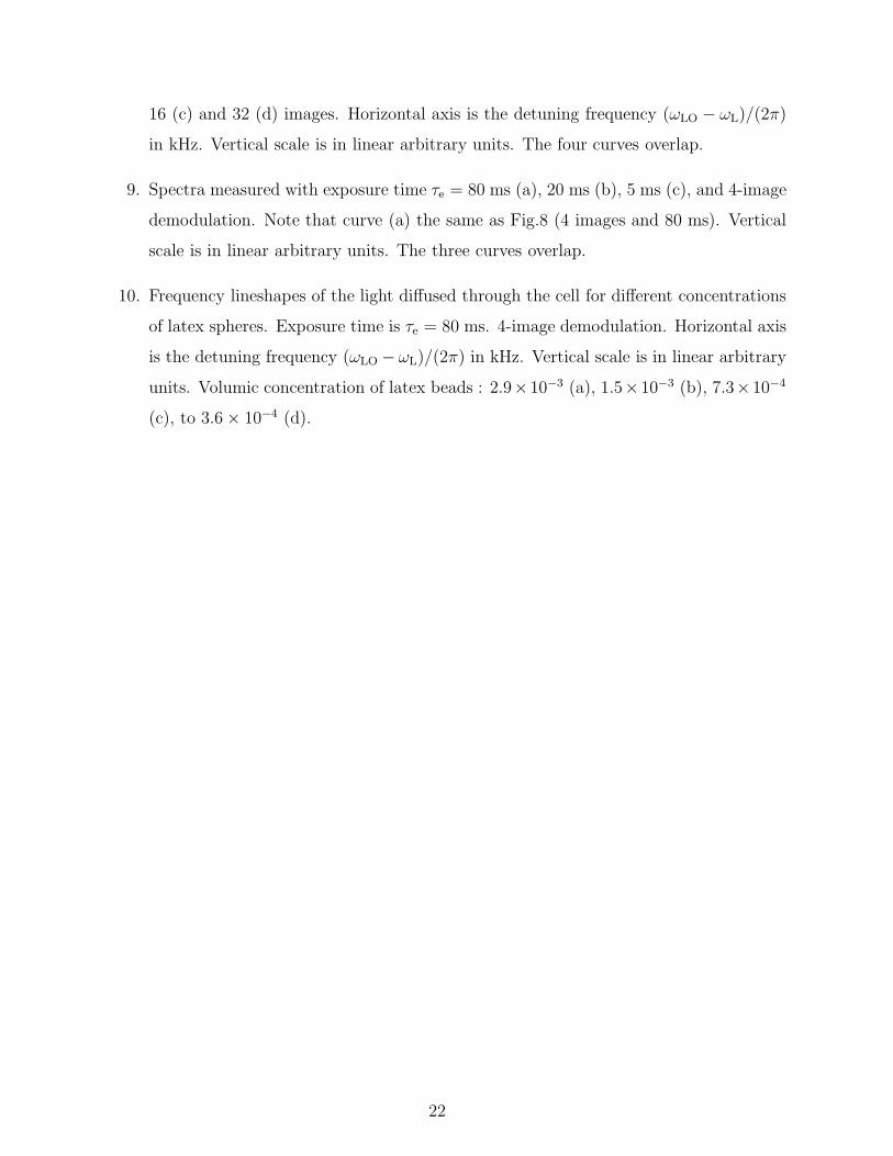
techniques [1]. They can be grouped in two categories [2, 3] : homodyne and heterodyne

schemes. In homodyne mixing (fig. 1(a)), self-beating object light impinges on a ∆ωPM-

bandwidth photodetector (also referred as optical mixer or photo-mixer, PM). To assess

a frequency component of the object light, the output of the PM is sent to a spectrum

analyser, whose bandwidth ∆ωF defines the detection resolution. The resulting spectra

are proportional to the second-order object field spectral distribution [2, 3] S2(ω). In

heterodyne mixing, sketched in fig. 1(b), the object light is mixed onto a PM with a

frequency-shifted reference beam, also called local oscillator (LO). The LO field (ELO) is

detuned to provoke a heterodyne beat of the object-LO field cross contributions to the

recorded intensity. This beat is sampled by a PM and sent to a spectrum analyser whose

bandwidth ∆ωF defines the apparatus resolution. This scheme enables one to measure the

first order object field spectral distribution S1(ω) [2, 3].

In heterodyne optical mixing experiments, the PM bandwidth ∆ωPM defines the span of

the measurable spectrum (usually ∼ 1 GHz). The resolution ∆ωF can be lowered down to

the sub Hertz range, which is suitable for, among other applications, spectroscopy of liquid

and solid surfaces [4], dynamic light scattering [2] and in vivo laser Doppler anemometry

[5]. But these schemes are inadequate for imaging applications, because measurements are

done on one point. The absence of spatial resolution has been sidestepped by scanning

techniques [6, 7], designed at the expense of temporal resolution.

2

We present a heterodyne optical mixing detection scheme on an array detector (configu-

ration of fig. 1(b)). Typical array detectors sampling rates seldom run over 1 kHz, failing

to provide a bandwidth large enough for most Doppler applications to date. Nevertheless,

their strong advantage is to perform a parallel detection over a large number of pixels. We

present a spatial and temporal modulation scheme (spatiotemporal heterodyning) that uses

the spatial sampling capabilities of an area detector to counterbalance the noise issue of a

measurement in heterodyne configuration performed in the low temporal frequency range

(e.g. with a typical CCD camera). The issue of using narrow-bandwidth camera PMs is

alleviated by detuning the LO field optical frequency accordingly to the desired spectral

point of the object field to measure. Post-detection filtering results from a numerical

Fourier transform over a limited number of acquired images.

This heterodyne optical mixing scheme on a low frame rate array detector can be used

as a filter to analyze coherent light. It has already been used in several applications yet,

including the detection of ultrasound-modulated diffuse photons [8, 9], low-light spectrum

analysis [10], laser Doppler imaging [11, 12, 13], and dynamic coherent backscattering effect

study [14]. The purpose of this paper is to present its mechanism.

Time domain description of the fields

We consider the spatially and temporally coherent light field of a CW, single axial mode

laser (dimensionless scalar representation) :

EL(t) = ALAt(t) exp (iωLt + iφ(t)) (1)

where ωL is the angular optical frequency, AL is the amplitude of the field (positive constant),

At(t) = 1 + a(t); |a(t)| ≪ 1 describes the laser amplitude fluctuations and φ(t) the phase

fluctuations. This field shines a collection of scatterers that re-emits the object field (or

scattered field), described by the following function :

EO(t) = AOXt(t)At(t) exp (iωLt + iφ(t)) (2)

where AO is a positive constant and Xt(t) is the time-domain phase and amplitude fluc-

tuation induced by dynamic scattering of the laser field, i.e. the cause of the object field

3

fluctuations due to dynamic scattering we intend to study. As in conventional heterodyne

detection schemes, a part of the laser field, taken-out from the main beam constitutes the

reference (LO) field :

ELO(t) = ALOAt(t) exp (iωLOt + iφ(t)) (3)

where ALO is a positive constant. The LO optical frequency is shifted with respect to the

main laser beam by ωLO − ωL to provoke a tunable temporal modulation of the interference

pattern resulting from the mix of the scattered and reference fields. It can be done

experimentally by diffracting the reference beam with RF-driven Bragg cells (acousto-optic

modulators) for example.

The expression of the light instant intensity impinging on the camera PMs is :

i(t) ≃ i0(Re[E])2 (4)

where i0 is a positive constant and Re[E] is the real part of the relevant optical complex field

E. The PMs are considered point-like, their antenna properties [15] are out of the scope of

this paper. To take into account the frequency filtering implication of finite time-domain

integration, the average intensity detected by the square-law camera PMs is :

I(t) = I0

∫ τe/2

−τe/2(E(t + τ) + E∗(t + τ))2 dτ (5)

where I0 is a positive constant and τe the exposure time. In the frequency-domain, this

integration corresponds to a sinc-shaped low-pass filter function whose bandwidth (defined

as the distance between the peak and the first zero) is 1/τe.

OPTICAL CONFIGURATION

Setup

The common name for optical mixing experiments on an array detector is digital

holography. The original underlying interference technique was invented to improve

electron microscopy resolution and was successfully applied to monochromatic light imaging

[16]. Since the availability of lasers and then digital cameras, digital holography [17] has

become an integrant part of many coherent imaging schemes, for its propensity to record

4

both quadratures of an optical field.

The optical configuration we use can be either a lensless Fourier off-axis holography setup

[18, 19] or a Fresnel off-axis holography setup [20]. In the lensless setup, sketched in fig. 2,

and considered throughout this study, the point source of the spherical reference wave (LO

focal point) is located at (x′

0, y′

0) in the plane of the object to match the average curvature

of the object field. An interference pattern is recorded in the camera plane (x, y). The

reconstruction algorithm used to calculate the spatial distribution of the scattered field in

the object plane consists of only one spatial fast Fourier transform (FFT) [19]. This setup

is used to avoid the need of a general Fresnel reconstruction algorithm. In the Fresnel setup

[20], the LO is a plane wave and the image reconstruction requires the use of numerical

lenses and at least two successive spatial domain FFTs [21].

The digital hologram is recorded with the frequency-shifting method introduced in the

heterodyne holography technique [22], used in several imaging and detection schemes [8, 9,

10, 12] for its ability to discriminate efficiently a few Doppler-shifted photons, according to

their frequency, from background light [8, 10]. The frequency-shifting method was chosen

as an accurate [22] dynamic phase-shifting detection scheme. This method is derived from

static phase-shifting interferometry [23] applied to phase-shifting holography [24]. It consists

of detuning the LO optical frequency with respect to the main laser beam, to provoke a time

domain modulation of the intensity pattern resulting from the cross contribution of object

and LO fields.

Spatial and temporal dependencies

Space (subscript s) and time (subscript t) dependencies of X and A are noted X(x, y, t) =

Xs(x, y) ·Xt(t), A(x, y, t) = As(x, y) ·At(t). Spatial frequencies (subscript sf) and temporal

frequencies (subscript f) reciprocal distributions form Fourier pairs with time domain and

spatial domain distributions. We have :

Yf(ω) =∫ T/2

−T/2Yt(t) exp(−iωt) dt (6)

and

Ysf(ξ, η) =∫ ∆x/2

−∆x/2

∫ ∆y/2

−∆y/2Ys(x, y)

5

× exp(−2iπ(xξ + yη)) dx dy (7)

where Y is the considered distribution, T is the measurement time, ∆x and ∆y are the

camera sensor widths.

In the lensless Fourier configuration, the LO wave curvature matches the average curva-

ture of the object field. Therefore, the heterodyne interference pattern on the detector is

formally equivalent [18] to the one that would impinge on the detector under Fraunhofer con-

ditions. Consequently, we can consider the (far field diffraction) equivalent situation where

the LO wave is a tilted plane wave in the detector plane and the object field distribution

is the Fourier transform of its spatial distribution in the object plane. The object and LO

complex optical fields take the following form:

EO(x, y, t) =

AOXs(x, y)As(x, y)

×Xt(t)At(t) exp (iωLt + iφ(t)) (8)

ELO(x, y, t) =

ALOAs(x, y) exp (2iπ(xξ0 + yη0))

×At(t) exp (iωLOt + iφ(t)) (9)

where ξ0 = x′

0/(λd) and η0 = y′

0/(λd). The tilt angle of the reference field leads to the phase

factor exp (2iπ(xξ0 + yη0)). The detected intensity is :

I(x, y, t) =

I0

∫ τe/2

−τe/2[EO(x, y, t + τ) + ELO(x, y, t + τ)

+E∗

O(x, y, t + τ) + E∗

LO(x, y, t + τ)]2 dτ (10)

Expression 10 has 16 terms among which 10 vanish because of the presence of optical fre-

quencies in the phase factors [4], which lead to oscillations outside the detection bandwidth.

It can be rewritten as :

I(x, y, t)/I0 =

AOALO I1(x, y) · I1(t)

6

+AOALO I2(x, y) · I2(t)

+A2LO I3(x, y) · I3(t)

+A2O I4(x, y) · I4(t) (11)

where the time-domain fluctuations of the intensity are :

I1(t) =∫ τe/2

−τe/2Xt(t + τ) |At(t + τ)|2

× exp (−i(ωLO − ωL)(t + τ)) dτ (12)

I2(t) =∫ τe/2

−τe/2X∗

t (t + τ) |At(t + τ)|2

× exp (i(ωLO − ωL)(t + τ)) dτ (13)

I3(t) =∫ τe/2

−τe/2|At(t + τ)|2 dτ (14)

I4(t) =∫ τe/2

−τe/2|Xt(t + τ)|2 |At(t + τ)|2 dτ (15)

and the spatial contributions to the intensity take the following form :

I1(x, y) =

|As(x, y)|2 Xs(x, y) exp (2iπ(xξ0 + yη0)) (16)

I2(x, y) =

|As(x, y)|2 X∗

s (x, y) exp (−2iπ(xξ0 + yη0)) (17)

where ξ0 = x′

0/(λd) and η0 = y′

0/(λd).

I3(x, y) = |As(x, y)|2 (18)

I4(x, y) = |Xs(x, y)|2 |As(x, y)|2 (19)

Temporal and spatial dependencies can be treated separately. Eq. 11 has four terms : the

first two are object-LO field cross terms. The third and fourth terms correspond to the LO

and object fields self beating contributions. The two first spatial contributions, I1(x, y) &

I2(x, y) will be referred as heterodyne, and I3(x, y) & I4(x, y) as homodyne, as well as their

7

temporal counterparts.

An assumption about the relative amplitudes of the fields is usually made [2] : the object

field amplitude is much lower than the LO field amplitude (heterodyne regime) :

AO ≪ ALO (20)

This assumption leads to neglecting the object field self-beating contribution, because its

relative amplitude with respect to the cross terms is AO/ALO ≪ 1. Additionally, in usual

optical mixing schemes on photodiodes, laser amplitude fluctuations are neglected (i.e.

a(t) = 0) [2, 4], since the measurement is done with detectors whose bandwidth is large

enough to make this assumption valid, as the detection is made at higher frequencies. But

with a slow PM such as a CCD camera, the frequency-domain noise resulting from these

fluctuations is not negligible.

A sequence of n images is sampled and leads to a data cube I(x, y, t), acquired for a given

detuning frequency ωLO − ωL. To make a spatial map of one frequency component of the

object field, a demodulation in the time and spatial domains is performed. As we will see,

the heterodyne holography scheme allows encoding of the spectral and spatial information

about the object field in the reciprocal space of the data cube, and it also allows spatial

discrimination of the self beating terms from the object-LO field cross terms.

SIGNAL DEMODULATION IN THE TIME DOMAIN.

I1 and I2 are referred as the heterodyne terms (modulated at the detuning frequency

ωLO − ωL, on purpose). They correspond to the object and LO field cross terms. I3

and I4 are referred as the homodyne terms (not explicitly modulated at the detuning

frequency). These terms correspond to the object field (and the LO field) self beating

intensity contributions.

To measure a spectral component of the object field, n samples of I(x, y, t) along the

time axis are acquired. These images are used to calculate both quadratures of the object

field by making a time domain demodulation consisting of calculating the first harmonic

8

component (I(x, y, ωS/n)) of the recorded sequence. This method is also used in temporal

heterodyne inline holography [25, 26]. The relation between the result of this demodulation

and the temporal frequency content of the object field is investigated.

First heterodyne term

Let’s consider the first heterodyne term :

I1(t) = F (t) exp(−i(ωLO − ωL)t) (21)

where F (t) is :

F (t) =∫ τe/2

−τe/2|At(t + τ)|2 Xt(t + τ)

× exp(−i(ωLO − ωL)τ) dτ (22)

According to eq. 22, F (t) corresponds to the result of the application of a bandpass filter

(of center frequency ωLO − ωL and bandwidth 1/τe) on Xt(t).

To demodulate the signal, the first harmonic (ωS/n) of the sampled image sequence is

calculated by FFT :

I1(ωS/n) =n

∑

k=1

I1(tk) exp(−2ikπ/n) (23)

where tk = 2kπ/ωS is the instant at which the kth image is recorded. We have :

I1(ωS/n) =n

∑

k=1

F (tk) exp(−i(ωLO − ωL)tk)

× exp(−2ikπ/n) (24)

I1(ωS/n) is a measurement of the ωLO −ωL + ωS/n frequency component of F (t) (the corre-

sponding instrumental bandwidth is ωS/n). Eq. 22 and 24 show that the spectral resolution

of this measurement should either be limited by the measurement time (n/ωS) and/or the

spectral distribution of the amplitude noise of the laser.

Second heterodyne term

The assessment of the quantity I2(ωS/n) is straightforward :

I2(ωS/n) =n

∑

k=1

F ∗(tk) exp(i(ωLO − ωL)tk)

9

× exp(−2ikπ/n) (25)

where F ∗(t) is the complex conjugate of F (t) defined by eq. 22. Equations 22 and 25 define

the action of two successive selective filters on Xt(t). The filters bandwidths are the same

as the ones introduced to describe the first heterodyne term. Their action is presented and

compared to their counterparts appearing in the first homodyne term in the next section.

Bandpass filtering

If we neglect the contribution of the amplitude fluctuations At(t) to the laser linewidth,

the impulse response functions for the first and second heterodyne terms (B+(ωLO − ωL)

and B−(ωLO − ωL) respectively) calculated by setting Xt(t) = 1 in expressions 24, 25 and

22 take the form :

B±(ωLO − ωL) = sinc ((ωLO − ωL) τe)

×n

∑

k=1

exp(−2ikπ/n) exp(∓2ikπωLO − ωL

ωS

) (26)

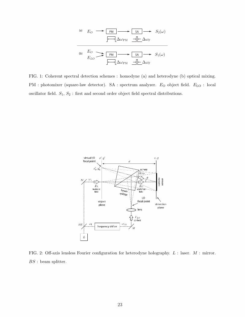
The instrumental response |B±(ωLO − ωL)|2 was measured experimentally, by analyzing

light backscattered by a static object. Data points of this instrumental response are

plotted as a function of the detuning frequency in fig. 3. The square amplitude of the

function described by eq. 26 is represented in fig. 4. Although their shape is similar, the

dynamic range of the theoretical filter is wider than the measured response. The difference

is attributed to the linewidth contribution of laser intensity fluctuations. One important

thing to remark about those instrumental responses is their dissymmetry.

|I1(ωS/n)|2 and |I2(ωS/n)|2 are calculated to represent quantities homogenous to the

optical power of the object field. This power is proportional to the object field power

resulting from the integration of its spectral density in the B± windows. We call these

distributions signal (or true image) and ghost (or twin image), respectively. B± describe

bandpass filters of width ∆ωF = ωS/n, centered on ωLO − ωL ± ωS/n. Consequently, this

scheme allows one to measure the ωLO − ωL ± ωS/n frequency components of the object

field fluctuations Xt(t).

10

If we set the detuning frequency to :

ωLO − ωL = ∆ω − ωS/n (27)

the signal will correspond to the ∆ω frequency component of the field and the ghost area

to the ∆ω + 2ωS/n component. We have |I1(ωS/n)|2 ≈ S1(∆ω) and |I2(ωS/n)|2 ≈ S1(∆ω +

2ωS/n). The corresponding frequency diagram is sketched in fig. 5.

Homodyne terms. LO and object fields self beating

In usual heterodyne monodetection schemes, self-beating contributions are considered as

an unavoidable noise component, which can actually be neglected in a high bandwidth PM

detection scheme. When using low frequency PMs such as camera pixels, these homodyne

contributions (defined by eqs. 14 and 15) have to be taken into account. We show in the

next section how these terms are filtered-out spatially in the detection process.

SIGNAL DEMODULATION IN THE SPATIAL DOMAIN. FILTERING OF SELF-

BEATING CONTRIBUTIONS

Heterodyne contributions

The precious advantage of holography is to allow sampling of the diffracted object

complex field (in phase and amplitude), whose spatial distribution in the detector plane is

described by the Xs(x, y) function. The time domain demodulation presented in the previous

section enables one to measure the spatial distribution of a tunable frequency component

of the object field, in amplitude and phase (i.e. both quadratures). Thus, after tem-

poral demodulation, the actual complex distributions defined by eqs. 16 and 17 are available.

As a result of the off-axis configuration, the object-LO field cross terms (or heterodyne

contributions) carry phase factors exp (±2iπ(xξ0 + yη0)). The relative distance between

each point (x′, y′) of the object (described by Xs(x′, y′)) and the LO focal point (x′

0, y′

0) in

the object plane is encoded in a set of parallel (complex) Young’s fringes in the detector

plane (x, y). The periods of these fringes are (λd/(x′ − x′

0) and λd/(y′ − y′

0)). Their spatial

11

frequencies are noted ∆ξ0 = (x′ − x′

0)/(λd) and ∆η0 = (y′ − y′

0)/(λd).

In Fraunhofer conditions, the relative distances between each point of the object (x′, y′)

and the LO focal point (x′

0, y′

0) are proportional to the spatial frequencies of the hologram

in the camera plane (ξ, η). We have :

|Xsf(ξ = x′/(λd), η = y′/(λd))|2∝ |Xs(x

′, y′)|2

(28)

Hence the requirement for only one spatial Fourier transform to reconstruct the image

[19, 21, 27] , i.e. to calculate the spatial distribution |Xs(x′, y′)|2.

The laser amplitude noise leads to flat-field fluctuations in the camera plane. The spatial

frequencies distribution of this noise is considered to be a centered dirac :

∫ ∆x/2

−∆x/2

∫ ∆y/2

−∆y/2|As(x, y)|2

× exp(

−2iπ

λd(xx′ + yy′)

)

dx dy

≈ δ(x′, y′) (29)

this assumption is implicit in lensless digital holography. The spatial frequency content of

I1(x, y) , assessed by a FFT, takes the following form :

|I1(ξ = x′/(λd), η = y′/(λd))|2∝

|Xs(x′ − x′

0, y′ − y′

0)|2

(30)

The ghost distribution is :

|I2(ξ = x′/(λd), η = y′/(λd))|2∝

|Xs(x′

0 − x′, y′

0 − y′)|2

(31)

In the lensless configuration, both signal and ghost spatial distributions are focused in the

same reconstruction plane. Eqs. 30 and 31 define two spatial distributions flipped one with

respect to the other and shifted away by ±(x′

0, y′

0) from the center of the reconstructed

hologram. The spatial instrumental response width corresponds to less than the distance

between two adjacent pixels in the reconstructed image [27]; its contribution is neglected.

12

Homodyne contributions

The object and LO self beating contributions I3 and I4 are not encoded in the spatial

complex fringe system which results from the interference of the object field and the off-

axis LO. Under the assumption of a perfect flat-field amplitude noise (eq. 29), the spatial

frequency content of eqs. 18 and 19 take the form :

I3(ξ = x′/(λd), η = y′/(λd)) ∝ δ(x′, y′) (32)

and

I4(ξ = x′/(λd), η = y′/(λd)) ∝

Xs(x′, y′) ∗ X∗

s (x′, y′) (33)

These terms are restituted inline : they are centered on (x′ = 0, y′ = 0) in the hologram

reconstructed in the object plane. This enables one to discriminate them spatially from

off-axis heterodyne contributions.

EXPERIMENTS

In previous publications [11, 12, 13], the spatiotemporal heterodyne detection technique

was used to perform parallel imaging. Here, we will focus our attention on the temporal

domain. We will study in particular how measured frequency spectra are affected by the

camera frame rate, exposure time, and total measurement time.

Setup and data acquisition details

The experimental setup, which is sketched in Fig.2, has been described previously [10,

11, 12, 13]. The light source is a Sanyo DL-7140-201 diode laser (λ = 780 nm, 50 mW

for 95 mA of current), the camera is a PCO Pixelfly digital CCD camera (12 bit, frame

rate ωS/(2π) ≃ 12.5 Hz, exposure time τe ≤ 2π/ωS = 80 ms, with 1280 × 1024 pixels of

6.7× 6.7 µm), and the frequency shifter is a set of two acousto-optic modulators AOM1 and

AOM2 (Crystal Technology; ωAOM1,2 ≃ 80 MHz). A neutral density is used to control the

LO beam intensity. The sample is a 1 cm × 1 cm × 5 cm rectangular PMMA transparent

cell filled with a diluted suspension of latex spheres in water (Polybead: Polyscience Inc.,

13

diameter 0.48 µm, undiluted concentration: 2.62% solids-latex). The Polybead suspension

is diluted by a factor ≃ 9 (0.5 ml of undiluted suspension + 4 ml of water). A rectangular

aperture (7 mm× 3 cm) located just in front of the cell removes the parasitic light diffused

along cell sides. The aperture delimiting the imaged side of the cell is located at a distance

d ≃ 39 cm of the camera. This sample is observed in transmission and the spectrum of

the light dynamically scattered by the latex spheres in brownian motion is measured by

sweeping the AOM1 frequency so that the detuning frequency ωLO − ωL is swept from 0

to 16 kHz in 81 frequency points (200 Hz step). For each frequency point a sequence of

32 consecutive CCD frames is recorded to the PC computer hard disk. For each frequency

sweep, 32 × 81 = 2592 images are recorded.

Data analysis

A first experiment consists of acquiring data with 3 frequency sweeps with τe = 80 ms,

τe = 20 ms and τe = 5 ms. For each frequency point, a n = 4 phase demodulation is

performed by using either 4, 8, 16 or the complete set of 32 recorded images. When more

than 4 images are used, a first n = 4 phase demodulation is done with images 1 to 4, which

is followed by a second demodulation with images 5 to 8, and so on. The complex signal

resulting from the demodulation of each set of 4 images is then summed to get the final

demodulation result. The total measurement time of one frequency point vary from 320 ms

(4 × 80 ms) to 2.6 s (32 × 80 ms), while the total exposure time vary from 20 ms (4 × τe

with τe = 5 ms) to 2.6 s (32 × τe with τe = 80 ms).

Fig. 6 represents the resulting images of the rectangular aperture, illuminated in

transmission via the diffusing cell, for an exposure time τe = 80 ms, and for a detuning

frequency (ωLO − ωL)/(2π) of 0 Hz (a), 400 Hz (b), 4000 Hz (c) and 8000 Hz (d). The

images are k-space images obtained by FFT of the hologram measured in the CCD plane

and n = 4 phase demodulation with 4 images per frequency point. They are displayed

in arbitrary logarithmic scale. The true image (signal) of the rectangular aperture is the

region 1 in fig. 6(a). This distribution is the spectral component of the object field of

frequency ωL −ωS/n. The twin image (ghost) of the aperture is the region 3. In accordance

with eq. 30 and 31, it is symmetric with respect to the center (tag 2) of the k-space plane

14

(null spatial frequency). The twin image corresponds to the ωL + ωS/n spectral component.

Increasing the detuning frequency ωLO − ωL, the true and twin images of the aperture

become darker and darker. Nevertheless, they are still visible for a 8000 Hz offset. One can

notice that for null detuning (fig. 6(a)) some statically scattered parasitic light is detected

out of the aperture image (region 4). This parasitic light is no more detected when the

frequency offset is non zero (images (b) to (d)).

To perform a quantitative analysis of the signal, we have summed the signal intensity

along the columns of the images represented on Fig.6, from line 312 to line 712 (horizontal

dashed lines on Fig.6(a)). These traces are represented on fig. 7. The true image corresponds

to region 1, the twin image to region 2. Regions 3 and 4 correspond to the background

signal. As mentioned in [8, 10], this background signal is due to the shot-noise on the LO.

Taking into account the heterodyne gain, the background signal corresponds to an optical

signal of one photo electron per pixel for the whole measurement sequence. The background

signal provides here a very simple absolute calibration for the optical signal diffused by the

sample. Here, in the center of the aperture, the sample diffused signal is about 3.5 times

the background i.e. 3.5 photo electron per pixel.

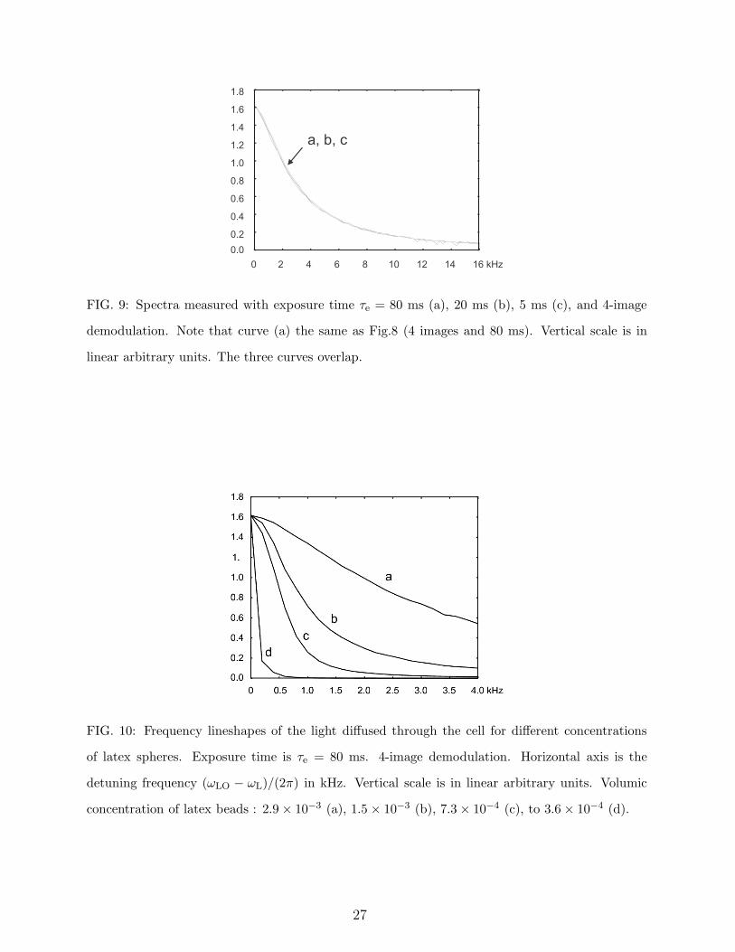
Spectra of Doppler-broadened light in the kHz range

From the reconstructed images (Fig.6), we have calculated the shape of the first order

spectrum of the diffused object field. To get these spectra, we have calculated the sum of

the area of the true image and twin image areas (regions 1 and 2 in the traces of fig. 7),

and subtracted the background (regions 3 and 4 in fig. 7). Fig. 8 and Fig. 9 show brownian

frequency spectra of the light dynamically scattered through the cell. These curves have

been normalized by the area under the raw lineshapes.

Data was collected for detuning frequencies up to 16 kHz, much larger than the hetero-

dyne receiver bandwidth (0.4 Hz for curve (d), reciprocal of the 2.6 s measurement time).

The shape of the spectrum does not depend on the number of images used to perform the

demodulation, as we can see in Fig. 8. In the range of exposure times τe (of one frame) used

for the measurement, the shape of the spectra reported on fig. 9 does vary with τe for the

15

following values of the latter : 5 ms (curve c), 20 ms (curve b), and 80 ms (curve a). Fig.8

and Fig.9, which exhibit the same lineshape, show that these spectra do not depend on the

total exposure time, which varies from 20 ms (Fig. 9(c)) to 2.6 s (Fig. 8(d)). One must

notice that these results are valid because the width of the spectrum (≃ 2.5 kHz half width)

is large compared to the instrumental response. In the all the presented results, the in-

strumental response is always smaller than 1/τe ≤ 200 Hz (width of the sinc factor in Eq.26).

Additionally, we measured the first order spectrum of the object field in fixed instrumental

conditions (4-phase demodulation, exposure time τe = 80 ms) to study different samples.

The scattering parameters of the suspension were changed in the following manner : the

latex beads concentration was halved from one measurement to another. The four Doppler

lineshapes reported on fig. 10 correspond to latex volumic fractions ranging from 2.9×10−3

(curve a) to 3.6 × 10−4 (curve d).

DISCUSSION

The presented technique uses and goes beyond the concept of time-average holography.

In time-averaged holography, the detector, whose exposure time τe is large, behaves as a

low-pass filter of bandwidth 1/τe. It selects the field components EO(ω) whose frequencies

ω = ωL +∆ω are close to ωLO, i.e. which satisfy |∆ω|τe < 1). This low-pass filtering effect is

used to study vibrating objects like musical instruments [28] by imaging the regions which

are not moving or which move with a given phase and velocity. In the first case (selection

of the non moving regions), the LO beam is not shifted in frequency [29, 30]. In the second

case (moving regions), the LO beam is modulated at the object vibration frequency [31, 32]

(which, in the temporal frequency domain, corresponds to the generation of adequate LO

frequency sidebands.

Our scheme enables detection of a tunable frequency component of the light with a sharp

bandwidth defined by the inverse of the acquisition time of a sequence of n images. But

reading-out an optical beat at typically low camera frame rates is difficult in practice in

the case of a weak-amplitude object field, because the low frequency part of the temporal

frequency spectrum is highly noisy : it contains LO and object field self-beating contribu-

16

tions. To discriminate the signal from these noise contributions, a lensless Fourier off-axis

configuration is used to encode, in a Young fringe system, the distribution of relative posi-

tions of object points with respect to the reference point. This scheme allows to restitute

the object field spatial distribution in the Fourier reciprocal space of the detection plane.

Having recourse to an off-axis configuration to sample the heterodyne optical beat enables

spatial frequency discrimination of the heterodyne terms (object and reference light cross

terms) carrying useful information from the object and reference light self-beating terms

carrying what turns out to be unwanted information. Time domain and spatial domain

modulation/demodulation schemes present strong similarities. Equation 16 is the spatial

counterpart of eq. 21. Signal and ghost distributions are beating at ±ωS/n in time domain.

This beating enables to perform a n-phase temporal demodulation of the recorded image

sequence to assess object and ghost fields in quadrature. Since these complex fields are

spatially modulated because of the off-axis interferometry configuration (according to eqs.

16 and 17), their distributions in the object plane are translated by ±(x′

0, y′

0) (respectively)

away from (0, 0)-centered homodyne contributions. This is highly valuable since it allows

one to filter them out spatially.

CONCLUSION

The presented scheme, based on heterodyne optical mixing onto a parallel detector used

as a selective frequency filter, is particulary suited to high resolution spectral imaging.

An tunable frequency component of the object field is acquired at a time. The camera

finite exposure time and the finite measurement time lead to a frequency domain bandpass

filter, which width is the reciprocal of the measurement time. The small dissymmetry of

the frequency domain instrumental response should be taken into account in quantitative

measurements. The available range of frequency shifts at which measurements can be

made is not limited to the photo-mixer bandwidth (contrary to wide-field laser Doppler

[33]), and benefits from heterodyne amplification. The measurement is sensitive : thanks

to the off-axis holographic setup, the self beating intensity contributions resulting from

laser instabilities and scattered light self interference within the camera bandwidth can

be efficiently filtered-out. The propensity to separate spatially cross terms intensity

contributions from self beating contributions lies in the use of a spatial heterodyne method.

17

The presented scheme is the association of a spatial and a temporal heterodyne detection.

Both temporal and spatial resolution are potentially high. This combination is enabled

by a wide field measurement performed at one frequency point at a time. The data transfer

rate bottleneck implies a tradeoff between the number of pixels in the image and the frame

rate of the detector, which should be guided by the application needs in terms of temporal,

spectral and spatial resolution. In a few words, combining a spatiotemporal modulation

and demodulation of a coherent probe light allows one to achieve a sensitive wide field

detection of a tunable Hertz-resolved spectral component with an array detector.

The authors acknowledge support from the French National Research Agency (ANR)

and from Paris VI University (BQR grant).

∗ Corresponding author: atlan@lkb.ens.fr

[1] A. T. Forrester. Photoelectric mixing as a spectroscopic tool. J. Opt. Soc. Am., 51:253, 1961.

[2] B. J. Berne and R. Pecora. Dynamic Light Scattering. Dover, 2000.

[3] Judith C. Brown. Optical correlations and spectra. American Journal of Physics, 51(11):1008–

1011, 1983.

[4] DS Chung, KY Lee, and E Mazur. Fourier-transform heterodyne spectroscopy of liquid and

solid surfaces. Applied physics. B, Lasers and optics, 64:1, 1997.

[5] MD Stern, DL Lappe, PD Bowen, JE Chimosky, GA Holloway, HR Keiser, and RL Bowman.

Continuous measurement of tissue blood flow by laser-doppler spectroscopy. American journal

of physiology, 232(4):H441, 1977.

[6] TJH Essex and PO Byrne. A laser doppler scanner for imaging blood flow in skin. J Biomed

Eng, 13(3):189, 1991.

[7] J. D. Briers. Laser doppler, speckle and related techniques for blood perfusion mapping and

imaging. Physiological Measurement, 22:R35–R66, 2001.

[8] M. Gross, P. Goy, and M. Al-Koussa. Shot-noise detection of ultrasound-tagged photons in

ultrasound-modulated optical imaging. Optics Letters, 28:2482–2484, 2003.

18

[9] M. Atlan, B.C. Forget, F. Ramaz, A.C. Boccara, and M. Gross. Pulsed acousto-optic imag-

ing in dynamic scattering media with heterodyne parallel speckle detection. Opt. Lett.,

30(11):1360–1362, 2005.

[10] M. Gross, P. Goy, B.C. Forget, M. Atlan, F. Ramaz, A.C. Boccara, and A.K. Dunn. Het-

erodyne detection of multiply scattered monochromatic light with a multipixel detector. Opt.

Lett., 30(11):1357–1359, 2005.

[11] M. Atlan and M. Gross. Laser doppler imaging, revisited. Review of Scientific Instruments,

77(11), 2006.

[12] M. Atlan, M. Gross, T. Vitalis, A. Rancillac, B. C. Forget, and A. K. Dunn. Frequency-

domain, wide-field laser doppler in vivo imaging. Optics Letters, 31(18), 2006.

[13] M. Atlan, M. Gross, and J. Leng. Laser doppler imaging of microflow. Journal of the European

Optical Society - Rapid publications, 1:06025–1, 2006.

[14] Max Lesaffre, Michael Atlan, and Michel Gross. Effect of the photon’s brownian doppler shift

on the weak-localization coherent-backscattering cone. Physical Review Letters, 97(3):033901,

2006.

[15] A.E. Siegman. The antenna properties of optical heterodyne receivers. Applied Optics,

5(10):1588, 1966.

[16] D. Gabor. A new microscopic principle. Nature, 161:777–778, 1948.

[17] J. W. Goodman and R. W. Lawrence. Digital image formation from electronically detected

holograms. Applied Physics Letters, 11(3):77–79, 1967.

[18] George W. Stroke. Lensless fourier-transform method for optical holography. Applied Physics

Letters, 6(10):201–203, 1965.

[19] Christoph Wagner, Sonke Seebacher, Wolfgang Osten, and Werner Juptner. Digital recording

and numerical reconstruction of lensless fourier holograms in optical metrology. Applied Optics,

38:4812–4820, 1999.

[20] U. Schnars. Direct phase determination in hologram interferometry with use of digitally

recorded holograms. Journal of Optical Society of America A., 11(7):2011, 1994.

[21] U. Schnars and W. P. O. Juptner. Digital recording and numerical reconstruction of holograms.

Meas. Sci. Technol., 13:R85–R101, 2002.

[22] F. LeClerc, L. Collot, and M. Gross. Numerical heterodyne holography with two-dimensional

photodetector arrays. Optics Letters, 25(10):716–718, 2000.

19

[23] Katherine Creath. Phase-shifting speckle interferometry. Applied Optics, 24(18):3053, 1985.

[24] I. Yamaguchi and T. Zhang. Phase-shifting digital holography. Optics Letters, 18:31, 1997.

[25] Guy Indebetouw and Prapong Klysubun. Space–time digital holography: A three-dimensional

microscopic imaging scheme with an arbitrary degree of spatial coherence. Applied Physics

Letters, 75(14):2017–2019, 1999.

[26] G. Indebetouw and P. Klysubun. Spatiotemporal digital microholography. Optical Society of

America Journal A, 18:319–325, February 2001.

[27] Thomas M. Kreis. Frequency analysis of digital holography. Optical Engineering, 41(4):771–

778, 2002.

[28] N. Demoli and I. Demoli. Dynamic modal characterization of musical instruments using digital

holography. Opt. Express, 13:4812–4817, 2005.

[29] Pascal Picart, Eric Moisson, and Denis Mounier. Twin-sensitivity measurement by spatial

multiplexing of digitally recorded holograms. Applied Optics, 42(11):1947–1957, 2003.

[30] R. L. Powell and K. A. Stetson. Interferometric vibration analysis by wavefront reconstruction.

J. Opt. Soc. Am., 55:1593, 1965.

[31] C. C. Aleksoff. Time average holography extended. Appl. Phys. Lett, 14:23, 1969.

[32] O. J. Lokberg. Espi- the ultimate holographic tool for vibration analysis. J. Acoust. Soc. Am.,

55:1783, 1984.

[33] A. Serov, B. Steinacher, and T. Lasser. Full-field laser doppler perfusion imaging monitoring

with an intelligent cmos camera. Opt. Ex., 13(10):3681, 2005.

20

LIST OF FIGURE CAPTIONS

1. Coherent spectral detection schemes : homodyne (a) and heterodyne (b) optical mix-

ing. PM : photomixer (square-law detector). SA : spectrum analyzer. EO object

field. ELO : local oscillator field. S1, S2 : first and second order object field spectral

distributions.

2. Off-axis lensless Fourier configuration for heterodyne holography. L : laser. M :

mirror. BS : beam splitter.

3. Measurement of the temporal frequency instrumental response. Camera framerate :

ωS/2π = 8 Hz. Exposure time : τe = 124 ms. n = 4. Representation of instrumental

responses for the true image (signal) and the twin image (ghost), in dB. Horizontal

axis : detuning frequency (ωLO − ωL)/(2π), in Hz. Squares : signal (first heterodyne

term). Circles : ghost (second heterodyne term).

4. Squared amplitude of the instrumental response defined by eq. 26. Camera fram-

erate : ωS/2π = 8 Hz. Exposure time : τe = 124 ms. n = 4. Representation of

10 log10[|B±(ωLO − ωL)|2], in dB. Horizontal axis : detuning frequency (ωLO−ωL)/(2π),

in Hz. Dotted line : B+. Continuous line : B−.

5. Frequency diagram of heterodyne terms spectral components in the case where the

detuning frequency is set to ωLO − ωL = ∆ω − ωS/n.

6. Images (1024× 1024 pixels) of the sample for (ωLO − ωL)/(2π) equal to 0 Hz (a), 400

Hz (b), 4000 Hz (c) and 8000 Hz (80 ms image exposure time, 4-image demodulation.

Arbitrary logarithmic scale display.

7. Traces obtained by summation along columns of Fig.6(a) to (d) intensities. Curves a

to d correspond to a detuning frequency (ωLO − ωL)/(2π) equal to 0 Hz (a), 400 Hz

(b), 4000 Hz (c) and 8000 Hz (d). Horizontal scale is the image horizontal pixel index.

Vertical scale is in linear arbitrary units.

8. Frequency spectra of the light diffused through a suspension of latex particles in brown-

ian motion. Exposure time is τe = 80 ms. Demodulation is performed with 4 (a), 8 (b),

21

16 (c) and 32 (d) images. Horizontal axis is the detuning frequency (ωLO − ωL)/(2π)

in kHz. Vertical scale is in linear arbitrary units. The four curves overlap.

9. Spectra measured with exposure time τe = 80 ms (a), 20 ms (b), 5 ms (c), and 4-image

demodulation. Note that curve (a) the same as Fig.8 (4 images and 80 ms). Vertical

scale is in linear arbitrary units. The three curves overlap.

10. Frequency lineshapes of the light diffused through the cell for different concentrations

of latex spheres. Exposure time is τe = 80 ms. 4-image demodulation. Horizontal axis

is the detuning frequency (ωLO − ωL)/(2π) in kHz. Vertical scale is in linear arbitrary

units. Volumic concentration of latex beads : 2.9×10−3 (a), 1.5×10−3 (b), 7.3×10−4

(c), to 3.6 × 10−4 (d).

22

PM

PM

SA

SA

EO

EO

ELO

(a)

(b)

S2(!)

S1(!)

É!F

É!F

É!PM

É!PM

FIG. 1: Coherent spectral detection schemes : homodyne (a) and heterodyne (b) optical mixing.

PM : photomixer (square-law detector). SA : spectrum analyzer. EO object field. ELO : local

oscillator field. S1, S2 : first and second order object field spectral distributions.

FIG. 2: Off-axis lensless Fourier configuration for heterodyne holography. L : laser. M : mirror.

BS : beam splitter.

23

-30 -20 -10 0 10 20 300

5

10

15

20

detuning frequency (Hz)

signal ghost

FIG. 3: Measurement of the temporal frequency instrumental response. Camera framerate :

ωS/2π = 8 Hz. Exposure time : τe = 124ms. n = 4. Representation of instrumental responses

for the true image (signal) and the twin image (ghost), in dB. Horizontal axis : detuning fre-

quency (ωLO − ωL)/(2π), in Hz. Squares : signal (first heterodyne term). Circles : ghost (second

heterodyne term).

-30 -20 -10 0 10 20 30-50

-40

-30

-20

-10

0

detuning frequency (Hz)

Bà(!LO à !L)B+(!LO à !L)

FIG. 4: Squared amplitude of the instrumental response defined by eq. 26. Camera framerate :

ωS/2π = 8 Hz. Exposure time : τe = 124ms. n = 4. Representation of 10 log10[|B±(ωLO − ωL)|2],

in dB. Horizontal axis : detuning frequency (ωLO−ωL)/(2π), in Hz. Dotted line : B+. Continuous

line : B−

24

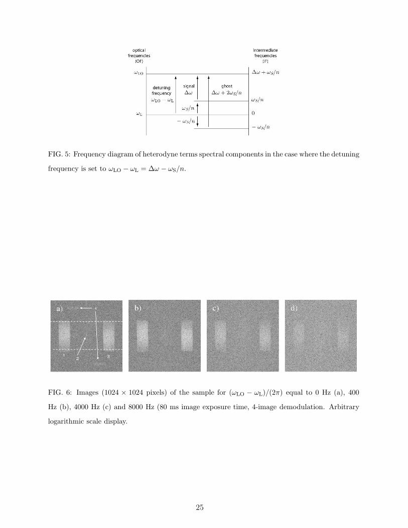
FIG. 5: Frequency diagram of heterodyne terms spectral components in the case where the detuning

frequency is set to ωLO − ωL = ∆ω − ωS/n.

FIG. 6: Images (1024 × 1024 pixels) of the sample for (ωLO − ωL)/(2π) equal to 0 Hz (a), 400

Hz (b), 4000 Hz (c) and 8000 Hz (80 ms image exposure time, 4-image demodulation. Arbitrary

logarithmic scale display.

25

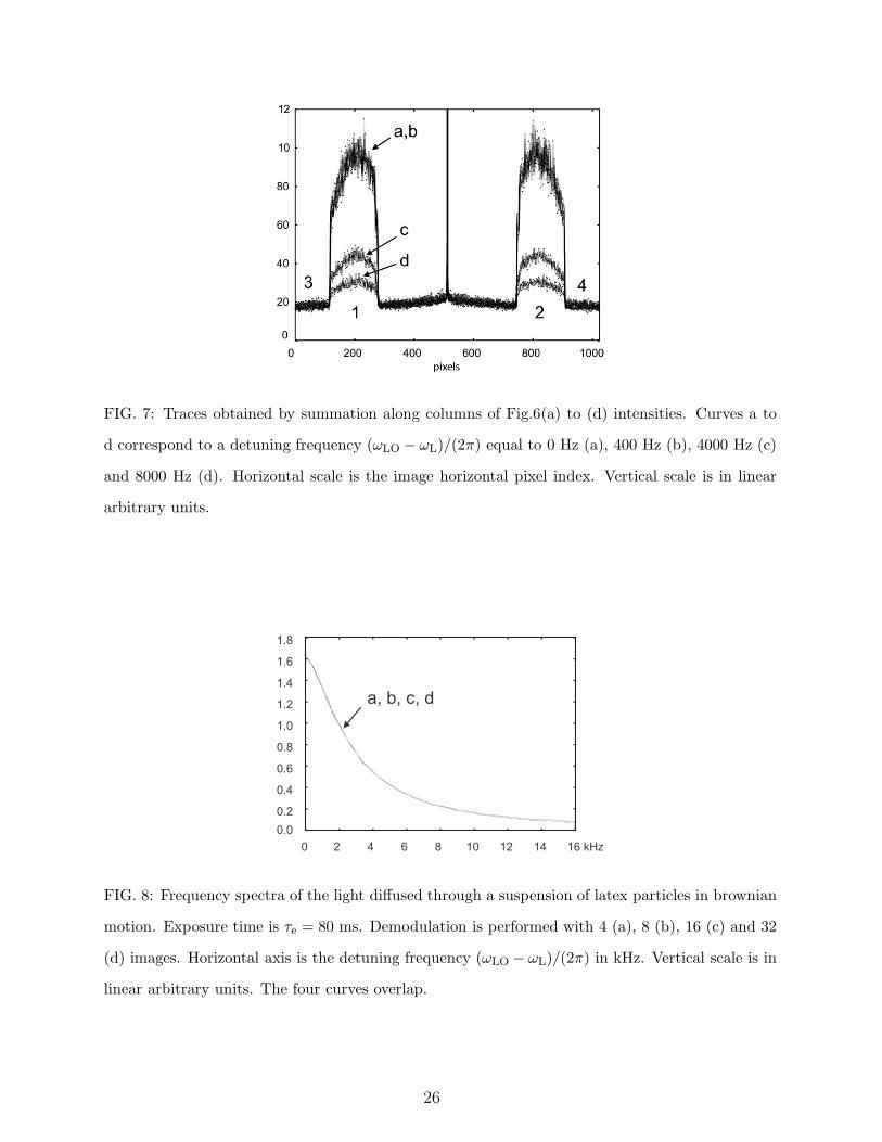
FIG. 7: Traces obtained by summation along columns of Fig.6(a) to (d) intensities. Curves a to

d correspond to a detuning frequency (ωLO − ωL)/(2π) equal to 0 Hz (a), 400 Hz (b), 4000 Hz (c)

and 8000 Hz (d). Horizontal scale is the image horizontal pixel index. Vertical scale is in linear

arbitrary units.

0.0

0.2

0.4

0.6

0.8

1.0

1.2

1.4

1.6

1.8

0 2 4 6 8 10 12 14 16 kHz

a, b, c, d

FIG. 8: Frequency spectra of the light diffused through a suspension of latex particles in brownian

motion. Exposure time is τe = 80 ms. Demodulation is performed with 4 (a), 8 (b), 16 (c) and 32

(d) images. Horizontal axis is the detuning frequency (ωLO − ωL)/(2π) in kHz. Vertical scale is in

linear arbitrary units. The four curves overlap.

26

0.0

0.2

0.4

0.6

0.8

1.0

1.2

1.4

1.6

1.8

a, b, c

0 2 4 6 8 10 12 14 16 kHz

FIG. 9: Spectra measured with exposure time τe = 80 ms (a), 20 ms (b), 5 ms (c), and 4-image

demodulation. Note that curve (a) the same as Fig.8 (4 images and 80 ms). Vertical scale is in

linear arbitrary units. The three curves overlap.

FIG. 10: Frequency lineshapes of the light diffused through the cell for different concentrations

of latex spheres. Exposure time is τe = 80 ms. 4-image demodulation. Horizontal axis is the

detuning frequency (ωLO − ωL)/(2π) in kHz. Vertical scale is in linear arbitrary units. Volumic

concentration of latex beads : 2.9 × 10−3 (a), 1.5 × 10−3 (b), 7.3 × 10−4 (c), to 3.6 × 10−4 (d).

27