
Visual transformation for interactive spatiotemporal data mining
Upload
khangminh22Category
view
4download
0
Doctoral Thesis in Computer Science
Learning Spatiotemporal Features in Low-Data and Fine-Grained Action Recognition with an Application to Equine Pain BehaviorSOFIA BROOMÉ
Stockholm, Sweden 2022
kth royal institute of technology
Learning Spatiotemporal Features in Low-Data and Fine-Grained Action Recognition with an Application to Equine Pain BehaviorSOFIA BROOMÉ
Doctoral Thesis in Computer ScienceKTH Royal Institute of TechnologyStockholm, Sweden 2022
Academic Dissertation which, with due permission of the KTH Royal Institute of Technology, is submitted for public defence for the Degree of Doctor of Philosophy on Friday the 2nd September 2022, at 10:00 a.m. in F3, Lindstedtsvägen 26, Stockholm

© Sofia Broomé ISBN 978-91-8040-295-8TRITA-EECS-AVL-2022:45 Printed by: Universitetsservice US-AB, Sweden 2022

i
Abstract
Recognition of pain in animals is important because pain compromisesanimal welfare and can be a manifestation of disease. This is a difficult taskfor veterinarians and caretakers, partly because horses, being prey animals,display subtle pain behavior, and because they cannot verbalize their pain.An automated video-based system has a large potential to improve the con-sistency and efficiency of pain predictions.
Video recording is desirable for ethological studies because it interferesminimally with the animal, in contrast to more invasive measurement tech-niques, such as accelerometers. Moreover, to be able to say something mean-ingful about animal behavior, the subject needs to be studied for longer thanthe exposure of single images. In deep learning, we have not come as far forvideo as we have for single images, and even more questions remain regardingwhat types of architectures should be used and what these models are actu-ally learning. Collecting video data with controlled moderate pain labels isboth laborious and involves real animals, and the amount of such data shouldtherefore be limited. The low-data scenario, in particular, is under-exploredin action recognition, in favor of the ongoing exploration of how well largemodels can learn large datasets.
The first theme of the thesis is automated recognition of equine pain. Here,we propose a method for end-to-end equine pain recognition from video, find-ing, in particular, that the temporal modeling ability of the artificial neuralnetwork is important to improve the classification. We surpass veterinarianexperts on a dataset with horses undergoing well-defined moderate experi-mental pain induction. Next, we investigate domain transfer to another typeof pain in horses: less defined, longer-acting and lower-grade orthopedic pain.We find that a smaller, recurrent video model is more robust to domain shifton a target dataset than a large, pre-trained, 3D CNN, having equal perfor-mance on a source dataset. We also discuss challenges with learning videofeatures on real-world datasets.
Motivated by questions arisen within the application area, the secondtheme of the thesis is empirical properties of deep video models. Here, westudy the spatiotemporal features that are learned by deep video models inend-to-end video classification and propose an explainability method as a toolfor such investigations. Further, the question of whether different approachesto frame dependency treatment in video models affect their cross-domaingeneralization ability is explored through empirical study. We also proposenew datasets for light-weight temporal modeling and to investigate texturebias within action recognition.
Keywords: Equine pain, computer vision for animals, deep learning, deepvideo models, spatiotemporal features, video understanding, action recognition,frame dependency, video data, end-to-end learning, temporal modeling

ii
Sammanfattning
Smartigenkanning hos djur ar viktigt for att smarta begransar djurs valfardoch kan vara ett sjukdomsuttryck. Att kanna igen smarta ar en svar upp-gift for veterinarer och djurskotare, delvis for att hastar, i egenskap av by-tesdjur, visar subtilt smartbeteende, och for att de inte kan verbalisera sinsmarta. Ett automatiserat videobaserat system har stor potential att forbattraoverensstammelsen och effektiviteten av smartdiagnostik.
Videoinspelning ar onskvart som datainsamlingsmetod for etologiska stu-dier for att det stor djuret minimalt, till skillnad fran mer invasiva teknikersasom rorelsesensorer. For att kunna saga nagot meningsfullt om djurbeteendebehover dessutom subjektet studeras langre an exponeringen for en stillbild.I djupinlarning har vi inte kommit lika langt for video som for stillbilder,och annu fler fragor aterstar angaende vilka arkitekturer som bor anvandasoch vad dessa modeller faktiskt lar sig. Att samla in videodata med kontrol-lerad och mattlig smartinduktion ar bade arbetsamt och involverar riktigadjur – mangden sadan data bor darfor vara begransad. Scenarier med be-gransad data ar under-utforskade inom videoklassificering, till forman for detbrett pagaende undersokandet av hur bra stora modeller kan lara sig storadatamangder.
Avhandlingens forsta tema ar automatiserad igenkanning av hastens smarta.Har foreslar vi en metod for smartigenkanning hos hastar, som opererarborjan-till-slut pa ra videodata, och finner specifikt att formagan att mo-dellera tidsdimensionen hos data for artificiella neurala natverk forbattrarderas smartigenkanningsformaga. Vi overtraffar veterinarexperter pa en da-tamangd med hastar som genomgar en valdefinierad mattlig experimentellsmartinduktion. Darefter undersoker vi domanoverforing till en annan smarttyphos hastar: mindre valdefinierad, langre verkande och mer laggradig ortope-disk smarta. Vi finner da att en mindre, rekurrent videomodell ar mer robustnar det kommer till domanskifte pa en maldatamangd an ett stort, fortranat3-dimensionellt faltningsnatverk, nar bada modeller har samma resultat pa enkalldatamangd. Vi diskuterar ocksa utmaningar med inlarning av videopre-diktorer pa datamangder inspelade for uppgifter i riktiga varlden (i motsatstill datamangder for konkurrensanalys inom maskininlarning).
Avhandlingens andra tema ar empiriska egenskaper hos djupa videomo-deller, motiverat av fragor som uppstatt i tillampningsomradet. Har studerarvi spatiotemporala prediktorer som ar inlarda av djupa videomodeller underborjan-till-slut-klassificering, och foreslar en forklaringsmetod som ett verk-tyg for dessa undersokningar. Vidare undersoks empiriskt fragan om huruvidaolika matematiska tillvagagangssatt for att behandla tidsberoendet mellan vi-deorutor paverkar deras kors-doman-generalisering. Vi presenterar ocksa nyadatamangder for lattviktig temporal modellering och for att kunna utreda fallav textursnedvridning inom videoklassificering.

List of Papers
The thesis is based on the following papers:
I Dynamics are Important for the Recognition of Equine Pain in VideoSofia Broome, Karina B. Gleerup, Pia H. Andersen, Hedvig KjellstromPublished in IEEE/CVF Conference on Computer Vision and Pattern Recog-nition (CVPR), 2019.
II Interpreting video features: a comparison of 3D convolutional net-works and convolutional LSTM networksJoonatan Manttari*, Sofia Broome*, John Folkesson, Hedvig KjellstromPublished in 15th Asian Conference on Computer Vision (ACCV), 2020.
III Sharing Pain: Using Pain Domain Transfer for Video Recognitionof Low Grade Orthopedic Pain in HorsesSofia Broome, Katrina Ask, Maheen Rashid, Pia H. Andersen,Hedvig KjellstromPublished in PLOS ONE, 2022.
IV Recur, Attend or Convolve? Frame Dependency Modeling Mattersfor Cross-Domain Robustness in Action RecognitionSofia Broome, Ernest Pokropek, Boyu Li, Hedvig KjellstromUnder review, 2022.
Other contributions by the author not included in the thesis:
V Improving gait classification in horses by using inertial measure-ment unit (IMU) generated data and machine learningF.M. Serra Braganca, Sofia Broome, M. Rhodin, S. Bjornsdottir, V. Gun-narsson, J.P. Voskamp, E. Persson-Sjodin, W. Back, G. Lindgren, M. Novoa-Bravo, A.I. Gmel, C. Roepstorff, B.J. van der Zwaag, P.R. Van Weeren, E.HernlundPublished in Nature Scientific reports, 2020.
* Authors contributed equally.
iii

iv LIST OF PAPERS
VI Towards Machine Recognition of Facial Expressions of Pain in HorsesPia H. Andersen, Sofia Broome, Maheen Rashid, Johan Lundblad, KatrinaAsk, Zhenghong Li, Elin Hernlund, Marie Rhodin, Hedvig KjellstromPublished in Animals, 2021.
VII Equine Pain Behavior Classification via Self-Supervised Disentan-gled Pose RepresentationMaheen Rashid, Sofia Broome, Katrina Ask, Pia Haubro Andersen, HedvigKjellstromPublished in IEEE Winter Conference on Applications of Computer Vision(WACV), 2022.
VIII Going Deeper than Tracking: a Survey of Computer-Vision BasedRecognition of Animal Pain and Affective StatesSofia Broome*, Marcelo Feighelstein*, Anna Zamansky*, Gabriel Lencioni*,Pia Haubro Andersen, Francisca Pessanha, Marwa Mahmoud, Hedvig Kjell-strom, Albert Ali SalahUnder review, 2022.

Acknowledgements
It goes without saying that many people have supported, inspired or taughtme things during these years. First of all, Hedvig, filing under all of those three:thank you for believing in me and giving me the chance to be your student.You have granted me large freedom, encouraged my ideas and more importantlyhelped me sharpen them. Your knowledge and experience in computer visionhave always guided me in understanding what is important, as well as helpedme grasp the field and its development. Thank you also for your kindness andunderstanding when life has had its ups and downs.
My co-supervisor Pia Haubro Andersen has tirelessly explained and sharedher knowledge of physiology, pain, and behavior of horses with me and providedimportant guidance on how to think about this research problem. More broadly,I am grateful to all of the researchers from SLU involved in and surrounding theequine pain recognition project: Pia Haubro Andersen, Elin Hernlund, KarinaBech Gleerup, Marie Rhodin and Katrina Ask. From when I first met (most of)you, on the trip to northern California in May 2017 where we filmed horses, a fewmonths before my Ph.D. officially started, and through the years of collaborating,you have been living examples for me of how to conduct focused and meaningfulwork, and all the while enjoying it. You were always smart, kind and open, andresearch seemed like the most natural thing for you, which was vital for me tojust observe. There was also always something beautiful to me about the forcerequired in your clinical work, how to keep a horse’s lungs from collapsing underthe animal’s weight during surgery, or how to remove the eye of a cow standingout on a field.
I also want to thank Maheen Rashid-Engstrom for being who you are andfor appearing in my life as a kind of elder sister in computer vision research,demystifying the creation of a paper (by making it look easy, from running ofexperiments to writing) – I learned so much from you, while at the same timebeing a friend that I could talk about anything with, and for our collaborationon the WACV paper.
I will always be grateful to Martin Hwasser who gave me confidence in pro-gramming around the time between my bachelor’s and master’s, basically taughtme Git and Vim and importantly how to set the keyboard to U.S. keys and makethe terminal look nice. Without you in my life during those years I would not
v

vi ACKNOWLEDGEMENTS
have dared to choose the machine learning master’s program, which led to thisthesis. And thank you for still being a friend, whether in machine learning ordancehall.
Next, I want to thank RPL which has been a wonderful lab to be part of.I am grateful to the teachers in the AI course round of 2015, in particular toPatric Jensfelt, Akshaya Thippur and Judith Butepage who gave me the chanceto become a teaching assistant in the course during my master’s, which was myfirst encounter with RPL and eventually how I understood that I wanted toapply for a Ph.D. here. Later, when I was in the doctoral student union, I hadweekly meetings with the heads of RPL, Patric Jensfelt and Christian Smith,which I learned a lot from and where I always felt welcome, thank you both forthat. Josephine Sullivan, for being a great supervisor for my master’s thesis, andencouraging me to do research. You have been a mentor to me since then, guidingme many times, not least with great comments on the CVPR paper. Thank youto my friends in Hedvig’s group: Marcus Klasson, for many laughs and listeningto Bear Quartet in the office, Ruibo Tu, for often widening my perspective, TarasKucherenko, for being so honest and direct, Ci Li, for being the sweetest officeroommate and Olga Mikheeva, for your healthy skepticism toward deep learning.We have developed together and I have learned a lot from all of you. JoonatanManttari, for the good times and fluent collaboration when working on our ACCVpaper together. Ioanna Mitsioni, with whom I share a love for (and maybe exiledreams to) language. Irmak Dogan, with whom I share a fate of dislocatedjoints. Federico Baldassarre, for great discussions on deep learning and for videoin particular. Rika Antonova, Ylva Jansson and Hossein Azizpour for being rolemodels in intellectual curiosity. RPL has grown a lot these years and there aretoo many of us now to mention all, but I want to thank Alexis Linard, Alex Sleat,Atsuto Maki, Christopher Sprague, Ciwan Ceylan, Daniel Sabel, Diogo Almeida,Ignacio Torroba, Iolanda Leite, Jana Tumova, Jesper Karlsson, Ludvig Ericsson,Matteo Gamba, Miquel Marti, Marten Bjorkman, Petter Ogren, Pouria Tajvar,Sanne van Waveren, Sarah Gillet, Sebastian Bujwid, Sebastian Gerard, VladislavPolianskii, Wenjie Yin and Yi Yang for being such kind and open persons.
However absurd and/or pretentious it is to feel inclined to summarize all partsof life on the occasion of writing a computer science thesis, the truth is that thechances in life are so few to put thankfulness in physical print. Therefore, herecomes more.
Thank you to my mother Marie-Louise for your love and support. Thank youto my father Michael, for insisting whenever I have been anxious about work thatunproductive hours are unavoidable in research and will eventually lead some-where, and that it is pointless to judge myself for it, this made a big difference.You are of course also the reason why I became fascinated with mathematics andscience to begin with; an early memory of you showing me how to program andvisualize the Mandelbrot set, because it is beautiful, comes to mind. Thank youto my grandmother Anne for also helping me to stress less and for our many longconversations about life. Thank you to my brother for being a brilliant person.

vii
We will be here until you get well, and after.Anna Torok, for being family. Tania Neuman, for saving me both in spring
2012 and spring 2019. Evelina Linnros, for explaining how the world works. Youhave all three been there more than half of my life now. Very unclear who I wouldhave been without growing up alongside you, which process is still ongoing, andwhich, if I’m lucky, will keep on. Anna Kulin, don’t know where to begin. Iremember celebrating that I had gotten the Ph.D. position in your old apartmentin Bagarmossen, I think you were the first I told. Miriam Lindal, for all thenights (years) finding and playing very rare rap songs together, to audiences bothgrateful and not. Josephine Schneider, for your presence and clear-sightednessin pretty much all areas of life. Sara Hansson Maleki, for sharing endorphins onthe way back from dance every week and very nerdy talking of specific dancehallgun steps, you’ve been a big source of happiness for me this spring while writing.Pella Myrstener, for teaching me about art history and for general therapy overthe years. Fanny Wallberg and Adrian Radway for understanding everything.Thank you all for your brilliance and love and for accepting me with my faults.Thank you, DJGC.
Sofia BroomeStockholm, June 2022


Acronyms
List of commonly used acronyms:
AU Action Unit (part of a FACS)C3D Convolutional 3D (Type of CNN)ConvLSTM Convolutional LSTMConvLSTM-2 Convolutional LSTM in two streams of RGB and optical flowCNN Convolutional Neural NetworkEOP(j) EquineOrthoPain(joint) (name of a dataset)EPS Equine Pain ScaleFACS Facial Action Coding Systemfps frames per secondGPU Graphics Processing UnitGRU Gated Recurrent UnitHOG Histogram of Oriented GradientsHGS Horse Grimace ScaleI3D Inflated 3D (Type of CNN)IEEE Institute of Electrical and Electronics EngineersLPS LipopolysaccharideLSTM Long Short-Term MemoryMIL Multiple-Instance LearningPF Pain Face (name of a dataset)ReLU Rectified Linear UnitRNN Recurrent Neural NetworkRGB Red Green Blue (color model)SVM Support Vector MachineTRN Temporal Relational NetworkTSN Temporal Segment NetworkTV Total VariationWSAR Weakly Supervised Action RecognitionWSAL Weakly Supervised Action Localization
ix


Contents
List of Papers iii
Acknowledgements v
Acronyms ix
Contents 1
1 Introduction 31.1 Contributions . . . . . . . . . . . . . . . . . . . . . . . . . . . . . . . 51.2 Thesis outline . . . . . . . . . . . . . . . . . . . . . . . . . . . . . . . 10
2 Background 132.1 Equine pain . . . . . . . . . . . . . . . . . . . . . . . . . . . . . . . . 132.2 Related work in automated pain recognition . . . . . . . . . . . . . . 192.3 Related work in action recognition . . . . . . . . . . . . . . . . . . . 282.4 Architectures . . . . . . . . . . . . . . . . . . . . . . . . . . . . . . . 36
3 Equine pain recognition 393.1 Datasets . . . . . . . . . . . . . . . . . . . . . . . . . . . . . . . . . . 393.2 Automated recognition of equine pain in video . . . . . . . . . . . . 443.3 Pain domain transfer . . . . . . . . . . . . . . . . . . . . . . . . . . . 583.4 Conclusions . . . . . . . . . . . . . . . . . . . . . . . . . . . . . . . . 76
4 Learning spatiotemporal features 774.1 Temporality is important for vision – yet it is under-used . . . . . . 784.2 Frame dependency treatment . . . . . . . . . . . . . . . . . . . . . . 804.3 The case for recurrence . . . . . . . . . . . . . . . . . . . . . . . . . 884.4 Conclusions . . . . . . . . . . . . . . . . . . . . . . . . . . . . . . . . 91
5 Empirical properties of deep video models 935.1 Datasets . . . . . . . . . . . . . . . . . . . . . . . . . . . . . . . . . . 935.2 Explaining video features . . . . . . . . . . . . . . . . . . . . . . . . 98
1

2 CONTENTS
5.3 Frame dependency modeling matters for cross-domain robustness inaction recognition . . . . . . . . . . . . . . . . . . . . . . . . . . . . . 114
5.4 Conclusions . . . . . . . . . . . . . . . . . . . . . . . . . . . . . . . . 129
6 Conclusions 1316.1 Summary . . . . . . . . . . . . . . . . . . . . . . . . . . . . . . . . . 1326.2 Limitations and future outlook . . . . . . . . . . . . . . . . . . . . . 133
References 135

Chapter 1
Introduction
This thesis concerns how deep learning methodology can be used to recognizeaspects of the internal state of an animal that cannot describe it in words tous. This requires following the animal over time, how it shifts from momentto moment, in facial expression or in pose. There is information lying in thetemporal dependency between visual snapshots of the animal, in how it movesits head from an upright position to somewhere else, or in how something brieflyflinches in its facial muscles, only for it to return to a relaxed gaze. Therefore,the temporal aspect is important for the application. In this work, specifically,the task has been to recognize the pain expressions of horses.
There are multiple layers of challenges when it comes to recognizing pain inhorses. First of all, we have not come as far in deep learning methods for videoas we have for single images. While the performance of artificial neural net-works (hereon, neural networks for brevity) on certain static image classificationtasks has surpassed human performance [1], the recognition of action classes fromdifferent viewpoints and with large variations in background clutter, which areeasily separable for humans, still lags behind. As an example of this, the bestperforming approach [2] on the HMDB dataset [3] with 51 classes (such as kiss,drink, run or push-up), achieves only 88% accuracy, whereas the current bestperforming approach [4] on ImageNet [5] with 1000 static classes achieves above90% accuracy. Second, this tasks contains the additional difficulty of not onlyrecognizing whether someone is, e.g., jumping or not, but also inferring the un-derlying emotion of that action or outward behavior. Third, there is controversyregarding the nature of pain. There is a difference between nociception, whichis the sensory nervous system’s response to harmful stimuli, and our actual sub-jective experience of pain. Humans have grimaces that we can make to expresspain, which occur already for infants. For horses and other mammal species aswell, facial expressions have been identified that are associated with pain. Butneither for humans nor for other animals is there a single known physiological orbiochemical parameter that says that pain is present without a doubt. Further-
3
4 CHAPTER 1. INTRODUCTION
more, horses have only 15 facial muscles [6], whereas humans have more than 40,which makes their faces less expressive than ours. This offers an argument tomake use of the temporal dimension when studying equine facial behavior. Last,horses are prey animals and tend to hide their pain, because they prefer not todisplay vulnerability.
The field of machine learning applied to image data has been transformed inthe past decade, through the use of deep learning [7]. Owing to the creation andavailability of large-scale labeled datasets, the facilitation of computation on GPUcards, such methods are now widely used in contexts outside of academia, e.g., inmobile phone applications or in software for self-driving cars. Given enough data,a neural network can be trained to recognize and distinguish visual patterns thatare pertinent to different semantic categories.
This development has enabled the study of animal behavior in ways thathave never been possible before, allowing for meticulous computer scanning andmodeling from visual recordings, which can be fine-grained both in space andtime. In fact, the field of computer vision for animals is attracting growinginterest, notably with the 2021 creation of a recurring workshop dedicated to thistheme at the world’s largest computer vision conference (IEEE/CVF Conferenceon Computer Vision and Pattern Recognition).
When it comes to motion and learning spatiotemporal features from animalbehavior or from video in general, deep learning is, as stated above, not as devel-oped as for single image analysis. It is difficult for a neural network to learn torecognize motion ‘templates’ and their semantics across varying appearances andbackgrounds [8], due to the sequentiality of the problem, which not only addsa dimension to an already high-dimensional sensory domain (vision) but also anew layer of abstraction – time. An introduced temporal dimension is vitallydifferent from a spatial one. What the concept of time entails may arguably notbe trivial to learn from scratch. Despite there being a large body of work onaction recognition, many deep video models still mainly learn to rely on spatialbackground cues [9, 10], when the task really should be about a pertinent objector agent moving in some or other space-time shape.
Recognition of pain in animals is important because pain compromises ani-mal welfare and can be a manifestation of disease. Pain diagnostics for humanstypically include self-evaluation with the help of standardized forms and label-ing of the pain by a clinical expert using pain scales, which naturally is difficultfor non-verbal species. Further, attempting to recognize pain in non-human ani-mals is inherently subjective and time consuming [11], and is therefore currentlychallenging for both horse owners and equine veterinarian experts.
Pain in horses is typically assessed by manually observing a combination ofbehavioral traits such as exploratory behavior, restlessness, positioning in the boxand changes in facial expressions [6]. Video filming can be used to prolong theobservation periods and increase the likelihood of capturing pain behavior, butit can take two hours to evaluate a two minute video clip using proper manualannotation, such as EquiFACS [6] for facial expressions, or for other behavioral

1.1. CONTRIBUTIONS 5
signs of pain. This severely limits the possibilities for routine pain diagnostics onhorses, for instance before or after surgery.
An accurate automatic pain detection method therefore has large potentialto increase animal welfare. Such a system would allow veterinarians and horseowners to reliably and frequently screen the pain level of the horses, and possiblyhelp unveil which behaviors are most likely associated with a painful experience.
1.1 Contributions
The furthering of machine learning methods for increased understanding of animalbehavior hinges on the ability of computer systems to extract relevant informa-tion from video data. Therefore, this thesis makes contributions in two machinelearning areas, which also constitute the two major themes of the thesis: auto-mated recognition of equine pain (the application area), and studies of empiricalproperties of deep video models, i.e., neural networks which learn features fromimage data with a temporal extent.
In the applied contribution of the thesis, we are the first to perform automaticpain recognition in horses. We are also the first to perform automatic pain recog-nition on video for any non-human species, as well as making the argument thatthis is important.
As for the part of the thesis treating deep video models, we contribute a uniquediscussion on the topic of learning spatiotemporal features outside of the cleanbench-marking realm in action recognition. We present results from experimentscomparing video models that are similar in that they learn spatial and temporalfeatures simultaneously, but differ principally in their mathematical approach tomodeling frame dependency. Since this has largely not been done previously,this has required devising new metrics and study designs that can capture rele-vant aspects of the features learned by these different types of models. We alsocontribute a new explainability method, as well as new datasets to investigatecross-domain robustness and background (texture) bias in action recognition.
Figure 1.1 shows a scheme of the four articles which lay the ground for thisthesis, and how they build on each other. In the first work, we find that pain recog-nition performance improves when using deep learning models with increased ca-pabilities of modeling the temporal dimension of the data. This result, togetherwith the fact that deep video models are typically even more obscure, i.e., largerin terms of trainable parameters, than single image models, led to the secondwork where we investigate explainability for video models, which was very unex-plored at the time. An explainability method is proposed for action recognition,and we conduct an empirical study based on the proposed method and other met-rics, to see whether models with different kinds of temporal dependency modelinglearn different kinds of features. Here, we compare 3D CNNs and ConvLSTMnetworks.

6 CHAPTER 1. INTRODUCTION
Figure 1.1: Overview and chronology of articles which lay the foundation of thethesis. The symbols at the top corner of each box indicate whether the article treatsequine pain or empirical properties of video models.
In the third work, I received a new equine pain dataset which contained record-ings based on a new type of pain induction (orthopedic pain, via a model for lame-ness). The labels of the dataset, as well as the ‘pain signal’, were significantlynoisier and weaker than in the first work. This eventually led us to investigatedomain transfer between the cleaner pain domain from the first work and thenoisier orthopedic pain domain. When comparing different types of models, wesaw indications that a 3D CNN had poorer generalization capabilities than asmaller recurrent (ConvLSTM) model.
This was the motivation for the fourth article, where we come back to thetheme of comparing video models with principally different mathematical modelsof time, to see whether this has implications for the type of spatiotemporal fea-tures that they learn. In this work, it is specifically the capacity for cross-domainrobustness that is investigated.
Parts of the thesis’ contents have been published previously in scientific arti-cles. Below, I list the four articles which the thesis is based on, in chronologicalorder, where in the thesis their contents are reflected, and the author contribu-tions for each one.
I Dynamics are Important for the Recognition of Equine Pain in VideoSofia Broome, Karina B. Gleerup, Pia H. Andersen, Hedvig Kjellstrom

1.1. CONTRIBUTIONS 7
Published in IEEE Conference on Computer Vision and Pattern Recognition(CVPR), 2019.
Abstract
A prerequisite to successfully alleviate pain in animals is to recognize it, whichis a great challenge in non-verbal species. Furthermore, prey animals such ashorses tend to hide their pain. In this study, we propose a deep recurrenttwo-stream architecture for the task of distinguishing pain from non-pain invideos of horses. Different models are evaluated on a unique dataset showinghorses under controlled trials with moderate pain induction, which has beenpresented in earlier work. Sequential models are experimentally comparedto single-frame models, showing the importance of the temporal dimensionof the data, and are benchmarked against a veterinary expert classificationof the data. We additionally perform baseline comparisons with generalizedversions of state-of-the-art human pain recognition methods. While equine paindetection in machine learning is a novel field, our results surpass veterinaryexpert performance and outperform pain detection results reported for otherlarger non-human species.
Part of the thesis
This work is mainly presented in Chapter 3 on equine pain recognition, Section3.2. Parts of its dataset descriptions appear in Section 3.1, and parts of itsrelated work appear in Section 2.3.
Author contributions
S.B. carried out the experiments and their analysis which led to the conceptof the article, wrote the manuscript, and coordinated the work on the paper.K.B.G. and P.H.A. provided data for the experiments from a previous study,provided supervision of S.B. in the application domain, and contributed to theequine pain sections of the manuscript. K.B.G. and P.H.A. also were helpful insetting up the human expert baseline study, otherwise mainly organized anddesigned by S.B. Data analysis of the human expert study was carried out byS.B. H.K. contributed with continuous supervision of S.B., ideas for experi-ments, and manuscript editing.
II Interpreting video features: a comparison of 3D convolutional net-works and convolutional LSTM networksJoonatan Manttari*, Sofia Broome*, John Folkesson, Hedvig KjellstromPublished in 15th Asian Conference on Computer Vision (ACCV), 2020.
Abstract
A number of techniques for interpretability have been presented for deep learn-ing in computer vision, typically with the goal of understanding what the net-works have based their classification on. However, interpretability for deepvideo architectures is still in its infancy and we do not yet have a clear concept

8 CHAPTER 1. INTRODUCTION
of how to decode spatiotemporal features. In this paper, we present a studycomparing how 3D convolutional networks and convolutional LSTM networkslearn features across temporally dependent frames. This is the first comparisonof two video models that both convolve to learn spatial features but have princi-pally different methods of modeling time. Additionally, we extend the conceptof meaningful perturbation introduced by [12] to the temporal dimension, toidentify the temporal part of a sequence most meaningful to the network for aclassification decision. Our findings indicate that the 3D convolutional modelconcentrates on shorter events in the input sequence, and places its spatialfocus on fewer, contiguous areas.
Part of the thesis
This work is mainly presented in Chapter 5, under Section 5.2. Parts of itsdataset descriptions are found in Section 5.1 and parts of its related work arefound in Section 2.3.
Author contributions
Experiments and first draft preparation were equally shared between S.B. andJ.M. S.B. conceptualized the empirical comparison between a ConvLSTM andof a 3D CNN, whereas J.M. proposed the Temporal Masks algorithm. S.B.implemented the project in Tensorflow, whereas J.M. implemented the projectin Pytorch. J.F. and H.K. provided continuous supervision of the two firstauthors, and contributed to the manuscript editing.
III Sharing Pain: Using Pain Domain Transfer for Video Recognitionof Low Grade Orthopedic Pain in HorsesSofia Broome, Katrina Ask, Maheen Rashid, Pia H. Andersen,Hedvig KjellstromPublished in PLoS ONE, 2022.
Abstract
Orthopedic disorders are common among horses, often leading to euthanasia,which often could have been avoided with earlier detection. These conditionsoften create varying degrees of subtle long-term pain. It is challenging to traina visual pain recognition method with video data depicting such pain, sincethe resulting pain behavior also is subtle, sparsely appearing, and varying,making it challenging for even an expert human labeller to provide accurateground-truth for the data. We show that a model trained solely on a datasetof horses with acute experimental pain (where labeling is less ambiguous) canaid recognition of the more subtle displays of orthopedic pain. Moreover,we present a human expert baseline for the problem, as well as an extensiveempirical study of various domain transfer methods and of what is detectedby the pain recognition method trained on clean experimental pain in theorthopedic dataset. Finally, this is accompanied with a discussion around the

1.1. CONTRIBUTIONS 9
challenges posed by real-world animal behavior datasets and how best practicescan be established for similar fine-grained action recognition tasks.
Part of the thesis
This work is mainly presented in Chapter 3, Section 3.3, on domain transferwithin equine pain recognition. Parts of its dataset descriptions are found inSection 3.1 and parts of its descriptions of equine pain appear in Section 2.1.
Author contributions
S.B. designed and carried out the experiments and their analysis which led tothe concept of the article, wrote the original draft and organized the work.K.A. and P.H.A. contributed to the manuscript parts regarding equine pain,further conceptualization regarding the pain domains, and also contributed tosetting up the interface for the human expert explainability study. The videodata used for training and evaluation were previously collected by K.A. andP.H.A. and others, as reported in earlier publications. M.R. contributed to themanuscript and in conceptualizing discussions with S.B. H.K. provided contin-uous supervision of S.B., ideas for experiments, as well as contributed to themanuscript writing.
IV Recur, Attend or Convolve? Frame Dependency Modeling Mattersfor Cross-Domain Robustness in Action RecognitionSofia Broome, Ernest Pokropek, Boyu Li, Hedvig KjellstromUnder review, 2022.
Abstract
Most action recognition models today are highly parameterized, and evaluatedon datasets with predominantly spatially distinct classes. Previous resultsfor single images have shown that 2D Convolutional Neural Networks (CNNs)tend to be biased toward texture rather than shape for various computer visiontasks [13], reducing generalization. Taken together, this raises suspicion thatlarge video models learn spurious correlations rather than to track relevantshapes over time and infer generalizable semantics from their movement. Anatural way to avoid parameter explosion when learning visual patterns overtime is to make use of recurrence across the time-axis. In this article, we em-pirically study the cross-domain robustness for recurrent, attention-based andconvolutional video models, respectively, to investigate whether this robustnessis influenced by the frame dependency modeling. Our novel Temporal Shapedataset is proposed as a light-weight dataset to assess the ability to generalizeacross temporal shapes which are not revealed from single frames. We find thatwhen controlling for performance and layer structure, recurrent models showbetter out-of-domain generalization ability on the Temporal Shape datasetthan convolution- and attention-based models. Moreover, our experiments in-dicate that convolution- and attention-based models exhibit more texture biason Diving48 than recurrent models.

10 CHAPTER 1. INTRODUCTION
Part of the thesis
This work is mainly presented in Chapter 5, Section 5.3. Descriptions of thedataset contributions appear in Section 5.1. Parts of its introduction appearin Section 4.3 and parts of its related work appear in Section 2.3.
Author contributions
S.B. formulated the research question and idea, designed all and conductedmost experiments and their analysis, wrote the manuscript and organized thework. E.P. conducted experiments involving the TimeSformer model and con-tributed to the original draft of the manuscript. B.L. formulated the textureconcept for a video setting (masking or cropping boxes of the agent in the clips),conducted a pilot study (MSc thesis supervised by S.B.), and contributed toediting of the final manuscript. H.K. provided continuous supervision of thefirst author, ideas for experiments, as well as contributed to the manuscriptwriting.
1.2 Thesis outline
This thesis is organized as follows. The first part of Chapter 2 presents relevantbackground for the equine pain application – general background on animal pain,equine pain and its assessment, current equine health in Sweden and distinctionsbetween different types of equine pain (Section 2.1). In the second and thirdsections of Chapter 2, related work within automatic pain recognition as well asaction recognition are presented. At the end of this chapter, some neural networkarchitectures that will occur throughout the thesis are introduced.
In Chapter 3, I present our applied work on automatic equine pain recognition.The chapter has two main parts, one about learning pain features end-to-end fromraw video data, and one part about how to move between different pain domains(from experimental acute pain to orthopedic pain).
Chapter 4 constitutes a bridge between the two themes of the thesis (equinepain and deep video models), and a preliminary to as well as a contextualizationof the experiments of Chapter 5. Conclusions and questions that arose fromthe results in Chapter 3 are discussed in the light of deep learning for video. Idiscuss why temporality is important in computer vision and then present anddiscuss the conceptual differences between three principally different approachesto frame dependency treatment when learning spatiotemporal features from videodata. Temporality in biological vision is further discussed.
In Chapter 5, I present results in the second major theme: empirical propertiesof deep video models. First, a method for explaining the decisions of such modelsis presented, followed by the measurement of several empirical properties of avariety of these models, including the capacity for generalization across domainshift.

1.2. THESIS OUTLINE 11
Last, I discuss and summarize the thesis findings in Chapter 6 with an outlookon possible future directions.
The online Appendix can be visited at https://sofiabroome.github.io/appendix.


Chapter 2
Background
To familiarize the reader with the application area, the first part of this chapterwill treat some essentials of equine pain (Section 2.1). The presentation will befar from exhaustive on the topic, and interested readers are asked to follow thereferences of the section. After this, I will survey the related work done thus farwithin computer vision-based pain recognition, with an emphasis on non-humanspecies, as well as more generally within action recognition (Section 2.3). Last,in Section 2.4, I introduce a group of neural network models that will appear inthe thesis.
2.1 Equine pain
Pain in animals, and in horses
Assessing pain in animals is a complex task. The International Association for theStudy of Pain (IASP) defines pain as ”an unpleasant sensory and emotional ex-perience associated with actual or potential tissue damage, or described in termsof such damage” [14]. For an event to count as painful, it should thus containboth potential tissue damage and a (to some extent) anguished experience. Whiletesting for nociception can be carried out in a rather straight-forward manner [15](by, e.g., measuring nociceptor firing), assessing pain requires assessing the sub-jective experience or internal state of another individual. This is difficult even forhumans, let alone for another species. It can be noted that as late as the 1980s,it was widely assumed that neonates did not experience pain as we do, togetherwith a hesitancy to administrate opiates to these patients, and surgery was oftenperformed without anaesthesia [16].
However, current evidence amounts beyond a reasonable doubt to the conclu-sion that both vertebrates and even certain invertebrates can experience pain [15].Furthermore, in the same way that we can never be sure that other animals doexperience pain, we cannot fully prove that they in fact do not experience pain.
13

14 CHAPTER 2. BACKGROUND
This warrants a precautionary principle in standards for handling, e.g., laboratoryanimals [17].
The evidence has been established based on a range of criteria. The animalshould have nociceptive receptors, i.e., receptors that respond to harmful stimuli,some central processing structure analogous to a cerebral cortex, and a connectionbetween the latter and the nociceptive receptors, in which nervous system opioidreceptors as well as internal opioid substances can be found. Furthermore, theanimal should adapt its behavior to avoid the cause of the pain when possible,beyond the initial reflex to avoid it, which does not require central processing.Upon receiving analgesics or pain relief in any form, the visible assumed painbehavior should be reduced. This is the case for most mammals, including horses.In the review by Sneddon et al., the definition of animal pain is extended toinclude a change in motivation, where the animal develops longer-term behaviorsto avoid pain or to protect the painful area. [15]
Depending on the origin of pain, the animal may perform different behaviors.In the case of horses, if they suffer from, e.g., visceral pain they may stretch, rolland kick toward the painful abdominal area, while horses with orthopedic painin the limbs may be reluctant to move and have an abnormal weight distributionor movement pattern [18]. Therefore, pain assessment tools such as pain scalesoften target pain of a specific origin.
Facial expressions, on the other hand, seem to be universal for pain withina species, first observed for humans [19]. In horses, this has been inferred fromthe fact that grimace scales have been successfully applied to pain from differentorigins, for example post-surgical pain and laminitis in horses [20–22]. It is alsosuspected that pain-related facial expressions are present during both acute andchronic pain. In rodents, painful grimacing has been recorded during severalweeks post-injury, but not necessarily consistently and perhaps tailing away [23].Systematic studies on facial expressions related to chronic pain have not beenconducted yet for horses. However, despite the difference in scale between horsesand rodents, the nervous system is similar across mammals, and thus one canpotentially expect analogous behavior in horses and other mammals.
It is important to study and learn to recognize pain to ensure the welfare ofnon-verbal species, for the large number of situations when this falls under ourresponsibility, legally or ethically [15]. Specifically, reducing pain to a minimumfor horses is shown to improve convalescence and optimize treatment success[24]. Pain detection and quantification in horses depend on an observer to detectpotentially pain related changes in behavior and in physiological parameters,which we will expand on next.
Pain assessment in horses
My work is motivated by the fact that it is difficult to evaluate pain in horses,and by the assumption that the practice of equine pain recognition currently issub-optimal. Human experts have low inter-rater agreement when assessing the

2.1. EQUINE PAIN 15
pain level in horses. As an example of this, veterinarians can score assumed painin horses associated with a particular condition on a range from ‘non-painful’ to‘very painful’ [25]. Such discrepancies can be particularly noticeable for low-gradepain [26–28]. The lack of consensus is troubling since veterinary decision-makingregarding pain recognition is critical for the care of animals in terms of prescribingalleviating treatments and in animal welfare assessments [29].
Nevertheless, within the last two decades, pain assessment in horses has drawnincreasing attention, in research as well as in clinical practice. This is bothbecause there is an increasing knowledge about the detrimental effects of painand because advanced treatments and surgical procedures have become morecommon for horses [30]. In other words, even if it is a difficult feat, the stateof pain equine recognition is perhaps better than ever, not least because it ismore acknowledged as important than ever. Yet, this should not be taken tomean that there is not a long road ahead. Compared to small animals, horsesare often not given the optimal pain treatment [31], and a study from the UKin 2005 showed that only 37% of veterinarians routinely administered analgesiaafter castration [32].
Within the growing study on equine pain, there is increasing focus on behav-ioral observations, since physiological parameters are often not pain-specific [33].Further, using behavioral observations as a proxy for pain is practical becausethese are both much less invasive and less cumbersome than measuring physio-logical parameters, nociceptive firing or so-called evoked response tests (whereinone sets up an experiment to measure the time it takes for an animal to withdrawthe painful body part in controlled settings [34]). Naturally, the latter is also lesspractical for large animals, compared to for rodents.
It has been found that horses’ behavioral activity time budget changes whenthey experience pain [35, 36]. This term refers to the fraction of their time thatthey spend, e.g., lying down, eating or being attentive. Records of similar activi-ties are part of certain composite pain scales, for example the Equine Pain Scale(EPS), proposed in the review by Gleerup and Lindegaard [30]. Also in the re-view, some general pain behaviors that have been observed in the veterinary painresearch literature are listed as reduced physical and social activity, less foraging,a lowered head, and standing further back inside the box.
Facial expressions is another behavioral category that has become more andmore commonly discussed and used in pain evaluation contexts in general. Thisdevelopment started with research on human pain, for non-verbal patients suchas neonates using the Facial Action Coding System developed by Ekman andFriesen [37]. It has now spread to multiple non-human species, such as cats,seals, pigs, dogs and rodents. So-called grimace scales or ‘pain faces’ have beendeveloped for at least ten species, and it has been hypothesized that the facialexpression may specifically signal the affective component of a pain event [23].Horses are one of these species, and equine facial expressions have lately beenpresented as a sensitive measure of pain, when observed in combination withother pain behaviors [21,30,38,39]. In the pain cases of the study by Dalla Costa
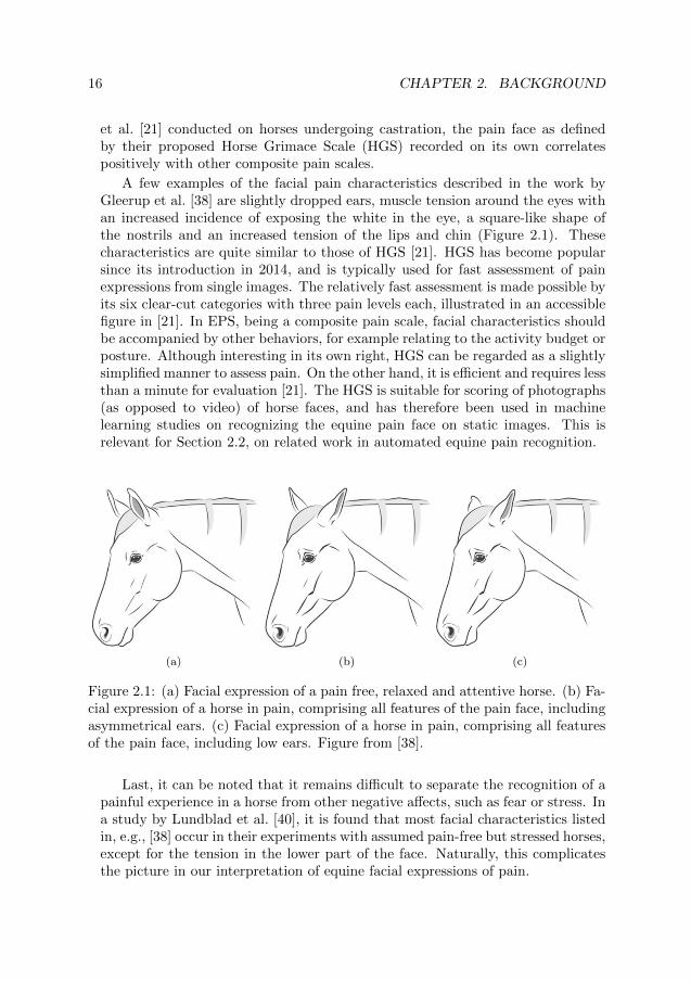
16 CHAPTER 2. BACKGROUND
et al. [21] conducted on horses undergoing castration, the pain face as definedby their proposed Horse Grimace Scale (HGS) recorded on its own correlatespositively with other composite pain scales.
A few examples of the facial pain characteristics described in the work byGleerup et al. [38] are slightly dropped ears, muscle tension around the eyes withan increased incidence of exposing the white in the eye, a square-like shape ofthe nostrils and an increased tension of the lips and chin (Figure 2.1). Thesecharacteristics are quite similar to those of HGS [21]. HGS has become popularsince its introduction in 2014, and is typically used for fast assessment of painexpressions from single images. The relatively fast assessment is made possible byits six clear-cut categories with three pain levels each, illustrated in an accessiblefigure in [21]. In EPS, being a composite pain scale, facial characteristics shouldbe accompanied by other behaviors, for example relating to the activity budget orposture. Although interesting in its own right, HGS can be regarded as a slightlysimplified manner to assess pain. On the other hand, it is efficient and requires lessthan a minute for evaluation [21]. The HGS is suitable for scoring of photographs(as opposed to video) of horse faces, and has therefore been used in machinelearning studies on recognizing the equine pain face on static images. This isrelevant for Section 2.2, on related work in automated equine pain recognition.
(a) (b) (c)
Figure 2.1: (a) Facial expression of a pain free, relaxed and attentive horse. (b) Fa-cial expression of a horse in pain, comprising all features of the pain face, includingasymmetrical ears. (c) Facial expression of a horse in pain, comprising all featuresof the pain face, including low ears. Figure from [38].
Last, it can be noted that it remains difficult to separate the recognition of apainful experience in a horse from other negative affects, such as fear or stress. Ina study by Lundblad et al. [40], it is found that most facial characteristics listedin, e.g., [38] occur in their experiments with assumed pain-free but stressed horses,except for the tension in the lower part of the face. Naturally, this complicatesthe picture in our interpretation of equine facial expressions of pain.

2.1. EQUINE PAIN 17
Different types of pain in horses
In any animal, one typically distinguishes between acute and chronic pain experi-ences. They are different in that the latter may be modulated over time by variousfactors, which can, e.g., make the pain sensation less localized to the initial causethan the acute pain. Acute pain has a sudden onset and a distinct cause, such asinflammation, while chronic pain is more complex, sometimes without a distinctcause, and by definition lasts for more than three months. Acute (and sometimeschronic) pain typically arises from the process of encoding an actually or poten-tially tissue-damaging event, so-called nociception, and may therefore be referredto as nociceptive pain. When pain is associated to decreased blood supply andtissue hypoxia, it is instead termed ischemic pain [41,42]. However, the characterof ischemic pain is acute, in that it has a fast onset and also recedes readily oncethe blood supply is released. Ischemic pain is thus a subset of acute pain. Inour work, we study acute pain, the main reason for which being that it would beeven more difficult to obtain labeled data for chronic pain. Studying acute painlets us work with more controlled experimental data and is a first step toward amore general pain recognition.
Orthopedic pain in horses can be of both acute and chronic character, althoughchronic states are suspected to be very common when it comes to the limbs. Onefrequent orthopedic diagnosis is osteoarthritis, or degenerative joint disease [43],with related inflammatory pain of the affected joint [44]. In humans, the diseaseis known to initially result in nociceptive pain localized to the affected joint, butwhen chronic pain develops, central sensitization occurs with a more widespreadpain [45]. How pain-related facial expressions and other behaviors vary betweenhorses with acute and chronic orthopedic pain is yet to be described, and so is therelation between pain intensity and alterations in facial expressions. In Section3.3, we investigate transfer learning between acute experimental nociceptive andischemic pain behavior and the more diffuse orthopedic pain behavior.
Different experimental pain models
In biology, a pain model is a means to study ongoing pain. It can either bea specific method to induce pain experimentally, or a specific choice of animalsto observe, for example horses post surgery, or horses that are suspected to bein pain for other reasons. Different pain models may be more or less clinicallyrelevant. Depending on the experimental setup, they also vary in how cleanlythe assumed painful sensation can be separated from other expected sensationsat the time for the experiment or observation.
The work presented in Chapter 3 uses datasets with recordings from threedifferent pain models, which will be further detailed in Section 3.1. The first twoare experimental moderately noxious stimuli which previously have been usedin human pain research [38]: capsaicin extract applied to the skin, and a bloodpressure cuff applied to one limb, creating ischemic pain. Both models create

18 CHAPTER 2. BACKGROUND
acute moderate pain, which appears and then recedes during a short period oftime. The third pain model is an injection of lipopolysaccharides (LPS) into ajoint, inducing inflammatory arthritis, which creates mild orthopedic pain. Theorthopedic pain in this model is technically acute, but its low-grade character andprogressing involvement of many different tissues of the joint makes it differentand more difficult to detect than the capsaicin and blood pressure cuff models.
Equine health in Sweden
What is, then, the current health situation of horses in Sweden? A large-scalestudy based on insurance data from 1997-2000 in Sweden was performed in 2005by Penell et al. [46]. The sample in the study constituted of approximately 75,000horses that were fully insured, which is estimated to have comprised around 34%of the Swedish horse population at the time. The yearly incidence out of 10,000‘horse years at risk’, i.e., the number of insurance claims per 10,000 insured horsesper year, was around 1100, or around 8000 among the total population of >70kinsured horses. Major causes for disease during these years were conditions in thelimbs and joints (for example arthritis and laminitis), colic (a sign of abdominalpain), and traumatic injuries to the skin [47]. More recent numbers from aninsurance company in 2021 show that orthopedic disorders make up around 50%of the morbidity among their insured horses [48]. More recent studies furtherpoint to many cases of undetected orthopedic pain in the horse population [49].Lameness is a sign of orthopedic disease that is difficult for humans to perceive[50, 51]. Therefore, orthopedic disease risks not being detected until signs aremore overt and the disease has progressed to stages which are more difficult totreat. Observing motion asymmetry is sensitive but not specific for lamenessdiagnostics. This underlines the importance of automated methods for detectingpain cues, in combination with motion measurements.
What can we gain from an automatic equine pain recognitionsystem?
Documenting both general behaviors and facial expressions in horses is very timeconsuming. Even though short, applicable pain scoring tools have been devel-oped [30], these do not capture all pain behavior but rather do spot sampling ofpre-determined behaviors that are suspected of being characteristic for the actualpain. One important advantage of an automatic pain recognition system wouldbe its ability to store information over time, and produce reliable predictions ac-cording to what has been learned previously. Humans are not able to remembermore than a few cues at the time when performing pain assessment. This high-lights the need for automated methods and prolonged observation periods, whereautomated recognition can indicate possible pain episodes for further scrutiny. Inequine veterinarian clinics, such a system would be of great value. Even a systemwith a less-than-perfect accuracy would be useful in conjunction with experts on

2.2. RELATED WORK IN AUTOMATED PAIN RECOGNITION 19
site. An automated means to record pain behavior from surveillance videos wouldbe an important step forward in equine pain research.
2.2 Related work in automated pain recognition
Below, I will go over the work that has been published so far within automatedpain recognition for non-human species. As preliminary matters, there is first anote on deep learning for readers approaching the topic from, e.g., an ethologyperspective, followed by a very brief overview of the field of automated painrecognition in humans. The latter is kept short both because this has alreadybeen covered in a number of review articles [52–55], but also because the problemhas slightly different challenges compared to the non-human case.
A general note on deep learning for interdisciplinary readers. Deeplearning is a methodology that is distinct from traditional machine learning andcomputer vision approaches in that the feature extraction from a certain data-point is learned, as opposed to being hand-crafted or pre-defined. In practice,this means that some number (for computer vision applications, typically in themillions range) of learnable parameters within a neural network are adapted to adataset throughout a number of training iterations on a particular task (e.g., clas-sification). The iterations are guided by the gradient (a generalized derivative)of a loss function (measuring the current performance on the task of the neuralnetwork), which points toward areas where the loss function has lower values (i.e.,lower error, which is desirable). This process is called gradient descent.
The parameters of a full deep learning pipeline can thus be trained end-to-end(from input to output), meaning that both the feature extraction layers and thetask-specific output layer (e.g., a classifier) are trained all at once. Dependingon the amount and types of labels that are accessible for a given dataset, thetraining scheme can be adopted to various levels of supervision. Recently, it iscommon to train the feature extraction part of a neural network using so-calledpretext tasks, whose labels arise automatically from the definition of the tasks(e.g., classification of the rotation that a natural image has undergone) – makingthe tasks self-supervised, rather than requiring the manual labelling of a fullysupervised scenario. This thesis, on the other hand, mainly investigates standardsupervised learning, although in challenging scenarios of low amounts of data,particularly in Chapter 3.
Automated pain recognition in humans
The field of automated pain recognition in humans is vast compared to for non-human species. The number of articles on the topic is in the hundreds [55],whereas for non-human species, it is around ten, at the time of writing this thesis(Table 2.1). The most notable difference between automated pain recognition in

20 CHAPTER 2. BACKGROUND
humans and other animals lies in the possibility to rely on self-report for groundtruth. Although such accounts unavoidably are subjective to their nature, theydo come at least closer to the internal experience of the subject than without averbal account.
A second important difference is the better opportunities for recording datawith consenting subjects that can sit still and be recorded in controlled settings.In this way, multi-modal databases such as the BioVid Heat Pain Database [56],BP4D+ [57], SenseEmotion [58], and EmoPain [59] have been possible to create.On the other hand, there are humans in pain that are non-verbal, which are lessrepresented in similar databases, such as persons afflicted with dementia, underanaesthesia, or otherwise with impaired speech. Typically, adult subjects in thementioned datasets are relatively young and healthy [55]. There is, however, onelarge non-verbal group which is represented in databases specific to their group:neonates. A survey specifically covering the work on neonate pain recognition isby Zamzmi et al. [52].
The main modalities that appear in similar databases are RGB footage (fo-cused on facial expressions, although body movement is present in a few), audio(vocalization), and time series of physiological parameters such as heart rate, skinconductance or electroencephalogram (EEG). Typical means of pain induction areheat or cold, for adults. For neonates, one common pain indicator is the drawingof blood samples from their heels (heel lancing). This permits to record expectedpain expressions without inducing pain that is not medically called for. [52, 55]
Overall, the trend, as in most machine learning applications, in this fieldis to move increasingly toward deep learning, with promising results. Notably,Rodriguez et al. [60] achieved more than 90% accuracy using deep learning onvideo on a binary pain recognition task of should pain in humans – the UNBC-McMaster Shoulder Pain Expression Archive Database [61]. The architecture wasa VGG-16 [62] pre-trained on the VGG Faces dataset [63], with an LSTM layerstacked on top for the temporal modeling. The dataset used in the article consistsof videos of humans self-identifying as having shoulder problems when performingdifferent range of motion tests. It can be noted that the labels are set from expertscoring of the pain expressions, rather than using baseline subjects performingthe same movement under no pain, presumably since there was a large variety inthe pain level of the different subjects. This question of labels based on expertsrather than on controlled pain experiments is discussed in the non-human contextfurther below.
Even though early (and non-deep learning) work by Littlewort et al. [64, 65]reports that a classifier can distinguish between genuine and posed pain expres-sions in humans, addressing the subjective experiential aspect and expression ofpain will remain a difficult or impossible aspect of any pain recognition approach,regardless of the species. This difficulty is also related to individual variability inpain expressions and general motivation to display pain or not. Nevertheless, thetechnology is well-developed for humans to recognize both faces and facial land-marks in order to extract specific action units, and even for detailed 3D modeling

2.2. RELATED WORK IN AUTOMATED PAIN RECOGNITION 21
of the human face [66], which is promising for systematic research on the facialpain expressions of humans. Furthermore, given that human faces are more ex-pressive than horse faces, as measured in the sheer number of muscles in the face(40 for humans and 15 for horses [6]), pain recognition entirely based on AUs isarguably more robust for humans compared to for horses.
Automated pain recognition in non-human species
There are a number of choices to make when constructing a computer visionapproach for pain recognition in animals. In general, the design of the methodshould be carried out in discussion with veterinarian and ethologist experts forthe species at hand. Often, there are behaviors that are relevant for the taskas identified by veterinarians on varying levels and granularity, both in spaceand time. Therefore, at some point, choices need to be made regarding whataspects of the animal and its behavior are to be modeled. In practice, this isoften restricted by the type of data that is accessible. [29]
When considering the research conducted so far within this topic, I use threeaxes which I consider relevant when comparing different studies. First, theamount of pre-defined cues and hand-crafted engineering that is done beforethe high-level pain analysis, second, the amount of temporal information thata method uses, and third, whether a method uses information from facial expres-sions or rather from whole body pose and movements. The methods publishedso far are summarized in Table 2.1. In the following, I will discuss these works inrelation to the three axes.
The scale between model-free and model-based
Traditional machine learning methods, prior to the deep learning era, have typi-cally been based on hand-crafted features, such as histograms of oriented gradients(HOG). This approach is less flexible than learning features from data. The shifttoward automatically learning feature representations from data occurred pro-gressively during the 2010s as larger datasets were made public, GPU-computingbecame more accessible and neural network architectures were popularized inboth the machine learning literature and via open-source Python frameworks,such as Tensorflow [77]. This new computing paradigm is commonly known asdeep learning, where the word deep refers to the hierarchy of abstractions thatare learned from data, and stored in the successive layer parameters. [7]
An advantage of hand-crafted features is that the features are more trans-parent: we can know for certain and have control over what information we areextracting from a dataset. Further, traditional methods require less data, whichin itself makes for more transparency in what is learned. Learned features, on theother hand, tend to be more opaque, and require more data for their training.For a standard neural network, there does typically not exist an unambiguousmapping between the model parameters (which, in turn, give rise to feature rep-

22 CHAPTER 2. BACKGROUND
resentations when data is passed through the architecture) and specific parts ofthe data. The activity of specific neurons can be maximized by optimizing theinput to the neural network, but this does not necessarily mean that these spe-cific neurons are crucial for tasks involving that stimuli [78]. Rather, the neuronsare suspected to function together as a distributed code [79]. As a consequence,specific dimensions of feature maps are typically abstract.
We can start to investigate statistical properties of the various dimensionsof the feature maps, and study what type of stimuli specific neurons activatemaximally for, but this will not be conclusive in terms of how the features areorganized and what they represent. In neural networks, the features can often beentangled, which complicates the picture furthermore. A certain neuron can acti-vate for a mix of input signals (e.g., the face of an animal in a certain pose with acertain facial expression and background), but perhaps not for the separate partsof that signal (e.g., the face of the same animal in a different pose, with the samefacial expression, but with a different background). There have been disentangle-ment efforts, predominantly unsupervised [80–82], within deep learning to reducethese tendencies, since this is, in general, not a desirable property for a machinelearning system. However, much development remains before a neural networkcan stably display control and separation of different factors of variation.
This poses an explainability difficulty for research that aims to perform ex-ploratory analysis of animal behavior. Exploratory analysis can for example bewhen a system is trained end-to-end based on affective state labels, such as painlabels, rather than trained to look for concrete pre-defined visual cues; this is thecase in this thesis. In particular, it poses high demands on the quality of dataand labels, in order to avoid reliance on spurious correlations.
The above context should be taken into account when we consider the var-ious methods that have been employed for automated pain recognition in ani-mals. In summary, these circumstances bring about two main consequences forthe methodology. First, methods using hand-crafted features can be applied tosmall datasets (which is common for the animal pain recognition task), whereasdeep learning methods require larger amounts of data (or requires leveragingpre-training). Second, the white-box nature of handcrafted features allows for aclear understanding of what the model takes as input, and of the inner workingsof the method. The latter is often seen as important for medical applications,where decisions are delicate matters and the process leading up to them shouldbe transparent. In Table 2.1, the list of works is divided according to which usehandcrafted features and which use learned representations.
Hand-crafted and learned features on different levels of abstraction.Hand-crafted features can be defined on multiple levels. At a low level, featurescan consist of pre-defined image statistics (such as histograms of oriented gradi-ents, or pixel intensity in different patches of the image). At a higher level, inour context, such a representation can for example be based on pre-defined facial

2.2. RELATED WORK IN AUTOMATED PAIN RECOGNITION 23
expressions or on a pose [74] or 3D [83] representation.In the facial expression case, a number of pre-defined parts of facial expres-
sions, commonly based on grimace scales for a particular species, are to be rec-ognized automatically in order to characterize a specific affective state. At clas-sification time, a low-dimensional representation of these pre-defined facial cuescan, then, be used as input for the classification head. This is the approach takenby Lu et al. [67], Hummel et al. [68], Pessanha et al. [69] and Lencioni et al. [75]when classifying pain in sheep, horses and donkeys. Before the handcrafted painrepresentation, [67–69] also use handcrafted features for both image statistics,pose, and facial landmarks, to arrive at the high-level handcrafted representa-tion. Another approach, taken by [75], is to learn the low-level features using adeep network to extract facial action units (AUs) from images, to then learn apain classification boundary based on the extracted low-dimensional facial AUs.
Here, we arrive at the importance of the type of labelling that one has ac-cess to, when it comes to the choice of intermediate or fully learned features.When there is ground-truth (or, as close as we can get to ground-truth) for paininduction or ‘naturally’ occurring post-surgical pain, we can label entire videosegments as containing pain behavior and learn unconstrained features from this.When we do not have access to this, but rather have imagery of animals withvarying expressions, in varying unknown affective states, breaking down the sus-pected pain expressions into pre-defined facial cues according to veterinary painscales becomes necessary. This is the case for the datasets used in [67, 68, 75],where pain labels are based on the grimace alone, as scored by humans. A middleground is taken in Rashid et al. [74], where the low-dimensional intermediate poserepresentation is chosen because the pain labels are rather weak and noisy.
The advantage with this type of labeling is that we know what we are lookingfor visually and concretely. On the other hand, the downside can be that theunderstanding of pain behavior becomes circular: we assume that we know whata pain expression looks like for a particular species, and proceed to look forthat given expression, whether or not the first assumption holds true. In ourwork described in Section 3.2 [71], labels based solely on pain induction are used,which allows for learning features based on the raw training videos. Therefore,the possible features may extend beyond the pre-defined pain behaviors (i.e., thisconstitutes an exploratory approach). One disadvantage with this approach whencombined with deep learning is that it is difficult to be confident that the methodhas learned only relevant patterns. Visualization tools, such as Grad-CAM [84]can help show indications of what the model focuses on, but these can be difficultto apply meaningfully to an entire training or test dataset.
In Table 2.1, the works [70,72–74], are marked as using hybrid labelling. I usethis somewhat lose term when a method neither uses fully controlled pain statesas labels, nor uses fully human-defined pain labels. For [70] and [72], this meansthat the method is first trained to recognize pre-defined grimace cues for therodents. The methods are subsequently evaluated on data where pain is presentand not, and the experiments show that a higher fraction of pain classifications
24 CHAPTER 2. BACKGROUND
is made in the pain share of the data. Thus, the true pain labels are not usedduring training, but are used to evaluate the method once trained. For our workdescribed in Section 3.3 [73], as well as in Rashid et al. [74], the horses havebeen induced with orthopedic pain, but the labels used for training are based onhuman pain scorings of the individuals at varying time points post the induction,since the pain response varies over time and across different individuals. Lencioniet al. [75] can be considered a borderline case, but is marked as using human-scored labels. The labels used during training are fully pre-defined and basedon the HGS alone. On the other hand, the dataset consists of horses that arefilmed before and after routine castration. However, the pain images were in factselected from the whole pool of images (including potentially from the baselinecondition).
The temporal aspect
A machine learning method for video-based analysis either operates on singleimages or sequences of images. The first option does not use any temporal in-formation, whereas the second does. As a third option, results from single frameprocessing can be aggregated post-hoc, across the temporal axis. This uses tem-poral information, but the fact that the features are extracted at single-framelevel results in loss of information, lying in the synthesis of spatial and temporalinformation. This information loss can be more or less pivotal depending on thetask and goal of the application.
For our purposes, we are studying animal behavior via video analysis. If ourgoal is to count in how many frames of a certain video segment that a horsehas its ears forward (an estimate of how large fraction of the time its ears arekept forward), it suffices to detect forward ears separately for each frame, andsubsequently aggregate the detections across the time span of interest. If we,on the other hand, want to study motion patterns of the horse, or distinguishbetween blinks and half-blinks [6] for an animal, we crucially need to model thevideo segment spatiotemporally. In the survey by Mogil et al. [23], an example ismentioned for pain scoring of mice where lower pain scores were assigned whenlive scoring compared to scoring from static images. This is assumed to resultfrom blinks captured in the static photographs, which resemble orbital tightening(a facial action unit typically associated with pain), which therefore was scoredas painful. Moreover, the order of events (frames) matter, and, preferably, ouralgorithm should model time physically, i.e., in the forward direction.
Running machine learning on video input, rather than single-frame input,is costly, both in space (memory) and time. For this reason, machine learningfor video is less developed as a field than machine learning for single images.Therefore, it is not surprising that most computer vision methods for animalwelfare assessment run on single frames (Table 2.1). Just as for the field ofcomputer vision as a whole, researchers may reason that we can start with singleframes, until it works stably, and thereafter extend our methods to the temporal
2.2. RELATED WORK IN AUTOMATED PAIN RECOGNITION 25
domain – I will come back to this question in Chapter 4. However, for labelsset based on pain-level, and not based on the grimace, it was found in our workdescribed in Section 3.2 that using temporal information is more discriminativefor pain recognition. Single-frame grimace detection might, therefore, limit ourcapacity if the true goal is early pain detection. On the other hand, the advantageof single-frame processing is that it currently allows us to have more control ofwhat we are specifically looking for, and detecting.
The major part of the automated approaches to recognizing animal pain thusfar performs single-frame analysis [67, 68, 70, 72, 75]. If we broaden the scope togeneral computer vision approaches for animal welfare, we note that in [69,85,86],single-frame features are aggregated across the temporal axis (the first two per-form tracking of pigs to assess both physiological and behavioral traits). Wanget al. [87] use tracking of keypoints across sequences to detect lameness in horses.Li et al. [83] model a horse 3D representation as a graph and detects lamenessfrom sequences of these graph representations. Both [88] and [89] stack an LSTMon top of convolutional neural network (CNN) features to extract temporal in-formation, in behavior recognition for pigs (engagement with enrichment objects,and tail-biting, respectively). This constitutes spatiotemporal modeling, but theindividual frames are heavily down-sampled prior to the temporal analysis, whichmay cause the aforementioned information loss. The work by Rashid et al. [74]uses a multiple-instance learning (MIL) setting, which allows for learning thetemporal aggregation. Further, both single-frame and sequential input are usedwithin the MIL setup, and it is shown that although the single-frame approachis the least overfitted and achieves the best performance on held-out test data,the sequential input setting shows the most promise on the validation set. Thepain recognition works to date which run on spatiotemporal features are Broomeet al. [71], Broome et al. [73] and Zhu [76].
Modeling the face or the body
An automated method to recognize non-human pain behavior can, depending onthe accessible data, focus on either facial expressions, body pose and movement,or both. Most pain recognition approaches to date have operated on data of facialexpressions (Table 2.1). Since most approaches have access to data with grimace-labels, rather than labels for the pain state [67–70, 72, 75], this is necessarilythe case. At the same time, computer vision for animals is a growing field,where 3D modeling of animals is one of the core subtopics. Plausibly, as suchmethodology grows more mature, we can expect approaches that increasinglywill integrate both representations of the face and body behavior. In Chapter3, since the features are learned from the raw video frames, the body movementis taken into account together with the facial expression. However, the datasetsin Chapter 3 did mostly not contain full-body frames, but rather half the horsebody (approximately until the withers).

26 CHAPTER 2. BACKGROUND
Body pose detection in animals is investigated by the general computer vi-sion community as a subclass of object detection and segmentation problems.The PASCAL Visual Object Classes (VOC) Challenge made a large number ofvideos available for analysis [90], from which researchers first derived the Youtube-Objects Dataset [91] containing images of birds, cats, cows, dogs and horses withbounding boxes. From these, three species were further annotated with land-marks (dog, tiger, horse) to be able to do more granular pose estimation andbehavior analysis [92].
While these methods provide a good starting point for body-based pain esti-mation, large scale data are available for only a limited set of species, and withoutpain labels. Until recently, there were no automatic pain recognition approachesrelying on body pose and movement only. Rashid et al. [74] became the first toattempt this, for orthopedic pain, where it can be considered particularly suit-able to consider the pose of the horse, since the pain is localized to the legs.Here, the pain classification is solely based on the body pose; facial expressionsare stripped away in a low-dimensional pose representation. They train theirapproach on a multi-view surveillance dataset recorded by cameras in a hospitalbox, which often captures the entire horse body (at least from one angle). Thepose representation is obtained using self-supervised training of novel view syn-thesis, in an encoder-decoder setting, where the low-dimensional pose is learnedas the bottleneck of the architecture. More specifically, the pretext task is topredict a frame from a specific viewpoint, given a frame from another viewpointat the same time. The pose representation is then used for subsequent training ofa more lightweight pain classifier using a MIL-loss. Short thereafter appeared thework by Zhu [76], which combines a raw RGB video stream with a pose stream,for dog pain classification.
In summary, the field of automated pain recognition in non-human species isstill very young, but presents a variety of interesting directions in terms of howconstrained the features used for pain classification should be, how much temporalinformation is used, and whether to focus more on facial or bodily cues. In thenext section, we will look more broadly at related work within action recognitionand deep learning methods for video, which is the methodology investigated inthis thesis.

2.2. RELATED WORK IN AUTOMATED PAIN RECOGNITION 27T
able
2.1:
Pai
nR
ecog
nit
ion
Met
hod
sfo
rN
on-H
um
anS
pec
ies
usi
ng
Com
pu
ter
Vis
ion
Gro
up→
Han
d-c
raft
edp
ain
feat
ure
sL
earn
edp
ain
feat
ure
s
Cat
egor
yP
aper
s
Lu et al. 2017 [67]
Hummel et al. 2020 [68]
Pessanha et al. 2020 [69]
Tuttle et al. 2018 [70]
Broome et al. 2019 [71]
Andresen et al. 2020 [72]
Broome et al. 2021 [73]
Rashid et al. 2021 [74]
Lencioni et al. 2021 [75]
Zhu 2022 [76]
Hor
ses
xX
xx
Xx
XX
XX
Don
keys
xX
xx
xx
xx
xx
Mic
ex
xx
Xx
Xx
xx
xS
hee
pX
xX
xx
xx
xx
x
Lan
dm
arks
XX
Xx
xx
xx
xx
2Dp
ose
esti
mat
ion
xX
Xx
xx
xx
xX
3Dp
ose
esti
mat
ion
xx
xx
xx
xX
xx
Fac
ial
exp
ress
ion
XX
XX
XX
Xx
XX
Bod
yan
dp
ostu
rex
xx
xX
xX
Xx
X
Seq
uen
ceof
fram
esin
pu
t(t
emp
oral
)x
xx
xX
xX
Xx
XT
emp
oral
analy
sis,
pos
t-le
arn
ing
xx
Xx
xX
xx
xx
Ind
uce
d/c
ontr
olle
dp
ain
lab
els
xx
xx
Xx
Xx
xX
Hu
man
-sco
red
lab
els
XX
Xx
xx
xx
xx
Hyb
rid
lab
els
xx
xX
xX
XX
xx
Bin
ary
xx
xX
XX
XX
xX
Th
ree-
clas
s(p
ain
inte
nsi
ty0-
2)X
XX
xx
xx
xX
x

28 CHAPTER 2. BACKGROUND
2.3 Related work in action recognition
State-of-the-art methods in action recognition can guide model development foranimal behavior analysis from video. Since this thesis also treats empirical prop-erties of deep video models, in this section, we will cover both standard super-vised action recognition (with an outlook to action recognition with weak labels),existing works on the explainability of action recognition, as well as related em-pirical studies of action recognition models that learn spatiotemporal features.Throughout the section, I will focus on deep learning approaches for video, andomit the classical, hand-crafted ones, which have been covered in, e.g., the surveyby Poppe [93] or that by Aggarwal and Ryoo [94], and later by Herath et al. [95].
Fully supervised action recognition
Action recognition is the general computer vision methodology for recognizingactions or behavior from video, and has become increasingly based on deep learn-ing [95, 96]. The challenge in action recognition and computer vision for video,compared to for static images, lies in using the information captured in dependen-cies across the temporal dimension of the data. The best models are increasinglylearning features which truly include the temporal dimension, instead of aggre-gating per-frame predictions. This is important, since the information lying inthe inter-dependency of the frames might be lost when down-sampling each frameof the sequence before the temporal processing.
There are different ways of collecting temporal information across a sequenceof images, as will be expanded on in Chapter 4. In a neural network context,this can for example be achieved using 3D convolutional layers [97, 98], poolingacross the temporal dimension, Transformer-inspired [99] self-attention across thetemporal axis, or by using recurrence. It can, however, be noted that from thestart of the deep learning era in action recognition [100], until the sudden break-through of Vision Transformers [101], as well as Video Transformers [102], in2021, the scene has been dominated by convolution-based architectures, both in2D and in 3D.
Karpathy et al. [100] are noteworthy in deep learning based action recogni-tion in that they were the first to train deep video models on a large-scale videodataset, comparable to ImageNet [5] in the number of unique samples (1M). Thiswas the Sports1M dataset, released publicly along with the article. They compareconvolution-based models, both for single-frame (2D) and sequential input (3D)with temporal fusion at varying feature depths, and find only a marginal differ-ence between these two input types on Sports1M. Single-frame models base theirclassification on image content instead of on the dynamics between frames. Thisworks to some extent, especially on datasets such as Sports-1M, Kinetics [103]or UCF-101 [104], where most of the activity categories contain pertinent visualobjects – consider for example walking a dog or playing the piano.

2.3. RELATED WORK IN ACTION RECOGNITION 29
However, as previously mentioned, in the years since Karpathy et al., se-quential models have clearly outperformed the ones that are trained on singleframes [105–107]. 3D convolutions as a means to extract spatiotemporal featureswas first explored by Ji et al. [97] (with their C3D model), and later investi-gated on large-scale datasets by Tran et al. [98]. However, Carreira and Zis-serman [105] were behind the broad introduction of 3D CNNs with their I3Darchitecture, which leverages pre-trained 2D CNNs in order to make the train-ing of the large 3D CNNs more efficient (for more details, refer to Section 2.4).Another well-known sequential approach is that taken in Temporal Segment Net-works (TSN) [107], where the predictions from many clips across a longer video areaggregated for classification. The TSN architecture itself consists of one single-frame RGB stream and one stacked (channel-wise) optical flow-stream, followingSimonyan and Zisserman [108].
Another example of an approach that builds on the two-stream model [108]is found in Ng et al. [106], where it is used for feature extraction. The two-stream features are then passed to different methods for temporal aggregation(stacked LSTM layers, or various feature pooling methods), which are comparedfor action recognition tasks. The authors’ stacked LSTM approach obtained thethereto highest result on the Sports-1M dataset.
Further building on the idea of the multi-stream model, Kahou et al. [109]combine CNN features and audio features for emotion recognition in video. Here,a comparison is made between stream fusion at the feature-level vs. fusion at thedecision-level (meaning typically after the softmax output), and the authors findthat feature-level fusion improves their results. In our two-stream architectureexperiments in Chapter 3, we follow their example and fuse the streams at thefeature-level.
Later notable convolution-based works include (2+1)D convolutions, 3D CNNsin a ResNet [110] skip connection setting [111–113], non-local neural networks[114] and SlowFast [115]. In (2+1)D convolutional networks [116–118], the spatial2D convolution is separate from the temporal 1D convolution, which is sometimesalso referred to as pseudo 3D convolutions. This type of architecture reduces themodel size significantly compared to 3D convolutions. As the name suggests,non-local neural networks learn non-local relationships between pairs of all inputelements. This is achieved by learning a pairwise affinity function weighing theimportance that different elements should have for each other – a pre-cursor toTransformer models. SlowFast is a model with a ‘fast’ and a ‘slow’ stream, wherethe faster operates on input with a higher frame rate while being more lightweightin terms of channel count, and where the slower stream operates on input withlower frame rate and higher channel count. Both streams are 3D convolutionalby implementation, but in practice, at least one of the three dimensions of thefilters are set to one, making the filters effectively 2D or even 1D convolutional inmost layers – across the spatial or temporal dimension, depending on the path-way. Similar to the ventral and dorsal streams idea of the original two-streamnetwork [108], the intention is that the fast stream should be more occupied with
30 CHAPTER 2. BACKGROUND
motion information, and the slow stream more with static information, such asscene or object appearances.
More recently, Video Transformers have entered the field of action recognitionand currently are state-of-the-art on the Kinetics dataset [119]. The Transformerapproach is suitable for video since it allows for modeling long-range (i.e., non-local) relationships, but given that the model is quadratic in memory in termsof the sequence length, measures to reduce the high video dimensionality areneeded. The survey by Selva et al. [102] finds that relying on pre-trained 2D or3D CNN features or restricting the subset of elements that can be attended to (orboth) are common methods for that purpose. Video Transformers have alreadybeen applied to many tasks, e.g., video classification (action recognition), segmen-tation, captioning and summarization, both using standard and self-supervisedtraining [102].
Approaches involving convolutional recurrence. In 2015, Shi et al. [120]introduced the Convolutional LSTM (ConvLSTM) unit, where the fully connectedmatrix multiplications involving the weight matrices in the LSTM equations [121]are replaced with convolutions. The idea with the ConvLSTM is to preservespatial structure and avoid having to collapse the input images to vectors whichone needs to do for a standard LSTM (for more details, refer to Section 2.4 andSection 4.2). Networks composed of ConvLSTM units are the best-performingarchitectures in our experiments on equine pain recognition (Chapter 3), and willreoccur throughout the thesis.
The application of the ConvLSTM in [120] is for generative weather predic-tion with radar map sequences as input. But owing to the contribution of [120],ConvLSTM layers have recently been used in a few works on action and ges-ture recognition from video data, notably by Li et al. [122] and Zhu et al. [123].The architecture of [123] consists of two streams; one using RGB and one us-ing RGB-D as input. The streams are each composed of a 4-layer 3D CNNfollowed by a 2-layer ConvLSTM network, spatial pyramid pooling and a denselayer before fusion. Thus, similar to our method in Section 3.2, [123] performssimultaneous extraction of temporal and spatial features. Their idea is to letthe 3D convolutions handle the short-term temporal dependencies of the dataand the ConvLSTM the longer-term dependencies. We differ from the methodof [123] in that we use optical flow and not RGB-D data for the motion streamand that our parallel streams are fully recurrent ConvLSTM networks, without3D convolutions. This means that the input to our first ConvLSTM layer is theraw video pixels, and not features extracted from 3D CNN layers.
[122, 124, 125] all use variants of convolutional RNNs, but train them onpre-trained 2D CNN features. To the best of our knowledge, there has been nopublished convolutional RNNs trained on raw image data prior to our works inChapters 3 and 5. This is crucial, since information is lost when down-samplingan image into CNN features, and we want to study networks having sufficient

2.3. RELATED WORK IN ACTION RECOGNITION 31
degrees of freedom to learn (spatio-)temporal patterns from scratch.
Li et al. [122] introduce the VideoLSTM architecture, using ConvLSTM net-works in combination with a soft attention mechanism both for activity recog-nition and localization. Features are first extracted from RGB and optical flowframes using a 2D CNN (VGG-16 [62]) pre-trained on ImageNet [5] before theyare fed to the recurrent ConvLSTM streams. The attention in [122] is computedby convolving the input feature map at t with the hidden state from t−1. A givenConvLSTM stream in their pipeline always has one layer, consisting of 512 units.In contrast, our ConvLSTM network, appearing throughout the thesis, is deepbut has fewer units per layer, and it does not separate spatial feature extractionfrom the temporal modeling.
Last, when it comes to datasets within action recognition, we are starting tosee a shift from short and trimmed action clips which essentially are spatially sep-arable (e.g., UCF-101 [104], Kinetics [103], Sports-1M [100]) toward either morefine-grained classification tasks, such as Diving48 [10], the Something-something-v2 [126] or FineGym [127], or tasks on longer and less structured clips (e.g., theCharades dataset [128] or the EPIC-Kitchens dataset [129]). However, bench-marking results on Kinetics and UCF-101, still dominate when the performanceof various architectures are measured (Table 2.2).
Dataset Released Since 2018 Since 2021 Since 2022
HMDB [3] 2011 2100 713 174UCF-101 [104] 2012 3120 944 219Kinetics [103] 2017 2030 975 204Something-something-V2 [126] 2017 552 318 69Diving48 [10] 2018 133 101 27Charades [128] 2018 59 30 11EPIC-Kitchens [129] 2018 504 232 53Finegym [127] 2020 - 71 17
Table 2.2: An overview of the citations of a selection of well-known datasets inaction recognition. Data retrieved from Google Scholar on April 27 2022.
Weakly supervised action recognition
A common scenario in action recognition is to have access to labels for longervideos, knowing that a given semantic category will appear within the clip, butnot when and not for what duration. Training on such data using only the video-level labels is called weakly supervised action recognition (WSAR). The mostwell-known way to approach this is to apply the classical concept of multiple-instance learning (MIL) [130] to the video setting. In Section 3.3, we face such ascenario, making the topic of WSAR relevant for this thesis.

32 CHAPTER 2. BACKGROUND
MIL has been used extensively within deep learning for the closely relatedtask of weakly supervised action localization (WSAL), where video level classlabels alone are used to determine the temporal extent of class occurrences invideos [131–135]. However, training deep models within the MIL-scenario canbe challenging. Error propagation from the instances may lead to vanishinggradients [136–138] and too quick convergence to local optima [139]. This isespecially true for the low-sample setting, which is our case for the dataset usedin Section 3.3.
In a typical application of MIL in the setting of WSAR/L, videos are split intoshorter clips whose predictions are collated to obtain the video level predictions.Multiple methods use features extracted from a pre-trained two-stream model,I3D [105], as input to their weakly supervised model [131–133]. In addition toMIL, supervision on feature similarity or difference between clips in videos [131,133, 140] and adversarial erasing of clip predictions [141, 142] are also used toencourage localization predictions that are temporally complete. In early stagesof our study in Section 3.3, we mainly attempted a MIL approach, but the noisydata, low number of samples and similar appearance of videos from the twoclasses were prohibitive for such a model to learn informative patterns. This wasthe case both when training from raw pixels and when training on pre-trainedlower-dimensional features.
Arnab et al. [143] cast the MIL-problem for video in a probabilistic setting,to tackle its inherent uncertainty. However, they rely on pre-trained detectionof humans in the videos, which aids the action recognition. Relying on the well-developed recognition of humans in each frame is not a fully generalizable ap-proach to video understanding (most notably when a video does not containhumans). Further, even if we replaced the human with horse detection, this isfor example not applicable to our scenario in Chapter 3, since horses are alwayspresent in our frames (i.e., detecting a horse would not help us to temporallylocalize a specific behavior), and the behaviors we are searching for are more fine-grained than the human actions present in datasets such as [144] or [104] (e.g.,fencing or eating). Another difference of WSAR/L compared to our setting inChapter 3 is that we are agnostic as to what types of behavior we are lookingfor in the videos. For this reason, it is not possible for us to use a localization-by-temporal-alignment method such as the one by Yang et al. [145]. Moreover,their work relies on a small number of labeled and trimmed instances, which wedo not have in Section 3.3.
Explainability of action recognition
In what follows, related work particularly relevant to Section 5.2 is presented.Given the size and opacity of deep video models, their explainability is an impor-tant topic. Similarly to classification tasks in the video domain, this topic is notas mature as for single image applications.

2.3. RELATED WORK IN ACTION RECOGNITION 33
General explainability in deep learning is still young but has made considerableprogress for single-image networks, owing to works such as [146–149]. One candistinguish between data centric and network centric methods for explainability.Activity maximization, first coined by [150], is network centric in the sense thatspecific units of the network are studied. By maximizing the activation of a givenunit by gradient ascent with reference to the input, one can compute its optimalinput. In data centric methods, the focus is instead on the input to the networkin order to reveal which patterns of the data the network has focused on for itsdecision.
Grad-CAM [84] and the meaningful perturbations explored in the work by [12],which form the basis for our experiments in Section 5.2, belong to the datacentric category. Layer-wise relevance propagation [149] (LRP) and Excitationbackprop [151] are two other examples of data centric backpropagation techniquesdesigned for explainability, where Excitation backprop follows from a simplerparameter setting of LRP. In Excitation backprop, saliency maps are producedwithout the use of gradients. Instead, top-down attention is obtained from weightsand forward activations which is then back-propagated via a probabilistic winner-take-all process. In Sections 3.2, 3.3 and 5.2, we produce spatial saliency mapsusing Grad-CAM, since it is efficient, easy to implement, widely used, and oneof the saliency methods in Adebayo et al. [152] that passes the article’s sanitychecks.
A limited amount of works have been published with their focus on explain-ability for video models [153–157]. Feichtenhofer et al. [154] present the firstnetwork centric explainability work for video models. The authors investigatespatiotemporal features using activity maximization on UCF-101. On the datacentric side, Price et al. [157] propose an attribution method for action recognitionmodels based on cooperative game theory and the Shapley value [158], entitledElement Shapley Value (ESV), and evaluate this on the Something-somethingdataset. Manttari et al. [156] also present a data-centric method through tempo-ral masking which is evaluated on Something-something and KTH actions (ourwork, presented in Section 5.2). While Bargal et al. [153] extend the Excita-tion backprop algorithm to the video domain and evaluate its ability to identifysalient video segments for action recognition on UCF-101 and THUMOS14 [159],Huang et al. [155] analyze how important the motion information in video isfor a C3D model. Other works have treated video explainability, but with lessextensive experimentation [160], while mainly presenting a new spatiotemporalarchitecture [125,161].
In a search-based precursor to the temporal mask experiments of Section 5.2,Satkin and Hebert [162] crop sequences temporally to obtain the most discrim-inative sub-sequence for a certain class. The crop corresponding to the highestclassification confidence is selected as the most discriminative sub-sequence. Thisselection is done using an exhaustive search for crops across all frames, which
increases in complexity with the sequence length according to |f |2
2 , where |f | is

34 CHAPTER 2. BACKGROUND
the number of frames. Our proposed method in Section 5.2, however, is gradientdescent-based and has a fixed number of iterations regardless of sequence length.Furthermore, our approach can identify more than one temporal sub-region inthe sequence, in contrast to [162].
Domain shift in action recognition
A pressing problem for the field of action recognition is that video models lackrobustness to domain shift [9, 163, 164]. It has been repeatedly shown [9, 10, 116,165] that the action recognition datasets which were most frequently cited duringthe 2010s (UCF-101 [104], HMDB [3], Kinetics [103] – see Table 2.2) exhibitsignificant spatial biases. This is a plausible reason for the poor domain shiftgeneralization in action recognition, since overly relying on spatial cues ratherthan motion cues intuitively results in overfitting to one domain (e.g., a particularset of backgrounds, viewpoints or similar actor appearances).
In [163,166], cross-domain datasets are introduced to study methods for videodomain adaptation. Chen et al. [166] propose to align the temporal features wherethe domain shift is most notable, whereas Yao et al. [163] propose to improve thegeneralizability of so-called local features instead of global features, and use anovel augmentation scheme. Strikingly, however, all experiments in [163,166] arebased on features extracted frame-by-frame, by a 2D ResNet [110], and aggre-gated after-the-fact, which means that they in effect do not handle spatiotemporalfeatures. Using frame-wise features saves large amounts of time and computation,but it avoids an essential aspect of video modeling. In Section 5.3, we study cross-domain robustness for different kinds of spatiotemporal features, and whether thenature of the features themselves affects this robustness, which is novel. Differentfrom the field of Domain adaptation, we are not proposing methods on top ofbase architectures to reduce the domain shift, but rather study empirically whichtypes of fundamental video models inherently seem to be more robust to it. In animportant work by Yi et al. [164], benchmarks are introduced to study robustnessagainst common video corruptions, evaluated for spatiotemporal attention- andconvolution-based models. Different from our work in Section 5.3, the domainshift is restricted to data corruptions rather than the same classification task ina new domain, and recurrent models are not evaluated.
Emphasis on temporality in action recognition
Many works have started to emphasize the importance of temporal modeling, asthe field of video understanding is growing. Early work by Pickup et al. [167]investigates whether a video model can discriminate clips played forward fromthose played backward. In [116], it is shown that the arrow of time can mattermore or less on different datasets, and that an inflated convolutional model, theI3D [105], will learn this or ignore this, depending on the dataset at hand.

2.3. RELATED WORK IN ACTION RECOGNITION 35
In Section 5.2, we build on the work by Ghodrati et al. [168], where the aimis to measure a network’s ability to model video time directly, and not via theproxy task of action classification, which is most commonly seen. Three definingproperties of video time are defined in the paper: temporal symmetry, temporalcontinuity and temporal causality, each accompanied by a measurable task (for-ward/backward classification, future frame selection and action template classifi-cation on Something-something [126]). 3D CNNs are compared to LSTMs stackedon CNNs and to the authors’ proposed model, the Time-Aligned DenseNet, whichhas properties of both sequential (e.g., recurrent) and hierarchical (e.g., convolu-tional) models but does not share parameters across time as recurrent networksdo. Instead, the layers are stacked along the temporal axis. An important contri-bution of Section 5.2 is that we compare 3D CNNs and ConvLSTMs, whereas [168]compares 3D CNNs to standard LSTMs. Their comparison can be argued asslightly unfair, as standard LSTM layers only take 1D input, and thus need tovectorize each frame, which removes some spatial dependencies in the pixel grid.Another difference from our work in Section 5.2 is that the LSTM in [168] takesdown-sampled features from a CNN as input, instead of learning patterns fromraw frames.
Further similar to the work presented in Section 5.2, Dwibedi et al. [125] inves-tigate the temporal modeling capabilities of convolutional gated recurrent units(ConvGRUs) trained on Something-something [126]. The authors find that suchconvolutional-recurrent models perform well on the task, and present a qualita-tive analysis of the trained model’s learned hidden states. For each class of thedataset, they obtain the hidden states of the network corresponding to the framesof one clip and display its nearest neighbors from other clips’ per-frame hiddenstate representations. These hidden states had encoded information about therelevant frame ordering for the specific classes.
Zhou et al. [161] introduce the Temporal Relational Network (TRN), whichlearns temporal dependencies between frames through sampling the semanticallyrelevant frames for a particular action class. The TRN module is put on top of aconvolutional layer and consists of a fully connected network between the sampledframe features and the output. Similar to [125], they perform temporal alignmentof clips from the same class, using the frames considered most representative forthe clip by the network. They verify the conclusion previously made by [116],that temporal order is crucial on Something-something and also investigate forwhich classes it is most important.
Sigurdsson et al. [169] examine video architectures (LSTM stacked on VGG[106], two-stream CNN [108], Improved Dense Trajectories [170], ActionVLAD[171] and Asynchronous Temporal Fields [172]) and datasets for human activ-ity understanding on a number of qualitative attributes such as pose variability,brevity and density of the actions. Huang et al. [155] investigate how much themotion contributes to the classification performance of a specific video architec-ture (C3D [98]). To measure this, they vary the number of sub-sampled framesper clip and examine how much the accuracy changes as a result. Both Tran et

36 CHAPTER 2. BACKGROUND
al. [117] and Chen et al. [173] perform large-scale studies of the spatiotemporalfeatures of different variants of 2D and 3D CNNs.
In Section 5.3, we are connected to the work of Sevilla-Lara et al. [174], whodiscuss the risk that models with strong image modeling abilities may priori-tize those cues over the temporal modeling cues. Reminiscent of the findingsof Geirhos et al. [13], Sevilla-Lara et al. find that inflated convolutions tend tolearn classes better where motion is less important, and that generalization canbe helped by training on more temporally focused data (in analogy to trainingon shape-based data in [13]). Different from our work in Section 5, however, onlyfully convolutional models are studied and the focus is not on comparing modelswith fundamentally different approaches to frame dependency modeling.
2.4 Architectures
For readability, this short section covers the basics of a selection of models whichappear commonly in the rest of the thesis. For a more detailed presentation, Irefer to Section 4.2.
2D CNN
A 2D CNN is a feed-forward neural network which, for vision applications, takessingle images as input. Thus, this model does not model temporal dependency.In principle, one can stack a sequence of images as input in the same way thatwe stack color channels in the image tensors. In that case, however, the modelwould still only compute patterns in separate images (the per-channel outputsare traditionally simply averaged). The kernels are 2D filters which are convolvedacross the image, and trained to activate for various location-invariant patterns.Such a network is typically composed of a hierarchy of layers, often with poolingand normalization operations between the layers. For classification, the head ofsuch a network consists of one or more fully connected layers, where the final oneconnects the final features with a layer with the same number of output units asthe number of possible classes.
LSTM stacked on 2D CNN
This type of model was first introduced by Donahue et al. [175], and is now a well-known type of deep model for sequential visual data. Its ingesting of sequenceshappens by first passing the images separately through a 2D CNN, with sharedweights across the temporal axis, and then feeding the resulting down-sampledspatial features to one or more recurrent LSTM-layers. An LSTM is a moreexpressive RNN variant which also handles longer term dependencies better thanclassical RNNs [121]. It contains gates that learn to regulate what information toretain and what to forget in the input data. This means that in the LSTM layer(s),temporal dependency is modeled. During the down-sampling of the 2D CNN part

2.4. ARCHITECTURES 37
of the network, there might be information loss, since no temporal context is takeninto account at that stage. At the same time, it can be noted that for an end-to-end trained network, the model does have a chance to prioritize which spatialpatterns are relevant for the subsequent temporal patterns, when the parametersof the 2D CNN are trainable and learned in the same backpropagation procedureas the LSTM parameters. In the case when the 2D CNN is pre-trained and keptfixed while training the top recurrent layer, however, the temporal and spatialfeatures have no interdependence.
ConvLSTM
The convolutional LSTM layer was first introduced by Shi et al. [120], and replacesthe matrix multiplication transforms of the classical LSTM equations (cf., [121]and Section 4.2) with convolutions. This allows the layer to ingest data with aspatial grid structure, and to maintain a spatial structure for its output as well.The classical LSTM requires flattening all input data to 1D vectors, which issuboptimal for image data, where the grid structure matters. This type of layerenables the parameter sharing and location invariance that comes with convolu-tional layers, while maintaining a recurrent setting, with non-linearities betweentimesteps. A ConvLSTM model is a model with stacked ConvLSTM-layers. Sucha model is not to be confused with the more common setup, mentioned above, ofstacking RNN layers on top of convolutional layers (such as in the VGG+LSTMarchitecture), which differs in two important and related aspects from the Con-vLSTM.
First, any input to a standard RNN layer has to be flattened to a one-dimensional vector beforehand which shatters the spatial grid patterns of animage. Second, by extracting the spatial features separately, hence by perform-ing down-sampling convolutions of the images before any sequential processing,one risks losing important spatio-temporal features. In effect, there are featuresof a video clip that do not stem exclusively from either spatial or temporal data,but rather from both. For this reason, ConvLSTM layers are especially suited touse for video analysis.
3D CNN
In a 3D CNN, the input video is treated as a spatial tube, where the thirddimension corresponds to time, across which we convolve smaller filter tubes.Convolution is a linear operation, and, in that sense, the order of frames thatthe 3D filter traverses does not matter. Instead, all non-linearities are appliedhierarchically, between layers, which is how this model still can learn the arrow oftime. Its structure is typically similar to a 2D CNN, with pooling and normaliza-tion operations between the layers, except that the filters are three-dimensional.The well-known I3D [105] is an Inception model [176] with pre-trained 2D filterscopied and rescaled along the time axis. There are many architectures which par-
38 CHAPTER 2. BACKGROUND
tially use 3D convolutional layers, e.g., [177], or use 3D convolutions with otheradded functionality, e.g., [115,178].
TimeSformer [179]
The TimeSformer is a Transformer [99] for video, relying entirely on self-attentionmechanisms to model frame dependency. As in the original formulation of aTransformer applied to vision [180], each frame is divided into patches, whichare flattened. In the best performing version presented in Bertasius et al. [179],used in our experiments, the attention is divided in space and time. This meansthat the self-attention is applied both among the patches of one frame (spatialattention) and across patches located in the same positions across the temporalaxis (temporal attention).

Chapter 3
Equine pain recognition
This chapter presents studies on end-to-end recognition of equine pain fromvideo. In the first part (Section 3.2), experiments are run on models that vary inthe amount of temporal modeling they use, on a rather clean dataset with exper-imental acute pain, although the task is challenging in itself. A fully recurrentmodel with RGB and optical flow in two streams is proposed to be most suitedfor the task. In the second part (Section 3.3), we investigate domain shift withinequine pain. A dataset with noisier labels than in the first part poses challengessince these prove to be too weak to train directly on. We investigate whether amodel trained on the cleaner domain can transfer knowledge to the pain recog-nition task of the more difficult dataset, and compare different domain transfermethods.
Preliminaries. Throughout this chapter, I will mainly present classificationresults using the F1-score, which is the harmonic mean between precision andrecall. The macro average is used, defined as the unweighted average of the sepa-rate F1-score for the two classes (pain and no-pain, in our case). Sometimes theresults are presented alongside the accuracy, where we can see that the F1-scoreis more conservative than accuracy, in particular when there is class imbalance inthe dataset. This is the case in Section 3.2 for the PF dataset. In Section 3.3, Ihave implemented a data augmentation strategy to sample video windows moredensely for the minor class, which achieves class balance, but still mainly use theF1-score as metric.
3.1 Datasets
Central to this chapter are two datasets comprising video of horses with painof different origin (Table 3.1). The datasets are similar in that they both showone horse, trained to stand still, either under pain induction or under baselineconditions.
39

40 CHAPTER 3. EQUINE PAIN RECOGNITION
Table 3.1: Overview of the datasets. Frames are extracted at 2 fps, and clips consistof 10 frames. Duration shown in hh:mm:ss. The short-hands h, v and c refer tohorses, videos and clips, respectively.
Dataset # h # v # c Pain No pain Total Labeling
PF 6 60 8784 03:41:25 06:03:44 09:45:09 Video-level. Induced clean
experimental acute pain,
on/off (binary)
EOP(j) 7 90 6710 03:37:36 05:03:25 08:41:01 Video-level. Induced
orthopedic pain,
varying number of hours
prior to the recording.
Binarized human CPS pain
scoring before/after
recording (average of
3 independent raters)
In Table 3.1, we show an overview of the two datasets used in this chapter.It can be noted that neither of the two show a full view of the legs of the horses.This could otherwise be an indicator of orthopedic pain. Both datasets mainlydepict the face and upper body of the horses (Figures 3.1 and 3.2).
The Equine Pain Face Dataset (PF)
The equine pain dataset used in Section 3.2 was collected by Gleerup et al. [38],and consists of 9 hours and 45 minutes of video across six horse subjects, outof which 3 hours and 41 minutes are labeled as pain and 6 hours and 3 minutesas non-pain. These binary labels have been set according to the presence ofpain induction, known from the recording protocol (see Section 3.1). Frames areextracted from the equine videos at 2 fps. When training on 10-frame sequences,the dataset contains ∼ 7k sequences. Duration-wise, this dataset is comparableto action recognition datasets such as Hollywood2 [181] (20 hours) and UCF-101 [104] (30 hours). See Table 3.2 for details on the class distribution across thedifferent subjects. A more complete description with further image examples canbe found in [38].
Recording setup and pain induction
The subjects were trained with positive reinforcement before the recordings to beable to stand relatively still in the trial area. They were filmed during positiveand negative pain induction trials with a stationary camera at a distance ofapproximately two meters. The imagery contains the head and the body until the

3.1. DATASETS 41
wither. The camera was fixed, which means that the data is suited for extractionof optical flow, since there is no camera motion bias [100].
Pain was induced using one out of two noxious stimuli applied to the horsesfor 20 minutes: a pneumatic blood pressure cuff placed around the antebrachiumon one of the forelimbs or the application of capsaicin 10% (chili extract) on 10cm2 skin [38]. Both types of experimental pain are ethically regulated and alsooccur in human pain research. They caused moderate but completely reversiblepain to the horses, during short time [38].
Noise and variability
The videos in the dataset present some challenging noise. The lighting conditionswere not ideal during the recordings and some videos are quite dark. Unexpectedelements like a veterinarian standing by the horse for a while, frequent occlusionof the horse’s head, varying backgrounds, poses, camera angles and colors onhalters all contribute to the challenging nature of the dataset. The coat color ofthe horses is mostly dark brown except for one chestnut but they do have varyingcharacteristics such as stars and blazes (Figure 3.1).
Furthermore, there is some variability among the subjects. Subject 6 is theonly gelding among mares, by far the youngest horse at three years old, andfrequently moves in and out of the frame. This presented difficulties for ourclassifiers as can be seen in Table 3.5. Importantly, this subject did not gothrough the same training for standing still as the other subjects. However, wedid not exclude Subject 6 from the experiments and results presented in thissection.
Labels
The induced pain is acute and takes place during 20 minutes, during which thehorse shows signs of pain almost continuously. Thus, the video-level positive painlabel is largely valid for all clips extracted from it. The labels are binary; anyvideo clip extracted from this period is labelled as positive (1), and any video clipfrom a baseline recording is labelled as negative (0).
Table 3.2: Dataset overview, per horse subject and pain label (hh:mm:ss).
Subj. ID 1 2 3 4 5 6 Total
Gender Mare Mare Mare Mare Mare Gelding n/a
Age (years) 14 7 12 6 14 3 n/a
Pain 00:58:55 00:39:30 00:29:52 00:22:21 00:44:38 00:26:09 03:41:25
No pain 01:00:27 01:01:29 01:01:10 01:31:12 00:59:49 00:29:37 06:03:44
Total 01:59:22 01:40:59 01:31:02 01:53:33 01:44:27 00:55:46 09:45:09
# frames, 2 fps 14324 12118 10924 13626 12534 6692 70292

42 CHAPTER 3. EQUINE PAIN RECOGNITION
(a) Horse 1 (b) Horse 2 (c) Horse 3
(d) Horse 4 (e) Horse 5 (f) Horse 6
Figure 3.1: Example frames from all six horses of the PF dataset, showing thevariation in horse appearance, backgrounds and lighting conditions.
The EquineOrthoPain (joint) dataset (EOP(j))
The experimental setup for the EOP(j) dataset is described in detail in previ-ously published work by Ask et al. [26]. Mild to moderate orthopedic pain wasinduced in eight clinically healthy horses by injecting lipopolysaccharides (LPS)into the tarsocrural joint (hock). This is a well-known and ethically approvedmethod for orthopedic pain induction in horses, resulting in a fully reversibleacute inflammatory response in the joint [182]. Before and during the 22-52 hourperiod after induction, several five minute videos of each horse were recorded reg-ularly (approximately every fourth hour in daytime, minimum three times postinduction). A video camera, attached to a tripod at approximately 1.5 metresheight and with 1.5 metres distance from the horse, recorded each horse whenstanding calmly in the stables outside the box stall. The horses had been trainedwith positive reinforcement to stand still, similarly to the PF dataset. They allstood at the same location when recorded, which gives slightly less backgroundvariation than in PF. The horses also have more similar appearances and colors

3.1. DATASETS 43
than in PF. However, both the horses and the camera moved more than in thePF dataset. Example frames can be seen in Figure 3.2.
(a) Aslan (b) Brava (c) Herrera (d) Inkasso
(e) Julia (f) Kastanjett (g) Naughty but nice (h) Sir Holger
Figure 3.2: Names and example frames from all eight horses of the EOP(j) dataset.
Labels
The dataset contains 90 different videos associated with one pain label each (Table3.1). It is important to note that these labels are set immediately before or afterthe recording of the video when the horse is in the box stall, and not basedon the video recording. Three independent raters observed the horse, using theComposite Orthopedic Pain Scale (CPS) [33] to assign each horse a total painscore ranging from 0 to 39. The pain label is the average pain score of these threeratings. In this study, the lowest pain rating made was 0 and the highest was 10.
We binarize the CPS score labels by thresholding them, so that any valuelarger than zero post-induction is labeled as pain, and values equal to zero arelabeled as non-pain. This means that we consider possibly very low pain scores(e.g., 0.33) as painful, adding to the challenging nature of the dataset. Datafrom one of the horses (Sir Holger) were entirely excluded from our experiments,because this horse did not present CPS scores > 0 after the pain induction.

44 CHAPTER 3. EQUINE PAIN RECOGNITION
Differences in pain biology and display of pain in PF and EOP(j)
Both datasets contain recordings of horses under short term acute pain after abaseline period, but the pain induction methods and the anatomical location ofthe pain are different. The PF dataset was created by application of two well-known experimental noxious stimuli of only little clinical relevance (capsaicin [183]and ischemia [184]). Instead, the intention with these stimuli was to create anisolated pain sensation. Both of these stimuli are used in in pain research in hu-man volunteers, induce pain lasting for 10-30 minutes and intensity correspondingto 4 or 5 on a 0-10 scale, where 0 corresponds to no pain and 10 to the worstimaginable pain. Due to the short duration of the pain, the controlled course ofpain intensity, the controlled experimental conditions and the predictability ofthe model, these data present the most noise-less display of possible behavioralchanges due to the pain experienced. Moreover, because the pain lasts duringsuch a short time span, the horse will not be able to compensate or modify itsbehaviours. At the same time, such data are less useful for clinical situations.
During clinical conditions, pain intensity is unpredictable, intermittent andof longer duration, allowing the horse to adapt to the pain, according to itsprevious experience and temperament. In real clinical situations, there is noground truth of the presence or intensity of pain. The LPS model represents anacute joint pain caused by inflammation of the synovia (fluid secreted inside thejoints), resulting in orthopedic pain which ceases within 24 hours. The degreeand onset of inflammation, and thus the resulting pain is known to be individual,depending on a range of factors which cannot be accounted for in horses, includingimmunological status and earlier experiences with pain [185]. Because the horsehas time to adapt to and compensate for the pain by, for example, unloading thepainful limb, pain will be intermittent or of low grade, expressed in unpredictableperiods of time [186].
3.2 Automated recognition of equine pain in video
This section presents a method for automatic detection of equine pain behavior invideo – a highly challenging problem since horses display pain through very subtlesignals. These studies, when published in 2019 [71], constituted a new researchdirection and application field in computer vision, detection of equine pain invideo. While human pain detection has been performed with single images owingto our expressive faces, one research hypothesis in this section is that the poseand movement patterns matter more for horses.
The equine pain detection task is explored using recurrent neural networkarchitectures. These memory-preserving networks are chosen in order to modeltemporality, which is considered important when assessing pain in horses [6]. Atthe time of these experiments, and when publishing the associated article, theredid not exist previous studies on automated pain detection in any non-human

3.2. AUTOMATED RECOGNITION OF EQUINE PAIN IN VIDEO 45
species where temporal information was taken into account during learning ofthe features.
Specifically, a deep neural network approach to automatic detection of horsepain in video is proposed, learning from raw pixels, taking both spatial and tem-poral context into account (Figure 3.4). Our architecture is a new combination ofexisting network types, using optical flow as an attention mask in a ConvolutionalLSTM [120] two-stream setting. We have reinterpreted the two-stream networkfirst presented by [108] into a fully recurrent two-stream Convolutional LSTMnetwork, where both streams take temporal stacks of frames in either modality.The fusion of the two streams is done on the feature-level, adding the optical flowfeature maps to the RGB feature maps element-wise, which highlights the regionsof movement in the video. The method learns patterns end-to-end without thehelp of intermediate representations such as the Facial Action Coding System(FACS) [37], which was novel for this application at the time of publication.
The method is experimentally shown to outperform several baselines, includ-ing a method relying on single-frame analysis. Most notably, we show that ourmethod performs better than manual classification by veterinarian experts withextensive expertise in equine pain assessment.
Approach
In the experiments, three main architectures are investigated, and each is ad-ditionally extended to a two-stream version. With two streams, we can feedsequences of different modalities to the network. In our case, we use RGB in onestream and optical flow in the other. The optical flow of two adjacent framesis an approximation of the gradients (u and v) of the pixel trajectories in thehorizontal and vertical directions, respectively. The optical flow is computed us-ing the algorithm presented by Farneback [187], with the magnitude of u and vadded as a third channel to the tensor. The one-stream models receive only onemodality, either as single frames or as sequences, depending on the architecture.
The three main architectures are the fully recurrent ConvLSTM, the partlyrecurrent VGG+LSTM architecture from Rodriguez et al. [60], and the deepCNN InceptionV3 [176], which takes single-frame input. The VGG+LSTM is aVGG-16 CNN [62] up to and including the first dense layer with one LSTM layeron top, used for human pain recognition in [60]. Intuitively, the three modelsdiffer in the extent to which they can model the dynamics of the data. TheInceptionV3 model is a static model that only learns patterns from single frames.In its two-stream setting, it processes single optical flow frames in parallel to theRGB frames, which adds limited motion information. The VGG+LSTM modelextracts temporal features, but does so separately from (after) the down-samplingand extraction of the spatial features. In the ConvLSTM architecture all layersare fully recurrent and the spatial and temporal feature extraction take placesimultaneously.

46 CHAPTER 3. EQUINE PAIN RECOGNITION
Next, the details of the ConvLSTM networks in one and two streams fromour experiments are presented.
Convolutional LSTM in one and two streams
The one-stream ConvLSTM model (ConvLSTM-1) has four stacked layers of32 ConvLSTM units each with max pooling and batch normalization betweenevery layer, followed by a dense layer and a sigmoid output. The two-streamConvLSTM (ConvLSTM-2) is shown in Figure 3.4. This model consists of twoparallel ConvLSTM-1 streams. The idea, just like in [108], is for the motionstream (optical flow) to complete the spatial stream (RGB) with more temporalinformation. ConvLSTM layers have the capacity on their own to extract motioninformation when fed with an image sequence, but in a scenario with a limitedamount of training data, an optical flow stream can help the learning.
On the other hand, our ConvLSTM two-stream model differs in some aspectsfrom the original two-stream architecture presented in [108]. To begin with,in the architecture presented by [108] only the motion stream takes input with atemporal span while the spatial one always processes single RGB frames. Second,the motion stream input, consisting of an optical flow sequence, is not treatedrecurrently but as one single input volume where the frames are stacked in thesame way as color channels are for RGB input to 2D CNNs. This means thatthe feature extraction is in fact done separately for each frame and then linearlyaggregated (summed or averaged over) across the channels. In [108], both streamsare feed-forward 2D CNNs, whereas in our case both streams are recurrent. Third,we choose to fuse our two streams at the feature-level – before the softmax outputlayer, in contrast to [108] who fuse the class scores only after the softmax.
Regarding the fusion in particular, we combine the two tensor outputs fromthe fourth layers in both streams by either element-wise multiplication or addition(see Table 3.4), in order to use the optical flow frames as a feature-level attentionmask on the RGB frames. To this end, the optical flow is computed using ratherlarge averaging windows which results in soft, blurry motion patterns, similarto the attention results presented in Sharma et al. [188] (see Figure 3.3 for anexample). We note, however, that it is the features extracted from the opticalflow that become the attention map after layer four, and not the raw optical flowitself. Our assumption is that the features extracted from soft and blurry opticalflow should be analogously blurry, and including of any registered motion. Whenusing multiplication, the attention mask behaves like an AND gate and whenusing addition, it behaves like the softer OR gate. Both types of fusion emphasizethe parts of the image where pixels have moved which are likely to be of interestto the model.

3.2. AUTOMATED RECOGNITION OF EQUINE PAIN IN VIDEO 47
Implementation details
The top dense and LSTM layers of the VGG+LSTM model are trained fromscratch and the convolutional layers of the VGG-16 base model are pre-trainedon ImageNet [5] as an initialization, although freely trainable. Its LSTM layerhas 512 units, a hyperparameter set after trials with [32, 256, 512, 1024] units. Itis not stated in Rodriguez et al. [60] how many units are used in the LSTM layer.InceptionV3 is trained from scratch since this worked better than with ImageNetpre-trained weights. The top part of the original model is replaced with a denselayer with 512 units and global average pooling before the output layer.
All architectures have a dense output layer with sigmoid activation and aretrained using binary cross-entropy as loss function. For the models that takesequential input (the VGG+LSTM and the ConvLSTM), the dense output layeris time distributed with shared weights across the ten hidden outputs from the lastrecurrent layer. The respective optimizers used are shown in Table 3.3. For theVGG+LSTM, we also trained with the Adam optimizer like in [60], but Adadeltagave better results.
We use larger frames when training the InceptionV3 models than when train-ing the sequential models (see Table 3.3) because InceptionV3 has a minimuminput size. When training on sequences, we use a length of 10 frames. Thesequence length is traded off with the batch size and, in practice, with the mem-ory contraints of the GPU card. Not wanting to set the batch size < 8, 10was the maximum possible sequence length on an Nvidia Titan X Pascal card(12Gb memory) for the two-stream models. For the one-stream models, we coulddouble the batch size to 16. It can be noted that, ideally, we would like both alarger batch size and longer sequences. In this section, all sequences are extractedback-to-back without overlap (stride 10).
We use early stopping of 15 epochs, based on a validation set, on a maximumof 100 epochs throughout the experiments. The model that performed the beston the validation set is saved at that epoch and then evaluated on the unseentest subject. All two-stream models use dropout with probability 0.2 after thefusion of the two streams. Since additive feature level fusing worked best forthe ConvLSTM-2, this is chosen as the method of fusion for the two-streamextensions of VGG+LSTM and InceptionV3 as well, to save computation. Data
Figure 3.3: Example sequence from the dataset. Optical flow on second row. In the two-stream model, the optical flow functions as attention when fused with the RGB frames.

48 CHAPTER 3. EQUINE PAIN RECOGNITION
Figure 3.4: Our fully recurrent ConvLSTM-2 model, which performed the best on theequine dataset. The yellow and purple layers are max pooling and batch normalization,respectively. The arrows on top of the ConvLSTM layers symbolize recurrence.
augmentation for the sequences consists of horizontal flipping, random croppingand shading by adding Gaussian noise. The transformations are consistent acrossa given sequence (i.e. for random cropping, the same crop is applied for the wholesequence). The remaining parameter settings and the code for the experimentshas been made public on https://goo.gl/9TPYNk.
Experiments and results
Next, the experimental design and results from training and evaluating the variousmain architectures on binary pain classification on the PF dataset are presented.
Evaluation method
The classification task is evaluated using leave-one-subject-out cross testing, mean-ing that for the equine dataset we always train on four subjects, validate on oneand test on the remaining subject. By separating the subjects used for training,validation and testing respectively, we enforce generalization to unseen subjects.Subject 5 is always used as validation set for early stopping, on account of itsrelatively even class balance (see Table 3.2). When Subject 5 is used for testing,the data from Subject 1 is used for validation instead, which also has good class
Table 3.3: Overview of input details for the four evaluated models.
Model Input, Equine data Batch size Sequential Optimizer
ConvLSTM-1 [10, 128, 128, 3] 16 Yes Adadelta
ConvLSTM-2 [10, 128, 128, 3] ×2 8 Yes Adadelta
VGG+LSTM [60] [10, 128, 128, 3] 16 Yes Adadelta
VGG+LSTM-2 [10, 128, 128, 3] ×2 8 Yes Adadelta
InceptionV3 [176] [320, 240, 3] 100 No RMSProp
InceptionV3-2 [176] [320, 240, 3] ×2 50 No RMSProp

3.2. AUTOMATED RECOGNITION OF EQUINE PAIN IN VIDEO 49
balance. The reason why Subject 1 is not used as the main validation subjectis that it has more data associated with it than Subject 5, which is valuable fortraining. The results presented are the average of the six cross-subject train-testrotations, which were additionally repeated five times with random initializations.
The standard deviations in Table 3.4 are the averages of the standard devia-tions across all test subjects for every run, while the standard deviations presentedin Table 3.5 are the per-subject variations across the five runs (which are smaller,since there is considerable variation across the individual subjects).
The labels are set globally according to the presence of pain induction from therecording protocol for the different video clips before frame extraction, meaningthat frames belonging to the same clip always have the same ground truth. Nev-ertheless, the loss function is optimized per frame during training, which meansthat the network outputs one classification per frame (sequential output). Whencomputing the F1-score at evaluation time for sequential models, we want tomeasure the performance on the aggregate 10-frame sequence-level. To this end,a majority vote is taken of the classifications across the sequence. If there is atie, the vote is random.
Veterinary expert baseline experiment
As a human baseline comparison, four veterinarians with expert training in rec-ognizing equine pain were engaged in classifying 51 five second clips sampled atrandom from the dataset as pain or no pain, but evenly distributed across thesubjects. Five seconds is the same temporal footprint that the sequential modelsare trained and tested on. It is also a realistic time span for a veterinarian toroutinely evaluate pain in a horse patient at a busy clinic [189], as well as a timespan used in veterinarian studies on pain assessment in mammals [23]. The re-sults in Table 3.4 clearly show the fact that it is very difficult even for an expert toperform this kind of classification, highlighting the challenging nature of the taskand dataset. The average F1-score (accuracy) of the experts was 54.6% (58.0%).
Since the clips are randomly extracted from the videos, it can happen thatthe horse looks away or interacts too much with an on-site observer. When theexperts judged that it was not possible to assess pain from a certain clip, they didnot respond. Thus, those results are not part of the averages. On average 5-10clips out of the 51 are discarded by every rater. This ”cherry-picking” shouldspeak to the advantage of the experts compared to the models, together with thefact that the experts could re-watch the clips as many times as they wanted. Yet,on average the experts perform 18.9 percentage points (p.p.) worse than the bestConvLSTM-2.
However, the F1-scores varied among the raters. Their individual results were52.7%, 50.7%, 72.2% and 42.7%. Interestingly, the rater that obtained 72.2% isthe most familiar with the dataset among the four. It should be noted that thisresult is close to that of our best model. Being familiar with a set of videos for

50 CHAPTER 3. EQUINE PAIN RECOGNITION
a human thus seems analogous to having undergone meaningful training on thedataset for a number of epochs for a neural network.
Table 3.4: Results (% F1-score and accuracy) for binary pain classification usingthe different models. ConvLSTM-2 (add) has the best average result. InceptionV3is a single-frame model and VGG+LSTM and ConvLSTM are sequential models.Data augmentation was only applied for ConvLSTM-2 (add) since it performedbetter than the one with multiplicative fusion, for computational reasons.
No data augmentation Data augmentation
One-Stream Models Avg. F1 Avg. acc. Avg. F1 Avg. acc. # params
InceptionV3 [176], Flow 54.1 ±10.9 60.8 ±10.3 57.5 ±12.3 60.4 ±8.5 22, 852, 898
InceptionV3 [176], RGB 62.6 ±19.4 66.5 ±16.8 68.1 ±15.8 68.8 ±14.2 22, 852, 898
VGG+LSTM [60], Flow 65.3 ±16.6 67.6 ±13.6 50.5 ±17.0 60.9 ±13.2 57, 713, 474
VGG+LSTM [60], RGB 69.4 ±28.8 72.8 ±22.9 63.8 ±26.9 70.3 ±19.8 57, 713, 474
ConvLSTM-1, Flow (Ours) 69.8 ±10.3 70.8 ±9.4 59.5 ±11.6 64.1 ±9.8 731, 522
ConvLSTM-1, RGB (Ours) 71.3 ±19.4 73.5 ±16.3 64.0 ±20.5 68.7 ±14.9 731, 522
Two-Stream Models
InceptionV3-2 (add) 62.4 ±20.5 66.3 ±16.7 55.4 ±18.0 59.7 ±15.3 45, 704, 770
VGG+LSTM-2 (add) 69.4 ±29.7 74.6 ±22.5 63.9 ±26.4 70.5 ±18.9 115, 425, 922
ConvLSTM-2 (mult.) (Ours) 67.3 ±19.1 72.2 ±14.9 - - 1, 458, 946
ConvLSTM-2 (add) (Ours) 73.5 ±18.3 75.4 ±14.1 66.5 ±20.6 68.8 ±13.8 1, 458, 946
Veterinary experts 54.6 ±11.0 58.0 ±13.6 n/a n/a n/a
Automatic pain recognition on the Equine Pain Dataset
Table 3.4 shows average results and standard deviations for the different modelsthat were evaluated. The best obtained F1-score (accuracy) is 73.5 ± 18.3%(75.4 ± 14.1%) using the ConvLSTM-2 architecture. Both ConvLSTM-1 andConvLSTM-2 in their best settings outperform the relevant baselines.
The effect of two streams and temporal dynamics. We see a clear im-provement of +2.2 p.p. from the ConvLSTM one-stream model to its two-streamversion in terms of F1-score. For the VGG+LSTM model, there is no improve-ment from one to two streams when no data augmentation is used, and verylittle improvement (+0.1 p.p.) when data augmentation is used. The two-streamversion of InceptionV3 in effect performs worse than the RGB one-stream model,both with (−12.7 p.p.) and without (−0.2 p.p.) data augmentation. Whencomparing the importance of the RGB and optical flow streams, respectively, forthe three different models, we see that the flow alone performs better for the

3.2. AUTOMATED RECOGNITION OF EQUINE PAIN IN VIDEO 51
ConvLSTM-1 (69.8% F1-score) than for the VGG+LSTM (65.3% F1-score) andthe InceptionV3 (54.1% F1-score). Out of the three models, the performance gapbetween the modalities is the least for the ConvLSTM-1. The above observa-tions combined interestingly indicate that motion information and sequentialityare more important cues to the ConvLSTM model.
It is furthermore clear from Table 3.4 that the ConvLSTM models performbetter than the static baseline model InceptionV3, with its best result of 68.1%F1-score for one stream with data augmentation. As a reminder, the input reso-lution to InceptionV3 is 320×240 pixels, compared to the 128×128 pixels for theConvLSTM networks, which underlines how much better they perform even withnearly five times fewer pixels, and orders of magnitude fewer parameters (Table3.4). This tells us that the motion aspect in video contains crucial informationabout the level of pain and should be taken into account.
The effect of data augmentation. We can observe in Table 3.4 that theConvLSTM and VGG+LSTM models trained without augmented data performbetter than those trained with augmented data. For InceptionV3, the perfor-mance is better with data augmentation. A possible explanation for why theConvLSTM models cannot learn the augmented data as well is their small num-ber of parameters compared to the other models (Table 3.4). The fact that theConvLSTM models do not improve with data augmentation indicates that theyare of the appropriate size for the dataset and have not overfitted. The VGG-16base model of VGG+LSTM has many parameters but we hypothesize that it isthe single LSTM layer that might be too minimalistic for the augmented datain this case. In the future, when working on more varied datasets, it will likelybecome necessary to use a slightly larger number of hidden units in the interestof stronger network expressivity and generalizing ability. Nevertheless, it is rea-sonable to use a smaller number of hidden units for equine data than for examplewhen training on a larger and more varied dataset such as UCF-101 [104]. For ourapplications, the data will always reside on a smaller manifold than general activ-ity recognition datasets since we restrict ourselves to horses in a box or hospitalsetting. Data augmentation was only applied to the ConvLSTM-2 (add) modelsince it performed better than the one with multiplicative fusion. Moreover, thecomputational cost in training time was considerable, especially with augmenteddata.
Performance difference between subjects. Table 3.5 highlights the per-subject classification results for the two best performing models, VGG+LSTMand ConvLSTM-2. We note that the distributions are more even for the Con-vLSTM than for the VGG+LSTM. The VGG+LSTM performs well on certainsubjects, but does not generalize as well to others, and for that reason has thehighest global standard deviation among the models (Table 3.4). The reason forthis seems to be that VGG+LSTM has overfitted to the data and thus will per-

52 CHAPTER 3. EQUINE PAIN RECOGNITION
form extra well on certain subjects, and not so well on others. For instance, theVGG+LSTM performs worse for the subjects that have screens for backgroundsinstead of the bars and hay of a typical box that is the background for the othersubjects and that provide more details to over-train on. When looking closer atits classification decisions for Subjects 1 and 2 where it often had results above90% F1-score, it turned out that the model had sometimes identified hay in thecorner or the barred background as being significative of the pain category, thusoverfitting (see ”What do the models consider as pain?” further down).
In Table 3.5, it can be seen that there are generally better pain detectionresults for Subjects 1 − 5 compared to for Subject 6. If we had not includedSubject 6 in our final score, our best average would instead have been 80.9±8.6%F1-score. This horse displayed atypical behavior consisting of extreme playfulnessand interaction with the human observer, because it had not been successfullytrained to stand still like the other subjects (see Section 3.1).
In Table 3.6, we include the full per-subject results of all the models in our ex-periments. The performance distribution among the subjects is rather even alsofor the InceptionV3 model, but based on the saliency maps of its classifications,we have other reasons to question the performance of this single-frame model.Specifically, as touched upon further down, the Grad-CAM visualizations of In-ceptionV3 were uninformative and always showed either no saliency at all or onelarge non-discriminative heatmap almost covering the entire frame. In addition,the classifications of InceptionV3 were saturated and overconfident (always closeto 1 or 0 in probability).
The reason why the accuracies in Table 3.4 in general have considerably lowerstandard deviations compared to the F1-scores is because the F1-score discreditsresults where the model exclusively chooses one class for a whole test round. Thisoften happened when the classification failed, as was almost always the case forSubject 6. The F1-scores for Subject 6 are around 40%, whereas in terms ofaccuracy these results are instead around 50% (this horse had quite even classbalance), hence reducing the standard deviation gap.
Tuning of ConvLSTM-2. For the two-stream model, the softer fusion byaddition works better than fusion by multiplication. The optical flow is computedat 16 fps and is matched to the corresponding 2 fps RGB frames. If the horsemoves fast, there can be discrepancies when overlaying the RGB image with an
Table 3.5: Per-subject F1-scores for ConvLSTM-2 and VGG+LSTM. The distri-bution is more even for ConvLSTM-2.
Subject 1 2 3 4 5 6
ConvLSTM-2 87.1± 4.8 83.4± 5.6 79.7± 11.2 73.4± 5.8 76.5± 11.5 40.8± 3.6
VGG+LSTM 90.5± 4.1 94.4± 3.2 77.2± 16.3 89.1± 4.8 32.1± 7.0 33.8± 4.2

3.2. AUTOMATED RECOGNITION OF EQUINE PAIN IN VIDEO 53
Table 3.6: Per-subject results (% F1-score, except last column) for binary pain classifi-cation. The columns indicate the test subject, which means that the training was carriedout on the remaining subjects. Observe especially the high results on subjects 1-2 forVGG+LSTM (RGB) and how the performance distribution among subjects is more evenfor the ConvLSTM models. The performance distribution among the subjects is even alsofor the InceptionV3 model but from the saliency maps of the classifications of this modelwe have other reasons to question the performance of this single-frame model.
Horse ID: 1 2 3 4 5 6ConvLSTM-1RGB, no aug. 80.2± 9.0 77.6± 31.8 72.0± 16.2 77.8± 7.8 71.9± 6.4 43.0± 1.9RGB, aug. 85.3± 5.3 80.0± 11.6 66.7± 11.4 66.0± 11.5 46.5± 21.0 38.0± 1.0Flow, no aug. 75.6± 6.1 76.5± 3.4 66.1± 1.4 80.3± 1.6 67.6± 3.4 52.9± 3.5Flow, aug. 48.2± 8.5 58.9± 1.9 63.3± 5.2 76.1± 3.7 56.5± 8.6 53.9± 10.8
ConvLSTM-2
Mult, no aug. 84.7± 12.5 73.1± 6.7 70.0± 8.2 68.5± 16.7 77.3± 13.6 38.7± 2.3Add, no aug. 87.1± 4.8 83.4± 5.6 79.7± 11.2 73.4± 5.8 76.5± 11.5 40.8± 3.6Add, aug. 89.4± 7.3 77.2± 16.8 69.1± 8.1 72.6± 2.9 58.8± 12.4 38.9± 2.1
InceptionV3RGB, no aug. 52.7± 22.4 89.2± 6.9 56.1± 17.7 71.3± 3.3 44.7± 9.8 61.6± 10.9RGB, aug. 68.5± 19.0 87.3± 5.7 63.1± 14.1 68.1± 5.9 70.4± 13.8 60.0± 8.9Flow, no aug. 43.1± 8.0 52.7± 5.4 59.8± 4.5 72.0± 1.3 50.3± 7.2 46.8± 6.1Flow, aug. 41.7± 9.1 60.5± 6.6 63.6± 1.8 74.5± 2.3 55.2± 3.5 49.9± 6.7
InceptionV3-2Add, no aug. 66.5± 23.2 59.5± 23.1 67.7± 3.6 76.1± 7.5 38.9± 26.6 49.3± 12.5Add, aug. 59.8± 30.2 68.3± 17.3 56.4± 10.0 68.9± 9.9 32.7± 6.0 46.4± 6.8
VGG+LSTMRGB, no aug. 92.9± 6.2 91.2± 12.7 72.5± 9.1 77.6± 5.3 48.2± 14.3 23.2± 7.6RGB, aug. 65.1± 22.9 94.6± 3.3 73.1± 17.4 69.4± 13.8 34.5± 15.7 37.8± 0.0Flow, no aug. 75.8± 23.7 61.1± 8.2 63.2± 5.6 84.0± 1.6 67.2± 13.6 45.2± 3.6Flow, aug. 34.1± 0.0 57.3± 8.5 55.3± 2.2 72.4± 1.2 31.8± 12.8 51.9± 11.5
VGG+LSTM-2Add, no aug. 90.5± 4.1 94.4± 3.2 77.2± 16.3 89.1± 4.8 32.1± 7.0 33.8± 4.2Add, aug. 62.8± 40.6 93.5± 8.4 74.8± 24.3 77.4± 3.7 46.8± 15.4 36.8± 0.3
AND mask (corresponding to multiplicative fusion) not fitting the shape of thehorse exactly. This could explain why the less strict additive fusion works better.
Comparison to Lu et al. [190] At the time of publication, the only previousstudy done on automatic pain recognition in larger non-human species was theone presented by [190]. They obtain on average 67% accuracy on a three-classpain level classification task when classifying facial action units from still imagesof sheep, using the standardized sheep facial expression pain scale SPFES [191].It can be noted that this result, which is impressive given the three pain levels,is not obtained using subject-exclusive test folds, but using a random split in acollection of images of sheep from a farm. Further, the pain labels are based onpre-defined visible grimaces in frontal sheep faces, without knowing if there existsan underlying pain state. When it comes to evaluating the overall pain level(still via facial action units) in unseen subjects (testing between two different

54 CHAPTER 3. EQUINE PAIN RECOGNITION
datasets), the authors present a confusion matrix with results from the samethree-class task. We translate this matrix into a two-class setting and computeits F1-score, in order to be able to better compare our results with [190]. TheF1-score (accuracy) of [190] when testing on unseen subjects was 58.4% (58.1%),15 p.p. lower than our best result.
What do the models consider as pain? We compute saliency maps for thetwo best models, ConvLSTM-2 and VGG+LSTM, to investigate their classifica-tion decisions. Two example sequences are shown in Figure 3.5, and more can beseen in Figure 3.6.
(a) A pain sequence correctly classified by both ConvLSTM-2 and VGG+LSTM, as well as byveterinarians.
(b) A non-pain sequence correctly classified by both ConvLSTM-2 and VGG+LSTM, misclassifiedby all veterinarians.
Figure 3.5: Saliency maps for two example sequences and two different models(ConvLSTM-2 on the first row, VGG+LSTM on the second row in each figure).We observe that in general, the ConvLSTM-2 model focuses on the horse andfollows its movement, whereas the VGG+LSTM model has overfitted (looks at thebackground information in this case) and does not have a smooth temporal patternover the course of the sequence. In Figure 3.5a, the ConvLSTM-2 is especiallyattentive to the pose of the horses’ shoulder and also zooms in on the tense eyearea in the last three frames. In Figure 3.5b, the muzzle, neck and eye area are infocus for the ConvLSTM-2, while the VGG+LSTM has an erratic and less specificfocus.
The saliency maps are computed using the Grad-CAM technique presentedby Selvaraju et al. [84], taking the gradient of the class output with respect tothe different filters in the last convolutional layer (for ConvLSTM-2 we take thegradient with respect to the last layer in the RGB-stream). The filters are then

3.2. AUTOMATED RECOGNITION OF EQUINE PAIN IN VIDEO 55
weighted according to their corresponding gradient magnitude. The one with thehighest magnitude is considered the most critical for the classification decision.This particular filter, upsampled to the true image size, is then visualized as aheatmap.
The sequence in Figure 3.5b shows a rather still horse with the head in anupright position. The sequence was misclassified as pain by all four experts butcorrectly classified by these two models. The veterinarians, who could write shortcomments along with their ratings, based their decision mostly on the tense tri-angular eye in the clip (sign of pain), visible in the proper resolution of the image,whereas the ConvLSTM-2 seems to have mostly focused on the relaxed muzzleand upright head position (signs of non-pain). With regards to the VGG+LSTM,this model seems to look at the entire horse and frequently changes focus to thebackground and back again. Our impression is that the VGG+LSTM does nothave a distinct enough focus to properly assess pain. Furthermore, in Figure 3.5a,we see indications that the VGG+LSTM model has overfitted to the dataset, oftenlooking at the background information of the frames. The non-smooth temporalpattern of the saliency maps for VGG+LSTM in both Figs. 3.5a and 3.5b couldbe explained by the separation of the spatial and temporal feature extraction forthat model. ConvLSTM-2, on the other hand, tends to follow some relevant partsof the horse in a temporally smooth fashion which gives us more confidence in itsclassifications.
Similar trends can be observed in Figure 3.6, where the qualitative differencesin classification attribution of the partly recurrent model VGG+LSTM and thefully recurrent model ConvLSTM-2 are still notable. The first two rows in eachfigure is the raw sequence followed by the corresponding optical flow sequence. Onrow three are the saliency maps for ConvLSTM-2 and on row four are the saliencymaps for VGG+LSTM. The same pattern as observed in Figure 3.5 can be noted;the C-LSTM-2 shows a more smooth temporal pattern in what it focuses on, andthat it looks at the horse more consistently than the VGG+LSTM model.
Figure 3.6a shows a no pain-sequence for Subject 1 correctly classified as suchby both models. For the ConvLSTM it is the muzzle that is mostly in focus, alongwith the angle of the neck. Potentially, it is the upright position of the head thatspeaks in favor of the category no pain. For the VGG+LSTM model, the focuschanges from the background to the head and to the muzzle. Even though bothmodels pay attention to the background, there is a qualitative difference in howthis is done. The ConvLSTM model follows the shape of the horse’s head, whereasfor the VGG+LSTM the shape of the background focus is more arbitrary.
In Figure 3.6b, we see a pain-sequence for Subject 3. It is correctly clas-sified by ConvLSTM-2 but not by VGG+LSTM. Similarly to Figure 3.6a, theVGG+LSTM (fourth row) is not consistent in its focus even though it looks atthe horse and its ears in some frames. The ConvLSTM (third row) howeverfollows the horse’s head and its movement through time and identifies the paincategory.
Last, in Figure 3.6c we see another no pain-sequence, this time for Subject 4,

56 CHAPTER 3. EQUINE PAIN RECOGNITION
correctly classified as no pain by both models although with lower confidence forthe VGG+LSTM. The C-LSTM-2 focuses mostly on the neck and the contourof the muzzle. We hypothesize together with veterinarian experts that it is thepose of the head and the rather relaxed neck position that speaks in favor of theno pain-category. For the VGG+LSTM it is difficult to say what has been mostcrucial for its classification decision in this case, since its focus again changesbetween the frames.
This qualitative study is not conclusive but gives an indication to what kindsof patterns the models seem to learn from the data, as well as a preliminary expla-nation of the better performance of the ConvLSTM-2. The same visualizationswere also made for the single-frame model InceptionV3 but these were uninfor-mative and showed no particular saliency, while at the same time the model gavesaturated, over-confident classification decisions.
Is this really the solution – are we finished here?
From our comparisons of the three model types and their respective two-streamextensions, varying in the extent to which they model temporal dynamics, it isclear that the spatio-temporal unfolding of behavior is important for pain recogni-tion in horses. In this work, we have found that sequential imagery and a modelsuch as the ConvLSTM that simultaneously processes the spatial and tempo-ral features improves the results compared to models that process single frameswhen attempting to detect equine pain automatically. It seems that sequentialityis particularly important when assessing equine pain behavior; horses do not con-vey a single straightforward face to show that they are in pain, the way humanscan. Our results on data labeled according to pain induction surpass a veteri-nary expert baseline and outperform the only previously reported result [190] onsubject-exclusive larger animal pain detection in still images by a clear margin,using no facial action unit annotations or pre-processing of the data.
Yet, as mentioned in Section 3.1, the pain model with capsaicin or blood pres-sure cuffs used in the PF dataset is intended as the clearest possible separationbetween a baseline state and a pain state, in clean, experimental settings. Whathappens to our trained two-stream ConvLSTM when we move to a more clini-cally relevant scenario, with more low-grade pain, which is perhaps only sparselyexpressed? In the next section, we will investigate this question closer.

3.2. AUTOMATED RECOGNITION OF EQUINE PAIN IN VIDEO 57
(a) No pain, correctly classified by both models.
(b) Pain, correctly classified by ConvLSTM-2, but not by VGG+LSTM.
(c) No pain, correctly classified by both models.
Figure 3.6: Optical flow (row two) and Grad-CAM visualizations for the C-LSTM-2model (row three) and VGG+LSTM model (row four).

58 CHAPTER 3. EQUINE PAIN RECOGNITION
3.3 Pain domain transfer
Figure 3.7: We present a study of domain transfer in the context of different typesof pain in horses. Horses with low grade orthopedic pain only show sporadic visualsigns of pain, and these signs may overlap with spontaneus expressions of the non-pain class – it is therefore difficult to train a system solely on this data.
Orthopedic disorders are frequent in horses and are, although treatable ifdetected early, one of the most common causes for euthanasia [47,192,193]. Thepain displayed by the horse may be subtle and infrequent, which may leave theinjury undetected.
Being an easier-to-observe special case, recordings of acute experimental painwas used in Section 3.2 to investigate the feasibility of automatic equine painrecognition from video where mainly the horse’s face, head and upper body arevisible. Until now, it has not been studied how this method generalizes to themore clinically relevant orthopedic pain.
This section investigates machine learning recognition of equine orthopedicpain characterized by sparse visual expressions. To tackle the problem, we usedomain transfer from the recognition of clean, experimental acute pain, to detectthe sparsely appearing visible bursts of pain behavior within low grade orthopedicpain data (Figure 3.7). We compare the performance of our approach to a humanbaseline, which we outperform on this specific task (Fig 3.8).
We are the first to investigate domain transfer between different types of painin animals. We present empirical results using two real-world datasets, and high-light challenges arising when moving outside of clean, controlled benchmarkingdatasets when it comes to deep learning for video. We compare domain transferfrom a horse pain dataset to standard transferred video features from a generallarge-scale action recognition dataset, and analyze whether these can complement

3.3. PAIN DOMAIN TRANSFER 59
each other. Last, we present an explainability study of orthopedic pain detec-tion in 25 video clips, firstly for a human expert baseline consisting of 27 equineveterinarians, secondly for one of our neural networks trained to recognize acutepain. In the explainability study, we compare which signs of pain veterinarianstypically look for when assessing horse pain with what the model finds importantfor pain classification.
Experiment design
In the experiments of this section, we investigate the feasibility of domain transferbetween different pain domains – represented by the PF and the EOP(j) datasets.We will run experiments with standard training within one domain, experimentswith domain transfer, and last, the explainability study comparing equine veteri-narians to a video model.
Throughout the section, we distinguish between clips and videos, where clipsare five second long windows extracted from the videos (several minutes long)(Table 3.1). For both datasets, the pain labels have been set weakly on videolevel, although the labels of the EOP(j) dataset can be regarded as even weaker,due to its low signal-to-noise ratio. In practice, treating these labels as densemeans giving the extracted clips the same label as the video.
Architectures and implementation details
To learn features from video clips, we use two models in our experiments: the two-stream I3D, pre-trained on Kinetics (kept fixed until the ‘Mixed5c’ layer), and therecurrent convolutional two-stream model (hereon, ConvLSTM-2) introduced inSection 3.2 with a binary classification head. The structure of the classificationhead provided with the I3D implementation [194] is kept but retrained to twoclasses.
The output of the models are binary pain predictions. For both models, wefollow the supervised training protocol of Section 3.2 but make the followingmodifications.
• We run on 224x224x3 frames, instead of 128x128x3, to be able to comply withthe pre-trained I3D. This forces us to use a batch size of 2 instead of 8 on aGPU with 12Gb memory (the sequence length is kept at 10). However, Table3.9 shows cross-validation results for ConvLSTM-2 on 128x128 resolution onthe two datasets (batch size 8) which are consistent with the result trendsobtained for 224x224.
• Each clip is horizontally flipped with 0.5 probability, as data augmentation.
• Clip-level binary cross-entropy is used during optimization, instead of onframe-level as in Section 3.2. The test results in Section 3.2 were presented

60 CHAPTER 3. EQUINE PAIN RECOGNITION
as majority votes across clips. Here, we use clip-level classifications duringboth training, validation and testing.
• The RGB data is standardized according to the pixel mean and standarddeviation of the dataset. The optical flow data in the two-stream model islinearly scaled to the 0-1 range from the 0-255 jpg range, to have similarmagnitude as the RGB data.
• Since there is class imbalance, we oversample the minor class (i.e., we extractsequences more frequently across a video, details below). This is done duringvalidation and testing as well, for easier interpretation of the results.
• We train for maximum 200 epochs, with 50 epochs early stopping based on thevalidation set, still using the model state at the epoch with best performanceon the validation set for evaluation on the held-out test subject. In Section3.2, the maximum number of epochs was 100, with 15 epochs early stopping.
Algorithm for clip oversampling. Clip oversampling of the minor class (typ-ically the pain class) was introduced to have class balance. Frames from the videosare extracted at 2fps. The clips consist of windows of frames with a certain win-dow length wL, extracted with some window stride wS , across a video. Beforeoversampling, wL = 10 and wS = 10 (back-to-back window extraction), and thestart index for extraction tstart = 0. When resampling, in order to obtain anumber of clips from the same video which are maximally different from the pre-viously extracted clips, we want to sample starting from the index tstart = wL
2 ,which in this case equals five.
For each training/validation/test split, we sample as many clips as required tohave an equal number of pain and non-pain clips: nresample = abs
(nminor class−
nmajor class). We oversample int
(nresample/M
)clips per video, where M is the
total number of videos of a dataset. The code used for the oversampling can befound in the public repository.
Cross-validation within one domain
When running cross-validation training, we train and test within the same do-main. We train with leave-one-subject-out cross-validation, just as in Section 3.2.This means that one horse is used as validation set for model selection, one horseas held-out test set, and the rest of the horses are used for training. The intentionwith these intra-domain experiments is to establish baselines and investigate thetreatment of weak labels as dense labels for the two datasets.
Domain transfer
When running domain transfer experiments, we use two different methods. Thefirst is to train a model on the entire dataset from one domain for a fixed number

3.3. PAIN DOMAIN TRANSFER 61
of epochs without validation, and test the trained model on another domain.This means that the model has never observed the test data domain, not evenfor model selection. We also run experiments where we first pre-train a model onthe source domain, and fine-tune its classification layer on the target domain. Inthis way, the model has acquainted itself with the target domain, but not seenthe specific test subject.
To choose the number of epochs for model selection when training on theentire dataset, we use the average best number of epochs from when runningintra-domain cross-validation (Section 3.3) and multiply this with a factor of howmuch larger the dataset becomes when including test and validation set (1.5 whengoing from 4 to 6 horse subjects). This was 77 ∗ 1.5 = 115 epochs when trainingConvLSTM on PF, and 42 ∗ 1.5 = 63 epochs when training I3D on PF. Thistakes around 80h on a GeForce RTX 2080 Ti GPU for the ConvLSTM-2, whichis trained from scratch, and around 4h for the I3D where only the classificationhead is trained. Except for the number of epochs, the model is trained with thesame settings as during intra-domain cross-validation.
Veterinary expert baseline experiment
As a baseline for orthopedic pain recognition, we engaged 27 Swedish equineveterinarians in rating 25 clips from the EOP(j) dataset. In veterinary practice,the decision of whether pain is present or not is often made quickly based onthe veterinarian’s subjective experience. The veterinarians in our study wereinstructed to perform a rating of pain intensity of the horses in the clips using theirpreferred way of assessment. We asked for the intensity to be scored subjectivelyfrom no-pain (0) to a maximum of 10 (maximal pain intensity). The maximumallowed time to spend in total was 30 minutes. The average time spent was 18minutes (43 seconds per clip). The participants were carefully instructed thatthere were clips of horses without and with pain, and that only 0 represented apain-free state.
There is no gold standard for assessment of pain in horses. Veterinary methodsrely on subjective evaluation of information collected on the history of the animal,its social interaction and attitude, owners’ complaints and an evaluation of bothphysical examination and behavioral parameters [195]. In these clips, only thebehavioral changes could be seen. Further, the assessments in practice are rarelyblinded, but influenced by knowledge of the history and physiological state ofthe animal or the observation of obvious pain behaviors. To simulate the shorttime span for pain estimation and avoid expectation bias, each clip was blindedfor all external information, and only five seconds long, i.e., the same temporalfootprint as the inputs to the computer models. The intention with this wasto keep the comparison to a computer system more pragmatic – a diagnosticsystem is helpful to the extent that it is on par with or more accurate thanhuman performance, reliable and saves time. Another motivation to use shortclips was for the feasibility of the study, and to avoid rater fatigue. It is extremely

62 CHAPTER 3. EQUINE PAIN RECOGNITION
demanding for a human to maintain subtle behavioral cues in the working memoryfor longer than a few seconds at a time. In fact, this in itself pinpoints the needfor an automated pain recognition method.
The clips selected for this study were sampled from a random point in timefrom 25 of the videos of the EOP(j) dataset, 13 pain and 12 non-pain ones. Onlypain videos with a CPS pain label ≥ 1 were included in order to have a clearermargin between the two classes, making the task slightly easier than on the entiredataset. We first extracted five such clips from random starting points in eachvideo, and used the first of those where the horse was standing reasonably stillwithout any obstruction of the view.
Behaviors in the 25 clips were manually identified and listed in Table 3.13.Those related to the face were identified by two veterinary experts in consensusaccording to the Horse Grimace Scale [21]. The behaviors we were attentive tofor each clip are listed in Table 3.7. Having the list of behaviors for each clipallowed us to qualitatively investigate whether the human experts and the neuralnetwork seemed to focus on similar behaviors for their classification decisions.
Experiments
Next, we describe our results from intra-domain cross-validation training, domaintransfer and from the human expert baseline study on EOP(j) and its comparisonto the best performing model, which was trained only on acute pain.
Cross-validation within one domain
The results from training with cross-validation within the same domain (dataset)are presented in Table 3.8 for both datasets and both models. Results usingonly the ConvLSTM with the lower resolution input (128x128) are included forreference in Table 3.9.
When training solely on EOP(j), ConvLSTM-2 could not achieve a higher re-sult than random performance (49.5% F1-score), and I3D was just above random(52.2). Aiming to improve the performance, we combined the two datasets in alarge 13-fold training rotation scheme. After mixing the datasets, and therebyalmost doubling the training set size and number of horses, the total results on13-fold cross-validation for the two models were 60.2 and 59.5 on average, butwhere the PF folds on average obtained 69.1 and 71.3 and the EOP(j) folds ob-tained 53.4 and 49.4. Thus, the performance on PF deteriorated for both models,as well as on EOP(j) for I3D (49.4) and only slightly improved on EOP(j) (53.4)for ConvLSTM-2. This indicates that the weak labels of EOP(j) and generaldomain differences between the datasets hindered standard supervised training,even with a larger, combined dataset.

3.3. PAIN DOMAIN TRANSFER 63
Table 3.7: Explanation of the listed behavior symbols appearing in Table 3.13.
Behavior Symbol
From the Horse Grimace Scale [21]
Backwards ears, moderately present e1Backwards ears, obviously present e2Orbital tightening, moderately present o1Orbital tightening, obviously present o2Tension above the eye area,
moderately present t1Tension above the eye area,
obviously present t2Mouth strained and pronounced chin,
moderately present c1Mouth strained and pronounced chin,
obviously present c2Strained nostrils and flattening of the profile,
moderately present n1Strained nostrils and flattening of the profile,
obviously present n2
Other
Large movement mMouth play pLowered head lClearly upright head uHuman in clip h
Domain transfer to EOP(j)
Table 3.10 compared to Table 3.8 shows the importance of domain transfer for thetask of recognizing pain in EOP(j). One trained instance of the ConvLSTM-2,which has never seen the EOP(j) dataset (hereon, ConvLSTM-2-PF †), achieves58.2% F1-score on it – higher than any of the other approaches. I3D, whichachieved higher overall score when running cross-validation on PF, does not gen-eralize as well to the unseen EOP(j) dataset (52.7). For I3D, trials with modelstrained during a varying number of epochs are included in the online Appendix,although none performed better than 52.7% F1-score.
When looking at the results for individual subjects, it is interesting to notethat for both models (except when fine-tuning), the worst results are for Subject K(Kastanjett). Kastanjett is the horse with the largest blaze (a white stripe alongthe middle of the face, as shown in Figure 3.2), which presumably contributed toan even larger domain shift.

64 CHAPTER 3. EQUINE PAIN RECOGNITION
Table 3.8: Results (% F1-score) for intra-domain cross-validation for the respectivedatasets and models, running on 224x224 resolution. The results are averages of fiverepetitions of a full cross-validation and the average of the per-subject-across-runsstandard deviations.
Dataset # horse folds F1-score Accuracy
ConvLSTM-2
PF 6 73.5 ±7.1 75.2 ±7.4
EOP(j) 7 49.5 ±3.6 51.2 ±2.8
PF + EOP(j) 13* 60.2 ±2.6 61.8 ±3.2
(*PF 69.1 ±4.9 71.1 ±3.9 )
(*EOP(j) 53.4 ±3.0 53.9 ±2.5 )
I3D
PF 6 76.1 ±1.5 76.6 ±1.1
EOP(j) 7 52.2 ±2.3 52.6 ±2.2
PF + EOP(j) 13* 59.5 ±4.3 62.2 ±2.7
(*PF 71.3 ±3.5 73.1 ±1.4 )
(*EOP(j) 49.4 ±5.3 52.9 ±3.7 )
Table 3.9: Results (%) on 128x128 frames from training on clip-level for the re-spective datasets using the ConvLSTM-2. The total result is the average of fiverepetitions of a full cross-validation and the average of the per-subject-across-runsstandard deviations. The results are improved compared to Section 3.2 resultingfrom the modifications listed in the beginning of this section.
Dataset Horse folds F1-score Accuracy
PF 6 80.7 ±4.4 81.2 ±3.9
EOP(j) 7 48.3 ±3.6 49.4 ±3.2
PF + EOP(j)* 13 58.5 ±4.5 60.3 ±4.1
(*PF 70.8 ±4.1 73.0 ±4.1 )
(*EOP(j) 48.0 ±4.8 49.3 ±4.2 )
Fine-tuning (designated by FT in Table 3.10) these PF-trained instances onEOP(j) decreased the result (54.0 and 51.8, respectively), presumably due to thelesser amount of clearly discriminative visual cues in the EOP(j) data. This goesin line with results in Table 3.8; the data and labels of the EOP(j) data seem notto be suited for supervised training.
Table 3.11 shows that the results for individual horses may increase when ap-plying a multiple-instance learning filter during inference to the predictions acrossa video and base the classification only on the top 1%/5% confident predictions

3.3. PAIN DOMAIN TRANSFER 65
(significantly for subjects A, H, and I, and slightly for J and K); however, for othersubjects, the results decreased (B, N). As described in Section 3.1, there may belarge variations among individuals for this type of pain induction. Training us-ing various MIL-objectives was also attempted, but the low number of videos(around 90) was prohibitive for stable training, as commented on further downin the discussion.
Veterinary expert baseline experiment
The detailed method of the expert baseline study has been described above (Ex-periment design). Here, we compare and interpret the decisions of the humanexperts and the best performing ConvLSTM-2-PF † instance (same trained in-stance as whenever the † symbol appears) on the 25 clips of the study.
Figure 3.8: Pain predictions on the 25 clips included in the baseline study (Table3.13), by the human experts (left), and by the ConvLSTM-2-PF † (right).
Comparison between the human experts and the ConvLSTM-2-PF †.Table 3.13 gives an overview of the ratings of the 25 clips given by the expertsand by the model (refer to the online Appendix to view all 25 clips).
First, we note that the ConvLSTM-2-PF † instance outperforms the humanson these clips, achieving 76.0% F1-score, compared to 47.6 ± 5.5 for the experts(Table 3.12, Fig 3.8). The experts mainly had difficulties identifying non-pain-sequences. Similarly, however, when the model was tested on the entire EOP(j)dataset (results with asterisk in Table 3.12), its non-pain results were lower thanits pain results as well, pointing to the difficulty of recognizing the non-paincategory.
Most of the clips rated as painful by the experts contain behaviors that areclassically associated with pain, for example as described in the Horse GrimaceScale [21]. Among the pain clips, clip 6 is the only one without any listed typically

66 CHAPTER 3. EQUINE PAIN RECOGNITION
pain-related behaviors. The veterinarians score the clip very low on the ten-gradescale (0.96) and seem to agree that the horse does not look painful. The modelinterestingly scores the clip as painful, but with a very low confidence (0.52).
There are three clips with clear movement of the horse (8, 12, 18), where8 and 12 are wrongly predicted by the model as being non-pain. Clip 18 iscorrectly predicted as being non-pain with high confidence (0.9991), suggestingthat the model associates movement with non-pain. On clip 18, the human ratersmostly agree (17) with the model that this horse does not look painful and theaverage rating is low (0.96). It can further be noted that the three incorrect painpredictions (17, 20, 24) made by the model occurred when there was either e1(moderately backwards ears, pointing to the sides) or l (lowered head), or both.Notably, clip 20 is a non-pain sample where the horse has its head in a still andlow position throughout the entire clip; the model classifies this one as pain witha confidence of 1.00. 18 of the veterinarians agree that the behavior in this cliplooks painful. Also, 24 is the only clip with a human present, which might haveconfused the model further (Fig 3.9).
The four most confident and correct non-pain predictions (>0.99) made bythe model are the ones where the head is held in a clear, upright (u) position.Similarly, the three most confident and correct pain predictions (>0.99) by themodel all contain ear behavior (e1 or e2).
Figure 3.9: Animated figure. The figures can be displayed on click asvideos in Adobe Reader or in the online Appendix. RGB, optical flow, andGrad-CAM [84] saliency maps of the ConvLSTM-2-PF † predictions on clips 10and 24 (Table 3.13). Clip 10 (left) is a correct prediction of pain. Clip 24 (right) isa failure case, showing an incorrect pain prediction, and we observe that the modelpartly focuses on the human bystander. The remaining 23 clips with saliency mapscan be found in the online Appendix.
Discussion
Why is the expert performance so low? Tables 3.12, 3.14 and Fig 3.8 showa low performance for the human experts in general and especially for non-pain.
Increasing the threshold to 1 and 2 reduced the accuracy for pain, which maybe due to false inclusion of scores of 0 if the raters scored 1 or 2 for non-pain,contrary to the instructions. Vice versa, the accuracy for non-pain increasedwhen the threshold was extended, which may be due to inclusion of scores of 1

3.3. PAIN DOMAIN TRANSFER 67
and 2, used as non-pain (even though they were informed that only 0 is used fornon-pain). Clinicians might be inclined to not give zero pain ratings since theyare taught that signs of pain may be subtle.
The results point to the difficulty of observing pain expressions at a randompoint in time for orthopedic pain, and without context. The LPS-induced or-thopedic pain may have further complicated the rating process, since it varies inintensity among individuals, despite administration of the same dose. This resultsin different levels of pain expressions [196], sometimes occurring intermittently.In previous research on equine pain behavior [197], ‘windows’ were found duringthe observed time where the horse expresses pain clearly [197]. Most probably,this is even more the case for low-grade orthopedic pain. The other parts ofthe observed time will then contain combinations of facial expressions that someraters interpret as non-pain, and some raters interpret as pain. If a ‘window’ isnot included in the five second clip, it is difficult for the rater to assign a score,decreasing their accuracy.
Significance of results. Having trained the ConvLSTM-2 on a cleaner sourcedomain (PF), without ever seeing the target domain (EOP(j)) before, gave betterresults than all other attempts, including fine-tuning (58.2% F1-score for the bestinstance, and 56.3 ± 2.8% for three repeated runs). Despite being higher thanhuman performance, these F1-scores on the overall dataset are still modest andsignificantly lower than the recognition of acute pain in Section 3.2. However, theresults are promising, especially since they were better for the clips used for thehuman study (with pain clips of higher pain-scores) (76% vs. 48% F1-score forthe human experts). This may mean that the noise in the labels on the overalldataset – both inherent to pain labelling and specific for the sparse pain behaviorrelated to low-graded orthopedic pain, as well as the noise and obstructions inthe video recordings, obscure the system’s true performance to some extent.
The human expert baseline for classification on clip-level of the EOP(j) dataset,together with the intra-domain results (Table 3.8), shows the difficulty in detect-ing orthopedic pain for humans and standard machine learning systems trainedin a supervised manner, within one domain. Poor performance of raters in assess-ing low grade pain is the case generally, and points to the necessity of this study.The lack of consensus is troubling since veterinary decision-making regarding painrecognition is critical for the care of animals in terms of prescribing alleviatingtreatments and in animal welfare assessments [29]. As stated in Chapter 2, evena non-perfect system that would be able to point to time periods of suspectedincreased pain behavior for further scrutiny by human experts would save timeand be useful in veterinary clinics.
Expected generalization of results. This study has been performed on acohort of, in total, n = 13 horses. It is therefore, as always, important to bearin mind the possible bias in these results. Nevertheless, we want to emphasize

68 CHAPTER 3. EQUINE PAIN RECOGNITION
that this work was dedicated to investigating generalizability, and that therealready was, prior to the differences in pain induction, a domain gap betweenthe two groups of n = 6 and n = 7 horses. The recordings of the two groups(datasets) were made four years apart, in different countries and on entirely dif-ferent horse subjects. In addition to this, whenever we evaluated our system inthe intra-domain setting, the test set consisted only of data from a previouslyunseen individual (leave-one-subject-out testing). Considering this, our findingsdo indicate that the method would generalize to new individuals. If the systemcould be trained on an increased and more varied amount of clean base-domaindata, the generalization ability could be further strengthened.
Pain intensity and binarization of labels. As noted in Section 3.1, thelabels in the PF dataset were set as binary from the beginning, according towhether the pain induction was ongoing or not, while the binary labels in theEOP(j) dataset were assigned by thresholding the raters’ CPS scores. The videosin EOP(j) were recorded during pain progression and regression. Technically,this is true also for the videos in PF but to a lesser extent, and importantlyduring 20 minutes, compared to up to 48 hours for EOP(j). Hence, the EOP(j)videos contain different pain intensities, ranging from very mild to moderate pain(between 0 and 10 on a 0-39 scale). Introducing more classes in the labeling maymirror the varying intensities more accurately than binary labels, but the lownumber of video samples in EOP(j) (90) restricts us to binary classification forthe training to be stable. Increasing the number of classes would not be sound inthis low-sample scenario, when using supervised deep learning for classification,a methodology which relies on having many samples per class, in order to learnpatterns statistically.
Furthermore, establishing pain intensity labels in animals is difficult. Moreaccurate human pain recognition has been found for higher grimace pain scores[191], underlining that mild pain intensity is challenging to assess. This is inagreement with studies in human patients, where raters assessing pain-relatedfacial expressions struggled when the patients reported a mild pain experience[198]. Grimace scores seemed to decrease after analgesic treatment, where painsupposedly also decreased [199], and may therefore aid in defining pain intensity.However, the relation between pain intensity and level of expression is known to becomplex in humans and likely in other species as well. Pain intensity estimation ona Visual Analogue Scale was not accurate enough in humans, and the estimationseemed to benefit from adding pain scores assessing pain catastrophizing, lifequality and physical functioning [200]. As discussed by [29], pain scores mayinstead be used to define the likelihood of pain, where a high pain score increasesthe likelihood that the animal experiences pain. In addition, when pain-relatedbehaviors were studied in horses after castration, no behaviors were associated topain intensity [201]. This leaves us with no generally accepted way to estimatepain intensity in animals, supporting our choice of using binary labels in this

3.3. PAIN DOMAIN TRANSFER 69
study.
Labels in the real world. None of the equine pain datasets were recordedwith the intention to run machine learning on the videos. This presents noise,in both data and labels. We point to how one can navigate a fine-grained clas-sification problem, on a real-world dataset in the low-data regime, and showempirically that knowledge could be transferred from a different domain (for theConvLSTM-2 model), and that this was more viable than training on the weaklabels themselves, which is discussed next.
Weakly supervised training on EOP(j). During the course of this study, weperformed a large number of experiments in a weakly supervised training regimeon EOP(j). Our approach was to extract features on clip-level from pre-trainednetworks (either on PF or Kinetics) and combine these into full video-length,to then run multiple-instance learning training on the feature sequences (theassumption being that a pain video would contain many negative instances aswell, due to the suspected sparse expressions of low-grade pain). The trainingwas attempted using both simple fully connected models, LSTM models andattention-based Transformer models. In this way, training on the full video-lengthis computationally feasible since the features are low-dimensional compared to theraw video input. The predictions for each clip from the pre-trained networks werealso used in some of the attempted training schemes, both as attention within avideo-level model or as pseudo-labels when computing the various MIL-losses weexperimented with.
The results were never higher than random on average, even when re-usingthe features from the best performing model instance (ConvLSTM-2-PF †). Ourmain obstacle, we hypothesize, was the low statistical sample size (90) on video-level. To run weakly supervised action or behavior recognition, a large numberof samples, simply a lot of data, is needed – otherwise the training is not stable.This was visible from the significant variance across repeated runs in this type ofsetting. Controlled video data of the same horse subjects, in pain and not, doesnot (and, for ethical reasons, should not) exist in abundance. For this reason,we resorted to domain transfer from clean, experimental acute pain as the betteroption for our conditions.
Domain transfer: Why does the ConvLSTM-2 generalize better thanI3D? Despite performing better on PF during intra-domain cross-validation(Table 3.8), I3D does worse upon domain transfer to a new dataset (Table 3.10)compared to the ConvLSTM-2. It is furthermore visible in Table 3.8 that the I3Dperformance on EOP(j) deteriorates when combining the two datasets, perhapsindicating a proneness to learning dataset-specific spurious correlations which donot generalize. In contrast, the ConvLSTM-2 slightly improves its performanceon EOP(j) when merging the two training sets.

70 CHAPTER 3. EQUINE PAIN RECOGNITION
We hypothesize that this is because I3D is an over-parameterized model (25Mparameters), compared to the ConvLSTM-2 (1.5M parameters). An I3D pre-trained on Kinetics with its large number of trainable parameters is excellentwhen a model needs to memorize many, predominantly spatial, features of alarge-scale dataset with cleanly separated classes, in an efficient way. Whenit comes to fine-grained classification of a lower number of classes, which cangeneralize to a slightly different domain, and moreover requires more temporalmodeling than when the task is to separate ‘playing trumpet’ from ‘playing violin’(or at Kinetics’ most challenging: ‘dribbling’ from ‘dunking’), it seems, from ourexperiments, that it is not a suitable architecture.
Another reason could be the fact that the ConvLSTM-2 is trained solely onhorse data, from the bottom up, while the I3D has its back-bone unchanged in ourexperiments. In that light, the ConvLSTM-2 can be considered more specializedto the problem. Although Kinetics-400 does contain two classes related to horses:‘grooming horse’ and ‘riding or walking with horse’, the back-bone (i.e., up untilthe classification head) of the ConvLSTM-2 undoubtedly has seen more footageof horses. In fact, somewhat ironically, the ‘riding or walking with horse’ coupledwith ‘riding mule’ is listed in [103] as the top confused class of the dataset, usingthe two-stream I3D.
Therefore, the question of how I3D would do if trained solely on the PFdataset appears. This is where the model size becomes a problem. I3D requireslarge amounts of training data to converge properly; the duration of Kinetics-400 is around 450h. It is, for ethical reasons, difficult to collect a 450h videodataset (>40 times larger than PF) with controlled pain labels. Table 3.15 showsadditional results when training I3D either completely from scratch (random ini-tialisation) on the PF data, or from a pre-trained initialisation, compared to whenonly training the classification head (freezing the back-bone). The results, whichare never above random performance except when freezing the back-bone, pointto the difficulty of training such a large network in the low data regime.
Results summary
We have shown that domain transfer is possible between different pain typesin horses. This was achieved through experiments on two real-world datasetspresenting significant challenges from noisy labels, low number of samples andsubtle distinction in behavior between the two classes.
We furthermore described the challenges arising when attempting to move outof the cleaner bench-marking dataset realm, which is still under-explored in actionrecognition. Our study indicated that a deep state-of-the-art 3D convolutionalmodel, pre-trained on Kinetics, was less suited for fine-grained action classificationof this kind than a smaller convolutional recurrent model which could be trainedfrom scratch on a clean source domain of equine acute pain data.
A comparison between 27 equine veterinarians and a neural network trainedon acute pain was conducted on which behaviors were preferred by the two,

3.3. PAIN DOMAIN TRANSFER 71
respectively. The comparison indicated that the neural network partly priori-tized other behaviors than humans during pain-non-pain classification. We thusdemonstrated that the domain transfer may function better for low grade painrecognition than human expert raters, when the classification is pain-no pain.

72 CHAPTER 3. EQUINE PAIN RECOGNITION
Tab
le3.
10:
F1-
scor
eson
EO
P(j
),w
hen
vary
ing
the
sou
rce
ofd
omai
ntr
ansf
er,
for
mod
els
trai
ned
acco
rdin
gto
Sec
tion
3.3.
FT
mea
ns
fin
e-tu
ned
onE
OP
(j)
(th
ree
rep
etit
ion
sof
full
cros
s-va
lid
atio
nru
ns)
,3
rr.
mea
ns
thre
ere
pea
ted
run
s.C
olu
mn
lett
ers
ind
icate
diff
eren
tte
stsu
bje
cts.†
rep
rese
nts
asp
ecifi
cm
od
elin
stan
ce,
reocc
urr
ing
inT
able
s3.1
1,
3.1
2an
d3.
13.
AB
HI
JK
NGlobal
I3D
[105],
pre
-tra
ined
on
Kin
etic
s,tr
ain
edon
PF
FT
48.7±
4.1
56.8±
0.9
47.0±
3.4
43.6±
4.7
53.6±
1.7
54.5±
0.9
58.2±
0.6
51.8±
2.3
Unse
en54.9
645.0
553.4
256.5
255.6
941.6
646.5
952.7
03
rr.
49.9±
2.8
48.0±
2.1
47.2±
2.6
52.2±
1.8
59.0±
1.0
40.7±
0.8
46.1±
2.2
52.6±
0.4
ConvLSTM
-2,
scra
tch,
train
edon
PF
FT
50.4±
2.7
55.1±
0.8
44.9±
1.4
45.7±
0.7
69.3±
1.7
51.2±
0.7
60.8±
0.8
54.0±
1.3
Unse
en†
61.5
556.3
455.5
551.5
164.7
645.1
157.8
458.1
73
rr.
59.4±
4.6
56.7±
2.7
60.5±
5.7
52.1±
1.8
53.2±
14.0
49.6±
3.9
54.2±
4.2
56.3±
2.8

3.3. PAIN DOMAIN TRANSFER 73
Table 3.11: Results on video-level for EOP(j), when applying a multiple-instancelearning (MIL) filter during inference on the clip-level predictions (only use themost confident predictions). The column letters designate different test subjects.The model has never trained on EOP(j), and is the same model instance as inTables 3.10, 3.12 and 3.13.
Model instance MIL-filter A B H I J K N
ConvLSTM-2-PF † - 61.55 56.34 55.55 51.51 64.76 45.11 57.84ConvLSTM-2-PF † Top 5% 88.31 51.13 59.06 59.06 65.37 31.58 36.36ConvLSTM-2-PF † Top 1% 88.31 51.13 53.33 59.06 65.37 45.83 45.0
Table 3.12: F1-scores (%) on the 25 clips of the expert baseline. The ConvLSTM-2-PF † instance (same trained instance as whenever the † symbol appears) wastrained on PF but never on EOP(j). Asterisk: results on the entire EOP(j) datasetfor reference.
Rater No pain Pain Total
Human expert 34.7± 10.0 60.6± 4.4 47.6± 5.5ConvLSTM-2-PF † 75.0 76.9 76.0
ConvLSTM-2-PF †* 54.47 61.86 58.17

74 CHAPTER 3. EQUINE PAIN RECOGNITION
Table 3.13: Overview of the predictions on 25 EOP(j) clips made by the humanveterinarian experts and by one ConvLSTM-2 instance, trained only on PF. Thelabels for the ConvLSTM-2 were thresholded above 0 (same threshold as for theexperts). The behavior symbols in the Behavior column are explained in Table 3.7.
27 Experts ConvLSTM-2-PF †Clip Behaviors CPS Label Avg. rating # correct Pred. Conf.
1 e1 2 1 2.7 23 1 0.99992 o1 l 2 1 1.1 10 1 0.92413 e2 t1 c1 n1 p 4.33 1 3.4 22 1 0.99974 e2 o1 l 4.67 1 3.7 21 1 0.60365 t1 c1 3.67 1 0.37 4 1 0.98536 1.33 1 0.96 13 1 0.52007 u 4.33 1 1.3 12 1 0.90638 c2 n2 m u p 6.33 1 4.7 25 0 0.86239 e1 t1 c1 n1 p 3 1 4.6 25 0 0.550410 e2 t1 c1 n2 l p 2 1 4.4 25 1 0.999911 e2 t1 c1 n2 l 1 1 6.8 27 1 0.823112 e1 t1 c1 n1 m 4.33 1 2.5 22 0 0.804613 e2 t1 c1 n2 1.67 1 4.4 26 1 0.984014 e2 o1 t1 c1 n1 u 0 0 5.5 0 0 0.999315 e2 t1 0 0 4.1 1 0 0.584816 e2 o1 t1 c1 n1 0 0 3.9 4 0 0.843917 e1 o1 t1 n1 l p 0 0 4.4 5 1 0.645618 t1 m u p 0 0 0.96 17 0 0.999119 0 0 0.48 21 0 0.956820 t1 l 0 0 2.9 9 1 1.0021 u 0 0 1.3 13 0 0.999922 0 0 2.7 4 0 0.612823 c1 n1 u 0 0 1.6 8 0 0.998924 e1 t1 n1 h p 0 0 2.4 9 1 1.0025 e2 o1 t1 n1 0 0 5.9 0 0 0.6135
Table 3.14: Accuracies (%) from the expert baseline, varying with the chosen painthreshold.
Threshold No pain Pain Total
0 28.1 ±11.2 72.7 ±9.4 51.3 ±4.6
1 37.4 ±14.1 65.2 ±9.7 51.9 ±5.7
2 48.5 ±18.7 52.7 ±13.8 50.7 ±7.5

3.3. PAIN DOMAIN TRANSFER 75
Table 3.15: Global average F1-scores for domain transfer experiments for I3D, usingvarying pre-training and fine-tuning schemes. The model is trained on the PFdataset and tested on the EOP(j) dataset. Only the pre-trained model, fine-tunedwith a frozen back-bone could achieve results slightly above random performanceon EOP(j).
Epoch Scratch Pre-trained Pre-trained,freeze back-bone
25 46.8 ±8.9 46.5 ±4.4 51.7 ±1.4
63 46.3 ±9.3 46.4 ±7.5 52.6 ±0.4
115 46.6 ±10.4 47.4 ±1.4 52.6 ±0.05
200 46.3 ±7.2 43.2 ±3.8 52.4 ±0.5
# trainable parameters 24,542,116 24,542,116 4,100

76 CHAPTER 3. EQUINE PAIN RECOGNITION
3.4 Conclusions
In this chapter, we have seen the first automated attempts to recognize pain inhorses from video, learning from raw pixels. In the choice to learn pixel repre-sentations instead of detecting, e.g., systematic facial expression coding schemessuch as EquiFACS [6], these studies also function as commentary on deep learn-ing, and deep learning for video in particular. The observed variation betweendifferent spatiotemporal back-bones has raised questions about which models aresuitable and can learn meaningful patterns given labels with some noise, for ahighly fine-grained task, where data are scarce. Importantly, in Section 3.3, wesaw that the choice of video back-bone can have consequences for the generaliza-tion ability in the case of domain shift. Moreover, Section 3.2 showed that thetemporal dimension in effect is important when recognizing pain in horses. Thisopens up for a broader discussion on how to model time in video data. Havingto some extent addressed the ‘why’, in the next chapter, we turn in more detailto the ‘how’ of spatiotemporal modeling, in the hope to shed more light on thesequestions.

Chapter 4
Learning spatiotemporal features
A few key observations from the previous chapter guide us toward the more gen-eral topic of learning spatiotemporal features using neural networks. In Section3.2, we saw that a two-stream fully recurrent model (ConvLSTM-2), i.e., withstrong temporal modeling abilities, performed best at the pain recognition task.Another model, which did not learn spatial and temporal features simultaneously(VGG+LSTM in one stream), obtained a numerically similar result, but exhib-ited saliency maps with an inconsistent focus for the sequence, often including thebackground. This raised concern that such a model learns extraneous cues for thetask. In Section 3.3, a comparison between a ConvLSTM-2 and a large 3D CNNpre-trained on Kinetics with similar performance on the source PF dataset (infact, the 3D CNN performed slightly better) was favorable for the ConvLSTM-2on the target dataset. This suggested that the recurrent model, ConvLSTM-2,had better generalization abilities.
We know that the size and structure of neural networks influence how muchdata is needed to train them (e.g., [180]). Another question that we take with usfrom Chapter 3 is: does the manner in which we model spatiotemporal featuresand frame dependency in deep video models also matter for the qualitative de-cision making of the model? In particular, does this affect their generalizationability?
In this chapter, as a bridge between Chapter 3 and Chapter 5, I will discussthe use of temporal information in visual data and learning of spatiotemporal fea-tures in general. In Section 4.1, I start by giving my views on the importance oftemporal modeling within computer vision. In Section 4.2, I will lay some groundwork for different approaches to modeling spatiotemporal features, presenting inslightly more technical detail how the methods differ. The reader may have seenparts of this content, e.g., the LSTM equations, many times before, but the aimhere is to present the different methods next to each other, to be able to reflecton their principal differences. The technical presentation will be interwoven witha discussion of the potential consequences of the different assumptions underlying
77

78 CHAPTER 4. LEARNING SPATIOTEMPORAL FEATURES
these approaches, as well as some considerations from visual neuroscience (in par-ticular for the 3D CNN). Finally, the biological perspective continues in Section4.3, which discusses the gap between biological vision and current state-of-the-art models in deep learning, in terms of the amount of feedback connections, andwhat potential benefits there could be in using more recurrence when modelingvisual data.
4.1 Temporality is important for vision – yet it isunder-used
One fundamental aspect of the visual sense, hereon referred to as vision, is beingable to recognize, from one moment to the next, or from one frame to the next,what objects, scenes or shapes remain the same [202–204]. Let us refer to this astemporal coherence. Is this the same as object permanence? Not quite, as theaspect that I am referring to occurs before, in the sense that object permanencepresumably needs to build on some sense of visual temporal coherence to beginwith. Thus, by ‘before’, I mean both before object permanence in the central pro-cessing of visual stimuli (this ability is more low-level than object permanence),as well as developmentally before the ability of object permanence (which onlyarises in children of around one year of age [205]).
Turning our heads, blinking, humans can, as visual systems, rely on the abilityto know which shapes in our visual field are the same as they were in the lastinstant of visual input. We use this to orient ourselves. We use it to understanda scene, and to understand motion. At some point, we use it as a tool to graspthe concept of object permanence. Second, temporal coherence saves us braincomputation – we do not need to recognize faces or shapes over and over againwhile they remain in our line of sight, or recently were part of it. We keepa memory buffer that can continuously inform us about what has or has notchanged about the scene; we use temporal information. For these reasons, Iargue, we cannot have a practically functioning visual system without temporaldependencies.
Computer vision is the engineering field dedicated to the task of equippingcomputer systems with visual abilities. The academic field of computer visionhas exploded along with the development and massive popularization of deeplearning methodology. The major part of deep learning for computer vision hasso far mainly been focused on applications for single images, be it within, e.g.,classification, segmentation or surface normal estimation.
When limitations are discovered within the methodology, such as vulnerabil-ity to adversarial attacks or poor generalization to out-of-domain data [206], thedominant responses and new approaches have been to continue learning featuresfor single frames, but in increasingly sophisticated ways. Early such examples aredifferent forms of regularization [207–209], knowledge distillation (teacher-studenttraining) [210–212] or advanced loss constructions, e.g., in a semi-supervised set-

4.1. TEMPORALITY IS IMPORTANT FOR VISION – YET IT ISUNDER-USED 79
ting [213]. More recently, self-supervised learning (e.g., [214–218]) has emergedas an appealing option, which should ideally produce features that are more ro-bust to a large variety of downstream tasks than supervised learning. The ideais that without the need for manual labels, the wealth of available data usedtogether with clever pretext tasks will result in better features, which are lessdependent on artificially constrained classification problems (e.g., the ImageNetchallenge [219]). There must be a more low-level way of learning stable and gen-eralizing visual features, the reasoning goes, which does not involve maximizingdistances between arbitrary classes in a dataset.
Within the self-supervised paradigm, specifically within contrastive learning,a crucial aspect for contrastive methods on single frames to work, is their dataaugmentation used to construct positive pairs [218, 220], notably using croppingof the images (or even dividing the crop itself into a 3x3 grid [221]). These aug-mentations constitute quite heavy transformations of the data, and one argumentlaid forward for why this is beneficial is that such augmentations to some extentsimulate object occlusions [220]. One may add, parenthetically, that another wayto see it could be that it simulates a sequence of fixations that a biological visualsystem can make, while avoiding more complex mechanisms of memory and track-ing. Regardless, one possible explanation for why the augmentations function sowell is the dataset biases in ImageNet [5], notably an object centric bias, whichallows for crops to mostly include some part of the object. This matter is broughtup in Purushwalkam and Gupta [220], who at the same time in fact propose atemporally inspired augmentation scheme instead, where positive examples arepairs of adjacent (full) frames of a sequence. But further than the object-centricbias, it is unavoidable that a dataset for benchmarking is biased, simply in beinga limited collection of images for which computer vision researchers optimize theirmethods. Therefore, even patches of the backgrounds can likely carry informationif a dataset is exhaustively trained on.
Developments such as those mentioned above have greatly improved the stateof deep learning and the performance on many important tasks. Benchmarkingdatasets have allowed for a more systematic comparison between different ap-proaches in the field. CNN models have also been shown to account for certainneuroscientific data, in studies on predicting spiking rates in macaques [222]. Atthe same time, given the remaining challenges [206], there could potentially bemuch to gain in increased efforts to make use of the temporal dimension in dataand leveraging the priors that arise from temporal coherence by modeling thesein a time-causal direction [223]. In my view, this could have most potential ifimplemented at the architecture level: beyond single-frame architectures and be-yond temporally inspired contrastive loss functions. Video data can teach us inabundance that this slightly deformed shape is the same entity as the one in theprevious frame, if we allow them to model time causally. Therefore, in theory,spatiotemporal features have the possibility to become powerful descriptors ofstatic visual scenes as well. Instead of letting spatiotemporal features guide thestatic features, a number of modern approaches to action recognition surprisingly

80 CHAPTER 4. LEARNING SPATIOTEMPORAL FEATURES
in fact pre-train on single frame datasets [179, 224]. In summary, I hypothesizethat even for single frame tasks, there may be advantages to gain from learningpatterns on video data instead of the other way around. After all, this is howanimals have always learned how to interpret visual signals: by many frames ina sequence.
One reason that temporal priors have not been used to a further extent forvision tasks in the deep learning era, is of course that running on video input issignificantly computationally heavier than running on single frames. Moreover,the dominant conference publication culture during the 2010s within deep learningwas to present state-of-the-art results on benchmarking datasets. For this reason,it seems as though it has been more rewarding to directly optimize methods tothe datasets, rather than thinking broadly and potentially slowly about howto best create generalization abilities prior to such endeavors; a fast pace hascharacterized a lot of the computer vision research [225].
The problem thus seems to be shared between the current dataset biases ofthe computer vision field (deepened by the fast-paced bench-marking culture)and the heavier computational requirements when training on video data.
4.2 Frame dependency treatment
I refer to the mathematical tying together of adjacent frames in a sequence asmodeling of frame dependency, as part of feature extraction from video. In thefollowing, we will go through three principally different methods for this: re-currence, convolution and self-attention. The video input to a neural network,consisting of a sequence of T ordered frames, is denoted {X}1:T , where each in-dividual Xt is a 3D RGB tensor of width w, height h, and depth three (for thecolor channels). Depending on the model context, Xt may be flattened to a 1Dvector, in which case we denote it by xt . Unless otherwise mentioned, I describethe situation where a number of layers in the back-bone of an architecture extractspatiotemporal features to pass these forward to a classification head consistingof fully connected layers and a softmax output.
Recurrence
As a first illustration of frame dependency, it is natural to start with a recurrentsetting, reminiscent of a dynamical system where the current state depends onthe current input and previous states, as well as on system parameters. Thetransformation of each frame xt (here, flattened to a 1D vector) is denoted ht (theso-called hidden state), and depends on xt−1 through some function h(xt, ht−1),composed of an affine transformation and a non-linear function σ(·). This latter
Although in practice, there will be three such vectors – one for each color channel. In neuralnetwork implementations, the color channels are often simply averaged over after each operation;I therefore omit this detail and treat xt as one vector to avoid clutter.

4.2. FRAME DEPENDENCY TREATMENT 81
function is typically a sigmoid, but any function with a bounded derivative canin principle be used [226]. A simple formulation of the hidden state, ht, at timet can be written as follows:
ht = h(xt, ht−1) = σ(Whxt + Uhht−1 + bh), (4.1)
where Wh and Uh are linear, learnable weight matrices and bh is a learnable biasterm. We observe that there is a nonlinearity between each timestep in this setup.For the initial step of the equation, h0 = 0, so that
h1 = σ(Whx1 + bh). (4.2)
In a hierarchy of recurrent layers in a neural network, the output from one layer,given as input to the next, is the full sequence of hidden states {h}1:T . Afterthe last recurrent layer, whether to send forward the full hidden state sequence,a partial sequence, or the last hidden state hT to a potential classification stageconstitutes a modeling choice. The first recurrent neural network (‘iterative net’)presented in a published work was by Rumelhart et al. [226]. RNNs have sincebeen extended into various more advanced versions.
The LSTM unit
Most known among the later RNN variants is perhaps the LSTM-network [121],which uses an inner loop on the so-called cell state – an inner auxiliary stateupdated through different gating mechanisms. This inner loop facilitates longerterm learning in keeping the gradients more stable [227]. In [121], the innerloop is referred to as the constant error carousel, because the error on this stateduring backpropagation is kept constant. A gate in an LSTM is simply somevalue that has passed through a sigmoid function, which can then be multipliedwith another value (typically, the cell state). Conceptually, the gates regulatewhich information in the network should be able to persist and not.
The hidden state ht resulting from an LSTM is still a function of the inputat t and the previous hidden state, i.e., ht,LSTM = h(xt, ht−1). The difference isthat there are more stacked operations applied to those inputs before the hiddenstate is achieved, compared to the standard recurrent unit of Equation 4.1.
To break these operations down, we introduce the needed abstractions belowone by one. These are the cell state and the three gates: the forget gate, the inputgate and the output gate. The cell state is based on the input and forget gates,which we therefore define first. The bias terms below, as well as xt and ht arealways 1D vectors, and ◦ denotes an element-wise product (Hadamard product).
The forget gate, ft, regulates how much of the previous cell state shouldbe forgotten (this is modeled in Equation 4.5), based on information from theprevious hidden step and the current input. Its equation is written:
ft = σ(Wfxt + Ufht−1 + bf ). (4.3)

82 CHAPTER 4. LEARNING SPATIOTEMPORAL FEATURES
The second gate – the input gate, gt, regulates how much of the input at t shouldbe integrated into the cell state (again, this happens in Equation 4.5). Theequation for this quantity is written
gt = σ(Wgxt + Ught−1 + bg). (4.4)
Now, the cell state, st, is updated based on what is retained in the two abovegates, combined with the previous hidden state and the current input. This iswhere the forget and input gates, who are otherwise structurally identical, assumetheir ‘roles’:
st = ft ◦ st−1 + gt ◦ σ(Wcxt + Ucht−1 + bc). (4.5)
Last among the gates, the output gate constitutes a nonlinearity for how much ofthe cell state should ultimately contribute to the output (Equation 4.7). Similarlyto Equations 4.3-4.4, it is computed based on the input and the previous hiddenstate together with learnable weights, and we can write its equation as
ot = σ(Woxt + Uoht−1 + bo). (4.6)
The final hidden state (the output of the LSTM cell) can then be obtained usingthe above definitions for ot and st, with ot regulating the strength of st, as follows:
ht = tanh(st) ◦ ot. (4.7)
Equations 4.3-4.7 are made for a single LSTM unit. In the typical deep learninguse case of LSTMs, we have multiple units in an LSTM layer. In that case, eachunit has its own set of weight matrices, and the influence from the previous hiddenstate and the current input can for example be summed across the multiple hiddenstates of the other hidden units, or taken from only the corresponding unit. Suchdetails may vary between different implementations of the LSTM.
The ConvLSTM unit
In the classical LSTM equations, as noted above, the input and hidden states areall 1D vectors. This means that if we have image input data, it is flattened andvectorized before being fed to the network. This has the disadvantage that pixelgrid locality is shattered, forcing the network to do the heavy lifting of recognizingpixel patterns on its own, without such a prior assumption on how nearby pixelsrelate to each other.
For this reason, the ConvLSTM unit was introduced in 2015 by Shi et al. [120],which replaces learnable weight matrix multiplication prior to a non-linearity (seee.g., Equation 4.3) with convolution operations. The learnable weights, W· andU·, are now convolutional kernels instead. In [120], it can be noted that the LSTMcell uses so-called peep-hole connections, whereby the three gates all take the cellstate into consideration. In the following, I have omitted these to keep the analogy

4.2. FRAME DEPENDENCY TREATMENT 83
with the above presented LSTM equations. Below, ∗ denotes 2D convolution. Theupdated equations for one ConvLSTM unit are written as follows:
ft = σ(Wf ∗Xt + Uf ∗Ht−1 + bf ), (4.8)
gt = σ(Wg ∗Xt + Ug ∗Ht−1 + bg), (4.9)
St = ft ◦ St−1 + gt ◦ σ(Wc ∗Xt + Uc ∗Ht−1 + bc), (4.10)
ot = σ(Wo ∗Xt + Uo ∗Ht−1 + bo), (4.11)
Ht = tanh(St) ◦ ot. (4.12)
We note that the hidden state Ht resulting from Equations 4.8-4.12 is a 2Dtensor, i.e., a grid structure with a width and height. In fact, all biases and gatesare 2D tensors as well, but we have not changed their notation for emphasis ofthe fact that the input, hidden and cell states now are 2D in contrast to theclassical LSTM. This hidden state image thus works as a spatial hidden state,where different parts of the hidden state image may correspond to analogouslocations in the input image. When computing Grad-CAM [84] saliency mapsfor a ConvLSTM in Chapters 3 and 5, this spatial hidden state is used whendisplaying attribution results.
3D Convolution
A typical 3D CNN model has a similar hierarchical structure as a 2D CNN. Con-volutional layers are stacked on top of each other, with pooling and normalizationlayers in between. The result of a 3D convolution operation, v, is defined as fol-lows, for the spatiotemporal coordinate (x, y, t) at the ith layer and jth featuremap:
vxytij = σ
(∑m
Pi−1∑p=0
Qi−1∑q=0
Ri−1∑r=0
wijmpqr v(i−1)m(x+p)(y+q)(t+r) + bij
), (4.13)
where the indices p, q and r indicate the spatiotemporal coordinate of the weight-ing function w, i.e., the (convolutional) kernel, and m refers to the index of thefeature map at the previous layer [97]. In the first layer (when i = 1), we convolveover the input sequence, and v0 = {X}1:T , as follows:
vxyt1j = σ
(3∑
m=1
Pi−1∑p=0
Qi−1∑q=0
Ri−1∑r=0
wijmpqr {X}m(x+p)(y+q)(t+r) + bij
). (4.14)
Note that t in Equation 4.13 is a generalized temporal coordinate, since thefeature maps often are downsampled along the temporal dimension as the inputpasses through the layer hierarchy. In the first layer (Equation 4.14), however, tcorresponds to the temporal granularity of the input data (i.e., the chosen framerate for a given application).

84 CHAPTER 4. LEARNING SPATIOTEMPORAL FEATURES
Direction (un)-selectivity of linear temporal processing
Similarly to the recurrent equations above (for example, Equation 4.11), we seea nonlinear function σ, e.g., a hyperbolic tangent function, and a bias term inEquation 4.13. The principal difference compared to the recurrent equation is,however, that the nonlinearity σ is applied after each layer, rather than after eachtimestep. As seen in Eq. 4.13, all operations inside σ(·) are linear, which meansthat the order in which time and space are traversed does not matter. This isnatural for spatial coordinates but less so for the temporal coordinates, as timecarries a causal direction.
The latter is often important for semantic interpretation of video data or,needless to say, visual stimuli in general. Where is an object moving? In thecase of egocentric data, where am I moving? How are two objects interactingwith each other? These are all important questions applicable to a visual scene,which cannot be answered by a single sweep of a 3D spatiotemporal convolution.Instead, the ‘arrow of time’ is learned by composing many such sweeps in a nonlin-ear hierarchy of layers. This eventually gives rise to the ability of distinguishing,e.g., the act of opening a door from closing a door.
To explain this further, we can note that the temporal depth of convolutionalkernels is often shallow (typically 3, 5 or 7) which means that a single filteronly attends to short-term motion. Exactly how short depends on the temporalfootprint of the input data. For state-of-the-art 3D CNN approaches, it hasbeen common to input sequences of 16 or 32 frames, at a high frame rate (∼ 25fps). In those cases, any given 3D convolutional filter in the first layer can onlyattend to patterns shorter than a second. In these time spans, the direction ofmotion is ‘blurred’ (i.e., locally ambiguous with reference to direction), due tothe linearity of the operation. On the other hand, a potentially mitigative factoris that precisely because the kernels have a narrow temporal span, movement canperhaps be considered to be ’linear’, as an approximation. However, we still donot extract information about the direction at this first layer level, but rather anundirected space-time volume [228] from the video.
Progressively along with layer depth, just as in 2D CNNs, the temporal re-ceptive field increases, and more high-level movement can be detected. The finalclassification, in the case of action recognition, is ultimately based on a collectionof directionally ambiguous detections of motion in short temporal windows. Inthe contrasting case of a convolutional recurrent model, such as the ConvLSTM,it is in principle possible to register a ‘full’ (i.e., with a duration equal to the in-put sequence) motion trajectory in a single layer sweep, because the non-linearitybetween each timestep keeps track of the motion direction – it does not allow forlinear blending of timesteps.
In contrast to the spatiotemporal 3D convolution setup, a large proportionof the neurons in the primary (early stages of) the visual cortex (V1), are infact sensitive to direction [229–231]. The psychophysical work by Watamaniuk etal. [202] studies the ability for human observers to detect a single dot’s trajectory,

4.2. FRAME DEPENDENCY TREATMENT 85
when moving on a background of similar dots in Brownian motion. This turns outto be an easy task, even when all the dots’ step sizes and appearances are similar,i.e., when the signal could not be distinguished based only on a pair of frames.Controlled experiments show that this motion detection mechanism comes neitherfrom separate ‘strings’ of co-linear dots, and nor from strengthened signals inseparate motion detectors. Instead, the ability improves with a larger temporalfootprint, and the signal is assumed to be enhanced by a network of directionselective neurons [202]. These findings are later also matched in a computationalmodel by Grzywacz et al., suggesting that the relevant trajectory is detectedusing past information of the motion of the dot, which is made possible whentime is modeled in the forward-direction [203]. Given that even a fundamentalconcept such as direction needs to be learned hierarchically in a 3D CNN, ratherthan as a primitive, it is perhaps not surprising that such video models can growvery large. A large size and a lack for direction selectivity at the core temporalmodeling operation is similarly the case for Video Transformers, as we will seefurther below.
A receptive field analogy for the 3D convolutional kernel
In close analogy to computational neuroscience literature on vision [229], the con-volutional kernel in a 3D CNN can be thought of as a linearly modeled receptivefield of a neuron. If the input image I is a function of two spatial dimensions andtime, I(X,Y, T ), and the neural response (the neuron’s spiking rate) is a functionof time R = R(T ), a standard simple linear formulation of a neuron’s responsecan be written as
R(T ) =
∫ ∫ ∫X,Y,τ
RFL(X,Y, τ)I(X,Y, T − τ)dτdXdY, (4.15)
where RFL(X,Y, τ) represents the (linear) receptive field. Thus, the receptivefield is modeled as the weighting function that decides which parts of the visualinput that a given neuron will pay attention to, and the neural response is thelinear summation of the weighted visual input. It is worth emphasizing that thetime variable of the receptive field, τ , is different from that of the input image (T ).The time variable of the receptive field represents the time over which the neuronin question integrates the stimuli (analogous to the third, temporal dimension ofthe discrete 3D convolutional kernel). [229]
Comparing Equations 4.13 and 4.14 to Equation 4.15, we see that they aresimply a discrete and a continuous version of the same computational mecha-nism. However, a realistic model of neural responses in the visual pathway re-quires nonlinearity, stemming from interactions between visual stimuli over spaceand time [229]. In the review by DeAngelis and Anzai [229] on spatiotemporalprocessing by neurons in primary visual cortex, a proposed model to accountfor nonlinear interactions between two visual stimuli i and j (i.e., second orderinteraction) is instead as follows. Let RFN2 = RFN2(Xi, Yi, τi, Xj , Yj , τj) be a

86 CHAPTER 4. LEARNING SPATIOTEMPORAL FEATURES
nonlinear map representing the receptive field for such a case. Then, the responseis computed as a sum of a linear response (Equation 4.15) and the second-ordernonlinear response, in the following way:
R(T ) =
∫ ∫ ∫X,Y,τ
RFL(X,Y, τ)I(X,Y, T − τ) dτdXdY+
+
∫ ∫ ∫ ∫ ∫ ∫Xi,Yi,τi,Xj ,Yj ,τj
RFN2(Xi, Yi, τi, Xj , Yj , τj)
I(Xi, Yi, T − τi)I(Xj , Yj , T − τj) dτidτjdXidXjdYidYj ,
(4.16)
where the second term is the neural response from a combination of two visualinputs I(Xi, Xi, Ti) and I(Xj , Xj , Tj). These non-linear interactions can in prin-ciple be of any order, meaning that even the second term in Equation 4.16 is asimplification, albeit a rather functioning one for the stimuli interactions in theearly visual pathways, according to [229].
As previously noted, non-linearity in 3D CNNs is achieved by stacking mul-tiple non-linear layers in a deep network. Any modeled non-linear interactionsbetween different filters in one layer, or between different spatiotemporal coordi-nates, happens after the convolution, since the non-linearities in a 3D CNN areapplied globally across an entire layer output (σ in Equation 4.13). Therefore,the question remains regarding what spatiotemporal information is potentiallylost at this most fine-grained level of spatiotemporal modeling in a 3D CNN (i.e.,the factors being summed over in Equation 4.13), when we treat time as if itwere a third spatial dimension. It may be that this is simply inefficient, in termsof parameter count, but that the same visual computations in principle can beachieved; or, it may be that something fundamental about the (visual) world islost in the process. In fact, the heart of the matter lies precisely in whether a3D CNN can realistically achieve the same computations as a model which in-cludes nonlinear interactions, or only in theory (by the universal approximationtheorem, stating that any feedforward network with as little as one hidden layercan be a universal approximator, ”provided sufficiently many hidden units areavailable” [232]). We will return to this question in Section 4.3.
Temporal attention and Video Transformers
Temporal attention is a term that is less well-defined than temporal recurrenceor 3D convolutions across a spatiotemporal volume; it can come in many shapes.Conceptually, however, a temporal attention mechanism should enable the com-putation of the pairwise mutual relevance between the elements of two sequences.When the two sequences are the same, we call the mechanism self-attention,otherwise it can, for example, be called cross-attention [102]. Here, we restrictourselves to self-attention, and will use the terms attention and self-attention
4.2. FRAME DEPENDENCY TREATMENT 87
interchangeably. Recently, there is a surge of research on using so-called Trans-former models [99], which consist of layers of attention mechanisms, on visiondata. The survey on Vision Transformers by Khan et al. [101] suggests a taxon-omy wherein layers containing multi-head self-attention constitute Transformerlayers, whereas single-head self-attention stands as a separate branch of models.A multi-head attention layer in a Transformer also includes residual connections,layer norm and a fully connected layer.
As is often the order of events in computer vision, vision Transformers haveto a large proportion been applied to single-frame applications, but more appli-cations to video data are appearing [102]. The latter models are referred to asVideo Transformers.
When following the procedure first introduced in [99], this mutual relevanceis computed as a weighted sum of the linearly projected input values (denotedV). The weights are computed as the dot product between a query Q and a keyK, which are both also linear projections of the input sequence (again, explainingwhy it is called self-attention). All three of the linear projections Q, K and Vare of the dimensionality T × dk, where T is the input sequence length and dk issome chosen latent dimensionality of the projections. We will come back to whata sequence can be in the vision Transformer case, and in the video Transformercase. Thus, we can compute self-attention as
Attention(Q,K,V) = softmax(QKT
√dk
)V, (4.17)
where√dk is a scaling factor. This means that similarly to the 3D convolution
case, the order of the sequence is not maintained, even if a so-called positionalencoding often is fed through the network along with the input sequence as awork-around to keep track of the sequence order. In contrast to the 3D convolu-tion case, on the other hand, there is always a nonlinearity present between therepresentation of one timestep and another (the softmax).
Among the three methods for frame dependency modeling that are consideredin this section, temporal attention is the least constrained method. It holds thatspecial cases of temporal attention are able to capture both recurrence and 3Dconvolutions, but not vice versa. As an example, even though a vision Trans-former is flexible enough to let each pixel attend to every other pixel of a patch,it can nevertheless learn to emphasize locality, by increasing the attention weightsin the neighborhood of a pixel (or patch, depending on the level of granularityof the model), and achieve the same behavior as convolutions. Similarly, if anattention-based model constrains which elements can attend to which elementsautoregressively, it can achieve a recurrent mechanism.
This inherent flexibility also means that the Transformer approach is themethod that requires the most data to train. Both 3D CNNs and ConvLSTMmodels rely on spatial convolution to handle the spatial information. A vision

88 CHAPTER 4. LEARNING SPATIOTEMPORAL FEATURES
Transformer does not contain such inductive biases for locality at the outset,neither for the spatial or temporal dimension.
We have seen that the attention mechanism shown in Equation 4.17 takes asequence as input. In the first Vision transformer presented by Dosovitskiy etal. [180], which operates on single images, the frames are divided into smallerpatches, which are given as the input sequence. A sequence of video frames,{X}1:T , is a high-dimensional entity, which would be computationally expensiveto operate directly on, given that the attention operation is quadratic in memory.Instead, it is common to use some kind of down-sampling strategy, either in termsof space or time, before the attention operation, and even to separate the spatialand temporal attention. The down-sampling can be done by, e.g., using pre-trained CNN extracted features instead of frames as input, by sampling framesof the sequence with random probability (which also functions as augmentation).When separating the spatial and temporal attention, it is further possible torestrict the attention, e.g., axially – spatial attention only attends to patches inthe same row or column of the image, or temporal attention only attends to thesame patch location across time [102].
4.3 The case for recurrence
Feedback connections are important for the processing of visual information inthe brain [233–235]. In the midst of the feedforward hierarchy of cortical areasin the visual pathway, classically represented as responding to progressively morecomplex visual patterns, are abundant recurrent and cyclical connections. In[233], it is even suggested that the visual computations of the brain should not bedivided into feedforward and feedback sweeps, as they sometimes are [235], butthat the system should rather be regarded as complex circuitry as a whole.
The role of feedback connections can, for example, be appreciated by so-called backward masking. In backward masking experiments, one presents a noisemask short after a first visual stimulus, which can block the interaction betweenrecurrent signals and the incoming input, to create a signal that is closer to beingonly feedforward. The results of such studies have shown that simple objectcategorization tasks, characteristic of the ventral pathway in visual cortex, arelargely unaffected by the noise mask, whereas the ability to perform more difficulttasks, such as pattern completion, is affected.
Recent reviews in computational neuroscience [235,236] point to the large dis-crepancy between the abundant recurrent connectivity of the brain and currentstate-of-the-art computer vision models, which to a large part are feedforward.In [235], the notion of a fast feedforward sweep is distinguished from decisionsbased on signals which passes through feedback loops. Crucially, the faster feed-forward sweeps are used for fast categorization tasks, whereas recurrent sweepsare required for tasks involving more reasoning or requiring the integration ofinformation across time. The categorization tasks of the feedforward sweep typ-
4.3. THE CASE FOR RECURRENCE 89
ically occur in the first 150 ms from the presentation of the visual stimulus,whereas tasks involving more reasoning take longer [235].
Thus, in light of the type of benchmarking tasks that are held as impor-tant within vision (classification, localization, segmentation), it is perhaps notsurprising that feedforward models have been dominant; this is something thatthey are good at. The problems start when the models either need to performmore complicated tasks [237], or learn how to truly generalize across differentdomains [13]. In accordance with the above, a few works based on recurrent al-gorithms have recently shown competitive results on contour tracing tasks and adifficult segmentation task [238,239].
Both Kreiman and Serre [235] and van Bergen and Kriegeskorte [236] furtherunderline some advantages of recurrent networks: first, that they are more effi-cient and compressed in terms of ‘wiring’ (spatial components such as axons andsynapses, or computational units) and second, that they are flexible in terms ofboth energy expenditure and computational depth.
Regarding the first aspect, this can be intuitively gathered from a schematicfigure of a finite-time recurrent network next to its unrolled feedforward equiva-lent across a number of fixed timesteps. The recurrent version is simply a morespace-efficient way of representing the same computations. This matters for bi-ological creatures, since our brains need to comply to size and weight standardsso that we can feasibly carry them around. It further also matters for hardwareimplementing computer vision, since space and material costs are finite resourcesthere too, not least for portable applications.
It is further interesting to discuss why recurrence is needed, if finite-time re-current networks always have feedforward equivalents when they are unrolled. Onthis matter, van Bergen and Kriegeskorte [236] point out that, firstly, it similarlyholds that any feedforward network has a large variety of recurrent correspond-ing architectures, which can be achieved just by adding recurrent connections.Conversely, any RNN can be reduced to a feedforward network by removing therecurrent connections. Thus, feedforward networks must be a subset of recurrentnetworks. Most important, however, is the notion of when a recurrent networkis realistically unrollable, in terms of hardware or computational resources. Evenif one can always find correspondences between the two kinds of networks, afinite-time RNN which is realistic may not be so in its feedforward unrolled ver-sion. On the other hand, a realistically implementable feedforward model alwayscorresponds to a realistic recurrent model. [236]
When it comes to the flexibility, first, it is important to observe that a re-current network can achieve potentially unlimited computational depth, given afinite hard- or software implementation. As in [236], we can define computationaldepth as the number of maximum number of successive nonlinear transformations(transformations that cannot be collapsed into each other) possible to performbetween input and output. This also underlines the above mentioned wiring ef-ficiency of such models. Next, we can note that a recurrent network has thepossibility to adapt its energy expenditure relative to the task at hand. A feed-

90 CHAPTER 4. LEARNING SPATIOTEMPORAL FEATURES
forward neural network always has a fixed computational depth – the numberof operations between input and output are already set, regardless of the task.In contrast, a recurrent model could choose to terminate its computations basedon some threshold performance value, possibly combined with information aboutthe importance of the task in question. As noted in [236], this is what animalsmust do to survive, e.g., in dangerous situations, prioritize sensory computationbased on the urgency of the input.
Recurrence in video models is becoming more and more of a rarity, and con-temporary state-of-the-art approaches to action recognition are predominantly ei-ther fully convolutional [105,115,116,240,241], combine convolutions with tempo-ral sampling and fusion strategies [107,161,242], or, more recently, attention-based(Video Transformers) [179,243–245]. The trend, similarly as for single frame ap-plications, is to generally use less inductive biases, be it spatially (avoiding theuse of 2D convolutions in favor of self-attention [101]) or temporally (avoidingthe use of 3D convolutions or recurrence in favor of self-attention [102]).
The sheer size of the current state-of-the-art models, typically more than50M trainable parameters (this holds both for convolution- and attention-basedmodels, although the latter grow the largest – up to 350M parameters [102]),gives them a strong capacity to learn in-domain patterns. As models grow larger,ever more resources are spent to train them [246]. Furthermore, state-of-the-artmodels should display competitive benchmarking numbers on large-scale datasets,such as Kinetics-400 and Kinetics-600 [103]. It is difficult to know whether thesebenchmarks are suitable for temporal modeling, or rather for efficiently storingreferences to vast amounts of video clips as weight representations.
At the same time, the reciprocal dependency between the hardware and soft-ware of standard graphics processing units (GPUs) optimized for parallel compu-tation, on the one hand, and models requiring massive parallel computation fortheir training, on the other hand, is becoming ever more intertwined [247, 248].The question looms whether we have cornered ourselves in action recognition, inthe expectancy to work on ever larger models, in industry as well as in academia.
Theoretical works [249–251] have indicated that overparametrization helpsgeneralization, in that the local minima of the loss landscape for such modelsoften are global. These studies are made on held-out data, but never on data withsignificant domain shift, to the best of our knowledge. In Chapter 5, we investigatethe empirical consequences of these trends for time-critical video modeling.
A natural way to avoid parameter explosion when learning visual patternsover time is to make use of recurrence across the time-axis. Although less ef-ficient to train on GPUs due to the sequential nature of the computations, asmentioned above, recurrent video models have a more parameter-efficient ap-proach per timestep of the input data. This may hinder over-reliance on texturecues, and promote learning the temporally relevant motion cues.
In theory, neither Transformers nor 3D CNNs need to increase their numberof parameters for a longer input sequence, since the same linear projection mapsand weight matrices can be reused across a sequence in Transformers, and a spa-

4.4. CONCLUSIONS 91
tiotemporal convolutional kernel in principle can be sled across an even longersequence. However, to the best of my knowledge, no current implementations of3D CNNs or Video Transformers in Pytorch or Tensorflow allow for a varyingsequence length, in contrast to recurrent models. And, importantly, for a givenoutput, the input sequence length is necessarily fixed, since the signals shouldpass through the network all at once, in parallel. Moreover, for Video Transform-ers, increasing the sequence length is quadratic in memory, which may becomeprohibitive for long videos.
4.4 Conclusions
In this chapter, we have discussed the underlying assumptions of video mod-els more in detail, and contextualized the models somewhat from a visual neu-roscience perspective. While there is no inherent value in imitating biologicalimplementations of vision, the extent to which there is a gap between state-of-the-art deep models and biological visual pathways can be seen as surprising.One of the more striking differences between computational and biological vision,together notably with the difference in energy efficiency, is the gap in generaliza-tion ability, where computer vision models still currently do not stand a chanceto the human ability [13, 206, 252]. Significant progress has been made sincethe Krizhevsky break-through on ImageNet in 2012 [253], and benchmarking onwell-known datasets has brought about a new systematization for discoveries inthe field. Despite this, it is difficult to see how this rift in terms of generalizationcould be bridged on the current path of large models competing for numerical per-formance on similarly large datasets. In Chapter 5, we will empirically comparedifferent video architectures on time-crucial action recognition tasks, see examplesof dataset biases in the context of action recognition and temporal learning, andhow the different families of architectures seem differently prone to perpetuatethese.


Chapter 5
Empirical properties of deep videomodels
In Chapter 4, we hypothesized that the manner in which we model frame de-pendency may influence which type of features we learn. Three such principallydifferent methods for frame dependency treatment were discussed: recurrence,3D convolution and self-attention. In this chapter, we present our experimentsstudying such empirical properties of deep video models. In Section 5.1, I presentthe datasets used in the chapter. Section 5.2 contains a first comparison of thequalitative features of 3D CNNs and ConvLSTMS on a large-scale time-criticaldataset. A novel explainability method for video models serves as a tool in thisempirical comparison. In Section 5.3, an empirical study of cross-domain robust-ness is presented across all three different methods for learning spatiotemporalfeatures.
5.1 Datasets
Four video datasets are used in the experiments of this chapter: the Something-something-V2 dataset, the KTH Actions dataset, our proposed Temporal Shapedataset and the Diving48 dataset. Section 5.2 will present experiments on thefirst two, whereas Section 5.3 treats experiments on the two latter. Something-something-V2 and KTH actions are used as they are, the Temporal Shape datasetis a contribution of this thesis, and the experiments on Diving48 will includemodified evaluation domains of the dataset which are also a part of the thesiscontribution. Next, I will describe the datasets in more detail.
The Something-something-V2 Dataset
Something-something-V2 [126] was introduced in 2017 as an object-agnostic datasetfor ‘common-sense’ concepts with caption templates as labels, such as ‘turning
93

94 CHAPTER 5. EMPIRICAL PROPERTIES OF DEEP VIDEO MODELS
Table 5.1: An overview of the datasets that are explored in the empirical studiesof the current chapter.
Dataset name Time-critical Color Approx. duration # clips Synthetic
Something-something-V2 [126] Yes Yes 220h 220k NoKTH Actions [254] No No 3h 2391 NoTemporal Shape [255] Yes No N/a (12h at 6 fps) 13k YesDiving48 [10] Yes Yes 25h 18k No
[something] upside down’ or ‘pulling two ends of [something] so that it separatesinto two pieces’. Temporal relations in the dataset were intended to matter morethan the spatial information of the different classes. The authors reasoned thatit is difficult to achieve fine-grained action categories when using the standardway to collect large video datasets (e.g., [5, 103, 104]), namely to collect a largepool of videos to subsequently have them labeled by crowd workers. Instead, thisdataset was collected by letting crowd workers record videos for a given class.
The dataset contains over 220,000 sequences from 174 classes with a totalduration of more than 200 hours. The videos are recorded against varying back-grounds from different perspectives, although a large part of the clips are filmedegocentrically. Each class is defined as performing some action with one or severalarbitrary objects. Further examples of class templates are ‘closing [something]’,‘folding [something]’ and ‘putting [something] into [something]’. This encouragesthe classifier to learn the action templates rather than the object appearances,since object recognition does not contain enough information for the task. In Sec-tion 5.2, we train and validate according to the provided split, and use a frameresolution of 224x224.
The KTH Actions dataset
The KTH Actions dataset [254] consists of 25 subjects performing six actions(boxing, waving, clapping, walking, jogging, running) in four different settings,resulting in 2391 sequences of around five seconds each, and a duration of almostthree hours. The clips are released at a resolution of 160x120 pixels and 25 fps.They are filmed against a homogeneous background with the different settingsexhibiting varying lighting, distance to the subject and clothing of the partici-pants. For this dataset, in Section 5.2, we train on subjects 1-16 and evaluate on17-25.
The Temporal Shape dataset
To be able to study both temporal modeling abilities and cross-domain robustnessin a light-weight manner, we propose the Temporal Shape dataset. It is a synthet-ically created dataset for classification of short clips showing either a square dotor a MNIST digit tracing shapes with their trajectories over time (Figure 5.1).

5.1. DATASETS 95
The dataset has five different trajectory classes (i.e., temporal shapes): circle,line, arc, spiral or rectangle. The task is to recognize which class was drawnby the moving entity across the frames of the sequence. The spatial appearanceof the moving object is not correlated with the temporal shape class, and canthus not be employed in the recognition. In the first three domains from theleft in Figure 5.1 (2Dot, 5Dot, MNIST), the background is black, and in the lastdomain (MNIST-bg), the background contains moving white Perlin noise. Thislast setting is reminiscent of the experimental setup in the biological vision studyby Watamaniuk et al. [202], where a signal dot moves on a background of dotsfollowing Brownian noise movement patterns. The Perlin noise can be more orless fine-grained; its scale is regulated by a random parameter σ ∈ [1, 10] for eachsequence. The dataset can be thought of as a scaled-down version of an actiontemplate dataset, such as Something-something-V2, but entirely stripped of ap-pearance cues. The fact that the dataset is synthetically generated further makesit easier to avoid biases. The emphasis of the ambition of the dataset also liesspecifically in the testing of generalization abilities of temporal modeling acrossthe four different domains.
Les
ste
xtu
re
Mor
ete
xtu
re
2Dot 5Dot MNIST MNIST-bg
Figure 5.1: Animated figure. The videos can be displayed on click inAdobe Reader or in the online Appendix. Example clip showing the fourdomains of the Temporal Shape dataset, for the class circle. In 2Dot and 5Dot, thecircle is drawn with a square of width 2 and 5 pixels. In MNIST and MNIST-bg,the circle is drawn with a MNIST digit, w/ and w/o a Perlin noise background.
The Temporal Shape dataset and the code to generate it can be found athttps://github.com/sofiabroome/temporal-shape-dataset. The sequencesconsisted of 20 64x64 frames, in grey scale. Each of the five classes has differ-ent amounts of possible variation in their states. The shapes can have varyingstarting positions, starting angles, direction, size and speeds. We generated 5000sequences for the training and validation domain (either 2Dot or MNIST-bg), and500 sequences for the evaluation domains (the domains not used for training).
Sampling with replacement. In the experiments, 4000 clips were used fortraining and 1000 for validation, from the same domain. The number of sam-ples was chosen so as to be able to sample randomly with replacement, whilestill keeping the risk low that an identical clip occurs in both the training and

96 CHAPTER 5. EMPIRICAL PROPERTIES OF DEEP VIDEO MODELS
the validation set. For the 2Dot-domain, each class has more than 30k possiblevariations (lower bounds: 31k circle, 34k line, 51k rectangle, 150k arc), exceptthe spiral class which has 7200 as a lower bound on the possible variations. Thelower bound results from the moving entity sometimes bouncing against the wallsof the frame, which gives rise to extra variation. When the training set consistsof 5000 samples in total, we generate around 1000 samples per class. For thespiral class, a frequentist estimation gives that 800/7200 = 0.11 of the 200 spiralvalidation samples might be present in the training split (22 clips). However,this is still an over-estimation, due to the randomness of the wall bounces. Wedecided to consider this as acceptable noise of the dataset. Some amount of dataleakage can be considered interesting since this may occur in standard datasetsas well, and contributes to the challenging nature of the task to generalize to theentirely unseen domains.
The Diving48 dataset
Diving48 [10] is a well-known dataset for fine-grained and time-critical actionrecognition. It consists of 18k short clips depicting dives from 48 classes. Suc-cessfully classifying these dives requires temporal modeling, since one needs tokeep track of the movements of the divers and their order. The dataset is var-ied appearance-wise, in terms of both backgrounds and viewpoints, which maycontain unknown biases. The same competition sites can be present in both thetraining and test split, ”to avoid biases for certain competitions”, according tothe authors [10]. Instead, in our view, this in fact increases the risk for bias,since the ability to recognize a dive at an unseen site is never tested. It wouldhave been preferable to separate competition locations entirely between trainingand test set, analogously to the subject-exclusive evaluation protocol of Chapter3. Thus, even though the dataset presents a very challenging classification taskfrom a temporal modeling perspective, it is likely not free from spatial biases (aswill be demonstrated by our experiments).
Modified domains of Diving48. In Section 5.3, we always train on the orig-inal dataset, but additionally evaluate our trained models on slightly modifieddomains of the original test set. We modify the test set into three new domains:two based on shape and one based on texture (following Geirhos et al. [13], Fig-ure 5.2). To do this, we extend the concepts of shape and texture bias from [13]to the temporal domain in the following way.
In the shape domains, we blur the background and only maintain the seg-mented diver(s) (S1), or the divers and their bounding boxes (S2). In the texturedomain (T), we conversely mask bounding boxes where the diver(s) are, and onlykeep the background. The masked boxes are filled with the average Imagenet [5]pixel value, following [9]. The class evidence should lie only in the divers’ move-ment; hence, the texture version should not contain any relevant signal, and theaccuracy should ideally drop to random performance. In this way, we can study

5.1. DATASETS 97
how different models drop in score when tested on the shape or texture domain,indicating both cross-domain robustness (for S1 and S2) and texture bias (for T).
The different modified Diving48 datasets (S1, S2 and T) and the code for theexperiments can be found on
https://github.com/sofiabroome/cross-dataset-generalization.
Les
ste
xtu
re
Mor
ete
xtu
re
S1 S2 T
Figure 5.2: Animated figure. The videos can be displayed on click inAdobe Reader or in the online Appendix. Example clip showing our threemodified domains of Diving48: S1, with segmented divers over a blurred back-ground, S2, with cropped bounding boxes of divers over a blurred background, andT, with masked boxes of divers, and the original background.
Instance segmentation of Diving48. To segment divers, it did not suffice toapply a pre-trained network and use the class ”Person”, which we first attempted(DeeplabV3 pre-trained on MS-COCO, provided by PyTorch). First of all, theMS-COCO pre-trained model could often not recognize the divers in the air asthe ”Person” class – they can be up-side down, or assume strange shapes in theair, which proved to be too difficult for such an off-the-shelf model. Secondly,the model would often detect pixels of the ”Person” class in the audience, whenthere was audience visible, which we, naturally, did not want to include.
Thus, we resorted to labelling our own segmented frames from the dataset (nosegmentation masks were available online). We manually segmented 303 framesfrom the dataset containing one or two divers, picked from 303 randomly chosenvideos of the training split. When there were two divers, we segmented each asits own instance.
We fine-tuned a MaskRCNN on our labeled dataset, using a random split of290 frames as training set and 13 frames to validate, and monitored the boundingbox IoU on the validation set. The best model achieved 93% validation boundingbox IoU, which we used to segment the frames of the entire dataset (at 32 framesper clip). We used the confidence of the mask predictions as a threshold for theconcrete segmentation, either at 0 or at 0.4. The non-zero predictions were mostlyconfined to a bounding box surrounding the diver(s). When the threshold wast = 0, bounding boxes around the divers were used as crops (S2). When increasedto t = 0.4, we obtained proper segments of the diver shape (S1). The framescontain a lot of motion blur which made the segmentation more challenging, and

98 CHAPTER 5. EMPIRICAL PROPERTIES OF DEEP VIDEO MODELS
the segmentation at t = 0.4 is not perfect – sometimes parts of, for example, anarm or foot is missing. However, the performance of the segmentation at t = 0.4was deemed sufficient after manual inspection of 100 randomly chosen videos,where all videos had enough evidence to recognize the development of the dive.The segmentation at t = 0 (bounding boxes, S2) was satisfactory in all 100 clipsinspected.
The hand-labelled segmentation masks, code used to both fine-tune for in-stance segmentation, and to generate the modified versions of Diving48 can befound at https://github.com/sofiabroome/diver-segmentation.
5.2 Explaining video features
In this section, we present the first comparison of 3D CNNs and ConvLSTMsin terms of spatiotemporal features. We point to essential differences betweentheir assumptions concerning temporal dependencies in the data through quali-tative and quantitative experiments. We also extend the concept of meaningfulperturbation introduced by Fong and Vedaldi [12] to the temporal dimension, tosearch for the most critical part of a sequence used by the networks for classifi-cation. This temporal masking tool is used as a metric when comparing featuresqualitatively.
Motivation
As noted previously in this thesis, two standard approaches to deep learning forsequential image data are 3D convolutional neural networks (3D CNNs), e.g., theI3D model [105], and recurrent neural networks (RNNs). Among the RNNs, theconvolutional long short-term memory network (hereon, ConvLSTM) [120] is es-pecially suited for sequences of images, since it learns both spatial and temporaldependencies simultaneously. Although both methods can capture aspects of thesemantics pertaining to the temporal dependencies in a video clip, there is a fun-damental difference in how 3D CNNs treat time compared to ConvLSTMs. In 3DCNNs, the time axis is treated just like a third spatial axis, whereas ConvLSTMsonly allow for information flow in the direction of increasing time, complyingwith the second law of thermodynamics. More concretely, ConvLSTMs main-tain a hidden state that is non-linearly updated for each timestep when forward-traversing the input video sequence. 3D CNNs, on the other hand, convolve (i.e.,take weighted averages) over both the temporal and spatial dimensions of thesequence and applies non-linearities between successive layers.
The question investigated in this section is whether this difference has con-sequences for how the two models compute spatiotemporal features. We presenta study of how 3D CNNs and ConvLSTMs respectively compute video features:what do they learn, and how do they differ from one another?
As outlined in Chapter 2, there is a large body of work on evaluating videoarchitectures on video classification tasks, but significantly fewer investigations

5.2. EXPLAINING VIDEO FEATURES 99
of what parts of the data the networks have used and what semantics relating tothe temporal dependencies they have extracted from them. Deep neural networksare known to be large computational models, whose inner workings are difficultto overview for a human. For video models, the number of parameters is typicallysignificantly higher due to the added dimension, which makes their explainabilityall the more pressing.
Approach
f𝜽*
Train ConvLSTM or 3D CNN on Something-something-V2
or KTH Actions
Evaluate and compare the learned video features:
are they different, and how?
f𝜽
Figure 5.3: Overview of the study. We train two types of deep video modelsfθ, principally different in the manner in which they model frame dependency, toinvestigate whether their learned features have principal differences as well. Sampleframes from the datasets are from [126] and [254].
We will evaluate these two types of models on tasks where temporal or-der is crucial. The Something-something-V2 dataset [126] (hereon, Something-something) will be central to our investigations; it contains time-critical classes,agnostic to object appearance. Additionally, we evaluate the models on the

100 CHAPTER 5. EMPIRICAL PROPERTIES OF DEEP VIDEO MODELS
smaller KTH actions dataset [254], to investigate if the similar trends are ob-served on a less temporally challenging dataset.
Figure 5.3 shows an overview of the work in this section. We train the twotypes of models on either of the datasets, and compare their features, qualitativelyand on an aggregate level, for classes where their performance are similar. Below,we start by introducing our Temporal mask explainability method. This, andvarious saliency map metrics, will later be used to measure qualitative aspects ofthe features.
Temporal masks
The proposed temporal mask method aims to extend the explainability of deepnetworks into the temporal dimension, utilizing ‘meaningful perturbation’ of theinput, as shown effective in the spatial dimension by Fong and Vedaldi [12]. Whenadopting this approach, it is necessary to define what constitutes a meaningfulperturbation. In [12], a mask that blurs the input as little as possible is learnedfor a single image, while still maximizing the decrease in class score. Our pro-posed method applies this concept of a learned mask to the temporal dimension.The perturbation, in this setting, is a noise mask approximating either a ‘freeze’operation, which removes motion data through time, or a ‘reverse’ operation thatinverses the sequential order of the frames. This way, we aim to identify whichframes are most critical for the network’s classification decision.
The temporal mask is defined as a vector of real numbers on the inter-val [0,1] with the same length as the input sequence. For the ’freeze’ typemask, a value of 1 for a frame at index t duplicates the value from the pre-vious frame at t − 1 onto the input sequence at t. As an example (binaryfor clarity), an input indexed as t1:16 perturbed with a freeze mask with thevalue [0, 0, 0, 1, 1, 1, 1, 1, 1, 0, 0, 0, 0, 0, 0, 0] results in the sequence with frame in-dices [1, 2, 3, 3, 3, 3, 3, 3, 9, 10, 11, 12, 13, 15, 14, 16]. The pseudo-code for the freezeprocedure is given below.
for i in maskIndicesExceptFirst do
originalComponent := (1-mask[i])*originalInput[i]
perturbedComponent := mask[i]*perturbedInput[i-1]
perturbedInput[i] := originalComponent + perturbedComponent
end for
For the ’reverse’ mask type, all indices of the mask m that are activated arefirst identified (threshold 0.1). These indices are then looped through to find thecontiguous sections, which are treated as sub-masks, mi. For each sub-mask, theframes at the active indices in the sub-mask are reversed. As an example of this(again, binary for clarity), an input indexed as t1:16 perturbed with a reversemask with the value [0, 0, 0, 1, 1, 1, 1, 1, 0, 0, 0, 0, 0, 1, 1, 0] results in the sequencewith frame indices [1, 2, 3, 8, 7, 6, 5, 4, 9, 10, 11, 12, 13, 15, 14, 16]. The pseudo-code
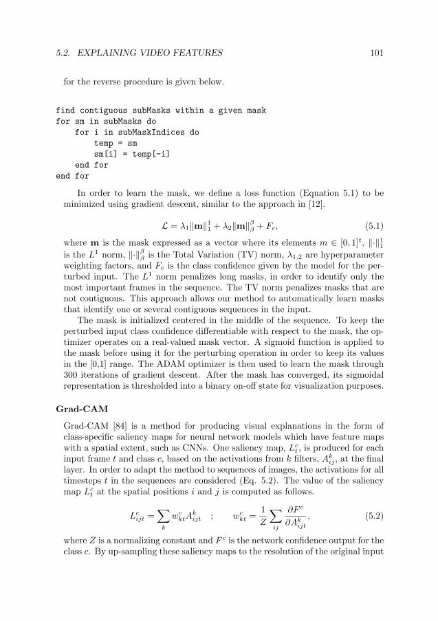
5.2. EXPLAINING VIDEO FEATURES 101
for the reverse procedure is given below.
find contiguous subMasks within a given mask
for sm in subMasks do
for i in subMaskIndices do
temp = sm
sm[i] = temp[-i]
end for
end for
In order to learn the mask, we define a loss function (Equation 5.1) to beminimized using gradient descent, similar to the approach in [12].
L = λ1‖m‖11 + λ2‖m‖ββ + Fc, (5.1)
where m is the mask expressed as a vector where its elements m ∈ [0, 1]t, ‖·‖11is the L1 norm, ‖·‖ββ is the Total Variation (TV) norm, λ1,2 are hyperparameterweighting factors, and Fc is the class confidence given by the model for the per-turbed input. The L1 norm penalizes long masks, in order to identify only themost important frames in the sequence. The TV norm penalizes masks that arenot contiguous. This approach allows our method to automatically learn masksthat identify one or several contiguous sequences in the input.
The mask is initialized centered in the middle of the sequence. To keep theperturbed input class confidence differentiable with respect to the mask, the op-timizer operates on a real-valued mask vector. A sigmoid function is applied tothe mask before using it for the perturbing operation in order to keep its valuesin the [0,1] range. The ADAM optimizer is then used to learn the mask through300 iterations of gradient descent. After the mask has converged, its sigmoidalrepresentation is thresholded into a binary on-off state for visualization purposes.
Grad-CAM
Grad-CAM [84] is a method for producing visual explanations in the form ofclass-specific saliency maps for neural network models which have feature mapswith a spatial extent, such as CNNs. One saliency map, Lct , is produced for eachinput frame t and class c, based on the activations from k filters, Akij , at the finallayer. In order to adapt the method to sequences of images, the activations for alltimesteps t in the sequences are considered (Eq. 5.2). The value of the saliencymap Lct at the spatial positions i and j is computed as follows.
Lcijt =∑k
wcktAkijt ; wckt =
1
Z
∑ij
∂F c
∂Akijt, (5.2)
where Z is a normalizing constant and F c is the network confidence output for theclass c. By up-sampling these saliency maps to the resolution of the original input

102 CHAPTER 5. EMPIRICAL PROPERTIES OF DEEP VIDEO MODELS
image, the aim is to examine what spatial data in specific frames contributed mostto the predicted class. [84]
Experiments
In this section, I will detail the training procedure for each architecture and howwe computed the saliency maps for each of the models. In ‘Comparison method’,I further present the metrics we used to compare the spatiotemporal features ofthe two models.
Training and architecture details
Both models were trained from scratch on each dataset, to ensure that the learnedmodels were specific to the relevant task. Pre-training on Kinetics can increaseperformance, but for our experiments, the models should be trained on the tem-poral tasks presented by the Something-something dataset specifically. It canbe noted that our I3D model reached comparable performance to another I3Dtrained from scratch on Something-something presented in the work of [116].
Frame sampling. Both Something-something and KTH Actions have sequencesvarying from one to almost ten seconds. As 3D CNNs require input of fixed se-quence length, all input sequences from both datasets are uniformly sub-sampledto cover the entire sequence in 16 frames (Something-something) and 32 frames(KTH Actions). The same set of sub-sampled frames is then used as input forboth architectures. Further hyperparameters are listed on the project webpage.Any remaining settings can be found in the public code repositorypublic coderepository.
I3D and Grad-CAM. I3D consists of four 3D convolutional layers, nine In-ception modules and four pooling layers (Figure 5.4). In the original setting,the temporal dimension of the input is down-sampled to L/8 frames by the finalInception module, where L is the original sequence length. In order to achieve ahigher temporal resolution in the produced Grad-CAM images, the strides of thefirst convolutional layer and the second max pooling layer are reduced to 1x2x2 inour code, producing L/2 activations in the temporal dimension. The Grad-CAMimages are produced from the gradients of the class scores with respect to thefinal Inception module.
ConvLSTM and Grad-CAM. We have not found any published ConvLSTMstrained on raw pixels, and thus conducted our own hyperparameter search for this
https://interpreting-video-features.github.io
https://github.com/interpreting-video-features/interpreting-video-features

5.2. EXPLAINING VIDEO FEATURES 103
model. The model was selected solely based on classification performance; all fea-ture investigations were conducted after this selection. The ConvLSTM used forSomething-something consists of three ConvLSTM layers (two for KTH) with 32filters, each followed by batch normalization and max pooling layers. The convo-lutional kernels used for each layer had size 5x5 and stride 2x2. The ConvLSTMlayers return the entire transformed sequence as input to the next layer. Whencalculating the Grad-CAM maps for the ConvLSTM, the final ConvLSTM layerwas used.
There is a substantial difference in the number of parameters for each model,with 12, 465, 614 for I3D and 1, 324, 014 for the three-layer ConvLSTM. Othervariants of the ConvLSTM with a larger number of parameters (up to five layers)were evaluated as well, but no significant increase in performance was observed.Also, due to the computational complexity of back-propagation through time(BPTT), the ConvLSTM variants were significantly more time demanding totrain than their I3D counterparts.
Comparison method
To study the differences in the learned spatiotemporal features of the two models,we first compute spatial saliency maps using Grad-CAM and temporal masksusing the proposed method. Once these are obtained for each model and dataset,we both examine them qualitatively and compute the quantitative metrics listedbelow. A ‘blob’ is defined as a contiguous patch within the Grad-CAM saliencymap for one frame. These salient areas were detected using the blob detectiontool from OpenCV [256]. OS, FS and RS are the softmax confidence scores for oneclass resulting from the original input, and from the freeze and reverse perturbedinput, respectively.
• Blob count: The average number of blobs (salient spatial areas, as producedby the Grad-CAM method), per frame.
• Blob size: The average size of one salient spatial area (blob), in pixels,computed across all detected blobs.
• Center distance: The average distance in pixels to the center of the framefor one blob, computed across all detected blobs.
• Mask length: The average number of salient frames per sequence, as pro-duced by the temporal mask method.
• Drop ratio: The average ratio between the drop in classification score usingthe freeze and reverse perturbations, defined as OS−FS
OS−RS , across all sequences.
• Drop difference: The average difference between the drop in classificationscore using the freeze and reverse perturbations, defined as (OS−FS)−(OS−RS) (and equivalent to RS− FS), across all sequences.

104 CHAPTER 5. EMPIRICAL PROPERTIES OF DEEP VIDEO MODELS
(a) I3D
Pred
ictio
ns
Vide
o
FCMax Pool
stride 2
32
ConvLSTM
5x5stride 2
Return All
Max Pool
stride 2
32
ConvLSTM
5x5stride 2
Return All
Max Pool
stride 2
32
ConvLSTM
5x5stride 2
Return All
(b) ConvLSTM. The max pool operation is 2D.
Figure 5.4: Schema over the I3D model (figure from [105]) and the ConvLSTMmodel.
We consider the difference and ratio between the freeze and reverse dropsas the most relevant measures of how sensitive one model was for the reverseperturbation. These metrics measure how much a confidence score drops as aresult of the reverse operation, relative to the drop as a result to the freezeoperation. The freeze operation removes information, and there should be a cleardrop for this measure. For the reverse operation, the same number of differentframes are still part of the sequence, but in the wrong order. The point of the dropratio and drop difference, then, is to measure how differently a model ‘reacted’ tothe two different perturbation. FS and RS should not be compared in absolutenumbers, since they depend on the original class confidence, OS, which often wasdifferent for the two models. Moreover, using the same number of iterations forthe optimization of the temporal mask, the two models typically reached differentfinal losses (generally lower for I3D).
Results
As a primer on these datasets, the global validation F1-scores for both archi-tectures and datasets are shown in Table 5.2. To emphasize the importance oftemporal direction between the datasets, we first conduct a test where all theinput validation sequences are entirely reversed. On Something-something, bothConvLSTM and I3D were affected drastically, while on KTH, both performedwell. Likely, this is because KTH’s classes have distinct spatial features. As ex-pected, Something-something is more time-critical than KTH. Overall, this showsthat both models are indeed globally sensitive to temporal direction, when theyneed to be. Below, we examine in detail which spatiotemporal features are learnedby the two models, and how they differ from one another.

5.2. EXPLAINING VIDEO FEATURES 105
(a) Moving something and something away from each other.
I3D OS: 0.994 ConvLSTM OS: 0.312I3D FS: 0.083 ConvLSTM FS: 0.186I3D RS: 0.856 ConvLSTM RS: 0.125
(b) Moving something and something closer to each other.
I3D OS: 0.547 ConvLSTM OS: 0.257I3D FS: 0.028 ConvLSTM FS: 0.079I3D RS: 0.053 ConvLSTM RS: 0.122I3D CS: 0.186 ConvLSTM CS: 0.002
I3D P: Moving something and something ConvLSTM P: Something fallingso they collide with each other (38) like a rock (135)
(c) Moving something and something so they pass each other.
I3D OS: 0.999 ConvLSTM OS: 0.788I3D FS: 0.002 ConvLSTM FS: 0.392I3D RS: 0.414 ConvLSTM RS: 0.537
Figure 5.5: Animated figure. Best displayed in Adobe Reader wherethe figures can be played as videos, or on the project webpage. I3D (left)and ConvLSTM (right) results for validation sequences from Something-something.The three columns show, from left to right, the original input, the Grad-CAMresult, and the input as perturbed by the temporal freeze mask. The third columnalso visualizes when the mask is on (red) or off (green), with the current framehighlighted. OS : original score (softmax output) for the guessed class, FS : freezescore, RS : reverse score, CS : score for the ground truth class when there was amisclassification and P : predicted label, if different from ground truth.

106 CHAPTER 5. EMPIRICAL PROPERTIES OF DEEP VIDEO MODELS
Model KTH Actions (Top-1) Smth-Smth (Top-1) Smth-Smth (Top-5)ConvLSTM 0.84 0.23 0.48ConvLSTM (rev.) 0.78 0.05 0.17I3D 0.86 0.43 0.73I3D (rev.) 0.80 0.09 0.27
Table 5.2: Validation F1-score per model on the two datasets. ’Rev.’ indicates thatthe validation sequences were reversed at test time.
Explainability results on Something-something
The less widely used ConvLSTM architecture could not reach the same globalperformance as the state-of-the-art I3D (Table 5.2), which also has an order ofmagnitude more parameters. Therefore, the models were only compared on se-quences from classes for which they had similar performance (Table 5.3). Weinclude a variety of per-class F1-scores, ranging from approximately 0.1 to 0.9.All are, however, well above the random chance performance of 1/174 ≈ 0.006.The reason to include a variety of performance levels when studying the extractedfeatures is to control for the general competence of the model, since a well per-forming model might extract different features than a poor one. We are interestedin the overall behavior of the models, both when they perform well and when theyperform poorly. Further, the ConvLSTM was often slightly below the I3D, evenin the performance-matched classes, making it more important to study a rangeof performances for a fair comparison.
In this section, we present an analysis of the Grad-CAM saliency maps andtemporal masks generated for each architecture on the classes listed in Table 5.3.We evaluated the models on all validation sequences from these classes (1575sequences in total). Quantitative results from the feature analysis are shown inTables 5.4-5.5 and in Figure 5.8. We display eight sample sequences in Figs.5.5-5.7 and more on the project webpage.
Trends regarding the spatial focus of the two models. We observe thatthe I3D generally focuses on contiguous, centered blobs, while the ConvLSTMattempts to find relevant spatial features in multiple smaller areas (Table 5.4).Figs. 5.5a and 5.5c show examples of this, where I3D focuses on a single regioncovering both objects, while the ConvLSTM has separate activations for the twoobjects, hands and the surface affected by the movement.
We further find that the I3D has a bias of starting its focus around the middleof the frame (Figs. 5.5-5.7), often even before the motion starts. This trendpersists throughout the sequence, as the average distance to the center of theimage for each blob in each frame is shorter for I3D (Table 5.4). The typicalbehavior for the ConvLSTM is instead to remain agnostic until the action actuallystarts (e.g., Figure 5.7a). In Figure 5.7a, the I3D maintains its foveal focus
https://interpreting-video-features.github.io

5.2. EXPLAINING VIDEO FEATURES 107
Class I3D ConvLSTMburying something in something 0.1 0.06moving something and something away from each other 0.76 0.58moving something and something closer to each other 0.77 0.57moving something and something so they collide with each other 0.16 0.03moving something and something so they pass each other 0.37 0.31moving something up 0.43 0.40pretending to take something from somewhere 0.10 0.07turning the camera downwards while filming something 0.67 0.56turning the camera left while filming something 0.94 0.79turning the camera right while filming something 0.91 0.8turning the camera upwards while filming something 0.81 0.73
Table 5.3: F1-score per class and model on the Something-something dataset.
Table 5.4: Statistics for the Grad-CAM maps for each model on eleven classesfrom the validation set of Something-something (1575 sequences, 16 frames persequence) and the whole test set of the KTH dataset (863 sequences, 32 frames persequence). The ’blobs’, i.e., the contiguous patches within each Grad-CAM map,were computed per frame, using the blob detection tool from OpenCV [256].
Model (Dataset) Blob count Blob size Center distanceI3D (Smth-smth) 1.6± 0.97 33.7± 19.6 54.4± 33.6ConvLSTM (Smth-smth) 3.6± 1.9 26.7± 24.5 96.8± 34.9I3D (KTH) 1.1± 0.5 44.0± 18.7 44.6± 19.4ConvLSTM (KTH) 32.6± 15.1 5.8± 7.0 49.9± 22.4
even after the green, round object is out of frame. In Figure 5.7b, the focussplits midway to cover both the moped and some features on the wall, while theConvLSTM focuses mainly on numerous features along the wall, as it usuallydoes in classes where the camera turns. The ConvLSTM also seems to pay moreattention to hands appearing in the clips, rather than objects (Figs. 5.5a, 5.5c,5.6a-b). Figure 5.8 shows the normalized histograms of these spatial features.The distributions for the two models differ significantly on all three measures.
Trends regarding the temporal focus of the two models. The quantita-tive results from the temporal mask experiments are shown in Table 5.5. We firstnote that the average temporal mask is shorter for the I3D. This suggests thatit has learned to react to short, specific events in the sequences. As an example,its temporal mask in Figure 5.5c is active only on the frames where the objectsfirst pass each other, and in Figure 5.5b, it is active on the frames leading to theobjects touching (further discussed in Section 5.2). Second, we note that the drop

108 CHAPTER 5. EMPIRICAL PROPERTIES OF DEEP VIDEO MODELS
Table 5.5: Statistics for the temporal masks of both models for both datasets (1575sequences for Something-something and 863 sequences for KTH).
Model (Dataset) Mask length Drop ratio Drop diff.I3D (Smth-smth) 6.2± 3.3 8.4± 47 0.2± 0.3ConvLSTM (Smth-smth) 9.9± 4.1 2.6± 6.9 0.08± 0.2I3D (KTH) 10.6± 8.5 81.4± 174 0.57± 0.34ConvLSTM (KTH) 15.2± 5.7 17.4± 45.2 0.22± 0.18
ratio and drop difference are generally higher for the I3D compared to ConvLSTM(Table 5.5), suggesting that I3D is less sensitive to the reverse perturbation.
The normalized histograms of the three measures are shown in Figure 5.8.The mask length distributions clearly have different means. For drop ratio anddrop difference, the distributions have more overlap, not least because the largestandard deviation of the drop ratio metric, in particular for the I3D. For the dropratio, if the denominator was less than a threshold (OS-RS ≤ 0.001), the samplewas filtered out, since its ratio would explode. The ratio grows large when thereis very little difference between the original confidence and the reverse perturbedconfidence, meaning when the model is not very sensitive a temporal perturbation,relative to the freeze perturbation. Given that the standard deviation is largestfor the I3D, we observe that this was more often the case for this model. At-test conducted in Scipy [257] of the difference in mean between the two modelsassuming unequal variance gives p < 10−6 for both measures. We conclude thatthere is a significant difference in mean between the two models for drop ratioand drop difference.
Class ambiguity of the Something-something dataset. The Something-something classes can be ambiguous (one class may contain another class) and,arguably, for some samples, incorrectly labeled. Examining the spatiotemporalfeatures may give insight as to how the models handle these ambiguities. Fig-ure 5.6b shows a case of understandable confusion, where I3D predicts takingone of many similar things on the table. The surface seen in the image is a tiledfloor, and the object is a transparent ruler. Once the temporal mask activatesduring the lifting motion in the last four frames, the Grad-CAM images show themodel also focusing on two lines on the floor. These could be considered similarto the outline of the ruler, which could explain the incorrect classification. Anexample of ambiguous labeling can be seen for example in Figure 5.5b, whereI3D’s classification is moving something and something so they collide with eachother and the ConvLSTM predicts pushing something with something. Although
The OS-FS ≤ 0.001 were also excluded for balance. When using 10−9 as threshold instead,the drop ratio results for Something-something were 215±6346 (I3D) and 4.9±47.6 (ConvLSTM).

5.2. EXPLAINING VIDEO FEATURES 109
the two objects in the sequence do move closer to each other, they also touch atthe end, making both predictions technically correct.
Explainability results on the KTH Actions dataset
For the KTH dataset, we make similar observations regarding temporal and spa-tial features, where the I3D generally has shorter temporal masks, as well asfewer and more centered focus areas (Table 5.4-5.5). In terms of the blob countand size, the difference is more striking between the two models on KTH thanon Something-something. This may be because there is more spatial bias in theKTH dataset, and it suffices to always focus somewhere in the middle of theframe, with an optimally sized blob, learned for the dataset. On the other hand,difference in center distance is slightly smaller for KTH between the two mod-els. This suggests that the ConvLSTM has also learned that a foveal focus isappropriate for this dataset.
In Figure 5.9a, we observe results for the class ‘handclapping’. Interestingly,the mask of each model covers at least one entire cycle of the action. The reverseperturbation affects both models very little since one action cycle is symmetricalin time for handclapping. For the ’running’ class (Figure 5.9b), we see that thetemporal mask identifies the frames in which the subject is in-frame as the mostsalient for both models, with I3D placing more focus on the subject’s legs.
A note on the temporal granularity of the two models’ feature spaces
As seen in Chapter 4, 3D CNNs and ConvLSTMs have fundamentally differentways of modeling time. In the following, we discuss two related observations: theshorter temporal masks of I3D and the fact that the classification scores after thefreeze and reverse perturbations often are lower for I3D than for the ConvLSTM.
For the I3D, all dimensions including the temporal axis of the input are pro-gressively compressed through either convolutional strides or max pooling. Thegeneral understanding of CNNs are that later layers encode higher level features.In the video explainability work by Feichtenhofer et al. [154], it is indeed shownthat the later layer units of a 3D CNN activate maximally for higher level ac-tions. The representation that is input to the prediction layer in a 3D CNN hascompressed high level motions or spatial relations through time to a shorter rep-resentation. The classification is then dependent on the presence or absence ofcertain high level features, relevant for a particular class, in this representation.If perturbing the input would alter these critical high level features, the resultingprediction might be drastically affected.
For the ConvLSTM, however, hidden states resulting from the entire inputsequence are sent to the prediction layer. Ultimately, this means that it has amore temporally fine-grained feature space than its 3D CNN counterpart. Wehypothesize that this is related to the two observed results. Due to this fine-grained and enveloping temporal feature space, the perturbation must remove
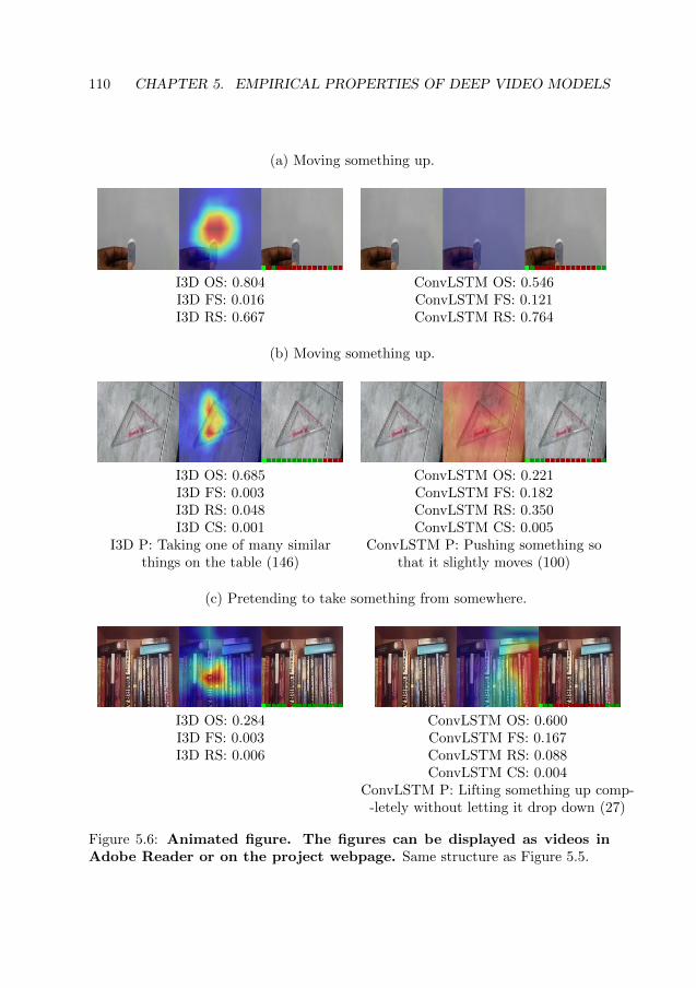
110 CHAPTER 5. EMPIRICAL PROPERTIES OF DEEP VIDEO MODELS
(a) Moving something up.
I3D OS: 0.804 ConvLSTM OS: 0.546I3D FS: 0.016 ConvLSTM FS: 0.121I3D RS: 0.667 ConvLSTM RS: 0.764
(b) Moving something up.
I3D OS: 0.685 ConvLSTM OS: 0.221I3D FS: 0.003 ConvLSTM FS: 0.182I3D RS: 0.048 ConvLSTM RS: 0.350I3D CS: 0.001 ConvLSTM CS: 0.005
I3D P: Taking one of many similar ConvLSTM P: Pushing something sothings on the table (146) that it slightly moves (100)
(c) Pretending to take something from somewhere.
I3D OS: 0.284 ConvLSTM OS: 0.600I3D FS: 0.003 ConvLSTM FS: 0.167I3D RS: 0.006 ConvLSTM RS: 0.088
ConvLSTM CS: 0.004ConvLSTM P: Lifting something up comp-
-letely without letting it drop down (27)
Figure 5.6: Animated figure. The figures can be displayed as videos inAdobe Reader or on the project webpage. Same structure as Figure 5.5.

5.2. EXPLAINING VIDEO FEATURES 111
(a) Turning the camera downwards while filming something.
I3D OS: 1.000 ConvLSTM OS: 0.158I3D FS: 0.001 ConvLSTM FS: 0.063I3D RS: 0.011 ConvLSTM RS: 0.093
(b) Turning the camera upwards while filming something.
I3D OS: 0.990 ConvLSTM OS: 0.806I3D FS: 0.001 ConvLSTM FS: 0.177I3D RS: 0.000 ConvLSTM RS: 0.181
Figure 5.7: Animated figure. Best displayed in Adobe Reader where thefigures can be played as videos or on the project webpage. Same structureas Figure 5.5.
larger sub-sequences from the data to obscure enough information through timeto cause a large change in prediction score, possibly accounting for the longertemporal masks observed for ConvLSTM. Furthermore, as we penalize the lengthof the mask during optimization, the resulting converged mask is often too shortto fully bring down the classification score of the ConvLSTM method. Examplesof where the freeze score is brought close to, or below, 0.1 are when the mask isnearly or fully active, as seen in Figs. 5.5b, 5.6a and 5.7a.
Discussion and summary
In this section, I have presented the first comparison of the spatiotemporal infor-mation used by 3D CNN and ConvLSTM-based models in action recognition. Wehave seen indications that the difference in temporal modeling has consequencesfor what features the two models learn. We have also seen that the temporalmask is capable of identifying salient frames in sequences, such as one cycle ofa repeated motion. Using the proposed temporal mask method, we presented

112 CHAPTER 5. EMPIRICAL PROPERTIES OF DEEP VIDEO MODELS
(a)
(b)
Figure 5.8: Normalized histogram results for the Grad-CAM and temporal maskanalysis for the I3D (orange) and ConvLSTM (blue) networks. The histogramscorrespond to the results in Tables 5.4-5.5.
empirical evidence that I3D on average focuses on shorter and more specific se-quences than the ConvLSTM. On average, our experiments showed that I3D alsotends to focus on fewer or a single contiguous spatial patch closer to the centerof the image, instead of smaller areas on several objects like the ConvLSTM.
It should be noted that focusing in the center of the frame is appropriate forthe Something-something dataset, since most of the relevant action is centered (itcontains a center bias). I3D is an efficient learner which can economically figureout what is most strategic to focus on. On the other hand, this may not be abehavior that generalizes well. Further, when comparing the effect of reversing themost salient frames or removing motion through ‘freezing’ them, the ConvLSTMexperiences a relatively larger decrease in prediction confidence than I3D uponreversal. Taken together, these findings suggest that the ConvLSTM overall ismore attentive to the actual temporal patterns than the I3D.
There is still much to explore in the patterns lying in temporal dependencies.In this section, we compared one instance each of the two model types, as a firstinvestigation of whether there may be qualitative differences in the features ofdifferent video models. In the next Section (5.3), a study of qualitative behavioracross a larger number of instances per model type will be conducted.
It would further be of interest to extend the study to other datasets where

5.2. EXPLAINING VIDEO FEATURES 113
(a) Handclapping, Subject 18.
I3D OS: 0.999 ConvLSTM OS: 0.996I3D FS: 0.026 ConvLSTM FS: 0.997I3D RS: 0.999 ConvLSTM RS: 0.996
(b) Running, Subject 25.
I3D OS: 0.993 ConvLSTM OS: 0.669I3D FS: 0.208 ConvLSTM FS: 0.339I3D RS: 0.999 ConvLSTM RS: 0.605
Figure 5.9: Animated figure. The figures can be displayed as videos inAdobe Reader. Explainability results example on the KTH Actionsdataset. Same structure as Figure 5.5.
temporal information is important, e.g., Charades [128]. Other possible futurework includes evaluating the effect of other noise types beyond ‘freeze’ and ‘re-verse’. We hope that this empirical study can guide future development andunderstanding of deep video models.
Last, it is desirable that a model can be trained with as little data as possible,for sustainability- as well as explainability reasons. 3D CNNs do not representvideo (time) in a physically sound way, treating it as a third spatial dimension.In our view, this is often made up for using large amounts of data and brute-force learning of its correlations, as most state-of-the-art video CNNs are fromindustry, trained on hundreds of GPUs, e.g., SlowFast [115]. For efficiency, itis important that the representation learned by the model should correspond tothe world, and that variables that are uncorrelated in the world remain so in themodel. With our evaluation framework it will be possible to gain further insightinto what state-of-the-art video models have actually learned.
In Section 5.3, we will continue the investigation of the generalizability of thespatiotemporal features learned by principally different video models.

114 CHAPTER 5. EMPIRICAL PROPERTIES OF DEEP VIDEO MODELS
5.3 Frame dependency modeling matters for cross-domainrobustness in action recognition
In Section 5.2, we raised questions about how the features of the 3D CNN wouldfare in the wild. These tended to be more center biased and to be based onshorter parts of the video clips for its decisions, as compared to the ConvLSTM.In this section, we conduct an empirical study on how the choice of frame depen-dency modeling in action recognition affects cross-domain robustness, which haspreviously not been studied.
We further introduce a novel, lightweight, dataset which allows for investiga-tion of both temporal shape modeling ability and domain generalization, calledthe Temporal Shape dataset. We provide the first discussion and experimentson shape vs. texture bias (following the nomenclature by Geirhos et al. [13]) indeep video models. In connection to this work, we also have made shape andtexture versions of the Diving48 dataset public, allowing studies on whether avideo model has learned to rely more on (temporal) shape or texture.
As argued in Chapter 4, one of the most fundamental questions when it comesto video understanding in computer vision, or computer vision in general, is howto model the dependency between frames. The system should ideally be ableto gather how particular frames relate to others, and which shapes and objectshave changed or persisted over time. With this knowledge, it can start to inferrelationships at a higher level, such as object-object or agent-object relationships,and, for example, distinguish a suddenly appearing fine-grained motion. In spiteof the essentiality of this question, it has almost disappeared from action recog-nition articles, possibly in the race to improve on the classification benchmarks.In this section, we perform an empirical study of the cross-domain generalizationabilities of video models, comparing ones that recur, attend or convolve acrossthe temporal dimension. The aim of the study is to investigate whether there areinherent differences in what is learned, pertaining to generalizability, dependingon which method is chosen for temporal modeling. In our work, we investigatethe empirical consequences of these trends for time-critical video modeling.
Experiment design
Here, we give an overview of the methodology and experiments conducted on thetwo datasets: Temporal Shape and Diving48.
Main idea. In all of our experiments, we begin by training on one specificdomain, while validating on a held-out dataset from the same domain. We selectthe model that performs best on the validation set, and then proceed to evaluateit on other domains that are different in some respects but share the same task.Following Chen et al. [166], the domain we train on will be referred to as the sourcedomain, and the unseen domains that we evaluate on, as the target domains.

5.3. FRAME DEPENDENCY MODELING MATTERS FOR CROSS-DOMAINROBUSTNESS IN ACTION RECOGNITION 115
The aim of this section is to study how principally different ways of modelingtemporal dependency affect the out-of-domain generalization ability. In a nut-shell, we will empirically compare different video models on a number of domaintransfer tasks. To measure cross-domain robustness, we define the robustnessratio (rr.) for one model as the ratio between its accuracy on a target domainand its best validation accuracy on the source domain. When the target domaincorresponds to the true task, this number should ideally be close to one (higheris better). It can be noted that the rr. is a heuristic metric, which builds onthe observation that the performance on the in-domain validation set typically ishigher than on other domains. If the performance on the validation set is poorto begin with, the rr. is less informative.
Method common to all experiments. We ensure that all sequences are ofequal length by uniform sub-sampling of the frames, since a fixed input size isrequired for the input to both 3D CNNs and attention-based models. There areother frame sampling methods, which can be used as augmentation, or as informedpriors (e.g., the TimeSformer only samples the middle frames during inferencein [179]), but in our study we are comparing the basic functionality of models.No pre-training, dropout, or data augmentation is applied in our experiments,except for 50% chance of horizontal flipping of the clips on Diving48. Coderelated to neural networks was written in PyTorch [258] using Lightning [259].All experiments have been run using the same random seed throughout the study.
Models
We will compare ConvLSTMs, 3D CNNs and Video Transformers, since thesepresent three principally different temporal modeling approaches. For the latter,we will use the TimeSformer [179], because it recently achieved state-of-the-artresults on a number of action recognition benchmarks. Since there do not existstate-of-the-art video models based fully on ConvLSTM-layers, we deem it fairto compare ConvLSTMs both to simple and state-of-the-art video models of theother two kinds.
It is a challenging task to compare neural network models which have prin-cipally different architectures. In our work, we decided on controlling for threedifferent factors: the layer structure (i.e., the number and expressivity of hierar-chical abstractions), the performance on a particular dataset and the number oftrainable parameters. The experiments were designed prior to running them, tokeep the process as unbiased as possible.
A ConvLSTM video model in this work is a model fully based on ConvLSTMlayers, with a classification head on top, similarly to the model in Section 5.2. Itis also the same type of model as in Sections 3.2-3.3, but in one stream (of RGBinput). As for the TimeSformer, we use the TimeSformer-PyTorch PyPi library[260], mainly with the standard model settings which are given in the repository.We note again that we do not use pre-training, advanced data augmentation,

116 CHAPTER 5. EMPIRICAL PROPERTIES OF DEEP VIDEO MODELS
nor averaging over multiple predictions, which results in a lower performance onDiving48 for this model than its state-of-the-art results. Finally, for the 3D CNNs,we use models which consist fully of 3D convolutional layers, similar to standard2D CNNs, including batch normalization and pooling, with a classification headon top. More details regarding the architecture for each experiment will follow.
Experiments on the Temporal Shape dataset
In the Temporal Shape experiments, we use small models, and control for layerstructure by letting the compared models have three layers each of analogousblocks, with the same number of hidden units in each. One block for the ConvL-STM and 3D CNN consists of a model-specific layer including activations (tanhfor the ConvLSTM layer and ReLU for the 3D convolutional layer), a max poolinglayer (2D pooling for the ConvLSTM and 3D pooling for the 3D CNN), followedby batch normalization. The ConvLSTM and 3D CNN models used the sameconvolutional kernel sizes in all three layers (3 × 3). For the TimeSformer, weused one TimeSformer layer as one block, and the latent dimension for each at-tention head, Dh, as the number of hidden units, since these were similar in scale.Further details can be found in the code repository. In the online Appendix, weadditionally present results using a single attention head (Dh = 1), where thepatch embedding size D instead assumes the role of the number of hidden units.
Since the dataset is small, we are using lightweight models for this experiment,consisting of ten trials in total. For all models, we are using three blocks (orTimeSformer layers). For each experiment, we increase the number of hiddenunits, h, in each of the model-specific layers, where h ∈ {1, 2, 3, 5, 8, 12, 16, 24, 32,
48}. For each of the ten experiments of varying model sizes, we train the modelson the five-class task on the source domain for 100 epochs, with ten epochs ofearly stopping patience. For the TimeSformer, these numbers were 300 (maxi-mum number of epochs) and 100 (early stopping), because it is larger, with lessinductive biases and requires more epochs to train than the other two types ofmodels.
We then evaluate the model which performed the best on the source domainvalidation set on different target domains with the same classification task. Forthe Temporal Shape dataset, recall that we have four different domains, rangingfrom less to more texture in each frame (Section 5.1 and Figure 5.1). Experimentswere conducted in two ‘directions’, from less texture to more texture (training on2Dot), and from more texture to less texture (training on MNIST-bg). The Dh
and D hyperparameters needed to be even numbers in the TimeSformer imple-mentation; thus, the TimeSformer was not included in the trials for h ∈ {1, 3, 5}.
Training on the temporal shape data is light-weight compared to real videodata, and runs fast (in the minutes-range for the model sizes we evaluated) onone GPU card. We train with a batch size of 64, a hyperparameter that was fixedin all Temporal Shape experiments.

5.3. FRAME DEPENDENCY MODELING MATTERS FOR CROSS-DOMAINROBUSTNESS IN ACTION RECOGNITION 117
Experiments on Diving48
Training. We are deliberately avoiding bells and whistles when training modelson Diving48. All three models are trained with the same SGD optimizer, cross-entropy loss, and a constant learning rate of 0.001. Each model is trained for 500epochs maximally, with an early stopping patience of 30 epochs if the validationperformance does not improve. The only data augmentation used is horizontalflipping of 50% probability for the entire clip. The models are trained usingPyTorch Lightning’s ddp parallelization scheme across eight A100 GPUs, with abatch size of 8 and a clip length of 32 uniformly sampled frames, at 224×224.
Given that the purpose of our experiments is not to optimize classificationperformance, we evaluate the models at different levels of performance, rang-ing from 30% to 50% accuracy. Some of the advanced state-of-the-art methodstoday, including pre-training and heavy data augmentation, obtain up to 80%performance on Diving48, but when the dataset was introduced in 2018, andstandard video methods were tested off-the-shelf on it, the best result was 27%accuracy [10]. Thus, the range of 30-50% is reasonably well-performing, and wellabove random (which is at 2.1%).
Experiments. We conduct three different kinds of experiments on the Div-ing48 dataset across different performance levels, namely: control for layer struc-ture and performance (experiments a-c), and control for performance for the bestperforming variants (experiment d), and control for number of parameters andperformance (experiments e-h).
a-c. Controlling for layer structure and performance. In this experiment, we letthe models have four layers (blocks) of abstraction, with 128 hidden units in each.As in the Temporal Shape experiments, we treat Dh as the hidden unit analogyfor the TimeSf, since it is most similar in scale. We evaluate checkpoints of themodels at different performance levels: 30%, 35%, and 38.3% accuracy. The last,and very specific accuracy, was chosen because it was the limiting, highest per-formance by the 3D CNN in this experiment. Having the same layer structuregives rise to a varying number of parameters for each type of model. Here, the3D CNN has 10.6M parameters, ConvLSTM has 14.3M parameters, and TimeSfhas 85M.
d. Controlling for performance only. Here, we compare models at their best per-formance, after hyperparameter search. Since it was not possible to train TimeSfto a higher accuracy than 39.7% in all variants we tried, this experiment wasonly conducted with the 3D CNN and ConvLSTM. A complete list of the vari-ants we attempted with the TimeSformer can be found in the online Appendix.The ConvLSTM had four blocks of 128 hidden ConvLSTM units each (14.3M pa-rameters). The 3D CNN was an 11-layer VGG-style model (23.3M parameters).

118 CHAPTER 5. EMPIRICAL PROPERTIES OF DEEP VIDEO MODELS
Best val. 5dot MNIST MNIST-bg
20
30
40
50
60
70
80
90
100
a) Training on 2Dot
Best val. MNIST 5Dot 2Dot
20
30
40
50
60
70
80
90
100
b) Training on MNIST-bg
3D CNNConvLSTMTimeSf
Figure 5.10: Average results (% acc.) across trials with varying numbers of hiddenunits per layer. The shaded area corresponds to standard deviation across thetrials. Detailed data corresponding to this plot can be found in Tables 5.6 and 5.7.
The checkpoints used were both at exactly 50.07% validation accuracy.
e-h. Controlling for number of parameters and performance. Here, we have chosenmodels with a similar amount of trainable parameters, in this case 14M. To arriveat this number of parameters for TimeSf, its depth was reduced from 12 to 11,and Dh and D were halved, to 32 and 256, respectively, relative to the defaultmodel. The ConvLSTM has four blocks with 128 units in each, and the 3D CNNhas six blocks with 128 units in each.
Results and discussion
Having presented the experimental design for both datasets, next, I discuss ourempirical findings, first on the Temporal Shape dataset, and then on Diving48and its modified domains.
Temporal Shape
Training on 2Dot. The results are shown in Fig. 5.10 a (with details in Tables5.6). Although the 3D CNN generally obtains higher results on the source domainvalidation set, the rr. is generally higher for ConvLSTM; it drops less compared toits original result when tested on unseen domains with increasingly noisy texture.
Robustness ratio vs. model size. In Fig. 5.11 we have plotted the rr. for thethree target domains when training on 2Dot. For 5Dot, the rr. for ConvLSTMdecreases slightly with the model complexity, whereas the 3D CNN and TimeSf,in contrast, increase the rr. along with increased model complexity. In the MNISTdomain, which is further from the validation domain, the upward trend for the3D CNN and TimeSf is broken. For the most challenging domain, MNIST-bg, the

5.3. FRAME DEPENDENCY MODELING MATTERS FOR CROSS-DOMAINROBUSTNESS IN ACTION RECOGNITION 119
Tab
le5.
6:T
est
resu
lts
(%ac
cura
cy)
wh
entr
ain
ing
on2D
ot(2
-vis
the
bes
tva
lid
atio
nre
sult
onth
eso
urc
ed
omain
2D
ot)
and
eval
uat
ing
onth
eth
ree
un
seen
dom
ain
s,w
hile
incr
easi
ng
the
nu
mb
erof
hid
den
un
its
per
laye
r.
3D
CNN
ConvLSTM
Tim
eSf
#h
2-v
5M
M-b
g2-v
5M
M-b
g2-v
5M
M-b
g
170.7
53.6
46.6
41.8
61.2
49.0
20.6
20.8
281.0
43.0
34.6
27.0
52.4
52.6
35.8
78.1
30.8
22.6
21.8
17.6
385.3
45.2
28.6
27.0
52.5
36.0
36.0
18.0
586.0
63.8
33.2
18.4
44.6
38.0
29.6
29.6
893.2
81.2
48.6
36.2
53.5
41.6
32.8
23.2
72.7
53.4
38.4
22.2
12
93.5
70.6
45.2
23.2
53.5
51.6
35.8
27.2
70.5
44.6
36.6
17.6
16
94.1
75.4
44.0
22.8
91.8
60.6
52.4
22.8
81.3
52.0
47.2
18.6
24
93.9
82.2
48.4
22.8
95.8
55.4
46.4
22.8
73.8
45.4
38.8
20.0
32
93.8
70.0
41.8
27.4
94.7
71.0
59.2
26.8
72.7
62.6
43.6
17.6
48
92.4
84.6
31.2
22.8
94.4
58.8
50.4
22.8
71.1
56.2
42.0
18.6
Avg.
88.4
67.0
40.2
26.9
69.4
51.5
39.9
23.4
74.3
49.3
38.3
18.9
Std
.±
7.7
5±
15.2
±7.5
8±
7.0
3±
21.7
±10.9
±11.8
±3.5
7±
3.9
5±
10.2
±8.1
3±
1.7
0
Avg.rr.↑
0.7
53
0.4
58
0.3
12
0.770
0.587
0.368
0.6
67
0.5
18
0.2
55
Std
.rr.
±0.1
3±
0.0
97±
0.1
1±
0.1
4±
0.1
1±
0.1
3±
0.1
5±
0.1
1±
0.0
3

120 CHAPTER 5. EMPIRICAL PROPERTIES OF DEEP VIDEO MODELS
Tab
le5.
7:T
est
resu
lts
(%ac
cura
cy)
wh
entr
ain
ing
and
vali
dat
ing
onM
NIS
T-b
g(M
-bg-
vis
the
bes
tva
lid
atio
nre
sult
on
the
sou
rce
dom
ain
MN
IST
-bg)
,an
don
the
thre
eu
nse
end
omai
ns,
wh
ile
incr
easi
ng
the
nu
mb
erof
hid
den
un
its
per
laye
r.
3D
CN
NC
onvL
ST
MT
imeS
f
#h
M-b
g-v
M5
2M
-bg-v
M5
2M
-bg-v
M5
2
186.6
86.0
26.6
26.0
81.2
82.0
27.0
23.6
290.7
91.0
28.0
24.0
84.3
86.8
28.8
22.2
67.0
67.4
38.8
28.4
394.1
94.4
29.8
27.2
85.0
83.4
29.6
24.6
593.9
93.6
28.0
26.0
92.4
91.0
30.2
24.8
895.5
96.8
28.6
25.4
92.8
91.6
31.2
25.2
84.5
83.8
36.4
28.0
12
96.5
96.4
27.8
27.0
95.5
96.6
30.0
25.8
90.1
87.4
42.0
38.2
16
97.6
98.0
32.2
26.6
90.7
89.4
27.8
23.0
89.7
90.6
43.6
38.8
24
97.3
97.6
28.8
24.2
93.8
91.2
30.0
24.0
92.6
93.0
44.8
36.0
32
96.9
97.8
29.0
27.0
93.6
91.2
32.8
24.4
91.9
89.6
40.4
33.6
48
96.7
96.8
30.4
25.6
93.8
92.6
31.0
22.4
91.7
91.8
43.4
43.2
Avg.
94.6
94.8
28.9
25.9
90.3
89.6
29.8
24.0
86.8
86.2
41.3
35.2
Std
.±
3.5
0±
3.8
2±
1.5
7±
1.1
3±
4.9
5±
4.3
9±
1.6
8±
1.1
9±
9.1
3±
8.8
4±
2.9
9±
5.5
9
Avg.
rr.↑
1.0
00.3
06
0.2
74
0.9
92
0.3
31
0.2
66
0.9
94
0.4
80
0.4
05
Std
rr.
±0.0
06±
0.0
12±
0.0
14
±0.0
19±
0.0
14±
0.0
16
±0.0
16±
0.0
49±
0.0
47
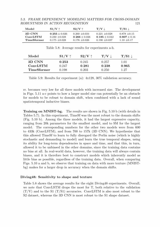
5.3. FRAME DEPENDENCY MODELING MATTERS FOR CROSS-DOMAINROBUSTNESS IN ACTION RECOGNITION 121
Model S1/V ↑ S2/V ↑ T/V ↓ T/S1 ↓
3D CNN 0.255± 0.026 0.260 ±0.034 0.221 ±0.028 0.878 ±0.15ConvLSTM 0.230 ±0.028 0.266± 0.026 0.185± 0.042 0.807± 0.16TimeSformer 0.175 ±0.028 0.176 ±0.026 0.190 ±0.037 1.10 ±0.17
Table 5.8: Average results for experiments a-h.
Model S1/V ↑ S2/V ↑ T/V ↓ T/S1 ↓3D CNN 0.253 0.245 0.257 1.01ConvLSTM 0.247 0.281 0.238 0.965TimeSformer 0.198 0.203 0.250 1.27
Table 5.9: Results for experiment (a): 4x128, 30% validation accuracy.
rr. becomes very low for all three models with increased size. The developmentin Figs. 5.11 a-c points to how a larger model size can potentially be an obstaclefor models to be robust to domain shift, when combined with a lack of soundspatiotemporal inductive biases.
Training on MNIST-bg. The results are shown in Fig. 5.10 b (with details inTables 5.7). In this experiment, TimeSf was the most robust to the domain shifts(Fig. 5.10 b). Among the three models, it had the largest expressive capacity,ranging from 20k parameters for the smallest model, and to 9M for the largestmodel. The corresponding numbers for the other two models were from 600to 433k (ConvLSTM), and from 700 to 157k (3D CNN). We hypothesize thatthis allowed TimeSf to learn to fully disregard the Perlin noise (which is highlystochastic and demanding to model) and learn the true temporal shapes, usingits ability for long-term dependencies in space and time, and that this, in turn,allowed it to be unbiased in the other domains, since the training data containsno bias at all. In real-world data, however, the training data will always containbiases, and it is therefore best to construct models which inherently model aslittle bias as possible, regardless of the training data. Overall, when comparingFigs. 5.10 a and b, we observe that training on data with more texture (MNIST-bg) makes for a larger drop in accuracy when the domain shifts.
Diving48: Sensitivity to shape and texture
Table 5.8 shows the average results for the eight Diving48 experiments. Overall,we note that ConvLSTM drops the most for T, both relative to the validation(T/V) and to the S1 (T/S1) accuracies. ConvLSTM is also most robust to theS2 dataset, whereas the 3D CNN is most robust to the S1 shape dataset.

122 CHAPTER 5. EMPIRICAL PROPERTIES OF DEEP VIDEO MODELS
Figure 5.11: Robustness ratio (rr.) (↑) when training on 2Dot, vs. number ofhidden units per layer. X-axis and legend are shared across the three plots. Higheris better. The target domain is progressively further away from the source insubplots a-c.
Model S1/V ↑ S2/V ↑ T/V ↓ T/S1 ↓3D CNN 0.230 0.233 0.243 1.06ConvLSTM 0.217 0.271 0.199 0.919TimeSformer 0.154 0.152 0.190∗ 1.24
Table 5.10: Results for experiment (b): 4x128, 35% validation accuracy. * when alow T/V result is not accompanied by T/S1 < 1.
Experiments a-d. In experiments a-c (Fig. 5.12), where we vary the validationaccuracy on the source domain between 30% and 38.3% on a fixed architectureof four layers with 128 units each, both TimeSf and the 3D CNN performs betteron T than on S1 and S2, even if only the two latter contain actual class evidence.Tables 5.9-5.11 show that T/S1 > 1 in all three experiments for these two models,also visible in Figure 5.12. In Tables 5.10-5.11, TimeSf has the best metrics forT/V (drops the most for T relative to the validation set). This can be explained

5.3. FRAME DEPENDENCY MODELING MATTERS FOR CROSS-DOMAINROBUSTNESS IN ACTION RECOGNITION 123
Bv. S1 S2 T
5 · 10−2
0.1
0.15
0.2
0.25
0.3
a) 4x128, 30%
3D CNNConvLSTMTimeSf
Bv. S1 S2 T
5 · 10−2
0.1
0.15
0.2
0.25
0.3
0.35
b) 4x128, 35%
3D CNNConvLSTMTimeSf
Bv. S1 S2 T
5 · 10−2
0.1
0.15
0.2
0.25
0.3
0.35
c) 4x128, 38.3%
3D CNNConvLSTMTimeSf
Bv. S1 S2 T
0.1
0.2
0.3
0.4
0.5
d) Best vars., 50%
3D CNNConvLSTM
Figure 5.12: Accuracy drops for Diving48, from the source to the target domains,experiments a-d. Bv. means best result in the validation domain.
Model S1/V ↑ S2/V ↑ T/V ↓ T/S1 ↓3D CNN 0.219 0.219 0.237 1.09ConvLSTM 0.279 0.308 0.187 0.669TimeSformer 0.155 0.155 0.175∗ 1.13
Table 5.11: Results for experiment (c): 4x128, 38.3% validation accuracy. * whena low T/V result is not accompanied by T/S1 < 1.
by its overall large drops, rather than being robust to texture bias, which is mostclearly visible in Figure 5.12 a-c. For T/V to be a meaningful metric, T/S1 shouldbe < 1. Therefore, we have put asterisks on boldface T/V results which are notaccompanied by T/S1 < 1.
In contrast, ConvLSTM clearly drops for T. TimeSf is large here, at 85M pa-rameters, whereas the 3D CNN is interestingly quite small at 10.6M parameters.This suggests that it is not only the parameter count that causes susceptibil-ity for overfitting, but possibly that there are innate tendencies to overfitting inthe choice of spatiotemporal (frame dependency) modeling. A recurrent modelnecessarily takes each timestep into account, in the sense that each timestep isnon-linearly registered in the hidden state. We hypothesize that this enables itto register motion changes over time more carefully, and count these as salient,when that is the case (as it should be for Diving48). This also relates to thediscussion on the temporal granularity of the feature space of RNNs compared to3D CNNs in Section 5.2.
In experiment d, where we compare a ConvLSTM and a 3D CNN at 50.07%validation accuracy, the 3D CNN does not improve on the texture dataset relativeto S1 and S2, but the drop is larger for ConvLSTM. To increase its validationperformance, it was necessary to scale up the size of the 3D CNN – here, it has

124 CHAPTER 5. EMPIRICAL PROPERTIES OF DEEP VIDEO MODELS
Model S1/V ↑ S2/V ↑ T/V ↓ T/S1 ↓3D CNN 0.234 0.242 0.191 0.815ConvLSTM 0.232 0.248 0.136 0.586
Table 5.12: Results for experiment (d): best variants, 50% validation accuracy.
S1 S2 T
Model Top-1 Top-5 Top-1 Top-5 Top-1 Top-5
ConvLSTM 0.4 1.0 0.4 1.0 0.0 0.63D CNN 0.4 0.8 0.4 0.6 0.0 0.8TimeSf 0.4 0.4 0.2 0.4 0.0 0.2
Table 5.13: Qualitative example with predictions on five random clips from class34, made by the model instances from experiment c) (38.3% acc.).
23.3M trainable parameters, compared to the 14.3M parameters of ConvLSTM.The larger number of parameters might contribute to its relatively overfitted ten-dencies. However, this is the most realistic scenario to evaluate a 3D CNN, sincethe state-of-the-art versions are typically deep (>10 layers) and have more than20M parameters (25M for I3D, 60M for SlowFast), as noted in Chapter 4. Thisraises concern that when a large model optimizes its performance on one domain,it may have difficulties to be robust in others.
Qualitative examples from experiment c. Table 5.13 shows a breakdown ofthe models’ predictions on five randomly selected clips from a randomly chosenclass (34). The models used here are the instances from experiment c, which areall at 38.3% accuracy. Top-1 accuracy being equal between ConvLSTM and the3D CNN, we note that ConvLSTM has 100% top-5 accuracy for both S1 and S2,whereas the 3D CNN has 80% and 60%. This becomes interesting when lookingat the texture (T) results, where the top-5 accuracy of the 3D CNN remains at80%, whereas ConvLSTM drops to 60%.
Each label of Diving48 has four attributes: takeoff, somersault, twist andflight position. Looking closer at the top-1 predictions for both S1 and S2 for thefive clips (Table 5.14), we study how many attributes are correct in the misclas-sifications for each model. Class 34 has the attribute values inward takeoff, 2.5somersault, no twist and tuck flight position. For ConvLSTM, the misclassifica-tions of class 34 are 8, 20, 35 and 44, where 8, 35 and 44 all contain 3/4 correctattributes, and 20 contains 1/4 correct attributes (no twist). For the 3D CNN,only two predictions (32, 35) obtain three correct attributes, and for TimeSf,the best misclassification has only two correct attributes. This suggests that the3D CNN and TimeSf have modeled the classes in terms of the true attributesto a lesser extent than ConvLSTM, i.e., ConvLSTM has learned more relevanttemporal patterns.

5.3. FRAME DEPENDENCY MODELING MATTERS FOR CROSS-DOMAINROBUSTNESS IN ACTION RECOGNITION 125
Top-1 predictionsModel S1 S2 Misclassifications Correct attr.
ConvLSTM [34, 34, 35, 8, 20] [34, 34, 44, 8, 20] 8, 20, 35, 44 10/163D CNN [34, 19, 21, 35, 34] [34, 32, 21, 21, 34] 19, 21, 32, 35 8/16TimeSf [34, 12, 34, 47, 20] [31, 12, 34, 47, 20] 12, 20, 31, 47 5/16
Table 5.14: Top-1 predictions and misclassifications by the models, same qualitativeexample as in Table 5.13 (class 34). Each class has four attributes, and the Correctattributes column shows how many attributes were correct for the misclassifications.
S1 S2 T
Model Top-1 Top-5 Top-1 Top-5 Top-1 Top-5
ConvLSTM 0.0 0.2 0.0 0.2 0.0 0.03D CNN 0.2 0.2 0.2 0.2 0.2 0.2TimeSf 0.2 0.6 0.2 0.4 0.0 0.2
Table 5.15: Qualitative example with predictions on five random clips from class12, made by the model instances from experiment c) (38.3% acc.).
Additional qualitative examples were chosen from three more randomly se-lected classes: 12, 22 and 45. Similarly as for class 34, for each of the classes, weselect five random clips for evaluation of the three different models. The check-points are still taken from experiment c. We note their top-1 and top-5 accuracy,and how many attributes they are correct in for each clip. In Tables 5.16, 5.18and 5.20, we see that the ConvLSTM still achieves the largest proportion of cor-rect attributes in the misclassifications for these three classes. Further similar tothe first example of class 34, the 3D CNN comes second, and TimeSf last.
In Tables 5.15, 5.17 and 5.19, the trends regarding the top-1 and top-5 accu-racy on the different datasets are slightly less clear. We observe that for class 12and 45 (Tables 5.15 and 5.19), ConvLSTM and TimeSf drop the clearest in top-5performance on T relative to S1 and S2. On the other hand, for class 22 (Table5.17), the top-5 accuracy is relatively improved on T compared to S1 and S2 forConvLSTM and the 3D CNN, whereas TimeSf is unchanged. We inspected theseclips, to verify that the segmentation had not failed, which it had not. However,the ConvLSTM is still the only one out of the three to have 20% in top-1 accuracyboth for S1 and S2 on class 22, dropping to 0 in top-1 on T (Table 5.17). Last, forclass 45, the ConvLSTM has the best results on S1 and S2 (20% top-5 accuracy)out of the three models, where the others have 0% accuracy, except for 20% top-5accuracy for the 3D CNN on the texture dataset.
Experiments e-h.
The results for experiments e-h, where the number of trainable parameters andperformance are fixed, are shown in Fig. 5.13. Here, the 3D CNN is the mostrobust out of the three, although ConvLSTM approaches the 3D CNN and drops

126 CHAPTER 5. EMPIRICAL PROPERTIES OF DEEP VIDEO MODELS
Top-1 predictionsModel S1 S2 Misclassifications Correct attr.
ConvLSTM [35, 26, 45, 26, 21] [27, 26, 45, 14, 21] 14, 21, 26, 27, 35, 45 14/243D CNN [3, 20, 12, 5, 44] [3, 20, 12, 5, 34] 3, 5, 20, 34, 44 8/20TimeSf [22, 33, 12, 31, 14] [22, 33, 12, 31, 14] 14, 22, 31, 33 5/16
Table 5.16: Top-1 predictions and misclassifications by the models, same qualitativeexample as in Table 5.15 (class 12). Each class has four attributes, and the Correctattributes column shows how many attributes were correct for the misclassifications.
S1 S2 T
Model Top-1 Top-5 Top-1 Top-5 Top-1 Top-5
ConvLSTM 0.2 0.2 0.2 0.2 0.0 0.63D CNN 0.0 0.4 0.2 0.6 0.0 0.8TimeSf 0.0 0.2 0.0 0.2 0.0 0.2
Table 5.17: Qualitative example with predictions on five random clips from class22, made by the model instances from experiment c) (38.3% acc.).
Top-1 predictionsModel S1 S2 Misclassifications Correct attr.
ConvLSTM [26, 26, 35, 22, 21] [26, 26, 35, 22, 21] 21, 26, 35 5/123D CNN [29, 7, 26, 28, 0] [29, 22, 26, 26, 0] 0, 7, 26, 28, 29 7/20TimeSf [15, 27, 46, 44, 34] [15, 27, 46, 44, 34] 15, 27, 34, 44, 46 5/20
Table 5.18: Top-1 predictions and misclassifications by the models, same qualitativeexample as in Table 5.17 (class 22). Each class has four attributes, and the Correctattributes column shows how many attributes were correct for the misclassifications.
more steeply for the texture dataset in experiment h), where the performanceis highest (45% acc.). TimeSf drops from 30% and 35% to almost 5% accuracyin experiments e-f, but the result is not better for the texture dataset here (incontrast to its texture results in experiments a-c). This suggests that TimeSf ismore likely to display texture bias when it has a larger amount of parameters, asit does in experiments a-c.
Results summary and discussion
This section has shown indications that using more inductive biases for temporalmodeling, such as recurrence or convolutions, helps with cross-domain robustnessin temporally challenging video classification tasks. An explanation supportedby our findings is that such models display less texture bias than the TimeS-former. In particular, the convolutional-recurrent ConvLSTM model was themost cross-domain robust on the modified domains of Diving48 and on TemporalShape when training on 2Dot. When training on the noisy MNIST-bg domain,

5.3. FRAME DEPENDENCY MODELING MATTERS FOR CROSS-DOMAINROBUSTNESS IN ACTION RECOGNITION 127
S1 S2 T
Model Top-1 Top-5 Top-1 Top-5 Top-1 Top-5
ConvLSTM 0.0 0.2 0.0 0.2 0.0 0.03D CNN 0.0 0.2 0.0 0.0 0.0 0.2TimeSf 0.0 0.0 0.0 0.0 0.0 0.0
Table 5.19: Qualitative example with predictions on five random clips from class45, made by the model instances from experiment c) (38.3% acc.).
Top-1 predictionsModel S1 S2 Misclassifications Correct attr.
ConvLSTM [26, 21, 12, 35, 27] [26, 21, 12, 35, 44] 12, 21, 26, 27, 35, 44 14/243D CNN [46, 20, 35, 35, 34] [34, 20, 12, 35, 31] 12, 20, 31, 34, 35, 46 12/24TimeSf [15, 31, 44, 12, 18] [42, 31, 44, 12, 8] 8, 12, 15, 18, 31, 42, 44 11/28
Table 5.20: Top-1 predictions and misclassifications by the models, same qualitativeexample as in Table 5.19 (class 45). Each class has four attributes, and the Correctattributes column shows how many attributes were correct for the misclassifications.
Model S1/V ↑ S2/V ↑ T/V ↓ T/S1 ↓3D CNN 0.297 0.316 0.244 0.824ConvLSTM 0.245 0.279 0.238 0.973TimeSformer 0.211 0.206 0.182 0.864
Table 5.21: Results for experiment (e): 14M parameters, 30% validation accuracy.
the TimeSformer was the most cross-domain robust. The TimeSformer is a pow-erful model, constructed to be able to model long-range dependencies, and ona synthetic dataset such as Temporal Shape which lacks texture bias, it visi-bly has the potential to perform well and to be robust to domain shift. Basedon the combination of the experiments on Temporal Shape and on Diving48,the model’s undesirable behavior (of modeling texture bias) starts to occur onlywhen the learned dataset contains this type of bias (as it does in Diving48). Withnatural data, and not least on benchmarking datasets, this is unfortunately of-ten the case, to varying degrees. This warrants for caution when training largeTimeSformer models on large video benchmarking datasets. The fact that these
Model S1/V ↑ S2/V ↑ T/V ↓ T/S1 ↓3D CNN 0.279 0.303 0.216 0.777ConvLSTM 0.216 0.270 0.199 0.919TimeSformer 0.155 0.162 0.150 0.972
Table 5.22: Results for experiment (f): 14M parameters, 35% validation accuracy.

128 CHAPTER 5. EMPIRICAL PROPERTIES OF DEEP VIDEO MODELS
Model S1/V ↑ S2/V ↑ T/V ↓ T/S1 ↓3D CNN 0.259 0.263 0.191 0.737ConvLSTM 0.183 0.224 0.142 0.776
Table 5.23: Results for experiment (g): 14M parameters, 40% validation accuracy.
Model S1/V ↑ S2/V ↑ T/V ↓ T/S1 ↓3D CNN 0.267 0.258 0.190 0.713ConvLSTM 0.219 0.245 0.143 0.653
Table 5.24: Results for experiment (h): 14M parameters, 45% validation accuracy.
Bv. S1 S2 T
5 · 10−2
0.1
0.15
0.2
0.25
0.3
e) 14M p., 30%
3D CNNConvLSTMTimeSf
Bv. S1 S2 T
5 · 10−2
0.1
0.15
0.2
0.25
0.3
0.35
f) 14M p., 35%
3D CNN
ConvLSTM
TimeSf
Bv. S1 S2 T
5 · 10−2
0.1
0.15
0.2
0.25
0.3
0.35
0.4
g) 14M p., 40%
3D CNNConvLSTM
Bv. S1 S2 T
5 · 10−2
0.1
0.15
0.2
0.25
0.3
0.35
0.4
0.45
h) 14M p., 45%
3D CNNConvLSTM
Figure 5.13: Experiments e-h on Diving48, figure reads in the same way as Fig.5.12.
observations are made for a fine-grained dataset such as Diving48, which in factwas constructed to contain as little bias as possible, suggests that the issue maybe worse when it comes to the more spatially biased datasets such as Kinetics.
Qualitative examples consistently showed that the ConvLSTM had learnedmore relevant diving patterns than the two other models, when scrutinizing thethree models’ misclassifications for a number of random samples. Sharing pa-rameters across timesteps, as recurrent models do, narrows the parameter space,possibly incentivizing these models to prioritize which patterns to learn. Anotherreason to use smaller models is that they require less data to train, which isdesirable from an ethical point of view, in that the data can be inspected moreeasily.
Our results suggest that the fundamental low-level choices we make for ourarchitectures can matter, and can have important consequences for certain high-level behaviors. We believe that it is worthwhile to revisit the basics of temporalmodeling – how we extract spatiotemporal features, and ask ourselves which

5.4. CONCLUSIONS 129
methods seem to learn the most sensible patterns for a given task, before we resortto curing the symptoms of our video architectures with various sophisticatedoperations added on top, such as contrastive learning, advanced regularizationschemes, methods for domain adaptation or training on ever larger datasets.
5.4 Conclusions
In this chapter, we have seen an empirical investigation of the behavior of deepvideo models that model time principally differently. In Section 5.2, a 3D CNNand a ConvLSTM trained to similar performance on certain time-critical tasksdisplayed qualitatively different spatiotemporal features. Further, an explainabil-ity tool was proposed, which can be used to conduct such comparisons, as wellas to give more insight into what an action recognition classifier has based agiven prediction on. In Section 5.3, it was found that a convolutional-recurrentmodel such as the ConvLSTM exhibited less texture bias than a 3D CNN anda video Transformer on modified domains of the Diving48 dataset, and therebywas more robust to domain shift. These modified domains were constructed so asto enable the measurement of cross-domain robustness and texture bias in actionrecognition models. On the Temporal Shape dataset, which does not contain tex-ture bias, the best cross-domain robustness was shared between the ConvLSTMand the video Transformer. Both the Temporal Shape dataset and the modifiedDiving48 domains are publically released.


Chapter 6
Conclusions
In this thesis, I have investigated the recognition of equine pain behavior in an au-tomated manner by learning spatiotemporal features from video pixels. Broadly,this has served two scientific purposes: advancing the boundaries of the new fieldof automated animal pain recognition from video data, and investigating whattypes of deep video models are suitable for a low-data and fine-grained actionrecognition scenario.
In doing so, our work has been the first to recognize pain automatically inhorses, as well as the first to learn spatiotemporal features with the aim of rec-ognizing the internal state of a non-human animal, where all other approachesto date run on single frames [67, 68, 70, 72, 75] or aggregate single frame featuresacross time [69,74,261].
We were furthermore early in discussing and making systematic empiricalcomparisons of what is learned by video models that differ principally in theirapproach to modeling frame dependency. Previously, to the best of my knowledge,this was only explored by Sigurdsson et al. [169] and Ghodrati et al. [168], whoboth compared, e.g., convolution-based models to standard LSTMs stacked onCNNs. In the latter method, the spatial and temporal learning is separate; hence,these works do not explore the full potential of recurrent architectures for video,as argued in Section 3.2. Another difference is that in this thesis, we explorespatiotemporal features of architectures that are trained from scratch, to isolatethe basic functionality of the models. Chen et al. [173] perform a valuable andlarge-scale analysis on the performance of 300 different 2D and 3D CNNs foraction recognition, but do not discuss the possibility of other types of temporalmodeling.
Thus, this thesis differs from existing work in that we focus on the role ofthe different basic frame dependency operations for video modeling. This inves-tigation resulted in indications that there may indeed be qualitative differencesbetween the models’ features, specifically pertaining to generalizability and sus-ceptibility to learning dataset bias.
131

132 CHAPTER 6. CONCLUSIONS
Another important contribution of this thesis is to open up a discussion re-garding the potential shortcomings and pitfalls of very large video models, andhighlight that for fine-grained tasks, there may still be merit in training smallerrecurrent networks for tasks where motion patterns are important. The equinepain recognition task thus serves as an illustration of the limitations of currentdeep video models.
The available data and the task at hand remain important factors for whata video model actually learns. My goal, however, has been to shed more lightthan what is currently reflected in the action recognition literature on how thetemporal modeling itself may play a non-negligible role, apart from the data andtask factors.
At the outset of this project, there were no preconceptions of what might bethe best architecture for pain classification on this type of data. The ideas thatled to the publications at the basis of the thesis arose from concrete problemsencountered while working with the data. During the first few months, whenattempting to have something working on the raw data, ConvLSTM was the firstmodel to stand out, seeming to detect something sensible in the horses’ behaviorpatterns. Though not included in Section 3.2, trials were run using 3D CNNsas well, but these did not converge when trained from scratch on as little as tenhours of data; pre-trained video models were less available at the time. However,a pre-trained I3D was in fact made public in the middle of August 2017 [262], afew weeks after I started the PhD. In light of the findings in Section 3.3, it wasperhaps lucky that I did not find and use that checkpoint before I had tried theConvLSTM approach. The I3D would have given a similar numerical result onthe dataset (as later shown in Section 3.3), whereupon I might have been contentand perhaps not tested with a smaller model (in addition, the ConvLSTM isvery slow to train), which may not, then, have opened up to the thoughts on thegeneralization differences between spatiotemporal features from varying back-bones.
There are other and more model-based approaches to take when studyinganimal behavior using computer vision, such as analysis based on segmentedframes [263], facial landmarking and grimace scales [67–69, 261], pose extraction[74], pose combined with RGB [76] or even full 3D modeling of the animal [83].In many cases, these approaches may be more interpretable, which is valuableespecially if used for veterinary applications, and more pragmatic in the senseof reducing the dimensionality of the feature space. However, learning featuresfrom raw pixels has the advantage of requiring minimal pre-processing, and thesecondary research effect of exploring the fine-grained boundaries of deep learningfor video.
6.1 Summary
More concretely, in this thesis, we first saw how temporal modeling was im-
6.2. LIMITATIONS AND FUTURE OUTLOOK 133
portant for the pain recognition task from video in horses. Even when differentvideo models achieve quite similar results in terms of classification performance,their qualitative basis for prediction may vary substantially (Section 3.2). InSection 3.3, we next saw that video models trained to the same performance ona source dataset of experimental, ‘clean’ pain behavior may differ in how wellthey generalize to a more subtly expressed target pain scenario of mild ortho-pedic pain. Furthermore, a comparison between the best-performing model onthe target dataset, and 27 equine veterinarians, showed that the model and theexperts tend to partly prioritize different behaviors for pain classification.
In Chapter 4, we explored different methods for learning spatiotemporal fea-tures from video in closer detail, from a mathematical point of view, as well as ina context of biological vision. The importance of temporal modeling in computervision was highlighted, as well as the current gap between current state-of-the-artdeep learning models for computer vision and biological vision systems in termsof their amount of feedback connections.
Chapter 4 in turn served as context for the questions about principally dif-ferent types of deep video models asked in Chapter 5: what do they learn, andhow do they differ from one and other? In Section 5.2, we found that a 3DCNN and a ConvLSTM learned qualitatively different features in terms of spa-tial and temporal focus on Something-something-V2 and on KTH Actions. InSection 5.3, we proposed a new dataset for lightweight temporal modeling andfor assessing cross-domain robustness in smaller video architectures. We furtherintroduced the concepts of texture and shape bias [13] for the video domain, andpresented modified domains of the Diving48 dataset to assess such properties invideo models. Experiments on both of these datasets suggested that the ConvL-STM tends to learn less texture bias than 3D CNNs and different versions of theTimeSformer, and that this made the ConvLSTM more robust to domain shift.
6.2 Limitations and future outlook
Our investigations comparing different empirical properties of deep video modelsis not exhaustive – the space in which these types of models can be compared isvast, and there likely are important modes of comparisons that we have left out.For instance, the influence of pre-training on different spatiotemporal back-bonesis left for future work. A study including pre-training is suitable to combine withevaluation on domain adaptation benchmarks such as [163,166], where the splitsoften are too small to train from scratch. We encourage other researchers tocontinue the investigation of what different types of spatiotemporal architectureslearn; hopefully, this has been made easier by our provided datasets.
In terms of the work on horse pain recognition, there are a number of im-portant limitations to our work. First, the subjective experience of the animalultimately remains unknown, and the pain induction models used both for thePF [38] and EOP(j) [26] datasets can only approximate ground truth for this

134 CHAPTER 6. CONCLUSIONS
state. Therefore, we can only claim to have detected pain up to some constantfactor of uncertainty. Learning to discriminate between other affective states,such as stress and pain, or the opposite, recognizing when an animal is free ofpain, are other important and challenging avenues to consider [29,40].
Second, the number of individuals of the two datasets (six and seven) is alimiting factor. In our experiments, we always trained, validated and tested ina subject-exclusive manner, so that the neural network had never observed theindividual it was tested on. Nevertheless, the learned patterns would be strongerand more generalizable if we could train on a larger number of subjects. Atthe same time, when it comes to pain labelled data, there is always a trade-off between the amount of data that would be beneficial for training the videomodels, vs. how much data one ethically should collect, as discussed at the endof the discussion of Section 3.3.
Next, we have not experimented with video where the horse is less constrained,such as in its box (this was, however, attempted in work outside the scope of thethesis [74]), or outdoors. This would also be interesting to explore using morerobust tracking of the horse in the video, for instance using animal pose estimationmethods, such as [264,265].
Last, even if we are careful in using leave-one-animal-out evaluation, evaluatedomain shift between different pain types, and study decisions on specific clips inSection 3.3, it remains difficult to assess at an aggregate level what exactly themodels have learned in the pain data. The motion aspect and head pose stand outas an important factors in Chapter 3, but because of the opaque nature of high-dimensional parameterized models such as neural networks, we cannot accountexhaustively for the evidence used for the different classification decisions.

References
[1] K. He, X. Zhang, S. Ren, and J. Sun, “Delving Deep into Rectifiers: Sur-passing Human-Level Performance on ImageNet Classification,” 2015 IEEEInternational Conference on Computer Vision (ICCV), pp. 1026–1034, 2015.
[2] L. Wang and P. Koniusz, “Self-supervising action recognition by statisticalmoment and subspace descriptors,” Proceedings of the 29th ACM Interna-tional Conference on Multimedia, 2021.
[3] H. Kuehne, H. Jhuang, E. Garrote, T. Poggio, and T. Serre, “HMDB: Alarge video database for human motion recognition,” in 2011 InternationalConference on Computer Vision, pp. 2556–2563, 2011.
[4] M. Wortsman, G. Ilharco, S. Y. Gadre, R. Roelofs, R. Gontijo-Lopes, A. S.Morcos, H. Namkoong, A. Farhadi, Y. Carmon, S. Kornblith, and L. Schmidt,“Model soups: averaging weights of multiple fine-tuned models improves ac-curacy without increasing inference time,” ArXiv, vol. abs/2203.05482, 2022.
[5] J. Deng, W. Dong, R. Socher, L. J. Li, K. Li, and L. Fei-fei, “ImageNet: ALarge-Scale Hierarchical Image Database,” in CVPR09, 2009.
[6] J. Wathan, A. M. Burrows, B. M. Waller, and K. McComb, “EquiFACS: TheEquine Facial Action Coding System,” PLoS ONE, vol. 10(8), 2015.
[7] Y. LeCun, Y. Bengio, and G. Hinton, “Deep Learning,” Nature, vol. 521,no. 7553, pp. 436–444, 2015.
[8] M. Suresha, S. Kuppa, and D. S. Raghukumar, “A study on deep learningspatiotemporal models and feature extraction techniques for video under-standing,” International Journal of Multimedia Information Retrieval, vol. 9,pp. 81–101, 2020.
[9] J. Choi, C. Gao, J. C. Messou, and J.-B. Huang, “Why Can’t I Dance in theMall? Learning to Mitigate Scene Bias in Action Recognition,” in NeurIPS,2019.
135

136 REFERENCES
[10] Y. Li, Y. Li, and N. Vasconcelos, “RESOUND: Towards Action Recognitionwithout Representation Bias,” in Proceedings of the European Conference onComputer Vision (ECCV), September 2018.
[11] S. McDonnell, “Is it Psychological, Physical, or Both?,” in Proceedings of the51st Annual Convention of the American Association of Equine Practitioners,Seattle, Washington, USA, 2005.
[12] R. C. Fong and A. Vedaldi, “Interpretable Explanations of Black Boxes byMeaningful Perturbation,” in The IEEE International Conference on Com-puter Vision (ICCV), Oct 2017.
[13] R. Geirhos, P. Rubisch, C. Michaelis, M. Bethge, F. A. Wichmann, andW. Brendel, “ImageNet-trained CNNs are Biased Towards Texture; Increas-ing Shape Bias Improves Accuracy and Robustness.,” in International Con-ference on Learning Representations, 2019.
[14] H. Merskey, “Pain terms: a list with definitions and notes on usage. Recom-mended by the IASP Subcommittee on Taxonomy,” Pain, vol. 6, pp. 249–252,1979.
[15] L. U. Sneddon, R. W. Elwood, S. A. Adamo, and M. C. Leach, “Defining andassessing animal pain,” Animal Behaviour, vol. 97, pp. 201–212, 2014.
[16] M. Fitzgerald and N. McIntosh, “Pain and analgesia in the newborn.,”Archives of Disease in Childhood, vol. 64, pp. 441 – 443, 1989.
[17] P. L. R. Andrews, “Introduction: laboratory invertebrates: only spineless, orspineless and painless?,” ILAR journal, vol. 52 2, pp. 121–5, 2011.
[18] F. H. Ashley, A. E. Waterman-Pearson, and H. R. Whay, “Behavioural as-sessment of pain in horses and donkeys: application to clinical practice andfuture studies,” Equine Veterinary Journal, vol. 37, no. 6, pp. 565–575, 2005.
[19] K. M. Prkachin, “Assessing pain by facial expression: facial expression asnexus.,” Pain research & management, vol. 14 1, pp. 53–8, 2009.
[20] S. Cohen and T. Beths, “Grimace scores: Tools to support the identificationof pain in mammals used in research,” Animals, vol. 10, no. 10, 2020.
[21] E. Dalla Costa, M. Minero, D. Lebelt, D. Stucke, E. Canali, and M. C. Leach,“Development of the Horse Grimace Scale (HGS) as a Pain Assessment Toolin Horses Undergoing Routine Castration.,” PLoS ONE, vol. 9(3), 2014.
[22] E. Dalla Costa, D. Stucke, F. Dai, M. Minero, M. C. Leach, and D. Lebelt,“Using the Horse Grimace Scale (HGS) to Assess Pain Associated with AcuteLaminitis in Horses (Equus Caballus),” Animals, vol. 6, no. 47, pp. 1–9, 2016.
REFERENCES 137
[23] J. S. Mogil, D. S. Pang, G. G. Silva Dutra, and C. T. Chambers, “The de-velopment and use of facial grimace scales for pain measurement in animals,”Neuroscience & Biobehavioral Reviews, vol. 116, pp. 480–493, 2020.
[24] D. C. Sellon, M. C. Roberts, A. T. Blikslager, C. Ulibarri, and M. G. Pa-pich, “Effects of Continuous Rate Intravenous Infusion of Butorphanol onPhysiologic and Outcome Variables in Horses after Celiotomy.,” Journal ofVeterinary Internal Medicine, vol. 18, 2004.
[25] N. Waran, V. Williams, N. Clarke, and I. Bridge, “Recognition of pain anduse of analgesia in horses by veterinarians in new zealand,” New ZealandVeterinary Journal, vol. 58, pp. 274 – 280, 2010.
[26] K. Ask, M. Rhodin, L.-M. Tamminen, E. Hernlund, and P. H. Andersen,“Identification of body behaviors and facial expressions associated with in-duced orthopedic pain in four equine pain scales,” Animals : an Open AccessJournal from MDPI, vol. 10, 2020.
[27] M. Hammarberg, A. Egenvall, T. Pfau, and M. Rhodin, “Rater agreementof visual lameness assessment in horses during lungeing,” Equine VeterinaryJournal, vol. 48, pp. 78 – 82, 2016.
[28] A. Hardeman, A. Egenvall, F. M. S. Braganca, J. H. Swagemakers, M. H. W.Koene, L. Roepstorff, P. R. van Weeren, and A. Bystrom, “Visual lame-ness assessment in comparison to quantitative gait analysis data in horses.,”Equine veterinary journal, 2021.
[29] P. H. Andersen, S. Broome, M. Rashid, J. Lundblad, K. Ask, Z. Li, E. Hern-lund, M. Rhodin, and H. Kjellstrom, “Towards machine recognition of facialexpressions of pain in horses,” Animals, vol. 11(6), 1643, 2021.
[30] K. B. Gleerup and C. Lindegaard, “Recognition and Quantification of Painin Horses: A Tutorial Review,” Equine Veterinary Education, vol. 28, 2016.
[31] E. J. Love, “Assessment and Management of Pain in Horses,” Equine Veteri-nary Education, vol. 21, 2009.
[32] J. Price, R. A. Eager, E. M. Welsh, and N. K. Waran, “Current practice re-lating to equine castration in the uk.,” Research in veterinary science, vol. 783, pp. 277–80, 2005.
[33] G. Bussieres, C. Jacques, O. Lainay, G. Beauchamp, A. Leblond, J. L. Cadore,L. M. Desmaizieres, S. G. Cuvelliez, and E. Troncy, “Development of a Com-posite Orthopaedic Pain Scale in Horses.,” Research in Veterinary Science,vol. 85, 2008.

138 REFERENCES
[34] D. D. Rantere, C. J. Schuster, J. N. Reimer, and D. S. Pang, “The relationshipbetween the Rat Grimace Scale and mechanical hypersensitivity testing inthree experimental pain models,” European Journal of Pain, vol. 20, 2016.
[35] J. Price, N. Clarke, E. Welsh, and N. Waran, “Preliminary Evaluation ofSubjective Scoring Systems for Assessment of Postoperative Pain in Horses.,”Veterinary Anaesthesia and Analgesia, vol. 30, 2003.
[36] L. C. Pritchett, C. Ulibarri, M. C. Roberts, R. K. Schneider, and D. C.Sellon, “Identification of Potential Physiological and Behavioral Indicators ofPostoperative Pain in Horses After Exploratory Celiotomy for Colic.,” AppliedAnimal Behavioural Science, vol. 80, 2003.
[37] P. Ekman and W. V. Friesen, “Measuring Facial Movement,” EnvironmentalPsychology and Nonverbal Behavior, vol. 1, 1976.
[38] K. B. Gleerup, B. Forkman, C. Lindegaard, and P. H. Andersen, “An equinepain face,” Veterinary Anaesthesia and Analgesia, vol. 42, 2015.
[39] J. P. van Loon and M. C. van Dierendonck, “Monitoring Acute Equine Vis-ceral Pain with the Equine Utrecht University Scale for Composite Pain As-sessment (EQUUS-COMPASS) and the Equine Utrecht University Scale forFacial Assessment of Pain (EQUUS-FAP): A Scale-Construction study.,” TheVeterinary Journal, vol. 206, 2015.
[40] J. Lundblad, M. Rashid, M. Rhodin, and P. H. Andersen, “Effect of trans-portation and social isolation on facial expressions of healthy horses.,” PLoSOne, vol. 16(6), 2021.
[41] J. D. Loeser and R.-D. Treede, “The Kyoto protocol of IASP Basic PainTerminology,” Pain, vol. 137, no. 3, pp. 473–477, 2008.
[42] R. Romero, D. Souzdalnitski, and T. Banack, Ischemic and Visceral Pain.Springer Verlag New York, 2011.
[43] “Osteoarthritis - what can be done to slow the progression?.”https://www.horsehospital.co.nz/Resources/Osteoarthritis+-+
what+can+be+done+to+slow+the+progression.html. Accessed: 2022-01-18.
[44] P. R. van Weeren and J. C. de Grauw, “Pain in osteoarthritis,” VeterinaryClinics of North America: Equine Practice, vol. 26, no. 3, pp. 619–642, 2010.Pain in Horses: Physiology, Pathophysiology and Therapeutic Implications.
[45] H. Schaible, “Mechanisms of chronic pain in osteoarthritis,” Current Rheuma-tology Reports, vol. 14, pp. 549–556, 2012.

REFERENCES 139
[46] J. C. Penell, A. Egenvall, B. N. Bonnett, P. Olson, and J. Pringle, “Morbid-ity of Swedish Horses Insured for Veterinary Care between 1997 and 2000:Variations with Age, Sex, Breed and Location.,” Veterinary Record, vol. 157,pp. 470–477, 2005.
[47] J. C. Penell, A. Egenvall, B. N. Bonnett, P. Olson, and J. Pringle, “Specificcauses of morbidity among swedish horses insured for veterinary care between1997 and 2000,” Veterinary Record, vol. 157, pp. 470 – 477, 2005.
[48] “Stoppa haltan.” https://www.agria.se/hast/stoppahaltan. Accessed:2022-04-26.
[49] M. Rhodin, A. Egenvall, P. Haubro Andersen, and T. Pfau, “Head and pelvicmovement asymmetries at trot in riding horses in training and perceived asfree from lameness by the owner,” PLoS ONE, vol. 12, pp. 1–16, 04 2017.
[50] K. G. Keegan, E. V. Dent, D. A. Wilson, J. C. Janicek, J. Kramer, A. M.Lacarrubba, D. M. Walsh, M. W. Cassells, T. M. Esther, P. M. Schiltz, K. E.Frees, C. Wilhite, J. M. R. Clark, C. C. Pollitt, R. M. Shaw, and T. M.Norris, “Repeatability of subjective evaluation of lameness in horses.,” Equineveterinary journal, vol. 42 2, pp. 92–7, 2010.
[51] A. O. Holcombe, “Seeing slow and seeing fast: two limits on perception,”Trends in Cognitive Sciences, vol. 13, no. 5, pp. 216–221, 2009.
[52] G. Zamzmi, R. Kasturi, D. Goldgof, R. Zhi, T. Ashmeade, and Y. Sun, “Areview of automated pain assessment in infants: features, classification tasks,and databases,” IEEE reviews in biomedical engineering, vol. 11, pp. 77–96,2017.
[53] P. Werner, D. Lopez-Martinez, S. Walter, A. Al-Hamadi, S. Gruss, and R. Pi-card, “Automatic recognition methods supporting pain assessment: A sur-vey,” IEEE Transactions on Affective Computing, 2019.
[54] R. M. Al-Eidan, H. S. Al-Khalifa, and A. S. Al-Salman, “Deep-learning-basedmodels for pain recognition: A systematic review,” Applied Sciences, vol. 10,p. 5984, 2020.
[55] T. Hassan, D. Seuss, J. Wollenberg, K. Weitz, M. Kunz, S. Lautenbacher,J.-U. Garbas, and U. Schmid, “Automatic detection of pain from facial ex-pressions: A survey,” IEEE Transactions on Pattern Analysis and MachineIntelligence, vol. 43, pp. 1815–1831, 2021.
[56] S. Walter, S. Gruss, H. Ehleiter, J.-W. Tan, H. C. Traue, S. C. Crawcour,P. Werner, A. Al-Hamadi, and A. de Oliveira Andrade, “The biovid heatpain database data for the advancement and systematic validation of an au-tomated pain recognition system,” 2013 IEEE International Conference onCybernetics (CYBCO), pp. 128–131, 2013.

140 REFERENCES
[57] Z. Zhang, J. M. Girard, Y. Wu, X. Zhang, P. Liu, U. A. Ciftci, S. J. Cana-van, M. Reale, A. Horowitz, H. Yang, J. F. Cohn, Q. Ji, and L. Yin, “Multi-modal spontaneous emotion corpus for human behavior analysis,” 2016 IEEEConference on Computer Vision and Pattern Recognition (CVPR), pp. 3438–3446, 2016.
[58] M. Velana, S. Gruss, G. Layher, P. Thiam, Y. Zhang, D. Schork, V. Kessler,S. Meudt, H. Neumann, J. Kim, F. Schwenker, E. Andre, H. C. Traue,and S. Walter, “The senseemotion database: A multimodal database for thedevelopment and systematic validation of an automatic pain- and emotion-recognition system,” in MPRSS, 2016.
[59] M. S. H. Aung, S. Kaltwang, B. Romera-Paredes, B. Martınez, A. Singh,M. Cella, M. F. Valstar, H. Meng, A. Kemp, M. Shafizadeh, A. C.Elkins, N. Kanakam, A. de Rothschild, N. Tyler, P. J. Watson, A. C.Williams, M. Pantic, and N. Bianchi-Berthouze, “The automatic detectionof chronic pain-related expression: Requirements, challenges and the multi-modal emopain dataset,” IEEE Transactions on Affective Computing, vol. 7,pp. 435–451, 2016.
[60] P. Rodriguez, G. Cucurull, J. Gonalez, J. M. Gonfaus, K. Nasrollahi, T. B.Moeslund, and F. X. Roca, “Deep Pain: Exploiting Long Short-Term Mem-ory Networks for Facial Expression Classification,” IEEE Transactions onCybernetics, 2017.
[61] P. Lucey, J. F. Cohn, K. M. Prkachin, P. E. Solomon, and I. Matthews,“Painful data: The unbc-mcmaster shoulder pain expression archivedatabase,” in 2011 IEEE International Conference on Automatic Face Ges-ture Recognition (FG), pp. 57–64, 2011.
[62] K. Simonyan and A. Zisserman, “Very deep convolutional networks for large-scale image recognition,” in International Conference on Learning Represen-tations, 2015.
[63] O. M. Parkhi, A. Vedaldi, and A. Zisserman, “Deep face recognition,” inBMVC, 2015.
[64] G. Littlewort, M. S. Bartlett, and K. Lee, “Faces of pain: automated mea-surement of spontaneousallfacial expressions of genuine and posed pain,” inICMI ’07, 2007.
[65] M. S. Bartlett, G. C. Littlewort, M. G. Frank, and K. Lee, “Automatic decod-ing of facial movements reveals deceptive pain expressions,” Current Biology,vol. 24, pp. 738–743, 2014.
[66] G. Pavlakos, V. Choutas, N. Ghorbani, T. Bolkart, A. A. A. Osman,D. Tzionas, and M. J. Black, “Expressive body capture: 3D hands, face,

REFERENCES 141
and body from a single image,” in Proceedings IEEE Conf. on ComputerVision and Pattern Recognition (CVPR), pp. 10975–10985, 2019.
[67] Y. Lu, M. Mahmoud, and P. Robinson, “Estimating sheep pain level usingfacial action unit detection,” in 2017 12th IEEE International Conference onAutomatic Face & Gesture Recognition (FG 2017), pp. 394–399, IEEE, 2017.
[68] H. I. Hummel, F. Pessanha, A. A. Salah, T. J. van Loon, and R. C. Veltkamp,“Automatic pain detection on horse and donkey faces,” in 2020 15th IEEEInternational Conference on Automatic Face and Gesture Recognition (FG2020)(FG), pp. 717–724, IEEE Computer Society, 2020.
[69] F. Pessanha, K. McLennan, and M. Mahmoud, “Towards automatic monitor-ing of disease progression in sheep: A hierarchical model for sheep facial ex-pressions analysis from video,” in 2020 15th IEEE International Conferenceon Automatic Face and Gesture Recognition (FG 2020)(FG), pp. 670–676,IEEE Computer Society, 2020.
[70] A. H. Tuttle, M. J. Molinaro, J. F. Jethwa, S. G. Sotocinal, J. C. Prieto,M. A. Styner, J. S. Mogil, and M. J. Zylka, “A deep neural network to assessspontaneous pain from mouse facial expressions,” Molecular pain, vol. 14,p. 1744806918763658, 2018.
[71] S. Broome, K. B. Gleerup, P. H. Andersen, and H. Kjellstrom, “Dynamicsare important for the recognition of equine pain in video,” in The IEEE Con-ference on Computer Vision and Pattern Recognition (CVPR), June 2019.
[72] N. Andresen, M. Wollhaf, K. Hohlbaum, L. Lewejohann, O. Hellwich,C. Thone-Reineke, and V. Belik, “Towards a fully automated surveillanceof well-being status in laboratory mice using deep learning: Starting withfacial expression analysis,” PLoS ONE, vol. 15, no. 4, p. e0228059, 2020.
[73] S. Broome, K. Ask, M. Rashid-Engstrom, P. H. Andersen, and H. Kjellstrom,“Sharing pain: Using pain domain transfer for video recognition of low gradeorthopedic pain in horses,” PLoS ONE, vol. 17, 2022.
[74] M. Rashid, S. Broome, K. Ask, E. Hernlund, P. H. Andersen, H. Kjellstrom,and Y. J. Lee, “Equine pain behavior classification via self-supervised disen-tangled pose representation,” in The IEEE Winter Conference on Applica-tions of Computer Vision, 2022.
[75] G. C. Lencioni, R. V. de Sousa, E. J. de Souza Sardinha, R. R. Correa,and A. J. Zanella, “Pain assessment in horses using automatic facial expres-sion recognition through deep learning-based modeling,” PLoS ONE, vol. 16,pp. 1–12, 10 2021.
[76] H. Zhu, “Video-based dog pain recognition via posture pattern analysis,”Master’s thesis, Utrecht University, 2022.

142 REFERENCES
[77] M. Abadi, A. Agarwal, P. Barham, E. Brevdo, Z. Chen, C. Citro, G. S. Cor-rado, A. Davis, J. Dean, M. Devin, S. Ghemawat, I. Goodfellow, A. Harp,G. Irving, M. Isard, Y. Jia, R. Jozefowicz, L. Kaiser, M. Kudlur, J. Levenberg,D. Mane, R. Monga, S. Moore, D. Murray, C. Olah, M. Schuster, J. Shlens,B. Steiner, I. Sutskever, K. Talwar, P. Tucker, V. Vanhoucke, V. Vasude-van, F. Viegas, O. Vinyals, P. Warden, M. Wattenberg, M. Wicke, Y. Yu,and X. Zheng, “TensorFlow: Large-scale machine learning on heterogeneoussystems,” 2015. Software available from tensorflow.org.
[78] A. S. Morcos, D. G. Barrett, N. C. Rabinowitz, and M. Botvinick, “On theimportance of single directions for generalization,” in International Confer-ence on Learning Representations, 2018.
[79] P. Agrawal, R. B. Girshick, and J. Malik, “Analyzing the performance ofmultilayer neural networks for object recognition,” in European Conferenceon Computer Vision, September 2014.
[80] I. Higgins, L. Matthey, A. Pal, C. Burgess, X. Glorot, M. Botvinick, S. Mo-hamed, and A. Lerchner, “beta-vae: Learning basic visual concepts witha constrained variational framework,” in 5th International Conference onLearning Representations, ICLR 2017, Toulon, France, April 24-26, 2017,Conference Track Proceedings, OpenReview.net, 2017.
[81] A. Kumar, P. Sattigeri, and A. Balakrishnan, “Variational inference ofdisentangled latent concepts from unlabeled observations,” in 6th Interna-tional Conference on Learning Representations, ICLR 2018, Vancouver, BC,Canada, April 30 - May 3, 2018, Conference Track Proceedings, OpenRe-view.net, 2018.
[82] H. Kim and A. Mnih, “Disentangling by factorising,” in Proceedings of the35th International Conference on Machine Learning (ICML), 2018.
[83] C. Li, N. Ghorbani, S. Broome, M. Rashid, M. J. Black, E. Hernlund, H. Kjell-strom, and S. Zuffi, “hSMAL: Detailed Horse Shape and Pose Reconstructionfor Motion Pattern Recognition,” CoRR, vol. abs/2106.10102, 2021.
[84] R. R. Selvaraju, M. Cogswell, A. Das, R. Vedantam, D. Parikh, and D. Batra,“Grad-CAM: Visual Explanations from Deep Networks via Gradient-BasedLocalization,” Proceedings of the IEEE International Conference on Com-puter Vision, vol. 2017-Octob, pp. 618–626, 2017.
[85] M. Jorquera-Chavez, S. Fuentes, F. R. Dunshea, R. D. Warner, T. Poblete,R. S. Morrison, and E. C. Jongman, “Remotely sensed imagery for earlydetection of respiratory disease in pigs: A pilot study,” Animals, vol. 10,no. 3, 2020.

REFERENCES 143
[86] P. Statham, S. Hannuna, S. Jones, N. Campbell, G. Colborne, W. Browne,E. Paul, and M. Mendl, “Quantifying defence cascade responses as indicatorsof pig affect and welfare using computer vision methods,” Scientific Reports,vol. 10, June 2020.
[87] Y. Wang, J. Li, Y. Zhang, and R. O. Sinnott, Identifying Lameness in Horsesthrough Deep Learning, p. 976–985. New York, NY, USA: Association forComputing Machinery, 2021.
[88] C. Chen, W. Zhu, M. Oczak, K. Maschat, J. Baumgartner, M. L. V. Larsen,and T. Norton, “A computer vision approach for recognition of the engage-ment of pigs with different enrichment objects,” Computers and Electronicsin Agriculture, vol. 175, p. 105580, 2020.
[89] D. Liu, M. Oczak, K. Maschat, J. Baumgartner, B. Pletzer, D. He, andT. Norton, “A computer vision-based method for spatial-temporal actionrecognition of tail-biting behaviour in group-housed pigs,” Biosystems En-gineering, vol. 195, pp. 27–41, 2020.
[90] M. Everingham, L. Van Gool, C. K. Williams, J. Winn, and A. Zisserman,“The Pascal Visual Object Classes (VOC) Challenge,” International journalof computer vision, vol. 88, no. 2, pp. 303–338, 2010.
[91] A. Prest, C. Leistner, J. Civera, C. Schmid, and V. Ferrari, “Learning ob-ject class detectors from weakly annotated video,” 2012 IEEE Conference onComputer Vision and Pattern Recognition, pp. 3282–3289, 2012.
[92] L. Del Pero, S. Ricco, R. Sukthankar, and V. Ferrari, “Behavior discoveryand alignment of articulated object classes from unstructured video,” Inter-national journal of computer vision, vol. 121, no. 2, pp. 303–325, 2017.
[93] R. Poppe, “A survey on vision-based human action recognition,” Image Vis.Comput., vol. 28, pp. 976–990, 2010.
[94] J. K. Aggarwal and M. S. Ryoo, “Human activity analysis: A review,” ACMComputing Surveys (CSUR), vol. 43, pp. 1 – 43, 2011.
[95] S. Herath, M. T. Harandi, and F. M. Porikli, “Going deeper into actionrecognition: A survey,” Image Vis. Comput., vol. 60, pp. 4–21, 2017.
[96] K. Hara, “Recent Advances in Video Action Recognition with 3D Convolu-tions,” IEICE Transactions on Fundamentals of Electronics, Communicationsand Computer Sciences, 2020.
[97] S. Ji, W. Xu, M. Yang, and K. Yu, “3D Convolutional Neural Networks forHuman Action Recognition,” IEEE Transactions on Pattern Analysis andMachine Intelligence, vol. 35, pp. 221–231, 2013.

144 REFERENCES
[98] D. Tran, L. D. Bourdev, R. Fergus, L. Torresani, and M. Paluri, “Learn-ing Spatiotemporal Features with 3D Convolutional Networks,” 2015 IEEEInternational Conference on Computer Vision (ICCV), pp. 4489–4497, 2015.
[99] A. Vaswani, N. Shazeer, N. Parmar, J. Uszkoreit, L. Jones, A. N. Gomez,L. u. Kaiser, and I. Polosukhin, “Attention is all you need,” in Advances inNeural Information Processing Systems (I. Guyon, U. V. Luxburg, S. Bengio,H. Wallach, R. Fergus, S. Vishwanathan, and R. Garnett, eds.), vol. 30,Curran Associates, Inc., 2017.
[100] A. Karpathy, G. Toderici, S. Shetty, T. Leung, R. Sukthankar, and L. Fei-Fei,“Large-Scale Video Classification with Convolutional Neural Networks,” 2014IEEE Conference on Computer Vision and Pattern Recognition (CVPR),2014.
[101] S. H. Khan, M. Naseer, M. Hayat, S. W. Zamir, F. S. Khan, and M. Shah,“Transformers in vision: A survey,” ACM Computing Surveys (CSUR), 2022.
[102] J. Selva, A. S. Johansen, S. Escalera, K. Nasrollahi, T. B. Moeslund, andA. Clapes, “Video transformers: A survey,” 2022.
[103] W. Kay, J. Carreira, K. Simonyan, B. Zhang, C. Hillier, S. Vijayanarasimhan,F. Viola, T. Green, T. Back, P. Natsev, M. Suleyman, and A. Zisserman, “TheKinetics Human Action Video Dataset,” CoRR, vol. abs/1705.06950, 2017.
[104] K. Soomro, A. R. Zamir, and M. Shah, “UCF101: A Dataset of 101 HumanActions Classes From Videos in The Wild,” CoRR, vol. abs/1212.0402, 2012.
[105] J. Carreira and A. Zisserman, “Quo Vadis, Action Recognition? A New Modeland the Kinetics Dataset,” in CVPR, 2017.
[106] J. Y.-H. Ng, M. Hausknecht, S. Vijayanarasimhan, O. Vinyals, R. Monga,and G. Toderici, “Beyond Short Snippets : Deep Networks for Video Classi-fication,” in Computer Vision and Pattern Recognition, 2015.
[107] L. Wang, Y. Xiong, Z. Wang, Y. Qiao, D. Lin, X. Tang, and L. van Gool,“Temporal Segment Networks: Towards Good Practices for Deep ActionRecognition,” Lecture Notes in Computer Science (Including Subseries Lec-ture Notes in Artificial Intelligence and Lecture Notes in Bioinformatics),vol. 9912 LNCS, 2016.
[108] K. Simonyan and A. Zisserman, “Two-Stream Convolutional Networks forAction Recognition in Videos,” in Advances in Neural Information ProcessingSystems 27, 2014.
[109] S. E. Kahou, V. Michalski, K. Konda, R. Memisevic, and C. Pal, “RecurrentNeural Networks for Emotion Recognition in Video,” Proceedings of the 2015ACM on International Conference on Multimodal Interaction - ICMI ’15,2015.

REFERENCES 145
[110] K. He, X. Zhang, S. Ren, and J. Sun, “Deep residual learning for image recog-nition,” 2016 IEEE Conference on Computer Vision and Pattern Recognition(CVPR), pp. 770–778, 2016.
[111] D. Tran, J. Ray, Z. Shou, S.-F. Chang, and M. Paluri, “Convnet architecturesearch for spatiotemporal feature learning,” ArXiv, vol. abs/1708.05038, 2017.
[112] K. Hara, H. Kataoka, and Y. Satoh, “Can Spatiotemporal 3D CNNs Retracethe History of 2D CNNs and ImageNet?,” 2018 IEEE/CVF Conference onComputer Vision and Pattern Recognition, pp. 6546–6555, 2018.
[113] C. Feichtenhofer, “X3D: Expanding Architectures for Efficient Video Recogni-tion,” 2020 IEEE/CVF Conference on Computer Vision and Pattern Recog-nition (CVPR), pp. 200–210, 2020.
[114] X. Wang, R. B. Girshick, A. K. Gupta, and K. He, “Non-local neural net-works,” 2018 IEEE/CVF Conference on Computer Vision and Pattern Recog-nition, pp. 7794–7803, 2018.
[115] C. Feichtenhofer, H. Fan, J. Malik, and K. He, “SlowFast networks for videorecognition,” in The IEEE International Conference on Computer Vision(ICCV), October 2019.
[116] S. Xie, C. Sun, J. Huang, Z. Tu, and K. P. Murphy, “Rethinking spatiotem-poral feature learning: Speed-accuracy trade-offs in video classification,” inECCV, 2018.
[117] D. Tran, H. Wang, L. Torresani, J. Ray, Y. LeCun, and M. Paluri, “A closerlook at spatiotemporal convolutions for action recognition,” 2018 IEEE/CVFConference on Computer Vision and Pattern Recognition, pp. 6450–6459,2018.
[118] Z. Qiu, T. Yao, and T. Mei, “Learning Spatio-Temporal Representationwith Pseudo-3D Residual Networks,” 2017 IEEE International Conferenceon Computer Vision (ICCV), pp. 5534–5542, 2017.
[119] S. Yan, X. Xiong, A. Arnab, Z. Lu, M. Zhang, C. Sun, and C. Schmid, “Mul-tiview transformers for video recognition,” in Proceedings of the IEEE/CVFConference on Computer Vision and Pattern Recognition (CVPR), pp. 3333–3343, June 2022.
[120] X. Shi, Z. Chen, H. Wang, D.-Y. Yeung, W.-K. Wong, and W. chun Woo,“Convolutional LSTM Network: A Machine Learning Approach for Precipi-tation Nowcasting,” in NeurIPS, 2015.
[121] S. Hochreiter and J. Schmidhuber, “Long Short-Term Memory,” Neural Com-putation, vol. 9, no. 8, pp. 1735–1780, 1997.
146 REFERENCES
[122] Z. Li, K. Gavrilyuk, E. Gavves, M. Jain, and C. G. Snoek, “VideoLSTMconvolves, attends and flows for action recognition,” Computer Vision andImage Understanding, vol. 166, pp. 41–50, 2018.
[123] G. Zhu, L. Zhang, P. Shen, and J. Song, “Multimodal Gesture Recogni-tion Using 3-D Convolution and Convolutional LSTM,” IEEE Access, vol. 5,pp. 4517–4524, 2017.
[124] N. Ballas, L. Yao, C. Pal, and A. C. Courville, “Delving Deeper into Convo-lutional Networks for Learning Video Representations,” in The InternationalConference on Learning Representations, 2016.
[125] D. Dwibedi, P. Sermanet, and J. Tompson, “Temporal reasoning in videosusing convolutional gated recurrent units,” in The IEEE Conference on Com-puter Vision and Pattern Recognition (CVPR) Workshops, June 2018.
[126] R. Goyal, S. E. Kahou, V. Michalski, J. Materzynska, S. Westphal, H. Kim,V. Haenel, I. Frund, P. N. Yianilos, M. Mueller-Freitag, F. Hoppe, C. Thu-rau, I. Bax, and R. Memisevic, “The “something something” video databasefor learning and evaluating visual common sense,” 2017 IEEE InternationalConference on Computer Vision (ICCV), pp. 5843–5851, 2017.
[127] D. Shao, Y. Zhao, B. Dai, and D. Lin, “Finegym: A hierarchical video datasetfor fine-grained action understanding,” 2020 IEEE/CVF Conference on Com-puter Vision and Pattern Recognition (CVPR), pp. 2613–2622, 2020.
[128] G. A. Sigurdsson, G. Varol, X. Wang, A. Farhadi, I. Laptev, and A. Gupta,“Hollywood in homes: Crowdsourcing data collection for activity understand-ing,” in European Conference on Computer Vision, 2016.
[129] D. Damen, H. Doughty, G. M. Farinella, S. Fidler, A. Furnari, E. Kazakos,D. Moltisanti, J. Munro, T. Perrett, W. Price, and M. Wray, “Scaling Ego-centric Vision: The EPIC-KITCHENS Dataset,” in European Conference onComputer Vision (ECCV), 2018.
[130] T. G. Dietterich, R. H. Lathrop, and T. Lozano-Perez, “Solving the multipleinstance problem with axis-parallel rectangles,” Artif. Intell., vol. 89, pp. 31–71, 1997.
[131] A. Islam and R. Radke, “Weakly Supervised Temporal Action LocalizationUsing Deep Metric Learning,” in Proceedings of the IEEE/CVF Winter Con-ference on Applications of Computer Vision (WACV), March 2020.
[132] M. Rashid, H. Kjellstrom, and Y. J. Lee, “Action Graphs: Weakly-supervisedAction Localization with Graph Convolution Networks,” in The IEEE WinterConference on Applications of Computer Vision, pp. 615–624, 2020.
REFERENCES 147
[133] S. Paul, S. Roy, and A. K. Roy-Chowdhury, “W-TALC: Weakly-supervisedTemporal Activity Localization and Classification,” in Proceedings of the Eu-ropean Conference on Computer Vision (ECCV), pp. 563–579, 2018.
[134] P. Nguyen, T. Liu, G. Prasad, and B. Han, “Weakly Supervised Action Lo-calization by Sparse Temporal Pooling Network,” in CVPR, 2018.
[135] L. Wang, Y. Xiong, D. Lin, and L. Van Gool, “Untrimmednets for WeaklySupervised Action Recognition and Detection,” in CVPR, 2017.
[136] M. Ilse, J. Tomczak, and M. Welling, “Attention-based deep multiple in-stance learning,” in 35th International Conference on Machine Learning,ICML 2018 (J. Dy and A. Krause, eds.), 35th International Conference onMachine Learning, ICML 2018, pp. 3376–3391, International Machine Learn-ing Society (IMLS), Jan. 2018. 35th International Conference on MachineLearning, ICML 2018 ; Conference date: 10-07-2018 Through 15-07-2018.
[137] X. Li, Y. Lang, Y. Chen, X. Mao, Y. He, S. Wang, H. Xue, and Q. Lu, “SharpMultiple Instance Learning for DeepFake Video Detection,” Proceedings of the28th ACM International Conference on Multimedia, Oct 2020.
[138] X. Wang, Y. Yan, P. Tang, X. Bai, and W. Liu, “Revisiting Multiple InstanceNeural Networks,” arXiv preprint arXiv:1610.02501, 2016.
[139] R. G. Cinbis, J. Verbeek, and C. Schmid, “Weakly Supervised Object Local-ization with Multi-Fold Multiple Instance Learning,” IEEE Transactions onPattern Analysis and Machine Intelligence, vol. 39, no. 1, pp. 189–203, 2017.
[140] Y. Zhai, L. Wang, Z. Liu, Q. Zhang, G. Hua, and N. Zheng, “Action Co-herence Network for Weakly Supervised Temporal Action Localization,” inICIP, 2019.
[141] K. K. Singh and Y. J. Lee, “Hide-and-seek: Forcing a network to be meticu-lous for weakly-supervised object and action localization,” in ICCV, 2017.
[142] R. Zeng, C. Gan, P. Chen, W. Huang, Q. Wu, and M. Tan, “Breaking winner-takes-all: Iterative-winners-out networks for weakly supervised temporal ac-tion localization,” IEEE Transactions on Image Processing, 2019.
[143] A. Arnab, C. Sun, A. Nagrani, and C. Schmid, “Uncertainty-aware weaklysupervised action detection from untrimmed videos,” in Computer Vision– ECCV 2020 (A. Vedaldi, H. Bischof, T. Brox, and J.-M. Frahm, eds.),(Cham), pp. 751–768, Springer International Publishing, 2020.
[144] C. Gu, C. Sun, D. A. Ross, C. Vondrick, C. Pantofaru, Y. Li, S. Vijaya-narasimhan, G. Toderici, S. Ricco, R. Sukthankar, C. Schmid, and J. Ma-lik, “AVA: A Video Dataset of Spatio-Temporally Localized Atomic VisualActions,” in Proceedings of the IEEE Conference on Computer Vision andPattern Recognition (CVPR), June 2018.
148 REFERENCES
[145] P. Yang, V. T. Hu, P. Mettes, and C. G. M. Snoek, “Localizing the commonaction among a few videos,” in Computer Vision – ECCV 2020 (A. Vedaldi,H. Bischof, T. Brox, and J.-M. Frahm, eds.), (Cham), pp. 505–521, SpringerInternational Publishing, 2020.
[146] M. D. Zeiler and R. Fergus, “Visualizing and understanding convolutionalnetworks,” Lecture Notes in Computer Science (including subseries LectureNotes in Artificial Intelligence and Lecture Notes in Bioinformatics), vol. 8689LNCS, no. PART 1, pp. 818–833, 2013.
[147] K. Simonyan, A. Vedaldi, and A. Zisserman, “Deep inside convolutional net-works: Visualising image classification models and saliency maps.,” in ICLR(Workshop Poster) (Y. Bengio and Y. LeCun, eds.), 2014.
[148] B. Kim, W. M., J. Gilmer, C. C., W. J., , F. Viegas, and R. Sayres, “ Inter-pretability Beyond Feature Attribution: Quantitative Testing with ConceptActivation Vectors (TCAV) ,” ICML, 2018.
[149] G. Montavon, W. Samek, and K. R. Muller, “Methods for interpreting andunderstanding deep neural networks,” Digital Signal Processing: A ReviewJournal, vol. 73, pp. 1–15, 2018.
[150] D. Erhan, Y. Bengio, A. C. Courville, and P. Vincent, “Visualizing higher-layer features of a deep network,” tech. rep., Departement d’Informatique etRecherche Operationelle, Universite de Montreal, 2009.
[151] J. Zhang, Z. L. Lin, J. Brandt, X. Shen, and S. Sclaroff, “Top-down neuralattention by excitation backprop,” International Journal of Computer Vision,vol. 126, pp. 1084–1102, 2017.
[152] J. Adebayo, J. Gilmer, M. Muelly, I. J. Goodfellow, M. Hardt, and B. Kim,“Sanity checks for saliency maps,” in NeurIPS, 2018.
[153] S. Adel Bargal, A. Zunino, D. Kim, J. Zhang, V. Murino, and S. Sclaroff, “Ex-citation backprop for RNNs,” in The IEEE Conference on Computer Visionand Pattern Recognition (CVPR), June 2018.
[154] C. Feichtenhofer, A. Pinz, R. P. Wildes, and A. Zisserman, “What have welearned from deep representations for action recognition?,” 2018 IEEE/CVFConference on Computer Vision and Pattern Recognition, pp. 7844–7853,2018.
[155] D.-A. Huang, V. Ramanathan, D. Mahajan, L. Torresani, M. Paluri, L. Fei-Fei, and J. Carlos Niebles, “What makes a video a video: Analyzing temporalinformation in video understanding models and datasets,” in The IEEE Con-ference on Computer Vision and Pattern Recognition (CVPR), June 2018.

REFERENCES 149
[156] J. Manttari*, S. Broome*, J. Folkesson, and H. Kjellstrom, “InterpretingVideo Features: a Comparison of 3D Convolutional Networks and Convo-lutional LSTM Networks,” in Computer Vision - ACCV 2020, 15th AsianConference on Computer Vision. (*Joint first authors), December 2020.
[157] W. Price and D. Damen, “Play fair: Frame contributions in video models,” inProceedings of the Asian Conference on Computer Vision (ACCV), December2020.
[158] L. S. Shapley, “A value for n-person games,” 1988.
[159] Y.-G. Jiang, J. Liu, A. Roshan Zamir, G. Toderici, I. Laptev, M. Shah, andR. Sukthankar, “THUMOS challenge: Action recognition with a large numberof classes.” http://crcv.ucf.edu/THUMOS14/, 2014.
[160] A. Chattopadhyay, A. Sarkar, P. Howlader, and V. N. Balasubramanian,“Grad-cam++: Generalized gradient-based visual explanations for deep con-volutional networks,” 2018 IEEE Winter Conference on Applications of Com-puter Vision (WACV), pp. 839–847, 2018.
[161] B. Zhou, A. Andonian, A. Oliva, and A. Torralba, “Temporal relational rea-soning in videos,” European Conference on Computer Vision, 2018.
[162] S. Satkin and M. Hebert, “Modeling the temporal extent of actions,” in Eu-ropean Conference on Computer Vision, September 2010.
[163] Z. Yao, Y. Wang, J. Wang, P. Yu, and M. Long, “Videodg: Generalizingtemporal relations in videos to novel domains,” IEEE Transactions on PatternAnalysis and Machine Intelligence, pp. 1–1, 2021.
[164] C. Yi, S. Yang, H. Li, Y.-P. Tan, and A. C. Kot, “Benchmarking the robust-ness of spatial-temporal models against corruptions,” in NeurIPS, 2021.
[165] K. Hara, Y. Ishikawa, and H. Kataoka, “Rethinking training data for mit-igating representation biases in action recognition,” 2021 IEEE/CVF Con-ference on Computer Vision and Pattern Recognition Workshops (CVPRW),pp. 3344–3348, 2021.
[166] M.-H. Chen, Z. Kira, G. Al-Regib, J. Yoo, R. Chen, and J. Zheng, “Tem-poral attentive alignment for large-scale video domain adaptation,” 2019IEEE/CVF International Conference on Computer Vision (ICCV), pp. 6320–6329, 2019.
[167] L. C. Pickup, Z. Pan, D. Wei, Y. Shih, C. Zhang, A. Zisserman, B. Scholkopf,and W. T. Freeman, “Seeing the arrow of time,” in IEEE Conference onComputer Vision and Pattern Recognition, 2014.

150 REFERENCES
[168] A. Ghodrati, E. Gavves, and C. G. M. Snoek, “Video time: Properties, en-coders and evaluation,” in British Machine Vision Conference, 2018.
[169] G. A. Sigurdsson, O. Russakovsky, and A. K. Gupta, “What actions areneeded for understanding human actions in videos?,” 2017 IEEE Interna-tional Conference on Computer Vision (ICCV), pp. 2156–2165, 2017.
[170] H. Wang and C. Schmid, “Action recognition with improved trajectories,”2013 IEEE International Conference on Computer Vision, pp. 3551–3558,2013.
[171] R. Girdhar, D. Ramanan, A. K. Gupta, J. Sivic, and B. C. Russell, “Ac-tionVLAD: Learning Spatio-Temporal Aggregation for Action Classifica-tion,” 2017 IEEE Conference on Computer Vision and Pattern Recognition(CVPR), pp. 3165–3174, 2017.
[172] G. A. Sigurdsson, S. K. Divvala, A. Farhadi, and A. K. Gupta, “Asynchronoustemporal fields for action recognition,” 2017 IEEE Conference on ComputerVision and Pattern Recognition (CVPR), pp. 5650–5659, 2017.
[173] C.-F. R. Chen, R. Panda, K. Ramakrishnan, R. Feris, J. Cohn, A. Oliva, andQ. Fan, “Deep analysis of cnn-based spatio-temporal representations for ac-tion recognition,” in Proceedings of the IEEE/CVF Conference on ComputerVision and Pattern Recognition (CVPR), pp. 6165–6175, June 2021.
[174] L. Sevilla-Lara, S. Zha, Z. Yan, V. Goswami, M. Feiszli, and L. Torresani,“Only time can tell: Discovering temporal data for temporal modeling,”2021 IEEE Winter Conference on Applications of Computer Vision (WACV),pp. 535–544, 2021.
[175] J. Donahue, L. A. Hendricks, M. Rohrbach, S. Venugopalan, S. Guadarrama,K. Saenko, and T. Darrell, “Long-term recurrent convolutional networks forvisual recognition and description,” 2015 IEEE Conference on Computer Vi-sion and Pattern Recognition (CVPR), pp. 2625–2634, 2015.
[176] C. Szegedy, V. Vanhoucke, S. Ioffe, J. Shlens, and Z. Wojna, “Rethinkingthe inception architecture for computer vision,” 2016 IEEE Conference onComputer Vision and Pattern Recognition (CVPR), pp. 2818–2826, 2016.
[177] Y. Wang, L. Jiang, M.-H. Yang, L.-J. Li, M. Long, and L. Fei-Fei, “Eidetic3D LSTM: A Model for Video Prediction and Beyond,” in ICLR, 2019.
[178] R. Hou, C. Chen, and M. Shah, “Tube convolutional neural network (t-cnn)for action detection in videos,” 2017 IEEE International Conference on Com-puter Vision (ICCV), pp. 5823–5832, 2017.

REFERENCES 151
[179] G. Bertasius, H. Wang, and L. Torresani, “Is Space-Time Attention All YouNeed for Video Understanding?,” in Proceedings of the International Confer-ence on Machine Learning (ICML), July 2021.
[180] A. Dosovitskiy, L. Beyer, A. Kolesnikov, D. Weissenborn, X. Zhai, T. Un-terthiner, M. Dehghani, M. Minderer, G. Heigold, S. Gelly, J. Uszkoreit, andN. Houlsby, “An image is worth 16x16 words: Transformers for image recog-nition at scale,” in 9th International Conference on Learning Representations,ICLR 2021, Virtual Event, Austria, May 3-7, 2021, OpenReview.net, 2021.
[181] M. Marsza lek, I. Laptev, and C. Schmid, “Actions in context,” in IEEEConference on Computer Vision & Pattern Recognition, 2009.
[182] E. Van de Water, M. Oosterlinck, N. Korthagen, L. Duchateau, M. Dumoulin,P. van Weeren, J. Olijve, D. van Doorn, and F. Pille, “The lipopolysaccharidemodel for the experimental induction of transient lameness and synovitis instandardbred horses,” The Veterinary Journal, vol. 270, p. 105626, 2021.
[183] S. Farina, M. Valeriani, T. Rosso, S. M. Aglioti, and M. Tinazzi, “Transientinhibition of the human motor cortex by capsaicin-induced pain. a study withtranscranial magnetic stimulation,” Neuroscience Letters, vol. 314, pp. 97–101, 2001.
[184] B. Tuveson, A. S. Leffler, and P. T. Hansson, “Time dependant differences inpain sensitivity during unilateral ischemic pain provocation in healthy volun-teers,” European Journal of Pain, vol. 10, 2006.
[185] S. K. Lutgendorf, H. Logan, H. L. Kirchner, N. E. Rothrock, S. Svengalis,K. Iverson, and D. M. Lubaroff, “Effects of relaxation and stress on thecapsaicin-induced local inflammatory response,” Psychosomatic Medicine,vol. 62, pp. 524–534, 2000.
[186] M. Rhodin, E. Persson-Sjodin, A. Egenvall, F. M. S. Braganca, T. Pfau,L. Roepstorff, M. A. Weishaupt, M. H. Thomsen, P. R. van Weeren, andE. Hernlund, “Vertical movement symmetry of the withers in horses withinduced forelimb and hindlimb lameness at trot,” Equine Veterinary Journal,vol. 50, pp. 818 – 824, 2018.
[187] G. Farneback, “Two-Frame Motion Estimation Based on Polynomial Expan-sion,” Lecture Notes in Computer Science, vol. 2749, no. 1, pp. 363–370, 2003.
[188] S. Sharma, R. Kiros, and R. Salakhutdinov, “Action recognition using visualattention,” in International Conference on Learning Representations (ICLR)Workshop, May 2016.
[189] P. Haubro Andersen. Personal communication, March 2022.

152 REFERENCES
[190] Y. Lu, M. Mahmoud, and P. Robinson, “Estimating Sheep Pain Level UsingFacial Action Unit Detection,” in 12th IEEE International Conference onAutomatic Face & Gesture Recognition (FG 2017), 2017.
[191] K. M. McLennan, C. J. Rebelo, M. J. Corke, M. A. Holmes, M. C. Leach,and F. Constantino-Casas, “Development of a facial expression scale usingfootrot and mastitis as models of pain in sheep,” Applied Animal BehaviourScience, vol. 176, pp. 19 – 26, 2016.
[192] D. Pollard, C. E. Wylie, J. R. Newton, and K. L. Verheyen, “Factors Asso-ciated with Euthanasia in Horses and Ponies Enrolled in a Laminitis Co-hort Study in Great Britain,” Preventive Veterinary Medicine, vol. 174,no. November 2019, p. 104833, 2020.
[193] J. Slayter and G. Taylor, “National Equine Health Survey (NEHS) 2018,”2018.
[194] “kinetics-i3d: I3D models trained on Kinetics.” https://github.com/
deepmind/kinetics-i3d. Accessed: 2022-03-08.
[195] A. Wiese, J. S. Gaynor, and W. Muir, “Chapter 5 - Assessing Pain: PainBehaviors,” in Handbook of veterinary pain management (Third Edition),2015.
[196] S. M. Andreassen, A. M. L. Vinther, S. S. Nielsen, P. H. Andersen, A. Tnibar,A. T. Kristensen, and S. Jacobsen, “Changes in concentrations of haemostaticand inflammatory biomarkers in synovial fluid after intra-articular injectionof lipopolysaccharide in horses,” BMC Veterinary Research, vol. 13, no. 1,p. 182, 2017.
[197] M. Rashid, A. Silventoinen, K. B. Gleerup, and P. H. Andersen, “Equinefacial action coding system for determination of pain-related facial responsesin videos of horses,” PLoS ONE, vol. 15, pp. 1–18, 11 2020.
[198] K. Hayashi, T. Ikemoto, T. Ueno, Y.-C. P. Arai, K. Shimo, M. Nishihara,S. Suzuki, and T. a. Ushida, “Discordant relationship between evaluation offacial expression and subjective pain rating due to the low pain magnitude,”Basic and Clinical Neuroscience Journal, vol. 9, no. 1, 2018.
[199] E. Dalla Costa, R. Pascuzzo, M. C. Leach, F. Dai, D. Lebelt, S. Vantini, andM. Minero, “Can grimace scales estimate the pain status in horses and mice?a statistical approach to identify a classifier,” PLoS ONE, vol. 13, pp. 1–17,08 2018.
[200] J. G. Pilitsis, M. Fahey, A. Custozzo, K. Chakravarthy, and R. Capobianco,“Composite score is a better reflection of patient response to chronic paintherapy compared with pain intensity alone,” Neuromodulation: Technologyat the Neural Interface, vol. 24, no. 1, pp. 68–75, 2021.

REFERENCES 153
[201] P. H. E. Trindade, M. O. Taffarel, and S. P. L. Luna, “Spontaneous behaviorsof post-orchiectomy pain in horses regardless of the effects of time of day,anesthesia, and analgesia,” Animals, vol. 11, no. 6, 2021.
[202] S. N. J. Watamaniuk, S. P. McKee, and N. M. Grzywacz, “Detecting a trajec-tory embedded in random-direction motion noise,” Vision Research, vol. 35,pp. 65–77, 1995.
[203] N. M. Grzywacz, S. N. J. Watamaniuk, and S. P. McKee, “Temporal co-herence theory for the detection and measurement of visual motion,” VisionResearch, vol. 35, pp. 3183–3203, 1995.
[204] R. Blake and S.-H. Lee, “The role of temporal structure in human vision.,”Behavioral and cognitive neuroscience reviews, vol. 4 1, pp. 21–42, 2005.
[205] J. Piaget, The construction of reality in the child. New York: Basic Books,1954.
[206] T. Serre, “Deep learning: The good, the bad, and the ugly.,” Annual reviewof vision science, 2019.
[207] N. Srivastava, G. Hinton, A. Krizhevsky, I. Sutskever, and R. Salakhutdinov,“Dropout: A simple way to prevent neural networks from overfitting,” Journalof Machine Learning Research, vol. 15, no. 56, pp. 1929–1958, 2014.
[208] S. Ioffe and C. Szegedy, “Batch normalization: Accelerating deep networktraining by reducing internal covariate shift,” ArXiv, vol. abs/1502.03167,2015.
[209] M. S. M. Sajjadi, M. Javanmardi, and T. Tasdizen, “Regularization withstochastic transformations and perturbations for deep semi-supervised learn-ing,” in NIPS, 2016.
[210] J. Ba and R. Caruana, “Do deep nets really need to be deep?,” in NIPS,2014.
[211] G. Hinton, O. Vinyals, and J. Dean, “Distilling the knowledge in a neuralnetwork,” in NIPS Deep Learning and Representation Learning Workshop,2015.
[212] T. Furlanello, Z. C. Lipton, M. Tschannen, L. Itti, and A. Anandkumar,“Born again neural networks,” in ICML, 2018.
[213] K. Sohn, D. Berthelot, C.-L. Li, Z. Zhang, N. Carlini, E. D. Cubuk, A. Ku-rakin, H. Zhang, and C. Raffel, “Fixmatch: Simplifying semi-supervisedlearning with consistency and confidence,” in Proceedings of the 34th Interna-tional Conference on Neural Information Processing Systems, NIPS’20, (RedHook, NY, USA), Curran Associates Inc., 2020.

154 REFERENCES
[214] R. Zhang, P. Isola, and A. A. Efros, “Colorful image colorization,” in ECCV,2016.
[215] M. Noroozi and P. Favaro, “Unsupervised learning of visual representationsby solving jigsaw puzzles,” in ECCV, 2016.
[216] T. Zhou, P. Krahenbuhl, M. Aubry, Q. Huang, and A. A. Efros, “LearningDense Correspondence via 3D-Guided Cycle Consistency,” 2016 IEEE Con-ference on Computer Vision and Pattern Recognition (CVPR), pp. 117–126,2016.
[217] K. He, H. Fan, Y. Wu, S. Xie, and R. B. Girshick, “Momentum contrast forunsupervised visual representation learning,” 2020 IEEE/CVF Conferenceon Computer Vision and Pattern Recognition (CVPR), pp. 9726–9735, 2020.
[218] T. Chen, S. Kornblith, M. Norouzi, and G. E. Hinton, “A sim-ple framework for contrastive learning of visual representations,” ArXiv,vol. abs/2002.05709, 2020.
[219] O. Russakovsky, J. Deng, H. Su, J. Krause, S. Satheesh, S. Ma, Z. Huang,A. Karpathy, A. Khosla, M. S. Bernstein, A. C. Berg, and L. Fei-Fei, “Ima-genet large scale visual recognition challenge,” International Journal of Com-puter Vision, vol. 115, pp. 211–252, 2015.
[220] S. Purushwalkam and A. Gupta, “Demystifying contrastive self-supervisedlearning: Invariances, augmentations and dataset biases,” Advances in NeuralInformation Processing Systems, vol. 33, pp. 3407–3418, 2020.
[221] I. Misra and L. van der Maaten, “Self-supervised learning of pretext-invariantrepresentations,” 2020 IEEE/CVF Conference on Computer Vision and Pat-tern Recognition (CVPR), pp. 6706–6716, 2020.
[222] S. A. Cadena, G. H. Denfield, E. Y. Walker, L. A. Gatys, A. S. Tolias,M. Bethge, and A. S. Ecker, “Deep convolutional models improve predictionsof macaque V1 responses to natural images,” PLoS Computational Biology,vol. 15, 2019.
[223] T. Lindeberg, “Time-causal and time-recursive spatio-temporal receptivefields,” Journal of Mathematical Imaging and Vision, vol. 55, pp. 50–88, 2015.
[224] R. Girdhar, D. Tran, L. Torresani, and D. Ramanan, “Distinit: Learningvideo representations without a single labeled video,” 2019 IEEE/CVF In-ternational Conference on Computer Vision (ICCV), pp. 852–861, 2019.
[225] N. M. Su and D. J. Crandall, “The affective growth of computer vision,”2021 IEEE/CVF Conference on Computer Vision and Pattern Recognition(CVPR), pp. 9287–9296, 2021.

REFERENCES 155
[226] D. E. Rumelhart, G. E. Hinton, and R. J. Williams, “Learning representationsby back-propagating errors,” Nature, vol. 323, pp. 533–536, 1986.
[227] I. Goodfellow, Y. Bengio, and A. Courville, Deep Learning. MIT Press, 2016.http://www.deeplearningbook.org.
[228] L. Gorelick, M. Blank, E. Shechtman, M. Irani, and R. Basri, “Actions asspace-time shapes,” IEEE Transactions on Pattern Analysis and MachineIntelligence, vol. 29, pp. 2247–2253, 2007.
[229] G. C. DeAngelis and A. Anzai, “A Modern View of the Classical ReceptiveField: Linear and Nonlinear Spatiotemporal Processing by V1 Neurons,” inThe visual neurosciences (L. M. Chalupa, J. S. Werner, and C. J. Barnstable,eds.), ch. 44, pp. 704–719, MIT Press, 2004.
[230] D. G. Albrecht, W. S. Geisler, and A. M. Crane, “Nonlinear properties ofvisual cortex neurons: Temporal dynamics, stimulus selectivity, neural per-formance,” in The visual neurosciences (L. M. Chalupa, J. S. Werner, andC. J. Barnstable, eds.), ch. 47, pp. 747–764, MIT Press, 2004.
[231] N. V. K. Medathati, H. Neumann, G. S. Masson, and P. Kornprobst, “Bio-inspired computer vision: Towards a synergistic approach of artificial andbiological vision,” Comput. Vis. Image Underst., vol. 150, pp. 1–30, 2016.
[232] K. Hornik, M. B. Stinchcombe, and H. L. White, “Multilayer feedforwardnetworks are universal approximators,” Neural Networks, vol. 2, pp. 359–366,1989.
[233] D. G. Albrecht, W. S. Geisler, and A. M. Crane, “Feedback systems in visualprocessing,” in The visual neurosciences (L. M. Chalupa, J. S. Werner, andC. J. Barnstable, eds.), ch. 37, pp. 609–624, MIT Press, 2004.
[234] A. Angelucci and P. C. Bressloff, “Contribution of feedforward, lateral andfeedback connections to the classical receptive field center and extra-classicalreceptive field surround of primate V1 neurons.,” Progress in brain research,vol. 154, pp. 93–120, 2006.
[235] G. Kreiman and T. Serre, “Beyond the feedforward sweep: feedback compu-tations in the visual cortex,” Annals of the New York Academy of Sciences,vol. 1464, 2020.
[236] R. S. van Bergen and N. Kriegeskorte, “Going in circles is the way forward:the role of recurrence in visual inference,” Current Opinion in Neurobiology,vol. 65, pp. 176–193, 2020.
[237] J. Johnson, B. Hariharan, L. van der Maaten, L. Fei-Fei, C. L. Zitnick, andR. B. Girshick, “Clevr: A diagnostic dataset for compositional language andelementary visual reasoning,” 2017 IEEE Conference on Computer Visionand Pattern Recognition (CVPR), pp. 1988–1997, 2017.

156 REFERENCES
[238] D. Linsley, A. K. Ashok, L. N. Govindarajan, R. Liu, and T. Serre, “Stableand expressive recurrent vision models,” in Advances in Neural InformationProcessing Systems 33: Annual Conference on Neural Information ProcessingSystems 2020, NeurIPS 2020, December 6-12, 2020, virtual (H. Larochelle,M. Ranzato, R. Hadsell, M. Balcan, and H. Lin, eds.), 2020.
[239] D. Linsley, J. Kim, A. Ashok, and T. Serre, “Recurrent neural circuits for con-tour detection,” in 8th International Conference on Learning Representations,ICLR 2020, Addis Ababa, Ethiopia, April 26-30, 2020, OpenReview.net, 2020.
[240] C. Feichtenhofer, H. Fan, B. Xiong, R. B. Girshick, and K. He, “Alarge-scale study on unsupervised spatiotemporal representation learning,”2021 IEEE/CVF Conference on Computer Vision and Pattern Recognition(CVPR), pp. 3298–3308, 2021.
[241] D. Ghadiyaram, M. Feiszli, D. Tran, X. Yan, H. Wang, and D. K. Maha-jan, “Large-scale weakly-supervised pre-training for video action recognition,”2019 IEEE/CVF Conference on Computer Vision and Pattern Recognition(CVPR), pp. 12038–12047, 2019.
[242] L. Wang, Z. Tong, B. Ji, and G. Wu, “TDN: Temporal Difference Networksfor Efficient Action Recognition,” 2021 IEEE/CVF Conference on ComputerVision and Pattern Recognition (CVPR), pp. 1895–1904, 2021.
[243] R. Girdhar, J. Carreira, C. Doersch, and A. Zisserman, “Video action trans-former network,” 2019 IEEE/CVF Conference on Computer Vision and Pat-tern Recognition (CVPR), pp. 244–253, 2019.
[244] R. Koot and H. Lu, “Videolightformer: Lightweight action recognition usingtransformers,” 2021.
[245] H. Tan, J. Lei, T. Wolf, and M. Bansal, “Vimpac: Video pre-training viamasked token prediction and contrastive learning,” 2021.
[246] E. M. Bender, T. Gebru, A. McMillan-Major, and S. Shmitchell, “On thedangers of stochastic parrots: Can language models be too big?,” Proceedingsof the 2021 ACM Conference on Fairness, Accountability, and Transparency,2021.
[247] A. Milesi, “Accelerating SE(3)-Transformers Training Using an NVIDIAOpen-Source Model Implementation.” https://bit.ly/3wQac3v/. Accessed:2021-11-01.
[248] N. Kobie, “NVIDIA and the battle for the future of AI chips,” Wired, 2021.
[249] M. Belkin, D. Hsu, S. Ma, and S. Mandal, “Reconciling modern machine-learning practice and the classical bias–variance trade-off,” Proceedings of theNational Academy of Sciences, vol. 116, no. 32, pp. 15849–15854, 2019.
REFERENCES 157
[250] S. Ma, R. Bassily, and M. Belkin, “The Power of Interpolation: Understand-ing the Effectiveness of SGD in Modern Over-parametrized Learning,” inICML, 2018.
[251] M. Soltanolkotabi, A. Javanmard, and J. Lee, “Theoretical insights intothe optimization landscape of over-parameterized shallow neural networks,”IEEE Transactions on Information Theory, vol. 65, pp. 742–769, 2019.
[252] R. Geirhos, C. R. Temme, J. Rauber, H. H. Schutt, M. Bethge, and F. A.Wichmann, “Generalisation in humans and deep neural networks,” Advancesin neural information processing systems, vol. 31, 2018.
[253] A. Krizhevsky, I. Sutskever, and G. E. Hinton, “Imagenet classification withdeep convolutional neural networks,” Communications of the ACM, vol. 60,pp. 84 – 90, 2012.
[254] C. Schuldt, I. Laptev, and B. Caputo, “Recognizing human actions: a lo-cal svm approach,” in Proceedings of the 17th International Conference onPattern Recognition, 2004. ICPR 2004., vol. 3, pp. 32–36, IEEE, 2004.
[255] S. Broome, E. Pokropek, B. Li, and H. Kjellstrom, “Recur, Attend or Con-volve? Frame Dependency Modeling Matters for Cross-Domain Robustnessin Action Recognition,” arXiv preprint arXiv:2112.12175, 2021.
[256] G. Bradski, “The OpenCV Library,” Dr. Dobb’s Journal of Software Tools,2000.
[257] P. Virtanen, R. Gommers, T. E. Oliphant, M. Haberland, T. Reddy, D. Cour-napeau, E. Burovski, P. Peterson, W. Weckesser, J. Bright, S. J. van derWalt, M. Brett, J. Wilson, K. Jarrod Millman, N. Mayorov, A. R. J. Nelson,E. Jones, R. Kern, E. Larson, C. Carey, I. Polat, Y. Feng, E. W. Moore,J. Vand erPlas, D. Laxalde, J. Perktold, R. Cimrman, I. Henriksen, E. A.Quintero, C. R. Harris, A. M. Archibald, A. H. Ribeiro, F. Pedregosa, P. vanMulbregt, and S. . . Contributors, “SciPy 1.0: Fundamental Algorithms forScientific Computing in Python,” Nature Methods, vol. 17, pp. 261–272, 2020.
[258] A. Paszke, S. Gross, F. Massa, A. Lerer, J. Bradbury, G. Chanan, T. Killeen,Z. Lin, N. Gimelshein, L. Antiga, A. Desmaison, A. Kopf, E. Yang, Z. De-Vito, M. Raison, A. Tejani, S. Chilamkurthy, B. Steiner, L. Fang, J. Bai, andS. Chintala, “Pytorch: An imperative style, high-performance deep learninglibrary,” in Advances in Neural Information Processing Systems 32 (H. Wal-lach, H. Larochelle, A. Beygelzimer, F. d'Alche-Buc, E. Fox, and R. Garnett,eds.), pp. 8024–8035, Curran Associates, Inc., 2019.
[259] W. Falcon and K. Cho, “A framework for contrastive self-supervised learningand designing a new approach,” arXiv preprint arXiv:2009.00104, 2020.

158 REFERENCES
[260] H. Wang, “TimeSformer-PyTorch. Implementation of TimeSformer fromFacebook AI, a pure attention-based solution for video classification..” https:
//github.com/lucidrains/TimeSformer-pytorch. Accessed: 2021-11-13.
[261] M. Feighelstein, I. Shimshoni, L. Finka, S. P. Luna, D. Mills, and A. Zaman-sky, “Automated recognition of pain in cats,” Under review., 2022.
[262] “I3D models trained on Kinetics – checkpoints.” https://github.
com/deepmind/kinetics-i3d/tree/master/data/checkpoints. Accessed:2022-04-27.
[263] K. Bates, K. N. Le, and H. Lu, “Deep learning for robust and flexible trackingin behavioral studies for c. elegans,” PLoS Computational Biology, vol. 18,2022.
[264] J. Cao, H. Tang, H.-S. Fang, X. Shen, C. Lu, and Y.-W. Tai, “Cross-domainadaptation for animal pose estimation,” in Proceedings of the IEEE/CVFInternational Conference on Computer Vision (ICCV), October 2019.
[265] A. Mathis, T. Biasi, S. Schneider, M. Yuksekgonul, B. Rogers, M. Bethge, andM. W. Mathis, “Pretraining boosts out-of-domain robustness for pose estima-tion,” in Proceedings of the IEEE/CVF Winter Conference on Applicationsof Computer Vision (WACV), pp. 1859–1868, January 2021.
Copyright © 2022 FDOKUMEN