Random Process (or Stochastic Process)

1St Year Probability Assoc.Prof.Thamer

1

Random Process (or Stochastic Process) In many real life situations, observations are made over a period of time and they are influenced by random effects, not just at a single instant but throughout the entire interval of time or sequence of times. In a “rough” sense, a random process is a phenomenon that varies to some degree unpredictably as time goes on. If we observed an entire time-sequence of the process on several different occasions, under presumably “identical” conditions, the resulting observation sequences, in general, would be different. A random variable (RV) is a rule (or function) that assigns a real number to every outcome of a random experiment, while a random process is a rule (or function) that assigns a time function to every outcome of a random experiment. Example: Consider the random experiment of tossing a dice at t = 0 and observing the number on the top face. The sample space of this experiment consists of the outcomes {1, 2, 3, · · · , 6}. For each outcome of the experiment, let us arbitrarily assign a function of time t (0 ≤ t < ∞) in the following manner.

Definition: A random process is a collection (or ensemble) of RVs {X(s, t)} that are functions of a real variable, namely time t where s∈ S (sample space) and t ∈ T (parameter set or index set) . Figure bellow shows an example of continues random process. The set of possible values of any individual member of the random process is called state space. Any individual member itself is called a sample function or a realization of the process.


2

Classification of Random Processes Depending on the continuous or discrete nature of the state space S and parameter set T, a random process can be classified into four types: 1. If both T and S are discrete, the random process is called a discrete random sequence. For example, if Xn represents the outcome of the nth toss of a fair dice, then {Xn, n ≥ 1} is a discrete random sequence, since T = {1, 2, 3, · · ·} and S = {1, 2, 3, 4, 5, 6}.

2. If T is discrete and S is continuous, the random process is called a continuous random sequence. For example, if Xn represents the


3

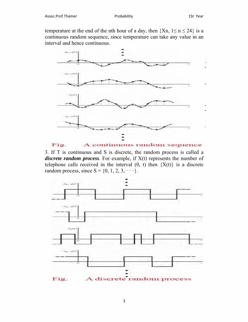
temperature at the end of the nth hour of a day, then {Xn, 1≤ n ≤ 24} is a continuous random sequence, since temperature can take any value in an interval and hence continuous.

3. If T is continuous and S is discrete, the random process is called a discrete random process. For example, if X(t) represents the number of telephone calls received in the interval (0, t) then {X(t)} is a discrete random process, since S = {0, 1, 2, 3, · · ·}.


4

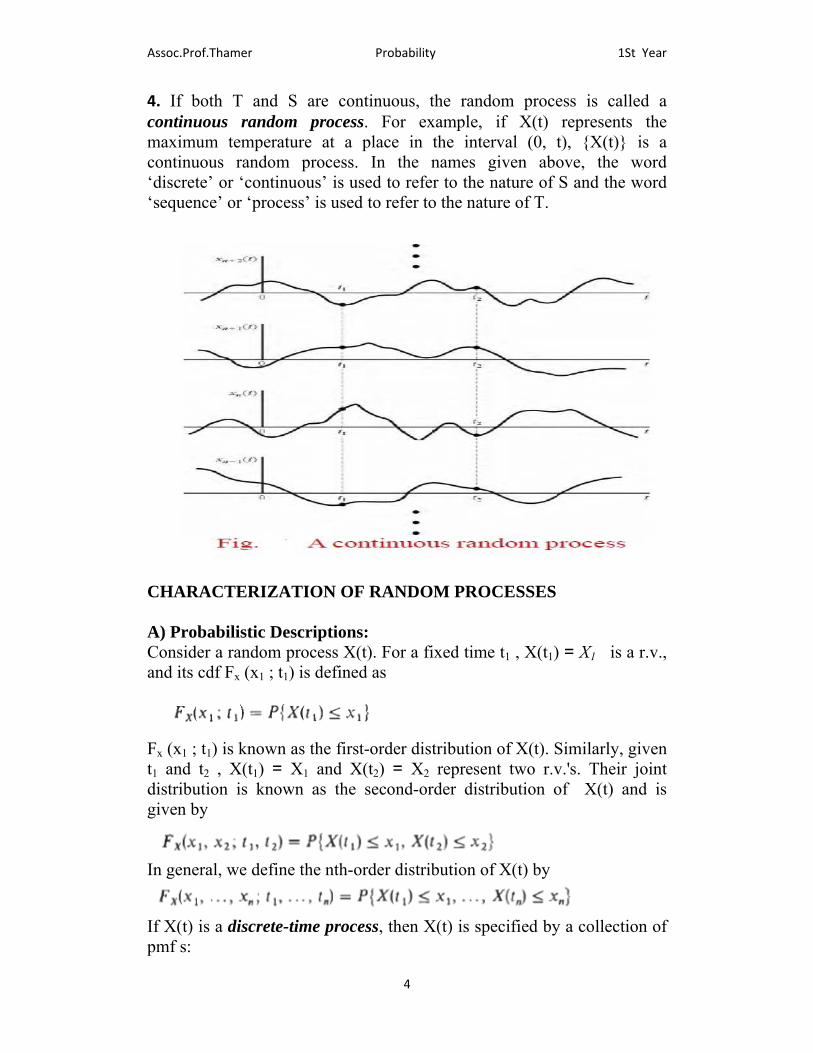
4. If both T and S are continuous, the random process is called a continuous random process. For example, if X(t) represents the maximum temperature at a place in the interval (0, t), {X(t)} is a continuous random process. In the names given above, the word ‘discrete’ or ‘continuous’ is used to refer to the nature of S and the word ‘sequence’ or ‘process’ is used to refer to the nature of T.

CHARACTERIZATION OF RANDOM PROCESSES A) Probabilistic Descriptions: Consider a random process X(t). For a fixed time t1 , X(t1) = X1 is a r.v., and its cdf Fx (x1 ; t1) is defined as

Fx (x1 ; t1) is known as the first-order distribution of X(t). Similarly, given t1 and t2 , X(t1) = X1 and X(t2) = X2 represent two r.v.'s. Their joint distribution is known as the second-order distribution of X(t) and is given by

In general, we define the nth-order distribution of X(t) by

If X(t) is a discrete-time process, then X(t) is specified by a collection of pmf s:


5

If X(t) is a continuous-time process, then X(t) is specified by a collection of pdf s:

B) Mean, Correlation, and Covariance Functions: As in the case of r.v.'s, random processes are often described by using statistical averages. The mean of X(t) is defined by

where X(t) is treated as a random variable for a fixed value of t. In general, µx(t) is a function of time, and it is often called the ensemble average of X(t). A measure of dependence among the r.v.'s of X(t) is provided by its autocorrelation function, defined by

Note that

The auto covariance function of X(t) is defined by

It is clear that if the mean of X(t) is zero, then Kx (t, s) = Rx (t, s). Note that the variance of X(t) is given by

C ) CLASSIFICATION OF RANDOM PROCESSES C.1 : Stationary Processes: A random process {X(t), t∈ T) is said to be stationary or strict-sense stationary if, for all n and for every set of time instants (t1 ∈ T, i = 1,2, . . . , n),


6

for any . Hence, the distribution of a stationary process will be unaffected by a shift in the time origin, and X(t) and X(t + ) will have the same distributions for any . Thus, for the first-order distribution,

where µ and are constants. Similarly, for the second-order distribution,

A consequences of the above condition is that the autocorrelation function of a second-order stationary process is a function only of time difference and not absolute time:

C.2: Wide-Sense Stationary Processes : If stationary condition of a random process X(t) does not hold for all n but holds for n ≤ k, then we say that the process X(t) is stationary to order k. If X(t) is stationary to order 2, then X(t) is said to be wide-sense stationary (WSS) or weak stationary. If X(t) is a WSS random process, then we have

or the second condition can be written as:-


7

C.3: Independent Processes: In a random process X(t), if X(ti) for i = 1,2, . . . , n are independent r.v.'s, so that for n = 2,3, . . . ,

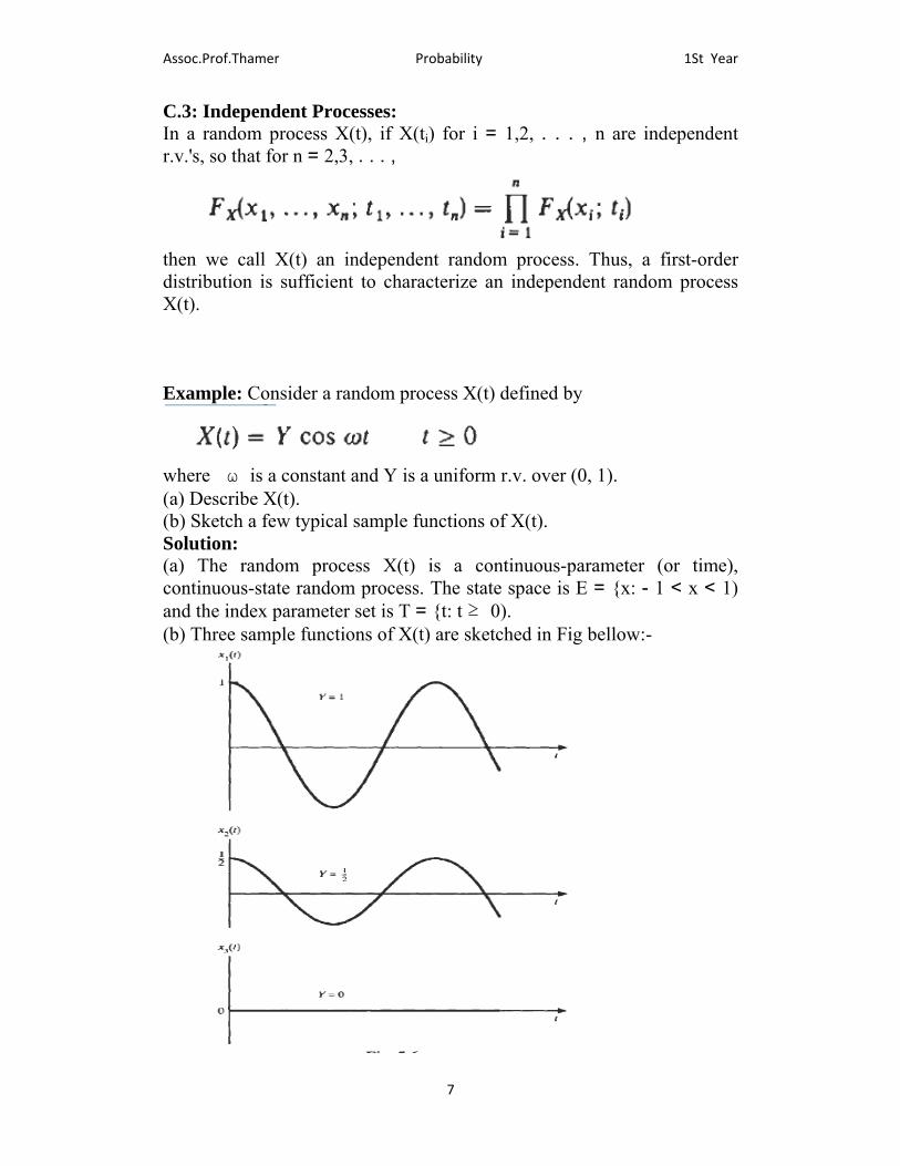
then we call X(t) an independent random process. Thus, a first-order distribution is sufficient to characterize an independent random process X(t). Example: Consider a random process X(t) defined by

where ω is a constant and Y is a uniform r.v. over (0, 1). (a) Describe X(t). (b) Sketch a few typical sample functions of X(t). Solution: (a) The random process X(t) is a continuous-parameter (or time), continuous-state random process. The state space is E = {x: - 1 < x < 1) and the index parameter set is T = {t: t ≥ 0). (b) Three sample functions of X(t) are sketched in Fig bellow:-


8

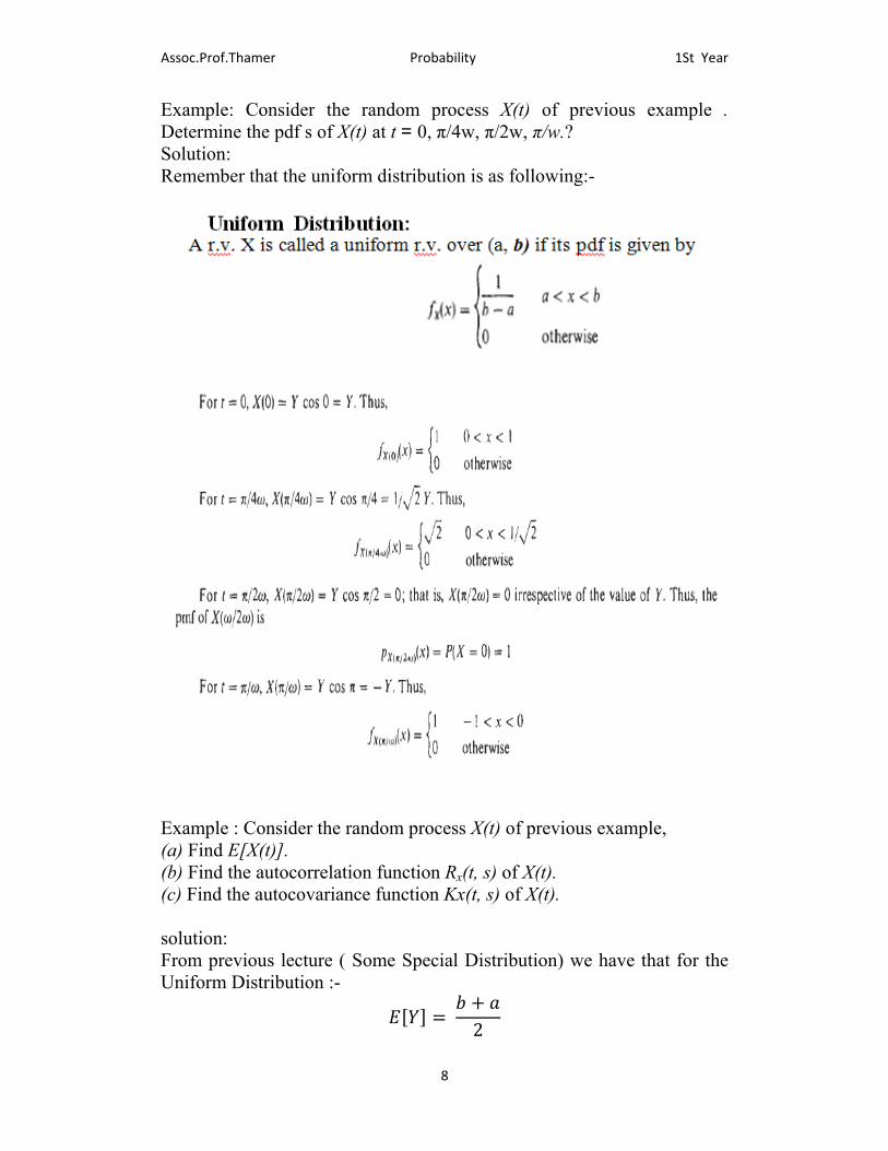
Example: Consider the random process X(t) of previous example . Determine the pdf s of X(t) at t = 0, π/4w, π/2w, π/w.? Solution: Remember that the uniform distribution is as following:-

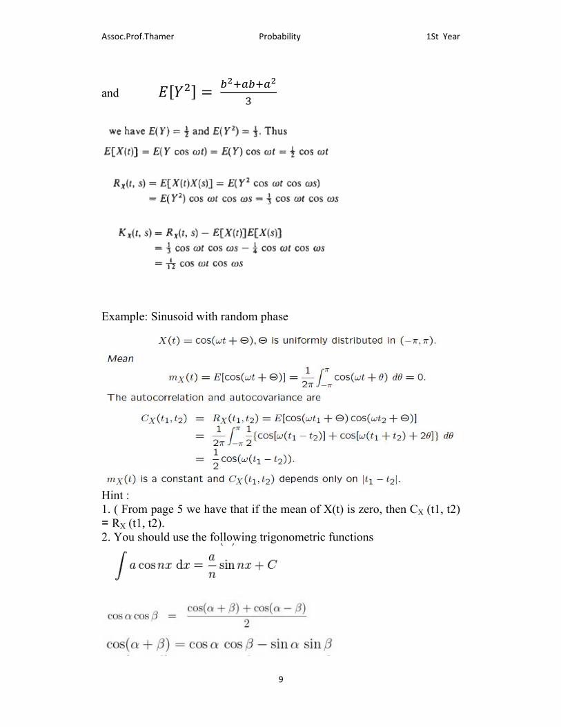
Example : Consider the random process X(t) of previous example, (a) Find E[X(t)]. (b) Find the autocorrelation function Rx(t, s) of X(t). (c) Find the autocovariance function Kx(t, s) of X(t). solution: From previous lecture ( Some Special Distribution) we have that for the Uniform Distribution :-

2


9

and

Example: Sinusoid with random phase

Hint : 1. ( From page 5 we have that if the mean of X(t) is zero, then CX (t1, t2) = RX (t1, t2). 2. You should use the following trigonometric functions


10

Example: A discrete-time random process is defined by Xn = sn, for n ≥ 0, where s is selected at random from the interval (0, 1). Find the mean

and autovariance functions of Xn? Solution:

Example: Show that the random process

is wide-sense stationary if A and are constants and Θ is a uniformly distributed random variable on the interval (0,2π). Solution:


11

Correlation Functions The autocorrelation of a random process X(t) is given by

If X(t) is at least wide-sense stationary then


12

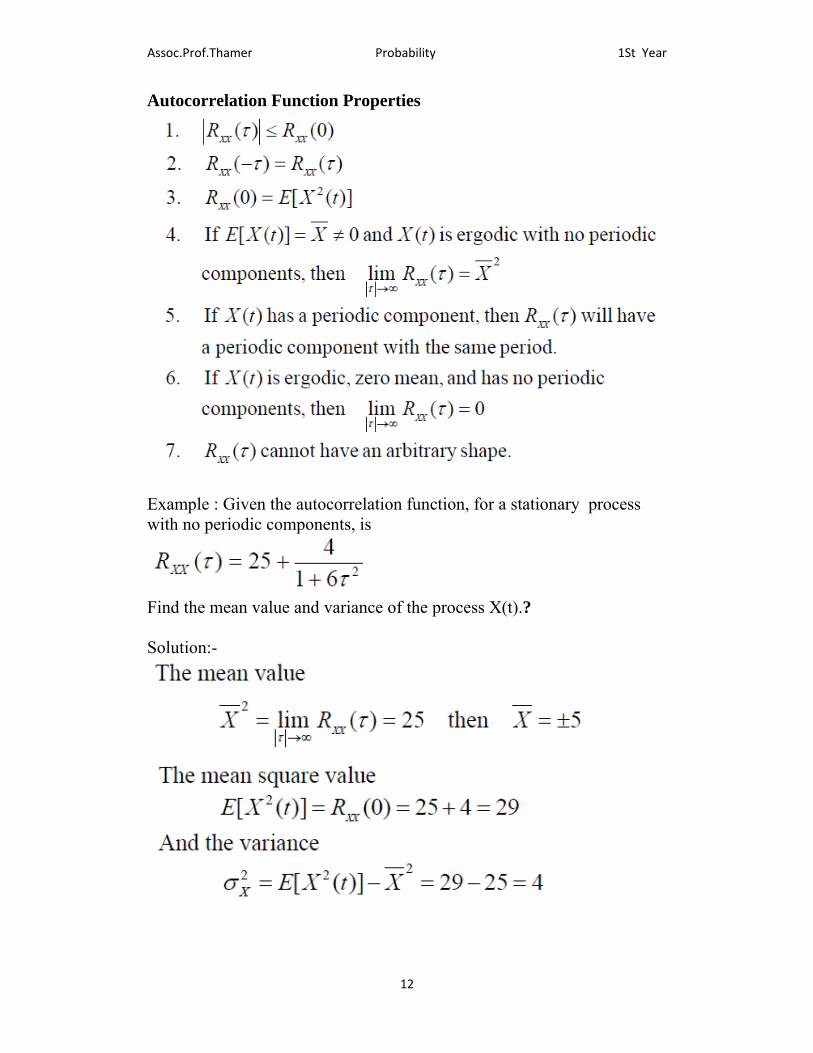
Autocorrelation Function Properties

Example : Given the autocorrelation function, for a stationary process with no periodic components, is

Find the mean value and variance of the process X(t).? Solution:-


13

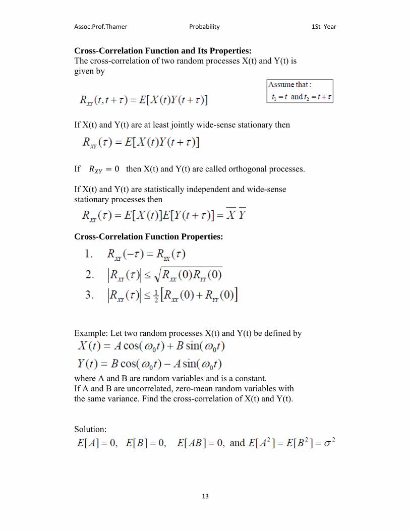
Cross-Correlation Function and Its Properties: The cross-correlation of two random processes X(t) and Y(t) is given by

If X(t) and Y(t) are at least jointly wide-sense stationary then

If 0 then X(t) and Y(t) are called orthogonal processes. If X(t) and Y(t) are statistically independent and wide-sense stationary processes then

Cross-Correlation Function Properties:

Example: Let two random processes X(t) and Y(t) be defined by

where A and B are random variables and is a constant. If A and B are uncorrelated, zero-mean random variables with the same variance. Find the cross-correlation of X(t) and Y(t). Solution:


14

Hint:


1

Spectral Characteristics of Random Processes In the study of deterministic signals and systems, frequency domain techniques (e.g., Fourier transform) provide a valuable tool that allows the engineer to gain significant insights into a variety of problems. In this lecture, we develop frequency domain tools for studying random processes. For a deterministic continuous signal, x(t ), the Fourier transform is used to describe its spectral content. In this text, we write the Fourier transform pair as:-

then | | represents its energy spectrum. This follows from Parseval’s theorem ( Parseval: Energy in time-domain=energy in frequency domain ) since the signal energy is given by


2

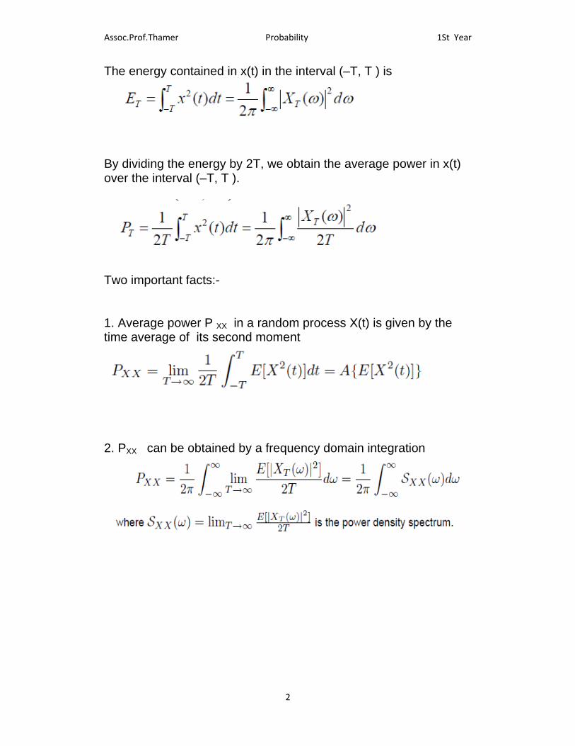
The energy contained in x(t) in the interval (–T, T ) is

By dividing the energy by 2T, we obtain the average power in x(t) over the interval (–T, T ).

Two important facts:- 1. Average power P XX in a random process X(t) is given by the time average of its second moment

2. PXX can be obtained by a frequency domain integration


3

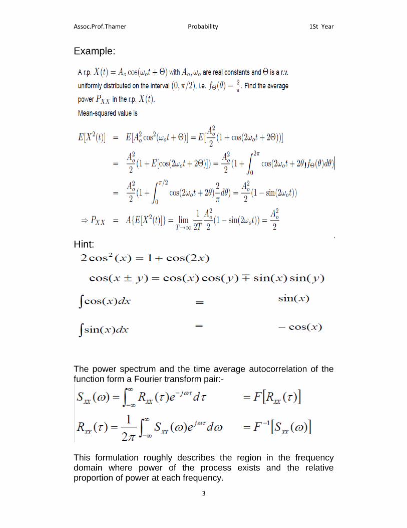
Example:

Hint:

The power spectrum and the time average autocorrelation of the function form a Fourier transform pair:-

This formulation roughly describes the region in the frequency domain where power of the process exists and the relative proportion of power at each frequency.


4

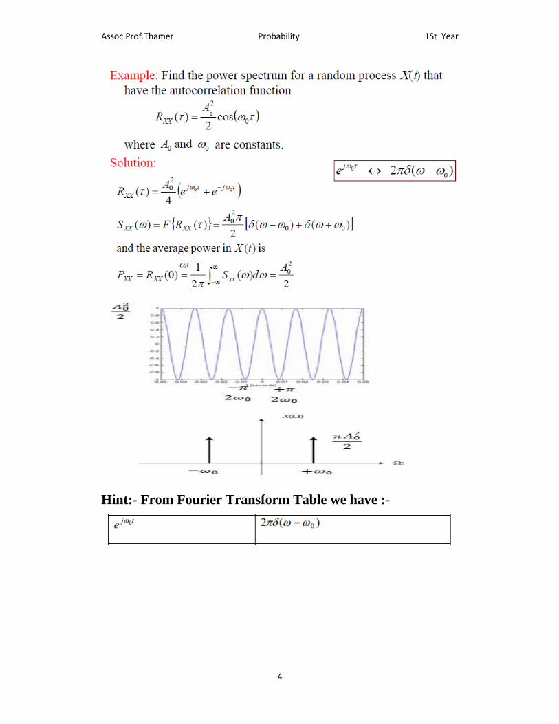
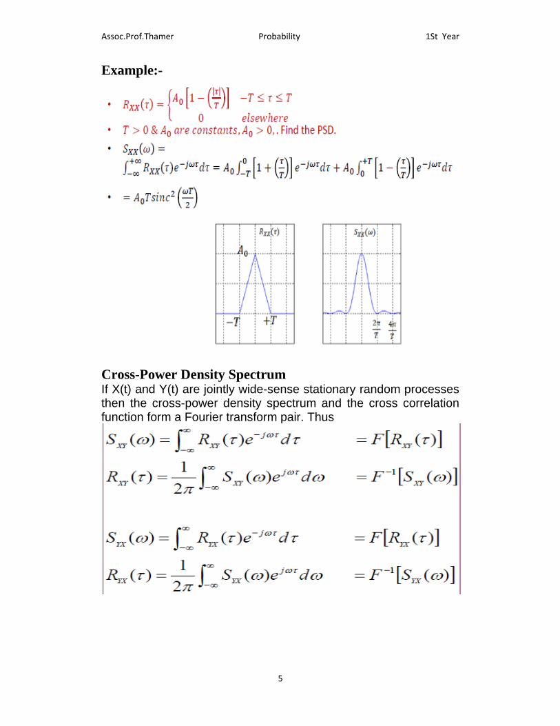
Hint:- From Fourier Transform Table we have :-


5

Example:-

Cross-Power Density Spectrum If X(t) and Y(t) are jointly wide-sense stationary random processes then the cross-power density spectrum and the cross correlation function form a Fourier transform pair. Thus


6

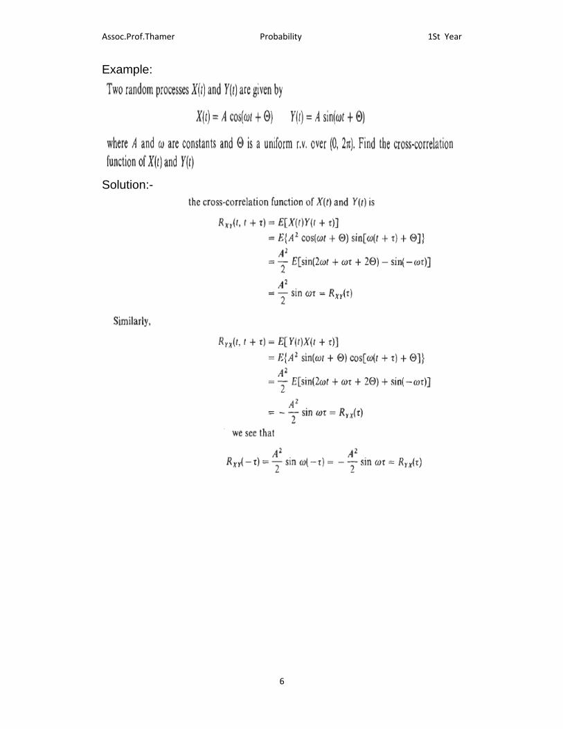
Example:

Solution:-


7

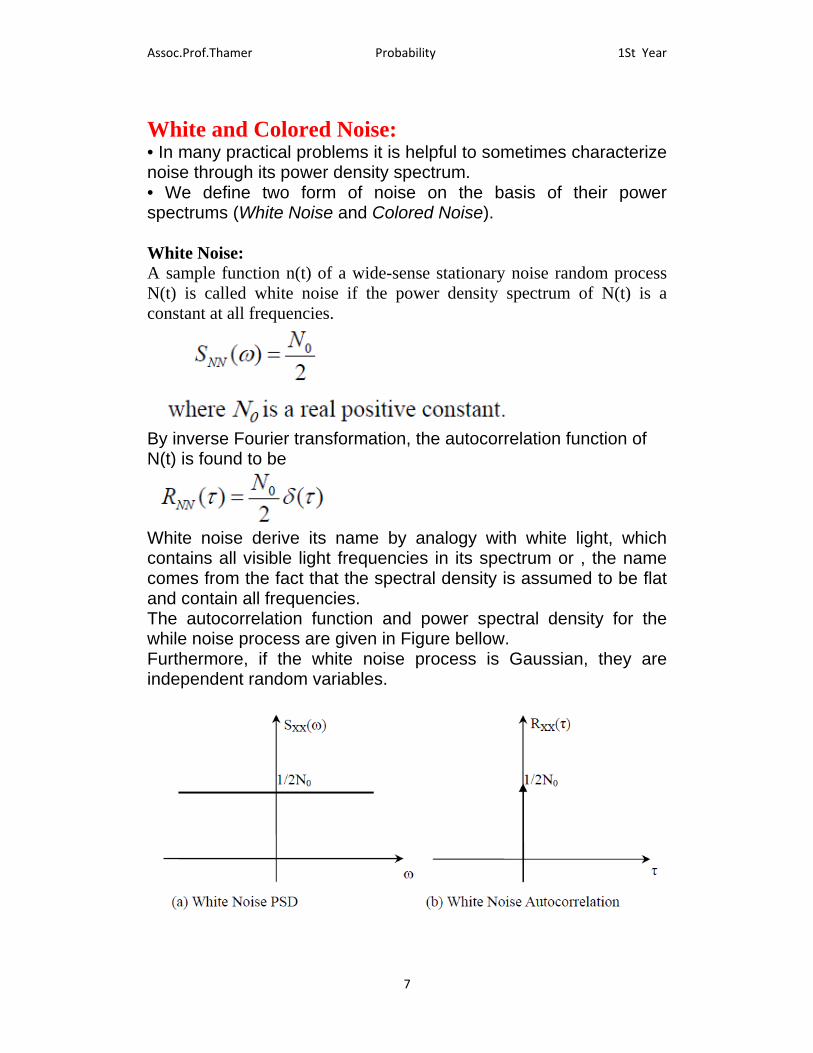
White and Colored Noise: • In many practical problems it is helpful to sometimes characterize noise through its power density spectrum. • We define two form of noise on the basis of their power spectrums (White Noise and Colored Noise). White Noise: A sample function n(t) of a wide-sense stationary noise random process N(t) is called white noise if the power density spectrum of N(t) is a constant at all frequencies.

By inverse Fourier transformation, the autocorrelation function of N(t) is found to be

White noise derive its name by analogy with white light, which contains all visible light frequencies in its spectrum or , the name comes from the fact that the spectral density is assumed to be flat and contain all frequencies. The autocorrelation function and power spectral density for the while noise process are given in Figure bellow. Furthermore, if the white noise process is Gaussian, they are independent random variables.


8

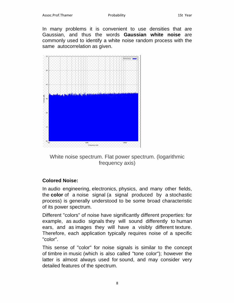
In many problems it is convenient to use densities that are Gaussian, and thus the words Gaussian white noise are commonly used to identify a white noise random process with the same autocorrelation as given.

White noise spectrum. Flat power spectrum. (logarithmic frequency axis)

Colored Noise:

In audio engineering, electronics, physics, and many other fields, the color of a noise signal (a signal produced by a stochastic process) is generally understood to be some broad characteristic of its power spectrum.

Different "colors" of noise have significantly different properties: for example, as audio signals they will sound differently to human ears, and as images they will have a visibly different texture. Therefore, each application typically requires noise of a specific "color".

This sense of "color" for noise signals is similar to the concept of timbre in music (which is also called "tone color"); however the latter is almost always used for sound, and may consider very detailed features of the spectrum.


9

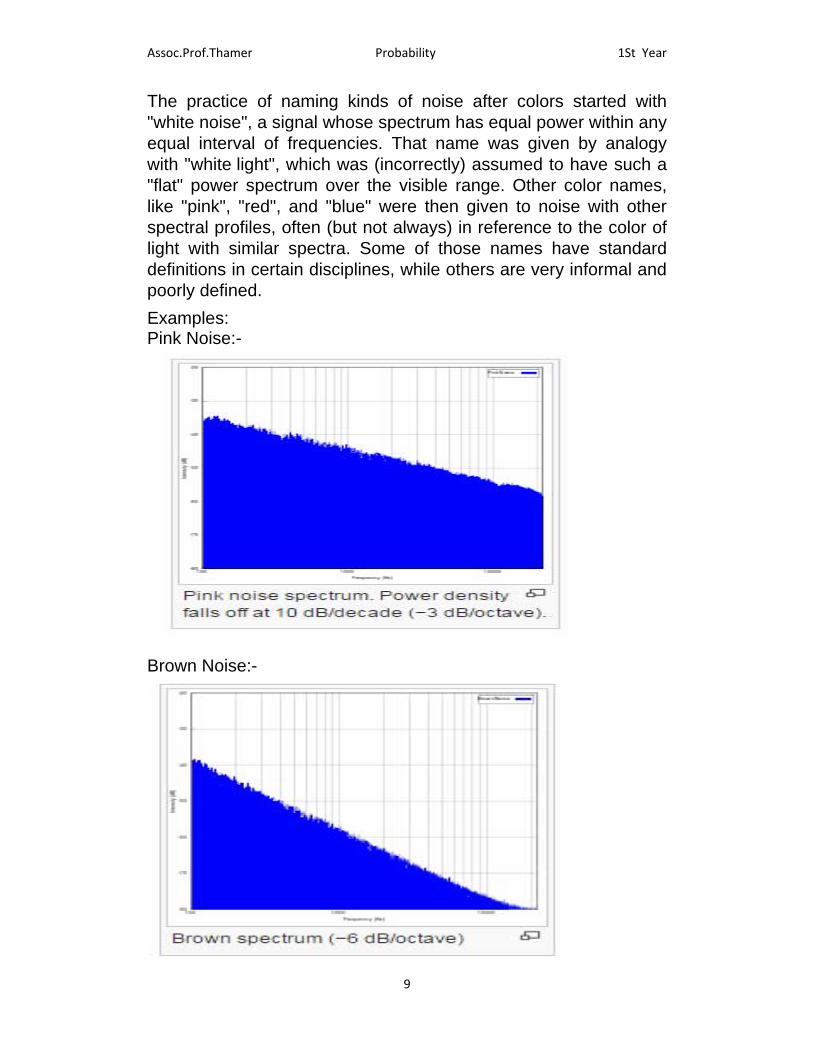
The practice of naming kinds of noise after colors started with "white noise", a signal whose spectrum has equal power within any equal interval of frequencies. That name was given by analogy with "white light", which was (incorrectly) assumed to have such a "flat" power spectrum over the visible range. Other color names, like "pink", "red", and "blue" were then given to noise with other spectral profiles, often (but not always) in reference to the color of light with similar spectra. Some of those names have standard definitions in certain disciplines, while others are very informal and poorly defined.

Examples: Pink Noise:-

Brown Noise:-


10

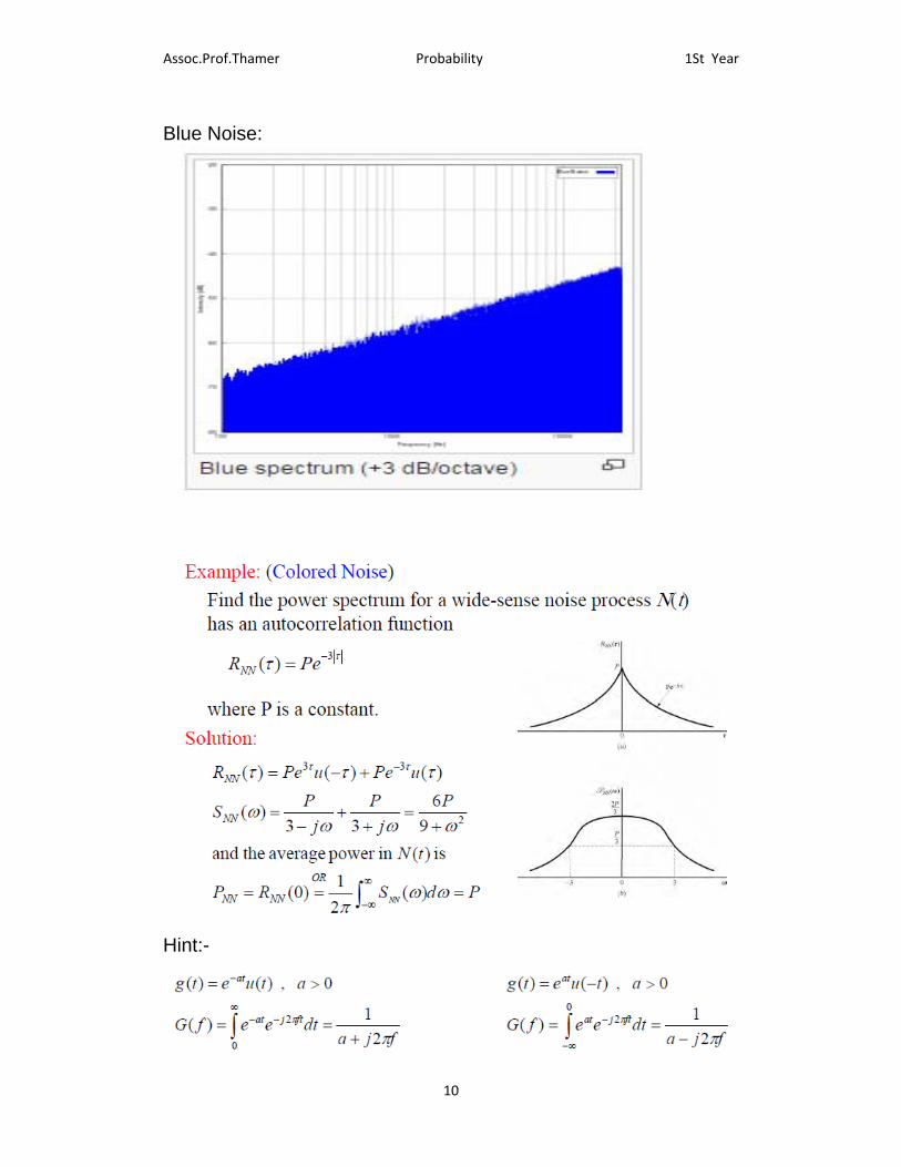
Blue Noise:

Hint:-


11

where a = 3 and x =w then 12

∗6

9 12

∗ 6 1

3

12

6 ∗ 13tan

3

Random Process (or Stochastic Process)

Documents

Transcript of Random Process (or Stochastic Process)