Quantitative stability of fully random mixed-integer two-stage stochastic programs

Optimization Letters (2008) 2:377–388DOI 10.1007/s11590-007-0066-1

ORIGINAL PAPER

Quantitative stability of fully random mixed-integertwo-stage stochastic programs

W. Römisch · S. Vigerske

Received: 8 January 2007 / Accepted: 13 August 2007 / Published online: 19 September 2007© Springer-Verlag 2007

Abstract Mixed-integer two-stage stochastic programs with fixed recourse matrix,random recourse costs, technology matrix, and right-hand sides are considered. Quan-titative continuity properties of its optimal value and solution set are derived whenthe underlying probability distribution is perturbed with respect to an appropriateprobability metric.

Keywords Stochastic programming · Two-stage · Mixed-integer · Stability · Weakconvergence · Probability metric · Discrepancy

1 Introduction

Mixed-integer two-stage stochastic programs model a variety of practical decisionproblems under stochastic uncertainty, e.g., in chemical engineering, power produc-tion, and trading planning [8,13,14]. The probability distribution of the stochasticprogramming model reflects the available knowledge on the randomness at the mod-eling stage. When solving such stochastic programming models, the probability dis-tribution is approximately replaced in most cases by a discrete probability measurewith finite support. Hence, perturbing or approximating the probability distributionof such models is an important issue for modeling, theory, and numerical methods instochastic integer programming. While much is known on the structure and algorithmsof/for mixed-integer two-stage stochastic programs (cf. the surveys [11,12,21,22]),the available (quantitative) stability or statistical estimation results do not cover situ-ations with stochastic costs (or prices) (cf. [7,18,19]).

W. Römisch (B) · S. VigerskeInstitute of Mathematics, Humboldt-University Berlin, 10099 Berlin, Germanye-mail: [email protected]

123

378 W. Römisch, S. Vigerske

Mixed-integer two-stage stochastic programs are of the form

min

⎧⎨

⎩

∫

Ξ

f0(x, ξ)d P(ξ) : x ∈ X

⎫⎬

⎭, (1)

where the (first-stage) feasible set X ⊆ Rm is closed, Ξ is a closed subset of R

s ,the function f0 from R

m × Ξ to the extended reals R is a random lower semicon-tinuous function, and P belongs to the set of all Borel probability measures P(Ξ)on Ξ . Recall that f0 is a random lower semicontinuous function if its epigraphicalmapping ξ �→ epi f0(·, ξ) := {(x, r) ∈ R

m × R : f0(x, ξ) ≤ r} is closed-valued andmeasurable. In mixed-integer two-stage stochastic programs, f0 is of the form

f0(x, ξ) = 〈c, x〉 +Φ(q(ξ), h(ξ)− T (ξ)x) ((x, ξ) ∈ Rm ×Ξ), (2)

whereΦ(u, t) denotes the optimal value of the (second-stage) mixed-integer program(with cost u and right-hand side t), and q(ξ), T (ξ), and h(ξ) are the stochastic cost,technology matrix, and right-hand side, respectively.

With v(P) and S(P) denoting the optimal value and solution set of (1), respectively,the quantitative stability results for stochastic programs developed in [18] (see [18,Theorems 5 and 9]) imply, in particular, the estimates

|v(P)− v(Q)| ≤ L supx∈X

∣∣∣∣∣∣

∫

Ξ

f0(x, ξ)(P − Q)(dξ)

∣∣∣∣∣∣

(3)

∅ = S(Q) ⊆ S(P)+ ΨP

⎛

⎝L supx∈X

∣∣∣∣∣∣

∫

Ξ

f0(x, ξ)(P − Q)(dξ)

∣∣∣∣∣∣

⎞

⎠ , (4)

where L > 0 is some constant, X is assumed to be compact, ΨP is the conditioningfunction, and P and Q belong to a suitable subset of P(Ξ). The function ΨP dependson the growth behavior of the objective function near the solution set and is specifiedin (11) of Sect. 3.

The aim of this paper is to extend the quantitative continuity properties of v(·) andS(·) in [16,20] to cover situations with stochastic costs. To this end, we need quanti-tative continuity and growth properties of optimal value functions and solution sets ofparametric mixed-integer linear programs. Such properties are known for parametricright-hand sides [4,5,20] and parametric costs separately [1,2,6]. Since to our knowl-edge simultaneous perturbation results with respect to right-hand sides and costs areless familiar, we discuss such properties of optimal value functions in Proposition 1.These results are then used in Sect. 3 to obtain the desired quantitative stability result(Theorem 1) for fully random mixed-integer two-stage stochastic programs with fixedrecourse. The relevant probability metric (9) on subsets of P(Ξ) and its relations toFortet–Mourier metrics and polyhedral discrepancies are also discussed (Remark 1).The latter metrics may be used for designing moderately sized discrete approximationsto P by optimal scenario reduction of discrete probability measures [9,10].

123

Quantitative stability of mixed-integer two-stage stochastic programs 379

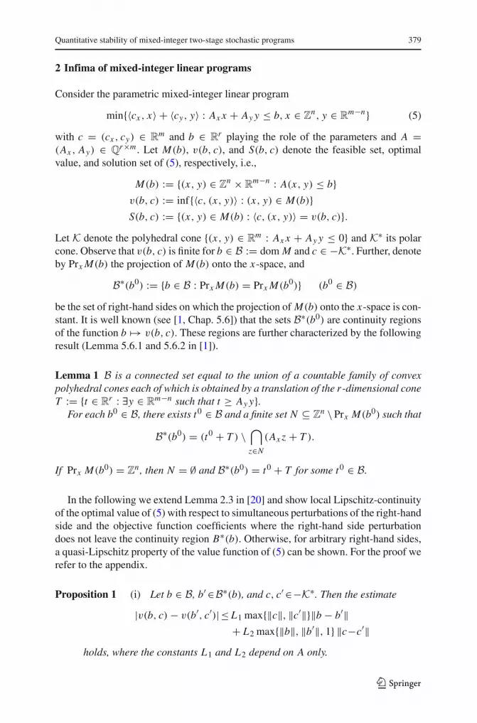
2 Infima of mixed-integer linear programs

Consider the parametric mixed-integer linear program

min{〈cx , x〉 + 〈cy, y〉 : Ax x + Ay y ≤ b, x ∈ Zn, y ∈ R

m−n} (5)

with c = (cx , cy) ∈ Rm and b ∈ R

r playing the role of the parameters and A =(Ax , Ay) ∈ Q

r×m . Let M(b), v(b, c), and S(b, c) denote the feasible set, optimalvalue, and solution set of (5), respectively, i.e.,

M(b) := {(x, y) ∈ Zn × R

m−n : A(x, y) ≤ b}v(b, c) := inf{〈c, (x, y)〉 : (x, y) ∈ M(b)}S(b, c) := {(x, y) ∈ M(b) : 〈c, (x, y)〉 = v(b, c)}.

Let K denote the polyhedral cone {(x, y) ∈ Rm : Ax x + Ay y ≤ 0} and K∗ its polar

cone. Observe that v(b, c) is finite for b ∈ B := dom M and c ∈ −K∗. Further, denoteby Prx M(b) the projection of M(b) onto the x-space, and

B∗(b0) := {b ∈ B : Prx M(b) = Prx M(b0)} (b0 ∈ B)

be the set of right-hand sides on which the projection of M(b) onto the x-space is con-stant. It is well known (see [1, Chap. 5.6]) that the sets B∗(b0) are continuity regionsof the function b �→ v(b, c). These regions are further characterized by the followingresult (Lemma 5.6.1 and 5.6.2 in [1]).

Lemma 1 B is a connected set equal to the union of a countable family of convexpolyhedral cones each of which is obtained by a translation of the r-dimensional coneT := {t ∈ R

r : ∃y ∈ Rm−n such that t ≥ Ay y}.

For each b0 ∈ B, there exists t0 ∈ B and a finite set N ⊆ Zn \ Prx M(b0) such that

B∗(b0) = (t0 + T ) \⋂

z∈N

(Ax z + T ).

If Prx M(b0) = Zn, then N = ∅ and B∗(b0) = t0 + T for some t0 ∈ B.

In the following we extend Lemma 2.3 in [20] and show local Lipschitz-continuityof the optimal value of (5) with respect to simultaneous perturbations of the right-handside and the objective function coefficients where the right-hand side perturbationdoes not leave the continuity region B∗(b). Otherwise, for arbitrary right-hand sides,a quasi-Lipschitz property of the value function of (5) can be shown. For the proof werefer to the appendix.

Proposition 1 (i) Let b ∈ B, b′ ∈B∗(b), and c, c′ ∈−K∗. Then the estimate

|v(b, c)− v(b′, c′)|≤ L1 max{‖c‖, ‖c′‖}‖b − b′‖+ L2 max{‖b‖, ‖b′‖, 1} ‖c−c′‖

holds, where the constants L1 and L2 depend on A only.

123


(ii) Let b, b′ ∈ B and c, c′ ∈ −K∗. Then we have

|v(b, c)− v(b′, c′)| ≤ max{‖c‖, ‖c′‖}(L‖b − b′‖ + 2�)

+L max{‖b‖, ‖b′‖}‖c − c′‖,

where the constants L and � depend on A only.

The following result is [4, Theorem 2.1] and can be found in similar form also in[2]. Together with Proposition 1 it is needed to prove Lemma 3.

Lemma 2 Let c ∈ −K∗. The mapping b �→ S(b, c) is quasi-Lipschitz continuous onB with constants L1 and L2 not depending on b and c, i.e.,

dH (S(b, c), S(b′, c)) ≤ L1‖b − b′‖ + L2,

where dH denotes the Hausdorff distance on subsets of Rm.

3 Quantitative stability of mixed-integer two-stage stochastic programs

Let us consider the stochastic program

min

⎧⎨

⎩〈c, x〉 +

∫

Ξ

Φ(q(ξ), h(ξ)− T (ξ)x)P(dξ) : x ∈ X

⎫⎬

⎭, (6)

where Φ is the infimum function of a mixed-integer linear program given by

Φ(u, t) := inf{〈u1, y〉 + 〈u2, y〉 : W y + W y ≤ t, y ∈ Z

m, y ∈ Rm}

(7)

for all pairs (u, t) ∈ Rm+m × R

r , and c ∈ Rm , X is a closed subset of R

m , Ξ a poly-hedron in R

s , W and W are (r, m)- and (r, m)-matrices, respectively, q(ξ) ∈ Rm+m ,

h(ξ) ∈ Rr , and the (r,m)-matrix T (ξ) are affine functions of ξ ∈ R

s , and P ∈ P(Ξ).We need the following conditions to have the model (6) well defined:

(B1) The matrices W and W have only rational elements.(B2) For each pair (x, ξ) ∈ X ×Ξ it holds that h(ξ)− T (ξ)x ∈ T , where

T :={

t ∈ Rr : ∃(y, y) ∈ Z

m × Rm such that W y + W y ≤ t

}.

(B3) For each ξ ∈ Ξ the recourse cost q(ξ) belongs to the dual feasible set

U :={

u = (u1, u2) ∈ Rm+m : ∃z ∈ R

r− such that W �z = u1, W �z = u2

}.

(B4) P ∈ P2(Ξ), i.e., P ∈ P(Ξ) and∫

Ξ‖ξ‖2 P(dξ) < +∞.

123


The conditions (B2) and (B3) mean relatively complete recourse and dual feasibility,respectively. We note that (B2) and (B3) implyΦ(u, t) to be finite for all (u, t) ∈ U×T .The following additional properties of the value function Φ on U × T are importantin the context of this paper.

Lemma 3 Assume (B1)–(B3). Then there exists a countable partition of T into Borelsubsets Bi , i.e., T = ⋃

i∈NBi such that

(i) Bi = (bi + T ) \ ⋃N0j=1(bi, j + T ), where bi , bi, j ∈ R

r , i ∈ N, j = 1, . . . , N0,N0 ∈ N does not depend on i , and T := {t ∈ R

r : ∃y ≥ 0 such that t ≥ W y}.Moreover there exists an N1 ∈ N such that for all t ∈ T the ball B(t, 1) in R

r isintersected by at most N1 different subsets Bi .

(ii) the restriction Φ∣∣∣U×B′

i, where B′

i := Bi ∩ {h(ξ)− T (ξ)x |(x, ξ) ∈ X ×Ξ}, has

the property that there exists a constant L > 0 independent of i , s.t.

|Φ(u, t)−Φ(u, t)|≤ L(max{1, ‖t‖, ‖t‖}‖u − u‖+max{1, ‖u‖, ‖u‖}‖t− t‖).

Furthermore, the function Φ is lower semicontinuous and piecewise polyhedral onU ×T and there exist constants D, d > 0 such that it holds for all pairs (u, t), (u, t) ∈U × T :

|Φ(u, t)−Φ(u, t)|≤ D(max{1, ‖t‖, ‖t‖}(‖u−u‖+d)+max{1, ‖u‖, ‖u‖}‖t − t‖).

The first part of (i) is Lemma 1. The second part is an extension of [20, Lemma 2.5]to the function Φ(u, t) since the relevant constants in its proof do not depend on theobjective function as recalled in Lemma 2. Part (ii) and the quasi-Lipschitz propertyof Φ is Proposition 1.

The representation of Φ is given on countably many (possibly unbounded) Borelsets. This requires to incorporate the tail behavior of P and leads to the followingrepresentation of the function f0.

Proposition 2 Assume (B1)–(B3) and X be bounded. For each R ≥ 1 and x ∈ X thereexist disjoint Borel subsets Ξ R

j,x of Ξ , j = 1, . . . , ν, whose closures are polyhedrawith a uniformly bounded number of faces such that

f0(x, ξ) =ν∑

j=0

(〈c, x〉 +Φ(q(ξ), h(ξ)− T (ξ)x))1Ξ Rj,x(ξ) ((x, ξ) ∈ X ×Ξ)

is Lipschitz continuous with respect to ξ on eachΞ Rj,x , j = 1, . . . , ν, with some uniform

Lipschitz constant. Here,Ξ R0,x := Ξ\∪νj=1Ξ

Rj,x is contained in {ξ ∈ R

s : ‖ξ‖∞ > R},ν is bounded by a multiple of Rr and 1A denotes the characteristic function of a set A.

Proof Since q(·), h(·) and T (·) are affine linear functions and X is bounded, thereexists a constant C > 0 such that the estimate

max{‖q(ξ)‖∞, ‖h(ξ)− T (ξ)x‖∞} ≤ C max{1, ‖ξ‖∞} (8)

123


holds for each pair in X × Ξ . Let R ≥ 1 and TR := T ∩ C RB∞, where B∞ is theunit ball w.r.t. the maximum norm ‖ · ‖∞. As in [18, Proposition 34] there exist anumber ν ∈ N and disjoint Borel subsets {B j }νj=1 of C RB∞ such that their closuresare polyhedra and their union contains TR . Furthermore, when arguing as in the proofof [20, Proposition 3.1], ν is bounded above by κRr , where the constant κ > 0 isindependent of R. Now, let x ∈ X and consider the following disjoint Borel subsetsof Ξ :

Ξ Rj,x := {ξ ∈ Ξ : h(ξ)− T (ξ)x ∈ B j , ‖ξ‖∞ ≤ R} ( j = 1, . . . , ν),

Ξ R0,x := Ξ \

ν⋃

j=1

Ξ Rj,x ⊆ {ξ ∈ Ξ : ‖ξ‖∞ > R}.

Let x ∈ X and ξ, ξ ′ ∈ Ξ Rj,x for some j ∈ {1, . . . , ν}. By Lemma 3 we obtain

| f0(x, ξ)− f0(x, ξ′)| = |Φ(q(ξ), h(ξ)− T (ξ)x)−Φ(q(ξ ′), h(ξ ′)− T (ξ ′)x)|

≤ L(max{1, ‖q(ξ)‖∞, ‖q(ξ ′)‖∞}(‖h(ξ)− h(ξ ′)‖∞+‖(T (ξ)− T (ξ ′))x‖∞)+ max{1, ‖h(ξ)− T (ξ)x‖∞,‖h(ξ ′)− T (ξ ′)x‖∞}‖q(ξ)− q(ξ ′)‖∞)

≤ LC R(‖h(ξ)− h(ξ ′)‖∞ + ‖(T (ξ)− T (ξ ′))x‖∞+‖q(ξ)− q(ξ ′)‖∞)

≤ L1 R‖ξ − ξ ′‖∞,

where we used (8) for ξ, ξ ′ ∈ Ξ Rj,x , affine linearity of q(·), h(·), and T (·), and bound-

edness of X . We note that the constant L1 is independ of R. ��In order to state quantitative stability results for model (6) and inspired by the

estimates (3) and (4), we need a distance of probability measures that captures thebehavior of f0(x, ·) (x ∈ X ) in its continuity regions and the shape of these regions,respectively. This leads us to the following probability metric on P2(Ξ) for somek ∈ N:

ζ2,phk(P, Q) :=sup

⎧⎨

⎩

∣∣∣∣∣∣

∫

B

f (ξ)(P − Q)(dξ)

∣∣∣∣∣∣: f ∈ F2(Ξ), B ∈ Bphk

(Ξ)

⎫⎬

⎭. (9)

Here, Bphk(Ξ) denotes the set of all polyhedra being subsets ofΞ and having at most

k faces. The set F2(Ξ) contains all functions f : Ξ → R such that

| f (ξ)| ≤ max{1, ‖ξ‖2} and | f (ξ)− f (ξ )| ≤ max{1, ‖ξ‖, ‖ξ‖}‖ξ − ξ‖

holds for all ξ, ξ ∈ Ξ . We note that, unfortunately, the growth condition on f ismissing in the description of the set of functions in [16,18].

123


Before stating the main result, we define the function φP on R+ characterizing thetail behavior of P by φP (0) = 0 and

φP (t) := infR≥1

⎧⎪⎨

⎪⎩Rr+1t +

∫

{ξ∈Ξ :‖ξ‖∞>R}‖ξ‖2∞ P(dξ)

⎫⎪⎬

⎪⎭(t > 0), (10)

and the conditioning function ΨP by

ΨP (η) := η + ψ−1P (2η) (η ∈ R+), (11)

where the growth function ψP on R+ is

ψP (τ ) := min

⎧⎨

⎩

∫

Ξ

f0(x, ξ)P(dξ)− v(P) : d(x, S(P)) ≥ τ, x ∈ X

⎫⎬

⎭(12)

with inverse ψ−1P (t) := sup{τ ∈ R+ : ψP (τ ) ≤ t}. The functions φP and ψP are

nondecreasing, ΨP is increasing and all functions vanish at 0. Furthermore, one hasψP (τ ) > 0 if τ > 0 and ΨP (η) ↘ 0 if η ↘ 0.

Theorem 1 Let the conditions (B1)–(B4) be satisfied and X be compact.Then there exist constants L > 0 and k ∈ N such that

|v(P)− v(Q)| ≤ LφP(ζ2,phk(P, Q)) (13)

∅ = S(Q) ⊆ S(P)+ ΨP (LφP (ζ2,phk(P, Q)))B,

for each Q ∈ P2(Ξ). If∫

Ξ‖ξ‖p P(dξ) < +∞ for some p > 2, the estimate φP (t) ≤

Ctp−2

p+r−1 holds for every t ≥ 0 and some constant C > 0.

Proof Since the functionΦ is lower semicontinuous on U ×T (Lemma 3), f0 is lowersemicontinuous on X ×Ξ and, hence, a random lower semicontinuous function [17,Example 14.31]. Using Lemma 3 we obtain the estimate

| f0(x, ξ)| ≤ ‖c‖‖x‖ + D[max{1, ‖h(ξ)‖ + ‖T (ξ)‖‖x‖}(‖q(ξ)‖ + d)

+ max{1, ‖q(ξ)‖}(‖h(ξ)‖ + ‖T (ξ)‖‖x‖)]≤ C1 max{1, ‖ξ‖2}

for each pair (x, ξ) ∈ X × Ξ and some constant C1. Hence, the objective function〈c, x〉 + ∫

ΞΦ(q(ξ), h(ξ) − T (ξ)x)Q(dξ) is finite (if Q ∈ P2(Ξ)) and lower semi-

continuous (due to Fatou’s lemma). Since X is compact, the solution set S(Q) isnonempty.

From Proposition 2 we know that, for each R ≥ 1 and x ∈ X , there exist Borelsubsets Ξ R

j,x , j = 1, . . . , ν, of Ξ such that the function f Rj,x (·) := f0(x, ·)1Ξ R

j,xis

123


Lipschitz continuous on Ξ Rj,x with constant L1 R. We extend each function f R

j,x (·)to the whole of Ξ by preserving the Lipschitz constant. Then we have 1

L1 R f Rj,x (·) ∈

F2(Ξ). Furthermore, Proposition 2 implies that the closures of Ξ Rj,x are contained in

Bphk(Ξ) for some k ∈ N, that the number ν is bounded above by κRr , where the

constant κ > 0 is independent on R, and that Ξ R0,x := Ξ \ ⋃ν

j=1ΞRj,x is a subset of

{ξ ∈ Ξ : ‖ξ‖∞ > R}. For each Q ∈ P2(Ξ) and x ∈ X we obtain

∣∣∣∣∣∣

∫

Ξ

f0(x, ξ)(P − Q)(dξ)

∣∣∣∣∣∣=

∣∣∣∣∣∣∣∣

ν∑

j=0

∫

Ξ Rj,x

f0(x, ξ)(P − Q)(dξ)

∣∣∣∣∣∣∣∣

≤ν∑

j=1

∣∣∣∣∣∣∣∣

∫

Ξ Rj,x

f Rj,x (ξ)(P − Q)(dξ)

∣∣∣∣∣∣∣∣

+ I Rx (P, Q)

≤ νL1 R supf ∈F2(Ξ)j=1,...,ν

∣∣∣∣∣∣

∫

Ξ

f (ξ)χΞ Rj,x(ξ)(P − Q)(dξ)

∣∣∣∣∣∣

+I Rx (P, Q),

where the last summand on the right-hand side is given by

I Rx (P, Q) :=

∣∣∣∣∣∣∣∣

∫

Ξ R0,x

f0(x, ξ)(P − Q)(dξ)

∣∣∣∣∣∣∣∣

.

Using ν ≤ κRr and arguing as in [18, Theorem 35] we continue

∣∣∣∣∣∣

∫

Ξ

f0(x, ξ)(P − Q)(dξ)

∣∣∣∣∣∣≤ κL1 Rr+1ζ2,phk

(P, Q)+ I Rx (P, Q).

For the term I Rx (P, Q) we use the estimate | f0(x, ξ)| ≤ C1‖ξ‖2 for any pair (x, ξ) ∈

X × {ξ ∈ Ξ : ‖ξ‖∞ > R} and the norming constant C2 such that ‖ξ‖ ≤ C2‖ξ‖∞holds for all ξ ∈ R

s . We get

I Rx (P, Q) ≤ C1C2

2

∫

{ξ∈Ξ :‖ξ‖∞>R}‖ξ‖2∞(P + Q)(dξ).

123


Since the set {ξ ∈ Ξ : ‖ξ‖∞ > R} can be covered by 2s intersections ofΞ with openhalfspaces (whose closures belong to Bphk

(Ξ)), we can estimate

∫

{ξ∈Ξ :‖ξ‖∞>R}‖ξ‖2∞Q(dξ) ≤ 2sζ2,phk

(P, Q)+∫

{ξ∈Ξ :‖ξ‖∞>R}‖ξ‖2∞ P(dξ).

Hence, combining the last three estimates we get

supx∈X

∣∣∣∣∣∣

∫

Ξ

f0(x, ξ)(P − Q)(dξ)

∣∣∣∣∣∣≤ (κL1 Rr+1 + C1C2

2 2s)ζ2,phk(P, Q)

+2C1C22

∫

{ξ∈Ξ :‖ξ‖>R}‖ξ‖2∞ P(dξ)

for any R ≥ 1. Taking the infimum with respect to R ≥ 1 we obtain

supx∈X

∣∣∣∣∣∣

∫

Ξ

f0(x, ξ)(P − Q)(dξ)

∣∣∣∣∣∣≤ CφP (ζ2,phk

(P, Q))

with some constant C > 0. Now, the result is a consequence of the estimates (3) and (4).If

∫

Ξ‖ξ‖pd P(ξ) < +∞ for some p > 2, it holds that

∫

{ξ∈Ξ :‖ξ‖∞>R} ‖ξ‖2∞d P(ξ) ≤R2−p

∫

Ξ‖ξ‖p∞ P(dξ) by Markov’s inequality. The desired estimate follows by insert-

ing R = t−1

p+r−1 for small t > 0 into the function whose infinum w.r.t. R ≥ 1 isφP (t):

φP (t) ≤ t−r+1

p+r−1 +1 + tp−2

p+r−1

∫

Ξ

‖ξ‖p∞ P(dξ) ≤ Ctp−2

p+r−1 .

��The boundedness condition on X may be relaxed if localized optimal values and

solution sets are considered (see [18]). In case that the underlying distribution P andits perturbations Q have supports in some bounded subsetΞ of R

s , the stability resultimproves slightly.

Corollary 1 Let the conditions (B1)–(B3) be satisfied, P ∈ P(Ξ), X and Ξ bebounded. Then there exist constants L > 0 and k ∈ N such that

|v(P)− v(Q)| ≤ Lζ2,phk(P, Q)

∅ = S(Q) ⊆ S(P)+ ΨP (Lζ2,phk(P, Q))B,

holds for each Q ∈ P(Ξ).

123


Proof Since Ξ is bounded, we have P2(Ξ) = P(Ξ). Moreover, the function φP (t)(see (10)) can be estimated by Rr+1t for some sufficiently large R > 0. Hence,Theorem 1 implies the assertion. ��

Remark 1 Since Ξ ∈ Bphk(Ξ) for some k ∈ N, we obtain from (9) by choosing

B := Ξ and f ≡ 1, respectively,

max{ζ2(P, Q), αphk(P, Q)} ≤ ζ2,phk

(P, Q) (14)

for all P, Q ∈ P2(Ξ). Here, ζ2 and αphkdenote the second order Fortet–Mourier

metric [15, Sect. 5.1] and the polyhedral discrepancy

ζ2(P, Q) := supf ∈F2(Ξ)

∣∣∣∣∣∣

∫

Ξ

f (ξ)P(dξ)−∫

Ξ

f (ξ)Q(dξ)

∣∣∣∣∣∣

αphk(P, Q) := sup

B∈Bphk (Ξ)

|P(B)− Q(B)|,

respectively. Hence, convergence with respect to ζ2,phkimplies weak convergence (see

[3]), convergence of second order absolute moments, and convergence with respectto the polyhedral discrepancy αphk

. For bounded Ξ ⊂ Rs the technique in the proof

of [20, Proposition 3.1] can be employed to obtain

ζ2,phk(P, Q) ≤ Csαphk

(P, Q)1

s+1 (P, Q ∈ P(Ξ)) (15)

for some constant Cs > 0. In view of (14), (15) the metric ζ2,phkis stronger than αphk

in general, but in case of bounded Ξ both distances metrize the same topology onP(Ξ).

For more specific models (6), improvements of the above results may be obtainedby exploiting specific recourse structures, i.e., by using additional information on theshape of the sets Bi in Lemma 3 and on the behavior of the (value) function Φ onthese sets. This may lead to stability results with respect to probability metrics that are(much) weaker than ζ2,phk

. For example, if q and T are fixed and h(·) is of the formh(ξ) := ξ (i.e., r = s), the closures of the Bi belong to a class of polyhedra which iscompletely characterized in [20, Sect. 3]. If, in addition, the model has pure integerrecourse, the stability result is valid with respect to the Kolmogorov metric

dK(P, Q) := supz∈Rs

|P((−∞, z])− Q((−∞, z])|

on P(Ξ) instead of ζ2,phkif Ξ is bounded (see also [20, Proposition 3.4]).

123


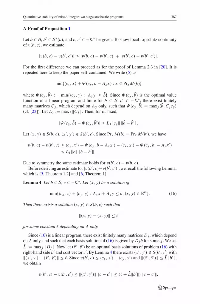
A Proof of Proposition 1

Let b ∈ B, b′ ∈ B∗(b), and c, c′ ∈ −K∗ be given. To show local Lipschitz continuityof v(b, c), we estimate

|v(b, c)− v(b′, c′)| ≤ |v(b, c)− v(b′, c)| + |v(b′, c)− v(b′, c′)|.

For the first difference we can proceed as for the proof of Lemma 2.3 in [20]. It isrepeated here to keep the paper self-contained. We write (5) as

min{〈cx , x〉 + Ψ (cy, b − Ax x) : x ∈ Prx M(b)}

where Ψ (cy, b) := min{〈cy, y〉 : Ay y ≤ b}. Since Ψ (cy, b) is the optimal valuefunction of a linear program and finite for b ∈ B, c′ ∈ −K∗, there exist finitelymany matrices C j , which depend on Ay only, such that Ψ (cy, b) = max j 〈b,C j cy〉(cf. [23]). Let L1 := max j ‖C j‖. Then, for cy fixed,

|Ψ (cy, b)− Ψ (cy, b′)| ≤ L1‖cy‖ ‖b − b′‖.

Let (x, y) ∈ S(b, c), (x ′, y′) ∈ S(b′, c). Since Prx M(b) = Prx M(b′), we have

v(b, c)− v(b′, c) ≤ 〈cx , x ′〉 + Ψ (cy, b − Ax x ′)− 〈cx , x ′〉 − Ψ (cy, b′ − Ax x ′)≤ L1‖c‖ ‖b − b′‖.

Due to symmetry the same estimate holds for v(b′, c)− v(b, c).Before deriving an estimate for |v(b′, c)−v(b′, c′)|, we recall the following Lemma,

which is [5, Theorem 1.2] and [6, Theorem 1].

Lemma 4 Let b ∈ B, c ∈ −K∗. Let (x, y) be a solution of

min{〈cx , x〉 + 〈cy, y〉 : Ax x + Ay y ≤ b, (x, y) ∈ Rm}. (16)

Then there exists a solution (x, y) ∈ S(b, c) such that

‖(x, y)− (x, y)‖ ≤ �

for some constant � depending on A only.

Since (16) is a linear program, there exist finitely many matrices D j , which dependon A only, and such that each basis solution of (16) is given by D j b for some j . We setL := max j ‖D j‖. Now let (x ′, y′) be an optimal basis solutions of problem (16) withright-hand side b′ and cost vector c′. By Lemma 4 there exists (x ′, y′) ∈ S(b′, c′)with‖(x ′, y′)− (x ′, y′)‖ ≤ �. Since v(b′, c) ≤ 〈cx , x ′〉 + 〈cy, y′〉 and ‖(x ′, y′)‖ ≤ L‖b′‖,we obtain

v(b′, c)− v(b′, c′) ≤ ‖(x ′, y′)‖ ‖c − c′‖ ≤ (�+ L‖b′‖) ‖c − c′‖.

123


Due to symmetry, a similar estimate holds for v(b′, c′)− v(b′, c). The second part ofProposition 1 follows from Lemma 4 and stability results for linear programs.

Acknowledgments This work was supported by the DFG Research Center Matheon in Berlin and theBMBF under the grant 03SF0312E. We thank an anonymous referee whose comments helped to improvean earlier version of this paper.

References

1. Bank, B., Guddat, J., Klatte, D., Kummer, B., Tammer, K.: Non-Linear Parametric Optimization.Akademie-Verlag, Berlin (1982)

2. Bank, B., Mandel, R.: Parametric Integer Optimization. Akademie-Verlag, Berlin (1988)3. Billingsley, P.: Convergence of Probability Measures. Wiley, New York (1968)4. Blair, C.E., Jeroslow, R.G.: The value function of a mixed integer program I. Discrete Math. 19,

121–138 (1977)5. Blair, C.E., Jeroslow, R.G.: The value function of a mixed integer program II. Discrete Math. 25, 7–19

(1979)6. Cook, W., Gerards, A.M.H., Schrijver, A., Tardos, É.: Sensitivity theorems in integer linear program-

ming. Mathem. Programm. 34, 251–264 (1986)7. Eichhorn, A., Römisch, W.: Stochastic integer programming: limit theorems and confidence inter-

vals. Math. Oper. Res. 32, 118–135 (2007)8. Engell, S., Märkert, A., Sand, G., Schultz, R.: Aggregated scheduling of a multiproduct batch plant

by two-stage stochastic integer programming. Optim. Eng. 5, 335–359 (2004)9. Heitsch, H., Römisch, W.: A note on scenario reduction for two-stage stochastic programs. Oper. Res.

Lett. (2007) (to appear)10. Henrion, R., Küchler, C., Römisch, W.: Discrepancy distances and scenario reduction in two-stage

stochastic integer programming, Preprint, DFG Research Center Matheon “Mathematics for keytechnologies” (2007)

11. Klein Haneveld, W.K., van der Vlerk, M.H.: Stochastic integer programming: general models andalgorithms. Ann. Oper. Res. 85, 39–57 (1999)

12. Louveaux, F., Schultz, R.: Stochastic integer programming, in Stochastic Programming, Handbooksin Operations Research and Management Science, vol. 10, pp. 213–266. Elsevier, Amsterdam (2003)

13. Nowak, M.P., Schultz, R., Westphalen, M.: A stochastic integer programming model for incorporatingday-ahead trading of electricity into hydro-thermal unit commitment. Optim. Eng. 6, 163–176 (2005)

14. Nürnberg, R, Römisch, W.: A two-stage planning model for power scheduling in a hydro-thermalsystem under uncertainty. Optim. Eng. 3, 355–378 (2002)

15. Rachev, S.T.: Probability Metrics and the Stability of Stochastic Models. Wiley, Chichester (1991)16. Rachev, S.T., Römisch, W.: Quantitative stability in stochastic programming: the method of probability

metrics. Math. Oper. Res. 27, 792–818 (2002)17. Rockafellar, R.T., Wets, R.J-B.: Variational Analysis. Springer, Berlin (1998)18. Römisch W.: Stability of stochastic programming problems. In: Stochastic Programming, Handbooks

in Operations Research and Management Science, vol. 10, pp. 483–554. Elsevier, Amsterdam (2003)19. Schultz, R.: On structure and stability in stochastic programs with random technology matrix and

complete integer recourse. Math. Programm. 70, 73–89 (1995)20. Schultz, R.: Rates of convergence in stochastic programs with complete integer recourse. SIAM J.

Optim. 6, 1138–1152 (1996)21. Schultz, R.: Stochastic programming with integer variables. Math. Programm. 97, 285–309 (2003)22. Sen S.: Algorithms for stochastic mixed-integer programming models, Chapter 9 in Discrete Optimi-

zation. In: Aardal, K., Nemhauser, G.L., Weissmantel, R. (eds.) Handbooks in Operations Researchand Management Science, vol. 12, pp. 515–558. Elsevier, Amsterdam (2005)

23. Walkup, D, Wets, R.J.-B.: Lifting projections of convex polyhedra. Pacific J. Math. 28, 465–475 (1969)

123

Quantitative stability of fully random mixed-integer two-stage stochastic programs

Documents

Transcript of Quantitative stability of fully random mixed-integer two-stage stochastic programs