Dimitrios S. D d r i n o s and Giinter Haag*

Toward a Stochastic Dynamical Theory of Location: Empirical Evidence

1. A BRIEF DESCRIPTION OF THE THEORETICAL MODEL

In a recent paper (Haag and Dendrinos 1983), we present a stochastic nonlinear dynamical model of intraurban residential rent and density interactions, which simulates a two-sector (demand, supply) urban economy. The twezone model sets the stage for modeling the probabilistic (density dependent) macrefoundations of micro-behavior and, in turn, through aggregation the micro-foundations of macro- behavior in intraurban dynamics. Individual buyers are considered who are willing to pay (bid-rent) per unit area of land dependent upon, among other factors, the current aggregate zonal residential density. Individual suppliers of land are also identified, interacting with the buyers in the land market, through an asking rent. The model depicts their willingness to sell a unit area of land (improvement) dependent upon, among other factors, current aggregate zonal density. Differentials in bid rents and asking rents in the two zones define the kinetic conditions.

Both sectors’ behavior is assumed to be stochastic with respect to the arguments. Aggregation of individual behavior produces a stochastic master equation of system performance in density and rent dynamics. In turn, the deterministic mean value equations of aggregate behavior are derived for relative residential density and rent in one of the two zones. Linear stability analysis reveals the nature of the intraurban land density-rent dynamic equilibria.

The model specifications are nixi + n . x . I 1 = 2N; nixi - n . x . I J = 2n

rixi + T . X . I J = 2R; rixi - T . Z . J J = 2 ~ ,

niz i = N + n; n z . J J = N - n

riz, = R + T ; T . X . = R - T

- N < n < N ; - R < T < R .

( 1 . 1 )

(1.2) where ni and nj are the population densities in zones i and j ; x i and x i are the (fixed and known) amounts of lands in i and j . These conditions yield

(2.1) (2.2)

(2.3) I J

*The authors would like to thank an anonymous referee for comments.

Dimitrios S. Dendrinos is professor of urban planning, University of Kansas, Lazvrence. Giinter Haag is lecturer in theoretical physics, University of Stuttgart.

Geographical Analysis, Vol. 16, No. 4 (Oct. 1984) 0 1984 Ohio State University Press Submitted 9/83. Revised version accepted 2/84.

288 / Geographical Analysis

A typical resident's willingness to move from zone j to i , uj , i, is a function of a utility of movement Uj -t They are defined as

u ~ + ~ = a,((4 - ri) - ( f j - r j ) ) + a2(ni - n j ) , (3 4

where 4 and fj are the bid rents in the two zones. Parameters a, a,, a , are subject to calibration. They depict propensity to move, responsiveness to differential rental advantages, and aversion to high densities. On the other hand, the wiIIingness to move from i to j is given equivalently by

ui-+j = aexpq, j (3.3)

u. ' + J . = - u. J - 1 . , (3.4)

On the supply side, by analogy, the willingness to change the asking rents (i.e., transfer rental value from one zone to the other) is

v j + i = ,8expl$,i (3.5)

l$,i = - A i ) - (nj - ")),

where, Ai and Aj are the expected densities in zones i and j . They correspond to densities producing the maximum (discounted at present) profit. Parameters j3 and a are subject to estimation. They represent, respectively, ease of transferring rental value and responsiveness to differential in excess supply conditions by sellers of land improvement. Equivalently,

Aggregate behavior is derived by appropriately adding individual actions:

w ( n + 1, r ; n , T ) = a ( N - n)exp(b, - b,r + b2n) (4.1)

w ( n , r - 1 ; n , r ) = P ( R + r)exp(- ( - b3 + b4n)), (4.4)

where b,, b,, b,, b3, and b4 are appropriate transformations of N , R, a,, a,, a 2 , and a3.

Dimitrios S. Dendrirws and Giinter Haug / 289

The system’s master equation is

dP( TI, T ; t ) = w ( n , r ; 72 + 1, r ) P ( n + 1, r ; t )

- w ( n - l , r ; n , r ) P ( n , r ; t )

+ w ( n , r ; n - l , r )P(n - 1,r; t )

- w ( n + l,r;n,r)P(n,r;t) + w ( n , r ; n , r + l ) P ( n , r + 1 , t )

- w ( n , r - l , n , r ) P ( n , r ; t )

+ w ( n , r ; n , r - 1)P(n,r- 1 ; t )

- w ( n , r + l , n , r ) P ( n , r ; t ) ,

dt

so that

Normalizing the rent and density variables, so that x = n/N ( - 1 < x 1) and y = r / R (- 1 6 y 6 l), we derive the two deterministic mean value equations on relative dynamic zonal density and rent distributions:

i = 2a(sinh( b, - bly + h2x) - x cosh( b, - bly + 6 , ~ ) ) $ = Z/?(sinh( - b, + b4x) - ycosh( - b, + b4x)) ,

(6.1)

(6.2)

where the tilde indicates appropriate transformations of b,, b,, and b4 (see Haag and Dendrinos 1983, eqq. (11.1) and (11.2)). We find the singular points of the above system in the equivalent system,

tmh( bo - b,y* + h2x*) tanh( - b3 + h4x*),

(7.1)

( 7 4

x* =

y* =

which yields a transcendental equation in x * :

x* = tanh(b, + b,x* - b,tanh( - b, + b4x*)) . (7.3)

The theoretical background of the formulation of a stochastic master equation and its conversion to a set of deterministic mean value equations for an appropriate individual probability function are set forth in Weidlich and Haag (1983). We are here attempting to verify empirically such a construct for the case of intraurban dynamics. To our knowledge, this is the first attempt to carry out such an investigation at the intraurban level. Empirical testing of similar (deterministic) dynamic models at the interurban level have been previously reported by Dendrinos and Mullally (1981).

290 / Geographical Analysis

In this paper we supply a sequel to Haag and Dendrinos (1983), by testing the deterministic model (7.1) and (7.2). Questions to examine now are: how many singular points exist for a particular two-zone breakdown of a selected set of metropolitan areas? what is the nature of the dynamic equilibria? what are the values of the model parameters, and what implications do they have for the specifications of the theoretical model? finally, how good an approximation does one obtain by substituting a deterministic mean value equations model for a stochastic one? After discussing the parameter estimation process, we wilI turn back to these questions.

2. THE PARAMETERS ESTIMATION PROCEDURE

In this section part A describes the proper estimation procedure. It produces, for the particular model at hand, (7.1) and (7.2), the appropriate process for estimating statistically the trend parameters a, P, boy b,, b,, b3, and b4. As we discuss in section 3, which presents the empirical findings, because of data limitations the process results in unstable values of certain key parameters and gives results that could be considered not statistically significant. Consequently, we adopt an appropriately modified method, described in part B, which statistically estimates b, and b2 and through numerical simulations a, P, b,,, b3, and b4. A. The P r q x r Estimation Method

The theoretical model proposed, cdminating-in eguatons (7.1) and_ (7.2), contains a sevendimensional parameter space (a, p, b,, b,, b,, b3, and b4), two initial conditions (x,, yo), and a two-dimensional state variable (solution) space (x, y). However, since observations on ui -t . and uj , variables do exist for selected years, and owing to the particular form 01 the deterministic mean value equations used, the estimation is manageable. Under the assumption that the trend parameters do not vary over time and space (remaining identical for all Standard Metropolitan Statistical Areas-SMSAs), there is ptentially enough time series data to estimate statistically a linear model on a, b,,, b,, and b4. Then through the use of numerical simulation (owing to lack of data on o., and oi, j , i.e., transfer on rental value from one zon: to another within the SIdSAs at any particular time period), one can estimate P, b,, and b3. Following is a description of the statistical estimation process involved in computing the trend parameters a, b,, b,, and b4. Because the transformed model is linear, conventional statistical tests of significance apply.

Equations (1.1) through (4.4) imply

u i , j ( x , y ) = a(1 - x)exp((b, - blv + b 2 x ) ) (8.1)

By introducing the nonlinear transformation

Dimitrios S . Dendrirws and Giinter Haag / 291

where t stands for time period, one can obtain the system of equations

A( t ) = p + (b , - b l y ( t ) + b 2 ~ ( t ) )

B ( t ) = p - (b" - b , y ( t ) + b z x ( t ) ) ,

(10.1)

(10.2)

where t = 1,2, . . . , T and p = ha. The parameters p, b,, b,, b2 can be estimated directly using least squares procedures. By minimizing

T F ( p , b,, bl, b2) = c ( [ A ( t ) - ( P + ( h - bly(t) + b2x(t)))12

3

t = l

+ [W - ( P - (bo - b1vW + &2(x)))12)

the optimal set of parameters is found if

with the abbreviations (mean values)

(11.1)

(11.2)

(12.1)

(12.2)

(12.3)

(12.4)

292 / Geographical Analysis

The optimal set of trend parameters is then -

I d1(T2 - x 2 ) - d 2 ( % g - a) (z2 -.“)(g2 - y 2 ) - ( f g - zy)

d , ( z g - a) - d 2 ( g 2 -2) ( f 2 -.“)(g2 - y 2 ) - (q - a)

2 b, = -

- 2 b, = -

b, = gb1 - fb2 + i ( K - B ) ,

where

d , = $((&- X g ) - ( B y - Bg))

d 2 = ;((Ax- XT) - (E- Ex)). By introducing the variances

one can obtain the trend parameters directly:

a = expp; p = $ ( K + B )

l 2 - 1 (‘Ax - ‘Bx)‘xy - (‘Ay - uBy)‘xx b = -

( ‘ X P Y Y - ‘$ )

2 2 (‘XXUYY - 4 - b = - 1 (‘Ax - ‘Bx)‘yy - (‘Ay - uBy)‘xy

(14.1)

(14.2)

(14.3)

(14.4)

(14.5)

(16.1)

(16.2)

(16.3)

b, = Pb, - fb2 + & ( K - B ) . (16.4)

Equivalent procedures could be used for conditions (8.3) and (8.4) if data were available on rental value transfers. Lack of data on v i+ . and v j + i forces the analysis to employ numerical simulations for estimating p, h3, b4. B. The Modified Estimation Method

Using the derived conditions (16.1) through (16.4) for a selected sample of U.S. metropolitan areas, we obtained a set of trend parameters (to be discussed in section 3) which we judged not significant. Note that this was exclusively owing to data availability limitations, as we will demonstrate. Consequently, we next present a modified procedure, which yields rather satisfactory results. From (8.1) and (8.2)

Dimitrios S. Dendrinos and Giinter Haag / 293

it follows that

from which one obtains

The arithmetic mean value of the mobility a is then

Equations (8.1) and (8.2) further yield

which, under appropriate transformation, produces

By using the Cew-system of equations (20.2) to determine the optimal set of parameters bo, b,, b2,

T F(b,, b, , b2) = C ( c ( t ) - (bo - b , ~ ( t ) + bZx(t)))', (21)

t = l

and by skipping the detailed steps which are equivalent to equations (11.2) through (11.15), one obtains

I

(22.1) - W J c y + %y% b, = (%.,, - u:y)

(22.2)

bo = C + big - b2%. (22.3)

Assume now that b, is dynamically estimated through computer simulation, thus for the purposes of (22.1) through (22.3) it is known and fixed. Then, from (20.1), one obtains

294 / Geographical Analysis

where k ( t ) is now known. Then F ( b , , b,) produces through variation, T

- 2 c ( k ( t ) - (- b,y(t) + t ? , x ( t ) ) y ( t ) = 0

- 2 c - ( k ( t ) - ( - b,y(t) + b 2 x ( t ) ) x ( t ) = 0 ,

6 F - - 877, t = l

6b2 t = l

T 6 F - -

finally yielding the solutions

(24.1)

(24.2)

(25.1)

(25.2)

3. THE EMPIRICAL EVIDENCE

Twelve U.S. SMSAs were selected to test the intraurban dynamic theory proposed. The central city and suburban ring of each SMSA were chosen as geographical units. Details on data regarding these SMSAs and their selection are in the Appendix. Here, we discuss the results.

Parameters b,, b,, b,, b,, and-b, are found through the modified process outlined in section 2B (bo, b,, and b4 through the statistical estimation technique provided). All five trend parameters are common to all twelve SMSA and constant over time. Their optimal values for the 1950-80 period are

b, = 0.2

b, = 0.68 (0.85 lo-,)

b2 = 0.829 (0.91

where the variance of their mean value is given in parentheses. For the parameters found through numerical simulation,

b, = - 1.0 (4.010-2)

b, = 1.5 (9.010-2).

These results are obtained by using only two time periods for the twelve SMSAs-the 1960 and 1970 observations for which ui,j and uj-ti counts are available. The results are by far better than those obtained by using the proper statistical estimation technique outlined in section 2 A:

bo = - 1.774 (1.422)

b, = - 1.423 (1.573)

b2 = 0.687 (0.0167)

a = 0.01044 (0.417

Dimitrios S. Dendrinos and Giinter Haug / 295

Of course, negativity of b, implies that parameter a, of the Haag and Dendrinos paper (1983, eq. (5.2)), must be negative. In turn this implies that the asking rents must exceed the bid rents (a potentially interesting finding). However, estimation according _to the statistical process outlined in section 2A results in a very unstable set of b,, b, values, since removal of one set of values (for one SMSA) drastically alters these mean values. The sensitivity of the mean values for these parameters is caused by the constraint imposed on the empirical search by the paucity of available data (only two time periods and only twelve SMSAs). Thus, we adopted the procedure outlined in section 2 B.

In Table 1 the result from the combined statistical estimation procedure in section 2B and numerical simulation are shown. Further, the (common) steady state for x and y is indicated together with the intermediate 1990 state. Figures 1 and 2 show the computer-simulated dynamic paths of ten (from the twelve) SMSAs. The dynamic paths of the Buffalo and Erie SMSAs are not plotted because of their proximity to those of Miami and Spokane. Both figures show two isoclines (k = 0,Q + 00; k + 00, y = O), together with the common steady state E (which is a stable equilibrium-spiraling sink). Point H represents the even population density and rental value distribution between central city and suburbs in all SMSAs. Motion toward the left along the x-axis implies relative suburban population growth; whereas downward motion along the y-axis implies relative transfer of rental value to the suburbs. Table 2 shows the Pittsburgh SMSA actual and simulated counts on x and y.

TABLE 1 Estimated Trend Parameters for Twelve U.S. Standard Metropolitan Statistical Areas. The 1990 values of the two state variables are indicated, together with the steady state. SMSAs a B X ( 1 W ) Y(19W

Buffalo 0.021 0.0126 - 51.94 83.55

Pittsburgh 0.018 0.0014 - 66.57 85.00 Portland 0.024 0.0020 - 63.36 87.58 San Diego 0.034 0.0019 - 71.36 88.59 Spokane 0.017 0.0037 - 24.32 89.81 Atlantic City 0.031 0.0312 - 63.84 73.34 Erie 0.012 0.0122 - 24.25 91.57 Miami 0.031 0.0047 - 64.10 74.49 Altoona 0.010 0.0015 - 24.42 93.08 Omaha 0.030 O.Oo90 - 48.37 73.65 Trenton 0.031 0.0155 - 45.83 Fj5.99

Philadelphia 0.017 0.0057 - 37.07 79.53

NOTES: Stationary values are x ( t + m) = - 0.369, y ( t + 00) - 0.419.

Common parameters are bo = 0.2, b , = 0.68, b2 = 0.82, b3 = - 1.0, b, = 1.50.

From Table 1 and Figures 1 and 2 a number of conclusions can be reached. Primary among these is that the deterministic mean value density-rental theory proposed fits the empirical evidence quite well (even in its limited scope of the time period studied). There is in fact, a cyclical relationship connecting relative population density and rental value within zones of metropolitan areas. The relative ease in the movement of transferring rental value seems to be less than that of relative population mobility: in general for all SMSAs a > p. Reversals in trends will occur if thresholds (identified by the isoclines of Figs. 1 and 2) are exceeded. The particular SMSAs chosen clearly show that they are close to such a trend reversal; namely, an end to the suburbanization of the residential activity is imminent. It seems that by the year 1990 (or shortly thereafter) we must expect a broad reversal in the suburbanization trend and the start of a mild centralization movement.

296 / Geographical Analysis

Y

1.00

.75

.50

.25

0 -1.00 - .50 0 .50 1 .oo

X 0 San Diego Omaha v Pittsburgh @ Atlantic City A Altoona 0 Trenton

FIG. 1. The Computer Trajectories of Six SMSAs. Continuous lines identify the simulated metropolitan dynamic paths. Appropriate marks indicate the observed decennial counts. The isolated points to the left show the 1990 projection.

In continuously decreasing speeds the steady state is approached asymptotically; this phenomenon is common to all SMSAs. The steady state is characterized by the majority of the SMSA’s population living in the suburbs. In comparison to the current conditions, suburban land values will be below their steady state relative to the central city’s lots.

Oscillations are, according to Figures 1 and 2, much more pronounced for SMSAs lying in outer trajectories than those experienced by metropolitan areas more nearly approaching the steady state. It is of interest to note that a moderate correlation can be found between current SMSA population size and path proximity to equilibrium: the larger the SMSA, the closer the dynamic path tends to be to the steady state. This can also be detected in the value of relative population mobiIity a; the larger the SMSA in population, the lower the a. Age and regional location apparently do not seem to be significantly correlated with either trajectory location in the phase portrait or with a, p values.

1.00

.75

Y .50

.25

0 Portland X

Snokane 0 Philadelphia V Miami

FIG. 2. Simulated Trajectories and Actual Counts for Four SMSAs

Dimitrim S . Dendrinos and Giinter Haug / 297

TABLE 2 Simulated Time Series for the Pittsburgh SMSA Yea1

1950 1951 1952 1953 1954 1955 1956 1957 1958 1959 1960 1961 1962 1963 1964 1965 1966 1967 1968 1969 1970 1971 1972 1973 1974 1975 1976 1977 1978 1979 1980 1981 1982 1983 1984 1985 1986 1987 1988 1989 1990 _____

- 0.3884 - 0.3998 - 0.4109 - 0.4217 - 0.4324 - 0.4428 - 0.4529 - 0.4628 - 0.4724 - 0.4818 - 0.4910 - 0.4999 - 0.5086 - 0.5171 - 0.5253 - 0.5333 - 0.5410 - 0.5486 - 0.5559 - 0.5629 - 0.5698 - 0.5764 - 0.5829 - 0.5891 - 0.5951 - 0.6009 - 0.6065 - 0.6119 - 0.6172 - 0.6222 - 0.6271 - 0.6318 - 0.6363 - 0.6406 - 0.6448 - 0.6488 - 0.6526 - 0.6563 - 0.6599 - 0.6633 - 0.6666

0.9278 - 0.3884 0.9278 0.9262 0.9246 0.9230 0.9213 0.9196 0.9179 0.9162 0.9144 0.9126 0.9108 0.9090 0.9071 0.9052 0.9033 0.9014 0.8994 0.8975 0.8955 0.8935 0.8914 0.8894 0.8873 0.8852 0.8831 0.8810 0.8789 0.8768 0.8746 0.8724 0.8702 0.8680 0.86.58 0.8636 0.8614 0.8591 0.8569 0.8546 0.8523 0.8501 0.8478

- 0.4975 0.9096

- 0.6255 0.8922

- 0.5949

- 0.6047 - 0.6101 - 0.6146 - 0.6197

- 0.6255 0.8725

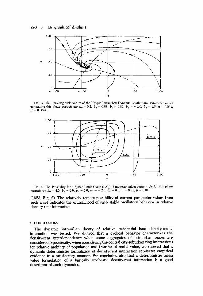
All of the conclusions above critically hinge upon the premise that the parameters shared by all SMSAs (one may say the “environment”) will remain constant over time. This is rather unrealistic for very long term time horizons. However, the model is capable of predicting that the qualitative nature of the dynamic equilibria will always be sink-spiral types, as shown in Figure 3. There is a very small chance that certain key thresholds (extensively discussed in Haag and Dendrinos 1983) may be reached. A phase transition will occur there so that the stable focus will be transformed into a stable limit cycle. A particular set of parameter values capable of resulting in such phase portrait is provided in Figure 4. Figure 5 shows the whole phase portrait. Note that the negativity of b3 makes the actual phase portrait the north-south mirror image of the original scheme found in Haag and Dendrinos

298 / Geographical Analysis

Y

1 .oo

.75

.50

.25

0 - 1.00 - .50 0 .so 1.00

X

FIG. 3. The Spiraling Sink Nature of the Unique Intraurban Dynamic Equilibriuin. Parameter values generating this phase portrait are bo = 0.2, b , = 0.68, b2 = 0.82, b, = - 1.0, 6, = 1.5, a = 0.031, p = 0.0047.

1.00

.75

.25

0 - 1.00 - .so 0 .so 1 .oo

X

FIG. 4. The Possibility for a $able Limit Cycle (L.C.). Parameter values responsible for this phase

(1983, Fig. 2). The relatively remote possibility of current parameter values from such a set indicates the unlikelihood of such stable oscillatory behavior in relative density-rent interaction.

portrait are bo = 4.0, b , = 6.0, b, = 3.0, b, = - 2.0, b4 = 6.0, a = 0.01, p = 0.01.

4. CONCLUSIONS

The dynamic intraurban theory of relative residential land density-rental interaction was tested. We showed that a cyclical behavior characterizes the density-rent interdependence when some aggregates of intraurban zones are considered. Specifically, when considering the central city-suburban ring interactions for relative mobility of population and transfer of rental value, we showed that a dynamic deterministic formulation of density-rent interaction replicates empirical evidence in a satisfactory manner. We concluded also that a deterministic mean value formulation of a basically stochastic density-rent interaction is a good descriptor of such dynamics.

Dimitrios S . Dendrinos and Giinter Haug / 299

FIG. 5. The Isoclines, Selective Trajectories, and the Steady State in’the Whole Phase Portrait ( - 1 d x, y d + 1). Parameter values as in Figure 3.

APPENDIX

Data and Sources Used

Twelve SMSAs are used in this study: Altoona (Pa.), Atlantic City (N.J.), Buffalo (N.Y.), Erie (Pa.), Miami (Fla.), Omaha (Nebr.), Philadelphia (Pa.), Pittsburgh (Pa.), Portland (Oreg.), San Diego (Calif.), Spokane (Wash.), and Trenton (N.J.). They were selected on the basis of the following five criteria: (a) unchanged county composition during the study period (1950-80); (b) one central city; (c) tracted in 1950; (d) SMSAs’ population more than 250,000 in 1960 and 500,000 in 1970; and (e) tract data available in published form by the end of 1982-the time of the study. The number and variety of the SMSAs studied (in terms of age, regional location, and size) does allow for a meaningful analysis and testing of the major hypotheses of the theoretical model.

Three types of time series data are used: central city and suburban population counts; central city to suburb and suburb to central city migration data; and central city and suburban average rental payment per unit area of land. Population series, broken down by central city and suburban ring, are readily available: for the years 1950, 1960, 1970, and 1980 from the decennial Census of Population reports, and for the years 1973, 1975, 1976, 1977, and 1978 from the US. Statistical Abstract, Metropolitan statistics, various years (1974 upward). In case a significant change occurred in the size of certain SMSAs’ central city from 1950 to 1980, only decennial census data are used for these urban areas. Otherwise, data available on an annual basis in the 1970s are also used.

Intraurban migration counts are used for the two time periods: 1955-60 and 1965-70, from the Census of Pqmlation reports. Table 4 “Characteristics of the Population Five Years Old and Over by Mobility Status for SMSAs of 250,000 or More,” or 1960; Table 15 “Mobility Status of the Total and Negro Population of Each SMSA of 500,OOO or More,” for 1970. In the case of the 1955-60 migration counts, yearly average for the fiveyear period is used as the 1959-60 count rather

300 / GeographicalAnalysis

than the actual one in order to be consistent with the 1969-70 count. The 1975-80 counts were not available in printed form at the time of the study.

Rental data per unit area of land are not available from the Bureau of the Census. Instead rental data for dwelling units are used and then appropriately transformed as will be indicated shortly. Data on median rents, and total (renter, owner-occupied, and vacant) dwellings are used by census tract from the four decennial Census of Population reports (1950,1960,1970,1980). A complete list of census tracts used in each SMSA for its central city is available upon request from the authors. The references for these data sets are

1950: U.S. Census of Population, Census Tract Statistics, SMSA. Table 1, Characteristics of the Population, by Census Tracts; Table 3, Characteristics of Dwelling Units, by Census Tracts.

1960: U.S. Census of Population and Housing, Census Tracts, SMSA. Table P-1, General Characteristics of the Population, by Census Tracts, 1960; Table H-1, Occupancy and Structural Characteristics of Housing Units, by Census Tracts, 1960; Table H-2, Year Moved into Unit, Automobile Available, and Values or Rent of Occupied Housing Units, by Census Tracts.

1970: Census of Population and Housing, Census Tracts, SMSA. Table P-1, General Characteristics of the Population, 1970; Table H-1, Occupancy, Utilization, and Financial Characteristics of Housing Units.

1980: Census of Population and Housing, Block Statistics, SMSA. Table 1, Characteristics of Population and Housing Units, for Blocked Portions of the SMSA, 1980; Table 2, Characteristics of Population and Housing Units by Blocks.

Areal data for SMSAs and their central cities were obtained from county level statistics. Where the central city area had to be computed, areal estimates were obtained from census block maps.

Variable y (the r / R count in the model) is computed from rental data, dwelling units count, and area as follows: the ri is obtained by multiplying the total number of dwelling units in inner ring by the median (assumed to equal the average) rent in central city for renter-occupied dwellings, and then the product is divided by the total amount of land in the inner ring. Equivalently, rj for the suburban ring is computed. Variable r is then directly found through equations (2.1) and (2.2). Since the purpose of this aggregate model is to allow for interurban comparisons, spreading the total rental bill over the whole space (in both central city and suburban rings) does not seem to be restrictive.

Because of data limitations, we validated only the qualitative aspects of the phenomenon studied. The precise quantitative measure of intraurban behavior must wait for an extension of the data series over a long time period. This will ultimately determine the validity of the assumption regarding constancy of the model parameters over space and time.

LITERATURE CITED

Dendrinos, D. S., and H. MullaUy (1981). “Evolutionary Patterns of Metropolitan Populations.”

Haag, G., and D. S. Dendrinos (1983). “Toward a Stochastic Dynamical Theory of Location: A

Weidlich, W., and G. Haag (1983). Concepts and Models of a Quantitatioe Sociology. New York:

Geographical Analysis, 13, 328-44.

Nonlinear Migration Process.” Geographical Analysis, 15, 269-86.

Springer-Verlag.