1

A Stochastic Dynamic Controller for Random Early Detection QueuesUsing A Kalman Filter Algorithm

Hamed M. K. Alazemi∗ Mohamed F. Hassan† Mohamed Zribi†∗Computer Engineering Department, Kuwait University

P.O. Box 5969 Safat. Code 13060 Kuwait†Department of Electrical Engineering, Kuwait University

P.O. Box 5969 Safat. Code 13060 Kuwait

Abstract

The stabilizing Random Early Detection (RED) congestion control algorithm in TCP/IP networks is essentially a controltheory problem. Significant attention has been drawn to this problem in the networking and control theory research communities.In this paper, we use a nonlinear dynamic model of the Transmission Control Protocol (TCP) Random Early Detection (RED)congestion control algorithm to analyze and design Active Queue Management (AQM) control systems. A linearized model ofRED behavior around its nominal operating point which implicitly includes the delay in the control signal is derived. It is assumedthat the system model is corrupted at the input and output by zero mean white Gaussian noise signals. An optimal state feedbackstochastic controller is designed for the linearized model of the system in conjunction with a Kalman filter for state estimation.To illustrate the proposed design methodology, simulations results are presented and discussed. The proposed stochastic controlleris applied to the nonlinear model of the system; it is found that the proposed estimator based control scheme works well.

I. Introduction

In recent years, most popular Internet infrastructure routers support some form of congestion control algorithms. One ofthe most popular known algorithms is the Random Early Detection (RED) [?] queue management which is an integral part ofthe transmission control protocol (TCP), the most widely deployed protocol suite in the Internet. Basically, a RED gatewaymaintains an exponentially weighted moving average queue length for detecting persistent congestion, which is characterizedby a switch buffer that is relatively full for a long period of time. The average buffer occupancy is then mapped to a packetdrop probability through a piecewise linear transformation. Specifically, the average queue length is compared to two thresholdvalues, a minimum threshold (minth) and a maximum threshold (maxth). When the average queue length is smaller thanminth, no arriving packets aremarked/dropped. When the average queue length is betweenminth and maxth, packets aremarked/dropped with a probability that increases linearly as a function of the average buffer occupancy, reaching a maximumdrop probability (maxp) at the maximum threshold. A detailed stochastic model of RED can be found in [?] and the referencestherein.

Random early detection algorithms allow buffering of transient bursts (by temporarily increasing the queue), as long as theyare noticeably shorter than the queue averaging interval. The basic idea behind RED queue management algorithm is to detectincipient congestion early and to send congestion notification to the TCP sources in the network, allowing them to reduce theirtransmission rates before the queues in the network overflow. Accordingly, the objectives of this idea are to minimize packetloss and queuing delay, to avoid global synchronization of sources, and to maintain high link utilization. However, RED isknown to have sensitivity to its parameter settings and to the changes in the link’s traffic load [?]. Within this realm, researchershave shown that getting appropriate values of RED parameters that show good performance under different congestion scenariosremains an inexact science [?]. Therefore, many different variants of RED have been proposed, such as BLUE [?], SRED [?],and Exponential-RED [?].

On the analytical front, there have been numerous studies on Active Queue Management (AQM) in recent years. Of particularinterest to us is the work related to controllability and stability of TCP/IP congestion control algorithms [?], [?], [?], [?], [?],[?], [?], [?]. In particular, studies that model TCP congestion control mechanism as a feedback dynamic system through controltheory analysis have shown tremendous insight into the design and modeling of efficient TCP/IP gateways. In [?], for example,the authors developed a fluid based modeling approach for TCP connections in a network that features AQM routers. Thisapproach, which uses jump process driven stochastic differential equations to characterize the interactions of a set of TCP flowsand AQM routers in a network setting, models TCP behavior that includes the transient effects introduced by AQM routerssuch as RED gateways. In [?], the authors used linearization to analyze a previously developed nonlinear model of TCP whichwas presented in [?]. They performed the analysis on an AQM system implementing RED; they presented design guidelines forchoosing parameters which lead to local stability. Their analysis uncovered the limitations of the averaging algorithm in RED.In addition, proportional and proportional-integral controllers have been proposed as AQM strategies with faster responses thanthe RED controller. In [?], [?] the AQM congestion control was viewed as a convex optimization problem for the dynamicsystem.

Several researchers have proposed controllers for the system under consideration using different models of the system, forexample see [?], [?], [?], [?], [?], [?]. Amongst the aforementioned studies, the work in [?] carries the most relevance to thework presented in this paper. The authors in [?] consider the design of explicit rate-based congestion control for high-speedcommunication networks and show that this can be formulated as a stochastic control problem where the controls of different

users enter the system dynamics with different delays. They formulate the congestion control problem as an LQG stochasticcontrol problem, and present two algorithms for rate control that are derived using tools from stochastic control theory. Otherclassical studies in this subject that is of important relevance to the work presented here can be found in [?], [?], [?]. To thebest of our knowledge, this is the first work which uses a stochastic model to represent the behavior of the system. Hence,the contribution of the paper is on using a stochastic model to represent the system and then using a Kalman filter basedsub-optimal control scheme to control the original nonlinear system.

This paper is organized as follows. Section 2 presents the nonlinear model which describes the behavior of the TCP; alinearized model for TCP behavior around its nominal operating point which implicitly includes the delay in the control signalis derived. Section 3 proposes an optimal stochastic controller for the linearized TCP model. Simulation results are presentedand discussed in Section 4. Finally, some concluding comments are given in Section 5.

II. Model of the TCP Behavior

The dynamic behavior of TCP was developed in [?], [?], [?] using fluid flow and stochastic differential equation analysis.In [?] a simplified version of that model which ignores the TCP timeout and the slow start phase was used. This model, whichrelates the average value of the key network variables, is used in the analysis and development of this paper. Accordingly, thedynamic behavior of TCP is characterized by the following coupled, highly nonlinear differential equations:

W (t) =1

R(t)− W (t)W (t−R(t))

2R(t−R(t))p(t−R(t))

q(t) =W (t)R(t)

N(t)− C (1)

where,

• W ∈ [0, W ] is the expected TCP window size (packets),• W is the maximum window size,• q ∈ [0, q] is the expected queue length (packets),• q is the buffer capacity,• R is the round trip time (RTT),• C is the link capacity (packets/sec),• Tp is the propagation delay (seconds),• N is the load factor (number of TCP sessions), and• p ∈ [0, 1] is the probability of packet mark/drop.

Note that the round trip time is defined as:

R(t) =q(t)C

+ Tp (2)

Our development is based on small signal linearization around the operating point [?]. Let (Wo, qo, po) be the operatingpoint defined by settingW = 0 and q = 0. Then,

W = 0 =⇒ W 2o po = 2

q = 0 =⇒ Wo =RoC

N(3)

where

Ro =qo

C+ Tp (4)

Assuming thatN(t) = N andR(t) = Ro are constants, we linearize model (1) around the operating point(Wo, qo, po). Let,

δW (t) = W (t)−Wo

δp(t) = p(t)− po

δq(t) = q(t)− qo (5)

The linearized model can be written as:

δW (t) = − N

R2oC

[δW (t) + δW (t−Ro)]− RoC2

2N2δp(t−Ro)

δq(t) =N

RoδW (t)− 1

Roδq(t) (6)

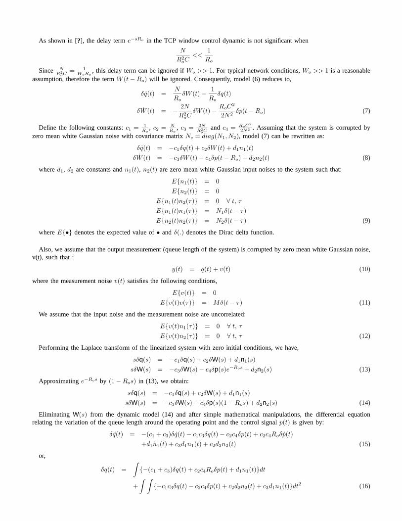
As shown in [?], the delay terme−sRo in the TCP window control dynamic is not significant when

N

R2oC

<<1

Ro

Since NR2

oC = 1WoRo

, this delay term can be ignored ifWo >> 1. For typical network conditions,Wo >> 1 is a reasonableassumption, therefore the termW (t−Ro) will be ignored. Consequently, model (6) reduces to,

δq(t) =N

RoδW (t)− 1

Roδq(t)

δW (t) = − 2N

R2oC

δW (t)− RoC2

2N2δp(t−Ro) (7)

Define the following constants:c1 = 1Ro

, c2 = NRo

, c3 = 2NR2

oC and c4 = RoC2

2N2 . Assuming that the system is corrupted byzero mean white Gaussian noise with covariance matrixNc = diag(N1, N2), model (7) can be rewritten as:

δq(t) = −c1δq(t) + c2δW (t) + d1n1(t)δW (t) = −c3δW (t)− c4δp(t−Ro) + d2n2(t) (8)

whered1, d2 are constants andn1(t), n2(t) are zero mean white Gaussian input noises to the system such that:

E{n1(t)} = 0E{n2(t)} = 0

E{n1(t)n2(τ)} = 0 ∀ t, τ

E{n1(t)n1(τ)} = N1δ(t− τ)E{n2(t)n2(τ)} = N2δ(t− τ) (9)

whereE{•} denotes the expected value of• andδ(.) denotes the Dirac delta function.

Also, we assume that the output measurement (queue length of the system) is corrupted by zero mean white Gaussian noise,v(t), such that :

y(t) = q(t) + v(t) (10)

where the measurement noisev(t) satisfies the following conditions,

E{v(t)} = 0E{v(t)v(τ)} = Mδ(t− τ) (11)

We assume that the input noise and the measurement noise are uncorrelated:

E{v(t)n1(τ)} = 0 ∀ t, τ

E{v(t)n2(τ)} = 0 ∀ t, τ (12)

Performing the Laplace transform of the linearized system with zero initial conditions, we have,

sδq(s) = −c1δq(s) + c2δW(s) + d1n1(s)sδW(s) = −c3δW(s)− c4δp(s)e−Ros + d2n2(s) (13)

Approximatinge−Ros by (1−Ros) in (13), we obtain:

sδq(s) = −c1δq(s) + c2δW(s) + d1n1(s)sδW(s) = −c3δW(s)− c4δp(s)(1−Ros) + d2n2(s) (14)

Eliminating W(s) from the dynamic model (14) and after simple mathematical manipulations, the differential equationrelating the variation of the queue length around the operating point and the control signalp(t) is given by:

δq(t) = −(c1 + c3)δq(t)− c1c3δq(t)− c2c4δp(t) + c2c4Roδp(t)+d1n1(t) + c3d1n1(t) + c2d2n2(t) (15)

or,

δq(t) =∫{−(c1 + c3)δq(t) + c2c4Roδp(t) + d1n1(t)}dt

+∫ ∫

{−c1c3δq(t)− c2c4δp(t) + c2d2n2(t) + c3d1n1(t)}dt2 (16)

c2c4 d1c3 c2d2

c1c3 c1+c3

c1c4Ro d1

y(t)

v(t)

+ + x1=δq x2 + +

+

-

+ +

-

-

δp(t) n1(t) n2(t)

Fig. 1. Simulation diagram

With the output measurement as given above, the simulation diagram representing (10) and (16) is shown in Fig. 1.Now, choose the state variablesx1 andx2 as defined in Fig. 1. Then the state equations describing the linearized behavior

of the TCP model is given by:

x(t) = Axx(t) + Bxu(t) + Dxn(t)y(t) = Hx(t) + v(t) (17)

where

x(t) =[

x1(t)x2(t)

], n(t) =

[n1(t)n2(t)

], u(t) = δp(t)

and,

Ax =[ −(c1 + c3) 1

−c1c3 0

], Bx =

[c2c4Ro

−c2c4

], Dx =

[d1 0

c3d1 c2d2

], H =

[1 0

]

The transformation between the state variable vectorx(t) defined in (17) and the original state variables of the system

z(t) = [δq(t) δW (t)]T is given by:

x(t) = T1z(t) + T2u(t) (18)

where,

T1 =[

1 0c3 c2

]and T2 =

[0

−c2c4Ro

](19)

We now have a linearized model for TCP behavior around its nominal operating point which implicitly includes the delayin the control signal. Our main interest in this paper is to derive a closed loop optimal stochastic dynamic controller whichguarantees the optimal system performance as well as asymptotic stability of the system. This will be developed in the nextsection.

III. Stochastic Dynamic Controller for the System

A. Discretized Model and Properties

Discretization of the system model (17) using a discrete time interval∆T , leads to the following:

x(k + 1) = Φ(k + 1, k)x(k) + Ψ(k + 1, k)u(k) + Γ(k + 1, k)n(k)y(k + 1) = H(k + 1)x(k + 1) + v(k + 1), k ∈ [ko, ..., kf − 1] (20)

whereΦ(k + 1, k) ∈ IR2×2 is the state transition matrix,Ψ(k + 1, k) ∈ IR2×1 is the control transition matrix,Γ(k + 1, k) ∈IR2×2 is the disturbance transition matrix, andH ∈ IR1×2 is the measurement matrix.

The above model is a first orderMarkov process which has the following properties.

• P1 x(k) is a Gaussian random process (or approximated by a Gaussian process for which the mean and covariance arethe first two moments of the Poisson process) with the following properties:

E{x(k)} = 0E{x(ko)} = xo

E{x(ko)xT (ko)} = P (ko) (21)

• P2 The input noise vectorn(k) is zero mean white Gaussian with covariance matrixNc,

E{n(k)} = 0E{n(k)nT (l)} = Ncδ(k − l) (22)

whereδ(k − l) is the dirac-delta function defined such thatδ(k − l) = 1 for k = l andδ(k − l) = 0 for k 6= l.• P3 The measurement noisev(k) is zero mean white Gaussian with covarianceM ,

E{v(k)} = 0E{v(k)vT (l)} = Mδ(k − l) (23)

• P4 The state vectorx(k) and the input noise vectorn(l) are uncorrelated forl ≥ k,

E{x(k)nT (l)} = 0 for l ≥ k (24)

• P5 The state vectorx(k) and the measurement noisev(l) are uncorrelated,

E{x(k)vT (l)} = 0 ∀ l, k (25)

• P6 The input noise vectorn(k) and the measurement noisev(l) are uncorrelated,

E{n(k)vT (l)} = 0 ∀ l, k (26)

• P7 The initial state vectorx(ko) and the input noise vectorn(k) are uncorrelated,

E{x(ko)nT (k)} = 0 ∀ k (27)

• P8 The initial state vectorx(ko) and the measurement noisev(k) are uncorrelated,

E{x(ko)vT (k)} = 0 ∀ k (28)

• P9 The output vectory(k) and the measurement noisev(l) are uncorrelated forl > k

E{y(k)vT (l)} = 0 for l > k (29)

It should be noted that not all the states are available for feedback (i.e., the stateδW is not measurable for the model ofthe TCP behavior). Hence, the design of the state feedback controller will be accomplished in 2 steps. The first one dealswith the design of an optimal control scheme for the system; the second one deals with the design of an estimator (Kalmanfilter) to estimate the states of the system. Then the estimated states are used to control the process. Because of the separationprinciple [?], these two steps are independent of each other (i.e., the design of the controller is separate from the the designof the estimator).

B. Design of the Optimal Controller

The objective of the paper is to design an optimal control scheme for the system. Consider the discrete time control system

x(k + 1) = Φ(k + 1, k)x(k) + Ψ(k + 1, k)u(k) + Γ(k + 1, k)n(k)y(k + 1) = H(k + 1)x(k + 1) + v(k + 1), k ∈ [ko, ..., kf − 1] (30)

with initial condition x(ko). We choose the performance performance indexJ such that:

J = E

12

kf−1∑

k=ko

(xT (k + 1)Qx(k + 1) + uT (k)Ru(k)

)

= E

12

kf−1∑

k=ko

(||x(k + 1)||2Q + ||u(k)||2R) (31)

whereQ is a symmetric positive semi-definite matrix andR is a symmetric positive definite matrix. We seek to design anoptimal controller such that the performance indexJ in (31) is minimized subject to the model (30).

It is well known that

min J = min E

12

kf−1∑

k=ko

(||x(k + 1)||2Q + ||u(k)||2R)

= min Ey

Ex/y

1

2

kf−1∑

k=ko

(||x(k + 1)||2Q + ||u(k)||2R) | y(ko + 1), ..., y(k)

(32)

whereEy is the expected value ofy andEx/y is the expected value ofx given y.Sincey(ko + 1), . . . , y(k) are given, equation (32) reduces to [?]:

min J = min Ex/y

12

kf−1∑

k=ko

(||x(k + 1)||2Q + ||u(k)||2R) | Y (k)

(33)

whereY (k) = [y(ko + 1), y(ko + 2), ..., y(k)]T .The following fact gives the optimal controller for the system.FACT 1:Given the model (30), the control signal which minimizes (31) and hence (33) is given by:

u(k) = G(k)x(k/k) (34)

whereG(k) is the closed loop gain matrix of the corresponding state feedback optimal linear quadratic problem which is givenby:

G(k) = −R−1ΨT (k + 1, k)Φ−T (k + 1, k) [K(k)−Q] (35)

= −R−1ΨT (k + 1, k)K(k + 1)[I + Ψ(k + 1, k)R−1ΨT (k + 1, k)K(k + 1)

]−1Φ(k + 1, k)

andK(k) is the solution of the matrix difference Riccati equation (DRE):

K(k) = Q + ΦT (k + 1, k)K(k + 1)[I + Ψ(k + 1, k)R−1ΨT (k + 1, k)K(k + 1)

]−1Φ(k + 1, k)

with K(kf ) = [0] (36)

and x(k/k) is the estimate of x(k) given the measurementsY (k).Proof: see reference [?].

Since not all states are available for feedback, we next discuss an estimator for the state vector.

C. Design of the Kalman Filter

It is desired to design an optimal estimator for the states of the system when additive input and output noise noise arepresent in the process.

Let x(k/k) and y(k/k) denote the estimates ofx(k) and y(k) respectively knowing the measurement vectorY (k). Letx(k/k − 1) denotes the estimate ofx(k) which obtained using the measurements available up to the time instantk − 1, theestimation errorsx(k/k − 1) and y(k/k − 1) are defined as follows:

x(k/k − 1) = x(k)− x(k/k − 1) (37)

y(k/k − 1) = y(k)− y(k/k − 1) (38)

In addition, define the following covariance matrices:

P (k/k − 1) = Pxx(k/k − 1)= E{x(k/k − 1)xT (k/k − 1)}= Φ(k, k − 1)P (k − 1/k − 1)ΦT (k, k − 1) + Γ(k, k − 1)NcΓT (k, k − 1)

with P (ko/ko) = P (ko) (39)

Pxy(k/k − 1) = E{x(k)yT (k/k − 1)} = E{x(k/k − 1)yT (k/k − 1)}= P (k/k − 1)HT (40)

Pyy(k/k − 1) = E{y(k/k − 1)yT (k/k − 1)}= HP (k/k − 1)HT + M (41)

The task is to design an estimator which minimizes the cost function:

J = E{(x(k)− x(k/k))T (x(k)− x(k/k))}= Ex/Y {(x(k)− x(k/k))T (x(k)− x(k/k))/Y (k)} (42)

FACT 2:The optimal Kalman filter state estimator given by:

x(k/k) = x(k/k − 1) + L(k) [y(k)− y(k/k − 1)] (43)

where,

L(k) = Pxy(k/k − 1)P−1yy (k/k − 1) = P (k/k − 1)HT [HP (k/k − 1)HT + M ]−1 (44)

P (k/k) = [I − L(k)H]P (k/k − 1) (45)

x(k/k − 1) = Φ(k, k − 1)x(k − 1/k − 1) + Ψ(k, k − 1)u(k) with x(ko/ko) = xo (46)

y(k/k − 1) = Hx(k/k − 1) (47)

which minimizes the cost function (42) and guarantees the asymptotic stability of the estimator error.Proof: see reference [?].

Remark 1: The estimator (Kalman-filter) based control scheme which minimizes (31) subject to the model (30) is givenby:

u(k) = G(k)x(k/k) (48)

Remark 2: It is important to note that the optimal closed loop gain matrixG(k) can be calculated off-line and stored in thecomputer. Hence, the optimal control signalu(k) is calculated based on the Kalman filter estimator of the state vectorx(k/k).

Remark 3: It is important to note that the controller (34) is optimal when it is applied to the linear model (30). However,the controller is sub-optimal if it is applied to the nonlinear model of the system (1).

IV. SIMULATION RESULTS

In order to show the effectiveness of the proposed design, the developed closed loop dynamic stochastic controller is used tocontrol the queue length of a TCP system. Although our analysis and design are based on a linearized model, our simulationsare carried out on the nonlinear system.

Fig. 2 shows a block diagram representation of the system to be simulated.

The data used in the simulations are taken from the literature [?]. The following numerical values are considered:C = 3750packets,Ro ≤ 0.25 is taken to be 0.2;N > 1

5π N− = 15π 60 = 3.82, henceN is taken to be 4. The discretization time,

∆T = 0.01sec. The matrixQ is taken to be the identity matrix, I; R = 105; P (0) = 25I; Nc = diag(N1, N2), whenN1 andN2 will be specified later on,M = 1, d1 = 1 andd2 = 10e− 8.

)/( kkx∧

Original nonlinear TCP system model

Delay

Kalman filter for the linearized System model

G(k)

y(k)

u(k)=δp(k)

Fig. 2. Block diagram of the simulated system

It should be noted that, to avoid very large numbers in the matrices of the system, more specificallyΨ(k+1, k), the followingvariables of the model are normalized to the line capacityC such that:

x′1(k) =

1C

x1(k)

x′2(k) =

1C

x2(k)

n′1(k) =

1C

n1(k)

n′2(k) =

1C

n2(k)

v′(k) =

1C

v(k)

Ψ′(k + 1, k) =

1C

Ψ(k + 1, k)

Therefore, the normalized linear model used in our simulation is given by:

x′(k + 1) = Φ(k + 1, k)x

′(k) + Ψ

′(k + 1, k)u(k) + Γ(k + 1, k)n

′(k)

y′(k + 1) = H(k + 1)x

′(k + 1) + v

′(k + 1) (49)

k ∈ [ko, ..., kf − 1]

whereH is our case is constant and independent of time.Also it is important to note the following:1- Although the output of both the linearized model given by (17) and the original nonlinear model (1) are the same, namely

the queue length, the second state variable in the linearized one is not the window size. In order to show the effectiveness of theestimator resulting from the Kalman filter which is actually used in calculating the optimal control signal, the transformationmatrices given in (19) are used to calculate the window size obtained from the estimator and then used in our plots with thatresulted from our simulated nonlinear model.

2- In all our plots, the state vectors are de-normalized and the steady state values are added to the de-normalized estimatedstate variables.

Three simulation are done for three case studies. The first case corresponds to no input noise (i.e.,N1 = 0, N2 = 0). Thesecond case corresponds to small input noise (i.e.,N1 = 10, N2 = 1); the third case corresponds to large input noise (i.e.,N1 = 100, N2 = 100).

The Kalman filter based controller is applied to the nonlinear model (1). The simulation results are shown in Fig. 3 - Fig.11. Fig. 3 shows the actual and estimated queue lengths for the no input noise case; it is clear that the size of the queue startsfrom 100 and converges to zero in about 3 seconds. Fig. 3 also shows that the error between the actual and the estimatedvalues of the queues in initially large and converges to a small value ast gets larger. Fig. 4 shows the actual and estimatedwindow sizes for the no input noise case. It is clear that the window size start around 220 and converges to about 187; theerror between the actual and the estimated window size converges to zero as t gets larger. Fig. 5 shows the control action forthe no input noise case. Fig. 6 shows the actual and estimated queue lengths for the small input noise case. Fig. 7 shows theactual and estimated window sizes for the small input noise case. Fig. 8 shows the control action for the small input noisecase. Fig. 9 shows the actual and estimated queue lengths for the large input noise case. Fig. 10 shows the actual and estimatedwindow sizes for the large input noise case. Fig. 11 shows the control action for the large input noise case. It is clear fromFig. 6, Fig. 7, Fig. 9 and Fig. 10 that the noise affects the performance of the system; however, even with the existence of

large noise the controlled system behaved rather well. Therefore, it can be concluded that results of the simulations indicatethat the proposed estimator based controller works well.

Remark 4: The nonlinear model (1) can be made to be more realistic if clipping is added since the queue length and thewindow size should be greater or equal to zero. Simulations results indicate that the proposed estimator based controller workswell even if clipping is added to the model. However, more analysis is required for this case in order to study the impact ofclipping on the nature of the process.

V. CONCLUSION

The paper deals with the stochastic stabalization of a AQM/TCP model. The nonlinear model of the system which containsinput delay is linearized and a model which implicitly includes the delay in the control signal is derived. Zero mean whiteGaussian noise signals are added to the process input and output measurements. An optimal controller is proposed for thelinearized system and a Kalman filter is used to estimate the states. The proposed controller is sub-optimal when applied to theoriginal nonlinear model of the system. The proposed design procedure is illustrated through simulation results. The stochasticcontroller is applied to the nonlinear model of the system. Simulation results indicate that the proposed controller keeps thequeue length within bounds in an appropriate stochastic sense.

Future work will address the control of a multi-node TCP model needs to be investigated.

0 0.5 1 1.5 2 2.5 3−20

0

20

40

60

80

100

120actual qestimated q

Fig. 3. Actual and estimated queue lengths versus time (no input noise)

0 0.5 1 1.5 2 2.5 3180

190

200

210

220

230

240

250

260actual Westimated W

Fig. 4. Actual and estimated window size versus time (no input noise)

0 0.5 1 1.5 2 2.5 3−0.5

0

0.5

1

1.5

2

2.5

3

3.5x 10

−3

Fig. 5. Control signal versus time (no input noise)

0 2 4 6 8 10−20

0

20

40

60

80

100

120actual qestimated q

Fig. 6. Actual and estimated queue lengths versus time (small input noise)

0 2 4 6 8 10180

190

200

210

220

230

240

250

260actual Westimated W

Fig. 7. Actual and estimated window size versus time (small input noise)

0 2 4 6 8 10−0.5

0

0.5

1

1.5

2

2.5

3x 10

−3

Fig. 8. Control signal versus time (small input noise)

0 2 4 6 8 10−60

−40

−20

0

20

40

60

80

100

120actual qestimated q

Fig. 9. Actual and estimated queue lengths versus time (large input noise)

0 2 4 6 8 10160

170

180

190

200

210

220

230

240

250

260actual Westimated W

Fig. 10. Actual and estimated window size versus time (large input noise)

0 2 4 6 8 10−1.5

−1

−0.5

0

0.5

1

1.5

2

2.5

3

3.5x 10

−3

Fig. 11. Control signal versus time (large input noise)