Comput Geosci (2012) 16:455–466DOI 10.1007/s10596-011-9238-2

ORIGINAL PAPER

Sampling error distribution for the ensemble Kalman filterupdate step

Andrey Kovalenko · Trond Mannseth · Geir Nævdal

Received: 31 January 2011 / Accepted: 30 May 2011 / Published online: 6 July 2011© The Author(s) 2011. This article is published with open access at Springerlink.com

Abstract In recent years, data assimilation techniqueshave been applied to an increasingly wider specterof problems. Monte Carlo variants of the Kalmanfilter, in particular, the ensemble Kalman filter (EnKF),have gained significant popularity. EnKF is used fora wide variety of applications, among them for up-dating reservoir simulation models. EnKF is a MonteCarlo method, and its reliability depends on the actualsize of the sample. In applications, a moderately sizedsample (40–100 members) is used for computationalconvenience. Problems due to the resulting MonteCarlo effects require a more thorough analysis of theEnKF. Earlier we presented a method for the assess-ment of the error emerging at the EnKF update step(Kovalenko et al., SIAM J Matrix Anal Appl, in press).A particular energy norm of the EnKF error aftera single update step was studied. The energy normused to assess the error is hard to interpret. In thispaper, we derive the distribution of the Euclidean normof the sampling error under the same assumptions asbefore, namely normality of the forecast distribution

A. Kovalenko (B) · T. MannsethUni CIPR, P.O. Box 7810, 2050 Bergen, Norwaye-mail: andrey.kovalenko@uni.no

T. Mannsethe-mail: trond.mannseth@uni.no

A. Kovalenko · T. Mannseth · G. NævdalDepartment of Mathematics, University of Bergen,Bergen, Norway

G. NævdalInternational Research Institute of Stavanger,Bergen, Norwaye-mail: Geir.Naevdal@iris.no

and negligibility of the observation error. The distrib-ution depends on the ensemble size, the number andspatial arrangement of the observations, and the priorcovariance. The distribution is used to study the errorpropagation in a single update step on several syntheticexamples. The examples illustrate the changes in relia-bility of the EnKF, when the parameters governing theerror distribution vary.

1 Introduction

Maximizing the hydrocarbon production requires sub-stantial knowledge of the reservoir. Properties of reser-voir rocks and fluids are used in mathematical models,which are in turn used to predict the reservoir’s futurebehavior. Accurate predictions are essential for suc-cessful hydrocarbon recovery. Since direct observationof each and every point in the reservoir is technicallyimpossible, one cannot populate a reservoir model withexactly known values. The observation techniques usedto acquire the reservoir properties before productionstarts are either local (wireline logs and formation tests)or to a large degree imprecise (seismic surveys). Due tothese reasons, reservoir models operate with uncertainparameters and forecasts of the reservoir behavior are,in turn, also uncertain. Reducing the uncertainty ofthe forecasts plays a crucial role in the hydrocarbonrecovery process.

In order to improve the forecasts, the reservoirmodel needs to be adjusted with the information fromproduction data. Time-lapse seismic data can also beused in updating reservoir models, see, e.g., [1, 6, 13].Adjusting the model parameters based on the observed

456 Comput Geosci (2012) 16:455–466

data is known as history matching. Improving the un-certain reservoir model is done by assuming the reser-voir fluid and rock properties to be random values. Thereservoir states, i.e., pressures and saturations, are inthis case also random. A widely used methodology tocondition the states and parameters on observationsis the Bayesian framework. The poorly known reser-voir states and parameters are associated with theirrespective probability density functions. Combining thesystem state, u(x, t), and the system parameters, μ(x),into a single vector θ(x, t) = (u(x, t), μ(x))T , one candefine a joint density function, f (θ). Further, for theobservations, denoted as d(x, t), one defines a likeli-hood distribution f (d|θ). Using Bayes’ rule, one maydirectly write

f (θ |d) ∝ f (θ) f (d|θ). (1)

Since history matching is based on sequential datasets (production records, time-lapse seismic surveys,etc.), it is natural to adjust the reservoir model as thedata are available. The sequential process of updatingthe system state and parameters by incorporating a se-ries of measured data into the numerical model is calleddata assimilation. The purpose of data assimilation inthe Bayesian setting is to find the posterior joint proba-bility distribution of the reservoir states and parametersconditioned on the series of observed dynamic data.

Generally, the extended model state, θ(x, t), is acontinuous function of time. It is convenient to workwith a model state discretized in time, i.e., θ(x, t) isrepresented at certain time intervals as θk(x) = θ(x, tk),where k = 0, . . . , Nt, and Nt is the total number oftime instances. The extended model state is also dis-cretized in space such that θk = (θk(x1), . . . , θk(xM))T ,where M is the spatial model dimension. The data arerepresented such that dk = dk(x1), . . . , dk(xNd), whereNd is the dimension of the resulting data vector. For thesake of simplicity, we will further assume the extendedmodel state to be discretized in time such that thedata arrive at the same instances, tk. Following Evensenand van Leeuwen [11], we write the expression for theconditional probability function for the discrete timecase:

f (θk|dk, . . . , d1) ∝ f (θk|dk−1, . . . , d1) f (dk|θk). (2)

Reducing Eq. 1 to the discrete form (Eq. 2) is doneunder the assumption of the model evolution to be afirst order Markov process, i.e., θk depends only on θk−1,but not on any of the preceding states, θk−2, . . . , θ0.

In general, finding the posterior density in Eq. 2 isdifficult. In order to make it computationally feasible,

it is assumed that the prior distribution of the extendedstate vector is Gaussian. The density f (θk|dk−1, . . . , d1)

is therefore assumed to be Gaussian with mean θf

k

and covariance C fk , denoted as N (θ

fk , C f

k ). Assuminga linear relationship between model parameters andobservations through the measurement matrix, H, andadding independent Gaussian noise, i.e.,

dk = Hθk + εdk, εd

k ∼ N(0, Cd

k

),

is sufficient for the posterior distribution to beGaussian. The posterior mean and covariance maxi-mize the likelihood function given in Eq. 2. Omittingthe details which can be found, for example, in [10], wemay write the equations for the posterior mean, θa

k , andposterior covariance, Ca

k:

θak = θ

fk + Kk

(dk − Hθ

fk

), (3)

Cak = (I − Kk H)C f

k . (4)

Kk = C fk HT

(HC f

k HT + Cdk

)−1, (5)

Here, K is the Kalman gain matrix. Equations 3–5 areknown as the Kalman filter analysis equations [19].These equations are used to obtain the posterior distri-bution of the extended state vector taking into accountthe observations at the kth time increment. In orderto propagate the system forward in time, the forecastequations are applied:

θf

k = Akθak−1 + εm

k , εmk ∼ N (0, Cm

k ), (6)

C fk = AkCa

k−1 ATk + Cm

k , (7)

where A is a linear operator of system evolution and εm

is a normally distributed model error.For a Gaussian extended state vector and a linear

operator of system evolution, the Kalman filter deliversthe best estimate. In a great number of real problems,application of the Kalman filter is computationallyunfeasible due to the size of the system, even if theforward model is linear. The covariances are too large,and the corresponding matrix equations are difficult tosolve correctly. In case of a non-linear forward model,the assumption of Gaussianity that the Kalman filterrelies on is not satisfied. Applying such an operatorto the Gaussian system state results in a non-Gaussianoutput, thus making direct assessment of the resultingdistribution impossible.

Comput Geosci (2012) 16:455–466 457

In order to deal with these two issues, a MonteCarlo technique is applied. Instead of adjusting thedistribution by running the Kalman filter update andforecast Eqs. 3–7, one estimates the mean and covari-ance from a moderately sized ensemble. Even thoughlittle is known about the ability of such a techniqueto fully describe non-Gaussian distributions, ensemble-based methods are applied to problems with non-linearforward operator.

The most commonly applied data assimilationmethod is the ensemble Kalman filter (EnKF), firstintroduced by Evensen [7]. The method is easy to applyto different state and parameter estimation problems.An extensive description can be found in [10]. It hasbeen applied, for example, to problems in climatology,oceanography, and meteorology, see, e.g., [3, 8, 18].

In oil recovery, the EnKF has been applied forreservoir characterization and history matching, see,e.g., [22, 23, 26]. For an extensive literature review anddiscussion of the methodology, see [2]. For a reviewof recent applications, see [25]. It has also been usedwithin closed-loop reservoir management and produc-tion optimization, see, e.g., [4] and [24].

The EnKF starts out with an ensemble {θai,0}Ne

i=1 fromthe initial distribution. For a (generally nonlinear)model operator, Fk, each ensemble member is updatedas follows:

θf

i,k = Fk(θai,k−1) + εm

i,k, (8)

where εmi,k are the modeling errors, generated indepen-

dently for each sample. The covariance is estimatedfrom the resulting ensemble:

C̃ fk = 1

Ne − 1

Ne∑

i=1

(θ

fi,k − θ̄

fk

) (θ

fi,k − θ̄

fk

)T, (9)

where θ̄ denotes the ensemble mean. Replacing thetrue covariance with its estimate and adding indepen-dent errors to the observed data (the resulting vectorsare denoted as di,k), one performs the analysis stage asin Eqs. 3 and 5:

θai,k = θ

fi,k + K̃k

(di,k − Hθ

fi,k

), (10)

K̃k = C̃ fk HT

(HC̃ f

k HT + Cdk

)−1. (11)

The analyzed sample mean, θ̄ak , and the correspond-

ing sample covariance, C̃ak, computed from the analyzed

ensemble as in Eq. 9 approximate the posterior meanand covariance. It is worth pointing out that in generaleven the exact mean and covariance do not fully char-acterize non-Gaussian distributions, but this issue is not

considered in the current article. Instead, we focus onthe Monte Carlo approximation of the analysis distrib-ution. Further in the article, we will limit ourselves tothe case of linear forward and measurement operators.

Ensemble-based estimation leads to several issues.Sampling error affects both mean and covariance es-timates but vanishes as the ensemble size tends toinfinity. With EnKF, the sampling error depends notonly on the ensemble size but also on the number andmutual locations of measurements, see, for example,[12].

Sampling errors in the covariance matrix estimatelead to spurious correlations, i.e., erratic changes of thestate vector components in regions of no real influence.The most common approach to avoid spurious correla-tions is to perform the update locally, i.e., the extendedstate vector components are updated only if they areclose to the observations [14, 18]. In practice, closenessis often defined somewhat “ad hoc”. If the numberof observations exceeds the ensemble size, the entireensemble can collapse, i.e., the spread of the ensembledecreases gradually with every time step. Ensemblecollapse and localization techniques, however, are notaddressed in the current paper.

With the finite ensemble size, EnKF may experiencerank deficiency. The issue arises due to the lack of thedegrees of freedom (number of ensemble members) toproperly assimilate the measurements, if the ensemblesize is smaller than the number of measurements. Athorough discussion on how to apply the EnKF or itsvariants in this situation can be found in [9, 10]. We willconsider the case when the ensemble size is greater thanthe number of measurements further in the article.

The EnKF is also affected by the relation betweenthe size of the ensemble and the number of assimilateddata points. In [20], e.g., it has been shown that increas-ing the number of measurements leads to degeneracyof the ensemble. In the numerical studies performedin [12], it has been shown that increasing number ofmeasurements leads to loss of quality of the EnKFupdate.

The ensemble of states and parameters updated withthe EnKF provides an estimate of the uncertainty asso-ciated with the reservoir. However, very little is knownabout the accuracy of the method itself. It is possible tobuild an empirical distribution function for the EnKFsampling error, but this approach would require a hugecomputational effort. Thus, in order to approximate thecumulative distribution function with Ns points, oneneeds to run Ne × Ns EnKF updates. In addition, suchan approximation would also be extremely problemdependent.

458 Comput Geosci (2012) 16:455–466

Better understanding of the quality of the EnKFis the purpose of the present paper. We focus on anessential part of the EnKF algorithm, namely the analy-sis step. We study the norm of the sampling error,defined as the difference between the outcomes fromthe Kalman filter analysis equations and their EnKFcounterparts.

In Kovalenko et al., submitted, we obtained a dis-tribution for a particular energy norm of the samplingerror arising at a single EnKF analysis step. We usedseveral results from random matrix theory in order toderive the distribution. The norm of the sampling errorwe used in Kovalenko et al., submitted, however, isnot easy to interpret. In [21], we gave a sketch of thederivation of the distribution for the Euclidean norm.

In the current paper, we derive the distribution ofthe Euclidean norm in full details. The distributiondepends on the system size, number of ensemble mem-bers, prior covariance properties, and mutual locationsof the measurements. In order to obtain the distribu-tion, we make the same assumptions as in Kovalenkoet al., submitted. Namely, we assume the measurementerrors to be negligible, the forecast distribution to beGaussian, and the model and measurement operatorsto be linear. Although one cannot expect to know theexact forecast distribution in a real reservoir character-ization problem, this simplistic setting is still of interestas it can be considered as a “best-case scenario” for theEnKF. It is, however, of great significance to extend theobtained distribution to a real reservoir case.

We also perform a set of numerical experimentsillustrating the behavior of the obtained distribution.For a given reference field and a given prior distribu-tion, we build the distribution of the sampling error invarious situations, as if we were to perform the EnKFupdates of the state vector. We vary the parametersthe distribution depends on in order to investigate theirinfluence on the quality of the EnKF update. The ana-lytical distribution is then compared with the empiricaldistribution of the sampling error norm.

The paper is organized as follows: Section 2 givesan overview of certain results from random matrixtheory used to derive the main result. Section 3 con-tains the derivation of the main result. The section issplit into two parts. In the first subsection, we give ashortened derivation of the result from Kovalenko etal., submitted, given here for the sake of completeness.The second subsection contains the extension of thederivation to the case of the Euclidean norm, givenin full details. Section 4 is dedicated to the numericalexperiments. Finally, we give an outlook and review thepossibilities for future extensions.

2 Some properties of random matrices

The EnKF analysis step, given by Eqs. 10–11, is basedon the sample covariance matrix, given in Eq. 9. Due tothe crucial role of the sample covariance in the analysisstep, it is worth noting several properties of this matrix.The results below along with the corresponding proofscan be found in [15, 27].

Omitting the time index from now on, assume theensemble members, {θ f

i }Nei=1, to be independent ran-

dom samples from the Gaussian distribution, N (θ f , C).Consider then the following matrix, � = (θ

f1 , . . . , θ

fNe

).The resulting random matrix is said to have a matrixvariate normal distribution and is denoted as follows:

� ∼ NM,Ne(θf eT , C ⊗ INe), (12)

where eT(1 × Ne) = (1, . . . , 1) and C(M × M) > 0 isthe prior covariance. The symbol ⊗ denotes Kroneckermatrix product, i.e.,

A ⊗ B =

⎛

⎜⎜⎜⎝

a11 B a12 B . . . a1n Ba21 B a22 B . . . a2n B

...

am1 B am2 B . . . amn B

⎞

⎟⎟⎟⎠

,

where A(m × n) = (aij) and B(p × q) = (bij).The matrix generalization of the normal distributionpreserves some useful properties of the vector multi-variate normal distribution. In particular, the matrixmultivariate normal distribution is invariant with re-spect to certain linear transforms. If a matrix Y isnormally distributed as Y ∼ Np,n(M, � ⊗ �) and ismultiplied by a deterministic matrix D(m × p) of rankm ≤ p from the left and by another deterministic ma-trix G(n × t) of rank t ≤ n from the right, then theresulting product also has matrix multivariate normaldistribution,

DYG ∼ Nm,t(DMG, (D�DT) ⊗ (GT�G)). (13)

The transpose of a normally distributed matrix Y ∼Np,n(M, � ⊗ �) is again normally distributed asfollows:

YT ∼ Nn,p(MT , � ⊗ �). (14)

Denote θ̄ f to be the ensemble sample mean and con-sider the matrix X = � − θ̄ f eT = (θ1 − θ̄ f , . . . , θNe −θ̄ f ). The matrix product, 1

Ne−1 X XT , is exactly the sam-ple covariance matrix given in Eq. 9, and we write

C̃ = 1Ne − 1

X XT . (15)

Comput Geosci (2012) 16:455–466 459

It can be shown that X is distributed as NM,N′e(0, C ⊗

IN′e), where N′

e = Ne − 1, and is independent of θ̄ f .The product of a normally distributed matrix, Y ∼

Np,n(0, � ⊗ I), and its transpose is said to have Wishartdistribution and is denoted as Wp(n, �), where p isthe dimension of the matrix and n is the number ofdegrees of freedom. The sample covariance matrix,C̃, satisfies this definition due to Eq. 15 and belongsto Wishart distribution WM(N′

e,CN′

e). If the number of

degrees of freedom is less than the dimension of theWishart matrix, the distribution is said to be singular,and such random matrices are not invertible, but someuseful properties of the regular Wishart distribution arestill retained [27].

3 Distribution of the sampling error

The EnKF approximates the joint distribution of thestates and parameters from a moderately sized ensem-ble. Due to approximation of the covariance from theensemble, an error inevitably occurs. While the sam-pling error at the forecast step is easy to estimate, theerror at the analysis step is more complex to assess.

In the current article, we focus on the error theEnKF itself produces at the analysis step. The firstassumption we make is to consider the entire ensembleto be independent realizations from the correct forecastdistribution, N (θ f , C), θ f ∈ R

M, C(M × M) > 0.In order to focus on the error arising purely at the

analysis step, we assume that the ensemble mean isequal to the true expectation, i.e., θ̄ f = θ f . For thesake of convenience, we enumerate the state vector sothat the first Nd entries are the observed components.Thus, the first Nd columns of the Nd × M matrix Hform an identity matrix, and the remaining M − Nd

columns consist of zeros. The covariance matrix is splitas follows:

C =(

CH CT1

C1 C2

), (16)

where CH = HCHT . The corresponding sample co-variance matrix is assumed to be split accordingly. Weconsider negligible measurement errors, thus lettingCd = 0. This also implies di = d. Finally, we considerNe > Nd + 1.

Under these assumptions, we consider the outcomesfrom the Kalman filter and the EnKF analysis equa-tions, θa and θ̄a, correspondingly. Since the Kalmanfilter provides the correct posterior distribution in thissimplistic setting, the sampling error is the differencebetween the outcomes from the EnKF and the Kalman

filter. Denoting δ = d − Hθ̄ f , we write the expressionfor the sampling error:

θ̄a − θa = (K̃ − K)δ. (17)

Below we will derive the distribution of the norm of thesampling error given in Eq. 17, using the results fromrandom matrix theory discussed in the previous section.

The first step would be to find the matrix distributionof the difference between the Kalman gain and theensemble Kalman gain. Splitting the true covarianceand its ensemble estimate as in Eq. 16, we may write:

‖K̃ − K‖ = ‖(

C̃H

C̃1

)C̃−1

H −(

CH

C1

)C−1

H ‖

= ‖C̃1C̃−1H − C1C−1

H ‖.The matrix C̃H has Wishart distribution WNd(N′

e,CHN′

e).

It is nonsingular if and only if Ne > Nd + 1, and fromnow on we limit ourselves to this case. Accordingto [15, 27], the matrix C̃1 has the following marginaldistribution:

C̃1|C̃H ∼ NM−Nd,Nd

(

C1C−1H C̃H, C2·2 ⊗ C̃H

N′e

)

,

where C2·2 = C2 − C1C−1H CT

1 . Multiplying C̃1 by C̃−1H

from the right, we use Eq. 13 with G = C̃−1H and subtract

the corresponding mean:

(K̃ − K)|C̃H ∼ NM−Nd,Nd

(

0, C2·2 ⊗ C̃−1H

N′e

)

. (18)

Consider the distribution of Z = (K̃ − K)TC−1/22·2 . Ac-

cording to Eqs. 14 and 18,

(K̃ − K)T |C̃H ∼ NM−Nd,Nd

(

0,C̃−1

H

N′e

⊗ C2·2

)

.

By Eq. 13, substituting Y = (K̃ − K)T and G = C−1/22·2 ,

Z |C̃H ∼ NM−Nd,Nd

(

0,C̃−1

H

N′e

⊗ IM−Nd

)

. (19)

In the following subsection, we give the derivation for aspecial energy norm of the sampling error. The case ofthe Euclidean norm is considered in Section 3.2.

3.1 Distribution of the energy norm

Consider a norm ‖ · ‖C2·2 such that for an arbitraryvector u ∈ R

M−Nd , ‖u‖2C2·2 = (C−1

2·2u, u). One may thenwrite:

‖(K̃ − K)δ‖2C2·2

= δT(K̃ − K)TC−12·2(K̃ − K)δ = (Z Z Tδ, δ). (20)

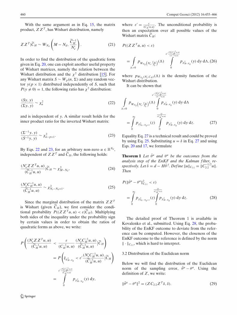
460 Comput Geosci (2012) 16:455–466

With the same argument as in Eq. 15, the matrixproduct, Z Z T , has Wishart distribution, namely

Z Z T |C̃H ∼ WNd

(

M − Nd,C̃−1

H

N′e

)

. (21)

In order to find the distribution of the quadratic formgiven in Eq. 20, one can exploit another useful propertyof Wishart matrices, namely the relation between theWishart distribution and the χ2 distribution [15]. Forany Wishart matrix S ∼ Wp(n, �) and any random vec-tor y(p × 1) distributed independently of S, such thatP(y = 0) = 1, the following ratio has χ2 distribution:

(Sy, y)

(�y, y)∼ χ2

n (22)

and is independent of y. A similar result holds for theinner product ratio for the inverted Wishart matrix:

(�−1 y, y)

(S−1 y, y)∼ χ2

n−p+1. (23)

By Eqs. 22 and 23, for an arbitrary non-zero u ∈ RNd ,

independent of Z Z T and C̃H , the following holds:

(N′e Z Z Tu, u)

(C̃−1H u, u)

|C̃H ∼ χ2M−Nd

, (24)

(N′eC−1

H u, u)

(C̃−1H u, u)

∼ χ2Ne−Nd+1. (25)

Since the marginal distribution of the matrix Z Z T

is Wishart (given C̃H), we first consider the condi-tional probability P((Z Z Tu, u) < ε|C̃H). Multiplyingboth sides of the inequality under the probability signby certain values in order to obtain the ratios ofquadratic forms as above, we write:

P

((N′

e Z Z Tu, u)

(C̃−1H u, u)

<ε

(C−1H u, u)

(N′eC−1

H u, u)

(C̃−1H u, u)

∣∣C̃H

)

= P

(

ξχ2M−Nd

< ε′ (N′eC−1

H u, u)

(C̃−1H u, u)

∣∣C̃H

)

=ε′ (N′

eC−1H u,u)

(C̃−1H u,u)∫

0

pχ2M−Nd

(y) dy,

where ε′ = ε

(C−1H u,u)

. The unconditional probability is

then an expectation over all possible values of theWishart matrix C̃H :

P((Z Z Tu, u) < ε)

=∫

>0

pWNd

(N′

e,CHN′

e

)()

ε′ (N′eC−1

H u,u)

(−1u,u)∫

0

pχ2M−Nd

(y) dy d,(26)

where pWNd (N′e,CH)() is the density function of the

Wishart distribution.It can be shown that

∫

>0

pWNd

(N′

e,CHN′

e

)()

ε′ (N′eC−1

H u,u)

(−1u,u)∫

0

pχ2M−Nd

(y) dy d

=∞∫

0

pχ2Ne−Nd+1

(z)

zε

(C−1H u,u)∫

0

pχ2M−Nd

(y) dy dz. (27)

Equality Eq. 27 is a technical result and could be provedby using Eq. 25. Substituting u = δ in Eq. 27 and usingEqs. 20 and 17, we formulate

Theorem 1 Let θ̄a and θa be the outcomes from theanalysis step of the EnKF and the Kalman f ilter, re-spectively. Let δ = d − Hθ̄ f . Def ine ‖u‖C2·2 = ‖C−1/2

2·2 u‖.Then

P(‖θ̄a − θa‖2C2·2 < ε)

=∞∫

0

pχ2Ne−Nd+1

(z)

zε

(C−1H δ,δ)∫

0

pχ2M−Nd

(y) dy dz. (28)

The detailed proof of Theorem 1 is available inKovalenko et al., submitted. Using Eq. 28, the proba-bility of the EnKF outcome to deviate from the refer-ence can be computed. However, the closeness of theEnKF outcome to the reference is defined by the norm‖ · ‖C2·2 , which is hard to interpret.

3.2 Distribution of the Euclidean norm

Below we will find the distribution of the Euclideannorm of the sampling error, θ̄a − θa. Using thedefinition of Z , we write:

‖θ̄a − θa‖2 = (ZC2·2 Z Tδ, δ). (29)

Comput Geosci (2012) 16:455–466 461

In order to derive the distribution for the latter norm,we consider the following decomposition of the matrixC2·2:

C2·2 = σ 21 P1 + · · · + σ 2

M−NdPM−Nd, (30)

where σi is a singular value of C2·2 and Pi is a corre-sponding projection matrix [16]. Such a decompositionis called a spectral decomposition of a symmetric ma-trix, and the decomposition is unique. For the sake ofsimplicity, we will consider the case when the matrixC2·2 has unequal singular values, and the correspondingprojection matrices are all of rank 1. A similar resultfor the general case is easily obtained by following thesame proof with minor adjustments.

Applying the spectral decomposition to the matrix inthe inner product in Eq. 29, we get:

(ZC2·2 Z Tδ, δ)

=M−Nd∑

i=1

σ 2i (Z Pi Z Tδ, δ) =

M−Nd∑

i=1

σ 2i (Z P2

i Z Tδ, δ) =

=M−Nd∑

i=1

σ 2i (Pi Z Tδ, Pi Z Tδ). (31)

Since Pi P j = 0, i = j, the sum terms in Eq. 31 areindependent, and we will consider the distribution ofa single inner product, (Pi Z Tδ, Pi Z Tδ), thus findingthe distribution for the norm of the sampling error.Since Z |C̃H is a normally distributed matrix, we useEq. 13 setting D = δT and write the following marginaldistribution for the random vector Pi Z Tδ:

Pi Z Tδ|C̃H ∼ N(

0,(C̃−1

H δ, δ)

N′e

× P2i

)

.

Normalizing the variance, we obtain:√

N′e

(C̃−1H δ, δ)1/2

Pi Z Tδ|C̃−1H ∼ N (0, P2

i ).

Denote v =√

N′e

(C̃Hδ,δ)1/2 Pi Z Tδ. Since rank Pi < M −Nd, the vector has a singular multivariate normal dis-tribution. There exists a unique orthogonal matrix Qi

for each of the projectors Pi such that

Qi P2i QT

i =

⎛

⎜⎜⎜⎝

1 0 · · · 00 0 · · · 0...

.... . .

...

0 0 · · · 0

⎞

⎟⎟⎟⎠

,

and Qi QTi = I [17]. Applying this transform to the

vector, we obtain:

Qiv|C̃H ∼ N (0, Qi P2i QT

i ).

Denote the resulting covariance, Qi P2i QT

i = Li. Notethat Li is a symmetric projection matrix, and Li =Li LT

i .By definition of the multivariate normal distribution,

a normally distributed vector u ∼ N (μ, G) can be writ-ten as u = μ + Rζ , where ζ ∼ N (0, I) and RRT = G.Since Qi P2

i QTi = Li LT

i = Li, we write for the resultingvector, Qiv:

Qiv = Qi P2i QT

i

⎛

⎜⎜⎜⎝

ξ1

ξ2...

ξM−Nd

⎞

⎟⎟⎟⎠

=

⎛

⎜⎜⎜⎝

ξ1

0...

0

⎞

⎟⎟⎟⎠

,

where ξk|C̃H ∼ N (0, 1), k = 1, . . . , M − Nd. The innerproduct (v, v) is then

(v, v) = (QTi Qiv, v) = (Qiv, Qiv)

= (ξ1, 0, . . . , 0)

⎛

⎜⎜⎜⎝

ξ1

0...

0

⎞

⎟⎟⎟⎠

= ξ 21 .

Since ξ1 is marginally normal, the ith term of the sumhas a marginal χ2

1 distribution:

N′e(Pi Z Tδ, Pi Z Tδ)

(C̃−1H δ, δ)

|C̃H ∼ χ21 . (32)

After dividing by (C̃−1H δ,δ)

N′e

, the sum in Eq. 31 becomes

N′e

(C̃−1H δ, δ)

M−Nd∑

i=1

σ 2i (Pi Z Tδ, Pi Z Tδ)

= N′e

(C̃−1H δ, δ)

M−Nd∑

i=1

σ 2i χ2

1 .

We will call the weighted sum of the squared standardnormal variables a generalized χ2 distribution denotedas χ2

C2·2 , with corresponding density function pχ2C2·2

. Re-placing the marginal distribution of the squared energynorm in Eq. 24 with the obtained distribution andusing representation 22, we write for the conditionaldistribution, P(‖θ̄a − θa‖2 < ε|C̃H):

P

((N′

e ZC2·2 Z Tδ, δ)

(C̃−1H δ, δ)

< ε′ (N′eC−1

H δ, δ)

(C̃−1H δ, δ)

∣∣C̃H

)

= P

(

ξχ2C2·2

< ε′ (N′eC−1

H δ, δ)

(C̃−1H δ, δ)

∣∣C̃H

)

=ε′ (N′

eC−1H δ,δ)

(C̃−1H δ,δ)∫

0

pχ2C2·2

(y) dy,

where ε′ = ε

(C−1H δ,δ)

and ξχ2C2·2

denotes the random value

having a generalized χ2 distribution.

462 Comput Geosci (2012) 16:455–466

Integrating over all C̃H as in Eq. 26 and simplifyingthe resulting integral as in Eq. 27, we may now refor-mulate Theorem 1 for the regular Euclidean norm.

Theorem 2 Let θ̄a and θa be the outcomes from theanalysis step of the EnKF and the Kalman f ilter respec-tively. Let δ = d − Hθ̄ f . Then

P(‖θ̄a − θa‖2 < ε)

=∞∫

0

pχ2Ne−Nd+1

(z)

zε

(C−1H δ,δ)∫

0

pχ2C2·2

(y) dy dz. (33)

By utilizing the distribution for the Euclidean normof the sampling error, the behavior of the EnKF canbe more easily assessed. Computing the double integralin Eq. 33 is a little more elaborate in comparison withEq. 28 because of the generalized χ2 distribution in-volved, but the computational effort is comparable.For reference on computation of the generalized χ2

distribution, see, e.g., [5].

4 Numerical experiments

In this section, we demonstrate how Theorem 2 can beused to assess the reliability of EnKF. We assume thatthe result of the forecast stage is Gaussian in order tofulfill the requirements of Theorem 2. That is, we donot consider the additional difficulties the EnKF mightencounter if the forecast distribution is not Gaussian.

We will investigate the effect of the numerical pa-rameters included in the distribution 33, such as thesystem size, M, the number of ensemble members,Ne, and the number of observations, Nd. We will alsoinvestigate the effect of changing the structure of theobservation operator, H.

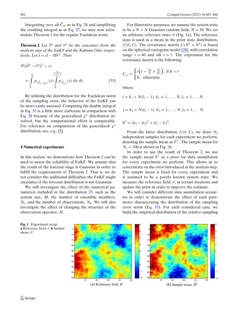
For illustrative purposes, we assume the system stateto be a N × N Gaussian random field, N = 50. We setan arbitrary reference state, θ (Fig. 1a). The referencestate is used as a mean in the prior state distribution,N (θ, C). The covariance matrix C(N2 × N2) is basedon the spherical variogram model [28], with correlationrange r = 40 and sill s = 1. The expression for thecovariance matrix is the following:

Ci, j ={

s(

1 − 3h2r + h3

2r3

), if h < r

0, otherwise,

where

i = k1 + N(l1 − 1), k1 = 1, . . . , N, l1 = 1, . . . N,

j = k2 + N(l2 − 1), k2 = 1, . . . , N, l2 = 1, . . . N,

h2 = (k1 − k2)2 + (l1 − l2)

2.

From the latter distribution N (θ, C), we draw Ne

independent samples for each experiment we perform,denoting the sample mean as θ̄ f . The sample mean forNe = 100 is shown in Fig. 1b.

In order to use the result of Theorem 2, we usethe sample mean θ̄ f as a prior for data assimilationfor every experiment we perform. This allows us toconcentrate on the error introduced at the analysis step.The sample mean is fixed for every experiment andis assumed to be a poorly known system state. Wemeasure the reference field, θ , at certain locations andupdate the prior in order to improve the estimate.

We will consider different data assimilation scenar-ios in order to demonstrate the effect of each para-meter characterizing the distribution of the samplingerror norm (Eq. 33). For each considered case, webuild the empirical distribution of the relative sampling

Fig. 1 Experiment setup.a Reference field, θ . b Samplemean, θ̄ f

10 20 30 40 50

5

10

15

20

25

30

35

40

45

50 −2

−1

0

1

2

3

4

5

6

(a) Reference field, θ

10 20 30 40 50

5

10

15

20

25

30

35

40

45

50 −2

−1

0

1

2

3

4

5

6

(b) Sample mean, −θ f

Comput Geosci (2012) 16:455–466 463

error, ‖θ̄a − θa‖/‖θ̄ f ‖. We use 50 points to build theempirical distribution. For this, we generate 50 inde-pendent realizations of the sample covariance matrix.Each realization is a sample drawn from the Wishartdistribution, WM(N′

e,CN′

e). Each of the 50 matrices is

then used in Eqs. 10–11, and the sampling error norm iscalculated using Eq. 17, divided then by ‖θ̄ f ‖. Resultingvalues of the sampling error norm are then used to plotthe empirical distribution. Even though 50 empiricalrealizations of the sampling error norm is relatively few,the number is sufficient for illustrative purposes, such

that empirical and analytical distributions can easily bedistinguished.

The analytical expression for the sampling errorgiven in Theorem 2 is compared with the empiricaldistribution. For a given measurement layout and cor-responding matrix H, we calculate the quadratic form(C−1

H δ, δ) and use formula 33, thus building the cumu-lative distribution function for the squared samplingerror ‖θ̄a − θa‖2. A simple variable transform in Eq. 33gives the distribution for the relative sampling error,‖θ̄a − θa‖/‖θ̄ f ‖.

Fig. 2 Distribution of theerror norm, Ne − Nd = 50.a Measurements locations,Nd = 10. b Sampling errordistribution, Ne = 60.c Measurements locations,Nd = 20. d Sampling errordistribution, Ne = 70.e Measurements locations,Nd = 40. f Sampling errordistribution, Ne = 90

5 10 15 20 25 30 35 40 45 50

5

10

15

20

25

30

35

40

45

50

(a) Measurements locations, Nd = 10

0 0.1 0.2 0.3 0.4 0.5 0.6 0.70

0.1

0.2

0.3

0.4

0.5

0.6

0.7

0.8

0.9

1P

(b) Sampling error distribution, Ne = 60

5 10 15 20 25 30 35 40 45 50

5

10

15

20

25

30

35

40

45

50

(c) Measurements locations, Nd = 20

0 0.1 0.2 0.3 0.4 0.5 0.6 0.70

0.1

0.2

0.3

0.4

0.5

0.6

0.7

0.8

0.9

1P

(d) Sampling error distribution, Ne = 70

5 10 15 20 25 30 35 40 45 50

5

10

15

20

25

30

35

40

45

50

(e) Measurements locations, Nd = 40

0 0.1 0.2 0.3 0.4 0.5 0.6 0.70

0.1

0.2

0.3

0.4

0.5

0.6

0.7

0.8

0.9

1P

(f) Sampling error distribution, Ne = 90

464 Comput Geosci (2012) 16:455–466

4.1 Experiment 1

In this section, we consider the case when Ne − Nd isconstant and equal to 50. For this purpose, we varyM − Nd by varying the number of measurements and,correspondingly, the ensemble size. We concentrate themeasurement locations at the upper left corner of thefield.

The figures on the left-hand side (Fig. 2a, c, e) il-lustrate the measurement locations, while the figures

on the right-hand side (Fig. 2b, d, f) display the cor-responding error distributions. The solid blue line cor-responds to the cumulative distribution function of therelative sampling error, and the dashed red line is theempirical distribution for the same variable.

As seen from the resulting distributions, increasingthe number of measurement locations leads to increaseof the sampling error despite the increase of the ensem-ble size. The effect seen in this experiment arises dueto changes in spectral properties of both CH and C2·2

Fig. 3 Distribution of theerror norm, M − Nd =2460, Ne − Nd = 50, variedmeasurement locations. aMeasurements locations,dense layout. b Samplingerror distribution, denselayout. c Measurementslocations, wide layout. dSampling error distribution,wider layout. e Measurementslocations, spread layout. fSampling error distribution,spread layout

5 10 15 20 25 30 35 40 45 50

5

10

15

20

25

30

35

40

45

50

(a) Measurements locations, dense layout

0 0.1 0.2 0.3 0.4 0.5 0.6 0.70

0.1

0.2

0.3

0.4

0.5

0.6

0.7

0.8

0.9

1P

(b) Sampling error distribution, dense layout

5 10 15 20 25 30 35 40 45 50

5

10

15

20

25

30

35

40

45

50

(c) Measurements locations, wide layout

0 0.1 0.2 0.3 0.4 0.5 0.6 0.70

0.1

0.2

0.3

0.4

0.5

0.6

0.7

0.8

0.9

1P

(d) Sampling error distribution, wider layout

5 10 15 20 25 30 35 40 45 50

5

10

15

20

25

30

35

40

45

50

(e) Measurements locations, spread layout

0 0.1 0.2 0.3 0.4 0.5 0.6 0.70

0.1

0.2

0.3

0.4

0.5

0.6

0.7

0.8

0.9

1P

(f) Sampling error distribution, spread layout

Comput Geosci (2012) 16:455–466 465

matrices, when increasing the number of the measure-ments, see Eq. 33.

4.2 Experiment 2

In this experiment, we consider a fixed ensemble size,Ne = 90, and a fixed number of measurements, Nd =40. Since M is constant, M − Nd is also constant. Wevary the locations of the measurements and build thecorresponding distributions.

As before, the left-hand side plots in Fig. 3 showthe measurement layouts, and the plots on the oppositedemonstrate the corresponding distributions. As seenfrom the figures, spreading the measurements acrossthe field implies a smaller sampling error. Since we varythe structure of the measurement matrix, H, the matri-ces C2·2 and C−1

H vary correspondingly. The singular val-ues of C2·2 and the matrix C−1

H are the only parametersaffecting the sampling error norm distribution in thisexperiment. Thus, the spreading of the measurementsimproves both spectral properties of the C2·2 matrix andthe condition number of the matrix CH , making theresult of the EnKF analysis step a better estimate.

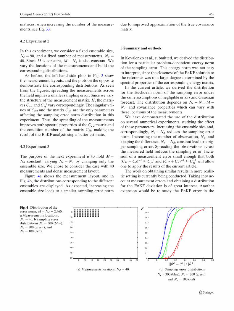
4.3 Experiment 3

The purpose of the next experiment is to hold M −Nd constant, varying Ne − Nd by changing only theensemble size. We chose to consider the case with 40measurements and dense measurement layout.

Figure 4a shows the measurement layout, and inFig. 4b, the distributions corresponding to the differentensembles are displayed. As expected, increasing theensemble size leads to a smaller sampling error norm

due to improved approximation of the true covariancematrix.

5 Summary and outlook

In Kovalenko et al., submitted, we derived the distribu-tion for a particular problem-dependent energy normof the sampling error. This energy norm was not easyto interpret, since the closeness of the EnKF solution tothe reference was to a large degree determined by thespectral properties of the corresponding energy matrix.

In the current article, we derived the distributionfor the Euclidean norm of the sampling error underthe same assumptions of negligible errors and Gaussianforecast. The distribution depends on Ne − Nd, M −Nd, and covariance properties which can vary withthese locations of the measurements.

We have demonstrated the use of the distributionon several numerical experiments, studying the effectof these parameters. Increasing the ensemble size and,correspondingly, Ne − Nd reduces the sampling errornorm. Increasing the number of observation, Nd, andkeeping the difference, Ne − Nd, constant lead to a big-ger sampling error. Spreading the observations acrossthe measured field reduces the sampling error. Inclu-sion of a measurement error small enough that both(CH + Cd)

−1 ≈ C−1H and (C̃H + Cd)

−1 ≈ C̃−1H will allow

one to apply the results of the current article.The work on obtaining similar results in more realis-

tic setting is currently being conducted. Taking into ac-count measurement errors and obtaining a distributionfor the EnKF deviation is of great interest. Anotherextension would be to study the EnKF error in the

Fig. 4 Distribution of theerror norm, M − Nd = 2,460.a Measurements locations,Nd = 40. b Sampling errordistributions Ne = 300 (blue),Ne = 200 (green), andNe = 100 (red)

5 10 15 20 25 30 35 40 45 50

5

10

15

20

25

30

35

40

45

500 0.1 0.2 0.3 0.4 0.5 0.6 0.7

0

0.1

0.2

0.3

0.4

0.5

0.6

0.7

0.8

0.9

1P

(a) Measurements locations, Nd = 40 (b) Sampling error distributions

Ne = 300 (blue), Ne = 200 (green)

and Ne = 100 (red)

466 Comput Geosci (2012) 16:455–466

case of several time steps. Such results will significantlyimprove the understanding of the EnKF reliability inapplications.

Acknowledgements The authors would like to acknowledgefinancial support to perform this study from the Research Coun-cil of Norway (Petromaks), Rocksource, Statoil, and Total.

Open Access This article is distributed under the terms of theCreative Commons Attribution Noncommercial License whichpermits any noncommercial use, distribution, and reproductionin any medium, provided the original author(s) and source arecredited.

References

1. Aanonsen, S.I., Aavatsmark, I., Barkve, T., Cominelli, A.,Gonard, R., Gosselin, O., Kolasinski, M., Reme, H.: Effectof scale dependent data correlations in an integrated historymatching loop combining production data and 4D seismicdata. In: Proc. SPE Reservoir Simulation Symposium, paperSPE 79665. Houston, Texas (2003)

2. Aanonsen, S.I., Nævdal, G., Oliver, D.S., Reynolds, A.C.,Valles, B.: The ensemble Kalman filter in reservoirengineering—a review. SPE J. 14(3), 393–412 (2009)

3. Bennett, A.F.: Inverse Modeling of the Ocean and At-mosphere. Cambridge University Press, Cambridge (2002)

4. Chen, C., Wang, Y., Li, G., Reynolds, A.: Closed-loop reser-voir management on the Brugge test case. ComputationalGeosciences 14, 691–703 (2010)

5. Davies, R.B.: Algorithm as 155: the distribution of a linearcombination of χ2 random variables. J. R. Stat. Soc., Ser. C,Appl. Stat. 29(3), 323–333 (1980)

6. Dong, Y., Oliver, D.S.: Quantitative use of 4D seismic datafor reservoir description. SPE J. 10(1), 91–99 (2005)

7. Evensen, G.: Sequential data assimilation with a nonlin-ear quasi-geostrophic model using Monte Carlo methods toforecast error statistics. J. Geophys. Res. 99, 10143–10162(1994)

8. Evensen, G.: The ensemble Kalman filter: theoretical formu-lation and practical implementation. Ocean Dyn. 53, 343–367(2003)

9. Evensen, G.: Sampling strategies and square root analysisschemes for the EnKF. Ocean Dyn. 54, 539–560 (2004)

10. Evensen, G.: Data Assimilation: The Ensemble Kalman Fil-ter, 2nd edn. Springer, New York (2009)

11. Evensen, G., van Leeuwen, P.J.: An ensemble Kalmansmoother for nonlinear dynamics. Mon. Weather Rev. 128(6),1852–1867 (2000)

12. Fahimuddin, A., Mannseth, T., Aanonsen, S.I.: Effect oflarge number of measurements on the performance of EnKFmodel updating. In: Proceedings of the 11th European Con-ference on the Mathematics of Oil Recovery (ECMOR XI).Bergen, Norway (2008)

13. Feng, T., Mannseth, T.: Impact of time-lapse seismic data forpermeability estimation. Comput. Geosci. 14, 705–719 (2010)

14. Furrer, R., Bengtsson, T.: Estimation of high-dimensionalprior and posterior covariance matrices in Kalman filter vari-ants. J. Multivar. Anal. 98(2), 227–255 (2007)

15. Gupta, A.K., Nagar, D.K.: Matrix variate distributions.Chapman & Hall/CRC Monographs and Surveys in Pure andApplied Mathematics, vol. 104. Chapman & Hall/CRC, BocaRaton (2000)

16. Hayakawa, T.: On the distribution of a quadratic form in amultivariate normal sample. Ann. Inst. Stat. Math. 18, 191–201 (1966)

17. Horn, R.A., Johnson, C.R.: Matrix Analysis. Cambridge Uni-versity Press, Cambridge (1990)

18. Houtekamer, P.L., Mitchell, H.L.: Data assimilation usingan ensemble Kalman filter technique. Mon. Weather Rev.126(3), 796–811 (1998)

19. Kalman, R.E.: A new approach to linear filtering and pre-diction problems. Trans. Am. Soc. Mech. Eng.–J. Basic Eng.82(Series D), 35–45 (1960)

20. Kepert, J.D.: On ensemble representation of the observation-error covariance in the ensemble Kalman filter. Ocean Dyn.54, 561–569 (2004)

21. Kovalenko, A., Mannseth, T., Nævdal, G.: Error estimate forthe ensemble Kalman filter update step. In: Proceedings ofthe 12th European Conference on the Mathematics of OilRecovery (ECMOR XII). Oxford, UK (2010)

22. Nævdal, G., Johnsen, L.M., Aanonsen, S.I., Vefring, E.H.:Reservoir monitoring and continuous model updating usingensemble Kalman filter. SPE J. 10(1), 66–74 (2005)

23. Nævdal, G., Mannseth, T., Vefring, E.H.: Near-well reservoirmonitoring through ensemble Kalman filter. In: The 2002SPE/DOE Improved Oil Recovery Symposium, Paper SPE75235. Tulsa, Oklahoma (2002)

24. Oliver, D., Chen, Y.: Ensemble-based closed-loop optimiza-tion applied to Brugge field. SPE Reserv. Evalu. Eng. 13(1),56–71 (2010)

25. Oliver, D., Chen, Y.: Recent progress on reservoir historymatching: a review. Comput. Geosci. 15, 1–37 (2010)

26. Skjervheim, J.A., Evensen, G., Aanonsen, S.I., Ruud, B.O.,Johansen, T.A.: Incorporating 4D seismic data in reservoirsimulation models using ensemble Kalman filter. SPE J.12(3), 282–292 (2007)

27. Srivastava, M.S.: Singular Wishart and multivariate beta dis-tributions. Ann. Stat. 31(5), 1537–1560 (2003)

28. Wackernagel, H., Bertino, L.: Geostatistics and SequentialData Assimilation. Springer, New York (2005)