Establishing Global Error Bounds for Model Reduction in ...

Establishing Global Error Bounds for Model

Reduction in Combustion

by ARCHES

Geoffrey Malcolm Oxberry OFTECHNOLOGY

B. Ch. E., University of Delaware (2006) LM. Ch. E., University of Delaware (2006) LIBA

Submitted to the Department of Chemical Engineering

in partial fulfillment of the requirements for the degree of

Doctor of Philosophy in Chemical Engineering

at the

MASSACHUSETTS INSTITUTE OF TECHNOLOGY

February 2013

© Massachusetts Institute of Technology 2013. All rights reserved.

A u th or ........ ... . ..... ........ ..... .......................Depuhment of Chemical Engineering

September 26, 2012

Certified by . ...................Paul I. Barton

Lammot du Pont Professor of Chemical EngineeringThesis Supervisor

C ertified by ....... .............................William H. Green

Hoyt C. Hottel Professor of Chemical EngineeringThesis Supervisor

A ccepted by .......... ..........................Patrick S. Doyle

Chairman, Committee on Graduate Students

MIT LibrariesDocument Services

Room 14-055177 Massachusetts AvenueCambridge, MA 02139Ph: 617.253.2800Email: [email protected]://Iibraries.mit.edu/docs

DISCLAIMER OF QUALITY

Due to the condition of the original material, there are unavoidableflaws in this reproduction. We have made every effort possible toprovide you with the best copy available. If you are dissatisfied withthis product and find it unusable, please contact Document Services assoon as possible.

Thank you.

Some pages in the original document contain text thatruns off the edge of the page.

Establishing Global Error Bounds for Model Reduction in

Combustion

by

Geoffrey Malcolm Oxberry

Submitted to the Department of Chemical Engineeringon September 26, 2012, in partial fulfillment of the

requirements for the degree ofDoctor of Philosophy in Chemical Engineering

Abstract

In addition to theory and experiment, simulation of reacting flows has become im-portant in policymaking, industry, and combustion science. However, simulationsof reacting flows can be extremely computationally demanding due to the widerange of length scales involved in turbulence, the wide range of time scales in-volved in chemical reactions, and the large number of species in detailed chemicalreaction mechanisms in combustion. To compensate for limited available com-putational resources, reduced chemistry is used. However, the accuracy of thesereduced chemistry models is usually unknown, which is of great concern in appli-cations; if the accuracy of a simplified model is unknown, it is risky to rely on theresults of that model for critical decision-making.

To address this issue, this thesis derives bounds on the global error in reducedchemistry models. First, it is shown that many model reduction methods in com-bustion are based on projection; all of these methods can be described using thesame equation. After that, methods from the numerical solution of ODEs are usedto derive separate a priori bounds on the global error in the solutions of reducedchemistry models for both projection-based reduced chemistry models and non-projection-based reduced chemistry models. The distinguishing feature betweenthe two sets of bounds is that bounds on projection-based reduced chemistry mod-els are stronger than those on non-projection-based reduced chemistry models. Inboth cases, the bounds are tight, but tend to drastically overestimate the error inthe reduced chemistry. The a priori bounds on the global error in the solutions ofreduced chemistry models demonstrate that if the error in the time derivatives ofthe state variables in the reduced model is controlled, then the error in the reducedmodel solution is also controlled; this thesis proves that result for the first time.Source code is included for all results presented.

After presenting these results, the development of more accurate global errorinformation is discussed. Using the error bounds above, in concert with moreaccurate global error information, it should be possible to assess better the accuracy

3

and reliability of reduced chemistry models in applications.

Thesis Supervisor: Paul I. BartonTitle: Lammot du Pont Professor of Chemical Engineering

Thesis Supervisor: William H. GreenTitle: Hoyt C. Hottel Professor of Chemical Engineering

4

Look at us. Look at what they make

you give.

Jason Bourne, The Bourne

Ultimatum

5

Acknowledgments

First, I would like to thank my parents, Brett and Kathleen, and my siblings,

Mallory and Matthew, for their support over the course of my PhD. Without my

mother's support, I certainly would not have been able to finish.

Second, I would like to thank my advisers, Prof. Paul I. Barton and Prof. William

H. Green, for their advice and support. Professor Green has been a great resource

in helping me understand the broader implications of my research, and helping

me navigate the PhD process. Professor Barton has been instrumental in helping

me better articulate my ideas. Both men are brilliant researchers, and I would not

have been able to finish this thesis without them.

Third, I would like to thank the Department of Energy (DOE) Computational

Science Graduate Fellowship (CSGF) program and the Krell Institute staff, espe-

cially Dr. Mary Ann Leung, Jeana Gingery, Michelle King, and Jim Corones, for

all of their support and guidance during my PhD thesis. In addition to provid-

ing me with four years of very generous financial support, the DOE CSGF alumni

(and their friends) have taught me countless lessons in what it means to be a com-

putational scientist. In particular, Dr. Jaydeep Bardhan and Dr. Ahmed E. Ismail

have been great career mentors and have helped me understand how to be a bet-

ter scientist and human being. I would also like to thank Dr. Aron Ahmadia his

insight and guidance regarding the Python programming language, and to Ethan

Coon and countless other CSGFers who have promoted the language. Their in-

fluence on the implementation of the examples presented in this thesis will be

evident to anyone who reads it. I would like to thank Dr. David Ketcheson for

his comments on Chapters 3 and 4 of this thesis, because he provided the most

valuable conceptual edits for this entire manuscript. Dr. Jed Brown, for me, will

always be a role model for the breadth of mathematical techniques he has mas-

tered, spanning several branches of the numerical solution of partial differential

equations and numerical linear algebra, as well as for his programming (and rock-

climbing) skill. He has been a great sounding board when it comes to tackling

7

some of the algorithmic tasks I faced over the course of this thesis. I'd like to thank

Dr. Jeff Hammond and Dr. Chris Rinderspacher for very lively discussions about

computational science over the course of my thesis, and Dr. Matt Reuter for his

camaraderie and great physical insight. In addition to all of the networking that

the DOE CSGF program provided, and countless talks about computational sci-

ence from staff scientists at the national labs and from CSGF alumni, I believe that

being an alumnus helped me get a job at a national laboratory. Technical service in

the national interest has always been a dream of mine, since I would like to give

back to the community of people who helped me get to where I am today.

Fourth, I'd like to thank the staff of MIT Medical, especially Araceli Isenia, Dr.

Sherry Bauman, and Dr. Jill Colman. Over the course of my thesis, I encountered

a few serious medical issues, and without their help, I definitely would not have

been able to finish. I wish them the best of luck with their future endeavors.

In addition, I'd like to thank several colleagues in the Barton and Green groups

for their help and support. Dr. Ray Speth's work on Cantera was instrumental to

helping me open-source the implementations of the examples in my thesis, and

I look forward to working with him to contribute to Cantera in the future. Dr.

Richard West, Josh Allen, and the rest of the RMG team have been an excellent

example of what computational scientists should be doing when developing soft-

ware; in particular, I would like to thank Dr. West for helping to convince people

in the group to use Python and Git. In the Barton group, I'd like to thank Achim

Wechsung, Spencer Schaber, and Matt Stuber for a lot of engaging conversations.

I wish you all the best of luck in your future careers.

Finally, I'd like to thank my friends for helping me get out of the lab and

relax (if only a little), particularly Ben Rosehart, Stephanie Anton, Jess Martin,

Colleen Dunn, Jess Cochrane, Nicole Romano, Christine Tinker, Christy Petruczok

(for keeping me sane), Kristin Vicari (for inviting me to my first Red Sox-Yankees

game), and Rachel Howden (especially for organizing all of the social events).

8

This doctoral thesis has been examined by a Committee of theDepartment of Chemical Engineering as follows:

Professor William M. Deen .. ............................Chairman, Thesis Committee

Carbon P. Dubbs Professor of Chemical Engineering

Professor Paul I. Barton ............................................Thesis Supervisor

Lammot du Pont Professor of Chemical Engineering

Professor W illiam H. Green ........................................Thesis Supervisor

Hoyt C. Hottel Professor of Chemical Engineering

Professor M artin Z. Bazant.........................................Member, Thesis Committee

Professor of Chemical Engineering

Contents

1 Introduction 19

2 Projection-Based Model Reduction in Combustion 25

2.1 Introduction . . . . . . . . . . . . . . . . . . . . . . . . . . . . . . . . . 25

2.2 Defining "Projection-Based Model Reduction Method" . . . . . . . . 28

2.3 Three Representations of Constant Projection-Based Model Reduction 30

2.3.1 Projector Representation . . . . . . . . . . . . . . . . . . . . . . 30

2.3.2 Affine Lumping/Petrov-Galerkin Projection Representation . 34

2.3.3 Affine Invariant/Linear Manifold Representation . . . . . . . 41

2.4 Examples of Projection-Based Model Reduction Methods . . . . . . . 46

2.4.1 Projector Representation . . . . . . . . . . . . . . . . . . . . . . 46

2.4.2 Affine Lumping/Petrov-Galerkin Projection Representation . 48

2.4.3 Affine Invariant Representation . . . . . . . . . . . . . . . . . . 51

2.5 D iscussion . . . . . . . . . . . . . . . . . . . . . . . . . . . . . . . . . . 54

2.6 Conclusions . . . . . . . . . . . . . . . . . . . . . . . . . . . . . . . . . 55

3 State-Space Error Bounds For Projection-Based Reduced Model ODEs 57

3.1 Introduction . . . . . . . . . . . . . . . . . . . . . . . . . . . . . . . . . 57

3.2 Projection-Based Model Reduction . . . . . . . . . . . . . . . . . . . . 59

3.3 Mathematical Preliminaries . . . . . . . . . . . . . . . . . . . . . . . . 61

3.4 Error Analysis for Projection-Based Model Reduction . . . . . . . . . 63

3.5 Case Study . . . . . . . . . . . . . . . . . . . . . . . . . . . . . . . . . . 74

3.6 D iscussion . . . . . . . . . . . . . . . . . . . . . . . . . . . . . . . . . . 81

11

3.7 Conclusions and Future Work ............................ 84

4 State-Space Error Bounds For All Reduced Model ODEs

4.1 Introduction . . . . . . . . . . . . . . . . . . . . . . .

4.2 Model Reduction ........................

4.3 Mathematical Preliminaries ................

4.4 Error Analysis for Model Reduction . . . . . . . . .

4.5 Case Study . . . . . . . . . . . . . . . . . . . . . . . .

4.6 D iscussion . . . . . . . . . . . . . . . . . . . . . . . .

4.7 Conclusions and Future Work .............

87

. . . . . . . . . . 87

. . . . . . . . . . 88

. . . . . . . . . . 90

. . . . . . . . . . 92

. . . . . . . . . . 98

. . . . . . . . . . 103

. . . . . . . . . . 104

5 Contributions and Future Work

5.1 Contributions . . . . . . . . . . . . . . . . . . . . . . . . . . . . . . .

5.2 Future W ork . . . . . . . . . . . . . . . . . . . . . . . . . . . . . . . .

5.2.1 Opportunities to Develop New Model Reduction Methods .

5.2.2 Opportunities to Develop Better Error Estimates and Bounds

A Implementation of Examples for Chapter 2

A.1 Cantera Ozone CTI file ..........

A.2 MATLAB Implementation .........

A.3 Python Implementation .........

B Implementation of Examples for Chapter 3

B.1 MATLAB Implementation .........

B.2 Python Implementation .........

C Implementation of Examples for Chapter 4

C.1 MATLAB Implementation .........

C.2 Python Implementation .........

D Implementation of Point-Constrained Reaction Elimination and Point-

Constrained Simultaneous Reaction and Species Elimination Formula-

12

105

105

106

107

116

119

119

121

133

173

173

183

199

199

203

tions in Chapter 5 209

D.1 Python Implementation .......................... 209

D.2 Python Unit Tests .............................. 217

13

List of Figures

2-1 Graphical depiction of projector representation for adiabatic 03 de-

composition. Here, the model is reduced from 3 variables to 2 by

projecting orthogonally onto the plane shown. The resulting re-

duced model solution is a line, due to mass conservation. . . . . . . . 32

2-2 Two examples illustrating the decomposition of a vector into com-

ponents along the range and nullspace of a projection matrix P. In

the orthogonal case, P = pT. . . . . . . . . . . . . . . . . . . . . . . . 33

2-3 Graphical depiction of Petrov-Galerkin/affine lumping representa-

tion for the same adiabatic 03 decomposition in Figure 2-1. Here,

the lumped variable is on the x-axis, and is an affine combination of

the mass fractions of 0, 02 and 03; the coefficients of this relation-

ship are the first column of V in (2.23). Note that yo is the lowermost

point of both curves in the lower left-hand corner; the sharp bend

in the upper left-corner indicates that the mass fraction of 0 and

lumped variable have both achieved steady state. . . . . . . . . . . . 38

2-4 Graphical depictions of affine invariant representation for adiabatic

03 decomposition; note that this case is different than those in Fig-

ures 2-1 and 2-3 in order to yield a more illustrative plot. Here, the

mass fraction of 02 is held constant at y0 2 = 6.83252318. 10-1, and

the point yo is the intersection of the two curves, found lower right.

The sharp bend in the plot corresponds to the establishment of 03 =

02 + 0 equilibrium . . . . . . . . . . . . . . . . . . . . . . . . . . . . . . 45

15

3-1 Illustrates the relationships among the full model solution y, the

projected solution ' (see (3.22)), the reduced model solution x, and

the error e. Note that the error is decomposed into a component in

R(P) denoted ei, and a component in JM(P) denoted ec. . . . . . . . . 65

3-2 First three components of x(t) (dashed) and y(t) (solid) correspond-

ing to the first choice of A as in (3.49), (3.50), (3.51), (3.52), and (3.53)

and its corresponding projector. . . . . . . . . . . . . . . . . . . . . . . 77

3-3 Second three components of x(t) (dashed) and y(t) (solid) corre-

sponding to the first choice of A as in (3.49), (3.50), (3.51), (3.52),

and (3.53) and its corresponding projector . . . . . . . . . . . . . . . . 78

3-4 First three components of ei (t) (dashed) and e(t) (solid) correspond-


and its corresponding projector. Note that for this value of A, the

first three components of ei (t) and e(t) are virtually equal. . . . . . . 79

3-5 Second three components of ei(t) (dashed) and e(t) (solid) corre-

sponding to the first choice of A as in (3.49), (3.50), (3.51), (3.52), and

(3.53) and its corresponding projector. . . . . . . . . . . . . . . . . . . 80

4-1 First three components of x(t) (dashed) and y(t) (solid) correspond-


and its corresponding reduced model. The last three components of

x(t) and y(t) are identical, and are not plotted. . . . . . . . . . . . . . 101

4-2 First three components of ep(t) (dashed) and e(t) (solid) correspond-


and its corresponding reduced model. The last three components of

ep(t) and e(t) are zero, and are not plotted. . . . . . . . . . . . . . . . 102

16

List of Tables

17

Chapter 1

Introduction

Along with theory and experiment, simulations of chemically reacting flows have

become important tools in making policy, business decisions, and scientific discov-

eries. These simulations have been used to develop legislation like the Clean Air

Act [1] and the Montreal Protocol [2]. In business, simulations are used to design

engines, chemical reactors, and manufacturing processes. Simulations have also

been used to explain experimentally observed behavior in homogeneous charge

compression ignition (HCCI) engines, developing better explanations of unburned

hydrocarbons in spark ignition (SI) engines [215], and determining the main cause

of stabilization in a jet-lifted flame, among other applications [33].

However, simulations of chemically reacting flows are extremely computation-

ally demanding. These computational demands can be attributed to a few factors.

Computational fluid dynamics without chemical reactions is already computation-

ally costly for many problems of practical interest (e.g., engine design, atmospheric

modeling, furnace design, etc.) due to the importance of turbulence in many of

these simulations. To simulate turbulence requires sophisticated models of fluid

flow (i.e., averaging or filtering approaches like Reynolds-averaged Navier-Stokes

(RANS) [222] or Large Eddy Simulation (LES) [161, 180, 70, 15], accompanied by

appropriate closure relationships), or resolution of extremely fine length scales (i.e.,

using direct numerical simulation (DNS) [138, 162, 33]), each of which tends to

be used in computationally costly applications. Introducing chemical reactions to

19

the fluid flow model only complicates matters further. Many chemical processes

occur at time scales orders of magnitude both slower and faster than the charac-

teristic time scales of fluid flow. In addition, different chemical processes often

occur at time scales that differ by orders of magnitude [130], introducing stiffness

that either requires resolving very small time scales (i.e., using explicit methods),

or sophisticated numerical methods (i.e., implicit methods). In addition to the ve-

locity and density of the fluid flow, each chemical species being modeled requires

the solution of another (generally nonlinear) partial differential equation, requir-

ing additional memory and floating-point operations to solve. The sophisticated

models demanded, the wide range of length and time scales being modeled, and

the multiple partial differential equations being solved all tax existing computa-

tional resources, limiting the number of species and reactions that can be tracked,

even on large parallel computers. As a result, it is difficult to simulate reacting

flows with detailed chemistry, characterized by large numbers (tens, hundreds, or

even thousands) of species and hundreds or thousands of reactions.

Instead, simplified chemistry is used. These simplified models may be devel-

oped empirically, or they may be derived systematically from models of detailed

chemistry. This process is called model reduction. In either model reduction ap-

proach, the goal is to model sufficiently accurately the chemistry and physics of a

reacting flow problem, given resource constraints on computation. Despite meet-

ing constraints on computational resources, these simplified models can some-

times fail to yield sufficiently accurate results. For instance, it is known from ex-

perience that simplified chemistry can fail to predict negative temperature coeffi-

cient (NTC) behavior in the ignition delay of hydrocarbons when low-temperature

chemistry is omitted or oversimplified. Simplified chemistry, sometimes simpli-

fied without any error control, also can fail to yield quantitative predictions of the

measurements (i.e., temperature, species concentrations, etc.) made during experi-

ments, which would be of use to scientists, engineers, and policymakers.

In order to make simplified chemistry models a more useful modeling tool,

methods must be developed to quantify the error in the results of these simplified

20

models. In particular, the global error must be quantified, which is the difference at

all times between the results obtained by solving the simplified chemistry model,

and the solution of a more detailed, reference chemistry model, under comparable

initial conditions. If necessary, the solution of the simplified chemistry model is

adjusted in order to make the comparison meaningful (that is, in order to make

sure that the quantities being compared are indeed comparable). A more precise,

technical explanation of the global error will be given in chapters 2, 3, and 4. The

global error is essentially the approximation error in the simplified chemistry cal-

culations at every point in time. Having this error information available informs

scientists, engineers, and policymakers of the accuracy of their numerical results,

enabling them to make more informed decisions.

The main contributions of this these to address this need are as follows:

First, in Chapter 2, the formalism of projection-based model reduction, com-

mon in electrical engineering, control systems, aeronautical engineering, and fluid

mechanics, is used to show that multiple model reduction methods used in com-

bustion are projection-based. This work makes more accessible to a non-specialist

some of the model reduction methods used in combustion, and contains an exten-

sive literature review. Consequently, the literature review and problem introduc-

tion traditionally written in the first chapter of a thesis is deferred here to Chapter

2. This analysis also forms the motivation and background for Chapter 3. By es-

tablishing that many model reduction methods are projection-based, analysis of

the error in model reduction methods can be framed in terms of projection-based

model reduction as a whole, rather than attempting analysis of each method indi-

vidually, which would be much less efficient.

Second, in Chapter 3, traditional theory from the numerical solution of ordinary

differential equations (ODEs) is used to establish an a priori bound on the global

error in projection-based reduced order models. This work extends a previous

similar result by Rathinam and Petzold [165] that applies to orthogonal projection-

based reduced order models. This theoretical result establishes the first a priori

bounds for oblique (i.e., non-orthogonal) projection-based model reduction meth-

21

ods; some of the methods used in combustion are oblique, as discussed in Chap-

ter 2. These bounds require quantities that are difficult to calculate for nonlin-

ear chemistry models (more generally, for nonlinear ODEs), and while tight, of-

ten drastically overestimate the true global error. Despite these drawbacks, these

bounds are important because they establish rigorously that controlling the local

error due to model reduction (briefly, the error in the time derivatives of a simpli-

fied chemistry model; a precise technical definition is given in Chapter 3) implies

that the global error due to model reduction is also controlled. Furthermore, this

work establishes a foundation for more accurate methods for estimating or bound-

ing the global error due to model reduction, discussed in Chapter 5.

Third, the work in Chapter 3 is extended further in Chapter 4 to apply to all

model reduction methods. This result is important because some model reduction

methods used in combustion, such as reaction elimination (discussed in Chapter

5), are not projection-based. The implications for this result are similar to those for

the a priori global error bounds on model reduction error due to projection-based

model reduction; this work also has similar drawbacks. The main distinguishing

feature of this result, compared to the one presented in Chapter 3, is that the a

priori bounds presented in Chapter 4 are weaker; the generality of these bounds,

however, makes up for this apparent shortcoming.

Finally, great care is taken to present freely available, modified BSD-licensed

source code [150, 216] that generates all of the figures and results in Chapters 2

through 4 of this thesis in Appendices A through C of this thesis. Both MATLAB

[133] and Python [209] source files are available; each implementation calculates

identical results (to within platform-dependent numerical error). The source code

is presented to document the results of this thesis as completely as possible and en-

sure that they will withstand rigorous and thorough scrutiny. Presentation of the

thoroughly documented source code also enables future students and researchers

to avoid any unnecessary duplication of effort, so that the work in this thesis may

be built upon more easily. A major obstacle in this thesis work was incompletely

documented source code written by previous researchers using poor development

22

practices, which required a great deal of effort to correct and overcome. Currently,

a researcher is not judged by the code he writes, but the articles he publishes; bad

code means more time spent programming and less time writing papers. By pub-

lishing the source code, future students will be able to write more papers, and the

work in this thesis has greater impact (e.g., in theory, people should cite it more be-

cause the code will be useful to them). Last, but not least, the purpose of publishing

the source code is to ensure that the results in this thesis are unambiguously repro-

ducible. The reproducible research movement aims to hold computational science

research to the same standard of reproducibility as experimental science research

[110, 196, 65, 197, 157,158, 134, 68, 111, 198, 50, 71,45, 88, 182, 210, 44, 91,47, 173].

If the results of a computational science paper cannot be reproduced, the results

of that paper should be considered suspect or wrong, as is common practice in

the experimental community. It is incumbent upon the authors of a computational

research article to demonstrate reproducibility.

To this end, a modified BSD-licensed, unit-tested Python implementation of re-

action elimination and simultaneous reaction and species elimination is also pro-

vided. Some of the theory behind these model reduction methods is discussed in

Mitsos, et al. [137], and Bhattacharjee, et al. [17], as well as in Chapter 5. Prior

to writing this implementation, no open-source implementation of these methods

existed. It is important to demonstrate their utility through reproducibility and

enable potential future collaborators to use them. The source code for this imple-

mentation is listed in Appendix D.

23

Chapter 2

Projection-Based Model Reduction in

Combustion

2.1 Introduction

Many practical problems in combustion involve spatially inhomogeneous phe-

nomena, and therefore require the use of numerical methods that solve large sys-

tems of coupled, nonlinear partial differential equations. Further complicating

matters, the relevant physics of these phenomena involve a wide range of time

and/or length scales, sometimes over ten orders of magnitude. It is not uncom-

mon for simulations in these application areas to require hundreds of thousands

of CPU-hours [33, 215] on the world's fastest supercomputers. If a researcher is

willing to sacrifice some accuracy in their simulations, use of a model reduction

method [203, 151, 125] may be a viable option to reduce the computational re-

quirements.

Several model reduction methods are available for generating reduced mod-

els from detailed chemical models. However, these different methods originate

from different theoretical backgrounds. A partial listing of major model reduction

methods in combustion includes three major themes: exploiting the reaction-based

structure of the chemical kinetics, exploiting the physics encoded by the chemical

25

kinetics, or exploiting mathematical structure.

To exploit the reaction-based structure of the chemical kinetics, some model

reduction methods operate on the chemical reaction mechanism representation

of the source term directly. These methods then eliminate reactions (and usu-

ally species also) from the original, input chemical reaction mechanism to create

a reduced chemical reaction mechanism, which is then converted into a reduced

source term. Examples of this approach include detailed reduction [212], DRG

[126, 127, 121], DRGASA [221], DRGEP [159], SEM-CM [145], integer program-

ming approaches [160, 5, 53, 18, 154, 153, 137], and others.

To exploit the physics of chemical kinetics, some model reduction methods use

arguments from classical thermodynamics to construct a manifold in state space

that contains the dynamics of the reduced source term. Examples of approaches

that construct physical manifolds include ICE-PIC [166, 168], RCCE [97, 96, 94],

MIM [74, 75], and reaction invariants [211, 194, 69]. POD [120, 14, 165] also con-

structs a manifold derived from physical structure, but the physics represented by

this manifold is encoded implicitly through the data points selected as inputs to

this method.

To exploit the mathematical structure of chemical kinetics, some model re-

duction methods employ time-scale arguments to construct a manifold in state

space that approximates well the dynamics of the original system occurring in

the time scale range of interest; this manifold is typically called the "slow mani-

fold". (Sometimes, it may not include the slowest dynamics.) Although these time

scale arguments may arise due to physical reasoning, these methods can some-

times also be formulated using purely mathematical reasoning so that they are

application-agnostic. Examples of this approach include CSP [103, 104], ILDM

[130, 144], QSSA [28, 19, 21, 172], LQSSA [124, 122], functional iteration methods

[67, 174, 175, 41, 191], and lumping-based approaches [213, 112, 113, 204, 89].

As the preceding discussion indicates, many model reduction methods attempt

to accomplish the same goal through varying means. Despite the proliferation of

these methods, one problem with the current state of model reduction in combus-

26

tion is that no standard terminology or framework exists to describe model reduc-

tion methods, making it difficult to communicate about or to compare different

model reduction methods. Due to the lack of standard terminology, model reduc-

tion methods are typically compared pairwise for specific applications [41, 95, 219,

76, 119, 34]; these comparisons cannot be generalized easily. In order to better

understand the workings of model reduction methods, it would be helpful to de-

velop standardized terminology to describe these methods, which would facilitate

broader comparisons of these methods and the development of more general re-

sults. Here, we propose a standardized formalism for projection-based methods in

combustion, building upon previous work done outside the combustion commu-

nity in model reduction and iterative methods in linear algebra [23, 179, 9, 186, 27,

35].

In addition, it is useful to discuss projection-based model reduction in a geo-

metric fashion. Having a geometric interpretation of the objects in model reduction

can leverage the superior capacity of human beings to analyze visual data in com-

parison to numerical and text data. Previous work in this spirit includes the work

done by Fraser and Roussel [67, 174, 175] to interpret the QSSA geometrically, and

work done by Ren et al. both to develop ICE-PIC [166] and to explain effects that

pull trajectories off the slow manifold in reaction-diffusion systems [167]. A better

understanding of the geometry of model reduction helps researchers to under-

stand the implications of using model reduction methods and combining them, as

in [22] and [123].

This article addresses the aforementioned problems as follows. First, a termi-

nology is developed to define what is meant by a projection-based model reduction

method, which will facilitate the discussion and comparison of methods.

After that, the properties of constant projection-based model reduction meth-

ods will also be discussed, using linear algebra and geometry where possible.

One main result of this article will be to elucidate that projection-based model re-

duction methods have three representations: a projector representation, a Petrov-

Galerkin representation (also known as a lumping), and an affine invariant repre-

27

sentation. The mathematical relationships among these representations will pro-

vide researchers with standard, method-agnostic language for the discussion and

comparison of projection-based model reduction methods.

Next, to demonstrate the applicability of the projection-based model reduction

formalism, examples will be given of methods that are classically presented in each

of the three representations of constant projection-based model reduction meth-

ods. In particular, it is shown that POD and MIM are classically presented in the

projector representation; CSP, linear species lumping [113], and reaction invariants

are classically presented in the affine lumping representation; and LQSSA is classi-

cally presented in the affine invariant representation. When presenting examples

of constant projection-based model reduction methods, simplifying assumptions

required for the theoretical development will be discussed. Briefly, this article as-

sumes an underlying linear manifold structure, or equivalently, it assumes that all

of the matrices used in the methods are constant over the entire state space re-

gion of interest. If the manifold constructed by the method is nonlinear, it will

be linearized (by taking the tangent space at a point on the manifold). Adaptive

model reduction is outside the scope of this article, and will not be considered here.

The relationships between the linear manifold structure and the matrices in each

method will be elucidated as the exposition develops.

Finally, the limitations of the linear manifold assumption will be discussed, as

well as how this formalism can be leveraged in future work.

2.2 Defining "Projection-Based Model Reduction Method"

Projection-based model reduction in combustion typically arises in ODE setting

(e.g., the chemistry ODE obtained by Strang splitting [199] or Godunov splitting

[72] a PDE governing the state variables in a reacting flow; for examples, see [184]

and references therein), where the ODE corresponds to an adiabatic-isobaric batch

reactor:

28

y(t) = L(y(t)), y(0) = y* (2.1)

where y(t) E RNs represents the original state variables, specifying the thermo-

dynamic state of the system, Ns is the number of state variables, y* E RNs, and

F : RNs - RNs is a continuously differentiable function describing changes in the

state variables due to chemistry.

From the full model ODE (2.1), a projection-based model reduction method

constructs a projected reduced model that can be expressed as

k(t) = PF(x(t)), x(0) = P(y Yo) + yo. (2.2)

The projected reduced model is defined by the projection matrix P E RNs x Ns

and the point in state space yo E RNs, called the origin of the projected reduced

model. The state variables of the projected reduced model, x(t) E RNs, have the

same physical interpretation as y(t).

Some model reduction methods discuss the concept of projection onto the tan-

gent bundle of a smooth manifold as part of their development (such as CSP [219]

and MIM [74]; for background on smooth manifolds, see [108,142]). The manifolds

defined by these methods are used to calculate P, which varies with x(t) in these

methods. To simplify the exposition, P (and all related matrices) will be assumed

constant over a region of interest in state space, which is equivalent to assuming

that the corresponding manifold is linear (i.e., an affine subspace) in that region.

Consequently, any nonlinear manifold encountered in this paper will be linearized

at a point by taking the tangent space.

The concept of a smooth manifold inspires the three representations of projection-

based model reduction, although knowledge of manifolds is not necessary to read

this paper. The projector representation of model reduction has already been pre-

sented in (2.2), and corresponds to projection onto a tangent space of the manifold

29

at a point (as in POD). The Petrov-Galerkin projection representation of projection-

based model reduction corresponds to the observation that a manifold is locally

diffeomorphic to a Euclidean space of lower dimension (as in CSP, or species lump-

ing). A smooth manifold can also be defined locally by an algebraic equation,

which corresponds to the affine invariant representation of model reduction (as

in LQSSA). These three representations will be discussed in the following sec-

tion along with their geometric properties. It will be shown that the projector and

Petrov-Galerkin projection representations are equivalent, and that both of these

representations can be converted to an affine invariant representation. It will also

be shown that under certain conditions, the affine invariant representation can be

expressed as a projector representation.

2.3 Three Representations of Constant Projection-Based

Model Reduction

From the discussion of manifolds in the previous section, the three representations

of projection-based model reduction can be formulated concretely. First, the pro-

jector representation will be discussed, since it has already been presented, then the

Petrov-Galerkin projection representation, followed by the affine invariant repre-

sentation.

2.3.1 Projector Representation

Before presenting the projector representation, a brief aside is necessary to discuss

notation. For the remainder of this paper, let R(-) and f(-) denote the range and

nullspace of a matrix, respectively. If A, B c Rn are vector spaces, then A + B =

{u + v : u E A, v E B}; this operation is called the sum of vector spaces A and B.

If in addition, A n B = {O}, then the sum of vector spaces is denoted A e B and

called the direct sum of A and B instead. If v c Rn then A +v = {u+v : u e A}. If

A is a subspace, then A + v is an affine subspace. The orthogonal complementary

30

subspace of A is denoted A' {v : uTv = 0, Vu E A}. If A is a matrix such

that R(A) = A, then let A- denote a matrix such that R(A,) = A'. Note that

AIA = 0, and that the columns of A and A, then form a basis for R7. Having

stated this notation, we can proceed to discuss the projector representation.

As stated earlier, the projector representation obtained by reducing the full

model ODE (2.1) takes the form in (2.2):

k(t) = PF(x(t)), x(0) = P(y- Yo) + yo. (2.2)

Here, P is a projection matrix, so by definition, P 2 = P. (For background on

projection matrices, see [13, 10].)

A graphical depiction of the projector representation can be seen in Figure 2-1;

results were generated using the ozone mechanism in [132, 189] in an adiabatic-

isobaric batch reactor as a model problem. The point yo was chosen to be a point

y* in the solution of the original model; yo is the point of tangency between the

dashed line (the original model solution) and the plane. The projector P was cho-

sen so that R(P) + yo is contained within the plane defined by the point yo and the

normal vector (0, 3.552617158102808. 10-2, 9.993687463257971. 101). This choice of

projector can be seen in the shaded plane contains R(P) + yo. Mass conservation

reduces this plane to a line, so that R(P) + yo is a one-dimensional affine subspace.

In more complicated cases, the reduced model solution will be curved because it

will not be restricted to a one-dimensional affine subspace.Note that the solution

of the original model, shown as a dashed line, diverges from that of the reduced

model, shown as a solid line, at the point of tangency between the dashed line and

the plane. The difference between the reduced model solution and the full model

solution is due to approximation error inherent in most reduced models. Also note

that the reduced model is completely contained in R(P) + yo; it will be shown later

that the reduced model solution must always be contained in this linear manifold.

The matrix P also has the property R(P) 9 M(P) = RNs, which implies that

31

Projector Representation: Ozone

Original modelReduced model -- .--Reduction plane ---

0.025-

0.02

0.015

0.01 - - -...-.--.. - 0.8

00.005 ---

-- - - -0.6

0 0.4

. 0.6 0.20.4 0.2 0 Mass Frac 0 2

Mass Frac 03 0

Figure 2-1: Graphical depiction of projector representation for adiabatic 03 decom-position. Here, the model is reduced from 3 variables to 2 by projecting orthogo-nally onto the plane shown. The resulting reduced model solution is a line, due tomass conservation.

any vector w E RNs can be decomposed uniquely into w = Pw + (I - P)w such

that Pw E R(P) and (I - P)w E K(P). Consequently, if w E R(P), then w = Pw.

A graphical depiction of this decomposition can be seen in Figure 2-2.

From this decomposition, it also follows that the solution of (2.2) must be con-

tained in R(P) + yo, which is a linear manifold of dimension NL = tr(P). It also

follows that if the solution y : R - RNs of (2.1) satisfies L(y(t)) E R(P) for all t

and yo = y*, then y is also a solution of (2.2), and the reduced model ODE (2.2) is

exact (no approximation error).

More commonly, the solution x : R -+ RNs of the projected reduced model (2.2)

is not exact. Consider the difference between the right-hand sides of (2.2) and (2.1),

Pr(x(t)) - r (y(t)). This right-hand side error can also be decomposed:

32

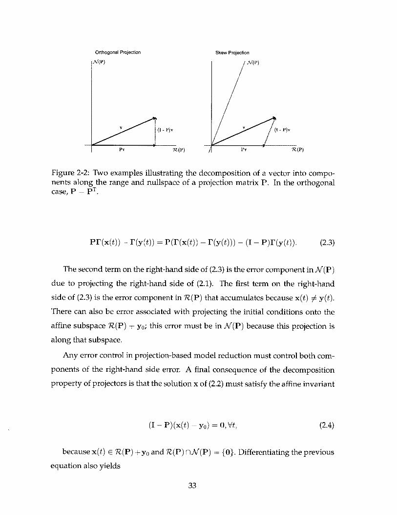
Orthogonal Projection

Ar(P)

(I - P)v

Pv 7 (P) /

Skew Projection

N(P)

V (I - P)v

Pv

Figure 2-2: Two examples illustrating the decomposition of a vector into compo-nents along the range and nullspace of a projection matrix P. In the orthogonalcase, p = pT.

PLF(x(t)) - F(y(t)) = P(Or(x(t)) - IF(y(t))) - (I - P)'(y(t)). (2.3)

The second term on the right-hand side of (2.3) is the error component in M(P)

due to projecting the right-hand side of (2.1). The first term on the right-hand

side of (2.3) is the error component in R(P) that accumulates because x(t) # y(t).

There can also be error associated with projecting the initial conditions onto the

affine subspace R(P) + yo; this error must be in M(P) because this projection is

along that subspace.

Any error control in projection-based model reduction must control both com-

ponents of the right-hand side error. A final consequence of the decomposition

property of projectors is that the solution x of (2.2) must satisfy the affine invariant

(I - P)(x(t) - Yo) = 0, Vt, (2.4)

because x(t) E R(P) +yo and R(P) nM(P) = {O}. Differentiating the previous

equation also yields

33

(I - P)x(t) = 0, Vt. (2.5)

2.3.2 Affine Lumping/Petrov-Galerkin Projection Representation

An equivalent representation may be obtained by lumping state variables [113];

this approach is common in industrial simulations of chemical kinetics. The basic

idea is to replace (2.1) with k similar-looking autonomous "lumped" equations

y(t) = f M)) (2.6)

where y(t) E Rk, and k < n is the number of lumped state variables. A simple

and common method to relate y(t) to an approximation x(t) c Rn of y(t) c Rn is

affine lumping:

y(t) = W T(X(t) - yo), (2.7)

x(t) = Vy(t) + Yo, (2.8)

where V, W E Rnxk are full rank. For the definition of the lumping operation

in (2.7) to be a left inverse of the unlumping operation in (2.8), V and W must

satisfy

WTV = I. (2.9)

In the theory of generalized inverses, the rectangular matrices V and WT are

called {1, 2}-inverses of each other [13]. Note that multiple possible choices of V

and W satisfy both the full rank constraint and the biorthogonality constraint in

(2.9) unless k = n.

34

Differentiating the definition in (2.8) with respect to t and substituting the def-

inition (2.6) in for Y(t) shows that

(2.10)

Defining f: Rk a R k such that

f(~) = f(W T(X(t)- Yo)) = WTf(X(t)) (2.11)

(2.10) becomes

k(t) = VWTf(x(t)) = Pf(x(t)), (2.12)

equivalent to (2.2), where P = VWT is a projection matrix. With this definition

of i, (2.6) becomes

#(t) = W Tf(Vy(t) + yo). (2.13)

One common choice of initial condition for (2.6) and (2.13) is

y(0) = W T (y(0) - yo) (2.14)

under the assumption that x(0) = y(0). However, combining (2.14) with (2.8)

yields the equation

35

:k(t) = VI(y(t)).

x(0) = Vy(O) + Yo = VWT(y(O) - yo) + yo = P(y(O) - Yo) + Yo,

which may or may not satisfy the assumption that x(O) = y(O); this potential

inconsistency illustrates that there is some approximation error in the initial condi-

tion of (2.12), and consequently also in the initial condition of (2.6) and (2.13). One

way to avoid such inconsistency is to set y(O) = yo. However, other choices of yo

may be used for the purposes of accuracy, such as choosing yo so that y(t) decays

onto 'R(P) + yo.

Petrov-Galerkin projection and lumping are identical. Petrov-Galerkin projec-

tion seeks an approximate solution of (2.1) that takes the form

x(t) = yo + Vy(t), (2.16)

where y(t) E R'k, k < n, and V E Rnxk is full rank. Differentiating both sides of

(2.16) with respect to t implies that

k(t) = Vy(t). (2.17)

As is customary in Galerkin-type methods, W E Rnxk is defined so that its

columns are orthogonal to a residual, d(t), defined as

d(t) = *(t) - f(x(t)). (2.18)

Expanding the orthogonality relation

36

(2.15)

WTd(t) = 0

in terms of (2.16) and (2.17) yields

W T [V (t) - f(yo + Vy(t))] = 0. (2.20)

The matrix W is also chosen such that WTV = I (as in (2.9)), so that

y(t) = W Tf(yo + Vy(t)) (2.21)

as in (2.13).

The reason this method is also called a "projection" follows from the observa-

tion that the matrix VWT is a projection matrix; similarly, any projection matrix

P can be decomposed into the product of the form VWT using a full rank de-

composition. This decomposition ensures that V and W have properties consis-

tent with Petrov-Galerkin projection; it can also be shown that R(P) = R(V) and

jV(P) = K(WT) = RI(W)I. Using this decomposition, it can be shown that the

Petrov-Galerkin and projector representations are equivalent: Multiplying both

sides of (2.13) by V and plugging in (2.8) yields (2.2), demonstrating that the two

representations correspond exactly.

A graphical depiction of the affine lumping (Petrov-Galerkin projection) repre-

sentation can be seen in Figure 2-3. In this case, the initial conditions, P, and yo

are the same as those for the reduced system shown in Figure 2-1. The point yo

corresponds to the lowermost point of the dashed and solid curves in the lower

left-hand corner of Figure 2-3; note that the x-axis corresponds to a lumped vari-

able. Temperature is not lumped.

The lumping matrices for Figure 2-3 were obtained by singular value decom-

37

(2.19)

Lumped Representation: Ozone

- - - Original Model- Reduced Model

0.024

0.022-

0.02-

S0.018--0

0.016 -

2 0.014 -

0.012- - - -- . -.. . . 1 .5

0.01- - 2-- - - -2.5

0.008.. ..0.0083 Tirne [s] x 1040.7 0.65 0.6 0.553.50.7 .65 0.6 .55 0.5 0.45 0.4 0.35 0.3 0.25 4

a * Mass Frac 0 + P * Mass Frac 02 + y Mass Frac 03

Figure 2-3: Graphical depiction of Petrov-Galerkin/affine lumping representationfor the same adiabatic 03 decomposition in Figure 2-1. Here, the lumped variableis on the x-axis, and is an affine combination of the mass fractions of 0, 02 and 03;the coefficients of this relationship are the first column of V in (2.23). Note that yois the lowermost point of both curves in the lower left-hand corner; the sharp bendin the upper left-corner indicates that the mass fraction of 0 and lumped variablehave both achieved steady state.

position. Here,

38

6.5428. 10-4

P 1.7751 . 10-2

-1.8405. 10-2

P=VWT= -H

a = 2.5579 - 10-2,

= 6.9397 - 10-1,

-7.1955 - 10-1.

1.7751 . 10-2

4.8159 - 10-1

-4.9935 - 10-1

a / 3 ,

-1.8405. 10-2

-4.9935 .10-1

5.1775 - 10-1

where V and W are as in (2.13). Since V = W for this example, the associated

P is both symmetric and an orthogonal projector.

In Figures 2-1 and 2-3, the initial conditions y* and the value of yo are:

(2.27)(yb, y02, yO3 , T*) = (0, 0.15, 0.85, 1000 K),

(Yo,o, Yo2 ,0, Y03,0, TO) = (9.5669 - 10 3 , 6.8325 - 10-1,

3.0718 - 101, 2.263 - 103 K),

where all calculations are carried out in MATLAB r2012a [133] and Cantera

2.0 [73]; calculations were repeated using Python 2.7.3 [209] and Cantera 2.0 [73].

Details, source code, and input files can be found in Appendix A. In Figure 2-1, the

full model solution is plotted starting from y*, whereas the reduced model solution

is plotted starting from yo. In Figure 2-3, the solutions of both models are plotted

starting from yo.

It is worth noting that both the computational cost and numerical accuracy of

the reduced model solution are dependent on the representation of the reduced

model. Solving (2.13) requires fewer operations than solving (2.2), neglecting the

39

(2.28)

,I(2.22)

(2.23)

(2.24)

(2.25)

(2.26)

influence of matrix multiplies. For NL sufficiently small, each evaluation of both

the right-hand side and the Jacobian of (2.13) requires fewer matrix multiply op-

erations (for V and WT) than the same quantities for (2.2) (for P). For cases of

Petrov-Galerkin projection and projection without special structure, see [165] for

an analysis of computational cost; although POD is considered, results general-

ize to oblique projectors, and focus primarily on matrix multiplies and function

evaluations. Stiffness may also be a factor in comparing the computational costs of

solving (2.13) and (2.2). Generally, (2.13) is no more stiff than (2.2). If (2.13) is much

less stiff than (2.2), it may be possible to use an explicit method to integrate (2.13),

in which case the computational costs of solving (2.13) are much less than solving

(2.2). For examples of this approach using computational singular perturbation,

see [207, 107]. It is important to note that generalizing the conclusions of this para-

graph to the adaptive case is not straightforward. In particular, in the adaptive

case, NL changes with the current system state, changing the sizes of the matrices

V and W, which complicates the preceding discussion considerably, and will be

deferred to future work.

For NL < Ns/2, less memory is required to store the matrix pair (V, W) than

P, and for NL < Ns, less memory is required to store values of the solution y to

(2.13) than is required to store the same number of values of the solution x to (2.2).

Therefore, it is likely that solving (2.13) will require less memory than solving (2.2),

which could be valuable in memory-limited applications, such as in 3-D reacting

flow simulations.

When W consists of standard unit vectors in RNs, computational costs de-

crease, as seen in POD-DEIM [30]. For a fixed P, V and WT are not unique;

replacing them with VQ and Q-1WT, where Q E RNsxNs is invertible, works

equally well from an analytical standpoint, though numerical results may differ.

Good choices of Q can reduce the CPU time needed to solve the reduced model

(2.13) and/or the numerical error in the reduced model solution. Theoretically,

R(P) = R(V) and M(P) = JV(WT) are the important objects, and are unchanged

by such a transformation; they merely yield different diffeomorphisms on the man-

40

ifold 7Z(V) + yo. However, this type of transformation leaves the underlying pro-

jector unchanged, since VQQ-lWT = VWT = P; it cannot convert an orthogonal

projector to an oblique one, or vice versa. Therefore, if the numerical error is neg-

ligible, the same x(t) will be computed for each choice of Q and given t.

However, the numerical error may not be negligible. Given bases for R(P) and

.J(P), calculating P, V, and W accurately in floating point arithmetic is highly

nontrivial; care should be taken to preserve numerical accuracy. See [195] for rec-

ommendations on how to calculate P, V, and W. In order to reduce the numerical

error in calculating the projector-vector product Pv in floating point arithmetic for

any vector v c R", Stewart [195] recommends calculating Pv as VWTv, and set-

ting V and W such that |VH = 1. If |VH WH is greater than |PH, then calculating

Pv in floating point arithmetic using VWTv can lead to a loss in accuracy com-

pared to naively calculating Pv in floating point arithmetic. Stewart also recom-

mends an alternate method for calculating Pv that is at least as accurate because

it does not involve explicitly forming the matrix P. Under certain technical condi-

tions, this alternate method is more accurate than calculating Pv as VWTv; these

technical conditions are rarely satisfied. Furthermore, the numerical error in calcu-

lating Pv using floating point arithmetic increases as IIP I increases, regardless of

calculation method. Since P is singular, condition number is not a useful metric for

numerical error; instead, it is recommended that modelers treat IIP for projection

in the way that they treat the condition number for linear systems, and be alert

for potentially error-prone projection operations. For a thorough analysis of nu-

merical errors associated with calculating oblique projectors and projector-vector

products, see [195].

2.3.3 Affine Invariant/Linear Manifold Representation

As noted earlier, a solution x : R -+ RNs of the reduced model (2.2) satisfies the

overdetermined system

41

k(t) = PL'(x(t)), x(O) = P(y- Yo) + Yo, (2.29a)

0 = (I - P)(x(t) - Yo). (2.29b)

Since I - P is also a projection matrix, a full rank decomposition into I - P =

W1V_ yields a pair of full rank {1, 2}-inverses such that V LW1 = I, Vi, W1 E

RNsx(Ns-NL). The matrices V and W are the same as in the previous section. Using

this information, an equivalent overdetermined system can be formed by premul-

tiplying (2.29b) by VT

k(t) = PF(x(t)), x(O) = P(y- Yo) + yo, (2.30a)

0 VT (X(t) - Yo). (2.30b)

Since VT E R(Ns-NL)xNS is a full rank matrix, there exists a permutation matrix

E E RNsxNs such that VIE can be partitioned into VT E = [L R] such that R E

R(Ns-NL) X (Ns-NL) is invertible, yielding

5(t) = PL'(x(t)), x(O) = P(y* - Yo) + Yo, (2.31a)

0 = [ L R ] E- 1(x(t) - yo). (2.31b)

The entire system can be rewritten by defining

s(t) = E-x(t), (2.32)f(t) J

where s(t) E RNL represents "slow" state variables (e.g., longer-lived, reactive

species compositions) and f(t) E R (Ns-NL) represents algebraically determined

42

state variables (e.g., radical species compositions from linearized steady-state like

approximations, inert species compositions, and species compositions from mass

conservation):

§ (t) = Ir I'L E--IPF (E

f(t) = 0 I(Ns-NL) E 1 PF E

O= [L R s(t)

f (t)

s(O)

f(0)

[[[

s(t)

f(t)

s(t)

f(t)

s(O)

f(0)

,) (2.33a)

(2.33b)

(2.33c)

(2.33d)= E-x(O) = E-l[P(y* - Yo) + yol.

Since the algebraic equation (2.33c) can be solved explicitly for

(2.33b), ignoring (2.33b) yields the affine invariant representation:

f(t) in place of

§(t) =INL 0 E--IPF (E

0 =L R s(t)

f(t) Js(O)

f(O)

[[

s(t)

f(t)

s(O)

f(0)

II,)

= E--x(O).

This representation of the reduced model as a differential-algebraic equation

(DAE) system will be called the affine invariant representation. Since the algebraic

equations are linear and R is invertible, (2.34b) can be solved for f(t) in terms of

s(t):

43

(2.34a)

(2.34b)

(2.34c)

f(t) = f(0) - R-L(s(t) - s(0)). (2.35)

This equation can be substituted into (2.34a) to yield

s(t)(t) = NL [ 1 ] E-PF (E [ f(0) - R-L(s(t) - s(0)) (2.36)

s(0) = INL 0 E0 lx(O),

so the reduced model can also be solved as a systems of NL ODEs; compare

(2.36) with (2.13). This derivation essentially uses the implicit function theorem

[142, 108].

A graphical depiction of the affine invariant representation can be seen in Fig-

ure 2-4. In this case, the initial conditions and yo for the affine invariant system are

the same as those for the reduced system shown in Figure 2-1, but the projection is

chosen such that the mass fraction of 02 is held constant at y0 2 = 6.83252318. 10-1.

This type of approximation (which is obviously inexact, because the sum of species

mass fractions no longer equals one) is commonly used in atmospheric chemistry

when 02 is present in great excess. Consequently, only the mass fractions 0 and

03 are plotted. The point yo corresponds to the intersection of the reduced model

solution and the original model solution in the lower right-hand corner of Figure

2-4; the mass fraction of 02 can be found from this point by subtracting the mass

fractions of 0 and 03 from one. Time increases from right to left.

Reduced models written in this representation, shown in (2.34), are natural if

the modeler knows some conserved or nearly-conserved quantities, e.g., from con-

servation laws or linearized quasi-steady state-like methods. This representation

also gives modelers the option to express their reduced models as DAEs that may

have advantageous structure (such as sparsity, which could make them easier to

solve than (2.2) or (2.13) [183]). However, often, the DAE system is not easy to

44

0.024

0.022 -

0.02-

0.018-Co)

LL 0.016-Ca,

2 0.014-

0.012 -

0.01-

Invariant Representation: Ozone

- - - Original ModelReduced Model

a ... ... .

. . . . . . . . . .

0.008,10 0.05 0.1 015 n 1 r Time[

Mass Frac 03U.0 0.35

s] x 10-

Figure 2-4: Graphical depictions of affine invariant representation for adiabatic 03decomposition; note that this case is different than those in Figures 2-1 and 2-3 inorder to yield a more illustrative plot. Here, the mass fraction of 02 is held constantat yo 2 = 6.83252318 - 101, and the point yo is the intersection of the two curves,found lower right. The sharp bend in the plot corresponds to the establishment of03 = 02 + 0 equilibrium.

solve, and the representation (2.34) is a bit unwieldy due to the number of matri-

ces involved. Typically, the modeler has chosen E, L, R, and yo, which specify

the quantities the modeler wishes to treat as conserved. If one is converting from

one of the other two representations, P is known. Otherwise, if a model reduction

method is originally expressed as a DAE, the modeler will see:

(2.37a)

(2.37b)

If g is affine, if f(t) can be solved in (2.37b) as a function of s(t) for all (s(t), f(t)),

if there exists a permutation matrix E and a projection matrix P such that IF(s(t), f(t)) =

[INL 0]E- 1 PF(E(s(t), f(t)), and if R(P) = {E(s(t), f(t)) : g(s(t), f(t)) = 0} (that is,

45

(t) = f (s(t), f(t)),

0 = g(s(t), f(0)).

4

the algebraic equation defines exactly the range of the projection matrix, after per-

muting the variables so that they have the same order and interpretation as x(t)) all

hold, then (2.37) is an affine invariant representation of a projection-based reduced

model. These four conditions implicitly restrict the values that L and R can take,

via the implicit function theorem. Also, these conditions are not easily satisfied

(or easy to check), and may admit multiple projectors and multiple permutation

matrices. Consequently, it is not easy to determine if (2.37) is an affine invariant

representation. However, an important special case is the linearized quasi-steady

state approximation, which is an affine invariant representation because it can be

expressed in the form of (2.34) with

P = E INL 0 E-1. (2.38)-R-'L 0

For more details on the linearized quasi-steady state approximation, see Section

2.4.3.

2.4 Examples of Projection-Based Model Reduction Meth-

ods

Having established three representations of projection-based model reduction, ex-

amples of methods used in combustion will be presented, categorized by their

classical representation in the literature.

2.4.1 Projector Representation

Two projection-based model reduction methods with classical projector represen-

tations are proper orthogonal decomposition (POD) and the method of invariant

manifolds (MIM).

46

Proper Orthogonal Decomposition

In the ODE context, POD [120, 165] constructs a projected reduced model for (2.1)

by assembling a collection of data points, classically called snapshots, {yi} 'frf such

that yi c RNs for all i. These snapshots are assembled into a matrix

Y =[ (Y1 - Yo) ... (YNref - YO) 1 (2.39)

where yo is usually chosen so that yo = N E ref yi. Snapshots may be data

points from the solution of the original model (2.1), relevant experimental data

points, or other physically realizable points. From this matrix, the SVD (singular

value decomposition; see [200,205]) of Y = UEVT is used to construct the reduced

model. (Here, V is used to distinguish the Hermitian matrix that is part of the

output of SVD from the V matrix of the affine invariant representation.) The rank

NL of the projection matrix is chosen to satisfy an error criterion (see [7] for details).

POD defines a projected reduced model as in (2.2) by P = UNLUT , where UNL

is the submatrix consisting of the first NL columns of U; this result assumes that

the singular values in E are arranged in descending order from left to right, which

is the typical convention for numerical calculations. Note also that for POD, V

W = UNL in (2.8), (2.19), and (2.13), implying that P is an orthogonal projector.

Method of Invariant Manifolds

MIM [74] is motivated by the observation that when (2.1) arises from chemical

kinetics, its solution y : R -+ RNS initially passes through a rapid transient before it

appears to be attracted to a lower-dimensional manifold M c RNs. For sufficiently

large t, the authors of [74] posit that y(t) E M.

MIM uses thermodynamic criteria and an iterative procedure to construct an

NL-dimensional approximation of M called MMI". The remainder of the descrip-

tion of this method requires basic familiarity with smooth manifolds, and is inde-

pendent of the rest of the paper. For any point p E MMIM, there exists a local

47

neighborhood of p, Up c iRNS, a full rank matrix M E RNS xN, a neighborhood of

MTp, VMT c RNL and a smooth (CI) function g : VMTP - Up n MIl such that

MT maps points in Up n4 MMIM to local coordinates on the manifold (in RNL), and g

locally defines the manifold in terms of these local coordinates. The function g and

the matrix M are both defined by MIM [74]. Using these functions, MIM calculates

a projector using the formula

P(w) = Dg(MTw)MT (2.40)

for w C RNs, where Dg is the function defining the Jacobian matrix of g. Since

linear manifolds are assumed, using this formalism requires that the projector

function be evaluated at some point yo E MMIM and treated as a constant, in

which case the projector is evaluated at w = yo. To express MIM in a affine lump-

ing (or Petrov-Galerkin projection) representation, set V = Dg(MTyo) and W = M

in (2.8), (2.19), and (2.13). Nothing restricts P to be an orthogonal projector in this

method; it is typically oblique.

2.4.2 Affine Lumping/Petrov-Galerkin Projection Representation

Three projection-based model reduction methods with classical affine lumping (or

Petrov-Galerkin projection) representations are computational singular perturba-

tion (CSP), linear species lumping (LSL), and reaction invariants (RI).

Computational Singular Perturbation

CSP [103, 104] constructs a reduced model by using a set of vectors called the CSP

basis to determine the range and nullspace of a projection matrix. Let ACSP E

RNSxNs be the CSP basis matrix. It must be invertible, and is calculated from an

initial guess (typically eigenvectors of the Jacobian of F evaluated at a reference

point), followed by optional iterative refinement. Let BCSP (AcsP) 1 be the CSP

reciprocal basis matrix. The number of reduced state variables, NL, is calculated

48

using the error criteria defined by the method. The method also partitions ACSP

and BCSP (again, using the error criteria) in the following way:

AcsP = [CSP ACSP (2.41)f ast slow

FBCSP1BCSP fast (2.42)

slow_

where AcsP c RNsxNL and Bsf E RNLxNs. From these matrices, one con-

structs a reduced model using Petrov-Galerkin projection according to (2.8), (2.19),

and (2.13), with V = ACSP and WT - BcsP. A projector representation follows by

taking P = VWT = AcsPBcSp; this projector is typically oblique. Although AcS'

and Bcs4 are typically matrix-valued functions over RNs, for this analysis, these

functions would be replaced with their values at a reference point yo on the CSP

manifold. In practical applications, the CSP matrices are constructed as piecewise

constant functions over RNS.

Linear Species Lumping

Historically, species lumping has been employed to reduce the computational ef-

fort needed to simulate processes that involve large numbers of species. The gen-

eral idea in linear species lumping [213, 112, 113, 114, 115, 116, 117] is to define

"pseudocomponents" or "lumps" that are linear combinations of species compo-

sitions. These lumps are defined either due to their physical significance (such

as grouping together chemically similar species, or species that react on the same

time scale) or due to their favorable mathematical properties (reducing stiffness,

increasing sparsity).

Linear species lumping uses the mapping y(t) = MLSLy(t) to lump species,

and the map x(t) = MLSLk(t) to unlump species, where MLSL and MLSL are a pair

of full rank (1, 2}-inverses such that MLSL E RNLxNs and MLSL c RNsxNL. It can

be seen by inspection that linear species lumping is a Petrov-Galerkin projection

49

representation as in (2.8), (2.19), and (2.13), where V = MLSL, WT = MLSL, and

yo = 0; as the previous discussion indicates, there is no reason to restrict yo to be

0. Again, P is probably an oblique projector, since it is unlikely that V and W can

be made equal, even with a change of basis.

Reaction Invariants

The method of reaction invariants has been suggested by [211, 64] as a way to re-

duce the computational requirements of simulating chemical reactor systems with

large numbers of species using a change of variables. This change of variables

yields a new set of state variables that can be partitioned into time-varying quan-

tities called variants and time-invariant quantities called invariants. Only the infor-

mation contained in the variants needs to be preserved to reconstruct the solution

of (2.1).

Reaction invariants assumes that (2.1) models chemical kinetics and has the

form I'(y(t)) = Nr(y(t)), where N E RNsxNR is the stoichiometry matrix, r :

RNs y RNR is a function returning a vector of reaction rates, NR is the number

of chemical reactions being modeled, and y : R -+ RNs describes species concen-

trations.

Noting that vectors in AP(NT) correspond to conservation relationships that

hold for this reacting system, let (DRI)T E RNs x (NS-NL) be a matrix whose columns

are a basis for K(NT), where NS - NL = dim(K(NT)). To complete the change of

basis transformation, choose a matrix LRI E RNL xNs such that the change-of-basis

matrix BRI c RNsxNs defined by

BRI [DR1 (2.43)L R1

is invertible. Then the functions v : R -- RNL and w: R -+ RNs-NL such that

v(t) = LRIy(t) and w(t) = DRIy(t) define the variants and invariants of (2.1). Let

50

QRI E RNsx(Ns-NL) and TRI E RNsxNL be matrices such that

(B[RT) = QRI T RI . (2.44)

Setting V = T RI, WT - L RI, and yo = 0 in (2.8), (2.19), and (2.13) illustrates

how the matrices from reaction invariants can be used to carry out model reduction

through Petrov-Galerkin projection. It can also be shown that V1 - (DRI)T, from

which the affine invariant representation

1 (B s(t)

(t) = [ INL 0 E--T LRI F E ,(t) (2.45a)

0 L D1f (t)

R s(t) s(O) s(O)O=D DIE =_f() Lf()LfO E-1y(O), (2.45b)

where

s(t)S(t) Ex(t), (2.46)

and E is an appropriately chosen permutation matrix. It can be shown that

reduced models calculated using reaction invariants are exact, so x(t) = y(t). The

projector P is not necessarily orthogonal, since it is unlikely that V and W can be

set equal in this method, even with a change of basis.

2.4.3 Affine Invariant Representation

A projection-based model reduction method with a classical affine invariant rep-

resentation is the linearized quasi-steady state approximation (LQSSA).

LQSSA was developed by Lu and Law [124] to reduce the computational ex-

51

pense of solving nonlinear equations in the quasi-steady state approximation (QSSA)

by replacing them with (quasi-)linear approximations. Assume in (2.1) that y(t)

can be partitioned such that

yMt) = Ymajor(t), (2.47)L YQSS (t J

where Ymajor(t) E RNL is a collection of known major species and yQSS(t) E

RNS-NL is a collection of known quasi-steady state (QSS) species. The QSSA of

(2.1) is typically expressed as

kmajor(t) = IN 0 Xmajor (2.48a)

LXQSS M )

0 = INS-NL ] Xmajor M (2.48b)XQSS(t)

The initial conditions are discussed at the end of this subsection. LQSSA re-

places the nonlinear algebraic equation in the QSSA DAE (2.48) with a quasilinear

algebraic equation:

Xmajor(t) = INL 0 ] F( Xmaj)or I (2.49a)

(LXQSSM )C~LQSSA r~)(LQSSA D LQSSAxQS)+C, (2.49b)

major Xmajor(t) + (CQSS - )XQSSM + CO)

where CLQSSA c (Ns-NL)xNL LQSSA - DLQSSA c R(NS-NL)x(NS-NL) is in-

vertible, and co c R(Ns-NL). In LQSSA, these quantities are actually functions

defined on RNL (corresponding to the major species), but must be treated as con-

stants here to obtain a linear manifold; these functions are replaced by their values

at Ymajor,O c RNL corresponding to some point yo defined as

52

yo Ymajor,O (2.50)YQSS,O

chosen by the users such that it is a solution to the LQSSA DAE system. (In

practical numerical computations, these matrices are assumed piecewise constant.)

The quantities CLQSSA, CLQSSA - DLQSSA, and co are the coefficients of QSS rela-

tionships linearized (in a manner specific to LQSSA [124], rather than using a Tay-

lor series) at yo. It follows that under these assumptions, the LQSSA DAE system

can be expressed as:

kmajor(t) INL 0 Xmajor (t) , (2.51a)

[ XQSS(t)

0 f-LQSSA ,.LQSSA - DLQSSA Xmajor (t) Xmajor,O (2.51b)0 major QSS D ) XQSS) XQSS,O

which is an affine invariant representation where E = I, L = C , and

R = (CL QSSA - DLQSSA). Since the product P is of the form [IN, 0] E-1 , a projector

representation can be constructed explicitly using (2.38). Let P be the projection

matrix corresponding to this projector representation. If the initial condition of

(2.1) is

y() = y Yajor ' (2.52)tQSS

then the corresponding initial condition for (2.51) is

53

Xmajor (0)x(0) - (0) - P(y* - yo) + yo. (2.53)[XQss(0)J

In this method, P is probably oblique.

2.5 Discussion

Above, it has been shown that many model reduction methods that look super-

ficially very different are all of the same mathematical form given by (2.2). The

accuracy of the reduced models can differ only if they choose different (P, yo). The

numerical efficiency can differ even if P and yo (and thus, reduced model predic-

tions) are identical, depending in part on which of the three formulations of the

reduced model are used. Depending on the choice of the matrix P (or the pair

of matrices V and W), the solution x of the reduced model (2.2) may not satisfy

conservation laws (such as conservation of elements, mass, or energy). However,

it can still give sufficiently accurate results to be useful over time scales of interest.

The major technical obstacle in developing projection-based model reduction

methods is determining a manifold (and a projector P) that gives an accurate re-

duced model. Many researchers in combustion believe that there exist smooth

nonlinear invariant manifolds that can be used to approximate accurately the dy-

namics of stiff ODE systems that arise in chemical kinetics. From a purely theo-

retical perspective, the theory of geometrical singular perturbation theory (GSPT)

[92, 61, 62, 63, 219, 220] and the stable manifold theorem (see Theorem 1.3.2 in

[78]) are cited as reasons that an invariant manifold should exist. However, each

of these results is local in nature; while stable manifolds can be extended using

the flow of an ODE, it is not necessarily clear that the local invariant manifolds of

Fenichel can be extended globally. Furthermore, both GSPT and the stable man-

ifold theorem requires that certain technical conditions be satisfied (see citations

for details). It is not easy to check these conditions in most problems of practi-

54

cal interest. Many systems have some conserved quantities (e.g., number of atoms

in a closed system); these quantities imply exact invariant manifolds. Evidence

suggesting the existence of less obvious invariant manifolds has been observed in

some real-world problems [41,43,40,42,39] as well as simplified model problems

[67, 66, 174, 175, 176, 171, 206, 208]. Therefore, existence of an invariant manifold

is normally assumed, but not proven.

The manifolds used in model reduction in combustion are generally nonlinear

(whether or not they are invariant) due to the significant curvature of trajectories

in applications. Consequently, the linear manifold assumption in projection-based

model reduction is restrictive for problems in chemical kinetics, despite yielding

tractable analysis and useful conclusions; it is very important to remember this

assumption when using these results. In order to be more useful for rigorous com-

putations, the theory needs to be extended to account for piecewise linear or non-

linear manifolds. It is hoped that the streamlined mathematical notation presented

here for linear manifolds will be helpful in that effort.

Although many model reduction methods have the same mathematical form,

very different projection matrices may be used for different purposes. For example,

most of the methods presented are aimed at projecting onto slow modes along fast-

changing modes, but some methods, such as POD and reaction invariants, project

onto fast modes along slow modes.

2.6 Conclusions

In this work, a class of model reduction methods called "projection-based model

reduction methods" was defined, standardizing the language and mathematics

underlying many different methods. It was shown that there are three represen-

tations of projection-based model reduction methods. Sources of instantaneous

approximation error were described. All methods that calculate the same (P, yo)

pair give the same projected reduced model, and thus, under the same initial con-

ditions, the same reduced model solution. From an analytical standpoint the sub-

55

spaces defined by the matrices in the projector and Galerkin representations are

the important objects in determining the accuracy of the reduced model, rather

than the specific matrices themselves. This observation suggests a geometric in-

terpretation of projection-based model reduction. However, clever choices of the

matrices V and W in the affine lumping (or Petrov-Galerkin projection) represen-

tation can reduce the CPU time needed to solve the reduced model, or improve the

numerical accuracy of the reduced model solution. Similarly, clever choices of E,

L, and R in the affine invariant representation could aid in the solution of the DAE

obtained.

Furthermore, it was demonstrated that each of these three representations ap-

pear multiple times in the literature, provided that certain technical assumptions

are made. Where applicable, it was shown how the matrices in each existing

method relate to concepts in projection-based model reduction. The generaliza-

tions about projection-based model reduction methods presented here make it pos-

sible to draw analogies to similar objects in different projection-based model reduc-

tion methods, enabling more systematic comparisons of model reduction methods,

and hopefully spurring more advances in model reduction in combustion.

It would also be useful to develop projection-based model reduction methods

that control error in such a way that it is possible to bound the approximation error

in the reduced model solution relative to the corresponding full model solution.

Observations in this paper, combined with new error bounding results, should aid

in the development of more such methods.

56

Chapter 3

State-Space Error Bounds For

Projection-Based Reduced Model

ODEs

3.1 Introduction

Projection-based model reduction is used in a variety of contexts, including fluid

mechanics [14, 98, 128, 109, 129], control theory [101], atmospheric modeling [59,

48, 193], combustion modeling [103, 104, 124, 188, 206], circuit simulation [20, 169,

170], and other applications to reduce the computational requirements of carrying

out CPU-intensive equation solves. In order to be used with confidence in appli-

cations with stringent accuracy requirements, accurate bounds on or estimates of

the approximation error due to model reduction are needed.

Currently, error bounds for nonlinear ODE systems only exist for the case of

orthogonal projection-based model reduction methods [165] such as proper or-

thogonal decomposition [14] and balanced truncation [8, 6, 7], as well as for the

non-projection-based method POD-DEIM [30, 32, 29]. These error bounds are

based on logarithmic norms of the Jacobian matrix of the ODE right-hand side and

have their theoretical roots in Gronwall's inequality [77] and work by Dahlquist on

57

bounding the error in numerical solutions of ODEs [38]. Although these bounds

typically overestimate the approximation error, in both the numerical ODE con-

text [192, 83, 12] and the context of model reduction of ODEs, they have provided

the basis for work on much more accurate a posteriori estimates of error in both

the numerical solution of ODEs [218, 190, 105] and the approximation error due

to solving reduced model ODEs [86]; again, the estimate in [86] only applies to

orthogonal projection-based model reduction methods.

Similar work on bounding the approximation error due to model reduction

has been carried out by Haasdonk and collaborators [81, 79, 217]. In their work on

model reduction of ODEs, Gronwall- and Dahlquist-like bounds are used to bound

the approximation error in the reduced model solution of linear time-varying pa-

rameterized ODEs for both orthogonal and oblique projection-based model reduc-

tion methods. No effort is made to decompose the error into in-subspace and out-

of-subspace components, as in [165].

Rozza, et al. [178] (and references therein) describe how to construct projection-

based reduced models for affinely parameterized elliptic coercive PDEs with bounds

on the energy norm of the error between a desired functional of the reduced model

solution and the same functional evaluated at a solution obtained using a high-

dimensional finite element approximation. Although the results are presented for

one specific class of PDEs, the authors mention generalizations to affinely param-

eterized linear elliptic noncoercive problems, problems with nonaffine parametric

variation, affine linear (stable) parabolic PDEs, and elliptic (or parabolic) PDEs

with polynomial nonlinearities. However, no rigorous bounds of the same type

exist for elliptic (or parabolic) PDEs with nonpolynomial nonlinearities. Using

these methods, it is also possible to calculate bounds on the residual between

the reduced model PDE solution and the PDE solution obtained using a high-

dimensional finite element approximation [148] (and references therein).

Function norm error bounds on the reduced model solution of Navier-Stokes-

like equations in fluid mechanics in two spatial dimensions were obtained in [102],

assuming POD snapshots in space and backward Euler integration in time; the re-

58

sults require a number of technical inequalities be satisfied, and does not general-

ize easily.

For oblique projection-based model reduction methods, such as DEIM [30],

computational singular perturbation [103, 104], linearized quasi-steady state ap-

proximation [124], and others [156], neither Dahlquist-like bounds nor accurate

long time a posteriori error estimates exist for the approximation error due to solv-

ing reduced model ODEs with nonlinear right-hand sides. Here, the approach of

Rathinam and Petzold [165] is extended from orthogonal projection-based meth-

ods to include all projection-based methods. Although these bounds will not be

tight, as discussed later, they can be used as the basis for future work on a posteriori

error estimation for oblique projection-based model reduction methods.

3.2 Projection-Based Model Reduction

Here, model reduction will be discussed in the ODE setting. Consider the initial

value problem

y(t) = f(y(t)), y(0) =y* (3.1)

where y(t) E R' represents system state variables, y* E R', and f : R- RI

with f E C'.

From (3.1), a projection-based model reduction method constructs a projected

reduced model

x(t) = Pf(x(t)), x(0) = P(y- yo) + yo (3.2)

by calculating a projection matrix P E R7X', where x(t) E R" represents the

state variables of the projected reduced model (which have the same significance

as y(t)), and yo E Rn.

59

An equivalent representation may be obtained through Petrov-Galerkin projec-

tion. In this representation, one seeks a function x : R --+ R approximating the

solution y : R -+ R' of (3.1) that takes the form

x(t) = Yo + Vy(t), (3.3)

where V C R'Xk is a full rank matrix, k < n is the number of reduced state

variables, and y(t) E Rk represents the reduced state variables. The original model

solution and the reduced model solution are related by

y(t) = x(t) - e(t), (3.4)

where the function e : R - R' is the approximation error in the reduced model

solution. Note that e must be differentiable. If x were identically y, then e =

0, because there would be no errors in the reduced model. In practice, e # 0.

Substituting (3.4) into (3.1) and rearranging yields

x(t) - f(x(t) - e(t)) = e(t); (3.5)

typically, in the argument of f in (3.5), the error term is neglected, which will be

the convention in this document. Replacing x(t) in (3.6) with the definition in (3.3),

neglecting the error term in f, and assuming that V is constant yields the definition

of the residual, d(t), of the Petrov-Galerkin projection:

Vy(t) - f(Vy(t) + yo) = d(t). (3.6)

The residual is also defined orthogonal to the range of a full rank matrix W E

Rxk

60

WT(V (t) - f (V(t) + Yo)) = Wd(t) =0, (

subject to the biorthogonality constraint

(3.8)WTV = I.

This constraint, along with equations (3.7) and (3.3), implies that

y(t) = W T (x(t) - yo). (3.9)

Differentiating (3.9) yields the lumped reduced model

y(t) = WTf (V(t) + yo), y(0) = WT(y* - yo). (3.10)

Note that in (3.10), the initial conditions of (3.2) can be used to obtain the proper

initial conditions because P = VWT is the corresponding projection matrix. In the

case where V = W, this process is called Galerkin projection, and the correspond-

ing projector is orthogonal, with P = PT. Otherwise, the corresponding projector

is oblique; the emphasis here will be on the oblique case. For more information

about both of these representations and their equivalence, see [156].

3.3 Mathematical Preliminaries

To bound the state space error in projection-based model reduction, the approach

of this paper will be to bound the norm of a solution to a nonlinear ODE. Following

the presentation of [165], consider the linear system

61

(3.7)

r(t) = Ay(t) + r(t), y(O) = y* (3.11)

for the purpose of illustration, where A E R" xn. The solution of (3.11) takes the

form

y(t) = eAt y* + eA(t-r)r(T) dT. (3.12)

From (3.12), bounds on the norm of y(t) may be derived using Gronwall's

lemma [77] or Dahlquist-like inequalities involving the logarithmic norm of A

[83, 192]. Following the approach of [165], bounds on the norm of the function

y : [0, T] R n7 are derived instead, where T > 0. In this paper, for any function

g: [0, T] -+ R, IIg(t) is the norm of the point g(t) C RTn, assumed to be the 2-norm

unless otherwise stated. The function norm will be denoted I g I and will also be

the 2-norm unless otherwise stated. Keeping function norms in mind, (3.12) may

be written as

y = F(T, A)r + G(T, A)y*,

where F(T, A): L2([0, T],I R) -+ L2 ([0, T], Rn)and G(T, A): Rn -+ L2([0, T], Rn)

are linear operators. The desired bound on y then takes the form

lyll < |jF(T, A)jfl rfl + |HG(T, A)jH yo Hl. (3.13)

Sharp estimates for the operator norms of F(T, A) and G(T, A) are difficult to

obtain. As can be seen from the form of (3.12), these estimates reduce to estimating

the norm of the matrix exponential. The classical approach to this problem [192]

62

yields

lietA < etp(A), t > 0,

where p(A) is the logarithmic norm related to the induced 2-norm of the square

matrix A:

P(A) = rIn + hAll - 1h-+O+ h

The logarithmic norm may be negative, and has the property

max Re Ai < p(A),

where

nonlinear

nonlinear

{Ai} are the eigenvalues of A. Bounding the norm of the solution of a

ODE follows similar reasoning; for a more detailed explanation of the

case, see [83, 192].

3.4 Error Analysis for Projection-Based Model Reduc-

tion

The development of error bounds in this section parallels the presentation in [165].

Consider approximating the solution y : [0, T] -± RI of (3.1) by the solution x :

[0, T] - R' of (3.2) constructed by a projection-based model reduction method. A

bound on the error, e(t) = x(t) - y(t), will be derived. Since R' = 7Z(P) e .V(P),

e(t) maybe decomposed uniquely into e(t) = ec(t)+ei(t), where ei(t) denotes error

within 7Z(P) and ec(t) denotes errors within the complementary subspace fi(P).

Unlike the previous work in [165], ec(t) and ei(t) are not necessarily orthogonal

63

because P may be an oblique projector. These errors can be expressed as

ec(t) = (I - P)(x(t) - y(t)) = -(I - P)y(t) + (I - P)yo (3.14)

ei(t) = P(x(t) - y(t)). (3.15)

The component ec(t) is the error between y(t) and its projection onto R(P)

along K(P). It is assumed that P is calculated by a projection-based model reduc-

tion method that bounds ec(t) in some norm to within a specified tolerance; this

assumption will be revisited after error bounds are derived.

Typically, e (t) is not explicitly bounded by a method; it consists of errors in

R(P) that accumulate over time as ec(t) increases in norm.

An error estimate for ei(t) can be derived in terms of ec(t). Differentiating (3.15)

and substituting (3.1) and (3.2) for the resulting time derivatives and initial condi-

tions yields

ei(t)=P[f(y(t) + ec(t) + ei(t)) - f(y(t))], e(O) =0. (3.16)

Note that ei(O) = 0 because the initial conditions of (3.1) are projected onto

R(P) along M(P) in (3.2). Therefore, ei(t) is governed by (3.16), where ec(t) and

y(t) may be treated as forcing terms. For a graphical illustration of the relation-

ships among y, x, ec, ei, and e, see Figure 3-1.

Before presenting error bounding results for the nonlinear ODE case, it is in-

structive to consider error bounding results for the linear case. Suppose that (3.1)

takes the form y(t) = Ay(t) with A E Rnx . Then (3.16) becomes

6i(t) = PAe2 (t) + PAec(t), ei(0) = 0.

It will be useful to define V 1 and W 1 as matrices whose columns span R7(V)'

64

Y

e(t)

y (O) eC (t

e (t)e (0 ) ..-. .. ....._.....x

x(0) = y(0)

R (P) + YO

Figure 3-1: Illustrates the relationships among the full model solution y, the pro-jected solution ' (see (3.22)), the reduced model solution x, and the error e. Notethat the error is decomposed into a component in R(P) denoted ei, and a compo-nent in K(P) denoted e.

and R(W)', respectively, that also satisfy the relationship

VT W 1 = I. (3.17)

These matrices will be used in developing error bounds for reduced order mod-

els. It follows that V1 , Wi E Rnx(n-k); these matrices also satisfy I - P = W I ,

and can be obtained via full rank decomposition of I - P. This decomposition is

not unique.

For convenience, let A = WTAV c R kxk, and A = WTAW1 c Rk x(n-k). Then,

using the result in (3.13) and a change of coordinates yields the bound

ileil <; ||F(T, A-)||||AI|||VI|||V-L|||lecll,

65

so the total error is bounded by

|lell < (JIF(T, Ai) 11JJA 1 ||IV II I|V -11+ 1) Ilecl.

Here, A = WTAV E Rkxk, and = WT AWI e Rkx(n-k), where V 1 and W 1

are matrices whose columns span 7Z(V)' and R(W)', scaled so that VTWi = I.

Then V 1 , Wr E Rnx(,-k); these matrices also satisfy I - P = WIVT, and can be

obtained via full rank decomposition of I - P.

The nonlinear case proceeds in a similar fashion. Write the solution y: [0, T] -

R" of (3.1) and the solution x : [0, T] -+ R of (3.2) as

y(t) = Vu(t) + Wiv(t) + yo, (3.18)

x(t) = Vu(t) + Vw(t) + yo = y(t) + e(t), (3.19)

so that the errors ec(t) and ei(t) and the projected solution y [0, T] - R' are

given by

ec(t) = -Wiv(t) = y(t) - y(t), (3.20)

ei(t) = Vw(t) = x(t) - y(t), (3.21)

'(t) = y(t) + ec(t) = Vu(t) + yo = P(y(t) - yo) + yo. (3.22)

Note that u(t) E Rk, w(t) E Rk, v(t) E Rn-k, and k = tr(P). Recalling that

P = VWT is a full rank decomposition of a projection matrix P such that WTV - I,

the linear case can be generalized in the following theorem:

Theorem 3.4.1. Consider solving the initial value problem (3.1) using the projection-

based reduced order model (3.2) in the interval [0, T]. Let -y > 0 be the Lipschitz constant

of WTf in the directions corresponding to MA(P) = AF(WT) = 7Z(W)' in a region con-

66

taining y([O, T]) and '([0, T]). To be precise, suppose

IWTf (y(t) + Wv) - W Tf( (t)) < 'YIVI

for all (v, t) E A c Rn-k x [0, T], where the region A is such that the associated region

A = {(y(t) + Wiv, t) : (v, t) E A} contains (y(t), t) and (y(t), t)for all t in [0, T]. Let

p(WTDf(yo + Vz)V) < pfor z E V C Rk, where {u(t)+ Aw(t) : t c [0, T], A E [0, 1]}

is contained in V, and p(.) denotes the logarithmic norm related to the 2-norm.

The function ej satisfies

inf{C > 0: |jej(t)||o < Ca.e. on [0,T] } = |jeiIK, < { vj2 _ 1/2||VK|||VTl1,

E, T1/2||V||||Vill,

and the 2-norm of thefunction e satisfies

Ie(t) 112 dt 1/2= | | e l <

E( 1+ 7.)je2ftT-2pT)/ 2 |VIIvII VII,4[Z2 -L)

E(1 + 2-1/2yT1VII |VI V ),

where

rT 1/2

|11e.11 = ( I ec(t)112 dt (3.25)

Proof. The proof follows the development of Proposition 4.2 in [165]. Since ei(t) =

Vw(t) and WTV = Ik, it follows that WTei(t) = w(t), so

67

f f 0,

f = 0,

(3.23)

f f 0,

f =0,

(3.24)

*(t) = WTeI(t) = WTf(y(t)) - WTf(x(t)),

and

*(t) = WTf(yO + Vu(t) + Vw(t)) - WTf(yo + Vu(t) + Wv(t)). (3.27)

Applying a Taylor expansion for h > 0, w(t + h) = w(t) + h-&(t) + 0(h2 ), which

satisfies

11w(t + h)HI = ||w(t) + h*(t) + O(h 2)11

= 11w(t) + hWTf(yo + Vu(t) + Vw(t)) - hWTf(yo + Vu(t) + Wv(t)) + O(h 2)11.

(3.28)

Using the triangle inequality on the previous equation (3.28) yields

I1w(t + h)|1 < 1w(t) + hWTf(yo + Vu(t) + Vw(t)) - hWTf(yo + Vu(t))H

+ h lWTf(yo + Vu(t) + Wv(t)) - WTf(yo + Vu(t)) 11+ O(h 2).

(3.29)

Let g : R' -+ Rk be the function

g(?I) = 7) + hWTf(yO + V71). (3.30)

Then

68

(3.26)

||w(t) + hW Tf(yo + Vu(t) + Vw(t)) - hW Tf(yo + Vu(t)) = |1g(u(t) + w(t)) - g(u(t)) .

(3.31)

Applying a multivariate mean value theorem (Exercise 2.5 from [52]) to g yields

||g(u(t) + w(t)) - g(u(t))1 < ,'1w(t)H1, (3.32)

for any K E R such that

K > supvjc[u(t),u(t)+w(t)

||Dg(n)fl supne[u(t),u(t)+w(t)]

1Ik + hWTDf(yo + Vq)VII.

Here, for any two vectors 1, m2 E Rk, [77, 2] denotes the line segment join-

ing the two. (Traditionally, this bracket notation refers to intervals; however, the

convention used by Rathinam and Petzold [165] is followed here.) Since the line

[u(t), u(t) + w(t)] is a compact subset of Rk,

1Ik + hWTDf(yo + V?)V 1 = max'1E[U(t),U(t)+w(t)]

|1Ik + hWTDf(yo + Vq)V 1.

It follows from (3.31), (3.32), (3.33), and (3.29) that

1w(t + h)H1 - ||w(t)| 1 max?7G[u(t),u(t)+w(t)]

1|Ik + hWTDf(yo + Vq)VII - 1 ||w(t)J|

+ h IWTf(yO + Vu(t) + WJv(t)) - WTf(yO + Vu(t)) 1 + O(h 2),

< max lIk + hWTDf(yo + Vq)V+E[Uyl,U(It)+W(t))

+ h- Jlv(t)|| + O(h 2),

- ~1w(t)1

(3.34)

69

(3.33)

sup'qE[U(t),U(t)+w(t)]

which implies that

|1w(t + h)1 - ||w(t)l 1 pllw(t)| 11+ 'yllv(t)|1 + O(h),h

(3.35)

where the O(h) term may be uniformly bounded independent of w(t) (see [83],

Equations 10.17 and 10.18). Then it follows from Theorem 10.6 of [83] that

(3.36)

Since ej(t) = Vw(t), it follows that

||ej(t)jj < |VH flw(t)II < V I efA(tr) IIv(T) dr. (3.37)

After applying the Cauchy-Schwarz inequality on the right-hand side, it fol-

lows that

i|ei(t)II <ll ('iv(T)H 2

IVIlti/2 ( f t|v(r) 12 dT /

Since v(t)= -VTI e(t), it follows that

lei(t)HI <| I V I I I I V T 1 1 7 2e c/) 1 /2 d ,

Iv V | (/2p ( 2f ecr) 2 dT

JIV II JVT 11_YI/2 e,( )12 -1/2

from which it follows that

70

(3.38)P = 0.

p # 0,

p = 0,(3.39)

||wWt)| < - J eft)II v(-r) I dr.

dT)

||eill < {at7-1 1/ ||VI|V fI t p 0,

E&T 112 |VfIVI, ft = 0.(3.40)

Substituting (3.25) then squaring (3.39), integrating, and taking the square root

to pass to the L2 -norm yields the bound

leiHl <(e2T-1-2rT 1/2

2- 1/ 2EyTVH VI IVII,

f # 0,

ft=0.(3.41)

Applying the triangle inequality yields

Iell < Ieill + Iec1| <{ (e2T1-2pT)E 1 +

E(1 + 2- 1/ 2yTII VII |VII),

Remark 3.4.2. When p < 0, uniform bounds (independent of T) can obtained from

Theorem 3.4.1 by noting that

e2 tt _1 1-,

P |p|(3.43)

in which case

||ell < E (1

(3.44)

(3.45)+ |L ).

Remark 3.4.3. It is worth noting that if Theorem 3.4.1 is applied to an orthogo-

71

p # 0,

t=0.

(3.42)

El

1/2||IV II |V Tl 1

||ejIjll < E712 il -1/2||IV I||I IIT1,

nal projector, the resulting bounds are weaker than those derived in [165] because

orthogonality is not used in the proof above. Also note that the since full rank de-

compositions of P and I - P are not unique, the error bounds derived in Theorem

3.4.1 are not unique, and depend on these full rank decompositions. Some choice

of these decompositions will yield the tightest possible error bounds. However,

worst-case error bounds may be derived by changing the approach above slightly.

Write instead the solution x : [0, T] -+ Rn of (3.2) in terms of the solution y

[0, T] -+ R n of (3. 1):

x(t) = y(t) + ec(t) + ei(t).

Write the projected solution y: [0, T] -+ R" as

y (t) = y(t) + ec(t).

Then error bounds can be obtained from the following corollary:

Corollary 3.4.4. Assume the hypotheses of Theorem 3.4.1. Let Y' > 0 be the Lipschitz

constant of Pf in the directions corresponding to M(P) in a region containing y([O, T])

and y([0, T]). To be precise, suppose

|lPf(y(t) + Wv) - Pf(y(t)) < '/Hv

for all (v, t) c A' c Rn-k x [0, T], where the region A' is such that the associated region

A' = {(y(t) + Wv, t) : (v, t) c A'} contains (y(t), t) and (y(t), t) for all t in [0, T], and

W1 is orthonormal.. Let p(PDf(z)) < p'for z E V' C Rn, {Ay(t) + (1 - A)x(t) : t E

[0, T ], A c [0, 1]} is contained in V', and bt(-) denotes the logarithmic norm related to the

2-norm.

The function ei satisfies

72

I( ______ -1 1/2

inf{C > 0 : lei(t)| I C a.e. on [0, T] } = |leiH00 < e2A1 _, 1 0

S T/,t 1 0,

(3.46)


T 1/2 fe ( ,/'e - 1-2pT' 1/2

Ile(t) 12 dt = Ilell < (3.47)

e(1 + 2-1/2 y'T), ' 0.

Proof. Only a sketch proof will be provided; the proof follows the logic of Theorem

3.4.1, but uses the decomposition

I|ei(t + h) 1 = 11ei(t) + hPf(y(t) + ec(t) + ei(t)) - hPf(y(t)) II+ 0(h2 )

< |lei(t) + hPf(y(t) + ec(t) + ei(t)) - hPf(y(t) + e,)

+ hflPf(y(t)) - hPf(y(t) + e,) 1 + 0(h2 ) (3.48)

instead of (3.29) to derive bounds. E

Remark 3.4.5. The bounds in Corollary 3.4.4 do not correspond to the bounds in

Theorem 3.4.1, because ft and ft' cannot be compared directly, since they bound the

logarithmic norm of square matrices of differing size. Coordinate changes cannot

be used to relate the logarithmic norm in the hypotheses of Theorem 3.4.1 to the

logarithmic norm in the hypotheses of Corollary 3.4.4; these coordinate changes

would not be norm-preserving. Bounds corresponding to Corollary 3.4.4 were not

considered in [165]; the likely explanation for not considering this approach in

that work is that IIP = 1 for the case where P is an orthogonal projector, and V,

W, V 1 , and W 1 can all be chosen such that their 2-norms are all one. Corollary

73

3.4.4 yields worst-case bounds on the error for a projection-based model reduc-

tion method, since these bounds are unique, unlike the bounds in Theorem 3.4.1.

However, these bounds are generally expected to be weaker than Theorem 3.4.1,

because the hypotheses involve taking the logarithmic norm of a larger square

matrix, making it more likely in practice to yield a large logarithmic norm bound,

compared to Theorem 3.4.1.

Remark 3.4.6. By considering in-subspace errors (ei(t), which is in R(P)) and out-

of-subspace errors (ec(t), which is in X(P)) separately, this analysis provides a

bound on the norm of the total error function, e, in terms of 6, a bound on the

norm of the out-of-subspace error function, e. The value of E depends on the

solution y : [0, T] - R n of (3.1) and on P and yo in (3.2). In general, IIeH is not

known precisely unless the solution of (3.1) is calculated; this observation holds

even for the analysis of POD in [165]. Typically, a bound on IIe, | is estimated using

any error control results provided by a model reduction method. If such results are

unavailable, substituting a known solution to (3.1) with different initial conditions

that approximates y is another way to obtain such an estimate. Using an estimate

of e in Theorem 3.4.1 or Corollary 3.4.4 would only yield estimates of bounds on

the function norm of the total error at best; if the function used in place of y in the

definition of (3.14) differs significantly from y, these estimates may be inaccurate.

Consequently, such estimates must be used with caution.

3.5 Case Study

To illustrate the factors affecting bounds on the norms of ei and e given e, (or

bounds on IIe, 12), consider the linear time invariant ODE

y(t) = Ay(t), y(0) = y (3.49)

where A takes the form

74

A= A1 A 1 2 1 (3.50)0 A2

with the blocks of A first taking the values

-2.1 0 0

A= 0 -2.1732 -2 (3.51)

0 -2 -2.1732

0.3893 0.5179 -1.543

A12 1.39 1.3 0.8841 (3.52)

0.06293 -0.9078 -1.184

-3 0 0

A 2 0 -3.226 -0.708 , (3.53)

0 -0.708 -3.226

so that n = 6. Three values of A were considered; modifications of (3.51), (3.52),

and (3.53) will be discussed later in this section. This example is inspired by [165];

the matrix A in this paper differs from the matrix A in that paper by negating

all positive entries of A1 and A 2 in [165], then subtracting 21 from the resulting

matrix. These manipulations can be seen in the accompanying MATLAB [133] and

Python [209] code in Appendix B.

Unlike the case of orthogonal projectors, it is impossible to use a norm-preserving

change of basis to decouple the effects of E, -y, and p, because R(P) is not orthog-

onal to M(P) when P is an oblique projector. Consequently, when changing one

of {E, 7y, f}, at least one other parameter changes. In light of this observation, the

effect of changing y and E at constant p, and the effect of changing p and F at

constant -y were studied by altering the blocks of A. The parameters 'y and ft were

calculated using -y = |WT AW 1|2 and p = p(WTAV); both formulates derive from

75

Theorem 3.4.1. The parameters y' and p' were calculated using -y' = IPAW 1|2 and

' = p(PA), where W1. is orthonormal. The parameter e and all other function 2-

norms were calculated by approximating definite integrals using the trapezoidal

rule.

Note that A 1 and A 2 in (3.51) and (3.53), respectively, are symmetric and have

negative real eigenvalues. Furthermore, the spectrum of A is the union of the

spectra of A 1 and A 2. For each value of A considered, the projector P is chosen so

that R(P) consists of the three eigenvectors of A that are not contained in the span

of {ei, e 2 , e3 }, where ej is the jth standard Euclidean unit vector; consequently,

the number of reduced variables is k = 3. However, for all three values of A

considered, K(P) will always be spanned by {e 4 , e5 , e6}, where again, ej is the jth

standard Euclidean unit vector. As a result, when A changes, the projector P will

change with it, because the range of the projector changes, even though the null

space of the projector will stay the same.

To illustrate the effect of changing V, W, V 1 , and W 1 on the error bounds

given by Theorem 3.4.1, two sets of values for these matrices will be considered. In

the first set of values, W and W 1 will have orthonormal columns so that ||WI12 =

||W-||2 = 1; the remaining matrices are determined so that they satisfy (3.8) and

(3.17). In the second set of values, V and V 1 have orthonormal columns so that

|JV1| 2 = ||VI112 = 1; the remaining matrices are determined so that they satisfy

(3.8) and (3.17). The error bounds obtained from Theorem 3.4.1 were compared to

error bounds obtained from Corollary 3.4.4.

The matrices V, W, V 1 , and W 1 were calculated from matrices whose columns

spanned R(P) and M(P), respectively, using the algorithm suggested in equations

(5.1) and (5.2) of [195]. Projector-vector products were also calculated using this

algorithm. While explicit calculation of P is not recommended [195], it was cal-

culated explicitly only to calculate I|P1l2 to get an idea of numerical errors due

to projector-vector products. The quantity I|PI12 plays a role in the calculation

of projector-vector products similar to that of the condition number when solv-

ing systems of linear equations [195]. All ODEs were integrated using an explicit

76

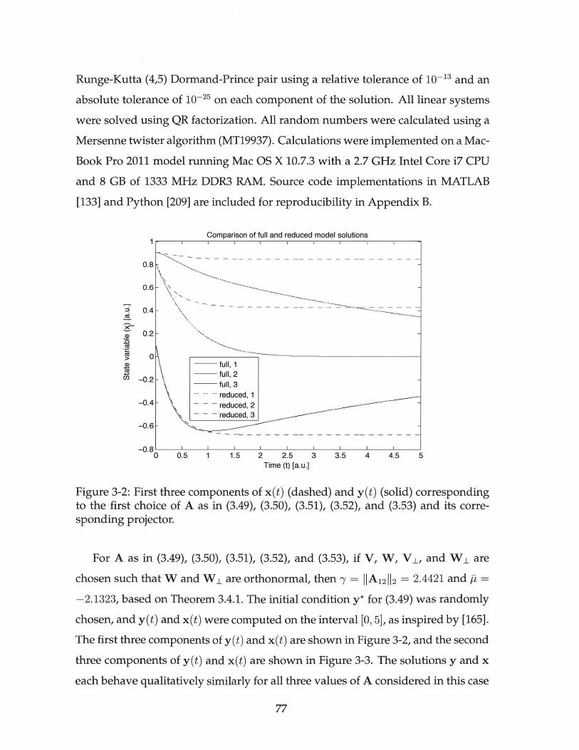
Runge-Kutta (4,5) Dormand-Prince pair using a relative tolerance of 10-13 and an

absolute tolerance of 10-25 on each component of the solution. All linear systems

were solved using QR factorization. All random numbers were calculated using a

Mersenne twister algorithm (MT19937). Calculations were implemented on a Mac-

Book Pro 2011 model running Mac OS X 10.7.3 with a 2.7 GHz Intel Core i7 CPU

and 8 GB of 1333 MHz DDR3 RAM. Source code implementations in MATLAB

[133] and Python [209] are included for reproducibility in Appendix B.

Comparison of full and reduced model solutions

0.8 -

0.6 -

0.4 \ ~-~~

x 0.2-Ca

0- - full, 1

- . -full, 2Cn -0.2 full, 3

-0.4- - - - reduced, 2- - - reduced, 3

-0.6 --

00 0.5 1 1.5 2 2.5 3 3.5 4 4.5 5Time (t) [a.u.]

Figure 3-2: First three components of x(t) (dashed) and y(t) (solid) correspondingto the first choice of A as in (3.49), (3.50), (3.51), (3.52), and (3.53) and its corre-sponding projector.

For A as in (3.49), (3.50), (3.51), (3.52), and (3.53), if V, W, V 1 , and W 1 are

chosen such that W and W 1 are orthonormal, then -y = IIA 12 112 = 2.4421 and P =

-2.1323, based on Theorem 3.4.1. The initial condition y* for (3.49) was randomly

chosen, and y(t) and x(t) were computed on the interval [0, 5], as inspired by [165].

The first three components of y(t) and x(t) are shown in Figure 3-2, and the second

three components of y(t) and x(t) are shown in Figure 3-3. The solutions y and x

each behave qualitatively similarly for all three values of A considered in this case

77


0.8 full, 4full, 5full, 6

0.6 - - -reduced, 4- - - reduced, 5- - - reduced, 6

0.4-

CO

0.2-

0 -

-0.2 -

0 0.5 1 1.5 2 2.5 3 3.5 4 4.5 5Time (t) [a.u.]

Figure 3-3: Second three components of x(t) (dashed) and y(t) (solid) correspond-ing to the first choice of A as in (3.49), (3.50), (3.51), (3.52), and (3.53) and its corre-sponding projector.

study, and will not be plotted for other values of A. The first three components

of ei(t) and e(t) are shown in Figure 3-4; note that ej (t) = ei(t) for j = 1, 2, 3 and

all t on [0, 5]. The second three components of ei(t) and e(t) are shown in Figure

3-5. As with y(t) and x(t), the quantities ei(t) and e(t) each behave qualitatively

similarly for all three values of A considered; no additional plots of ei(t) or e(t) will

be presented. The 2-norm of the component of the error in K(P) was e = IIe,112 =

2.3423. The sup-norm and 2-norm of the component of the error in R(P) were

|Hei 11,,= 1.1659 and Heill2 = 2.3950. The 2-norm of the total error was IIe112 = 1.7180.

The bounds provided by Theorem 3.4.1 when W and W 1 are orthonormal are

I|ei|Io < 1.9937-101, fleil12 5 4.3524-10 1, and |1e||2 <4.5866.101. When V and Vi are

orthonormal, -y = 1.0727.101 and ft = -2.4588, illustrating that choice of V, W, V 1 ,

and W 1 does affect the error bound provided by Theorem 3.4.1. Using Corollary

3.4.4, y' = 6.1365 and A' = 3.0048; the positive value of p' indicates that the error

bounds provided by Corollary 3.4.4 would be much worse than the error bounds

78

1

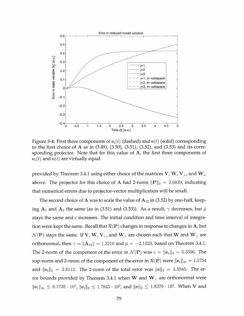
Error in reduced model solution0.6

0.5-

0.4-

0.3-

A 0.2- =2j=3

0.1 - - - j=1, in-subspace-- - j=2, in-subspace

a) --- j=3, in-subspace

-0.1 -

-0.2-

-0.3-

00 0.5 1 1.5 2 2.5 3 3.5 4 4.5 5Time (t) [a.u.]

Figure 3-4: First three components of ei(t) (dashed) and e(t) (solid) correspondingto the first choice of A as in (3.49), (3.50), (3.51), (3.52), and (3.53) and its corre-sponding projector. Note that for this value of A, the first three components ofei(t) and e(t) are virtually equal.

provided by Theorem 3.4.1 using either choice of the matrices V, W, VI, and W 1

above. The projector for this choice of A had 2-norm IIP112 = 2.6829, indicating

that numerical errors due to projector-vector multiplication will be small.

The second choice of A was to scale the value of A 12 in (3.52) by one-half, keep-

ing A 1 and A 2 the same (as in (3.51) and (3.53)). As a result, -y decreases, but P

stays the same and 6 increases. The initial condition and time interval of integra-

tion were kept the same. Recall that 7Z(P) changes in response to changes in A, but

JV(P) stays the same. If V, W, V 1 , and W 1 are chosen such that W and W 1 are

orthonormal, then -' = IIA121I = 1.2210 and p = -2.1323, based on Theorem 3.4.1.

The 2-norm of the component of the error in K(P) was e = IIe,112 = 5.3596. The

sup-norm and 2-nrom of the component of the error in 7Z(P) were Iei Ij' = 1.5754

and IeiI12 = 2.8112. The 2-norm of the total error was |He|I2 = 3.5945. The er-

ror bounds provided by Theorem 3.4.1 when W and W 1 are orthonormal were

I|eillo, < 8.1735- 101, |lei||2 < 1.7843 - 102, and jell12 < 1.8379. 102. When V and

79

0.6

0.4

0.2

0

-0.2

-0.4

-0.6

-0.8

-1

1 2

Error in reduced model solution

0 0.5 1 1.5 2 2.5Time (t) [a.u.]

3 3.5 4 4.5 5

Figure 3-5: Second three components of ei(t) (dashed) and e(t)ing to the first choice of A as in (3.49), (3.50), (3.51), (3.52), andsponding projector.

(solid) correspond-(3.53) and its corre-

V 1 are orthonormal, -y = 1.7260 - 101 and P = -2.5041, according to Theorem

3.4.1. Using Corollary 3.4.4, -y' = 5.7798 and p' = 5.8023. This projector for this

choice of A had 2-norm IIP112.= 5.0786, indicating again that numerical errors due

to projector-vector multiplication will be small.

The third and final choice of A was to keep A, and A 12 as in (3.51) and (3.52),

and scale the value of A 2 in (3.53) by .715, so that y stays the same and both P and

e increase, relative to the first choice of A. If V, W, V 1 , and W 1 are chosen such

that W and W± are orthonormal, then -y = IIA 12 112 = 2.4421 and p = 4.8194. 10-1,

based on Theorem 3.4.1. The 2-norm of the component of the error in fi(P) was

E = |IeCH|2 = 3.4998. The sup-norm and 2-norm of the component of the error in

R(P) were |1eill.. = 1.6444 and |1eil12 = 3.7803; the 2-norm of the total error is

|e||2 = 5.5926. The error bounds provided by Theorem 3.4.1 when W and W 1 are

orthonormal are I Iei<11,, 9.9526 - 102, |ei1l12 < 9.9366 - 102, and le||2 < 9.9716 - 102.

According to Theorem 3.4.1, when V and V 1 are orthonormal, -y = 9.3634 and ft =

80

cd

CO

cn

N -~N

NN

NN

N

j=4j=5j=6

- - - j=4, in-subspace- - - j=5, in-subspace- -- j=6, in-subspace

I I I I

- .

I

-1.2220. Using Corollary 3.4.4, -y' = 5.0389 and p = 5.9639; here, IIP 12 = 3.2114.

3.6 Discussion

From the error results in Theorem 3.4.1 and Corollary 3.4.4, inferences can be made

about how choices of P, V, W, VI, and W 1 affect the error bounds, as well as the

error, to a first approximation. Discussion will focus on Theorem 3.4.1, though

similar observations also apply to Corollary 3.4.4.

The three primary factors influencing bounds on the error due to model re-

duction are the parameters c, -y, and p. As noted earlier, E is controlled by a model

reduction method in the ideal case; if the reduced model is chosen well, using tight

error tolerances, E will be small.

To interpret y and p, it will be useful to introduce some additional mathematical

background. Let q : S c X -± X be a nonlinear map, where X C R"n. The least

upper bound (lub) Lipschitz constant of q, L(q), is defined in [192] as

L(q) = sup .-(3.54)u,veS,usv fu - vfl

It has the property that

|jq(u) - q(v) 1 < L(q) - |ju - v1, Vu, v E S, (3.55)

and if S is convex and q is differentiable, then

L(q) = sup ||Dq(u)jj. (3.56)uES

In the hypotheses of Theorem 3.4.1, define the function g : Rn-k x RI -* R k by

81

g(v, z) = WTf(z + Wiv). (3.57)

If the set A is convex, then the best value of the Lipschitz constant -y is sup{L(g(-, z))

Z E y([0, T])}1.

The extension of the logarithmic norm to nonlinear maps will also be useful for

discussion. The least upper bound logarithmic Lipschitz constant of q, M(q), is

defined in [192] by

(3.58)M(q)= lim L(I + hDq) - 1h-+0*+ h

The lub logarithmic Lipschitz constant generalizes the logarithmic norm; for

a square matrix A, M(A) = p(A). Furthermore, if q is differentiable, and S is

convex,

M(q) = sup pt(Dq(u)).uES

(3.59)

In the hypotheses of Theorem 3.4.1, if the set V is convex, then the best value of

the bound p on the logarithmic norm is M(h), where h : Rk + Rk is defined by

h(y) = W Tf(yo + Vy). (3.60)

The concepts of lub Lipschitz constant and lub logarithmic Lipschitz constant

can be used to a prove a result like Theorem 3.4.1; such an approach was taken

in [29] to prove error bounds on POD-DEIM reduced models, and would yield

bounds that are essentially the same as those in Theorem 3.4.1. Their utility here is

in interpreting the meaning of the bounds stated in Theorem 3.4.1.

82

Let e'h : f(0) - g(t) be the flow corresponding to the differential equation

y(t) = h(y(t)) = W Tf(yo + Vf(t)), (3.61)

as in (3.10). Then it can be shown [192] that

L(eth) < e tM(h) < etA. (3.62)

In other words, p corresponds to the maximum rate of change of the solution

to (3.10) and (3.61). In the ideal case, if a reduced model is chosen well, k (i.e.,

the rank of the projection matrix, or the number of variables in a Petrov-Galerkin

representation of a reduced model [156]) will be small, and the solution y : [0, T] -+

Rk will change slowly with time, enabling cheap numerical integration of (3.10).

Consequently, in the ideal case, p will be small.

The constant -y > sup{L(g(-, v)) : v E ([0, T])} corresponds to the maximum

rate of change of the right-hand side of the lumped system (3.10) in the directions

corresponding to M(P) = R(W)' = R(W1 ). In other words, it is the maximum

rate of change of the right-hand side of (3.10) in directions neglected by the reduced

model. When (3.1) is a stiff system, certain directions in state space are associated

(locally, in the case of nonlinear systems) with fast rates of change in the solution

y : [0, T] -- R and also fast rates of change in the time derivative of y. These direc-

tions associated with fast changes are usually candidates for inclusion in fi(P) so

that solution of the resulting lumped system changes slowly; rapid transients are

usually neglected. Consequently, in stiff systems, if p is small because a good re-

duced model is chosen by cleverly choosing V and W, - is likely to be large. One

would expect some tradeoff between p and - in stiff systems, depending on the

choice of reduced model (i.e., choice of V and W); if directions corresponding to

fast changes are included in R(P), ft is likely to be large, and 7 is likely to decrease.

As a result, the bounds in Theorem 3.4.1 are expected to overestimate the error, es-

83

pecially for large values of T; in all likelihood, for stiff systems, they will drastically

overestimate the error due to model reduction, but do provide some insight into

factors affecting error. For researchers designing reduced models, the key insight

is to choose V and W to minimize p; y is a secondary consideration. Both the

overestimation of error and insight into factors affecting error are in keeping with

the use of the logarithmic norm to bound the error due to numerical integration of

ODEs; the logarithmic norm yields very large bounds for stiff systems, but these

bounds are in terms of the step size h. Typically, h can be chosen sufficiently small

so that stability and error criteria are satisfied, yielding useful bounds for short

times only.

The remaining parameters in the error bounds in Theorem 3.4.1 have less in-

fluence on the error bounds. There is some freedom in choosing the end time,

depending on the needs of the user, but the exponential dependence of the bounds

on time suggests that the result will over estimate the error for long times if p > 0,

which includes many applications of interest. (It is worth noting that P > 0 does

not imply that an ODE is unstable, unless the right-hand side of an ODE has a

symmetric Jacobian matrix. (Linear) Stability of an ODE system is dictated by the

eigenvalues of the Jacobian matrix of its right-hand side.) Since full rank decom-

positions of projection matrices are not unique, there is freedom in choosing V and

VI; for numerical calculations with the Petrov-Galerkin (lumped) representation,

the product IIVIIIIWII should be as close to IIPII as possible [195]. For a thorough

discussion of the numerical analysis associated with calculating oblique projection

matrices, as well as oblique projector-vector products, consult [195]. Note that

||PJ| = 1 if and only if P is an orthogonal projector. If P is an oblique projector,

P > 1. Choices of V, V 1 , W, and Wi will also affect -y and p indirectly.

3.7 Conclusions and Future Work

In this work, state space error bounds for projection-based model reduction meth-

ods were derived in the nonlinear ODE setting in terms of the function norm of the

84

projection error. These are the first such bounds for oblique projection of nonlin-

ear ODE right-hand sides. When the function norm of the projection error is not

known precisely, the bounding result yields an estimate of the state space error.

The analysis also yields insight into what factors influence the error in the reduced

model solution, and indicates that one benefit of using an orthogonal projector is

that stronger error bounds may be derived using the previous work by [165]. Fi-

nally, these error bounds demonstrate that local error control implies global error

control for projection-based model reduction.

However, it is difficult to calculate estimates of state space error bounds us-

ing this result, and the resulting bounds will not be strong in general. To facili-

tate calculation of stronger estimates of error bounds, the small sample statistical

condition estimator (SCE) error estimation method developed by [86] may be ex-

tended from orthogonal projectors to oblique projectors using the analysis above.

These error estimates are easier to calculate, should yield better results, and should

provide users of reduced order models with additional information regarding the

accuracy and validity of their reduced model approximations.

85

Chapter 4

State-Space Error Bounds For All

Reduced Model ODEs

4.1 Introduction

Model reduction is used in a number of contexts, including fluid mechanics [14, 98,

128, 109, 129], control theory [101], atmospheric modeling [59,48, 193], combustion

modeling [103, 104, 124, 188, 206], circuit simulation [20, 169, 170], and others, both

to reduce the computational requirements of computationally demanding simula-

tions and to analyze and interpret physical models. In order to be used to generate

quantitatively accurate approximations for mission-critical applications, accurate

bounds on or estimates of the approximation error due to model reduction are

necessary.

Currently, bounds on the approximation error exist only for projection-based

methods [165, 155] and for the non-projection-based method POD-DEIM [30, 29].

These error bounds are based on logarithmic norms of the Jacobian matrix of the

ODE right-hand side and have their theoretical roots in Gronwall's inequality [77]

and the seminal work on bounding the norms of solutions of ODEs by Dahlquist

[38]. Although a priori bounds of this type have not been strong in general for the

numerical solution of ODEs [11, 83, 192] or model reduction of ODEs, they have

87

been used to develop much more accurate a posteriori estimates of the error in both

contexts (for work on errors in the numerical solutions of ODEs, see [218, 190, 57,

25]; for work on errors in model reduction, see [86, 178, 148, 217, 82, 80, 81, 79, 99]).

However, for non-projection-based methods like manifold learning methods

(such as Isomap [202], locally linear embedding [177], diffusion maps [37, 143,36],

and others [181, 141, 100, 149, 106, 214, 49]), and methods that exploit application-

specific problem structure (for instance, in combustion chemistry, reaction elimi-

nation [160, 5, 53, 18, 153] or simultaneous reaction and species elimination [137]),

neither bounds of any kind nor estimates of the approximation error exist for ex-

plicit ODEs with nonlinear right-hand sides. The most closely related work is by

Serban, et al. [185], which estimates approximation errors due to a combination of

model reduction and perturbation of parameters. In this work, the approach in

[165] and [155] is extended to include all model reduction methods. As in [155],

although the bounds developed will not be strong, similar to the bounds on the

norms of solutions of ODEs by Gronwall [77] and by Dahlquist [38], they can be

used as inspiration for future work on a posteriori error estimation in model reduc-

tion.

4.2 Model Reduction

Here, model reduction will be discussed in the ODE setting. Consider the initial

value problem

y(t) = f(y(t)), y(0) =y* (4.1)

where y(t) E Rn represents system state variables, y* E Rn, and f : R1 -+ Rn

with f E C1. From (4.1), a model reduction method constructs a reduced model

88

x(t) = f(x(t)), x(0) =x* (4.2)

where f : R' -+ R' approximates f, x(t) c R" represents the state variables of

the reduced model, and x* E R.

One popular class of methods for constructing f from f uses projection, of

which there are several representatives [165, 30, 8, 7, 14, 32, 29, 34, 74, 75, 87, 103,

104, 112, 114, 113, 211, 219]. Existing theory can be used to calculate a priori state

bounds on reduced models constructed with these methods [165, 155]. Here, the

focus is on methods that are not projection-based.

A common approach is to neglect small terms in f. One such example is re-

action elimination [18, 160, 53, 153, 5], used in combustion applications. Deleting

terms from f avoids the need to estimate parameters associated with those terms.

In chemical kinetics, estimating reaction rate parameters from experiment or quan-

tum mechanics calculations often takes more effort than solving the ODEs that use

those parameters. In the isothermal, isobaric batch reactor case, chosen for sim-

plicity, f takes the form

f(y) = MNr(y) (4.3)p(y)

where in (4.3), M c R " is a diagonal matrix of species molecular weights,

N E R x" is the stoichiometry matrix for the reaction mechanism, r : Rn -+ R"

is a function that returns the rates of all m reactions in the reaction mechanism at

the system temperature and pressure, p : Rn I R is a function that returns the

mass density of the system at the system temperature and pressure, and y E Rn is

a vector of species mass fractions. Reaction elimination constructs f from f in (4.3)

by calculating a diagonal matrix Z E {0, 1}1'x ' satisfying certain error constraints.

Then

89

f(y) = MNZr(y) (4.4)p(y)

the reactions corresponding to zeros on the diagonal of Z need not be com-

puted. It can be seen that there is no way to represent this transformation us-

ing projection. Other examples are simultaneous reaction and species elimination

[137] and skeletal mechanism generation ([121] is one representative example).

Again, using (4.3) as a starting point, f is constructed from f by calculating two

diagonal matrices, Z E {0, 1}mxm (that eliminates reactions) and W E {0, 1}

(that renders species nonreactive), together satisfying error constraints imposed

by the method. Then

WMNZr(y).f(y) (y); (4.5)

p(y)

again, there is no way to carry out this transformation using projection only.

In order to calculate a priori state bounds on reduced models constructed using

these methods (and other non-projection-based model reduction methods), the ex-

isting state bounding theory for projection-based reduced models [165, 155] must

be extended.

4.3 Mathematical Preliminaries

To bound the state space error in non-projection-based model reduction, the ap-

proach of this paper will be to bound the norm of a solution to a nonlinear ODE.

Following the presentations of [165] and [155], consider the linear system

yr(t) = Ay(t) + r(t), y(0) = y* (4.6)

90

for the purpose of illustration, where A c Rn"'. The solution of (4.6) takes the

form

y(t) = eAty* + eA(t-r)r(T) dT. (4.7)

From (4.7), bounds on the norm of y(t) may be derived using Gronwall's lemma

[77] or Dahlquist-like inequalities involving the logarithmic norm of A [83, 192].

Following the approach of [165], bounds on the norm of the function y : [0, T] -

RI are derived instead, where T > 0. In this paper, for any function g : [0, T] -

Rn, Ig(t) is the norm of the point g(t) c Rn , assumed to be the 2-norm unless

otherwise stated. The function norm will be denoted |1g|| and will also be the

2-norm unless otherwise stated. Keeping function norms in mind, (4.7) may be

written as

y = F(T, A)r + G(T, A)y*,

where F(T, A) : L2 ([0, T], RI) - L2 ([0, T], Rn) and G(T, A): Rn -+ L2 ([0, T], Rn)

are linear operators. The desired bound on y then takes the form

Ilyll < fF(T, A) 1||rH -+IG(T, A) 1 1yoll. (4.8)

Sharp estimates for the operator norms of F(T, A) and G(T, A) are difficult to

obtain. As can be seen from the form of (4.7), these estimates reduce to estimating

the norm of the matrix exponential. The classical approach to this problem [192]

yields

letAH < etp(A)I t > 0

91

where [t(A) is the logarithmic norm related to the 2-norm of the square matrix

A:

I +hAll - 1[(A) = lim h.h- O+ h

The logarithmic norm may be negative, and has the property

max Re A < p(A),

where {A} are the eigenvalues of A. Bounding the norm of the solution of a

nonlinear ODE follows similar reasoning; for a more detailed explanation of the

nonlinear case, see [83, 192].

4.4 Error Analysis for Model Reduction

The development of error bounds in this section parallels the presentations in [165]

and [155]. Consider approximating the solution y : [0, T] -+ Rn of (4.1) by the

solution x : [0, T] -+ R n of (4.2), constructed using a model reduction method,

where T > 0. A bound on the error e(t) = x(t) - y(t) will be derived. Unlike

the case of projection, however, Rn cannot be decomposed into complementary

subspaces. Rather, the error e(t) will be linearly decomposed into two separate

contributions, neither of which can be restricted to a proper subspace of Rl : et(t),

the error due to "truncating" the right-hand side of (4.1) in mapping it to (4.2), and

e,(t), the error due to propagating the truncation error over time. Truncation error

corresponds to out-of-subspace error in the projection case and is similar to the

idea of local truncation error in the numerical solution of ODEs [83]. Propagation

error corresponds to in-subspace error in the projection case (see [165] and [155]).

92

Let

et(t) = x* + jf(y(u)) du - y(t), (4.9)

e,(t) = x(t) - (f(y(u)) du + x* (4.10)

so that e(t) = et(t) + ep(t).

Typically, no attempt is made to bound ep(t) explicitly. However, an a priori

error estimate for ep(t) can be derived in terms of et(t). Differentiating (4.10) and

substituting (4.1) and (4.2) for the resulting time derivatives yields

6P(M)= f(y (t) + e,(t) + et (t)) - f(y (t)), ep(0) = 0, (4.11)

where the initial condition follows from the definition of ep in (4.10). In (4.11),

et(t) and y(t) will be treated as forcing terms.

Before presenting error bounding results for the nonlinear ODE case, it is in-

structive to consider error bounding results for the linear case. Suppose that (4.1)

takes the form y(t) = Ay(t) with A E Rf ,l, and suppose (4.2) takes the form

x(t) = Ax(t), where A C R n1" . Then (4.11) becomes

6P(M)= AeC(t) + Aet(t), ep(0) = 0.

Using the result in (4.8) yields the bound

seth t alF(T,A)riAudet|,

so the total error is bounded by

93

|lell < (HF(T, A)fl IX.ll + 1)I|et|l.

The nonlinear case proceeds in analogous fashion. Write the solution x : [0, T] -*

R' of (4.2) in terms of the solution y : [0, T] -+ R' of (4.1):

x(t) = y(t) + et(t) + ep(t), (4.12)

where T > 0. Write a hypothetical solution ' : [0, T] -+ RI with truncation error

only as:

'(t) = y(t) + et(t) = x* + jf(y(u)) du. (4.13)

Then the linear case can be generalized in the following theorem:

Theorem 4.4.1. Let -y > 0 be the Lipschitz constant of f in a region containing y([O, T])

and y([0, T]). To be precise, suppose

flf(y(t) + v) - f((t))H <y-vlv| (4.14)

for all (v, t) E A c R n x [0, T], where the region A is such that the associated region

A = {((t) + v, t) : (v, t) E A} contains (f(t), t) and (y(t), t) for all t in [0, T]. Let

p(Df(z)) < p for z E V c Rn, where V contains the set {Ay(t) + (1 - A)x(t) : t C

[0, T ], A c [0, 1] }, and p(-) denotes the logarithmic norm related to the 2-norm.

The function ep satisfies

inf{C > 0 : Iep(t)| I C a.e. on [0, T]} =E-(e 2 T~l ) 1/2

T2, = 0,

94

(4.15)||e,||oo <


T 1/2

|| Ie(t) 112 dt)

( + O( -2fT-12pT 1/2S(~1 + 2-/ 2 ) 9'

E(1 +-- 1/2 -yT),

E = |let| =

Proof. The proof follows the development of Proposition 4.2 in [165] and Theorem

4.1 in [155]. Applying a Taylor expansion for h > 0, ep(t+h) = ep(t)+hep(t)+0(h2),

which satisfies

||ep(t + h)|| = |ep(t) + hep(t) + O(h 2)11

=|ep(t) + hf(y(t) + et(t) + ep(t)) - hf(y(t)) + O(h 2 ).

Using the triangle inequality on the previous equation (4.18) yields

||ep(t + h)|| < ||e,(t) + hf(y(t) + et(t) + ep(t)) - hf(y(t) + et(t))

+ hlf (y(t) + et(t)) - f(y(t))|1 + O(h 2).

(4.18)

(4.19)

Let g: Rn -+ R n be the function

g(n) = r7 + hf(,q). (4.20)

Then

Ilep(t) + hf(y(t) + ep(t) + et(t)) - hf(y(t) + et(t))1 = ||g(9(t) + ep(t)) - g(y(t))

(4.21)

95

(where

(4.16)

A = 0,

(4.17)

= |lel| <

( 1/2||let (t) ||2 dt)

Applying a multivariate mean value theorem (Exercise 2.5 from [52]) to g yields

Ilg(y(t) + ep(t)) - g(y(t) 1 < r-lep(t)H (4.22)

for any r E R such that

sup77c[ (M)S( +e (0)1

sup II + hDf(n)|. (4.23)

Here, for any two vectors l1, 72 E R', [71,' 2] denotes the line segment joining

the two. (Traditionally, this bracket notation refers to intervals; however, the con-

vention used by Rathinam and Petzold [165] is followed here.)

[y(t), '(t) + ep(t)] is a compact subset of R',

sup

Since the line

II+ hDf(q) = max III + hD (q)|.i7E[ t,9 +ep (t)]

(4.24)

It follows from (4.19), (4.21), (4.22), and (4.24), that

|lep(t + h) 1 - Ilep(t)H 1 max(nc[ (t), (t)+ep(t)]

II + hDf(n)11) Ilep(t)| 1 + h|f (y(t) + et(t)) - f(y(t)) 1,

< max\q[y(t),y(t)±+e()]

III + hDf(q)11) |le(t) 1 + h-yllet(t) 1+ 0(h2 ),

(4.25)

which implies that

|lep(t + h)H - |lep(t)fl 1 pllep(t) 11+ yllet(t)11+ O(h),h

(4.26)

where the 0(h) term may be uniformly bounded independent of IIe,(t) (using

theory from Taylor series, see [83], Equations 10.17 and 10.18). Then it follows

from Theorem 10.6 of [83] that

(4.27)

96

||eP(t)| < 7 foe f*-T I|Iet(r)| Idr.

||Dg(q)II =

After applying the Cauchy-Schwarz inequality on the right-hand side, then

7 ,e~~1 /

|lep(t)|| <

from which it follows that

|lep|K o {

f' 1et(r)12

Substituting (4.17), then squaring (4.28), integrating, and taking the square root to

pass to the L2 -norm yields the bound

|lepfl < (4.30)P = 0.

Applying the triangle inequality yields

|lell < |lep|| + ||et|| <571 + ( e2T _1_2pT) 1/2)

e(1 +- 2 1/ 2 yT),

Remark 4.4.2. As in [155], when p < 0, uniform bounds, independent of T, can be

obtained from Theorem 4.4.1 from the inequality

e2ft

P

in which case

97

A = 0,(4.28)

ft = 0.(4.29)

f # 0,

S=0.

(4.31)

ED

(e2,al-1/ ) /7tl/2 ( "le()12 dT 1/

E 2A j 1/2

espT -1-2pT 1/ 24f2

1/2 yT/2,

ei I Ioo < E712pt 1-1/2, (4.32)

flel < E I + 7 . (4.33)

Remark 4.4.3. If Theorem 4.4.1 is applied to projection-based model reduction, then

the truncation error et is the complementary subspace error e, in [155], and the

propagating error ep is the in-subspace error in [155]. Then Theorem 4.4.1 is equiv-

alent to Corollary 4.4 of [155], aside from hypotheses on the Lipschitz constant 7;

stronger bounds may be obtained by leveraging the structure of projection-based

model reduction, either using Theorem 4.1 of [155] or Corollary 4.4 of [155]. For

projection-based model reduction, Theorem 4.1 of [155] gives stronger bounds than

Corollary 4.4 in that paper.

Remark 4.4.4. By considering truncation (et(t)) and propagation (ep(t)) errors sep-

arately, this analysis yields a bound on the norm of the total error function e in

terms of E. The value of E depends on the solution y : [0, T] -+ Rn of (4.1), the

function f, and the initial condition x*. Generally, I et is not known exactly unless

the solution of (4.1) is also calculated. Bounds on let may be estimated by using

any error control results provided by a model reduction method, or by substitut-

ing a known solution of (4.1) with different initial conditions that approximates y

into (4.9) and taking the norm. Using an estimate of E in Theorem 4.4.1 only yields

estimates of bounds on the function norm of the total error at best; such bounding

estimates may be inaccurate if the function used to approximate y in (4.9) is a bad

approximation. Consequently, estimates of e must be used with caution.

4.5 Case Study

To illustrate the factors affecting ep and e given et (or bounds on let 12), consider

the linear time invariant ODE

98

y(t) = Ay(t),

where A takes the form

A= A 1 A 1 2

0 A2

with the blocks of A first taking the values

-0.2

0

0.3893

A12 = 1.39

0.06293

0 0

0.3464 4

-4 -0.3464

0.5179 -1.543

1.3 0.8841

-0.9078 -1.184 J5 0 0

) -6.13 -3.54

) 3.54 -6.13

(4.35)

(4.36)

(4.37)

(4.38)

so that n = 6. This example is related to an example in [165]. Three values of A

were considered; modifications to (4.36), (4.37), and (4.38) will be discussed later

in this section. The reduced model ODE for each value of A will be

x(t) = Ax(t), x(0) = y * (4.39)

where

99

y(0) = y *, (4.34)

-

-

A, 0A= 1 : (4.40)

o A2

Such a reduced model might occur when neglecting coupling between two sets

of state variables.

The parameters p and -y were changed independently by scaling A1 or A 2. The

parameter E was kept constant over all three choices of A by scaling A 1 2 to com-

pensate for changes in A1 and A 2 so that the effects of changing -y and P could be

studied independently.

Note that A 1 and A 2 are normal, and their eigenvalues have negative real parts.

The spectrum of A is the union of the spectra of A1 and A 2, and for the values of

A in (4.35), (4.36), (4.37), and (4.38), the eigenvalues of A 2 have large negative real

parts compared to the eigenvalues of A 1.

Given (4.34) and the corresponding reduced ODE (4.39), the values of 7 and ft

in Theorem 4.4.1 were calculated as -y = IA I2 and A = (A). The ODEs (4.34) and

(4.39) were integrated using an explicit Runge-Kutta (4,5) Dormand-Prince pair

using a relative tolerance of 10-13 and an absolute tolerance of 10-25 on each solu-

tion component. All random numbers were calculated using a Mersenne twister

algorithm (MT19937). For (4.34) and (4.39), using the definition of et in (4.9) yields

et(t) = J(A - A)y(u) du. (4.41)

The truncation error et is always calculated by using the trapezoidal rule, given

y. The total error is calculated as

e(t) = x(t) - y(t), (4.42)

100

so that the propagating error can be calculated as

(4.43)

The 2-norms of et, ep, and e are also calculated using the trapezoidal rule. Cal-

culations were implemented on a MacBook Pro 2011 model running Mac OS X

10.7.3 with a 2.7 GHz Intel Core i7 and 8 GB of 1333 MHz DDR3 RAM. Source

code for implementations in MATLAB [133] and Python [209] are included for re-

producibility in Appendix C.


f -

full, 1full, 2full, 3

- - - reduced, 1 -

- - - reduced, 2- - - reduced, 3

0.5 1 1.5 2 2.5Time (t) [a.u.]

3 3.5 4 4.5 5

Figure 4-1: First three components of x(t) (dashed) and y(t) (solid) correspondingto the first choice of A as in (4.34), (4.35), (4.36), (4.37), and (4.38) and its corre-sponding reduced model. The last three components of x(t) and y(t) are identical,and are not plotted.

For the first choice of A, taking values given by (4.35), (4.36), (4.37), and (4.38),

it follows from Theorem 4.4.1 that p = -0.2 and y = 7.0787. The initial condition

y* was chosen randomly and y(t) and x(t) were computed over the interval [0, 5].

Note that the last three components of y(t) and x(t) are equal on [0, 5], from which

101

1.5

cc

Cn

0

-0.5

-1

50I

ep(t) = e(t) - et(t).

1

0.5 [

-1

Error in reduced model solution

total, 1total, 2

0.8- total, 3- - - propagating, 1- - - propagating, 2

0.6 - - - propagating, 3

0.2-0) 0

0.2

0.

-. 0 0.5 1 1.5 2 2.5 3 3.5 4 4.5 5Time (t) [a.u.]

Figure 4-2: First three components of ep(t) (dashed) and e(t) (solid) correspondingto the first choice of A as in (4.34), (4.35), (4.36), (4.37), and (4.38) and its corre-sponding reduced model. The last three components of ep(t) and e(t) are zero, andare not plotted.

it follows (using (4.41)) that the last three components of et(t), ep(t), and e(t) are

all zero on [0, 5]. Consequently, only the first three components of y(t) and x(t) are

plotted in Figure 4-1; this plot will be the only plot of y(t) and x(t), because the

solutions y(t) and x(t) each behave similarly for all three values of A considered

in this section. The first thre components of e,(t) and e(t) are plotted in Figure

4-2; as with y(t) and x(t), the quantities ep(t) and e(t) each behave similarly for all

values of A considered in this section, and no further plots will be presented. The

model reduction truncation error was e = |let||2 = 9.0197. 10-1; this value of e will

be the same for all three values of A considered. The sup-norm and 2-norm of the

propagating error were |leplloo = 6.6042. 10-1 and Ilepl| 2 = 4.0231 - 10-1. The error

bounds provided by Theorem 4.4.1 were one or two orders of magnitude larger:

IleplK|0 < 9.3873, |lepI|2 5 1.7008 - 101, and |le||2 < 1.7910 - 101.

The second choice of A considered was to keep A 1 as in (4.36), scale the value

of A 2 in (4.38) by a factor of 2 so that -y increased by a factor of 2, and scale the value

102

1

of A 12 in (4.37) by a factor of 1.9745 to keep E at the same value. The value of A

remained the same, so that A = -0.2, -y = 1.415 7. 101, and E = IIet12= 9.0197. 101.

The sup-norm and 2-norm of the propagating error were |jepll. = 6.8930 - 10-1

and IIepH|2 = 1.0029; the total error was |je||2 = 4.4784 - 10-. The error bounds

provided by Theorem 4.4.1 were Ilepll < 1.8775. 101, |lep||2 < 3.5016. 10', and

jej|2 < 3.4918. 101.

The third and final choice of A was to keep A 12 as in (4.37) and A 2 as in (4.38),

and scale the value of A 1 in (4.36) by a factor of one-half. This choice of A kept

-y and e at the same values calculated using the first choice of A, but decreased A

by a factor of one-half. Consequently, for this choice of A, A = -0.1, -y = 7.0787,

and E = I|etf12= 9.0197. 10-1. The sup-norm and 2-norm of the propagating error

were |jepjjo = 6.9820. 10-1 and |lep||2 = 1.0838; the 2-norm of the total error in the

reduced model solution was |le||2 = 5.8730. 10-1. The error bounds provided by

Theorem 4.4.1 were I I 1.1351-101, 11epf|2 < 1.9363.101, and je||2 2.0265-101.

4.6 Discussion

Similar to the results in [155], inferences can be made about how the choice of f

affects the error bounds. The three primary factors influencing bounds are the

parameters E, -y, and ft. As noted in the previous section, E is controlled by a model

reduction method in the ideal case; if the reduced model is chosen well, E will

be small. An interpretation of -y and p can be made using arguments similar to

those in [155]; such arguments can also be extended to prove an alternate version

of Theorem 4.4.1, similar to the work of [29]. The results of such arguments are

that ft corresponds to the maximum rate of change of the solution to (4.2), and that

-y corresponds to the maximum rate of change of the right-hand side of (4.2). If f

is chosen well, ft and -y will be small, but if it is chosen such that E is small, f must

also faithfully represent the dynamics of (4.1). A common application of model

reduction is to stiff systems. If (4.1) is a stiff system, (4.2) is also likely to be stiff for

small E, even though one aim of model reduction is to make such stiff systems less

103

stiff. As a result, barring fortuitous properties of a specific choice of f, p and -y are

still likely to be large, yielding a bound that overestimates the approximation error

due to model reduction in most cases of stiff systems. This finding is consistent

with related work by Gronwall and Dahlquist on bounding the norm of solutions

of ODEs.

4.7 Conclusions and Future Work

In this work, state space error bounds for model reduction methods were derived

in the nonlinear ODE setting in terms of the function norm of the truncation error

due to model reduction. These are the first such bounds that are method-agnostic

and do not rely on a projection-based structure. When the function norm of the

truncation error is not known precisely, the bounding result yields an estimate of

the function norm of the total state space error. The analysis also yields insight

into what factors affect the error in the reduced model solution, and shows that

assuming additional structure (such as assuming that the model reduction method

is projection-based) may yield stronger bounds, as in [155].

However, as in the projection-based case, it is difficult to calculate even esti-

mates of state space bounds, and such bounds are likely to be loose. To enable cal-

culation of stronger error estimates, methods from sensitivity analysis and global

error estimates for ODEs should be employed, using ideas from the analysis above.

These error estimates are easier to calculate, should yield better results, and should

provide users of non-projection-based reduced order models with better informa-

tion regarding the accuracy and validity of their reduced model approximations.

104

Chapter 5

Contributions and Future Work

The chapter will be divided into two parts. In the first section, the main contribu-

tions of this thesis will be summarized. In the second section, future work will be

suggested, focusing on opportunities to develop new model reduction methods,

as well as extending the error bounding work presented in Chapters 3 and 4.

5.1 Contributions

To recap, the contributions of this thesis are as follows.

First, the formalism of projection-based model reduction, common in fields

other than combustion, is introduced to show that several model reduction meth-

ods developed for combustion applications are projection-based. This formalism

enables analysis of projection-based model reduction methods as a whole, rather

than analysis of each individual model reduction method in isolation.

This formalism motivates the a priori bounding of the global error in projection-

based reduced order models. These bounds are derived using the same theory as

a priori bounds on the global error in the numerical solution of ODEs [38], and

extends a previous similar result by Rathinam and Petzold [165] that bounds the

global error in orthogonal projection-based reduced order model. These bounds

are the first to apply to oblique projection-based model reduction methods; many

model reduction methods used in combustion are oblique projection-based. The

105

bounds derived are tight, but often drastically overestimate the global error; their

primary use is to demonstrate that in projection-based model reduction, local error

control implies global error control. Similar conclusions were drawn when these

bounds were derived for the numerical solution of ODEs [38].

This previous result is then extended to all model reduction methods. Many

model reduction methods in combustion, such as reaction elimination [17, 153]

and simultaneous reaction and species elimination [137], are not projection-based,

and require separate theory. Although the global error bounds are typically weak,

they again demonstrate that local error control implies global error control.

Finally, all of the source code used to generate the numerical results in this

thesis is included in appendices. The inclusion of this source code more completely

documents the algorithms used in this work, and also ensures that the results of

this thesis are reproducible. Furthermore, inclusion of the source code prevents

unnecessary duplication of effort, and enables future researchers to more easily

build upon the work in this thesis.

5.2 Future Work

The original proposal for this these was to extend the reaction elimination work

of Bhattacharjee, et al. [17] and Oluwole, et al. [153], and the simultaneous reac-

tion and species elimination work of Mitsos, et al. [137], to interval-constrained

simultaneous reaction and species elimination. In addition, the previous work on

reaction and species elimination was to be extended to point-constrained (similar

to Bhattacharjee, et al. [17], and Mitsos, et al. [137]) and range-constrained (similar

to Oluwole, et al. [153]) formulations. Time permitting, the projection-based ap-

proaches and reaction and species elimination-based approaches were to be com-

bined and used in large-scale case studies (2-D and 3-D simulations of flames re-

quiring parallel computing resources and adaptive model reduction). The mixed-

integer linear programming (MILP, also called mixed-integer programming MIP)

formulations for these approaches are simple to present. For clarity and posterity,

106

these approaches will be discussed briefly, along with pertinent background. After

that, extensions to the error bounding work presented in Chapters 3 and 4 will be

discussed.

5.2.1 Opportunities to Develop New Model Reduction Methods

The basic premise of interval-constrained simultaneous reaction and species elim-

ination is to modify the point-constrained simultaneous reaction and species elimi-

nation formulation by Mitsos, et al. [137] in the same fashion as the point-constrained

reaction elimination formulation by Bhattacharjee, et al. [17] was modified to yield

the interval-constrained reaction elimination formulation of Oluwole, et al. [153].

The purpose of such a modification is to ensure that any error control placed on

the time derivatives of the state variables in a reduced model ODE is enforced over

a union of hyperrectangles in the host set (i.e., domain) of the state variables of the

reduced model ODE, as noted by Oluwole, et al. [153]. A formulation for interval-

constrained simultaneous reaction and species elimination will be presented in

two steps. For posterity, an unpublished reformulation of point-constrained si-

multaneous reaction and species elimination by Mitsos [136] will be reproduced

so that it may be documented publicly:

107

Ns NR

min aj wj + E Azi,w,z

j=1 i=1

Es hj (T)Mj EN livjiri(xj, T)zi

p(xe, T)Cp (xf, R)

atolo + rtolo Io(xe, Te)I, = 1,.

(5.1a)

- Fo(xe, R)

(5.1b)

Mj EN' vjiri(xf, Te)zi

p(xe, T)

atolj + rtolj IFj (xf, T)|,

Wj > zi, j =I1, .. , jNs, Vi : vyi =0,

w E [0, I]NS

z E {0, l}NR

Ij (xe, T) <

(5.1c)

(5.1d)

(5.le)

(5.1f)

where the nomenclature for this formulation comes from Mitsos, et al. [137]:

* The model being reduced is an ODE governing an adiabatic-isobaric batch

reactor for a given reaction mechanism:

r(t) = I'(y(t)) (5.2)

where

E'= x h(yo(t))M E'vjr(x(t), yo(t))

p (x (t), yo M))CP (x M, yo M))

.M E NR Vj r,(x(t), yo(t))j Wp(x(t), yo(t))

(5.3)

(5.4)

* Ns denotes the number of species in the reaction mechanism

* NR denotes the number of reactions in the reaction mechanism

108

Bo0t) =

* Nt denotes the number of reference data points

* yo(t) is the system temperature

* x(t) = [y1(t), . . . , y(t)]' are the system species mass fractions

* j E {1, . .. , Ns } is an index referring to species in the reaction mechanism

* i E {1, .. ., NR} is an index referring to reactions in the reaction mechanism

f C E* l ... , Nt}

* p(.,-) is a function that returns the system mass density

" ri (.,-) is a function that returns the (volumetric) rate of reaction i

" Cp(., -) is a function that returns the (mixture) specific heat capacity of the

system (at constant pressure)

" Mj is the molar mass of species j

" vji is the net stoichiometric coefficient of species j in reaction i, using the

usual convention that vji is positive when species j is a net product of reac-

tion i, negative when species j is a net reactant of reaction i, and zero other-

wise.

" hi (-) is the specific enthalpy of species j

z = 0 if reaction i is excluded from the reduced mechanism and z= 1 if

reaction i is included in the reduced mechanism

* wi = 0 if species j is nonreactive in the reduced mechanism, and wj = I if

species j is reactive in the reduced mechanism

This nomenclature will be reused later in this section. In the case of the func-

tions mentioned in the list above, the notation will be abused for the interval case

in two specific ways. First, species mass fractions, x (t), j = 1,... , Ns, will be

109

replaced by species concentrations, c3 (t), j = 1, . . . , Ns, because species concen-

trations are used in [153] instead of species mass fractions. Second, interval ex-

tensions of the functions in the list above will be denoted by replacing their point

arguments, denoted by lowercase Latin letters, with intervals, denoted by upper-

case Latin letters. (Temperature, denoted by T, is the exception, and will always

be a scalar when written explicitly.) A discussion of interval arithmetic (such as

interval extensions) is outside the scope of this thesis; an interested reader should

consult the brief introduction within the papers of Oluwole, et al. [153], as well as

the books by Moore [140]; Moore, et al. [139]; and Neumaier [147].

Applying the transformations that take the point-constrained reaction elimina-

tion formulation of Bhattacharjee, et al. [17] to the interval-constrained formulation

of Oluwole, et al. [153] to the formulation in 5.1 yields an interval-constrained si-

multaneous reaction and species elimination formulation.

Ns NR

min E ajwj + O izi,j=1 i=1

NR

s~. 1 z)o Yr ;> tl Yr,0 1, ., .I Nt,i=~1

>(1 - zi)I(Yt) < tol (Ye), f = 1, ... , Nt,

NR

(1 - z)I (Y') > -tol' (Ye), j = 1,... , Ns, £ = 1,. . . , A

NR

(1 - zi)I (Y) < tolU(Ye), j = 1,... , = 1, ... , Nt,

wi ;> zi, j=1, . .. , Ns, Vi : Vji = 0,

w C [0, 1 ]Ns,

z E {0, I}NR

(5.5a)

(5.5b)

(5.5c)

(5.5d)

(5.5e)

(5.5f)

(5.5g)

(5.5h)

where the nomenclature from this formulation is partially borrowed from Olu-

wole, et al. [153]:

110

" * = [T(t), CT(t) T in Oluwole, et al. [153] is replaced with y = [T(t), cT]T,

where T(t) = yo(t) denotes the system temperature and c(t) denotes the sys-

tem species concentrations. As stated earlier, capital letters denote intervals,

except temperature, which will always be capitalized, so Yj is an interval for

f = I, ... , Nt.

* The index k in Oluwole, et al. [153] is replaced with the index i.

" The function Iji is defined by:

NS j v i h j(yo (t))r i (c(t),yo (t)) .

I.i(y(t)) = p(c(t),yo(t))Cp(c(t),yo(t)) ' 0; i = 1, . . . , A ,

Mjp(c(t),yo(t)) , = 1, . ., s, i 1, . . , NR,

(5.6)

as in Oluwole, et al. [153], with the argument q = [T, c]T replaced by y =

[T, c]T.

" The superscripts L and U refer to the lower and upper bounds, respectively,

of the interval extension of Iji. This notation replaces the subscripts lo and up

notation in Oluwole, et al. [153].

" The function tolj is defined by

tolj (y) = atolj + rtolj I F(y) , j = 0, ... , Ns, (5.7)

as an abuse of notation. This function defines the error tolerances for model

reduction as a function of the reference data used for model reduction. Again,

the y in this chapter replaces the argument k in Oluwole, et al. [153].

It is hoped that the comments above clarify the inconsistencies in notation

among Bhattacharjee, et al. [17]; Oluwole, et al. [153]; and Mitsos, et al. [137].

111

Based on the presentation in Chapter 2, a natural extension of the point-constrained

reaction elimination formulation of Bhattacharjee, et al. [17] and point-constrained

simultaneous reaction and species elimination formulation of Mitsos, et al. [137] to

projection-based model reduction is

Ns+1

min 1: pjj = tr(P), (5.8a)j=1

S. t. |(I - P) F(y) I < [tolo (yf), . . . , tolNs (yj) Tf=1 Nt, (5.8b)

p2 = p, I(5.8c)

P E R(Ns+1)x(Ns+1), (5.8d)

where the absolute value and inequality in (5.8b) are both applied element-

wise. The objective function (5.8a) is the number of variables in a Petrov-Galerkin

(or lumped) representation of a projection-based reduced model, analogous to the

objective functions in reaction elimination and simultaneous reaction and species

elimination that each represent a metric for the "size" of the reduced model. Error

control is accomplished via the constraints in (5.8b), analogous to the error control

in both reaction elimination and simultaneous reaction and species elimination.

For the remainder of this section, it will be useful to denote the range and

nullspace of a matrix A by R(A) and M(A), respectively.

Despite its intuitiveness, the formulation in (5.8) is problematic because it is

large, nonlinear, and nonconvex. The problem is large because it has (Ns + 1)2

decision variables, and there exist combustion reaction mechanisms in use with

more than Ns = 103 species, yielding instances of (5.8) with over 106 decision

variables. Although linear programs with 106 are tractable, nonlinear programs

with so many variables are not necessarily tractable. In addition to being non-

linear, the formulation in (5.8) is also nonconvex, due to the nonlinear equality

constraint (5.8c). Consequently, formulation (5.8) is intractable, except possibly for

sufficiently small test cases. Furthermore, (5.8) could admit undesirable patholog-

112

ical solution. For instance, if N < Ns + 1, then it is always possible to find a

feasible solution to (5.8) with objective function value no greater than Nt by select-

ing P such that R(P) = span({F(yf)}N1 ), and P = PT (so that P is an orthogonal

projector). This choice of projector will be exact at the Nt reference points selected,

but will not necessarily be physically meaningful, since its range is the right-hand

side of (5.2) evaluated at each of the reference points selected. A proof of this asser-

tion is outside the scope of this thesis. An alternative formulation that is tractable

and does not admit pathological solutions is preferable.

One possible reformulation of (5.8) is to let

P = B diag(w)B- 1 (5.9)

for a given invertible matrix B E R(Ns+l) x (Ns+1) by leveraging the similarity

of projection matrices to binary diagonal matrices. If bj is the jt column of B,

then bj E R(P) = V( - P) if wj = l and bj E K(P) = R(I - P) if wj = 0,

for j = 0, . ., Ns (to abuse notation and start indexing some vectors at zero, for

consistency). For this reason, a natural name of B is "basis matrix".

It will be convenient to use the following expression:

Ns+1

Bdiag(w)B 1 =E wjbj3J, (5.10)j= 1

where 3J is the jth row of B- (distinct from the usage of 3 in (5.1)), and define

the function 1E in the spirit of (5.6) by

2Tj(y) = bj/3Lr(y). (5.11)

Using the expressions in (5.9), (5.10), and (5.14) yields the formulation

113

NS+1

min E Wy,j=1

NS+1

s.t. E (1 - wj)Ij (yf) [tolo(ye), .. . tolNs (yE IT,

j=1

Ns+1

E (1 - W)Ij (yt) > -[tolo(y),... , tolNs (y)]T,j=1

wE {0, 1}Ns+1.

(5.12a)

(5.12b)

(5.12c)

(5.12d)

Equation (5.12a) comes from noting that the trace of a matrix is invariant under

change of basis:

Ns+1

tr(P) = tr(B diag(w)B- 1) = S wj.j=1

(5.13)

The error constraints in (5.12b) and (5.12c) are analogous to similar error con-

straints in point-constrained reaction elimination and point-constrained simulta-

neous reaction and species elimination. It can be shown that (5.12) is a restriction

of (5.8); again, the proof is out of the scope of this thesis.

From (5.12), an interval-constrained formulation can be expressed easily:

Ns+1

min E Wy,j=1

Ns+1

S.. (I - Wj) (Y,)j=1

Ns+1

(I - Wj)gf (y,) > - [tolI (Yt),.., tol U(y) T.

j=1

w G {0, 1}Ns+1;

(5.14a)

(5.14b)

(5.14c)

(5.14d)

114

f = I, ... , Nt,

< [tol Yt), ... , tojUs ()T

this formulation is analogous to interval-constrained reaction elimination and

interval-constrained simultaneous reaction and species elimination.

A difficulty in using (5.12) and (5.14) at present is selection of the basis ma-

trix B. Since B enters the formulation through a mathematical simplification with

no physical explanation, and the simplification itself offers no guidance on the se-

lection of B, external information must be used to select it. Determination of an

"'optimal" basis (in some sense) is an open question; based on discussion of patho-

logical solution to (5.8), projector rank is not necessarily the best choice of objec-

tive. Most projection-based model reduction methods calculate a projection matrix

P in such a way that a basis matrix B can be derived from an eigendecomposition.

Such methods couple determination of the basis matrix and determination of the

projector, and could be used to select a basis for (5.12) and (5.14). Since there are

no known methods (to the author's knowledge) that control the error in the time

derivative of state variables in a reduced model, evaluated at multiple reference

points or intervals, (5.12) and (5.14) could be used to augment existing model re-

duction methods with those types of error control. Projection-based model reduc-

tion methods use physical considerations (such as the quasi-steady state approxi-

mation) or dynamical systems considerations (such as eigendecomposition of the

Jacobian matrix of the right-hand side of an ODE) to calculate a projection matrix;

independent of existing model reduction methods, these considerations may also

be useful in determining a basis matrix. Finally, purely mathematical considera-

tions (ease of solving the formulations (5.12) and (5.14), independent of dynamical

systems or physical concerns) could be used to select a basis matrix, such as an

orthonormal matrix, or an identity matrix. Regardless of the method used to select

B, (5.12) and (5.14) can be used to evaluate the choice of B. Excepting pathological

solutions, the rank of a projector associated with an optimal solution of (5.12) or

(5.14) can be used as one metric for the quality of B at given reference state data

points or intervals. Bad choices of B tend to correspond to optimal solutions of

(5.12) and (5.14) associated with projectors that have large ranks; of course, the

possibility exists that, for a given set of reference data and tolerances, no reduction

115

is possible. Some model reduction algorithms and some linear algebra algorithms

operate using iterative methods. Given an initial guess of B, it may be worth

using (5.8) or other means to develop a method for calculating a "better" basis

matrix (however one defines "better", since rank alone is an insufficient criterion,

due to the pathological solutions to (5.8), and choice of additional criteria is not

obvious). Assuming model reduction is possible for given reference state data and

tolerances, the utilities of (5.8), (5.12), and (5.14) is limited by choice of B; there

is an opportunity for significant advances in projection-based model reduction if

effective choices of B can be found.

One potential interesting choice of B would be one in which the resulting V and

W (from Chapter 2) could be used to evaluate the right-hand side of the lumped

(Petrov-Galerkin) representation of the reduced model ODEs more quickly, reduc-

ing the CPU time required to solve the reduced model ODEs. An example of meth-

ods that choose V and W in this way are DEIM (discrete empirical interpolation

method) and POD-DEIM [32, 31].

5.2.2 Opportunities to Develop Better Error Estimates and Bounds

As noted in Chapters 3 and 4, the a priori error bounds on solutions to reduced

models tend to drastically overestimate the approximation error in the solution

of the reduced model due to model reduction. A similar situation exists for the

methods used to develop a priori error bounds on numerical solutions to ODEs [77,

38,192]. Two approaches are used to compute more detailed information about the

error in numerical solutions to ODEs.

One approach is to calculate a posteriori estimates of the error. This approach

derives an ODE whose solution approximates the error (be it the error in the nu-

merical solution to an ODE or the approximation error in the solution to a reduced

order model) to leading order (asymptotically). A posteriori estimation has been

used to estimate the error in orthogonal projection-based reduced models [86],

error in reduced models due to perturbations in parameters [185], error due to

116

operator decomposition methods for solving ODEs [54, 55] and PDEs [56, 58], er-

ror due to numerical methods used in solving reaction-diffusion PDEs [55], and

global error control of numerical solutions of ODEs [218, 190, 57, 25]. Algorith-

mically, these methods are similar to those used in sensitivity analysis for ODEs

[26, 46, 51, 131, 60, 24, 201], and this similarity can be used to develop multiple

forward methods for a posteriori estimation of the approximation error in oblique

projection-based model reduction methods and other, more general model reduc-

tion methods. Provided that the approximation error is sufficiently small, these

methods provide accurate estimates of this error.

The other major approach is to calculate rigorous bounds on the error using

interval bounding methods. Given the parametric ODE

r(t) = f(t, y(t), p), y(O) = y* E Yo C R", (5.15)

where Y is a set of allowable initial conditions, nr is the number of parameters,

P is a set of allowable parameters, p E P c R , the reachable set S(t) is defined

by

S(t) -{y(t) : y(t) satisfies (5.15) on [0, t] for (y*, p) E Yo x P}. (5.16)

Interval bounding methods calculate an interval enclosure (i.e., lower and up-

per bounds on each component) of the reachable set S(t).

To calculate rigorous bounds on the approximation error due to model reduc-

tion, an exact equation for the approximation error can be derived. Then, interval

bounding methods can be applied to this equation. The two major approaches in

interval bounding methods are Taylor methods and differential inequalities. Tay-

lor methods use Taylor series expansions in concert with interval arithmetic (or

more sophisticated arithmetics [16, 118]) to calculate validated enclosures of S(t),'

meaning that the interval enclosures hold even when computed in finite precision

117

[84, 163, 164, 187]. These methods are particularly useful for the computation of

error in reduced order models because they provide the capability to bound rig-

orously both the error due to finite precision numerical methods and error due

to model reduction approximations, even if Y x P is a singleton (or a degener-

ate interval) [146]. Differential inequalities use interval arithmetic to derive a set of

ODEs whose solution is an interval enclosure is S(t) [187]. The resulting enclosure,

while rigorous, do not account for numerical errors, and thus do not yield guaran-

teed bounds in finite precision arithmetic, though this limitation can be remedied

at the cost of additional sophistication [163]. Furthermore, for stable ODE systems,

modern implementations of numerical methods for solving ODEs control the nu-

merical error well; it is worth noting that for combustion systems, many problems

of practical interest, such as ignition, or explosion, are not stable for all time. Both

methods for interval bounding tend to calculate extremely conservative bounds on

the reachable set of a parametric ODE, though these bounds can be improved by

increasing the order of the Taylor series used in Taylor methods, or by leveraging

external information to augment the calculated bounds [187]. Differential inequal-

ities methods calculate bounds at a cost comparable to a single simulation; Taylor

methods, in contrast, scale exponentially with the order, number of state variables,

and number of parameters. Both approaches should be useful in bounding the

error, and it is expected that once implementations for both methods are in place,

performance concerns will dominate. In particular, when Yo x P is a singleton (i.e.,

only one initial condition and one parameter are under consideration), rigorous

bounds (or estimates, for that matter) must be computed more quickly than the

exact error; otherwise, an exact error computation will be preferred.

118

Appendix A

Implementation of Examples for

Chapter 2

Examples for Chapter 2 were implemented in MATLAB r2012a [133] and twice in

Python 2.7.3 [209]. A Cantera input file for an ozone mechanism is required, and

is also listed below in Cantera CTI format.

A.1 Cantera Ozone CTI file

# Generated from Iile ozone.inp# by ck2cti on Tue Jul 19 14:32:00 2011

units (length = "cm", time = "s", quantity= "mol", actenergy = "kJ/mol")

ideal-gas (name = "ozone",elements = " 0 ",

species = """ 0 02 03

reactions = "all",initialstate = state(temperature = 300.0,

pressure = OneAtm)

---------------------------------------------------------------------------------# Species data# - - ----------------------------- --------------------------------------------

species (name = "o",

119

atoms = " 0:1 ",

thermo =

NASA( [ 300.00, 1000.00],

2.421032000E-06,2.914764000E+04,

NASA( [ 1000.00, 5000.00],-3.102803000E-09,2.923080000E+04,

note = "120186"

species(name = "02",atoms = " 0:2 ",

thermo =

NASA( [ 300.00, 1000.00],-5.756150000E-07,-1.005249000E+03,

NASA( [ 1000.00, 5000.001,-1.258842000E-07,

-1.233930000E+03,

note = "121386"

species(name = "03",atoms = " 0:3 ",

thermo =

NASA( [ 300.00, 1000.00],-7.087359000E-06,1.606152000E+04,

NASA( [ 1000.00, 5000.00],-7.705607000E-07,1.523527000E+04,

note = "121286"

[ 2.946429000E+00,

-1.602843000E-09, 3

2.963995000E+00] ),[ 2.542060000E+00,

4.551067000E-12, -4

4.920308000E+00] )

[ 3.212936000E+00,

1.313877000E-09, -86.034738000E+00] ),[ 3.697578000E+00,

1.775281000E-11, -13.189166000E+00] )

[ 2.462609000E+00,

1.363368000E-09, 2.

1.214187000E+01] ),[ 5.429371000E+00,1.499293000E-10, -1.

-3.266387000E+00]

-1.638166000E-03,

.890696000E-13,

-2.755062000E-05,

.368052000E-16,

1.127486000E-03,.768554000E-13,

6.135197000E-04,.136435000E-15,

9.582781000E-03,

9696470OOE-13,

1.820380000E-03,

07556300OE-14,

# Reaction data

#4 .... .. .... .. .. .. ... .. .. . ..... .... *...... .... ..... .... .... .... ............................ ..................... ................ ........................................... ............... .................. *.............................

# Reaction I

reaction( "03 + 0 => 02 + 0 + 0", [6.76000E+06, 2.5, 101])

#f Reaction 2

reaction( "02 + 0 + 0 => 03 + 0", [1.18000E+02, 3.5, 0])

# Rea ct i on 3

reaction( "03 + 02 => 02 + 0 + 02", [6.76000E+06, 2.5, 101])

# Reaction 4

120

reaction( "02 + 0 + 02 => 03 + 02",

# Reaction 5reaction( "03 + 03 => 02 + 0 + 03", [6.76000E+06, 2.5,

# Reaction 6reaction( "02 + 0 + 03 => 03 + 03", [1.18000E+02, 3.5,

# Reaction /

reaction( "0 + 03 => 2 02", [4.58000E+06, 2.5, 25.1])

# Reaction 8reaction( "2 02 => 0 + 03", [1.88000E+06, 2.5, 415])

# React:ion 9reaction( "02 + 0 => 2 0 + 0", [5.71000E+06, 2.5, 491])

# Reaction 10reaction( "2 0 + 0 => 02 + 0", [2.47000E+02, 3.5, 0])

# Reaction 11reaction( "02 + 02 => 2 0 + 02",

# Reaction 12reaction( "2 0 + 02 => 02 + 02",

# Reaction .1-3

reaction( "02 + 03 => 2 0 + 03",

# Reaction 14reaction( "2 0 + 03 => 02 + 03",

[5.71000E+06,

[2.47000E+02,

[5.71000E+06,

[2.47000E+02,

2.5, 491])

3.5, 0])

2.5, 491])

3.5, 0])

A.2 MATLAB Implementation

The MATLAB r2012a [133] implementation requires the installation of Cantera

2.O.0b3 (or later) [73], the Cantera MATLAB interface, Sundials 2.4 (or later), and

SundialsTB [85].

function OzoneCaseStudySPurpose: Caculates the solution to an adiabatic-isobaric batch reactor

% problem using ozone mechan sm.

%n C..Lose a .1.1 open LIguresclose all

% Set up the probLem parameters by sett I ng t he gas equal to GRIMec

problemData.gas = importPhase (' ozone.cti');initialTemperature = 1000;

121

101])

0])

[1.18000E+02, 3.5, 0])

set(problemData.gas, 'Temperature', initialTemperature, ...'Pressure', oneatm, 'MassFractions', '0:0, 02:0.15, 03:0.85');

problemData.timePts = linspace(0, 2e-6, 10000);

% SE nditi1ns tC st CIOmEt ric flame.numSpecies = nSpecies(problemData.gas)

numVars = numSpecies + 1;

problemData.initCond = zeros(numVars,1);

problemData.initCond(1) = initialTemperature;

problemData.initCond(2:end) = massFractions(problemData.gas);problemData.initCond;

%5 TolerancesproblemData.absTol = le-15 * ones(size(problemData.initCond));problemData.relTol = le-12;

% problelData.absTol le-6 * ones (size (problemData.lnitCond) );

% prob.lemData..relTol le-6;

% Start timertic;

% Full solutionfullSolution = fullSoln(problemData);

% Stop timertoc;

cutoffTemp = 2263; 1n KelvinoriginDataPt = find(fullSolution(2,:) > cutoffTemp, 1, 'first') - 1;

rednData.origin = fullSolution(2:end, originDataPt);

firstRangeVector = rhsFn(fullSolution(1, originDataPt),

rednData.origin, problemData);

firstRangeVector (1) = 0; %Zero out the temperature component only!secondRangeVector = [1;0;0;0];% thIrdRangeVector = [0;.1;0;0];% basis = [ Li.s.t.Range Vector, secondRangeVect or, th .LrdRangeVect or];basis = [firstRangeVector, secondRangeVector];

[orthoBasis, ] = qr(basis(:,1:2));

% V = orthoBasis (:, 1:3);V = orthoBasis(:,1:2);

V(:,1) = -V(:,1);

projector = V*V';

0projector = eros (4, 4);% pro ject or(1,1)% projEctor (2,2) =1.;

% projector(4,4) = I;

122

redProblemData = problemData;

redProblemData.initCond = rednData.origin;

redProblemData.absTol = le-15 * ones(size(redProblemData.initCond));

redProblemData.relTol = le-12;

rednData.P = projector;

tic;

redSolution = reducedSoln (redProblemData, rednData);toc;

% Establish proper dimensions of lumped model solution.redLumpedSolution = zeros(size(V,2) + 1, size(redSolution,2)% Then recover lumped sOLUtiOn from reduced model solution,% aro equivalent.redLumpedSolution(1,:) = redSolution(1,:);redLumpedSolution(2:end, :) = V' * (redSolution(2:end, :) -

repmat(rednData.origin, [1, size(redSolution,2) ]));

%24 Establish proper dimensions of lumped org.oina. model solutorigLumpedSoln = zeros(size(redLumpedSolution));% Then lump the original -model solution; ecqu-valent to proje

% original model solution (after integration!)

origLumpedSoln(1,:) = fullSolution(1,:);origLumpedSoln(2:end,:) = V' * (fullSolution(2:end, :) -

repmrat(rednData.origin, [1, size(redSolution,2)]));

npts = 20;

% Make a vector w/ points from 0 to Ix = linspace(0, 1, npts);%Make 2-D grid of points[X, Y] = meshgrid(x);

) ;since the two

iOns.

~ctingi the

% Plot cleanup carrie ou efficiently this loop, which restricts?he p1otted the posIive cr

JFor J, 1: PtsS for j = I:npts

1.C2 (Y(., j) > i X (.1, j))% ~~Y(i,j)= -Xij)

% end%2 end

% endY = Y * (Y <= 1 - X) + (1 - X) .* (Y > 1 -X)

Forces pJane to be blue or orange; ton c otoer 0.0s, search% "Co.o rSp ec" .1n Mat 1a~b heLporange = [1 .5 01;blue = [0 0 1];

purple = [.5 0 .5];

green = [0 1 0];

%-8 Y +Z = 1 (sum of mass fractions equals 1);

123

Z = 1 - X - Y;

show positive orthant

x2 = linspace(0, 1, npts);

y2 = linspace(0, .5, npts);

[X2, Y2] = meshgrid(x2, y2);% Rermuration of soLutoion coordl.nates to plottinq coordi.na:es.

permuteSolnToPlotCoord = [3, 4, 2];

% Point at wich model Is reduced.planeOrigin = rednData.origin(permuteSolnToPlotCoord);%Normal vector for plane

% normal = ort hoBasis (permuteSolnToPlotCoord,i)normal2 = [0; -orthoBasis(4,1)/orthoBasis(2,1); 0; 1];

normal = normal2(permuteSolnToPlotCoord);

normal = normal/norm(normal);

%Z intercoptZ2 = planeOrigin(3) - (normal(l)*(X2 - planeOrigin(l))...

+ normal(2)*(Y2 - planeOrigin(2))) / normal(3);

alpha = .4;

alphaData = alpha * ones(size(X));

figurehold on

hidden on

surf(X2, Y2, Z2, 'EdgeColor', 'none', 'FaceColor', orange,

'AlphaData', .4 * alphaData, 'AlphaDataMapping', 'none',

'FaceAlpha', 'interp');

plot3(fullSolution(4,:), fullSolution(5,:),...

fullSolution(3,:), 'b--', 'LineWidth', 1.5);

plot3(redSolution(4,:), redSolution(5,:), redSolution(3,:),'r-', 'LineWidth', 1.5);

quiver3([planeOrigin(l)], [planeOrigin(2)],

[planeOrigin(3)], [.05*normal(l)], [.05*normal(2)], ...[.05*normal(3)], 0.2);

legend('Original model', 'Reduced model',

'Reduction plane', 'Normal vector', 'Location', 'Best');

axis([0 1 0 1 0 .025]);

title('Projector Representation: Ozone')

xlabel('Mass Frac 0_2')

ylabel('Mass Frac 0_3')

zlabel('Mass Frac 0')

view([-69, 42])

grid on

figure

hold on

% po3(7umpedOri..nalMcde. (.,2), ozone.data(reoln1:.ndex:ern, 1), ...

ozone .data (refPon1Iex end,3), 'b--', 'Linewidth'

% plot 3 (. umpedReducedlode , 2) , ozone. diata (re+Point Index, 1) +

reJOzonedata(:, 1), edOzone.data(:,3), 'r-', 'LineW dt'h t 75)plot3(origLumpedSoln(2,originDataPt:end), ...

origLumpedSoln(1,originDataPt:end) ...

124

-origLumpedSoln(1,originDataPt),...%Subtract reduced model time offsetfullSolution(3,originDataPt:end),...

'b--', 'LineWidth', 1.15);plot3(redLumpedSolution(2,:),

redLumpedSolution(1,:),...

redSolution(3,:), ...'r-', 'LineWidth', 1.75);

xlabel(...

'\alpha * Mass Frac 0 + \beta * Mass Frac 02 + \gamma * Mass Frac 0_3');

% label ('Ma,?ss Frac 0');ylabel('Time [s]');

zlabel('Mass Frac 0');

view([-160 22]);

grid on% xl abel (' mp' ;

legend('Original Model', 'Reduced Model', 'Location', 'Best');title ('Lumped Representation: Ozone');

figurehold onplot3 (fullSolution (5,originDataPt:end), ...

fullSolution(l,originDataPt:end) ...- fullSolution(l,originDataPt), ... %Subtract reduced

fullSolution(3,originDataPt:end), 'b--', 'LineWidth',plot3(redSolution(5,:), redSolution(l,:), redSolution(3,:)

'r-', 'LineWidth', 1.5);

xlabel('Mass Frac 0_3');ylabel('Time [s]');

zlabel('Mass Frac 0');grid on;

% view([l 10]);legend('Original Model', 'Reduced Model', 'Location', 'Bestitle('Invariant Representation: Ozone');

model time offset

1.5);, ...

6 2.D plots that are time traces of dynamics

figureplot (fullSolution(1,:), fullSolution(2,:), 'b-');hold onplot (fullSolution(l, originDataPt) + redSolution(l,:),...

redSolution(2,:), 'r--');xlabel('Time [s]');

ylabel('Temperature [K]')title('Cantera simulation: Temperature profile');legend('Original Model', 'Reduced Model', 'Location', 'Best');

figure

plot(fullSolution(l,:), fullSolution(3, :), 'b-');hold on

plot (fullSolution(1, originDataPt) + redSolution(l,:),redSolution(3,:), 'r--');

xlabel('Time [s]');

ylabel('Mass Fraction 0 [a.u.]')

125

t',) ;

title('Cantera simulation: Mass Fraction 0 profile');

legend('Original Model', 'Reduced Model', 'Location', 'Best');

figure

plot(fullSolution(l,:), fullSolution(4,:), 'b-');hold on

plot(fullSolution(l, originDataPt) + redSolution(l,:),redSolution(4,:), 'r--');

xlabel('Time [s]');ylabel('Mass Fraction 02 [a.u.]')



figure

plot(fullSolution(1,:), fullSolution(5,:), 'b-');

hold on

plot(fullSolution(l, originDataPt) + redSolution(1,:),redSolution(5,:), 'r--');

xlabel('Time [s]');

ylabel('Mass Fraction 03 [a.u.]')



end

function solution = fullSoln(problemData)

% Purpose: Solves adiabatic-isobaric batch reactor Droblem.% Tnps: probtemnDa ta = sructr containing prob. em data.

problemData. gas Cantera "Solution" object containing gas phase

% nermodvnami.c state data.problemData.initCond initial conditions of ODEs in problem;

column vector (problemData.npts by 1)problemData.timePts = times at which the solution should becalculated; first time point corresponds to initial conditions!problemData.absTol = vector of absolute tolerances for CVODE

% problemData.relTol = scalar relative tolerance ror CVODE

% Outputs: solution = solution of Fitzhugh-Naqumo probLem.

% Re.lative and absolute tolerances for inteorati on% numVars = iength (problemData .ini tCond) ;relTol = problemData.relTol;

absTol = problemData.absTol;

% Options for Integration using CVODE Jn sundialsTB% Hand-coded Jacobian function options% int egrat i onOot i on s = VodeSet Opt ion s ('UserDa ta' , probl emDa ta, ...

'Abs To' , abs To.,.

Jac(bian' n j ,

% 'n J;J'.a]ltep' 1 e- 9, . .

% '~Ma xNumS t es' , le?,...C),, zI -?Sk--er 2

%rrorMessages', true,S'MStep', eps,

126

StopTime' , probl emDat a . t imePt s (end));

% -'axNum1St eps' , 1 e 7, ...

%* fiference uotien t (DQ; fdnite direrence) Jacobian opt n

integrationOptions = CVodeSetOptions ('UserData' ,problemData, ...

'RelTol',relTol,...

'AbsTol',absTol,...

'LinearSolver','Dense',...

'InitialStep', le-9,

'MaxNumSteps', le7,

'ErrorMessages', true,

'StopTime', problemData.timePts(end));

'MaxStep', 0-6, ...

% 'Ml nStep' , eps,..

% Ini.ti..aize. ntegrator usin S method and Newton SO.Lver

CVodeInit(@rhsFn, 'BDF', 'Newton',

problemData.timePts (1), problemData.initCond, integrationOptions);

% Solution time points are columns; time is the first row, and then

% solution(2:end, :) = y(1:end) for each time point

solution = [problemData.timePts(1); problemData.initCond];

% integration loop for remaining steps

for i=2:length(problemData.timePts)

%9 Tak a time step

[status, t, y] = CVode(problemData.timePts(i), 'Normal');

solution = horzcat(solution, [problemData.timePts(i); y]);

if status ~= 0fprintf(l, 'Status = %d', status);break;

end

end

stats = CVodeGetStats

% free memorv

CVodeFree;

end

function ydot = rhs(t, y, data)

% iPrpos: Ca lculates the raghL-hand si.de -dab ic-isobaric batch reacor.

% Ca~rrs ou'n' the~ cal culatio ( 1 ful .7 syvstm su/ ch that. it only ret urnso7, .7 .1 1 rY10 de L rI t* .sV

% =h tmdrvme%-rn vnpuc c =- eitiim a . u.

y vect&or of sta Le v ables (c'um vector) ; temperature K]

%irst, followed ty ~spec es mass Cr'ct7 ins

data struct contalnVng problem daa

% da.-a.as = Cantera "SoluCion" object contdalning gas phase

127

% therm7oynam C state Iata.% Outputs: ydot = vector of time derivatives of state variables; must have% same dimensions as y

flag = Used to return error flagsS new_ da ta = Used to update data (other wise, return empty array I.

th::re are no changes t(o avoid r yn)

setTemperature(data.gas, y(l));setPressure(data.gas, oneatm);% numSpecies = nSpecies (data.gas);%5 I = eye (numSpecies);% massEnthalpies = zeros (numSpecies,1);% for i = :numSpecies

setMoleFractions (data . gas, I(:,i));% m .ssEnthapies (i) = enthatp_mass (data.gas);

% Unda e the thermodynamic state of the gas to be consistent with the% rrnt thermodynami c state of the system as described by the state

% vec-or y. Use the 'nonorm' option to ensure that mass fractions are NOT% normalized (for calculation of derivatives).

setMassFractions(data.gas, y(2:end), 'nonorm');

% Ideal gas constant in J/kmole-KIR = 8314;

% CaL culate pure species molar entha1pies% mo.Le'nthali.es = (enthalpies * "* (d a ) .' ;

% Set up the time derivative vectorydot = zeros(size(y));

-%6 Set up the Lime derivatives of each state var4able for an% adiabatic-isobaric batch reactor, using mass fractions and temperatures% as the thermodynamic state variables.oneoverrho = 1.0/density(data.gas);wdot = netProdRates(data.gas);ydot(1) = - y(l) * gasconstant * enthalpiesRT(data.gas)' *

wdot * oneoverrho / cp-mass(data.gas);ydot(2:end) = wdot .* molarMasses(data.gas) * oneover_rho;% mw = molarMasses (data. gas);%-o np= nSpecies (data.gas);

%or i = 1 :nsp

% ydot (1+1) one over rho * mw(i) * wdot (I);% end

end

function [ydot, flag, new-data] = rhsFn(t, y, data)SPuroe: Calculates the right-hand side ad..i.batLIc-..i.sobari. C batch reactor.

Carries out the cal culat ionor full system.I Inputs: t = time% y = vector of state variables (column vector) ; temperature [K]

128

first, followed by species mass fractions% data = struct containing problem data

data.gas = Cantera "Solution" object containing gas phase% rhermodynamic state data.9 Output s: ydot = vector of ime derivatives of: state variables; must have

same dimensions as Y% flac = Used to return error flags

new_ dat a = Used to update data (otherwise, return empty array if% there aue no chanqes to avoid recopying)

ydot = rhs(t, y, data);

o Update the thermodynamic state of the gas to be consistent with the% current thermodynamic state of the system as described by the state% vecto y! .

% set (data . gas, 'Temperat ure', y (1), 'Mass~ractions', (2:end),% 'Pressure', oneati) ;

flag = 0;9 new data = data;newdata = [1;

end

function ydot= rhsForJac(t, y, data)%Purpose : Calculates the right-hand side adi.aratic-.isoaric batch eact or.% Carries out the calculation for fu]..l system, such that i.t only ret urns

% Lhe tIme d r Iva f Ies% Inputs: ru=tie

% y =vect or of state variables (column vector) ; temperatu re [K]% fIrs, rollowed by species mass fractions% data st ruct containing problem data% data.gas = Cantera "Solution" object containing gas phase9 thermodynamic state data.% Outputs: ydot = vector of time derivatives of state variables; must have%9 same dimensions as y% flag = Used to return error flags% new data Use( to update data (otherwise, return empt array iF%6tere are no changes to avoid recopying)

setTemperature(data.gas, y(l));

numSpecies = nSpecies(data.gas);I = eye(numSpecies);

massEnthalpies = zeros(numSpecies,1);for i = 1:numSpecies

setMoleFractions(data.gas, I(:,i));massEnthalpies (i) = enthalpyjnass (data.gas);

end

% Udate the thermoynamic state of the gas to be consztnt wi h the% current thermodynamic state of the system as described by the state-' vector y. Use the 'nonorm' option, to ensure that mass fractAons are NOTt normalized (for calculation of derivatives) .

129

setMassFractions(data.gas, y(2:end), 'nonorm');

% Ideal aas constant in J/kmole-KR = 8314;

% Ca.]culate pure spec:Les mo7a r en thaipi es% moleEnthalpies (ent*ha..lpies_RT(data.gas) * R* y())

% Set up the time derivative vectorydot = zeros(size(y));

% Set Lp the time derivatives of each state variable for an

% adiabatic-isobaric batch reactor, using mass fractions and temperatures% as the thermovnamic state variables.ydot(1) = sum(molarMasses(data.gas) .* massEnthalpies .*

netProdRates(data.gas), 1) / (cpjmass(data.gas) * density(data.gas));ydot(2:end) = netProdRates(data.gas) .* molarMasses(data.gas)

density(data.gas);

end

function [J, flag, new-data] = jacFn(t, y, fy, data)

% Purpose: C-acolates the Ja-ob ar tr the Homescu "t af 20 species

% examp e for CVX'ODE. Simpie non 7nrear ODE example.

% Carries out calculation for fUl 1 system.

% Tnputs L = t'imey =vctor of state var ri]abes (col umn vector) ; temperat ure fK7f% rst , fo.I.lowed y s wpec (es mass fract:i ons

% ydot vector o1 derILvatives of state variables wrt timedata ruct containing probl em da tadata.gas Cantera "Solution" object containing gas phase

% hermodynamic state cata.% Outputs: J = Jacobian matrix; must have dimensions conformal to

% premultiplying yflag = Used to return error flags

% new data = Used to update data (otherwise, return empty array if thereare no chan ges to avoid recopy/no)

Make t he work spaces for the numerical Jaco.t'ian matrix g.obar. so that the

% workspaces are persistent between calls%7 gOba] fac

% atol =e.15 * ones(size(y)); %le.15 is defaul t atol for Cantera

S 7 = le-10; %e9 is default rtol for Cantera

atol = data.absTol;rtol = data.relTol;

J = CVodeNumJac(@rhsFn, t, y, fy, data, atol, rtol);

flag = 0;newdata = [];

end

130

function redSoln = reducedSoln(problemData, rednData)% Purpose: SCive5 the original (not reduced) Fitzhugh-Nagumo problem and% returns the soduaon data (including time points!)% Inputs: probiemData =struct contalnng probem data.

%~ pro~b~lemData gas = n So] ut. or)" object conta.ncn gas phasethermodvnam 1Csta4 dat-a.

probl..em.Dat a r 1 Cond = 1nVJal cond. tLons of oi:.Es in prob.Iem;%5 .l.umn vec. r (pro.blemData nts by )% problemData.t Imert s = times at whiCh the solution shoul.d be; first% time point corresponds to initial condi -ions!

reported; Column vectorproblemData.absToI = vector of absolute -,lerances for CVODE

% problemData.relTol = scalar relative toler'ance for CVODE%9 rednData.origin origin of reduced mode7 (column vector same size%51 problemDatainItCond; pro.blem.Daa. t:aPt s .b V 1)

%re(dnData.P =p120ject ion mat rLx

% Outputs: solnt on sol ution of Fitzhugh-Nagumo problem.

Ca"culat'e the projector

problemData.P = rednData.P;

% Relative and absolute tolerances for integrationrelTol = problemData.relTol;absTol = problemData.absTol;

% Options for integration using CVODE in sundial sTB% int egrati onOpti ons =CVodeSet Opt ons ('UserDat a', p.rob.le.mData,o 'Re l Tol' ,relTol,.

S'AbsToL ', absTol . .'Li nearSol ver' , 'Den se' ,

' Jacobi an n' , @reduced Jacn, . . .

%2; 'St opTime', problemDat a . timePt s (end) );

%5 Difference quotient (DQ; finIte difference) Jacobian optionsintegrationOptions = CVodeSetOptions('UserData',problemData,...

'RelTol',relTol,...

'AbsTol',absTol,...

'LinearSolver','Dense',...

'InitialStep', le-9,'MaxNumSteps', le7,

'ErrorMessages', true,'StopTime', problemData.timePts(end));

'MaxStep', l e 6, ...

'MinStep', eps, ...

% Reduced model in tia.! condi ti. ons must be calculatei for ori.i.na.l mode

reducedInitCond problemData.P * ...

(problemData.initCond - rednData.origin) + ...

rednData.origin;

% Intia ize integrator using BDF method and Newton solverCVodeInit(@reducedRhsFn, 'BDF', 'Newton', ...

131

problemData.timePts(3), reducedInitCond, integrationOptions);

% Solution time points are columns; time is the first row, and then

% v(1:end) corresponds to redSoln(2:2:end, :), and w(J:end) corresponds to

% redSoln (3: 2 :end,

redSoln = [problemData.timePts(3); reducedInitCond];

% .nteraion .oop for remaining steps

for i=2:'length(problemData.timePts)

Take a time step

[status, t, y] = CVode(problemData.timePts(i), 'Normal');

redSoln = horzcat(redSoln, [problemData.timePts(i); y]);

if status ~= 0fprintf(1, 'Status = %d', status);

break;

end

end

stats = CVodeGetStats

-% Free memoryCVodeFree;

end

function [ydot, flag, new-data] = reducedRhsFn(t, y, data)

% Puroose: Calculates the rlght-hand side the reduced Eltzhuh-Nagumo

% system for CVODE. This second-order PDE is discretized using central

% differences for the spatial derivatIves, and second-order finite% differences for the two Neumann boundary conditions.

% Carries out the calculation for reduced systems.

% Inputs: t = time% y =vector of state variables (column vector)

% Remcrnber! y(.1.:2:end) = v(1:data..nPts); y(2:2:end) w(.1:data.nPts).

% data = struct contain.ng aL data

% dataepsilon = eps.ILon parameter o1 t, hugh-Nagumo equation

data . L = length of spa tial domain

% data.gamma = qamma parameter of F.-tzugh-Nagomo equationidata.b = b parameter of Fitzhugh-Nagumo equaton

data.c = c parameter of Fit zhugh Nacgumno equation

% data.nPts = number of points in spatial discretizatondata.P = projection matrix; must be a data.nPts by datanPts matrix

% putnurs: ydot = vector of time derivatives o state variab7es; must haveo ~same dImen sion s as y

.tag = Used to return error f7agonew data = Used to updat: da;ta (otherwise, return p array *j

%tfhere are no changes to d recopy4ng)

[ydot, flag, new data] = rhsFn(t, y, data);

ydot = data.P * ydot;

132

end

function [J, flag, newdata] = reducedJacFn(t, y, fy, data)% Puipose: (C.uLatesL the JCdt bian for the reduced FItzhughINagumCo system% For OVODhE'.

Carri out the cal Cu.La.ion for bot .h .ful .. and reduced systems

- Inputs : t = timey = vector of state va~rabes Co.Ium-n vec )

% Remember! (1:2: end) =V (.7:data. nPts) ; y (2:2:end) = w(1 :data .n Pts)fv = vector of time derivative of state variables

% data = struct containing all data%aa. eps i.-n = epsilon arameter of Fit zhugh.Nagumo equation

% data. = ngth of spatal domaindata. gamma = gamma parameter of Fitzhugh.Nagumo equationdata .b = bparameteer of P.zhugh-Nagumo eguation

%) data. = arameter ) Jitzhugh-Nagumo equati ondat a .nP s = nu)er o ints Jn spat aL d iscretizat

S da ta.P = ro Ject i on matrix; must be a data.npts by dat a -nPts matrixOutputs: JC= J obian matrix; must have dimensions conforma to

% remuLtiplying y

Sflaa = Used to return error flags% new-data = Used to update data (otherwise, return empty array if there%9 are no changes to avoid recopying)

[J, flag, newdata] = jacFn(t, y, fy, data);J = data.P * J;

end

A.3 Python Implementation

The first Python 2.7.3 [209] implementation requires the installation of Cantera

2.0.0b3 (or later) [73], the Cantera Python interface, NumPy 1.6.2 (or later) [152],

SciPy 0.10.1 (or later) [93], and Matplotlib 1.0.0 (or later) [90]. An attempt was

made to keep the number of dependencies to a minimum. It is likely that the

Python code below will work with Python 2.6 (or later).

#!/ usr/blni/env python*.coding: latin. -

# Dependencies:# nrCullmp (used veorsJon .1 . 7. 0-dev)# scipy (used versi1on ).1-dv)# Cantera (used vers.iron 2.01b4)

matplot.1.lb (used v\e~rsi on 1 . .1 . 0)

import numpy

133

import scipy.linalg

import scipy.integrateimport Cantera

import matplotlib.pyplotimport mpl-toolkits.mplot3d

def adiabaticIsobaricBatch(t, y, data):

Purpose:

Calculates the right-hand side of ODEs governing an adiabatic-

isobaric batch reactor. Carries out the calculation for full system, such

that it only returns the time derivatives.

Arguments:

t (float) : time [s]y (numpy.ndarray, 1-D; or list, 1-D): (row) vector of state variables;

temperature first, followed by species mass fractions

data (dict): emulates C-style (or MATLAB-style) struct with following fields:

data['gas'] (Cantera.Solution): object containing chemistry and gas

physical properties

Returns:

ydot (numpy.ndarray, 1-D): (row) vector of time derivatives of state

variables; must have same shape as y

#f Set gas th ermodynamic properes; mass .t-ractions must NOT be normalized

# so that finite-difference Jacobian matrix calculated accurately

data['gas'].setTemperature(y[0])

data['gas'].setPressure(Cantera.OneAtm)

data['gas'].setMassFractions(y[1:], norm=0)

# Preallocate time derivative vectorydot = numpy.zeros(numpy.asarray(y).shape)

# Precalcu.ate .rec.rocal density and net molar production rates Jor reuse

oneoverrho = 1.0 / data['gas'].density()

wdot = data['gas'].netProductionRates()

#tCaculate time derJvaLi.v,;yesydot[0] = - y[O] * Cantera.GasConstant *

numpy.dot(data['gas'].enthalpiesRT(),wdot) * oneoverrho / \data['gas'].cpmass()

# multiplication of numpy arravs = elementwise multiply of the wo arrays, like ti

ydot[1:] = wdot * data['gas'].molarMasses() * oneoverrho

return ydot

def redAdiabaticIsobaricBatch(t, y, data):,? ,, if

Purpose:




134

Arguments:

t (float): time [s]

y (numpy.ndarray, 1-D; or list, 1-D): (row) vector of state variables;temperature first, followed by species mass fractions

data (dict): emulates C-style (or MATLAB-style) struct with following fields:data['gas'] (Cantera.Solution): object containing chemistry and gas

physical propertiesdata['P'] (numpy.ndarray, 2-D, square; or numpy.mat, square;

list, 2-D): projection matrix; must be

conformal for premultiplying numpy.mat (y) .transpose()

Returns:

ydot (numpy.ndarray, 1-D): (row) vector of time derivatives of statevariables; must have same shape as y

ydot = adiabaticIsobaricBatch(t, y, data)

# ydot is a row vect or, so instead of cal cu11ating (P * ydot {T1)) {T), we# calculate ydot * P^{T}. numpy ndarravs are more efficient than matrices,# and the latter formulation uses fewer method calls than the formerreturn numpy.asarray(numpy.dot(ydot, data['P'].transpose()))

def fullSoln(problemData):,, ,, if

Purpose:

Solves adiabatic-isobaric batch reactor problem using the scipy.integrateinterface to DVODE.

Arguments:

problemData (dict): emulates C-style (or MATLAB-style) struct with

following fields:problemData['gas'] (Cantera.Solution): object containing chemistry

and gas physical propertiesproblemData['initCond'] (numpy.ndarray, 1-D; or list, 1-D): (row)

vector of state variables

problemData['timePts'] (numpy.ndarray, 1-D; or list, 1-D):. timesat which the solution should be calculated; first time pointcorresponds to initial conditions!

problemData['absTol'] (float; or numpy.ndarray, l-D, same shapeas problemData['initCond'j; or list, 1-D, same shape asproblemData['initCond'j): vector of absolute tolerances

for DVODE.problemData['relTol'] (float): scalar relative tolerance for

for DVODE.

Returns:

solution (numpy.ndarray, 2-D, numpy.ndarray. shape[0]len(problemData['timePts']), numpy.ndarray.shape[1j

(len(problemData['initCond']) + 1)): Solution of problem;each time point is a row, each state variable is a column.

135

# Set up the integratordvode = scipy.integrate.ode(adiabaticIsobaricBatch)

dvode.setintegrator('vode',method='bdf',with-jacobian=True,

atol=problemData['absTol'],

rtol=problemData['relTol'1,

firststep=le-9,nsteps=le7)

dvode.setinitial_value(problemData['initCond'], 0)

dvode.set_f_params(problemData)

# Carry out the main integration loopsolution = numpy.hstack((0, numpy.asarray(problemData['initCond'],

for t in problemData['timePts'[1 I:]:

if not dvode.successful():

raise ArithmeticError('DVODE step unsuccessful!')

dvode.integrate(t)

solution = numpy.vstack((solution, numpy.hstack((dvode.t, dvode.y))))

return solution

def redSoln(problemData, rednData):

Purpose:Solves the reduced adiabatic-isobaric batch reactor problem using the

scipy.integrate interface to DVODE.

Arguments:problemData (dict): emulates C-style (or MATLAB-style) struct with


and gas physical properties

problemData['initCond'j (numpy.ndarray, 1-D; or list, 1-D): (row)

vector of state variablesproblemData['timePts'j (numpy.ndarray, 1-D; or list, 1-D): times

at which the solution should be calculated; first time point

corresponds to initial conditions!problemData['absTol'j (float; or numpy.ndarray, 1-D, same shape

as problemData['initCond']; or list, 1-D, same shape as

problemData['initCond']): vector of absolute tolerances


for DVODE.rednData (dict): emulates C-style (or MATLAB-style) struct with following

fields:rednData['P'] (numpy.ndarray, 2-D; or numpy.mat, 2-D; or list, 2-D):

projection matrix used for na\"(ijve projection-based model reduction

rednDataf'origin'] (numpy.ndarray, 1-D, len(rednData ['origin']) -=

len(problemData['initCond']); or list, 1-D,len(rednData 'origin']) == len(problemData['initCond'])):

origin of reduced model

136

Returns:

solution (numpy.ndarray, 2-D, numpy.ndarray.shape[O] ==

len(problemData['timePts']), numpy.ndarray.shape[l] ==


# Rebind object passed through rednData to problemData; this# object isn't modified within this function call scope (and below),

# but if the script ever changes such that this statement is no longer# true, expect errors.problemData['P'] = rednData['P']

# Cal cula tIe initial conditions for reduced model based on .ini. t acondit.ons for full model . Aa I, y is a row vector, so instead

# o calculatng (P * y^ {T} ) {T 7, we calculate y * P { T} . numpy ndarrays# are more efficient than matrices, and the fatter formulation uses fewer# method calls than the Ftormer.redInitCond = numpy.asarray(

numpy.dot(numpy.asarray(problemData['initCond']) -

numpy.asarray(rednData['origin']),

problemData['P'].transposeo)) + \numpy.asarray(rednData['origin'])

# Set up t4he integratordvode = scipy.integrate.ode (redAdiabaticIsobaricBatch)dvode.setjintegrator('vode',

method='bdf',with-jacobian=True,

atol=problemData['absTol'],rtol=problemData['relTol'],

first-step=le-9,

nsteps=le7)dvode.setinitialvalue(redInitCond, 0)dvode.set-f-params(problemData)

# Carry ou ttheman integrat.on loop

solution = numpy.hstack((0, redInitCond))for t in problemData['timePts'][1:]:

if not dvode.successful():

raise ArithmeticError('DVODE step unsuccessful!')dvode.integrate(t)


return solution

def calcRedModelParams(fullSolution, problemData):it tr ir

Purpose:

Calculate projector based on data from full model solution.

137

Arguments:

fullSolution (numpy.ndarray, 2-D; or list, 2-D): solution of full modelproblemData (dict) : emulates C-style (or MATLAB-style) struct with



Returns:originindex (int): time point index corresponding to origin data point

origin (numpy.ndarray, 1-D, where origin.shape[Oj ==

fullSolution.shape[l]):origin of projection-based reduced model (transposed, for convenience)

projector (numpy.ndarray, 2-D, where projector.shape[0] ==projector.shape[1] == fullSolution.shape[1]): projection matrix

for projection-based model reduction.

W (numpy.ndarray, 2-D, where W.shape[O] == (fullSolution.shape[l] - 1)):so-called "lumping matrix"; projection nullspace is perpendicular to

span of this matrix

orthoBasis (numpy.ndarray, 2-D, where orthoBasis.shape[0]

orthoBasis.shape[l] == (fullSolution.shape[1] - 1)):

orthonormal basis such that its first two columns correspond to the

range of the projector, and its last two columns correspond to the

nullspace of the projector.

# The philosophy here was to find a nice point Jn the full model so.Luti.o.nto serve as the ortg7n he :wo basis vectors that s pan he ranqe space

# were the unit vector 1*/[1 ), 0,, 0]] .transpose(), which corresponds to the# "t emperature di.ect on", and the tangent vector of the fu .1. model.

solution (i.e., the right hand side of the full model uDE). These asis

Svectors are used to construct an orthogonal projector.#1 T YOU WANT TO MODIFY THE PROJECTOR, YOU MUST MODIFY Us TNTERNALS OF# ThIS FUNCTION!

# The orlgin will be the point in the solution set calculated immediately

# bfore thne first oi-nt in the sol-uton set calcuated that exceeds a# cutoff temperature.cutoff-temp = 2263 # Kel.vinoriginindex = numpy.flatnonzero(fullSolution[:, 1] > cutoff-temp) [0] - 1origin = fullSolution[originindex, 1:]

I Reminder:# in the MATLAB script, the first column of V corresponds to the "lump",# and the second column corresponds to tem perature. In this Python script,# the first column corresponds to temperature, and the second corresponds#f to t:he "u1 mp ". in order to oh baln rh roper V matri.x .i Python, t 2# i nput: bass vectors must be sp ec F.i n he reverse order of the 2

#' pnput basis vectors spec.1 ed in MATLAB.

# Having determined the origin, a basi-s must be constructed in or er to#f calculateaprojector. Thefirst bas.e s vector is going to be th:7e# right-hand side of the full model, evaluated at the origin. The second# basis vector is going t o be.I, 0, 0, 0]. . transpose () . The basis matrix

138

# must consist of column vectors in order to carry out the necessary# linear algebra.firstrange-vec = numpy.asarray([1, 0, 0, 0])second-range-vec = adiabaticIsobaricBatch(0, origin, problemData)basis = numpy.vstack((firstrangevec, secondrangevec)).transpose()

# An orthogonal projector ..i s constructed from this basis by#orthonormaliz/ ng L .

[orthoBasis, ] = scipy.linalg.qr(basis)V = orthoBasis[:, 0:2]# Sign reversal here carried out here so that more entries in V arei'1 positive than negative; doesn't affect results.#V[:, 0]. V[:, 0]W = V

projector = numpy.dot(V, W.transpose()

return origin-index, origin, projector, W, orthoBasis

def lump-soln(soln, W, origin, origin_index):

Purpose:

From a solution in the original state variables, calculate a "lumped"or "Petrov-Galerkin projected" solution.

Arguments:

soln (numpy.ndarray, 2-D): Solution of adiabatic-isobaric batch reactorproblem; each time point is a row, each state variable is a column.

W (numpy.ndarray, 2-D, where W.shape[O] == (soln.shape[l] - 1)):so-called "lumping matrix"; projection nullspace is perpendicular tospan of this matrix

origin (numpy.ndarray, 1-D, where origin.shape[0] ==

fullSolution.shape[1]):

origin of projection-based reduced model (transposed, for convenience)origin-index (int): time point index corresponding to origin data point

Returns:

lumped soln (numpy.ndarray, 2-D, where lumped soln.shape[O] =

soln.shape[0] and lumped soln.shape[l] == (W.shape[1] + 1)):lumped version of soln

# Calculate lumped model solution#Copy time data points# Since each data point is a row, ins*ead of calculating# W {T) * (y - v_[0)), calculate (y y_(0 ))^T) * W.lumpedsoln = numpy.hstack((numpy.asarray([soln[:, 0]]).transpose(),

numpy.dot((soln[:, 1:] - numpy.tile(origin, (soln.shape[0], 1))), W)))

return lumped-soln

def setProblemData():

Purpose:

139

Sets problem parameters.

Arguments:None

Returns:problemData (dict): emulates C-style (or MATLAB-style) struct with

following fields:

problemData['gas'] (Cantera.Solution): object containing chemistry


problemData['initCond'] (numpy.ndarray, 1-D; or list, 1-D): (row)


problemData['timePts'] (numpy.ndarray, 1-D; or list, 1-D): times


corresponds to initial conditions!

problemData['absTol'] (float; or numpy.ndarray, 1-D, same shape



for DVODE.

problemData['relTol'] (float): scalar relative tolerance for

for DVODE.

# Set up problem parameters.I.F YOU WANT TO CHANGE THE FULL MODEL SOLUTION (AND /ALL THE OTHERS),

# CHANGE THE PARAMETERS HERE!

problemData = {}problemData['gas'] = Cantera.IdealGasMix('./ozone.cti')initialTemperature = 1000

initialMoleFracString = '0:0, 02:0.15, 03:0.85'

problemData['gas'].set(T=initialTemperature,P=Cantera.OneAtm,

Y=initialMoleFracString)

problemData['timePts'] = numpy.linspace(0, 2e-5, 10000)

U From the problem parameters, repackage the data so that it can oe

# passed to ODE solversproblemData['initCond'] = numpy.hstack((

numpy.asarray(initialTemperature),

numpy.asarray(problemData['gas'].massFractions()))

problemData['absTol'] = le-15

problemData['relTol'] = le-12

return problemData

def CalculateFulLRedAndLumpedSolns():rr vi if

Purpose:Calculate three different solutions for an ozone flame:

- Full model solution

- Reduced model solution, reduced using projection-based model reduction

- Lumped model solution (or Petrov-Galerkin projection), derived from

reduced model solution.

140

The basic idea is to decouple the calculation of solutions from theplotting of figures so that the functions in this file are of amanageable size.

Arguments:

None.

Returns:

fullSolution (numpy.ndarray, 2-D): full model solution for ozone flameredSolution (numpy.ndarray, 2-D): reduced model solution for ozone flame

origLumpedSoln (numpy.ndarray, 2-D): lumped version of full model solutionredLumpedSoln (numpy.ndarray, 2-D): lumped model solution for ozone flamerednData (dict): emulates C-style (or MATLAB-style) struct with following

fields:

rednData['P'] (numpy.ndarray, 2-D; or numpy.mat, 2-D; or list, 2-D):projection matrix used for na\"{i~ve projection-based model reduction

rednData ['origin'] (numpy.ndarray, 1-D, len(rednData['origin']) ==

len(problemData['initCond']); or list, 1-D,len(rednData['origin']) == len(problemData['initCond'])):

origin of reduced modelorigin-index (int): time point index corresponding to origin data pointorthoBasis (numpy.ndarray, 2-D, where orthoBasis.shape [0] ==

orthoBasis.shape[1] == (fullSolution.shape[l] - 1)):

orthonormal basis such that its first two columns correspond to therange of the projector, and its last two columns correspond to thenullspace of the projector.

n ur

#Set up problem dataproblemData = setProblemData()

# Calculate full model solutionfullSolution = fullSoln(problemData)

# From the full mode7 solution, calculate a projector.# IF YOU WAI.NT 'TO CHANGE ThE LUMPED AND REDUCED MODEL SOLUTI ONS,# CHANGE' THE' INTERNALS CV ca.culateProjector(origin-index,origin,projector,W, orthoBasis) = calcRedModelParams(fullSolution, problemData)

# Calculate reduced model solution# Rows are system states at a given time# Columns are single state variables (or time)redProblemData = setProblemData()redProblemData['initCond'] = originrednData = {'origin': origin, 'P': projector}redSolution = redSoln(redProblemData, rednData)

# Calculate "lumping" (or Petrov-Ga lerk.n projection) of original and# reduced modelsorigLumpedSoln = lumpsoln(fullSolution, W, origin, origin_index)

141

redLumpedSoln = lump-soln(redSolution, W, origin, origin-index)

# Correct for the time discrepancy of the full and reduced models

redSolution[:,0] += fullSolution[origin_index, 0]

redLumpedSoln[:,0] += fullSolution[originjindex, 01

return (fullSolution, redSolution, origLumpedSoln, redLumpedSoln,

rednData, origin_index, orthoBasis)

def plot-temp(fullSolution, redSolution):

Purpose:

Make temperature versus time plots that compare the full and

reduced model solutions.

Arguments:

fullSolution (numpy.ndarray, 2-D): full model solution for ozone flame

redSolution (numpy.ndarray, 2-D): reduced model solution for ozone flame

Returns:

temp fig (matplotlib.figure.Figure): temperature versus time plot

If if I

temp-fig = matplotlib.pyplot.figure()matplotlib.pyplot.plot(fullSolution[:,0], fullSolution[:,l], 'b-')

matplotlib.pyplot.plot(redSolution[:, 0], redSolution[:, 1], 'r--')

matplotlib.pyplot.ticklabelformat(axis='both', scilimits=(-2,3))

matplotlib.pyplot.xlabel('Time [s]')

matplotlib.pyplot.ylabel('Temperature [K]')

matplotlib.pyplot.title('Cantera simulation: Temperature profile')

matplotlib.pyplot.legend( ('Original model', 'Reduced model'), loc='best')

return temp-fig

def plot-o(fullSolution, redSolution):If 11I f

Purpose:

Make mass fraction oxygen atoms versus time plots that compare the full and


Arguments:



Returns:

ofig (matplotlib.figure.Figure): mass fraction 0 atoms versus time plot

o_fig = matplotlib.pyplot.figure()matplotlib.pyplot.plot(fullSolution[:, 01, fullSolution[:, 2], 'b-')



matplotlib.pyplot.xlabel('Time [sI')

142

matplotlib.pyplot.ylabel('Mass Fraction 0 [a.u.]')matplotlib.pyplot.title('Cantera simulation: Mass Fraction 0 profile')matplotlib.pyplot.legend( ('Original model', 'Reduced model'), loc='best')

return o-fig

def plot_o2(fullSolution, redSolution):if if IF

Purpose:

Make mass fraction 02 versus time plots that compare the full andreduced model solutions.

Arguments:


Returns:o2_fig (matplotlib.figure.Figure): mass fraction 02 versus time plot

o2_fig = matplotlib.pyplot.figure()matplotlib.pyplot.plot(fullSolution[:, 0], fullSolution[:, 3], 'b-')matplotlib.pyplot.plot(redSolution[:, 0], redSolution[:, 3], 'r--')matplotlib.pyplot.ticklabelformat(axis='both', scilimits=(-2,3))matplotlib.pyplot.xlabel('Time [s]')matplotlib.pyplot.ylabel('Mass Fraction 02 [a.u.]')matplotlib.pyplot.title('Cantera simulation: Mass Fraction 02 profile')matplotlib.pyplot.legend( ('Original model', 'Reduced model'), loc='best')

return o2_fig

def plot_o3(fullSolution, redSolution):itIF~ It

Purpose:


Arguments:


Returns:

o3_fig (matplotlib.figure.Figure): mass fraction 03 versus time plot

I? I I

o3_fig = matplotlib.pyplot.figure()matplotlib.pyplot.plot(fullSolution[:, 0], fullSolution[:, 4], 'b-')matplotlib.pyplot.plot(redSolution[:, 0], redSolution[:, 4], 'r--')matplotlib.pyplot.ticklabelformat(axis='both', scilimits=(-2,3))matplotlib.pyplot.xlabel('Time [s]')matplotlib.pyplot.ylabel('Mass Fraction 03 [a.u.]')matplotlib.pyplot.title('Cantera simulation: Mass Fraction 03 profile')

143


return o3_fig

def plot-projectorrep(fullSolution, redSolution, orthoBasis, origin):If if F,

Purpose:

Make phase plot that compares the full and reduced model solutions using

the projector representation.

Arguments:



orthoBasis (numpy.ndarray, 2-D, where orthoBasis.shape[0] ==orthoBasis.shape[1] == (fullSolution.shape[l] - 1)):



nullspace of the projector

origin (numpy.ndarray, 1-D, where origin.shape[Oj ==

fullSolution.shape[l]):origin of projection-based reduced model (transposed, for convenience)

Returns:proj-rep-fig (matplotlib.figure.Figure): phase plot (C_2, 0_3, 0)

comparing solutions of full model and projector representation of

reduced model

if r7 F

# Phase plot of the solutions of the full and reduced models

proj-rep-fig = matplotlib.pyplot.figure()axes = proj-rep-fig.gca(projection='3d')axes.plot(fullSolution[:,3], fullSolution[:,4], fullSolution[:,2], 'b--')

axes.plot(redSolution[:,3], redSolution[:,4], redSolution[:,2], 'r-')

# Set up the grid of (x,y) points for a plane to guide the eyen-pts = 20x = numpy.linspace(0, 1, npts)

y = numpy.linspace(0, .5, npts)X, Y = numpy.meshgrid(x, y)

Set up the color of the p.] ane

planecolor = 'orange'

planefacecolors = numpy.empty(X.shape, dtype=' IS'+str(len(plane-color)))

planefacecolors.fill(plane-color)

# Since the plots permute the order of the solution matrix entries,# the .bas.is entries and ori.]ai entries must also be permuted in a

#/ consistent mann.r

axis-permutation = [2, 3, 1]plane-origin = origin[axis-permutation]

# The basi..s_index clumn of crthclasis corresponds to th.mportant

# "lumping" direction. This column is used to determine the normal

# vector of the plane in this figure that guides the eye.

144

basisindex = 1

normal = numpy.asarray([0,-orthoBasis[3, basisjindex]/orthoBasis[l, basisindex],0,

1])normal = normal[axis-permutation]normal = normal / numpy.linalg.norm(normal, 2)

# Once the orrigin of the plane and the normal of the plane .re determ.ined,# the z coordinates of the plane are determined using analytic geometry.Z = plane-origin [2] - (normal[0] * (X - planeorigin[0]) +

normal[l] * (Y - planeorigin[l])) / normal[2]

# Plot the (x,y,z) coordinates of the plane that guides the eveplane = axes.plot-surface(X, Y, Z, facecolors=plane facecolors,

shade=0, alpha=.4)plane.set-edgecolors('none')

Add legend, axis ..abe-s, title, etc.axes.settitle('Projector Representation: Ozone')axes.legend( ('Original model', 'Reduced model'), loc='best')axes.setxlabel(r'Mass Frac O$_2$')axes.set-xlim(0, 1)

axes.setylabel(r'Mass Frac O$_3$')axes.setylim(0, 1)

axes.setzlabel(r'Mass Frac 0')axes.set-zlim(0, .025)

axes. vew ini (elev=-69, azim=42)axes.grid()

return proj-rep-fig

def plot_lumped-rep(fullSolution, redSolution, origLumpedSoln,redLumpedSoln, origin-index):

it it if

Purpose:

Make phase plot that compares the full and reduced model solutions usingthe lumped representation.

Arguments:fullSolution (numpy.ndarray, 2-D): full model solution for ozone flameredSolution (numpy.ndarray, 2-D): reduced model solution for ozone flameorigLumpedSoln (numpy.ndarray, 2-D): lumped full model solution for ozone

flameredLumpedSoln (numpy.ndarray, 2-D): lumped reduced model solution for ozone

flame

origin-index (float): value of first index of fullSolution[:,:]corresponding to the origin of the reduced model

Returns:

lumped rep-fig (matplotlib.figure.Figure): phase plot comparing solutionsof lumped full model and lumped representation of reduced model

lumped-rep-fig = matplotlib.pyplot.figure()

145

axes = lumped-rep-fig.gca(projection='3d')

# Reminder:

# In the MATLAB script, the first column of V corresponds to the "lump",

# and the second column corresponds to temperat ure . In this Pyt.hon script,# the first column cor respon ds to temperat .re, and the second corresponds

# to the "lump".

# Note: Time zero now corresponds to orclin for both solut Ions an thi s plot

axes.plot(origLumpedSoln[originindex:,2],

origLumpedSoln[origin_index:,0] - origLumpedSoln[origin_index,0],

fullSolution[origin_index:,2],

'b--')

axes.plot(redLumpedSoln[:,2],redLumpedSoln[:,0] - redLumpedSoln[0,0],

redSolution[:,2],'r-')

axes.settitle('Lumped Representation: Ozone')

axes.legend( ('Original Model', 'Reduced Model'), loc='best')

axes.setxlabel(r'$\alpha \cdot$ Mass Frac 0 ' +r'$+ \beta \cdot$ Mass Frac O$_2$ '+

r'$+ \gamma \cdot$ Mass Frac 0$_3$')axes.set_ylabel('Time [s]')

axes.setzlabel('Mass Frac 0')

#axes. .-- ew init (elev=.160, azim =22)axes.grid()

return lumped-rep-fig

def plot invariantrep(fullSolution, redSolution, origin-index):,, IF F,

Purpose:


the invariant representation.

Arguments:



originindex (float): value of first index fullSolution[:,:j

corresponding to the origin of the reduced model

Returns:

invariantrep fig (matplotlib.figure.Figure): phase plot comparing

solutions of invariant representations of full and reduced models

invariantrepjfig = matplotlib.pyplot.figure()axes = invariant-rep-fig.gca(projection='3d')

# Note: Time zero now corresponds to or:g.Lor both solutions In thi s plot

axes.plot(fullSolution[origin_index:,4),fullSolution[origin_index:,0] - fullSolution[origin_index, 0],

fullSolution[origin_index:,2],'b--')

axes.plot(redSolution[:,4],

redSolution[:,0] - redSolution[0,0],

146

redSolution[:,2],

'r-')

axes.settitle('Invariant Representation: Ozone')

axes.legend( ('Original Model', 'Reduced Model'), loc='best')axes.setxlabel(r'Mass Frac O$-3$')axes.set-ylabel(r'Time [s]')axes.setzlabel(r'Mass Frac 0')

#axe s . vi ew_ n I (el ev=11 , a z.im=1 0)axes . grid ()

return invariant-rep-fig

# Ma n program:

(fullSolution,

redSolution,

origLumpedSoln,

redLumpedSoln,

rednData,

originindex, orthoBasis) = CalculateFullRedAndLumpedSolns()

temp-fig = plot-temp(fullSolution, redSolution)o_fig = plot-o(fullSolution, redSolution)o2_fig = plot-o2(fullSolution, redSolution)o3_fig = plot-o3(fullSolution, redSolution)proj-rep-fig = plot-projector-rep(fullSolution, redSolution, orthoBasis,

rednData['origin'])lumped-rep-fig = plot-lumped rep (fullSolution, redSolution, origLumpedSoln,

redLumpedSoln, origin-index)invariantrep-fig = plotjinvariant_rep(fullSolution, redSolution,

origin_index)

matplotlib.pyplot.show()

The second Python 2.7.3 implementation requires, in addition to the depen-

dencies of the first implementation, PyDASSL 0.0.1 [4], and Assimulo 2.2 [3]. This

example implements multiple numerical integrators in order to validate the nu-

merical results.

#!/,usr/bin/env python

4 -* codng: latin-1 -*

# Dependencies:# numpy (used version 1.7.0.dev)#4 c py (lsed version 0.11.-dev)# pydas (usd varsion 0..1.0)# Ass m. Cru (used trunk version after version 2. 1.1, versio.n 2.1.2-dev?)# Cantera (used version 2._0b)4)# matpl ot.1Lb (used vers on 1.1.0)

import numpy

147

import scipy.linalgimport scipy.integrate

import pydas

import assimulo.problemimport assimulo.solvers

import Cantera

import matplotlib.pyplot

import mpl-toolkits .mplot3d

import copy

def adiabaticIsobaricBatch(t, y, data):if F1 ,,

Purpose:

Calculates the right-hand side of ODEs governing an adiabatic-isobaric batch reactor. Carries out the calculation for full system, such


Arguments:

t (float): time [s]

y (numpy.ndarray, 1-D; or list, 1-D): (row) vector of state variables;




physical properties

Returns:

ydot (numpy.ndarray, 1-D): (row) vector of time derivatives of state


I Set gas thermodynamic properties; mass fractions must NOT be normalized# so that finite-difference Jacobian matrix calculated accuratelydata['gas'].setTemperature(y[0])

data['gas'].setPressure(Cantera.OneAtm)

data['gas'].setMassFractions(y[l:], norm=0)

# Prea77Oca t1me derivat.ve vect01

ydot = numpy.zeros(numpy.asarray(y).shape)

# Precal culate reciorocal densitv and net molar product.On rates for reuseoneoverrho = 1.0 / data['gas'].density()

wdot = data['gas'l.netProductionRates()

f Calculate time derivatives

ydot[0] = - y[O] * Cantera.GasConstant *

numpy.dot(data['gas'].enthalpiesRT(),wdot) * oneover_rho / \data['gas'].cp_mass()

#/ mul iplicatin of num7py arrays =e.1ementwse multiply of the two arrays, Like thydot[1:] = wdot * data['gas'].molarMasses() * oneoverrhoreturn ydot

def redAdiabaticlsobaricBatch(t, y, data):if yr F,

148

Purpose:




Arguments:

t (float): time [s]

y (numpy.ndarray, 1-D; or list, 1-D): (row) vector of state variables;




physical propertiesdata['P'] (numpy.ndarray, 2-D, square; or numpy.mat, square;

list, 2-D): projection matrix; must be

conformal for premultiplying numpy.mat (y) .transpose()

Returns:ydot (numpy.ndarray, 1-D): (row) vector of time derivatives of state


r, ii Fi

ydot = adiabaticIsobaricBatch(t, y, data)

return numpy.dot(data['P'], ydot)

def fullSoln(problemData):

return fullSolncvode(problemData)

def redSoln(problemData, rednData):

return redSoln_cvode(problemData, rednData)

def fullSoln-dvode(problemData):,, F, F?

Purpose:

Solves adiabatic-isobaric batch reactor problem using the scipy.integrateinterface to DVODE. Note: DVODE is a variable-order, variable step-size

BDF method.

Arguments:







corresponds to initial conditions!problemData['absTol'] (float; or numpy.ndarray, 1-D, same shape




for DVODE.

149

Returns:solution (numpy.ndarray, 2-D, numpy.ndarray.shape [0] ==

len(problemData['timePts']), numpy.ndarray.shape [1] ==(len(problemData['initCond'j) + 1)): Solution of problem;

each time point is a row, each state variable is a column.

Ifif IF

# Set up the integratordvode = scipy.integrate.ode(adiabaticIsobaricBatch)

dvode.setintegrator('vode',method='bdf',with-jacobian=True,


rtol=problemData['relTol'],

firststep=le-9,

nsteps=le7)

dvode.setinitial_value(problemData['initCond'], 0)

dvode.set_f_params(problemData)

# Carry out the main integration loop

solution = numpy.hstack((0, numpy.asarray(problemData['initCond'],

for t in problemData['timePts'][1:]:if not dvode.successful():

raise ArithmeticError('DVODE step unsuccessful!')

dvode.integrate(t)


return solution

def redSolndvode(problemData, rednData):

Purpose:

Solves the reduced adiabatic-isobaric batch reactor problem using the

scipy.integrate interface to DVODE. Note: DVODE is a variable-order,

variable step-size BDF method.

Arguments:




vector of state variablesproblemData['timePts'] (numpy.ndarray, 1-D; or list, 1-D): times




as problemData['initCond'j; or list, 1-D, same shape asproblemData['initCond']): vector of absolute tolerances

for DVODE.


150

for DVODE.

rednData (dict): emulates C-style (or MATLAB-style) struct with followingfields:

rednData['P'] (numpy.ndarray, 2-D; or numpy.mat, 2-D; or list, 2-D):

projection matrix used for na\"f{ive projection-based model reductionrednData['origin'] (numpy.ndarray, 1-D, len (rednData['origin'])



Returns:

solution (numpy.ndarray, 2-D, numpy.ndarray.shape[O]



# RebInd objec Passed through rednDa ta to p DrobemIata; thIs#I object Isn't moiflied within this function call scope (and below),# but if the script ever chances such that this statement is no longer# true, expect errors.problemData['P'] = rednData['P']

# Calculate iniial co'nditions for reduced model based on nit ia 7# conditIons for ful.. model Remember that 1-D numy.ndarrays can be# treated as row or column vectftors (depend.:ing on context )redInitCond = numpy.dot(problemData['P'],

numpy.asarray(problemData['initCond']) -

numpy.asarray(rednData['origin'])) + \numpy.asarray(rednData['origin'])

# Set up the integratordvode = scipy.integrate.ode(redAdiabaticIsobaricBatch)dvode.setintegrator('vode',

method='bdf',with-jacobian=True,


rtol=problemData['relTol'],

first-step=le-9,

nsteps=le7)

dvode.setinitialvalue(redInitCond, 0)dvode.set-f-params(problemData)

Carry out the main inregration loop

solution = numpy.hstack((0, redInitCond))for t in problemData['timePts']['l:]:

if not dvode.successful():raise ArithmeticError('DVODE step unsuccessful!')

dvode.integrate(t)


return solution

151

def fullSoln_dassl(problemData):

Purpose:

Solves adiabatic-isobaric batch reactor problem using the pydas

interface to DASSL. Note: DASSL is a variable-order, variable step-size

BDF method.

Arguments:












for DASSL.


for DASSL.

Returns:

solution (numpy.ndarray, 2-D, numpy.ndarray.shape[Q] ==

len(problemData['timePts']), numpy.ndarray.shape[1j ==

(len(problemData['initCond']) + 1)): Solution of problem;


if ,r Fr

# Define the residual and optional Jacobian matrix

class Problem(pydas.DASSL):

def residual(self, t, y, dydt):

res = numpy.asarray(dydt) - \

adiabaticIsobaricBatch(t,y,problemData)return res, 0

# Set up the integratordassl = Problem()

dassl.initialize(0, problemData['initCond'),

adiabaticIsobaricBatch(0, problemData['initCond'], problemData),

atol=problemData['absTol'], rtol=problemData['relTol'])

# ca.rry out: tIie man. .integ.ra.ton .Loopsolution = numpy.hstack((0, numpy.asarray(problemData['initCond'],

t_max = problemData['timePts'][-1]

#whL.Le dassi. t < t_max:

dass..step (max)# solution = numpy.vstack ((solution, nump.hstack ( (dassi .t, dassl .y))) )

for t in problemData['timePts'][:1:

152

dassl.advance(t)solution = numpy.vstack((solution, numpy.hstack((dassl.t, dassl.y))))

return solution

def redSolncdassi(problemData, rednData):,, F, lr

Purpose:

Solves the reduced adiabatic-isobaric batch reactor problem using thepydas interface to DASSL. Note: DASSL is a variable-order, variablestep-size BDF method.

Arguments:

problemData (dict): emulates C-style (or MATLAB-style) struct withfollowing fields:

problemData['gas'] (Cantera.Solution): object containing chemistryand.gas physical properties

problemData['initCond'] (numpy.ndarray, 1-D; or list, 1-D): (row)vector of state variables

problemData['timePts'] (numpy.ndarray, 1-D; or list, 1-D): timesat which the solution should be calculated; first time pointcorresponds to initial conditions!

problemData['absTol'] (float; or numpy.ndarray, 1-D, same shapeas problemData['initCond']; or list, 1-D, same shape asproblemData['initCond']): vector of absolute tolerances

for DASSL.

problemData['relTol'] (float): scalar relative tolerance forfor DASSL.


rednData['P'] (numpy.ndarray, 2-D; or numpy.mat, 2-D; or list, 2-D):projection matrix used for na\"(ijve projection-based model reduction

rednData['origin'] (numpy.ndarray, 1-D, len (rednData['origin']) ==



Returns:

solution (numpy.ndarray, 2-D, numpy.ndarray. shape [0] ==



,, ,, r

# Rebind object passed through rednData to problemData; this# ojt .sn't modified within thi~s funtion call scope (and below) ,Sbu Ifhe 5cr!pt ever changes such that this sta t ement is no longer

#T L rue, expect errors.problemData['P'] = rednData['P']

# CaJculate ntial condiz Li)ns for rCduOcd mode., based on initI.a.1Sconditions for full model. Remember that 1.D numpy.ndarrays can be# treated as row or column vectors (depending on context).

153

redInitCond = numpy.dot(problemData['P'],numpy.asarray(problemData['initCond']) -numpy.asarray(rednData['origin'])) + \numpy.asarray(rednData['origin'])

#f DeE.Inc the res.i dual and optIona Jacobian matrix

class Problem(pydas.DASSL):def residual(self, t, y, dydt):

res = numpy.asarray(dydt) -

redAdiabaticIsobaricBatch(t,y,problemData)

return res, 0

# Set up the integratordassl = Problem()dassl.initialize(0, redInitCond,

redAdiabaticIsobaricBatch(0, redInitCond, problemData),

atol=problemData['absTol'], rtol=problemData['relTol'])

#Carrv out mhe main Iintegrati. on loopsolution = numpy.hstack((O, redInitCond))

t_max = problemData['timePts'][-l]

# while dassl.t < t_max:# dassl.step(t_max)# solution numpy.vstack ((solution, numpv.hstack ( (dassl .t, dassl. y))))

for t in problemData['timePts'][l:]:

dassl.advance(t)

solution = numpy.vstack((solution, numpy.hstack((dassl.t, dassl.y))))

return solution

def fullSolncvode(problemData):it ,, r,

Purpose:

Solves adiabatic-isobaric batch reactor problem using the Assimulo

interface to CVODE. Note: CVODE is a variable-order, variable

step-size BDF method.

Arguments:


following fields:problemData['gas'j (Cantera.Solution): object containing chemistry






problemData['absTol'] (float; or numpy.ndarray, 1-D, same shapeas problemData['initCond']; or list, 1-D, same shape as


for CVODE.

problemData['relTol'] (float): scalar relative tolerance forfor CVODE.

154

Returns:




# Define right-hand side that incorporates probIemData beca use Assimul o# assumes parameters are floats (or numpy.ndarray of floats)def rhs(t, y):

ydot = adiabaticIsobaricBatch(t,y,problemData)return ydot

Set up the nteg.ratorbatchProblem = assimulo.problem.ExplicitProblem(rhs,

problemData['initCond'],

0)cvode = assimulo.solvers.CVode(batchProblem)cvode.atol = problemData['absTol']cvode.rtol = problemData['relTol']cvode.maxsteps = 10000000cvode.inith = le-9

cvode.discr = 'BDF'

cvode.iter = 'Newton'

# Carry c iur the main ±ntegration 7ooot_max = problemData['timePts'][-1]n-pts = len(problemData['timePts'])

cvode_t, cvodey = cvode.simulate(tjmax, npts)solution = numpy.hstack((

numpy.asarray([cvodet]).transposeo,

numpy.asarray(cvodey)))

return solution

def redSolncvode(problemData, rednData):,, ,, ,,

Purpose:

Solves the reduced adiabatic-isobaric batch reactor problem using theAssimulo interface to CVODE. Note: CVODE is a variable-order, variablestep-size BDF method.

Arguments:

problemData (dict): emulates C-style (or MATLAB-style) struct withfollowing fields:

problemData['gas'] (Cantera.Solution): object containing chemistryand gas physical properties

problemData['initCond'] (numpy.ndarray, 1-D; or list, 1-D): (row)vector of state variables

problemData['timePts'] (numpy.ndarray, 1-D; or list, 1-D): timesat which the solution should be calculated; first time pointcorresponds to initial conditions!


155



for CVODE.


for CVODE.

rednData (dict): emulates C-style (or MATLAB-style) struct with following

fields:


projection matrix used for na\"{i)ve projection-based model reduction

rednData['origin'] (numpy.ndarray, 1-D, len (rednData['origin']) ==



Returns:


len(problemData['timePts']), numpy.ndarray.shape[l] ==(len(problemData['initCond']) + 1)): Solution of problem;


FV if if

# Rebind object passed through rednData to problemData; this

# obJect isn't modified within this function call scope (and below),# but if the script ever changes such that this statement is no longer#true, expect e rotsproblemData['P'] = rednData['P']

# Calculate initial conditions for reduced model based on initial# condi . 5ons for full model . Remember that 1-D nu.,mpyKv.ndarxravs can be

# treated as row or column vectors (depending on context)

redInitCond = numpy.dot(problemData['P'],



#Defne .rI.ght-hand side that incorporates prob.emDatLa because Assimu.o

# assumes parameters are floats (or numpy.ndarray of floats)

def rhs(t, y):

ydot = redAdiabaticIsobaricBatch(ty,problemData)

return ydot

# Set up the integratorbatchProblem = assimulo.problem.ExplicitProblem(rhs,


0)cvode = assimulo.solvers.CVode(batchProblem)

cvode.atol = problemData['absTol']

cvode.rtol = problemData['relTol']

cvode.maxsteps = 10000000cvode.inith = le-9

cvode.discr = 'BDF'

cvode.iter = 'Newton'

156

# Carry out the main integratiOn loopt_max = problemData['timePts'][-I]n-pts = len(problemData['timePts'])

cvodet, cvode-y = cvode.simulate(tjmax, npts)solution = numpy.hstack(

(numpy.asarray([cvode_t]).transpose(,numpy.asarray(cvodey)))

return solution

def fullSoln_radau5(problemData):i~f iFr

Purpose:

Solves adiabatic-isobaric batch reactor problem using the Assimulointerface to RADAU5. Note: RADAU5 is a fifth-order, three-stage

implicit Runge-Kutta method based on Radau IIA quadrature, with

variable step-size control.

Arguments:












for RADAU5.


for RADAU5.

Returns:

solution (numpy.ndarray, 2-D, numpy.ndarray.shape[j ==

len(problemData['timePts']), numpy.ndarray.shape[l] =


# Define right-hand side that incorporates problemData because Assimulo# assumes parameters are floats (or numpy.ndarray of floats)def rhs(t, y):


# Set up t he integratorbatchProblem = assimulo.problem.ExplicitProblem(rhs,

problemData['initCond'],0)

radau5 = assimulo.solvers.Radau50DE(batchProblem)

157

radau5.atol = problemData['absTol']radau5.rtol = problemData['relTol']radau5.maxsteps = 10000000

radau5.inith = le-9radau5.discr = 'BDF'radau5.iter = 'Newton'

# Carrv out the ma.in intIegra Lion loopt_max = problemData['timePts'][-1]

n-pts = len(problemData['timePts'])radau5_t, radau5_y = radau5.simulate(tmax, npts)

solution = numpy.hstack((numpy.asarray([radau5_t]).transpose(,

numpy.asarray(radau5_y)))

return solution

def redSolnradau5(problemData, rednData):it ,, ,r

Purpose:

Solves the reduced adiabatic-isobaric batch reactor problem using theAssimulo interface to RADAU5. Note: RADAU5 is a fifth-order,three-stage implicit Runge-Kutta method based on Radau IIA quadrature,

with variable step-size control.

Arguments:






corresponds to initial conditions!problemData['absTol'] (float; or numpy.ndarray, 1-D, same shape


problemData['initCond']): vector of absolute tolerancesfor RADAU5.


for RADAU5.



projection matrix used for na\"(ijve projection-based model reductionrednData['origin'] (numpy.ndarray, 1-D, len (rednData['origin']) ==

len(problemData['initCond']); or list, 1-D,

len(rednData['origin']) == len(problemData['initCond'])):origin of reduced model

Returns:




158


I Rebind object passed through rednData to problemData; thi. s# object sn't mcdifled within this -uncton ca1.1 scope (and below)# but if t he script ever changes such that this statement .is no longer# true, expect errors.problemData['P'] = rednData['P']

# Calculate initial conditions for reduced model based on initial# conditions for full model. Remember that 1.D nump y.ndarravs can be# treated as row or column vectors (depending on context)redInitCond = numpy.dot(problemData['P'],



Define rIht-hand s.ide that i ncorporates probiemData because /Ass.Imu. 0)

# assumes parameters are floats (or numv.ndar.rav of floats)def rhs(t, y):

ydot = redAdiabaticIsobaricBatch(t,y,problemData)

return ydot



0)radau5 = assimulo.solvers.Radau50DE(batchProblem)radau5.atol = problemData['absTol']radau5.rtol = problemData['relTol']radau5.maxsteps = 10000000radau5.inith = le-9radau5.discr = 'BDF'

radau5.iter = 'Newton'

# Carry out. the main integration loopt_max = problemData['timePts'][-1]npts = ien(problemData['timePts'])radau5_t, radau5_y = radau5.simulate(tmax, npts)solution = numpy.hstack(

(numpy.asarray([radau5_t]).transposeo,

numpy.asarray(radau5_y)))

return solution

def fullSoln_rodas(problemData):

Purpose:Solves adiabatic-isobaric batch reactor problem using the Assimulointerface to RODAS. Note: RODAS is a third-order Rosenbrock method

(diagonally implicit Runge-Kutta) with variable step-size control.

Arguments:

159


following fields:problemData['gas'] (Cantera.Soluticn): object containing chemistry








for RODAS.

problemData['relTol'] (float): scalar relative tolerance forfor RODAS.

Returns:

solution (numpy.ndarray, 2-D, numpy.ndarray.shape[O] ==len(problemData['timePts']), numpy.ndarray.shape[l] ==



# Define right-hand side that incorporates problemData because Assimulo

# assumes pa.rametes are floats (or, numpy.nrda.rray of -t.loats)def rhs(t, y):




0)

rodas = assimulo.solvers.RodasODE(batchProblem)rodas.atol = problemData['absTol']

rodas.rtol = problemData['relTol']rodas.maxsteps = 10000000

rodas.inith = le-9

rodas.discr = 'BDF'

rodas.iter = 'Newton'

# Carry out the main Integration loopt_max = problemData['timePts'][-1]n-pts = len(problemData['timePts'])

rodas-t, rodas-y = rodas.simulate(tjmax, n pts)

solution = numpy.hstack((numpy.asarray([rodast]).transpose(),

numpy.asarray(rodas-y)))

return solution

def redSolnrodas(problemData, rednData):,, ,, it

160

Purpose:

Solves the reduced adiabatic-isobaric batch reactor problem using theAssimulo interface to RODAS. Note: RODAS is a third-order Rosenbrock

method (diagonally implicit Runge-Kutta) with variable step-size control.

Arguments:problemData (dict): emulates C-style (or MATLAB-style) struct with










for RODAS.


for RODAS.

rednData (dict): emulates C-style (or MATLAB-style) struct with following

fields:


projection matrix used for na\"(ilve projection-based model reduction

rednData['origin'] (numpy.ndarray, 1-D, len(rednData['origin'])

len(problemData['initCond'j); or list, 1-D,

len(rednData['origin']) == len(problemData['initCond'])):


Returns:

solution (numpy.ndarray, 2-D, numpy.ndarray.shape[0] ==

len(problemData['timePts']), numpy.ndarray.shape[1] ==



# Rebind object passed hrhough rednData t orOb.emia a; this# object isn't modified within this function ca.1 scope (and below),# but if the script ever changes such that: th-s statement is no .onger# true, expect errors.

problemData['P'] = rednData['P']

' Calculate initial conditions for educed model based on initial# conditions for full model . Remember that 1.D numpy.ndarrays can be# t.-reated as row or column vectors (depending on context).redInitCond = numpy.dot(problemData['P'],

numpy.asarray(problemData['initCond']) -numpy.asarray(rednData['origin'])) + \

numpy.asarray(rednData['origin'])

# Define right-hand side that incorporates problemData because Assimulo

# assumes narameters are floats (or numpy.ndarray of floats)

161

def rhs(t, y):ydot = redAdiabaticIsobaricBatch(t,y,problemData)return ydot

# Set up the in-t egrator

batchProblem = assimulo.problem.ExplicitProblem(rhs,problemData['initCond'],0)

rodas = assimulo.solvers.RodasODE(batchProblem)

rodas.atol = problemData['absTol']

rodas.rtol = problemData['relTol']rodas.maxsteps = 10000000

rodas.inith = le-9

rodas.discr = 'BDF'

rodas.iter = 'Newton'

# Carry out the main Itegraton . toopt_max = problemData['timePts'][-1]n-pts = len(problemData['timePts'])

rodas-t, rodas-y = rodas.simulate(tjmax, npts)solution = numpy.hstack(

(numpy.asarray([rodas t]).transpose(),

numpy.asarray(rodasy)))

return solution

def calcRedModelParams(fullSolution, problemData):rrF, FF

Purpose:

Calculate projector based on data from full model solution.

Arguments:

fullSolution (numpy.ndarray, 2-D; or list, 2-D): solution of full model


following fields:



Returns:

originindex (int): time point index corresponding to origin data point

origin (numpy.ndarray, 1-D, where origin.shape[O] ==


origin of projection-based reduced model (transposed, for convenience)

projector (numpy.ndarray, 2-D, where projector.shape[O] ==projector.shape[1j == fullSolution.shape[1]): projection matrix

for projection-based model reduction.

W (numpy.ndarray, 2-D, where W.shape[0] == (fullSolution.shape[1] - 1)):

so-called "lumping matrix"; projection nullspace is perpendicular to

span of this matrix

orthoBasis (numpy.ndarray, 2-D, where orthoBasis.shape[0] ==

orthoBasis.shape[1] == (fullSolution.shape[1] - 1)):



nullspace of the projector.

162

it If If

f Thp philosophy nere was to Find a nice pOlnl in the full mode solution# "o erve as the U two hass rs o') v that spar) he .. range space# kE) re the uni 1 vector [1 0 0, ]] . t a n cCrspo (0) , whi ch crresponds t C .he# "E emperature di rect Jon ", and the tangenE ve'ct or of t.he modelSsol' ut ion ( .e., the ... ght -hand side olr the full mod ODE) These basisSvectorzs are used -to construct an orthoonal projectOr.4 IF YOU WANT TO MODIFY ThE PROJECTOR, YOU MUST MODIFY TE IN T ERNALS OF#f THIS FUNCTION!

# The origin will be the point in the solution set calculated immediately#f before the first point in the solution set calculated that exceeds a#Cut C)Ci temperarure.

cutofftemp = 2263 # Kelvinoriginindex = numpy.flatnonzero(fullSolution[:, 1] > cutofftemp) [0] - Iorigin = fullSolution[origin index, 1:]

# Reminder:In the MATLAB script, the first column of V corresponds to the "lump",

# and the second column corresponds to temperature. In this Python script,if the first column corresponds to temperature, and the second corresponds# to the "lump". In order to obtain the proper V matrix in- Python, the.2

f input basis vectors must b specified in the reverse order of the 2# input basis vectors sp&?cJ '4(j fJ.1 n MATJJAE.

Having determined the or]. gin, a basis must be constructed in order to# calculate a projector. The first basis vector is going to be the# right-hand side of:' the fu.. model, evaluated at the origin. The second# basis vector i s going to be [[1, 0 00 O] . transpose (). The basis matrix# must consst of column vectors in order to carry out the necessary# linear algebra.firstrange-vec = numpy.asarray([1, 0, 0, 0])secondrange vec = adiabaticIsobaricBatch(0, origin, problemData)basis = numpy.vstack((firstrange-vec, secondrange-vec)) .transpose()

i An orthooonal oro ject s constructed from this basis by# orthono rYmal izing . .. i.[orthoBasis, _] = scipy.linalg.qr(basis)

V = orthoBasis[:, 0:2]W = copy.copy(V)projector = numpy.dot(V, W.transposeo)

return origin-index, origin, projector, W, orthoBasis

def lumpsoln(soln, W, origin, origin_index):ff ff ft

Purpose:

From a solution in the original state variables, calculate a "lumped"or "Petrov-Galerkin projected" solution.

Arguments:

soln (numpy.ndarray, 2-D): Solution of adiabatic-isobaric batch reactor

163

problem; each time point is a row, each state variable is a column.

W (numpy.ndarray, 2-D, where W.shape[0] == (soln.shape[1] - 1)):

so-called "lumping matrix"; projection nullspace is perpendicular to

span of this matrix

origin (numpy.ndarray, 1-D, where origin.shape[Oi ==




Returns:

lumpedsoln (numpy.ndarray, 2-D, where lumped soln.shape[O] ==

soln.shape[0] and lumpedsoln.shape[l] == (W.shape[l] + 1)):

lumped version of soln

# Ca.culate .umped model solution

#Copy time data points

# Since each data point is a row, instead of calcu.Latng

# W^{T) * (y - y_{)) , ca culate (y - y_(0))^T) * W.lumpedsoln = numpy.hstack((numpy.asarray([soln[:, 0]]).transpose(,

numpy.dot((soln[:, 1:] - numpy.tile(origin, (soln.shape[0], 1))), W)))

return lumped_soln

def setProblemData():

Purpose:

Sets problem parameters.

Arguments:

None

Returns:problemData (dict): emulates C-style (or MATLAB-style) struct with

following fields:











for DVODE.


for DVODE.

# Set up problem parameters.

IF YOU WANT TO CHANGE THE FULL MODEL SOLUTIC (AND ALL THE OTHERS),

164

# CHANGE THE PARAMETERS HERE!problemData = {}

problemData['gas'] = Cantera.IdealGasMix('ozone.cti')initialTemperature = 1000initialMoleFracString = '0:0, 02:0.15, 03:0.85'

problemData['gas'].set(T=initialTemperature,P=Cantera.OneAtm,

Y=initialMoleFracString)

problemData['timePts'] = numpy.linspace(0, 2e-5, 10000)

# From the problem parameters, repackage the data so that it can be# passed to ODE solvers.problemData['initCond'] = numpy.hstack((

numpy.asarray(initialTemperature),

numpy.asarray(problemData['gas'].massFractions()))

# Appropriate error tolerances tor ODE solvers Like DVODE, CVODE,# RADAU5, and RODAS#oro~b.L emat a f' absm io' I = e-15#problemData [' rel 11' ] =le-12

# Appropriate error tolerances for DAE solvers like DASSLproblemData['absTol'] = le-7problemData['relTol'] = le-7

return problemData

def CalculateFullRedAndLumpedSolns():F t I tr

Purpose:

Calculate three different solutions for an ozone flame:- Full model solution

- Reduced model solution, reduced using projection-based model reduction- Lumped model solution (or Petrov-Galerkin projection), derived fromreduced model solution.

The basic idea is to decouple the calculation of solutions from theplotting of figures so that the functions in this file are of amanageable size.

Arguments:

None.

Returns:

fullSolution (numpy.ndarray, 2-D): full model solution for ozone flameredSolution (numpy.ndarray, 2-D): reduced model solution for ozone flameorigLumpedSoln (numpy.ndarray, 2-D): lumped version of full model solutionredLumpedSoln (numpy.ndarray, 2-D): lumped model solution for ozone flamerednData (dict): emulates C-style (or MATLAB-style) struct with following

fields:rednData['P'] (numpy.ndarray, 2-D; or numpy.mat, 2-D; or list, 2-D):

projection matrix used for na\"{i}ve projection-based model reductionrednDataf'origin'] (numpy.ndarray, 1-D, len (rednData['origin'])

len(problemData['initCond']); or list, 1-D,

165

len(rednData['origin']) == len(problemData['initCond'i)):origin of reduced model


orthoBasis (numpy.ndarray, 2-D, where orthoBasis.shape[Oj ==orthoBasis.shape[1] == (fullSolution.shape[l] - 1)):



nullspace of the projector.,, It ,t

#Set up oroblem dataproblemData = setProblemData()

# Calculate full model solutIon

fullSolution = fullSoln(problemData)

# From the fu.7 model so. uton, calculare a projlect or.

# IF YOU WANT TO CHANGE THE LUMPEL) AND RED UCED MODEL SOLUTIONS,CHANGE THE INTERNALS OF ca.l cu.1t e.hro ject or

(origin_index,

origin,

projector,W, orthoBasis) = calcRedModelParams(fullSolution, problemData)

# Calculate reduced model solution# Rows are system states at a g.en time

# CoJ..umns a.e single state variables (or rme)

redProblemData = setProblemData()

redProblemData['initCondI'] = originrednData = {'origin': origin, 'P': projector}

redSolution = redSoln(redProblemData, rednData)

Calculate "lumping" (or Petrov-Galerkin projection) of orlginal and

# reduced models

origLumpedSoln = lump-soln(fullSolution, W, origin, origin_index)

redLumpedSoln = lump-soln(redSolution, W, origin, originindex)

# Correct for the time d.iscrepancy of the full and reduced models

redSolution[:,0] += fullSolution[origin_index, 0]

redLumpedSoln[:,0] += fullSolution[originjindex, 0]

return (fullSolution, redSolution, origLumpedSoln, redLumpedSoln,

rednData, origin_index, orthoBasis)

def plot tenmp(fullSolution, redSolution):

Purpose:

Make temperature versus time plots that compare the full and


Arguments:



166

Returns:

temp fig (matplotlib.figure.Figure): temperature versus time plot

temp-fig = matplotlib.pyplot.figure()

matplotlib.pyplot.plot(fullSolution[:,0], fullSolution[:,l], 'b-')matplotlib.pyplot.plot(redSolution[:, 0], redSolution[:, 1], 'r--')

matplotlib.pyplot.ticklabelformat(axis='both', scilimits=(-2,3))matplotlib.pyplot.xlabel('Time [s]')

matplotlib.pyplot.ylabel('Temperature [K]')

matplotlib.pyplot.title('Cantera simulation: Temperature profile')matplotlib.pyplot.legend( ('Original model', 'Reduced model'), loc='best')

return temp-fig

def ploto(fullSolution, redSolution):ifr IFf

Purpose:

Make mass fraction oxygen atoms versus time plots that compare the full andreduced model solutions.

Arguments:


Returns:

ofig (matplotlib.figure.Figure): mass fraction 0 atoms versus time plot

to FF FF

o-fig = matplotlib.pyplot.figure()matplotlib.pyplot.plot(fullSolution[:, 0], fullSolution[:, 2], 'b-')matplotlib.pyplot.plot(redSolution[:, 0], redSolution[:, 2], 'r--')matplotlib.pyplot.ticklabelformat(axis='both', scilimits=(-2,3))matplotlib.pyplot.xlabel('Time [s]')

matplotlib.pyplot.ylabel('Mass Fraction 0 [a.u.]')matplotlib.pyplot.title('Cantera simulation: Mass Fraction 0 profile')matplotlib.pyplot.legend( ('Original model', 'Reduced model'), loc='best')

return o-fig

def ploto2(fullSolution, redSolution):rr FF FF

Purpose:


Arguments:


Returns:

o2 fig (matplotlib.figure.Figure): mass fraction 02 versus time plot

167

rt Vt Vt

o2_fig = matplotlib.pyplot.figure()matplotlib.pyplot.plot(fullSolution[:, 0], fullSolution[:, 3], 'b-')matplotlib.pyplot.plot(redSolution[:, 0], redSolution[:, 3], 'r--')


matplotlib.pyplot.xlabel('Time [s]')

matplotlib.pyplot.ylabel('Mass Fraction 02 [a.u.]')

matplotlib.pyplot.title('Cantera simulation: Mass Fraction 02 profile')matplotlib.pyplot.legend( ('Original model', 'Reduced model'), loc='best')

return o2_fig

def ploto3(fullSolution, redSolution):it Vt V

Purpose:

Make mass fraction 03 versus time plots that compare the full and


Arguments:



Returns:

o3_fig (matplotlib.figure.Figure): mass fraction 03 versus time plot

Vt Vt Vt

o3_fig = matplotlib.pyplot.figure()matplotlib.pyplot.plot(fullSolution[:, 0], fullSolution[:, 4], 'b-')



matplotlib.pyplot.xlabe-l('Time [s]')

matplotlib.pyplot.ylabel('Mass Fraction 03 [a.u.]')

matplotlib.pyplot.title('Cantera simulation: Mass Fraction 03 profile')


return o3_fig

def plot-projectorrep(fullSolution, redSolution, orthoBasis, origin):Vit Vt

Purpose:


the projector representation.

Arguments:


redSolution (numpy.ndarray, 2-D): reduced model solution for ozone flameorthoBasis (numpy.ndarray, 2-D, where orthoBasis.shape[] ==

orthoBasis.shape[1] == (fullSolution.shape[f] - 1)):

orthonormal basis such that its first two columns correspond to therange of the projector, and its last two columns correspond to thenullspace of the projector

origin (numpy.ndarray, 1-D, where origin.shape[O] ==

168

fullSolution.shape[lj):


Returns:

projrep fig (matplotlib.figure.Figure): phase plot (Q2, 0_3, 0)comparing solutions of full model and projector representation ofreduced model

# Phase plot of the solutions of the full and reduced modelsproj-rep-fig = matplotlib.pyplot.figure()axes = proj-repfig.gca(projection='3d')axes.plot(fullSolution[:,3], fullSolution[:,4], fullSolution[:,2], 'b--')axes.plot(redSolution[:,3], redSolution[:,4], redSolution[:,2], 'r-')

#2 Set up the grid of (x,y) points o' a plane to uide the eyen-pts = 20

x = numpy.linspace(0, 1, npts)y = numpy.linspace(0, .5, n-pts)X, Y = numpy.meshgrid(x, y)

# Set up the color of the planeplane-color = 'orange'plane facecolors = numpy.empty(X.shape, dtype=' IS'+str(len(planecolor)))plane-facecolors.fill(plane-color)

# Since the plots permute the orer of the sol ut.i.on matrix entries,# the basis encries and or2gIn entries must also be permuted in a# consistent manneraxis-permutation = [2, 3, 1]plane-origin = origin[axis-permutation]

# The basss index column of orthoBasis corresponds to the importantif "lumping" direction. This column is used to determine the normal# vector of the plane in this figure that guides the eve.basisindex = 1normal = numpy.asarray([0,

-orthoBasis[3, basisjindex]/orthoBasis[l, basisindex],0,

1])

normal = normal[axis-permutation]normal = normal / numpy.linalg.norm(normal, 2)

# Once the origin of the plane and the normal of the plane are determined,# the z coordinates of the plane are determined using analytic geometry.Z = plane-origin [2] - (normal[0] * (X - plane-origin[0]) +

normal[l] * (Y - planeorigin[l])) / normal[2]

# Plot the (x, y,z) coord.inates of he pla.ane that guides the eyeplane = axes.plot-surface(X, Y, Z, facecolors=planejface colors,

shade=0, alpha=.4)plane.set-edgecolors('none')

# Add legend, axis labels, title, etc.

169

axes.settitle('Projector Representation: Ozone')

axes.legend( ('Original model', 'Reduced model'), loc='best')

axes.setxlabel(r'Mass Frac 0$_2$')axes.setxlim(0, 1)

axes.setylabel(r'Mass Frac O$_3$')

axes.setylim(0, 1)

axes.setzlabel(r'Mass Frac 0')

axes.setzlim(0, .025)

#axes.view _init (elev=-69, az'im=42)axes.grid()

return proj-rep-fig

def plotlumped-rep(fullSolution, redSolution, origLumpedSoln,

redLumpedSoln, origin_index):

Purpose:Make phase plot that compares the full and reduced model solutions using

the lumped representation.

Arguments:



origLumpedSoln (numpy.ndarray, 2-D): lumped full model solution for ozone

flameredLumpedSoln (numpy.ndarray, 2-D): lumped reduced model solution for ozone

flame

originindex (float): value of first index of fullSolution[:,:]


Returns:

lumped rep fig (matplotlib.figure.Figure): phase plot comparing solutions

of lumped full model and lumped representation of reduced model

lumped-rep-fig = matplotlib.pyplot.figure()axes = lumped-rep-fig.gca(projection='3d')

# IRem.iInder:# .n tIe LATLAB script, the irst column of V cor.responds to the "Iump",

# and the second col umn corresponds to temperature. In this python sc.r>pj,

# rhe first column corrcespond.s to tenmperat ure, and the second corresponds

# to the "lump".

# Note: Time zero now corresponds to origin for both solutions in this olot

axes.plot(origLumpedSoln[originindex:,2],origLumpedSoln[originjindex:,0] - origLumpedSoln[origin_index,0],

fullSolution[originindex:,2],'b--')

axes.plot(redLumpedSoln[:,2],redLumpedSoln[:,0] - redLumpedSoln[0,0],redSolution[:,2],

'r-')

axes.settitle('Lumped Representation: Ozone')

axes.legend( ('Original Model', 'Reduced Model'), loc='best')

170

axes.setxlabel(r'$\alpha \cdot$ Mass Frac 0 ' +

r'$+ \beta \cdot$ Mass Frac O$_2$ '+

r'$+ \gamma \cdot$ Mass Frac O$_3$')axes.set-ylabel('Time [s]')axes.setzlabel('Mass Frac O')#-ax(s . view rini t ( e v=-1 60, azirm'=22)axes.grid()

return lumped-rep-fig

def plot-invariant_rep(fullSolution, redSolution, originindex):F? F? ii

Purpose:

Make phase plot that compares the full and reduced model solutions usingthe invariant representation.

Arguments:

fullSolution (numpy.ndarray, 2-D): full model solution for ozone flameredSolution (numpy.ndarray, 2-D): reduced model solution for ozone flameorigin-index (float): value of first index fullSolution[:,:]


Returns:

invariant-rep fig (matplotlib.figure.Figure): phase plot comparingsolutions of invariant representations of full and reduced models

iv vi if

invariant-rep-fig = matplotlib.pyplot.figure()axes = invariant-rep-fig.gca(projection='3d')

# Note: Time zero now corresponds to origin for both sol ut ions in thi. s plotaxes.plot(fullSolution[originindex:,4],

fullSolution[origin-index:,0] - fullSolution[originindex, 0],fullSolution[originindex:,2],'b--')

axes.plot(redSolution[:,4],

redSolution[:,0] - redSolution[0,0],redSolution[:,2],

'r-')

axes.set-title('Invariant Representation: Ozone')

axes.legend( ('Original Model', 'Reduced Model'), loc='best')axes.set_xlabel(r'Mass Frac 0$_3$')axes.setylabel(r'Time [s]')axes.setzlabel(r'Mass Frac O')#axes. view nit (elev=11, azim=10)axes.grid()

return invariant-rep-fig

def mainfunction(:vi ii if

Purpose:

Main driver function.

Arguments:

None.

171

Returns:None.

If If If

# Main program:

(fullSolution,

redSolution,origLumpedSoln,

redLumpedSoln,

rednData,

originindex, orthoBasis) = CalculateFullRedAndLumpedSolns()

temp-fig = plot-temp(fullSolution, redSolution)o_fig = plot-o(fullSolution, redSolution)

o2_fig = plot-o2(fullSolution, redSolution)

o3_fig = plot-o3(fullSolution, redSolution)

proj-rep-fig = plot-projector-rep(fullSolution, redSolution, orthoBasis,

rednData['origin' ])

lumped-rep-fig = plotjlumped-rep(fullSolution, redSolution, origLumpedSoln,

redLumpedSoln, origin-index)

invariantrep-fig = plotjinvariantrep(fullSolution, redSolution,origin-index)


return

if name == "_main ":

mainfunction()

172

Appendix B


Chapter 3

Examples for Chapter 3 were implemented in MATLAB r2012a [133] and in Python

2.7.3 [209].

B.1 MATLAB Implementation

The MATLAB r2012a [133] implementation requires the installation of Sundials 2.4

(or later), and SundialsTB [85].

function IllustrativeCaseStudy()urpose: Case st udy that at tempts to re-engnees Linda Petzold's example

%.np u tS: None.%utputs None.

-issert i on checks: None.

TODO (coxberry~maii. com): Add unit tests.

Close all plots

close all;

% Get the default random number generat ion stream in MATLAB, and reset it%~ or rop oducib Ity. See "Loren on the Art of MATLAB", November ,2 ,

%5 p://) 0 s. mat h works. cor,/ 1oren/2008/.11/05/ (contnue on next .l.e)9 new-ways-with-random-numers-part-i/

streamO = RandStream('mt19937ar','Seed',0);RandStream.setDefaultStream(streamO);

% "A" matrix from Rathliam and Pet zold, "A New Look at Proper Orthocgonal

173

% Decomposition", SINUIM, Vol. 41, No. 5, pp. 1893 1925 (2004).

petzoldAl = [-0.1, 0, 0;0, -0.1732, 2;

0, -2.0, -0.1732;];

petzoldA2 = [-1.0, 0, 0;

0, -1.226, -0.7080;

0, 0.7080, -1.226;];

petzoldA12 = [0.3893, 0.5179, -1.543;

1.390, 1.3, 0.8841;

0.06293, -0.9078, -1.184;];

petzoldA = [petzoldAl, petzoldA12;

zeros(3,3), petzoldA2];

% Use symmetrized Petszold matrix with spectrum shifted downward, so that% spect rum is rea., and ts loganrthm.ic -norm is negative. Set range basis

% to last three eigenvectors (which have nonzero entries in theIr last% three components). Set nullspace equal to the first three standard% EucLidean basis vectors.symmA = petzoldA;symmA(2,3) = -2;

symmA(6,5) = -0.7080;

symmA = symmA - 2 * eye(6,6);[eigenVec, eigenVal] = eig(symmA);rangeBasis = eigenVec(:,4:6);

nullBasis = [zeros(3,3); eye(3,3)];

% Generate random initial condition.% initCond = rand(1, 6);initCond = ones(1,6);

% Run case study on this coefficient matrix and choice of basescomparisonOfModels (symmA, rangeBasis, nullBasis, initCond);

% Scale the upper right block of the symmLet.ized, shited Pet o.d matrix,% wh i ch corresnonos to ha.v.ng gamma .2.n our .bounds,lowerGammaA = symmA;lowerGammaA(1:3,4:6) = .5 * symmA(1:3,4:6);[eigenVec, eigenVal] = eig(lowerGammaA);

rangeBasis = eigenVec(:,4:6);

comparisonOfModels (lowerGammaA, rangeBasis, nullBasis, ...

initCond);

% Scale the upper right block of the symmetrized, sh i .fted Petzol d atrix,

% which corresponds to h alvin gamma .C (U .b unds.

higherMuA = symmA;higherMuA(4:6,4:6) = .715 * symmA(4:6,4:6);[eigenVec, eigenVal] = eig(higherMuA);rangeBasis = eigenVec(:,4:6);comparisonOfModels (higherMuA, rangeBasis, nullBasis,

initCond);

174

end

function dy = linSys(t,y,A)

%Purpose: nctzI n encodi.ncz 7inear o.rdina.ry di. f .enti a equa t ion system% 01r nlume..Ca: nte gra t .2.

2- Inputs : t t time% y= stt e vector, n by 1% A =coeffticxent matrax, n by n, £0or. Jltnear oroinar-y di. Fterentia!2 eauat on \dot fy) (t) A*y (t)% Outputs: dy = right-hand side of differential equation \doty) (t) =

A*y(t)% Assertion checks: None; check for conformality of A and y.

dy = A * y;end

function comparisonOfModels(coeffMatrix, rangeBasis, nullBasis, initCond)96- 1 Ft"% urpose: lntegrates h Linear system \dot { \mathbf {x} I = coe..Matrix *

% \matnb.(xi, and a o 'n egrates the projected system% \dot { \hat {\mathbjfx \mathbf {P} * coefi'4atrix * \hat { \mathb {x }2 \mathbf{P} is a projeCtion matrix that has range equal to the spaceo spanned by the comns ot " rangeBasis, and null space equal to the soace% spanned by the columns of nullBasis.% Input: coeffMatrix = n by n, coefficient matrix of linear ODE system; n% should be consistent with rangeBasis

an.,-! ss = n by k, c(l.umns determine .ranqo space oF project on% matrix; n and k are determined by sz , F ma:i4x

% nullBasis = nby (n-k), columns determin nuJ Isp0S Oc P C.f f r in% matrix; n-k should be consistent wIth values% determined by prevois tw argument s% initoond = by n, initial condition for integ-ratuIon; ro vector% due to peculiarities of MATLAB syntax% Output: None to scope outside of call. Will output information relevant% to error bounds to terminal, either as text, or as plots.% Assertion checks: None! Doesn't check for consistency, although error% checks could be added later. NOTE: Many plots assume that n = 6; these% can be genera(1)ze.

n = size(rangeBasis,1);

k = size(rangeBasis,2);

Calculate Petrov.Galerkin matrices and projector. Use G. W. (Pete)% Stewart's "On the Numerical Analysis of Oblique Projectors", SIMAX,%t Vol. 32, No. 1, pp. 309.348 (2011), to guide algorithms.[X, Y, N, Xperp, Yperp, Nc] = CaicXQRYRep(rangeBasis, nullBasis);

% Stewart warns aga.inst ca1cul at.ing prc)e n .m trics direct.y, due

%. 0 o oss±b.Le n2 umc.ri. cal error, but here, .i. 2.s needed for some performance

% met ri cs (the norm of P)P = CalcExplicitProjectors(X, Y, N);

C -.Ca i cuj ate V, V, Vpe rp, Wperp were norm(W) = norm(Wperp) =1.[V, W, Vperp, Wperp] = CalcNormlWRep(X, Y, N, Xperp, Yperp, Nc);

175

% Calculate V, W, Vperp, Wperp where norm (V) = norm (Vperp) = 1;[Vprime, Wprime, VprimePerp, WprimePerp]

CalcNormlVRep(X, Y, N, Xperp, Yperp, Nc);

% Calculate constants in Theorem 4.1 and Corollary 4.4:

% Origna.l cho I cc of V, W, Vperp, Wperp[gamma, muBar] = CalcThm4_lConsts(coeffMatrix, V, W, Wperp);

% Constants afte.r change of basis for V, W, Vperp, and Wperp

[gammaPrime, muBarPrime] = CalcThm4_lConsts(coeffMatrix, Vprime,Wprime, WprimePerp);

% Cor. 4.4: Constants using projection matrix Instead[gammaProj, muBarProj] = CalcThm4_4Consts(coeffMatrix, X, Y, Wperp);

% Now, to sI mulate ful.! and reduced system, emu.at:ing Rathinam and Petzo.d,% "A New Look at Proer Orthogonal m tion ", S.TNUM, Vol . 4.1, No. 5,

% pp. .1893-1925 (2004)T = 5;

[epsilon, inSubSupNorm, inSub2Norm, totErr2Norm] ...

CalcErrors(T, initCond, coeffMatrix, X, Y, Xperp, Yperp);

% Calculate error bounds[inSubSupNormBound, inSub2NormBound, totErr2NormBound] =

CalculateErrorBoundsThm4_1 (epsilon, gamma, muBar, T, V, Vperp);

% Results.fprintf (1,fprintf (1,fprintf (1,fprintf (1,fprintf (1,fprintf (1,fprintf (1,fprintf (1,fprintf (1,fprintf (1,fprintf (1,fprintf (1,fprintf (1,fprintf (1,fprintf (1,fprintf (1,fprintf (1,fprintf (1,fprintf (1,fprintf (1,fprintf (1,fprintf (1,

'-----------------------------------------------------------\n'

'Size of matrix A (n by n), n = %e\n', n)

'Size of reduced order model, k = %e\n', k)'gamma = %e\n', gamma);'muBar = %e\n', muBar);

'2-norm of P = %e\n', norm(P));

'2-norm of V (should be 1) = %e\n', norm(V));

'2-norm of W = %e\n', norm(W));

'gammaPrime (gamma under change of basis) = %e\n', gammaPrime);

'muBarPrime (muBar under change of basis) = %e\n', muBarPrime);

'2-norm of Vprime = %e\n', norm(Vprime));

'2-norm of Wprime = %e\n', norm(Wprime));

'2-norm of VprimePerp = %e\n', norm(VprimePerp));

'gammaProj (gamma using P) = %e\n', gammaProj);

'muBarProj (muBar using P) = %e\n', muBarProj);

'condition number of N = %e\n', cond(N));

'Using gamma and muBar for orthonormal V, Vperp:\n')

'2-norm of out-of-subspace error, epsilon = %e\n', epsilon);

'2-norm of in-subspace error = %e\n', inSub2Norm);'Bound on 2-norm of in-subspace error = %e\n', inSub2NormBound);

'Sup-norm of in-subspace error = %e\n', inSubSupNorm);

'Bound on Sup-norm of in-subspace error = %e\n', ...

inSubSupNormBound);

fprintf(1, '2-norm of total error = %e\n', totErr2Norm);

fprintf(1, 'Bound on 2-norm of total error = %e\n', totErr2NormBound);

fprintf(1, '----------------------------------------------------------\n')

176

end

function [inSubSupNormBound, inSub2NormBound, totErr2NormBound] = .. .CalculateErrorBoundsThm4_1(epsilon, gamma, muBar, T, V, Vperp)

-% P'urpose : (Calcuate the error bounds given I in )heoem 4.1.Inputs: eps 7n \ \repslon in Theorem 4., btund on function 2-norm of

out of -subspace error, \ \mat hbf {el I_{c \ _{2}

% gamma \qma a In Theorem 4.1, bound on LIps.hi constant ofW'*A in d ' 'i rect i on s correspondin g L o W_ \perp where \do( 4yJ (t)

%= A*y(F)

% mufar = \bar(\mu} in Theorem 4.1, bound on cgarithmic norm ofW' *A*, where \dot{y (t) = A*y(t)

% T c en time of integration%V = \nathbf{V] matrix in Theorem 4.1, basis ror range of

pro jector% Vperp = \mathbf{V} \perpj matri.x In Theorem 4.1, basis for% ort hoonal complement of range of projector

Sutput s: I nSubSupNormBound = b oun on the function sup-norm of thein-subspace errer, \ \mathbf {e _) \_{ \Infty} in Theorem 4.7in Sub2No rmiound =()nd on tb e 1unction 2-norm

% totErr2NormBoundAssertion checks: None; need to make sure that V a-nd TVperp have the same

o number of rows.

inSubSupNormBound = epsilon * gamma *

sqrt ( (exp (2 * muBar * T) - 1) / (2 * muBar) ) *

norm(V) * norm(Vperp);

% Convenience variable used to hold Intermediate result- common to two later

% expressionstwoNormScalingFactor = gamma * norm(V) * norm(Vperp) *...

sqrt ( (exp(2 * muBar * T) - 1 - 2 * muBar * T) / (4 * muBar^2));

inSub2NormBound = epsilon * twoNormScalingFactor ;

totErr2NormBound = epsilon * (1 + twoNormScalingFactor );

end

function [, Y, N, Xperp, Yperp, Nc]= ..CalcXQRYRep(rangeBasis, nullBasis)

- Purpose: Calculates tLe XQRY representation of a projection matrix and% its complementary projection matrix, given a basis for the range and null% space of the projection matrix. See G. W. (Pete)% Stewart's "On the Numerical Ana7ysis of Oblique Projectors", STIAX, 2011% for additional detailsSInpus : ran geBasi.s = basis for range space of projection marix

%.1-1, as.s = basis for nul spac' of prospoa. mat rix%utputs: X =' lhonormal basis -For r a11( o e p:ioecor

y orthonormal basIs or-ange of t ranspose o F prjector

% T r nV (Yr *X)

%Xperp = orthonormal oasi s whose span is orrtonaI to spanis (X)

%Yperp= orthonormal basis whose span is or togonal to span (Y)%1 c = inv (Xperp' *Yperp)

177

% Assertion checks: None. Should check for consistency of matrix% dimensions.

n = size(rangeBasis, 1);

k = size(rangeBasis, 2);

% Calculate Pet rov-Galerkin matrices and pro-ject or. Use G. W. (Pete)% Stewart's "On the Numeri.cal Analysis of O.b.ique Projectors ", S [MAX, 2011% to guice algo.thms; in this case, the at gori thims being used is% equat icn (5. .

% Q and R will be temporary varmables used for the result of QR

%factorizations.

% Dst, u3 Q fact or-.:zanion to find orwhogonal matrices whose coluins

% span the des ired subspaces. Use Stewart' s nomenclature.

[Q,~] = qr(rangeBasis);X = Q(:,1:k);

Xperp = Q(:, k--1:n);

% Yperp is a basis for the nullspace; Y £s a basis for the range of' P'.

[Q,~] = qr(nullBasis);Yperp = Q(:,1:k);

Y = Q(:,k+1:n);

% Calculate in termediate matrices .or Stewart' s XQPY representation.

M = Y'*X;[Q,R] = qr(M);

N =R\Q;

Mc = Xperp'*Yperp;

[Q,R] = qr(Mc);

Nc = R\Q';

end

function P = CalcExplicitProjectors(X, Y, N)Purpose: From thei.r respective XQRY reoresentations, calculate the

% projectIon matrix wi th range equal to span (X) and whose transpose nas

- range span (Y)

I fnputs: X = orthonorma basis for range or projector

% Y = orthonormal basis for range of transpose of projectoro N = inv (Y' *X)

% OuTputs: P = projection matrix

% Assertion checks: None; should check for consistency of matrix% dimensions.

% Stewart warns against calculating projection matrices drct.y, du

I to possible numerical error, but it is needed fox some perorma:ce

% metrics (i.ke the norm of P) .

P = X*N*Y';

end

178

function [V, W, Vperp, Wperp] = CaicNormlWRep(X, Y, N, Xperp, Yperp, Nc)

%urposo: From th'ir respective XQRY representations, calculate the V and% W corresponding to the projection matrix with range ecua7 to scan (X) and

% whose transpose has rainge span (Y), such that the columns of W are5orthonormal (1.e. , norm?(W, 2) = 1) . Aiso calculate Wperp and Veer-,% corresponding to 1-e cmlen ary projection ma :i x, suchthat [ t

zicolumns of Wperp are orthonormal (i.e., norm (Wperp, 2) = 1)% inputs: X = ' h noumal basis for range or projector

Y = or thonormal basis for range of transpose of projector% N = inv (Y' *X)

Xperp = orthonormal basis whose snan is orthogonal to span (X)Yperp = orthonormal basis whose span is orthogonal to span ()%VC = 2i n v (Xperp' *Yperp)

%d 0utputs: V = basis for range of projector

%6 or onormal matrix su'h hat: ker(W') is nul spac t 1

9 projec'tor; V*W' = pro e4.r'i

%K er = bas s for range cmp Lementary proec tor, ot non orma% matrix

%erp ma crix such h ke r (Vperp' ) ls n space or% jomplementary cr0jecto; pVerp' = complementary projector% Assertion 3hecks: None; should make sure that matrix dimensions are% consistent, and that X, Y and N are consistent, etc.

% XY representation of projector calculated using algorithm suggested at% bottom of p. 323 in G. W. (Pete) Stewart's "On the Numerical Analysis of% Obligue Pro jec tor ", SIAMAX, 2011.

V = X*N;

W =Y;

Vperp = Xperp*Nc';

Wperp = Yperp;

end

function [V, W, Vperp, Wperp] = CalcNormlVRep(X, Y, N, Xperp, Yperp, Nc)SP-urpose: From their respective XQRS representations, calculate the V and%-9 correspond.nt othe projection matrx wi..th range egua. to span (X) ando -hose transpose has ran g(i span (Y), such that the co1 umns oit V are

orthonorm aI ( .e., norm(V, 2) = 1) . Also calculate Wperp and Vperp,% corresponding to the complementary projection matrix, such that the

o ol urns of Voerp are orthonorlmal (I.e., norm (Vperp, 2) = 1)% Inputs: X = orthonormal basis for range of projector

Y = orthonormal basis for range of transpose of projectorN = inv (Y' *X)

% Xerp = orthonormal basis whose span is orthogonal to span (I)

o 2prp -= orthonormal basis whose san is orthogonal to span(Y)Npa J" (Y)( J

SNo-=--n(Xcerp' -*p cerp)o Outputs: V orhonormal matrix, bas s for range of orOIcor

r L =fmtrix suc trha L ke.r (W' Is nui.tllsp-sca fl% prc jc.or; V*k' = projector% Wverp = basis for range oF -ompementary projector% Vperp = orthonormal matrix sh tSha t ke:r(V7perp') is nuiLspace of%s complementary projector; Wperp*Vcerp' = complementary projector% Assert ion checks: None; should make sure that matrix dimensions are

179

% consistent, and that X, Y and N are consistent, etc.

- XY representataon of projector calculated using algorithm suggested at% bot t om of p. 323 in G. W. (Pete) Stewart's "On the Numerical Analysis of

15 Obliq,e Proctors", STiAX, 201.7

V X;W (N*Y')';

Wperp = Yperp*Nc;Vperp = Xperp';

end

function [gamma, muBar] = CalcThm4_lConsts(coeffMatrix, V, W, Wperp)% s Calcu-a 9he constants hat determ ne the error bounds in- fsheor'm 4.1.

%9s Inpt:coetfvarx= A matrix in \dot fy (t) =.A*y(t)

% V = basis for range of projectorW = ma' sr. h. that ken (W' ) is the nul.l space of the proj ecto*r;V*W' pro-ec 'o r

% Wperp = basis for range of complementary projector

%6 Outputs: gamma = \gamma in Theorem 4.1, bound on Lipschitz constant of% W' *A in directions corresponding to _{\perp], where \dot {y (t)

% = A*y(t)o mu~ar = \bar{\mu] in Theorem 4.1, bound on Iogarithmi c norm o t

% W' *A *V, whr \dot y) (t) = A*y (t)% s s er Jon checks: None; should be consi stenoy of dimensions of V, W,

gamma = norm(W'*coeffMatrix*Wperp);muBar = max(real(eig(W'*coeffMatrix*V + (W'*coeffMatrix*V)')))/2;

end

function [product] = ProjVecProdStewart(X, Y, v)% Purpose: Calculate projector-vector product from an XQRY representation

% of a projector using algorithm (5.2) in G. W. (Pete)Stewar L's "On the Numerical Anal vsis of Oblique Projectors", SI.AX, 2011

nps X orthonomal basis for range or projector

o =rthonoral basis for range of transpose of projector

%6v = vetor to Ve projected% Outpuws: product = P*v = proiected vector

- Assertion checks: None.

[Q,R] = qr(Y'*X);cl = Y'*v;

c2 = Q'*ci;c3 = R\c2;

product = X*c3;

end

function [gamma, muBar] = CalcThm4_4Consts(coeffMatrix, X, Y, Wperp)

% Purpose: Calculate the constants that determine the error bounds in

180

% Theorem 4.4.

% Input s: coe fL'~a rix = A mat rix in \dot (.y1 (t) = A*y(t)%X = orthonormal basis for range of rCoJect or% Y = oronormal ba si for range of transpose or projector

% Wperp = o.rthonorma_ basis .or range of pomplementary Projector

% Outputs: gammi= \mma .n T7Jheorem 4. 4, bound or Lipschi.. t z constant of-1 -A in direct ions correspond.ng o _/\perpi, where \ dot yi (C)

%miBar \ba.r { \muJ in Theorem 4.1, bound on logarithmic norm of

SP *A, where \dot y} (t) = A*y(t)

%- Assertion checks: None; should check consist ency of dimensions of% coeffatrix, X, Y, Wperp; check orthogonality of Pperp (should ave% 2-norm of 1)

% Calculate product pro .CoeffAtrx P *coefffatrI.x

projCoeffMatrix = ProjVecProdStewart(X, Y, coeffMatrix);

gamma = norm(projCoeffMatrix*Wperp);muBar = max(real(eig(projCoeffMatrix + (projCoeffMatrix)')))/2;

end

function_ [epsilon, inSubSupNorm, inSub2Norm, totErr2Norm]CalcErrors(T, initCond, coeffMatrix, X, Y, Xperp, Yperp)

% Purpose: Calculate solutions to the full and reduced models, plot these% sol ut i ns25, a:-d then calculate various errors in the reduced modal

nputs : T = end t~ine for numerical in tegrat01% initCond = In.ia. cono.it .ion for .A umer ia .tegrati01

% coef flatr ix = coefficient (A) mat.ix for..inear system,% \dot fy (t = A *y (t) , n by n% X = orthonormal basis for range of projectoro Y = orthonormal basis for range of transpose of projector

Xperp = orthonormal basis whose span is orthogonal to span (X)% Yperp = orthonormal basis whose span is orthogonal to span (Y)% Outputs: epsilon = function 2.norm of component of error in reduced model

% solution in null space of projection matrix.

%o i.nSubSuplNorm = unction sup-norm of componelnt C)! error in

-%9 reduced moee so01uLtIon ...n range of proiject ion matrix% in Sub2Norm = zunct.Ion 2-norm of co.mponenI of erroAj .r n reducedSmode. solut2on In range of projecti. On matrix

% tot'.rr2Norm = unctin 012 2-norm of tota. error in reduced model% solution

SAssertion checks: None; check consist encv of matrix dimensions.

n = size(coeffMatrix, 1);

% 9ow, , ( 51muIaCe sys6em, emulating Rathmnam and Pet zold, SINUN, 2004.tSpan = [0,T];

% Ca.] cula e proda ci pro jCoeffMatrix = P*coefMatrixprojCoeffMatrix = ProjVecProdStewart(X, Y, coeffMatrix);

% Note that error t-olerances set very tightly to decrease numerical error% due to integration. Use 4th-.order Runge-Kutta integration because system

181

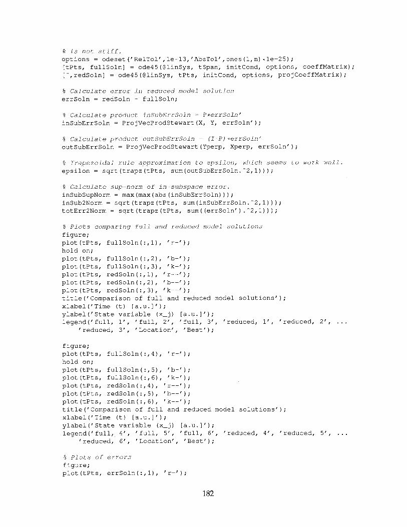
% is not stiff.options = odeset('RelTol',le-13,'AbsTol',ones(l,n)*le-25);[tPts, fullSoln] = ode45(@linSys, tSpan, initCond, options, coeffMatrix);

[~,redSoln] = ode45(@linSys, tPts, initCond, options, projCoeffMatrix);

% Calculate error in reduced model sol uton

errSoln = redSoln - fullSoln;

% Calculate product insubErrSoln = P*errSoln'

inSubErrSoln = ProjVecProdStewart(X, Y, errSoln');

% Calculate product out SubErrSon = (1 ..P)*errSoln'outSubErrSoln = ProjVecProdStewart(Yperp, Xperp, errSoln');

% 7Trape zCldal rule aprC)xima tion t~o epsilOn, whi ch sEEm.fs to work we]. .

epsilon = sqrt(trapz(tPts, sum(outSubErrSoln.^2,1)));

% Calculate sup-norm of in-subspace error.

inSubSupNorm = max(max(abs(inSubErrSoln)));

inSub2Norm = sqrt(trapz(tPts, sum(inSubErrSoln.^2,1)));

totErr2Norm = sqrt(trapz(tPts, sum((errSoln').^2,1)));

% Plots comparlng fuil and reduced model solutions

figure;

plot(tPts, fullSoln(:,l), 'r-');

hold on;

plot(tPts, fullSoln(:,2), 'b-');

plot(tPts, fullSoln(:,3), 'k-');

plot(tPts, redSoln(:,l), 'r--');

plot(tPts, redSoln(:,2), 'b--');

plot(tPts, redSoln(:,3), 'k--');

title('Comparison of full and reduced model soluti

xlabel('Time (t) [a.u.]');

ylabel('State variable (x-j) [a.u.]');

legend('full, 1', 'full, 2', 'full, 3', 'reduced,

'reduced, 3', 'Location', 'Best');

figure;plot(tPts, fullSoln(:,4), 'r-'

hold on;

plot(tPts, fullSoln(:,5), 'b-'

plot(tPts, fullSoln(:,6), 'k-'

plot(tPts, redSoln(:,4), 'r--'

plot(tPts, redSoln(:,5), 'b--'

plot(tPts, redSoln(:,6), 'k--'

title('Comparison of full and

xlabel('Time (t) [a.u.]');

ylabel('State variable (xj)

legend('full, 4', 'full, 5','reduced, 6', 'Location',

ons');

1', 'reduced, 2', ...

reduced model solutions');

a.u.]'full,'Best'

6', 'reduced, 4', 'reduced, 5',

% .ots o errorsfigure;plot(tPts, errSoln(:,l), 'r-');

182

hold on;plot(tPts, errSoln(:,2), 'b-');

plot(tPts, errSoln(:,3), 'k-');plot(tPts, inSubErrSoln(1,:), 'r--');

plot(tPts, inSubErrSoln(2,:), 'b--');

plot(tPts, inSubErrSoln(3,:), 'k--');title('Error in reduced model solution');xlabel('Time (t) [a.u.]');

ylabel('Error in state variable (ej) [a.u.]');

legend('j=l', 'j=2', 'j=3', 'j=l, in-subspace',...

'j=2, in-subspace', 'j=3, in-subspace','Location', 'Best');

figure;

plot(tPts, errSoln(:,4), 'r-');hold on;

plot(tPts, errSoln(:,5), 'b-');plot(tPts, errSoln(:,6), 'k-');

plot(tPts, inSubErrSoln(4,:), 'r--');

plot(tPts, inSubErrSoln(5,:), 'b--');plot(tPts, inSubErrSoln(6,:), 'k--');

title('Error in reduced model solution');xlabel('Time (t) [a.u.]');

ylabel('Error in state variable (e-j) [a.u.]');

legend('j=4', 'j=5', 'j=6', 'j=4, in-subspace',...

'j=5, in-subspace', 'j=6, in-subspace', 'Location', 'Best');

end

B.2 Python Implementation

The Python 2.7.3 [209] implementation requires the installation of NumPy 1.6.2

(or later) [152], SciPy 0.10.1 (or later) [93], and Matplotlib 1.0.0 (or later) [90]. An

attempt was made to keep the number of dependencies to a minimum. It is likely

that the Python code below will work with Python 2.6 (or later).

#!1 usr/bin/env python

import numpyimport scipy. integrate

import scipy.linalg

import matplotlib.pyplotimport math

import copy

def lin-sys(t, y, A):IF IF i

Purpose:

Auxiliary function encoding a linear ODE system for numerical integration.

183

Arguments:

t (float): time

y (1-D numpy.ndarray): statesA (2-D numpy.ndarray): square coefficient array, where A. shape[1] == len (y)

Returns:

f (1-D numpy.ndarray): right-hand side of ODE

# If y were a column vector, we would calculate the right.hand side as

# A * y. Instead, y is a row -vector (by default in numpy), so we calculate

t y * A^T} (as if we took the previous case, where y is a column vector,# and used (A * y)I{T} yJ T) * A^{T}f = numpy.dot(A, y)

return f

def calcerr boundsthm_4_1(epsilon, gamma, mu-bar, T, V, V~perp):if ry fr

Purpose:

Calculate the error bounds given in Theorem 4.1.

Arguments:

epsilon (float): \varepsilon in Theorem 4.1, bound on function 2-norm of

out-of-subspace error, \1\mathbf[e}_{c}\|_{2}

gamma (float): \gamma in Theorem 4.1, bound on Lipschitz constant of

W^{T} * A in directions corresponding to W_[\perp}, where \dot{y](t)= A * y(t)

mubar (float): \bar{\mu} in Theorem 4.1, bound on logarithmic norm ofW^{T} * A * V, where \dot{y) (t) = A*y(t)

T (float): end time of integration

V (2-D numpy.ndarray of floats): \mathbf{V) matrix in Theorem 4.1, basis

for range of projectorV perp (2-D numpy.ndarray of floats) : \mathbf[V}_\perp] matrix in

Theorem 4.1, basis for orthogonal complement of range of projector

Returns:

insub sup normbound (float): bound on the function sup-norm of the in-

subspace error, \|\mathbf{e}_{i}\|_{\infty} in Theorem 4.1

insub_2_normbound (float): bound on the function 2-norm of the in-

subspace error, \|\mathbf{e}_{i}\|_{2}

toterr_2_normbound (flooat): bound on the function 2-norm of the total

error, \|\mathbf{e} \|_2}

insub-sup-normbound = (epsilon * gamma

math.sqrt((math.exp(2 * mu_.bar * T) - 1) / (2 * mu bar)) *

numpy.linalg.norm(V, 2) * numpy.linalg.norm(V~perp, 2))

#ConvenJence iarable used to koId intermediate.:esuJt common to two# later expressionstwonormscaling-factor = (gamma * numpy.linalg.norm(V, 2) *

184

numpy.linalg.norm(Vperp, 2) * math.sqrt((math.exp(2 * mubar * T) - 1 - 2 * mubar * T) / (4 * mu-bar ** 2)))

insub_2_normbound = epsilon * twonormscaling-factortoterr_2_normbound = epsilon * (1 + twonorm-scaling_factor)

return (insubsupnormbound, insub_2_normbound, toterr_2_normbound)

def calc_XQRY-rep(range-basis, null-basis):If If ,,

Purpose:

Calculates the XQRY representation of a projection matrix and itscomplementary projection matrix, given a basis for the range and nullspace of the projection matrix. See G. W. (Pete) Stewart's "On theNumerical Analysis of Oblique Projectors", SIMAX, 2011 for additionaldetails.

Arguments:

range basis (2-D numpy.ndarray of floats): basis for range space ofprojection matrix

nullbasis (2-D numpy.ndarray of floats): basis for null space ofprojection matrix

Returns:

X (2-D numpy.ndarray of floats): orthonormal basis for range of projectorY (2-D numpy.ndarray of floats): orthonormal basis for range of transpose

of projectorN (2-D numpy.ndarray of floats): inv(Y^{T} * X)X-perp (2-D numpy.ndarray of floats): orthonormal basis whose span is

orthogonal to span(X)Y perp (2-D numpy.ndarray of floats): orthonormal basis whose span is

orthogonal to span (Y)Nc (2-D numpy.ndarray of floats): inv(X-perp^{T} * Y perp)

Assertion checks:None. Should check for consistency of matrix dimensions.

F1 ,, if

(n, k) = range basis.shape

# Calculate Petrov-Galerkin matrices and projector. Use C. W. (Pete)# Stewart's "On the Numerical Analysis of Oblique Projectors", SIMAX, 2011# to guide algorithms; in this case, the algorithms being used is (5.1).

# Q and R will be temporary variables used for the results of QR# tact o.r...zations.

# First, use QR actoi 1,zation to fnd ort.ogo120naL ratrices whose C.o]umns.span the des.reo subspaces. Use Stewart's nomenclature.

(Q, _) = scipy.linalg.qr(range basis)X = Q[:, O:k]X-perp = Q[:, k:]

185

# Yperp is a basis for the null space; Y is a basis for the -range of P^{Y)

(Q, _) = scipy.linalg.qr(nullbbasis)Y_perp = Q[:, O:k]

Y = Q[:, k:]

# Ca]culate .intermedare matrices for Stewart's XQRY representation.

M = numpy.dot(Y.transposeo, X)

(Q, R) = scipy.linalg.qr(M)N = numpy.linalg.solve(R, Q.transposeo)

M_c = numpy.dot(X-perp.transpose(), Y-perp)

(Q, R) = scipy.linalg.qr(M_c)N_c = numpy.linalg.solve(R, Q.transposeo)

return (X, Y, N, X-perp, Y-perp, N-c)

def calc_explicit-projector(X, Y, N):if if it

Purpose:

From their respective XQRY representations, calculate the projectionmatrix with range equal to span (X) and whose transpose has range span(Y).

Arguments:X (2-D numpy.ndarray of floats): orthonormal basis for range of projectorY (2-D numpy.ndarray of floats): orthonormal basis for range of transpose

of projector

N (2-D numpy.ndarray of floats): inv(Y^{T} * X)

Returns:

P (2-D numpy.ndarray of floats): projection matrix

Assertion checks:

None. Should check for consistency of matrix dimensions.

# Stewart warns against calculating projection matrices directLy, due to#f possibie numerical error, but .t is neeed for some performance metrICs,# (like the norm of P) .

P = numpy.dot(X, numpy.dot(N, Y.transposeo))

return P

def calcnormI_W rep(X, Y, N, Xperp, Yperp, Nc):

Purpose:

From their respective XQRY representations, calculate the V and

W corresponding to the projection matrix with range equal to

span(X) and whose transpose has range span(Y), such that the columns

of W are orthonormal (i.e., numpy.linalg.norm(W, 2) = 1). Also calculateWkperp and Vperp, corresponding to the complementary projection matrix,

such that the columns of WKperp are orthonormal (i.e.,numpy. linalg.norm (Wperp, 2) = 1) .

186

Arguments:


of projectorN (2-D numpy.ndarray of floats): inv(Y^{T} * X)

X perp (2-D numpy.ndarray of floats): orthonormal basis whose span isorthogonal to span (X)

Yperp (2-D numpy.ndarray of floats): orthonormal basis whose span isorthogonal to span (Y)

Nc (2-D numpy.ndarray of floats) : inv(Xperp^{T) * Y perp)

Returns:

V (2-D numpy.ndarray of floats): basis for range of projectorW (2-D numpy.ndarray of floats): orthonormal matrix such that ker(W^{T})

is null space of projector; V * W^{T} = projectorWPperp (2-D numpy.ndarray of floats): basis for rnage of complementary

projector, orthonormal matrixVperp (2-D numpy.ndarray of floats): matrix such that ker(Vperp^{T}) is

null space of complemntary projector; Wkperp * V1perp^{T} =

complementary projector

Assertion checks:

None; should make sure that matrix dimensions areconsistent, and that X, Y, and N are consistent, etc.

# XY representation of projector calculated using aorit-ham suggested at.#f bottorm of p. 323 in G. W. (Pete) Stewart's "On the Numerical Analysis of# Oblique Pro etOs.", S F MAX, 201.1

V = numpy.dot(X, N)

W= Y

V-perp = numpy.dot(X-perp, N-c.transpose()

W-perp = Y-perp

return (V, W, Vperp, Wperp)

def calc_norm_1_V_rep(X, Y, N, Xperp, Yperp, Nc):Vr I tr

Purpose:

From their respective XQRY representations, calculate the V and Wcorresponding to the projection matrix with range equal to span(X) andwhose transpose has range span(Y), such that the columns of V areorthonormal (i.e., numpy.linalg.norm(V, 2) = 1). Also calculate WPperp andV perp, corresponding to the complementary projection matrix, such thatthe columns of VXperp are orthonormal (i.e.,numpy. linalg.norm (V-perp, 2) = 1).

Arguments:


of projectorN (2-D numpy.ndarray of floats): inv(Y^{T} * X)

187

X-perp (2-D numpy.ndarray of floats): orthonormal basis whose span is

orthogonal to span(X)

Yperp (2-D numpy.ndarray of floats): orthonormal basis whose span is

orthogonal to span (Y)N_c (2-D numpy.ndarray of floats): inv(Xperp^{T} * Yperp)

Returns:

V (2-D numpy.ndarray of floats): orthonormal matrix, basis for range of

projectorW (2-D numpy.ndarray of floats): matrix such that ker(W^{T)) is null

space of projector; V * W^{T} = projector

WAperp (2-D numpy.ndarray of floats): basis for range of complementary

projector

V1perp (2-D numpy.ndarray of floats): orthonormal matrix such that

ker(Vperp^{T}) is null space of complementary projector;

WPperp * V1perp^{T} = projector

Assertion checks:None; should make sure that matrix dimensions are consistent, and that

X, Y, and N are consistent, etc.

if if it

# XY representation of projector calculated using algorithm suggested at

# bottom of 0. 323 in G. W. (Pete) Stewart's "On the Numerical Analysis of

# Oblique Projectors"r, S MA'1AX, 201.1.

V= XW = numpy.dot(N, Y.transposeo).transpose()

W-perp = numpy.dot(Yperp, Nc)

V-perp = X-perp.transpose()

return (V, W, V~perp, Wperp)

def calc_thm_4__consts(coeffmatrix, V, W, Wperp):

Purpose:

Calculate the constants that determine the error bounds in Theorem 4.1.

Arguments:

coeffmatrix (2-D numpy.ndarray of floats): A matrix in

\dot{y) (t) = A*y(t)V (2-D numpy.ndarray of floats): basis for range of projector

W (2-D numpy.ndarray of floats): matrix such that ker(W^{T}) is the null

space of the projector; V * W^[T) = projector

WPperp (2-D numpy.ndarray of floats): basis for range of complementary

projector

Returns:gamma (float): \gamma in Theorem 4.1, bound on Lipschitz constant of

W^{T} * A in directions corresponding to W_{\perp}, where \dot{y] (t)

= A * y(t)

mubar (float): \bar{\mu} in Theorem 4.1, bound on logarithmic norm of

W^{T} * A * V, where \dot{y) (t) = A * y(t)

188

Assertion checks:

None; should be consistency of dimensions of V, W, Wperp.

rr Fr IF

gamma = numpy.linalg.norm(numpy.dot(W.transpose(),numpy.dot(coeffmatrix, Wperp)), 2)

matrix = numpy.dot(W.transpose(, numpy.dot(coeffmatrix,V))

mubar = numpy.max(numpy.real(numpy.linalg.eigvals(

matrix + matrix.transposeo))) / 2

return gamma, mubar

def calcthm_4_4_consts(coeffmatrix, X, Y, Wperp):it FF FF

Purpose: Calculate the constants that determine the error bounds in

Theorem 4.4.

Arguments:

coeffmatrix (2-D numpy.ndarray of floats): A matrix in

\dot y] (t) = A*y(t)X (2-D numpy.ndarray of floats): orthonormal basis for range of projector

Y (2-D numpy.ndarray of floats): orthonormal basis for range of transpose

of projector

WKperp (2-D numpy.ndarray of floats): basis for range of complementary

projector

Returns:

gamma (float): \gamma in Theorem 4.4, bound on Lipschitz constant of

P * A in directions corresponding to W_{\perp}, where \dot{y}(t)

= A * y(t)

mubar (float): \bar[\mu} in Theorem 4.1, bound on logarithmic norm of

P * A, where \dot{y} (t) = A * y(t)

Assertion checks:None; should check consistency of dimensions of coeffmatrix, X, Y,W perp; check orthogonality of WPperp (should have 2-norm of 1).

if FF IF

proj-coeffmatrix = proj-vec-prod stewart(X, Y, coeff matrix)

gamma = numpy.linalg.norm(numpy.dot(proj-coeff-matrix, W perp))mubar = numpy.max(numpy.real(numpy.linalg.eigvals(

proj-coeffmatrix + proj-coeff matrix.transpose()))) / 2

return gamma, mubar

def pro jvecprod stewart (X, Y, v)Pr F sf

Purpose:

189

Calculate projector-vector product from an XQRY representation of a

projector using algorithm (5.2) in G. W. (Pete) Stewart's "On the

Numerical Analysis of Oblique Projectors", SIMAX, 2011.

Arguments:


of projector

v (1-D numpy.ndarray of floats): vector to be projected

Returns:

product (1-D numpy.ndarray of floats): P*v = projected vector

Assertion checks: None.

(Q, R) = scipy.linalg.qr(numpy.dot(Y.transpose(), X))

cl = numpy.dot(Y.transposeo, v)

c2 = numpy.dot(Q.transposeo, cl)

c3 = numpy.linalg.solve(R, c2)

product = numpy.dot(X, c3)

return product

def calcerrors(T, init-cond, coeffmatrix, X, Y, Xperp, Yperp):

Purpose:

Calculate solutions to the full and reduced models, plot these

solutions, and then calculate various errors in the reduced model.

Arguments:

T (float): end time for numerical integration

initcond (1-D numpy.ndarray of floats): initial condition for

numerical integration

coeffmatrix (2-D numpy.ndarray of floats): coefficient (A) matrix forlinear system, \dot{y](t) = A * y(t), n by n


of projector

X perp (2-D numpy.ndarray of floats): orthonormal basis whose span isorthogonal to span (X)

Yperp (2-D numpy.ndarray of floats): orthonormal basis whose span isorthogonal to span(Y)

Returns:

epsilon (float): function 2-norm of component of error in reduced modelsolution in null space of projection matrix

insub supnorm (float): function sup-norm of component of error inreduced model solution in range of projection matrix

insub_2_norm (float): function 2-norm of component of error in reducedmodel solution in range of projection matrix

toterr_2_norm (float): function 2-norm of total error in reduced modelsolution

190

soln_fig_1, soln-fig_2 (matplotlib.pyplot.Figure): plots of full andreduced model solutions

errfig l, err fig_2 (matplotlib.pyplot.Figure): plots of in-subspace and

total error

Assertion checks:None; check consistency of matrix dimensions.

if IV if

# Simulate system, emulatinq Rathinam and Petzold, SINUM, 2004.

t-begin = 0t_end = T

n_time-pts = 1000

t = numpy.linspace(t-begin, tend, ntimepts)

# Cal culat e prodi.ct proj coeffmatrix =P * coeff_matrixproj-coeffmatrix = proj-vec-prod stewart(X, Y, coeffjmatrix)

# Set up numerical iJnt.regrators. Note that the error tolerances are set# very tightly to decrease numerical error due to integration. Use 7th-order# explicit Runge-Kutta integration because systems are not stiff.fullsys = scipy.integrate.ode(linsys)fullsys.setjintegrator('dop853', atol=le-25, rtol=le-13, nsteps=10000000)fullsys.setjinitialvalue(initcond, 0)

fullsys.set-f-params(coeffmatrix)

red-sys = scipy.integrate.ode(linsys)red-sys.set-integrator('dop853', atol=le-25, rtol=le-3, nsteps=10000000)

red-sys.setinitialvalue(initcond, 0)

red-sys.set-f_params(proj-coeff matrix)

# Run integration loops; use numpy. vstack to avoid the need for copying# state of integrators.full soln = init cond

for point in t[l:]:

if not full-sys.successful(): break

full-sys.integrate(point)fullsoln = numpy.vstack((full_soln, full-sys.y))

redsoln = initcondfor point in t[l:]:

if not red-sys.successful(): break

red-sys.integrate(point)

redsoln = numpy.vstack((redsoln, red-sys.y))

# Calculate error in reduced model so. Uton

errsoln = redsoln - fullsoln

# Ca cula.e proCt In_ sub err_so = P * err_ so n { T}

insuberrsoln = projvecprodstewart(X, Y, errsoln.transposeO)

# Calculate product out_sub_err._soln = (I P) * err so1n ̂ T)outsuberrsoln = proj-vec-prod stewart(Y-perp, X-perp,

191

errsoln.transpose()

# Trapezoidal rule approximation to epsilon, which seems to work well.

epsilon = numpy.sqrt(numpy.trapz(numpy.sum(out-suberrsoln ** 2, axis=O), t))

# Caloulate remaining normsinsub-sup-norm = numpy.max(numpy.abs(in-suberr_soln))

insub_2_norm = numpy.sqrt(numpy.trapz(numpy.sum(in-suberrsoln ** 2, axis=O), t))

toterr_2_norm = numpy.sqrt(numpy.trapz(numpy.sum(err-soln.transpose() ** 2, axis=O), t))

# Plots oomparing full and reduced model solutionssoln-fig_1 = matplotlib.pyplot.figure()matplotlib.pyplot.plot(t, full soln[:, 0], 'r-')

matplotlib.pyplot.plot(t, full-soln[:, 1], 'b-')

matplotlib.pyplot.plot(t, full-soln[:, 2], 'k-')

matplotlib.pyplot.plot(t, red-soln[:, 0], 'r--')

matplotlib.pyplot.plot(t, red-soln[:, 1], 'b--')

matplotlib.pyplot.plot(t, red soln[:, 2], 'k--')

matplotlib.pyplot.title('Comparison of full and reduced model solutions')

matplotlib.pyplot.xlabel('Time (t) [a.u.]')

matplotlib.pyplot.ylabel('State variable (x-j) [a.u.]')

matplotlib.pyplot.legend( ('full, 1', 'full, 2', 'full, 3','reduced, 1', 'reduced, 2', 'reduced, 3'), loc='best')

soln-fig_2 = matplotlib.pyplot.figure()matplotlib.pyplot.plot(t, full-soln[:, 3], 'r-')

matplotlib.pyplot.plot(t, full-soln[:, 4], 'b-')

matplotlib.pyplot.plot(t, full-soln[:, 5], 'k-')

matplotlib.pyplot.plot(t, red soln[:, 3], 'r--')

matplotlib.pyplot.plot(t, red soln[:, 4], 'b--')

matplotlib.pyplot.plot(t, red-soln[:, 5], 'k--')

matplotlib.pyplot.title('Comparison of full and reduced model solutions')


matplotlib.pyplot.ylabel('State variable (x-j) [a.u.]')

matplotlib.pyplot.legend( ('full, 4', 'full, 5', 'full, 6','reduced, 4', 'reduced, 5', 'reduced, 6'), loc='best')

errfig_1 = matplotlib.pyplot.figure()matplotlib.pyplot.plot(t, err-soln[:, 0], 'r-')

matplotlib.pyplot.plot(t, err soln[:, 1], 'b-')

matplotlib.pyplot.plot(t, err-soln[:, 2], 'k-')matplotlib.pyplot.plot(t, insuberr-soln[0, :], 'r--')

matplotlib.pyplot.plot(t, insuberr-soln[l, :], 'b--')matplotlib.pyplot.plot(t, insuberr-soln[2, :], 'k--')

matplotlib.pyplot.title('Error in reduced model solution')

matplotlib.pyplot.xlabel('Time (t) [a.u.]')matplotlib.pyplot.ylabel('Error in state variable (ej) [a.u.]')

matplotlib.pyplot.legend( ('total, 1', 'total, 2', 'total, 3',

'in-subspace, 1', 'in-subspace, 2', 'in-subspace, 3'), loc='best')

errfig_2 = matplotlib.pyplot.figure()

192

matplotlib.pyplot.plot(t, err-soln[:, 3], 'r-')

matplotlib.pyplot.plot(t, err-soln[:, 4], 'b-')

matplotlib.pyplot.plot(t, err-soln[:, 5], 'k-')

matplotlib.pyplot.plot(t, in-suberr_soln[3, :], 'r--')

matplotlib.pyplot.plot(t, in-suberr_soln[4, :1, 'b--')

matplotlib.pyplot.plot(t, in-suberr_soln[5, :], 'k--')



matplotlib.pyplot.ylabel('Error in state variable (ej) [a.u.]')

matplotlib.pyplot.legend( ('total, 4', 'total, 5', 'total, 6',

'in-subspace, 4', 'in-subspace, 5', 'in-subspace, 6'), loc='best')

return (epsilon, insubsupnorm, in-sub_2_norm, tot err_2_norm,

solnfig_l, soln_fig_2, errfig_l, err-fig_2)

def comparison_of_models(coeffmatrix, range-basis, nullbasis, init-cond):

Purpose:

Integrates the linear system \dot{\mathbf{x}} = coeffmatrix * \mathbf{x},

and also integrates the projected system \dot{\hat{\mathbf{x}]} =\mathbf{P) * coeffmatrix * \hat{\mathbf{x]}. \mathbf [P} is a projection

matrix that has range equal to the space spanned by the columns ofrangebasis, and null space equal to the space spanned by nullbasis.

Arguments:

coeffmatrix (2-D numpy.ndarray of floats): square coefficient matrix of

linear ODE system; coeffmatrix.shape[O] == len(initcond)range-basis (2-D numpy.ndarray of floats): columns determine range space

of projection matrix; coeffmatrix.shape[O] == range-basis.shape[Oj

nullbasis (2-D numpy.ndarray of floats): columns determine null space ofprojection matrix; coeffmatrix.shape[0] == nullbasis.shape[O], andcoeff.matrix.shape[1] == (nullbasis.shape [1] + rangebasis.shape[1])

initcond (1-D numpy.ndarray of floats): initial condition for integration

Returns:

solnfig_1, soln-fig_2 (matplotlib.pyplot.Figure): plots of full andreduced model solutions

err fig_1, err fig_2 (matplotlib.pyplot.Figure): plots of in-subspace andtotal error

Assertion checks:None; doesn't check for consistency, although error checks could be addedlater. NOTE: Many plots assume that n = 6 (# of variables); these can begeneralized.

# GJet size of probLem and number of ranae basis vectors(n, k) = range basis.shape

#y Calculate Petrov-Galerk.in matrices and projector. Use G. W. (Pete)# St:"ew ar: Is "On the Numerical Analysis of Oblique Projectors", SIAlAX,# Vol. 32, No. 1, pp. 309-348 (2011), to guide algorithms.(X, Y, N, Xperp, Y-perp, Nc) = calc_XQRY-rep(range-basis, nullbasis)

193

#Stewart warns against calculating projection matrices directly, due to# possible numerical error, but here, it is needed for some performance

# metrics (the norm of P) .P = calc-explicit-projector(X, Y, N)

# Ciaculate V, W, Vperp, _perp where numpy. linalg.normh(W, 2)

nmpy.linalg.norm(Wiperp, 2) =1.

(V, W, Vperp, Wperp) = calcnorm__Wrep(X, Y, N, X-perp, Yperp, Nc)

# Calculate V, W, Vperp, WLperp where numpy.linaig.norm(V, 2)# numpy. linalg. norm (.perp, 2) = - .(Vprime,

W-prime,

V-prime-perp,

W-prime-perp) = calcnormlV-rep(X, Y, N, Xperp, Yperp, Nc)

# Calculate constant in Theorem 4.1 and Corollary 4.4:

Or ig inal/ c.ho.. ce of V, W, VZperp, W-perp(gamma, mu-bar) = calcthm_4_1_consts(coeff matrix, V, W, Wperp)

# Constants after change of basis for V, W, V_perp, and W perp

(gammaprime,

mubarprime) = calc_thm_4_1_consts(coefftmatrix, V~prime,W-prime, W-prime-perp)

# Corollary 4.4: Constants u sJ1ng projection matrix instead

(gamma-pro j,mubar-proj) = calc_thm_4_4_consts(coeffmatrix, X, Y, W-perp)

# Now, to simulate full and reduced system, emulating Rathinam and

# Petzold, "A New Look at Proper Orthogonal Decomposition ", SINUM,# Vol . 41, No. 5, pp. 1893.1925 (2004).

T = 5

(epsilon, in sub supnorm, in_sub_2_norm, toterr_2_norm,

solnfigj, soln_fig_2,

err-figj,

errfig_2) = calc_errors(T, init_cond, coeffmatrix,X, Y, X-perp, Y-perp)

# Cal culate error .bounos

(insubsupnorm bound,

insub_2_normbound,

toterr_2_normbound) = calcerrboundsthm_4_ (epsilon, gamma,

mu-bar, T, V, V~perp)

print '-----------------------------------------------------------'print 'Size of matrix A (n by n), n = {}'.format(n)

print 'Size of reduced order model, k = {}'.format(k)

print 'gamma = {}' .format (gamma)

print 'mubar = {}'.format(mu-bar)

print '2-norm of P = {}'.format(numpy.linalg.norm(P, 2))

print '2-norm of V = {}'.format(numpy.linalg.norm(V, 2))

194

print '2-norm of W = {}'.format(numpy.linalg.norm(W, 2))print 'gammaprime (gamma under change of basis) = {}'.format(gamma-prime)print 'mu-bar-prime (mubar under change of basis) = {}' .format(

mubarprime)print '2-norm of V-prime = {}'.format(numpy.linalg.norm(Vprime, 2))print '2-norm of Wprime = {}'.format(numpy.linalg.norm(W-prime, 2))print '2-norm of V-primeperp = {}'.format(numpy.linalg.norm(

V_prime-perp, 2))print 'gamma-proj (gamma using P) = {}'.format(gamma-proj)print 'mu-bar-proj (mu-bar using P) = {}'.format(mu-barproj)

print 'Condition number of N = {}'.format(numpy.linalg.cond(N))

print 'Using gamma and mubar:'print '2-norm of out-of-subspace error, epsilon = {}'.format (epsilon)print '2-norm of in-subspace error = {}'.format(insub_2_norm)print 'Bound on 2-norm of in-subspace error = {}'.format(

insub_2_normbound)print 'Sup-norm of in-subspace error = {}'.format(insubsup-norm)print 'Bound on sup-norm of in-subspace error = {}'.format(

insub-sup-norm bound)

print '2-norm of total error = {}'.format(tot-err_2_norm)print 'Bound on 2-norm of total error = {}'.format(toterr_2_normbound)print '-----------------------------------------------------------

return (solnfig_1, solnfig_2, errfigj, err-fig_2)

def mainfunction():FFF rf i

Purpose:

Main driver function.

Arguments:None.

Returns:

None.

if FF if

# Set problem sizen = 6

# Set the seed of the random number generator for reproducib-ility.numpy.random.seed(0)

numpy.random.rand(n)

# "A" matrix from Rathinam and Pet zold, "A New Look at Proper OrthogonalDecompo siton", SIN7M, Vol . 41, No. 5, pp. 18-93-1925 (2004).

petzoldA_1 = numpy.asarray([[-0.1, 0, 0],[0, -0.1732, 2],[0, -2, -0.1732]])

petzold_A_2 = numpy.asarray([[-1.0, 0, 0],[0, -1.226, -0.7080],[0, 0.7080, -1.226]])

petzold_A_12 = numpy.asarray([[0.3893, 0.5179, -1.543],

195

[1.390, 1.3, 0.8841],

[0.06293, -0.9078, -1.184]])

petzoldA = numpy.vstack((numpy.hstack((petzold_A1, petzold_A_12)),

numpy.hstack((numpy.zeros((3, 3)), petzoldA_2))))

# Use svmmetri zed Pet zoL matrix with spectrum shifted downward, so that# spectrum i.s real, and its Iogarithmlc 2-norm is negative. Set range

# basis to last three eigenvectors (which have nonzero entries in their

# last three components). Set null space equal to the first three standard

# Euclidean basis vectors.symmA = copy.copy(petzoldA)symmA[l, 2] = -2symmA[5, 4] = -0.7080symmA = symm_A - 2 * numpy.eye(n)

(eigen-val, eigen-vec) = numpy.linalg.eig(symmA)rangebasis = eigen-vec[:, 3:6]

nullbasis = numpy.vstack((numpy.zeros((3,3)), numpy.eye(3)))

# Generate random initial condition#ini t_cond = numpy. random.rand (n)

initcond = numpy.ones(n)

# Run case study on this coefficient matrix and choice of bases(example_lsoln_1, examplelsoln_2, example_1_err_1,

examplelerr_2) = comparison ofmodels(symmA,

range-basis, null-basis, initcond)

# Scale the upper right block of the symmet rized, shifted

# which corresonds to halving gamma in our bounds.

lower-gammaA = copy.copy(symmA)lowergammaA[0:3, 3:6] = .5 * symmA[0:3, 3:6](eigen-val, eigen-vec) = numpy.linalg.eig(lower-gammaA)

rangebasis = eigen-vec[:, 3:6]

# Run case study on coefficient.matrix 1or second example

(example_2_soln_1, example_2_soln_2, example_2_err_1,

example_2_err_2) = comparison ofmodels(lowergammaA,range-basis, null-basis, init_cond)

# Scale the lower right block of the symmetrized, shifted

# which corresponds to increasing mu in our bounds.highermuA = copy.copy(symmA)higher muA[3:6, 3:6] = .715 * symmA[3:6, 3:6]

(eigenval, eigen vec) = numpy.linalg.eig(higher-muA)

rangebasis = eigen-vec[:, 3:6]

# Run case study on coef.Ient mat ri.x for th .rd example(example_3_soln_1, example_3_soln_2, example_3_err_1,

example_3_err_2) = comparison ofmodels(highermuA,

range-basis, null-basis, init_cond)


P etz..d matrix,

Pet zold matrix

196

return

if _name_ == "V-main__mainfunction()

197

Appendix C


Chapter 4

Examples for Chapter 4 were implemented in both MATLAB r2012a [133] and in

Python 2.7.3 [209].

C.1 MATLAB Implementation

The MATLAB r2012a [133] implementation requires the installation of Sundials 2.4

(or later), and SundialsTB [85].

function IllustrativeCaseStudy()% Case study tht ses 7etzold and Rath4 in m's example in SINUM, 2004, but

z% uses a diferent reduced model to I.ust rate a more genera.. result

% Close al.].. plotsclose all;format long e;

% Get the default random number generation stream in MATLAB, and reset It-% for reproduc-ibiljty. See "Loren on the Art of MATLAB", November 5, 2008,% http: //blos .mathworks.com/loren/2008/// (continued on next line)% new-ways -with-random-numbers -part-streamO = RandStream('mt19937ar','Seed',0);RandStream.setDefaultStream(streamO);

% Size o. mat r.cesn 6;

% "A" matrix from Rathinam and Petzold, SINUM, 2004.

199

petzoldAl = [-0.1, 0, 0;

0, -0.1732, 2;

0, -2.0, -0.1732;];

petzoldA2 = [-1.0, 0, 0;

0, -1.226, -0.7080;

0, 0.7080, -1.226;];

petzoldA12 = [0.3893, 0.5179, -1.543;

1.390, 1.3, 0.8841;

0.06293, -0.9078, -1.184;];

petzoldA = [petzoldAl, petzoldA12;

zeros(3,3), petzoldA2];

% Block factors, used to make it so that gamma is determined by he upper% block and muBa.r is detbermitned by twe . ) ower block.upperBlockFactor = 2;lowerBlockFactor = 5;

% Modification of Petzold's coefficient matrix in order to make the example% more presentable.modell = [upperBlockFactor * petzoldAl, petzoldA12;

zeros(3,3), lowerBlockFactor * petzoldA2];

% Create reduced mode by zeroi ng out the upper right 3 by 3 bloc.k of the% Full model coeIff1 ent marrix.

redModell = modell;redModell(1:3,4:6) = zeros(3,3);

%d Random initial condition.% init~ond = rand (I, n) ;initCond = ones(1,6);

upperBlockFactor = 2;lowerBlockFactor = 10;

% Scaling factor for A.12 block so that epsi..Lon. .. s unchanged in modei2.couplingFactor 1.974500693397877;

% Modification or Pet zold' s coefficient matrix in order to make the examp I.e% more presentable.model2 = [upperBlockFactor * petzoldAl, couplingFactor * petzoldA12;


% Create reduced model by zeroing out the upper right 3 by 3 block of the- uL model coefi cient mat ri x.

redModel2 = model2;redModel2(1:3,4:6) = zeros(3,3);

upperBlockFactor = 1;

lowerBlockFactor = 5;

% Modification of Petzold's coefflcien matrix in order to make the example

200

% more presentable.model3 = [upperBlockFactor * petzoldAl, petzoldA12;


- Create reduced model by zeroi.ng out the unper right 3 by 3 block of the% fu 1 mode 1 c06?Ttcdent marx

redModel3 = model3;

redModel3(1:3,4:6) = zeros(3,3);

comparisonOfModels(modell, redModell, initCond);

comparisonOfModels(model2, redModel2, initCond);

comparisonOfModels (model3, redModel3, initCond);

end

uLIXi J T ar C s0 y sltuemgJ.i17.L'.1..7 Auxiiar fucio noding( a .11near1 ssEm for numerical n.egration

% here, A is the r2Oe.cuier matrix, y .s the state vector, and t .i.s time.function dy = linSys(t,y,A)dy = A * y;

end

function comparisonOfModels (fullMatrix, redMatrix, initCond)

6 Purose: Integrates the linear system \dot { \matxhb fx}} = fullkiatrix *

% \jathbf-x , adalso Ilntegrates the projected system

o \dnt { \ha{Imthbf 1 x}} = \Ithbt{! * uliMatrix * \hat{\mathbf{x}}.% \mathzf{ [ is a proj ection matrx that has range equal to the spaceC spann2d by he c'l.jumns of rangeBasis, and no]. space equa.] to the space

% nn by colJDum.lns nu Bas-is.Inpu i: a

trix = n by n, cefien matrix of .Linear ODE system; n

% s deter.ned' by sIze o matr.x

% redMatrix n by n, coefficient matrix of reduced model linear ODE

%sy,,s eminitond = by n, initial condition for integration; row vector

due to peculiarities of MATLAB syntax% Output: None to scope outside of call. Will output information relevant% to error bounds to term'i na1, either as text, or as plots.% Assert i. on checks: None ! 0oe sn' t check for con si stency, al though errorIi checks coumd be added ..ater. NOTE: many olots assume t n =; these% can be generai 1zed.

n = size(fullMatrix, 1);

% Calculate constants in Theorem 4.1 and Corollary 4.4:

% Oricinal choice of V, W, V'perp, Wperpgamma = norm(redMatrix);

muBar = max(real(eig(redMatrix + redMatrix')))/2;

% Now, to simulate systcnm, emulating Rathinam ano Petzold, SINUM, 2004tSpan = [0,5];

T = tSpan(2);

% Note that error .olerances seve to decrease numer ca error

% due to integration. Use 4th-order Runge.Kutta integration because system% is not stiff.

201

options = odeset('RelTol',le-13,'AbsTol',ones(1,n)*le-25);[tPts, fullSoln] = ode45(@linSys, tSpan, initCond, options, fullMatrix);

[~,redSoln] = ode45(@linSys, tPts, initCond, options, redMatrix);

% Calculate error in reduced model soLutionerrSoln = redSoln - fullSoln;

% CalCul ate both componen t 50 error.

outSubErrSoln = cumtrapz(tPts, (redMatrix - fullMatrix)*fullSoln', 2)';

inSubErrSoln = errSoln - outSubErrSoln;

% Trapezoldal rule approximation to epsilon, which seems to work well.epsilon = sqrt(trapz(tPts, sum(outSubErrSoln.^2,2)));

% CaLculate ninity norm of i..n-subspace error and compare to its predctIed9 bound.inSubInfNormBound = epsilon * gamma * ...

sqrt( (exp(2 * muBar * T) - 1) / (2 * muBar) );

inSubInfNorm = max(max(abs(inSubErrSoln)));

inSub2NormBound = epsilon * gamma * ...

sqrt( (exp(2 * muBar * T) - 1 - 2 * muBar * T) / (4 * muBar^2));inSub2Norm = sqrt(trapz(tPts, sum(inSubErrSoln.^2,2)));

% Calculate 2.norm of total error and compare to its predicted bound.% 2-norm of tota L r eror approximated us.i ng trapezoida. LetotErr2NormBound = epsilon * (1 + gamma * ...

sqrt( (exp(2 * muBar * T) - 1 - 2 * muBar * T) / (4 * muBar^2)) );totErr2Norm = sqrt(trapz(tPts, sum((errSoln').^2,1)));

%; Statements to check code, and results.fprintf(1, '-----------------------------------------------------------\n')

fprintf(l, 'Size of matrix A (n by n), n = %e\n', n)

fprintf(l, 'gamma = %e\n', gamma);fprintf(l, 'muBar = %e\n', muBar);

fprintf(l, '2-norm of truncating error, epsilon = %e\n', epsilon);

fprintf(l, '2-norm of propagating error = %e\n', inSub2Norm);

fprintf(l, 'Bound on 2-norm of propagating error = %e\n', inSub2NormBound);

fprintf(l, 'Sup-norm of propagating error = %e\n', inSubInfNorm);

fprintf(1, 'Bound on Sup-norm of propagating error = %e\n',

inSubInfNormBound);

fprintf(l, '2-norm of total error = %e\n', totErr2Norm);

fprintf(l, 'Bound on 2-norm of total error = %e\n', totErr2NormBound)

fprintf(1, '-----------------------------------------------------------\n')

% Plots:r r rsL:, .ncote that xI., x_2, and x_ 3 should bed -tferent bet ween the two

% models. Lso, notetha t he only nonzero components of he error shou d

% be e_ 1., e_2, and e_3.

figure;

plot(tPts, fullSoln(:,l), 'r-');

hold on;plot(tPts, fullSoln(:,2), 'b-');

202

plot(tPts, fullSoln(:,3), 'k-');

plot(tPts, redSoln(:,l), 'r--');plot(tPts, redSoln(:,2), 'b--');

plot(tPts, redSoln(:,3), 'k--');

title('Comparison of full and reduced model solutions');xlabel('Time (t) [a.u.]');

ylabel('State variable (x-j) [a.u.]');

legend('full, 1', 'full, 2', 'full, 3', 'reduced, 1', 'reduced, 2','reduced, 3', 'Location', 'Best');

figure;

plot(tPts, errSoln(:,l), 'r-');

hold on;

plot(tPts, errSoln(:,2), 'b-');

plot(tPts, errSoln(:,3), 'k-');

plot(tPts, inSubErrSoln(:,l), 'r--');

plot(tPts, inSubErrSoln(:,2), 'b--');

plot(tPts, inSubErrSoln(:,3), 'k--');

title('Error in reduced model solution');xlabel('Time (t) [a.u.]');

ylabel('Error in state variable (ej) [a.u.]');

legend('total, 1', 'total, 2', 'total, 3', 'propagating, 1','propagating, 2', 'propagating, 3', 'Location', 'Best');

end

C.2 Python Implementation

The Python 2.7.3 [209] implementation requires the installation of NumPy 1.6.2

(or later) [152], SciPy 0.10.1 (or later) [93], and Matplotlib 1.0.0 (or later) [90]. An

attempt was made to keep the number of dependencies to a minimum. It is likely

that the Python code below will work with Python 2.6 (or later).

#! /usr/bi n/env pyt hon

import numpy

import scipy. integrate

import matplotlib.pyplotimport math

import copy

def lin-sys(t, y, A):If ,, ,?

Purpose:

Auxiliary function encoding a linear ODE system for numerical integration.

Arguments:

t (float) : time

203

y (1-D numpy.ndarray): statesA (2-D numpy.ndarray): square coefficient array, where A.shape[l] == len(y)

Returns:f (1-D numpy.ndarray): right-hand side of ODE

If ,, if

f = numpy.dot(A, y)

return f

def comparison_of_models(full-matrix, redmatrix, initcond):

Purpose:Integrates the linear system \dot{\mathbf[x}} = fullmatrix * \mathbf{x},

and also integrates the reduced system \dot{\hat[\mathbf{x}}} =

redmatrix * \hat{\mathbf{x}}.

Arguments:

fullmatrix (2-D numpy.ndarray of floats): coefficient matrix of "full"

linear ODE system, square array

redmatrix (2-D numpy.ndarray of floats): coefficient matrix of "reduced"

linear ODE system, square array, redmatrix.shape == fullmatrix.shapeinit cond (1-D numpy.ndarray of floats): initial condition for integration,

row vector due to numpy syntax; len(init-cond) == fullmatrix.shape[1]

Returns:

soln fig (matplotlib.pyplot.Figure): figure containing plots of full and

reduced solution

errfig (matplotlib.pyplot.Figure): figure containing plots of total

error and propagating error

Assertion checks:

None; doesn't check for consistency, though error checks could be added later.

Many plots assume that len(init_cond) == 6; these could be generalized

# Ca.clate constants in Theorem 4.1 and Corol..ary 4.4:gamma = numpy.linalg.norm(red matrix, 2)mubar = numpy.max(numpy.real(

numpy.linalg.eigvals(redmatrix + redmatrix.transpose()))/2

# imulate system, emulating Rathinam and Pet-z ld, SINUM, 2004.

t_begin = 0t_end = 5

n_time-pts = 1000

t = numpy.linspace(t-begin, tend, ntime-pts)

#Set up numer-ca Integrat'ors. Note th.t he err or to..lerances are set

# very tight.1 to decrease numeri cal error due to in teg-rat ion. Use 7th-order

# exp/ ici t .Runge-.Kutta ntegrain because systems are not s .

fullsys = scipy.integrate.ode(linsys)full-sys.set-integrator('dop853', atol=le-25, rtol=le-13, nsteps=10000000)

204

full-sys.set-initial_value(initcond, 0)full-sys.set-f_params(fullmatrix)

red-sys = scipy.integrate.ode (linsys)red-sys.set-integrator('dop853', atol=le-25, rtol=le-3, nsteps=10000000)red-sys.setinitialvalue(initcond, 0)red-sys.set-f_params(redmatrix)

# Run int egra t.i.on loops; use numpy. vstac.k to avoid the need ror copying# state of integrators.full_soln = initcondfor point in t[l:]:

if not full-sys.successful(): break

full-sys.integrate(point)fullsoln = numpy.vstack((full_soln, full_sys.y))

redsoln = initcondfor point in t[l:]:

if not redsys.successful(): breakred-sys . integrate (point)redsoln = numpy.vstack((red-soln, red-sys.y))

# Calculate error in reduced model solutionerrsoln = redsoln - fullsoln

# Cal culate both components of e.ror

#out.sub_ err_ so.]n = scipy..interate. cumtrap (# numpy'. dot ((red matrix - ful..Lmatrix) , fu.. sCn . t ranspose () ) ,#f t, axi s=. ) . transpose()t_matrix = numpy.tile(t, (len(init_cond), 1)).transpose()outsuberrsoln = scipy.integrate.cumtrapz(

numpy.dot(fullsoln, (red-matrix - fullmatrix) .transpose()),t_matrix, axis=0)

outsuberrsoln = numpy.vstack( (numpy.zeros(len(initcond)),

outsuberrsoln))insuberrsoln = errsoln - outsuberrsoln

#t Trapezoda..7. rule aoprox.imation to epsIlon, which seems to work we..7epsilon = numpy.sqrt(numpy.trapz(

numpy.sum(out-suberrsoln ** 2, axis=l), t))

# Calculate infinity norm of in-subspace error and compare to its# predicted bound.T = tend

insubinfnormbound = (epsilon * gamma * math.sqrt(

(math.exp(2 * mubar * T) - 1) / (2 * mubar)))

insubinfnorm = numpy.max(numpy.abs(insuberr-soln))

insub_2_normbound = (epsilon * gamma * math.sqrt((math.exp(2 * mubar * T) - I - 2 * mubar * T) / (4 * mu-bar ** 2)))

insub_2_norm = math.sqrt(numpy.trapz(

numpy.sum(in_sub_errsoln ** 2, axis=1), t))

# Calculate 2.norm of total error and compare to its predicted bound.

205

#/ 2-norm of total error approximak-ed using trapezoidal rule.toterr_2_normbound = (epsilon * (1 + gamma * math.sqrt(

(math.exp(2 * mubar * T) - 1 - 2 * mubar * T) / (4 * mubar ** 2))))

toterr_2_norm = numpy.sqrt(numpy.trapz(

numpy.sum(err-soln ** 2, axis=1), t))

# Statements to check code, and resultsprint '-----------------------------------

print 'Size of matrix A (n by n), n = {}'.format(fullmatrix.shape[O])

print 'gamma = {}'.format(gamma)

print 'mubar = {}'.format(mu-bar)

print '2-norm of truncating error, epsilon = {)'.format(epsilon)

print '2-norm of propagating error = {}'.format(insub_2_norm)

print 'Bound on 2-norm of propagating error = {}'.format(

insub_2_normbound)

print 'Sup-norm of propagating error = {}'.format(in_subinf-norm)

print 'Bound on Sup-norm of propagating error = {}'.format(insubinfnormbound)

print '2-norm of total error = {}'.format(tot_err_2_norm)print 'Bound on 2-norm of total error = {}'.format(toterr_2_normbound)

print '-----------------------------------------------------------'

# Plots:# For the inputs given, x_1, x_2, and x_3 should be different between the# two models. Also, note that the only nonzero error components for these# inputs shoul.7d be e_ 1, e2, and e_ .3.soln-fig = matplotlib.pyplot.figure()matplotlib.pyplot.plot(t, fullsoln[:, 0], 'r-')matplotlib.pyplot.plot(t, fullsoln[:, 1], 'b-')matplotlib.pyplot.plot(t, fullsoln[:, 2], 'k-')

matplotlib.pyplot.plot(t, red-soln[:, 0], 'r--')matplotlib.pyplot.plot(t, red-soln[:, 1], 'b--')matplotlib.pyplot.plot(t, red soln[:, 2], 'k--')matplotlib.pyplot.title('Comparison of full and reduced model solutions')matplotlib.pyplot.xlabel('Time (t) [a.u.]')

matplotlib.pyplot.ylabel('State variable (x-j) [a.u.]')matplotlib.pyplot.legend( ('full, 1', 'full, 2', 'full, 3',

'reduced, 1', 'reduced, 2', 'reduced, 3'), loc='best')

errfig = matplotlib.pyplot.figure()matplotlib.pyplot.plot(t, err-soln[:, 0], 'r-')

matplotlib.pyplot.plot(t, err-soln[:, 1], 'b-')

matplotlib.pyplot.plot(t, err-soln[:, 2], 'k-')

matplotlib.pyplot.plot(t, insuberr-soln[:, 0], 'r--')matplotlib.pyplot.plot(t, insuberr-soln[:, 1], 'b--')

matplotlib.pyplot.plot(t, insuberr-soln[:, 2], 'k--')



matplotlib.pyplot.ylabel('Error in state variable (ej) [a.u.]')

matplotlib.pyplot.legend( ('total, 1', 'total, 2', 'total, 3','propagating, 1', 'propagating, 2', 'propagating, 3'), loc='best')

return soln_fig, errfig

206

def mainfunction():

Purpose:Main driver function.

Arguments:None

Returns:None.

,? I, it

problem size

the sed oft he .rando~m number genera or for rep.roucibi.I tyrandom.seed(0)

random.rand(n)

# "A" matrix from Rathinam and Pet zoLd,# Decomposition", SINUM, Vol.

petzold_A_1 = numpy.asarray([

petzold_A_2 = numpy.asarray([

petzold_A_12 = numpy.asarray(

41, No. 5, pp. 1893.1925 (2004).

[-0.1, 0, 0],

[0, -0.1732, 2],

[0, -2, -0.1732]])

[-1.0, 0, 0],[0, -1.226, -0.7080],[0, 0.7080, -1.226]])

[[0.3893, 0.5179, -1.543],

[1.390, 1.3, 0.8841],

[0.06293, -0.9078, -1.184]])

petzoldA = numpy.vstack(

(numpy.hstack( (petzoldA_1, petzoldA_12)),

numpy.hstack((numpy.zeros((3, 3)), petzoldA_2))))

# Block factors, used to make it so that gamma is determined by the upper# block and mu_bar is determined by the lower block.upper-blockfactor_1 = 2

lowerblockfactor_1 = 5

# Modification of Petzold and Rathinam's coefficient matrix in order to#i make the example more presentable.model_1 = numpy.vstack(

(numpy.hstack((upperblockfactor_1 * petzoldA_1, petzoldA_12)),numpy.hstack((numpy.zeros((3, 3)),lowerblockfactor_1 * petzold_A_2)))

Creat-te reduced model by zeroin. g out Lthe upper right 3 by 3 block of the# full model coefficien marrix

redmodel_1 = copy.copy(modelj1)redmodel_1[0:3,3:6] = numpy.zeros((3,3))

207

# Setn = 6

#Sm L.

numpy.numpy.

"A New Look at Proper Orth1ogonaL

# Random initial condltlon

#iini t_ cond = numPy.random. rand (n)

initcond = numpy.ones(n)

# Second set of block factors, used to make It so that gamma is determi.ed# by the upper block and mu bar and is determined by the I.1ower block.

# Gamma is doubled from the previous example. The coupling factor,which is a scalng factofor he A_12 b.ock, J.s app.!.li. ed so tha-t epsi .L. on

# is unchanged from the first example.upperblockfactor_2 = 2lowerblockfactor_2 = 10

coupling-factor_2 = 1.974500693397877

# Second example matrixmodel_2 = numpy.vstack(

(numpy.hstack((upper blockfactor_2 * petzold_A_1,coupling-factor_2 * petzold_A_12)),numpy.hstack((numpy.zeros((3, 3)), lowerblockfactor_2 * petzoldA_2)))

# Create reduced model from second example matrix by zeroing out the upper# right 3 by 3 block of the full model coefficient matkrixred_model_2 = copy.copy(model_2)redmodel_2[0:3, 3:6] = numpy.zeros((3,3))

# Third set of block factorsupperblockfactor_3 = 1

lower block factor_3 = 5

# Th et set ot block 1 actors to make the thrd exa.mplemodel_3 = numpy.vstack(

(numpy.hstack((upper-blockfactor_3 * petzold_A_1, petzoldA_12)),numpy.hstack((numpy.zeros((3, 3)),

lowerblockfactor_3 * petzoldA_2)))

# Create reduced model by zeroing out the upper right 3 by 3 block of the# 17u. model coeficient matrix

red_model_3 = copy.copy(model_3)

redmodel_3[0:3, 3:6] = numpy.zeros((3,3))

(solnfig_1,

err-fig_1) = comparisonofmodels(modelj, redmodel_1, init-cond)

(solnfig_2,err-fig_2) = comparisonofmodels(model_2, redmodel_2, initcond)(soln-fig_3,err-fig_3) = comparisonofmodels(model_3, redmodel_3, initcond)


return

if name == " main ":

mainfunction()

208

Appendix D

Implementation of Point-Constrained

Reaction Elimination and

Point-Constrained Simultaneous

Reaction and Species Elimination

Formulations in Chapter 5

A reference implementation of point-constrained reaction elimination and point-

constrained simultaneous reaction and species elimination is given in Python so

that it may be used as a basis for future reproducible research. In addition, unit

tests are also given to ensure that

D.1 Python Implementation

The Python 2.7.3 [209] implementation requires the installation of Cantera 2.0.0b3

(or later) [73], the Cantera Python interface, NumPy 1.6.2 (or later) [152], and PuLP

1.4.9 (or later) [135]. The PuLP package includes interfaces to multiple open-source

and proprietary solvers (including CPLEX and Gurobi). An attempt was made to

209

keep the number of dependencies to a minimum. It is likely that the Python code

below will work with Python 2.6 (or later).

# Re gui rement s# N1"umPy# Can era# PuLP

import numpyimport Canteraimport pulp

# OCtional :# in sta]led LB solvers (Gurobi, CPLEX, CBC, COIN)

def calccond_indep-data(idealgas):

Purpose: Calculate the condition-independent data needed for reactionelimination: the molar mass-stoichiometric matrix product

Arguments:

idealgas (Cant era.Solution): Cantera.Solut ion object specifyinga chemical reaction mechanism and the thermodynamic properties ofits constituent species

Returns:

massstoichprod (2-D numpy.ndarray of floats): product of diagonalmatrix of molar masses and stoichiometry matrix

molarmass = ideal-gas.molarMasses()stoichmatrix = (ideal-gas.productStoichCoeffs() -

ideal-gas.reactantStoichCoeffs()

massstoichprod = numpy.dot(numpy.diag(molar-mass), stoichmatrix)

return stoichmatrix, mass-stoichprod

def calc_conddep-data(state, idealgas):

Purpose: Calculate the condition-dependent data needed for reactionelimination:

- species mass enthalpies

- reaction rates

- mass-based constant pressure heat capacity

- mass density

Arguments:

state (list of floats, or 1-D numpy.ndarray of floats): Reactionconditions consisting of temperature and species mass fractions(in the order that they are specified in the Cantera mechanism).Temperature must be the first element in the system state list

210

(or 1-D numpy.ndarray); subsequent elements must be species mass

fractions, in the order that they are specified in the Cantera

mechanism.ideal-gas (Cantera.Solution): Cantera.Solution object specifying achemical reaction mechanism and the thermodynamic properties of itsconstituent species; uses state of ideal-gas to calculate properties

Returns:

rxnrate (1-D numpy.ndarray of floats): (row) vector of reaction rates

cp mass (float): mass-based constant pressure heat capacityenthalpy mass (1-D numpy.ndarray of floats): (row) vector of species

mass (or specific) enthalpies

rho (float): mass density

,, ,, If

idealbgas.setTemperature(state[0])

ideal gas.setMassFractions(state[1:])

rxnrate = ideal-gas.netRatesOfProgress()

cp-mass = ideal-gas.cp-mass()enthalpyMass = (ideal-gas.enthalpiesRT() *

ideal-gas.temperature() * Cantera.GasConstant)rho = ideal-gas.density()

return (rxnrate, cpmass, enthalpymass, rho)

def error_constraintdata(state, idealgas, massstoichprod, atol, rtol):

Purpose: Calculates all of the coefficients for the error constraintsin the point-constrained reaction and species elimination integerlinear programming formulations.

Arguments:

state (list of floats, or 1-D numpy.ndarray of floats): Reactionconditions consisting of temperature and species mass fractions(in the order that they are specified in the Cantera mechanism).Temperature must be the first element in the system state list(or 1-D numpy.ndarray); subsequent elements must be species massfractions, in the order that they are specified in the Canteramechanism.

ideal-gas (Cantera.Solution): Cantera. Solution object specifying achemical reaction mechanism and the thermodynamic properties of itsconstituent species; uses state of ideal-gas to calculate propertiesatol (1-D numpy.ndarray of floats): list of absolute tolerances;len(atol) == states.shape[l] == ideal-gas.nSpecies() + 1

rtol (1-D numpy.ndarray of floats): list of relative tolerances;len(rtol) == states.shape[1] == ideal-gas.nSpecies() + 1mass_stoichprod (2-D numpy.ndarray of floats): product of diagonalmatrix of molar masses and stoichiometry matrix

Returns:

coeffstemp (1-D numpy.ndarray of floats): coefficients for constraintson error in time derivative of temperature

211

coeffs-y (2-D numpy.ndarray of floats): coefficients for constraints on

on error in time derivatives of species mass fractionsrhstemp (float): right-hand side of constraints on error in time

derivative of temperaturerhsy (1-D numpy.ndarray of floats): right-hand side of constraints on

error in time derivatives of species mass fractions

Comments:

Could refactor this function to use the internal state of ideal_gas,

but the additional state argument was chosen to make the dependency

much more explicit.

if F If I

(rxnrate,

cp-mass,enthalpy-mass,

rho) = calc_conddepdata(state, ideal-gas)

coeffs-temp = numpy.dot(enthalpy-mass, numpy.dot(mass stoichprod,numpy.diag(rxnrate))) / (rho * cpmass)

tempdot = numpy.dot(coeffstemp, rxnrate)

rhs_temp = atol[] + rtol[O] * abs(tempdot)

ydot = numpy.dot(mass stoich-prod, rxnrate) / rhocoeffs-y = numpy.dot(mass-stoich-prod, numpy.diag(rxnrate)) / rho

rhsy = atol[l:] + numpy.dot(abs(ydot), numpy.diag(rtol[l:]))

return coeffs-temp, coeffsy, rhs-temp, rhs-y

def reactionelim(states, idealgas, atol, rtol,

lpsolver=pulp.solvers.GLPKCMD)):if rr 11

Purpose: Carries out reaction elimination (Bhattacharjee, et al.,

Comb Flame, 2003) on the mechanism specified in ideal-gas at the

conditions specified in states, using the absolute tolerances

specified in atol, and relative tolerances specified in rtol.

Arguments:

states (list of list of floats, or 2-D numpy.ndarray of floats):

each element of the outer list (or each row of the 2-Dnumpy.ndarray) corresponds to a system state (or condition).

Conditions consist of temperature and species mass fractions

(in the order that they are specified in the Cantera mechanism).Temperature must be the first element in the system state list

(or 1-D numpy.ndarray); subsequent elements must be species massfractions, in the order that they are specified in the Cantera

mechanism.

ideal_gas (Cantera.Solution): Cantera.Solution object specifyinga chemical reaction mechanism and the thermodynamic properties ofits constituent species

atol (list of floats or 1-D numpy.ndarray of floats): list ofabsolute tolerances; len(atol) == states.shape[l]

ideal-gas.nSpecies() + 1

212

rtol (list of floats or 1-D numpy.ndarray of floats): list of

relative tolerances; len(rtol) == states.shape[1] ==

ideal-gas.nSpecies() + 1lpsolver (pulp solver command): One of the solver commands listed

when running pulp.pulpTestAll(, such as:

pulp.solvers.PULPCBCCMD ()

pulp. solvers. CPLEXDLL ()

pulp. solvers . CPLEXCMD ()

pulp. solvers. CPLEXPY ()

pulp.solvers.COINCMD()

pulp. solvers. COINMPDLL()pulp.solvers.GLPKCMD()

pulp. solvers.XPRESS()

pulp. solvers. GUROBI()

pulp. solvers. GUROBICMD ()pulp. sol vers. PYGLPK ()

pulp.solvers.YAPOSIB()

These solvers also have optional arguments; see the PuLP documentation

for details. This argument allows one to change the solver and solver

options in the API call.

Returns:

z (list of ints, or 1-D numpy.ndarray of ints): binary variables

indicating which reactions should be kept, and which should be

eliminated

status (str): indicates the LP solver status; is one of "Not

Solved", "Infeasible", "Unbounded", "Undefined", "Optimal"

Warnings:This function alters the state of ideal-gas. If the state of that

object prior to calling this function needs to be preserved,

copy the object.

# Convert lists to numpy.ndarrays because the data structure is usefU.l

# for Lhe operators.atol = numpy.asarray(atol)

rtol = numpy.asarray(rtol)

# Set up the lists needed for indexingrxnlist = range(O, ideal-gas.nReactionso)rxnstrings = [str(n+l) for n in rxnlist]

# Instantite binary va ria bles for .nteger 7.nea.r programz-var = pulp.LpVariable.dicts('rxn_', rxn_strings, 0, 1, 'Integer')

# Inst antii1ate i nteger linear program and obj ct.iv fLuntionrxnelimILP = pulp.LpProblem("Reaction Elimination", pulp.LpMinimize)rxnelimILP += pulp.lpSum([z-var[s] for s

in rxnstrings]), "Number of reactions"

213

# Calculate condition -independent data and store(stoichmatrix, massstoich_prod) = calc_cond-indep-data(ideal-gas)ideal-gas.setPressure(Cantera.OneAtm)

# Add constraints loop over data pontsfor k in range(O, len(states)):

# Calculate cond.tion-dependent data(coeffs-temp, coeffs-y, rhstemp,rhs-y) = errorconstraint data(states[k],

ideal-gas, massstoichprod, atol, rtol)

# Add two temperature error constraints (lower, upper bounds)rxnelimILP += pulp.lpSum([coeffs-temp[i] *

(1 - zvar[rxn_strings[i]]) for i in rxn_list]) >= -rhstemp,"Temperature Error Lower Bound for Data Point " + str(k+1)

rxnelimILP += pulp.lpSum([coeffs-temp[i] *(1 - zvar[rxn_strings[i]]) for i in rxn_list]) <= rhs temp,"Temperature Error Upper Bound for Data Point " + str(k+l)

# Add constraints: Loop over species mass fractionsfor j in range(O, ideal-gas.nSpecieso):

# Add two species mass fraction error constraints (lower, upper# bounds)rxnelimILP += pulp.lpSum([coeffs-y[j, i] *

(1 - zvar[rxnstrings[i]]) for i in rxnjlist]) >= -rhsy[j],"Mass Fraction Species " + str(j+1) + \" Error Lower Bound for Data Point " + str(k+1)

rxnelimILP += pulp.lpSum([coeffs-y[j, i] *(1 - zvar[rxnstrings[i]]) for i in rxnjlist]) <= rhs_y[j],"Mass Fraction Species " + str(j+l) + \" Error Upper Bound for Data Point " + str(k+1)

# Solve integer linear programrxnelimILP.solve(solver=lpsolver)

# Return list of binary variables, solver statusz = [int(zvar[i].value()) for i in rxnstrings]#z = int (v. val ue () ) for v in rxn_ im_1LF.variables () 1return z, pulp.LpStatus[rxn-elimILP.status]

def reactionand-specieselim(states, idealgas, atol, rtol,

lpsolver=pulp.solvers.GLPKCMD)):y IF

Purpose: Carries out simultaneous reaction and specieselimination (Mitsos, et al.,Comb Flame, 2008;Mitsos, 2008, unpublished) on the mechanism specified inideal-gas at the conditions specified in states, using theabsolute tolerances specified in atol, and relative tolerancesspecified in rtol. Mitsos' unpublished formulation is used here,which decreases the number of integer variables in the mixed-integerlinear programming formulation, which decreases its run time comparedto the original formulation in Combustion and Flame.

214

Arguments:

states (list of list of floats, or 2-D numpy.ndarray of floats):

each element of the outer list (or each row of the 2-D

numpy.ndarray) corresponds to a system state (or condition).

Conditions consist of temperature and species mass fractions

(in the order that they are specified in the Cantera mechanism).

Temperature must be the first element in the system state list

(or 1-D numpy.ndarray); subsequent elements must be species mass

fractions, in the order that they are specified in the Cantera

mechanism.

ideal-gas (Cantera.Solution): Cantera.Solution object specifying

a chemical reaction mechanism and the thermodynamic properties of

its constituent species

atol (list of floats or 1-D numpy.ndarray of floats): list of

absolute tolerances; len(atol) == states.shape[l]

ideal-gas.nSpecies() + 1rtol (list of floats or 1-D numpy.ndarray of floats): list of

relative tolerances; len(rtol) == states.shape[l] ==

ideal-gas.nSpecies() + 1lpsolver (pulp solver command): One of the solver commands listed

when running pulp.pulpTestAll(), such as:

pulp. solvers. PULPCBCCMD()

pulp. solvers. CPLEXDLL ()

pulp.solvers.CPLEXCMD()

pulp. solvers. CPLEXPY()

pulp. solvers. COINCMD ()

pulp. solvers. COINMPDLL()pulp.solvers.GLPKCMD()

pulp. solvers.XPRESS()

pulp. solvers.GUROBI()

pulp. solvers. GUROBICMD ()pulp. solvers.PYGLPK()

pulp. solvers. YAPOSIB ()

These solvers also have optional arguments; see the PuLP documentation

for details. This argument allows one to change the solver and solver

options in the API call.

Returns:z (list of ints, or 1-D numpy.ndarray of ints): binary variables

indicating which reactions should be kept, and which should be

eliminated

w (list of ints, or 1-D numpy.ndarray of ints): binary variables

indicating which species should be kept, and which should be

eliminatedstatus (str): indicates the LP solver status; is one of "Not

Solved", "Infeasible", "Unbounded", "Undefined", "Optimal"

Warnings:

This function alters the state of ideal-gas. If the state of that

object prior to calling this function needs to be preserved,

copy the object.

215

,, F, Fr

# Convert lists to numpy.ndarrays because the data structure is useful# for the operators.atol = numpy.asarray(atol)rtol = numpy.asarray(rtol)

# Set up the lists needed for Indexingrxnlist = range(O, idealgas.nReactionso)

rxnstrings = [str(n+l) for n in rxnjlist]

specieslist = range(0, ideal-gas.nSpecieso)

species-strings = [str(n+l) for n in species-list]

# .nstant ate binary variables for Integer linear program

z_var = pulp.LpVariable.dicts('rxn_', rxn strings, 0, 1, 'Integer')w_var = pulp.LpVariable.dicts('species_', species-strings, 0, 1,

'Continuous')

# Instantiate integer linear program and objective functionrxnelimILP = pulp.LpProblem("Reaction Elimination", pulp.LpMinimize)rxnelimILP += pulp.lpSum([w-var[s] for s

in species-strings]), "Number of species"

# Calculate condi ti.on-ndePendent data and store(stoichmatrix, massstoich_prod) = calccond-indep-data(ideal-gas)ideal-gas.setPressure(Cantera.OneAtm)

# Add participation constraints from aierative Miutsos formulationfor j in range(0, ideal-gas.nSpecieso):

for i in range(0, ideal_gas.nReactions()):

if stoichmatrix[j, i] != 0:.rxnelimILP += \

w_var[species-strings[j]] - zvar[rxnstrings[i]] >= 0, \"Participation of species " + str(j+l) + \

and reaction " + str(i+1)

# Add error consAtracts: .oop over dat a po .-. nEtsfor k in range(0, len(states)):

# Calculate condition-dependent data(coeffstemp, coeffsy, rhstemp,

rhsy) = errorconstraint-data(states[k],idealgas, massstoichprod, atol, rtol)

#f Add two t.mperature error constraints (lower, upper bounds)

rxnelimILP += pulp.lpSum([coeffs-temp[i] *

(1 - z-var[rxn_strings[i]]) for i in rxnlist]) >= -rhs-temp, \"Temperature Error Lower Bound for Data Point " + str(k+1)

rxnelimILP += pulp.lpSum([coeffs-temp[i] *(1 - z-var[rxn_strings[i]]) for i in rxnlist]) <= rhs-temp, \"Temperature Error Upper Bound for Data Point " + str(k+1)

216

# Add constraints: Loop over species mass fractionsfor j in range(O, ideal-gas.nSpecieso):

#dd two species mass fraction error constraints (lower, upper#/ bounds)rxnelimILP += pulp.lpSum([coeffs-y[j, i] *

(1 - z_var[rxnstrings[i]]) for i in rxnlist]) >= -rhs_y[j],

"Mass Fraction Species " + str(j+l) + \" Error Lower Bound for Data Point " + str(k+l)

rxnelimILP += pulp.lpSum([coeffs-y[j, i] *(1 - z_var[rxnstrings[i]]) for i in rxnlist]) <= rhs-y[j],

"Mass Fraction Species " + str(j+l) + \" Error Upper Bound for Data Point " + str (k+l)

# So1v1 nteger . near program

rxn_elim_ILP.solve(solver=lpsolver)

# Return list of bi.na-ry variables, soIver statusz = [int(z-var[i].value()) for i in rxn-strings]

w = [int(wvar[j].value()) for j in species-strings]return z, w, pulp.LpStatus[rxnelimILP.status]

D.2 Python Unit Tests

Unit tests are provided here to ensure that any modifications to the code do not

break existing functionality, and to guard against errors in the Python implemen-

tation above.

import chemReduceimport Canteraimport unittestimport numpy

class TestCoeffIdentities (unittest .TestCase):def setUp(self):

#methodNa.me=' runTest', fi La_name'gri30.ctI-, temp=1i000,#press=Cantera.OneAtm, mass frac='CR4:.05, 02:.075, N2:.9', atol=le-6,#rtol=le.6) :

filename = 'gri3O.cti'temp = 1000

press = Cantera.OneAtmmassfrac = 'CH4:.05, 02:.075, N2:.9"'atol = le-6

rtol = le-6

# .InitIaize thermodynamic and kJnetI.c data and set staself.gas=Cantera.IdealGasMix('gri3.cti')

self.gas.set(T=temp, P=press, Y=mass-frac)

217

self.state = numpy.zeros(self.gas.nSpecies() + 1)

self.state[O] = self.gas.temperature()

self.state[l:] = self.gas.massFractions()

# Calculate condit..n-.ndependent data and store

(self.stoichmatrix,self.massstoich-prod) = chemReduce.calccondindep-data(self.gas)

# Calculate condtion-Jependent data and store(self. rxn-rate,

self.cp-mass,self.enthalpyjnass,

self.rho) = chemReduce.calc_cond-depdata(self.state, self.gas)

self.atol numpy.ones(self.gas.nSpecies() + 1) * atol

self.rtol = numpy.ones(self.gas.nSpecies() + 1) * rtol

self.floattol = le-6

def testrow_sums(self):It IF IF

Purpose: The sum of the entries in coeffs-temp should equal tempdot.

The sum of the entries in each row of coeffs-y should equal

numpy.asarray([ydotj) .transpose().

Arguments:

None

Returns:

None

I? Ifif,

(coeffstemp,coeffs_y,

rhstemp,rhsy) = chemReduce.errorconstraint_data(self.state,

sef.gas, self.mass_stoich-prod, self.atol, self.rtol)

# Test Identity for temperat. urerhs-temp_test = self.atol[O] + self.rtol[O] * numpy.sum(coeffs temp)self.assertAlmostEqual(numpy.max(abs(rhs temptest - rhs-temp)), 0,

delta=self.floattol)

# Test identity for each speciesrhs-y-test = numpy.zeros(self.gas.nSpecies()for j in range(0, self.gas.nSpecies()):

rhs_ytest[j] = (self.atol[j + 1] + self.rtol[j + 1]numpy.sum(coeffs-y[j,:1))

self.assertAlmostEqual(numpy.max(abs(rhs_y_test - rhsy)), 0,


def testcolsums(self):If f if

218

Purpose: The sum of over each column in coeffs y, where each row isscaled by enthalpy mass[j] / cpmass, should equal coeffst.

Arguments:

None

Returns:

None,v If it

(coeffs temp,

coeffs-y,

= chemReduce.errorconstraint_data(self.state,self.gas, self .mass_stoichprod, self.atol, self.rtol)

rowtotal = numpy.zeros(self.gas.nReactions()for j in range(O, self.gas.nSpecieso):

rowtotal += self.enthalpymass[j] * coeffsy[jl / self.cpmass

self.assertAlmostEqual(numpy.max(abs(rowtotal - coeffstemp)), 0,

delta = self.floattol)

def testnaivesummration(self):I, if ft

Purpose: Calculate the entries of coeffstemp, coeffs-y, rhs-temp,

rhsy using loops instead of vectorizing. Will be slow, but shouldyield same answer.

Arguments:

None

Returns:

NoneIF IF It

molarMass = self.gas.molarMasses()stoichMatrix = (self.gas.productStoichCoeffs() -

self.gas.reactantStoichCoeffs()

coeffs-yjloop = numpy.zeros((self.gas.nSpecies(,self.gas.nReactions()))

coeffs-temp-loop = numpy.zeros(self.gas.nReactionso)

for i in range(0, self.gas.nReactions()):coeffstempjloop[i] = numpy.sum(

[self.enthalpyMass[j] * molarMass[j] * stoichMatrix[j,i] *

self.rxn_rate[i] / (self.cp_mass * self.rho)

for j in range(0, self.gas.nSpecieso)])for j in range(0, self.gas.nSpecieso):

coeffs-y-loop[j,il = (molarMass[j] * stoichMatrix[j,i] *

self.rxn-rate[i] / self.rho)

temp-dot = numpy.sum(coeffstemp_loop)y-dot = numpy.sum(coeffs-yjloop, axis=l)

219

rhs-tempjloop = self.atol[O] + self.rtol[O] * abs(temp-dot)

rhs-yjloop = numpy.zeros(self.gas.nSpecieso)

for j in range(Q, self.gas.nSpecieso):

rhs_yjloop[j] = self.atol[j+1] + self.rtol[j+1] * abs(y-dot[j])

(coeffstemp,

coeffsy,

rhstemp,

rhsy) = chemReduce.errorconstraint_data(self.state,sef.gas, self.mass_stoich-prod, self.atol, self.rtol)

self.assertAlmostEqual(rhs-temp, rhstempjloop, delta=self.float-tol)

self.assertAlmostEqual(numpy.max(abs(rhsy - rhs_y_loop)), 0,


self.assertAlmostEqual(numpy.max(abs(coeffs-temp - coeffs-temp)), 0,


self.assertAlmostEqual(numpy.max(abs(coeffsy - coeffs-yjloop)), 0,


def testrunreaction-elim(self):

Purpose: Just run reactionelim on a simple test case to make sure

there are no syntax errors.

Arguments:

None

Returns:

None

chemReduce.reactionelim([self.state], self.gas, self.atol, self.rtol)

def testrunreaction-and-specieselim(self):

Purpose: Just run reactionandspecies-elim on a simple test case

to make sure there are no syntax errors.

Arguments:None

Returns:

None

If IF If

chemReduce.reactionandspecies-elim([self.state], self.gas,self.atol, self.rtol)

220

if -name- == ' main 'unittest.main()

#suite = unittest .Testui ()#t sul. tO. acdest( ( en t j t 7 (' rest naive__ summation'))

#sui te. addTest (t st. cfIdent it.es test sums'))#1su.ite.additest sn ('s ('test_ row_ sums'))#s1u te. aodest (Tests" ien- ies ('.testrun reaction elm' ) )#sui te addTest (Test Coe tidenti.ties ('test_.rureaction andisp)C.Leseliim'))

# sui te . debug ()

221

Bibliography

[1] Clean Air Act. Technical report, Code of Laws of the United States, Title 42,Chapter 85, 1970.

[2] The Montreal Protocol on Substances that Deplete the Ozone Layer. Techni-cal report, Ozone Secretariat United Nations Environment Programme, 1999.

[3] J. A kesson, K.-E. A rzen, M. Gafvert, T. Bergdahl, and H. Tummescheit.Modeling and optimization with Optimica and JModelica.orgLanguagesand tools for solving large-scale dynamic optimization problems. Comput-ers & Chemical Engineering, 34(11):1737-1749, November 2010.

[4] Joshua W Allen. PyDAS, 2010.

[5] loannis P. Androulakis. Kinetic mechanism reduction based on an integerprogramming approach. AIChE Journal, 46(2):361-371, February 2000.

[6] AC Antoulas and DC Sorensen. Projection methods for balanced model re-duction. Linear Algebra and Its Applications, 2004.

[7] A.C. Antoulas and DC Sorensen. Approximation of large-scale dynamicalsystems: An overview. In Large Scale Systems 2004: Theory and Applications(LSS'04): a Proceedings Volume from the 10th IFAC/IFORS/IMACS/IFIP Sym-posium, Osaka, Japan, 26-28 July 2004, volume 11, page 19. Elsevier for theInternational Federation of Automatic Control, 2005.

[8] AC Antoulas, DC Sorensen, and S. Gugercin. A survey of model reductionmethods for large-scale systems. In Structured Matrices in Mathematics, Com-puter Science, and Engineering: Proceedings of an AMS-IMS-SIAM Joint SummerResearch Conference, University of Colorado, Boulder, June 27-July 1, 1999, page193. Amer Mathematical Society, 2001.

[9] Athanasios Constantinos Antoulas. Approximation of Large-Scale DynamicalSystems. 2005.

[10] Michael Artin. Algebra. Prentice Hall, 1st edition, 1991.

[11] Uri Ascher and Linda Petzold. Computer Methods for Ordinary DifferentialEquations and Differential-Algebraic Equations. SIAM: Society for Industrialand Applied Mathematics, 1998.

223

[12] Uri M. Ascher and Linda R. Petzold. Computer Methodsfor Ordinary Differen-tial Equations and Differential-Algebraic Equations. SIAM: Society of Industrialand Applied Mathematics, 2000.

[13] A. Ben-Israel and T.N.E. Greville. Generalized inverses: Theory and applications.Springer Verlag, New York, 2nd edition, 2003.

[14] Gal Berkooz, Philip Holmes, and John L Lumley. The Proper OrthogonalDecomposition in the analysis of turbulent flows. Annual Review of FluidMechanics, 25:539-575, 1993.

[15] Luigi Carlo Berselli, Traian Iliescu, and William J Layton. Mathematics ofLarge Eddy Simulation of Turbulent Flows. Springer, 2010.

[16] Martin Berz and Kyoko Makino. Verified Integration of ODEs and FlowsUsing Differential Algebraic Methods on High-Order Taylor Models. ReliableComputing, 4:361-369, 1998.

[17] B Bhattacharjee, D A Schwer, P I Barton, and W H Green. Optimally-reducedkinetic models: reaction elimination in large-scale kinetic mechanisms. Com-bustion and Flame, 135:191-208, 2003.

[18] B. Bhattacharjee, D.A. Schwer, P.I. Barton, and W.H. Green. Optimally-reduced kinetic models: reaction elimination in large-scale kinetic mecha-nisms. Combustion and Flame, 135(3):191-208, 2003.

[19] M Bodenstein and H Lutkemeyer. The photochemical formation of hydro-gen bromide and the formation rate of the bromine molecules from theatoms. ZEITSCHRIFT FUR PHYSIKALISCHE CHEMIE-STOCHIOMETRIEUND, 114(3/4):208-236, December 1924.

[20] B. Bond. Parameterized model order reduction of nonlinear dynamical systems.Master's thesis, Massachusetts Institute of Technology, 2006.

[21] J. R. Bowen, A. Acrivos, and A. K. Oppenheim. Singular perturbation re-finement to quasi-steady state approximation in chemical kinetics. ChemicalEngineering Science, 18(3):177-188, March 1963.

[22] R.B. Brad, A.S. Tomlin, M. Fairweather, and J.F. Griffiths. The applicationof chemical reduction methods to a combustion system exhibiting complexdynamics. Proceedings of the Combustion Institute, 31(1):455-463, 2007.

[23] T. Bui-Thanh, K. Willcox, and 0. Ghattas. Model Reduction for Large-ScaleSystems with High-Dimensional Parametric Input Space. SIAM Journal onScientific Computing, 30(6):3270-3288, 2008.

[24] Y. Cao, S. Li, L. Petzold, and R. Serban. Adjoint Sensitivity Analysis forDifferential-Algebraic Equations (Part 2). SIAM Journal on Scientific Comput-ing, 24(3):1076-1099, 2003.

224

[25] Yang Cao and Linda Petzold. A posteriori error estimation and global er-ror control for ordinary differential equations by the adjoint method. SIAMJournal on Scientific Computing, 26(2):359-374, 2004.

[26] Makis Caracotsios and Warren E. Stewart. Sensitivity analysis of initial valueproblems with mixed odes and algebraic equations. Computers & ChemicalEngineering, 9(4):359-365, 1985.

[27] Kevin Carlberg, C. Bou-Mosleh, and Charbel Farhat. Efficient non-linearmodel reduction via a least-squares PetrovGalerkin projection and compres-sive tensor approximations. International Journalfor Numerical Methods in En-gineering, 86(2):155-181, 2011.

[28] D L Chapman and L K Underhill. The interaction of chlorine and hydrogen.The influence of mass. Journal of the Chemical Society Transactions, 103:496-508, 1913.

[29] S. Chaturantabut and Danny C Sorensen. A state space estimate for POD-DEIM Nonlinear Model Reduction. Technical report, 2010.

[30] S. Chaturantabut and D.C. Sorensen. Discrete empirical interpolation fornonlinear model reduction. In Decision and Control, 2009 held jointly with the2009 28th Chinese Control Conference. CDC/CCC 2009. Proceedings of the 48thIEEE Conference on, volume 339, pages 4316-4321. Ieee, 2004.

[31] Saifon Chaturantabut and Danny C Sorensen. Nonlinear model reductionvia discrete empirical interpolation. SIAM J. Sci. Comput., 32(5):2737-2764,2010.

[32] Saifon Chaturantabut and D.C. Sorensen. Application of POD and DEIMto Dimension Reduction of Nonlinear Miscible Viscous Fingering in PorousMedia. Math. Comput. Model. Dyn. Syst., to appear, 2009.

[33] Jacqueline H. Chen. Petascale direct numerical simulation of turbulent com-bustionfundamental insights towards predictive models. Proceedings of theCombustion Institute, 33(1):99-123, 2011.

[34] E Chiavazzo, IV Karlin, and AN Gorban. Comparison of invariant manifoldsfor model reduction in chemical kinetics. Communications in ComputationalPhysics, 2(5):964-992, October 2007.

[35] Yunfei Chu, Mitchell Serpas, and Juergen Hahn. State-preserving nonlinearmodel reduction procedure. Chemical Engineering Science, 66(17):3907-3913,September 2011.

[36] R. R. Coifman, I. G. Kevrekidis, S. Lafon, M. Maggioni, and B. Nadler. Dif-fusion maps, reduction coordinates, and low dimensional representation ofstochastic systems. Multiscale Model., 7(2):842-864, 2008.

225

[37] R. R. Coifman, S. Lafon, A. B. Lee, M. Maggioni, B. Nadler, F. Warner, andS. W. Zucker. Geometric diffusions as a tool for harmonic analysis and struc-ture definition of data: diffusion maps. Proceedings of the National Academy ofSciences of the United States of America, 102(21):7426-31, May 2005.

[38] Germund Dahlquist. Stability and Error Bounds in the Numerical Solution ofOrdinary Differential Equations. Phd thesis, Stockholm University, 1958.

[39] M J Davis and A S Tomlin. Spatial Dynamics of Steady Flames 2. Low-Dimensional Manifolds and the Role of Transport Processes. J. Phys. Chem.A, 112:7784-7805, 2008.

[40] Michael J Davis. Low-dimensional manifolds in reaction-diffusion equa-tions: {2. Numerical} analysis and method development. Journal of PhysicalChemistry A, 110:5257-5272, 2006.

[41] Michael J Davis and Rex T Skodje. Geometric investigation of low-dimensional manifolds in systems approaching equilibrium. Journal of Chem-ical Physics, 111(3):859-874, 1999.

[42] Michael J Davis and Alison S Tomlin. Spatial Dynamics of Steady Flames 1.Phase Space Structure and the Dynamics of Individual Trajectories. J. Phys.Chem. A, 112:7768-7783, 2008.

[43] MJ Davis. Low-dimensional manifolds in reaction-diffusion equations. 1.Fundamental aspects. J. Phys. Chem. A, 110(16):5235-5256, 2006.

[44] AP Davison. Automated Capture of Experiment Context for Easier Repro-ducibility in Computational Research. Computing in Science and Engineering,2012.

[45] Jan de Leeuw. Reproducible Research: The Bottom Line. Technical report,UCLA Department of Statistics Paper 2001031101, 2001.

[46] R.P. Dickinson and R.J. Gelinas. Sensitivity Analysis of Ordinary Differen-tial Equation Systems - A Direct Method. Journal of Computational Physics,21(2):123-143, 1976.

[47] Kai Diethelm. The Limits of Reproducibility in Numerical Simulation. Com-puting in Science & Engineering, 14(1):64-72, January 2012.

[48] R. Djouad, B. Sportisse, and N. Audiffren. Reduction of multiphase atmo-spheric chemistry. Journal of Atmospheric Chemistry, 46(2):131-157, 2003.

[49] David L. Donoho and Carrie Grimes. Hessian eigenmaps: Locally linearembedding techniques for high-dimensional data. Proceedings of the NationalAcademy of Sciences of the United States of America, 100(10):5591-5596, 2003.

226

[50] David L. Donoho, Arian Maleki, Inam Ur Rahman, Morteza Shahram, andVictoria Stodden. Reproducible Research in Computational Harmonic Anal-ysis. Computing in Science & Engineering, 11(1):8-18, January 2009.

[51] Eugene P. Dougherty and Herschel Rabitz. A computational algorithm forthe Green's function method of sensitivity analysis in chemical kinetics. In-ternational Journal of Chemical Kinetics, 11(12):1237-1248, December 1979.

[52] C. H. Edwards. Advanced Calculus of Several Variables. Dover Publications,revised edition, 1995.

[53] K. Edwards, TF Edgar, and VI Manousiouthakis. Reaction mechanismsimplification using mixed-integer nonlinear programming. Computers andChemical Engineering, 24(1):67-79, 2000.

[54] D Estep, V Ginting, D Ropp, JN Shadid, and S Tavener. An A posteriori-Apriori Analysis of Multiscale Operator Splitting. SIAM Journal on NumericalAnalysis, 46(3):1116-1146, 2008.

[55] D Estep, V Ginting, and S Tavener. A posteriori Analysis of a MultirateNumerical Methods for Ordinary Differential Equations. Technical report,2010.

[56] D Estep, S Tavener, and T Wildey. A posteriori Analysis and Improved Accu-racy for an Operator Decomposition Solution of a Conjugate Heat TransferProblem. SIAM Journal on Numerical Analysis, 46(4):2068-2089, 2008.

[57] Donald Estep. A Posteriori Error Bounds and Global Error Control for Ap-proximation of Ordinary Differential Equations. SIAM Journal on NumericalAnalysis, 32(1):1-48, 1995.

[58] Donald J Estep. Error Estimates for Multiscale Operator Decomposition ForMultiphysics Models. In Multiscale methods: bridging the scales in science andengineering, pages 305-388. Oxford University Press, USA, 2009.

[59] P. Faucher. Isopycnal empirical orthogonal functions (EOFs) in the Northand tropical Atlantic and their use in estimation problems. Journal of Geo-physical Research, 107(C8):1-17, 2002.

[60] W.F. Feehery, J.E. Tolsma, and P.I. Barton. Efficient sensitivity analysis oflarge-scale differential-algebraic systems. Applied Numerical Mathematics,25(1):41-54, October 1997.

[61] N Fenichel. Persistence and Smoothness of Invariant Manifolds for Flows.Indiana University Mathematics Journal, 21(3):193-226, 1971.

[62] N Fenichel. Asymptotic Stability with Rate Conditions. Indiana UniversityMathematics Journal, 23(12):1109-1137, 1974.

227

[63] N Fenichel. Geometric Singular Perturbation Theory for Ordinary Differen-tial Equations. Journal of Differential Equations, 31:53-98, 1979.

[64] M. Fjeld, 0. A. Asbj0 rnsen, and K. J. A str6m. Reaction invariants and theirimportance in the analysis of eigenvectors, state observability and control-lability of the continuous stirred tank reactor. Chemical Engineering Science,29(9):1917-1926, September 1974.

[65] Sergey Fomel and Jon F Claerbout. Reproducible Research. Computing inScience & Engineering, pages 5-7, 2009.

[66] Simon J Fraser. Slow manifold for a bimolecular association mechanism.Journal of Chemical Physics, 120:3075-3085, 2004.

[67] S.J. Fraser. The steady state and equilibrium approximations: A geometricalpicture. The Journal of Chemical Physics, 88(8):4732-4738, 1988.

[68] Juliana Freire and Claudio T Silva. Making Computations and PublicationsReproducible with VisTrails. Computing in Science and Engineering, 2012.

[69] S. Gadewar, M. F. Doherty, and M. F. Malone. A systematic method for re-action invariants and mole balances for complex chemistries. Computers &Chemical Engineering, 25(9-10):1199-1217, September 2001.

[70] Eric Garnier, Nikolaus Adams, and Pierre Sagaut. Large Eddy Simulation forCompressible Flows. Springer, 2009.

[71] Robert Gentleman and Duncan Temple Lang. Statistical Analyses and Re-producible Research. Journal of Computational and Graphical ... , 2007.

[72] S. K. Godunov. A difference method for numerical calculation of discontin-uous solutions of the equations of hydrodynamics. Matematicheskii Sbornik,47(89):271-306, 1959.

[73] D G Goodwin. An open-source, extensible software suite for CVD processsimulation. Chemical Vapor Deposition XVI and ... , 98(40):10147, 2003.

[74] A Gorban and I V Karlin. Method of invariant manifold for chemical kinet-ics. Chemical Engineering Science, 58(21):4751-4768, 2003.

[75] Alexander N Gorban and Iliya V Karlin. Invariant grids for reaction kinetics.Physica A: Statistical and Theoretical Physics, 333:106-154, 2004.

[76] D.A. Goussis and M. Valorani. An efficient iterative algorithm for the ap-proximation of the fast and slow dynamics of stiff systems. Journal of Com-putational Physics, 214(1):316-346, 2006.

[77] Thomas H Gronwall. Note on the derivatives with respect to a parameter ofthe solutions of a system of differential equations. The Annals of Mathematics,20(4):292-296, 1919.

228

[78] John Guckenheimer and Philip Holmes. Nonlinear Oscillations, DynamicalSystems, and Bifurcations of Vector Fields. Springer, New York, 2002.

[79] B Haasdonk and M. Ohlberger. Efficient Reduced Models and A-PosterioriError Estimation for Parametrized Dynamical Systems by Offline/OnlineDecomposition. Mathematical and Computer Modelling of Dynamical Systems,(1):1-17, 2011.

[80] Bernard Haasdonk and Mario Ohlberger. Reduced basis method for finitevolume approximations of parametrized linear evolution equations. ESAIM:Mathematical Modelling and Numerical Analysis, 42(2):277-302, March 2008.

[81] Bernard Haasdonk and Mario Ohlberger. Efficient reduced models for pa-rameterized dynamical systems by offline/online decomposition. In Proc.MATHMOD 2009, 6th Vienna International Conference on Mathematical Mod-elling, 2009.

[82] Bernard Haasdonk, Mario Ohlberger, and Gianluigi Rozza. A Reduced BasisMethod for Evolution Schemes with Parameter-Dependent Explicit Opera-tors. Electronic Transactions on Numerical Analysis, 32:145-161, 2008.

[83] Ernst Hairer, Syvert P No rsett, and Gerhard Wanner. Solving Ordinary Dif-ferential Equations I: Nonstiff Problems. Springer, Berlin, Germany, second revedition, 2000.

[84] Gary W. Harrison. Dynamic models with uncertain parameters. volume 1of Proceedings of the First International Conference on Mathematical Modeling,pages 295-304, 1977.

[85] Alan C Hindmarsh, Peter N Brown, Keith E Grant, Steven L Lee, Radu Ser-ban, D A N E Shumaker, and Carol S Woodward. SUNDIALS: Suite of Non-linear and Differential / Algebraic Equation Solvers. 31(3):363-396, 2005.

[86] C. Homescu, L.R. Petzold, and R. Serban. Error estimation for reduced-ordermodels of dynamical systems. SIAM Review, 49(2):277-299, 2006.

[87] C. Homescu, L.R. Petzold, and R. Serban. Error estimation for reduced-order models of dynamical systems. SIAM Journal on Numerical Analysis,43(4):1693-1714, 2006.

[88] Bill Howe. Virtual Appliances, Cloud Computing, and Reproducible Re-search. Computing in Science & Engineering, 14(4):36-41, July 2012.

[89] H. Huang, M. Fairweather, J.F. Griffiths, A.S. Tomlin, and R.B. Brad. A sys-tematic lumping approach for the reduction of comprehensive kinetic mod-els. Proceedings of the Combustion Institute, 30(1):1309-1316, January 2005.

[90] JD Hunter. Matplotlib: A 2D graphics environment. Computing in Science &Engineering, pages 90-95, 2007.

229

[91] Barbara R. Jasny, Gilbert Chin, Lisa Chong, and Sacha Vignieri. Again, andAgain, and Again.... Science, 334(December):2011, 2011.

[92] Christopher Jones. Geometric singular perturbation theory. In DynamicalSystems, Lecture Notes in Mathematics,, pages 44-118. 1995.

[93] Eric Jones, Travis Oliphant, Pearu Peterson, and Others. SciPy: Open SourceScientific Tools for Python, 2001.

[94] W Jones and S Rigopoulos. Rate-controlled constrained equilibrium: For-mulation and application to nonpremixed laminar flames. Combustion andFlame, 142(3):223-234, 2005.

[95] H.G. Kaper and T.J. Kaper. Asymptotic analysis of two reduction methodsfor systems of chemical reactions. Physica D: Nonlinear Phenomena, 165(1-2):66-93, 2002.

[96] James C. Keck. Rate-controlled constrained-equilibrium theory of chemi-cal reactions in complex systems. Progress in Energy and Combustion Science,16(2):125-154, 1990.

[97] James C. Keck and David Gillespie. Rate-controlled partial-equilibriummethod for treating reacting gas mixtures. Combustion and Flame, 17(2):237-241, October 1971.

[98] I G Kevrekidis, A E Deane, G E Karniadakis, and S A Orszag. Low-dimensional models for complex geometry flows: Application to groovedchannels and circular cylinders. Physics of Fluids A, 3(10):2337-2354, 1991.

[99] David J Knezevic. Reduced Basis approximation and a posteriori error es-timates for a Multiscale Liquid Crystal Model. Mathematical and ComputerModelling of Dynamical Systems, 2010.

[100] Mark a. Kramer. Nonlinear principal component analysis using autoassocia-tive neural networks. AIChE Journal, 37(2):233-243, February 1991.

[101] K Kunisch and S Volkwein. Control of the Burgers equation by a reduced-order approach using proper orthogonal decomposition. Journal of Optimiza-tion Theory and Applications, 102(2):345-371, 1999.

[102] K Kunisch and S Volkwein. Galerkin Proper Orthogonal DecompositionMethods for a General Equation in Fluid Dynamics. SIAM Journal on Nu-merical Analysis, 40:492-515, 2002.

[103] S H Lam. Using CSP to understand complex chemical kinetics. CombustionScience and Technology, 89(5):375-404, 1993.

[104] SH Lam and DA Goussis. The CSP method for simplifying kinetics. Interna-tional Journal of Chemical Kinetics, 26(4):461-486, 1994.

230

[105] J. Lang and J G Verwer. On Global Error Estimation and Control for InitialValue Problems. SIAM Journal on Scientific Computing, 27(4):21, 2007.

[106] Oliver F. Lange and Helmut Grubmuiller. Full correlation analysis of confor-mational protein dynamics. Proteins: Structure, Function, and Bioinformatics,pages 1294-1312, 2007.

[107] JC Lee, HN Najm, S. Lefantzi, J. Ray, M. Frenklach, M. Valorani, andDA Goussis. A CSP and tabulation-based adaptive chemistry model. Com-bustion Theory and Modelling, 11(1):73-102, 2007.

[108] J.M. Lee. Introduction to smooth manifolds. Springer Verlag, New York, 2003.

[109] Patrick A Legresley and Juan J Alonso. Dynamic Domain Decompositionand Error Correction for Reduced Order Models. In 41st Aerospace SciencesMeeting and Exhibit, 2003.

[110] Randall J LeVeque, Ian M Mitchell, and Victoria Stodden. Reproducible Re-search for Scientific Computing: Tools and Strategies for Changing the Cul-ture. Computing in Science & ... , pages 13-17, 2012.

[111] RJ LeVeque. Python Tools for Reproducible Research on Hyperbolic Prob-lems. Computing in Science & Engineering, pages 19-27, 2009.

[112] G. Li. A lumping analysis in mono- or/and bimolecular reaction systems.Chemical Engineering Science, 39(7-8):1261-1270, 1984.

[113] G. Li and H. Rabitz. A General Analysis of Exact Lumping in ChemicalKinetics. Chemical engineering science, 44(6):1413-1430, 1989.

[114] G. Li and H. Rabitz. A General Analysis of Approximate Lumping in Chem-ical Kinetics. Chemical engineering science, 45(4):977-1002, 1990.

[115] G. Li and H. Rabitz. A general lumping analysis of a reaction system coupledwith diffusion. Chemical engineering science, 46(8):2041-2053, 1991.

[116] G. Li and H. Rabitz. Determination of constrained lumping schemes fornonisothermal first-order reaction systems. Chemical Engineering Science,46(2):583-596, 1991.

[117] G. Li and H. Rabitz. New approaches to determination of constrained lump-ing schemes for a reaction system in the whole composition space. ChemicalEngineering Science, 46(1):95-111, 1991.

[118] Y Lin and M Stadtherr. Validated solutions of initial value problems forparametric ODEs. Applied Numerical Mathematics, 57(10):1145-1162, October2007.

231

[119] T. Lo vais, P. Amneus, F. Mauss, and E. Mastorakos. Comparison of automaticreduction procedures for ignition chemistry. Proceedings of the CombustionInstitute, 29(1):1387-1393, 2002.

[120] Michel Loeve. Probability Theory. Van Nostrand, 1955.

[121] T Lu and C Law. On the applicability of directed relation graphs to the re-duction of reaction mechanisms. Combustion and Flame, 146(3):472-483, 2006.

[122] T Lu and C Law. A criterion based on computational singular perturbationfor the identification of quasi steady state species: A reduced mechanism formethane oxidation with NO chemistry. Combustion and Flame, 154(4):761-774,2008.

[123] T Lu and C Law. Strategies for mechanism reduction for large hydrocarbons:n-heptane. Combustion and Flame, 154(1-2):153-163, 2008.

[124] T. Lu and C.K. Law. Systematic approach to obtain analytic solutions of quasisteady state species in reduced mechanisms. Journal of Physical Chemistry A,110(49):13202-13208, December 2006.

[125] T. Lu and C.K. Law. Toward accommodating realistic fuel chemistry in large-scale computations. Progress in Energy and Combustion Science, 35(2):192-215,2009.

[126] Tianfeng Lu and Chung K. Law. A directed relation graph method for mech-anism reduction. Proceedings of the Combustion Institute, 30(1):1333-1341, Jan-uary 2005.

[127] Tianfeng Lu and Chung K. Law. Linear time reduction of large kinetic mech-anisms with directed relation graph: n-Heptane and iso-octane. Combustionand Flame, 144(1-2):24-36, January 2006.

[128] D.J. Lucia, P.I. King, P.S. Beran, and M.E. Oxley. Reduced order modeling fora one-dimensional nozzle flow with moving shocks. In 15th AIAA Computa-tional Fluid Dynamics Conference, volume paper, 2001.

[129] X. Ma and G.E. Karniadakis. A low-dimensional model for simulating three-dimensional cylinder flow. Journal of Fluid Mechanics, 458:181-190, 2002.

[130] Ulrich Maas and Steven B Pope. Simplifying chemical kinetics: Intrinsiclow-dimensional manifolds in chemical composition space. Combustion andFlame, 88:239-264, 1992.

[131] T. Maly and L.R. Petzold. Numerical methods and software for sensitiv-ity analysis of differential-algebraic systems. Applied Numerical Mathematics,20(1-2):57-79, August 1996.

232

[132] S Margolis. Time-dependent solution of a premixed laminar flame. Journalof Computational Physics, 27(3):410-427, June 1978.

[133] MATLAB. Version 7.14.0 (R2012a). The MathWorks Inc., Natick, Mas-sachusetts, 2012.

[134] Jill P Mesirov. Accessible Reproducible Research. Science, 327(January):415-416, 2010.

[135] Stuart Mitchell, Stuart Mitchell Consulting, Michael 0 Sullivan, and lainDunning. PuLP: A Linear Programming Toolkit for Python. 2011.

[136] A M Mitsos. Alternative Formulation for Species Elimination. Technicalreport, RWTH Aachen, Aachen, Germany, 2008.

[137] Alexander Mitsos, Geoffrey M Oxberry, Paul I Barton, and William H Green.Optimal automatic reaction and species elimination in kinetic mechanisms.Combustion and Flame, 155:118-132, 2008.

[138] Parviz Moin and Krishnan Mahesh. Direct Numerical Simulation: A Tool inTurbulence Research. Annual Review of Fluid Mechanics, 30(1):539-578, Jan-uary 1998.

[139] Ramon E. Moore, R. Baker Kearfott, and Michael J. Cloud. Introduction toInterval Analysis. Society of Industrial and Applied Mathematics, 2009.

[140] R.E. Moore. Methods and applications of interval analysis. Society for IndustrialMathematics, Philadelphia, 1987.

[141] K R Mnller, S Mika, G Ratsch, K Tsuda, and B Schdlkopf. An introductionto kernel-based learning algorithms. IEEE transactions on neural networks /apublication of the IEEE Neural Networks Council, 12(2):181-201, January 2001.

[142] J Munkres. Analysis on Manifolds. Westview Press, 1st edition, 1990.

[143] B Nadler, S Lafon, R Coifman, and I Kevrekidis. Diffusion maps, spectralclustering and reaction coordinates of dynamical systems. Applied and Com-putational Harmonic Analysis, 21(1):113-127, July 2006.

[144] J. Nafe and U. Maas. A general algorithm for improving ILDMs. CombustionTheory and Modelling, 6(4):697-709, 2002.

[145] T. Nagy and T. Turanyi. Reduction of very large reaction mechanisms us-ing methods based on simulation error minimization. Combustion and Flame,156(2):417-428, February 2009.

[146] M Neher, KR Jackson, and NS Nedialkov. On Taylor Model Based Integra-tion of ODEs. SIAM Journal on Numerical ... , 45(1):236-262, 2007.

233

[147] Arnold Neumaier. Interval Methods for Systems of Equations. Cambridge Uni-versity Press, 2008.

[148] N Nguyen. A posteriori error estimation and basis adaptivity for reduced-basis approximation of nonaffine-parametrized linear elliptic partial differ-ential equations. Journal of Computational Physics, 227(2):983-1006, December2007.

[149] PH Nguyen. Complexity of Free Energy Landscapes of Peptides Revealedby Nonlinear Principal Component Analysis. Proteins: Structure, Function,and Bioinformatics, 913(October):898-913, 2006.

[150] Regents of the University of California. The BSD 3-Clause License. Web site.

[151] Miles S. Okino and Michael L. Mavrovouniotis. Simplification of Mathemat-ical Models of Chemical Reaction Systems. Chemical Reviews, 98(2):391-408,April 1998.

[152] Travis E. Oliphant. Python for Scientific Computing. Computing in Science &Engineering, 9(3):10-20, 2007.

[153] 0 0 Oluwole, P I Barton, and W H Green. Obtaining accurate solutionsusing reduced chemical kinetic models: a new model reduction method formodels rigorously validated over ranges. Combustion Theory and Modelling,11(1):127-146, 2007.

[154] 0 0 Oluwole, B Bhattacharjee, J E Tolsma, P I Barton, and W H Green. Rig-orous valid ranges for optimally reduced kinetic models. Combustion andFlame, 146(1-2):348-365, 2006.

[155] Geoffrey M. Oxberry. State-space error bounds for projection-based reducedmodel ODEs. 2012.

[156] Geoffrey M. Oxberry, Paul I. Barton, and William H. Green. Projection-basedmodel reduction in combustion. 2012.

[157] Roger Peng. Reproducible Research in Computational Science. Science,334(December):1226-1227, January 2011.

[158] Roger D. Peng and Sandrah P. Eckel. Distributed Reproducible ResearchUsing Cached Computations. Computing in Science & Engineering, 11(1):28-34, January 2009.

[159] P. Pepiot-Desjardins and H. Pitsch. An efficient error-propagation-basedreduction method for large chemical kinetic mechanisms. Combustion andFlame, 154(1-2):67-81, July 2008.

[160] Linda Petzold and Wenjie Zhu. Model Reduction for Chemical Kinetics: AnOptimization Approach. AIChE Journal, 45(4):869-886, 1999.

234

[161] Heinz Pitsch. Large-Eddy Simulation of Turbulent Combustion. Annual Re-view of Fluid Mechanics, 38(1):453-482, January 2006.

[162] Thierry Poinsot, Sebastien Candel, and Arnaud Trouve. Applications of di-rect numerical simulation to premixed turbulent combustion. Progress inEnergy and Combustion ... , 21(95):531-576, 1995.

[163] N. Ramdani, N. Meslem, and Y Candau. A Hybrid Bounding Method forComputing an Over-Approximation for the Reachable Set of Uncertain Non-linear Systems. IEEE Transactions on Automatic Control, 54(10):2352-2364, Oc-tober 2009.

[164] A Rapaport and D Dochain. Interval observers for biochemical processeswith uncertain kinetics and inputs. Mathematical Biosciences, 193(2):235-253,February 2005.

[165] M. Rathinam and L.R. Petzold. A new look at proper orthogonal decompo-sition. SIAM Journal on Numerical Analysis, 41(5):1893-1925, 2004.

[166] Z Ren, S B Pope, A Vladimirsky, and J M Guckenheimer. The invariant con-strained equilibrium edge preimage curve method for the dimension reduc-tion of chemical kinetics. Journal of Chemical Physics, 124(11):114111(1-10),2006.

[167] Z. Ren and S.B. Pope. The use of slow manifolds in reactive flows. Combus-tion and Flame, 147(4):243-261, 2006.

[168] Z. Ren and S.B. Pope. Reduced description of complex dynamics in reactivesystems. J. Phys. Chem. A, 111(34):8464-8474, 2007.

[169] M. Rewienski and J. White. A trajectory piecewise-linear approach to modelorder reduction and fast simulation of nonlinear circuits and micromachineddevices. IEEE Transactions on Computer-Aided Design of Integrated Circuits andSystems, 22(2):155-170, February 2003.

[170] M Rewienski and J White. Model order reduction for nonlinear dynamicalsystems based on trajectory piecewise-linear approximations. Linear Algebraand its Applications, 415(2-3):426-454, June 2006.

[171] C. Rhodes, M. Morari, and S. Wiggins. Identification of low order mani-folds: Validating the algorithm of Maas and Pope. Chaos: An InterdisciplinaryJournal of Nonlinear Science, 9(1):108-123, 1999.

[172] W. Richardson, L. Volk, KH Lau, SH Lin, and H. Eyring. Application of thesingular perturbation method to reaction kinetics. Proceedings of the NationalAcademy of Sciences, 70(5):1588-1592, 1973.

235

[173] Anthony Rossini and Friedrich Leisch. Literate Statistical Practice. TechnicalReport March 2003, University of Washington Biostatistics Working PaperSeries 194, Seattle, WA, USA, 2003.

[174] Marc R Roussel and Simon J Fraser. Geometry of the steady-state approxima-tion: Perturbation and accelerated convergence methods. Journal of ChemicalPhysics, 93(2):1072-1081, 1990.

[175] Marc R Roussel and Simon J Fraser. On the geometry of transient relaxation.Journal of Chemical Physics, 94(11):7106-7113, 1991.

[176] M.R. Roussel and S.J. Fraser. Invariant manifold methods for metabolicmodel reduction. Chaos: An Interdisciplinary Journal of Nonlinear Science,11(1):196-206, 2001.

[177] S. T. Roweis. Nonlinear Dimensionality Reduction by Locally Linear Em-bedding. Science, 290(5500):2323-2326, December 2000.

[178] G. Rozza, D.B.P. Huynh, and A.T. Patera. Reduced basis approximation anda posteriori error estimation for affinely parameterized elliptic coercive par-tial differential equations. Archives of Computational Methods in Engineering,15:229-275, 2008.

[179] Yousef Saad. Iterative Methods for Sparse Linear Systems Second Edition. SIAM:Society for Industrial and Applied Mathematics, 2003.

[180] Pierre Sagaut. Large Eddy Simulation for Incompressible Flows: An Introduction.Springer, third edition, 2005.

[181] Bernhard Schblkopf, Alexander Smola, and Klaus-Robert Muller. NonlinearComponent Analysis as a Kernel Eigenvalue Problem. Neural Computation,10(5):1299-1319, July 1998.

[182] Matthias Schwab, Martin Karrenbach, and Jon Claerbout. Making scientificcomputations reproducible. Computing in Science & ... , 2(6):61-67, 2000.

[183] D.A. Schwer, J.E. Tolsma, W.H. Green, and P.I. Barton. On upgrading thenumerics in combustion chemistry codes. Combustion and Flame, 128(3):270-291, 2002.

[184] Douglas A Schwer, Pisi Lu, William H Green, and Viriato Semiao. Aconsistent-splitting approach to computing stiff steady-state reacting flowswith adaptive chemistry. Combustion Theory and Modelling, 7:383-399, 2003.

[185] Radu Serban, Chris Homescu, and Linda R Petzold. The effect of prob-lem perturbations on nonlinear dynamical systems and their reduced-ordermodels. SIAM J. Sci. Comput., 29(6):2621-2643, 2007.

236

[186] Valeria Simoncini and Daniel B Szyld. Interpreting IDR as a Petrov-GalerkinMethod. Society, 32(4):1898-1912, 2010.

[187] Adam B. Singer and Paul I. Barton. Bounding the Solutions of ParameterDependent Nonlinear Ordinary Differential Equations. SIAM Journal on Sci-entific Computing, 27(6):2167, 2006.

[188] M.A. Singer and W.H. Green. Using adaptive proper orthogonal decompo-sition to solve the reactiondiffusion equation. Applied Numerical Mathematics,59(2):272-279, 2009.

[189] S Singh, J M Powers, and S Paolucci. On slow manifolds of chemically reac-tive systems. The Journal of Chemical Physics, 117(4):1482-1496, 2002.

[190] R.D. Skeel. Thirteen Ways to Estimate Global Error. Numerische Mathematik,48(1):1-20, 1986.

[191] Rex T Skodje and Michael J Davis. Geometrical Simplification of ComplexKinetic Systems. Journal of Physical Chemistry A, 105:10356-10365, 2001.

[192] Gustaf S6derlind. The logarithmic norm. History and modern theory. BITNumerical Mathematics, 46(3):631-652, August 2006.

[193] B. Sportisse and R. Djouad. Use of proper orthogonal decomposition for thereduction of atmospheric chemical kinetics. Journal of Geophysical Research-Atmospheres, 112(D6):D06303, 2007.

[194] B Srinivasan, M Amrhein, and D Bonvin. Reaction and Flow Vari-ants/Invariants in Chemical Reaction Systems with Inlet and Outlet Streams.AIChE Journal, 44(8):1858-1867, 1998.

[195] GW Stewart. On the numerical analysis of oblique projectors. SIAM Journalon Matrix Analysis and Applications, 32(1):309-348, 2011.

[196] Victoria Stodden. The Legal Framework for Reproducible Scientific Re-search: Licensing and Copyright. Computing in Science & Engineering,11(1):35-40, January 2009.

[197] Victoria Stodden. Reproducible Research: Tools and Strategies for ScientificComputing. Computing in Science & Engineering, pages 11-12, 2012.

[198] Victoria Stodden, David Donoho, Sergey Fomel, Michael Friedlander,Mark Gerstein, Randall J LeVeque, Ian Mitchell, Lisa Larrimore Ouellette,Chris Wiggins, Nicholas W Bramble, Patrick 0 Brown, Vincent J Carey,Laura DeNardis, Robert Gentleman, J Daniel Gezelter, Alyssa Goodman,Matthew G Knepley, Joy E Moore, Frank A Pasquale, Joshua Rolnick,Michael Seringhaus, and Ramesh Subramanian. Reproducible Research: Ad-dressing the need for data and code sharing in computational science. Journalof Computing Science and Engineering, 2010.

237

[199] G. Strang. On the construction and comparison of difference schemes. SIAMJournal on Numerical Analysis, 5(3):506-517, 1968.

[200] Gilbert Strang. Introduction to Linear Algebra. Wellesley Cambridge Press, 4thedition, 2009.

[201] H F Stripling, M Anitescu, and M L Adams. A Generalized Adjoint Frame-work for Sensitivity and Global Error Estimation in Time-Dependent Nu-clear Reactor Simulations. Technical Report 979, Preprint ANL/MCS-P1963-1011, Mathematics and Computer Science Division, Argonne National Lab-oratory, 2011.

[202] J B Tenenbaum, V de Silva, and J C Langford. A global geometric frame-work for nonlinear dimensionality reduction. Science (New York, N.Y.),290(5500):2319-23, December 2000.

[203] Alison S Tomlin, Tamas Turinyi, and Michael J Pilling. Mathematical toolsfor the construction, investigation and reduction of combustion mechanisms.In Comprehensive Chemical Kinetics, Volume 35: Low-Temperature Combustionand Autoignition, chapter 4, pages 293-437. Elsevier, 1997.

[204] J. Toth, G. Li, H. Rabitz, and A.S. Tomlin. The effect of lumping and expand-ing on kinetic differential equations. SIAM Journal on Applied Mathematics,57(6):1531-1556, 1997.

[205] Lloyd N. Trefethen and David Bau. Numerical Linear Algebra. Society forIndustrial and Applied Mathematics, 1997.

[206] M. Valorani, H.N. Najm, and D.A. Goussis. CSP analysis of a transient flame-vortex interaction: time scales and manifolds. Combustion and Flame, 134(1-2):35-53, 2003.

[207] Mauro Valorani and Dimitris A Goussis. Explicit Time-Scale Splitting Algo-rithm for Stiff Problems: Auto-ignition of Gaseous Mixtures behind a SteadyShock. Journal of Computational Physics, 169:44-79, 2001.

[208] Mauro Valorani, Dimitris A Goussis, Francesco Creta, and Habib N Najm.Higher order corrections in the approximation of low-dimensional mani-folds and the construction of simplified problems with the CSP method. Jour-nal of Computational Physics, 209:754-786, 2005.

[209] Guido van Rossum. The Python Programming Language, 1991.

[210] loan Vlad. Reproducibility in computer-intensive sciences. Ad Astra, 1(2):1-2, 2002.

[211] K.V. Waller and P.M. Makila. Chemical reaction invariants and variants andtheir use in reactor modeling, simulation, and control. Industrial & Engineer-ing Chemistry Process Design and Development, 20(1):1-11, 1981.

238

[212] H Wang and M Frenklach. Detailed reduction of reaction mechanisms forflame modeling. Combustion and Flame, 87(3-4):365-370, December 1991.

[213] J. Wei and J.C.W. Kuo. A lumping analysis in monomolecular reaction sys-tems. Industrial Engineering and Chemistry Fundamentals, 8(1):114-123, 1969.

[214] Kilian Q. Weinberger and Lawrence K. Saul. Unsupervised Learning of Im-age Manifolds by Semidefinite Programming. International Journal of Com-puter Vision, 70(1):77-90, May 2006.

[215] Charles K. Westbrook, Yasuhiro Mizobuchi, Thierry J. Poinsot, Phillip J.Smith, and Jtirgen Warnatz. Computational combustion. Proceedings of theCombustion Institute, 30(1):125-157, January 2005.

[216] Rowand Wilson and OSS Watch. The Modified BSD License - An Overview.Web site, May 2012.

[217] D. Wirtz and Bernard Haasdonk. Efficient a-posteriori error estimation fornonlinear kernel-based reduced systems. Outlook, 2(2010):48, 2011.

[218] Pedro E. Zadunaisky. On the estimation of errors propagated in the numer-ical integration of ordinary differential equations. Numerische Mathematik,71(1):20-39, March 1976.

[219] A. Zagaris, HG Kaper, and TJ Kaper. Analysis of Computational SingularPerturbation Reduction Method for Chemical Kinetics. Journal of NonlinearScience, 14(1):59-91, 2004.

[220] A. Zagaris, H.G. Kaper, and T.J. Kaper. Fast and slow dynamics for the com-putational singular perturbation method. Multiscale Model. Simul., 2(4):613-638, 2004.

[221] X.L. Zheng, T.F. Lu, and C.K. Law. Experimental counterflow ignition tem-peratures and reaction mechanisms of 1,3-butadiene. Proceedings of the Com-bustion Institute, 31(1):367-375, January 2007.

[222] OC Zienkiewicz, RL Taylor, and P Nithiarasu. The Finite Element Method forFluid Dynamics. Butterworth-Heinemann, sixth edition, 2005.

239

Establishing Global Error Bounds for Model Reduction in ...

Documents

Transcript of Establishing Global Error Bounds for Model Reduction in ...