HAL Id: hal-03155810https://hal.archives-ouvertes.fr/hal-03155810

Submitted on 2 Mar 2021

HAL is a multi-disciplinary open accessarchive for the deposit and dissemination of sci-entific research documents, whether they are pub-lished or not. The documents may come fromteaching and research institutions in France orabroad, or from public or private research centers.

L’archive ouverte pluridisciplinaire HAL, estdestinée au dépôt et à la diffusion de documentsscientifiques de niveau recherche, publiés ou non,émanant des établissements d’enseignement et derecherche français ou étrangers, des laboratoirespublics ou privés.

Fluid flow distribution optimization for minimizing thepeak temperature of a tubular solar receiver

Min Wei, yilin Fan, Lingai Luo, Gilles Flamant

To cite this version:Min Wei, yilin Fan, Lingai Luo, Gilles Flamant. Fluid flow distribution optimization for mini-mizing the peak temperature of a tubular solar receiver. Energy, Elsevier, 2015, 91, pp.663-677.�10.1016/j.energy.2015.08.072�. �hal-03155810�

1

Wei, M., Fan, Y., Luo, L., & Flamant, G. (2015). Fluid flow distribution optimization for minimizing 1 the peak temperature of a tubular solar receiver. Energy, 91, 663–677. 2

https://doi.org/10.1016/j.energy.2015.08.072 3

4

5

Fluid Flow Distribution Optimization for Minimizing the Peak 6

Temperature of a Tubular Solar Receiver 7

Min WEIa, Yilin FANa, Lingai LUOa*, Gilles FLAMANTb 8 a Laboratoire de Thermocinétique de Nantes, UMR CNRS 6607, Polytech' Nantes – 9

Université de Nantes, La Chantrerie, Rue Christian Pauc, BP 50609, 44306 Nantes Cedex 03, 10 France 11

b Laboratoire Matériaux, Procédés et Energie Solaire (PROMES), UPR CNRS 8521, 7 rue du 12 Four Solaire, 66120 Font-Romeu Odeillo, France 13

14

Abstract 15

High temperature solar receiver is a core component of solar thermal power plants. However, 16 non-uniform solar irradiation on the receiver walls and flow maldistribution of heat transfer 17 fluid inside the tubes may cause the excessive peak temperature, consequently leading to the 18 reduced lifetime. This paper presents an original CFD-based evolutionary algorithm to 19 determine the optimal fluid distribution in a tubular solar receiver for the minimization of its 20 peak temperature. A pressurized-air solar receiver comprising of 45 parallel tubes subjected to 21 a Gaussian-shape net heat flux absorbed by the receiver is used for study. Two optimality 22 criteria are used for the algorithm: identical outlet fluid temperatures and identical 23 temperatures on the centerline of the heated surface. The influences of different filling 24 materials and thermal contact resistances on the optimal fluid distribution and on the peak 25 temperature reduction are also evaluated and discussed. 26

Results show that the fluid distribution optimization using the algorithm could minimize the 27 peak temperature of the receiver under the optimality criterion of identical temperatures on 28 the centerline. Different shapes of optimal fluid distribution are determined for various filling 29 materials. Cheap material with low thermal conductivity can also meet the peak temperature 30 threshold through optimizing the fluid distribution. 31

32

Keywords: Flow maldistribution; High temperature solar receiver; Peak temperature; 33 Evolutionary algorithm; Optimality criterion 34

35

36

*Corresponding author. Tel.: +33 240683167; Fax: +33 240683141. E-mail address: lingai.luo@univ-nantes.fr

2

1. Introduction 1

Concentrated Solar Power (CSP) plants are expected to play an important role in the energetic 2 scenarios for more efficient use of renewable energy and for the reduced emission of 3 greenhouse gases [1, 2]. It is estimated that the CSP would contribute up to 11% of the global 4 electricity production in year 2050 [3, 4]. 5

In a CSP tower plant, the high temperature solar receiver installed at the top of the tower 6 absorbs and transforms the concentrated solar irradiation delivered from heliostats into heat 7 and then transfers it to a heat transfer fluid. The amount of heat carried by the heat transfer 8 fluid will be used in a downstream thermodynamic cycle to allow electricity generation. The 9 solar receiver, being a key component of CSP systems accounting for about 15% of the total 10 investment [5], has a decisive influence on the overall efficiency of the plant. 11

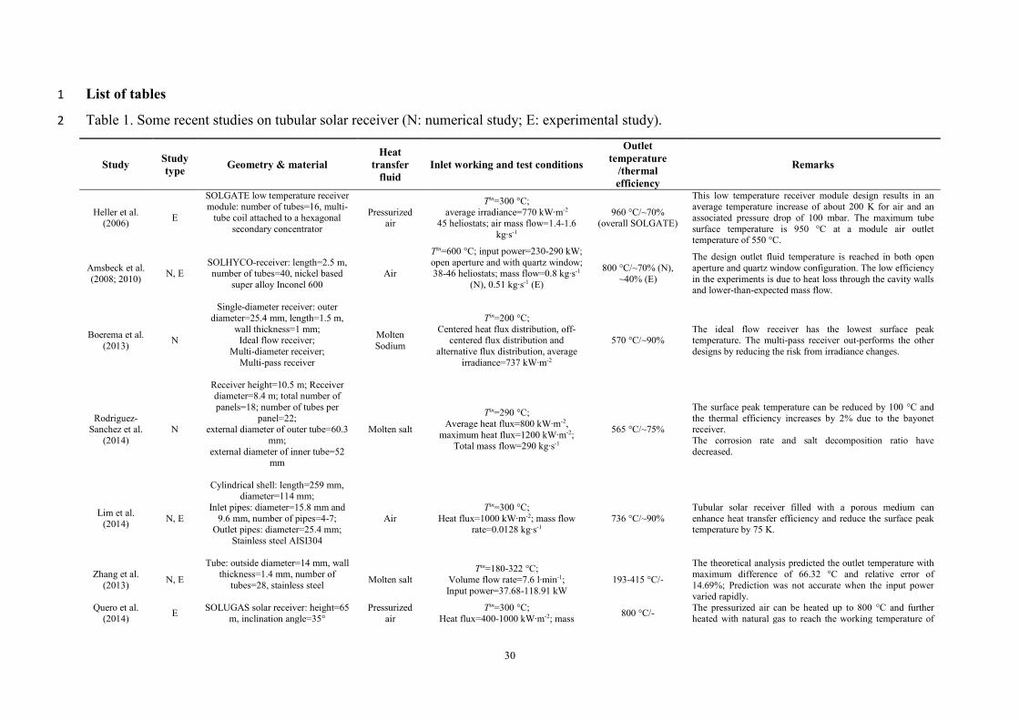
Depending on the geometrical configuration, the solar receivers can be classified into 12 different types, such as volumetric receiver, cavity receiver or particle receiver [6]. In 13 particular, tubular receivers are widely used in present commercial CSP projects because they 14 belong to a proven technology on concepts from heat exchanger which is relatively 15 inexpensive and durable [7, 8]. Some numerical or experimental studies on tubular solar 16 receivers in the recent literature are summarized in Table 1. Pressurized air or molten salt are 17 used as heat transfer fluid whereas the receiver is usually made of stainless steel or Inconel. 18

19

Table 1. Some recent studies on tubular solar receiver (N: numerical study; E: experimental study). 20

21

The lifetime of tubular solar receivers depends strongly on the thermal-mechanical stress on 22 the material which is in close relation with the peak temperature of the receiver wall [18]. 23 Based on the study of [19] on a pressurized-air solar receiver tube made of Alloy 617, the 24 lifetime is estimated about 30 years while operating 10 hours per day under peak temperature 25 of 1100 K. This temperature is also considered as the threshold temperature under which the 26 corresponding mechanical stress reaches the allowable design value that the material can 27 afford for normal operation. When peak wall temperature reaches 1250 K, the real mechanical 28 stress is 7.2 times the allowable design stress, resulting in a reduction of receiver lifetime by 29 a factor of 10 to 20. Moreover, a peak wall temperature of 1250 K instead of 1100 K increases 30 about 40% the thermal loss due to radiation, leading to more than 3% reduction in electricity 31 production. Therefore, how to decrease the peak temperature on the solar receiver wall is 32 becoming a serious concern. 33

The temperature distribution on the tubular solar receiver wall of a given geometry mainly 34 depends on the following factors. 35

• The material of the receiver: temperature and pressure-resisting materials with high 36 thermal conductivity are generally expected, but often require additional investment 37 cost and technology breakthrough on fabrication methods; 38

• The power and distribution of concentrated solar irradiation: uniform heat flux on the 39 receiver aperture is often assumed in theoretical analysis, but in reality very difficult to 40 achieve due to the large size of the receiver even with advanced aiming point strategy 41 [18, 20]. The actual heat flux distribution is generally non-uniform, either similar to a 42 Gaussian shape (e.g. Fig. 3) or to an alternative shape such as “table-top” distribution 43 [12]; 44

3

• The physical properties and the working conditions of heat transfer fluid: this is 1 usually determined by operational specifications of CSP plants; 2

• And finally the flow distribution of heat transfer fluid among the multiple parallel 3 tubes: this factor is relatively easier to be managed, but may play an important role on 4 reducing the peak temperature of the receiver wall. 5

Most of the studies in the literature aimed at uniformly distributing the heat transfer fluid 6 among parallel tubes under an assumed uniform solar irradiation. But when the solar 7 irradiation distribution on the receiver wall is in reality non-uniform, there must exist an 8 optimal fluid flow distribution so that the peak temperature of the receiver can be minimized. 9 Then the challenge is how to determine this optimal fluid flow distribution. Researches in this 10 area are relatively fewer and less recognized, with the exception of [12]. 11

In their work [12], an optimality criterion was proposed, suggesting that the peak temperature 12 can be largely reduced when the outlet fluid temperatures from parallel tubes are identical. 13 The theoretical fluid distribution for a single-layer tubular solar receiver could then be 14 determined based on a 1-D heat transfer model, using classic correlations for heat transfer and 15 fluid flow. Various improved receiver designs were also proposed, including multi-diameter 16 or multi-pass configurations. Nevertheless, the analytical solution obtained was more or less 17 approximate because of various simplifications made for the model, i.e. negligible axial heat 18 conduction, established turbulent flow, negligible entrance effect, etc. When dealing with 19 more complicated geometries (e.g. multiple layers of tubes rather than one layer) or transfer 20 mechanisms (e.g. significant non-uniformity in axial/longitudinal heat flux distribution), the 21 formulation of physical models and the solution could become cumbersome, sometimes even 22 impossible. 23

So emerges the idea that classic analytical approaches could benefit from modern 24 Computational Fluid Dynamics (CFD) simulation. The main objective of the present study is 25 to develop an original CFD-based evolutionary algorithm for the determination of the 26 optimal fluid flow distribution in a tubular solar receiver subjected to a non-uniform net heat 27 flux, so as to minimize the peak temperature on the receiver wall. 28

For this purpose, a real 3D pressurized-air solar receiver comprising of 45 parallel straight 29 tubes arranged in three layers will be used as a model for study. By comparison with simple 30 tube bundle design, this tube-in-matrix concept allows a better heat dissipation by conduction 31 inside the receiver [21, 22]. 32

We will firstly use “identical outlet fluid temperatures” proposed by [12] as the optimality 33 criterion (OC-I), appropriate for introducing the receiver geometry, for describing basic 34 principles of the evolutionary algorithm, and for illustrating the effectiveness of the algorithm 35 through an actual numerical example. The reduction of the peak temperature through the 36 optimization of fluid flow distribution will be presented and discussed. 37

Furthermore, a detailed analysis may reveal that such optimality criterion (identical outlet 38 fluid temperatures) does not necessarily mean minimum peak temperature on the receiver 39 wall. So a large section of this article is devoted to proposing a new evolutionary optimality 40 criterion for further reducing the peak temperature, taking the receiver geometry and the 41 physical properties of the material into account. The shapes of optimal fluid distribution, the 42 corresponding minimum peak temperatures for different filling materials and the effect of 43 thermal contact resistances will also be compared and discussed. 44

It should be emphasized that the present article is focused on the determination of the optimal 45 fluid flow distribution for a tubular solar receiver. The realization of such optimal distribution 46

4

by a simple and practical method is certainly an interesting subject with practical significance, 1 but is beyond the present paper. Some discussions may be found in the perspectives section of 2 the article, in connection to our earlier work on the design and optimization of fluid 3 distributors and collectors [23, 24]. 4

5

2. CFD-based Evolutionary Algorithm 6

In this section, a 3D multi-layer solar air receiver used as a model for study will be briefly 7 described. The basic principles of the evolutionary algorithm and the CFD simulation 8 parameters will be introduced as well. 9

10

2.1. Geometry of the tubular solar receiver: the tube-in-matrix concept 11

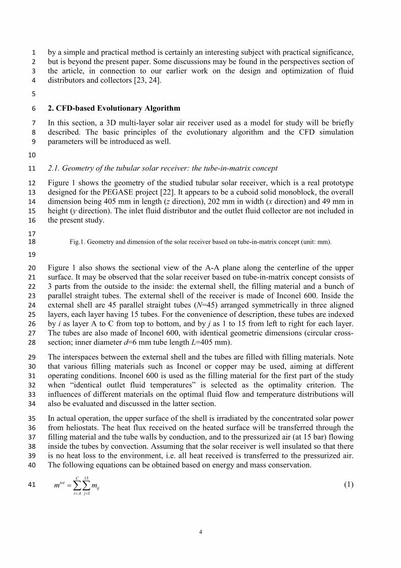
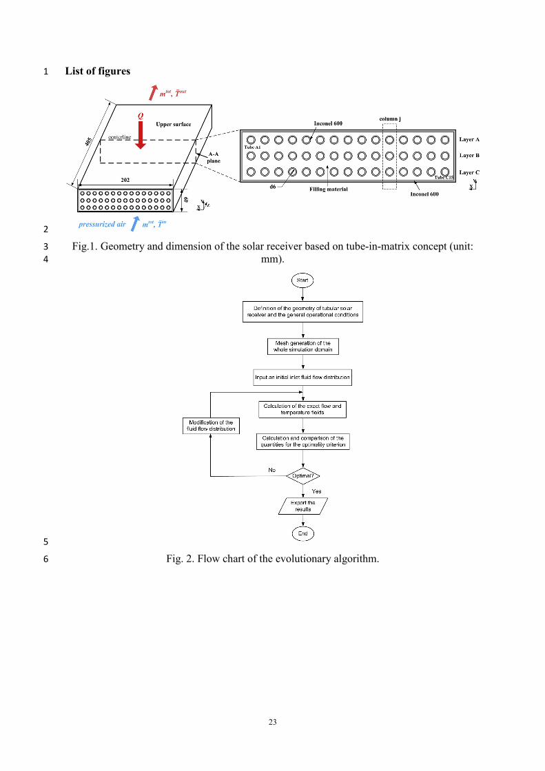
Figure 1 shows the geometry of the studied tubular solar receiver, which is a real prototype 12 designed for the PEGASE project [22]. It appears to be a cuboid solid monoblock, the overall 13 dimension being 405 mm in length (z direction), 202 mm in width (x direction) and 49 mm in 14 height (y direction). The inlet fluid distributor and the outlet fluid collector are not included in 15 the present study. 16

17 Fig.1. Geometry and dimension of the solar receiver based on tube-in-matrix concept (unit: mm). 18

19

Figure 1 also shows the sectional view of the A-A plane along the centerline of the upper 20 surface. It may be observed that the solar receiver based on tube-in-matrix concept consists of 21 3 parts from the outside to the inside: the external shell, the filling material and a bunch of 22 parallel straight tubes. The external shell of the receiver is made of Inconel 600. Inside the 23 external shell are 45 parallel straight tubes (N=45) arranged symmetrically in three aligned 24 layers, each layer having 15 tubes. For the convenience of description, these tubes are indexed 25 by i as layer A to C from top to bottom, and by j as 1 to 15 from left to right for each layer. 26 The tubes are also made of Inconel 600, with identical geometric dimensions (circular cross-27 section; inner diameter d=6 mm tube length L=405 mm). 28

The interspaces between the external shell and the tubes are filled with filling materials. Note 29 that various filling materials such as Inconel or copper may be used, aiming at different 30 operating conditions. Inconel 600 is used as the filling material for the first part of the study 31 when “identical outlet fluid temperatures” is selected as the optimality criterion. The 32 influences of different materials on the optimal fluid flow and temperature distributions will 33 also be evaluated and discussed in the latter section. 34

In actual operation, the upper surface of the shell is irradiated by the concentrated solar power 35 from heliostats. The heat flux received on the heated surface will be transferred through the 36 filling material and the tube walls by conduction, and to the pressurized air (at 15 bar) flowing 37 inside the tubes by convection. Assuming that the solar receiver is well insulated so that there 38 is no heat loss to the environment, i.e. all heat received is transferred to the pressurized air. 39 The following equations can be obtained based on energy and mass conservation. 40

15

1

Ctot

iji A j

m m= =

=∑∑

(1) 41

5

( )15 15

1 1

C Ctot out out in in

ij ij ij ij ij iji A j i A j

Q Q m Cp T Cp T= = = =

= = −∑∑ ∑∑ (2) 1

( )tot tot out out in inQ m Cp T Cp T= − (3)

2

where m is the fluid mass flow-rate, Q the heat transfer rate, Cp the specific heat of the fluid 3 and T the fluid temperature. The superscripts tot, in and out stand for total, inlet and outlet, 4 respectively. inT is the identical inlet fluid temperature ( in

ijin TT = ) whereas outT is the mass-5

averaged outlet fluid temperature calculated as: 6

tot

C

i j

outijij

out

m

TmT

∑∑= == 1

15

1

(4) 7

8

2.2. Basic principle for identical outlet fluid temperature distribution 9

The evolutionary algorithm is developed to determine the fluid flow distribution among 10 parallel tubes corresponding to the selected optimality criterion (OC-I: identical outlet fluid 11 temperatures): 12

out outijT T=

(5) 13

Since the outlet fluid temperature is directly linked to the mass flow-rate of fluid in the tube, 14 the optimality criterion could be reached by augmenting or reducing the flow-rate in the tubes 15 by comparing out

ijT and outT , while keeping the total mass flow-rate (mtot) constant. More 16

precisely, if the outlet fluid temperature of the tube ij is lower than the mean value, then the 17 flow-rate of this tube ijm should be reduced. Vice versa if out

ijT is higher than outT , ijm should 18

be increased to reach a lower outlet fluid temperature. The variation of different ijm according 19

to the difference between outijT and outT repeats iteratively until the optimality criterion Eq. (5) 20

is achieved. 21

Ideally, the increment or decrement of ijm from one optimization step to another should be as 22

small as possible. However, that will by far lengthen the calculation time thus it is not highly 23 efficient. Therefore, we introduce a variation rule as presented in Eq. (6). From t to t+1 step, 24 the variation of ijm is proportional to the difference between out

ijT and outT : 25

( ), , 1 , , , ,out out

ij t ij t ij t ij t ij t ij tm m m m T m Tγ+∆ = − = −

(6) 26

where γ is a relaxation factor always larger than zero to control the variation amplitude. 27 Following this rule, the total inlet mass flow-rate is approximately constant during the 28 optimization procedure, with the assumption that the variation of Cp is negligible (actually 29 <2.6%) within the range of tested temperature conditions 30

( ) ( ) ( )15 15 15

,, , , ,

1 1 1 ,

0totC C C

ij tout outij t ij t ij t ij t out out

i A j i A j i A j ij t

Q Qm m T m TCp T Cp T

γ γ= = = = = =

∆ = − = − ≈

∑∑ ∑∑ ∑∑ (7) 31

6

The initial value of γ is determined as the following: 1

, 1 , 0

, 1 , 1 , 0 , 0

max , , ; 1, 2,...,15 ij t ij tout out

ij t ij t ij t ij t

m mi A B C j

m T m Tγ =− =

=− =− = =

− = = = −

(8) 2

The initial fluid flow distribution as the beginning case (step t=0) could be arbitrary. Here a 3 uniform inlet fluid flow distribution is used. A conventional shape of flow distribution using 4 conventional rectangular or conic inlet/outlet headers is also introduced for comparison (step 5 t=-1), presenting a certain degree of non-uniformity (as shown in Fig. 5). 6

The degree of closeness between the optimized results and the optimality criterion is 7 quantified by the non-uniformity of outlet fluid temperatures (MFT) defined as follows: 8

215

T1

1MF1

out outCij

outi A j

T TN T= =

−= −

∑∑

(9) 9

The optimality criterion (OC-I) is considered to be achieved when values of MFT approach 0. 10 Meanwhile, the non-uniformity of fluid flow (MFf) frequently used [25, 26] can be written as: 11

215

f1

1MF1

Cij

i A j

m mN m= =

−= −

∑∑

(10) 12

where m is the mean mass flow-rate of all tubes: 13

N

mm

C

Ai jij∑∑

= ==

15

1 (11) 14

We also define Δpmax as the maximum pressure drop among parallel tubes. 15

16

2.3. Implementation of optimization procedure 17

The major steps of the CFD-based evolutionary algorithm are schematized in the following 18 flow chart (Fig. 2) and described in detail below. 19

（1） Input the initial data such as the size and initial geometry of the solar receiver, the 20 general operational conditions (the ambient temperature, operational pressure, net 21 heat flux distribution, etc.) and the physical properties of working fluid (fluid 22 nature, total inlet mass flow-rate, density, viscosity, etc.). 23

（2） Mesh generation of the whole simulation domain for both fluid and solid zones. 24

（3） Input an initial inlet fluid flow distribution among parallel tubes, e.g. a uniform 25 flow distribution as the beginning of evolutionary algorithm. 26

（4） Calculation of the exact flow and temperature fields by solving the Navier-Stokes 27 and heat transfer equations. 28

（5） Calculation of the quantities mentioned in the optimality criterion (the outlet fluid 29 temperature of each tube); modification of mass flow-rate distribution according to 30 the variation rule of Eq. (5). 31

7

（6） Recalculation of the exact flow and temperature fields to obtain the updated data. 1

（7） Check the stable tolerance of the evolutionary algorithm. If the tolerance is 2 satisfied, then the evolutionary procedure is considered to be converged. 3 Practically, the optimization process will be terminated when the value of MFT 4 becomes less than 0.001. If not so, the procedure goes back to Step 5 for 5 recurrence. 6

（8） Exportation of results, including the fluid flow distribution, the temperature field, 7 the peak temperature on the heated surface and the maximum pressure drop, etc. 8

9

Fig. 2. Flow chart of the evolutionary algorithm. 10

11

2.4. Calculation of flow and temperature fields by CFD method 12

An essential step of the evolutionary algorithm is the calculation of exact flow and 13 temperature fields. This generally involves solving Navier-Stokes equations and heat transfer 14 equations by CFD methods. For the fluid zone, the equation for conservation of mass or 15 continuity equation is: 16

( ) 0utρ ρ∂+∇⋅ =

∂

(12) 17

The momentum conservation equation is described by: 18

( ) ( ) ( )u uu p g Ftρ ρ ρ∂

+∇⋅ = −∇ +∇⋅ ∏ + +∂

(13) 19

where u is the velocity, p is the static pressure, gρ and F

are the gravitational body force 20 and external body forces, ∏ is the stress tensor given by: 21

( )T 23

u u uIµ ∏ = ∇ +∇ − ∇⋅

(14) 22

where μ is the molecular viscosity, I is the unit tensor. 23

The energy equation is: 24

( ) ( )( ) ( ) : HE u E p T u Qtρ ρ λ ρ∂

+∇⋅ + = ∇ ⋅ ∇ +∏ ∇ +∂

(15) 25

where E is the internal energy, λ is the thermal conductivity, and QH includes the heat of 26 chemical reaction, radiation and any other volumetric heat sources. To predict turbulent flow 27 pattern, additional turbulence models should be employed. 28

For the solid zone, the energy transport equation is: 29

( ) hTC T St

ρ λ∂= ∇⋅ ∇ +

∂ (16) 30

where C is the specific heat and hS is the heat sources within the solid. 31

32

8

2.5. Numerical parameters for CFD simulation 1

Meshes were generated using software ICEM (version 12.1) to build up the geometry model 2 of the studied solar receiver. Note that half of the real object was adopted for the purpose of 3 lessening the computational burden because of the symmetric feature for both the simulation 4 domain and the net heat flux distribution. The grid used in this study had 3 680 940 elements 5 in total, with 1 421 550 structured hexahedral elements for fluid zone and 2 259 390 6 unstructured hexahedral elements for solid zone. Relatively more mesh elements were used 7 for the fluid zone (38.6% grid for 12.9% volume) since the physical properties of pressurized 8 air are strongly temperature dependent. A grid independence study was conducted to 9 guarantee that the current mesh density used was appropriate and sufficient regarding both 10 accuracy and calculation time. 11

The working fluid used was pressurized air at 15 bar while the solar receiver manufacturing 12 material was Inconel 600. The physical properties of fluid and solid were considered as 13 temperature dependent, using the polynomial fitting correlations listed in Table 2. It should be 14 noted that the expansion properties of solid material were ignored in our study. 15

16

Table 2. Physical properties of fluid and solid used for simulations [27]. 17

18

In this study, 3D fluid flow simulations were performed under steady state with heat transfer, 19 using a commercial code FLUENT (version 12.1.4). The gravity effect was also considered. 20 Standard k-ε model was used to simulate the potential turbulent flow. For the pressure-21 velocity coupling, COUPLED method was used. For discretization, standard method was 22 chosen for pressure and first-order upwind differentiation for momentum. 23

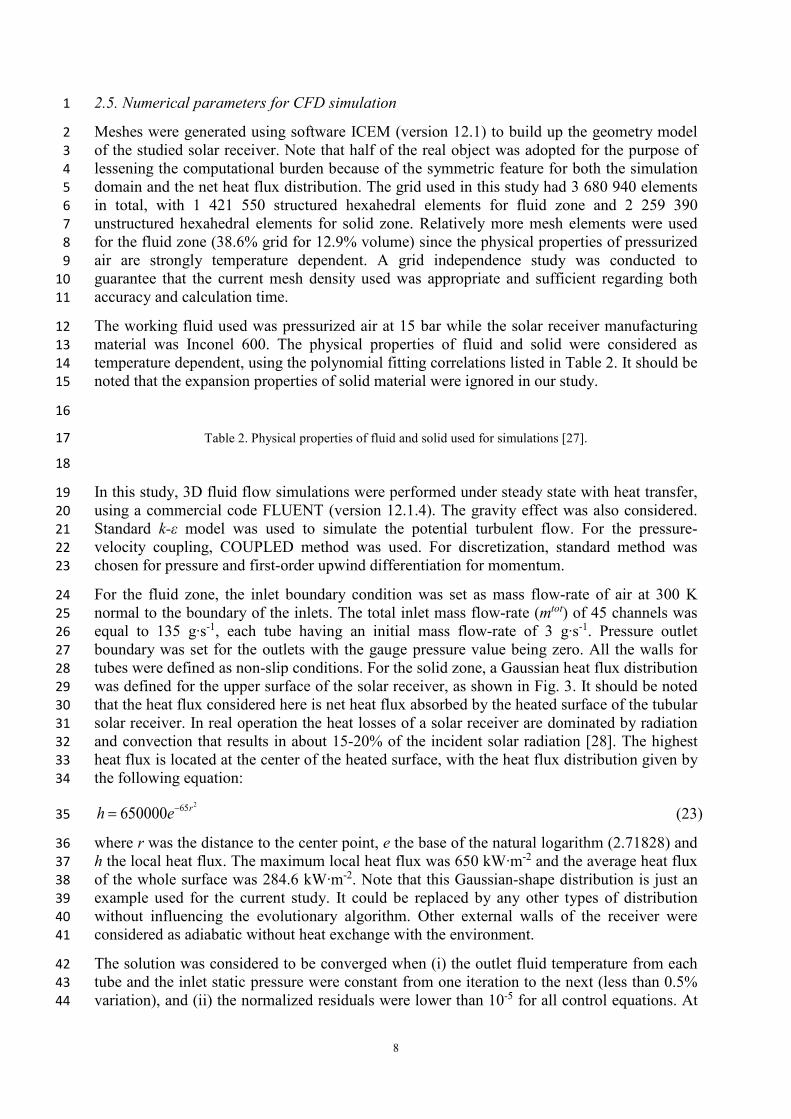
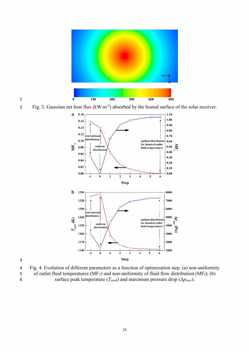
For the fluid zone, the inlet boundary condition was set as mass flow-rate of air at 300 K 24 normal to the boundary of the inlets. The total inlet mass flow-rate (mtot) of 45 channels was 25 equal to 135 g∙s-1, each tube having an initial mass flow-rate of 3 g∙s-1. Pressure outlet 26 boundary was set for the outlets with the gauge pressure value being zero. All the walls for 27 tubes were defined as non-slip conditions. For the solid zone, a Gaussian heat flux distribution 28 was defined for the upper surface of the solar receiver, as shown in Fig. 3. It should be noted 29 that the heat flux considered here is net heat flux absorbed by the heated surface of the tubular 30 solar receiver. In real operation the heat losses of a solar receiver are dominated by radiation 31 and convection that results in about 15-20% of the incident solar radiation [28]. The highest 32 heat flux is located at the center of the heated surface, with the heat flux distribution given by 33 the following equation: 34

265650000 rh e−= (23) 35

where r was the distance to the center point, e the base of the natural logarithm (2.71828) and 36 h the local heat flux. The maximum local heat flux was 650 kW∙m-2 and the average heat flux 37 of the whole surface was 284.6 kW∙m-2. Note that this Gaussian-shape distribution is just an 38 example used for the current study. It could be replaced by any other types of distribution 39 without influencing the evolutionary algorithm. Other external walls of the receiver were 40 considered as adiabatic without heat exchange with the environment. 41

The solution was considered to be converged when (i) the outlet fluid temperature from each 42 tube and the inlet static pressure were constant from one iteration to the next (less than 0.5% 43 variation), and (ii) the normalized residuals were lower than 10-5 for all control equations. At 44

9

each optimization step, MATLAB was used to take the computed flow and temperature fields 1 data from FLUENT, to perform calculations of the flow-rate change for each tube according 2 to Eq. (6) and to pass the data required to FLUENT to recalculate the updated flow and 3 temperature fields. 4

5

Fig. 3. Gaussian net heat flux (kW∙m-2) absorbed by the heated surface of the solar receiver. 6

7

3. Results and discussion 8

3.1. Effectiveness of the evolutionary algorithm 9

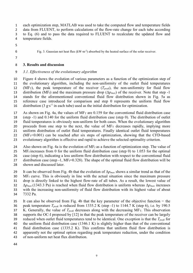
Figure 4 shows the evolution of various parameters as a function of the optimization step of 10 the evolutionary algorithm, including the non-uniformity of the outlet fluid temperatures 11 (MFT), the peak temperature of the receiver (Tpeak), the non-uniformity for fluid flow 12 distribution (MFf) and the maximum pressure drop (Δpmax) of the receiver. Note that step -1 13 stands for the aforementioned conventional fluid flow distribution shown in Fig. 5a as 14 reference case introduced for comparison and step 0 represents the uniform fluid flow 15 distribution (3 g∙s-1 in each tube) used as the initial distribution for optimization. 16

As shown on Fig. 4a, the values of MFT are 0.159 for the conventional fluid distribution case 17 (step -1) and 0.140 for the uniform fluid distribution case (step 0). The distribution of outlet 18 fluid temperatures is obviously non-uniform for both cases. When the evolutionary algorithm 19 proceeds from one step to the next, the value of MFT decreases rapidly, implying more 20 uniform distribution of outlet fluid temperatures. Finally identical outlet fluid temperatures 21 (MFT<0.001) can be reached after six steps of optimization, showing that the CFD-based 22 evolutionary algorithm is effective and rapid to achieve the selected optimality criterion. 23

Also shown on Fig. 4a is the evolution of MFf as a function of optimization step. The value of 24 MFf increases from 0 for the uniform fluid distribution case (step 0) to 1.053 for the optimal 25 case (step 6), indicating a less uniform flow distribution with respect to the conventional fluid 26 distribution case (step -1, MFf=0.328). The shape of the optimal fluid flow distribution will be 27 shown and discussed later. 28

It can be observed from Fig. 4b that the evolution of Δpmax shows a similar trend as that of the 29 MFf curve. This is obviously in line with the actual situation since the maximum pressure 30 drop is directly linked to the highest flow-rate of all tubes. As a result, the lowest value of 31 Δpmax (1343.3 Pa) is reached when fluid flow distribution is uniform whereas Δpmax increases 32 with the increasing non-uniformity of fluid flow distribution with its highest value of about 33 7332 Pa. 34

It can also be observed from Fig. 4b that the key parameter of the objective function ̶ the 35 peak temperature Tpeak is reduced from 1335.2 K (step -1) to 1144.7 K (step 6), i.e. by 190.5 36 K. Generally, the value of Tpeak decreases along with the decreasing MFT. This observation 37 supports the OC-I proposed by [12] in that the peak temperature of the receiver can be largely 38 reduced when outlet fluid temperatures tend to be identical. One exception is that the Tpeak for 39 the uniform fluid distribution case (1346.1 K) is slightly higher than that of the conventional 40 fluid distribution case (1335.2 K). This confirms that uniform fluid flow distribution is 41 apparently not the optimal option regarding peak temperature reduction, under the condition 42 of non-uniform net heat flux distribution. 43

44

10

Fig. 4. Evolution of different parameters as a function of optimization step. (a) non-uniformity of outlet fluid 1 temperatures (MFT) and non-uniformity of fluid flow distribution (MFf); (b) surface peak temperature (Tpeak) and 2

maximum pressure drop (Δpmax). 3

4

3.2. Comparison of three cases 5

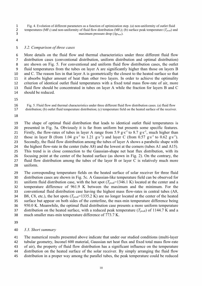
More details on the fluid flow and thermal characteristics under three different fluid flow 6 distribution cases (conventional distribution, uniform distribution and optimal distribution) 7 are shown on Fig. 5. For conventional and uniform fluid flow distribution cases, the outlet 8 fluid temperatures from the tubes on layer A are significantly higher than those on layers B 9 and C. The reason lies in that layer A is geometrically the closest to the heated surface so that 10 it absorbs higher amount of heat than other two layers. In order to achieve the optimality 11 criterion of identical outlet fluid temperatures with a fixed total mass flow-rate of air, more 12 fluid flow should be concentrated in tubes on layer A while the fraction for layers B and C 13 should be reduced. 14

15

Fig. 5. Fluid flow and thermal characteristics under three different fluid flow distribution cases. (a) fluid flow 16 distribution; (b) outlet fluid temperature distribution; (c) temperature field on the heated surface of the receiver. 17

18

The shape of optimal fluid distribution that leads to identical outlet fluid temperatures is 19 presented in Fig. 5a. Obviously it is far from uniform but presents some specific features. 20 Firstly, the flow-rates of tubes in layer A range from 5.9 g∙s-1 to 8.7 g∙s-1, much higher than 21 those in layer B (from 1.04 g∙s-1 to 1.21 g∙s-1) and layer C (from 0.57 g∙s-1 to 0.62 g∙s-1). 22 Secondly, the fluid flow distribution among the tubes of layer A shows a parabolic shape with 23 the highest flow-rate in the center (tube A8) and the lowest at the corners (tubes A1 and A15). 24 This trend is in close connection to the Gaussian-shape net heat flux distribution, with its 25 focusing point at the center of the heated surface (as shown in Fig. 2). On the contrary, the 26 fluid flow distribution among the tubes of the layer B or layer C is relatively much more 27 uniform. 28

The corresponding temperature fields on the heated surface of solar receiver for three fluid 29 distribution cases are shown in Fig. 5c. A Gaussian-like temperature field can be observed for 30 uniform fluid distribution case, with the hot spot (Tpeak=1346.1 K) located at the center and a 31 temperature difference of 961.9 K between the maximum and the minimum. For the 32 conventional fluid distribution case having the highest mass flow-rates in central tubes (A8, 33 B8, C8, etc.), the hot spots (Tpeak=1335.2 K) are no longer located at the center of the heated 34 surface but appear on both sides of the centerline, the max-min temperature difference being 35 950.0 K. Meanwhile, the optimal fluid distribution case presents a more uniform temperature 36 distribution on the heated surface, with a reduced peak temperature (Tpeak) of 1144.7 K and a 37 much smaller max-min temperature difference of 773.7 K. 38

39

3.3. Short summary 40

The numerical results presented above indicate that under our studied conditions (multi-layer 41 tubular geometry, Inconel 600 material, Gaussian net heat flux and fixed total mass flow-rate 42 of air), the property of fluid flow distribution has a significant influence on the temperature 43 distribution on the heated surface of the solar receiver. By simply arranging the fluid flow 44 distribution in a proper way among the parallel tubes, the peak temperature could be reduced 45

11

by about 200 K. This optimal fluid flow distribution can be easily determined by our CFD-1 based evolutionary algorithm, using identical outlet fluid temperatures as the optimality 2 criterion. 3

One may be satisfied with these encouraging results but another question may arise: is the 4 optimality criterion of identical outlet fluid temperatures equivalent to the minimum peak 5 temperature of the heated surface? Note that it is the peak temperature rather than the 6 uniformity of outlet fluid temperature that is the main issue of concern in relation to the 7 lifetime of solar receivers. The answer is perhaps not: the peak temperature is largely reduced 8 but there is no evidence that it achieves the minimum. Then one may ask: can the peak 9 temperature be further reduced by acting on the fluid flow distribution? If yes, could this 10 optimal fluid distribution be determined by the proposed evolutionary algorithm? Furthermore, 11 what will be the effects of fluid flow distribution on the peak temperature reduction when 12 different filling materials are used for the solar receiver? The following section aims at 13 answering these questions by proposing a new evolutionary optimality criterion (OC-II) for 14 the CFD-based evolutionary algorithm. 15

16

4. A new optimality criterion for peak temperature minimization 17

By carefully examining the temperature field of the heated surface for the optimal fluid 18 distribution case (Fig. 5c), one may observe that it still shows a Gaussian-like shape with the 19 hot-spot located at the center of the heated surface. The temperature distribution is not 20 uniform along with the x direction of the receiver, i.e. the isothermal lines are not 21 perpendicular to the fluid flow direction. It seems that the peak temperature can be further 22 reduced by concentrating more fluid flow into the central tubes (e.g. A7, A8, A9) while 23 decreasing the flow-rates in tubes on the edge (e.g. A1, A15). In brief, the optimality criterion 24 of identical outlet fluid temperatures (OC-I) does not necessarily lead to the minimum peak 25 temperature. If one aims at minimizing the peak temperature, the optimality criterion used 26 should be modified and the corresponding optimal fluid flow distribution will be differed 27 from that shown in Fig. 5a. 28

The main motivation of this section is thus to propose a new evolutionary optimality criterion 29 (OC-II) that leads to minimum peak temperature of the heated surface. The corresponding 30 optimal fluid flow distribution can still be determined using the developed CFD-based 31 evolutionary algorithm. 32

33

4.1. Description of the new optimality criterion 34

The basic idea is to adjust the fluid flow distribution among the parallel tubes so that 35 isothermal lines on the heated surface are perpendicular to the fluid flow direction. Due to the 36 Gaussian-shape net heat flux distribution, the peak temperature is always located on the 37 centerline of the heated surface. As a result, identical temperatures on the centerline 38 perpendicular to the fluid flow direction may be proposed as the new optimality criterion 39 (OC-II). 40

Once the new optimality criterion is proposed, the next step is to establish the variation rule 41 for the mass flow-rate in each tube to realize this OC-II. This calls for a detailed analysis on 42 coupled heat transfer and fluid flow to reveal the relationship between the flow-rate change in 43 each channel and the temperature variation on the centerline. To do that, we reduce the 3D 44 multi-layer tubular solar receiver problem into 2D, by selecting the middle cross section (A-A 45

12

plane shown in Fig. 1) as the study plane. Note that at steady state, the mass flow-rate of fluid 1 at different cross-sections (i.e. tube inlet, middle cross-section, tube outlet) of each tube is 2 constant. 3

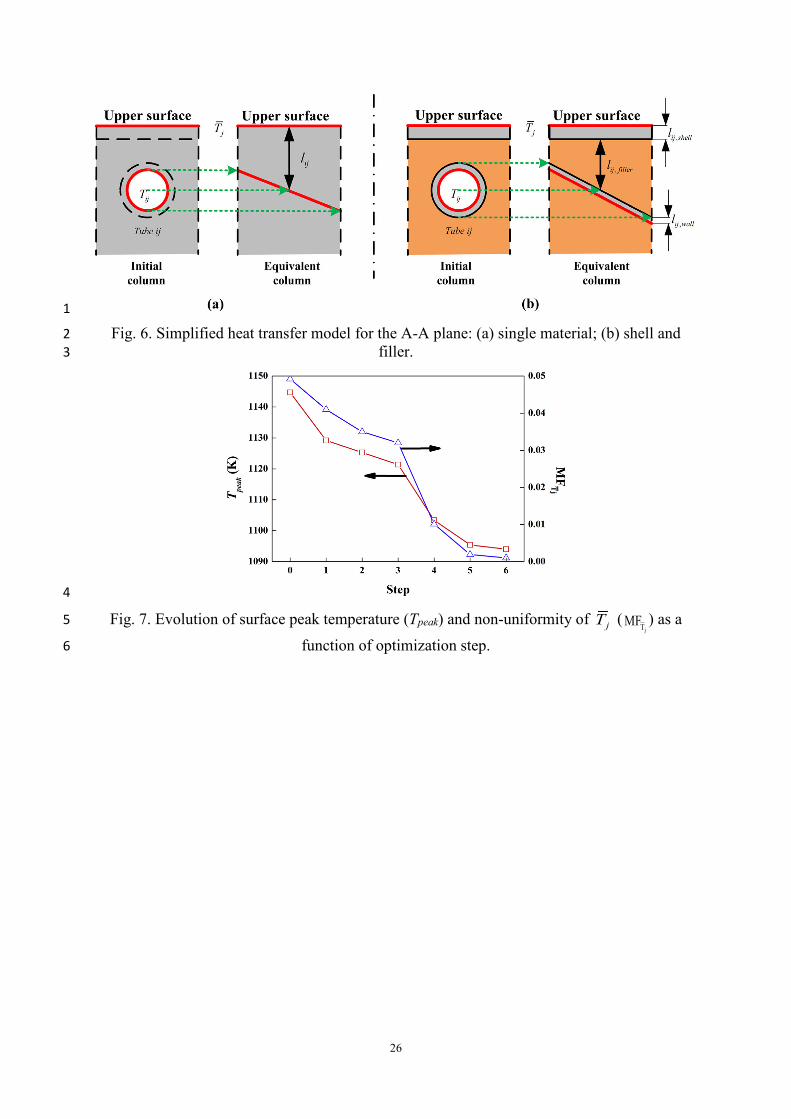
The schematic view of the middle cross-section (A-A plane) is shown in Fig. 1. Recall that 4 the tubes are indexed as ij (i represents layer from A to C and j represents the index of column 5 from 1 to 15). The middle cross-section is divided into 15 columns. In each column, there are 6 three tubes of different layers (e.g. tubes A1, B1, C1 in column 1). Figure 6 shows a 7 simplified heat conduction model from the upper line of each column to the inner wall of one 8 tube. We note the mean temperature on the upper line of column j as jT and the average 9

temperature of inner wall of tube ij as ijT . By using an equivalent distance between the upper 10

line and the inner tube wall (as shown in Fig. 6a), the conduction heat flux for the single solid 11 material condition (Inconel 600) can be written as follows: 12

j ijij

ij

ij

T Tlλ

−Φ = (24) 13

where ijλ is the average thermal conductivity of solid material: 14

( )2

j ijT Tij TTλ λ +

==

(25) 15

16

Fig. 6. Simplified heat transfer model for the A-A plane: (a) single material; (b) shell and filler. 17

18

When different filling materials other than Inconel 600 are used (Fig. 6b), we assume that the 19 solar receiver is perfectly fabricated so that thermal contact resistances at material interfaces 20 are negligible. Then Eq. (24) could be written as: 21

, , ,

, , ,

j ijij

ij shell ij filler ij wall

ij shell ij filler ij wall

T Tl l lλ λ λ

−Φ =

+ +

(26) 22

In order to achieve identical temperatures on the centerline (upper line of the middle cross-23 section), the mass flow-rate in each tube ijm will be modulated by comparing ijΦ and the 24

average Φ of tubes. More precisely, if ijΦ is higher than Φ , the mass flow-rate in tube ij 25

should be increased to further enhance the heat transfer. Vice versa if ijΦ is smaller than Φ , 26

the flow-rate in the tube ij should be reduced because of the poor heat transfer potential. 27

To realize the new optimality criterion step-by-step by the CFD-based evolutionary algorithm, 28 a variation rule is introduced as follows: 29

( ), , 1 ,ij t ij t ij t ijm m m γ+∆ = − = Φ −Φ

(27) 30

where γ is the aforementioned relaxation factor in Eq. (7). It should be noted that during the 31 optimization steps, the mass flow-rate in some tubes may approach zero. Therefore the 32 average Φ is calculated as: 33

13

( )

15

1 0

C

iji A j

ijfor mN

= =

ΦΦ = >

′

∑∑

(28) 1

where N’ is the number of tubes whose flow-rates are not equal to zero. 2

The shape of optimal fluid distribution obtained for identical outlet fluid temperatures (Fig. 5a) 3 is used as the beginning case (step 0) this time. The implementation of the CFD-based 4 evolutionary algorithm is similar as that shown in Fig. 2 and explained in section 2.3. The 5 main distinction is the use of new optimality criterion of identical temperatures on the 6 centerline so that the termination condition of the algorithm is defined as: 7

( )1,2,...,15jT T j= = (29) 8

where T is the mean temperature of all 15 jT . 9

15

1

15

jj

TT ==

∑

(30) 10

Practically, we consider that the new optimality criterion is achieved whenjTMF is less than 11

0.001, where jTMF is the non-uniformity of jT calculated as: 12

j

215

T1

1MF14

j

j

T T

T=

− =

∑

(31) 13

14

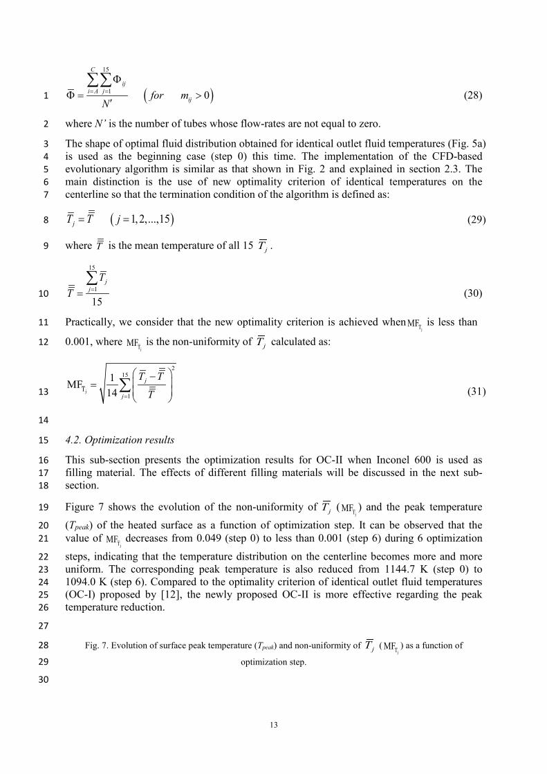
4.2. Optimization results 15

This sub-section presents the optimization results for OC-II when Inconel 600 is used as 16 filling material. The effects of different filling materials will be discussed in the next sub-17 section. 18

Figure 7 shows the evolution of the non-uniformity of jT (jTMF ) and the peak temperature 19

(Tpeak) of the heated surface as a function of optimization step. It can be observed that the 20 value of

jTMF decreases from 0.049 (step 0) to less than 0.001 (step 6) during 6 optimization 21

steps, indicating that the temperature distribution on the centerline becomes more and more 22 uniform. The corresponding peak temperature is also reduced from 1144.7 K (step 0) to 23 1094.0 K (step 6). Compared to the optimality criterion of identical outlet fluid temperatures 24 (OC-I) proposed by [12], the newly proposed OC-II is more effective regarding the peak 25 temperature reduction. 26

27

Fig. 7. Evolution of surface peak temperature (Tpeak) and non-uniformity of jT (jTMF ) as a function of 28

optimization step. 29

30

14

The optimal fluid flow distribution corresponding to the OC-II is shown in the first row of Fig. 1 8. It can be observed that the vast majority of mass flow (97%) is concentrated in tubes of 2 layer A, showing a parabolic shape with the highest value (11.9 g∙m-1) in the middle (tube A8) 3 and the lowest (4.81 g∙m-1) at the corners (tubes A1 and A15). Several tubes in layer B (B5-4 B11) have a small proportion of mass flow (3%) ranging from 0.2 g∙m-1 to 0.88 g∙m-1, while 5 tubes in layer C are totally empty. By comparing Fig. 8a and Fig. 5a, one may find that 6 increasing the mass flow-rate proportion in tubes closer to the heat source could further 7 reduce the peak temperature of the heated surface. 8

Figure 8a also shows the corresponding temperature field on the heated surface. It can be 9 observed that the isothermal lines on the heated surface are by and large perpendicular to the 10 direction of fluid flow so that the peak temperature of the heated surface may be considered to 11 be minimized. 12

13

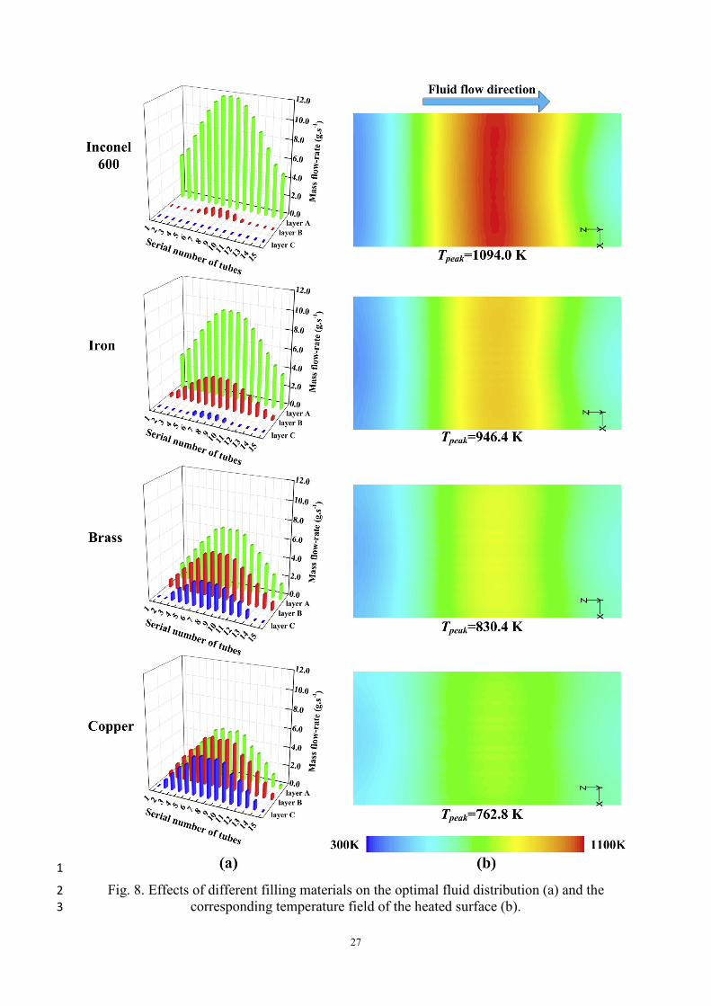
Fig. 8. Effects of different filling materials on the optimal fluid distribution (a) and the corresponding 14 temperature field of the heated surface (b) 15

16

4.3. Effect of different filling materials 17

From the viewpoint of heat transfer, Inconel 600 may not be that favorable as filling material 18 due to its relatively low thermal conductivity (about 20 W∙m-1∙K-1). In order to evaluate the 19 effectiveness of the OC-II and the influence of optimal fluid distribution on peak temperature 20 reduction under different filling material conditions, three filling materials (iron, brass and 21 copper) with higher thermal conductivities are introduced for comparison. The physical 22 proprieties of the studied materials within the tested temperature range used in the CFD 23 simulations are listed in Table 3. 24

25

Table 3. Physical proprieties of different filling materials within the tested temperature (K) range [27, 29]. 26

27

Figure 8 shows the shape of optimal fluid distribution, the corresponding temperature field of 28 the heated surface and the minimum peak temperature for different filling materials. For every 29 filling material, the isothermal lines are all perpendicular to the fluid flow direction, without 30 obvious “hot spots” on the heated surface. This confirms the fact that the new optimality 31 criterion is applicable to various filling materials with different thermal conductivities. 32

It can also be observed from Fig. 8a that the shape of optimal fluid distribution is greatly 33 differed from one filling material to another. The higher the thermal conductivity of filling 34 material, the higher proportion of mass flow will be shared by the layers far from the heated 35 surface. When copper is used as filling material, the proportion of mass flow-rate for layer A, 36 B and C is 35.5%, 36.9% and 27.6%, respectively. Let us notice that for Inconel 600, these 37 values are 97.0% (layer A), 3.0% (layer B) and 0.0% (layer C). This trend is in line with the 38 smaller thermal resistance for heat conduction when high thermal conductivity filling 39 materials are used. Higher mass flow-rates are thus necessary for tubes in layer B or C to 40 evacuate more heat flux transferred from the heated surface. 41

The obtained results also indicate that when Inconel 600 is used as filling material, multiple-42 layer design may not be necessary since tubes in layers B and C are almost not used. By 43 optimizing the fluid flow distribution under the new optimality criterion, one layer of parallel 44 tubes is sufficient for saving the materials. On the contrary when brass or copper is used as 45

15

filling material, all three layers are useful. One or more additional layers could also be 1 arranged for the receiver design with the purpose of reducing the total pressure drop with the 2 same load. 3

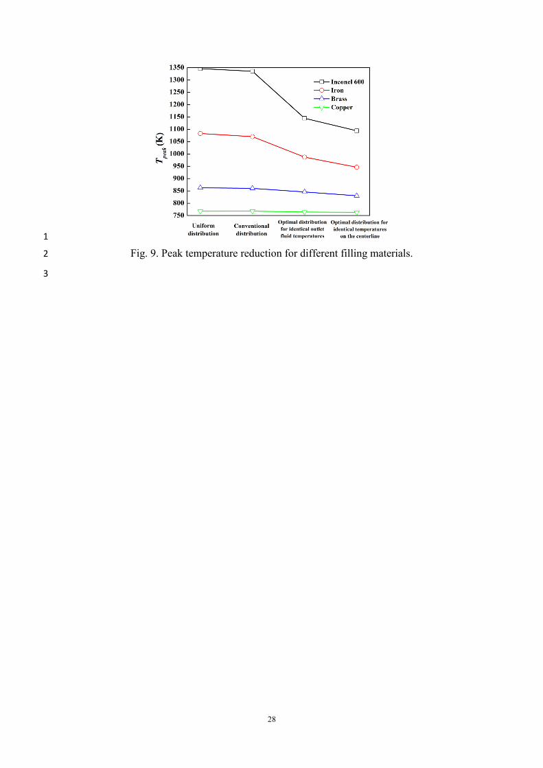
Figure 9 presents the calculated results of peak temperature (Tpeak) for four filling materials, 4 under different fluid flow distribution conditions, i.e. conventional distribution, uniform 5 distribution, optimal distribution for OC-I and optimal distribution for OC-II. For every filling 6 material, the peak temperature is the lowest when fluid flow distribution is optimized for 7 identical temperatures on the centerline, indicating the effectiveness of the new optimality 8 criterion and the evolutionary algorithm. 9

10

Fig. 9. Peak temperature reduction for different filling materials. 11

12

It can also be observed from Fig. 9 that the use of filling material with high thermal 13 conductivity could significant reduce the peak temperature than that with low thermal 14 conductivity. The minimum peak temperature decreases from 1094 K for Inconel 600, to 15 946.4 K for iron, to 830.4 K for brass and just to 762.8 K for copper. This implies that filling 16 material with high thermal conductivity (e.g. copper) is much more favorable in practical use 17 regarding peak temperature reduction, but usually requires higher cost. In contrast for simpler 18 assembly using one single refractory alloy with low thermal conductivity (e.g. Inconel 600), 19 the peak temperature of the receiver could be minimized from 1349 K to 1094 K (below the 20 threshold value of 1100 K) through simply optimizing the fluid flow distribution. In this sense, 21 the efforts of fluid flow distribution optimization seem to be worthwhile regarding lower 22 material cost and easier fabrication. 23

24

4.4. Effect of thermal contact resistance 25

In the above analysis, we assumed perfect contacts between different materials in the tubes-26 in-matrix concept so that the thermal contact resistances at materials’ interfaces were 27 neglected. However, due to the fabrication process, thermal contact resistances may not be 28 negligible especially for materials with relatively high thermal conductivity. In this section, 29 possible effects of thermal contact resistances on the peak temperature of the receiver and on 30 the optimal shape of flow distribution will be tested and discussed by some additional cases, 31 using copper as the filling material. 32

In fact, the thermal contact resistances could be easily taken into account in our CFD-based 33 evolutionary algorithm. To do that, additional values of thermal resistance are assigned as 34 boundary condition for interfaces (between the shell and the filling material, and between the 35 filling material and the Inconel tubes) in CFD simulations. For the evolutionary algorithm, an 36 extra term (1/hc) should be added in Eq. (26) for representing the global thermal contact 37 resistance: 38

, , ,

, , ,

1j ij

ijij shell ij filler ij wall

ij shell ij filler ij wall c

T Tl l l

hλ λ λ

−Φ =

+ + +

(35) 39

where ch is the global thermal contact conductance and its reciprocal is the global thermal 40 contact resistance. 41

16

The thermal contact resistance depends on many factors such as the roughness of contact 1 surfaces, the properties of the contacting materials (i.e. hardness, thermal conductivity, etc.), 2 and the operational conditions (i.e. pressure, temperature, etc.). Therefore, the exact values 3 vary widely in different cases and are difficult to be determined. In this study we used the 4 correlation proposed by [30] to make a rough estimation of the order of magnitude: 5

0.950.2574200c s a

Ph RH

λ − =

(36) 6

where P is the contact pressure, H is the surface micro hardness, Ra is the combined average 7 roughness and sλ is the harmonic mean thermal conductivity given by [30]: 8

1 2

1 2

2s

λ λλλ λ

=+

(37) 9

where 1λ and 2λ are the thermal conductivities of two contacted materials (Inconel and 10 copper). Note that under ideal condition when contacted surfaces are perfectly fabricated and 11 very smooth, the value of Ra reaches zero, implying zero thermal contact resistances. 12

Using proper values for different parameters, the reasonable value of thermal contact 13 resistance between Inconel and copper is estimated in the order of magnitude of 10-5 m2∙K∙W-14 1. Of course this value augments when surface roughness increases or fabrication defects 15 occur. As a result, two values, 1/hc=1×10-5 m2∙K∙W-1 and 1/hc=1×10-4 m2∙K∙W-1, have been 16 tested to represent low and high thermal contact resistance. 17

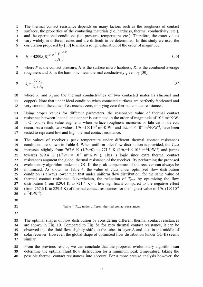
The values of receiver’s peak temperature under different thermal contact resistances 18 conditions are shown in Table 4. When uniform inlet flow distribution is provided, the Tpeak 19 increases slightly from 767.6 K (1/hc=0) to 771.3 K (1/hc=1×10-5 m2∙K∙W-1) and jumps 20 towards 829.4 K (1/hc=1 × 10-4 m2∙K∙W-1). This is logic since extra thermal contact 21 resistances augment the global thermal resistance of the receiver. By performing the proposed 22 evolutionary algorithm under the OC-II, the peak temperature of the receiver can always be 23 minimized. As shown in Table 4, the value of Tpeak under optimized flow distribution 24 condition is always lower than that under uniform flow distribution, for the same value of 25 thermal contact resistance. Nevertheless, the reduction of Tpeak by optimizing the flow 26 distribution (from 829.4 K to 821.4 K) is less significant compared to the negative effect 27 (from 767.6 K to 829.4 K) of thermal contact resistances for the highest value of 1/hc (1×10-4 28 m2∙K∙W-1). 29

30

Table 4. Tpeak under different thermal contact resistances 31

32

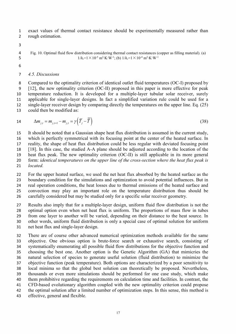
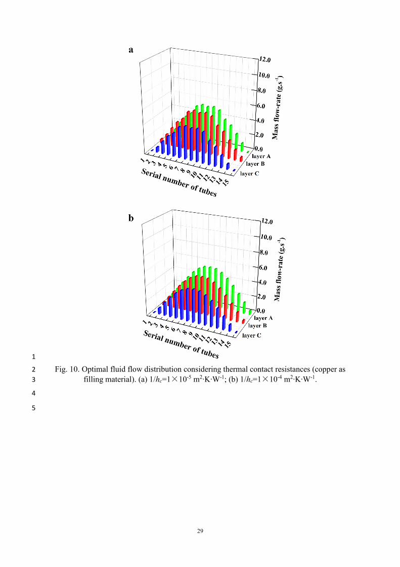
The optimal shapes of flow distribution by considering different thermal contact resistances 33 are shown in Fig. 10. Compared to Fig. 8a for zero thermal contact resistance, it can be 34 observed that the fluid flow slightly shifts to the tubes in layer A and also in the middle of 35 solar receiver. However, the global shape of optimized flow distribution (under OC-II) seems 36 similar. 37

From the previous results, we can conclude that the proposed evolutionary algorithm can 38 determine the optimal fluid flow distribution for a minimum peak temperature, taking the 39 possible thermal contact resistances into account. For a more precise analysis however, the 40

17

exact values of thermal contact resistance should be experimentally measured rather than 1 rough estimation. 2

3

Fig. 10. Optimal fluid flow distribution considering thermal contact resistances (copper as filling material). (a) 4 1/hc=1×10-5 m2∙K∙W-1; (b) 1/hc=1×10-4 m2∙K∙W-1 5

6

4.5. Discussions 7

Compared to the optimality criterion of identical outlet fluid temperatures (OC-I) proposed by 8 [12], the new optimality criterion (OC-II) proposed in this paper is more effective for peak 9 temperature reduction. It is developed for a multiple-layer tubular solar receiver, surely 10 applicable for single-layer designs. In fact a simplified variation rule could be used for a 11 single-layer receiver design by comparing directly the temperatures on the upper line. Eq. (25) 12 could then be modified as: 13

( ), , 1 ,j t j t j t jm m m T Tγ+∆ = − = −

(38) 14

It should be noted that a Gaussian shape heat flux distribution is assumed in the current study, 15 which is perfectly symmetrical with its focusing point at the center of the heated surface. In 16 reality, the shape of heat flux distribution could be less regular with deviated focusing point 17 [18]. In this case, the studied A-A plane should be adjusted according to the location of the 18 heat flux peak. The new optimality criterion (OC-II) is still applicable in its more general 19 form: identical temperatures on the upper line of the cross-section where the heat flux peak is 20 located. 21

For the upper heated surface, we used the net heat flux absorbed by the heated surface as the 22 boundary condition for the simulations and optimization to avoid potential influences. But in 23 real operation conditions, the heat losses due to thermal emissions of the heated surface and 24 convection may play an important role on the temperature distribution thus should be 25 carefully considered but may be studied only for a specific solar receiver geometry. 26

Results also imply that for a multiple-layer design, uniform fluid flow distribution is not the 27 optimal option even when net heat flux is uniform. The proportions of mass flow in tubes 28 from one layer to another will be varied, depending on their distance to the heat source. In 29 other words, uniform fluid distribution is only a special case of optimal solution for uniform 30 net heat flux and single-layer design. 31

There are of course other advanced numerical optimization methods available for the same 32 objective. One obvious option is brute-force search or exhaustive search, consisting of 33 systematically enumerating all possible fluid flow distributions for the objective function and 34 choosing the best one. Another option is the Genetic Algorithm (GA) that mimicries the 35 natural selection of species to generate useful solution (fluid distribution) to minimize the 36 objective function (peak temperature). Both options are characterized by a poor sensitivity to 37 local minima so that the global best solution can theoretically be proposed. Nevertheless, 38 thousands or even more simulations should be performed for one case study, which make 39 them prohibitive regarding the requirements on calculation time and facilities. In contrast, the 40 CFD-based evolutionary algorithm coupled with the new optimality criterion could propose 41 the optimal solution after a limited number of optimization steps. In this sense, this method is 42 effective, general and flexible. 43

18

1

5. Conclusion and perspectives 2

In this article, an original CFD-based evolutionary algorithm is developed to determine the 3 optimal fluid flow distribution for minimizing the peak temperature of a multiple-layer 4 tubular solar receiver (tube-in-matrix concept) subjected to non-uniform net heat flux. Two 5 optimality criteria are used and tested, i.e. identical outlet fluid temperatures (OC-I) and 6 identical temperatures on the centerline (OC-II). Different shapes of optimal fluid flow 7 distribution under different filling material conditions are determined and discussed. Based on 8 the numerical results obtained, main conclusions can now be summarized as follows. 9

• Identical outlet fluid temperatures can be conveniently achieved by performing the 10 evolutionary algorithm. Using this optimality criterion, the peak temperature of the 11 heated surface may be reduced but not be minimized. 12

• Identical temperatures on the centerline of the heated surface can also be achieved 13 with the evolutionary algorithm. The isothermal lines on the heated surface are by-14 and-large perpendicular to the fluid flow direction, suggesting the minimization of 15 peak temperature. 16

• The shape of the optimal fluid flow distribution depends strongly on the thermal 17 conductivity of the filling material. The higher the thermal conductivity of filling 18 material, the higher fraction of mass flow should be concentrated in the layer closest to 19 the heated surface, and vice versa. As a result, the number of layers is also a parameter 20 for optimization in solar receiver design. 21

• Filling material with high thermal conductivity is much more favorable in practical 22 use regarding peak temperature reduction, but often requires higher cost. Moreover, 23 using different filling materials between tubes would raise the question of galvanic 24 action, especially at high temperature. For the purpose of cost saving, manufacturing 25 simplification and ageing resistance, single material with low thermal conductivity can 26 also be used through optimizing the fluid flow distribution, so that the peak 27 temperature could be minimized to be below the threshold value. 28

• The thermal contact resistances at different interfaces may have a great impact on the 29 peak temperature of the receiver. Thus, the thermal contact resistance should be 30 carefully measured and taken into account in the analysis. 31

The application fields of the developed evolutionary algorithm are rather vast and promising, 32 and are not limited in CSP solar receivers. It can determine the optimal fluid flow distribution 33 for various engineering equipment or processes, such as for chemical reactors, energy storage 34 systems or heat sinks for cooling of electronic devices. Nevertheless, the objective function 35 should be defined case by case and the corresponding optimality criterion should be well 36 selected. 37

Once the shape of optimal fluid flow distribution is determined, the next question is how to 38 realize it. This issue involves the novel design of proper fluid distributors/collectors to realize 39 the non-uniform but optimized fluid flow distribution. One practical method is to install a 40 geometrically optimized perforated baffle at the distributing manifold to reach the target flow 41 distribution among downstream parallel channels. Some preliminary work on this subject may 42 be found in the references [23, 24]. A detailed design and optimization of baffled fluid 43 distributor/collector for the multiple-layer solar receiver is a direction of our future work. 44

19

It should be noted that the efficiency of the CFD-based evolutionary algorithm depends 1 largely on simulated flow and temperature fields while there is always a departure from the 2 reality. Experimental validation of the evolutionary algorithm using the same tubular solar 3 receiver is our ongoing work. 4

5

Acknowledgement 6

One of the authors M. Min WEI would like to thank the French CNRS and “Région Pays de 7 la Loire” for their financial support to his PhD study. 8

9

20

Notations 1

C specific heat of solid J∙kg-1∙K-1 Cp specific heat of fluid J∙kg-1∙K-1 d inner diameter of tubes m e base of the natural logarithm - E internal energy per unit mass J∙kg-1

F external body force kg∙m∙s-2

g gravitational acceleration m∙s-2 h heat flux W∙m-2 hc thermal contact conductance W∙m-2∙K-1 H surface microhardness Pa I unit tensor - l equivalent distance between the upper line and the inner tube wall m L length of tubes m m fluid mass flow-rate kg∙s-1

MF maldistribution factor - N number of parallel straight tubes - p pressure Pa P contact pressure Pa Q heat transfer rate W

QH external heat transfer flux J∙kg-1∙s-1

r distance to the center point of upper surface m Ra combined average roughness m Sh heat source within the solid J∙s-1∙m-3 t time step - T temperature K u velocity m∙s-1

2 Greek symbols 3 γ relaxation factor - λ thermal conductivity W∙m-1∙K-1

sλ harmonic mean thermal conductivity W∙m-1∙K-1

µ viscosity kg∙m-1∙s-1

∏ stress tensor - ρ density kg∙m-3 Φ conduction heat flux W∙m-2

Subscripts

1,2 material index f fluid

i, j tube index max maximum

Superscripts

in inlet out outlet tot total

4

5

6

21

References 1

[1] Zaversky, F., Sánchez, M., Astrain, D., 2014. Object-oriented modeling for the transient response 2 simulation of multi-pass shell-and-tube heat exchangers as applied in active indirect thermal energy 3 storage systems for concentrated solar power. Energy, 65, 647-664. 4

[2] Cocco, D., Serra, F., 2015. Performance comparison of two-tank direct and thermocline thermal energy 5 storage systems for 1 MWe class concentrating solar power plants.Energy, 81, 526-536. 6

[3] Pitz-Paal, R., Amin, A., Bettzüge, M., Eames, P., Fabrizi, F., Flamant, G., et al., 2013. Concentrating 7 solar power in Europe, the Middle East and North Africa: achieving its potential. Journal of Energy and 8 Power Engineering, 7, 219-228. 9

[4] IEA, 2014. Technology Roadmap. International Energy Agency. Solar Thermal Electricity, Edition 10 2014, www.iea.org. 11

[5] Pitz-Paal, R., Dersch, J., Milow, B., 2003. ECOSTAR-European Concentrated Solar Thermal Road-12 Mapping. Technical Report. Deutsches Zentrum für Luft-und Raumfahrte.V. 13

[6] Behar, O., Khellaf, A., Mohammedi, K., 2013. A review of studies on central receiver solar thermal 14 power plants. Renewable and Sustainable Energy Reviews, 23, 12-39. 15

[7] NREL, 2011.Concentrating Solar Power Projects. Retrieved 23rd October, 2012. 16 <http://www.nrel.gov/csp/solarpaces/power_tower.cfm>. 17

[8] Li, Q., Flamant, G., Yuan, X., Neveu, P., Luo, L., 2011. Compact heat exchangers: A review and future 18 applications for a new generation of high temperature solar receivers. Renewable and Sustainable 19 Energy Reviews, 15, 4855-4875. 20

[9] Heller, P., Pfänder, M., Denk, T., Tellez, F., Valverde, A., Fernandez, J., et al., 2006. Test and 21 evaluation of a solar powered gas turbine system. Solar Energy, 80, 1225-1230. 22

[10] Amsbeck, L., Buck, R., Heller, P., Jedamski, J., Uhlig, R., 2008. Development of a tube receiver for a 23 solar-hybrid microturbine system. In: Proceedings of SolarPACES Conference, Las Vegas, NV; March 24 4–7. 25

[11] Amsbeck, L., Denk, T., Ebert, M., Gertig, C., Heller, P., Herrmann, P., et al., 2010. Test of a solar-26 hybrid microturbine system and evaluation of storage deployment. In: Proceedings of solarPACES 27 Conference, Perpignan, France; September 21–24. 28

[12] Boerema, N., Morrison, G., Taylor, R., Rosengarten, G., 2013. High temperature solar thermal central-29 receiver billboard design. Solar Energy, 97, 356-368. 30

[13] Rodriguez-Sanchez, M.R., Soria-Verdugo, A., Almendros-Ibanez, J.A., Acosta-Iborra, A., Santana, D., 31 2014. Thermal design guidelines of solar power towers. Applied Thermal Engineering, 63, 428-438. 32

[14] Lim, S., Kang, Y., Lee, H., Shin, S., 2014. Design optimization of a tubular solar receiver with a porous 33 medium. Applied Thermal Engineering, 62, 566-572. 34

[15] Zhang, Q., Li, X., Wang, Z., Chang, C., Liu, H., 2013. Experimental and theoretical analysis of a 35 dynamic test method for molten salt cavity receiver. Renewable Energy, 50, 214-221. 36

[16] Quero, M., Korzynietz, R., Ebert, M., Jiménez, AA., del Rio, A., Brioso, JA., 2014. Solugas-Operation 37 experience of the first solar hybrid gas turbine system at MW scale. Energy Procedia, 49, 1820-1830. 38

[17] Li, Q., Guérin de Tourville, N., Yadroitsev, I., Yuan, X., Flamant, G., 2013. Micro-channel pressurized-39 air solar receiver based on compact heat exchanger concept. Solar Energy, 91, 186-195. 40

[18] Salomé, A., Chhel, F., Flamant, G., Ferrière, A., Thiery, F., 2013. Control of the flux distribution on a 41 solar tower receiver using an optimized aiming point strategy: Application to THEMIS solar tower. 42 Solar Energy, 94, 352-366. 43

[19] Fork, D.K., Fitch, J., Ziaei, S., Jetter, R.I., 2012. Life estimation of pressurized-air solar-thermal 44 receiver tubes. Journal of Solar Energy Engineering, 134, 041016. 45

22

[20] Grange, B., Ferriere, A., Bellard, D., Vrinat, M., Couturier, R., Pra, F., et al., 2011. Thermal 1 performances of a high temperature air solar absorber based on compact heat exchanger technology. 2 ASME Journal of Solar Energy Engineering, 133, 031004-1. 3

[21] Garcia, P., Ferriere, A., Bezian, J.J., 2008. Codes for solar flux calculation dedicated to central receiver 4 system applications: a comparative review. Solar Energy, 82, 189-197. 5

[22] Grange, B., 2012. Modélisation et dimensionnement d’un récepteur solaire à air pressurisé pour le 6 projet PEGASE. PhD thesis of Université de Perpignan. 7

[23] Luo, L., Wei, M., Fan, Y., Flamant, G., 2015. Heuristic shape optimization of baffled fluid distributor 8 for uniform flow distribution. Chemical Engineering Science, 123, 542-556. 9

[24] Wei, M., Fan, Y., Luo, L., Flamant, G., 2015. CFD-based evolutionary algorithm for the realization of 10 target fluid flow distribution among parallel channels. Chemical Engineering Research and Design, 100, 11 341-352. 12

[25] Fan, Y., Boichot, R., Goldin, T., Luo, L., 2008. Flow distribution property of the constructal distributor 13 and heat transfer intensification in a mini heat exchanger. AIChE Journal, 54, 2796-2808. 14

[26] Guo, X., Fan, Y., Luo, L., 2014. Multi-channel heat exchanger-reactor using arborescent distributors: A 15 characterization study of fluid distribution, heat exchange performance and exothermic reaction. Energy, 16 69, 728-741. 17

[27] Li, Q., 2012. The optimization of fluid flow and heat transfer in high-temperature pressurized air solar 18 receivers. PhD thesis of Université de Perpignan. 19

[28] Flesch, R., Stadler, H., Uhlig, R., Pitz-Paal, R., 2014. Numerical analysis of the influence of inclination 20 angle and wind on the heat losses of cavity receivers for solar thermal power towers. Solar Energy, 110, 21 427–437. 22

[29] Yang, S., Tao, W., 1998. Heat transfer, third ed. Higher Education Press, Beijing. 23

[30] Antonetti, V.W., Whittle, T.D., Simons, R.E., 1993. An approximate thermal contact conductance 24 correlation. ASME Journal of Electronic Packaging, 115, 131-134. 25

26 27

23

List of figures 1

2

Fig.1. Geometry and dimension of the solar receiver based on tube-in-matrix concept (unit: 3 mm). 4

5

Fig. 2. Flow chart of the evolutionary algorithm. 6

24

1

Fig. 3. Gaussian net heat flux (kW∙m-2) absorbed by the heated surface of the solar receiver. 2

3

Fig. 4. Evolution of different parameters as a function of optimization step. (a) non-uniformity 4 of outlet fluid temperatures (MFT) and non-uniformity of fluid flow distribution (MFf); (b) 5

surface peak temperature (Tpeak) and maximum pressure drop (Δpmax). 6

25

1

Fig. 5. Fluid flow and thermal characteristics under three different fluid flow distribution 2 cases. (a) fluid flow distribution; (b) outlet fluid temperature distribution; (c) temperature field 3

on the heated surface of solar receiver. 4

5

6

26

1

Fig. 6. Simplified heat transfer model for the A-A plane: (a) single material; (b) shell and 2 filler. 3

4

Fig. 7. Evolution of surface peak temperature (Tpeak) and non-uniformity of jT (jTMF ) as a 5

function of optimization step. 6

27

1

Fig. 8. Effects of different filling materials on the optimal fluid distribution (a) and the 2 corresponding temperature field of the heated surface (b). 3

28

1

Fig. 9. Peak temperature reduction for different filling materials. 2

3

29

1

Fig. 10. Optimal fluid flow distribution considering thermal contact resistances (copper as 2 filling material). (a) 1/hc=1×10-5 m2∙K∙W-1; (b) 1/hc=1×10-4 m2∙K∙W-1. 3

4

5

30

List of tables 1

Table 1. Some recent studies on tubular solar receiver (N: numerical study; E: experimental study). 2

Study Study type Geometry & material

Heat transfer

fluid Inlet working and test conditions

Outlet temperature

/thermal efficiency

Remarks

Heller et al. (2006) E

SOLGATE low temperature receiver module: number of tubes=16, multi-

tube coil attached to a hexagonal secondary concentrator

Pressurized air

Tin=300 °C; average irradiance=770 kW∙m-2

45 heliostats; air mass flow=1.4-1.6 kg∙s-1

960 °C/~70% (overall SOLGATE)

This low temperature receiver module design results in an average temperature increase of about 200 K for air and an associated pressure drop of 100 mbar. The maximum tube surface temperature is 950 °C at a module air outlet temperature of 550 °C.

Amsbeck et al. (2008; 2010) N, E

SOLHYCO-receiver: length=2.5 m, number of tubes=40, nickel based

super alloy Inconel 600 Air

Tin=600 °C; input power=230-290 kW; open aperture and with quartz window; 38-46 heliostats; mass flow=0.8 kg∙s-1

(N), 0.51 kg∙s-1 (E)

800 °C/~70% (N), ~40% (E)

The design outlet fluid temperature is reached in both open aperture and quartz window configuration. The low efficiency in the experiments is due to heat loss through the cavity walls and lower-than-expected mass flow.

Boerema et al. (2013) N

Single-diameter receiver: outer diameter=25.4 mm, length=1.5 m,

wall thickness=1 mm; Ideal flow receiver;

Multi-diameter receiver; Multi-pass receiver

Molten Sodium

Tin=200 °C; Centered heat flux distribution, off-

centered flux distribution and alternative flux distribution, average

irradiance=737 kW∙m-2

570 °C/~90% The ideal flow receiver has the lowest surface peak temperature. The multi-pass receiver out-performs the other designs by reducing the risk from irradiance changes.

Rodriguez-Sanchez et al.

(2014) N

Receiver height=10.5 m; Receiver diameter=8.4 m; total number of panels=18; number of tubes per

panel=22; external diameter of outer tube=60.3

mm; external diameter of inner tube=52

mm

Molten salt

Tin=290 °C; Average heat flux=800 kW∙m-2,

maximum heat flux=1200 kW∙m-2; Total mass flow=290 kg∙s-1

565 °C/~75%

The surface peak temperature can be reduced by 100 °C and the thermal efficiency increases by 2% due to the bayonet receiver. The corrosion rate and salt decomposition ratio have decreased.

Lim et al. (2014) N, E

Cylindrical shell: length=259 mm, diameter=114 mm;

Inlet pipes: diameter=15.8 mm and 9.6 mm, number of pipes=4-7;

Outlet pipes: diameter=25.4 mm; Stainless steel AISI304

Air Tin=300 °C;

Heat flux=1000 kW∙m-2; mass flow rate=0.0128 kg∙s-1

736 °C/~90% Tubular solar receiver filled with a porous medium can enhance heat transfer efficiency and reduce the surface peak temperature by 75 K.

Zhang et al. (2013) N, E

Tube: outside diameter=14 mm, wall thickness=1.4 mm, number of

tubes=28, stainless steel

Molten salt Tin=180-322 °C;

Volume flow rate=7.6 l∙min-1; Input power=37.68-118.91 kW

193-415 °C/-

The theoretical analysis predicted the outlet temperature with maximum difference of 66.32 °C and relative error of 14.69%; Prediction was not accurate when the input power varied rapidly.

Quero et al. (2014) E SOLUGAS solar receiver: height=65

m, inclination angle=35° Pressurized

air Tin=300 °C;

Heat flux=400-1000 kW∙m-2; mass 800 °C/- The pressurized air can be heated up to 800 °C and further heated with natural gas to reach the working temperature of

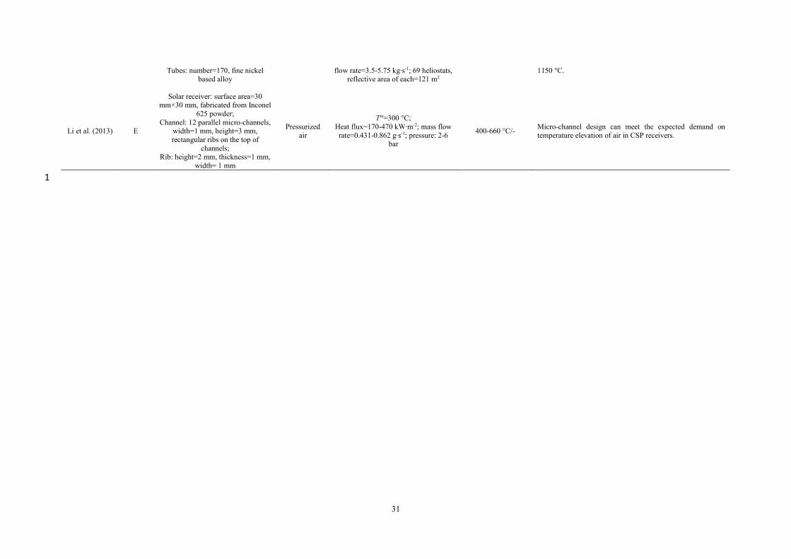
31

Tubes: number=170, fine nickel based alloy

flow rate=3.5-5.75 kg∙s-1; 69 heliostats, reflective area of each=121 m2

1150 °C.

Li et al. (2013) E

Solar receiver: surface area=30 mm×30 mm, fabricated from Inconel

625 powder; Channel: 12 parallel micro-channels,

width=1 mm, height=3 mm, rectangular ribs on the top of

channels; Rib: height=2 mm, thickness=1 mm,

width= 1 mm

Pressurized air

Tin=300 °C; Heat flux=170-470 kW∙m-2; mass flow rate=0.431-0.862 g∙s-1; pressure: 2-6

bar

400-660 °C/- Micro-channel design can meet the expected demand on temperature elevation of air in CSP receivers.

1

32

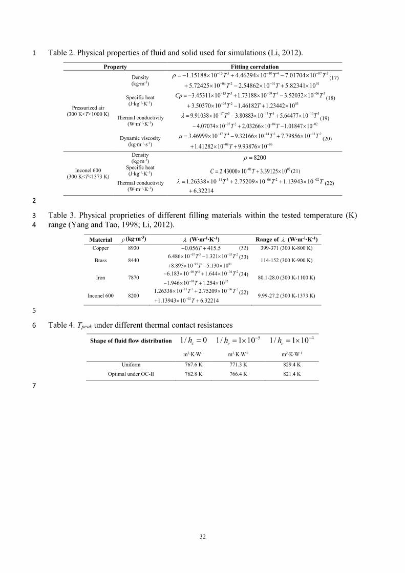
Table 2. Physical properties of fluid and solid used for simulations (Li, 2012). 1

Property Fitting correlation

Pressurized air (300 K<T<1000 K)

Density (kg∙m-3)

13 5 10 4 07 3

04 2 01 01

1.15188 10 4.46294 10 7.01704 105.72425 10 2.54862 10 5.82341 10

T T TT T

ρ − − −

− −

= − × + × − ×

+ × − × + ×(17)

Specific heat (J∙kg-1∙K-1)

13 5 09 4 06 3

03 2 03

3.45311 10 1.73188 10 3.52032 103.50370 10 1.46182 1.23442 10

Cp T T TT T

− − −

−

= − × + × − ×

+ × − + ×(18)

Thermal conductivity (W∙m-1∙K-1)

17 5 13 4 10 3

07 2 04 02

9.91038 10 3.80883 10 5.64477 104.07074 10 2.03266 10 1.01847 10

T T TT T

λ − − −

− − −

= × − × + ×

− × + × − ×(19)

Dynamic viscosity (kg∙m-1∙s-1)

17 4 14 3 11 2

08 06

3.46999 10 9.32166 10 7.79856 101.41282 10 9.93876 10

T T TT

µ − − −

− −

= × − × + ×

+ × + ×(20)

Inconel 600 (300 K<T<1373 K)

Density (kg∙m-3) 8200ρ =

Specific heat (J∙kg-1∙K-1)

01 022.43000 10 3.39125 10C T−= × + × (21)

Thermal conductivity (W∙m-1∙K-1)

11 3 06 2 021.26338 10 2.75209 10 1.13943 106.32214

T T Tλ − − −= × + × + ×+

(22)

2

Table 3. Physical proprieties of different filling materials within the tested temperature (K) 3 range (Yang and Tao, 1998; Li, 2012). 4

Material ρ (kg∙m-3) λ (W∙m-1∙K-1) Range of λ (W∙m-1∙K-1) Copper 8930 0.056 415.5T− + (32) 399-371 (300 K-800 K)

Brass 8440 07 3 03 2

01 01

6.486 10 1.321 108.895 10 5.130 10

T TT

− −

−

× − ×

+ × − ×(33) 114-152 (300 K-900 K)

Iron 7870 08 3 04 2

01 02

6.183 10 1.644 101.946 10 1.254 10

T TT

− −

−

− × + ×

− × + ×(34) 80.1-28.0 (300 K-1100 K)

Inconel 600 8200 11 3 06 2

02

1.26338 10 2.75209 101.13943 10 6.32214

T TT

− −

−

× + ×

+ × +(22) 9.99-27.2 (300 K-1373 K)

5

Table 4. Tpeak under different thermal contact resistances 6

Shape of fluid flow distribution 1/ 0ch = 51/ 1 10ch −= × 41/ 1 10ch −= ×

m2∙K∙W-1 m2∙K∙W-1 m2∙K∙W-1

Uniform 767.6 K 771.3 K 829.4 K

Optimal under OC-II 762.8 K 766.4 K 821.4 K

7