The Bellman equation for minimizing the maximum cost

0362-516.X 89 S3.00+ .oO Z 1989 Pergamon Press plc

THE BELLMAN EQUATION FOR MINIMIZING THE MAXIMUM COST

E. N. BARRON*

Department of Mathematical Sciences, Loyola University of Chicago, Chicago, IL 60626. U.S.A.

and

H. ISHI1-t

Department of Xlathematics, Chuo University, Bunkyo-Ku, Tokyo 112, Japan

(Received 28 July 1988; in revised form 8 August 1988; received for publication 3 October 1988)

Key words and phrases: Essential supremum, minimizing the maximum, Bellman equation, Lp approximations, dynamic programming, optimal stopping.

FORMULATION OF THE BASIC PROBLEM AND INTRODUCTION

WE ARE considering in this paper the following minimax optimal control problem. Given the dynamics on the interval [t, T]

T(t) = x E R”,

(0.1)

(O-2)

the problem is to characterize the value function V”: [0, T] x IR" -+ IR',

where Z[t, T] is the class of measurable functions [: [t, T] + Z C IRe.

This problem arises in at least one important context. Namely, when one is attempting to minimize the maximum deviation from what is desired. In the literature problems in which one has {~h(.s, <(s), c(s)) d.r as cost are typically considered. This represents minimizing cumulative cost. But in many instances this is not good enough. What one actually wants to minimize is the maximum (pointwise) cost. We will study this problem in this paper from the point of view of the value function. The problem of determining a Pontryagin maximum principle to characterize optimal controls when they exist is not considered here.

*Supported in part by grant No. AFOSR-86-0202 from the Air Force Office of Scientific Research. TSupported in part by grant No. AFOSR-85-0315 while visiting the Lefschetz Center for Dynamical Systems, Divi-

sion of Applied Mathematics, Brown University, Providence, Rhode Island.

1067

1068 E. N. BARRON and H. ISHIT

We will prove that V” is the unique, continuous viscosity solution of the quasi variational type inequality

maxlV,“(r,x) + H(t, x, V”(t,x), V, V”(t,x)), y$jh(f,x, .z)/ - V"(r,x)l = 0, (0.3)

if t E (0, T), x E R", with terminal condition V”(T, x) = t$;jh(7; X, z)] on R”, where

and Z(f,X, r) = (z E ZI lMt,x, t)l 5 rJ

Mt, x, r, 9) = min(q *f(f, x, 2); z E Z(t, x, r)1

Notice that we have a lower obstacle given by mi;l/z(f, x, z)l and we also have a constraint

on z through the set Z(t, x, V”). That is, the minimum in the Hamiltonian is calculated over a set which depends on the solution! That is why we (imprecisely) call this a type of quasi variational inequality. The Bellman equation (0.3) explains much of why so little is known regarding minimax problems even though they usually arise more naturally in applications than integral problems. Even calculating the value function numerically in this problem would be a formi- dable task.

If we take the usual definition of the minimum over a set to be + co if the set is empty, we will see in an alternative but equivalent formulation that the function V” also is the viscosity solution of

y-(t,X) + H(f,X, V”(t, x), v,c V”(t,x)) = 0, (0.4)

which still has the constraint on z. The lower obstacle minl/l(t, X, z)l is no longer explicit.

There is no apriori reason to believe that V” is even ck%tuous much less Lipschitz since the controls functions are merely measurable in time. (We will, however, prove that V” is indeed continuous.) Furthermore, whereas the usual cumulative cost problem is almost everywhere differentiable, since it is the integral of an L’ function, the L” norm is not differentiable. Conse- quently, the Crandall and Lions theory of viscosity solutions is required here. Notice also that the Hamiltonian function His not continuous in r (see proposition 2.5 below) so that the extension of viscosity theory to discontinuous Hamiltonians initiated in [5] is needed (see also Barles and Perthame [I]).

In Section 1 we will consider first approximating control problems in which the cost is the Lp

norm of h. The motivation for these approximations is the well known result that the La norm is the limit as p --t co of the Lp norm. In fact, this was our route to discovering the Bellman equation for V”. It is certainly reasonable to guess that the limit function of the Lp approximations is in fact V”. This fact can be proved using the uniqueness of the viscosity solution of (0.3) (or (0.4)), but we provide a direct proof in Section 2. In Section 2 we also prove that V” is a viscosity solution of (0.3) and (0.4).

The approach in Section 1 of using approximating problems is dropped in Section 3 where we take a direct approach. Here we establish a principle of dynamic programming for a slightly more general problem than that considered in previous sections, viz. we do not need to take absolute values of the function h. The dynamic programming principle is established for the essential supremum operator over time. Once the principle of dynamic programming is proved we can show in a more or less standard way that the value function is a viscosity solution of (0.4).

Bellman equation for minimizing the maximum cost 1069

In section 4 we establish first the equivalence of the two formulations of the Bellman equations (0.3) and (0.4). Then we prove that the viscosity solution is unique.

Finally, in Section 5 we consider some further generalizations of our basic problem. In par- ticular, we include payoffs with a running cost as well. We will also see that a simple extension of our basic problem is a generalization of the classical optimal stopping problem. The cost of stopping includes a dependency on the control function. We also put in a remark the corresponding Bellman equation when the controls are restricted to monotone functions. This is a case of the monotone follower problem but with pointwise cost.

Much work remains to be done on this problem. Let us just mention that the convergence of an easily computable sequence to the value function would be the first order of business for applications. The approximations given in Section 1 may not be the best but they are natural. Finding a characterization of optimal controls is an important open problem.

Another open question raised in this paper is the characterization of all operations for which there is a dynamic programming principle.

1. PROBLEMS WITH Lp COST

In this section we consider the following optimal control problem:

subject to

Minimize iP,,,(r) E (3

r Ih(% r(s), &))lP d.s I >

1’p9 Pl 1,

2 = f(r, C(r), C(r)) Ost<rsT,

r(t) = x E rn”,

over the class of controls c E Z[t, T] where

Z[t, T] = (c: [t, T] -+ Z s iRq I[ is Lebesgue measurable)

(1.1)

(1.2)

(1.3)

The set Z is assumed to be compact in Rq. Let BUC([O, T] x R” x Z) be the class of all bounded and uniformly continuous functions

on [0, T] x I?” x Z. We make the following assumption regarding f and h which will hold throughout this paper.

(A) f: [0, T] x IR” x Z + I??” is in BUC([O, T] x IR” x Z) and there is a constant M > 0 such that Ilf(t, x, z) - f(t,y, z)(I I M//X - yII for any x and y E IR”. The function h: [0, T] x I?” x Z -+ R’ is also in BUC([O, T] x I?? x Z).

In this section and in reference to the problem considered in this section we will add the assumption that 0 < inf,,,,,lh(t, x, z>l. In general, our assumptions on f and h are not the weakest possible.

Throughout this paper M will denote a generic constant larger than the bounds on f and h

and the Lipschitz constant for f. We also let ,u, and elf denote moduli of continuity for f and h, respectively. We shall often ignore constants which depend only on the bounds of the functions involved.

Define the value function VP: [0, T] x I?” -+ II?’ by

Vp(t,x) = inf(lP,..(& [ E Z[t, T]).

1070 E. N. BARRON and H. ISHII

The payoff (1.1) is nonstandard in the sense that it is Nevertheless, by transformtion we have the following.

a function of a cumulative cost.

LEMMA 1.1. For each 00 > p L 1, VP E BUC([O, T] x P’) is the unique, continuous viscosity solution of the Bellman

S,( VP) = KP(f, x)

if t E (0, T), x E IF?“,

equation

+ min VxVP(t,x)*f(t,x,z) + -!-(‘~~(~)I)PVY(t,X)j = 0, (1.4) 7.e.z I

VP(T, x) = 0 on IR”. (1.5)

Proof. Define W(t, x) = inf(j:]h(s, c(s), C(s))lP d.s; < E S[t, T]]. Under assumption (A) it is trivial to verify that W is continuous (with modulus depending on p) and bounded. Then, by standard dynamic programming arguments we verify that W is the unique viscosity solution of the problem.

W,(t, x) + mGir$ V, W, x) *At, x, 2) + lh(t, x, z)lpj = 0, t E (0, T), x E W”, (1.6)

with W(T,x) = 0 on iR”. Let K = infr,x,z Ih(t, x, z)lp > 0. Then y(t, x) = K(T - f) satisfies

W,(t, x) + $$l v,W(t, X) *f(t, X, Z) + ]h(t, x, z)lP] = -K + mjnlhlP > 0,

t E (0, T),x E R”, with t&T, x) = 0. By standard comparison theorems we conclude that W > v/ > 0, if t < T.

Let +9(r) = rp on [0, a~) and extend to all of iR’ using the odd extension. If r > 0 p’(r) = prp-’ > 0. Since W > 0 if t < T, we have that W = 9(VP). Therefore, VP > 0 if t <‘T and p 1 1. Using the transformation result in Crandall and Lions [3, corollary I.81 on the equation (1.6), we have that VP is the viscosity solution of

9’( VP) ““;;? x, + t$“z{9’( VP) v, VP@, x) *f(t, x, z) + IhU, x, z)lPI = 0,

t E (0, T), x E R”. Since p’(r) > 0 if r > 0, we conclude that (1.4) must be true. Uniqueness follows by applying the standard comparison result in [3] on the set [0, F] x IR”

with 0 < T < Tand letting i= + T. Notice also that uniqueness is a consequence of the fact that W = 9( VP), W is the unique viscosity solution of (1.6), and 9 is one-one. n

LEMMA 1.2. (i) VP I M(T - t)l’P where A4 = sup,,,,,]h(t, x, z)] < (ii) If p < p’ then VP I Vp’(T - t)@‘-P)‘PP’.

(iii) If 0 I t 5 T and x E IR”, lim VP(t, x) exists. P-m

Proof. (i) Let W(t, x) = M(T - t)“p and put 9 into (1.4) to get

Mj (T _ t)“P-’ [ -1 + m$[ ‘h(t~z”]p]

co.

I 0,

since Ihl s M. Consequently, 9 z VP.


(ii) Let ~(t, X) = VP (T - t)‘P -p)‘pp . Put v/ into the equation for VP to get 2,(w) 5 0 using the fact .2,,( VP’) = 0. We conclude w 1 VP.

(iii) By part (i), 0 I lim sup VP(t, X) 5 M and, if t < T, then we have p--m

lim sup VP(t, x)(T - f)-l’P 5 M.

Further, by part (ii) p-00

VP(t, x)(T - f)+ 5 Vp’(f, x)(T - t)-“P’ if p’ > p.

Therefore, lim VP(t, x)(T - t)-“P exists for t < T, x E R”. Consequently,

lim V”(r, x) = lim ( VP(f, x)(T - f)-“p)(T - f)“P exists V f P-m P-m

Also, since Vp(T, x) = 0 V x E R” and p 2 1, it is clear that lim Vp(T, x) P-m

Define y: [0, T] x R” -+ I?’ by

y(f, X) = lim VP(f, x) = lim Vp(t,x)(T - f)-“p if f < P-m P-m

and y(T,x) = mEi; jh(T,x, 41.

< T.

=o. n

T,

Then, y is at least lower semicontinuous on [0, T) x I?” since it is the supremum of continuous functions:

y(t, x) = sup Vp(f, x)(T - f)-“P. P

Notice that the definition y(T, x) = yJ; jh(T, x, z)l is consistent with the definition of y when

f < T. This follows from the fact that

lim VP(f,x)/(T - f) r-r

I/P = ,‘inri;f [(T - f)-l b[rr Ih(s, r(s), c(s))Ipdrjl/p = E; Ih(TvxAI.

To see that this is true let c(r) E L E Z be fixed and < the associated trajectory on [I, T] starting from x. Then

i:f ((T - f)-’ 1,’ IN& T(s), W)lP d.s 1”’

I [(T- f)-’ j:Ih(s,S(s),i)ipdr]“p

rpu,(T- f) + [(T- f)-l$,‘/h(T,x,z)lpdsj”p.

Since z was arbitrary we have proved that lim_s;p y(t, x) I min Ih(T, x, z)l. For the other side, .TEZ

for any [ E Z[f, T] we have

Im m, CW)l 2 y-j; I4h T(s), z)l

= $j IhlT* r(T)9 z)l + f;$j Ih(s, t(S), Z)l - $; Ih(T, c(T), z)I

L rEi; Ih(T, x, z)l - ,q,(T - s).

Using the arbitrary nature of c we easily conclude.


We easily see that y(t, x) I V”(t, x) if t < T. In fact, for each fixed c E Z[t, T], by Holder’s inequality, for every p 2 1,

(T - f)-“?/h(r, t(r), i(r)&~t,,n 5 Ilh(r, r(r), ~(r))II~tr. rl.

Taking the infimum over < on both sides, we get VP(t, x)(T - t)-l’P I V”(t, x), Vp 2 1. Hence, y(t,x) I V”(f,x), if f < T. However, the reverse inequality is substantially harder to prove because we do not have compactness of the class Z[f, T].

The proof of the assertion y L V” is based on the following lemma.

LEMMA 1.3. Let a > 0 and [ E Z[t, T] and set Q. = (r E [f, T]; Ih(r, r(r), C(r))/ > al where 5 is the trajectory associated to [. Suppose that the (Lebesgue) measure of a,

meas < 6 I T - f, for some 6 > 0. Then there exists a control [E Z[f, T] such that

IN79 f(r), &))I 5 a + P/AM4 for f I r I T,

where <is the trajectory corresponding to [. M is independent of T, f, and 6.

Proof. For simplicity we will take t = 0 in the proof. Then we partition the interval [0, T] as

follows:

0 = f0 < t, < .a. < fk = T, 6 I fj - fj_1 I 26, t/j = 1,2, . . . . k.

Since meas < 6, [fj_l , fj]\C? # @ for j = 1, 2, . . . , k. Let Sj E [tj_1, tj]\a for each j and

define <by

0s) = 6(r) if T E [0, T]\a and fir) = CCsj) ifrE[fj_,,fi]na,j= 1,2 ,..., k.

Then,

]ldGr)/dr - d&r)/drll I M/k(r) - &r)ll + 2Ma(rL OsrsT,

where xa is the characteristic function of a. By Gronwall’s inequality it follows that

II<(r) - f(r)11 5 eMr “e-“1s2A4~a(s) ds I A46, ?

for 7 E [O, T]. 0

Consequently, if r B @_, we have

Ih(7, f(r), fir))/ 5 Ih(7, t(r), c(r))1 + P/,(lk(r) - t(d) 5 0 + &bf’f~)~

and, if T E [fj_, , fj) n Q, then

Ih(r, RT)vfir))I 5 Ih(sj* <(sj), C(sj))I + P/~(IT - SjI + IIt - Ar)ll)

5 0 + P/I(~~ + IIC(sj) - t(r)ll)

I a + &(M6).

We conclude that Ih(r, f(r), c(r))1 5 a + ,~+,(A44 for all 0 5 r 5 T. n

We are now ready to prove the following result.


X) = V”(t, x) if x E I?“, f E [0, T).

Proof. We have already shown that V” 2 y. Now, let t < T and suppose that there is an E > 0 so that y(t, X) I V”(t, x) - 3~.

By definition of y, there is a sequence pj + 00 and ~j E Z[t, T] so that

(1 T Ih(s, t_/(s), Tj(s))IPjds

f >

1 /P,

I V”(r, x) - 2E.

Set GZj = {S E [t, T]; lh(s, <j(S), <Js))[‘J > V”(t, x) - E). Using Chebychev’s inequality we see that

(I ” I~(s, <j(s), cj(s))l’j ds

> I”’ 2 (tIleaS(Qj))“PJ( V”(t, X) - E).

,I

Combining the two inequalities we have that

meaS(Ctj) 5 ( V”(t, x) - 2~

V”(f,x) - & >

pj 3 o asj+ co.

Now we apply lemma 1.3 with 0_ = ~j andj sufficiently large to see that for given 6 > 0 we can find %E Z[r, T] for which

Ih(s, f(r), fial 5 V-0,x) - E + P/m for t I 5 5 T.

But then we have V”(t,x) I V”(t,x) - E + r(lh(B). By choosing p,,(6) < E we have a contradiction. HI

We establish next directly from the definition the continuity of V”. The fact that y(T, x) = V”(T, x) also follows from this proposition.

PROPOSITION 1.5. V” E BUC([O, T] x R”) and V”(T, x) = rj; lh(T, x, z)l.

Proof. Clearly under assumption (A), V” is bounded. We will first establish that V” is continuous in x.

To this end, fix 0 zz t < T and x, ,x2 E I?“. Also fix [ E Z[t, T]. Let T;(e) be the trajectory corresponding to [, with initial position xi, i = 1, 2:

t;(t) = xi e IR”, i = 1,2.

As before, M denotes a generic constant 1 the maximum off and h and 1 the Lipschitz constant off. Then,

so that

max II&(r) - C2(011 5 eMTllxl - x211, ts,+s T

MT, t,(r), C(r)) - h(r, <2(7), 5(Nl 5 ruh(lkl(d - t2(dll) 5 U+Tq - x211),

1074 E. N. BARROX and H. ISHII

for every r E [f, T]. This implies that

I IlMr, t,(s), i(7))llLmf,. rl - llN7y G(7), i(7))llr-tr.nI 5 kAe‘Wl - sy~ll).

We conclude that for 0 5 t 5 T and x, ,x2 E IF?“,

I V”(t, x,) - V”(t, x,)1 5 iUh(eh’rll_V, - x,11).

Thus V” is continuous in .Y.

(1.7)

To establish that V” is continuous in t, fix x E R” and < E Z[O, T]. Also, fix 0 I t, < f, 5 T. Let Ti be the solution of

2 = f(s, ri(r)3 C(Ir)) OIti<sIT,

&(f;) = x e rn”, i = 1, 2.

Then, by standard results in ODES we have II<, - XII 5 M(tz - f,), where we are assuming

that Ilf(t, x, z)ll I M. It follows that for every r E [f2, T] we have

ll5,(7) - L(7)ll 5 e “f’ll<,(tz) - xll I M(t, - t,)e”Y

Consequently, we have for h that

147, t,(7), C(7)) - h(7, b(7), i(7))l 5 &@fehfr4

for 7 E [tz, T], with 6 =I f2 - t, . But then

k(r, C,(7), i(7)&-[,,, rl 2 llh(7, T,(7), I(7)lh2, iy

1 b(7, &(7), ~(~))llLB~,Z, rl - dMeMT4, and

llh(r, t,(7), C(7))// L-[rz, rl 5 1147, b(7), C(7))llLlLf2, n + hOfebfT@.

Next, let 1;1 be the trajectory on [tz, T] given by

$ = f(7, v(7), c-(7 - 6)) Ost,<TsT,

q(tJ = x E I??“.

(1.8)

(1.9)

Then, for every 7 E [fz , T],

II d5;(7 - 6) dr

- 37) I/

5 llf(7 - 6, <,(7 - a), c(7 - 6)) - f(7, V(7), i(7 - @)ll

5 MllT1(7 - 6) - Il(7)ll + P@).

Using Gronwall’s inequality we get that

Ikl(7 - 4 - a(7)ll 5 eMTIIIT,(t,) - XII + ~f@)l, t, I 7 5 T.

Hence,

147 - 6, <t(r - a), c(r - 4) - 47, q(r), ((7 - 4)l 5 deMT(Md + ~~(6)) + a),


for every r E [tz. T]. Using this, we get

llMr* r,(r), Gr))II L”[r,, T-61 5 IlMr, q(r), a7 - m11,=q,,, 7J

+ ph(eMF(Ma + p,(d)) + 4.

Putting the pieces together, (1.8) gives us that

V”(t,, X) 1 Vm(fZ, x) - flh(MehfF6).

Then (1.9) and (1.10) yield

(1.10)

V”(t, x) 5 V”(t2, x) -t pc,(e MF(MG + p,(d)) + 6), T-k t,

if tz 5 - 2 .

Note that this implies that [t, , T - 61 U [tz, T] = [t,, T]. We conclude that

I v”(f,, 4 - ~“(4, -4 5 i.4deMFW~ + i+,(4) + 4.

This proves that V” is continuous on [0, T] x R”. In view of (1.7) we have left to show that

lim V”(t, x) = $; Ih(T, x, z)l. (1.11) 1-F

To see that (1.11) is true given any z E Z for c E Z[t, T] with ((7) = z and corresponding trajectory < we have

I’“(t, x) 5 Iy;.F IMr, t(r), c(r))1 5 p,,(M(T - t)) + Ih(T, x, 41.

We conclude that lim_s;p V”(t, x) 5 mEi; Ih(T, x, z)l.

For the reverse inequality we have that for every r; E Z[t, T]

IIN T(7), R7NII ~-[r, rl 2 lW-, K? W))t

1 min Ih(T, x, ~$1 - ,uh(M(T - I)). zsz

Consequently, lim inf V”(t, x) r $2 Ih(T, x, z)l. This completes the proof. H I-F

We see that y = V” on [0, T] x IR”. From the fact that y = V” we also have y E BUC([O, T] x I?‘). This fact can also be proved directly from the definition of y.

2. THE BELLMAN EQUATION FOR V”

In this section we will derive the Bellman equation for V” by using the fact that V” is approx- imated by VP. It is important to notice that the theory of viscosity solutions to first order problems is critical here since we do not know that y, V”, or VP are at all differentiable at any point.

The motivation for the derivation of the Bellman equation for V” is the following proposition which is a statement of a penalty method in mathematical programming.


PROPOSITION 2.1. Let (Y, ,8 be continuous on 2, where Z E I? is compact, and let ,U and v E (0, m). Then with Z(r) I (z E Z: I/I(t)/ % r)

where the min on the right is taken as + 00 if Z(v) = 0.

Proof. If v < mei”, @(z)I then Z(v) = 0 and the proposition obviously holds in this case.

Thus we assume that v L r$t //3(z)/. Then Z(v) is closed and hence compact in Z.

In Z(v), IP(z v 5 1 and I/&z)//v > 1 if z E z\Z(v). We have

Now, let .zp E Z satisfy

(2.1)

(2.2)

Let i E Z be a limit point of (z,). Indeed, we may assume without loss of generality that z, --) 2 as p -+ co. We claim that Z E Z(v). To see this, suppose that 2 $ Z(v). Then, for large p, z,, $ Z(v) since Z(v) is closed. So @(zJ~/v > 8 for large p for some B > 1. But then

& ) + .! IB(zJ pp 4 + w P

[ 1 asp + m.

P v Since Z(v) # 0, there is at least one z. E Z(v). For this z.

a(q)) + i IPko)l pp -+ cY(zo) [ 1

asp -+ 00. P v

(2.3)

(2.4)

However, (2.3) and (2.4) taken together contradict (2.2), the minimizing property of (zJ. Con- sequently, i E Z(v).

We next claim that 2 is a minimizing point for Q: CY(.?) = z~Epj a(z). Again, suppose not.

Then, there exists z’ E Z(v) so that

cu(n > cu(z’) = zyin”, a(z).

We have that


But this last inequality again contradicts the minimizing property of 1~~1 in (2.2). Thus, our claim is proved.

Next, using (2.1) we have

But, since IP(z,)l/v 2 0,

By previous arguments,

lim sup f_~(zJ = a(.?). P-m

Combining this with (2.5) completes the proof. n

Motivated by proposition 2.1 we have the following.

PROPOSITION 2.2. V” is a viscosity solution of the equation

Km@, x) + H(t,x, V”(f, x), v, V”(t, x)) = 0,

if t E (0, T), x E R”, with

V”(T, x) = mj; Ih(T, x, z)l on R”

where

and

Z(f, x, r) = lz E Z I Ih(t, x, z)l 5 4

(2.5)

(2.6)

(2.7)

H(t, x, r, q) = minlq -f(t, x, 2); .z E Z(f, x, r)l. (2.8)

We will refer to H as the Hamiltonian of the problem. Before we prove the proposition we must define what we mean by viscosity solution when the Hamiltonian is discontinuous and consider several properties of H.

We will denote by Bs(f, x) the ball of radius 6 > 0 centered at (f,x). Now we begin by establishing some properties of Z(f, x, r).

LEMMA 2.3. If r 4 r’, then Z(f, x, r) c Z(f, x, r’). (ii) If r < r’, x E II?” and 0 5 f c T, there exists 6 = 6(r, r’) > 0 such that

Z(s, _v, r) C Z(t, x, r’) for every (s, y) E BB(f, x).

Proof. (i) is obvious. To prove (ii) fix 6 > 0 so that p,,(B) 5 r’ - r. Let (s, _v) E B,(t, x) and z E Z(S, Y, 4. Then h(f, x, z) 5 h(.s, y, z) + &(B) I r + r’ - r = r' . That is, z E Z(t, x, r’). W

The next lemma follows immediately from lemma 2.3.


LEMMA 2.4. (i) If r I r’, then H(t, X, T, 4) L H(t, X, r’, q). (ii) If r < r’, x E R” and 0 5 t I T, there exists a 6 = 6(r, r’) > 0 such that

MS, Y, rr 4) 2 Mt. x> r’r 4) for any (s, y) E &(f, x).

Since it is not clear that H is continuous we will need the upper and lower semicontinuous envelopes of H. They are defined, respectively, by the following functions:

H*(t, X, rr q) = lim_sup lH(s,_v, P, m): Is - tl + Ilx - yll + Ir - PI + 114 - mll 5 4,

and

H,(t,x, r, q) = lim_$f (H(s,y,p, m): Is - fl + [Ix - y/ + Ir - pi + 114 - ml/ I ~1.

PROPOSTION 2.5. We have

and H*(t, x, r, q) = H(t, x, r - 0, q),

H&,X, r, 4) = H(t,x, r + 0, 4).

Proof. We will only prove the second assertion since the first assertion is entirely similar. To this end, fix (t, x, r, q) E [0, T] x R” x [0, 00) x R” and fix E > 0. By lemma 2.4, we can find 6 > 0 such that

H(s, Y, P, 4) 2 H(f, X, P + ~12, q)

2 H(f, x, r + E, q) for any (s, Y) E &(f, x) and p 5 r + e/2.

Consequently, H(.s, y, p, m) 2 H(f, x, r + E, q) - ME for (s, y) E B,(f, x), p I r + ~12 and m E B,(q). So, H,(f, x, r, q) 2 H(t, x, r + E, q) - ME. Since E was arbitrary, we have H,(f, x, r, q) L H(f, x, r + 0, q). However, directly from the definition of H, we have that H,(f, x, r, q) 5 H(f, x, r + 0, q). This completes the proof. n

We now state precisely the requirements for a viscosity solution. We will use the extended viscosity theory in lshii [5] in view of the fact that His not continuous in r.

Definition. Let G be a function on (0, T) x I?” x R’ x I?“, possibly taking the values + ~0 or - m. A continuous function u on (0, T) x IR” is a viscosity solution of

u,(f, x) + G(f, x, u(f, x), V,Mf, x)1 = 0, if:

(i) for any 9 E C’((0, T) x IF?“) so that u - cp has a minimum at (s, y) E (0, T) x I?” we have

MS, Y) + G&s, Y, ~6, Y), V,V(S, Y)) 5 0,

(That is, u is a viscosity supersolution); (ii) for any QY E C’((0, T) x I?“) so that u - cp has a maximum at (s,y) E (0, T) x R” we

have

MS, Y) + G*(s, Y, ~6, Y), Y&s, Y)) 1 0,

(that is, u is a viscosity subsolution).


This definition may be extended to include (possibly) discontinuous viscosity solutions by taking the lower semicontinuous envelope u,(t, x) = lim inf u(s, y) (respectively, upper semi-

S-rl.Y-rX continuous envelope u*(t, x) E lim sup u(s, y)) of the locally bounded function u in the defini-

s-r.y-X tion of viscosity supersolution (respectively, subsolution). In our case we have already proved that V” is continuous so that this is not required here.

We may assume in the definition that the minimum or maximum is strict. Further, by considering +(t, x) = cp(t, x) - (u(s, y) - rp(s,y)), we may always assume that the minimum or maximum is zero. Finally, if one is considering the initial value problem rather than the terminal value problem then the inequalities in the definition should be reversed.

We are now prepared to present the following.

Proof of proposition 2.2. Since we know that VP * V” uniformly on compact subsets of (0, T) x ll?” the proof of this proposition follows from a stability result for discontinuous Hamiltonians in Ishii [5, pp. 52-531. A result of Barles and Perthame [I, theorem A.21 allows one to dispense with the requirement of uniform convergence. We need to verify that for 4 = (41, Qz) E R”“, (t, x, r) E (0, T) x I?” x (0, co), we have

= 41 + H*(t,x,r,q,) = QI + mt,x,r + O,q,) (2.9)

and

= 41 + H*(t, x, r, 92) = Ql + w, x, r - 0.42). (2.10)

To prove (2.9), we first note that if Z(t, x, r + 0) = 0 then (2.9) will obviously hold. So assume that Z(t, x, r + 0) f 0. Since

; (h(J;Al)pp ~ o

(we may assume p 2 0), we have

m, -f&y, Z) + p 1 (h;. z”>“l

COnWUently, the lim inf in (2.9) is always bounded below. We have

= 41 +

+

min ZEZ I 42 *f(t, xv z) + (m, - 42) ~.fu,X,Z) + (f(s,y,z) - f(t,x,z)) * m,

l ‘h(t,xs z)’ + ('W,Y, z)’ - ‘W, x, z)‘) 5 r + (P - d

(2.11)


From the preceding equality it is easy to verify using proposition 2.1 and the continuity off, h and the min operator that (2.9) must be true.

The proof that (2.10) holds is similar and is omitted. Once (2.9) and (2.10) are established we use the fact that V”(f, X) = lim VP(t, x) and the

P-m fact that VP is the viscosity solution of (1.4). The Hamiltonian in (1.4) has H* (resp. H*) as the upper (resp. lower) semicontinuous envelope as p + co. We may then apply the results of lshii [5, pp. 52-531 to conclude the proof. n

We also have the following proposition.

PROPOSITION 2.6. V" is a viscosity solution of the equation (obstacle problem).

max] K”(t, x) + H(t, x, V”(t, x), V, I/“@, x)), m$r Ih(t, x, z)l - V”(t, x) 1

if t E (0, T),x E I?“, with V”(T,x) = r$; Ih(T,x, z)j on R”.

= 0, (2.12)

The proof of this proposition is similar to that of prop 2.2 but we will give the details of a direct proof for completeness. The definition of viscosity solution here is an obvious extension of that given earlier. Also, refer to proposition 4.1 to see that the two formulations (2.12) and (2.6) are in fact equivalent.

Proof. Let (p E C’((0, T) x IR”) be so that V” - u, has a (strict) local minimum at the point (s,y) E (0, 7’) x Pi?“. Without loss of generality we may assume that the minimum is 0 so that cp(s,y) = V”(s, y) > 0. Then, for large p, since VP -+ V” uniformly on compact subsets of (0, T) x IR”, there exists a point (f,, , xJ E (0, T) x I?” satisfying VP - rp has a minimum at UP, -Q,), v($, , xP) > 0, and VP9 q,) -+ (s, y) asp --+ 00. Since VP is the viscosity supersolution of (1.4), we have

~,U,, xp) + min ZCZ

V,vUp, xp) -f(t,, xp, 2) + j ’ (‘“;~;~;,‘)p~(~p,xp)j I 0. (2.13)

Since

we have

rp,(~p,Xp) + $$ t VA@,, xp) -_f(f,, xp’al

So, there exists a constant K > 0 such that


Since p L 1, this gives us that

Letting p --* 00

Z(h Y, rp(s, Y)) f We have from

min ZEZ

1 P (

min,.zIh(~p,~p,z)I ’ = K d&9 xp) > qE-gxp)

we conclude that cp(s, Y) 2 min Ih(s, Y, z)j. This also implies that ZEZ

0. the continuity of h, rp, and Dv that if E > 0, then

for large p. From (2.13) and the preceding inequality it is easy to verify using proposition 2.1 that by letting p + 00

rp,(h Y) + mid VA@, Y) *.f(s, Y, z); z E Z(s, Y, cp(s, Y) + 2~11 5 8, v & > 0.

Consequently,

e&Y) + min ( V,&,Y) -f&y, z>; z E Z(S,Y, ds, y) + 011 5 0.

We conclude using proposition 2.5 that V” is a viscosity supersolution of (2.12). Let (Q E C’((0, T) x IR”) be so that V” - (D has a (strict) local maximum at the point (s,y).

As before, we may assume that the maximum is 0 so that &s, y) = V”(s, y) > 0. For large p, there exists a point (tP, xJ satisfying: VP - (p has a maximum at (fP, x,), ~(t,, xJ > 0, and

($,x,) -+ 6,~) asp -+ 00. Since VP is the viscosity solution of (1.4), we have

cp&,x,) + min ZeZ

V,(~(~,,X,)~~(~~,X~,Z) + p ’ ~“~~;+$)“e$, , xP)] L 0. (2.14)

Suppose that &s,y) > $; Ih(s, y, z)l since if &,y) = t$ Ih(s, y, z)l there is nothing to

prove. Then, for each p sufficiently large, we also have &t,, xp) 1 $; Ih(tp, xp, z)l so that

both Z(s, Y, V(s, y)) and, for large p, Z(t,, xP, Vm(fP, x,,)) are nonempty. By continuity, we have from (2.14) that if 0 c E < &r,y), then

c4hY) + $; t

1 PGY, dl + E V,ulhy) -f(s,y, z) + p ( dS,Y) - E > 1 pv(s y) + E 1 o

’ , for large p. Using proposition 2.1, by letting p --t CO we conclude as above that

V,(&Y) + M&Y, &,Y) - 0, V,V(.%Y)) 1 0. (2.15)

Consequently, V” is also a viscosity subsolution of (2.12). This completes the proof. n

3. THE PRINCIPLE OF DYNAMIC PROGRAMMING

in this section we will show that a dynamic programming principle holds for our minimax problem. This will provide a more direct way of approaching general minimax problems of the type considered in this paper.


We will generalize our original problem slightly by considering the value function V: [O, 7-l x IF?” -+ I?’ defined by

with the same dynamics as before

2 = f(7, r(7), ((7)) OstsT, (3.2)

r(t) =x E IR”. (3.3)

We have dropped the absolute values from h. Define more generally the set

Z(t, x, r) = (z E Z; h(t, x, z) 5 r),

and define the Hamiltonian function H: [0, T] x I?” x IR’ x IR” + IR’ by

H(t, x, r, 9) = minlf(t, x, 2) - q; z E Z(t, x, f)) (= + 03 if Z(t, x, f) = 0).

Then the lemmas 2.3, 2.4 and proposition 2.5 still apply to the set Z and the function H. We now have the following.

PROPOSITION 3.1. (i) V E BUC([O, T] x IF?“). (ii) Let 0 5 t < s 5 T, and x E R”. Then

V(t, x) = ~ .in& 5l maxless.sup h(r, T(7), c(7)), W, (WI. tliTaS

(3.4)

Remark. Part (ii) of the proposition is the Principle of Dynamic Programming.

Proof. Part (i) is proved as in proposition 1.6. As for part (ii) let [ E Z[t, T]. Define [, E Z[t, s] and Cz E Z[.s, T] as the restriction of [ to the interval [t, s] and [s, T], respectively. Let < be the solution of (3.2)-(3.3) for the control [. Then,

= max(ess.sup h(7, l(r), c,(r)), “,“sf;g h(7, r(7), L(7))l ,STiS

1 maxkss.sup h(7, r(7), cd7)), VA W)l r5,SZ.v

L I hi Il max(ess.sup h(7, r(7), C(7)), W, W)L fZS,bS

Consequently,

V(I, x) B I i$ s1 maxfess.sup h(7, T(7), c(r)), W, W)I. E * f577sS


For the reverse inequality, suppose we are given controls c, E Z[t, s] and (I E Z[s, T]. Define the control [ E Z[t, T] by

C(r) = Cl(r) iftlT<S and C(r) = (z(r) ifs5 r~ T.

Let < denote the trajectory on [t, T] corresponding to the control C;, Then,

maxless.sup h(r, C(r), C,(r)), ess.sup h(r, r(r), Mr))] ,575s SSTST

= ess.sup h(r, r(r), C(r)) 2 V(t, x)

fS7ST

So, since this is true for any cz,

maxless.sup h(r, C(r), C,(r)), I+. T(s))1 2 W, x). lz%TzzS

Taking the inf over Z[t, s] we finally get

inf maxless.sup h(r, c(r), C,(r)), I+, T(s))] L V(t, x). n I E m. 4 ,dTSS

It is normally the case that once a dynamic programming principle has been established one can use this principle to prove that the value function is a viscosity solution of a Bellman equation. This has been carried out for standard control problems and differential games in Lions [6], Barron et al. [2], Evans and Souganidis [4], et al. We will next provide a proof of this fact for our problem using this method.

THEOREM 3.2. The value function is a viscosity solution of the Bellman equation

with v, + H(t,x, v, V,V) = 0 in (0, T) x I?” (3.5)

V(T, x) = r;n,‘q h(T, x, z) ifxE IR”. (3.6)

Proof. Let 9 E C'((0, T) x II?") and (s, Y) E (0, T) x IR” a point at which V - cp has a (strict) local maximum (of 0). Let us suppose that

(Dr + MS, Y, rp(s, Y) - 0, V,(P) < 0 at (s, Y). (3.7)

We will derive a contradiction. If (3.7) holds, then there is a 6 > 0 for which

$5 + Ns, Y, (PCs, Y) - 46, V,co) < - 46 at (s,Y).

There is z E Z(.s, y, cp(s, y) - 46) such that co&, Y) + f(s, y, z) - V,cp(s, y) c - 36. By definition of Z(s, y, cp(s, y) - 46) we also have h(s, y, z) I &s, y) - 46. Using continuity and replacing 6 by a smaller 6 if necessary, we may assume that

p,(t, x) + f@, x, z) * v,coct, x) 5 - 26 and W, x9 z) 5 &Y) - 36 (3.8)

for any (t, x) E Bb(.s, y). Define the control [ E Z[s, T] by C(r) = z and let r be the trajectory associated with [ starting from y at time s, i.e. r(s) = y.


Choose 0 E (s, T) so that (7, c(r)) E B&Q, y) for all s I 7 I CT. From the first part of (3.8) we have

9,(7, ((7)) + f(7, T(7), i(r)) * V,cp(r, ((7)) 5 - 23 v 7 E (s, a).

Integrate this last inequality from s to o to get 0 2 9(a, r(o)) - 9(s,y) + 26(a - s). From the second part of (3.8) we also have h(7, r(r), I;(r)) I c&y) - 26, for every r E (s, a). Using the facts V 5 9 and V(.s,y) = 9(s,y), we get

V(o, ((a)) 5 9(a, ((0)) 5 96,Y) - 240 - 4 < W,Yh and

ess.sup Mr, <(r), C(7)) 5 cp(s, Y) - 26 < W, Y). tsT*o

Taken together we have a contradiction of the principle of dynamic programming in proposition 3.l(ii). Consequently we must have

9, + H(s, YT 96,Y) - 0, V,9) 2 0 at thy),

so that Vis a viscosity subsolution of (3.5). Now we let 9 E C’((0, r) x IF?‘) and (s, y) E (0, T) x R” a point at which V - 9 has a (strict)

local minimum (of 0). Let us suppose that

9I + H(s, Y, 96,Y) + 0, V,9) > 0 at @,Y). (3.9)

We will again derive a contradiction. There is a 6 > 0 for which

9As, Y> + f&Y, 9hY) + 36, V,9) 2 36 at (s, Y).

By lemma 2.4(ii) we may assume that

9,,(r, x) + H(f, x, 96, Y) + 26, v,9(t, x)) 2 26 for any (7,x) E B&(s,y). (3.10)

Let [ E Z[s, T] be arbitrary and let < be the trajectory on [s, T] starting from y at times, i.e. r(s) = y, corresponding to the control [. Choose cr E (s, 7) so that (7, c(r)) E B,(s, y) for s I 7 I Q. We have two cases to consider:

or

ess.sup h(7, r(7), i(7)) > 96, y) + 6 = I+, Y) + 6, SS;r50

(3.11)

ess.sup h(r, r(r), c(r)) 5 9(.s,y) + 6 = V(s,y) + 6. SST50

(3.12)

In case (3.12) holds by (3.10) and continuity we have

9,(7, T(7)) + f(7, r(7), C(7)) * V,9(7, T(7)) 2 6 for a.e. 7 e (s, 0). (3.13)

Notice that Z(7, r(r), 9(s, y) + 6) # (2J if (3.12) is true. Therefore, integrating (3.13) we obtain (a - s)6 5 9(a, <(a)) - 9(s, Y), so that

WY) < US,Y) + (0 - M 5 va, r(N). (3.14)

If (3.11) is true then, of course, esssup h(r, r(r), c(r)) - 6 > V(.s,y). Then (3.11) and (3.14) SST50

together yield

V(s,y) 5 max(V(a, <(a)), ess.sup h(7, T(r), c(r))] - 6min(o - s, 1). SSfd,J

Bellman equation for minimizing the maximum cost IO85

Notice that 0 can be chosen independent of [. Thus, by using the fact that c was arbitrary we take the inf of both sides and derive a contradiction to the principle of dynamic programming. We conclude that V is a viscosity supersolution of (3.5) as well. II

Remark. Using the dynamic programming principle it is also possible to prove directly that V is the viscosity solution of

max{ vl(t, x) + H(t, x, V(t, x), V, V(t, x)), $; h(t, x, z) - v(t, x)) = 0.

That these two formulation are equivalent will be proved in the next section.

4. UNIQUENESS OF THE VISCOSITY SOLUTION

In this section we will establish that there is exactly one viscosity solution of the Bellman equations considered in this paper. We begin by establishing the equivalence of two formulations of the Bellman equation.

PROPOSITION 4.1. The function u E BUC([O, T] x iR”) is a viscosity solution of

U,(f,X) + H(t, x, u(t, x), V,u(t,x)) = 0.

if and only if u is a viscosity solution of

maxb#, x) + Mt, x, u(t, x), V,u(t, x)), t$rj h(t, x, 2) - u(t, x)1 = 0,

if t E [0, T), x E IR”.

(4.1)

(4.2)

The advantage of introducing (4.2) is to make explicit the appearance of the lower obstacle min h(t, x, z). The formulation (4.2) is especially useful in the case when h is independent of z ZEZ (see the remark following the proof).

Proof. Let u be a viscosity solution of (4.1). Suppose that min(u - cp) = u(s, y) - &, y) = 0 with a, E C’. Then

GG%Y) + M&Y, P$%Y) + 0, VA.% Y)) 5 0.

It follows that Z&y, u(s,y)) # @ so that min h(s,y, z) - u&y) I 0. We conclude that ZEZ

and hence u is a viscosity supersolution of (4.2). The fact that u is a viscosity subsolution of (4.2) is trivial. Now let u be a viscosity solution of (4.2). The fact that u is then a viscosity supersolution of

(4.1) is immediate so we have only to show that u is a viscosity subsolution of (4.2). To see this, suppose p E C’ with u - p attaining a local max (= 0) at the Ijoint (s, y) E (0, T) x IR”. Since u is a viscosity subsolution of (4.1) we have that

maxM.5 u) + H(s, Y, ~6, Y) - 0, V,cp(s, Y)), psi; h(s, Y, z) - ~6, u)l 1 0. (4.3)


If p,(s,Y) + H(s, Y, cp(s, Y) - 0, V,q?(s,Y)) c 0 then we must have that there is some 6 > 0 so that p&y) + H(s,y, (D(s, y) - 6, V,cp(s,y)) I -6. Consequently, there is z E Z(s,y, &,y) - 6) so that h(s, y, z) 5 &,y) - 6. On the other hand, (4.3) tells us that we must have min h(s, y, z) - c$s, y) 2 0. This is a contradiction. We conclude that

ZGZ

MS, Y) + m, YI $a* Y) - 0, V,&, Y)) 2 0

and so u is a viscosity subsolution of (4.2). n

As a result of this proposition we need only establish uniqueness for one of the formulations. We will do this in the next theorem.

Remark. When the function h = h(r, x) is independent of z we have an optimal control problem with optimal stopping and with continuous control. The Bellman equation is the variational inequality

max] K(t, x) + min V, v(t, x) *f(t, x, z), h(t, x) - u(t, x)) = 0. ZCZ

This is a standard problem with continuous obstacle h.

THEOREM 4.2. There is at most one viscosity solution u E BUC([O, T] x iR”) of (4.1) satisfying u(T, x) = min h(T, x, z), x E I?“.

ZCZ

Proof. Suppose that u and v in BUC([O, T] x P’) are both viscosity solutions of (4.1) and both satisfying the terminal condition. Let R > 0 and g, E C’(?‘) satisfy Ordg,(r)/drs l,g,(r)=OforrrR,and limg,(r)= +co.Fixp>Oandset

r-m

v’(l,x) = v(t,x) + /3gR(1X]) + M/?(7-- f) + $.

Then F L v and J is a viscosity supersolution of the equation

P F, + H(t,X, J, v,c) + - = 0.

t2

We will indicate how this is checked formally. We have

J, + H(?, x, 0, v, c) = v, - Mp - t2 Q+H dg, X t,x,v, v,v+p--

dr 1x1

+ H ‘h X t,x, v, V,v + p------ dr 1x1

I v, - IV@ - $ + H(t,x, v, V,v) + M@

P = --* t2

Now, put w(l, x, y) = u(t, x) - J(t,y). Then, since u is a viscosity subsolution and P is a viscosity supersolution we see (e.g. [S]) that w satisfies in the viscosity sense (i.e. w is a viscosity

Bellman equation for minimizing the maximum cost

subsolution)

1087

P w, + H*(t, x, w + v’(t, y), v, w) - H*([, y, - w + u(t, x), - vy w) - - e 0.

t2

Let E > 0, and consider the function defined by

qt, x, Y) = W(f, x,y) - ; IIX - YI12 = fdt, 4 - F(l, Y) - & IIX - YI12.

The function 0 attains a maximum at some point (< R, p) E [0, T) x IF?’ x IR”. We have that

& lb - PII + 0 as e 10,

and u(t; X) - J(t; 9) + max(u - VT as E 10.

Now, suppose that max(u - G) > 0. Then T > ?> 0 and, as a consequence of the definition of viscosity subsolution, using the test function 112~ /Ix - yl12 we have

H* (

t;n, w(t;x,~) + J(i;+ -J) > (

-H, <j,-w(r;a,p)+~(r;+-J) >

-+O.

(4.4)

We may assume that w(C X, p) > 0 so that w(< X, p) + v(< p) = u<< .F) > C(< p) = w(C X, p) - u(< x). Now, choose r, and r2 E IF?’ so that u(E X) > r, > r, > P(< p). We may assume that rl - r, 2 CY > 0 for some constant (Y by choosing E > 0 sufficiently small. Then

H* (

t;x, u&x), i(x - J) > (

= H t;x, u(t; x) - 0, ; (X - y) > (

5 H t; X, r,, L (Jc - &

J) >

and

H, (

t;~,C(r,~+y) > (

= H t;~,J(t;y) + O,+) ) (

2 H <JJ,,~ ‘(x - J) >

.

Next, using lemma 2.4(ii) we may choose 6 > 0 so that H(< y, r2, q) L H(< X, r, , q) for every y E B,(I) and q E /R”. We may assume that I/X - p[I I 6. Therefore, combining these remarks with (4.4) we obtain

P < H fi- r;_v,r,, $-y, =0,

obviously a contradiction. We conclude that it must be true that max(u - G) I 0. Thus, since p was arbitrary, u I v. By an entirely similar argument we get v I U. This completes the proof. H

Remark 1. Possibly the easiest way of proving that the Lp approximations converge to V”, that is, that y(t,x) E V”(t,x), is by using the uniqueness theorem. In other words, prove directly that y and V” both are viscosity solutions of the Bellman equation and then apply theorem 4.2.


2. Theorem 4.2 also shows that

qt, x) = inf ess.sup H(s, T(T), C(T)) = inf SUP h(T, t(T), c(T)). TEZII.lJ rsrs7 c~Z[r,TjrarsT

This true because both sides of the equality are viscosity solutions.

5. GENERALIZATIONS TO PAYOFFS WITH RUNNING COST

In this section we will state without proofs some generalizations of our previous problem. We begin with the inclusion of a running cost.

Consider the following optimal control problem

7 Minimize ess.sup g(s, r(s), c(s)) d.s + h(r, r(r), c(r))

IITST f > 3 (5.1)

subject to

((1) =x E IR”, (5.3)

over the class of controls c E Z[t, T]. This problem generalizes those of previous sections in that we are including the running cost g E BUC([O, T] x R” x Z).

The value function for this problem is given by

V(l, x) = inf ess.sup (S T

&'(S, r(s), c(s)) d-v + h(Tt r(T), c(T)) > .

fEzt1,r-l rs,raT f

THEOREM 5.1. (i) V E BUC([O, T] x IR”);

(ii) V satisfies the dynamic programming principle: for any 0 < E < T - t,

T

V(1, x) = r E Z[f, Ice]

g(% c(s), c(s)) d.s + h(r, c(r), c(r)) , I

(iii) V is the unique viscosity solution of

with v + H(1, x, v, v, V) = 0 in (0, T) x R”

V(T, x) = min h(T, x, z) ifxE R”, ZGZ

where H(t, x, r, q) = minlq +f(t, x, z) + g(t, x, z); z E Z(t, x, r)) and = + m if Z(t, x, r) = 0.

The proof of Theorem 5.1 is given anaolgously to previous sections and is omitted.


Finally, as a direct generalization of the standard deterministic optimal stopping problem (for example, see Barles and Perthame [l], or Lions [6] consider the value function

17 V(f,X) = inf ess.inf

(1 g(s, r(s), C(s)) d.s + h(r, r(r)* C(r))

rEZ[f.7j raTaT I > .

The cost of stopping at time T involves the control function i and is, in general discontinuous. Barles and Perthame [l] consider optimal stopping problems with discontinuous cost and show that the value function is not necessarily continuous. But, in our case V is shown to be continuous as in Section 2. For this problem we have the following.

THEOREM 5.2. (i) V E BUC([O, T] x R”); (ii) V satisfies the dynamic programming principle: for any 0 < E < T - t,

i (i ,

V(f,X) = inf min ess.inf g(s, T(s), T(s)) d.s + h(r, C(r)* I;(r)) 9 f E Z[f, r+&J ISTi*+E I >

(iii) V is the unique viscosity solution of

F + H(t,x, V, v,v) = 0 in (0, T) x IF!’ with

UT, xl = ~j; h(T, x, z) if x E IR”,

where H(t, x, r, q) = minlq .f(t, x, z) + g(f,x, z); z E Z fl (h(r, x, z) L r] and H = + CO if z n (h(t, x, z) L r) = 0.

Remark. It was pointed out to us by W. H. Fleming that the last problem is qualitatively easier than the preceding problems in that we are using the inf operator on both T and c.

Remark. In the case of a stochastic minimax problem we have

where dr(r) = f(r, c(r), C(T)) dr + ~(7, <(T)) dw(r), if t < T 5 T, r(f) = x, w(e) is standard Brownian motion and 0 is a stopping time with values in [f, T]. Then using an extension of the current theory of viscosity solutions to second order PDE, we would obtain the Bellman equation

max( V,(f, x) + +mTDz v + min 2 E w.x. VU.X))

f(f, x, z) * v, Vf, x), $; h(f, x, 2) - V(f, x)) = 0,

(or equivalently, V, + *acrTpV -t H(f,x, V, V, V) = 0) if f E [0, T],x E IR”, with V(T,x) = min h(T, x, z) on IR”. Of course one could also consider r = r(f, x, z). Zt-Z


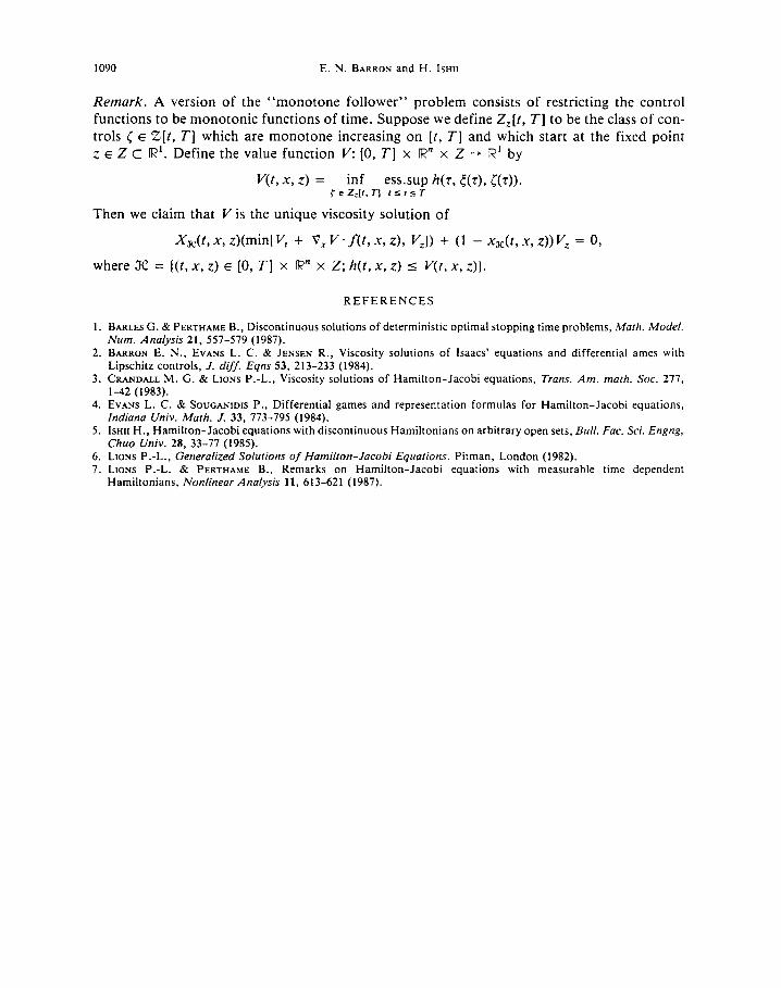
Remark. A version of the “monotone follower” problem consists of restricting the control functions to be monotonic functions of time. Suppose we define Zz[f, T] to be the class of controls L: E Z[t, T] which are monotone increasing on [t, T] and which start at the fixed point z E Z C R’. Define the value function V: [0, T] x IR” x Z -+ IR’ by

V(f, x, z) = inf ess.sup h(r, T(r), c(r)). rEZ;[I,7l ts;ts;r

Then we claim that V is the unique viscosity solution of

X&t, x, z)(min] K + V, v+f(t, x, z), v,l) + (1 - x&t, x, z)) V, = 0,

where X = ](t,x, z) E [0, T] x IR” x Z; h(t,x, z) I V(r, x, z)).

REFERENCES

1. BARLES G. & PERTHAME B., Discontinuous solutions of deterministic optimal stopping time problems, Murk Model. Num. Analysis 21, 557-579 (1987).

2. BARRON E. N., EVANS L. C. & JENSEN R., Viscosity solutions of Isaacs’ equations and differential ames with Lipschitz controls, .I. diff. Eqns 53, 213-233 (1984).

3. CRANDALL M. G. & LIONS P.-L., Viscosity solutions of Hamilton-Jacobi equations, Trans. Am. math. Sot. 277, 1-42 (1983).

4. EVANS L. C. & SOUGANIDIS P., Differential games and representation formulas for Hamilton-Jacobi equations, Indiana Univ. Math. .I. 33, 773-795 (1984).

5. ISHII H., Hamilton-Jacobi equations with discontinuous Hamiltonians on arbitrary open sets, Bull. Fuc. Sci. Engng, Chuo Univ. 28, 33-77 (1985).

6. LIONS P.-L., Generalized Solurions of Hamilton-Jacobi Equations. Pitman, London (1982). 7. LIONS P.-L. & PERTHAME B., Remarks on Hamilton-Jacobi equations with measurable time dependent

Hamiltonians, Nonlinear Analysis 11. 613-621 (1987).

The Bellman equation for minimizing the maximum cost

Documents

Transcript of The Bellman equation for minimizing the maximum cost