Robust Control Approaches for Minimizing theBandwidth Ratio in Multi-Loop Control

Rahul MallikDepartment of Electrical and Computer Engineering, University of Washington, Seattle, WA 98195, USA

Email: rmallik@uw.edu

Abstract—Conventional dc-dc, dc-ac converter control entailan inner current and outer voltage (ICOV) control loop. Stabilityof multi-loop control is achieved by ensuring faster dynamics ofinner loops, often separating the bandwidths by large factors.Heuristically a factor-of-ten has often been used to separate thebandwidths of two adjacent loops in the nested architecture. Inthis paper, we present a numerical method to optimally select theratio of bandwidths for a nested controller. Inspired from [1], wefirst manipulate the robust framework to show that the optimalH∞ subsumes the classical inner current outer voltage control.We then use optimality of the proposed H∞ controller to inspectfeasibility of different ratios of bandwidths of the inner and outercontrollers. We finally select the numerically closest bandwidthsof the two nested loops which the guarantee stability. Simulationmodels are used to verify the optimal bandwidth separation for acandidate grid-forming dc-ac converter with inner current-outervoltage control.

Index Terms—power converters, robust control, weightingfunctions, inner loop-outer loop, time-scale separation, band-width ratio

I. INTRODUCTION

Power converters have become more flexible with nuanceddevices like IGBTs, MOSFETs which can handle way morecomplex and fast switching transients than the traditionalthyristors. This means, that if we now come up with somefancy controllers, then we are sure that the devices to act onthem, are equally fast. The development of digital controllersis another boom in the field of power electronics. Even for asimple PI controller, one would have needed four op-amps,imagine what would be the need to develop a full blown12 order digital controller (as a matter of fact, we do thatin this project). SO simplicity was the key back then. Withthe advent of Field Programmable Gate Arrays (FPGAs), alot has changed. One is no longer dependent on values ofresistors and capacitors to tune a PI controller gain. We nowhave microcontrollers with 32 bit precision and we can specifyand number of controllers parameters to the highest degree ofprecision. Classical control for SISO system draws heavilyfrom loop shaping and similar designs which was more artsbefore Bode came and formalized with his theorems. The keyprinciple was to maintain a flat high gain loop shape in the

I am thankful to Prof. Samuel Burden for his insightful discussions andsuggestions. The idea of optimal bandwidth separation came up in one suchdiscussion.

regions where we needed reference tracking or disturbancerejection and then roll it off at higher frequency where noisedominates.

To achieve this, small order controllers were just enough.But imagine if we want the loop shape o look really fancy,wiggly and we specify requirements at each frequency, and wedo not want a generic high gain at other frequency becausewe are sure those frequencies would neither have referencesignals or disturbances. This alone meant looking for toolswhere those specifications could be meaningfully entered andone which would synthesize an equally meaningful controller.It is not difficult to see why the focus has shifted from intuitivenon rigorous design techniques of loop-shaping, root locusto H2 or H∞ norm based optimal controllers. They providecontrollers which are mathematically more rigorous, we aremore certain in terms of the boundedness of the output fora known (H2) or even unknown (H∞) disturbance and noisesignals.

Robust control basically achieves these by several facets,key of which lies in constructing the linear matrix inequalities[2] or the algebraic riccati equations [3] which put forward thesame ideas of stability (e.g. lyapunov) that we have known.The basis of the H∞ optimal controller is how low can thesensitivity transfer function be pulled across all frequencies.This guarantees that no matter what the noise is or what itsfrequency content is, we are always assured some performanceand stability guarantees.

The weighting functions are an important part of the robustcontrol framework. It is a design technique to translate theknowledge of classical loop shaping methods into the H∞norm minimization based controller synthesis. There are sev-eral ways to think of the weighting functions. One could thinkof the weighting functions as the bounds on the sensitivity andcomplementary sensitivity functions ch 7 [4]. a very uniqueway to design the weighting functions, other than the bodebased approach is the nyquist approach where the weights areconstrued as frequency dependent loci of distance from the -1point in nyquist plane [5], [6].

The paper is structured as follows: In Section II, we definethe plant which we want to regulate and we try to motivatethe readers why is it significant to the power electronicsapplications. We also introduce the readers to the weightingfunction based synthesis of robust controllers. We show themathematics of norm minimization, and give a generalizedrobust framework encompassing most control applications.978-1-7281-1842-0/19/$31.00 ©2019 IEEE

arX

iv:2

203.

0902

2v1

[ee

ss.S

Y]

17

Mar

202

2

+vac−

+

+vac

1v

1v

+vac−

+1v

1v +vac

(a) (b)

(c) (d)

Fig. 1. Figure showing the different inverter configurations that will serve asmodels

Once the plant and controller is formulated, we apply thoseconcepts in Section III. Here we cover the dc/ac applicationsfor two classes of grid forming inverters based on their ordersof plant. Section IV establishes a one-to-one correspondencebetween the classical inner loop-outer loop architecture andcontrollers synthesized from robust control frameworks. Itis shown that when the robust synthesis tool hinfsyn getsthe exact same inputs as the classical controller (all thefeedforward and feedback signals), robust control synthesizesthe exact same structure as the multiloop structure. This partof the work is not novel and has been already published in [1].Our approach differs from [1] in extending this claim to a moregeneric scenario. We do not derive explicit transfer functionsbut formulate the plant in state space form, which makeschanges in plant structure (addition of filter components ordisturbances) easier. Finally we come to the main contributionof the paper where we try to discover the hidden layers withinthe machinations of robust control and try to find a betterbound than the conventional thumb-rule where we assume theinner loop has to be ten times faster than the outer loop.

II. PLANT AND WEIGHTING FUNCTION BASED H∞CONTROLLER SYNTHESIS

In this section we will give a scope of the project anddelineate the plant and the control formulation we are aimingfor. We will begin with a generalized discussion of the scopeof robust control formulation for minimizing the H∞ norm.We will look into the multifarious use of the robust control,and how the classical control formulation can be converted toits equivalents in the robust control framework.

A. The Plant

There are several models where we have verified the robustcontrol formulations to. These models differ by the following(1) the filters applied (2) the implementation, switched oraveraged model.

From the Fig. 1, we now focus on the different plantconfigurations. Fig. 1 (a) is one of the simplest and mostintuitive plant. In such a case, the voltage vac is known tous and is an exogenous input, a disturbance. The voltage onthe left, v1 is the controllable voltage. The controlled quantityis the inductor current. We will measure the current flowingin between the two voltages and compare it to a referencequantity and pass the input through a controller. The controlleroutput is directly fed to the voltage source v1. Thus we observe

Fig. 2. Figure showing basic control diagram as in [4]

that v1 in Fig. 1 (a),(b) is a dependent voltage source. As thereference is changed or the disturbance, vac is changed, thecontroller updates the v1 to ensure that the reference currentis tracked.

Now consider Fig. 1(c). This is more close to the truephysical hardware. In this, the ubiquitous concept of pulse-width modulation (PWM) is used to generate the ac waveformfrom a dc source, (v1). The inverter has two input and twooutput terminals. Across the input terminals, we connect adc source v1, which could be a battery or PV. Across theoutput terminal we have the filter connected in series with thevoltage, vac, which could be the grid or a simple resistor. Ageneric treatment of PWM converters can be found in [7]. ThePWM output is shown at the output of inverter in Fig. 1(c),(d). There are observable sharp pulses which result in a veryhighly noisy ac waveform. The 50/60 Hz component is hiddenas an average beneath this switched waveform and would bevisible only when we aggressively filter out the high frequencyswitching components. The inductor precisely does this. Thepoorer the filter is, the lower will be the signal-to-noise ratio.Power engineers characterize SNR by a more suitable termcalled, THD. Intuitively, it is the ratio of the higher switchingfrequency components(and its multiples) in the grid currentto the fundamental component. Grid operators want this THDto be as low as possible to ensure less polluted voltage andcurrent waveforms. This in turn ensure better operation of theappliances connected to this grid since they will be subjectedto less noise and heating (higher order harmonics cause uselessheating which is harmful for the appliances). It has been shownthat the single L filter is not alone capable of contributingmuch to decreasing the THD. Increasing the order of filter toa LC or a LCL is much more beneficial, since they offerbetter filtering at net lower const of filter investment. [8] doesan optimization to show that LCL filters are most optimizedto obtain best THD performance for grid connected inverters.

Having set a good motivation for the different filters andmodels, we shall now move our focus to what could be thegeneralized contribution of robust control in our project.

B. Weighting function based H∞ controller synthesis

The generalized plant that we come across too often in SISOcontrol is shown as follows. If we define the error as, e =r − ym, then by the robust control formulation, we need tominimized the H∞ norm of this error to all the exogenousinputs.

PLANTController

Desired Model

2sW

NsW

uW dW

rW

pW

nW

1sW

refe

rence

disturbance

control effort

noisefeedback

regula

ted

outp

ut

error

Fig. 3. Figure showing generalized H∞ control diagram

We first relate the error to the other exogenous inputs asfollows,

E(s) =1

1 +GKR(s) +

Gd

1 +GKD(s) +

GK

1 +GKN(s)

(1)

The control nomenclature gives us two interesting parameters,namely the Sensitivity, S(s), and Complementary Sensitivity,T (s), transfer functions. Mathematically we define these twoquantities as,

S =1

1 +GKT =

GK

1 +GK

Any standard control literature has tons of description ofeach of these terms and they form the cornerstone of entireclassical control. It turns out that they are equally importantfor the robust control framework. We will need to achieve thefollowing control objective

minimize

∥∥∥∥∥e(s)/r(s)e(s)/d(s)e(s)/n(s)

∥∥∥∥∥2

∞

= minimize

∥∥∥∥∥ S(s)Gd(s)S(s)T (s)

∥∥∥∥∥2

∞(2)

This means we will have to formulate a controller that willminimize the above expression in the H∞ norm sense. That isit will minimize the maximum value of ‖S2+(GdS)

2+T 2‖ atany frequencies. We can solve to find a controller that satisfiesthis for the output feedback case by either solving the LMI[2] or solve the algebraic Riccati equation (ARE) [3] or useMATLAB’s internal hinfsyn solvers.

In a previous assignment, a code was developed to solve thesame problem using both MATLAB’s internal hinfsyn and theARE of [3] (formulate it as ARE and then use icare to solvethe ARE) yielded exactly same controller. Gaining motivationfrom that, we continue to formulate the complex systems andproblems into a form that the hinfsyn more readily realizes andsolves. In the next section we deal with how to formulate thecontrol problem into a form that hinfsyn realizes and solves.

1) Study of Generalized H∞ Control Framework: Let usnow look at what arranging the control problem in the form ofFig 3 helps achieve. The primary objective of the paper is thatwe want to reduce all the regulated variables’ with respect toany exogenous input which is bounded to 1. This means, forany r, d, n < 1 (where r, d, n refer to reference, disturbanceand noise respectively) all the regulated variables will havevalues which are negligible.

Fig. 4. Figure showing how to select weighing function for error, Ws1 asin [3]

From the discussion of (2), we understand that we needto minimized the error w.r.t. d, r, n. But what if we slightlychanged this objective, and rather want to minimize eWs1 forany r, d, n < 1. But then, the question remains, how does itrelate to (2), and even if it does, what is Ws1?

Fig. 4 (a) a hypothetical S that might come up for a standardsystem. We might want the S to look like that depending upon,the specification of reference tracking, disturbance rejectionand noise rejection. We then construct a function 1/wp suchthat at most of the frequencies, it is larger than S. Thusthe product of wpS would be less than 1 at most of thefrequencies. The robust control formulation would basicallyaim to reduce the peak of ‖wpS‖∞. In our formulation of Fig.3, we refer to the same function wp and Ws1. Thus, when wesolve the hinfysyn, the output γ is actually the value, ‖wpS‖∞or , ‖Ws1S‖∞.

A similar discussion can be followed when we want tominimize control effort usage. This is similar to LQR whenwe want to penalize high control effort. If we relate the errorto reference as e(s) = Sr(s), similarly the control effort, u, isrelated as u = Ke = KSr(s). We design a weighing functionand the argument is exactly the same as the design of Fig.4. We keep the gain of Wu high at low frequencies and lowat higher frequencies. This is because we want u to be ofvery small values at high frequencies since the control effortwould mainly be at low frequencies. Thus we can see Wu aspenalizing factor.

2) Design of the weighting functions: We could understandthe full potential of weighting functions, we can appreciate thefollowing uses other than the reduction of control effort anderrors.

In some applications like flight modelling, experts oftenhave excellent reference models which they want the plantand controller to emulate. This is a rare scenario when onehas an exact idea of how the desired model should look atall frequency. In such a case, as we see in Fig 3, the outputof the actual plant is compared to an output of the desiredmodel which we want the plant+controller to emulate. Both,get the same inputs and we want to minimize the error betweenthe outputs. This can also be a potential specification for thecontroller. The inputs are supposed to be normalized and theirweighting functions like Wd,Wr,Wn have a slightly differentperspective. These are generally normalization factors. So ifwe expect the maximum value of the disturbance to be M , thenWd = 1/M . The argument is, if the controller can minimizethe norm of the regulated variable to a disturbance of valueM , to γ, then for any value of disturbance less than M , themaximum norm of regulated variable will be less than γ.

We could, similarly conjure up an infinite number of suchregulated-variables and then force the controller to satisfy anorm minimization.

3) Caveat of the weighting functions: The most obviouscaveat is to construct some weighting function blindly, notknowing what it exactly means or to use pure trial and error.One must understand that for one-degree of freedom controller,where the hinfsyn will only generate the controller K, weonly have limited flexibility that only one specification can begiven at one particular frequency. In theory, we can constructmultiple regulated outputs and design weighting functions foreach. But how these different weighting functions conflict andupset the design is important. An easy thing to look out forwhen iterating different weighting function is to check thevalue of γ. If that is too high, it means the weighting functionsare imposing absurd demands on the controller structure.

III. CONTROLLER SYNTHESIS AND SIMULATION RESULTS

In this section we will focus on two sample applications ofthe control theory that we developed in the previous section.We will discuss the weighting function designs and concludewith intuitions gathered from the results based on simulationswith the controllers we synthesized.

A. DC current control of a L plant

The Fig. 3 can be simplified to Fig. 7. To design theweighting functions, Wd, Wu, Ws1, we design them as the

Fig. 5. Structure of generalizederror weighing function, Ws1 [4]

Fig. 6. Structure of generalizederror weighing function, Wu [4]

Controller

1sW

uW dW

regu

late

dou

tput

R+sL1 icV

gridV

refi

Fig. 7. L Filter based inverter current control

following.

Ws1 =s/Ms + ωb

s+ εωb(3)

Wu =s+ ωbc/Mu

ε1s+ ωbc(4)

Wd =1

V maxac

(5)

The value of ωb puts an lower bound on the open loopbandwidth, while ωbc is an upper bound on the open loopbandwidth. M is selected to be around 2. ε, ε1 are both selectedto be very small numbers in the range of 10−3 or smaller. Thereason they have to exist is because hinfsyn cannot handlesingularities like an integrator or differentiator. It has to becut off to dc asymptote at low frequencies. This also makessense because we often do that to avoid saturation and wind-up. The following figures would be better visual representationof the claims.

To improve upon the controller performance, one could gofor higher order transfer functions for each of the weighingfunctions. The controller thus synthesized would also grow upin orders, thus giving better performance. We would howeverend up paying more cost in terms of control effort, u.

Let us now consider the simulation in SIMULINK, as shownin Fig. 8. The premise has been set up in the discussionof Fig. 1 (a). The only small change we do here is, wemake everything dc for simplicity. We assume the disturbance,inductor current and the control voltage all to be dc quantities.

We came up with three designs for the controller shown inFig. 8. The controllers are as follows (1) PI controller (2) H∞controller based on single order Ws1 (3) H∞ controller basedon second order Ws1.

The comparison between the three controllers had to bebased on something that was kept constant. Bandwidth seemedthe obvious choice since we cannot compare the PI controller

Fig. 8. MATLAB simulink model for L filter

PI Controller

Robust Controller (Ws single order)

Robust Controller (Ws double order)

0

5

10

-20-10

010

5 10 15 20 25 30 35 40 45

0

20

Fig. 9. Figure showing the response of the different types of controllers forthe dc current tracking in a L filter

with poorer bandwidth to a robust controller having muchhigher bandwidth. The latter would of course perform better.

The PI controller has been design by inverse-based designprinciple [4]. If we define Gc as the controller and Gp as theplant transfer function, we can design the controller as, Gc =(ωbw/s)G

−1p . In the preceding equation, ωbw is the desired

bandwidth. The resulting controller is a PI controller for a firstorder plant transfer function. For fair comparison, we designthe weighting function Ws1 by the (3) as follows, ωb = 100Hz,Ms = 2,ε = 10−3. We do not have any specification for theWu. For the third case, we cascade the Ws1 to itself to makeit a second order.

The experiment has been set up such that at t = 0s, thecurrent reference is 5A, followed by the reference changingto 10 A at t = 10s. Finally with this same current reference,we subject the plant to a disturbance by changing the grgidvoltage from 0V to 120 V at t = 20s.

Fig. 9 shows the performance of each of the plant. The PIcontroller has zero steady state error but the rise time is muchlonger for the case where disturbance comes in. The robustbased controllers have the disturbance rejection embedded intothem by employing (5). That is the reason their performanceto disturbance rejection is much better. We also observe, ifwe zoom very closely around the steady state values thatthere is a very small error, in the order of mA in tracking.This is also expected becasue the robust controllers cannotsynthesize perfect integrators. They have a low frequency poleembedded in the PI controller to avoid saturation. Thus, thegain at DC is not infinite but a certain number, reciprocal of ε.And this shows up as the steady state error. The error howeveris negligible for practical purposes.

Also important is to see that the double order Ws1 hasmuch higher osccilations and overshoots because of the higherdynamics of control effort. It is probably unfair to comparePI controller with the second or Ws1 based H∞ controllersince the latter generates a second order controller. Havingspecifications on Wu or Wd coudl increase the order ofcontroller by each order of these respective transfer functions.And this is, I believe the single most important contribution ofH∞ based controller in robust control. No classical techniques

Fig. 10. Figure showing the simulation of a LCL model with AC voltagesand current

would give us a theoretical framework for a controller oforder higher than order 1 for a single order plant. The higherorder of controller signifies more flexibility at choosing gainat each frequency rathe than simply keeping it a constant orrolling it off at -20 dB, and similar approaches which form thecornerstone of classical control design. But then one must alsoacknowledge that since in this, we had Wu = 1, or basicallyno constraint on the control effort, our second order Ws1 basedH∞ controller performs much poorly in terms of the controleffort usage, both in terms of peak u as well as oscillations init.

B. AC current control of a LCL plant in Grid FollowingInverter

The motivation of the control comes from the Fig. 1 (b). Inthis, the inductor current, the disturbance voltage, vac and thecontrolled voltage source are all ac quantities of frequency,ωr rad/s which is usually 50 or 60 Hz. It is grid followingsince there is grid on the other side which maintains the stifffrequency, ωr. So we can only follow that grid.

The design of the weighing functions is slightly moreinvolved in this case. The dc tracking or disturbance rejectionin time domain translates to the requirement of infinite openloop gain at dc. Similarly, a reference tracking and disturbancerejection at an ac frequency of ωr needs the open loop gainto be significantly large at that frequency.

Fig. 11. Figure showing the different weighting functions

The following are the weighting functions selected for this

Ws1 =100

s/1e3 + 1

s2 + 2ωr + ω2r

s2 + 0.001 2ωr + ω2r

s2 + 2ωres + ω2res

s2 + 0.001 2ωres + ω2res

Wd =1

vmaxac

, Wu =0.01(s/1e3 + 1)

s/1e7 + 1

The Ws1 which is responsible for minimizing the error to areference is shown in blue. It has two peaks. The first peakis at 60 Hz, which is the frequency of both the referenceand the disturbance, ωr. The second peak is slightly involved.The roll-off of Ws1 at higher frequency is needed to makesure that the noise is not amplified. Similarly, the weightingfunction associated with control effort, u, is shown in red. It ispenalized at high frequencies by maintaining high gain at highfrequencies and low gain at low frequencies. This is mainlydone to remove the switching frequency components in thecontrol effort, u. This in turn leads to better TDH performance.

The design of Wd is straight forward and borrows from thedefinition of the previous design. We just use normalizationwith the maximum peak of the vac.

We notice that the plant has a LCL filter. The parallelcombination of the inductor and the capacitor starts resonatingat the frequency of ωres = 1/

√LlL2CL1+L2

. During the stepchange of reference, the output also undergoes sharp changes.These sharp changes for averaged models or the PWM pulsesin the switched model can be decomposed to give infinitefrequencies in the fourier spectrum. It so happens that oneof these components might have a value of ωres which excitedresonance and soon makes the plant unstable. To reduce itseffect, we must have another dominant peak at the frequencyof the ωres embedded into the design of Ws1. This is widelypopular as the concept of active damping. We could as wellhave used passive damping, wherein we increase the resistanceof the LCL filter but that method to counteract resonancebased instability involves a lot of power dissipation in theresistors which is not favourable.

The bode plots in Fig. 12 show the controller (in red),the open loop transfer function (in yellow), and the plantwithout any controllers (in blue). The plant without anycontrollers shows the presence of the oscillatory modes at ωres.

Fig. 12. Figure showing the different bode plots of controller, open loop TF,closed loop TF

Fig. 13. Figure showing the inductor current response in simulation for theLCL model with ac waveforms

The controller has to simultaneously satisfy the contrastingdemands of the two loop shaping functions Ws1 and Wu atfrequencies wheres they intersect in magnitudes above 0 dB(see Fig. 11). This leads to a controller having un-pronouncedpeak at ωres. However, we observe the open loop TF to havea peak at the ωres.

The simulation results in Fig. 13 shows that the sinusoidalcurrent is perfectly tracked. We have the following conditions(1) At t = 0s, iref = 5Apk and vac = 0Vpk, (2) At t = 0.5s,iref = 10Apk and vac = 0Vpk, and (3) At t = 0s, iref =10Apk and vac = 120Vpk. We observe excellent tracking anddisturbance rejection within one sub-cycle.

IV. TRANSLATING CLASSICAL MULTILOOP STRUCTURE TOA ROBUST FORMULATION

We all know of control applications when we set the refer-ence for one physical quantity but then there are hidden layersbeneath the primary control which controls the secondary andtertiary quantities inside loops. This inner-outer loop controlarchitecture is very popular in applications where the loopsand the quantities it controls are separated by their naturaltime constants or in cases where it has been shown thatthe inner control gives rise to better transient performanceand hence better overall reference tracking of the desiredphysical quantity. The only assumption behind this controlconfiguration is that the inner control loop needs to be muchfaster than the outer control loop.

In control of the rotating machines, the outer loop isusually the speed control of the machine and the inner loopinvolved the control of the current through the coils of themachines. The current controller is dictated by the electricaltime constant which is much smaller than the mechanical timeconstant which in turn determines the speed tracking. This

Fig. 14. Figure in [1] showing the inner-current and outer-voltage architecturein inverters

+ +vinvv

diLZ

invi i

gLgRiR iL

�v

u

−+

PWM

K

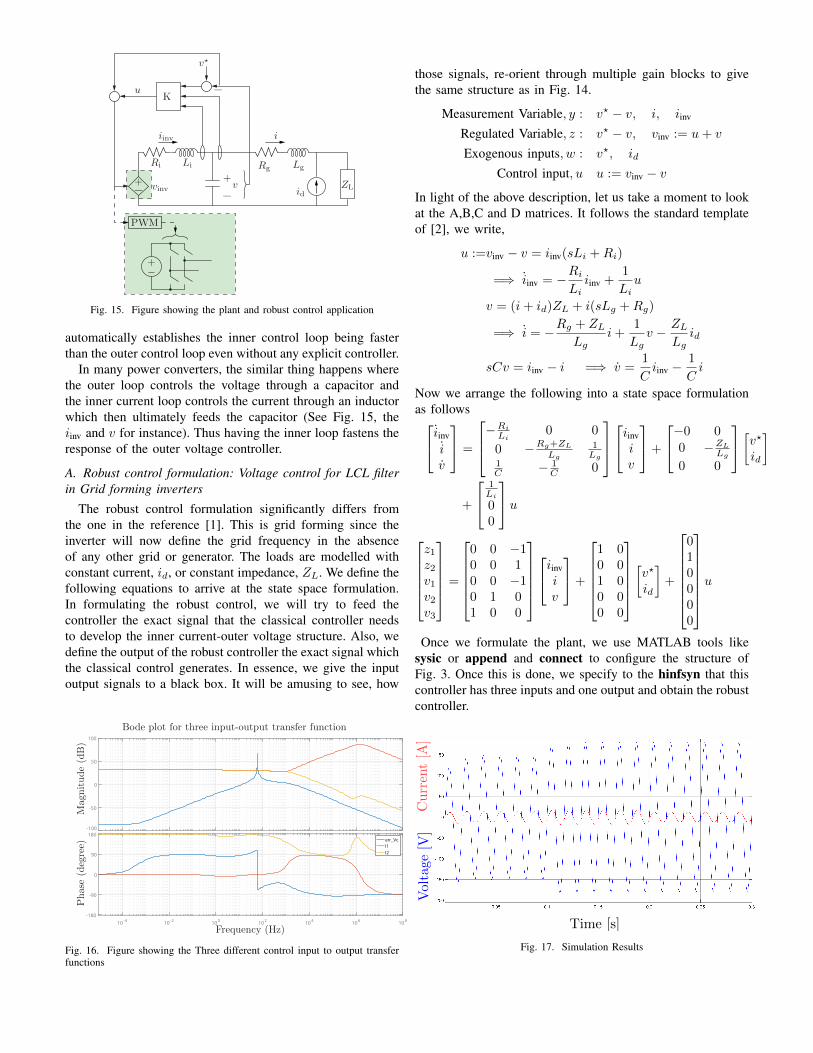
Fig. 15. Figure showing the plant and robust control application

automatically establishes the inner control loop being fasterthan the outer control loop even without any explicit controller.

In many power converters, the similar thing happens wherethe outer loop controls the voltage through a capacitor andthe inner current loop controls the current through an inductorwhich then ultimately feeds the capacitor (See Fig. 15, theiinv and v for instance). Thus having the inner loop fastens theresponse of the outer voltage controller.

A. Robust control formulation: Voltage control for LCL filterin Grid forming inverters

The robust control formulation significantly differs fromthe one in the reference [1]. This is grid forming since theinverter will now define the grid frequency in the absenceof any other grid or generator. The loads are modelled withconstant current, id, or constant impedance, ZL. We define thefollowing equations to arrive at the state space formulation.In formulating the robust control, we will try to feed thecontroller the exact signal that the classical controller needsto develop the inner current-outer voltage structure. Also, wedefine the output of the robust controller the exact signal whichthe classical control generates. In essence, we give the inputoutput signals to a black box. It will be amusing to see, how

-100

-50

0

50

100

10-4 10-2 100 102 104 106 108-180

-90

0

90

180err_VcI1I2

Mag

nitude

(dB

)P

has

e(d

egre

e)

Frequency (Hz)

Bode plot for three input-output transfer function

Fig. 16. Figure showing the Three different control input to output transferfunctions

those signals, re-orient through multiple gain blocks to givethe same structure as in Fig. 14.

Measurement Variable, y : v? − v, i, iinv

Regulated Variable, z : v? − v, vinv := u+ v

Exogenous inputs, w : v?, id

Control input, u u := vinv − vIn light of the above description, let us take a moment to lookat the A,B,C and D matrices. It follows the standard templateof [2], we write,

u :=vinv − v = iinv(sLi +Ri)

=⇒ i̇inv = −Ri

Liiinv +

1

Liu

v = (i+ id)ZL + i(sLg +Rg)

=⇒ i̇ = −Rg + ZL

Lgi+

1

Lgv − ZL

Lgid

sCv = iinv − i =⇒ v̇ =1

Ciinv −

1

Ci

Now we arrange the following into a state space formulationas followsi̇inv

i̇v̇

=

−Ri

Li0 0

0 −Rg+ZL

Lg

1Lg

1C − 1

C 0

iinviv

+

−0 00 −ZL

Lg

0 0

[v?id

]

+

1Li

00

uz1z2v1v2v3

=

0 0 −10 0 10 0 −10 1 01 0 0

iinviv

+

1 00 01 00 00 0

[v?

id

]+

010000

uOnce we formulate the plant, we use MATLAB tools like

sysic or append and connect to configure the structure ofFig. 3. Once this is done, we specify to the hinfsyn that thiscontroller has three inputs and one output and obtain the robustcontroller.

Time [s]

Vol

tage

[V]

Curr

ent

[A]

Fig. 17. Simulation Results

-300

-200

-100

0

100

10 -4 10 -2 10 0 10 2 10 4 10 6 10 8-270

-180

-90

0

90Inner CurrentOuter Voltage

Magn

itude

(dB

)P

hase

(deg

ree)

Open Loop Transfer Function Bode Plot

Frequency (Hz)Fig. 18. Figure showing the different open loop plots

TABLE ISIMULATION: STEPS OF OPERATION

Time Interval v? id

0-0.1 s 150 V 0 A0.1-0.2 s 180 V 0 A0.2-0.5 s 180 V 5 A

B. Comparison to classical control structure

To bring a one-to-one comparison with the classical ICOVstructure, let us now compare from the Fig. 14 and write thefollowing equations,

u := vinv − v = Ki(i?inv − iinv)

= Ki(Kvev + i− iinv)

= Ki

(Kv(v

? − v) + i− iinv

)= KiKv(v

? − v) +Ki(i− iinv)

Comparing the equation above to the Robust control basedH∞ controller we get, the following

u := vinv − v = K1(v? − v) +K2i+K3iinv

And this is the most remarkable trait that we obtain fromthe results (Fig. 16) that K2 and K3, are almost exactly thesame in the bandwidth of concern except that K3 has a phaseexactly 180◦ out of that of K2. This means, K2 = −K3.This is also immediately apparent from the equationu = KiKv(v

? − v) +Ki(i− iinv), that Ki = K2 = −K3.

The following are the simulation results as shown in Fig.17. We perform the following test on the model to check thereference tracking and disturbance rejection.

The following are the observations from Fig. 17

• The reference tracking is within two cycles. This is fastenough. There is no overshoot which means that thecontroller has high damping. The current injection startsat 0.2s. However, there is no appreciable change in thevoltage.

-200

-150

-100

-50

0

10 -2 10 0 10 2 10 4 10 6 10 8-270

-180

-90

0

90Inner CurrentOuter Voltage

Mag

nitude

(dB

)P

has

e(d

egre

e)

Closed Loop Transfer Function Bode Plot

Frequency (Hz)

Fig. 19. Figure showing the closed loop plots

• The net current flowing through the inverter grid sidecurrent now reduces by 5A since that is supplied by thedisturbance current.

C. Relationship between bandwidths

This is a very important topic and probably one of thekey motivation behind the project. In classical control thebandwidth relation between the inner and outer loop is alwaysby a factor of ten since we know that the phase contribution ofa pole or zero is negligible below a factor of ten. Thus wheninner loop bandwidth is ten times faster, we ignore the designof inner loop in the outer loop and assume that the inner loopTF is basically unity in the frequency range of interest of theouter loop.

This is the reason for this exercise, we try to plot the innerand the outer loop.

Inner Loop Gain := `i(s) = K2(s)1

sLi +Ri= Ki(s)

1

sLi +Ri

Outer Loop Gain := `v(s) =K1(s)

K2(s)

1

sC= Kv(s)

1

sC

Fig. 18 shows the loop gains of the two transfer functions.

10-2 100 102 104 106-140

-120

-100

-80

-60

-40

-20

0

20Inner CurrentOuter Voltage

Mag

nitude

(dB

)

Frequency (Hz)

Closed Loop Transfer Function

Fig. 20. Figure showing the closed loop plots for Case I

TABLE IIDIFFERENT WEIGHTING FUNCTIONS AND ITS EFFECT ON THE CLOSED LOOP BANDWIDTH RATIO AND FEASIBILITY OF SIMULATION

Case Ws Wu Wd ωi/ωv Simulation Works? γ

I 50s/1e3+1

s2+2ωr+ω2r

s2+0.001 2ωr+ω2r

s2+2ωLC+ω2LC

s2+2 10ωLC+ω2LC

1 1 ≈ 10−2 NO (Fig. 20,22) 6.2828

II 50s/1e3+1

s2+2ωr+ω2r

s2+0.001 2ωr+ω2r

s2+2ωLC+ω2LC

s2+2 10ωLC+ω2LC

0.01s/100+1

s/106+11 ≈ 1 NO (Fig. 21) 4.9437

III 50s/1e3+1

s2+2ωr+ω2r

s2+0.001 2ωr+ω2r

s2+2ωLC+ω2LC

s2+2 10ωLC+ω2LC

1 1s/3147+1

≈ 103 YES 4.566

IV 50s/1e3+1

s2+2ωr+ω2r

s2+0.001 2ωr+ω2r

s2+2ωLC+ω2LC

s2+2 10ωLC+ω2LC

0.01s/100+1

s/106+11

s/3147+1≈ 103 YES (Fig. 17,19) 2.395

Whereas, Fig. 19 shows the closed loop TF which is basically`i/(1 + `i) and `v/(1 + `v) respectively. We define thebandwidths to be ωi and ωv respectively.

Fig. 19 shows that the bandwidth of these two loops isseparated by a factor greater than the rule of thumb or 10.

The following questions are important.

� How does the bandwidth of the generated controllersrelate to the weighting functions.

� How does the bandwidth of the generated controllersrelate to the value of γ.

� How does the controller actually does the trick to generatethe ICOV structure. What is the ARE/LMI or weightingfunction that is forcing to do this.

We have not been able to come to any direct conclusionor a good understanding of these questions, but the followingpoints might help.

D. Observations from the Table II

We can make some observations from the different weight-ing functions. First and foremost is that we do need the threeweighting functions to be specified. If we do not specify them,we get unstable controller. It also, very intuitively gives us theconclusion that the plant is stabilized only when the innercontrol loop is faster than the outer one. We knew this. Theonly thing we wanted to find was, how much faster?

These are some interesting conclusions

100 101 102 103 104 105 106-140

-120

-100

-80

-60

-40

-20

0

20Inner CurrentOuter Voltage

Mag

nitude

(dB

)

Frequency (Hz)

Closed Loop Transfer Function

Fig. 21. Figure showing the closed loop plots for Case II

Vol

tage

[V]C

urr

ent

[A]

Time [s]

Fig. 22. Figure showing the response of the plant to the same kind of referenceas we had subjected in Table I

• We are often accustomed to having resonant controllerin both the inner and the outer controller. Fig. 18 showsthat the inner controller can as well only be a proportionalcontroller. This technique has well been used in literatureperhaps in an ad-hoc way. The general norm is, if theouter loop takes care of steady state error by integratoror resonant controller, the inner loop might not as wellhave that. We come to the same point, only through robustcontrol techniques.

• We observe that the weighting function Ws very stronglyties to the error in voltage reference. We can thus claimthat the zero crossing of the weighting function influencesthe bandwidth of the closed loop bandwidth of the outervoltage controller (`v).

• The question then remains, is to see that what deter-mines the current loop bandwidth. We observe that theweighting function Wd related to the disturbance incurrent. Thus it might be true that changing the weightingfunction, Wd might change the variable current controllerbandwidth. The present Wd is, 1

s/3147+1 . This signifiesthat all the disturbances upto the frequency 10 timeshigher than maximum disturbance will be tried to berejected. Thereafter, to reduce sensitivity to noise, weneed to roll-off Wd. The minimum we can reduce this isto slightly higher than 2π 60 = 377rad/s. This Wd stillgives a ratio of ωi/ωv to be very high, typically in orderof 104. Only when we reduce the pole of Wd significantlylow, to be around the following Wd, 1

s/10−4+1 do weget to a point where the ratio of ωi/ωv is much lower,

around 10−2. Now when we simulate the plant with thiscontroller, we get an oscillatory and unstable system.

V. CONCLUSION AND SCOPE FOR IMPROVEMENT

In this paper we have demonstrated the use of the weightingfunction in synthesizing controllers for the power convertersfor various filter and signals (ac and dc). We have discussedthe design and selection of these weighting functions andshown their performance over classical controller with cogentsimulations. Finally we took up the interesting problem toshow how a complicated intuition-based classical controllerstructure comes from the rigorous mathematics of the robustcontrollers. Through various test cases, we show that thebandwidth ratio can only be pushed to around 103, muchhigher than what was already known from the classical control.

The main drawback of this current work is not having aclear understanding of the clear ties between the weightingfunctions and the controller synthesis when there are multipleweighting functions and we are dealing with a MIMO system.

If we had a better mathematical model, we could have obtainedsome valuable information from the γ and commented upona theoretical minima on the ωi/ωv ratio.

REFERENCES

[1] B. Johnson, S. M. Salapaka, B. Lundstrom, and M. V. Salapaka, “Optimalstructures for voltage controllers in inverters,” 2015.

[2] P. F. Dullerud G. E., A course in robust control theory – a convexapproach. Springer, 2013.

[3] G. K. Zhou K., Doyle J.C., Robust and optimal control. Prentice Hall,1996.

[4] S. Skogestad and I. Postlethwaite, Multivariable Feedback Control. JohnWiley and Sons, 2010.

[5] S. S. Braatz R., Morari M., “Loop shaping for robust peformance,”International Journal of Robust and Nonlinear Control, vol. 6, pp. 805–823, 1996.

[6] T. A. Doyle J., Francis B., Feedback Control Theory. Wiley, 2nd ed.,2008.

[7] D. Holmes and T. Lipo, Pulse Width Modulation for Power Converters:Principles and Practice. Wiley-Interscience, 2003.

[8] P. Channegowda and V. John, “Filter optimization for grid interactivevoltage source inverters,” IEEE Transactions on Industrial Electronics,vol. 57, pp. 4106–4114, Dec 2010.