CALCULATION OF THE ABERRATION SPOT - IMPROVED NUMERICAL ALGORITHM

Marek LEWKOWICZ∗, Jerzy NOWAK, Marek ZAJĄC

Institute of Physics, Technical University of Wrocław Wyspianskiego 27, PL 50-370 Wrocław, Poland ∗Mathematical Institute, Wrocław University

key terms: aberrations, point spread function, numerical methods

Lewkowicz, Nowak, Zaj¹c "Calculation of the aberration spot...", p. 2

ABSTRACT

In the paper a numerical algorithm for calculation of the point spread function from the complex light amplitude known on the output pupil of the imaging system is described. First step of this algorithm includes a global polynomial approximation of the input data given in a number of points distributed arbitrarily over the entire output pupil. In the next step the numerical calculation of the diffraction integral is performed. After transition to the polar co-ordinates and dividing the region of integration into a number of infinitesimal subregions of square shape the exponent in the integrand is approximated locally by a polynomial and then the whole integrand is approximated by a polynomial multiplied by the exponential function with linear exponent. Finally the respective integration is performed analytically. The analysis of the accuracy obtained as well as the results of exemplary calculations prove that the described algorithm is very useful in the analysis of image quality of such imaging elements as hybrid (diffractive-refractive) lenses.

Lewkowicz, Nowak, Zaj¹c "Calculation of the aberration spot...", p. 3

1. PROBLEM

One of the most important problems occuring in optical design is related to the evaluation of imaging quality. Standard methods include typically calculation of Seidel aberration coefficients of the third or higher orders, wave aberration, aberration spot and optical transfer function. The mentioned characteristics are usually estimated numerically. Standard numerical programmes, including commercially available, most frequently employ typical ray-tracing procedures to this aim. For instance the aberration spot shape and dimensions are concluded from the spot-diagram. However the geometrical methods have only limited value, especially when the investigated optical element has small aberrations [1]. Geometrical method of aberration spot estimation does not include the influence of diffraction, which becomes to prevaile in well-corrected optical systems. Therefore it seems that the method of aberration spot calculation based on the diffraction integral might be very useful. Assuming that the complex light amplitude ( )ηξ,U (light wavefront) is known in the output pupil of the optical system of interest (see Fig. 1), the light amplitude in the detection plane ( )y,xU distant by the value z can be calculated from the diffraction integral that can be written in the form

( ) ( ) { }ΣΛηξ⋅= ∫∫

Σ

dRikRexp,UCy,xU (1)

where C is complex constant, R is a distance from point ( )ηξ, to ( )y,x , Λ is a directional coefficient and Σ is the output pupil area. In many applications, including the analysis of imaging quality of the diffractive optical elements the aperture angle as well as the field angle are relatively small. Therefore the diffraction integral (1) can be simplified to the form ( ) ( ) { } Σηξ⋅= ∫∫

Σ

dikRexp,U©Cy,xU (2)

If we assume that the spherical wave emerging from the object point is transformed by the imaging optical system into the image wave, then the complex light amplitude in the output pupil of this system is ( ) { }Φ=ηξ iexpA,U . Its transformation ( )y,xU described by the integral (2) describes the complex point spread function. Its square is the intensity point spread function ( )y,xH

( ) ( ) { }2

dikRexp,Uy,xH Σηξ≈ ∫∫Σ

(3)

The point spread function is typically calculated in the image plane, to which a wave ( ) { }Φ=ηξ iexpA,U emerging from the oputput pupil converges. Therefore, using the

concept of Gauss reference sphere R0 and wave aberration W, the expression (3) can be written in the form

Lewkowicz, Nowak, Zaj¹c "Calculation of the aberration spot...", p. 4

( ) { } { } ( ){ }2

0

2

dWRRikexpAdikRexpiexpAy,xH Σ+−=ΣΦ≈ ∫∫∫∫ΣΣ

(4)

where the amplitude A in the output pupil is commonly assumed to be equal to 1. In their former papers [2, 3] the authors of this paper had used a simple algorithm for numerical evaluation of this integral based on the Gauss integration method. Such approach seemed to give satisfactory results in the evaluation of the imaging quality of holographic lenses [4 - 7]. However while analysing more complex optical imaging elements, such as hybrid (diffractive-refractive) lenses, this method appeared to give unreliable results. The reason was that the integrand in the equation (4) is a rapidly oscillating function. More accurate algorithms for numerical calculation of the diffraction integral are known in the literature. Several methods for computing the diffraction integrals are presented in [8] One of them is approximating the kernel of the integral in such a way thet the integral takes on the form of the Fourier transform (Fraunhofer approximation, see [9]); then algorithms for Fast Fourier Transformation (FFT) can be applied (see [10]). Another group of methods relies on approximating the integrand so that the integral could be evaluated analytically or with mixed analytic and numerical methods. In case of linear approximation to the exponent the integral can be expressed analytically through elementary functions. Higher accuracy can be obtained by second order (parabolic) approximation to the exponent. A method developed in [8] is a fast algorithm for computing one-dimensional diffraction integrals with parabolic exponent. The values obtained with this method are used as input data for another integration in the second direction. That integration is performed with the help of the standard Gauss-Legendre method. Our approach differs from the above as we use higher order approximation to the exponent in both variables; we then replace trigonometric functions applied to non-linear components of the approximation by their Taylor expansions. The resulting functions are products of polynomials by sine or cosine functions applied to linear functions and can be evaluated analytically.

2. DESCRIPTION OF THE ALGORITHM In this section we describe the technicalities of our algorithm for computing the diffraction integral (4). We also present some results of symbolic and numerical computations that suggest what level of accuracy of the algorithm one could expect. We think there are two interesting points of our approach. One is the way we transform the empirically given discrete data into a mathematically correct problem with data being a continuous (in fact polynomial) function. The other is a high-order local approximation of the integrand, which leads to analytically integrable functions. Both questions are discussed in detail below.

2.1. Numerical difficulties in computing oscillating integrals

The diffraction integral (4) is a two-dimensional version of an oscillating integral of the form ( ) ( )dxexg xif∫ (5)

Lewkowicz, Nowak, Zaj¹c "Calculation of the aberration spot...", p. 5

where f is a real and g a possibly complex function of n-dimensional variable x. Its characteristic feature is rapid oscillation of the integrand: even for relatively regular function f, which can be well approximated with linear functions, the real and imaginary parts of ( )xife , that is ( ))x(fcos and ( ))x(fsin , vary rapidly. The number of oscillations depends on the size of the image of the function f and exceeds sup( ) inf ( ) /f f− 2π . If we use standard, universal methods of integration, numerous oscillations together with accuracy requirements force one to use grids with many nodes, which leads to long computing time.

2.2. Error estimation. Many numerical integration procedures depend on a parameter like the number of nodes or the degree of the approximating polynomial (as in our algorith described below). Increasing the parameter gives better accuracy of the result but lengthens the time needed for the calculations. The accuracy of the result is commonly estimated by assuming that decimal digits stable under increasing of the parameter are exact. While this approach works perfectly in most situations it may be misleading in special badly conditioned cases since the stabilizing process may be extremely slow or discontinuous: the seemingly stabilized result may eventually change or jump to another after the parameter exceeds some critical value. Our search for a new algorithm stems from the fact that the results obtained by simple, fast algorithms seemed unreliable in some special cases and we needed an independent way of estimating the accuracy of the results. All the algorithms that we considered adhere to the following pattern. The domain of integration is divided into sub-domains, the integrand is approximated in each subdomain, and various integration procedures are applied to the approximating function. The place critical for accuracy is typically the approximation of the integrand in the subdomain since the type of the approximating function is chosen so that the integration procedures applied to it could be highly accurate. Therefore we adopt the folowing measure of accuracy of the algorithm. In each subdomain we measure the difference between the integrand and its approximation in several random points and we assume that the discrepancy of the two functions in whole subdomain does not exceed the maximum of those numbers. The sum of those local errors multiplied by the size of each subdomain gives an upper bound for the error of the result. We call it the estimated accuracy of the result in contrast to the actual accuracy i.e. the difference between the obtained result and its exact (usually unknown) value. In a series of computations the above mentioned measure of estimated accuracy was applied to several integration algorithms including those using different linear approximations to the integrand (methods 0-3), linear aproximation to the exponent (method 4) and our algorithm with different degrees of the approximating polynomial. The calculations were performed for the following sample situation. We consider an imaging system with a circular output pupil Σ of radius r=5.0 mmm. It produces a non-aberrated spherical wave front focused at the point ( )2z,0,0S = , z2 100= mm. Let the wavelength be λ = 0 0006. mm. The phase function for this wave is ( ) ( )ηξ−=ηξΦ ,kR, 0 (6)

Lewkowicz, Nowak, Zaj¹c "Calculation of the aberration spot...", p. 6

where ( )ηξ,R 0 is the distance from ( )0,,ηξ to ( )2z,0,0 The diffraction integral (4) for the point P x y z( , , ) takes on the form ( ) ( ){ } ηξηξ= ∫∫ dd,ifexpz,y,xU (7) where ( ) ( ) ( )[ ]ηξ−ηξ=ηξ ,,z,0,0R,,z,y,xRk,f 2 . Here R x y z, , , ,ξ η is the distance form ( , , )x y z to ( , , )ξ η 0 . The results of calculations for the non-aberrated phase are shown in Figure ... Each point in the table represents one example of calculations. <Opisac w zaleznosci od wykresu> The horizontal coordinate (values 0..5) denotes logarithm of time in hundredths of seconds (0=0.01s, 1=0.1s, 2=1s,..., 5=1000s). The vertical coordinate (values -1..10) is the number of exact decimal digits guaranteed by the method. In Fig... we show the results for the case where an aberration represented by a component 40\ksi\eta was added to the phase (6). The results show that it is practically impossible to ensure accuracy of 3 decimal places with methods 0-3. Method 4 is much better but practically works up to 5 decimal digits. With our method we are able to obtain 8-9 exact digits. The fundamental difference in the algorithms that enables this is the fact that for higher degrees of the polynomials increasing the number of nodes has much stronger impact on the accuracy than in the case of linear approximations. It should be noted that in most cases the actual accuracy is much better than the estimated one, but only evaluating the latter makes it possible to find highly accurate results and thus to estimate the former. The complex machinery developed in our algorithm results in a relatively long computational time in comparison with simple methods for the same number of nodes. In many cases, when high accuracy is not required, those methods may work faster. Therefore a typical application of our algorithm is as follows. We use it for computing the results for several random points with high estimated accuracy. In this way we obtain reliable numerical results. They serve for testing the actual accuracy of some simpler methods and the best of them can be used for computations in all needed points.

2.3. Approximating discrete data with polynomials It is quite common in numerical problems involving integration that the integrated function is given by values in a number of separate points. We assume that the phase function Φ is numerically represented by a collection of triples ( , , )x yi i iφ , where φi is interpreted as the value of the phase function at the point ( , )x yi i . We do not assume that the points ( , )x yi i form a regular grid in any special co-ordinate system, as Cartesian or polar. Nevertheless we do expect that the points do not show any extreme irregularity. For example we do not accept data all lying on one side of a straight line halving the domain. A precise mathematical formulation of the integration problem requires the integrand to be defined at all points of its domain. We therefore need to choose a way to interpolate our discrete data with a continuous function. In standard integration problems there is little difference in the numerical result between linear, quadratic or any other kind of interpolation. The choice of the interpolation method has impact on efficiency of the algorithm rather than the value of integral. Quite opposite, if the

Lewkowicz, Nowak, Zaj¹c "Calculation of the aberration spot...", p. 7

integrand is an oscillating function, the integration involves numerous cancellations, and the final result depends strongly on the way the cancellations are performed. It is threfore crucial to make a correct choice of the function we accept to interpolate our data. If our initial data were given in a regular grid we probably would be tempted to choose a linear or quadratic approximation as our favourite integrand. The interpolation would be local in the sense that a separate linear (or quadratic) function would be chosen for each subrectangle of the grid. In the absence of a regular grid a possible approach could be to triangulate the domain in such a way that the given points ( , )x yi i become the vertices of the triangulation. As the interpolating function we could choose then the only extension of the values φi (given for the vertices) to the function linear on the simplices of the triangulation. The triangulation problem has no natural unique solution. It would require a separate algorithm to find and automatically choose one of possible existing triangulations. For these reasons we prefer to adopt the following approach. We approximate our data with a polynomial in variables x,y in such a way that the sum of squares of errors (i.e. defferences between the values of our polynomial and the prescribed data φi ) is the least possible. We apply a full real-valued polynomial of degree n of the form ( ) ∑

≤+≤

=nji0

jij,i yxay,xQ (10)

The coefficients of the polynomial minimizing the sum of squares of errors in the class of polynomials of fixed degree n are uniquely determined and can be computed with any standard method of least-square approximation. We treat the integral in 3 steps described below 1. pass to polar coordinates and replace ( )),(fcos ηξ with ( )),(Tcos ηξρ , T -

a polynomial; 2. write T as L+Q where L is a lineal and Q contains terms of degree higher or equal 2; 3. replace ( )),(Qcos ηξ and ( )),(Qsin ηξ by its Taylor expansion in 2 variables 4. reduce the problem to the single integrals of x bxn sin( ) and x bxn cos( ) and compute

them by parts or by Taylor expansion, depending on the values of the parameter b. We illustrate our approach in the case of the non aberrated phase function of a wave converging to (0,0,100), that is the analytic function f x y x y( , ) = − + + −2 2 2100 100. We compute the phase function in 386 random points ( , )x yi i and we approximate these values with a polynomial of degree 2, 3, 4, 5 and 6. The phase function varies in the range [0.0,1308.18]. In the Table 2 we give the degree of approximating polynomial Pn , the maximum deviation (i.e. the difference P x y f x yn i i i i( , ) ( , )− ) and the maximum difference between coefficients of polynomial Pn and and the maximum of corresponding coefficients in Taylor series for f. We see that raising the degree of the approximating polynomial from even number by one (e.g. from 2 to 3 or from 4 to 5) does not improve the approximation. This is explained by the fact that the phase function is obtained with squares and square roots, its Taylor series contain only even powers of x and y, and therefore it is well approximated by even degree polynomials. In fact in our example the maximum error even increased slightly when passing from degree 4 to 5; this is possible since we

Lewkowicz, Nowak, Zaj¹c "Calculation of the aberration spot...", p. 8

minimise the l2 -norm of the error (sum of squares), not tne l∞ -norm (the maximum of its absolute value). A physical justification for this approach is offered by the fact that a commonly adopted measure of aberration of an optical instrument are coefficients of a polynomial approximation of the difference between the phase function and a spherical function. This approach implies that a physically instructive representation of a phase should be a polynomial of even degree between 4 and 8. Although we are not going to globally (that is in the whole domain) approximate the function kR with a polynomial with the purpose of integrating it, it may be of interest to see the quality of such approximation for a sample point x2 0 03= . . In the Table 3 we have the maximum error of Φ+ kR , in dependency on the polynomial degree. In opposition to the previous example we see that the function is better approximated with odd-degree polynomials. This can be explained by observing that in the absence of aberration Φ equals −kRo , R is a translation of R0 which is of series in x y2 2+ .

( )0RRkkR −=+Φ behaves similarly to ( ) n2n2 xhx −+ and should be approximated with odd degree polynomial.

2.4. Oscillating integrals with polynomial exponents

Approximating the discretely defined phase data with a polynomial described above transforms diffraction integral into a well posed mathematical problem, which reads as follows: integrate ( ) ηξηξ dd),(fcos in a disk, with f ( , )ξ η being a polynomial of degree ≤10. Here and in the sequel cosine may be replaced by sine. We pass to polar coordinates with the domain 0 0≤ ≤ρ r , 0 2≤ ≤θ π . We divide the domain into n nρ θ⋅ regular rectangles and confine ourselves to calculate the integral over one of those small rectangles. Let ρ θ0 0, denote the centre of the rectangle. We expand the polynomial f ( , )ξ η (given in Cartesian coordinates) in its Taylor series T ( , )ρ θ in polar coordinates ρ θ, centered in ρ θ0 0, . We expect to use the expansion up to tenth order. We want to estimate the error introduced by passing from ( )),(fcos ηξ to

( )),(Tcos θρ . Therefore we consider the example introduced in section 2.1 and we compute the difference between the value of T at the vertex v of small rectangle and the actual value f v( ) of the polynomial itself at the vertex v. In the Table 4 we show the maximum error for the 10 by 10 partition of the domain (n nρ θ= = 10), for different degrees of the Taylor polynomial varying from 0 to 4. The results are given for the phase function Φ and for the exponent Φ+ kR , each approximated locally (that is over the small rectangle, with origin at its centre) by a polynomial of degree at most 4: We see that when the degree of the approximating polynomial is growing the error tends to zero quite fast. Note that in order to improve accuracy at this step we can handle two independent parameters: the number of nodes n nρ θ⋅ and the degree of opproximation polynomial Deg. If we multiply the number of nodes ( , )n nρ θ in each direction by a factor of n, then the computation time enlarges n2 times, while error decreases nDeg+1 times. This is seen in the Table 5, computed for n nρ θ= = 10 20 40, , , all for Deg = 4 . We see that

the error decreases by a factor of around 2 325 = in each step.

Lewkowicz, Nowak, Zaj¹c "Calculation of the aberration spot...", p. 9

The optimum choice of n nρ θ, and Deg for given accuracy is not clear. Higher degree Deg speeds up the convergence when the number of nodes increases. On the other hand it lengtens the time for fixed number of nodes. At this step we can sum up the above calculations by saying that the integrand can be satisfatorily approximated by

( )),(Tcos θρ , where T is a polynomial in ρ θ, . As the second step we decompose T as T a b c Q= + + +ρ θ ρ θ( , ) (11) where a b c+ +ρ θ is the linear part of T, and Q( , )ρ θ is a polynomial with homogeneous components of degree two or higher. Thus ( )),(Tcos θρ equals a sum of two expressions of the form ( ) ( )),(Qcsncbacsn 21 θρ⋅θ+ρ+ , where csn1 and csn2 denote cosine or sine. The integral is to be computed in a rectangular neibourhood of ( , )0 0 . Therefore we expand ( )Qcsn 2 in its Taylor series in two variables around (0,0) and take its components of degree of Q. Thus we and obtain integrands ( ) ( )θρ⋅θ+ρ+ ,Pcbacsn1 with P - a polynomial, deg( ) deg( )P Q= . The crucial point here is the error introduced by passing from ( )Qcsn 2 to P. The Taylor expansion gives good accuracy only for small x (that is Q( , )ρ θ in our notation). This requires that Q, which is equal to the error of the linear approximation of Φ+ kR be small. The error for different numbers of nodes and Deg = 4 are shown in the Table 6 We see that we get error less than 1.0E-1 for linear approximation with 20 by 20 nodes. The final step is integrating ( ) ),(Pcbacsn1 θρ⋅θ+ρ+ with P - a polynomial. This is reduced to single integrals of x bxn cos( ) and x bxn sin( ), n = 0,1,2,... These integrals can be computed by expanding cos( )bx and cos( )bx in their Taylor series for small b or by integration by parts for large b.

3. ALGORITHM ACCURACY

In order to test the developed algorithm several calculations were performed. In the first test we wanted to check the accuracy of the obtained results in dependency on the number of integration points. Three sets of input data were selected as described below. First one, referred as "test #1" represented perfectly spherical wavefront converging to the point located on axis in the distance z mmi = 100 . The radius of the output pupil was set to r mm= 10 , what corresponds to the F-number equal to 1:5. The second set of input data ("test #2") was generated as the spherical wavefront converging to the object points having coordinates z mmi = 200 , x mmi = 2 , hovewer affected by Seidel aberrations characterized by the following coefficients: S = ⋅3 105, Cx = − ⋅3 105, A x = ⋅6 105, Dx = − ⋅6 105, F = ⋅9 105. The output pupil radius was r mm= 2 , thus the relative F number was equal to 1:50. The last set of data ("test #3") was obtained by numerical calculation of the wavefront in the output pupil of a hybrid focusing lens. This lens was a diffractive-refractive doublet with the following construction parameters. Radii of curvature of the glass substrate: R mm1 56 989= . , R mm2 1576 0= − . . Lens thickness: d mm= 3 . Index of refraction of the lens material: n = 1 5. . Diffractive microstructure deposited on the second surface is generated by two spherical wavefronts of radii: R mmα = −37 317. , R mmβ = −36 093. while the light wavelength equals to λ = 632 8. nm. The lens has

Lewkowicz, Nowak, Zaj¹c "Calculation of the aberration spot...", p. 10

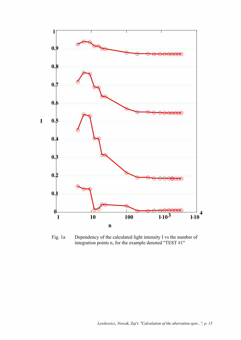
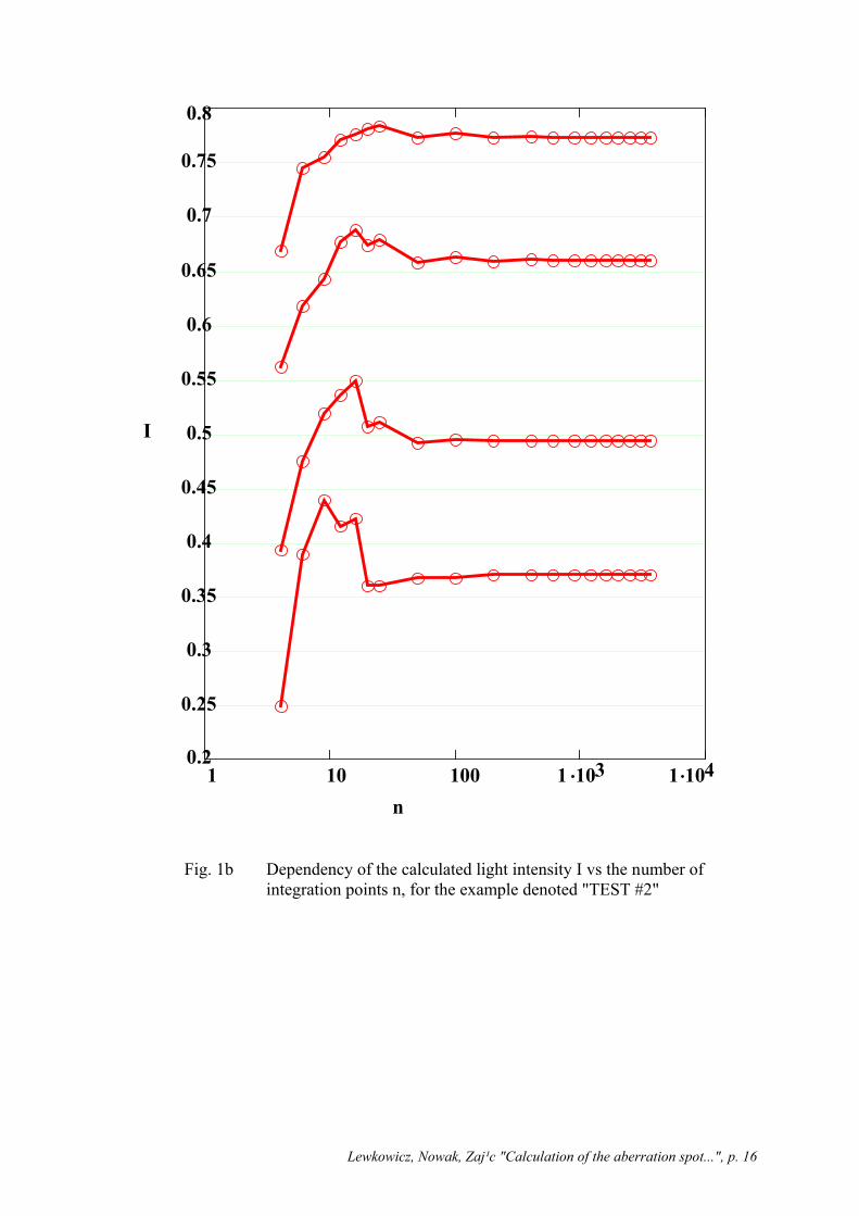
focal length f mm= 100 and relative aperture 1:10. Paralell light beam falling under the field angle ω = 0 03. was converging to the focal plane, however the best image plane was established to be shifted by about 0.75 mm outwards. For the described three cases the light intensity in the aberration spot was calculated in selected points along the cross-section of the aberration spot. The results are presented in the Figs. 2a, 2b, 2c, respectively, as the dependency of the calculated intensity versus number of integration points. It can be easily seen, that the results became stable starting from about 103points of integration. For the lens of small aperture (test #2) this number is substantially slower, what suggests, that not the overall number of points is important, but rather their density over the output pupil. While the imaging qulity of hybrid lens is to be evaluated in the first step the wavefront in the output pupil of the investigated imaging element has to be calculated by comparing the optical path length along a number of rays traced from the object point through the optical system. The rays are uniformly distributed over the input plane of the system, but due its aberrations their distribution over the output plane is changed. It is not possible then to obtain the phase data directly in the regular grid (e.g. rectangular) as it is necessary for the integration algorithm. Therefore it was necessary to initially approximate the phase distribution over the output pupil. The two-dimensional polynomial with respect to variables x and y of order n was choosen to this aim. Its form is similar to Seidel expansion. The test was performed to check the dependency of the calculated light intensity on the order of this polynomial. The exemplary results of two cases are presented in the Figures 3a, 3b. Both present the dependency of the light intensity calculated in selected points in the aberration spot obtained with the same hybrid lens as used in the test #3. The relative apperture was kept equal 1:10 in the first case, and increased to 1:4 in the second case. The same number of integrating points (equal 104) was used. The aberration spots were calculated in the best image planes z mmi = 100 75, , and z mmi = 100 60. respectively. From the presented results it is seen, that if the relalative aperture is relatively small (Fig. 3a) polynomial of the fifth order is enough. If the imaging element has greater aperture than higher order aberrations became also important, but approximation with the polynomial of the 6-th order gives satisfactory results. For the typical applications the approximation of the phase function with the fifth order polynomial and taking the number of integration points over the output pupil of the order 103 leads to the values of the light intensity in the image plane calculated with an error substantially less that 0.1%, what in the authors opinion, is fairly satisfying. If the PC computer with Pentium processor and 100MHz clock is used calculation of the light intensity in one object point takes ca. 0.12s.

3. EXAMPLES OF APPLICATION To illustrate the practical use of the described method we performed the analysis of imaging quality of the hybrid (diffractive-refractive) lens according to the construction parameters described in the previous paragraph (lens #3). Wave aberration in the input pupil of this lens was calculated from the difference of the optical path along a given ray and the principal ray. Rays are equally spaced over the input pupil, however due to aberrations the distribution of the points of their intersection with the output pupil plane

Lewkowicz, Nowak, Zaj¹c "Calculation of the aberration spot...", p. 11

was disturbed. Then the light intensity distribution in the aberration spot was calculated. the obtained results were presented in the following figures. In the Fig. 4 the wave aberration and aberration spots for the hybrid lens of relative aperture equal 1:10 and two object field angles equal 0 and 0.03 respectively are presented. The polynomial of 5-th order was used. Number of integration points was 60*60. The investigated lens has relatively small aberrations (spherical aberration and coma are corrected, see [11]). For the object on axis wave aberration does not exceed λ and the aberration spot does not differ substantially from the aberration free one. For the object point off axis the influence of non-corrected field aberationcan be noticed. In the Fig. 5 the light intensity distribution in central point of the aberration spot for field angle equal to zero is calculated along the z axis. A relatively small depth of focus, not exceeding 1 mm is seen, what is in accordance with expectations. the Fig. 6 presents the wave aberration spots for the same hybrid lens, but of greater aperture (relative aperture is 1:4). The calculations are made for the field angle equal to zero. It is seen, that higher order aberrations cause the worsening of the image. Maximum wave aberration is almost 6λ

4. ACKNOWLEDGMENTS

5. REFERENCES 1. M. Zając, J. Nowak, "Holographic optical elements used in spectroscopy: some

remarks on image quality", Appl. Optics, vol. 29, no. 34, (1990), 5198 - 5202. 2. J. Nowak, M. Zając, "Numerical method for the calculation of the light intensity

distribution in the holographic image", Opt. Appl, vol. 12, no. 3-4 (1982), 353 - 361.

3. J. Nowak, M. Zając, "Investigations of the influence of hologram aberrations on the light intensity distribution in the image plane", Optica Acta, vol. 30, no. 12 (1983), 1749 - 1767

4. J. Nowak, M. Zając, "Numerical investigations of the imaging by holographic lens", Optik, vol. 70, no. 4 (1985), 143 - 145.

5. M. Zając, J. Nowak, "Collimating holographic lens on curved surface - a numerical study", Optik, vol. 80, no. 4 (1987), 137 - 140

6. M. Zając, J. Nowak, A. Gadomski, "Hologeraphic lens - study of imaging quality", Opt. Appl, vol. 19, no. 2 (1989), 229 - 244.

7. B. Dubik, J. Masajada, J. Nowak, M. Zając, "Aberrations of holographic lenses in image quality evaluation", Opt. Eng., vol. 31, no.3 (1990) 478 - 490

8. J. J. Stamnes, "Waves in focal regions", Adam Hilger Ed. 1986 9. P. Wilk, I. Wilk, "Physical optics", Of. Wyd. Pol. Wroc³., Wroc³aw, 1996 [in

Polish] 10. A. Marciniak, "Numerical procedures in Pascal", WNT, Warszawa, 1993 11. M. Zając, J. Nowak, "Correction of aperture aberrations of hybrid lens", X Polish-

Czech-Slovak Optical Conference, (1996) [in print].

Lewkowicz, Nowak, Zaj¹c "Calculation of the aberration spot...", p. 12

LIST OF FIGURES

1. Geometry of diffraction. 2. Calculated light intensity in selected points I/I0 versus number of integration points n. a) example "test #1" b) example "test #2" c) example "test #3" 3. Calculated light intensity in selected points I/I0 versus order of approximating polynomial p. a) lens aperture 1:10, b) lens aperture 1:4. 4. Wave aberration W and light intensity I/I0 in the aberration spot calculated for the hybrid lens described in the text. a) object point on axis, relative aperture 1:10, wavefront approximated by polynomial of order p=5, n=60*60 points of integration b) object point off axis, field angle ω=3/100, relative aperture 1:10, wavefront approximated by polynomial of order p=5, n=60*60 points of integration 5. Light inensity distribution in the aberration spot central point, along z axis. 6. Wave aberration W and light intensity I/I0 in the aberration spot calculated for the hybrid lens of increased aperture (1:4). Object point on axis, n=60*60 points of integration a) wavefront approximated by polynomial of order p=5, b) wavefront approximated by polynomial of order p=10,

Lewkowicz, Nowak, Zaj¹c "Calculation of the aberration spot...", p. 13

TABLES

Table 2

degree of polynomial

maximum deviation maximum error of coefficients

2 1.531707E-0001 1.29E-0001 3 1.489366E-0001 1.29E-0001 4 4.607052E-0005 1.09E-0005 5 4.831873E-0005 1.90E-0005 6 2.762567E-0008 2.15E-0008

Table 3

degree of polynomial maximum error of Φ+ kR 2 6.938544E-0003 3 3.298053E-0006 4 2.892207E-0007 5 1.452068E-0009 6 1.412045E-0009

Table 4

degree of polynomial

error for Φ

error for Φ+ kR

0 2.04E+01 1.94E+00 1 5.23E-01 3.12E-01 2 1.02E-05 3.37E-02 3 1.54E-07 2.86E-03 4 6.59E-09 1.99E-04

Lewkowicz, Nowak, Zaj¹c "Calculation of the aberration spot...", p. 14

Table 5

n nρ θ= error ratio of error 10 1.95E-04 31.24 20 6.26E-06 31.62 40 1.98E-07 -

Table 6

n nρ θ= Linear approximation error 10 3.02E-01 20 7.84E-02 40 1.99E-02 60 8.93E-03

Lewkowicz, Nowak, Zaj¹c "Calculation of the aberration spot...", p. 15

1 1 1040

0.1

0.2

0.3

0.4

0.5

0.6

0.7

0.8

0.9

1

10 100 1 103

n

I

Fig. 1a Dependency of the calculated light intensity I vs the number of integration points n, for the example denoted "TEST #1"

Lewkowicz, Nowak, Zaj¹c "Calculation of the aberration spot...", p. 16

1 10 100 1 103 1 1040.2

0.25

0.3

0.35

0.4

0.45

0.5

0.55

0.6

0.65

0.7

0.75

0.8

I

n

Fig. 1b Dependency of the calculated light intensity I vs the number of integration points n, for the example denoted "TEST #2"

Lewkowicz, Nowak, Zaj¹c "Calculation of the aberration spot...", p. 17

Fig. 1c Dependency of the calculated light intensity I vs the number of

integration points n, for the example denoted "TEST #3"