Principal Component Analisis -PCA- and Delone Triangulations for

PL approximation C1-continuous 1-manifolds in <n

Prof. Dr. Ing. Oscar RuızProf. Dr. Mat. Carlos CadavidProf. Dr. Ing. Manuel J. Garcıa

Student Ronald MartinodCAD/CAM/CAE Laboratory, EAFIT University.

Medellın, Colombia.

February 15, 2004

1

Glossary

S : Point sample in <3.

Ci(u) : Parametric curve Ci(u) : < −→ <3.R() : Equivalence relation defined on S.Π : Partition induced by R() on S

Πi : Subset of the partition Π induced byR() on S.

Πi ∩Πj = ∩i6=j , ∪iΠi = S.

m : Size (number of points) of the sample.n : Dimension of the sampled space:

n = 3 in this article.X : Generic Set of m data points with

dimension n each.Σx : Covariance Matrix for X.W : Rigid Transformation in <n.Y : X transformed by W .φi : Eigenvector of Σx.λi : Eigenvalue of Σx.Pv : Center of Gravity of X.

η : Parameter of line ~L(η) = ~Pv + η ∗ v.T : Tape-shaped 2D polygonal region (possibly with holes)

: covering S if it is a sample of a planar curve Ci(u).∂T : Boundary of T .DT (S) : Delone Triangulation of the point set S.

1 Introduction

The goal of the present article is to present the obtention of a Piecewise Linear (P.L.) approximationfor a stochastic point sample S = {P0, P1, . . . , PN−1, PN} from a set of C1 parametric curves Ci(u)in <3, which are 1-manifolds in all but a finite number of points. The Ci(u)) curves may be open(1-manifolds with border) or closed (1-manifolds without border) and be in general position in <3.However, this work will concentrate on planar or quasi-planar curves as they are likely to includeself-intersections (non-manifold neighborhoods). In spite of their possible non-manifold character,the curves are supposed to be sampled following the Shannon or Nyquist criteria.

The proposed methods combines statistical (Principal Component Analysis -P.C.A.) and de-terministic techniques (Delone Triangulations) to find P.L. (Piecewise Linear) estimations of theCi(u).

2

The process begins with the generation of a partition Π induced on S by an equivalence relationbased on the euclidean distance between points of S. The partitions Πi of Π are calculated with aTransitive Clausure algorithm. Each Πi then happens to be the sample of a particular curve Ci(u).

For non-planar sets (discussed in other publications) , the P.L. estimations for the Ci(u)s maybe made by using the Principal Component Analysis (PCA) method alone. The PCA is appliedon nearly linear subsets of each Πi. Therefore, the best (statistical) linear approximation of localneighborhoods of Ci with directed straight segments sgi,j is iteratively calculated until the pointsample is exhausted.

Our current focus is planar curves, including non-manifold neighborhoods, usually self - intersec-tions of the curve (i.e. ”8”-like curves). Even if this non-manifold is sampled according to Nyquistcriteria, algorithms for PL approximation are confused, as discussed later. In such cases, it is ourgoal to obtain either one from two possible results for the PL approximation of Ci(u): (a) twoseparate coplanar closed polygons and (b) one planar polygon with a thin waist.

As a general remark, point samples of planar curves render quasi-planar point samples. There-fore, perfect planarity in the input data is unlikely.

In another typical situation in surface reconstruction from planar samples a particular level orcross cut k is missing or incomplete. In such cases, point samples from levels k − 1 and k + 1 areborrowed, and projected onto the (insufficiently sampled) plane k. Then, the cross section of theobject lying on plane k is to be recovered from a noisy point set. This point set must be treatedwith statistical tools (PCA is here used). The cross sections recovered in this manner are the bestfit to the planar point cloud contained in plane k.

In such and other cases, algorithms which thread the point set based on Eucliead distancerelations usually miss a portion of the points, have termination problems, etc. Those cases cannotbe handled with either statistical or deterministic techniques, but a combined approach is required.This is the focus of the present work.

In our present wourk Section 2 examines the related literature reviewed. Section 3 discussesconcepts necessary to implement the algorithm and their articulation in reaching the solution.Section 4 presents the results achieved, while section 5 draws the relevant conclusions and propossesbases for future work.

2 Literature Review

The recovery of 1-manifolds in <3 from point samples has been approached from the statistical anddeterministic points of view. In this article, one seeks: (i) to place the statistical treatment of pointsamples under the perspective of Principal Component Analysis, given its elegant and consistentunderlying theory (applied without modification for 1- and 2-manifold approximation), and (ii) tointerleave statistical and deterministic methods (Delone Triangulations and Voronoi Diagrams) toobtain approximations for the 1-manifolds.

2.1 Statistical Approach

The statistical approach for 1-manifold reonstruction from point samples has ancient precursors inHastie and Stuetzle, 1989 ([6]). In this reference, the authors define Principal Curves as smoothones, which pass through the middle of the point cluod. They are also called self-consistent with,or principal curve of, a cloud of d-dimensional data sample with a probability distribution (µ, σ).

3

In [7] an algorithm for approximating a set of unorganized points in <3 is proposed. No self-intersections are considered, and linear regressions are perfomed on implicit froms a∗x+b∗y∗c = 0.The authors of the present article have replicated (see next sections) the procedure followed in [7],but (i) applying the formalism of PCA (which does not appear there), and (ii) expressing the linearapproximations in parametric form L(λ) = P0+λ∗v (as opposed to implicit ones). It was found thatthe statistical aspect is considerably simplified with PCA applied to PL parametric approximation.However, as stated by the authors of [7], the algorithm has problems, discussed ahead, with self-intersecting curves Ci(u). Because of this shortcoming, a complement of PCA with Voronoi-Delonemethods is presented here.

2.1.1 Principal Component Analysis

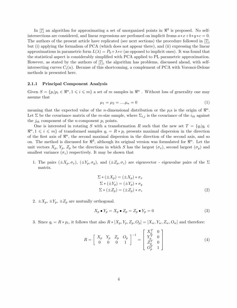
Given S = {pi|pi ∈ <n, 1 6 i 6 m} a set of m samples in <n . Without loss of generality one mayassume that

µ1 = µ2 = ....µn = 0 (1)

meaning that the expected value of the n-dimensional distribution or the pis is the origin of <n.Let Σ be the covariance matrix of the m-size sample, where Σi,j is the covariance of the ith againstthe jth component of the n-component pi points.

One is interested in rotating S with a transformation R such that the new set T = {qi|qi ∈<n, 1 6 i 6 m} of transformed samples qi = R ∗ pi presents maximal dispersion in the directionof the first axis of <n, the second maximal dispersion in the direction of the second axis, and soon. The method is discussed for <3, although its original version was formulated for <n. Let theunit vectors Xp, Yp, Zp be the directions in which S has the largest (σx), second largest (σy) andsmallest variance (σz) respectively. It may be shown that

1. The pairs (±Xp, σx), (±Yp, σy), and (±Zp, σz) are eigenvector - eigenvalue pairs of the Σmatrix.

Σ ∗ (±Xp) = (±Xp) ∗ σx

Σ ∗ (±Yp) = (±Yp) ∗ σy

Σ ∗ (±Zp) = (±Zp) ∗ σz (2)

2. ±Xp, ±Yp, ±Zp are mutually orthogonal.

Xp • Yp = Xp • Zp = Zp • Yp = 0 (3)

3. Since qi = R ∗ pi, it follows that also R ∗ [Xp, Yp, Zp, Op] = [Xw, Yw, Zw, Ow] and therefore:

R =[

Xp Yp Zp Op

0 0 0 1

]−1

=

XT

p 0Y T

p 0ZT

p 0OT

p 1

(4)

4

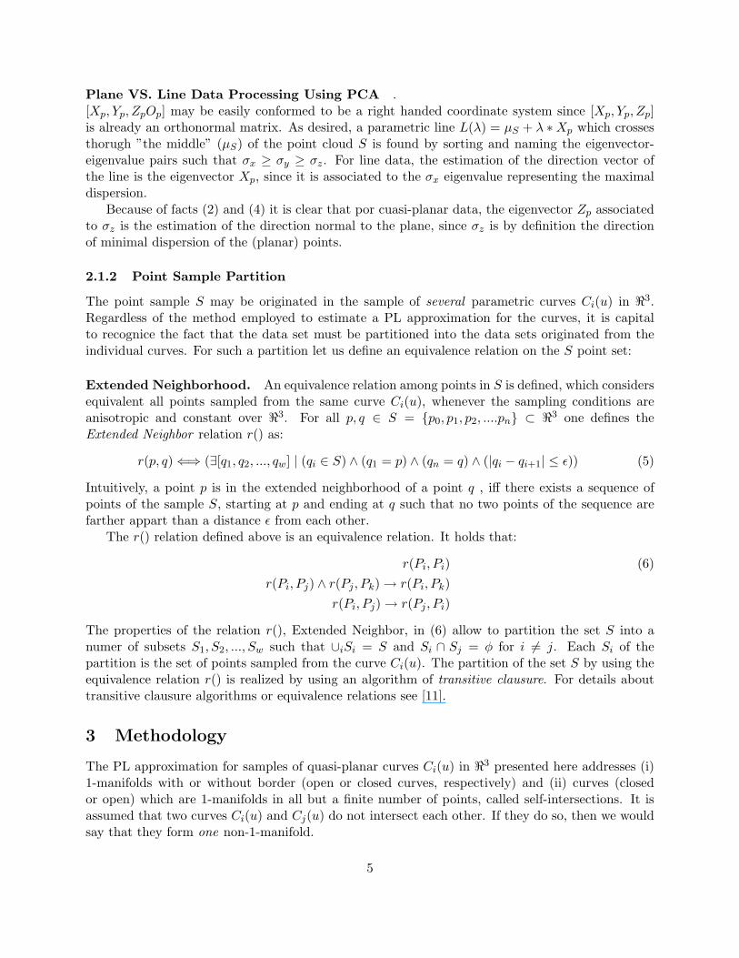
Plane VS. Line Data Processing Using PCA .[Xp, Yp, ZpOp] may be easily conformed to be a right handed coordinate system since [Xp, Yp, Zp]is already an orthonormal matrix. As desired, a parametric line L(λ) = µS + λ ∗Xp which crossesthorugh ”the middle” (µS) of the point cloud S is found by sorting and naming the eigenvector-eigenvalue pairs such that σx ≥ σy ≥ σz. For line data, the estimation of the direction vector ofthe line is the eigenvector Xp, since it is associated to the σx eigenvalue representing the maximaldispersion.

Because of facts (2) and (4) it is clear that por cuasi-planar data, the eigenvector Zp associatedto σz is the estimation of the direction normal to the plane, since σz is by definition the directionof minimal dispersion of the (planar) points.

2.1.2 Point Sample Partition

The point sample S may be originated in the sample of several parametric curves Ci(u) in <3.Regardless of the method employed to estimate a PL approximation for the curves, it is capitalto recognice the fact that the data set must be partitioned into the data sets originated from theindividual curves. For such a partition let us define an equivalence relation on the S point set:

Extended Neighborhood. An equivalence relation among points in S is defined, which considersequivalent all points sampled from the same curve Ci(u), whenever the sampling conditions areanisotropic and constant over <3. For all p, q ∈ S = {p0, p1, p2, ....pn} ⊂ <3 one defines theExtended Neighbor relation r() as:

r(p, q) ⇐⇒ (∃[q1, q2, ..., qw] | (qi ∈ S) ∧ (q1 = p) ∧ (qn = q) ∧ (|qi − qi+1| ≤ ε)) (5)

Intuitively, a point p is in the extended neighborhood of a point q , iff there exists a sequence ofpoints of the sample S, starting at p and ending at q such that no two points of the sequence arefarther appart than a distance ε from each other.

The r() relation defined above is an equivalence relation. It holds that:

r(Pi, Pi) (6)r(Pi, Pj) ∧ r(Pj , Pk) → r(Pi, Pk)

r(Pi, Pj) → r(Pj , Pi)

The properties of the relation r(), Extended Neighbor, in (6) allow to partition the set S into anumer of subsets S1, S2, ..., Sw such that ∪iSi = S and Si ∩ Sj = φ for i 6= j. Each Si of thepartition is the set of points sampled from the curve Ci(u). The partition of the set S by using theequivalence relation r() is realized by using an algorithm of transitive clausure. For details abouttransitive clausure algorithms or equivalence relations see [11].

3 Methodology

The PL approximation for samples of quasi-planar curves Ci(u) in <3 presented here addresses (i)1-manifolds with or without border (open or closed curves, respectively) and (ii) curves (closedor open) which are 1-manifolds in all but a finite number of points, called self-intersections. It isassumed that two curves Ci(u) and Cj(u) do not intersect each other. If they do so, then we wouldsay that they form one non-1-manifold.

5

Data Acquisition of curves Ci(u) in R3

S-2: raw point set

Ms: scalingmatrix

projection of point set S0 onto Π = [pv, n]

Delone Triangulation

PCA based best plane Π estimation

Point set scaling forhomogeneous bounding box

Delone TrianglesDT={ t1, t2,...,tn }

PCA estimation of local C’(u)

band = band ∪ (DT ∩∩∩∩ Bi ( µµµµi , f*Ri ))

S-1: norm. point set

S: planar point set

point set partition from individual Ci(u) samples

S0: sample for one Ci(u) curve

S setexhausted?

yes

no

Estimates ofRi: best ball radiusεi: local errorµµµµi: c(u) best ball centerXi : c’(u) tangent vector

band = { }

Bi+1

estimation

∪ j ∈ band ( tj )

Medial Axis Calculation

MA( P ) ≈≈≈≈ medial axis skeleton ≈ Ci(u)

Π = [pv, n] estimation

S: planar point set

S = S - (S ∩∩∩∩ Bi ( µµµµi , Ri ))

µµµµi+1: nextball center

(µµµµi , Xi )

band={ ti, tj,...,tw }⊂ DT

polygon P =∪ j ∈ band ( tj )

POINT SET PRE-PROCESSING

POLYGONAL COVERAGE OF S

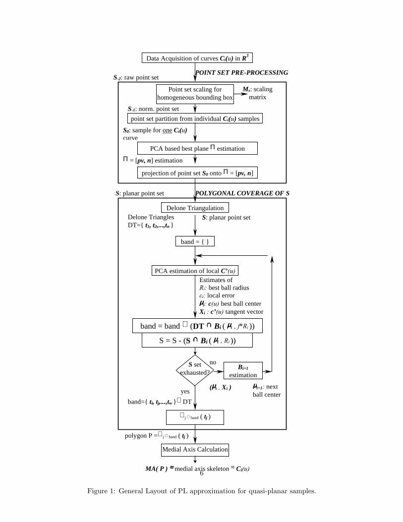
Figure 1: General Layout of PL approximation for quasi-planar samples.

6

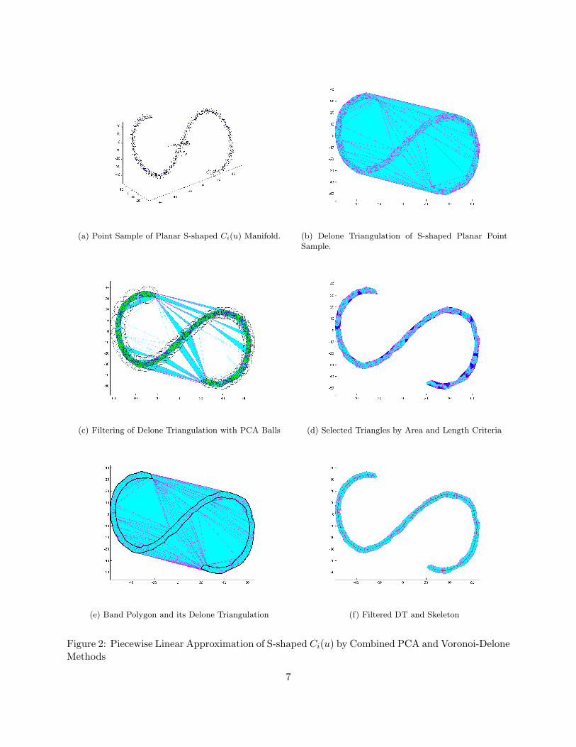
(a) Point Sample of Planar S-shaped Ci(u) Manifold. (b) Delone Triangulation of S-shaped Planar PointSample.

(c) Filtering of Delone Triangulation with PCA Balls (d) Selected Triangles by Area and Length Criteria

(e) Band Polygon and its Delone Triangulation (f) Filtered DT and Skeleton

Figure 2: Piecewise Linear Approximation of S-shaped Ci(u) by Combined PCA and Voronoi-DeloneMethods

7

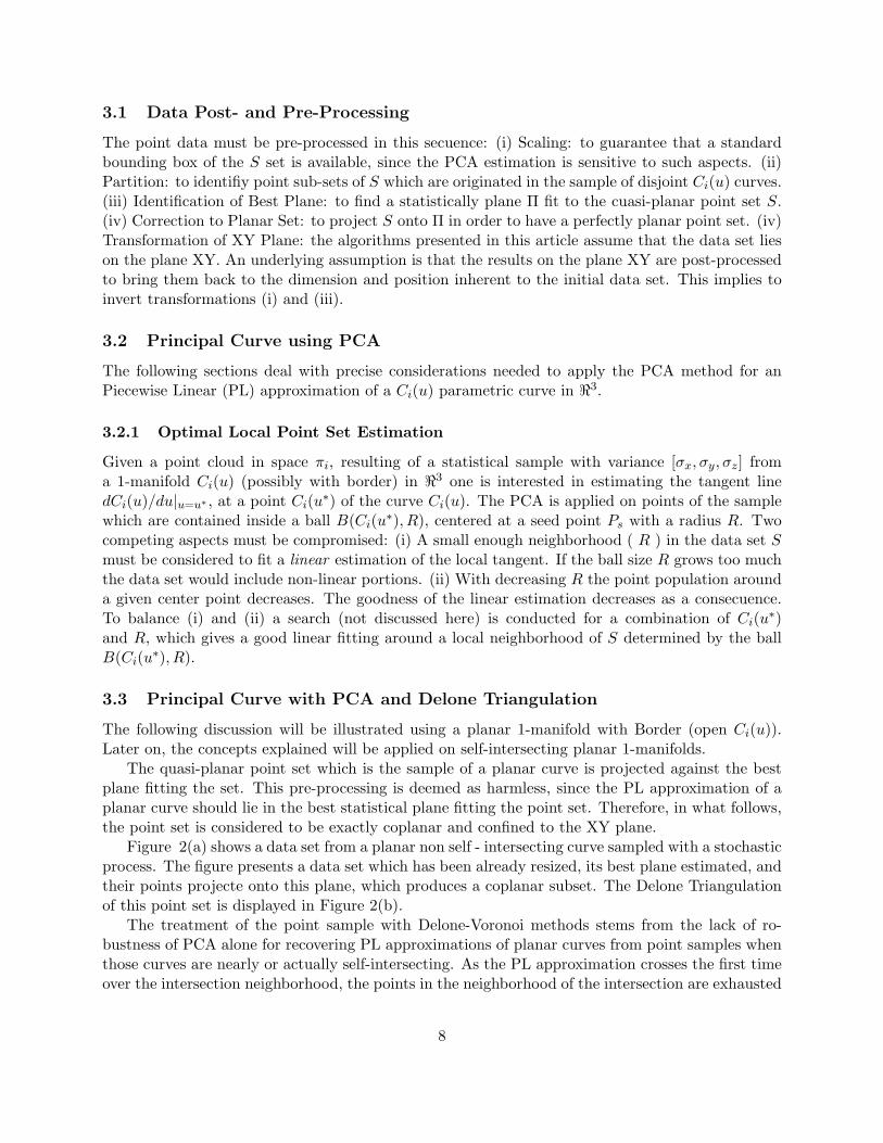
3.1 Data Post- and Pre-Processing

The point data must be pre-processed in this secuence: (i) Scaling: to guarantee that a standardbounding box of the S set is available, since the PCA estimation is sensitive to such aspects. (ii)Partition: to identifiy point sub-sets of S which are originated in the sample of disjoint Ci(u) curves.(iii) Identification of Best Plane: to find a statistically plane Π fit to the cuasi-planar point set S.(iv) Correction to Planar Set: to project S onto Π in order to have a perfectly planar point set. (iv)Transformation of XY Plane: the algorithms presented in this article assume that the data set lieson the plane XY. An underlying assumption is that the results on the plane XY are post-processedto bring them back to the dimension and position inherent to the initial data set. This implies toinvert transformations (i) and (iii).

3.2 Principal Curve using PCA

The following sections deal with precise considerations needed to apply the PCA method for anPiecewise Linear (PL) approximation of a Ci(u) parametric curve in <3.

3.2.1 Optimal Local Point Set Estimation

Given a point cloud in space πi, resulting of a statistical sample with variance [σx, σy, σz] froma 1-manifold Ci(u) (possibly with border) in <3 one is interested in estimating the tangent linedCi(u)/du|u=u∗ , at a point Ci(u∗) of the curve Ci(u). The PCA is applied on points of the samplewhich are contained inside a ball B(Ci(u∗), R), centered at a seed point Ps with a radius R. Twocompeting aspects must be compromised: (i) A small enough neighborhood ( R ) in the data set Smust be considered to fit a linear estimation of the local tangent. If the ball size R grows too muchthe data set would include non-linear portions. (ii) With decreasing R the point population arounda given center point decreases. The goodness of the linear estimation decreases as a consecuence.To balance (i) and (ii) a search (not discussed here) is conducted for a combination of Ci(u∗)and R, which gives a good linear fitting around a local neighborhood of S determined by the ballB(Ci(u∗), R).

3.3 Principal Curve with PCA and Delone Triangulation

The following discussion will be illustrated using a planar 1-manifold with Border (open Ci(u)).Later on, the concepts explained will be applied on self-intersecting planar 1-manifolds.

The quasi-planar point set which is the sample of a planar curve is projected against the bestplane fitting the set. This pre-processing is deemed as harmless, since the PL approximation of aplanar curve should lie in the best statistical plane fitting the point set. Therefore, in what follows,the point set is considered to be exactly coplanar and confined to the XY plane.

Figure 2(a) shows a data set from a planar non self - intersecting curve sampled with a stochasticprocess. The figure presents a data set which has been already resized, its best plane estimated, andtheir points projecte onto this plane, which produces a coplanar subset. The Delone Triangulationof this point set is displayed in Figure 2(b).

The treatment of the point sample with Delone-Voronoi methods stems from the lack of ro-bustness of PCA alone for recovering PL approximations of planar curves from point samples whenthose curves are nearly or actually self-intersecting. As the PL approximation crosses the first timeover the intersection neighborhood, the points in the neighborhood of the intersection are exhausted

8

for purposes of PCA estimation. As the PL curve revisits the intersection neighborhoods no pointsare available for identifying the trend of curve, and the algorithm tends to look for another point(i.e. curve) neighborhood were to work, withouth really having reproduced the intersection. Theresult is an incomplete curve stage, therefore missing the self-intersection detail.

Because of this reason, it was decided to determine a minimal polygon T covering S, the pointsample of Ci(u). T will resemble a tape (see Figure 2(e) ), and may have holes when covering closedor self-intersecting Ci(u). T is a subset of the Delone Triangulation DT (S) of the point set S (see[3] and [5]). In the present work, the triangle removal from DT (S) covering S is helped by the PCAestimations run on local neighborhoods of the point set S (see section 3.3.1). After T is obtained,an approximation of the medial axis of T is found. It is called called here a skeleton of T. Thisskeleton contains (in many cases it is) the PL approximation of the Ci(u) curve.

3.3.1 Filtering of Delone Triangles

The Delone Triangles will be filtered based on the following criteria: (a) Area, (b) Approximateenclosement in the PCA neighborhood (optimal ball), (c) Edge Length, (d) Vertex perpendiculardeparture from local tangent lines to Ci(u) and (e) Aspect Ratio. However, in order to applysuch methods ”reasonable values” of the area and edge length of Delone triangles belonging to Tneed to be estimated. For such purpose a PCA is run iteratively on neighborhoods of the dataset, thus determining the line ~L(λ) = ~Pv + λ ∗ v that best approaches the tangent to the Ci(u)curve in that neighborhood. Delone triangles contained within a scaled version of this ball, namelyB(Ci(u∗), fD ∗R) (with fD ≈ 1.3 an enlarging factor) might be considered as ”typical” of the onesforming the T , and therefore rendering ”typical area” A and ”typical edge length” l values. Thecriteria to classify a Delone triangle as belonging (or not belonging) to the tape are:

1. Enclosement: Accept a Delone triangle DTi if it is contained within the local PCA ball,that is, if DTi ⊆ B(Pv, Ro) where B(Pv, Ro) is the best local PCA ball (see Figure 2(c)).

2. Area and Edge Length: Reject a Delone triangle DTi if its Area or maximum Edge Lengthare too large. That is, if (Area(DTi) ≥ fA ∗ A) or if (Emax ≥ fl ∗ l) respectively, for constantsfA and fl. Figure 2(d) shows Delone Triangles surviving this criterium.

3.3.2 Polygon Synthesis based on Filtered Delone Triangulation

The approximation of the polygon T after application of criteria 1 and 2 is shown in Figure 2(d).As the Delone triangles DTk making up T are determined, their edges may have 1 or 2 triangleswhich are incident to it, with the following characteristics:

1. Edges ei,j in which two surviving Delone triangles DTi and DTj are incident are internal tothe tape-shaped 2D region.

2. Edges ei in which only one surviving Delone triangle DTi is incident constitute the boundary∂T of the 2D tape-shaped region T . They are either in the outermost loop, or in an internalloop.

The classification of internal vs external edges in a 2-manifold with boundary ([2], [9]) is charac-teristic of Boundary Representations. Additional information on Boundary Representation may befound in [8].

9

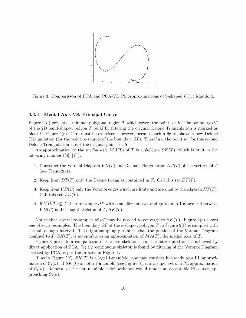
Figure 3: Comparisson of PCA and PCA-VD PL Approximations of S-shaped Ci(u) Manifold.

3.3.3 Medial Axis VS. Principal Curve

Figure 2(d) presents a minimal polygonal region T which covers the point set S. The boundary ∂Tof the 2D band-shaped polyon T build by filtering the original Delone Triangulation is marked asblack in Figure 2(e). Care must be exercised, however, because such a figure shows a new DeloneTriangulation (for the point re-sample of the boundary ∂T ). Therefore, the point set for this secondDelone Triangulation is not the original point set S.

An approximation to the medial axis MA(T ) of T is a skeleton SK(T ), which is built in thefollowing manner ([4], [1] ):

1. Construct the Voronoi Diagram V D(T ) and Delone Triangulation DT (T ) of the vertices of T(see Figure2(e)).

2. Keep from DT (T ) only the Delone triangles contained in T . Call this set DT (T ).

3. Keep from V D(T ) only the Voronoi edges which are finite and are dual to the edges in DT (T ).Call this set V D(T ).

4. If V D(T ) * T then re-sample ∂T with a smaller interval and go to step 1 above. Otherwise,V D(T ) is the sought skeleton of T , SK(T ).

Notice that several re-samples of ∂T may be needed to converge to SK(T ). Figure 2(e) showsone of such resamples. The boundary ∂T of the s-shaped polygon T in Figure 2(f) is sampled witha small enough interval. This tight sampling gurantees that the portion of the Voronoi Diagramconfined to T , SK(T ), is acceptable as an approximation of MA(T ), the medial axis of T .

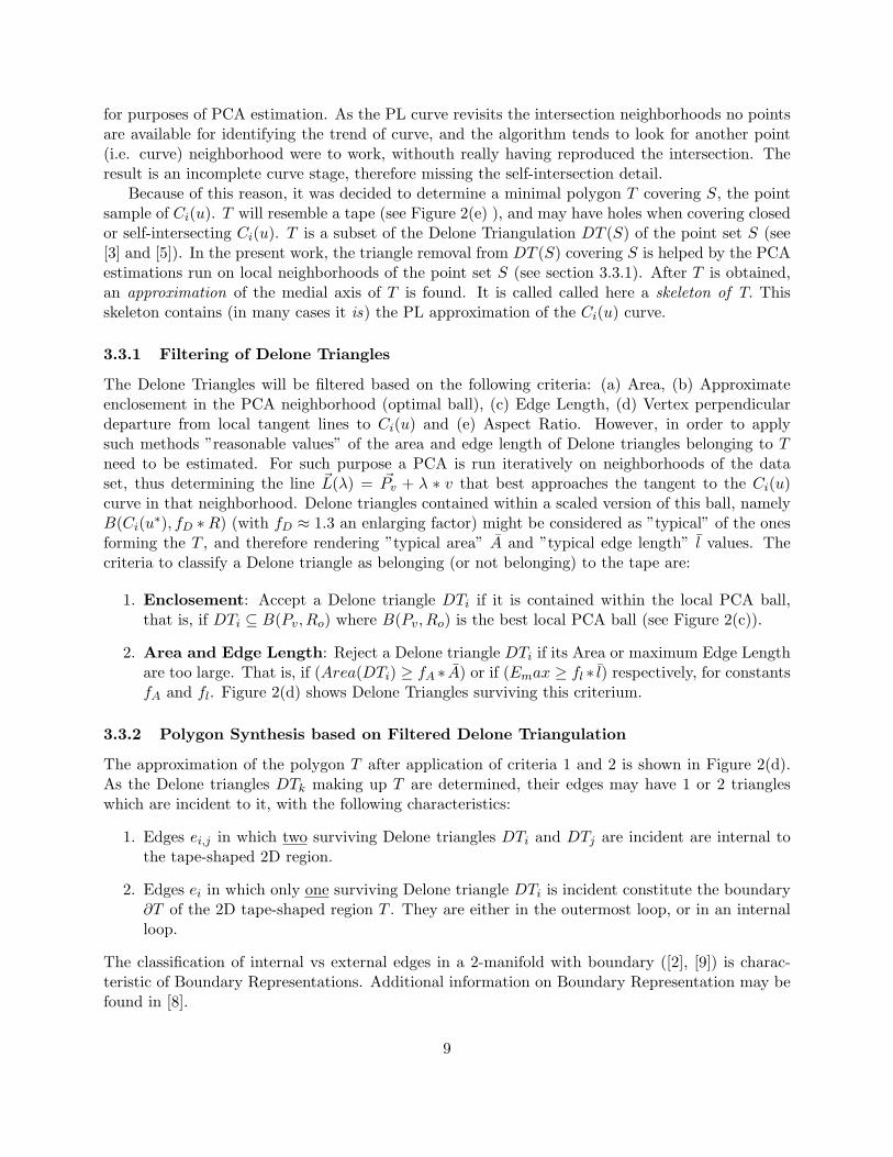
Figure 3 presents a comparisson of the two skeletons: (a) the interrupted one is achieved bydirect application of PCA. (b) the continuous skeleton is found by filtering of the Voronoi Diagramassisted by PCA as per the process in Figure 1.

If, as in Figure 2(f), SK(T ) is a legal 1-manifold, one may consider it already as a PL approxi-mation of Ci(u). If SK(T ) is not a 1-manifold (see Figure 5), it is a super-set of a PL approximationof Ci(u). Removal of the non-manifold neighborhoods would render an acceptable PL curve, ap-proaching Ci(u),

10

4 Results

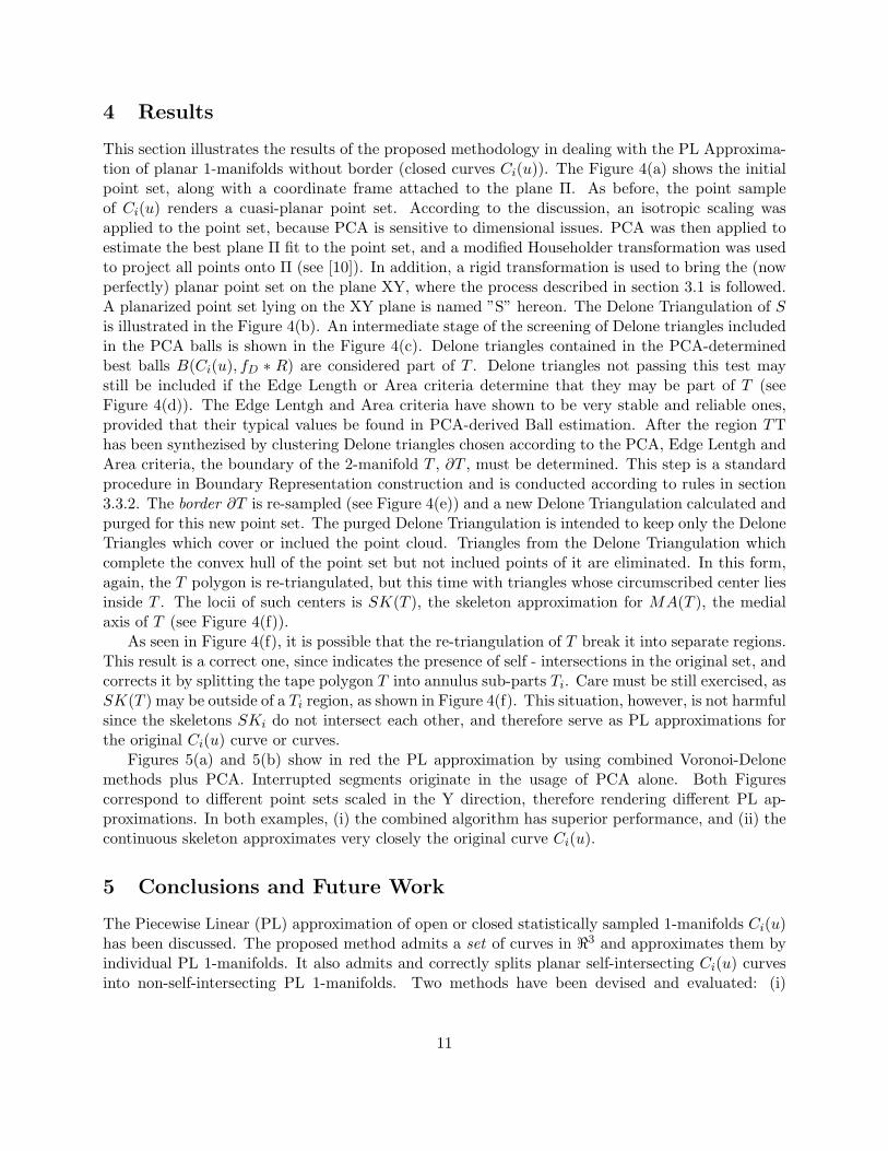
This section illustrates the results of the proposed methodology in dealing with the PL Approxima-tion of planar 1-manifolds without border (closed curves Ci(u)). The Figure 4(a) shows the initialpoint set, along with a coordinate frame attached to the plane Π. As before, the point sampleof Ci(u) renders a cuasi-planar point set. According to the discussion, an isotropic scaling wasapplied to the point set, because PCA is sensitive to dimensional issues. PCA was then applied toestimate the best plane Π fit to the point set, and a modified Householder transformation was usedto project all points onto Π (see [10]). In addition, a rigid transformation is used to bring the (nowperfectly) planar point set on the plane XY, where the process described in section 3.1 is followed.A planarized point set lying on the XY plane is named ”S” hereon. The Delone Triangulation of Sis illustrated in the Figure 4(b). An intermediate stage of the screening of Delone triangles includedin the PCA balls is shown in the Figure 4(c). Delone triangles contained in the PCA-determinedbest balls B(Ci(u), fD ∗ R) are considered part of T . Delone triangles not passing this test maystill be included if the Edge Length or Area criteria determine that they may be part of T (seeFigure 4(d)). The Edge Lentgh and Area criteria have shown to be very stable and reliable ones,provided that their typical values be found in PCA-derived Ball estimation. After the region TThas been synthezised by clustering Delone triangles chosen according to the PCA, Edge Lentgh andArea criteria, the boundary of the 2-manifold T , ∂T , must be determined. This step is a standardprocedure in Boundary Representation construction and is conducted according to rules in section3.3.2. The border ∂T is re-sampled (see Figure 4(e)) and a new Delone Triangulation calculated andpurged for this new point set. The purged Delone Triangulation is intended to keep only the DeloneTriangles which cover or inclued the point cloud. Triangles from the Delone Triangulation whichcomplete the convex hull of the point set but not inclued points of it are eliminated. In this form,again, the T polygon is re-triangulated, but this time with triangles whose circumscribed center liesinside T . The locii of such centers is SK(T ), the skeleton approximation for MA(T ), the medialaxis of T (see Figure 4(f)).

As seen in Figure 4(f), it is possible that the re-triangulation of T break it into separate regions.This result is a correct one, since indicates the presence of self - intersections in the original set, andcorrects it by splitting the tape polygon T into annulus sub-parts Ti. Care must be still exercised, asSK(T ) may be outside of a Ti region, as shown in Figure 4(f). This situation, however, is not harmfulsince the skeletons SKi do not intersect each other, and therefore serve as PL approximations forthe original Ci(u) curve or curves.

Figures 5(a) and 5(b) show in red the PL approximation by using combined Voronoi-Delonemethods plus PCA. Interrupted segments originate in the usage of PCA alone. Both Figurescorrespond to different point sets scaled in the Y direction, therefore rendering different PL ap-proximations. In both examples, (i) the combined algorithm has superior performance, and (ii) thecontinuous skeleton approximates very closely the original curve Ci(u).

5 Conclusions and Future Work

The Piecewise Linear (PL) approximation of open or closed statistically sampled 1-manifolds Ci(u)has been discussed. The proposed method admits a set of curves in <3 and approximates them byindividual PL 1-manifolds. It also admits and correctly splits planar self-intersecting Ci(u) curvesinto non-self-intersecting PL 1-manifolds. Two methods have been devised and evaluated: (i)

11

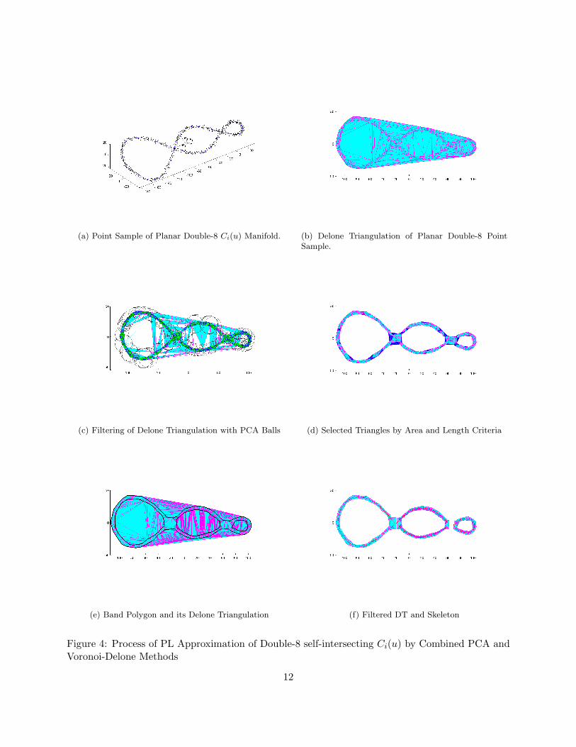
(a) Point Sample of Planar Double-8 Ci(u) Manifold. (b) Delone Triangulation of Planar Double-8 PointSample.

(c) Filtering of Delone Triangulation with PCA Balls (d) Selected Triangles by Area and Length Criteria

(e) Band Polygon and its Delone Triangulation (f) Filtered DT and Skeleton

Figure 4: Process of PL Approximation of Double-8 self-intersecting Ci(u) by Combined PCA andVoronoi-Delone Methods

12

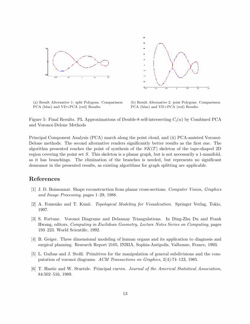
(a) Result Alternative 1: split Polygons. ComparissonPCA (blue) and VD+PCA (red) Results

(b) Result Alternative 2: joint Polygons. ComparissonPCA (blue) and VD+PCA (red) Results

Figure 5: Final Results. PL Approximations of Double-8 self-intersecting Ci(u) by Combined PCAand Voronoi-Delone Methods

Principal Component Analysis (PCA) march along the point cloud, and (ii) PCA-assisted Voronoi-Delone methods. The second alternative renders significantly better results as the first one. Thealgorithm presented reaches the point of synthesis of the SK(T ) skeleton of the tape-shaped 2Dregion covering the point set S. This skeleton is a planar graph, but is not necessarily a 1-manifold,as it has branchings. The elimination of the branches is needed, but represents no significantdemeanor in the presented results, as existing algorithms for graph splitting are applicable.

References

[1] J. D. Boissonnat. Shape reconstruction from planar cross-sections. Computer Vision, Graphicsand Image Processing, pages 1–29, 1988.

[2] A. Fomenko and T. Kunii. Topological Modeling for Visualization. Springer Verlag, Tokio,1997.

[3] S. Fortune. Voronoi Diagrams and Delaunay Triangulations. In Ding-Zhu Du and FrankHwang, editors, Computing in Euclidean Geometry, Lecture Notes Series on Computing, pages193–223. World Scientific, 1992.

[4] B. Geiger. Three dimensional modeling of human organs and its application to diagnosis andsurgical planning. Research Report 2105, INRIA, Sophia-Antipolis, Valbonne, France, 1993.

[5] L. Guibas and J. Stolfi. Primitives for the manipulation of general subdivisions and the com-putation of voronoi diagrams. ACM Transactions on Graphics, 2(4):74–123, 1985.

[6] T. Hastie and W. Stuetzle. Principal curves. Journal of the Americal Statistical Association,84:502–516, 1989.

13

[7] I. Lee. Curve reconsruction from unorganized points. Computer Aided Geometric Design,17:161–177, 2000.

[8] M. Mantyla. An Introduction to Solid Modeling. Computer Science Press, Maryland, USA,1988.

[9] M. Morse. The calculus of variations in the large. American Mathematical Society, New York,1934.

[10] O. Ruiz. Understanding CAD / CAM / CG. American Society of Mechanical Engineers ASME.Continuing Education Institute. Global Training, 2002. ASME Code GT-006.

[11] P. Suppes. Axiomatic Set Theory. Dover Publishing, New York, 1972.

14