Approximating implicit curves on plane and surface triangulations with affine arithmetic

Filipe de Carvalho Nascimentoa, Afonso Paivaa, Luiz Henrique de Figueiredob, Jorge Stolfic

aInstituto de Ciencias Matematicas e de Computacao, Universidade de Sao Paulo, Sao Carlos, BrazilbInstituto Nacional de Matematica Pura e Aplicada, Rio de Janeiro, Brazil

cInstituto de Computacao, Universidade Estadual de Campinas, Campinas, Brazil

Abstract

We present a spatially and geometrically adaptive method for computing a robust polygonal approximation of an implicit curvedefined on a planar region or on a triangulated surface. Our method uses affine arithmetic to identify regions where the curve liesinside a thin strip. Unlike other interval methods, even those based on affine arithmetic, our method works on both rectangular andtriangular decompositions and can use any refinement scheme that the decomposition offers.

Keywords: implicit curves, polygonal approximation, interval methods.

1. Introduction

The numerical solution of systems of non-linear equationsin several variables is a key tool in geometric modeling andcomputer-aided geometric design [1]. In many applications,such as surface intersection and offset computation, the solutionis not a set of isolated points but rather a curve or a surface. Thesimplest case is the solution of an equation f (x,y) = 0, whichgives an implicit curve on the plane.

Computing a polygonal approximation of an implicit curveis a challenging problem because it is difficult to find points onthe curve and also because the curve may have several connectedcomponents. Therefore, robust approximation algorithms mustexplore the whole region of interest to avoid missing any com-ponents of the curve. One approach for achieving robustnessis to use interval methods [2, 3], which are able to probe thebehavior of a function over whole regions instead of relyingon point sampling. Interval methods lead naturally to spatiallyadaptive solutions that concentrate efforts near the curve.

Several interval methods have been proposed for robustlyapproximating an implicit curve on the plane (see §2). Thesemethods explore a rectangular region of interest by decomposingit recursively and adaptively with a quadtree and using intervalestimates for the values of f (and sometimes of its gradient) ona cell as a subdivision criterion.

Affine arithmetic (AA) [4] is a generalization of classicalinterval arithmetic that explicitly represents first-order partialcorrelations, which can improve the convergence of intervalestimates. Some methods have used AA for approximatingimplicit curves, successfully exhibiting improved convergence,but none has exploited the additional geometric informationprovided by AA and none has worked on triangulations. Indeed,while all interval methods can compute interval estimates onrectangular cells, classical interval arithmetic cannot handletriangles naturally, except by enclosing them in axis-alignedrectangles. Thus, existing interval methods are restricted torectangular regions. Moreover, to handle implicit curves on

triangulated surfaces, these methods would have to use a 3d axis-aligned box containing each triangle, which is wasteful.

In this paper, we describe an interval method for adaptivelyapproximating an implicit curve on a refinable triangular decom-position of the region of interest. Our method uses the geometricinformation provided by AA as a flatness criterion to stop therecursion and is thus both spatially and geometrically adaptivein the sense of Lopes et al. [5]. Our method can handle implicitcurves given by algebraic or transcendental formulas, works ontriangulated plane regions and surfaces of arbitrary genus, andcan use any mesh refinement scheme. Fig. 1 shows an exampleof our method in action on a triangulated surface. Note how themesh is refined near the implicit curve.

After briefly reviewing some of the related work in §2 andthe main concepts of AA in §3, we explain in detail in §4 howto use AA to extract geometric estimates in the form of stripsfor the location of the curve in a triangle. This is the basis ofan interval method that can be used on triangulations, both onthe plane and on surfaces, which we present in §5. We discusssome examples of our method in action in §6 and we report ourconclusions and suggest directions for future work in §7.

A previous version of this paper [6] focused on plane curvesonly. Here, we focus on curves on surfaces. We also discussplane curves for motivation, simplicity of exposition, and com-pleteness. In addition to the material on surfaces presentedin §4.4 and §6, we include a performance comparison of thestrategies for handling triangles with AA in §4.3 and an ex-panded and detailed explanation of how our method works in §5.

2. Related work

Dobkin et al. [7] described in detail a continuation methodfor polygonal approximation of implicit curves in regular trian-gular grids generated by reflections. Since the grid is regular,their approximation is not adaptive. The selection of the gridresolution is left to the user. Persiano et al. [8] presented a gen-eral scheme for adaptive triangulation refinement which they

Preprint submitted to Computers & Graphics (second revised version) February 21, 2014

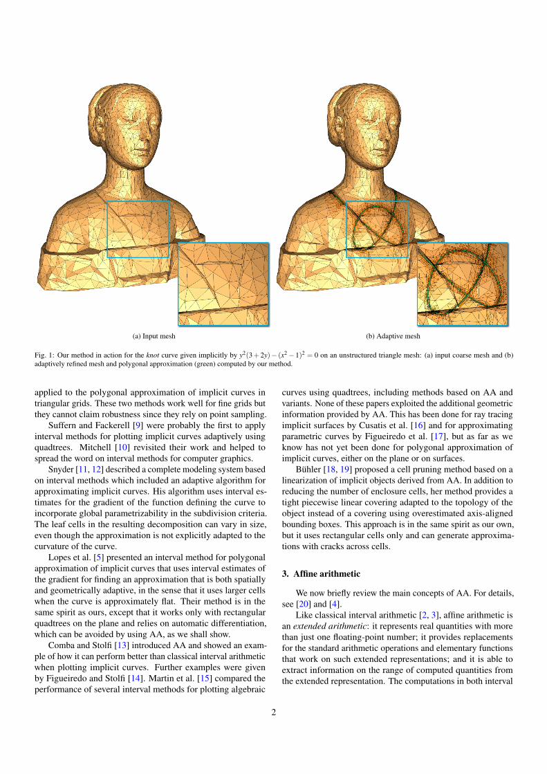
(a) Input mesh (b) Adaptive mesh

Fig. 1: Our method in action for the knot curve given implicitly by y2(3+ 2y)− (x2− 1)2 = 0 on an unstructured triangle mesh: (a) input coarse mesh and (b)adaptively refined mesh and polygonal approximation (green) computed by our method.

applied to the polygonal approximation of implicit curves intriangular grids. These two methods work well for fine grids butthey cannot claim robustness since they rely on point sampling.

Suffern and Fackerell [9] were probably the first to applyinterval methods for plotting implicit curves adaptively usingquadtrees. Mitchell [10] revisited their work and helped tospread the word on interval methods for computer graphics.

Snyder [11, 12] described a complete modeling system basedon interval methods which included an adaptive algorithm forapproximating implicit curves. His algorithm uses interval es-timates for the gradient of the function defining the curve toincorporate global parametrizability in the subdivision criteria.The leaf cells in the resulting decomposition can vary in size,even though the approximation is not explicitly adapted to thecurvature of the curve.

Lopes et al. [5] presented an interval method for polygonalapproximation of implicit curves that uses interval estimates ofthe gradient for finding an approximation that is both spatiallyand geometrically adaptive, in the sense that it uses larger cellswhen the curve is approximately flat. Their method is in thesame spirit as ours, except that it works only with rectangularquadtrees on the plane and relies on automatic differentiation,which can be avoided by using AA, as we shall show.

Comba and Stolfi [13] introduced AA and showed an exam-ple of how it can perform better than classical interval arithmeticwhen plotting implicit curves. Further examples were givenby Figueiredo and Stolfi [14]. Martin et al. [15] compared theperformance of several interval methods for plotting algebraic

curves using quadtrees, including methods based on AA andvariants. None of these papers exploited the additional geometricinformation provided by AA. This has been done for ray tracingimplicit surfaces by Cusatis et al. [16] and for approximatingparametric curves by Figueiredo et al. [17], but as far as weknow has not yet been done for polygonal approximation ofimplicit curves, either on the plane or on surfaces.

Buhler [18, 19] proposed a cell pruning method based on alinearization of implicit objects derived from AA. In addition toreducing the number of enclosure cells, her method provides atight piecewise linear covering adapted to the topology of theobject instead of a covering using overestimated axis-alignedbounding boxes. This approach is in the same spirit as our own,but it uses rectangular cells only and can generate approxima-tions with cracks across cells.

3. Affine arithmetic

We now briefly review the main concepts of AA. For details,see [20] and [4].

Like classical interval arithmetic [2, 3], affine arithmetic isan extended arithmetic: it represents real quantities with morethan just one floating-point number; it provides replacementsfor the standard arithmetic operations and elementary functionsthat work on such extended representations; and it is able toextract information on the range of computed quantities fromthe extended representation. The computations in both interval

2

and affine arithmetic take into account all rounding errors infloating-point arithmetic and so provide reliable results.

Interval arithmetic uses two floating-point numbers to repre-sents intervals containing quantities. Affine arithmetic representsa quantity q with an affine form:

q = q0 +q1ε1 +q2ε2 + · · ·+qnεn

where qi are real numbers and εi are noise symbols which varyin the interval [−1,1] and represent independent sources of un-certainty. From this representation, one deduces an intervalestimate for the value of q:

q ∈ [q] := [q0−δ ,q0 +δ ]

where δ = |q1|+ · · ·+ |qn|. Thus, AA generalizes interval arith-metic. More importantly, by design affine forms can share noisesymbols and thus may be not completely independent. The ex-plicit representation of first-order partial correlations and thequadratic convergence of estimates are the main features of AAthat are absent in classical interval arithmetic. Despite the in-creased computational cost in AA, these features yield moreefficient methods in several cases, especially when the geometryof AA approximations is exploited [16, 17], as in this paper.

There are simple formulas for operating with affine forms.The formulas for affine operations (addition, subtraction, scalarmultiplication, and scalar translation) are immediate, becauseaffine forms represent these operations exactly (except for round-ing errors in floating-point arithmetic). The formulas for non-affine operations (multiplication, integer powers, square root,and other elementary functions) rely on a good affine approxima-tion with an explicit error term, as explained in detail elsewhere[20, 4]. By combining the formulas for these basic operations,one can evaluate any complicated algebraic or transcendentalformula on affine forms. As in other extended arithmetics, this isespecially convenient to implement automatically using operatoroverloading, which is readily available in several programminglanguages. We use libaffa, a C++ library for AA [21].

4. Bounding implicit curves with strips

Affine forms have a rich geometry, which our method triesto exploit. We now describe how to use AA to compute a stripof parallel lines that contains the piece of the plane curve givenimplicitly by f (x,y) = 0 in axis-aligned rectangles, arbitrary par-allelograms, and triangles. We then explain how to extend thiscomputation to handle a curve given implicitly by f (x,y,z) = 0on a triangulated surface. This is the basis of our adaptive ap-proximation method, which we present in §5.

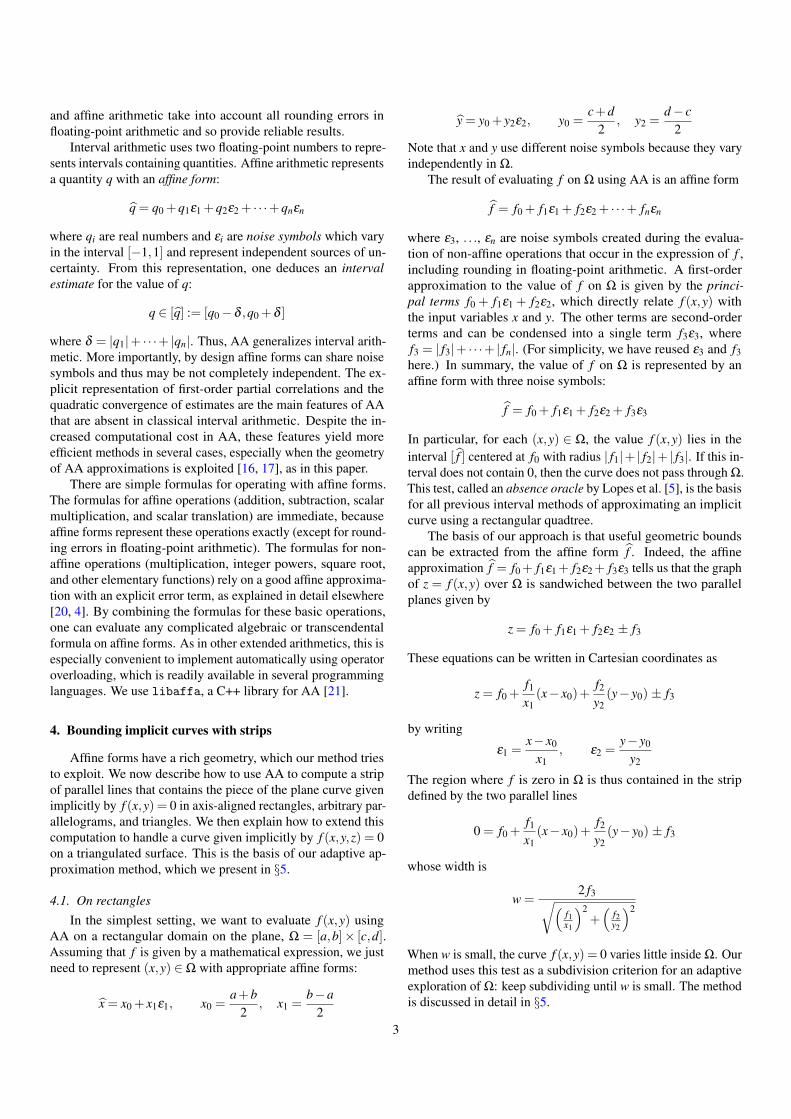
4.1. On rectanglesIn the simplest setting, we want to evaluate f (x,y) using

AA on a rectangular domain on the plane, Ω = [a,b]× [c,d].Assuming that f is given by a mathematical expression, we justneed to represent (x,y) ∈Ω with appropriate affine forms:

x = x0 + x1ε1, x0 =a+b

2, x1 =

b−a2

y = y0 + y2ε2, y0 =c+d

2, y2 =

d− c2

Note that x and y use different noise symbols because they varyindependently in Ω.

The result of evaluating f on Ω using AA is an affine form

f = f0 + f1ε1 + f2ε2 + · · ·+ fnεn

where ε3, . . ., εn are noise symbols created during the evalua-tion of non-affine operations that occur in the expression of f ,including rounding in floating-point arithmetic. A first-orderapproximation to the value of f on Ω is given by the princi-pal terms f0 + f1ε1 + f2ε2, which directly relate f (x,y) withthe input variables x and y. The other terms are second-orderterms and can be condensed into a single term f3ε3, wheref3 = | f3|+ · · ·+ | fn|. (For simplicity, we have reused ε3 and f3here.) In summary, the value of f on Ω is represented by anaffine form with three noise symbols:

f = f0 + f1ε1 + f2ε2 + f3ε3

In particular, for each (x,y) ∈ Ω, the value f (x,y) lies in theinterval [ f ] centered at f0 with radius | f1|+ | f2|+ | f3|. If this in-terval does not contain 0, then the curve does not pass through Ω.This test, called an absence oracle by Lopes et al. [5], is the basisfor all previous interval methods of approximating an implicitcurve using a rectangular quadtree.

The basis of our approach is that useful geometric boundscan be extracted from the affine form f . Indeed, the affineapproximation f = f0+ f1ε1+ f2ε2+ f3ε3 tells us that the graphof z = f (x,y) over Ω is sandwiched between the two parallelplanes given by

z = f0 + f1ε1 + f2ε2 ± f3

These equations can be written in Cartesian coordinates as

z = f0 +f1

x1(x− x0)+

f2

y2(y− y0) ± f3

by writing

ε1 =x− x0

x1, ε2 =

y− y0

y2

The region where f is zero in Ω is thus contained in the stripdefined by the two parallel lines

0 = f0 +f1

x1(x− x0)+

f2

y2(y− y0) ± f3

whose width is

w =2 f3√(

f1x1

)2+(

f2y2

)2

When w is small, the curve f (x,y) = 0 varies little inside Ω. Ourmethod uses this test as a subdivision criterion for an adaptiveexploration of Ω: keep subdividing until w is small. The methodis discussed in detail in §5.

3

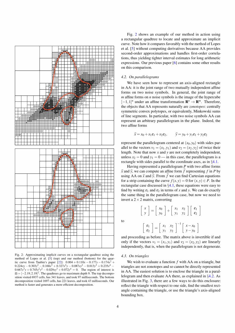
Fig. 2: Approximating implicit curves on a rectangular quadtree using themethod of Lopes et al. [5] (top) and our method (bottom) for the quar-tic curve from Taubin’s paper [22]: 0.004 + 0.110x− 0.177y− 0.174x2 +0.224xy − 0.303y2 − 0.168x3 + 0.327x2y − 0.087xy2 − 0.013y3 + 0.235x4 −0.667x3y + 0.745x2y2 − 0.029xy3 + 0.072y4 = 0. The region of interest isΩ = [−2.19,2.19]2. The quadtrees go to maximum depth 9. The top decompo-sition visited 6937 cells, has 341 leaves, and took 97 milliseconds. The bottomdecomposition visited 1697 cells, has 221 leaves, and took 43 milliseconds. Ourmethod is faster and generates a more efficient decomposition.

Fig. 2 shows an example of our method in action usinga rectangular quadtree to locate and approximate an implicitcurve. Note how it compares favorably with the method of Lopeset al. [5] without computing derivatives because AA providessecond-order approximations and handles first-order correla-tions, thus yielding tighter interval estimates for long arithmeticexpressions. Our previous paper [6] contains some other resultson this comparison.

4.2. On parallelograms

We have seen how to represent an axis-aligned rectanglein AA: it is the joint range of two mutually independent affineforms on two noise symbols. In general, the joint range ofm affine forms on n noise symbols is the image of the hypercube[−1,1]n under an affine transformation Rn → Rm. Therefore,the objects that AA represents naturally are zonotopes: centrallysymmetric convex polytopes, or equivalently, Minkowski sumsof line segments. In particular, with two noise symbols AA canrepresent an arbitrary parallelogram in the plane. Indeed, thetwo affine forms

x = x0 + x1ε1 + x2ε2, y = y0 + y1ε1 + y2ε2

represent the parallelogram centered at (x0,y0) with sides par-allel to the vectors v1 = (x1,y1) and v2 = (x2,y2) of twice theirlength. Note that now x and y are not completely independent,unless x2 = 0 and y1 = 0 — in this case, the parallelogram is arectangle with sides parallel to the coordinate axes, as in §4.1.

Having represented a parallelogram P with two affine formsx and y, we can compute an affine form f representing f in P byusing AA on x and y. From f we can find Cartesian equationsfor a strip containing the curve f (x,y) = 0 for (x,y) ∈ P. In therectangular case discussed in §4.1, these equations were easy tofind by writing ε1 and ε2 in terms of x and y. We can do exactlythe same thing in the parallelogram case, but now we need toinvert a 2×2 matrix, converting[

xy

]=

[x0y0

]+

[x1 x2y1 y2

][ε1ε2

]to [

ε1ε2

]=

[x1 x2y1 y2

]−1 [ x− x0y− y0

]and proceeding as before. The matrix above is invertible if andonly if the vectors v1 = (x1,y1) and v2 = (x2,y2) are linearlyindependently, that is, when the parallelogram is not degenerate.

4.3. On triangles

We wish to evaluate a function f with AA on a triangle, buttriangles are not zonotopes and so cannot be directly representedin AA. The easiest solution is to enclose the triangle in a paral-lelogram and then evaluate AA there, as explained in §4.2. Asillustrated in Fig. 3, there are a few ways to do this enclosure:reflect the triangle with respect to one side, find the smallest rect-angle containing the triangle, or use the triangle’s axis-alignedbounding box.

4

(a) (b) (c) (d) (e)

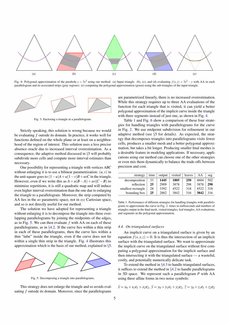
Fig. 4: Polygonal approximation of the parabola y = 3x2 using our method. (a) Input triangle. (b), (c), and (d) evaluating f (x,y) = 3x2− y with AA in eachparallelogram and its associated strips (gray regions). (e) computing the polygonal approximation (green) using the sub-triangles of the input triangle.

Fig. 3: Enclosing a triangle in a parallelogram.

Strictly speaking, this solution is wrong because we wouldbe evaluating f outside its domain. In practice, it works well forfunctions defined on the whole plane or at least on a neighbor-hood of the region of interest. This solution uses a less preciseabsence oracle due to increased interval overestimation. As aconsequence, the adaptive method discussed in §5 will probablysubdivide more cells and compute more interval estimates thannecessary.

One possibility for representing a triangle with vertices ABCwithout enlarging it is to use a bilinear parametrization: (u,v) inthe unit square goes to (1−u)A+u(1−v)B+uvC in the triangle.However, even if we write this as A+u(B−A)+uv(C−B) tominimize repetitions, it is still a quadratic map and will induceeven higher interval overestimation than the one due to enlargingthe triangle to a parallelogram. Moreover, the strip computed byAA lies in the uv parametric space, not in xyz Cartesian space,and so is not directly useful for our method.

The solution we have adopted for representing a trianglewithout enlarging it is to decompose the triangle into three over-lapping parallelograms by joining the midpoints of the edges,as in Fig. 5. We can then evaluate f with AA on each of theseparallelograms, as in §4.2. If the curve lies within a thin stripin each of these parallelograms, then the curve lies within athin “tube” inside the triangle, even if the curve does not liewithin a single thin strip in the triangle. Fig. 4 illustrates thisapproximation which is the basis of our method, explained in §5.

Fig. 5: Decomposing a triangle into parallelograms.

This strategy does not enlarge the triangle and so avoids eval-uating f outside its domain. Moreover, since the parallelograms

are parametrized linearly, there is no increased overestimation.While this strategy requires up to three AA evaluations of thefunction for each triangle that is visited, it can yield a betterpolygonal approximation of the implicit curve inside the trianglewith three segments instead of just one, as shown in Fig. 4.

Table 1 and Fig. 6 show a comparison of these four strate-gies for handling triangles with parallelograms for the curvein Fig. 2. We use midpoint subdivision for refinement in ouradaptive method (see §5 for details). As expected, the strat-egy that decomposes triangles into parallelograms visits fewercells, produces a smaller mesh and a better polygonal approxi-mation, but takes a bit longer. Producing smaller final meshes isa desirable feature in modeling applications. If necessary, appli-cations using our method can choose one of the other strategiesor even mix them dynamically to balance the trade-offs betweenprecision and cost.

strategy time output visited leaves AA segdecomposition 33 1445 1805 250 4604 502

reflection 25 2909 3878 298 3878 298smallest rectangle 28 3392 4522 318 4522 318

bounding box 25 2882 3842 316 3842 316

Table 1: Performance of different strategies for handling triangles with parallelo-grams to approximate the curve in Fig. 2: times in milliseconds and numbers oftriangles output in the final mesh, visited triangles, leaf triangles, AA evaluations,and segments in the polygonal approximation.

4.4. On triangulated surfaces

An implicit curve on a triangulated surface is given by anequation f (x,y,z) = 0. It is thus the intersection of an implicitsurface with the triangulated surface. We want to approximatethe implicit curve on the triangulated surface without first com-puting a polygonal approximation for the implicit surface andthen intersecting it with the triangulated surface — a wasteful,costly, and potentially numerically delicate task.

To extend the method in §4.3 to handle triangulated surfaces,it suffices to extend the method in §4.2 to handle parallelogramsin 3D space. We represent such a parallelogram P with AAusing three affine forms in two noise symbols:

x = x0 +x1ε1 +x2ε2, y = y0 +y1ε1 +y2ε2, z = z0 + z1ε1 + z2ε2

5

(a) decomposition (b) reflection (c) smallest rectangle (d) bounding box

Fig. 6: Effect of different strategies for handling triangles with parallelograms to approximate the curve of Fig. 2.

As before, evaluating f (x,y,z) using AA on P yields that theimplicit curve f (x,y,z) = 0 in P lies sandwiched between thetwo parallel planes given by

0 = f0 + f1ε1 + f2ε2 ± f3

Again, we translate these equations into Cartesian coordinatesby writing ε1 and ε2 in terms of x, y, z. More precisely, from x

yz

=

x0y0z0

+ x1 x2

y1 y2z1 z2

[ ε1ε2

]we get [

ε1ε2

]=

x1 x2y1 y2z1 z2

+ x− x0y− y0z− z0

where B+ = (B>B)−1B> is the pseudoinverse of a matrix B.This expression for the pseudoinverse is valid exactly when thematrix has full rank, that is, when its two columns are linearlyindependent. In geometric terms, this happens exactly when theparallelogram P is not degenerate.

5. Our adaptive method

Once we know how to decide whether an implicit curve canbe well approximated by a strip or a series of strips inside a cell(be it a rectangle, a parallelogram, or a triangle), we can usethis test as a criterion for adaptive subdivision: if the curve iswell approximated inside the cell, then we stop the subdivision;otherwise, we decompose the current cell into a number ofsubcells and recursively explore each subcell.

Our method is summarized in Fig. 7, in two versions: onefor parallelograms, including rectangles, and one for triangles.The method starts with procedure Adaptive which explores eachcell in an initial mesh decomposition of the region of interest orsurface. For rectangular quadtrees in the plane, the initial meshtypically contains a single cell. For triangular decompositions ofrectangular regions in the plane, the initial mesh typically con-tains two cells dividing the rectangle diagonally. Nevertheless,the method works for arbitrary triangulated regions and surfaces.

The core of the method is the Explore procedure whichrecursively tests whether the curve crosses the cell, subdividing

procedure Adaptive()for all cells C in the base mesh do

Explore(C)end

procedure Explore(C) (parallelograms)f ← f (C) with AAif 0 ∈ [ f ] then

w← width of f in Cif w≤ ε then

Approximate(C)else

divide C into subcells Cifor each i, Explore(Ci)

end

procedure Explore(C) (triangles)P1,P2,P3← parallelograms of Cfi← f (Pi) with AAif 0 ∈ [ fi] for some i then

wi← width of f in Piif wi ≤ ε for all i then

Approximate(C)else

divide C into subcells Cifor each i, Explore(Ci)

end

Fig. 7: Our adaptive method summarized.

the cell as needed. The recursion stops when the curve doesnot cross the cell (as proved by the interval estimate [ f ] notcontaining zero), when the curve lies within a thin tube insidethe cell (of width less than a user-supplied tolerance ε), or whena maximum recursion depth has been reached, for safety.

In the case of triangles, Explore is rearranged to test eachparallelogram in sequence, avoiding further tests as soon as thecurve is not thin inside a parallelogram. The triangle is thenimmediately subdivided and explored recursively. This changecan avoid many unnecessary AA evaluations.

When the curve lies in a thin tube, we perform the Approxi-mate procedure, in which we compute a polygonal approxima-

6

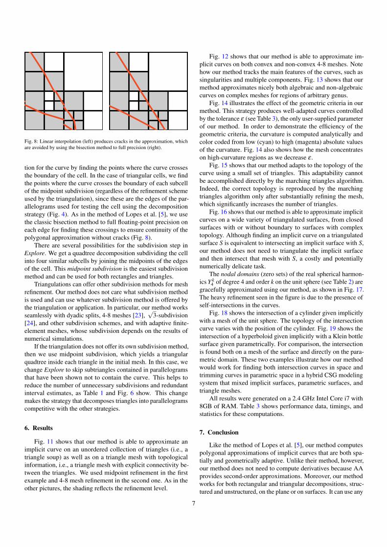
Fig. 8: Linear interpolation (left) produces cracks in the approximation, whichare avoided by using the bisection method to full precision (right).

tion for the curve by finding the points where the curve crossesthe boundary of the cell. In the case of triangular cells, we findthe points where the curve crosses the boundary of each subcellof the midpoint subdivision (regardless of the refinement schemeused by the triangulation), since these are the edges of the par-allelograms used for testing the cell using the decompositionstrategy (Fig. 4). As in the method of Lopes et al. [5], we usethe classic bisection method to full floating-point precision oneach edge for finding these crossings to ensure continuity of thepolygonal approximation without cracks (Fig. 8).

There are several possibilities for the subdivision step inExplore. We get a quadtree decomposition subdividing the cellinto four similar subcells by joining the midpoints of the edgesof the cell. This midpoint subdivision is the easiest subdivisionmethod and can be used for both rectangles and triangles.

Triangulations can offer other subdivision methods for meshrefinement. Our method does not care what subdivision methodis used and can use whatever subdivision method is offered bythe triangulation or application. In particular, our method worksseamlessly with dyadic splits, 4-8 meshes [23],

√3-subdivision

[24], and other subdivision schemes, and with adaptive finite-element meshes, whose subdivision depends on the results ofnumerical simulations.

If the triangulation does not offer its own subdivision method,then we use midpoint subdivision, which yields a triangularquadtree inside each triangle in the initial mesh. In this case, wechange Explore to skip subtriangles contained in parallelogramsthat have been shown not to contain the curve. This helps toreduce the number of unnecessary subdivisions and redundantinterval estimates, as Table 1 and Fig. 6 show. This changemakes the strategy that decomposes triangles into parallelogramscompetitive with the other strategies.

6. Results

Fig. 11 shows that our method is able to approximate animplicit curve on an unordered collection of triangles (i.e., atriangle soup) as well as on a triangle mesh with topologicalinformation, i.e., a triangle mesh with explicit connectivity be-tween the triangles. We used midpoint refinement in the firstexample and 4-8 mesh refinement in the second one. As in theother pictures, the shading reflects the refinement level.

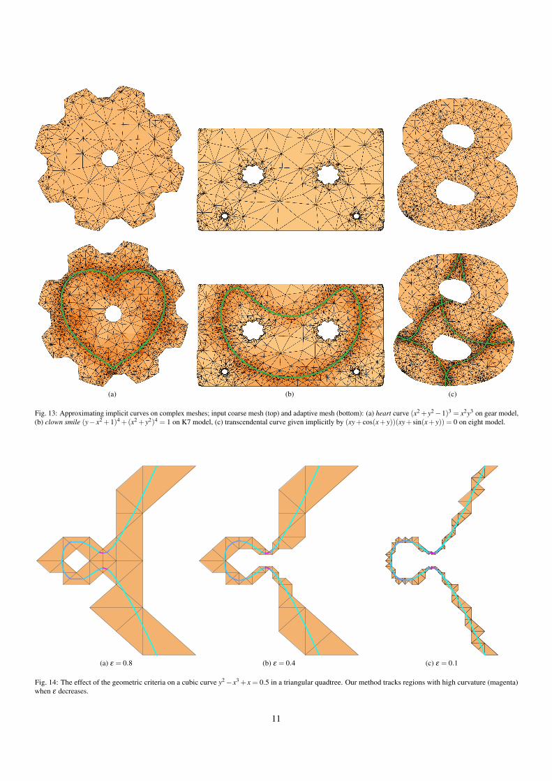
Fig. 12 shows that our method is able to approximate im-plicit curves on both convex and non-convex 4-8 meshes. Notehow our method tracks the main features of the curves, such assingularities and multiple components. Fig. 13 shows that ourmethod approximates nicely both algebraic and non-algebraiccurves on complex meshes for regions of arbitrary genus.

Fig. 14 illustrates the effect of the geometric criteria in ourmethod. This strategy produces well-adapted curves controlledby the tolerance ε (see Table 3), the only user-supplied parameterof our method. In order to demonstrate the efficiency of thegeometric criteria, the curvature is computed analytically andcolor coded from low (cyan) to high (magenta) absolute valuesof the curvature. Fig. 14 also shows how the mesh concentrateson high-curvature regions as we decrease ε .

Fig. 15 shows that our method adapts to the topology of thecurve using a small set of triangles. This adaptability cannotbe accomplished directly by the marching triangles algorithm.Indeed, the correct topology is reproduced by the marchingtriangles algorithm only after substantially refining the mesh,which significantly increases the number of triangles.

Fig. 16 shows that our method is able to approximate implicitcurves on a wide variety of triangulated surfaces, from closedsurfaces with or without boundary to surfaces with complextopology. Although finding an implicit curve on a triangulatedsurface S is equivalent to intersecting an implicit surface with S,our method does not need to triangulate the implicit surfaceand then intersect that mesh with S, a costly and potentiallynumerically delicate task.

The nodal domains (zero sets) of the real spherical harmon-ics Y k

4 of degree 4 and order k on the unit sphere (see Table 2) aregracefully approximated using our method, as shown in Fig. 17.The heavy refinement seen in the figure is due to the presence ofself-intersections in the curves.

Fig. 18 shows the intersection of a cylinder given implicitlywith a mesh of the unit sphere. The topology of the intersectioncurve varies with the position of the cylinder. Fig. 19 shows theintersection of a hyperboloid given implicitly with a Klein bottlesurface given parametrically. For comparison, the intersectionis found both on a mesh of the surface and directly on the para-metric domain. These two examples illustrate how our methodwould work for finding both intersection curves in space andtrimming curves in parametric space in a hybrid CSG modelingsystem that mixed implicit surfaces, parametric surfaces, andtriangle meshes.

All results were generated on a 2.4 GHz Intel Core i7 with8GB of RAM. Table 3 shows performance data, timings, andstatistics for these computations.

7. Conclusion

Like the method of Lopes et al. [5], our method computespolygonal approximations of implicit curves that are both spa-tially and geometrically adaptive. Unlike their method, however,our method does not need to compute derivatives because AAprovides second-order approximations. Moreover, our methodworks for both rectangular and triangular decompositions, struc-tured and unstructured, on the plane or on surfaces. It can use any

7

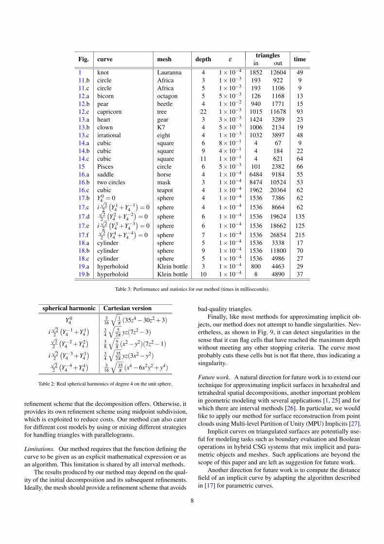
Fig. curve mesh depth εtriangles timein out

1 knot Lauranna 4 1×10−4 1852 12604 4911.b circle Africa 3 1×10−3 193 922 911.c circle Africa 5 1×10−3 193 1106 912.a bicorn octagon 5 5×10−3 126 1168 1312.b pear beetle 4 1×10−2 940 1771 1512.c capricorn tree 22 1×10−3 1015 11678 9313.a heart gear 3 3×10−3 1424 3289 2313.b clown K7 4 5×10−3 1006 2134 1913.c irrational eight 4 1×10−3 1032 3897 4814.a cubic square 6 8×10−1 4 67 914.b cubic square 9 4×10−1 4 184 2214.c cubic square 11 1×10−1 4 621 6415 Pisces circle 6 5×10−3 101 2382 6616.a saddle horse 4 1×10−4 6484 9184 5516.b two circles mask 3 1×10−4 8474 10524 5316.c cubic teapot 4 1×10−4 1962 20364 6217.b Y 0

4 = 0 sphere 4 1×10−4 1536 7386 6217.c i

√2

2

(Y 1

4 +Y−14

)= 0 sphere 4 1×10−4 1536 8664 62

17.d√

22

(Y 2

4 +Y−24

)= 0 sphere 6 1×10−4 1536 19624 135

17.e i√

22

(Y 3

4 +Y−34

)= 0 sphere 6 1×10−4 1536 18662 125

17.f√

22

(Y 4

4 +Y−44

)= 0 sphere 7 1×10−4 1536 26854 215

18.a cylinder sphere 5 1×10−4 1536 3338 1718.b cylinder sphere 9 1×10−4 1536 11800 7018.c cylinder sphere 5 1×10−4 1536 4986 2719.a hyperboloid Klein bottle 3 1×10−4 800 4463 2919.b hyperboloid Klein bottle 10 1×10−4 8 4890 37

Table 3: Performance and statistics for our method (times in milliseconds).

spherical harmonic Cartesian version

Y 04

316

√1π(35z4−30z2 +3)

i√

22

(Y−1

4 +Y 14) 3

4

√5

2πyz(7z2−3)

√2

2

(Y−2

4 +Y 24) 3

8

√5π(x2− y2)(7z2−1)

i√

22

(Y−3

4 +Y 34) 3

4

√352π

yz(3x2− y2)√

22

(Y−4

4 +Y 44) 3

16

√35π(x4−6x2y2 + y4)

Table 2: Real spherical harmonics of degree 4 on the unit sphere.

refinement scheme that the decomposition offers. Otherwise, itprovides its own refinement scheme using midpoint subdivision,which is exploited to reduce costs. Our method can also caterfor different cost models by using or mixing different strategiesfor handling triangles with parallelograms.

Limitations. Our method requires that the function defining thecurve to be given as an explicit mathematical expression or asan algorithm. This limitation is shared by all interval methods.

The results produced by our method may depend on the qual-ity of the initial decomposition and its subsequent refinements.Ideally, the mesh should provide a refinement scheme that avoids

bad-quality triangles.Finally, like most methods for approximating implicit ob-

jects, our method does not attempt to handle singularities. Nev-ertheless, as shown in Fig. 9, it can detect singularities in thesense that it can flag cells that have reached the maximum depthwithout meeting any other stopping criteria. The curve mostprobably cuts these cells but is not flat there, thus indicating asingularity.

Future work. A natural direction for future work is to extend ourtechnique for approximating implicit surfaces in hexahedral andtetrahedral spatial decompositions, another important problemin geometric modeling with several applications [1, 25] and forwhich there are interval methods [26]. In particular, we wouldlike to apply our method for surface reconstruction from pointclouds using Multi-level Partition of Unity (MPU) Implicits [27].

Implicit curves on triangulated surfaces are potentially use-ful for modeling tasks such as boundary evaluation and Booleanoperations in hybrid CSG systems that mix implicit and para-metric objects and meshes. Such applications are beyond thescope of this paper and are left as suggestion for future work.

Another direction for future work is to compute the distancefield of an implicit curve by adapting the algorithm describedin [17] for parametric curves.

8

Fig. 9: Our method detects the non-manifold region (red) in Tschirnhausen cubiccurve y2 = x3 + 3x2 on trapezoid, even when the singularity is not recovered(top right zoom).

Our method can be applied to parallelogram decompositionsof the plane, including the interesting Penrose tiling of Fig. 10.Penrose tilings with parallelograms admit a global refinementscheme but not a local one, and so cannot be used with ouradaptive method. Except for the midpoint subdivision scheme,we do not know any method for decomposing a parallelograminto smaller parallelograms. It would be interesting to find one. 10/10/13 2:41 PM

Page 1 of 1file:///Users/lhf/Desktop/Work/papers/CAG2013/penrose/w.svg

Fig. 10: Penrose tiling with parallelograms (source: Wikipedia).

Acknowledgments. A previous version of this paper was presented atSIBGRAPI 2012 [6]. The authors are partially supported by CNPq andFAPESP. This work was done in the Visgraf laboratory at IMPA, whichis sponsored by CNPq, FAPERJ, FINEP, and IBM Brasil.

References

[1] Patrikalakis NM, Maekawa T. Shape interrogation for computer aideddesign and manufacturing. Springer-Verlag; 2002.

[2] Moore RE. Interval Analysis. Prentice-Hall; 1966.[3] Moore RE, Kearfott RB, Cloud MJ. Introduction to Interval Analysis.

SIAM; 2009.[4] de Figueiredo LH, Stolfi J. Affine arithmetic: Concepts and applications.

Numerical Algorithms 2004;37(1):147–58.[5] Lopes H, Oliveira JB, de Figueiredo LH. Robust adaptive polygonal

approximation of implicit curves. Computers & Graphics 2002;26(6):841–52.

[6] Paiva A, de Carvalho Nascimento F, de Figueiredo LH, Stolfi J. Ap-proximating implicit curves on triangulations with affine arithmetic. In:Proceedings of SIBGRAPI 2012. IEEE Press; 2012, p. 94–101.

[7] Dobkin DP, Levy SVF, Thurston WP, Wilks AR. Contour tracing by piece-wise linear approximations. ACM Transactions on Graphics 1990;9(4):389–423.

[8] Persiano RCM, Comba JLD, Barbalho V. An adaptive triangulationrefinement scheme and construction. In: Proceedings of SIBGRAPI’93.1993, p. 259–66.

[9] Suffern KG, Fackerell ED. Interval methods in computer graphics. Com-puters & Graphics 1991;15(3):331–40.

[10] Mitchell DP. Three applications of interval analysis in computer graphics.In: Frontiers in Rendering course notes. SIGGRAPH’91; 1991, p. 14–1–14–13.

[11] Snyder JM. Interval analysis for computer graphics. Computer Graphics1992;26(2):121–30. (SIGGRAPH’92 Proceedings).

[12] Snyder JM. Generative Modeling for Computer Graphics and CAD. Aca-demic Press; 1992.

[13] Comba JLD, Stolfi J. Affine arithmetic and its applications to computergraphics. In: Proceedings of SIBGRAPI’93. 1993, p. 9–18.

[14] de Figueiredo LH, Stolfi J. Adaptive enumeration of implicit surfaces withaffine arithmetic. Computer Graphics Forum 1996;15(5):287–96.

[15] Martin R, Shou H, Voiculescu I, Bowyer A, Wang G. Comparison ofinterval methods for plotting algebraic curves. Computer Aided GeometricDesign 2002;19(7):553–87.

[16] de Cusatis Jr. A, de Figueiredo LH, Gattass M. Interval methods forray casting implicit surfaces with affine arithmetic. In: Proceedings ofSIBGRAPI’99. IEEE Press; 1999, p. 65–71.

[17] de Figueiredo LH, Stolfi J, Velho L. Approximating parametric curveswith strip trees using affine arithmetic. Computer Graphics Forum2003;22(2):171–9.

[18] Buhler K. Fast and reliable plotting of implicit curves. In: UncertaintyGeometric Computations. Kluwer Academic; 2002, p. 15–28.

[19] Buhler K. Implicit linear interval estimations. In: Proceedings of SCCG’02. ACM; 2002, p. 123–32.

[20] Stolfi J, de Figueiredo LH. Self-Validated Numerical Methods and Appli-cations. 21st Brazilian Mathematics Colloquium, IMPA; 1997.

[21] Gay O, Coeurjolly D, Hurstand N. Libaffa, C++ affine arithmetic library.2006. http://www.nongnu.org/libaffa/.

[22] Taubin G. Rasterizing algebraic curves and surfaces. IEEE ComputerGraphics and Applications 1994;14(2):14–23.

[23] Velho L, Zorin D. 4-8 subdivision. Computer-Aided Geometric Design2001;18(5):397–427.

[24] Kobbelt L.√

3-subdivision. In: Proceedings of SIGGRAPH ’00. ACM;2000, p. 103–12.

[25] Gomes A, Voiculescu I, Jorge J, Wyvill B, Galbraith C. Implicit Curvesand Surfaces: Mathematics, Data Structures and Algorithms. Springer;2009.

[26] Paiva A, Lopes H, Lewiner T, de Figueiredo LH. Robust adaptive meshesfor implicit surfaces. In: Proceedings of SIBGRAPI 2006. IEEE Press;2006, p. 205–12.

[27] Ohtake Y, Belyaev A, Alexa M, Turk G, Seidel HP. Multi-level partitionof unity implicits. ACM Transactions on Graphics 2003;22(3):463–70.(SIGGRAPH’03 Proceedings).

9

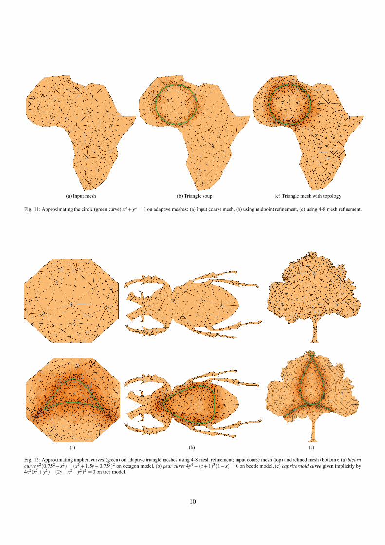
(a) Input mesh (b) Triangle soup (c) Triangle mesh with topology

Fig. 11: Approximating the circle (green curve) x2 + y2 = 1 on adaptive meshes: (a) input coarse mesh, (b) using midpoint refinement, (c) using 4-8 mesh refinement.

(a) (b) (c)

Fig. 12: Approximating implicit curves (green) on adaptive triangle meshes using 4-8 mesh refinement; input coarse mesh (top) and refined mesh (bottom): (a) bicorncurve y2(0.752− x2) = (x2 +1.5y−0.752)2 on octagon model, (b) pear curve 4y4− (x+1)3(1− x) = 0 on beetle model, (c) capricornoid curve given implicitly by4x2(x2 + y2)− (2y− x2− y2)2 = 0 on tree model.

10

(a) (b) (c)

Fig. 13: Approximating implicit curves on complex meshes; input coarse mesh (top) and adaptive mesh (bottom): (a) heart curve (x2 +y2−1)3 = x2y3 on gear model,(b) clown smile (y− x2 +1)4 +(x2 + y2)4 = 1 on K7 model, (c) transcendental curve given implicitly by (xy+ cos(x+ y))(xy+ sin(x+ y)) = 0 on eight model.

(a) ε = 0.8 (b) ε = 0.4 (c) ε = 0.1

Fig. 14: The effect of the geometric criteria on a cubic curve y2− x3 + x = 0.5 in a triangular quadtree. Our method tracks regions with high curvature (magenta)when ε decreases.

11

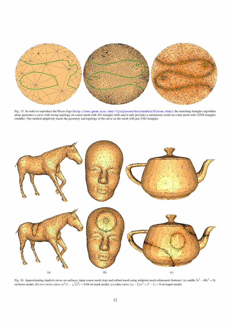
Fig. 15: In order to reproduce the Pisces logo (http://www.geom.uiuc.edu/~fjw/pisces/docs/models/Pisces.html), the marching triangles algorithmalone generates a curve with wrong topology on coarse mesh with 101 triangles (left) and it only provides a satisfactory result on a fine mesh with 12928 triangles(middle). Our method adaptively tracks the geometry and topology of the curve on the mesh with just 2382 triangles.

(a) (b) (c)

Fig. 16: Approximating implicit curves on surfaces; input coarse mesh (top) and refined mesh using midpoint mesh refinement (bottom): (a) saddle 3x2−48y2 = 8zon horse model, (b) two circles curve xy2(1−

√xy2) = 0.04 on mask model, (c) cubic curve (xy−2)(x2 + y2−1) = 0 on teapot model.

12

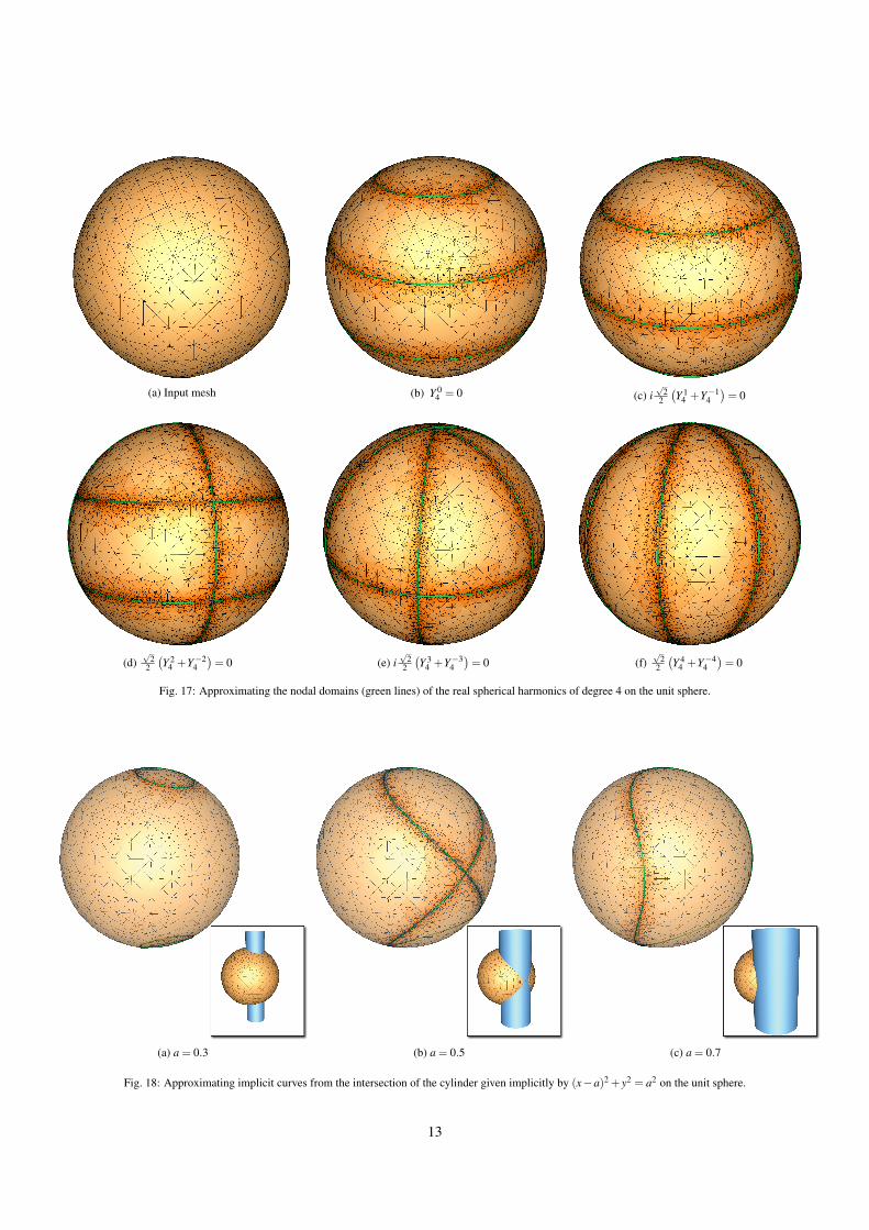
(a) Input mesh (b) Y 04 = 0 (c) i

√2

2

(Y 1

4 +Y−14)= 0

(d)√

22

(Y 2

4 +Y−24)= 0 (e) i

√2

2

(Y 3

4 +Y−34)= 0 (f)

√2

2

(Y 4

4 +Y−44)= 0

Fig. 17: Approximating the nodal domains (green lines) of the real spherical harmonics of degree 4 on the unit sphere.

(a) a = 0.3 (b) a = 0.5 (c) a = 0.7

Fig. 18: Approximating implicit curves from the intersection of the cylinder given implicitly by (x−a)2 + y2 = a2 on the unit sphere.

13

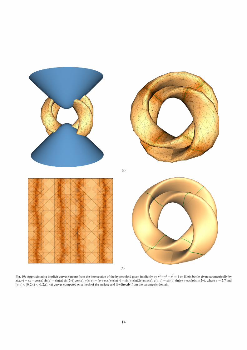
(a)

(b)

Fig. 19: Approximating implicit curves (green) from the intersection of the hyperboloid given implicitly by x2− y2− z2 = 1 on Klein bottle given parametrically byx(u,v) = (a+ cos(u)sin(v)− sin(u)sin(2v))cos(u), y(u,v) = (a+ cos(u)sin(v)− sin(u)sin(2v))sin(u), z(u,v) = sin(u)sin(v)+ cos(u)sin(2v), where a = 2.7 and(u,v) ∈ [0,2π)× [0,2π): (a) curves computed on a mesh of the surface and (b) directly from the parametric domain.

14