Optimal Regularization Parameter of the Multichannel Filtered-x Affine Projection Algorithm

4882 IEEE TRANSACTIONS ON SIGNAL PROCESSING, VOL. 55, NO. 10, OCTOBER 2007

Optimal Regularization Parameter of the MultichannelFiltered-x Affine Projection Algorithm

Alberto Carini, Senior Member, IEEE, and Giovanni L. Sicuranza, Life Senior Member, IEEE

Abstract—We discuss the optimal regularization parameter ofthe Filtered- Affine Projection (FX-AP) algorithm suitable forfeedforward active noise control. While the original FX-AP algo-rithm always provides a biased estimate of the minimum-mean-square solution, we show that the optimal regularized FX-AP algo-rithm is capable to eliminate the bias of the asymptotic solution andthus that the regularization parameter can optimize both the con-vergence speed and the residual MSE of the algorithm. We derivesome expressions for the optimal regularization parameter, and wediscuss some heuristic estimations of the optimal regularization pa-rameter in practical conditions.

Index Terms—Active noise control, affine projection algorithm,multichannel adaptive filtering, optimal regularization parameter.

I. INTRODUCTION

MULTICHANNEL active noise controllers are basedon the destructive interference in given locations of

the noise produced by some primary noise sources and someinterfering signals generated by secondary sources driven byan adaptive controller [1], [2]. One of the most successfulmethodologies is based on the so-called feedforward methods,where some reference signals are measured in the proximity ofthe noise source. These signals, together with the error signalscaptured in the proximity of the zone to be silenced, are usedfor adapting the controller and for estimating the signals of thesecondary sources. Due to the strong correlations between thesignals involved and the long impulse response of the primaryand secondary acoustic paths, a slow convergence of the con-troller’s adaptation algorithm has been often observed [3]. Toimprove the convergence behavior of the active noise controller,different Filtered- Affine Projection (FX-AP) algorithms havebeen proposed in the literature [4]–[6] in place of the usualFiltered- LMS algorithm (FX-LMS) at the expense of a lim-ited increment of the computational complexity of the updates.Indeed, the affine projection (AP) algorithms are a familyof adaptive filters that can produce a good tradeoff betweenconvergence speed and computational complexity. In [6], thetransient and the steady-state behavior of the FX-AP algorithmswere analyzed, and it was proven that these algorithms do notconverge to the minimum-mean-square (MMS) solution of

Manuscript received July 11, 2006; revised February 6, 2007. The associateeditor coordinating the review of this manuscript and approving it for publica-tion was Prof. John J. Shynk. This work was supported by MIUR under GrantPRIN 2004092314.

A. Carini is with the Information Science and Technology Institute, Univer-sity of Urbino “Carlo Bo,” 61029 Urbino, Italy (e-mail: [email protected]).

G. L. Sicuranza is with the Department of Electrical, Electronic andComputer Engineering, University of Trieste, 34127 Trieste, Italy (e-mail:[email protected]).

Digital Object Identifier 10.1109/TSP.2007.896113

the active noise control problem but to a biased asymptoticsolution, which depends on the statistics of the input signals.

The transient and the steady-state behavior of the FX-AP al-gorithms can be controlled by acting on the step-size param-eter of the adaptive filter. By reducing the step-size parameter,we can reduce the steady-state excess mean-square error (MSE)and the mean-square deviation of the algorithm, but the con-vergence speed reduces as well. A classical approach proposedin the literature to meet these conflicting requirements is thatof the variable step-size parameter methods. In these methods,the step-size parameter is varied in accordance with the state ofthe adaptive filter and its distance from the steady-state condi-tion. Different criteria have been developed for estimating thisdistance and for controlling the step-size parameter. The instan-taneous squared-error [7], the squared autocorrelation of errorat adjacent time [8], the fourth-order cumulant of the instanta-neous error [9], the instantaneous squared-error multiplied withan input-norm-dependent regularization factor [10] have beenused for controlling the step-size parameter of the LMS andnormalized least-mean-squares (NLMS) algorithms. By mini-mizing at each iteration, the mean-square deviation of the adap-tive filter, an optimal step-size parameter was obtained in [11]for the NLMS algorithm, and in [12] for the AP algorithm.Many of these criteria could also be adapted to the variablestep-size parameter control of the FX-AP algorithm. Neverthe-less, we must point out that these methodologies do not affectthe asymptotic solution of the FX-AP algorithm, and thus theyare not able to reduce the algorithm bias. Indeed, as shown in[6], the asymptotic solution of the multichannel exact FX-APalgorithm is independent of the step-size parameter. Therefore,while an optimal step-size parameter applied to this algorithmcan simultaneously maximize its convergence speed and mini-mize the excess MSE with respect to the asymptotic solution, itcannot reach the minimum achievable steady-state MSE givenby the MMS solution.

A different approach for meeting the conflicting requirementsof fast convergence and low steady-state error was recently pro-posed in the literature, and it is based on the concept of the op-timal regularization parameter [13]–[16]. In the AP algorithms,a regularization parameter is generally added to the decorrela-tion matrix to avoid its singularity in presence of highly corre-lated inputs. It was proven in [14] that the use of a regularizationparameter makes the AP algorithm more robust to both pertur-bations and model uncertainties. By acting on the regularizationparameter, it is possible to control the convergence speed, thesteady-state excess MSE, and the mean-square deviation of thealgorithm. A first expression of a pseudo-optimal regularizationparameter for AP algorithms was developed in [13]. White inputdata or prewhitened input data were considered, and the delay

1053-587X/$25.00 © 2007 IEEE

CARINI AND SICURANZA: OPTIMAL REGULARIZATION PARAMETER OF THE MULTICHANNEL FX-AP ALGORITHM 4883

Fig. 1. Schematic description of a multichannel feed-forward active noise control.

coefficient method [11] was used for estimating the system mis-match. Another method for the optimal choice of the regular-ization parameter was proposed in [14]. It requires again theestimation of the system mismatch, and it was derived by as-suming a particular form of the autocorrelation of the weighterror correlation matrix. More recently, in [15], an expressionof the optimal regularization parameter that employs only easilymeasurable quantities is presented. This expression is exact forwhite inputs or highly correlated inputs generated by processinga white input with a first-order autoregressive process. A gra-dient search of the optimal regularization parameter was alsoproposed in [16].

While the contributions about regularization presented in theliterature refer only to AP algorithms, in this paper we discussthe optimal regularization parameter of FX-AP algorithms. Weshow that, in contrast to the optimal variable step-size param-eter methods, the optimal regularization parameter can elimi-nate the bias of the asymptotic solution so that it is possibleto optimize both the convergence speed and the residual MSE.Following an approach similar to [15], we derive expressionsfor the exact and approximate optimal regularization parameter,and we discuss their heuristic estimation in practical conditions.For generality purposes, all results we provide refer to the mul-tichannel FX-AP algorithm, but the same results apply to thesingle-channel FX-AP.

The paper is organized as follows. Section II presents thestructure of the controller adopted in the paper and introducesthe multichannel exact FX-AP algorithm. Section III discussesthe asymptotic solution of the FX-AP algorithm and the effectof the regularization parameter on the bias. In Section IV, theoptimal regularization parameter value of the FX-AP algorithmis derived, and its estimation is discussed. Section V providessome experimental results in support of the proposed regular-

ization strategies. Some concluding remarks are provided inSection VI.

Throughout the paper, small boldface letters are used to de-note vectors, and bold capital letters are used to denote matrices,e.g., and , and all vectors are column vectors. The followingnotation is used:

indicates an identity matrix of appropriatedimensions;denotes the linear convolution;

is a block-diagonal matrix of the entries ;

denotes the mathematical expectation;

is the Euclidean norm;

is the trace of a matrix;

indicates the th eigenvalue of a matrix.

II. MULTICHANNEL FILTERED- AFFINE

PROJECTION ALGORITHM

A graphical description of a multichannel feedforward ac-tive noise control is shown in Fig. 1. reference sensors col-lect the corresponding input signals from the noise sources, and

error sensors collect the error signals at the interference lo-cations. The controller employs the signals coming from thesesensors in order to adaptively estimate output signals that feed

actuators.The corresponding block diagram is reported in Fig. 2. The

propagation of the original noise up to the region to be silencedis described by appropriate transfer functions character-izing the primary paths. The secondary noise signals propagatethrough secondary paths, which are represented by the transferfunctions , and we assume that there is no feedback be-


Fig. 2. Block diagram of delay-compensated filtered-x structure for active noise control.

tween the loudspeakers and the reference sensors. The primarysource signals filtered by the impulse responses of the secondarypath model, with transfer functions , are used for theadaptive filter update, and therefore the adaptation algorithmis called filtered- . Fig. 2 illustrates also the delay-compensa-tion scheme that is adopted throughout the paper [17]. To com-pensate for the propagation delay introduced by the secondarypaths, the output of the primary paths is estimated by sub-tracting the output of the secondary path model from the errorsensors signals .

Preliminary and independent evaluations of the secondarypath transfer functions are needed. In what follows, for sim-plicity sake, we work in the hypothesis of a perfect modelingof the secondary paths, i.e., we assume forany choice of and . When necessary, we will comment onthe different behavior of the system under perfect and imperfectestimations of the secondary paths.

We assume that any reference input of the adaptive controlleris connected with any actuator output through a filter whoseoutput depends linearly on the filter coefficients. Specifically,we assume that the th actuator output is given by the vectorequation

(1)

where is the coefficient vector of the filter that connectsthe input to the output of the adaptive controller, andis the th primary source input signal vector, which is a vectorfunction of the signal samples of th input. Its generalform is given by

(2)

where , for any is a time-invariant functional ofits argument. Equations (1) and (2) include linear filters, trun-cated Volterra filters of any order [18], radial basis functionnetworks [19], filters based on functional expansions [20] andother nonlinear filter structures. In Section V, we provide ex-perimental results both for linear filters, where the vectorreduces to

(3)

and for truncated second-order Volterra filters, where the inputdata vector is a collection of samples and of product ofsamples of the reference input . In this latter case,is given by

(4)

where is the memory length of the linear kernel, is thememory length of the quadratic kernel, and is the number ofimplemented diagonals of the quadratic kernel [18].

In this paper, we consider the multichannel exact FX-AP al-gorithm of [5] and [6]. To introduce this algorithm, we makeuse of quantities defined in Table I. The adaptation rule of thealgorithm can be expressed as follows:

(5)

where is the positive regularization parameter, and the matrixis a diagonal step-size matrix of appropriate dimensions.

III. ASYMPTOTIC SOLUTION AND REGULARIZATION

When the FX-AP algorithm is convergent the coefficientvector tends for to the asymptotic solution . The


TABLE IQUANTITIES USED FOR THE ALGORITHM DEFINITION

asymptotic solution can be estimated by manipulating (5). Bysubstituting the expression of of Table I in (5), we obtainthe expression

(6)

where

(7)

and

(8)

If we take the expectation of (6) and we consider the fixedpoint of the resulting equation, it can be easily deduced that theFX-AP algorithm, when converging, tends asymptotically to thecoefficient vector of

(9)

As discussed in [6], the asymptotic solution of the FX-AP algo-rithm is different from the MMS solution of the active noise con-trol problem, which minimizes the expectation of the residualsquare error. The MMS solution is given by [21]

(10)

where and are defined, respectively, as follows:

(11)

(12)

It is important to observe that the expression of the asymptoticsolution in (9) does not depend on the step-size matrix . There-fore, by varying the step-size parameter, as in optimal step-size


parameter algorithms, it is not possible to reduce the bias of theasymptotic solution. On the contrary, by acting on the regular-ization parameter, the algorithm can converge to the MMS so-lution of the active noise control problem. Indeed, we prove inthe Appendix that when , the asymptotic solution in(9) converges to . This result is in accordance with the factthat for the FX-AP algorithm tends to be an averagedFX-LMS algorithm. The FX-LMS algorithm, in the hypothesisof a perfect estimate of the secondary path, tends to the MMSsolution of the active noise control problem [22], [23]. Underimperfect estimate of the secondary paths, it was proved in theliterature that for a zero mean random estimation (like in on-lineestimation methods of the secondary paths) the FX-LMS algo-rithm converges to [22], [23], while a steady-state bias isoriginated by deterministic errors in the secondary path (likethose of off-line estimations of the secondary paths) [23]. Thesame considerations apply to the FX-AP algorithm when weconsider .

We will show in the next section that, in presence of stationaryinput signals, the optimal regularization parameter tends to be-come very large. Thus, in contrast to the original FX-AP algo-rithm, the optimal regularized FX-AP algorithm is only mar-ginally affected by a steady-state bias, and the residual MSE isoptimized.

IV. OPTIMAL REGULARIZATION PARAMETER

A. Exact Optimal Regularization Parameter

In this section, by following the approach of [15], we derivethe optimal regularization parameter of the FX-AP algorithm.Since we want to control the convergence and the steady-statebehavior of the FX-AP algorithm through the regularization pa-rameter, in (5) we set [13], [15], and we consider a timevarying regularization parameter. With these modifications, (5)can be rewritten as follows:

(13)

with

(14)

By using the results of [6], it can be proven that, in the hy-pothesis of a perfect estimation of the secondary paths, the al-gorithm in (13) is stable in the mean and mean-square sense.On the contrary, large estimation errors in the secondary pathscan lead to the instability of the algorithm for any possible valueof . This is the same behavior observed in the literature forother FX-LMS algorithms, which can become unstable for anypossible value of the step-size parameter [24].

The optimal regularization parameter is defined as thethat maximizes the reduction of the expectation of the

system distance, i.e.,

(15)

where the system error is defined as

(16)

By subtracting from both sides of (13), the following equa-tion is obtained:

(17)

from which it is immediate to compute the variation of the ex-pectation of the system distance at time :

(18)

The optimal regularization parameter can be obtained by set-ting to zero the derivative with respect to of system distancein (18). Before applying the derivative, we manipulate (18) inorder to derive a more tractable equation.

We define the optimal residual error

(19)

and the a priori error undistorted by the residual noise [25]

(20)

which are related to the following equation:

(21)

By introducing (20) and (21) in (18), we obtain the followingequation:

(22)

We perform the spectral decomposition of the matrix, which is given by

(23)

with the diagonal matrix formed by the eigenvalues of, i.e., , and with

the matrix formed by the eigenvectors of .can now be expressed as

(24)

and by substituting (23) and (24) in (22), we eventually get

(25)


By setting to zero the derivative of (25) with respect toand taking into account the expression of , it is proventhat the optimal regularization parameter meets the followingequation:

(26)

B. Approximate Optimal Regularization Parameter

Equation (26) has been obtained without resorting to any ap-proximation. Nevertheless, its solution requires the knowledgeof the spectral decomposition of the matrix , andtherefore it is not possible to derive a closed expression forwithout introducing some simplifying assumption. In particular,we introduce an approximation equivalent to that performed in[13] and [15], and we assume

(27)

This is a really strong approximation. However, it has beenshown in [15] that with standard AP algorithms, this kind ofapproximation leads to an expression for the regularization pa-rameter that can be also derived within different assumptionsthat hold for filters that are very long with respect to the AP order

. This fact is actually proven in two extreme cases, i.e., for awhite input (which is also the condition considered in [13]) or ifthe input is a highly correlated first-order autoregressive processwith pole close to 1. In FX-AP algorithms, the condition in (27)is surely met if the vectors are identically distributed anduncorrelated with each other and if we work with very long fil-ters (in these hypotheses, the matrix becomes adiagonal matrix with equal elements), but these conditions arenever verified in multichannel active noise controllers. Never-theless, the approximation in (27) allows us to derive usefulclosed expressions for . As shown in Section V, such ex-pressions provide interesting results for input signals modeledas a white predictable nonlinear process or, alternatively, as acombination of sinusoidal tones. In fact, by introducing the ap-proximation of (27) in (26) and by simplifying, we obtain thefollowing expression for :

(28)

By introducing (21) in (28), we can also rewrite in thefollowing alternative form:

(29)

It should be noticed that, apart from the different defini-tions of the involved quantities, the expression ofin (28) is equivalent to that in [15], and the expres-sion in (29) is formally equivalent to that in [13]. Themain difference is that, in the multichannel active noisecontrol context, and

, while the equalities holdfor the AP algorithms with exact modeling of the unknownsystem. Indeed, most multichannel active noise controllers do

not have an exact solution [26] but only an MMS solution.Therefore, in FX-AP algorithms, the optimal residual noise

does not coincide with the measurement noise, as forthe AP algorithms. Nevertheless, if we introduce the commonhypothesis that is uncorrelated with [6], [23],and if we take into account the orthogonality principle, itcan be proven that and

, and in this case the rela-tions in (28) and (29) become formally identical to those in[15] and [13], respectively. However, it should be noted that,while in our experiments with broadband noises the hypothesisof being uncorrelated with has been proven quiteaccurate, the same hypothesis has been proven false withmultitonal periodic noises.

Eventually, in the hypothesis that is uncorrelated withand that (which is the same

hypothesis introduced in [14]), the following alternative expres-sion for can be proven:

(30)

The relation in (30) is formally equivalent to that derived in [14].When the algorithm is convergent, we see that in the optimal

regularization parameters of (28), (29), and (30), the denomi-nator tends to reduce and consequently tends to becomevery large, thus eliminating the asymptotic bias of the FX-APalgorithm.

C. Heuristic Approximations of the OptimalRegularization Parameter

We now discuss some heuristic implementations of the op-timal regularization parameters of (28), (29), and (30).

The optimal regularization parameters in (29) and (30) re-quire the estimation of the system error , or of the systemdistance . In AP or LMS algorithms, the system distanceis typically evaluated with the delay coefficient technique [11].Unfortunately, this technique cannot be applied in active noisecontrollers. Indeed, the controller acts as a predictor of the inputsignals [19] and, even if we delay the error microphone signals,the optimal value of the first coefficients will never be zero.

The optimal regularization parameter in (28) is moretractable because it depends only on easily measurablepowers and on a cross-correlation measure. The terms

and can be estimated by exponentiallysmoothing the trace and the instantaneouspower . A more careful estimate is needed for thecross-correlation . If is uncorrelatedwith reduces to the optimal residualpower , which is a constant. Therefore, we canapproximate (28) with the following equation:

(31)

where the constant is an estimate of the residual power andis a small positive constant used to avoid negative values for thedenominator. Our experiments have confirmed that the perfor-mances obtained with (31) actually depend on the validity of thehypothesis of being uncorrelated with , and on thevalue of . If the hypothesis is verified and is smaller than the


TABLE IIEIGENVALUES OF E[U (n)U(n)] IN THE FIRST 50 000 SAMPLES OF EXPERIMENT 1 FOR AP ORDER L = 1, 3, AND 5

TABLE IIIEIGENVALUES OF E[U (n)U(n)] IN THE FIRST 50 000 SAMPLES OF EXPERIMENT 2 FOR AP ORDER L = 1; 3; AND 5

residual power, the asymptotic value of is upper boundedand the bias on the asymptotic solution is not eliminated (even ifit is surely reduced for large values). On the contrary, ifis larger than the residual power, the algorithm converges to theMMS solution but the convergence speed is noticeably reduced.

Another possibility is that of estimating the optimal residualpower with the lower envelope of theinstantaneous power , i.e., with a minima trackingtechnique, as follows [11], [27]:

ifif

(32)

with , and to approximate with

(33)

With this estimation, the asymptotic value of surely un-derestimates the optimal residual power and the regularized al-gorithm will not be able to completely eliminate the asymp-totic bias. Nevertheless, the regularization parameter in (33) hasprovided interesting results in our simulations also in the caseswhere is correlated to .

V. EXPERIMENTAL RESULTS

In this section, we provide some experimental results thatcompare the FX-AP algorithm equipped with the approximateregularization parameter of (28), with the heuristic regulariza-tion parameters of (31) and (33), and with fixed regularizationparameters.

In all regularization methods, we have adaptively estimatedand as follows:

(34)

(35)

and we have set the forgetting factor equal to 0.99.

In the optimal regularization parameter of (28), the errorhas been evaluated with the optimal coefficient vector

, which in each experiment has been a priori determinedwith (10). Then, the cross-correlation has beenevaluated by exponentially smoothing with a forgetting factor

the instantaneous products .In the regularization parameter of (31), the constant has

been set equal to the optimal residual error power, i.e.,with ,

and with defined in (11) and (12), respectively.In (31) and (33), the constant has been set equal to 0.01, and

the forgetting factors and for the estimation ofhave been set equal to 0.99 and 0.999, respectively.

A. Experiment 1

In the first experiment, we consider the same experimentalconditions of the Third Experiment of [6], i.e., we consider amultichannel active noise controller with .The input signal is the normalized logistic noise and thecontroller is a two-channel second-order Volterra filter withmemory length of the linear and quadratic part 4, i.e., with

, and one diagonal for the quadratic kernel, i.e.,with in (4). The transfer functions of the primary pathsare

(36)

(37)

and the transfer functions of the secondary paths are

(38)

(39)

(40)

(41)

In contrast to [6], in order to test the tracking behavior of theFX-AP algorithm, after 50 000 samples, we multiply the transferfunction of the primary paths by , while keeping constant thesecondary paths.

We first study the approximation of (27). Table II providesthe eigenvalues of in the first 50 000 samples ofExperiment 1 for AP order 1, 3, and 5. As we can see, theyare sparse and differ from the value provided by (27), which is


Fig. 3. Evolution of E[e (n)e (n)] of the FX-AP algorithm with the regu-larization parameter of (28) for AP order L = 1, 3, and 5.

50.74. Therefore, (28), (31), and (33) provide only suboptimalsolutions to the regularization problem.

Fig. 3 diagrams the estimated cross-correlation(divided by the AP order ) of the FX-AP

algorithm equipped with the regularization parameter of(28). Each point of Fig. 3 represents the ensemble average,estimated over 200 runs of the algorithm, of the mean valueof the cross-correlation computed on 100 successive samples.In the figure, the dashed line represents the optimal residualpower obtained with . As we can see, in this experiment, theestimated cross-correlation can be reasonably approximatedwith the optimal residual power, and therefore we expect thatthe regularization parameter in (31) should approximate wellthe regularization parameter of (28).

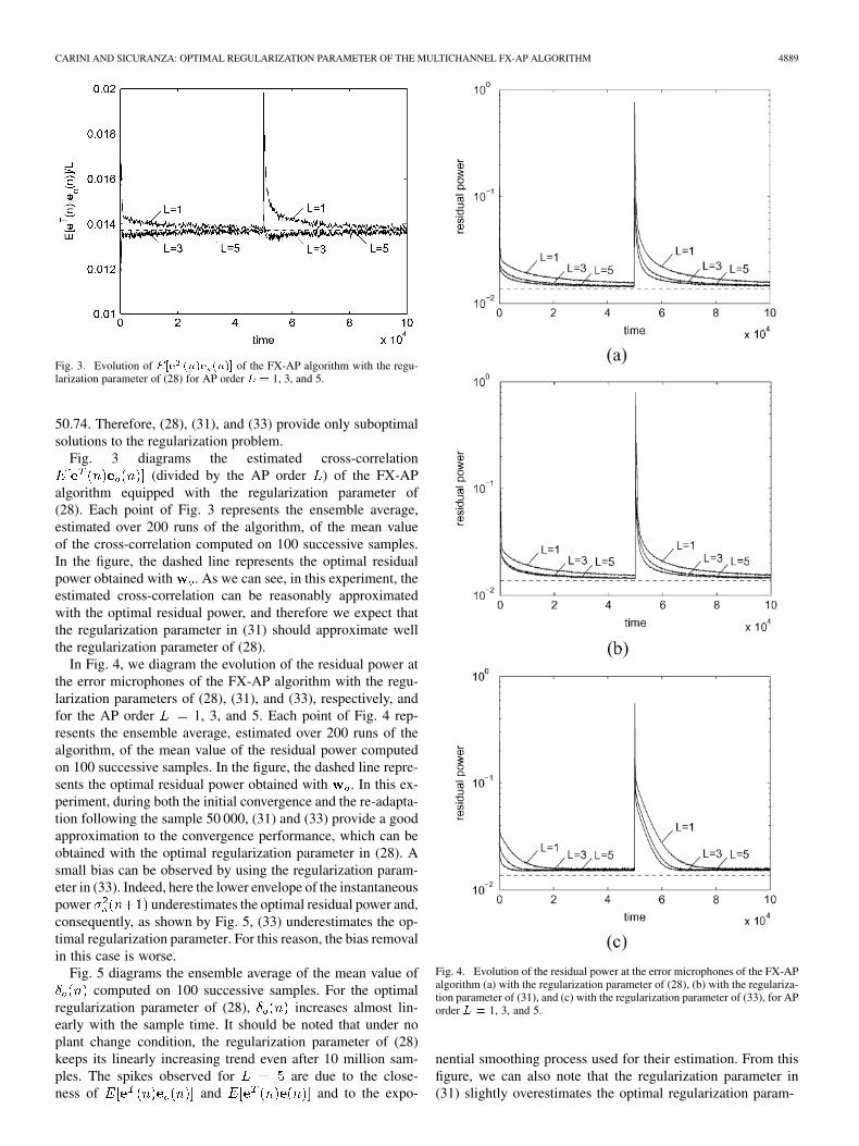
In Fig. 4, we diagram the evolution of the residual power atthe error microphones of the FX-AP algorithm with the regu-larization parameters of (28), (31), and (33), respectively, andfor the AP order 1, 3, and 5. Each point of Fig. 4 rep-resents the ensemble average, estimated over 200 runs of thealgorithm, of the mean value of the residual power computedon 100 successive samples. In the figure, the dashed line repre-sents the optimal residual power obtained with . In this ex-periment, during both the initial convergence and the re-adapta-tion following the sample 50 000, (31) and (33) provide a goodapproximation to the convergence performance, which can beobtained with the optimal regularization parameter in (28). Asmall bias can be observed by using the regularization param-eter in (33). Indeed, here the lower envelope of the instantaneouspower underestimates the optimal residual power and,consequently, as shown by Fig. 5, (33) underestimates the op-timal regularization parameter. For this reason, the bias removalin this case is worse.

Fig. 5 diagrams the ensemble average of the mean value ofcomputed on 100 successive samples. For the optimal

regularization parameter of (28), increases almost lin-early with the sample time. It should be noted that under noplant change condition, the regularization parameter of (28)keeps its linearly increasing trend even after 10 million sam-ples. The spikes observed for are due to the close-ness of and and to the expo-

Fig. 4. Evolution of the residual power at the error microphones of the FX-APalgorithm (a) with the regularization parameter of (28), (b) with the regulariza-tion parameter of (31), and (c) with the regularization parameter of (33), for APorder L = 1, 3, and 5.

nential smoothing process used for their estimation. From thisfigure, we can also note that the regularization parameter in(31) slightly overestimates the optimal regularization param-


Fig. 5. Evolution of (a) the regularization parameter of (28), (b) the reg-ularization parameter of (31), and (c) the regularization parameter of (33),for AP order L = 1, 3, and 5.

eter of (28), but the overestimation here does not affect appre-ciably the convergence of the algorithm. Nevertheless, under

no plant change condition, this tends to an asymptoticvalue after around 1 million samples. Eventually, note that thevertical scale of Fig. 5(c) has been reduced for better fittingthe curves.

For comparison purposes, Fig. 6 plots the evolution of theresidual power at the error microphones of the FX-AP algo-rithm with a small fixed regularization parameter equal to 0.001,as usually done to only avoid numerical instabilities and withstep-size parameter equal to 0.1, 0.01, and 0.001, respectively.From Fig. 6, it is apparent that, due to the algorithm bias, no ac-ceptable behavior can be obtained without introducing a suitablylarge regularization parameter. Fig. 7 plots the evolution of theresidual power at the error microphones of the FX-AP algorithmwith step-size parameter and a fixed regularization pa-rameter equal to , respectively.Fig. 7(b) provides the best compromise between convergencespeed and residual mean square error. Indeed, the performancesof the algorithm for are almost comparable to thoseobtained with the optimal regularization parameter. Neverthe-less, it should be noted that if we increase the simulation in-terval, the residual power of the AP algorithm equipped withthe optimal regularization parameter converges to the optimalresidual power. On the contrary, the algorithm with a fixed reg-ularization parameter reaches at most the asymptotic residualpower of Fig. 7(b).

B. Experiment 2

In the second experiment, we consider a multichannel activenoise controller with . The input signal isgiven by three sinusoids with unitary amplitude, random phase,and normalized frequencies and . Thethree sinusoids are corrupted with a white Gaussian noise until30 dB of signal-to-noise ratio (SNR). The primary and sec-ondary paths are realistic impulse responses with 100 taps. Oneof the primary paths and one of the secondary paths have beenobtained by truncating the impulse response of the acousticpaths reported in the companion disk of [2] for a single-channelactive noise controller. The other primary and secondary pathshave been obtained by adding exponentially decreasing randomnoises to the impulse response of the acoustic paths of [2].The exponentially decreasing random noises had a standarddeviation between the 20% and the 40% of the amplitude ofthe impulse response. The output of the primary paths has beencorrupted with a white Gaussian noise until 30 dB of SNR. Thecontroller is a two-channel linear filter with memory length 32.

Table III provides the eigenvalues of in thefirst 50 000 samples for AP order 1, 3, and 5. The eigen-values are even more sparse than in Experiment 1, and theydiffer considerably from the value provided by (27), which is1331.55. Therefore, (28), (31), and (33) provide a suboptimalsolution to the regularization problem.

Fig. 8 diagrams the estimated cross-correlation(divided by the AP order ) of the FX-AP

algorithm equipped with the regularization parameter of (28).Each point of Fig. 9 represents the ensemble average, estimatedover 200 runs of the algorithm, of the mean value of the cross-


Fig. 6. Evolution of the residual power at the error microphones of the FX-APalgorithm with a fixed regularization parameter � = 0:001 with (a) � = 0:1,(b) � = 0:01, and (c) � = 0:001 for AP order L = 1, 3, and 5.

correlation computed on 100 successive samples. In thefigure, the dashed line represents the optimal residual power

Fig. 7. Evolution of the residual power at the error microphones of the FX-APalgorithm with step-size parameter � = 1:0 and a fixed regularization param-eter equal to (a) � = 10:0, (b) � = 100:0, and (c) � = 1000:0 for AP orderL = 1, 3, and 5.

obtained with . As we can see, with tonal input noise theoptimal residual power differs from the cross-correlation


Fig. 8. Evolution of E[e (n)e (n)] of the FX-AP algorithm with the regu-larization parameter of (28) for AP order L = 1, 3, and 5.

. In this situation, the regularization parameterof (31) provides a rough estimate of the regularization parameterin (28).

In Fig. 9, we diagram the evolution of the residual power atthe error microphones of the FX-AP algorithm with the regular-ization parameters of (28), (31), and (33), and for the AP order

1, 3, and 5. Each point of Fig. 9 represents the ensembleaverage, estimated over 200 runs of the algorithm, of the meanvalue of the residual power computed on 100 successive sam-ples. Moreover, Fig. 10 diagrams the ensemble average of themean value of the corresponding computed on 100 suc-cessive samples. The vertical scale of the Fig. 10(b) has beenexpanded for fitting the curves.

Again, after the initial convergence, the optimal regular-ization parameter of (28) increases almost linearly with thesample time, and under no plant change condition keepsits linearly increasing trend even after 10 million samples. Inthis experiment, the regularization parameter in (33) providesa good approximation of the performance obtained with theoptimal regularization parameter in (28). Nevertheless, underno plant change condition, tends to an asymptotic valuein less than 1 million samples. In this experiment, (31) providesthe worst approximation of the optimal regularization param-eter. Indeed, as shown in Fig. 8, overestimates

and thus the regularization parameter in (31)tends to excessively overestimate the optimal regularizationparameter. As a consequence, the adaptation of the FX-APalgorithm is frozen before reaching the optimal MSE. Duringthe readaptation following the sample 50 000, the regular-ization parameters in (31) and (33) provide only a coarseapproximation of the performance of the optimal regularizedFX-AP algorithm thus indicating a suboptimal behavior. It isworth noting, however, that also the approximate regularizationparameter in (28) provides a suboptimal behavior during thesame readaptation, which is slower than the initial adaptation

Fig. 9. Evolution of the residual power at the error microphones of the FX-APalgorithm (a) with the regularization of (28), (b) with the regularization param-eter of (31), and (c) with the regularization parameter of (33), for AP orderL =1, 3, and 5.

after the sample 0. Indeed, we can argue that the approximationin (27) is excessively strong for tonal noise.


Fig. 10. Evolution of (a) the regularization parameter of (28), (b) the regular-ization parameter of (31), and (c) the regularization parameter of (33), for APorder L = 1, 3, and 5.

Fig. 11 plots the evolution of the residual power at the errormicrophones of the FX-AP algorithm with a small fixed regular-

Fig. 11. Evolution of the residual power at the error microphones of the FX-APalgorithm with a fixed regularization parameter � = 0:001 with (a) � = 1:0,(b) � = 0:1, and (c) � = 0:01 for AP order L = 1, 3, and 5.

ization parameter equal to 0.001 as usually done to only avoidnumerical instabilities and with step-size parameter equal to 1.0,


Fig. 12. Evolution of the residual power at the error microphones of the FX-APalgorithm with step-size parameter � = 1:0 and a fixed regularization param-eter equal to (a) � = 10:0, (b) � = 100:0, and (c) � = 1000:0 for AP orderL = 1, 3, and 5.

0.1, and 0.01, respectively. While for we have a rea-sonable compromise in terms of convergence speed and residualpower, the effect of the bias in the asymptotic solution is still ev-ident, especially for .

Fig. 12 plots the evolution of the residual power at the errormicrophones of the FX-AP algorithm with step-size parameter

and a fixed regularization parameter equal to, respectively. In this case, for

the initial performance of the algorithm is even betterthan those obtained in Fig. 9(a) with the optimal regularizationparameter in (28), thus showing the suboptimality of this solu-tion when the approximation in (27) is largely violated. Never-theless, we should note again that the algorithm equipped with afixed regularization parameter cannot reach the optimal residualpower. On the contrary, the residual power of the AP algorithmequipped with the optimal regularization parameter of (28) inthe long term converges to the optimal residual power.

VI. CONCLUSION

In this paper we have discussed the optimal regularization pa-rameter of the FX-AP algorithm. We have proved that, in con-trast to the FX-AP algorithm without regularization parameter,the optimal regularized algorithm is capable to converge to theMMS solution of the active noise control problem. We have de-rived exact, approximate and heuristic expressions for the op-timal regularization parameter and we have compared them withnumerical experiments. The experimental results show that theconvergence and tracking performances of the FX-AP algorithmcan be greatly improved through optimal regularization param-eter. Moreover, the proposed heuristic regularization parame-ters provide a reasonably good and efficient approximation ofthe optimal regularization parameter, even though there is stillroom for improvement in this estimation, especially for tonalinput noise.

APPENDIX

For the matrix inversion lemma

(42)

where is a term that, when , converges to zeroat least as fast as . Thus, for large values of , we have

(43)

and

(44)

In the hypothesis of stationary input signals, it is

(45)

and

(46)

By replacing (43)–(46) in (9) and taking into account (10), weprove that, when converges to .

REFERENCES

[1] P. A. Nelson and S. J. Elliott, Active Control of Sound. London, U.K.:Academic, 1995.

[2] S. M. Kuo and D. R. Morgan, Active Noise Control Systems-Algorithmsand DSP Implementation. New York: Wiley, 1996.


[3] S. C. Douglas, “Fast implementations of the filtered-X LMS and LMSalgorithms for multichannel active noise control,” IEEE Trans. SpeechAudio Process., vol. 7, pp. 454–465, Jul. 1999.

[4] S. C. Douglas, “The fast affine projection algorithm for active noisecontrol,” in Proc. 29th Asilomar Conf. Signals, Systems, Computers,Pacific Grove, CA, Nov. 1995, vol. 2, pp. 1245–1249.

[5] M. Bouchard, “Multichannel affine and fast affine projection algo-rithms for active noise control and acoustic equalization systems,”IEEE Trans. Speech Audio Process., vol. 11, no. 1, pp. 54–60, Jan.2003.

[6] A. Carini and G. L. Sicuranza, “Transient and steady-state analysis offiltered-X affine projection algorithms,” IEEE Trans. Signal Process.,vol. 54, no. 2, pp. 665–678, Feb. 2006.

[7] R. H. Kwong and E. W. Johnston, “A variable step size LMS algo-rithm,” IEEE Trans. Signal Process., vol. 40, pp. 1633–1642, Jul. 1992.

[8] T. Aboulnasr and K. Mayyas, “A robust variable step-size LMS-typealgorithm: Analysis and simulations,” IEEE Trans. Signal Process.,vol. 45, no. 3, pp. 631–639, Mar. 1997.

[9] D. I. Pazaitis and A. G. Constantinides, “A novel kurtosis driven vari-able step-size adaptive algorithm,” IEEE Trans. Signal Process., vol.47, no. 3, pp. 864–872, Mar. 1999.

[10] M. H. Costa and J. C. Bermudez, “A robust variable step size algorithmfor LMS adaptive filters,” in Proc. Int. Conf. Acoustics, Speech, SignalProcessing (ICASSP), Toulose, France, May 2006, pp. iii-93–iii-96.

[11] A. Mader, H. Puder, and G. U. Schmidt, “Step-size control for acousticecho cancellation filters—An overview,” Signal Process., vol. 4, pp.1697–1719, Sep. 2000.

[12] H.-C. Shin, A. H. Sayed, and W. J. Song, “Variable step-size NLMSand affine projection algorithms,” IEEE Signal Process. Lett., vol. 11,no. 2, pp. 132–135, Feb. 2004.

[13] V. Myllyla and G. Schmidt, “Pseudo-optimal regularization for affineprojection algorithms,” in Proc. Int. Conf. Acoustics, Speech, SignalProcessing (ICASSP) , Orlando, FL, May 2002, pp. 1917–1920.

[14] H. G. Rey, L. R. Vega, S. Tressens, and B. C. Frias, “Analysis of explicitregularization in affine projection algorithms: Robustness and optimalchoice,” in Proc. Eur. Signal Processing Conf. (EUSIPCO), Vienna,Austria, Sep. 2004, pp. 1089–1092.

[15] H. G. Rey, L. R. Vega, S. Tressens, and J. Benesty, “Optimum vari-able explicit regularized affine projection algorithm,” in Proc. Int. Conf.Acoustics, Speech, Signal Processing (ICASSP), Toulose, France, May2006, pp. iii-197–iii-200.

[16] Y. S. Choi, H.-C. Shin, and W. J. Song, “Affine projection algorithmswith adaptive regularization matrix,” in Proc. Int. Conf. Acoustics,Speech, Signal Processing (ICASSP), Toulose, France, May 2006, pp.iii-201–iii-204.

[17] M. Bouchard and S. Quednau, “Multichannel recursive least-squaresalgorithms and fast-transversal-filter algorithms for active noise controland sound reproduction systems,” IEEE Trans. Speech Audio Process.,vol. 8, no. 5, pp. 606–618, Sep. 2000.

[18] V. J. Mathews and G. L. Sicuranza, Polynomial Signal Processing.New York: Wiley, 2000.

[19] P. Strauch and B. Mulgrew, “Active control of nonlinear noise pro-cesses in a linear duct,” IEEE Trans. Signal Process., vol. 46, no. 9, pp.2404–2412, Sep. 1998.

[20] D. P. Das and G. Panda, “Active mitigation of nonlinear noise processesusing a novel filtered-s LMS algorithm,” IEEE Trans. Speech AudioProcess., vol. 12, no. 3, pp. 313–322, May 2004.

[21] S. J. Elliott, I. M. Stothers, and P. A. Nelson, “A multiple error LMSalgorithm and its application to the active control of sound and vibra-tion,” IEEE Trans. Acoustics, Speech, Signal Process., vol. ASSP-35,pp. 1423–1434, Oct. 1987.

[22] E. Bjarnason, “Analysis of the filtered-X LMS algorithm,” IEEE Trans.Speech Audio Process., vol. 3, no. 6, pp. 504–514, Nov. 1995.

[23] O. J. Tobias, J. C. M. Bermudez, and N. J. Bershad, “Mean weight be-havior of the filtered-X LMS algorithm,” IEEE Trans. Signal Process.,vol. 48, no. 4, pp. 1061–1075, Apr. 2000.

[24] S. D. Snyder and C. H. Hansen, “The effect of transfer function esti-mation errors on the filtered-X LMS algorithms,” IEEE Trans. SignalProcess., vol. 42, no. 4, pp. 950–953, Apr. 1994.

[25] H.-C. Shin and A. H. Sayed, “Mean-square performance of a family ofaffine projection algorithms,” IEEE Trans. Signal Process., vol. 52, no.1, pp. 90–102, Jan. 2004.

[26] M. Miyoshi and Y. Kaneda, “Inverse filtering of room acoustics,” IEEETrans. Signal Process., vol. 36, no. 2, pp. 145–152, Feb. 1988.

[27] P. Heitkämper, “An adaptation control for acoustic echo cancellers,” inIEEE Signal Process. Lett., vol. 80, pp. 170–172.

Alberto Carini (S’89–A’97–M’02–SM’06) wasborn in Trieste, Italy, in 1967. He received the Laureadegree (summa cum laude) in electronic engineeringand the Dottorato di Ricerca (Ph.D.) degree in infor-mation engineering from the University of Trieste,Italy, in 1994 and 1998, respectively.

In 1996 and 1997, during his doctoral studies, hewas a Visiting Scholar with the University of Utah,Salt Lake City. From 1997 to 2003, he was a DSPEngineer with Telit Mobile Terminals SpA, Trieste,Italy, where he led the audio processing research and

development activities. In 2003, he was with Neonseven srl, Trieste, Italy, as anaudio and DSP expert. From 2001 to 2004, he collaborated with the Universityof Trieste as a Contract Professor of digital signal processing. Since 2004, he hasbeen an Associate Professor with the Information Science and Technology In-stitute (ISTI), University of Urbino, Urbino, Italy. His research interests includeadaptive filtering, nonlinear filtering, nonlinear equalization, acoustic echo can-cellation, and active noise control.

Prof. Carini is a currently a member of the Editorial Board of Signal Pro-cessing, Elsevier, and a member of the SPTM Technical Committee of the IEEESignal Processing Society. He received the Zoldan Award for the best Laureadegree in electronic engineering at the University of Trieste for the AcademicYear 1992–1993.

Giovanni L. Sicuranza (M’73–SM’85–LSM’06)is Professor of signal and image processing at theDepartment of Elettrotecnica Elettronica Informatica(DEEI), University of Trieste, Italy, where he hasgiven courses on analog circuits, digital circuits, anddigital signal and image processing. He was also ateacher in European courses on image processingand analysis, and the organizer of the EURASIPcourse on Linear and Nonlinear Filtering of Multi-dimensional Signals (Trieste, Italy, 1990). At DEEI,he founded the Image Processing Laboratory in

1980 and was its director until 2005. He has published a number of papers ininternational journals and conference proceedings. He contributed chapters forseven books and is the coeditor with Prof. S. Mitra, University of Californiaat Santa Barbara, of the books Multidimensional Processing of Video Signals,(Norwell, MA: Kluwer Academic, 1992) and Nonlinear Image Processing(New York: Academic, 2001), and with Prof. S. Marshall, University ofStrathclyde, Glasgow, U.K., of the book Advances in Nonlinear Signal andImage Processing (New York: Hindawi Publishing Corp., 2006). He is thecoauthor with Prof V. J. Mathews, University of Utah at Salt Lake City, of thebook Polynomial Signal Processing (New York: Wiley, 2000). His researchinterests include multidimensional digital filters, polynomial filters, processingof images and image sequences, image coding, and adaptive algorithms forecho cancellation and active noise control.

Prof. Sicuranza has been a member of the technical committees of numerousinternational conferences; the Chairman of the VIII European Signal Pro-cessing Conference (EUSIPCO) 1996, Trieste, Italy, and the Sixth Workshopon Nonlinear Signal and Image Processing (NSIP) 2003, Grado, Italy; and theCo-Chair of the IEEE International Conference on Image Processing (ICIP)2005, Genova, Italy. He was a member of the Editorial Board of the EURASIPjournal Signal Processing and of the IEEE SIGNAL PROCESSING MAGAZINE.He is presently an Associate Editor of Multidimensional Systems and SignalProcessing and a member of the editorial board of the EURASIP book serieson Signal Processing and Communications. He has served as a project managerof ESPRIT and COST research projects funded by the European Commissionand as a consultant to several industries. He was the Awards Chairman ofthe Administrative Committee of EURASIP and a member of the IMDSPTechnical Committee of the IEEE Signal Processing Society. He has beenone of the founders and the first Chairman of the Nonlinear Signal and ImageProcessing (NSIP) Board of which he is still a member. In 2006, he receivedthe EURASIP Meritorious Service Award.

Optimal Regularization Parameter of the Multichannel Filtered-x Affine Projection Algorithm

Documents

Transcript of Optimal Regularization Parameter of the Multichannel Filtered-x Affine Projection Algorithm