Int J Comput VisDOI 10.1007/s11263-009-0205-5

A Study on Smoothing for Particle-Filtered 3D Human BodyTracking

Patrick Peursum · Svetha Venkatesh · Geoff West

Received: 11 January 2008 / Accepted: 6 January 2009© Springer Science+Business Media, LLC 2009

Abstract Stochastic models have become the dominantmeans of approaching the problem of articulated 3D humanbody tracking, where approximate inference is employedto tractably estimate the high-dimensional (∼30D) posturespace. Of these approximate inference techniques, particlefiltering is the most commonly used approach. However fil-tering only takes into account past observations—almostno body tracking research employs smoothing to improvethe filtered inference estimate, despite the fact that smooth-ing considers both past and future evidence and so shouldbe more accurate. In an effort to objectively determine theworth of existing smoothing algorithms when applied to hu-man body tracking, this paper investigates three approxi-mate smoothed-inference techniques: particle-filtered back-wards smoothing, variational approximation and Gibbs sam-pling. Results are quantitatively evaluated on both the HU-MANEVA dataset as well as a scene containing occludingclutter. Surprisingly, it is found that existing smoothing tech-niques are unable to provide much improvement on the fil-tered estimate, and possible reasons as to why are exploredand discussed.

Keywords Articulated human body tracking ·Particle filtering · Smoothing

P. Peursum (�) · S. Venkatesh · G. WestDept of Computing, Curtin University of Technology,GPO Box U1987, Perth, Western Australia, Australiae-mail: P.Peursum@curtin.edu.au

S. Venkateshe-mail: S.Venkatesh@curtin.edu.au

G. Weste-mail: G.West@curtin.edu.au

1 Introduction

In time-series data with noisy observations, filtering is theprocess of estimating (or tracking) the true state at time t

given all the observations {y1, . . . , yt } that lead up to t , andsmoothing is the process of using all future observations{yt+1, . . . , yT } to correct the filtering estimate in light ofthe future evidence. Consequently, smoothing should pro-vide a better estimate than filtering since it takes all availableevidence into account. Hence it is common practice to usesmoothed estimates in many fields such as signal processingand speech recognition. In contrast, research into articulatedhuman body tracking is dominated by filtering. In genera-tive (top-down) tracking where the observation is viewedas ‘caused’ by the true state, the most prevalent approachis particle filtering (Moeslund et al. 2006) which approxi-mates the state with a set of weighted Monte Carlo sam-ples called particles (Doucet et al. 2000). However, researchemploying smoothed inference for body tracking is almostnon-existent despite the existence of several smoothing al-gorithms for particle filters that have been shown to benefitother tracking fields (Doucet et al. 2002; Godsill et al. 2004;Klaas et al. 2006), as well as alternative efficient approxi-mate smoothed inference techniques such as variational andGibbs sampling (Ghahramani and Jordan 1997).

This paper investigates approximate smoothing tech-niques in order to ascertain their worth for 3D multi-viewarticulated human body tracking in both controlled and re-alistic environments, where the latter contains occludingobjects such as tables and chairs. Such realistic scenes arerarely considered in human body tracking since occlusionsproduce observation ‘errors’ and thus often cause filteredtracking to fail for the duration of the occlusion. Our previ-ous work (Peursum et al. 2007) showed that a strong motionmodel can minimise such failures, but this restricts tracking

Int J Comput Vis

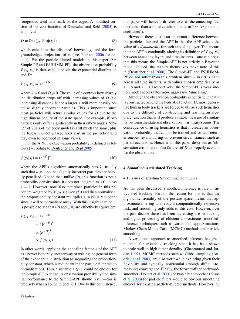
Fig. 1 Overview of the algorithms and data sets investigated in this paper. Both datasets are filtered with three filtering algorithms; each filteredresult is passed on to the three smoothing algorithms to produce nine smoothing results, which are evaluated along with the three filtering results

to modelled motions. In contrast, smoothing is applicableto any motion dynamics and has been reported to improvetracking estimates over filtering in other, lower-dimensional,tracking fields (Doucet et al. 2002; Godsill et al. 2004;Klaas et al. 2006). This paper investigates smoothing inboth ‘clean’ and cluttered environments to establish theconditions where smoothing is and isn’t beneficial forhigh-dimensional human body tracking. Focus is given tosmoothing in generative models rather than discriminative(bottom-up) models since although generative approachesare usually slower, they generalise well to different peopleand naturally handle missing/occluded observations, proper-ties that are important in realistic scenes. In brief, this paper:

– Examines the issues of applying existing smoothing al-gorithms to generative articulated tracking and proposesthe use of a mixture approximation to overcome these is-sues whilst retaining modest computational costs (i.e. nogreater than filtering).

– Quantitatively evaluates the performance of three popu-lar smoothing algorithms based on three different filteringmodels and using two datasets (HUMANEVA-I/II and ourown CLUTTER dataset) in multi-view environments.

– Finds that, contrary to expectations and results in lower-dimensional problems (Doucet et al. 2002; Godsill et al.2004; Klaas et al. 2006), smoothing does not providemuch benefit to high-dimensional articulated tracking.Follow-up experiments indicate that dimensionality is thecause of the poor smoothing performance.

The three smoothed inference techniques investigated in-clude forwards-backwards smoothing (FBS), variational ap-proximation and Gibbs sampling. FBS is a natural choicefor particle-filtered inference but one which has rarely beenemployed in articulated tracking (to our knowledge, theonly other example is Sminchisescu and Jepson (2004),who use a dynamic programming approach that is similarto FBS). Variational and Gibbs sampling have seen someuse in body tracking but not as a means to smooth acrosstime—for example, mean-field Monte Carlo proposed byHua and Wu (2007) optimises the observation likelihood at

each time t , but still uses a particle filter to propagate theposture across time. Moreover, in a generative model witha complex image-based observation likelihood that is costlyto evaluate, it is computationally impractical to directly im-plement variational or Gibbs sampling for smoothed infer-ence. To overcome this, we approximate the observationfunction P(yt |xt ) with a more manageable mixture of Gaus-sians based on a ‘pre-processing’ particle filter. This differsfrom Sminchisescu and Jepson (2004), who approximateda handful of the maxima in the particle-filtered posteriorP(x1:T |y1:T ) with a Gaussian mixture using gradient as-cent optimisations involving costly evaluations of the trueP(yt |xt ).

Figure 1 gives an overview of this paper, depicting thealgorithms investigated and their relationships. Tracking isevaluated on both the HUMANEVA-I and -II datasets (Si-gal and Black 2006) and more difficult videos of meander-ing walking sequences in a realistic indoors scene contain-ing occluding tables and chairs (henceforth referred to asthe CLUTTER dataset). The latter videos are difficult forfiltering-only approaches to handle due to the sub-optimalobservations caused by frequent occlusions. This paper fo-cuses on walking since it will lead to repeated occlusionsin the CLUTTER dataset—although HUMANEVA containsother motions (e.g. throwing, boxing), this paper seeks tocontrast the results of the two datasets (arising from the dif-ferences in the observing conditions) and so requires sim-ilar motions in both. A loose-fitting body model is em-ployed for both datasets to minimise any reliance on a pri-ori knowledge of the tracked person’s shape and ensure thetracker generalises well to different people and clothing. Toestablish the effect of motion models on smoothing, threemodels are employed for the pre-processing filter, two us-ing a ‘generic’ motion model and the third using a learned(motion-specific) motion model—in this case, of walking.The two generic models differ in that one is filtered withthe standard particle filter (Doucet et al. 2000) and otherwith the annealed particle filter (Deutscher and Reid 2005).For the third, a motion-specific model of walking is learnedusing the factored-state hierarchical hidden Markov model

Int J Comput Vis

(FS-HHMM) of Peursum et al. (2007). The three smoothed-inference algorithms (FBS, variational, Gibbs) are then exe-cuted based on these three pre-processing filters.

The results of each technique are evaluated quantitativelyand compared with one another as well as with filtered in-ference. Evaluation is based on the ground-truth position ofcritical points (head, elbows, hands, knees, feet, etc.). Al-though the HUMANEVA dataset provides the ground truthof these points via motion capture markers, most video se-quences typically have no associated motion capture data,including our CLUTTER dataset. Ground-truthing posture insuch videos by manually defining ‘virtual markers’ (Balanet al. 2005) is a labour-intensive and time-consuming task.To minimise the tedium, a small Matlab GUI utility wasdeveloped for hand-labelling virtual markers from video,accelerating the task so that each marker takes only 5–10minutes to label in 500 frames (Peursum 2008). The sourcecode for this utility is available for download.1

This paper is organised as follows. Section 2 summarisesrecent work in the field of body tracking to place this pa-per in context. Sections 3 and 4 describe the filtering andsmoothing algorithms evaluated in this paper, followed by adescription of the experimental setup in Sect. 5 and a dis-cussion of the results and follow-up experiments in Sects. 6and 7. Finally, Sect. 8 presents the conclusions.

2 Background and Related Work

Articulated human body tracking has received significantresearch attention over the past few years—a survey ofwork in the field up to early 2006 is provided by Moeslundet al. (2006). This paper is concerned with fully-articulated3D body tracking, where articulation covers all of the ma-jor body parts including the feet to produce a body modeltotalling 28 degrees of freedom. Most contemporary ap-proaches to such 3D body tracking are in terms of a stochas-tic time-series framework where a human body model is ex-plicitly defined as a kinematic tree of body parts whose jointangles evolve over time according to some motion dynamicssystem. The goal is to recover an estimate of the posture dis-tribution via inference on the time-series probability model.The high dimensionality of the posture space means thatapproximate inference is necessary, and this usually takesthe form of a sampling approach. Strategies for samplingand evaluating postures can be grouped into two broad cat-egories: bottom-up (discriminative) models and top-down(generative) models.

1Download the Matlab source code from http://impca.cs.curtin.edu.au/downloads/software.php.

Discriminative Approaches Discriminative models aretypically more efficient than generative models since theyemploy ‘limb detectors’ to search for candidate body partsin the observed images and use these candidates in conjunc-tion with the previous posture and kinematic constraints toinfer the next posture. Thus sampling is strongly guided bythe limb detectors towards good matches. Many discrimi-native approaches also mix in generative aspects, using thelimb detector to define where a generative tracker shouldsample from. Lee et al. (2002), Lee and Nevatia (2005) andGupta et al. (2007) detect the face and torso before deter-mining in a top-down manner the rest of the body’s struc-ture, whereas Sigal et al. (2004) detects all limbs and drawsamples in the neighbourhood of these detections for a gen-erative tracker. In addition, Sigal et al. (2004) models thedependencies among limbs so that the position of one limbcan provide useful evidence for the position of another. Forexample, a person’s arms will usually swing in synchronisa-tion with their legs during walking. Thus the position of thelegs can imply the likely position of the arms and vice-versa.

Pure discriminative approaches have also been taken. El-gammal and Lee (2004) learn a non-linear mapping betweenobserved silhouettes and their equivalent 3D body pos-tures. They first learn a mapping from silhouettes to a low-dimensional manifold that represents the ‘path’ that a givenactivity (e.g. walking) takes through the high-dimensionalspace of human posture. This embedded manifold is thenmapped to 3D body postures. An observed silhouette canthen be efficiently mapped to its body posture via themanifold, resulting in fast pose estimation. However, eachlearned manifold is specific to a particular viewpoint of anactivity, so multiple manifolds must be learned to handledifferent viewpoints. A different approach is taken by Mün-dermann et al. (2007) and Cheng and Trivedi (2007), whoalign a 3D visual hull body model to an observed visual hullconstructed from silhouettes seen in multiple viewpoints inorder to achieve viewpoint independence. Other researchers(Taycher et al. 2006; Sminichisescu et al. 2006) utilise sta-tistical time-series models such as conditional random fields(CRFs) and maximum entropy Markov models (MEMMs)to perform tracking. However, failures in detecting the truelimb or the full silhouette and the need to train limb detec-tors specific to the person being tracked means that discrim-inative approaches have difficulty with observation ‘errors’(e.g. occlusion by scene objects) and do not generalise wellto different people without retraining (Kanaujia et al. 2007).

Generative Approaches In contrast to discriminative meth-ods, generative approaches evaluate ‘guesses’ of the stateagainst the true observation in a predict-then-evaluate cycle,a method that is almost always implemented with a parti-cle filter (Doucet et al. 2000). Such an approach can gen-eralise well to different people and is better able to han-dle poor observations than discriminative approaches. On

Int J Comput Vis

the other hand, generative models require evaluating an ob-servation likelihood which in many cases is an expensiveprojection of each 3D posture ‘guess’ onto the 2D im-age and evaluating the difference in a pixel-wise manner(Deutscher and Reid 2005; Peursum et al. 2007). An al-ternative approach is to calculate a 3D representation ofthe observation, typically a visual hull (Mikic et al. 2001;Caillette et al. 2005). This can facilitate a faster observationevaluation but is offset by the visual hull’s need for accu-rate full-body silhouettes from multiple views, which can besensitive to errors in any one view.

Strong motion models are becoming an increasinglycommon method of focusing sampled predictions onto goodareas of the posture space so as to reduce the number ofparticles needed to achieve accurate tracking. Such modelsalso learn the conditional dependencies between limbs for agiven motion, for similar reasons to the discriminative ap-proach of Sigal et al. (2004) described earlier. Many meth-ods involve learning a model of human motion dynamicsin terms of transitions of the ∼30D state. Caillette et al.(2005) learn the transitions of a variable-length Markovmodel where each state defines a Gaussian subset of possiblepostures. Similarly, Peursum et al. (2007) employed a two-level factored-state hierarchical HMM where the upper leveldefines the ‘phase’ (sub-sequence) of motion and the lowerlevel defines the motion dynamics of the posture for eachphase. Husz and Wallace (2007) proposed a hierarchical par-titioned particle filter, a variant on the annealed particle filterof Deutscher and Reid (2005), in conjunction with ‘actionprimitives’, which are motion sub-sequences similar to thephases of Peursum et al. (2007). These action primitivesare clustered with EM and PCA and new sub-sequences arecompared against training primitives to determine which ac-tion is the best match in order to draw samples for the nextposture. Along slightly different lines, other researchers in-corporate the physics of walking (foot collisions with theground, stride cycle length, etc.) (Brubaker et al. 2006;Brubaker et al. 2007; Vondrak et al. 2008). This is used tostrongly guide sampling as well as achieve a more aestheti-cally believable tracking result. Another way to incorporatea priori information on motion is through dimensionality-reduction methods, which attempt to find a low-dimensionalmanifold in the circa-30D body-motion space that representsmost of the information of a given action. One of the earliestexamples is work by Sidenbladh et al. (2000), who learneda multi-variate PCA model of walking and showed that thiscould significantly outperform linear-Gaussian models. Ur-tasun et al. (2006) also uses PCA and later (Urtasun et al.2005) a Gaussian process latent variable model (GPLVM) tofind a mapping of walking and a golf swing onto a simplermanifold. Lee and Elgammal (2006) do a similar mappingonto a low-dimensional torus, then sample particles (repre-senting silhouettes) from this torus and compare these sam-ples against the observed silhouette via a similarity measure.

Smoothed Body Tracking Given that this paper is con-cerned with realistic scenes containing occluding clutter, wetake the path of generative models with a projection-basedobservation likelihood. One of the few to consider smooth-ing for articulated tracking in a generative setting is Smin-chisescu and Jepson (2004). They use a complicated mixof particle filtering, second-order gradient ascent and vari-ational methods to estimate the posture. Their system pro-ceeds by extracting the eight most-likely (in terms of max-imum a-posterior) particle trajectories from an initial parti-cle filter. These trajectories are then optimised via Hessian-based (second-order) gradient ascent over the entire distrib-ution P(x1:T , y1:T ) to produce a Gaussian mixture. This isthen the input to a variational step that further refines themixture. The final output is a Gaussian mixture that repre-sents several modes of P(x1:T |y1:T ). The authors demon-strate tracking in a monocular view, a difficult task giventhe lack of depth information. However, the resulting opti-mised trajectories differ noticeably from one another evenin their 2D projections, and it is not clear how to deter-mine which is the best trajectory since the gradient ascenthas ensured that all trajectories have high image likelihood.In addition, the algorithm’s running time is not reported, al-though the complexity of the algorithm and the need to opti-mise over a projection-based observation function P(yt |xt )

suggests it is computationally expensive. Finally, given thatthe ground-truth was not available for comparison, it is alsouncertain as to what extent the system provides for more ac-curate tracking (as opposed to smoother tracking, which theauthors demonstrate).

3 Filtered Articulated Tracking

This paper employs three particle-based filtering modelswhose outputs will later be smoothed in Sect. 4. The threevary in their motion dynamics models and particle algo-rithms in order to investigate the effect of such differenceson smoothing. Two of the three (Simple-PF and Simple-APF) use generic motion models in that the next postureis assumed to be distributed according to Gaussian diffu-sion of the current posture’s joint rotations. They differ inthat one model uses the standard particle filter (Doucet et al.2000) whilst the other uses the annealed particle filter ofDeutscher and Reid (2005). The third filter (FSHHMM-PF) employs a motion-specific model that is learned fromtraining data, with filtering via a standard particle filter.The motion model is built on a factored-state hierarchicalhidden Markov model (FS-HHMM) to facilitate tractablymodelling the non-linear dynamics of human motion. Allthree utilise the same body model and observation likelihoodfunction.

Int J Comput Vis

3.1 Particle Filter with a Simple Model (Simple-PF)

Overview Particle filtering, also known as sequentialMonte Carlo sampling (Doucet et al. 2000) is a populartechnique for approximate filtered inference in a generativemodel due to its algorithmic simplicity and ability to modelnon-linear, non-Gaussian dynamics systems. Indeed, severalspecial cases of the technique have been independently de-veloped and introduced under various names, including thebootstrap filter in signal processing (Gordon et al. 1993) andCONDENSATION (Isard and Blake 1998) in computer vi-sion.

Given a true, though unobservable, state xt , observationsyt (t = {1..T }), first-order Markov dynamics P(xt |x1:t−1) =P(xt |xt−1) and observation probability P(yt |x1:t , y1:t−1) =P(yt |xt ), the posterior distribution P(xt |y1:t ) is approxi-mated with N weighted samples (called particles) {x(i)

t ,w(i)

t },i = {1..N}. Particles (i) are independently propagated for-ward in time by sampling from an arbitrary proposal distri-bution Q(xt |x(i)

t−1, yt ) and updating the weights:

x(i)t ∼ Q(xt |x(i)

t−1, yt ), (1)

w∗(i)t = w

(i)t−1

P(yt |x(i)t )P (x

(i)t |x(i)

t−1)

Q(x(i)t |x(i)

t−1, yt ), (2)

w(i)t = w∗(i)

t∑N

j=1 w∗(j)t

, (3)

where ∼ means ‘sampled from’. The algorithm has timecomplexity O(NT ), but the particles only approximate thefiltering distribution since future observations have not beentaken into account. The proposal distribution Q controlshow efficient the particle filter is with its samples—a goodQ will return samples in highly-weighted areas of the statespace at t + 1. Setting Q = P(x

(i)

t |x(i)

t−1, yt ) is the optimalchoice, ensuring that samples are selected based on knowl-edge from both the previous state and the current observa-tion. Selecting this optimal Q reduces (2) to:

w∗(i)t = w

(i)t−1

P(yt |x(i)t )P (x

(i)t |x(i)

t−1)

P (x(i)t |x(i)

t−1, yt )

= w(i)t−1

P(yt , x(i)t |x(i)

t−1)

P (x(i)t |x(i)

t−1, yt )= w

(i)t−1P(yt |x(i)

t−1). (4)

One issue with the optimal Q is that it is often difficult todirectly evaluate P(yt |x(i)

t−1) and one must instead evaluate∫

P(yt , xt |x(i)

t−1) dxt . However, in the case of the articulatedmodels of this paper, the integration over xt is computation-ally intractable since xt is a 24-dimensional variable. More-over, it can be difficult to sample from the optimal Q, espe-cially given the multiple modality engendered by the image-

based observation. Thus in this paper Q is set to the tran-sition probability P(x

(i)

t |x(i)

t−1) for all models (Simple-PF,Simple-APF and FSHHMM-PF). Although this Q is sub-optimal since the observation yt is not taken into accountfor sampling, it has the advantage of being easy to samplefrom and reduces (2) to a simple evaluation:

w∗(i)t = w

(i)t−1

P(yt |x(i)t )P (x

(i)t |x(i)

t−1)

P (x(i)t |x(i)

t−1)

= w(i)t−1P(yt |x(i)

t ). (5)

One issue for particle filters is that of degeneracy, wherethe weights of all but a few particles tend towards zero af-ter a few transitions. This occurs since only a few particleswill be consistently sampled from highly-weighted areas ofthe state space. Although the problem of degeneracy can beminimised by utilising the optimal Q, degeneracy cannot becompletely avoided. Thus a common strategy is to regularlyresample particles when the effective sample size (Doucetet al. 2000) drops below some threshold in order to multiplyhigh-weight particles and discard low-weight particles. Re-sampling at every time t yields the Sequential ImportanceResampler (SIR) algorithm.

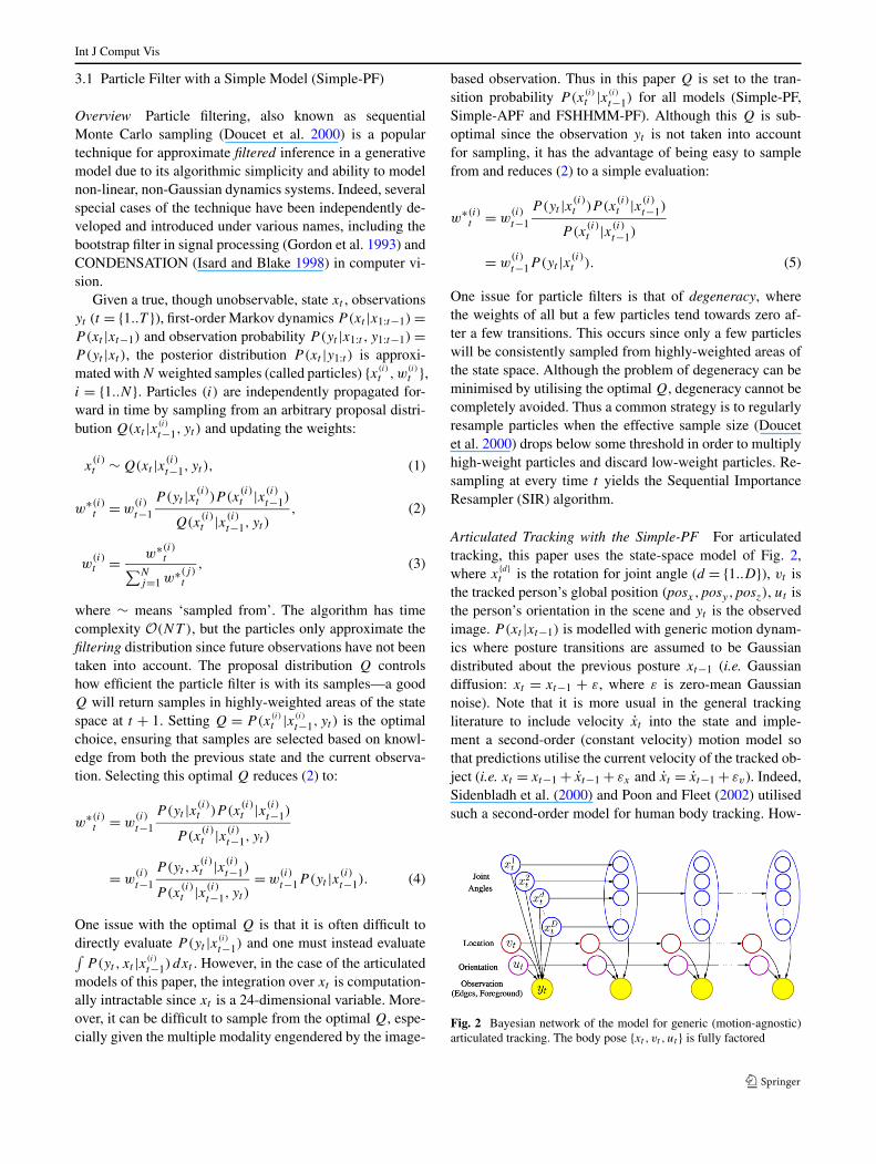
Articulated Tracking with the Simple-PF For articulatedtracking, this paper uses the state-space model of Fig. 2,where x

{d}t is the rotation for joint angle (d = {1..D}), vt is

the tracked person’s global position (posx,posy,posz), ut isthe person’s orientation in the scene and yt is the observedimage. P(xt |xt−1) is modelled with generic motion dynam-ics where posture transitions are assumed to be Gaussiandistributed about the previous posture xt−1 (i.e. Gaussiandiffusion: xt = xt−1 + ε, where ε is zero-mean Gaussiannoise). Note that it is more usual in the general trackingliterature to include velocity xt into the state and imple-ment a second-order (constant velocity) motion model sothat predictions utilise the current velocity of the tracked ob-ject (i.e. xt = xt−1 + xt−1 + εx and xt = xt−1 + εv). Indeed,Sidenbladh et al. (2000) and Poon and Fleet (2002) utilisedsuch a second-order model for human body tracking. How-

Fig. 2 Bayesian network of the model for generic (motion-agnostic)articulated tracking. The body pose {xt , vt , ut } is fully factored

Int J Comput Vis

ever, later work by Balan et al. (2005) showed that second-order models actually perform worse in human body track-ing than first-order (diffusion) approaches due to the highlynon-linear nature of human motion. Such issues could beovercome by particle-filtered inference on a non-linear, non-Gaussian model of human motion since the particle filter-ing framework is not restricted to linear Gaussian models.However, such a model (e.g. as implemented by this paperin Sect. 3.3) requires significantly more effort to constructthan the Simple-PF. Hence this paper employs first-orderGaussian diffusion transition dynamics for the Simple-PF.

The Simple-PF also assumes that xt fully factorises intoits component degrees of freedom (i.e. the covariance ofeach joint’s rotations is diagonal), with variances set basedon the maximum change in rotation over one frame. Thisgreatly simplifies the task of manually specifying rotationvariances and allows the model to generically represent anyhuman motion, at the cost of a weak motion model andhence poor proposal distribution Q(xt |xt−1). To offset thisweakness filtering is performed with 10,000 particles, a rel-atively large amount for a generative body tracker. Moresophisticated generic approaches could have been used tomake the model more efficient, such as dynamically adjust-ing the covariance (Sminchisescu and Triggs 2001). How-ever, this paper deals with articulated tracking in the pres-ence of occluding objects, and the simpler model makesfewer assumptions that may prove to be invalid during timesof occlusions and other problematic observations.

3.2 Annealed Particle Filter w/Simple Model(Simple-APF)

Overview The annealed particle filter (APF), first pro-posed by Deutscher and Reid (2005), is a variant of the SIRparticle filter where initial particles generated from a particlefilter prediction step at time t are iteratively perturbed andresampled based on an annealing schedule. The annealingcauses the system to gradually cluster particles into peaks of

the observation likelihood by weighting the likelihood:

P�(yt |xt ) = P(yt |xt )λ� , 0 < λ1 < · · · < λL, (6)

where P�(·) is the annealed likelihood at the �-th anneal-ing iteration (� = {1..L}). The monotonically increasing val-ues of the annealing powers λ� cause P�(·) to become morepeaked as the schedule progresses, thereby placing increas-ing emphasis on particles in more-likely parts of the ob-servation. At each iteration �, the particles are evaluatedwith (6), resampled to proliferate the best particles and thenperturbed via Gaussian diffusion to search the neighbour-hood around these best particles. The process is repeateduntil the annealing schedule is completed. In this way, theAPF gradually focuses its search in the peaks of the obser-vation likelihood at time t .

Articulated Tracking with the Simple-APF The Simple-APF uses the same generic motion model with indepen-dent (fully-factorised) joint rotations and Gaussian diffu-sion for posture transitions that the Simple-PF employs,(Fig. 2). Similarly, 10,000 particles are used for APF infer-ence but these are empirically split into 10 annealing lay-ers of 1,000 particles each. In comparison with the Simple-PF, the Simple-APF will typically produce particle sets thatare densely packed in the observation likelihood peaks andsparser elsewhere due to the iterative annealing.

3.3 Particle Filter with a Factored-StateHierarchical Hidden Markov Model (FSHHMM-PF)

Overview The FS-HHMM (Fig. 3) is a two-level hierarchy(Peursum et al. 2007) that addresses the problem of com-pactly representing the non-linear dynamics of articulatedhuman motion in a Bayesian setting. The model is parame-terised as follows:

Cmn � P(qt,n|qt−1,m), (7a)

A{d}nij � P(x

{d}t,j |x{d}

t−1,i , qt,n, e{d}t = 0), (7b)

Fig. 3 Bayesian network of theFS-HHMM for learning-basedarticulated tracking. Source:Peursum et al. (2007), © 2007IEEE

Int J Comput Vis

�{d}nj � P(x

{d}t,j |qt,n, e

{d}t = 1), (7c)

φm � P(q1,m), (7d)

ϕ{d}mi � P(x

{d}1,i |q1,m), (7e)

�{d}nmi � P(e

{d}t |x{d}

t−1,i , qt−1,m, qt,n), (7f)

{g} � P(v{g}t |v{g}

t−1), (7g)

ϒt � ωu|ut P (ut |ut−1) + ω

u|vt P (ut |vt−1, vt ), (7h)

where {x{1:D}t , v

{1:G}t , ut } represents the posture, position and

orientation of the person’s body and qt is the phase of themotion (described below). Omitted is the observation func-tion P(yt |x{1:D}

t , v{1:G}t , ut ), since it is a fixed heuristic that

evaluates the posture {x{1:D}t , v

{1:G}t , ut } against the observed

image, as described in Sect. 3.4. For more details on the FS-HHMM see Peursum et al. (2007).

The FS-HHMM models a single human action (e.g. walk-ing) by breaking it down into phases (sub-motions) that de-fine a set of valid possible body configurations (postures)and their transitions. The discrete nature of the HHMM al-lows for learning arbitrary non-linear motion, an importantfactor since human motion is not well-modelled with lin-ear dynamics (Balan et al. 2005). The phase qt facilitatesfactorising the body joint rotations—by assuming rotationsare conditionally independent given the phase, a particu-lar phase defines a transition regime for each rotation andcollectively these regimes define the coordinated motion ofthe limbs for the sub-motion represented by the phase. Notethat the FS-HHMM models body joint rotations with a dis-crete xt rather than the continuous xt of the Simple-PF andSimple-APF. As mentioned, this allows for learning arbi-trary non-linear motion transition distributions (Anij and�nj ), at the cost of some loss in accuracy due to discreti-sation.

Articulated Tracking with the FSHHMM-PF As with theSimple-PF and Simple-APF, the FSHHMM-PF utilises aparticle filter for approximate inference,with a proposal dis-tribution Q � P(xt |xt−1). This Q is learned from trainingdata of the motion being represented (e.g. walking) and sowill channel particle-filtered sampling down good areas ofthe predicted posture space (assuming that the person is per-forming the modelled motion). Hence only 1,000 particlesare needed to provide reliable body tracking, far fewer thanthe generic Simple-PF and Simple-APF models. For this pa-per, an FS-HHMM is trained with a single walking sequenceof four steps along a straight line. This training data is suf-ficient to model and track most walking motions (includingturns and pivoting).

3.4 Body Model and Observation Function

All three filtering models employ the same body model andobservation function. This paper focuses on human posetracking with generative Bayesian models where the obser-vation function is projection-based to improve robustnessto observation errors such as occlusions by scene objects(Peursum et al. 2007). A loose-fitting body model is used toavoid the need to manually tune it to the specific physiquesof the people being tracked.

Body Model This paper employs a 28-dimensional modelof the human body (Fig. 4), rooted at the pelvis and pa-rameterised by 24 joint rotations and four global variables(x, y, z, orientation—body pitch is modelled at the pelvisso that it can be learned by the FSHHMM-PF) as well asa fixed scale. Scale applies to the entire body model sincethe relative length of each limb is fixed. Each body part ismodelled with a cylinder whose sides are projected onto the2D image and then joined with lines to produce the card-board look for efficient projection (Sidenbladh et al. 2000).The model is fairly loose-fitting so that any tracker basedon it should generalise well to different people. Broad limitson joint rotations are enforced to constrain postures to thosethat are feasible for most human motions, but these limitsare not specific to any particular motion. No effort is madeto prevent body part intersection in 3D space.

Observation Likelihood Function This uses an observationfunction P(yt |xt ) based on projecting xt onto the imageyt and evaluating the difference between the two. Here, yt

is a tuple consisting of the edges and foreground images.Foreground is extracted using a mixture of Gaussians back-ground subtraction (Stauffer and Grimson 2000) and edgesare extracted with a thresholded Sobel detector, with the

Fig. 4 28D ‘cardboard’ body model. Source: Peursum et al. (2007),© 2007 IEEE

Int J Comput Vis

foreground used as a mask on the edges. A modified ver-sion of the cost function of Deutscher and Reid (2005) isemployed:

D = Dist(yt ,Proj(xt )

)(8)

which calculates the ‘distance’ between yt and the fore-ground/edges projections of xt (see Peursum 2006 for de-tails). For the particle-filtered models in this paper (i.e.Simple-PF and FSHHMM-PF), the observation probabilityP(yt |xt ) is then calculated via the exponential distributionand D:

P(yt |xt ) = λe−λD, (9)

where λ > 0 and D � 0. The value of λ controls how sharplythe distribution drops off with increasing values of D (i.e.increasing distance), hence a larger λ will more heavily pe-nalise slightly incorrect particles. This is important sincemost particles will return similar values for D due to thehigh dimensionality of the state space. For example, if twoparticles only differ significantly in their elbow angles, 95%(27 of 28D) of the body model is still much the same, plusthe forearm is not a large body part in the projection andmay even be occluded in some views.

For the APF, the observation probability is defined as fol-lows (according to Deutscher and Reid 2005):

f (yt |xt ) = (e−D

)λ, (10)

where the APF’s algorithm automatically sets λ, usuallysuch that λ � 1 so that slightly incorrect particles are heav-ily penalised. Notice that, unlike (9), this function is not aprobability density since it does not integrate to 1.0 unlessλ = 1. However, note also that since particles in this pa-per are weighted by P(yt |xt ) (see (5)) and then normalised,the proportionality constant multiplier λ in (9) is redundantsince it will be normalised away. With this insight in mind, itis possible to see that (9) and (10) are effectively equivalent:

P(yt |xt ) = λe−λD

= λ(e−D

)λ

∝ (e−D

)λ

∝ f (yt |xt ). (11)

In other words, applying the annealing factor λ of the APFas a power is merely another way of writing the general formof the exponential distribution (disregarding the proportion-ality constant, which is redundant in the particle filter due tonormalisation). Thus a suitable λ � 1 could be chosen forthe Simple-PF to define its observation probability and sim-ilar performance to the Simple-APF should result—this isprecisely what is found in Sect. 6.1. Due to this equivalence,

this paper will henceforth refer to λ as the annealing fac-tor (rather than a more cumbersome term like ‘exponentialcoefficient’).

However, there is still an important difference betweenthe particle filter and the APF in that the APF selects thevalue of λ dynamically for each annealing layer. This meansthat the APF is continually altering its definition of P(yt |xt )

between annealing layers and time instants—one can arguethat this means the Simple-APF is not strictly a Bayesianmodel. Indeed, the authors themselves make note of thisin (Deutscher et al. 2000). The Simple-PF and FSHHMM-PF do not suffer from this problem since λ in (9) is fixedacross all time instants, with values chosen empirically asλ = 8 and λ = 10 respectively (the Simple-PF’s weak mo-tion model necessitates more aggressive ‘annealing’).

Although the observation probability is heuristic in that itis constructed around the heuristic function D, most genera-tive human body trackers are forced to utilise such heuristicsdue to the difficulty of constructing and learning an alge-braic function that will produce a usable measure of similar-ity between the state and observation in arbitrary scenes. Theconsequence of using heuristics is that it creates an obser-vation probability that cannot be trained and so will returnerroneous results during unforeseen circumstances such aspartial occlusions. Hence what this paper describes as ‘ob-servation errors’ are in fact failures of D to properly accountfor the observation.

4 Smoothed Articulated Tracking

4.1 Issues of Existing Smoothing Techniques

As has been discussed, smoothed inference is rare in ar-ticulated tracking. Part of the reason for this is that thehigh dimensionality of the posture space means that ap-proximate filtering is already a computationally expensivetask, and smoothing only adds to this cost. However, overthe past decade there has been increasing use in trackingand signal processing of efficient approximate smoothed-inference techniques such as variational approximations,Markov Chain Monte Carlo (MCMC) methods and particlesmoothing.

A variational approach to smoothed inference has greatpotential for articulated tracking since it has been shownto scale well to high dimensionality (Ghahramani and Jor-dan 1997). MCMC methods such as Gibbs sampling (An-drieu et al. 2003) are also worthwhile exploring given theirflexibility and typically polynomial (though difficult-to-measure) convergence. Finally, the forward-filter backward-smoother (Doucet et al. 2000) or two-filter smoother (Klaaset al. 2006) for particle filters would be obvious smoothingchoices for existing particle-filtered methods. However, all

Int J Comput Vis

of these approaches face obstacles when applied to articu-lated tracking in a generative model:

– Variational methods require the ability to take expecta-tions and derivatives of the joint probability parameters.However, the observation likelihood function in a gener-ative tracker is often implemented as a complex heuris-tic function. Such functions are difficult to express alge-braically (precluding analytical solutions) and are compu-tationally expensive to evaluate (making numerical meth-ods such as gradient descent and MCMC integration im-practical).

– MCMC/Gibbs sampling also face difficulties with thehigh computational cost of the heuristic observation func-tion. Efforts to obtain a faster observation function (e.g.Caillette et al. 2005) rely on extracting a 3D visual hullfor the observation, but this requires multiple views andis sensitive to observation errors (e.g. occlusions by sceneobjects), thus robustness will suffer accordingly.

– Particle smoothing algorithms do not require evaluationsof the observation function but are limited to adjustingparticle weights and so will not explore new parts of theposture space during smoothing. In addition, these algo-rithms have O(N2T ) complexity where N is the numberof particles, which may be computationally impracticalsince N is usually quite large.

Most of the issues centre around the computational costof executing the various smoothing algorithms. This pa-per proposes to facilitate efficient execution of variationaland Gibbs methods by approximating the computationally-costly observation function with a mixture of Gaussians de-rived from a pre-processing particle filter. Particle smooth-ing is also implemented and shown to have a reasonablecomputational cost with respect to filtering for N � 10,000due to the high overheads that the projection-based obser-vation likelihood adds to filtering. Note that this paper con-siders a smoothing algorithm to be “computationally fea-sible” if its runtime is comparable to, or less than, that ofthe pre-processing particle filter run on the same sequence.Complexity analysis (O-notation) is not suitable here sinceit does not indicate constant overheads and there is no wayof comparing algorithms whose complexity terms differ.

4.2 Particle Smoothing

There are several methods that have been proposed to pro-vide smoothed inference from a forward pass by a particlefilter: the forwards-backwards smoother (FBS; Doucet et al.2000), smoothed distribution sampling, (SS; Doucet et al.2002; Godsill et al. 2004), maximum a-posteriori smoother(MAP; Doucet et al. 2002; Klaas et al. 2006) and two-filtersmoother (TFS; Klaas et al. 2006). While their details vary,all of these smoothing algorithms are essentially methods to

re-weight the particles of the initial filtering pass to take intoaccount the future data. The particles themselves are not ad-justed towards better areas of the state space. Moreover, allare O(N2T ) complexity, although Klaas et al. (2006) de-scribes an approximate technique using KD-trees that canreduce this to O((N logN)T ).

The FBS calculates new weights for the particles at eachtime t by considering the level of ‘support’ that each parti-cle has in the future, where support is the mass of particlesat time t + 1 that a particle x

(i)

t could (hypothetically) tran-sition to, weighted by the probability of those transitions.This iterates from T − 1 . . .1, carrying the smoothing back-wards until all weights are smoothed. The SS approach issubstantively similar to FBS, differing mainly in that theFBS re-weights the particles to estimate the smoothed dis-tribution whereas SS samples particles trajectories from thissmoothed distribution. Thus SS can be loosely viewed as aresampled version of FBS, consequently losing some of thesmoothed distribution’s information. The MAP smootheralso resamples, but differs from SS in that it computes aViterbi-like state path through the particle trellis and sam-ples only the single most likely particle trajectory (in a MAPsense), and so discards even more of the distribution than SS.

In contrast to the other methods, the TFS approach in-volves a second, independent, particle filter that is run inreverse (from T to 1). The smoothed particle weights arecalculated based on the mutual support between the two fil-ters’ particle sets, much like the FBS weight update. Unlikethe other particle smoothing methods, the reverse run allowsthe TFS to explore parts of the state space not represented bythe forward filter. However, the trajectories of the particlesin the two filters must overlap somewhat in order for thereto be reasonable support between particles in the two filters.Given that the reverse filter evolves independently of the for-ward filter, this overlap can be difficult to guarantee in high-dimensional state spaces. In 28D human posture tracking itis possible that the reverse filter explores a local maxima ofthe state space that is entirely isolated from the forward filterat a given time t . In such a case, the mutual support betweenthe two particle sets may not be very meaningful. Finally, thereverse filter is itself a significant processing overhead forgenerative trackers where the observation function is slowto evaluate. Due to the reduced information of SS and MAPand the potential issues of TFS, this paper employs FBS.

4.3 Mixture Approximation of P(yt |xt )

4.3.1 Motivation and Overview

The fact that particle smoothers do not shift the position ofthe filtering particles given the future evidence from smooth-ing is their main drawback. Ideally, smoothing would ex-plore new areas of the state space that both past and fu-ture evidence indicates is promising (the TFS reverse filter

Int J Comput Vis

ignores the past and so is no better than the forward filter).This is particularly important for posture tracking in realisticscenes, where posture failures caused by (say) an occludingchair tend to ‘stick’ until the occlusion ceases or the errorbecomes large enough to force the tracker to correct itself(Peursum et al. 2007). For particle smoothers, the gap be-tween the failure and the correction is a void that cannot befilled since no particles exist in this space. This motivatesthe search for other smoothed inference algorithms that arenot so restrictive.

Unfortunately, as described in Sect. 4.1, existing approxi-mate inference techniques cannot be applied directly to gen-erative pose tracking, mostly due to the computational costof the observation function P(yt |xt ). This paper resolvesthis by approximating P(yt |xt ) with a more manageablefunction P (yt |xt ). Since the observation function employedin this paper is based on heuristic edge and foreground com-parisons between the projected body model and the obser-vation, approximating the function in general (i.e. for anyobservation-model pairing) is not an easy task. However, adiscrete approximation of P(yt |xt ) is available from particlefiltering—to evaluate a particle i, P(yt |x(i)

t ) must be calcu-lated. In effect, each particle can be thought of as samplingfrom P(yt |xt ) with a weight equal to the function’s prob-ability at x

(i)

t . P(yt |xt ) could then be approximated witha Gaussian mixture P (yt |x(i)

t ) that is learned from theseweighted samples:

P(yt |xt ) ≈ P (yt |xt ) =K∑

k=1

ηk N (xt |μk, k), (12)

where N is the Gaussian distribution and ηk , μk and k arethe weight, mean and covariance for component k. In thispaper, the covariance is held constant for all mixture com-ponents, hence the mixture is quite similar to kernel densityestimation (KDE, also known as Parzen window density es-timation). The main difference from KDE is that the mixtureadjusts the weights for each component via learning. This iscrucial since otherwise the approximation will not faithfullyreflect the true observation probability distribution P(yt |xt ).A lesser difference is that mixture learning also shifts thecomponent means about, although in practice the shifts aresmall and if one fixes the means (as in KDE) a very similarapproximation is produced.

To illustrate the need for adjusting the component/kernelweights, consider the case of kernel density estimation withGaussian kernels, where each particle is the kernel fora component (i.e. μk = x

(i)

t , K = N ). If each kernel isweighted by the observation probability of the particle thatgenerated it, the probability of any given xt = xt is then:

P (yt |xt ) =N∑

i=1

ρ(i)N (xt |x(i)t , ), (13)

Fig. 5 (Color online) Example mixture approximation generated fromparticle filter samples. Solid green curve is the true function P (yt |xt );vertical blue bars indicate particles; dashed red curve is the mixtureapproximation P (yt |xt ) produced from the Gaussian components (thindashed orange)

where ρ(i) = P(yt |x(i)t ). The problem with this definition is

that the weights of closely-spaced components (e.g. com-ponents less than one standard deviation apart) will addup, causing P (yt |x(i)

t ) � P(yt |x(i)t ) at these closely-packed

points and thus misrepresenting P(yt |xt ). Hence it is neces-sary to adjust the weights (and optionally shift the means)via Expectation-Maximisation (EM) in order to faithfullyreplicate the values of P(yt |x(i)

t ) with the mixture.In comparison to the discrete particles, the continuous

nature of the Gaussian mixture should be a better repre-sentation of the similarly-continuous P(yt |xt ), as depictedin Fig. 5. In particular, the mixture will partially ‘fill in’the voids between the discrete particles, providing a reason-able representation of the observation function’s behaviourin the vicinity of the particles. The idea is that the mixturewill facilitate a range of inference techniques and providethem with some flexibility in exploring the state space whilstremaining acceptably accurate to the true P(yt |xt ). Subse-quent inference is then effectively a smoothing of the origi-nal particle filter used to generate the mixture.

4.3.2 Learning the Gaussian Mixture

Learning a Gaussian mixture model (GMM) via EM is awell-known procedure. Given data xi , i = {1..N} and Gaus-sians with K components whose means, covariances andweights are {μk, k, ηk}, k = {1..K}, the EM update equa-tions for estimating a GMM are:

τi,k = ηk N (xi |μk, k)∑K

j=1 ηj N (xi |μj , j ), (14)

ηk = 1

N

N∑

i=1

τi,k, (15)

μk =∑N

i=1 τi,kxi∑N

i=1 τi,k

, (16)

Int J Comput Vis

k =∑N

i=1 τi,k(xi − μk)(xi − μk)T

∑Ni=1 τi,k

, (17)

where it is preferred that K�N for the sake of efficiency.For the particle-filtered samples, each xi � x

(i)

t has an as-sociated weight ρi = P(yt |x(i)

t ). This can be incorporatedinto the EM equations by reinterpreting the weights as rep-resenting the relative number of samples at each location xi .For example, the update for ηk becomes η′

k = 1Z

∑Ni=1(ρiτi,k),

as if there were ρi -worth of data points at xi (where Z =N × ∑

j ρj ). Since τi,k is the weight for the assignment ofxi to Gaussian k and ρi is the weight of each xi , one willfind that τi,k always occurs together with ρi . Hence it is con-venient to define τ ′

i,k = ρiτi,k . The update equations for the

GMM approximation P (yt |xt ) at a given t thus become:

τ ′i,k = ρiτi,k � ρi

η′k N (xi |μk, k)

∑Kj=1 η′

j N (xi |μj , j ), (18)

η′k = 1

N∑

j ρj

N∑

i=1

τ ′i,k, (19)

μ′k =

∑Ni=1 τ ′

i,kxi∑N

i=1 τ ′i,k

, (20)

′k =

∑Ni=1 τ ′

i,k(xi − μk)(xi − μk)T

∑Ni=1 τ ′

i,k

. (21)

The usual practical issues arise in the approximation, in-cluding deciding how many components K to use, the ini-tial value of each component’s parameters and whether toplace any constraints on the EM updates. Due to the highdimensionality of P(yt |xt ) (28D), this paper is fairly con-servative in its choices to avoid causing P (yt |xt ) to becomeunrepresentative of the true P(yt |xt ). There is however atradeoff between speed and faithfully representing P(yt |xt ).Hence Gaussian modes are chosen based on the distributionof samples (by weight), selecting all samples that are above-average (i.e. ρi � 1

N

∑j ρj ) and using the corresponding

value of x(i)

t as the initial mean for each mode. The assump-tion is that below-average particles are in uninteresting ar-eas of P(yt |xt ) and so can be safely ignored as seeds formixture components. K is roughly the same as the filter’seffective sample size at each time t , which in this paperis between 0.05N and 0.2N . As with particle resampling,the approach retains more mixture components during timesof problematic observations such as when occlusions oc-cur. These cause the effective sample size to increase (i.e.the distribution becomes more uniform) since all particlesare somewhat in error according to P(yt |xt ) due to the oc-clusion. Conversely, fewer samples are retained with cleanobservations. This behaviour is desirable—during an occlu-sion, particles that are more probable according to P(yt |xt )

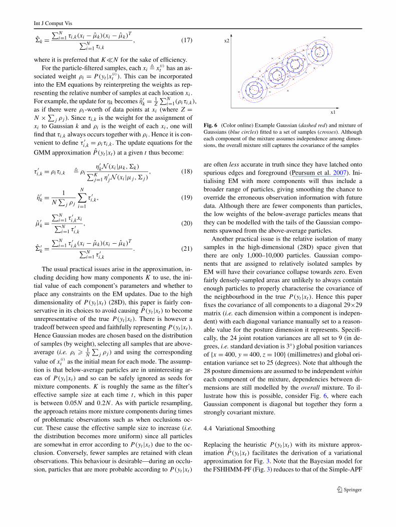
Fig. 6 (Color online) Example Gaussian (dashed red) and mixture ofGaussians (blue circles) fitted to a set of samples (crosses). Althougheach component of the mixture assumes independence among dimen-sions, the overall mixture still captures the covariance of the samples

are often less accurate in truth since they have latched ontospurious edges and foreground (Peursum et al. 2007). Ini-tialising EM with more components will thus include abroader range of particles, giving smoothing the chance tooverride the erroneous observation information with futuredata. Although there are fewer components than particles,the low weights of the below-average particles means thatthey can be modelled with the tails of the Gaussian compo-nents spawned from the above-average particles.

Another practical issue is the relative isolation of manysamples in the high-dimensional (28D) space given thatthere are only 1,000–10,000 particles. Gaussian compo-nents that are assigned to relatively isolated samples byEM will have their covariance collapse towards zero. Evenfairly densely-sampled areas are unlikely to always containenough particles to properly characterise the covariance ofthe neighbourhood in the true P(yt |xt ). Hence this paperfixes the covariance of all components to a diagonal 29×29matrix (i.e. each dimension within a component is indepen-dent) with each diagonal variance manually set to a reason-able value for the posture dimension it represents. Specifi-cally, the 24 joint rotation variances are all set to 9 (in de-grees, i.e. standard deviation is 3◦) global position variancesof {x = 400, y = 400, z = 100} (millimetres) and global ori-entation variance set to 25 (degrees). Note that although the28 posture dimensions are assumed to be independent withineach component of the mixture, dependencies between di-mensions are still modelled by the overall mixture. To il-lustrate how this is possible, consider Fig. 6, where eachGaussian component is diagonal but together they form astrongly covariant mixture.

4.4 Variational Smoothing

Replacing the heuristic P(yt |xt ) with its mixture approx-imation P (yt |xt ) facilitates the derivation of a variationalapproximation for Fig. 3. Note that the Bayesian model forthe FSHHMM-PF (Fig. 3) reduces to that of the Simple-APF

Int J Comput Vis

and Simple-PF (Fig. 2) when there is only one phase qt . Thedifference between the two is that the Simple-PF/Simple-APF posture is continuous and has Gaussian diffusion tran-sitions, whereas the FSHHMM-PF is discrete to allow formodelling arbitrary non-linear/non-Gaussian motion in itstransition distributions. Therefore, rather than derive twosets of variational update equations for what is essen-tially the same model, we derive the approximation forthe discrete FSHHMM-PF and reuse this for the Simple-PF/Simple-APF by quantising their filtered postures andhand-crafting a discrete generic transition model that repli-cates their Gaussian diffusion dynamics. This entails someloss of accuracy on the part of the continuous Simple-PF andSimple-APF, but the quantisation error is small when com-pared to errors caused by tracking failures due to occlusionsand poor observations (Peursum et al. 2007). Moreover, themanual ground-truth obtained with virtual markers is onlyaccurate to within about ±50 mm. The remainder of thissection describes the changes made to the FSHHMM-PFmodel of Fig. 3 for the purposes of variational and Gibbsapproximation.

4.4.1 Graphical Model with the Mixture

Figure 7a depicts the adjusted FS-HHMM used for varia-tional approximation of posture, where P(yt |xt ) has beensubstituted with the mixture approximation P (yt |xt ). Themodel parameters differ slightly from that of the original FS-HHMM in Fig. 3. Equations (7a)–(7e) remain unchanged.Additional parameters are:

η(k)t � P(s

(k)t ), (22a)

P(y{d}x,t |x{d}

t ) =K∑

k=1

η(k)t N (x

{d}t |y{d}(k)

x,t ,R{d}yx

), (22b)

P(y{g}v,t |v{g}

t ) =K∑

k=1

η(k)t N (v

{g}t |y{g}(k)

v,t ,R{g}yv

), (22c)

P(yu,t |ut ) =K∑

k=1

η(k)t N (ut |y(k)

u,t ,Ryu) (22d)

and (7g) and (7h) are changed to:

t � P(v{g}t ) = N (vt |μ{g}

v,t , {g}v,t ), (22e)

ϒt � P(ut ) = N (ut |μu,t , u,t ), (22f)

where st in (22a) is the mixture component ‘selector’ ex-pressed as a Boolean vector s

(k)

t k = {1..K} and η(k)

t isthe mixture weights (k is indexed as a superscript to rein-force the fact that mixture components (k) arise from parti-cles (i)). The means for the 28 dimensions of each compo-nent k in the observation mixture are split across body jointangles x

{d}t , global body position v

{g}t , g ∈ {posx,posy,posz}

(the g factors are not explicitly shown in the figure) andglobal body orientation ut . Observation mixture means arethus defined as y

{d}(k)

x,t , y{g}(k)

v,t and y{g}(k)

u,t respectively, with as-sociated empirically-specified variances R

{d}yx

, R{g}yv

and Ryu .Note the peculiarity that the observations yx,t are in fact themeans of the Gaussian mixture and xt is the data variable,rather than vice-versa as P(yt |xt ) would imply. This isn’ta problem since Gaussians are symmetric about their mean,hence viewing either variable as the mean is equivalent.

{μ{g}v,t ,

{g}v,t } and {μu,t , u,t } are the means and variances

for the priors on vt and ut . Note that the dynamics de-pendencies P(vt |vt−1) and P(ut |ut−1) have been dropped;this has been facilitated by the mixture’s properties. Specif-ically, the mixture has low variance for the dimensions rep-resenting the person’s global 3D position and orientation{y{g}

v,t , yu,t }. This is due to the fact that these dimensions lie atthe very root of the body model’s kinematic tree (see Fig. 4)and so do not accumulate the uncertainties of nodes higherup in the tree. In other words, P(yt |vt , ut ) is non-zero onlyin a small area and so the dynamics dependencies are largelyredundant. In fact, the assumption of the linear dynamicsmodel for P(vt |vt−1) is actually detrimental since people donot move in a strictly linear fashion, but the dynamics willerroneously bias a variational approximation towards suchlinear motion. Instead, P(vt ) and P(ut ) are characterisedby fitting a Gaussian to the particles of the pre-processingfilter:

μ{g}v,t =

∑

i

w(i)t v

{g}(i)t , (23a)

{g}v,t =

∑

i

(w

(i)t v

{g}(i)t

)2 − (μ

{g}v,t

)2, (23b)

μu,t =∑

i

w(i)t u

(i)t , (23c)

u,t =∑

i

(w

(i)t u

(i)t

)2 − (μu,t

)2. (23d)

4.4.2 Variational Equations

Variational approximation proceeds by obtaining a lowerbound on the log-likelihood of the true posterior P =P(x1:T |y1:T ) using a more tractable distribution Q(x1:T ).This lower bound is achieved by varying Q to minimise theKullback-Liebler (KL) divergence between P and Q, whereKL is defined as:

KL(Q‖P ) =∫

Q(x1:T ) log

( Q(x1:T )

P (x1:T |y1:T )

)

dx1:T

=∫

Q(x1:T ) log Q(x1:T ) dx1:T

−∫

Q(x1:T ) log P (x1:T |y1:T ) dx1:T

= EQ〈log Q〉 − EQ〈log P 〉, (24)

Int J Comput Vis

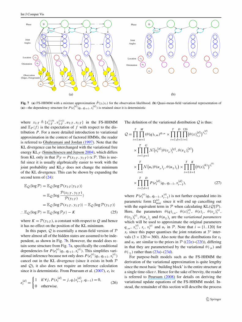
Fig. 7 (a) FS-HHMM with a mixture approximation P (yt |xt ) for the observation likelihood. (b) Quasi-mean-field variational representation of(a)—the dependency structure for P (e

{d}t |qt , qt+1, x

{d}t ) is retained since it is deterministic

where x1:T � {x{1:D}1:T , v

{1:G}1:T , u1:T , s1:T } in the FS-HHMM

and EP 〈f 〉 is the expectation of f with respect to the dis-tribution P . For a more detailed introduction to variationalapproximation in the context of factored HMMs, the readeris referred to Ghahramani and Jordan (1997). Note that theKL divergence can be interchanged with the variational freeenergy KLF (Sminchisescu and Jepson 2004), which differsfrom KL only in that PF = P(x1:T , y1:T ) ∝ P . This is use-ful since it is usually algebraically easier to work with thejoint probability and KLF does not change the minimumof the KL divergence. This can be shown by expanding thesecond term of (24):

EQ〈log P 〉 = EQ〈log P (x1:T |y1:T )〉

= EQ〈logP (x1:T , y1:T )

P (y1:T )〉

= EQ〈log P (x1:T , y1:T )〉 − EQ〈log P (y1:T )〉∴ EQ〈log P 〉 = EQ〈log P F 〉 − K (25)

where K = P (y1:T ), a constant with respect to Q and henceit has no effect on the position of the KL minimum.

In this paper, Q is essentially a mean-field version of Pwhere almost all of the hidden states are assumed to be inde-pendent, as shown in Fig. 7b. However, the model does re-tain some structure from Fig. 7a, specifically the conditionaldependencies for P(e

{d}t |qt , qt+1, x

{d}t ). This simplifies vari-

ational inference because not only does P(e{d}t |qt , qt+1, x

{d}t )

cancel out in the KL divergence (since it exists in both Pand Q), it also does not require an inference calculationsince it is deterministic. From Peursum et al. (2007), et is:

e{d}t =

{1 if ∀j,P (x

{d}t = j, qt |x{d}

t−1, qt−1) = 0,

0 otherwise.(26)

The definition of the variational distribution Q is thus:

Q =T∏

t=1

M∏

m=1

(θ(q)t,m)qt,m ×T∏

t=1

D∏

d=1

120∏

i=1

(θ(x)

{d}t,i

)x{d}t,i

×T∏

t=1

G∏

g=1

N(v

{g}t |θ(vμ){g}

t, θ(v )

{g}t

)

×T∏

t=1

N(ut |θ(uμ)

t, θ(u )t

) ×T∏

t=1

K∏

k=1

(θ(s)

(k)t

)s(k)t

×T∏

t=2

D∏

d=1

P(e{d}t |qt , qt−1, x

{d}t−1), (27)

where P(e{d}t |qt , qt−1, x

{d}t−1) is not further expanded into its

parametric form �{d}mni since it will end up cancelling out

with the equivalent term in P when calculating KL(Q‖P ).Here, the parameters θ(q)t,m , θ(x)

{d}t,i , θ(s)t , θ(vμ)

{g}t ,

θ(v ){d}t , θ(uμ)

tand θ(u )t are the variational parameters

which will be used to approximate the original parametersqt,m , x

{d}t,i , st , v

{g}t and ut in P . Note that i = {1..120} for

xt since this paper quantises the joint rotations at 3◦ inter-vals (3 × 120 = 360). Also note that the distributions for vt

and ut are similar to the priors in P ((22e)–(22f)), differingin that they are parameterised by the variational θ(·μ) andθ(· ) rather than (23a)–(23d).

For purpose-built models such as the FS-HHMM thederivation of the variational approximation is quite lengthysince the most basic ‘building block’ is the entire structure ata single time-slice t . Hence for the sake of brevity, the readeris referred to Peursum (2008) for details on deriving thevariational update equations of the FS-HHMM model. In-stead, the remainder of this section will describe the process

Int J Comput Vis

of utilising the update equations found in (Peursum 2008).Briefly, to derive the update equations one must plug (27)and the equivalent equation for the joint probability of Pinto the KL divergence (24), then take derivatives with re-spect to the various θ(·) parameters and solve for zero. Thisleads to a set of fixed-point update equations. Note that todo this, the dynamic Bayesian networks of Fig. 7 are be-ing implicitly ‘unrolled’ across time to match the length ofthe observed sequence y1:T , hence the list of θ(·) variablesis also fixed (i.e. the variational updates are occurring on afixed network).

These θ(·) are then optimised by iteratively evaluatingall the fixed-point equations for each θ(·) one round at atime. Specifically, a single iteration round involves calculat-ing the new value of each θ(·) in turn using the latest ver-sion of all the other θ(·)’s (i.e. use the new values of θ(·)’sthat were updated earlier in the current iteration round). Theorder of updating the θ(·) variables is in terms of movingalong the Bayesian network from top-to-bottom (qt beforext ) and left-to-right (t = 1 before t = 2, etc.), although con-vergence should occur regardless of the chosen ordering. It-erating these update rounds will then converge to a locallyoptimal solution, where convergence is monitored by cal-culating the KL divergence after each update iteration, andcomparing this to the previous iteration’s KL divergence.

4.5 Gibbs Smoothing

As with the variational approximation, Gibbs inference (An-drieu et al. 2003; Ghahramani and Jordan 1997) uses themodel described in Sect. 4.4.1, with the Bayesian networkof Fig. 7a. Gibbs sampling is one of the simplest MarkovChain Monte Carlo methods, and proceeds by implicitly un-rolling the dynamic Bayesian network to a fixed networkof length T to match the observed sequence y1:T . Hiddenstates are then set to an initial value before repeatedly sam-pling new values for each state given its Markov blanketuntil N samples of the full joint distribution are drawn.Sampling occurs in rounds, where during round p a sam-ple is drawn for each hidden state given the current valueof the other states (whose value may have been updatedearlier in round p, depending on the order of processing).Again, the order in which the states are processed is fromtop-to-bottom and left-to-right along the Bayesian network.Once all states have been sampled the process is repeated forround p+1, continuing until p = N . The full set of sampledvalues over all rounds N then provides the sufficient statis-tics for the Gibbs estimate of each state—in the case of a dis-crete distribution this is the histogram of the samples and fora Gaussian it is the sample mean and covariance. See Peur-sum (2008) for details on the Gibbs sampling distributionsnecessary for Fig. 7a. Intuitively, Gibbs sampling works bydrawing a new sample that is ‘consistent’ with the current

values of states that can influence it (i.e. its Markov blan-ket). This consistency is then propagated along the networkone link at a time, resulting in states concentrating their sam-pling in areas of the state space that ‘make sense’ given thestate’s location in the unrolled Bayesian network. Eventuallythis leads to the samples effectively being drawn from thetrue posterior P(xt |y1:T ). Since the initial values may not bevery consistent with each other, the Markov sampling chainusually requires time (called burn-in) to converge to sam-pling from P(x1:T |y1:T ). Thus the first 5%–10% of samplesare typically excluded from the final Gibbs estimate. Thenumber of burn-in samples needed to achieve convergencedepends on the initial state values and the distributions beingsampled from, and is difficult to estimate in advance.

In this paper, the number of Gibbs samples is set to 2,000for the 1,000-particle FSHHMM-PF. Empirical tests showedthat values larger than 2,000 do not significantly improvethe Gibbs estimate, indicating that convergence has beenreached. For the Simple-PF/Simple-APF (10,000 particles),5,000 Gibbs samples are used. Although one would expectthat the 10× difference in filtering particles would suggestthe use of 20,000 Gibbs samples, the lower value of 5,000 ischosen so as to keep the computational runtime of Simple-PF/Simple-APF Gibbs smoothing in the same ballpark asthe computational time of Simple-PF/Simple-APF filtering.Burn-in time for all filters is set to the first 5% of Gibbssamples. See Sect. 5.2 for details on initialisation.

5 Experimental Setup

The filtering and smoothing algorithms described in this pa-per were evaluated against twelve video sequences—sevenHUMANEVA-I videos, two HUMANEVA-II sequences (Si-gal and Black 2006) and three CLUTTER videos capturedin scenes containing occluding tables and chairs. Each se-quence is processed with 12 algorithms (Table 1) to produce144 tracking results in total.

5.1 Test Scenes and Ground-Truth

Datasets Twelve video sequences of walking are usedfor test data, seven from the HUMANEVA-I dataset, twofrom the HUMANEVA-II dataset and three from CLUT-TER. The HUMANEVA sequences (Fig. 8) consists of severalvideos captured in tandem with marker-based motion cap-ture, hence actors are restricted to moving on a 3 m × 3 m

Table 1 Filtering and smoothing combinations (12 in total) employedfor tracking in each video

Int J Comput Vis

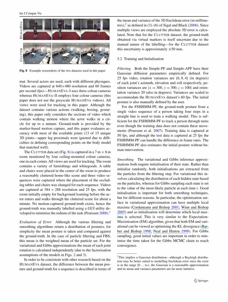
Fig. 8 Example screenshots of the two datasets used in this paper

mat. Several actors are used, each with different physiques.Videos are captured at 640×480 resolution and 60 framesper second (fps)—HUMANEVA-I uses three colour cameraswhereas HUMANEVA-II employs four colour cameras (thispaper does not use the greyscale HUMANEVA videos). Allviews were used for tracking in this paper. Although thedataset contains various actions (walking, boxing, gestur-ing), this paper only considers the sections of video whichcontain walking motion where the actor walks in a cir-cle for up to a minute. Ground-truth is provided by themarker-based motion capture, and this paper evaluates ac-curacy with most of the available joints (13 of 15 unique3D joints—upper leg proximals were ignored due to diffi-culties in defining corresponding points on the body modelthat matched well).

The CLUTTER data set (Fig. 8) is captured in a 7 m × 6 mroom monitored by four ceiling-mounted colour cameras,one in each corner. All views are used for tracking. The roomcontains a variety of furnishings and whitegoods. A tableand chairs were placed in the center of the room to producea reasonably cluttered home-like scene and three video se-quences were captured where the placement of the occlud-ing tables and chairs was changed for each sequence. Videosare captured at 384 × 288 resolution and 25 fps, with theroom initially empty for background learning before the ac-tor enters and walks through the cluttered scene for about aminute. No motion-captured ground-truth exists, hence theground-truth was manually labelled using a GUI utility de-veloped to minimise the tedium of the task (Peursum 2008).1

Evaluation of Error Although the various filtering andsmoothing algorithms return a distribution of postures, forsimplicity the mean posture is taken and compared againstthe ground-truth. In the case of particle filtering and FBS,this mean is the weighted mean of the particle set. For thevariational and Gibbs approximations the mean of each jointrotation is calculated independently (due to the factorisationassumptions of the models in Figs. 2 and 3).

In order to be consistent with other research based on theHUMANEVA dataset, the difference between the mean pos-ture and ground-truth for a sequence is described in terms of

the mean and variance of the 3D Euclidean error (in millime-tres),2 as defined in (3)–(6) of Sigal and Black (2006). Sincemultiple views are employed the absolute 3D error is calcu-lated. Note that for the CLUTTER dataset, the ground-truthobtained via virtual markers is itself uncertain due to themanual nature of the labelling—for the CLUTTER datasetthis uncertainty is approximately ±50 mm.

5.2 Training and Initialisation

Filtering Both the Simple-PF and Simple-APF have theirGaussian diffusion parameters empirically defined. For25 fps video, rotation variances are {6,8,4} (in degrees)of each joint’s azimuth, elevation and roll respectively, po-sition variances are {x = 300, y = 300, z = 100} and orien-tation variance 20 (also in degrees). Variances are scaled toaccommodate the HUMANEVA dataset’s 60 fps. The initialposture is also manually defined by the user.

For the FSHHMM-PF, the ground-truth posture from asingle video sequence of a person taking four steps in astraight line is used to train a walking model. This is suf-ficient for the FSHHMM-PF to track a person through turnseven though the training data does not contain these move-ments (Peursum et al. 2007). Training data is captured at50 fps, and although the test data is captured at 25 fps theFSHHMM-PF can handle the difference in frame rates. TheFSHHMM-PF also estimates the initial posture without hu-man intervention.

Smoothing The variational and Gibbs inference approxi-mations both require initialisation of their state. Rather thaninitialise randomly, both initialisations are extracted fromthe particles from the filtering step. For variational this in-volves calculating the distribution of each hidden state basedon the particles, whereas for Gibbs sampling each state is setto the value of the most-likely particle at each time t . Goodinitialisation is important for both smoothing techniques,but for different reasons. In particular, the optimisation sur-face in variational approximation can have multiple localmaxima (Corduneanu and Bishop 2001; Winn and Bishop2005) and so initialisation will determine which local max-ima is selected. This is very similar to the Expectation-Maximisation (EM) algorithm, given that both EM and vari-ational can be viewed as optimising the KL divergence (Bar-ber and Bishop 1998; Neal and Hinton 1998). For Gibbssampling, good initial values are important in order to min-imise the time taken for the Gibbs MCMC chain to reachconvergence.

2This implies a Gaussian distribution—although a Rayleigh distribu-tion may be better suited to modelling Euclidean error since the erroris in the range [0 . . .∞), the Gaussian is a reasonable approximationand its mean and variance parameters are far more intuitive.

Int J Comput Vis

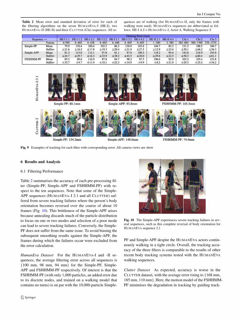
Table 2 Mean error and standard deviation of error for each ofthe filtering algorithms on the seven HUMANEVA-I (HE-I), twoHUMANEVA-II (HE-II) and three CLUTTER (Clu) sequences. All se-

quences are of walking (for HUMANEVA-II, only the frames withwalking were used). HUMANEVA sequences are abbreviated as fol-lows: HE-I A.S = HUMANEVA-I, Actor A, Walking Sequence S

Fig. 9 Examples of tracking for each filter with corresponding error. All camera views are show

6 Results and Analysis

6.1 Filtering Performance

Table 2 summarises the accuracy of each pre-processing fil-ter (Simple-PF, Simple-APF and FSHHMM-PF) with re-spect to the ten sequences. Note that some of the Simple-APF sequences (HUMANEVA-I 2.1 and all CLUTTER) suf-fered from severe tracking failures where the person’s bodyorientation becomes reversed over the course of about 10frames (Fig. 10). This brittleness of the Simple-APF arisesbecause annealing discards much of the particle distributionto focus on one or two modes and selection of a poor modecan lead to severe tracking failures. Conversely, the Simple-PF does not suffer from the same issue. To avoid biasing thesubsequent smoothing results against the Simple-APF, theframes during which the failures occur were excluded fromthe error calculation.

HumanEva Dataset For the HUMANEVA-I and -II se-quences, the average filtering error across all sequences is{100 mm, 98 mm, 94 mm} for the Simple-PF, Simple-APF and FSHHMM-PF respectively. Of interest is that theFSHHMM-PF (with only 1,000 particles, an added error dueto its discrete nodes, and trained on a walking model thatcontains no turns) is on par with the 10,000-particle Simple-

Fig. 10 The Simple-APF experiences severe tracking failures in sev-eral sequences, such as this complete reversal of body orientation forHUMANEVA sequence 2.1

PF and Simple-APF despite the HUMANEVA actors contin-uously walking in a tight circle. Overall, the tracking accu-racy of the three filters is comparable to the results of otherrecent body tracking systems tested with the HUMANEVA

walking sequences.

Clutter Dataset As expected, accuracy is worse in theCLUTTER dataset, with the average error rising to {168 mm,185 mm, 110 mm}. Here, the motion model of the FSHHMM-PF minimises the degradation in tracking by guiding track-

Int J Comput Vis

ing when occlusions, poor contrast and/or low resolutioncause the observations to become unreliable. In contrast, thegeneric models of the Simple-PF and Simple-APF cannotprovide similar guidance and so erratic tracking and failuresensue.

Note that the Simple-PF and Simple-APF perform sim-ilarly to each other, confirming the findings of Balan et al.(2005) that the APF does not perform much better than astandard PF with the same motion model. This seeminglycontradicts Deutscher and Reid (2005), who found that thePF was far less accurate. However, Deutscher did not ‘an-neal’ the PF observation likelihood as this paper does—ifλ is set to 1 in (9), the Simple-PF does indeed fail veryquickly as Deutscher found. In contrast, given a λ = 10 Ta-ble 2 shows that the Simple-PF returns similar results to theSimple-APF. The APF’s strategy of focusing on the peaks ofthe observation likelihood modes while discarding the restof the distribution means that when observing conditions arepoor it can follow a poor mode and have difficulty recover-ing when observations improve, hence the Simple-APF per-forms slightly better than the Simple-PF in the HUMANEVA

sequences and worse in the CLUTTER sequences, in addi-tion to occasionally experiencing the aforementioned bodyreversal tracking failures.

6.2 Smoothing Performance

Figure 12 shows the relative performance of the threesmoothing algorithms for all three pre-processing filters.

Fig. 11 (Color online) Examples of smoothing (light yellow) correct-ing a temporary lag error in filtering (dark blue)

Contrary to expectations that incorporating additional evi-dence should lead to a better estimate, most of the smoothingresults are often less accurate than the pre-processing filterthat they are based upon. This is particularly noteworthy inthe case of the CLUTTER sequences where the poor obser-vation conditions cause temporary ambiguities in filteringthat smoothing should have been able to improve on.

To gain an insight into why smoothing performs so unex-pectedly a closer look was taken at the tracking sequencesthat were output by the various algorithms. This inspectionfound that there are certain times when smoothing does im-prove tracking accuracy, but this is offset by other occasionswhere smoothing performs more poorly than filtering.

Where Smoothing Works Although in each sequence thereare many frames in which smoothing outperforms filtering,most of these seem to be random fluctuations in accuracy.However, there are circumstances in which smoothing con-sistently improves upon the accuracy of filtering. In particu-lar, smoothing is able to correct filtering ‘lag’. This is wherethe filter lags behind the true motion when the person movesfaster than the motion model predicts (e.g. as the person’sleg swings forward during a stride). When such a lag occurs,only a few particles are able to keep up with the motion. Al-though these particles are highly-weighted they are not nu-merous enough to dominate the mean body posture used inerror evaluation. This creates a lag effect in the filtered trackthat is often corrected by the filter a few frames later due toresampling and/or the motion slowing down enough to allowthe particles to catch up (e.g. at the end of the leg swing).

Smoothing is able to overcome this lag since the filter hassampled at least some particles along the correct trajectoryand so smoothing can downgrade the contribution of laggingparticles since they have a low probability of transitioningto future states. In particular, FBS downgrades the weightof lagging particle whereas variational and Gibbs approx-imations never visit the lagging mixture components sincethey are unlikely transition targets given the future states.Figure 11 shows examples of this lag correction.

Fig. 12 Comparison of filtering and smoothing algorithm results.Each sub-figure depicts the filtering and smoothing error against everysequence for a given pre-processing filter: (a) Simple-PF, (b) Simple-

APF, (c) FSHHMM-PF. Datasets are labelled as follows: HE-I A.S= HUMANEVA-I (Actor A, Walking Sequence S); HE-II A.S =HUMANEVA-II; Clu = CLUTTER

Int J Comput Vis

Where Smoothing Fails The positive smoothing effect de-scribed above is only prevalent with the FSHHMM-PF whentracking in the CLUTTER sequences. Tracking in the HU-MANEVA sequences does not see as much benefit becausefiltering rarely lags behind the true motion given that theHUMANEVA frame rate is comparable to the FSHHMM-PF’s training frame rate (60 fps vs 50 fps). In contrast, theCLUTTER sequences are at 25fps and so motion often out-paces the motion model’s predictions. However, if no par-ticle keeps up with the motion, the lag cannot be overcomesince particles attempting to ‘bridge the gap’ will have a lowweight and so are discarded during resampling. Since theframe-to-frame effective sample size is quite low at around0.05–0.2, resampling is unavoidably frequent and will elim-inate all but a few particles. In fact, in a 1,000-particle fil-ter only one particle at time t can expect to have surviving‘descendents’ at t + 3! This rate of degeneracy means thatmode exploration is limited, hence errors lasting more thana couple of frames are not resolvable by smoothing. Unfor-tunately, such aggressive resampling is necessary since oth-erwise the filter will lose coherence and become inaccurateas particles explore the multitudes of distracting modes inthe high-dimensional space.

In terms of filtering algorithms, the Simple-PF andSimple-APF do not realise smoothing benefits in the CLUT-TER sequences because the frequent occlusions produce ob-servation ambiguities that result in the filters being unableto maintain a good tracking lock for very long. These sameambiguities also affect the FSHHMM-PF, but its strong mo-tion model minimises the duration and magnitude of theresulting tracking failures. In fact, if filtered tracking failswith any of the three filtering algorithms and the filter doesnot quickly correct itself, resampling will ensure that theerror becomes permanent. Smoothing will then often resultin a lower accuracy than filtering because the smoother ad-justs the filtered trajectory towards an erroneous future stateand so propagates the error backwards in time. Whether ornot this causes the smoother to produce poorer accuracy de-pends on the nature of the error.

In comparison to FBS, variational and Gibbs smoothedinference are less adept at correcting lag. This is not too sur-prising given that the former two are approximate smoothersbased on another approximation—the observation mixtureP (yt |xt ), which is in turn based on a particle filter approxi-mation. In cases where FBS is able to smooth a lag, the vari-ational and Gibbs approximations instead may return pos-tures with odd limb positioning (see Fig. 13). Such posturesdo not exist in the original filtered particle set; they arisedue to the independence assumptions of the mixture approx-imation, which means that the joint rotations in variationaland Gibbs inference are estimated independently. Thus oddjoint combinations may occur, especially when the filter isshifting from one mode to another such as during lag. In

Fig. 13 (Color online) Example of variational smoothing (light yel-low) causing an odd limb posture during a lag error in filtering (darkblue). At frame 558 the smoothed calf rotation is carried over fromFrame 557, whereas the thigh rotation better matches that of Frame559. Considered independently, both joint angles have good supportfrom the mixture approximation P (yt |xt ), but together they create anodd limb posture

contrast, FBS smooths by adjusting the weights of entireparticles, where the weights reflect the full body posture,and thus joint dependencies are enforced given the obser-vation. Despite these handicaps, the variational and Gibbsapproximations actually provide an improvement in accu-racy for three FSHHMM-PF HUMANEVA sequences and isonly significantly worse than FBS in two cases (also in theFSHHMM-PF; HE-I 1.1 and HE-I 1.2). Given the variabilityof the variational and Gibbs approximations’ performances,it is likely that they are being limited by how well the mix-ture approximates the important areas of the true observa-tion likelihood, which in turn is limited by the performanceof the particle filter. Since the image-based observation like-lihood will contain a high number of local maxima (Smithand Lovell 2006), it is difficult to approximate P (yt |xt ) witha reasonable number of mixture components even if the par-ticle filter visits several modes.

7 Follow-up Experiments

7.1 Effect of Dimensionality

In Sect. 6 smoothing only provided consistent improvementswhen there were at least some particles in the filter that fol-low the correct (though less-likely) mode and the ambiguitydoes not last so long that the particles are lost during resam-pling. Thus it is probable that the ineffectiveness of smooth-ing stems from an insufficient number of particles for thesize of the 28D state space—the filter is simply unable tokeep track of enough modes, especially given that the num-ber of modes grows exponentially with dimensionality. Un-der this hypothesis, the FSHHMM-PF is able to gain morebenefit from smoothing than the Simple-PF or Simple-APFsince the former employs a strong motion model to sampleparticles from good areas of the state space. Such a motionmodel is implicitly channelling its particle sampling along alower-dimensional manifold according to the model’s train-ing data, effectively performing a type of dimensionality re-duction.

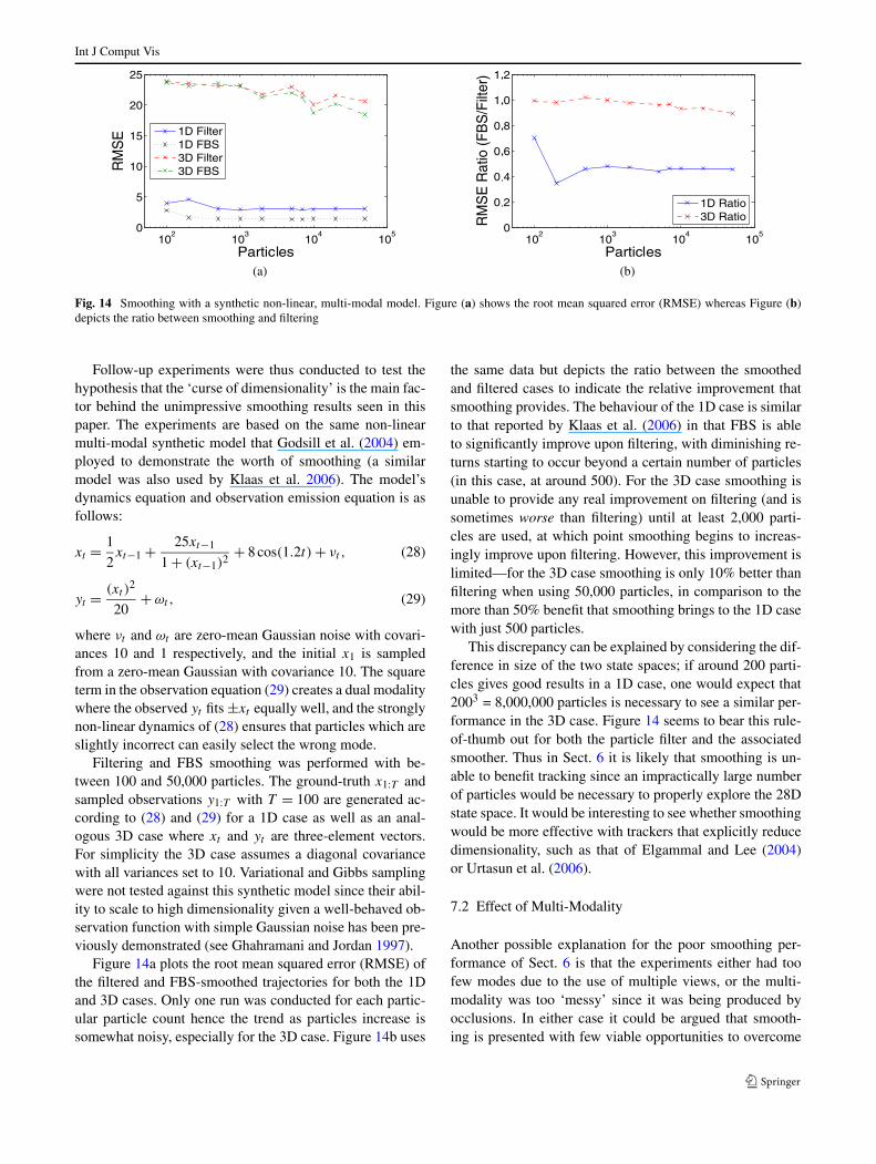
Int J Comput Vis

Fig. 14 Smoothing with a synthetic non-linear, multi-modal model. Figure (a) shows the root mean squared error (RMSE) whereas Figure (b)depicts the ratio between smoothing and filtering

Follow-up experiments were thus conducted to test thehypothesis that the ‘curse of dimensionality’ is the main fac-tor behind the unimpressive smoothing results seen in thispaper. The experiments are based on the same non-linearmulti-modal synthetic model that Godsill et al. (2004) em-ployed to demonstrate the worth of smoothing (a similarmodel was also used by Klaas et al. 2006). The model’sdynamics equation and observation emission equation is asfollows:

xt = 1

2xt−1 + 25xt−1

1 + (xt−1)2+ 8 cos(1.2t) + νt , (28)

yt = (xt )2

20+ ωt , (29)

where νt and ωt are zero-mean Gaussian noise with covari-ances 10 and 1 respectively, and the initial x1 is sampledfrom a zero-mean Gaussian with covariance 10. The squareterm in the observation equation (29) creates a dual modalitywhere the observed yt fits ±xt equally well, and the stronglynon-linear dynamics of (28) ensures that particles which areslightly incorrect can easily select the wrong mode.

Filtering and FBS smoothing was performed with be-tween 100 and 50,000 particles. The ground-truth x1:T andsampled observations y1:T with T = 100 are generated ac-cording to (28) and (29) for a 1D case as well as an anal-ogous 3D case where xt and yt are three-element vectors.For simplicity the 3D case assumes a diagonal covariancewith all variances set to 10. Variational and Gibbs samplingwere not tested against this synthetic model since their abil-ity to scale to high dimensionality given a well-behaved ob-servation function with simple Gaussian noise has been pre-viously demonstrated (see Ghahramani and Jordan 1997).

Figure 14a plots the root mean squared error (RMSE) ofthe filtered and FBS-smoothed trajectories for both the 1Dand 3D cases. Only one run was conducted for each partic-ular particle count hence the trend as particles increase issomewhat noisy, especially for the 3D case. Figure 14b uses

the same data but depicts the ratio between the smoothedand filtered cases to indicate the relative improvement thatsmoothing provides. The behaviour of the 1D case is similarto that reported by Klaas et al. (2006) in that FBS is ableto significantly improve upon filtering, with diminishing re-turns starting to occur beyond a certain number of particles(in this case, at around 500). For the 3D case smoothing isunable to provide any real improvement on filtering (and issometimes worse than filtering) until at least 2,000 parti-cles are used, at which point smoothing begins to increas-ingly improve upon filtering. However, this improvement islimited—for the 3D case smoothing is only 10% better thanfiltering when using 50,000 particles, in comparison to themore than 50% benefit that smoothing brings to the 1D casewith just 500 particles.

This discrepancy can be explained by considering the dif-ference in size of the two state spaces; if around 200 parti-cles gives good results in a 1D case, one would expect that2003 = 8,000,000 particles is necessary to see a similar per-formance in the 3D case. Figure 14 seems to bear this rule-of-thumb out for both the particle filter and the associatedsmoother. Thus in Sect. 6 it is likely that smoothing is un-able to benefit tracking since an impractically large numberof particles would be necessary to properly explore the 28Dstate space. It would be interesting to see whether smoothingwould be more effective with trackers that explicitly reducedimensionality, such as that of Elgammal and Lee (2004)or Urtasun et al. (2006).

7.2 Effect of Multi-Modality

Another possible explanation for the poor smoothing per-formance of Sect. 6 is that the experiments either had toofew modes due to the use of multiple views, or the multi-modality was too ‘messy’ since it was being produced byocclusions. In either case it could be argued that smooth-ing is presented with few viable opportunities to overcome

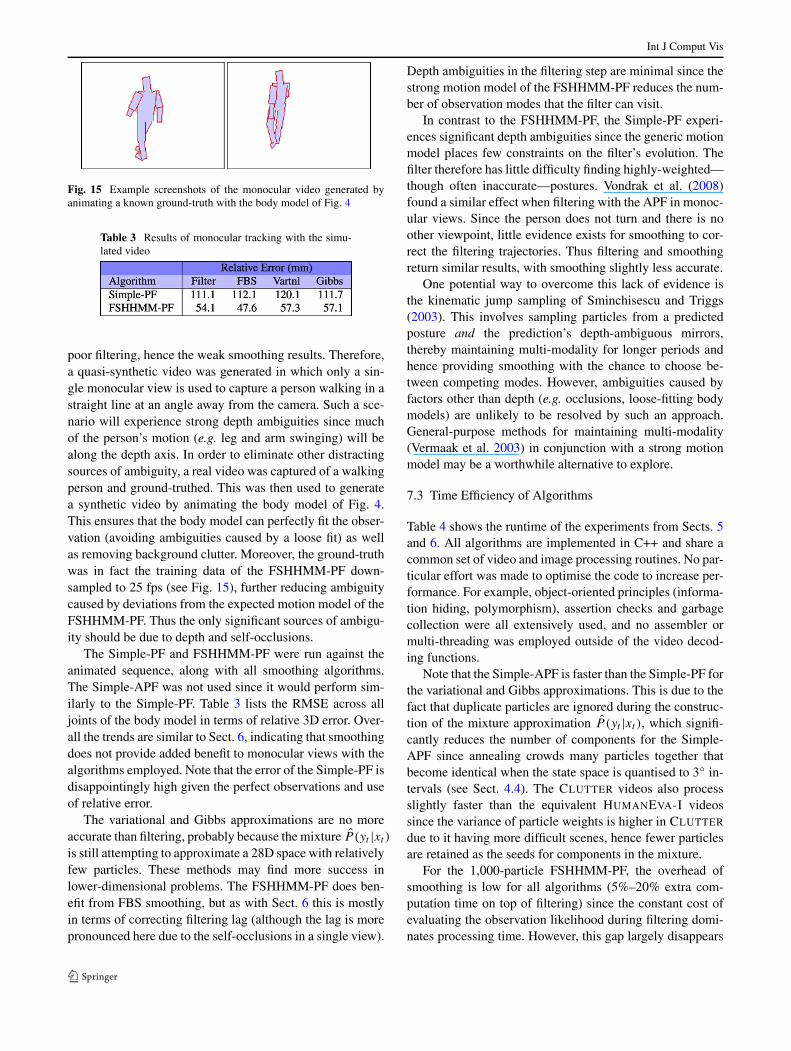
Int J Comput Vis

Fig. 15 Example screenshots of the monocular video generated byanimating a known ground-truth with the body model of Fig. 4

Table 3 Results of monocular tracking with the simu-lated video

poor filtering, hence the weak smoothing results. Therefore,a quasi-synthetic video was generated in which only a sin-gle monocular view is used to capture a person walking in astraight line at an angle away from the camera. Such a sce-nario will experience strong depth ambiguities since muchof the person’s motion (e.g. leg and arm swinging) will bealong the depth axis. In order to eliminate other distractingsources of ambiguity, a real video was captured of a walkingperson and ground-truthed. This was then used to generatea synthetic video by animating the body model of Fig. 4.This ensures that the body model can perfectly fit the obser-vation (avoiding ambiguities caused by a loose fit) as wellas removing background clutter. Moreover, the ground-truthwas in fact the training data of the FSHHMM-PF down-sampled to 25 fps (see Fig. 15), further reducing ambiguitycaused by deviations from the expected motion model of theFSHHMM-PF. Thus the only significant sources of ambigu-ity should be due to depth and self-occlusions.

The Simple-PF and FSHHMM-PF were run against theanimated sequence, along with all smoothing algorithms.The Simple-APF was not used since it would perform sim-ilarly to the Simple-PF. Table 3 lists the RMSE across alljoints of the body model in terms of relative 3D error. Over-all the trends are similar to Sect. 6, indicating that smoothingdoes not provide added benefit to monocular views with thealgorithms employed. Note that the error of the Simple-PF isdisappointingly high given the perfect observations and useof relative error.

The variational and Gibbs approximations are no moreaccurate than filtering, probably because the mixture P (yt |xt )

is still attempting to approximate a 28D space with relativelyfew particles. These methods may find more success inlower-dimensional problems. The FSHHMM-PF does ben-efit from FBS smoothing, but as with Sect. 6 this is mostlyin terms of correcting filtering lag (although the lag is morepronounced here due to the self-occlusions in a single view).

Depth ambiguities in the filtering step are minimal since thestrong motion model of the FSHHMM-PF reduces the num-ber of observation modes that the filter can visit.

In contrast to the FSHHMM-PF, the Simple-PF experi-ences significant depth ambiguities since the generic motionmodel places few constraints on the filter’s evolution. Thefilter therefore has little difficulty finding highly-weighted—though often inaccurate—postures. Vondrak et al. (2008)found a similar effect when filtering with the APF in monoc-ular views. Since the person does not turn and there is noother viewpoint, little evidence exists for smoothing to cor-rect the filtering trajectories. Thus filtering and smoothingreturn similar results, with smoothing slightly less accurate.

One potential way to overcome this lack of evidence isthe kinematic jump sampling of Sminchisescu and Triggs(2003). This involves sampling particles from a predictedposture and the prediction’s depth-ambiguous mirrors,thereby maintaining multi-modality for longer periods andhence providing smoothing with the chance to choose be-tween competing modes. However, ambiguities caused byfactors other than depth (e.g. occlusions, loose-fitting bodymodels) are unlikely to be resolved by such an approach.General-purpose methods for maintaining multi-modality(Vermaak et al. 2003) in conjunction with a strong motionmodel may be a worthwhile alternative to explore.

7.3 Time Efficiency of Algorithms

Table 4 shows the runtime of the experiments from Sects. 5and 6. All algorithms are implemented in C++ and share acommon set of video and image processing routines. No par-ticular effort was made to optimise the code to increase per-formance. For example, object-oriented principles (informa-tion hiding, polymorphism), assertion checks and garbagecollection were all extensively used, and no assembler ormulti-threading was employed outside of the video decod-ing functions.

Note that the Simple-APF is faster than the Simple-PF forthe variational and Gibbs approximations. This is due to thefact that duplicate particles are ignored during the construc-tion of the mixture approximation P (yt |xt ), which signifi-cantly reduces the number of components for the Simple-APF since annealing crowds many particles together thatbecome identical when the state space is quantised to 3◦ in-tervals (see Sect. 4.4). The CLUTTER videos also processslightly faster than the equivalent HUMANEVA-I videossince the variance of particle weights is higher in CLUTTER

due to it having more difficult scenes, hence fewer particlesare retained as the seeds for components in the mixture.

For the 1,000-particle FSHHMM-PF, the overhead ofsmoothing is low for all algorithms (5%–20% extra com-putation time on top of filtering) since the constant cost ofevaluating the observation likelihood during filtering domi-nates processing time. However, this gap largely disappears

Int J Comput Vis

Table 4 Average runtimes per frame for filtering andsmoothing algorithms. HUMANEVA-I video consists ofthree camera views at 640×480 whereas CLUTTER videocomprises four views 384×284 (this only affects filteringruntime since smoothing does not use the video). Experi-ments were run on an Intel Core-2 6420 2.13 GHz

with the 10,000-particle Simple-PF and Simple-APF. Eventhe variational approximation becomes a significant fractionof the filtering time due to the increased number of mixturecomponents that the 10,000 particles generate. Although thesmoothing efficiency is better than one would expect giventhat particle filtering is generally seen as being quite efficient(Klaas et al. 2006), the fact that smoothing does not improveaccuracy makes it difficult to recommend, at least with thefiltering algorithms explored in this paper.

8 Conclusions

This paper has presented a study of three smoothed-inferencealgorithms (forward-backward smoothing, variational andGibbs sampling) for 3D human body tracking in genera-tive models. As part of the study, a method was introducedto facilitate the efficient execution of the latter two algo-rithms by approximating the observation likelihood with amixture of Gaussians. Although it is generally expected thatsmoothing will improve upon the filtering estimate sincesmoothing incorporates future evidence, results in a multi-view environment show that the smoothing algorithms pro-vide no real improvement on the tracking accuracy of fil-tering and in fact can produce an increased error. Simula-tions with monocular views indicate that the same issuesexist in single views despite depth ambiguities being a clas-sic case of multi-modality that smoothing should be wellsuited to handling. The cause of the poor performance ofsmoothing can be traced to the high-dimensional nature of

body tracking—as with earlier studies, smoothing on a low-dimensional signal is shown to significantly improve uponfiltering, but when the dimensionality is increased then ex-ponentially more particles are needed to support effectivesmoothing. In the high-dimensional state space of humanposture this would require an impractically large number ofparticles. Thus for the filtering algorithms explored in thispaper, smoothing does not significantly improve body track-ing accuracy and the time spent on smoothing would bebetter spent on increasing the number of particles for filter-ing. Methods to overcome the difficulties facing smoothingin high-dimensional human body tracking are needed in or-der to take advantage of the benefits that smoothing can giveduring times of poor or ambiguous observations. In additionto investigating new approaches to smoothing and methodsto maintain multi-modality in the filter, a more immediatepossibility is to apply forward-backward particle smoothingto dimensionality-reducing body trackers, sidestepping theproblem of high dimensionality altogether.

Acknowledgements This research is supported by Australian Re-search Council grant LP0561867. We would also like to thank theanonymous reviewers for their valuable comments and suggestions.

References

Andrieu, C., De Freitas, N., Doucet, A., & Jordan, M. I. (2003). Anintroduction to MCMC for machine learning. Machine Learning,50, 5–43.

Balan, A., Sigal, L., & Black, M. J. (2005). A quantitative evaluationof video-based 3D person tracking. In Proceedings of the jointworkshop on visual surveillance and performance and evaluationof tracking systems (VS-PETS) (pp. 349–356).

Barber, D., & Bishop, C. (1998). Ensemble learning in Bayesianneural networks. In M. Jordan, M. Kearns, & S. Solla (Eds.),Neural Networks and Machine Learning (pp. 215–237). NewYork: Springer.

Brubaker, M., Fleet, D. J., & Hertzmann, A. (2006). Physics-based hu-man pose tracking. In Workshop on evaluation of articulated hu-man motion and pose estimation (EHuM).

Brubaker, M. A., Fleet, D. J., & Hertzmann, A. (2007). Physics-basedperson tracking using simplified lower-body dynamics. In Pro-ceedings of the IEEE conference on computer vision and patternrecognition.

Caillette, F., Galata, A., & Howard, T. (2005). Real-time 3-D humanbody tracking using variable length Markov models. In Proceed-ings of the British machine vision conference (pp. 469–478).

Cheng, S. Y., & Trivedi, M. (2007). Articulated human body pose infer-ence from voxel data using a kinematically constrained Gaussianmixture model. In Workshop on evaluation of articulated humanmotion and pose estimation (EHuM).

Corduneanu, A., & Bishop, C. M. (2001). Variational Bayesian modelselection for mixture distributions. In T. Richardson & T. Jaakkola(Eds.), International conference on artificial intelligence and sta-tistics (pp. 27–34).

Deutscher, J., & Reid, I. (2005). Articulated body motion captureby stochastic search. International Journal of Computer Vision,61(2), 185–205.

Int J Comput Vis

Deutscher, J., Blake, A., & Reid, I. (2000). Articulated body motioncapture by annealed particle filtering. In Proceedings of the IEEEconference on computer vision and pattern recognition (Vol. 2,pp. 126–133).

Doucet, A., Godsill, S., & Andrieu, C. (2000). On sequential Monte-Carlo sampling methods for Bayesian filtering. Statistics andComputing, 10(3), 197–208.

Doucet, A., Godsill, S. J., & West, M. (2002). Monte Carlo filtering andsmoothing with application to time-varying spectral estimation. InProceedings of the international conference on audio, speech andsignal processing (Vol. 2, pp. 701–704).

Elgammal, A., & Lee, C.-S. (2004). Inferring 3D body pose fromsilhouettes using activity manifold learning. In Proceedings ofthe IEEE conference on computer vision and pattern recognition(Vol. 2, pp. 681–688).

Ghahramani, Z., & Jordan, M. I. (1997). Factorial Hidden MarkovModels. Machine Learning, 29, 245–273.

Godsill, S. J., Doucet, A., & West, M. (2004). Monte Carlo smooth-ing for nonlinear time series. Journal of the American StatisticalAssociation, 99(465), 156–168.

Gordon, N., Salmond, D., & Smith, A. (1993). Novel approach tononlinear/non-Gaussian Bayesian state estimation. Radar andSignal Processing, IEE Proceedings-F, 140(2), 107–113.

Gupta, A., Mittal, A., & Davis, L. S. (2007). Constraint integra-tion for efficient multiview pose estimation with self-occlusions.IEEE Transactions on Pattern Analysis and Machine Intelligence,30(3), 493–506.

Hua, G., & Wu, Y. (2007). A decentralized probabilistic approach to ar-ticulated body tracking. Computer Vision and Image Understand-ing, 108(2), 272–283.

Husz, Z., & Wallace, A. (2007). Evaluation of a hierarchical partitionedparticle filter with action primitives. In Workshop on evaluation ofarticulated human motion and pose estimation (EHuM).

Isard, M., & Blake, A. (1998). CONDENSATION—conditional den-sity propagation for visual tracking. International Journal ofComputer Vision, 29(1), 5–28.

Kanaujia, A., Sminchisescu, C., & Metaxas, D. (2007). Semi-supervised hierarchical models for 3D human pose reconstruc-tion. In Proceedings of the IEEE conference on computer visionand pattern recognition.

Klaas, M., Briers, M., de Freitas, N., Doucet, A., Maskell, S., &Lang, D. (2006). Fast particle smoothing: If I had a million par-ticles. In Proceedings of the international conference on machinelearning (pp. 481–488).

Lee, C.-S., & Elgammal, A. (2006). Body pose tracking from uncal-ibrated camera using supervised manifold learning. In Workshopon evaluation of articulated human motion and pose estimation(EHuM).

Lee, M. W., & Nevatia, R. (2005). Integrating component cues for hu-man pose tracking. In Proceedings of the joint workshop on visualsurveillance and performance and evaluation of tracking systems(VS-PETS).

Lee, M. W., Cohen, I., & Jung, S. K. (2002). Particle filter with ana-lytical inference for human body tracking. In IEEE workshop onmotion and video computing (pp. 159–165).

Mikic, I., Trivedi, M., Hunter, E., & Cosman, P. (2001). Articulatedbody posture estimation from multi-camera voxel data. In Pro-ceedings of the IEEE conference on computer vision and patternrecognition (Vol. 1, pp. 455–460).

Moeslund, T., Hilton, A., & Krüger, V. (2006). A survey of advancesin vision-based human motion capture and analysis. Computer Vi-sion and Image Understanding, 104(2), 90–126.

Mündermann, L., Corazza, S., & Andriacchi, T. (2007). Accuratelymeasuring human movement using articulated ICP with soft-jointconstraints and a repository of articulated models. In Proceedingsof the IEEE conference on computer vision and pattern recogni-tion.

Neal, R., & Hinton, G. (1998). A new view of the EM algorithm thatjustifies incremental, sparse and other variants. In M. Jordan (Ed.),Learning in Graphical Models (pp. 355–368). Dordrecht: KluwerAcademic.

Peursum, P. (2006). On the behaviour of the annealed particle filter inrealistic conditions (Technical report). Curtin University of Tech-nology. http://impca.cs.curtin.edu.au/pubs/reports.php.

Peursum, P. (2008). Variational and Gibbs inference for generative hu-man body tracking (Technical report). Curtin University of Tech-nology. http://impca.cs.curtin.edu.au/pubs/reports.php.

Peursum, P., Venkatesh, S., & West, G. (2007). Tracking-as-recognition for articulated full-body human motion analysis. InProceedings of the IEEE conference on computer vision and pat-tern recognition.

Poon, E., & Fleet, D. J. (2002). Hybrid Monte Carlo filtering: Edge-based people tracking. In IEEE workshop on motion and videocomputing.

Sidenbladh, H., Black, M. J., & Fleet, D. J. (2000). Stochastic trackingof 3D human figures using 2D image motion. In Proceedings ofthe European conference on computer vision (pp. 702–718).

Sigal, L., & Black, M. J. (2006). HumanEva: Synchronized video andmotion capture dataset for evaluation of articulated human mo-tion (Technical Report CS-06-08). Brown University.

Sigal, L., Bhatia, S., Roth, S., Black, M. J., & Isard, M. (2004). Track-ing loose-limbed people. In Proceedings of the IEEE conferenceon computer vision and pattern recognition (Vol. 1, pp. 421–428).

Sminchisescu, C., & Jepson, A. (2004). Variational mixture smooth-ing for non-linear dynamical systems. In Proceedings of the IEEEconference on computer vision and pattern recognition (Vol. 2,pp. 608–615).

Sminchisescu, C., & Triggs, B. (2001). Covariance scaled sampling formonocular 3D body tracking. In Proceedings of the IEEE confer-ence on computer vision and pattern recognition (Vol. 1, pp. 447–454).

Sminchisescu, C., & Triggs, B. (2003). Kinematic jump processes formonocular 3D human body tracking. In Proceedings of the IEEEconference on computer vision and pattern recognition (Vol. 2,pp. 69–76).

Sminichisescu, C., Kanaujia, A., & Metaxas, D. (2006). Conditionalmodels for contextual human motion recognition. Computer Vi-sion and Image Understanding, 104, 210–220.

Smith, A. W., & Lovell, B. C. (2006). Measurement function designfor visual tracking applications. In Proceedings of the IEEE inter-national conference on pattern recognition (pp. 789–792).

Stauffer, C., & Grimson, W. E. L. (2000). Learning patterns of activityusing real-time tracking. IEEE Transactions on Pattern Analysisand Machine Intelligence, 22(8), 747–757.

Taycher, L., Shakhnarovich, G., Demirdjian, D., & Darrell, T. (2006).Conditional random people: Tracking humans with CRFs and gridfilters. In Proceedings of the IEEE conference on computer visionand pattern recognition (pp. 222–229).

Urtasun, R., Fleet, D. J., Hertzmann, A., & Fua, P. (2005). Priorsfor people tracking from small training sets. In Proceedings ofthe IEEE international conference on computer vision (Vol. 1,pp. 403–410).

Urtasun, R., Fleet, D. J., & Fua, P. (2006). Temporal motion modelsfor monocular and multiview 3D human body tracking. ComputerVision and Image Understanding, 104, 157–177.

Vermaak, J., Doucet, A., & Pérez, P. (2003). Maintaining multi-modality through mixture tracking. In Proceedings of the IEEEinternational conference on computer vision (pp. 1110–1116).

Vondrak, M., Sigal, L., & Jenkins, O. (2008). Physical simulation forprobabilistic motion tracking. In Proceedings of the IEEE confer-ence on computer vision and pattern recognition.

Winn, J., & Bishop, C. (2005). Variational message passing. Journal ofMachine Learning Research, 6, 661–694.