Finite control set model predictive control for an LCL-filtered ...

Finite control set model predictive control for an LCL-filtered grid-tied inverter with full statusestimations under unbalanced grid voltage

Chen, Xiaotao; Wu, Weimin; Gao, Ning; Liu, Jiahao; Chung, Henry Shu-Hung; Blaabjerg,Frede

Published in:Energies

Published: 01/07/2019

Document Version:Final Published version, also known as Publisher’s PDF, Publisher’s Final version or Version of Record

License:CC BY

Publication record in CityU Scholars:Go to record

Published version (DOI):10.3390/en12142691

Publication details:Chen, X., Wu, W., Gao, N., Liu, J., Chung, H. S-H., & Blaabjerg, F. (2019). Finite control set model predictivecontrol for an LCL-filtered grid-tied inverter with full status estimations under unbalanced grid voltage. Energies,12(14), [2691]. https://doi.org/10.3390/en12142691

Citing this paperPlease note that where the full-text provided on CityU Scholars is the Post-print version (also known as Accepted AuthorManuscript, Peer-reviewed or Author Final version), it may differ from the Final Published version. When citing, ensure thatyou check and use the publisher's definitive version for pagination and other details.

General rightsCopyright for the publications made accessible via the CityU Scholars portal is retained by the author(s) and/or othercopyright owners and it is a condition of accessing these publications that users recognise and abide by the legalrequirements associated with these rights. Users may not further distribute the material or use it for any profit-making activityor commercial gain.Publisher permissionPermission for previously published items are in accordance with publisher's copyright policies sourced from the SHERPARoMEO database. Links to full text versions (either Published or Post-print) are only available if corresponding publishersallow open access.

Take down policyContact [email protected] if you believe that this document breaches copyright and provide us with details. We willremove access to the work immediately and investigate your claim.

Download date: 31/01/2022

https://scholars.cityu.edu.hk/en/publications/finite-control-set-model-predictive-control-for-an-lclfiltered-gridtied-inverter-with-full-status-estimations-under-unbalanced-grid-voltage(dd19718d-685d-44c7-9580-140bab299a3d).html

https://doi.org/10.3390/en12142691

https://scholars.cityu.edu.hk/en/persons/shu-hung-henry-chung(7b2a6609-fc97-4c1d-a0e1-b045373599d5).html



https://scholars.cityu.edu.hk/en/journals/energies(6245a94c-1106-4f9f-8615-dedf2c3fcca1)/publications.html

https://doi.org/10.3390/en12142691

energies

Article

Finite Control Set Model Predictive Control for anLCL-Filtered Grid-Tied Inverter with Full StatusEstimations under Unbalanced Grid Voltage

Xiaotao Chen 1, Weimin Wu 1,*, Ning Gao 1, Jiahao Liu 1, Henry Shu-Hung Chung 2 andFrede Blaabjerg 3

1 Department of Electronic Engineering, Shanghai Maritime University, Shanghai 201306, China2 Department of Electronic Engineering, City University of Hong Kong, Hong Kong 999077, China3 Department of Energy Technology, Aalborg University, DK-9220 Aalborg, Denmark* Correspondence: [email protected]

Received: 14 June 2019; Accepted: 11 July 2019; Published: 13 July 2019��

Abstract: This paper proposes a novel finite control set model predictive control (FCS-MPC) strategywith merely grid-injected current sensors for an inductance-capacitance-inductance (LCL)-filteredgrid-tied inverter, which can obtain a sinusoidal grid-injected current whether three-phase gridvoltages are balanced or not. Compared with the conventional FCS-MPC method, four compositionsare added in the proposed FCS-MPC algorithm, where the grid voltage observer (GVO) andLuenberger observer are combined together to achieve full status estimations (including grid voltage,capacitor voltage, inverter-side current, and grid-injected current), while the sequence extractorand the reference generator are applied to eliminate the double frequency ripples of the active orreactive power, or the negative sequence component (NSC) of the grid-injected current caused by theunbalanced grid voltage. Simulation model and experimental platform are established to verify theeffectiveness of the proposed FCS-MPC strategy, with full status estimations under both balancedand unbalanced grid voltage conditions.

Keywords: finite control set model predictive control (FCS-MPC); full status estimations; gridvoltage observer (GVO); inductance-capacitance-inductance (LCL)-filtered grid-tied inverter;Luenberger observer

1. Introduction

Grid-tied inverters have been widely utilized in distributed generation systems, since they are theinterfaces between DC sources and power grids [1,2]. In regards to the control of grid-tied inverters,besides the classical linear control schemes [3,4], a large number of nonlinear control strategies, suchas model predictive control (including continuous control set model predictive control (CCS-MPC)and finite control set model predictive control (FCS-MPC)), sliding mode control, passivity-basedcontrol [5–7], and so on, were proposed. Among them, the FCS-MPC attracted significant attentions inrecent years, owing to the technique advantages, including no need of the modulator, straightforwardhandling of nonlinearities and constraints, quick dynamic responses, and simple implementation [8–11].

Recently, Falkowski et al. [12] proposed an FCS-MPC method for the inductance-capacitance-inductance (LCL)-filtered grid-tied ac-dc converter, which can damp the oscillations caused by the filterresonance and acquire the high performance of grid currents. However, this FCS-MPC method requiresto measure the inverter-side current, the capacitor voltage grid voltage, and the grid-injected current bysensors, increasing the cost and complexity. Aiming at reducing the number of sensors, many sensorlesscontrol schemes, such as virtual flux [13,14], state observer [15,16], and so on, were widely adopted.

Energies 2019, 12, 2691; doi:10.3390/en12142691 www.mdpi.com/journal/energies

http://www.mdpi.com/journal/energies

http://www.mdpi.com

https://orcid.org/0000-0001-8311-7412

http://dx.doi.org/10.3390/en12142691

http://www.mdpi.com/journal/energies

https://www.mdpi.com/1996-1073/12/14/2691?type=check_update&version=2

Energies 2019, 12, 2691 2 of 22

However, these control schemes are usually designed under the ideal grid voltage condition, and thenegative effects caused by the negative sequence component (NSC) are not considered. Therefore,under the unbalanced grid voltage condition, the feasibilities of current sensorless control schemesneed be further verified [17].

To alleviate the adverse effects of the unbalanced grid voltage, the positive sequence component(PSC) and the NSC of the grid voltages are required to be separated first, and then applied in thecontrol algorithm [18–21]. In [18], for the distributed generation inverter, a flexible reference generatorbased on positive and negative active and reactive powers, was proposed to keep feeding the gridand support the grid voltage under the unbalanced grid voltage condition. In [19], to overcome thedistortion of grid-injected currents caused by the unbalanced grid voltages, Zheng et al. proposedan improved virtual synchronous generator control method with the additional positive-sequencecurrent adjuster, allowing the reference currents to track the positive sequence currents and inhibitingthe negative-sequence components. In [20], Suul et al. proposed a virtual-flux-based methodfor the voltage-sensorless grid synchronization under variable grid frequency and unbalancedvoltage conditions, integrating the functions of frequency-adaptive bandpass filtering, the virtualflux estimation, and the sequence separation into one operation. In [21], Yang et al. proposed asliding-mode grid voltage observer for the voltage-sensorless operation under an unbalanced network,separating the PSC and NSC inherently. The variables of methods proposed in [18,19] are all based onthe full state measurements, while only one kind of sensor is reduced in [20,21]. Note that it is of greatchallenge for the LCL-filtered grid-tied inverter to further reduce the number of sensors, especiallyunder the unbalanced grid voltage condition.

In this paper, a novel FCS-MPC approach for the control of an LCL-filtered grid-tied inverterusing merely grid-injected current sensors under the unbalanced grid voltage condition has beenpresented. The method is based on four observations instead of the state measurements (called fullstatus estimations in this paper). In the proposed method, the inverter-side current, the capacitorvoltage, and the grid-injected current are estimated via the Luenberger observer, while the grid voltageand its quadrature signal are observed by the second order generalized integrator (SOGI)-based GVO.According to the output of the GVO, the PSC and NSC of the estimated grid voltage are separatedto generate the reference of grid-injected current, which are used for the FCS-MPC. The PSC ofthe estimated grid voltage acts as the input of the synchronous reference frame phase-locked loop(SRF-PLL), making the system obtain good estimating accuracy, when the grid frequency varies underunbalanced gird voltage condition. Three different control targets for generating the reference ofgrid-injected current—(1) to eliminate the active power ripple; (2) to eliminate the reactive powerripple; and (3) to achieve the balanced and sinusoidal grid-injected currents—are utilized, and theeffectiveness of the proposed FCS-MPC method is verified via simulations and experiments underboth balanced and unbalanced grid voltage condition.

The rest of this paper is organized as follows. The conventional FCS-MPC method for theLCL-filtered grid-tied inverter is first introduced in Section 2. Then, the theoretical analysis of theproposed FCS-MPC scheme with full status estimations under the unbalanced grid voltage conditionis described in Section 3. Next, the detailed implementation of the proposed FCS-MPC strategy ispresented in Sections 4–6 and demonstrate the simulation and experimental results to verify theeffectiveness of the proposed FCS-MPC algorithm, respectively. Finally, a conclusion is drawn inSection 7.

2. Conventional FCS-MPC Method for LCL-Filtered Grid-Tied Inverter

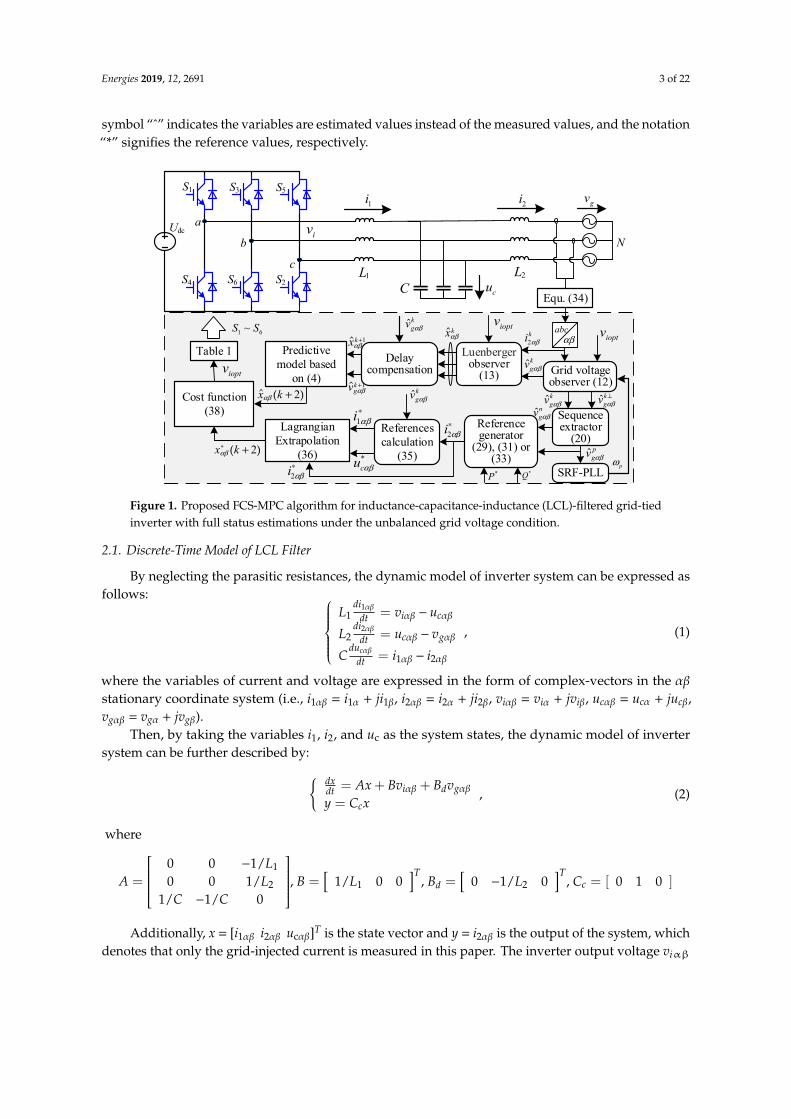
The structure of the three-phase grid-tied inverter with LCL filter powered by a constant DCvoltage source Udc is depicted in Figure 1. As shown in Figure 1, vi, uc, and vg denote the inverteroutput voltage, the capacitor voltage, and the grid voltage, respectively. The currents of i1 and i2represent the inverter-side current and the grid-injected current, respectively. These variables representstate space complex-vectors in the αβ stationary coordinate system, such as vgαβ = vgα + jvgβ. The

Energies 2019, 12, 2691 3 of 22

symbol “ˆ” indicates the variables are estimated values instead of the measured values, and the notation“*” signifies the reference values, respectively.Energies 2019, 12, x FOR PEER REVIEW 3 of 22

Grid voltage observer (12)

S1 S3 S5

S4 S6 S2

Udca

b

c

N

cu

1i 2i

iv

2i αβ∗1i αβ

∗

*cu αβ

References calculation

(35)

Predictive model based

on (4)

Luenberger observer

(13)

Cost function (38)

ˆkgv αβ

2ki αβ

ioptvioptv

gv

Sequence extractor

(20)Reference generator

(29), (31) or (33)

SRF-PLL

Delay compensation

ˆkgv αβ

ˆkgv αβ ˆkgv αβ

*P *Qpω

ˆ pgv αβ

ˆngv αβ

1 6~S S

ˆkgv αβ⊥

Equ. (34)

Lagrangian Extrapolation

(36)

Table 1

ioptv

2i αβ∗

ˆ kxαβ1ˆ kxαβ+

1ˆkgv αβ+

2* ( )x kαβ +

2ˆ ( )x kαβ +

abcαβ

1L 2LC

Figure 1. Proposed FCS-MPC algorithm for inductance-capacitance-inductance (LCL)-filtered grid-tied inverter with full status estimations under the unbalanced grid voltage condition.

2.1. Discrete-Time Model of LCL Filter

By neglecting the parasitic resistances, the dynamic model of inverter system can be expressed as follows:

11

22

1 2

,

αβiαβ cαβ

αβcαβ gαβ

cαβαβ αβ

diL = v - u

dtdi

L = u - vdt

duC = i - i

dt

(1)

where the variables of current and voltage are expressed in the form of complex-vectors in the αβ stationary coordinate system (i.e., i1αβ = i1α + ji1β, i2αβ = i2α + ji2β, viαβ = viα + jviβ, ucαβ = ucα + jucβ, vgαβ = vgα + jvgβ).

Then, by taking the variables i1, i2, and uc as the system states, the dynamic model of inverter system can be further described by:

,

iαβ d gαβ

c

v

y

dx = Ax + B

= C x

v + Bdt (2)

where

1

2

0 0 10 0 1

1 1 0

- / LA = / L ,

/ C - / C [ ]11 0 0 TB = / L , [ ]20 1 ,0 T

dB = - / L [0 1 0]cC =

Additionally, x = [i1αβ i2αβ ucαβ]T is the state vector and y = i2αβ is the output of the system, which denotes that only the grid-injected current is measured in this paper. The inverter output voltage viαβ is obtained by the combinations of switching signals Sa, Sb, Sc, which are described in Table 1, and it can be expressed as a state space complex-vector in αβ stationary reference frame:

Figure 1. Proposed FCS-MPC algorithm for inductance-capacitance-inductance (LCL)-filtered grid-tiedinverter with full status estimations under the unbalanced grid voltage condition.

2.1. Discrete-Time Model of LCL Filter

By neglecting the parasitic resistances, the dynamic model of inverter system can be expressed asfollows:

L1di1αβ

dt = viαβ − ucαβ

L2di2αβ

dt = ucαβ − vgαβ

Cducαβ

dt = i1αβ − i2αβ

, (1)

where the variables of current and voltage are expressed in the form of complex-vectors in the αβstationary coordinate system (i.e., i1αβ = i1α + ji1β, i2αβ = i2α + ji2β, viαβ = viα + jviβ, ucαβ = ucα + jucβ,vgαβ = vgα + jvgβ).

Then, by taking the variables i1, i2, and uc as the system states, the dynamic model of invertersystem can be further described by:{ dx

dt = Ax + Bviαβ + Bdvgαβ

y = Ccx, (2)

where

A =

0 0 −1/L1

0 0 1/L2

1/C −1/C 0

, B =[

1/L1 0 0]T

, Bd =[

0 −1/L2 0]T

, Cc = [ 0 1 0 ]

Additionally, x = [i1αβ i2αβ ucαβ]T is the state vector and y = i2αβ is the output of the system, whichdenotes that only the grid-injected current is measured in this paper. The inverter output voltage viαβ

Energies 2019, 12, 2691 4 of 22

is obtained by the combinations of switching signals Sa, Sb, Sc, which are described in Table 1, and itcan be expressed as a state space complex-vector in αβ stationary reference frame:

viαβ(n) ={

“0”, n = {0 , 7}23 Udce j π3 (n−1), n = {1 , 2 . . . , 6}

. (3)

Table 1. Switching states and voltage vectors.

Sa Sb Sc Voltage Vector

0 0 0 01 0 0 2Udc/31 1 0 Udc/3 + j

√3Udc/3

0 1 0 −Udc/3 + j√

3Udc/30 1 1 −2Udc/30 0 1 −Udc/3− j

√3Udc/3

1 0 1 Udc/3− j√

3Udc/31 1 1 0

For the digital implementation of the control algorithm, the continuous-time dynamic model of theLCL filter can be represented in discrete time (the sampling time is Ts) by adopting the zero-order-hold(ZOH) discretization method:

x(k + 1) = A1x(k) + B1viαβ(k) + B2vgαβ(k), (4)

where matrices A1, B1, B2 are

A1 = eATs , B1 =

∫ Ts

0eAτBdτ, B2 =

∫ Ts

0eAτBddτ.

2.2. Conventional FCS-MPC Scheme

With the improved calculation power, the new generation of the digital signal processor (DSP),the field-programmable gate array (FPGA), and the dSPACE platform were utilized to implementthe computationally-complex control algorithm for power electronics and drives. Consequently, theFCS-MPC method attracted a lot of attention in recent years, since the problem of computationalburden can be preliminary solved. Unlike other linear or nonlinear control methods applied in thegrid-tied inverter, the FCS-MPC algorithm has an obvious advantage of no need of a modulation stage.For the FCS-MPC scheme, by adopting a traversal method (each inverter output voltage vector isused to evaluate a cost function), the inverter output voltage vector with minimum cost function wasselected. Then, the driving signal could be deduced according to Table 1.

For the LCL-filtered grid-tied inverter, the conventional FCS-MPC algorithm was implemented inthe following steps [12]:

1. Measure i1, i2, uc, and vg by using the current and voltage sensors;2. Calculate u∗c and i∗1 according to the given reference of grid-injected current i∗2;

3. Deduce the references of three state variables at next step x∗(k + 1) by utilizing the LagrangianExtrapolation method;

4. Obtain the predictions of three state variables in the next sampling instant x (k + 1) for all possibleinverter output voltage vectors based on the discrete-time model of the LCL filter expressed inEquation (4);

5. Construct the cost function and define the weighting factor;6. Select the optimal inverter output voltage vector by minimizing the cost function;

Energies 2019, 12, 2691 5 of 22

7. Acquire the driving signal according to Table 1.

3. Theoretical Analysis of the Proposed FCS-MPC Scheme with Full Status Estimations underUnbalanced Grid Voltage Condition

For the conventional FCS-MPC algorithm, it requires two kinds of current sensors to measure theinductor currents as well as two types of voltage sensors to probe the capacitor voltages and the gridvoltages, increasing the cost and control complexity. In order to reduce the number of sensors andenhance the control reliability under unbalanced grid voltage condition, a novel FCS-MPC strategy isproposed in this paper. As depicted in Figure 1, compared with the conventional FCS-MPC schemedescribed in Section 2, four compositions including the GVO, the Luenberger observer, the sequenceextractor, and the references generator are added in the proposed FCS-MPC strategy, which can achievefull status estimations and eliminate the negative effects caused by the unbalanced grid voltages. Thedetailed diagram of the proposed strategy is depicted in Figure 2.

Energies 2019, 12, x FOR PEER REVIEW 5 of 22

3. Theoretical Analysis of the Proposed FCS-MPC Scheme with Full Status Estimations under Unbalanced Grid Voltage Condition

For the conventional FCS-MPC algorithm, it requires two kinds of current sensors to measure the inductor currents as well as two types of voltage sensors to probe the capacitor voltages and the grid voltages, increasing the cost and control complexity. In order to reduce the number of sensors and enhance the control reliability under unbalanced grid voltage condition, a novel FCS-MPC strategy is proposed in this paper. As depicted in Figure 1, compared with the conventional FCS-MPC scheme described in Section 2, four compositions including the GVO, the Luenberger observer, the sequence extractor, and the references generator are added in the proposed FCS-MPC strategy, which can achieve full status estimations and eliminate the negative effects caused by the unbalanced grid voltages. The detailed diagram of the proposed strategy is depicted in Figure 2.

ioptv

+

+−

pω

+

+−

2ki αβ

2i αβ⊥

2i αβ

ioptv

ˆioptv⊥

++

+−L1+L2

L1+L2

ˆkgv αβ⊥

ˆkgv αβ

k

k

1/2

/2j ++

+−

ˆ pgv αβ

ˆngv αβ

−

−αβdq

ˆ pgqv

ˆ pgdvPI

fω++ +

pθ

Grid voltage observer Sequence extractor

SRF-PLL

pω

Case1: equation(29) Case2: equation(31) Case3: equation(33)

2i αβ∗

*P*Q

Reference generatorAdaptive filter

Adaptive filterSOGI

SOGI

Figure 2. The block diagram of the proposed strategy under the unbalanced grid voltage condition.

3.1. Grid Voltage Observer

As shown in Figure 2, the adaptive filter consists of the SOGI, the filter gain coefficient k, and the output feedback. It is vital to know the value of the grid angular frequency when the adaptive filter is utilized. In practice, the grid frequency may deviate from the rated value. When assuming that the grid frequency is a constant, the effect of the adaptive filter will drop sharply when the grid frequency shifts, making it difficult to obtain the correct information of the grid voltage. Hence, an approach for detecting the grid frequency is required.

In a three-phase system, the phase lock method of SRF-PLL is usually adopted. Under the ideal grid voltage condition, the SRF-PLL yields great performance and tracks the variable grid frequency accurately. However, under the unbalanced grid voltage condition, the overall dynamic performance of the SRF-PLL would become unacceptably deteriorated, due to the negative effects caused by the unbalanced grid voltages. For handling this problem, a PLL based on the decoupled double synchronous reference frame is utilized [22], which isolates the PSC and NSC of the grid voltages, and then takes the PSC as the input signal of PLL. Additionally, the output grid angular frequency is taken as the input angular frequency of the adaptive filter, making the system achieve the frequency-adaptive under the unbalanced grid voltage condition.

In order to analyze the performance of the adaptive filter on tracking the grid frequency, the transfer functions are expressed as follows:

ˆ1 2 2

p

p p

u kω sG (s) = =u s + kω s +ω

(5)

ˆ 2

2 2 2 ,⊥

p

p p

u kωG (s) = =u s + kω s + ω

(6)

where ωp and k set the center angular frequency and the damping factor of the adaptive filter, respectively. u is the input signal of the adaptive filter, while u and ˆ⊥u are the output signals. The amplitude and phase response of the adaptive filter can be calculated as:

Figure 2. The block diagram of the proposed strategy under the unbalanced grid voltage condition.

3.1. Grid Voltage Observer

As shown in Figure 2, the adaptive filter consists of the SOGI, the filter gain coefficient k, and theoutput feedback. It is vital to know the value of the grid angular frequency when the adaptive filter isutilized. In practice, the grid frequency may deviate from the rated value. When assuming that thegrid frequency is a constant, the effect of the adaptive filter will drop sharply when the grid frequencyshifts, making it difficult to obtain the correct information of the grid voltage. Hence, an approach fordetecting the grid frequency is required.

In a three-phase system, the phase lock method of SRF-PLL is usually adopted. Under the idealgrid voltage condition, the SRF-PLL yields great performance and tracks the variable grid frequencyaccurately. However, under the unbalanced grid voltage condition, the overall dynamic performanceof the SRF-PLL would become unacceptably deteriorated, due to the negative effects caused bythe unbalanced grid voltages. For handling this problem, a PLL based on the decoupled doublesynchronous reference frame is utilized [22], which isolates the PSC and NSC of the grid voltages, andthen takes the PSC as the input signal of PLL. Additionally, the output grid angular frequency is takenas the input angular frequency of the adaptive filter, making the system achieve the frequency-adaptiveunder the unbalanced grid voltage condition.

In order to analyze the performance of the adaptive filter on tracking the grid frequency, thetransfer functions are expressed as follows:

G1(s) =uu=

kωps

s2 + kωps +ω2p

(5)

Energies 2019, 12, 2691 6 of 22

G2(s) =u⊥

u=

kω2p

s2 + kωps +ω2p

, (6)

where ωp and k set the center angular frequency and the damping factor of the adaptive filter,respectively. u is the input signal of the adaptive filter, while u and u⊥ are the output signals. Theamplitude and phase response of the adaptive filter can be calculated as:

∣∣∣G1( jω)∣∣∣ = kωωp√

(kωωp)2+(ω2

p−ω2)

2

∠G1( jω) = arctanω2

p−ω2

kωωp

(7)

{ ∣∣∣G2( jω)∣∣∣ = ωp

ω

∣∣∣G1( jω)∣∣∣

∠G2( jω) = ∠G1( jω) − π2

. (8)

It can be deduced from Equations (7) and (8), if the angular frequency ω of the input signal u isequal to the center angular frequency ωp in the steady state,

∣∣∣G1( jω)∣∣∣ = ∣∣∣G2( jω)

∣∣∣ = 1, ∠G1( jω) = 0,∠G2( jω) = −π/2. Consequently, we can get the conclusion that in combination with the SRF-PLL,although the grid frequency is variable, the adaptive filter can track the input signals accurately withoutany error in the steady state. And, the output signals are a pair of orthogonal quantities, where u and uare in same phase, but u⊥ is 90◦ lag respect to the input signal u.

For the LCL-filtered grid-tied inverter system, due to the high impedance of the filtering capacitorat low frequency, the current of this capacitor can be neglected. When neglecting the current of thefiltering capacitor, the continue-time model of grid-tied inverter with LCL filter in αβ coordinate systemcan be expressed as follows: [

vgα

vgβ

]=

[viαviβ

]− (L1 + L2)

ddt

[i2αi2β

]. (9)

Since the differential of the sinusoidal signal can be transformed into the in-phase or invertedvalue of its quadrature signal, based on the adaptive filter, Equation (9) can be written in the followingform: [

vgα

vgβ

]=

[vioptαvioptβ

]+ωp(L1 + L2)

i⊥2αi⊥2β

(10)

vgαvgβ

= v⊥ioptα

v⊥ioptβ

−ωp(L1 + L2)

[i2αi2β

]. (11)

And then, Equations (10) and (11) can be simplified as follows: vgαβ = vioptαβ +ωp(L1 + L2)i⊥2αβv⊥gαβ = v⊥ioptαβ −ωp(L1 + L2)i2αβ

, (12)

where vgαβ, v⊥gαβ represent the outputs of the GVO (i.e., the estimated grid voltage and its quadrature

signal, respectively). vioptαβ, v⊥ioptαβ and i2αβ, i⊥2αβ are the outputs of the adaptive filter, whose inputsignals are viopt and i2, respectively.

3.2. Luenberger Observer

To further reduce the number of sensors, the Luenberger observer is adopted to combine with theGVO, where the inverter-side current sensors and the capacitor voltage sensors can be saved.

Energies 2019, 12, 2691 7 of 22

The state-space model of the Luenberger observer in the discrete-time domain can be described asfollows: {

x(k + 1) = A1x(k) + B1viopt(k) + B2vg(k) + L(y(k) − y(k))y(k) = Ccx(k)

, (13)

where L = [l1 l2 l3]T represents the observer gain vector and Cc = [0 1 0] is the output vector, whichdenotes that the grid-injected current is measured in this paper. The grid voltage vg is observedby using GVO. By defining the estimation error of ∆x(k) = x(k) − x(k), based on Equation (13), thedynamics of state observation error is derived as:

∆x(k + 1) = x(k + 1) − x(k + 1) = (A1 − LCc)∆x(k). (14)

Hence, if the matrix of A1-LCc is Hurwitz, the error vector will converge to zero. The observability

matrix is full rank (rank[ Cc CcA1 CcA21 ]

T= 3), which indicates that the system is observable.

Therefore, the eigenvalues of the observer can be assigned arbitrarily, and the characteristic polynomialof the observer can be set as:

det(zI −A1 + LCc) = (z− p1)(z− p2)(z− p3), (15)

where p1, p2, and p3 are the desired poles of the Luenberger observer. In order to obtain the values of L,p1, p2, and p3 need to be ensured. It is usually easier to identify the poles first in the s-domain and thenmap them to the z-domain via z = exp(sTs). In the s-domain, the closed-loop characteristic polynomialcan be described as (s + αod)(s2 + 2ζorωors +ω2

or). Then, the poles p1, p2, and p3 in the z-domain can beexpressed as follows: p1 = exp(−αodTs)

p2,3 = exp[(−ζor ± j√

1− ζ2or)ωorTs]

, (16)

where the pair of complex-conjugate poles, determined by ζor and ωor, are set to decide the dominantdynamics of the estimation errors. The real pole αod is located at a higher frequency. ζor is the dampingratio, usually set as 0.707. The range of the natural frequency ωor with respect to the resonancefrequency of LCL filter is regarded from 0.5 to 1, and the value of αod is five to 10 times larger than thepair of complex-conjugate poles.

Hence, the gain vector L can be deduced by solving Equation (15). A common method to solveEquation (15) is utilizing the MATLAB function (i.e., acker). When the observer gain vector L isdeduced, three state variables can be estimated to be applied to the conventional FCS-MPC algorithm.Hence, the inverter-side current sensors and capacitor voltage sensors can be saved. However, sincethe negative effects introduced by the NSC of the unbalanced grid voltage are not considered into thecontrol algorithm, the performance will be deteriorated when the grid voltage falls into unbalance.

3.3. Sequence Extractor

To eliminate the adverse effects caused by the NSC of unbalanced grid voltages, the sequenceextractor of the grid voltages is required.

Under the unbalanced grid voltage condition, by neglecting the zero sequence components, thepositive- and negative-components can be extracted from the grid voltage. Consequently, the gridvoltages, which are estimated by utilizing the GVO in this paper, can be described as the sum of PSCand NSC in αβ reference frame: vgα = vp

gα + vngα = Vp

g cos(ωt + ϕp) + Vng cos(−ωt + ϕn)

vgβ = vpgβ + vn

gβ = Vpg sin(ωt + ϕp) + Vn

g sin(−ωt + ϕn), (17)

Energies 2019, 12, 2691 8 of 22

where vg is the estimated grid voltage and Vg is its amplitude. vpgα, vp

gβ and vngα, vn

gβ are the PSC andNSC of the estimated grid voltage in αβ reference frame, respectively. ϕp and ϕn are the initial phaseangles, and ω is the grid angular frequency.

By utilizing the delayed signal cancellation (DSC) method [23], when the delay time is Tg/4,Equation (17) can be rewritten as: vgα(t− Tg/4) = Vp

g sin(ωt + ϕp) −Vng sin(−ωt + ϕn) = vp

gβ − vngβ

vgβ(t− Tg/4) = −Vpg cos(ωt + ϕp) + Vn

g cos(−ωt + ϕn) = −vpgα + vn

gα. (18)

Hence, according to Equations (17) and (18), the PSC and NSC of the estimated grid voltage canbe deduced in the following equations:

vpgα = 1/2(vgα − vgβ(t− Tg/4))

vpgβ = 1/2(vgα(t− Tg/4) + vgβ)

vngα = 1/2(vgα + vgβ(t− Tg/4))

vngβ = 1/2(−vgα(t− Tg/4) + vgβ)

. (19)

v⊥gα and v⊥gβ are 90◦ lag in respect to vgα and vgβ, respectively, thus they are equivalent to a delay ofTg/4. Then, the Equation (19) can be written as follows based on complex-vectors in the αβ stationarycoordinate system: vp

gαβ = 1/2(vgαβ + jv⊥gαβ)

vngαβ = 1/2(vgαβ − jv⊥gαβ)

. (20)

Hence, based on the GVO, the PSC and NSC of the grid voltage can be deduced, which can beutilized for generating the references of grid-injected currents in the next part.

3.4. Reference Generator

For the unbalanced grid voltages and currents without a zero sequence, the grid voltage andgrid-injected current also can be expressed as the sum of the PSC and NSC in dq reference frame: vg = vp

gαβ + vngαβ = vp

gdqe jωt + vngdqe− jωt

i2 = ip2αβ + in2αβ = ip2dqe jωt + in2dqe− jωt , (21)

where vg is the estimated grid voltage obtained by the GVO. vpgdq and vn

gdq are the PSC and NSC of the

estimated grid voltages in the dq rotating reference system, respectively. Similarly, ip2dq and in2dq are thePSC and NSC of the grid-injected currents in the dq rotating reference system, respectively. ω is thegrid angular frequency.

Based on Equation (21), the power of the grid side can be expressed as follows:

S =32

vgi∗2 =32(vp

gdqe jωt + vngdqe− jωt)(ip2dqe jωt + in2dqe− jωt) = p + jq. (22)

According to Equation (22), the active power of p and reactive power of q can be described as:{p = p0 + pc2 cos(2ωt) + ps2 sin(2ωt)q = q0 + qc2 cos(2ωt) + qs2 sin(2ωt)

, (23)

Energies 2019, 12, 2691 9 of 22

where p0 and q0 are the average values of the active power and reactive power, respectively. pc2, ps2

and qc2, qs2 are ripples of p and q, respectively. As derived in [24], the average value and ripples of pand q can be further expressed as follows:

p0 = 3/2(vpgdip2d + vp

gqip2q + vngdin2d + vn

gqin2q)

pc2 = 3/2(vngdip2d + vn

gqip2q + vpgdin2d + vp

gqin2q)

ps2 = 3/2(vngqip2d − vn

gdip2q − vpgqin2d + vp

gdin2q)

q0 = 3/2(vpgqip2d − vp

gdip2q + vngqin2d − vn

gdin2q)

qc2 = 3/2(vngqip2d − vn

gdip2q + vpgqin2d − vp

gdin2q)

qs2 = 3/2(−vngdip2d − vn

gqip2q + vpgdin2d + vp

gqin2q)

. (24)

The relationship between PSC and NSC of the estimated grid voltage or grid-injected current inthe dq rotating coordinate system and αβ stationary coordinate system is xp

dqxn

dq

= [e− jωt 0

0 e jωt

] xpαβ

xnαβ

, (25)

where x represents the estimated grid voltages or grid-injected currents.By utilizing Equation (25), Equation (24) can be expressed in αβ stationary coordinate system as:

p0 = 3/2(vpgαip2α + vp

gβip2β + vn

gαin2α + vngβi

n2β)

pc2 = 3/2[k1 cos(2ωt) − k2 sin(2ωt)]ps2 = 3/2[k2 cos(2ωt) + k1 sin(2ωt)]q0 = 3/2(vp

gβip2α − vp

gαip2β + vngβi

n2α − vn

gαin2β)

qc2 = 3/2[k3 cos(2ωt) − k4 sin(2ωt)]qs2 = 3/2[k4 cos(2ωt) + k3 sin(2ωt)]

, (26)

where k1 = vn

gαip2α + vngβi

p2β + vp

gαin2α + vpgβi

n2β

k2 = vngβi

p2α − vn

gαip2β − vpgβi

n2α + vp

gαin2βk3 = vn

gβip2α − vn

gαip2β + vpgβi

n2α − vp

gαin2βk4 = −vn

gαip2α − vngβi

p2β + vp

gαin2α + vpgβi

n2β

. (27)

It can be seen from Equations (26) and (27) that if the grid voltages are decided, then the inverterhas four controllable freedoms (ip2α, ip2β, in2α, in2β). This implies that only four control targets can beestablished [25]. Normally, the average values of the active power p0 and reactive power q0 arecontrolled to track their references. Consequently, only the remaining two control freedoms can beselected. According to desired control targets, Equations (26) and (27) can be simplified and solved inthe following three cases also introduced in [17]:

Case 1: To eliminate active power ripples

In this case, the control target is to remove the double frequency ripples of active power (i.e., pc2

and ps2 in Equation (26) are set to zero (Hence, k1, k2 are zero. qc2 and qs2 are uncontrolled and thusthere are reactive power ripples under unbalanced grid voltage. The control objective is equivalent tohandle the following equation:

p0 = P∗

q0 = Q∗

k1 = 0k2 = 0

. (28)

Energies 2019, 12, 2691 10 of 22

Based on Equations (26), (27), and (28), the reference of the grid-injected current can be calculatedas follows: i∗2α

i∗2β

= 2P∗

3[(vpgα)

2+(vp

gβ)2−(vn

gα)2−(vn

gβ)2]

vpgα − vn

gαvp

gβ − vngβ

+ 2Q∗

3[(vpgα)

2+(vp

gβ)2+(vn

gα)2+(vn

gβ)2]

vpgβ + vn

gβ−vp

gα − vngα

, (29)

where i∗2α = ip∗2α + in∗2α, i∗2β = ip∗2β + in∗2β.

Case 2: To eliminate reactive power ripples

In this case, the control target is to eliminate the reactive power ripples (i.e., qc2 and qs2 in Equation(26) are considered as zero). Hence, k3, k4 are both zero. pc2 and ps2 are uncontrolled and thus activepower ripples exist under unbalanced grid voltage conditions. The control objective is equivalent tosolve the following equation:

p0 = P∗

q0 = Q∗

k3 = 0k4 = 0

. (30)

Similarly, based on Equations (26), (27), and (30), the reference of the grid-injected current can beobtained as: i∗2α

i∗2β

= 2P∗

3[(vpgα)

2+(vp

gβ)2+(vn

gα)2+(vn

gβ)2]

vpgα + vn

gαvp

gβ + vngβ

+ 2Q∗

3[(vpgα)

2+(vp

gβ)2−(vn

gα)2−(vn

gβ)2]

vpgβ − vn

gβ−vp

gα + vngα

, (31)

where i∗2α = ip∗2α + in∗2α, i∗2β = ip∗2β + in∗2β.

Case 3: To achieve balanced and sinusoidal grid-injected currents

In this case, the control target is to achieve balanced and sinusoidal grid-injected currents, hence,in2α and in2β are regarded as zero. ip2α and ip2β should be used to satisfy the equations of p0 = P* and q0 =

Q*. Since pc2, ps2 and qc2, qs2 are uncontrolled and thus both active power and reactive power ripplesexist if grid voltages are unbalanced. The control objective is equivalent to deal with the followingequation:

p0 = P∗

q0 = Q∗

in2α = 0in2β = 0

. (32)

According to Equations (26), (27), and (32), the reference of the grid-injected current can bededuced as: i∗2α

i∗2β

= 2P∗

3[(vpgα)

2+ (vp

gβ)2]

vpgα

vpgβ

+ 2Q∗

3[(vpgα)

2+ (vp

gβ)2]

vpgβ−vp

gα

, (33)

where i∗2α = ip∗2α + in∗2α, i∗2β = ip∗2β + in∗2β.A detailed comparison of the proposed FCS-MPC scheme with three different control targets

under unbalanced grid voltage is presented in Table 2.

Energies 2019, 12, 2691 11 of 22

Table 2. A comparison with three different control targets

Case 1 Case 2 Case 3

Double frequency ripples of activepower Not exist Exist Exist

Double frequency ripples ofreactive power Exist Not exist Exist

Grid-injected currents UnbalancedSinusoidal

UnbalancedSinusoidal

BalancedSinusoidal

4. Detailed Implementation of the Proposed FCS-MPC Strategy

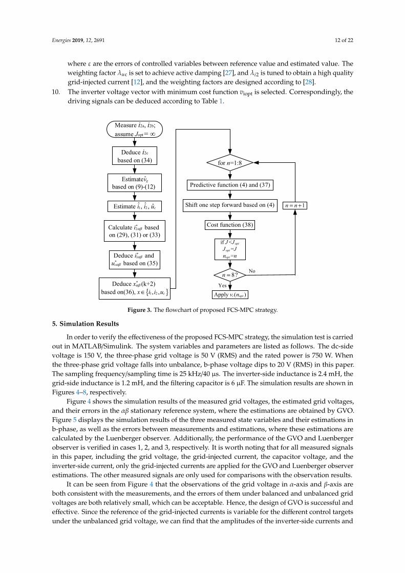
According to the analysis mentioned above, the reference of the grid-injected current can bededuced. Then, it is taken into the FCS-MPC algorithm to alleviate the adverse effects caused by theunbalanced grid voltage. Meanwhile, based on the GVO and Luenberger observer, at least six sensorsare saved. Besides, since the practical implementation of FCS-MPC requires considering the negativeeffect of the computational delay, the discrete-time model of the LCL filter are shifted one step forwardin order to eliminate this time delay (i.e., the values at the (k + 2)th instant rather than the (k + 1)th

instant should be applied in the cost function) [26]. The flowchart of the proposed FCS-MPC algorithmis depicted in Figure 3, where the detailed implementation steps can be summarized as follows:

1. Measure the grid-injected currents of phase a and b, and deduce the c-phase grid-injectedcurrent by

i2c = −(i2a + i2b). (34)

2. Estimate the grid voltage vg by utilizing the GVO based on Equations (9)–(12);3. Estimate the inverter-side inductor current i1, the grid-injected current i2, and the capacitor

voltage uc by using the Luenberger observer, which is based on the observed grid voltages vg andthe measured grid-injected currents;

4. Obtain the reference of grid-injected current i∗2αβ in αβ stationary coordinate system based onEquation (29), (31), or (33);

5. Deduce the references of the inverter-side current i∗1αβ and the capacitor voltage u∗cαβ in αβstationary coordinate system based on i∗2αβ and vgαβ. u∗cαβ = vgαβ −ωL2(i∗2β − ji∗2α)

i∗1αβ = (1−ω2L2C)i∗2αβ. (35)

6. Calculate the references of the three estimated state variables x* at the (k + 2)th instant by utilizingthe Lagrangian extrapolation, which can be expressed as (x = [i1 i2 uc]T):

x∗αβ(k + 2) = 6x∗αβ(k) − 8x∗αβ(k− 1) + 3x∗αβ(k− 2). (36)

7. Predict the three estimated state variables x at the (k + 1)th instant according to Equation (4), andcalculate the estimated grid voltage vg at the (k + 1)th instant by

vg(k + 1) = vg(k)e jωTs . (37)

8. Predict the three estimated state variables x at the (k + 2)th instant, which is based on thediscrete-time model of the LCL filter described in Equation (4);

9. Construct the following cost function and then each voltage vector described in Table 1 is takeninto the cost function. Consequently, seven different value of cost functions J can be obtained.

J = (ε2i1α(k + 2) + ε2

i1β(k + 2)) + λ2i2(ε

2i2α(k + 2) + ε2

i2β(k + 2)) + λ2uc(ε

2ucα(k + 2) + ε2

ucβ(k + 2)), (38)

Energies 2019, 12, 2691 12 of 22

where ε are the errors of controlled variables between reference value and estimated value. Theweighting factor λuc is set to achieve active damping [27], and λi2 is tuned to obtain a high qualitygrid-injected current [12], and the weighting factors are designed according to [28].

10. The inverter voltage vector with minimum cost function viopt is selected. Correspondingly, thedriving signals can be deduced according to Table 1.


2 2 2 2 2 2 21 1 2 2 2( ( 2) ( 2)) ( ( 2) ( 2)) ( ( 2) ( 2)),2

i α i β i i α i β uc ucα ucβJ = ε k + +ε k + +λ ε k+ +ε k + +λ ε k + +ε k + (38)

where ε are the errors of controlled variables between reference value and estimated value. The weighting factor λuc is set to achieve active damping [27], and λi2 is tuned to obtain a high quality grid-injected current [12], and the weighting factors are designed according to [28].

10. The inverter voltage vector with minimum cost function viopt is selected. Correspondingly, the driving signals can be deduced according to Table 1.

for =1:8n

Predictive function (4) and (37)

Shift one step forward based on (4)

Cost function (38)

if <==

opt

opt

opt

J JJ Jn n

8?n =

Yes

No

1n n= +

Apply ( )i optv n

Measure i2a, i2b; assume Jopt = ∞

Deduce i2c based on (34)

ˆEstimate based on (9)-(12)

gv

1 2ˆ ˆ ˆEstimate , , ci i u

*2Calculate based

on (29), (31) or (33)i αβ

*1

*Deduce and

based on (35)c

iu

αβ

αβ

{ }*

1 2

Deduce (k+2) based on(36), , , c

xx i i u

αβ

∈

Figure 3. The flowchart of proposed FCS-MPC strategy.

5. Simulation Results

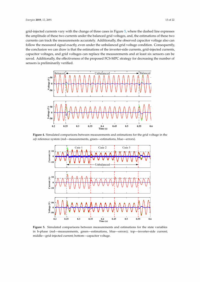
In order to verify the effectiveness of the proposed FCS-MPC strategy, the simulation test is carried out in MATLAB/Simulink. The system variables and parameters are listed as follows. The dc-side voltage is 150 V, the three-phase grid voltage is 50 V (RMS) and the rated power is 750 W. When the three-phase grid voltage falls into unbalance, b-phase voltage dips to 20 V (RMS) in this paper. The sampling frequency/sampling time is 25 kHz/40 μs. The inverter-side inductance is 2.4 mH, the grid-side inductance is 1.2 mH, and the filtering capacitor is 6 μF. The simulation results are shown in Figures 4–8, respectively.

Figure 4 shows the simulation results of the measured grid voltages, the estimated grid voltages, and their errors in the αβ stationary reference system, where the estimations are obtained by GVO. Figure 5 displays the simulation results of the three measured state variables and their estimations in b-phase, as well as the errors between measurements and estimations, where these estimations are calculated by the Luenberger observer. Additionally, the performance of the GVO and Luenberger observer is verified in cases 1, 2, and 3, respectively. It is worth noting that for all measured signals in this paper, including the grid voltage, the grid-injected current, the capacitor voltage, and the inverter-side current, only the grid-injected currents are applied for the GVO and Luenberger observer estimations. The other measured signals are only used for comparisons with the observation results.

It can be seen from Figure 4 that the observations of the grid voltage in α-axis and β-axis are both consistent with the measurements, and the errors of them under balanced and unbalanced grid voltages are both relatively small, which can be acceptable. Hence, the design of GVO is successful and effective. Since the reference of the grid-injected currents is variable for the different control

Figure 3. The flowchart of proposed FCS-MPC strategy.

5. Simulation Results

In order to verify the effectiveness of the proposed FCS-MPC strategy, the simulation test is carriedout in MATLAB/Simulink. The system variables and parameters are listed as follows. The dc-sidevoltage is 150 V, the three-phase grid voltage is 50 V (RMS) and the rated power is 750 W. Whenthe three-phase grid voltage falls into unbalance, b-phase voltage dips to 20 V (RMS) in this paper.The sampling frequency/sampling time is 25 kHz/40 µs. The inverter-side inductance is 2.4 mH, thegrid-side inductance is 1.2 mH, and the filtering capacitor is 6 µF. The simulation results are shown inFigures 4–8, respectively.

Figure 4 shows the simulation results of the measured grid voltages, the estimated grid voltages,and their errors in the αβ stationary reference system, where the estimations are obtained by GVO.Figure 5 displays the simulation results of the three measured state variables and their estimations inb-phase, as well as the errors between measurements and estimations, where these estimations arecalculated by the Luenberger observer. Additionally, the performance of the GVO and Luenbergerobserver is verified in cases 1, 2, and 3, respectively. It is worth noting that for all measured signalsin this paper, including the grid voltage, the grid-injected current, the capacitor voltage, and theinverter-side current, only the grid-injected currents are applied for the GVO and Luenberger observerestimations. The other measured signals are only used for comparisons with the observation results.

It can be seen from Figure 4 that the observations of the grid voltage in α-axis and β-axis areboth consistent with the measurements, and the errors of them under balanced and unbalanced gridvoltages are both relatively small, which can be acceptable. Hence, the design of GVO is successful andeffective. Since the reference of the grid-injected currents is variable for the different control targetsunder the unbalanced grid voltage, we can find that the amplitudes of the inverter-side currents and

Energies 2019, 12, 2691 13 of 22

grid-injected currents vary with the change of three cases in Figure 5, where the dashed line expressesthe amplitude of these two currents under the balanced grid voltages, and, the estimations of these twocurrents can track the measurements accurately. Additionally, the observed capacitor voltage also canfollow the measured signal exactly, even under the unbalanced grid voltage condition. Consequently,the conclusion we can draw is that the estimations of the inverter-side currents, grid-injected currents,capacitor voltages, and grid voltages can replace the measurements and at least six sensors can besaved. Additionally, the effectiveness of the proposed FCS-MPC strategy for decreasing the number ofsensors is preliminarily verified.


targets under the unbalanced grid voltage, we can find that the amplitudes of the inverter-side currents and grid-injected currents vary with the change of three cases in Figure 5, where the dashed line expresses the amplitude of these two currents under the balanced grid voltages, and, the estimations of these two currents can track the measurements accurately. Additionally, the observed capacitor voltage also can follow the measured signal exactly, even under the unbalanced grid voltage condition. Consequently, the conclusion we can draw is that the estimations of the inverter-side currents, grid-injected currents, capacitor voltages, and grid voltages can replace the measurements and at least six sensors can be saved. Additionally, the effectiveness of the proposed FCS-MPC strategy for decreasing the number of sensors is preliminarily verified.

0

50

-50Vol

tage

(V)

0

50

-50Vol

tage

(V)

Time (s)0.25 0.35 0.45 0.550.2 0.3 0.4 0.5 0.6

Balanced BalancedUnbalanced

Figure 4. Simulated comparisons between measurements and estimations for the grid voltage in the αβ reference system (red—measurements, green—estimations, blue—errors).

0

10

-10

0

10

-10

0

50

-50Volta

ge (V

)Cu

rren

t (A

)Cu

rren

t (A

)

Time (s)0.25 0.35 0.45 0.550.2 0.3 0.4 0.5 0.6

Unbalanced

Case 3Case 2Case 1

Figure 5. Simulated comparisons between measurements and estimations for the state variables in b-phase (red—measurements, green—estimations, blue—errors); top—inverter-side current; middle—grid-injected current; bottom—capacitor voltage.

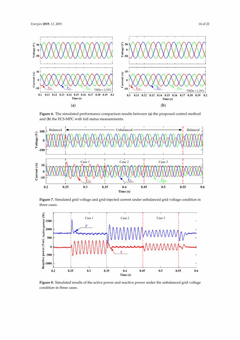
To further verify the effectiveness of the proposed FCS-MPC scheme, the performance comparison results between the proposed control method and the FCS-MPC with full status measurements are displayed in Figure 6. It can be seen that. Compared with the FCS-MPC with full status measurements, the quality of the grid-injected current of the proposed control method declines a little; however, it still can meet the harmonic standard of IEEE (the THD of the grid-injected current

Figure 4. Simulated comparisons between measurements and estimations for the grid voltage in theαβ reference system (red—measurements, green—estimations, blue—errors).


targets under the unbalanced grid voltage, we can find that the amplitudes of the inverter-side currents and grid-injected currents vary with the change of three cases in Figure 5, where the dashed line expresses the amplitude of these two currents under the balanced grid voltages, and, the estimations of these two currents can track the measurements accurately. Additionally, the observed capacitor voltage also can follow the measured signal exactly, even under the unbalanced grid voltage condition. Consequently, the conclusion we can draw is that the estimations of the inverter-side currents, grid-injected currents, capacitor voltages, and grid voltages can replace the measurements and at least six sensors can be saved. Additionally, the effectiveness of the proposed FCS-MPC strategy for decreasing the number of sensors is preliminarily verified.

0

50

-50Vol

tage

(V)

0

50

-50Vol

tage

(V)

Time (s)0.25 0.35 0.45 0.550.2 0.3 0.4 0.5 0.6


Figure 4. Simulated comparisons between measurements and estimations for the grid voltage in the αβ reference system (red—measurements, green—estimations, blue—errors).

0

10

-10

0

10

-10

0

50

-50Volta

ge (V

)Cu

rren

t (A

)Cu

rren

t (A

)

Time (s)0.25 0.35 0.45 0.550.2 0.3 0.4 0.5 0.6

Unbalanced

Case 3Case 2Case 1

Figure 5. Simulated comparisons between measurements and estimations for the state variables in b-phase (red—measurements, green—estimations, blue—errors); top—inverter-side current; middle—grid-injected current; bottom—capacitor voltage.

To further verify the effectiveness of the proposed FCS-MPC scheme, the performance comparison results between the proposed control method and the FCS-MPC with full status measurements are displayed in Figure 6. It can be seen that. Compared with the FCS-MPC with full status measurements, the quality of the grid-injected current of the proposed control method declines a little; however, it still can meet the harmonic standard of IEEE (the THD of the grid-injected current

Figure 5. Simulated comparisons between measurements and estimations for the state variablesin b-phase (red—measurements, green—estimations, blue—errors); top—inverter-side current;middle—grid-injected current; bottom—capacitor voltage.

Energies 2019, 12, 2691 14 of 22


does not exceed 5%). Note that, compared with the FCS-MPC with full status measurements, at least six sensors can be saved for the proposed method.

0.11 0.13 0.15 0.170.1 0.12 0.14 0.16 0.18

0

10

-10

0

-50

Time (s)

Vol

tage

(V)

Cur

rent

(A)

2bi 2ci 2ai THDa 2 34. %=

0.19 0.2

50

0.11 0.13 0.15 0.170.1 0.12 0.14 0.16 0.18

0

10

-10

0

-50

Time (s)

Vol

tage

(V)

Cur

rent

(A)

2bi 2ci 2aiTHDa 1 26. %=

0.19 0.2

50

(a) (b)

Figure 6. The simulated performance comparison results between (a) the proposed control method and (b) the FCS-MPC with full status measurements.

Figure 7 shows the simulation results of the grid voltages and grid-injected currents under balanced and unbalanced grid voltages. The top of Figure 7 depicts that the grid voltages vary from balanced to unbalanced at 0.25 s, and then back to balanced at 0.55 s. In order to achieve grid synchronization and ensure the maximum energy injected into the grid, Q* is set to zero in this paper. Hence, based on Equations (29), (31), and (33), the references of the grid-injected currents can be calculated. The bottom of Figure 7 reveals the performance of the grid-injected currents under the unbalanced grid voltages by utilizing the proposed FCS-MPC strategy based on three different control targets. Figure 8 represents the simulation results of the active power and reactive power under the balanced and unbalanced grid voltages. It can be seen from Figure 7 that the three-phase grid-injected currents are sinusoidal but unbalanced in case 1 and case 2; however, the grid-injected currents are balanced and sinusoidal in case 3. For Figure 8, we found that the double frequency ripples of active power are eliminated in case 1, the double frequency ripples of reactive power are eliminated in case 2, and the double frequency ripples of both the active and reactive power exist in case 3, which is in agreement with the theoretical analysis described in Table 2. Therefore, according to Figures 4–8, it can be verified that the proposed FCS-MPC strategy with merely grid-injected current sensors is effective, and it can obtain good performance of the grid-injected currents even under the unbalanced grid voltage condition.

0.25 0.35 0.45 0.550.2 0.3 0.4 0.5 0.6

0

10

-10

0

100

-100

Time (s)

Vol

tage

(V)

Cur

rent

(A)

2bi 2ci 2ai



Figure 7. Simulated grid voltage and grid-injected current under unbalanced grid voltage condition in three cases.

Figure 6. The simulated performance comparison results between (a) the proposed control methodand (b) the FCS-MPC with full status measurements.


does not exceed 5%). Note that, compared with the FCS-MPC with full status measurements, at least six sensors can be saved for the proposed method.

0.11 0.13 0.15 0.170.1 0.12 0.14 0.16 0.18

0

10

-10

0

-50

Time (s)

Vol

tage

(V)

Cur

rent

(A)

2bi 2ci 2ai THDa 2 34. %=

0.19 0.2

50

0.11 0.13 0.15 0.170.1 0.12 0.14 0.16 0.18

0

10

-10

0

-50

Time (s)

Vol

tage

(V)

Cur

rent

(A)

2bi 2ci 2aiTHDa 1 26. %=

0.19 0.2

50

(a) (b)

Figure 6. The simulated performance comparison results between (a) the proposed control method and (b) the FCS-MPC with full status measurements.

Figure 7 shows the simulation results of the grid voltages and grid-injected currents under balanced and unbalanced grid voltages. The top of Figure 7 depicts that the grid voltages vary from balanced to unbalanced at 0.25 s, and then back to balanced at 0.55 s. In order to achieve grid synchronization and ensure the maximum energy injected into the grid, Q* is set to zero in this paper. Hence, based on Equations (29), (31), and (33), the references of the grid-injected currents can be calculated. The bottom of Figure 7 reveals the performance of the grid-injected currents under the unbalanced grid voltages by utilizing the proposed FCS-MPC strategy based on three different control targets. Figure 8 represents the simulation results of the active power and reactive power under the balanced and unbalanced grid voltages. It can be seen from Figure 7 that the three-phase grid-injected currents are sinusoidal but unbalanced in case 1 and case 2; however, the grid-injected currents are balanced and sinusoidal in case 3. For Figure 8, we found that the double frequency ripples of active power are eliminated in case 1, the double frequency ripples of reactive power are eliminated in case 2, and the double frequency ripples of both the active and reactive power exist in case 3, which is in agreement with the theoretical analysis described in Table 2. Therefore, according to Figures 4–8, it can be verified that the proposed FCS-MPC strategy with merely grid-injected current sensors is effective, and it can obtain good performance of the grid-injected currents even under the unbalanced grid voltage condition.

0.25 0.35 0.45 0.550.2 0.3 0.4 0.5 0.6

0

10

-10

0

100

-100

Time (s)

Vol

tage

(V)

Cur

rent

(A)

2bi 2ci 2ai



Figure 7. Simulated grid voltage and grid-injected current under unbalanced grid voltage condition in three cases. Figure 7. Simulated grid voltage and grid-injected current under unbalanced grid voltage condition inthree cases.Energies 2019, 12, x FOR PEER REVIEW 15 of 22

0

500

1000

1500

-500

-1000

Time (s)

Act

ive p

ower

(W)

Rea

ctiv

e po

wer

(Var

)

0.25 0.35 0.45 0.550.2 0.3 0.4 0.5 0.6


p

q

Figure 8. Simulated results of the active power and reactive power under the unbalanced grid voltage condition in three cases.

6. Experimental Results

To further verify the effectiveness of the proposed FCS-MPC strategy, the laboratory test-rig depicted in Figure 9 is established. The experimental parameters were the same as the simulation ones. The programmable ac source (Chroma 61830) is utilized to simulate the balanced and unbalanced grid voltage condition. The power stage consists of a two-level voltage-source inverter (Danfoss-FC320) with a dc-link voltage provided by Chroma 62150 H-600S DC power supply. The digital control algorithm is implemented in dSPACE 1202 platform, where a control desk project is established to regulate control parameters and reference values, as well as display the experimental results which cannot be probed by the Yokogawa DL 1640 digital oscilloscope assembled with two current probes HIOKI 3276, including the inverter-side currents, grid-injected currents, capacitor voltages, grid voltages, active power, and reactive power in this paper.

Chroma 61830(AC voltage

source)

dSPACE1202

Danfoss-FC320

(Inverter)

Sampling board

Yokogawa DL 1640

(Oscilloscope)

LCL filter HIOKI 3276

(Current probe)

Chroma 62150H-600S (DC voltage source)

PC

.

Figure 9. The experimental test setup.

Figure 10 displays the experimental comparisons between measurements and estimations for the grid voltage in α-axis and β-axis, respectively, when grid voltage varies from unbalanced to balanced based on case 1. Figure 11 shows the experimental comparisons between measurements and estimations for the state variables in b-phase when grid voltage varies from unbalanced to balanced based on case 1. In Figures 10 and 11, the red line expresses the measurement, the green line

Figure 8. Simulated results of the active power and reactive power under the unbalanced grid voltagecondition in three cases.

Energies 2019, 12, 2691 15 of 22

To further verify the effectiveness of the proposed FCS-MPC scheme, the performance comparisonresults between the proposed control method and the FCS-MPC with full status measurements aredisplayed in Figure 6. It can be seen that. Compared with the FCS-MPC with full status measurements,the quality of the grid-injected current of the proposed control method declines a little; however, itstill can meet the harmonic standard of IEEE (the THD of the grid-injected current does not exceed5%). Note that, compared with the FCS-MPC with full status measurements, at least six sensors can besaved for the proposed method.

Figure 7 shows the simulation results of the grid voltages and grid-injected currents underbalanced and unbalanced grid voltages. The top of Figure 7 depicts that the grid voltages varyfrom balanced to unbalanced at 0.25 s, and then back to balanced at 0.55 s. In order to achieve gridsynchronization and ensure the maximum energy injected into the grid, Q* is set to zero in this paper.Hence, based on Equations (29), (31), and (33), the references of the grid-injected currents can becalculated. The bottom of Figure 7 reveals the performance of the grid-injected currents under theunbalanced grid voltages by utilizing the proposed FCS-MPC strategy based on three different controltargets. Figure 8 represents the simulation results of the active power and reactive power under thebalanced and unbalanced grid voltages. It can be seen from Figure 7 that the three-phase grid-injectedcurrents are sinusoidal but unbalanced in case 1 and case 2; however, the grid-injected currents arebalanced and sinusoidal in case 3. For Figure 8, we found that the double frequency ripples of activepower are eliminated in case 1, the double frequency ripples of reactive power are eliminated in case2, and the double frequency ripples of both the active and reactive power exist in case 3, which isin agreement with the theoretical analysis described in Table 2. Therefore, according to Figures 4–8,it can be verified that the proposed FCS-MPC strategy with merely grid-injected current sensors iseffective, and it can obtain good performance of the grid-injected currents even under the unbalancedgrid voltage condition.


To further verify the effectiveness of the proposed FCS-MPC strategy, the laboratory test-rigdepicted in Figure 9 is established. The experimental parameters were the same as the simulation ones.The programmable ac source (Chroma 61830) is utilized to simulate the balanced and unbalanced gridvoltage condition. The power stage consists of a two-level voltage-source inverter (Danfoss-FC320) witha dc-link voltage provided by Chroma 62150 H-600S DC power supply. The digital control algorithm isimplemented in dSPACE 1202 platform, where a control desk project is established to regulate controlparameters and reference values, as well as display the experimental results which cannot be probed bythe Yokogawa DL 1640 digital oscilloscope assembled with two current probes HIOKI 3276, includingthe inverter-side currents, grid-injected currents, capacitor voltages, grid voltages, active power, andreactive power in this paper.

Energies 2019, 12, 2691 16 of 22


0

500

1000

1500

-500

-1000

Time (s)

Act

ive p

ower

(W)

Rea

ctiv

e po

wer

(Var

)

0.25 0.35 0.45 0.550.2 0.3 0.4 0.5 0.6


p

q

Figure 8. Simulated results of the active power and reactive power under the unbalanced grid voltage condition in three cases.


To further verify the effectiveness of the proposed FCS-MPC strategy, the laboratory test-rig depicted in Figure 9 is established. The experimental parameters were the same as the simulation ones. The programmable ac source (Chroma 61830) is utilized to simulate the balanced and unbalanced grid voltage condition. The power stage consists of a two-level voltage-source inverter (Danfoss-FC320) with a dc-link voltage provided by Chroma 62150 H-600S DC power supply. The digital control algorithm is implemented in dSPACE 1202 platform, where a control desk project is established to regulate control parameters and reference values, as well as display the experimental results which cannot be probed by the Yokogawa DL 1640 digital oscilloscope assembled with two current probes HIOKI 3276, including the inverter-side currents, grid-injected currents, capacitor voltages, grid voltages, active power, and reactive power in this paper.

Chroma 61830(AC voltage

source)

dSPACE1202

Danfoss-FC320

(Inverter)

Sampling board

Yokogawa DL 1640

(Oscilloscope)

LCL filter HIOKI 3276

(Current probe)

Chroma 62150H-600S (DC voltage source)

PC


Figure 10 displays the experimental comparisons between measurements and estimations for the grid voltage in α-axis and β-axis, respectively, when grid voltage varies from unbalanced to balanced based on case 1. Figure 11 shows the experimental comparisons between measurements and estimations for the state variables in b-phase when grid voltage varies from unbalanced to balanced based on case 1. In Figures 10 and 11, the red line expresses the measurement, the green line


Figure 10 displays the experimental comparisons between measurements and estimations forthe grid voltage in α-axis and β-axis, respectively, when grid voltage varies from unbalanced tobalanced based on case 1. Figure 11 shows the experimental comparisons between measurements andestimations for the state variables in b-phase when grid voltage varies from unbalanced to balancedbased on case 1. In Figures 10 and 11, the red line expresses the measurement, the green line denotes theestimation, and the blue line represents their error. Additionally, it can be found that the observationstrack the measurements accurately both in steady and dynamic states, reflecting the effectiveness ofthe GVO and Luenberger observer. Therefore, the sensors of inverter-side current, capacitor voltage,and grid voltage can be saved by taking the observations instead of measurements into the FCS-MPCalgorithm. The experimental comparisons based on case 2 and case 3 also can be obtained, and theeffects of track are similar to the case 1, thus it is not shown in this paper. It should be noticed that, forall measurements, except for the grid-injected currents, the other measured signals are merely utilizedfor comparisons with the estimated results.


denotes the estimation, and the blue line represents their error. Additionally, it can be found that the observations track the measurements accurately both in steady and dynamic states, reflecting the effectiven

estimation

measurement

error

Time (s)

Vol

tage

(V)

Unbalanced Balanced

estimationmeasurementerror

Time (s)

Vol

tage

(V)

Unbalanced Balanced

(a) (b)

Figure 10. Experimental comparisons between measurements and estimations for the grid voltage in the αβ reference system when grid voltage varies from unbalanced to balanced in case 1.

estimation

measurementerror

Cur

rent

(A)

Time (s)

Unbalanced Balanced

.0 62.0 6.0 58.0 56.0 54.0 52

estimation

measurement

error

Cur

rent

(A)

Time (s)

Unbalanced Balanced

(a) (b)

estimation

measurementerror

Time (s)

Vol

tage

(V)

Unbalanced Balanced

(c)

Figure 11. Experimental comparisons between measurements and estimations for the state variables in b-phase when grid voltage varies from unbalanced to balanced in case 1: (a) Inverter-side current, (b) grid-injected current, (c) capacitor voltage.

Figure 12 depicts the experimental performance comparison results between the proposed control method and the FCS-MPC with full status measurements. Although the THD of the grid-

Figure 10. Experimental comparisons between measurements and estimations for the grid voltagein the αβ reference system when grid voltage varies from unbalanced to balanced in case 1: (a) Gridvoltage in α-axis, (b) grid voltage in β-axis.

Energies 2019, 12, 2691 17 of 22


denotes the estimation, and the blue line represents their error. Additionally, it can be found that the observations track the measurements accurately both in steady and dynamic states, reflecting the effectiven

estimation

measurement

error

Time (s)

Vol

tage

(V)

Unbalanced Balanced

estimationmeasurementerror

Time (s)

Vol

tage

(V)

Unbalanced Balanced

(a) (b)

Figure 10. Experimental comparisons between measurements and estimations for the grid voltage in the αβ reference system when grid voltage varies from unbalanced to balanced in case 1.

estimation

measurementerror

Cur

rent

(A)

Time (s)

Unbalanced Balanced

.0 62.0 6.0 58.0 56.0 54.0 52

estimation

measurement

error

Cur

rent

(A)

Time (s)

Unbalanced Balanced

(a) (b)

estimation

measurementerror

Time (s)

Vol

tage

(V)

Unbalanced Balanced

(c)

Figure 11. Experimental comparisons between measurements and estimations for the state variables in b-phase when grid voltage varies from unbalanced to balanced in case 1: (a) Inverter-side current, (b) grid-injected current, (c) capacitor voltage.

Figure 12 depicts the experimental performance comparison results between the proposed control method and the FCS-MPC with full status measurements. Although the THD of the grid-

Figure 11. Experimental comparisons between measurements and estimations for the state variables inb-phase when grid voltage varies from unbalanced to balanced in case 1: (a) Inverter-side current, (b)grid-injected current, (c) capacitor voltage.

Figure 12 depicts the experimental performance comparison results between the proposed controlmethod and the FCS-MPC with full status measurements. Although the THD of the grid-injectedcurrent by adopting the proposed control method is higher than the one using the FCS-MPC with fullstatus measurements, the difference between these two THD values of grid-injected current is not solarge, where they both meet the harmonic standard of IEEE (the THD of grid-injected current does notexceed 5%). Therefore, the effectiveness of the proposed control method is verified.


injected current by adopting the proposed control method is higher than the one using the FCS-MPC with full status measurements, the difference between these two THD values of grid-injected current is not so large, where they both meet the harmonic standard of IEEE (the THD of grid-injected current does not exceed 5%). Therefore, the effectiveness of the proposed control method is verified.

THDa 3 20. %=

[70V/div]gv

2[5A/div]iTime:[10ms/div] THDa 2 25. %=

[70V/div]gv

2[5A/div]iTime:[10ms/div]

(a) (b)

Figure 12. The experimental performance comparison results between (a) the proposed control method and (b) the FCS-MPC with full status measurements.

Figures 13–15 show the experimental results of grid-injected currents, active and reactive power by utilizing the proposed FCS-MPC scheme based on three different control targets, which are adopted to eliminate the negative effects caused by the unbalanced grid voltage, respectively. Due to the limitation of the experimental device, only a-phase and b-phase voltages and currents are measured. It can be observed from Figure 13 that the grid-injected currents are sinusoidal but unbalanced (the current in b-phase is largest, while the amplitude of currents in a-phase and c-phase are same) in the steady states, and the dynamic performance is good when the grid voltages vary from balanced to unbalanced and then back to balanced. Note that further optimization in the research is possible by increasing the sampling frequency, but it is not the subject of this paper, and the double frequency ripples of the active power are eliminated, while the ripples of the reactive power still exist under the unbalanced grid voltage. Hence, the experimental results are in agreement with the theoretical analysis of case 1.

[5A/div]Time:[10ms/div] 2i

Balanced Unbalanced

[70V/div]gv

(a)

[70V/div]

[5A/div] Time:[10ms/div]2i

gv

BalancedUnbalanced

(b)

Figure 12. The experimental performance comparison results between (a) the proposed control methodand (b) the FCS-MPC with full status measurements.

Figures 13–15 show the experimental results of grid-injected currents, active and reactive power byutilizing the proposed FCS-MPC scheme based on three different control targets, which are adopted to

Energies 2019, 12, 2691 18 of 22

eliminate the negative effects caused by the unbalanced grid voltage, respectively. Due to the limitationof the experimental device, only a-phase and b-phase voltages and currents are measured. It can beobserved from Figure 13 that the grid-injected currents are sinusoidal but unbalanced (the currentin b-phase is largest, while the amplitude of currents in a-phase and c-phase are same) in the steadystates, and the dynamic performance is good when the grid voltages vary from balanced to unbalancedand then back to balanced. Note that further optimization in the research is possible by increasingthe sampling frequency, but it is not the subject of this paper, and the double frequency ripples of theactive power are eliminated, while the ripples of the reactive power still exist under the unbalancedgrid voltage. Hence, the experimental results are in agreement with the theoretical analysis of case 1.


injected current by adopting the proposed control method is higher than the one using the FCS-MPC with full status measurements, the difference between these two THD values of grid-injected current is not so large, where they both meet the harmonic standard of IEEE (the THD of grid-injected current does not exceed 5%). Therefore, the effectiveness of the proposed control method is verified.

THDa 3 20. %=

[70V/div]gv

2[5A/div]iTime:[10ms/div] THDa 2 25. %=

[70V/div]gv

2[5A/div]iTime:[10ms/div]

(a) (b)

Figure 12. The experimental performance comparison results between (a) the proposed control method and (b) the FCS-MPC with full status measurements.

Figures 13–15 show the experimental results of grid-injected currents, active and reactive power by utilizing the proposed FCS-MPC scheme based on three different control targets, which are adopted to eliminate the negative effects caused by the unbalanced grid voltage, respectively. Due to the limitation of the experimental device, only a-phase and b-phase voltages and currents are measured. It can be observed from Figure 13 that the grid-injected currents are sinusoidal but unbalanced (the current in b-phase is largest, while the amplitude of currents in a-phase and c-phase are same) in the steady states, and the dynamic performance is good when the grid voltages vary from balanced to unbalanced and then back to balanced. Note that further optimization in the research is possible by increasing the sampling frequency, but it is not the subject of this paper, and the double frequency ripples of the active power are eliminated, while the ripples of the reactive power still exist under the unbalanced grid voltage. Hence, the experimental results are in agreement with the theoretical analysis of case 1.


Balanced Unbalanced

[70V/div]gv

(a)

[70V/div]


gv

BalancedUnbalanced

(b) Energies 2019, 12, x FOR PEER REVIEW 18 of 22

p

q

Time (s)

Act

ive

po

wer

(W

)R

eact

ive

pow

er (

Var)

Unbalanced Balanced

(c)

Figure 13. Experimental results of (a) grid-injected current when grid voltage varies from balanced to

unbalanced, (b) grid-injected current when grid voltage varies from unbalanced to balanced, and (c)

active and reactive power when grid voltage varies from unbalanced to balanced in case 1.

As demonstrated in Figure 14, the performance of the grid-injected currents are acceptable both

in steady (the current in b-phase is smallest, while the amplitude of currents in a-phase and c-phase

are same) and dynamic states, and the double frequency ripples of the reactive power are eliminated,

while the active power ripples still exist under the unbalanced grid voltage. Consequently, the

experimental results verify the correctness of the theory of case 2.

[70V/div]


gv

Balanced Unbalanced

(a)

[70V/div]


gv

Unbalanced Balanced

(b)

Figure 13. Experimental results of (a) grid-injected current when grid voltage varies from balanced tounbalanced, (b) grid-injected current when grid voltage varies from unbalanced to balanced, and (c)active and reactive power when grid voltage varies from unbalanced to balanced in case 1.

Energies 2019, 12, 2691 19 of 22


p

q

Time (s)

Activ

e pow

er (W

)R

eact

ive p

ower

(Var

)

Unbalanced Balanced

(c)

Figure 13. Experimental results of (a) grid-injected current when grid voltage varies from balanced to unbalanced, (b) grid-injected current when grid voltage varies from unbalanced to balanced, and (c) active and reactive power when grid voltage varies from unbalanced to balanced in case 1.

A

[70V/div]


gv

Balanced Unbalanced

(a)

[70V/div]


gv

Unbalanced Balanced

(b)Energies 2019, 12, x FOR PEER REVIEW 19 of 22

Act

ive p

ow

er

(W)

Rea

ctiv

e p

ow

er (

Va

r)

p

q

Time (s)

Unbalanced Balanced

(c)




Figure 15 displays the sinusoidal grid-injected currents with different amplitudes under the

balanced grid voltage and the unbalanced grid voltage. However, it can be found that the currents

are balanced whether three-phase grid voltages are balanced or not, and the transient performance is

good when the grid voltages change from balanced to unbalanced and then back to balanced.

Furthermore, the double frequency ripples of the active and reactive power are not removed under

the unbalanced grid voltages. These performances are also consistent with the theoretical analysis of

case 3.

[70V/div]


gv

Balanced Unbalanced

(a)

[70V/div]


gv

Unbalanced Balanced

(b)


As demonstrated in Figure 14, the performance of the grid-injected currents are acceptable both insteady (the current in b-phase is smallest, while the amplitude of currents in a-phase and c-phase aresame) and dynamic states, and the double frequency ripples of the reactive power are eliminated, whilethe active power ripples still exist under the unbalanced grid voltage. Consequently, the experimentalresults verify the correctness of the theory of case 2.

Figure 15 displays the sinusoidal grid-injected currents with different amplitudes under thebalanced grid voltage and the unbalanced grid voltage. However, it can be found that the currents arebalanced whether three-phase grid voltages are balanced or not, and the transient performance is goodwhen the grid voltages change from balanced to unbalanced and then back to balanced. Furthermore,

Energies 2019, 12, 2691 20 of 22

the double frequency ripples of the active and reactive power are not removed under the unbalancedgrid voltages. These performances are also consistent with the theoretical analysis of case 3.


Act

ive

pow

er (W

)R

eact

ive p

ower

(Var

)

p

q

Time (s)

Unbalanced Balanced

(c)

Figure 14. Experimental results of (a) grid-injected current when grid voltage varies from balanced to unbalanced, (b) grid-injected current when grid voltage varies from unbalanced to balanced, and (c) active and reactive power when grid voltage varies from unbalanced to balanced in case 2.

Figure 15 displays the sinusoidal grid-injected currents with different amplitudes under the balanced grid voltage and the unbalanced grid voltage. However, it can be found that the currents are balanced whether three-phase grid voltages are balanced or not, and the transient performance is good when the grid voltages change from balanced to unbalanced and then back to balanced. Furthermore, the double frequency ripples of the active and reactive power are not removed under the unbalanced grid voltages. These performances are also consistent with the theoretical analysis of case 3.

[70V/div]


gv

Balanced Unbalanced

(a)

[70V/div]


gv

Unbalanced Balanced

(b)


q

p

Time (s)

Act

ive p

ow

er

(W)

Rea

ctiv

e p

ow

er (

Var)

Unbalanced Balanced

(c)




According to the simulation and experimental results shown above, it can be found that the

proposed FCS-MPC strategy with merely grid-injected current sensors can work well whether the

grid voltages are balanced or not.

7. Conclusions

In this paper, a novel FCS-MPC strategy with full status observations based on GVO and

Luenberger observer is proposed for the LCL-filtered grid-tied inverter under the unbalanced grid

voltage condition. A step-by-step design procedure of the proposed control scheme is described in

detail. The simulation model and experimental platform are established to verify the performance of

proposed control method, where the three different reference cases of the grid-injected currents in

the proposed cost function are analyzed. By theoretical analysis, simulation, and experimental

verification, the following conclusions can be drawn:

1. By utilizing the proposed control algorithm, the errors between observations and measurements

are small enough under both balanced and unbalanced grid voltages, and the observations have

a good dynamic response. Therefore, these observations can replace the measurements used in

the control.

2. Under the unbalanced grid voltage condition, the proposed FCS-MPC strategy obtains the

satisfactory performance in both the steady and dynamic states for three different control targets.

Note that only the grid-injected currents are measured.

Author Contributions: Conceptualization, X.C. and W.W.; methodology, X.C., W.W. and N.G.; software, X.C.

and J.L.; validation, X.C., and N.G.; formal analysis, X.C. and W.W.; investigation, X.C.; resources, W.W.; data

curation, X.C.; writing—original draft preparation, X.C. and W.W.; writing—review and editing, W.W., N.G.,

H.S.C. and F.B.; visualization, X.C.; supervision, W.W., N.G., H.S.C. and F.B.; project administration, W.W.;

funding acquisition, W.W.

Funding: This work was funded in part by the National Natural Science Foundation of China, grant number

51877130 and 51561165013, and in part by the Shanghai Shuguang Talent Program, grant number 14SG43.

Conflicts of Interest: The authors declare no conflicts of interest.

References

1. Blaabjerg, F.; Yang, Y.; Yang, D.; Wang, X. Distributed Power-Generation Systems and Protection. Proc.

IEEE 2017,105, 1311–1331.


According to the simulation and experimental results shown above, it can be found that theproposed FCS-MPC strategy with merely grid-injected current sensors can work well whether the gridvoltages are balanced or not.

Energies 2019, 12, 2691 21 of 22

7. Conclusions

In this paper, a novel FCS-MPC strategy with full status observations based on GVO andLuenberger observer is proposed for the LCL-filtered grid-tied inverter under the unbalanced gridvoltage condition. A step-by-step design procedure of the proposed control scheme is described indetail. The simulation model and experimental platform are established to verify the performance ofproposed control method, where the three different reference cases of the grid-injected currents in theproposed cost function are analyzed. By theoretical analysis, simulation, and experimental verification,the following conclusions can be drawn:

1. By utilizing the proposed control algorithm, the errors between observations and measurementsare small enough under both balanced and unbalanced grid voltages, and the observations havea good dynamic response. Therefore, these observations can replace the measurements used inthe control.

2. Under the unbalanced grid voltage condition, the proposed FCS-MPC strategy obtains thesatisfactory performance in both the steady and dynamic states for three different control targets.Note that only the grid-injected currents are measured.

Author Contributions: Conceptualization, X.C. and W.W.; methodology, X.C., W.W. and N.G.; software, X.C. andJ.L.; validation, X.C., and N.G.; formal analysis, X.C. and W.W.; investigation, X.C.; resources, W.W.; data curation,X.C.; writing—original draft preparation, X.C. and W.W.; writing—review and editing, W.W., N.G., H.S.-H.C.and F.B.; visualization, X.C.; supervision, W.W., N.G., H.S.-H.C. and F.B.; project administration, W.W.; fundingacquisition, W.W.

Funding: This work was funded in part by the National Natural Science Foundation of China, grant number51877130 and 51561165013, and in part by the Shanghai Shuguang Talent Program, grant number 14SG43.

Conflicts of Interest: The authors declare no conflicts of interest.

References

1. Blaabjerg, F.; Yang, Y.; Yang, D.; Wang, X. Distributed Power-Generation Systems and Protection. Proc. IEEE2017, 105, 1311–1331. [CrossRef]

2. Kouro, S.; Leon, J.I.; Vinnikov, D.; Franquelo, L.G. Grid-Connected Photovoltaic Systems: An Overview ofRecent Research and Emerging PV Converter Technology. IEEE Ind. Electron. Mag. 2015, 9, 47–61. [CrossRef]

3. Wu, W.; Liu, Y.; He, Y.; Chung, H.S.; Liserre, M.; Blaabjerg, F. Damping Methods for Resonances Caused byLCL-Filter-Based Current-Controlled Grid-Tied Power Inverters: An Overview. IEEE Trans. Ind. Electron.2017, 64, 7402–7413. [CrossRef]

4. Liu, Y.; Wu, W.; He, Y.; Lin, Z.; Blaabjerg, F.; Chung, H.S. An Efficient and Robust Hybrid Damper for LCL-orLLCL-Based Grid-Tied Inverter with Strong Grid-Side Harmonic Voltage Effect Rejection. IEEE Trans. Ind.Electron. 2016, 63, 926–936. [CrossRef]

5. Ahmed, A.; Koh, B.K.; Lee, Y.I. A Comparison of Finite Control Set and Continuous Control Set ModelPredictive Control Schemes for Speed Control of Induction Motors. IEEE Trans. Ind. Inform. 2018, 14,1334–1346. [CrossRef]

6. Vieira, R.P.; Martins, L.T.; Massing, J.R.; Stefanello, M. Sliding Mode Controller in a Multiloop Frameworkfor a Grid-Connected VSI with LCL Filter. IEEE Trans. Ind. Electron. 2018, 65, 4714–4723. [CrossRef]

7. Mu, X.; Wang, J.; Wu, W.; Blaabjerg, F. A Modified Multifrequency Passivity-Based Control for Shunt ActivePower Filter with Model-Parameter-Adaptive Capability. IEEE Trans. Ind. Electron. 2018, 65, 760–769.[CrossRef]

8. Kouro, S.; Cortes, P.; Vargas, R.; Ammann, U.; Rodriguez, J. Model Predictive Control—A Simple andPowerful Method to Control Power Converters. IEEE Trans. Ind. Electron. 2009, 56, 1826–1838. [CrossRef]

9. Rodriguez, J.; Kazmierkowski, M.P.; Espinoza, J.R.; Zanchetta, P.; Abu-Rub, H.; Young, H.A.; Rojas, C.A.State of the Art of Finite Control Set Model Predictive Control in Power Electronics. IEEE Trans. Ind. Inform.2013, 9, 1003–1016. [CrossRef]

http://dx.doi.org/10.1109/JPROC.2017.2696878

http://dx.doi.org/10.1109/MIE.2014.2376976

http://dx.doi.org/10.1109/TIE.2017.2714143


http://dx.doi.org/10.1109/TII.2017.2758393




http://dx.doi.org/10.1109/TII.2012.2221469

Energies 2019, 12, 2691 22 of 22

10. Yaramasu, V.; Rivera, M.; Wu, B.; Rodriguez, J. Model Predictive Current Control of Two-Level Four-LegInverters—Part I: Concept, Algorithm, and Simulation Analysis. IEEE Trans. Power Electron. 2013, 28,3459–3468. [CrossRef]

11. Xia, C.; Liu, T.; Shi, T.; Song, Z. A Simplified Finite-Control-Set Model-Predictive Control for PowerConverters. IEEE Trans. Ind. Inform. 2014, 10, 991–1002.

12. Falkowski, P.; Sikorski, A. Finite Control Set Model Predictive Control for Grid-Connected AC–DC Converterswith LCL Filter. IEEE Trans. Ind. Electron. 2018, 65, 2844–2852. [CrossRef]

13. Liang, J.; Wang, H.; Yan, Z. Grid Voltage Sensorless Model based Predictive Power Control of PWM RectifiersBased on Sliding Mode Virtual Flux Observer. IEEE Access 2019, 7, 24007–24016. [CrossRef]

14. Zhang, H.; Zhu, X.; Shi, J.; Tan, L.; Zhang, C.; Hu, K. Study on PWM Rectifier Without Grid Voltage SensorBased on Virtual Flux Delay Compensation Algorithm. IEEE Trans. Power Electron. 2019, 34, 849–862.[CrossRef]

15. Yoon, S.; Lai, N.; Kim, K. A Systematic Controller Design for a Grid-Connected Inverter with LCL FilterUsing a Discrete-Time Integral State Feedback Control and State Observer. Energies 2018, 11, 437. [CrossRef]

16. Kukkola, J.; Hinkkanen, M. State Observer for Grid-Voltage Sensorless Control of a Converter Equippedwith an LCL Filter: Direct Discrete-Time Design. IEEE Trans. Ind. Appl. 2016, 52, 3133–3145. [CrossRef]

17. Yang, H.; Zhang, Y.; Liang, J.; Liu, J.; Zhang, N.; Walker, P.D. Robust Deadbeat Predictive Power Control witha Discrete-Time Disturbance Observer for PWM Rectifiers Under Unbalanced Grid Conditions. IEEE Trans.Power Electron. 2019, 34, 287–300. [CrossRef]

18. Camacho, A.; Castilla, M.; Miret, J.; Borrell, A.; de Vicuña, L.G. Active and Reactive Power Strategies withPeak Current Limitation for Distributed Generation Inverters During Unbalanced Grid Faults. IEEE Trans.Ind. Electron. 2015, 62, 1515–1525. [CrossRef]

19. Zheng, X.; Wang, C.; Pang, S. Injecting positive-sequence current virtual synchronous generator controlunder unbalanced grid. IET Renew. Power Gener. 2019, 13, 165–170. [CrossRef]

20. Suul, J.A.; Luna, A.; Rodriguez, P.; Undeland, T. Voltage-Sensor-Less Synchronization to Unbalanced Gridsby Frequency-Adaptive Virtual Flux Estimation. IEEE Trans. Ind. Electron. 2012, 59, 2910–2923. [CrossRef]

21. Yang, H.; Zhang, Y.; Liang, J.; Gao, J.; Walker, P.D.; Zhang, N. Sliding-Mode Observer Based Voltage-SensorlessModel Predictive Power Control of PWM Rectifier Under Unbalanced Grid Conditions. IEEE Trans. Ind.Electron. 2018, 65, 5550–5560. [CrossRef]

22. Rodriguez, P.; Pou, J.; Bergas, J.; Candela, J.I.; Burgos, R.P.; Boroyevich, D. Decoupled Double SynchronousReference Frame PLL for Power Converters Control. IEEE Trans. Power Electron. 2007, 22, 584–592. [CrossRef]

23. Svensson, J.; Bongiorno, M.; Sannino, A. Practical Implementation of Delayed Signal Cancellation Methodfor Phase-Sequence Separation. IEEE Trans. Power Deliv. 2007, 22, 18–26. [CrossRef]

24. Zhou, D.; Tu, P.; Tang, Y. Multivector Model Predictive Power Control of Three-Phase Rectifiers with ReducedPower Ripples Under Nonideal Grid Conditions. IEEE Trans. Ind. Electron. 2018, 65, 6850–6859. [CrossRef]

25. Ma, K.; Chen, W.; Liserre, M.; Blaabjerg, F. Power Controllability of a Three-Phase Converter with anUnbalanced AC Source. IEEE Trans. Power Electron. 2015, 30, 1591–1604. [CrossRef]

26. Chen, X.; Wu, W.; Gao, N.; He, Y.; Chung, H.S.; Blaabjerg, F. Finite Control Set Model Predictive Control forLCL-Filter-Based Grid-Tied Inverter with Computational Delay Compensation. In Proceedings of the 2018IEEE International Power Electronics and Application Conference and Exposition (PEAC), Shenzhen, China,4–7 November 2018; pp. 1–6.

27. Panten, N.; Hoffmann, N.; Fuchs, F.W. Finite Control Set Model Predictive Current Control for Grid-ConnectedVoltage-Source Converters with LCL Filters: A Study Based on Different State Feedbacks. IEEE Trans. PowerElectron. 2016, 31, 5189–5200. [CrossRef]

28. Cortes, P.; Kouro, S.; Rocca, B.L.; Vargas, R.; Rodriguez, J.; Leon, J.I.; Vazquez, S.; Franquelo, L.G. Guidelinesfor weighting factors design in Model Predictive Control of power converters and drives. In Proceedings ofthe 2009 IEEE International Conference on Industrial Technology, Gippsland, Australia, 10–13 February 2009;pp. 1–7.

© 2019 by the authors. Licensee MDPI, Basel, Switzerland. This article is an open accessarticle distributed under the terms and conditions of the Creative Commons Attribution(CC BY) license (http://creativecommons.org/licenses/by/4.0/).

http://dx.doi.org/10.1109/TPEL.2012.2227509


http://dx.doi.org/10.1109/ACCESS.2019.2898687


http://dx.doi.org/10.3390/en11020437

http://dx.doi.org/10.1109/TIA.2016.2542060



http://dx.doi.org/10.1049/iet-rpg.2018.5047




http://dx.doi.org/10.1109/TPWRD.2006.881469




http://creativecommons.org/

http://creativecommons.org/licenses/by/4.0/.

Finite control set model predictive control for an LCL-filtered ...

Documents

Transcript of Finite control set model predictive control for an LCL-filtered ...