A time-domain feedback analysis of filtered-error adaptive gradient algorithms

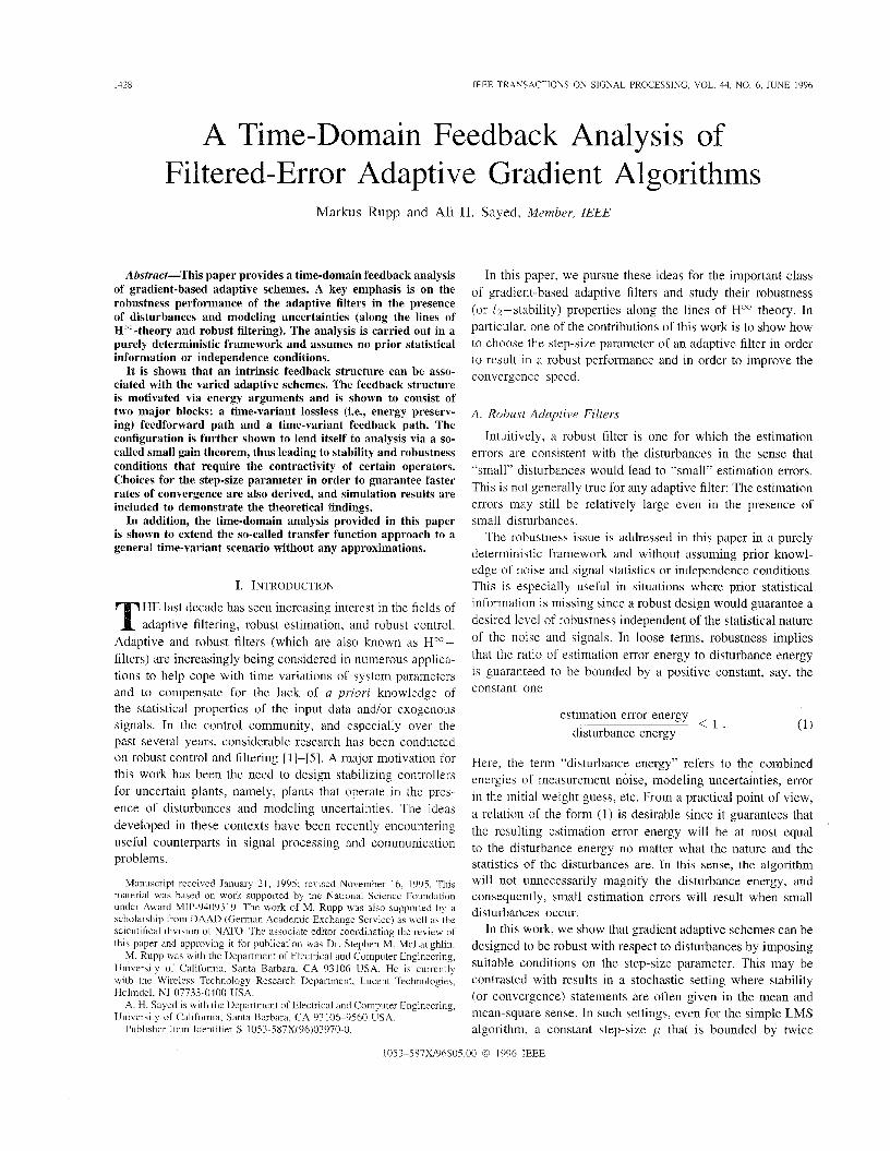
1428 IEEE TRAKSACTIONS ON SIGNAL. PROCESSING, VOL. 44, NO 6, JUNE 1996

e-Domain Feedback Analysis of nor Adaptive Gradient Algorithms

Markus Rupp and Ali H. Sayed, Member, IEEE

Absiruct-This paper provides a time-domain feedback analysis of gradient-based adaptive schemes. A key emphasis is on the robustness performance of the adaptive filters in the presence of disturbances and modeling uncertainties (along the lines of H”-theory and robust filtering). The analysis is carried out in a purely deterministic framework and assumes no prior statistical information or independence conditions.

It is shown that an intrinsic feedback structure can be associated with the varied adaptive schemes. The feedback structure is motivated via energy arguments and is shown to consist of two major blocks: a time-variant lossless (i.e., energy preserving) feedforward path and a time-variant feedback path. The configuration is further shown to lend itself to analysis via a so- called small gain theorem, thus leading to stability and robustness conditions that require the contractivity of certain operators. Choices for the step-size parameter in order to guarantee faster rates of convergence are also derived, and simulation results are included to demonstrate the theoretical findings.

In addition, the time-domain analysis provided in this paper is shown to extend the so-called transfer function approach to a general time-variant scenario without any approximations.

I. INTRODUCTION

HE last decade has seen increasing interest in the fields of adaptive filtering, robust estimation, and robust control.

Adaptive and robust filters (which are also known as H”- filters) are increasingly being considered in numerous applications to help cope with time variations of system parameters and to compensate for the lack of a priori knowledge of the statistical properties of the input data andor exogenous signals. In the control community, and especially over the past several years, considerable research has been conducted on robust control and filtering [1]-[5]. A major motivation for this work has been the need to design stabilizing controllers for uncertain plants, namely, plants that operate in the presence of disturbances and modeling uncertainties. The ideas developed in these contexts have been recently encountering useful counterparts in signal processing and communication problems.

Manuscript received January 21, 1995; revised November 16, 1995. Thls inaterial was based on work supported by the National Sciencc Foundation under Award MIP-9409319. The work of M. Rupp was also supported by a scholarship from DAAD (German Academic Exchange Service) as well as the scientifical division of NATO. The associate editor coordinating the review of this paper and approving it for publication was Dr. Stephen M. McLaughlin.

M. Rupp was with the Department of Electrical and Computer Engineering. University of California. Santa Barbara, CA 93106 USA. He is currenily with the Wireless Technology Research Department, Lucent Technologies. Holmdel, NJ 07733-0400 USA.

A. H. Sayed is with the Department of Electrical and Computer Engineering, University of California, Santa Barbara, CA 93 106-9560 USA.

Publishcr Item Identifier S 1053-58773(96)03970-0.

In this paper, we pursue these ideas for the important class of gradient-based adaptive filters and study their robustness (or /*-stability) properties along the lines of H” theory. In particular, one of the contributions of this work is to show how to choose the step-size parameter of an adaptive filter in order to result in a robust performance and in order to improve the convergence speed.

A. Robust Adaptive Filters

Intuitively, a robust filter is one for which the estimation errors are consistent with the disturbances in the sense that “small” disturbances would lead to “small” estimation errors. This is not generally true for any adaptive filter: The estimation errors may still be relatively large even in the presence of small disturbances.

The robustness issue is addressed in this paper in a purely deterministic framework and without assuming prior knowledge of noise and signal statistics or independence conditions. This is especially useful in situations where prior statistical information is missing since a robust design would guarantee a desired level of robustness independent of the statistical nature of the noise and signals. In loose terms, robustness implies that the ratio of estimation error energy to disturbance energy is guaranteed to be bounded by a positive constant, say, the constant one

estimation error energy disturbance energy 51

Here, the term “disturbance energy” refers to the combined energies of measurement noise, modeling uncertainties, error in the initial weight guess, etc. From a practical point of view, a relation of the form (1) is desirable since it guarantees that the resulting estimation error energy will be at most equal to the disturbance energy no matter what the nature and the statistics of the disturbances are. In this sense, the algorithm will not unnecessarily magnify the disturbance energy, and consequently, small estimation errors will result when small disturbances occur.

In this work, we show that gradient adaptive schemes can be designed to be robust with respect to disturbances by imposing suitable conditions on the step-size parameter. This may be contrasted with results in a stochastic setting where stability (or convergence) statements are often given in the mean and mean-square sense. In such settings, even for the simple LMS algorithm, a constant step-size / - L that is bounded by twice

1053-587W96505 00 0 1996 IEEE

RUPP AND SAYED: TIME-DOMAIN FEEDBACK ANALYSIS OF ADAPTIVE GRADIENT ALGORITHMS 1429

the inverse of the maximal eigenvalue of the autocorrelation matrix can still lead to blow up in a practical experiment [6].

B. A Time-Domain Feedback Analysis

To address the robustness and convergence issues, this paper develops a time-domain approach that proves to be useful in both the analysis and design of robust estimators. It highlights and exploits an intrinsic feedback structure that can be associated with the gradient adaptive schemes.

Although the feedback nature of adaptive filters has been exploited in earlier places in the literature [7]-[9], the feedback configuration studied in this paper has a different emphasis. It does not only refer to the fact that the update equations can be put into a feedback form (as explained in [lo]) but is instead motivated by energy arguments that also explicitly take into consideration both the effect of the measurement noise and the effect of the uncertainty in the initial guess for the weight vector. These extensions are incorporated into the feedback arguments of this paper because the derivation here is specifically interested in a study of the robustness properties of the adaptive schemes.

The feedback interconnection exhibits several features: Its feedforward mapping is lossless (i.e., energy preserving) while its feedback mapping is either memoryless or dynamic. More- over, both mappings are time variant, and their interconnection lends itself to stability analysis via a so-called small gain theorem, which is a very useful tool in system theory [ I l l , W I .

An interesting fallout of the time-domain analysis of this paper is that it can be regarded as an extension of the transfer function approach that is often used in the analysis of gradient- based recursions (e.g, [13], [14]). The time-domain analysis, however, is shown to avoid the restrictions and limitations that are characteristic of the transfer-function domain.

C. Notation

We use small boldface letters to denote vectors and capital boldface letters to denote matrices. In addition, the symbol “*” denotes Hermitian conjugation (complex conjugation for scalars). The symbol I denotes the identity matrix of appropri- ate dimensions, and the boldface letter 0 denotes either a zero vector or a zero matrix. Finally, the notation llxll denotes the Euclidean norm of a vector. All vectors are column vectors except for the input data vector denoted by U;, which is taken to be a row vector.

11. THE LEAST-MEAN-SQUARE ALGORITHM

One of the most widely used adaptive algorithms is the least-mean-squares (LMS) algorithm [15]. It starts with an initial guess wpl for an unknown M x 1 weight vector w and updates it as follows:

where the {ui} are given nonzero row vectors, the { d ( i ) } are given noisy (or disturbed) measurements of the terms {uiw}, viz., d ( i ) = u;w + w ( z ) , and w; is the weight estimate at iteration i. The factor ~ ( i ) is the step-size parameter (which is allowed to be time variant), and the quantity ~ ( i ) may account for both measurement noise and modeling errors. The difference [ d ( i ) - uiwi-11 is denoted by E,(i).

The following error measures are also useful for our later analysis: w i denotes the difference between the true weight w and its estimate w;, i+i = w - wi, e,(i) denotes the a priori estimation error, e,(i) = U ~ W ; - ~ , and e,(i) denotes the a posteriori estimation error e,(i) = uiw;.

It is straightforward to verify that &( i ) = e,(i) + ~ ( i ) . Moreover, it follows from (2) that W; satisfies

w; = Wi-1 - /!L(i)U5EU(i). (3)

If we further multiply (3) by U; from the left, we obtain the following relation among { e p ( i ) ! ea ( i ) , w ( i ) } :

ep ( i ) = [ 1 - I*.(i)//u;I12 ] e,(i) - F(~)IIULII’ ~ ( i ) . (4)

A. Transfer Function Description of the LMS Algorithm

Before proceeding to the time-domain analysis of this paper, we first review a well-known approach to the analysis of LMS- type recursions that employs the concept of transfer functions

In this method, the input vector U, is assumed to have a shift structure, say, U, = [u( i ) , ..., u(i - M + l)], where the individual entries are further assumed to arise from a sinusoidal excitation U ( i) = C cos( ai), Assuming a constant step-size p, and neglecting the initial condition W-1, the transfer function from the disturbance w ( . ) to the (1 priori estimation error e,(.) can be shown to be approximately (see Appendix A, where E,(x) is the z-transform of e,(.))

WI, ~ 4 1 .

where we have defined ,!l = A. Although easily available in the literature, a derivation of the above result is included in Appendix A in order to highlight some of the restrictions and approximations that are needed to establish (5) . These approximations will be avoided when the time-domain analysis is introduced in later sections. For now, however, we stress the fact that an interesting feedback structure is implied by (5 ) . To clarify this, we define 7 ( 2 ) ,

and use (5) to conclude that

(7)

That is, the transfer function from E ( . ) to e,( .) is allpass. Consequently, the transfer function (5 ) , from v ( i ) to e, (.), can be expressed as a feedback structure with an allpass filter in the forward path and a constant gain in the feedback loop.

E,(z) - - 2-1 - cos(R) V ( z ) z -cos(R) . -

1430 IEEE TKANSACTIONS ON SIGNAL PROCESSING, VOL. 44, NO. 6, JUNE 1996

U

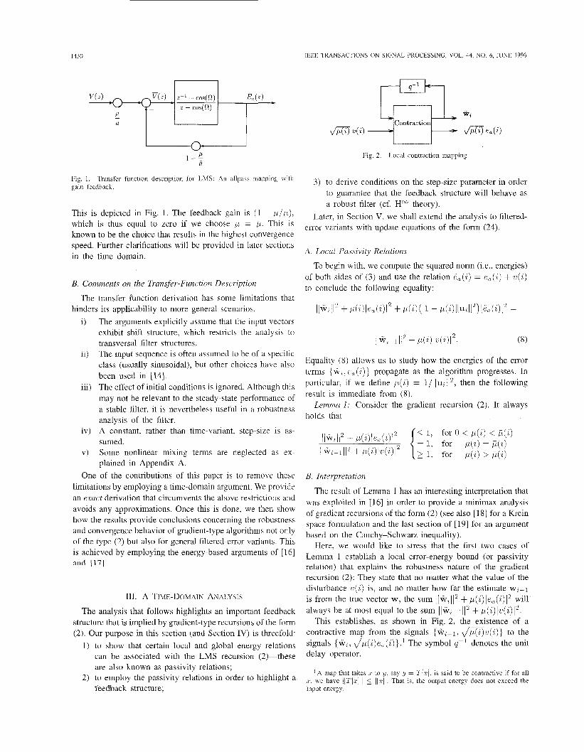
Fig. 2. Local contraction mapping.

Fig. 1. gain feedback.

Transfer function description for LMS: An allpass mapping with 3 ) to derive conditions on the step-size parameter in order to guarantee that the feedback structure will behave as a robust filter (cf. H" theory).

variants with update equations of the

This is depicted in 1. The feedback gain is (l ~ D/D)> Later, in Section V, we shall extend the analysis to filtered- which is thus equal to zero if we choose p = 0. This is known to be the choice that results in the highest convergence speed. Further clarifications will be provided in later sections in the time domain.

(24).

A. Local Passivity Relations

To begin with, we compute the squared norm (i.e., energies) of both sides of (3) and use the relation &( i ) = e,(i) + u ( i ) to conclude the following equality: B. Comments on the Transfer-Function Description

The transfer function derivation has some limitations that hinders its applicability to more general scenarios. I IW;I I~ + p(,i)leo,(i)12 + p ( i ) ( 1 - C L ( ~ ) I I U ~ I I ~ ) I ~ ~ ( ~ ) I ~ =

i)

ii)

iii)

iv)

v)

The arguments explicitly assume that the input vectors exhibit shift structure, which restricts the analysis to transversal filter structures. The input sequence is often assumed to be of a specific class (usually sinusoidal), but other choices have also been used in [14]. The effect of initial conditions is ignored. Although this may not be relevant to the steady-state performance of a stable filter, it is nevertheless useful in a robustness analysis of the filter. A constant, rather than time-variant, step-size is assumed. Some nonlinear mixing terms are neglected as explained in Appendix A.

One of the contributions of this paper is to remove these limitations by employing a time-domain argument. We provide an exact derivation that circumvents the above restrictions and avoids any approximations. Once this is done, we then show how the results provide conclusions concerning the robustness and convergence behavior of gradient-type algorithms not only of the type (2) but also for general filtered-error variants. This is achieved by employing the energy-based arguments of [16] and [17].

111. A TIME-DOMAIN ANALYSIS

The analysis that follows highlights an important feedback structure that is implied by gradient-type recursions of the form (2) . Our purpose in this section (and Section IV) is threefold:

1) to show that certain local and global energy relations can be associated with the LMS recursion (2)-these are also known as passivity relations;

2) to employ the passivity relations in order to highlight a feedback structure;

llwL-ll12 + di)lu(i)12. (8)

Equality (8) allows us to study how the energies of the error terms { W L . e, ( i ) } propagate as the algorithm progresses. In particular, if we define p ( i ) = l / ~ ~ u ~ ~ ~ 2 , then the following result is immediate from (8).

Lemma 1: Consider the gradient recursion (2). It always holds that

B. Interpretation

The result of Lemma 1 has an interesting interpretation that was exploited in 1161 in order to provide a minimax analysis of gradient recursions of the form (2) (see also [ 181 for a Krein space formulation and the last section of [19] for an argument based on the Cauchy-Schwarz inequality).

Here, we would like to stress that the first two cases of Lemma 1 establish a local error-energy bound (or passivity relation) that explains the robustness nature of the gradient recursion (2): They state that no matter what the value of the disturbance ~ ( i ) is, and no matter how far the estimate wi-1

is from the true vector w, the sum ilWi112 + p(i)le,(z)12 will always be at most equal to the sum ~ ~ w ~ - ~ ~ ~ 2 + p(i) lu( i)12.

This establishes, as shown in Fig. 2, the existence of a contractive map from the signals {wi-l, m u ( z ) } to the signals {w?, m e , ( i ) } . ' The symbol qpl denotes the unit delay operator.

' A map that takes x to y, say = T[,r], is said to be contractive if' for all x, we have ilT[.c.]lI 5 11x11. That is, the output energy does not exceed thc input energy.

KUPP AND SAYED: TIME-DOMAIN FEEDBACK ANALYSIS OF ADAPTIVE GRADIENT ALGORITHMS 1431

C. A Global Contraction Mapping

Since the contractivity relation of Fig. 2 holds for each time instant i , it should also hold globally over an interval of time. Indeed, if p( i ) 5 p ( i ) for all i in the interval 0 5 i 5 N , then for all such i (cf. Lemma 1)

ih(i,)Iea(i)12 I I I *~ -~ I I~ - i/will2 + P ( ~ ) I ~ ( ~ I I ~ .

Summing over i , we conclude that N

i=O i = O

This relation states that the map from the disturbances

to the estimation errors

is a contraction. In other words, assume we stack the entries of (10) into a column vector, the entries of (1 1) into a second column vector, and let I& denote the mapping that maps the first vector (10) to the second vector (1 1). The entries of this mapping can be determined from the update relation (3) and from the definition of the a priori estimation error e, (.). The specific values of these entries are not of immediate interest here except to say that it can be verified that IN turns out to be a block lower triangular operator of the form

z v

(For example, the first block entry of TN, which relates e,(0) to w-1, can be easily seen to be m u o ) . The contractivity of z v means that its maximum singular value is at most one,

Inequality (9) is a desirable robustness property in the sense that it guarantees that if the disturbance energy is small, then the resulting estimation error energy will be accordingly small.

We may add that other similar local, and global, passivity relations can be established by using a posteriori (rather than a priori) estimation errors [16]. This is useful in the study of (robust) adaptive IIR filters [20], but we forgo the details here.

c r ( 7 & 7 ) 5 1.

IV. THE FEEDBACK STRUCTURE

The bounds in Lemma 1 can be described via an alternative form that will lead us to an interesting feedback structure. The structure will be shown to constitute the proper extension of the transfer function description of Fig. 1 to the general time- variant scenario, and it will further allow us i) to relax the condition on p ( i ) in order to guarantee robustness and ii) to select p(! i ) for faster speeds of convergence.

We have argued above that if the step sizes are chosen such that ,U(%) 5 $ i ) , then robustness (or contractivity) is

I 0;(4 I

1-- F ( z )

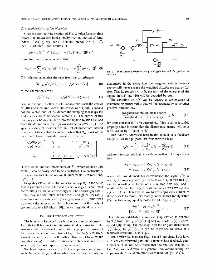
Fig. 3. Time-variant lossless mapping with gain feedback for gradient algorithms.

guaranteed in the sense that the weighted estimation-error energy will never exceed the weighted disturbance energy (cf. (9)). That is, for p(%) 5 p( i ) , the ratio of the energies of the signals in (1 1) and (10) will be bounded by one.

The condition on p( i ) can be relaxed at the expense of guaranteeing energy ratios that will be bounded by some other positive number, say

(12) weighted estimation error energy

weighted disturbance energy I K

for some constant K (to be determined). This is still a desirable property since it means that the disturbance energy will be at most scaled by a factor of K .

This issue is addressed here in the context of a feedback analysis. For this purpose, we first rewrite (4) as

and use it to conclude that (2) can be rewritten in the equivalent form

w, = W,-I + p( i )u:[ea( i ) - e,(i)] = w,-1 + p(i)u:[e , ( i ) + ~ ( i ) ] (14)

where we have defined, for convenience, the signal V ( i ) = - e p ( i ) . Comparing with (2), expression (14) shows that (2) can be rewritten in terms of a new step size p ( i ) and a modified “noise” term V ( z ) (recall that in (2), we have &( i ) = e,(i) + ~ ( i ) ) . Therefore, if we follow arguments similar to those prior to Lemma 1, we readily conclude that for algorithm (2) , the following equality holds for all {p ( i ) , ~ ( i ) } :

This relation establishes a lossless map (which is denoted by Ti) from {wip1, mw(i)} to {wi, m e a ( i ) ] - . Corre- spondingly, using (13), the map from the original disturbance m w ( i ) to m e , ( i ) can be expressed in terms of a feedback structure, as in Fig. 3.

The similarities between Figs. 1 and 3 are clear. Both have a lossless feedforward path and a memoryless feedback path. However, it should be stressed that the analysis that led to Fig. 3 is exact and valid in a general time-variant setting. No approximations or assumptions were made on {ui, PI:^)}.

1432

A. 12-Stability and the Small Gain Theorem

Now that we have introduced the feedback structure of Fig. 3, we can discuss conditions on the step-size parameter p ( i ) in order to guarantee robustness according to (12) for some K .

For this purpose, we start by noting that the feedback configuration of Fig. 3 lends itself rather immediately to stability analysis via tools that are by now standard in system theory, as we explain in the sequel.

It follows from (15) that for every i and for any p( i ) , we have

This allows us to conclude, under a suitable condition on p( a ) , that the system in Fig. 3 is 12-stable, i.e., it maps a bounded energy sequence { w (.)} to a bounded energy sequence {m e,( . )} in a sense precised in (17) below. In fact, we shall also conclude that a similar result will hold even if we replace p(.) with p( . ) (cf. (18)).

Define

That is, A(N) is the maximum absolute value of the gain of the feedback loop over the interval of time 0 I Z I 2v. Likewise, y(N) is the maximum value of the scaling factor p( i ) /p(z) at the input of the feedback interconnection.

Theorem I : Consider the gradient-recursion (2), define A ( N ) and y ( N ) as above, and let p(Z) = l/llui112. If 0 < p ( i ) < 2, i i ( i ) , then the map from {W-l ; w(.)} to {m e,( . )} is L-stable in the following sense:

~

below by a positive quantity for sufficiently large z

Likewise, the map from {w-l, U ( . ) } to {2/1.0 e , ( . ) } (i.e., with p(.) replaced by p( . ) ) is also /*-stable in the following sense:

IEEE TRANSACTIONS ON SIGNAL PROCESSING, VOL. 44, NO. 6, JUNE 1996

Proof: The proof is based on the triangle inequality of

Note that the upper bound on p( i ) is now 2,G(i), which is equivalent to requiring A(N) < 1. This is, in fact, a manifestation of the so-called small gain theorem in system analysis [ l l ] , [12]. In simple terms, the theorem states that the 12 -stability of a feedback configuration (that includes Fig. 3 as a special case) requires that the product of the norms of the feedforward and the feedback operators be strictly bounded by one. Here, the feedforward map has (2-induced) norm equal to one (due to its losslessness), whereas the 2-induced norm of the feedback map is A(N).

The fact that the inequalities in Theorem 1 are valid even for p ( i ) in the interval p ( i ) I p ( i ) < 2 p ( i ) suggests that a local bound, along the lines of Lemma 1, should also exist for this interval. In fact, this is also the case, as shown in the following statement (the derivation is given in Appendix C).

Lemma 2: Given recursion (2), the following holds for

norms and is given in Appendix B.

p ( i ) 5 p ( i ) < 2 p ( i ) :

Before proceeding further, it will be convenient to introduce a matrix notation for later use: Define

N - M.\- = diag { / ~ ( i ) } ~ = ~ , MN = diag {p(i)},”o (19)

and (col( ,) denotes a column vector of its arguments)

It is easy to see that A(N) and y ( N ) are equal to the 2-induced norms of MAv and MN, respectively. The condition A ( N ) < 1 then amounts to requiring the (memoryless) feedback map (I ~ MNM, ) to be contractive.

1

B. A Deterministic Convergence Analysis

In order to further appreciate the significance of the (robustness) bounds of Theorem 1, we now exhibit a convergence analysis that is derived in a purely deterministic setting and without statistical assumptions.

It follows from (3) that w, satisfies

where we have introduced the notation ut. & ( i ) , 4 ( i ) in order to incorporate the factors m. We further introduce the following two deterministic conditions on {6( i ) , ut}:

Finite noise energy: The sequence { li (.)} is assumed to have finite energy, i.e., ~ ~ o p ( i ) 1 u ( z ) / 2 < 30.

Persistent excitation: The rows {U2} are assumed to be persistently exciting. By this, we mean that there exists a finite integer L 2 M such that the smallest singular value of col(U,. . . . , U,+L} is uniformly bounded from

i)

ii)

RUPP AND SAYED: TIME-DOMAIN FEEDBACK ANALYSIS OF ADAPTJVE GRADIENT ALGORITHMS

In the proof of the next statement, we employ the quantities

a = sup 11 - p ( * i ) / p ( i ) l ; y = sup [ p ( i ) / p ( i ) ] i 1

Theorem 2: Assume p(i)lluill* is uniformly bounded by 2 and Iw-111 < CO. If { i j ( s ) } has finite energy, then & ( i ) + 0. If {ui} is further persistently exciting, then w; + w.

Proo) If {6(.)} has finite energy, then (18), for N -+ 00,

implies that { e a ( . ) } also has finite energy. This is true since y < 2, and A < 1. We therefore conclude that { E a ( . ) } is a Cauchy sequence, and hence, & ( i ) + 0.

For the second statement of the theorem, we use (21) to write

i + k - 1

wi = W i + k : - l + U;(&&) + .;(P)). p=i+l

Multiplying from the left by u i + k for k = 1,. . . , L: we get

i t k - 1

k + k W i = &( i + k ) + ui+ku;(ea(p) + 6 ( p ) ) . p=i+l

From the finite noise-energy assumption ( G ( i ) + 0) and the fact that & ( i ) 4 0, we conclude that the right-hand side vanishes as i - m, and hence

[Aui; l ] w; + 0.

Ui+L+l

From the definition of persistent excitation, it follows that wi + 0.

Another point of interest is to note that a related limiting result can be given for finite-power noise sequences {li(.)} (rather than finite-energy), i.e., for w( .) satisfying

1=0

For this purpose, we divide both sides of (18) by take the limit as N --f m to conclude that

and

In other words, a bounded noise power leads to a bounded estimation error power. We may also add that the conclusion of Theorem 2 is in agreement with the result in [21, pp. 140-1431 for the noiseless and constant step-size case.

C. Energy Propagation in the Feedback Cascade

More physical insights into the convergence behavior of the gradient recursion (2) can be obtained by studying the energy flow through the feedback configuration of Fig. 3.

Indeed, let us ignore the measurement noise w ( i ) and assume that we have noiseless measurements d ( i ) = u,w. It is known in the stochastic setting that for Gaussian processes [22], as well as for spherically invariant random processes [23], the maximal speed of convergence is obtained for p(z) = p ( i ) ,

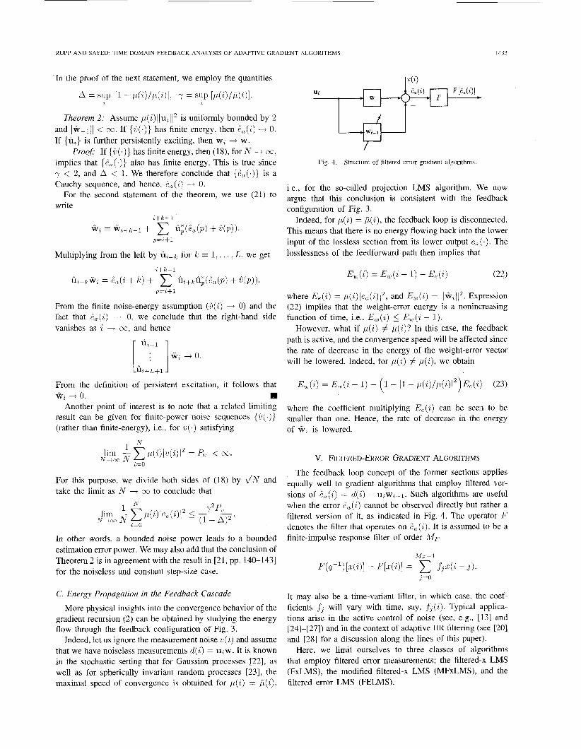
I Fig. 4. Structure of filtercd-error gradient algorithms.

i.e., lor the so-called projection LMS algorithm. We now argue that this conclusion is consistent with the feedback configuration of Fig. 3.

Indeed, for p ( z ) = p ( i ) , the feedback loop is disconnected. This means that there is no energy flowing back into the lower input of the lossless section from its lower output e,(.). The losslessness of the feedforward path then implies that

where Ee(i) = fi(i)lecL(i)12, and & ( i ) = ~ ~ W ~ \ ~ z . Expression (22) implies that the weight-error energy is a nonincreasing function of time, i.e., Eul(i) 5 E,(i - 1).

However, what if p( i ) # j i ( i )? In this case, the feedback path is active, and the convergence speed will be affected since the rate of decrease in the energy of the weight-error vector will be lowered. Indeed, for p( i ) # p ( i ) , we obtain

where the coefficient multiplying E,(i) can be seein to be smaller than one. Hence, the rate of decrease in the energy nf w i c lnwprprl

V. FILTERED-ERROR GRADIENT ALGORITHMS

The feedback loop concept of the former sections applies equally well to gradient algorithms that employ filteired versions of & ( i ) = d ( i ) - u,w,-1. Such algorithms are useful when the error e“, ( i ) cannot be observed directly but rather a filtered version of it, as indicated in Fig. 4. The operator F denotes the filter that operates on Fa(i). It is assumed to be a finite-impulse response filter of order MF

It may also be a time-variant filter, in which case, the coef- ficients f:, will vary with time, say, ,f,(i). Typical applications arise in the active control of noise (see, e.g., [13] and [24]-[27]) and in the context of adaptive IIR filtering (see [20] and [28] for a discussion along the lines of this paper).

Here, we limit ourselves to three classes of algorithms that employ filtered error measurements; the filtered-x LMS (FxLMS), the modified filtered-x LMS (MFxLMS), and the filtered error LMS (FELMS).

1434 I E E t TRANSACTIONS ON SlGNAL PROCESSING, VOL. 44, NO. 6, JUNE 1996

A. The Filtered-x LMS Algorithm C. The Filtered-Error LMS Algorithm

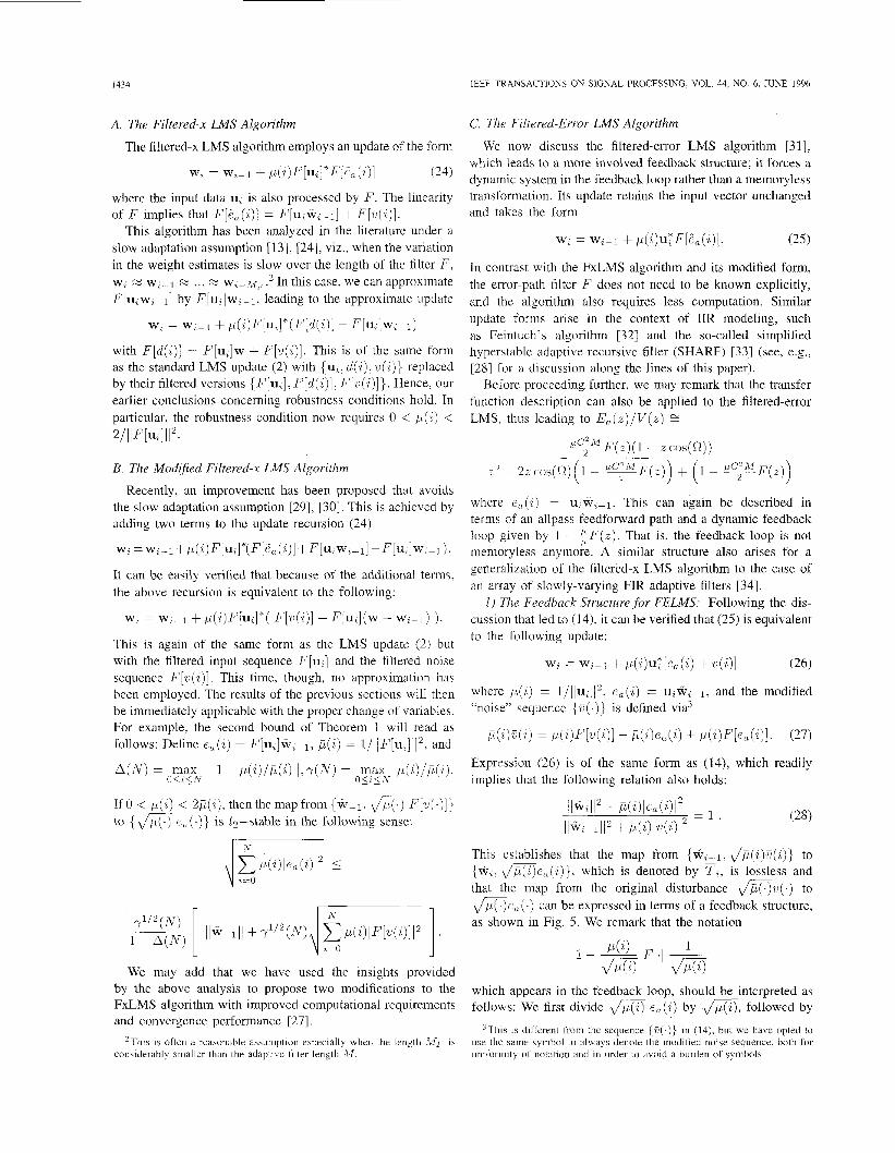
We now discuss the filtered-error LMS algorithm [31], which leads to a more involved feedback structure; it forces a dynamic system in the feedback loop rather than a memoryless transformation. Its update retains the input vector unchanged and takes the form

The filtered-x LMS algorithm employs an update of the form

(24)

where the input data U, is also processed by F . The linearity of F implies that F[P,(i)] = F[u;W;-l] + F[? i ( i ) ] .

This algorithm has been analyzed in the literature under a slow adaptation assumption [13], [24], viz., when the variation in the weight estimates is Slow over the length of the filter F, Wi E Wi-i ... GZ W i - i ~ ~ .* In this case, we can approximate F[U,W,-1] by F [ u ~ j w i - i ~ leading to the approximate update

wz = wz-1 + p( i )F[ui]*F[exa( i ) ]

(25) W? = wi-1 + p( i )u ;F[&( i ) ] .

In contrast with the FxLMS algorithm and its modified form, the error-path filter F does not need to be known explicitly, and the algorithm also requires less computation. Similar update forms arise in the context of IIR modeling, such as Feintuch's algorithm [32] and the so-called simplified hyperstable adaptive recursive filter (SHARF) [33] (see, e.g., [2X] for a discussion along the lines of this paper).

Before proceeding further, we may remark that the transfer function description can also be applied to the filtered-euor LMS, thus leading to E,jz)/V(x) G

w, = w;-1+ p( i )F[u , ]* (F[d( i ) ] - F[U,]W,_1)

with F [ d ( i ) ] = F[u;]w + F [ w ( a ) ] . This is of the same form as the standard LMS update (2) with {u7. d ( i ) . v ( i ) } replaced by their filtered versions { F [ u i ] , F[d(,i)]; F [ v ( i ) ] } . Hence, our earlier conclusions concerning robustness conditions hold. In particular, the robustness condition now requires 0 < p ( i ) <

B. The Modified Filtered-x LMS Algorithm

Recently, an improvement has been proposed that avoids the slow adaptation assumption [29], [30]. This is achieved by adding two terms to the update recursion (24)

wi = w; - 1 + p( i ) F [Ui] *( F [E , ( a ) ] + F [U? wi- 11 - F [Uz] w,- 1 ) .

It can be easily verified that because of the additional terms. the above recursion is equivalent to the following:

W, wi-1 + p ( i ) F [ u i ] * ( F [ v ( i ) ] + F[ui](w - wL-1) ) .

This is again of the same form as the LMS update (2) but with the filtered input sequence F [ u ; ] and the filtered noise sequence F[v( i ) ] . This time, though, no approximation has been employed. The results of the previous sections will then be immediately applicable with the proper change of variables. For example, the second bound of Theorem 1 will read as follows: Define e a ( i ) = F[u;]w;-l, p ( i ) = l/llF[u1j112, and

If 0 < p ( i ) < 2ji (7) , then the map from {W-1.

to { F[1;( . ) ]}

fa(.)} is /z-stable in the following sense:

We may add that we have used the insights provided by the above analysis to propose two modifications to the FxLMS algorithm with improved computational requirements and convergence performance [27]

'Thir is often d rcdsonable assumption especially when the length 111 is considerably mallcr than the adaptive filter length I1

2'' - 22 cos(S2) (1 - @ p F ( x ) ) + (1 - T F ( z ) ) l rC2M

where e a ( i ) = uiwi-1. This can again be described in terms of an allpass feedforward path and a dynamic feedback loop given by 1 - g F ( z ) . That is, the feedback loop is not memoryless anymore. A similar structure also arises for a generalization of the filtered-x LMS algorithm to the case of an array of slowly-varying FIR adaptive filters [34].

I ) The Feedback Structure for FELMS: Following the discussion that led to (14), it can be verified that (25) is equivalent to the following update:

w, = wi-1 + p ( i ) u ; [ e a ( i ) + v ( i j ] (26)

where b( i ) = 1/llu2//2, e, ( i ) = ~ ~ w i - ~ , and the modified "noise" sequence {U(.)} is defined via3

,L(i)E(i) = p( i )F[w( i )] - ,G(i)ecL(i) + p(z)F[ea( i ) ] . (27)

Expression (26) is of the same form as (14), which readily implies that the following relation also holds:

This establishes that the map from {w?-~, m V ( i ) } to {wz. m e a ( i ) } , which is denoted by T L , is lossless and that the map from the original disturbance m u ( . ) to m p a (.) can be expressed in terms of a feedback structure, as shown in Fig. 5 . We remark that the notation

which appears in the feedback loop, should be interpreted as follows: We first divide m ea(z ) by m, followed by

3This is different from the sequence {U(.)} in (14), but we have opted to use the same symbol to always denote the modified noise sequence, both for uniformity of notation and in order to avoid a burden of symbols.

RUPP AND SAYED TIME-DOMAIN FEEDBACK ANA1,YSIS OF ADAPTIVE GRADIENT ALGORITHMS

Fly =

I435

- f o f l .fo . fz f l f o

. fz fl f o . . . . . . . . .

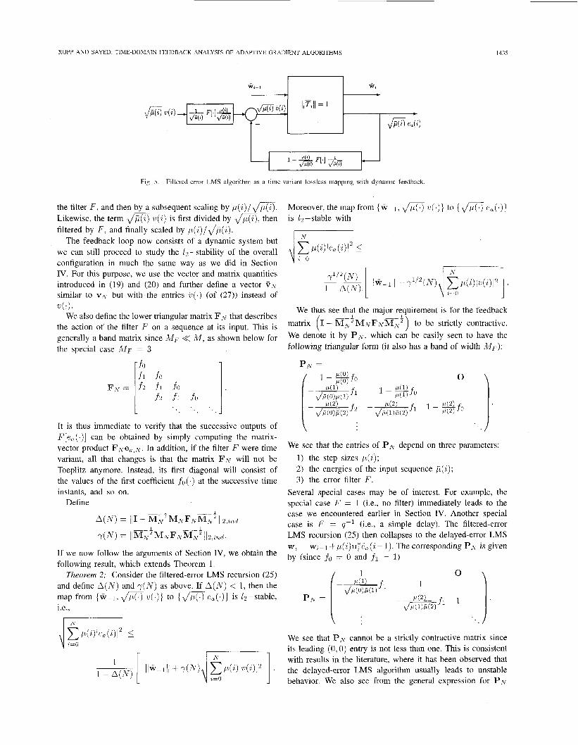
I I I I Fig. 5. Filtered-error LMS algorithm as a time-variant lossless mapping with dynamic feedback.

Moreover, the map from {W-l .

is 12-stable with U ( . ) } to {flJ e , ( . ) }

I N

We thus see that the major requirement is for the feedback

We denote it by P,v, which can be easily seen to have the

-_ - matrix (I - to be strictly contractive.

following triangular form (it also has a band of width Mp):

We see that the entries of P;Y depend on three parameters: 1) the step sizes p(z); 2) the energies of the input sequence J L ( 1 ' ) ; 3) the error filter F .

Several special cases may be of interest. For example, the special case F = 1 (i.e., no filter) immediately leads to the case we encountered earlier in Section IV. Another special case is F = 4-l (i.e., a simple delay). The filtered-error LMS recursion (25) then collapses to the delayed-enor LMS w, = w,-~$,u( i )~~*E,(~- 1). The corresponding P A r is given by (since f o = 0 and f l = I)

1 = f1 1) 1

We see that PN cannot be a strictly contractive matrix since its leading (0,O) entry is not less than one. This is consistent with results in the literature, where it has been observed that the delayed-error LMS algorithm usually leads to unstable behavior. We also see from the general expression for P,v

1436 IEEE TRANSACTIONS ON SIGNAL PROCESSING, VOL. 44, NO. 6, JUNE 1996

that a simple gain filter F = f o with a negative f o leads to a noncontractive PN.

2) The Projection FELMS Algorithm: An important special case of the FELMS algorithm is one that employs a step size of the form p ( z ) = 01 p ( i ) , a > 0. That is, p(i) is a scaled multiple of the reciprocal input energy. This leads to the projection FELMS algorithm

(29)

In this case, it can be seen that the contractivity requirement collapses to requiring the strict contractivity of

If we further assume that the energy of the input sequence ui does not change very rapidly over the filter length L W ~ , i.e.,D(i) FZ . , , M p(,i - M F ) , then P-v collapses to

PAT sz I - C X F ~ ~ . (30)

In this case, the strict contractivity of (I ~ OF.&-) can be guaranteed by choosing cy such that

max ( I - c t ~ ( e j * ) j < 1 (31) R

where F ( x ) is the transfer function of the error filter. This suggests, according to the energy arguments in Section IV- C, that for faster convergence (i.e., for smallest feedback gain), we should choose ct optimally by solving the min-max problem:

min uiax 11 - c u ~ ( e j " ) 1 . (32)

If the resulting minimum is less than 1, then the corresponding optimum a will result in faster convergence and 12 -stability (or robustness). Simulation results that confirm these conclusions are discussed in the next section.

Expression (32) provides a criterion for choosing the step- size parameter in the filtered-error case in order to speed up the convergence of the PELMS algorithm (for slow-varying input energy).

CY R

VI. SIMULATION RESULTS

The simulations in this section were carried out with the projection filtered-error algorithm (29) for the error-path filter:

F ( q ) = 1 - 1.2q-1 + O.72qp2.

The row vectors U, were taken with shift structure, with the individual entries U ( i ) arising from a sinusoidal excitation of frequency s2o. In this case, if we assume that the apriori error signal is dominated by the frequency component 00, then we can solve for the optimum Q via the simpler expression (cf. (32)) Inin, 11 - a F (e"".) 1 . This minimization can be solved

E[Z32)] -5

-1 0

-15

-273

-25

-30

-35

I 0 500 loo0 1500 2OOO 2500 3ooo 3500 4000 4500 5000

4 0 I Iterations i

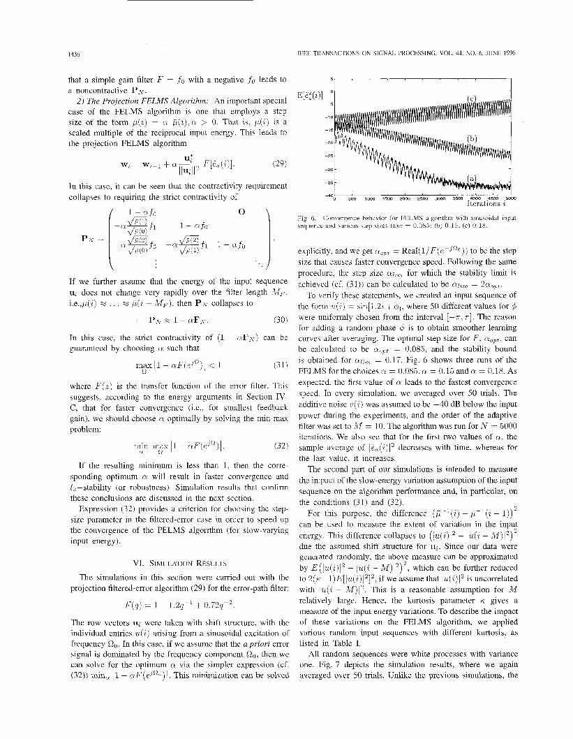
Fig. 6. sequence and various step-sizes (a)o = 0.085; (b) 0.15; (c) 0.18.

Convergence behavior for E L M S algorithm with sinusoidal input

explicitly, and we get aOpt = Real(l/F(e-j"O))) to be the step size that causes faster convergence speed. Following the same procedure, the step size allm for which the stability limit is achieved (cf. (31)) can be calculated to be cqim = 2aopt.

To verify these statements, we created an input sequence of the form n(a) = sin[1.22 + qb]? where 50 different values for 4 were uniformly chosen from the interval [-T? T ] . The reason for adding a random phase 4 is to obtain smoother learning curves after averaging. The optimal step size for F , aOpt, can be calculated to be Q,~,~ = 0.085, and the stability bound is obtained for a[irn = 0.17. Fig. 6 shows three runs of the FELMS for the choices N = 0.085, a = 0.15 and Q = 0.18. As expected, the first value of Q leads to the fastest convergence speed. In every simulation, we averaged over 50 trials. The additive noise ~ ( i ) was assumed to be -40 dB below the input power during the experiments, and the order of the adaptive filter was set to M = 10. The algorithm was run for N = 5000 iterations. We also see that for the first two values of a, the sample average of I E, ( 2 ) 1 decreases with time, whereas for the last value, it increases.

The second part of our simulations is intended to measure the impact of the slow-energy variation assumption of the input sequence on the algorithm performance and, in particular, on the conditions (31) and (32).

For this purpose, the difference ( p - ' ( i ) - p-'(2 - 1)) can be used to measure the extent of variation in the input energy. This difference collapses to (iu(i)i2 - lu(i - M)I2) due the assumed shift structure for ui. Since our data were generated randomly, the above measure can be approximated by E(lu(i)12 - lu(i - LW)12)2, which can be further reduced to 2 ( ~ - 1 ) E [ I ~ ( i ) i ~ ] ~ , if we assume that Iu(i)I2 is uncorrelated with lu(i - M ) / ' . This is a reasonable assumption for M relatively large. Hence, the kurtosis parameter K. gives a measure of the input energy variations. To describe the impact of these variations on the FELMS algorithm, we applied various random input sequences with different kurtosis, as listed in Table I.

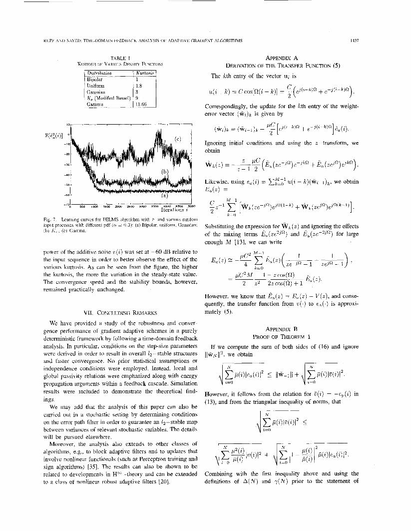
All random sequences were white processes with variance one. Fig. 7 depicts the simulation results, where we again averaged over 50 trials. Unlike the previous simulations, the

2

2

RUPP AND SAYED TIME-DOMAIN FEEDBACK ANALYSIS OF ADAPTIVE GRADIENT ALGORITHMS

I N

1437

N

TABLE I KURTOSIS OF VARIOUS DENSITY FUNCTIONS

Distribution I Kurtosis Bipolar 11 Uniform Gaussian KO (Modified Bessel) 9

11.66

i o I

I 0 500 iW0 1500 2000 25W 3ooo 3500 4000 4500 5000

-70

Iterations i

Fig. 7. Lcarning curves for FELMS algorithm with F and various random input proccsses with different pdf ((I = 0.3): (a) Bipolar, uniform, Gaussian; (b) I<(,; (c) Gamma.

power of the additive noise ~ ( i ) was set at -60 dB relative to the input sequence in order to better observe the effect of the various kurtosis. As can be seen from the figure, the higher the kurtosis, the more the variation in the steady-state value. The convergence speed and the stability bounds, however, remained practically unchanged.

VII. CONCLUDING REMARKS

We have provided a study of the robustness and convergence performance of gradient adaptive schemes in a purely deterministic framework by following a time-domain feedback analysis. In particular, conditions on the step-size parameters were derived in order to result in overall 12-stable structures and Pdster convergence. No prior statistical assumptions or independence conditions were employed. Instead, local and global passivity relations were emphasized along with energy propagation arguments within a feedback cascade. Simulation results were included to demonstrate the theoretical findings.

We may add that the analysis of this paper can also be carried out in a stochastic setting by determining conditions on the error path filter in order to guarantee an 12-stable map between variances of relevant stochastic variables. The details will be pursued elsewhere.

Moreover, the analysis also extends to other classes of algorithms, e.g., to block adaptive filters and to updates that involve nonlinear functionals (such as Perceptron training and sign algorithms) [35]. The results can also be shown to be related to developments in H"-theory and can be extended to a class of nonlinear robust adaptive filters [20].

APPENDIX A

The kth entry of the vector ui is

DERIVATION OF THE TRANSFER FUNCTION ( 5 )

Correspondingly, the update for the kth entry of the weight- error vector ( w i ) k is given by

Ignoring initial conditions and using the z - transform, we obtain

Likewise, using e,(i) = CEi' u(i - k)(wi-~)~, we obtain E,(z) =

Substituting the expression for W, (2) and ignoring the effects of the mixing terms &(ze2jn) and ~!?,(ze-~j") for large enough M [13], we can write

pC2M 1 - zcos(R) E, ( z ) . - -

2 2 2 - 2xcos(R) + 1

However, we know that f i a ( x ) = E,(x) + V ( z ) , and consequently, the transfer function from v(.) to e,(.) is approximately (5).

APPENDIX B PROOF OF THEOREM 1

If we compute the sum of both sides of (16) and ignore llwN112, we obtain

\1 C f i ( i ) l e a ( i ) I 2 5 11~-111 + CC1(i)IN2. i = O 4 i=o

However, it follows from the relation for V ( i ) = -.e,(i) in (13), and from the triangular inequality of norms, that

I N

Combining with the first inequality above and using the definitions of A(N) and y(N) prior to the statement of

1438 IEEE TRANSACTIONS ON SIGNAL PROCESSING, VOL. 44, NO. 6, JUNE 1996

Theorem 1, we conclude that

lN

M F

\ a=O \ 2=0

When (1 - A ( N ) ) > 0, we conclude that (17) holds As for the second bound, we note that

z = o i =O

and use similar arguments to the above to conclude that (18) holds.

APPENDIX C DERIVATION OF THE BOUND IN LEMMA 2

Define, for notational convenience, a( i ) = p(i)/,G(i). If we substitute .(i) = a ( i )u ( i ) - (1 - a(i))ecL(i) into (15), we get the following equality:

(2 - 4 2 ) ) [IIW + P(L)lea(i!12] = 1

d e n ( i ) where the expression for the denominator is

(1 - a ( i ) ) [ p ( i ) ( u ( i ) e z ( i ) + u * ( i ) e a ( i ) ) ] -

(1 - .(‘i)) [ l lWiIl2 + llwi-lIl*] ’

We now verify that for 1 5 a( i ) < 2

- { p ( i ) [ u ( i ) e z ( i ) + v * ( i ) e , ( i ) ] - llwii12 ~ ~lwi-~l12} 2 0.

Indeed, if we substitute for wz, as given by (3), and use & ( i ) = e,( i ) + v ( i ) = u,w,-~ + u ( i ) , we obtain that the above inequality is equivalent to verifying the nonnegativity of the following expression:

where the central matrix is

1 21 + p( i ) (a ( i ) - 2)ufu; p(i)(a(i) - 2)uf i)(C?(i) - 2)u; Ai) .(a)

We now verify that the central matrix is positive semidefinite. Its top left-comer block is positive semidefinite, and its Schur complement S can be seen to be

2p( i )a!( i ) (a!( i ) - 1) 2 + .(i)(a(i) - 2)

S =

REFERENCES

[ l ] P. P. Khargonekar and K. M. Nagpal, “Filtering and smoothing in an H=- setting,” IEEE Trans. Autoinat. Contr., vol. 36, pp. 151-166, 1991.

[2] M. Green and D. J. N. Limebeer, Lineur Robust Control. Englewood Cliffs. NJ: Prentice-Hall, 1995.

[3] K. Zhou. J. C. Doyle, and K. Glover, Robust and Optimal Control. Englewood Cliffs, NJ: Prentice-Hall, 1996.

[4] I. Yaesh and U. Shaked, “H”-optimal estimation: The discrete time case.” in Proc. Inter. Symp. Mathematical Theory Networks Syst., Kobe, Japan. June 1991, pp. 261-267.

[SI B. Hassibi. A. H. Sayed, and T. Kailath, “Linear estimation in Krein spaces-Part 11: Applications,” IEEE Trans. Automat. Contr., vol. 41, pp. 3 4 4 9 , Jan. 1996.

[6] M. Rupp. “Bursting in the LMS algorithm,” IEEE Trans. Signal Pro- cessing, vol. 43, pp. 2414-2417, Oct. 1995.

171 B. Widrow, “Adaptive sampled-data systems,” in Proc. Is/ IFAC Conn., ~~

Moscow, U.S.S.R., 1960. 181 I. D. Landau, Aduptive Control-The Model Reference ADproach. New .. ~~

York: Dekker, 1979. 191 L. Ljung and T. Soderstrom, Theory and Practice of’Recursive Identif-

cation. [ 101 I. D. Landau. “A feedback system approach to adaptive filtering,” IEEE

Trans. Zrzform. Theory, vol. IT-30, Mar. 1984. [ 111 H. K. Khalil, Nonlinear Systems. [ 121 M Vidyasagar. Nonlinear Systems Analysis. Englewood Cliffs, NJ:

Prentice-Hall, 1993, 2nd ed. [I31 J. R. Glover, Jr.. “Adaptive noise canceling applied to sinusoidal

interferences.” IEEE Trans. Acoust., Speech, Signal Processing, vol. ASSP-25. pp. 484491, Dec. 1977.

[14] P. M. Clarkson and P. R. White, “Simplified analysis of the LMS adaptive filter using a transfer function approximation,” ZEEE Trans. Acoust., Speech, Signal Processing, vol. ASSP-35, pp. 987-993, July 1987.

[I51 E. Widrow and S. D. Stearns, Aduplive Signal Processing. Englewood Cliffs. NJ: Prentice-Hall, Signal Processing Series, 1985.

[I61 A. H. Sayed and M. Rupp, “On the robustness, convergence, and minimax performance of instantaneous-gradient adaptive filters,” in Proc. A.\ilomur CO$ Signals, Syst. Comput., Oct. 1994, pp. 592-596.

1171 ~. ”A time-domain feedback analysis of adaptive gradient algorithms via the small gain theorem,” in Proc. SPIE Con$ Advanced Signal Processing: Algorithms, Architectures, Implementations, vol. 2563, July 1995. San Diego. pp. 458-469.

[18] B. Hassibi. A. H. Sayed, and T. Kailath, “LMS is Ha optimal,” in Proc. Con5 Decision Contr., vol. 1, San Antonio, Dec. 1993, pp. 74-79; also, ZEEE Truizs. Signal Processing, vol. 44, pp. 267-280, Feb. 1996.

[I91 A. H. Sayed and T. Kailath, “A state-space approach to adaptive RLS filtering,” IEEE Signal Processing Mug., vol. 11, no. 3, pp. 18-60, July 1994.

[20] A. H. Sayed and M. Rupp, “A class of nonlinear adaptive Ha-filters with guaranteed /%-stability,” Proc. IFAC Symp. Nonlinear Conlr. Sys/. Der., vol. 1. Tahoe City, CA, June 1995, pp. 455460; also, Automutica, to be published.

[21] V. Solo and X. Kong. Adaptive Signal Processing Algorithms: Stability uiid Performance.

I221 N. J. Bershad. “Analysis of the normalized LMS algorithm with Gauss- ian inputs,” IEEE Trans. Acoust., Speech, Sifnul Processinf, vol. ASSP-

Cambridge, MA: MIT Press, 1983.

New York: MacMillan, 1992.

Englewood Cliffs, NJ: Prentice-Hall, 1995.

34. no. 4, pp. 793-806, Aug. 1986. [23] M. Rupp. “The behavior of LMS and NLMS algorithms in the presence ..

of spherically invariant processes,” IEEE Trans. Signal Processing, vol. 41, pp. 1149-1160, Mar. 1993.

[24] D. R. Morgan, “An analysis of multiple correlation cancellation loops with a filter in the auxiliary path,” IEEE Trans. Acoust., Speech, Signal Processing, vol. ASSP-28, pp. 454467, Aug. 1980.

[25] L. J. Eriksson, “Development of the filtered-U algorithm for active noise control,” J. Acoust. Soc. Amer., vol. 89, no. 1, pp. 257-265, Apr. 1991.

[26] S. Laugesen and S. Elliott, “Multichannel active control of random noise in a small reverberant room,” ZEEE Trans. Speech, Audio Processing, vol. 1, pp. 241-249, Apr. 1993.

[27] M. Rupp-and A. H. Saykd, “Modified FxLMS algorithms with improved convergence performance,” in P roc. 29th Asilomar Conf Si,qnals, Syst. which is larger than or equal to zero for a( i ) between one and

“ I

two. It then follows that we can write Compu;., Pacific Grove, CA, Oct. 1995. [28] -, “On the stability and convergence of Feintuch’s algorithm for

adaptive IIR filtering,” in Proc. ZCASSP, vol. 2, Detroit, MI, May 1995, pp. 1388-1391.

[29] E. Bjarnason, “Noise cancellation using a modified form of the filtered-XLMS algorithm,” in Proc. Eusipco Signal Processing V , Briissel, Belgium, 1992.

( 2 - 4 2 ) ) [IIW + P(i)lea(i)12] 4 1

a( 2 ) I IWi- 1 I I * + p ( i ) a( 1:) l?I (i) l 2 which establishes the result of Lemma 2.

KUPP AND SAYED: TIME-DOMAIN FEEDBACK ANALYSIS OF ADAPTIVE GRADIENT ALGORITHMS 1439

1301 I. Kim, H. Na, K. Kim, and Y. Park, “Constraint filtered-x and filtered- U algorithms for the active control of noise in a duct,” J . ACOUS~. Soc. Amer., vol. 95, no. 6, pp. 3397-3389, June 1994.

1311 S. Dasgupta, J. S. Garnett, and C. R. Johnson, Jr., “Convergence of an adaptive filter with signed filtered error,” IEEE Truns. Signul Processing, vol. 42, pp. 946-950, Apr. 1994.

[32] P. L. Feintuch, “An adaptive recursive LMS filter,” Proc.. I E E , vol. 64, pp. 1622-1624, Nov. 1976.

[33] M. G. Larimore, J. R. Treichler, and C. R. Johnson, “SHARF: An algorithm for adapting IIR digital filters,” IEEE Trans. Acoust., Speech, Signal Processing, vol. ASSP-28, pp. 428-440, Aug. 1980.

[34] S. J. Elliot, I. M. Stothers, and P. A. Nelson, “A multiple error LMS algorithm and its application to the active control of sound and vibration,” IEEE Truns. Acoustics, Speech, Signal Processing vol. ASSP-35, pp. 1423-1434, Oct. 1987.

1351 A. H. Sayed and M. Rupp, “A feedback analysis of Perceptron learning for neural networks, to appear in Proc. 29th Asilomur Conf Signuls, Syst. Comput., Pacific Grove, CA, Oct. 1995.

Markus Rupp received the Diploma in electrical engineering from FHS, Saarbruecken, Germany, and Universitaet of Saarbruecken in 1984 and 1988, reqpectively During this time, he was a150 a lecturer in digital signal processing and high frequency tech- niques at the FHS. He received the Doctoral degree in 1993 summa cum laude at the TH Darmstadt in the field of dcou5tical echo cancellation

He received the DAAD Post-Doctoral fellowship and .,pent November 1993 until September 1995 with the Department of Electrical and Computer

Engineering of the University of California, Santa Barbdra. Since October 1995, he has been with the AT&T Wireleqs Technology Research Group, Holmdel, NJ, where he ic currently working on new adaptive equdhzation schemes His interem involve algorithm., for speech applications, speech enhancement and recognition, echo compensation, ddaptive filter theory, H, -filtering, neural nets, classification algorithms, and signal detection

Ali H. Sayed (M’92) was born in SZo Paulo, Brazil In 1981, he graduated in first place in the National Lebanese Baccalaureat, with the highest Score in the history of the examination In 1987, he received the degree of engineer in electrical engineenng from the University of Silo Paulo, Brazil, and was the first place graduate of the School of Engineering. In 1989, he received, with distinction, the M.S. degree in electrical engineering from the University of Silo Paulo, Brazil, and was awarded a FAPESP fellowship for overseas studies. In 1992, he received

the Ph D degree in electrical engineering from Stanford University, Stanford, CA.

From September 1992 to August 1993, he was a Research Associate with the Information Systems Laboratory at Stanford University, after which he joined, as an Assistant Profewor, the Department of Electrical and Computer Engineering at the University of California, Santa Barbara His research interests are in the areas of adaptive and statistical signal processing, linear and nonlinear filtering and ectimation, interplays between signal processing and control methodologies, interpolation theory, and structured computations in systems and mathematics.

Dr Sayed is a member of SIAM and ILAS. He was awarded the Inmute of Engineering Prize and the Conde Armando Alvares Penteado Prize, both in 1987 in Brazil. He is a recipient of a 1994 NSF Research Initiation Award and of the 1996 IEEE Donald G Fink Prize

A time-domain feedback analysis of filtered-error adaptive gradient algorithms

Documents

Transcript of A time-domain feedback analysis of filtered-error adaptive gradient algorithms